Embed Size (px)
Citation preview
Systematic Mortality Risk: An Analysis ofGuaranteed Lifetime Withdrawal Benefits in
Variable Annuities
This version: 20 May 2013
Man Chung Fung a, Katja Ignatieva b 1 , Michael Sherris c
aSchool of Risk and Actuarial Studies, University of New South Wales, Sydney,Australia ([email protected])
bSchool of Risk and Actuarial Studies, University of New South Wales, Sydney,Australia ([email protected])
cCEPAR, School of Risk and Actuarial Studies, University of New South Wales,Sydney, Australia ([email protected])
JEL Classification: G22, G23, G13
Abstract
Guaranteed lifetime withdrawal benefits (GLWB) embedded in variable annuitieshave become an increasingly popular type of life annuity designed to cover sys-tematic mortality risk while providing protection to policyholders from downsideinvestment risk. This paper provides an extensive study of how different sets offinancial and demographic parameters affect the fair guaranteed fee charged fora GLWB as well as the profit and loss distribution, using tractable equity andstochastic mortality models in a continuous time framework. We demonstrate thesignificance of parameter risk, model risk, as well as the systematic mortality riskcomponent underlying the guarantee. We quantify how different levels of equity ex-posure chosen by the policyholder affect the exposure of the guarantee providers tosystematic mortality risk. Finally, the effectiveness of a static hedge of systematicmortality risk is examined allowing for different levels of equity exposure.
Key words: variable annuity, guaranteed lifetime withdrawal benefits (GLWB),systematic mortality risk, parameter risk, model risk, static hedging
1 Corresponding author: School of Risk and Actuarial Studies, Australian Schoolof Business, University of New South Wales, Sydney, NSW-2052, Australia. Email:[email protected]; Tel: +61 2 9385 6810.
1
1 Introduction
Variable annuities (VA), introduced in the 1970s in the US, have proven to be pop-ular among investors and retirees especially in North America and Japan. VA areinsurance contracts which allow policyholders to invest their retirement savings inmutual funds. They are attractive because policyholders gain exposure to the equitymarkets with benefits based on the performance of the underlying funds, along withreturn guarantees as well as tax advantages. In addition to the VA, policyholderscan elect guarantees to provide minimum benefits with the payment of guaranteefees. Since the 1990s, two kinds of embedded guarantees have been offered in thesepolicies. These include the Guaranteed Minimum Death Benefits (GMDB) and theGuaranteed Minimum Living Benefits (GMLB), see Hardy (2003) and Ledlie et al.(2008). There are four types of guarantee that fall into the category of GMLB:
• Guaranteed Minimum Accumulation Benefits (GMAB)• Guaranteed Minimum Income Benefits (GMIB)• Guaranteed Minimum Withdrawal Benefits (GMWB)• Guaranteed Lifetime Withdrawal Benefits (GLWB)
According to LIMRA 2 , the election rates of GLWB, GMIB, GMAB and GMWB inthe fourth quarter of 2011 in the US were 59%, 26%, 3% and 2%, respectively. Thepopularity of the GLWB can be attributed to its flexibility in that the policyholdercan specify how much he/she wants to withdraw every year for the lifetime of theinsured regardless of the performance of the investment, subject to a limited nominalyearly amount. After the death of the insured, any savings remaining in the accountare returned to the insured’s beneficiary. GLWB provide a life annuity with flexiblefeatures compared to traditional life annuity contracts.
As a type of a life annuity with benefits linked to the equity market, insurers whooffer a GLWB embedded in variable annuities are subject to equity risk, interest raterisk, withdrawal risk and, in particular, systematic mortality risk. Non-systematic,or idiosyncratic mortality risk, is diversifiable, whereas systematic mortality risk, orlongevity risk, cannot be eliminated through diversification. Systematic mortalityrisk arises due to the stochastic, or unpredictable, nature of survival probabilities.Insurance providers offering GLWB face systematic mortality risk since the guaranteepromises to the insured a stream of income for life, even if the investment accountis depleted. Stochastic mortality models, often implemented in an intensity-basedframework, e.g. Biffis (2005), are required to quantify this systematic mortality risk.
1.1 Motivation and Contribution
Following the global financial crisis in 2007-2008, VA providers have suffered un-expectedly large losses arising from the benefits provided by the different types ofguarantee being too generous. High volatility of equity markets during this period
2 http : //www.limra.com/default.aspx
2
resulted in unexpectedly high hedging costs and exacerbated the difficulty in man-aging the risks underlying the guarantees. 3 Guarantees were inherently difficult toprice and manage because of their long term nature. Along with the equity risk,guarantees offering lifetime income were exposed to systematic mortality risk fromhigher than expected mortality improvements. An important example of a guaranteeproduct where the risks are not well understood is the GLWB.
Bacinello et al. (2011) set out the three steps required for a reliable risk managementprocess. First is risk identification. For the benefit and the premium component of aguarantee, different sources of risk, whether hedgeable or not, need to be determined. 4
The second step involves risk assessment. The long term nature and complex payoutstructure of these guarantees involves a range of risks. An assessment of the interac-tions between these risks is essential when considering an adequate risk managementprogram. Risk assessment is also used to determine which sources of risk have thelargest impact on the pricing and risk management of the guarantee. The final step isthe risk management action. Risk management for these guarantees involves capitalreserving and hedging (Hardy (2003) and Ledlie et al. (2008)). Selecting the appro-priate hedge instruments and determining hedging frequency, in particular, static ordynamic hedging, need to be considered, along with constraints such as transactioncosts and liquidity of the hedge instruments. A reliable risk management process isparticularly important for GLWB since it is a long term contract, lasting on averagefor several decades, and involves many different risks. Due to its recent popularity,VA providers have large exposures that have grown with the GLWB as an underlyingguarantee.
The significance of GLWB products in providing longevity insurance for individualsdesiring a guaranteed income in retirement with equity exposure has been recognized.Despite this, the analysis of systematic mortality risk in GLWB, along with its inter-action with other risks, has not been studied in detail. Studies have focussed on only aparticular aspect of this risk. One of the earliest modeling frameworks that focuses onGLWB is discussed in Holz et al. (2007), who take into account policyholder’s behav-ior and different product features. Kling et al. (2011) focus on volatility risk. Piscopoand Haberman (2011) assess mortality risk in GLWB but not the other risks andtheir interactions. Bacinello et al. (2011) and Ngai and Sherris (2011) include GLWBbut only as part of a specific study of pricing or hedging guarantees/annuities.
Papers that investigate the impact of systematic mortality risk on guarantees otherthan GLWB include Ballotta and Haberman (2006) who value guaranteed annuityoptions (GAOs) and provide sensitivity analysis taking into account the interest raterisk and the systematic mortality risk. Kling et al. (2012) offer an analysis similar toBallotta and Haberman (2006), but considering both, GAOs and guaranteed minimalincome benefits (GMIB), and taking into account different hedging strategies. Ziveyiet al. (2013) price European options on deferred insurance contracts including pureendowment and deferred life annuity (i.e. GAO) by solving analytically the pricingpartial differential equation in a presence of systematic mortality risk.
3 See for instance “A challenging environment”, June 2008 and “A balanced structure?”,February 2011 in the Risk Magazine.4 For instance, uncertainty stemming from the behavior of policyholders is an unhedgeablerisk, which requires insurance companies to assess policyholders general past behavior.
3
A detailed analysis of the impact of systematic mortality risk on valuation and hedg-ing, as well as its interaction with other risks underlying the GLWB is required. Theseissues are the focus of the present paper. We apply the risk management process de-scribed above to analyze equity and systematic mortality risks underlying the GLWB,as well as their interactions. We use risk measures and the profit and loss (P&L) dis-tribution in order to identify, assess and partially mitigate financial and demographicrisks, for the GLWB guarantee. P&L analysis has proven to be useful in assessing sys-tematic mortality risk in pension annuities, see Hari et al. (2008). We use the affinemortality model approach. Dahl and Moller (2006) considers a time inhomogeneoussquare root process, Schrager (2006) and Biffis (2005) propose multi-factor affine pro-cesses which capture the evolution of mortality intensity for all ages simultaneously.A concise survey of mortality modeling and the development of longevity market canbe found in Cairns et al. (2008). Our aim is to adopt a tractable model given thecomplex nature of the product.
We quantify how different sets of financial and demographic parameters affect theguarantee fees. We assess their effects on the P&L distributions, if the parametersare different from the “true” parameters of the underlying dynamics. Parameter riskis shown to be a significant risk reflecting the long term nature of the GLWB, giventhe exposure for the lifetime of the insured in a portfolio. We consider model risk byconsidering the case where guarantee providers assume mortality to be deterministicwhen the mortality is stochastic in its nature.
The paper also considers the capital reserve required due to the lack of hedging in-struments to hedge the longevity risk. The paper uses P&L analysis to show thatdifferent levels of equity exposure chosen by the insured have, in the presence ofsystematic mortality risk, a significant impact on the risk of the GLWB from theguarantee providers’ perspective. Finally, the effectiveness of a static hedge of sys-tematic mortality risk is also assessed allowing for different levels of equity exposure.
The remainder of the paper is organized as follows. Section 2 outlines the generalfeatures of GLWB including identification of risks and additional product features,along with the benefit and the premium components of the guarantee. Section 3specifies the continuous time models used for the underlying equity and systematicmortality risk. Section 4 evaluates the GLWB using two approaches, which are shownto be equivalent. It generalizes the pricing result of the GMWB in Kolkiewicz andLiu (2012) to the case of the GLWB. Sensitivity analysis is conducted in Section5, which quantifies the sources of risk with the larger impact on pricing of GLWB.Section 6 analyzes the impact of different types of risk on the P&L distributionsof the guarantee, without incorporating any hedging strategies. Different levels ofequity exposure, parameter risk and model risk are considered. Section 7 studies theeffectiveness of a static hedge of systematic mortality risk using S-forward’s takinginto account different levels of equity exposure. Section 8 summarizes the results andprovides further concluding remarks.
4
2 Features of GLWB
A variable annuity (VA) is an insurance product where a policyholder invests his orher retirement savings in a mutual fund in the form of an investment account managedby an insurance company. VAs are attractive because the investment enjoys certaintax benefits along with investment in the equity market. A VA with a GLWB riderguarantees payment of a capped amount of income that can be withdrawn from theaccount every year for the lifetime of the policyholder, even if the investment accountis depleted before the policyholder dies. Any remaining value in the account will bereturned to the policyholder’s beneficiary. In return, the policyholder is required topay a guarantee fee every year, which is proportional to the investment account value.
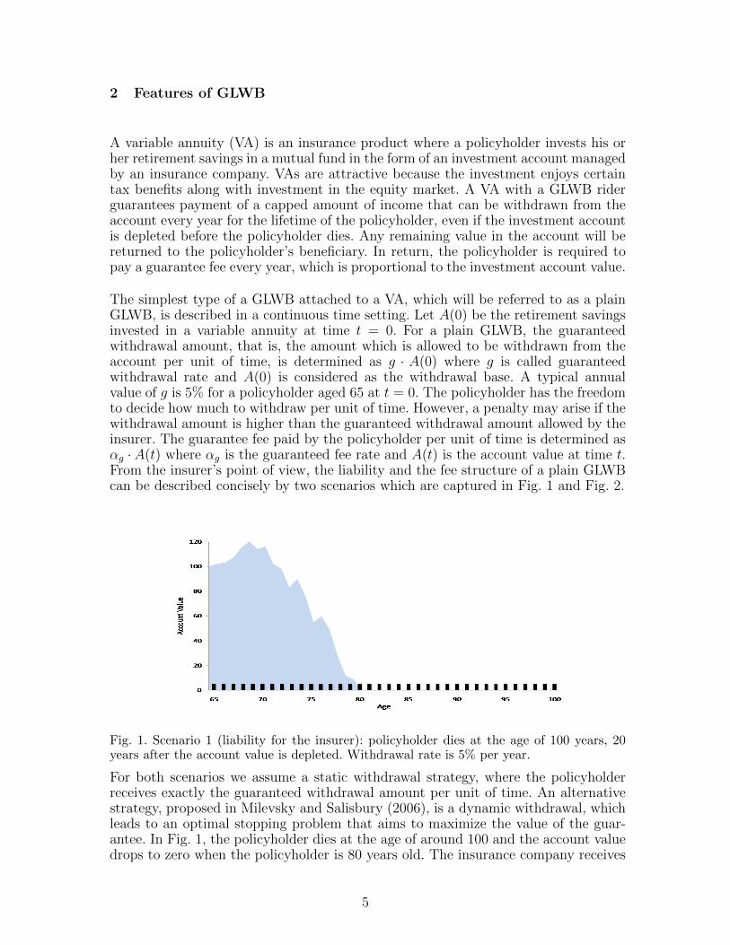
The simplest type of a GLWB attached to a VA, which will be referred to as a plainGLWB, is described in a continuous time setting. Let A(0) be the retirement savingsinvested in a variable annuity at time t = 0. For a plain GLWB, the guaranteedwithdrawal amount, that is, the amount which is allowed to be withdrawn from theaccount per unit of time, is determined as g · A(0) where g is called guaranteedwithdrawal rate and A(0) is considered as the withdrawal base. A typical annualvalue of g is 5% for a policyholder aged 65 at t = 0. The policyholder has the freedomto decide how much to withdraw per unit of time. However, a penalty may arise if thewithdrawal amount is higher than the guaranteed withdrawal amount allowed by theinsurer. The guarantee fee paid by the policyholder per unit of time is determined asαg ·A(t) where αg is the guaranteed fee rate and A(t) is the account value at time t.From the insurer’s point of view, the liability and the fee structure of a plain GLWBcan be described concisely by two scenarios which are captured in Fig. 1 and Fig. 2.
Fig. 1. Scenario 1 (liability for the insurer): policyholder dies at the age of 100 years, 20years after the account value is depleted. Withdrawal rate is 5% per year.
For both scenarios we assume a static withdrawal strategy, where the policyholderreceives exactly the guaranteed withdrawal amount per unit of time. An alternativestrategy, proposed in Milevsky and Salisbury (2006), is a dynamic withdrawal, whichleads to an optimal stopping problem that aims to maximize the value of the guar-antee. In Fig. 1, the policyholder dies at the age of around 100 and the account valuedrops to zero when the policyholder is 80 years old. The insurance company receives
5
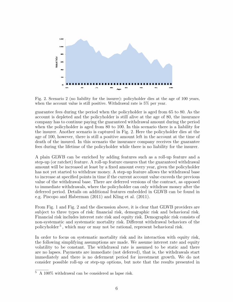
Fig. 2. Scenario 2 (no liability for the insurer): policyholder dies at the age of 100 years,when the account value is still positive. Withdrawal rate is 5% per year.
guarantee fees during the period when the policyholder is aged from 65 to 80. As theaccount is depleted and the policyholder is still alive at the age of 80, the insurancecompany has to continue paying the guaranteed withdrawal amount during the periodwhen the policyholder is aged from 80 to 100. In this scenario there is a liability forthe insurer. Another scenario is captured in Fig. 2. Here the policyholder dies at theage of 100, however, there is still a positive amount left in the account at the time ofdeath of the insured. In this scenario the insurance company receives the guaranteefees during the lifetime of the policyholder while there is no liability for the insurer.
A plain GLWB can be enriched by adding features such as a roll-up feature and astep-up (or ratchet) feature. A roll-up feature ensures that the guaranteed withdrawalamount will be increased at least by a fixed amount every year, given the policyholderhas not yet started to withdraw money. A step-up feature allows the withdrawal baseto increase at specified points in time if the current account value exceeds the previousvalue of the withdrawal base. There are deferred versions of the contract, as opposedto immediate withdrawals, where the policyholder can only withdraw money after thedeferred period. Details on additional features embedded in GLWB can be found ine.g. Piscopo and Haberman (2011) and Kling et al. (2011).
From Fig. 1 and Fig. 2 and the discussion above, it is clear that GLWB providers aresubject to three types of risk: financial risk, demographic risk and behavioral risk.Financial risk includes interest rate risk and equity risk. Demographic risk consists ofnon-systematic and systematic mortality risk. Different withdrawal behaviors of thepolicyholder 5 , which may or may not be rational, represent behavioral risk.
In order to focus on systematic mortality risk and its interaction with equity risk,the following simplifying assumptions are made. We assume interest rate and equityvolatility to be constant. The withdrawal rate is assumed to be static and thereare no lapses. Payments are immediate (not deferred), that is, the withdrawals startimmediately and there is no deferment period for investment growth. We do notconsider possible roll-up or step-up options, but note that the results presented in
5 A 100% withdrawal can be considered as lapse risk.
6
the following sections can be generalized when additional features are incorporatedin the contract.
3 Model Specification
We base our analysis on tractable continuous-time models to capture equity andsystematic mortality risk underling GLWB in variable annuities. Let (Ω,F ,P) be afiltered probability space where P is the real world probability measure. The filtrationFt is constructed as
Gt = σ(W1(s),W2(s)) : 0 ≤ s ≤ tHt = σ1τ≤s : 0 ≤ s ≤ tFt = Gt ∨Ht
where Gt is generated by two independent standard Brownian motions, W1 and W2,which are associated with the uncertainties related to equity and mortality inten-sity, respectively. The subfiltration Ht represents information set that would indicatewhether the death of a policyholder has occurred before time t. The stopping timeτ is interpreted as the remaining lifetime of an insured. For a detailed exposition ofmodeling mortality under the intensity-based framework refer to Biffis (2005).
3.1 Investment Account Dynamics
The policyholder can invest his or her retirement savings in an investment fund thathas both, equity and fixed income exposure. Under the real world probability measureP, we assume that the equity component follows the geometric Brownian motion
dS(t) = µS(t)dt+ σS(t)dW1(t), (3.1)
and the fixed income investment is represented by the money market account B(t)with dynamics dB(t) = r B(t)dt where the interest rate r is constant. Let δ1(t) andδ2(t) denote the number of units invested in S(·) and B(·), respectively. The self-financing investment fund V (·) has the following dynamics
dV (t) = δ1(t)dS(t) + δ2(t)dB(t)
= (µδ1(t)S(t) + rδ2(t)B(t))dt+ σδ1(t)S(t)dW1(t)
= (µπ(t) + r(1− π(t)))V (t)dt+ σπ(t)V (t)dW1(t) (3.2)
where the fraction π(·) is defined as π(t) = δ1(t)S(t)V (t)
, and is interpreted as the propor-
tion of the retirement savings being invested in the equity component. Since short-selling is not allowed, we set 0 ≤ π(·) ≤ 1.
Because of the election of GLWB, the investment account A(·) held by the policy-holder is being charged continuously with guarantee fees, denoted by fee rate αg, by
7
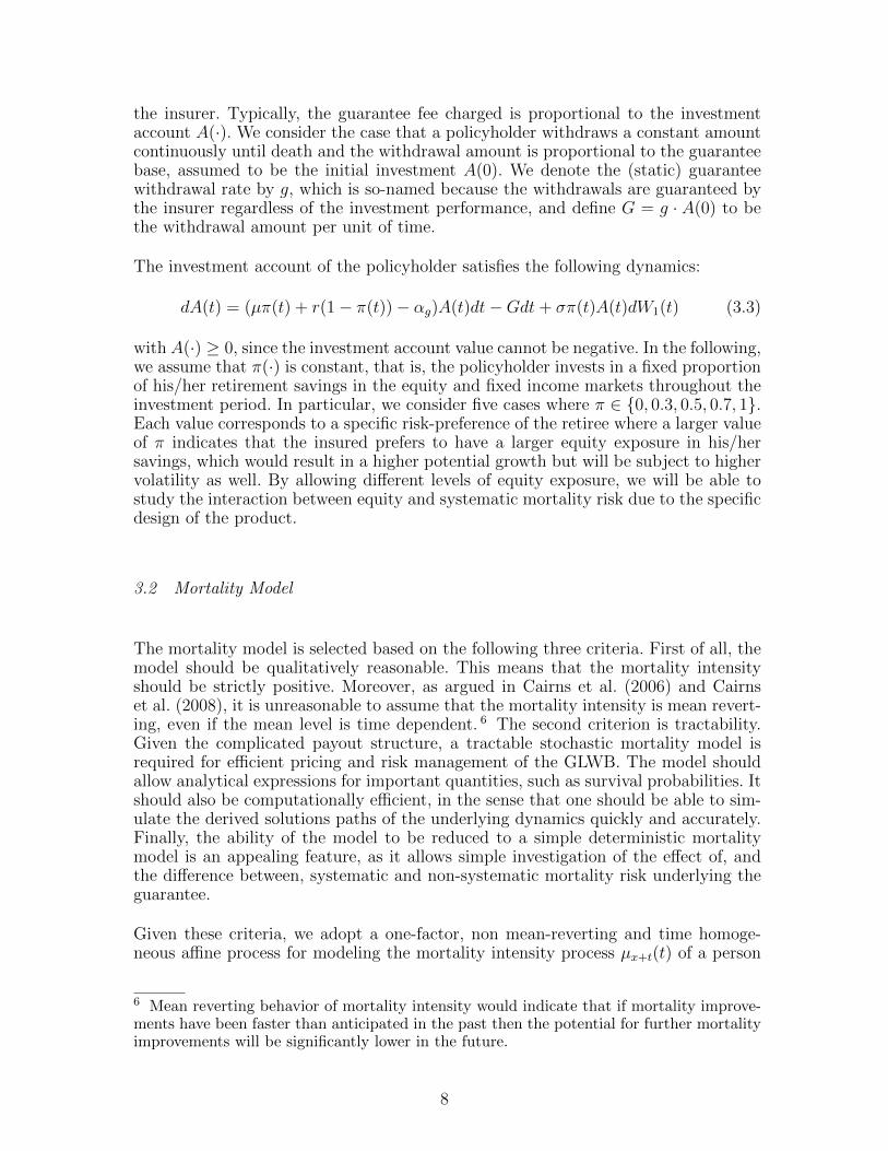
the insurer. Typically, the guarantee fee charged is proportional to the investmentaccount A(·). We consider the case that a policyholder withdraws a constant amountcontinuously until death and the withdrawal amount is proportional to the guaranteebase, assumed to be the initial investment A(0). We denote the (static) guaranteewithdrawal rate by g, which is so-named because the withdrawals are guaranteed bythe insurer regardless of the investment performance, and define G = g · A(0) to bethe withdrawal amount per unit of time.
The investment account of the policyholder satisfies the following dynamics:
dA(t) = (µπ(t) + r(1− π(t))− αg)A(t)dt−Gdt+ σπ(t)A(t)dW1(t) (3.3)
with A(·) ≥ 0, since the investment account value cannot be negative. In the following,we assume that π(·) is constant, that is, the policyholder invests in a fixed proportionof his/her retirement savings in the equity and fixed income markets throughout theinvestment period. In particular, we consider five cases where π ∈ 0, 0.3, 0.5, 0.7, 1.Each value corresponds to a specific risk-preference of the retiree where a larger valueof π indicates that the insured prefers to have a larger equity exposure in his/hersavings, which would result in a higher potential growth but will be subject to highervolatility as well. By allowing different levels of equity exposure, we will be able tostudy the interaction between equity and systematic mortality risk due to the specificdesign of the product.
3.2 Mortality Model
The mortality model is selected based on the following three criteria. First of all, themodel should be qualitatively reasonable. This means that the mortality intensityshould be strictly positive. Moreover, as argued in Cairns et al. (2006) and Cairnset al. (2008), it is unreasonable to assume that the mortality intensity is mean revert-ing, even if the mean level is time dependent. 6 The second criterion is tractability.Given the complicated payout structure, a tractable stochastic mortality model isrequired for efficient pricing and risk management of the GLWB. The model shouldallow analytical expressions for important quantities, such as survival probabilities. Itshould also be computationally efficient, in the sense that one should be able to sim-ulate the derived solutions paths of the underlying dynamics quickly and accurately.Finally, the ability of the model to be reduced to a simple deterministic mortalitymodel is an appealing feature, as it allows simple investigation of the effect of, andthe difference between, systematic and non-systematic mortality risk underlying theguarantee.
Given these criteria, we adopt a one-factor, non mean-reverting and time homoge-neous affine process for modeling the mortality intensity process µx+t(t) of a person
6 Mean reverting behavior of mortality intensity would indicate that if mortality improve-ments have been faster than anticipated in the past then the potential for further mortalityimprovements will be significantly lower in the future.
8

aged x at time t = 0, as follows:
dµx+t(t) = (a+ b µx+t(t))dt+ σµ√µx+t(t) dW2(t), µx(0) > 0. (3.4)
Here, a 6= 0, b > 0 and σµ represents the volatility of the mortality intensity.
In the special case when σµ = a = 0, the model reduces to the well-known constantGompertz specification. 7 Hence, we will be able to conveniently compare the impactof stochastic mortality with that of deterministic mortality in Sec. 6.3. The valuesof the parameters a, b and σµ are obtained by calibrating the survival curve impliedby the mortality model to the survival curve obtained from population data as doc-umented in the Australian Life Tables 2005-2007 8 , for a male aged 65. The result isreported in Table 1.
Table 1Calibrated parameters for the mortality model.
a b σµ µ65(0)0.001 0.087 0.021 0.01147
The estimated values of the parameters a and σµ indicate that the proposed mortalityintensity process in Eq.(3.4) is strictly positive 9 and is non mean-reverting. Model-ing mortality intensity using a one-factor 10 and time homogeneous affine process canreduce computational time significantly, since the model dynamics can be easily sim-ulated and used to derive analytical expressions for survival probabilities. Thus, theproposed model in Eq.(3.4) satisfies all criteria stated above.
Because of the affine and time homogeneous assumption, we have an analytical ex-pression for the survival probability sPx+t for the remaining lifetime τ of an individualaged x at time 0. Assuming that the individual is still alive at t > 0 and that σµ > 0,we obtain
sPx+t = EQt
(e−∫ t+st
µx+v(v)dv)
= C1(s)e−C2(s)µx+t(t), (3.5)
where
C1(s) =
2γe12(γ−b)s
(γ − b)(eγs − 1) + 2γ
2a
σ2µ
, C2(s) =2(eγs − 1)
(γ − b)(eγs − 1) + 2γ(3.6)
and γ =√b2 + 2σ2
µ. For details refer to Dahl and Moller (2006). The density function
7 From the Gompertz model µx(0) = yebx, we have µx+t(t) = µx(0)ebt which satisfiesEq.(3.4) with σµ = a = 0.8 http : //www.aga.gov.au/publications/#life tables9 It can be shown that if a ≥ σ2µ/2 then the mortality intensity process Eq.(3.4) is strictlypositive, see Filipovic (2009).10 Although past mortality data shows differences between the evolution of mortality ratesfor different ages, applying a multi-factor mortality model to the pricing of GLWB requiressignificant computational resources (refer to Section 4) without adding particular insightsto the main results. For this reason we restrict ourselves to a one-factor model.
9
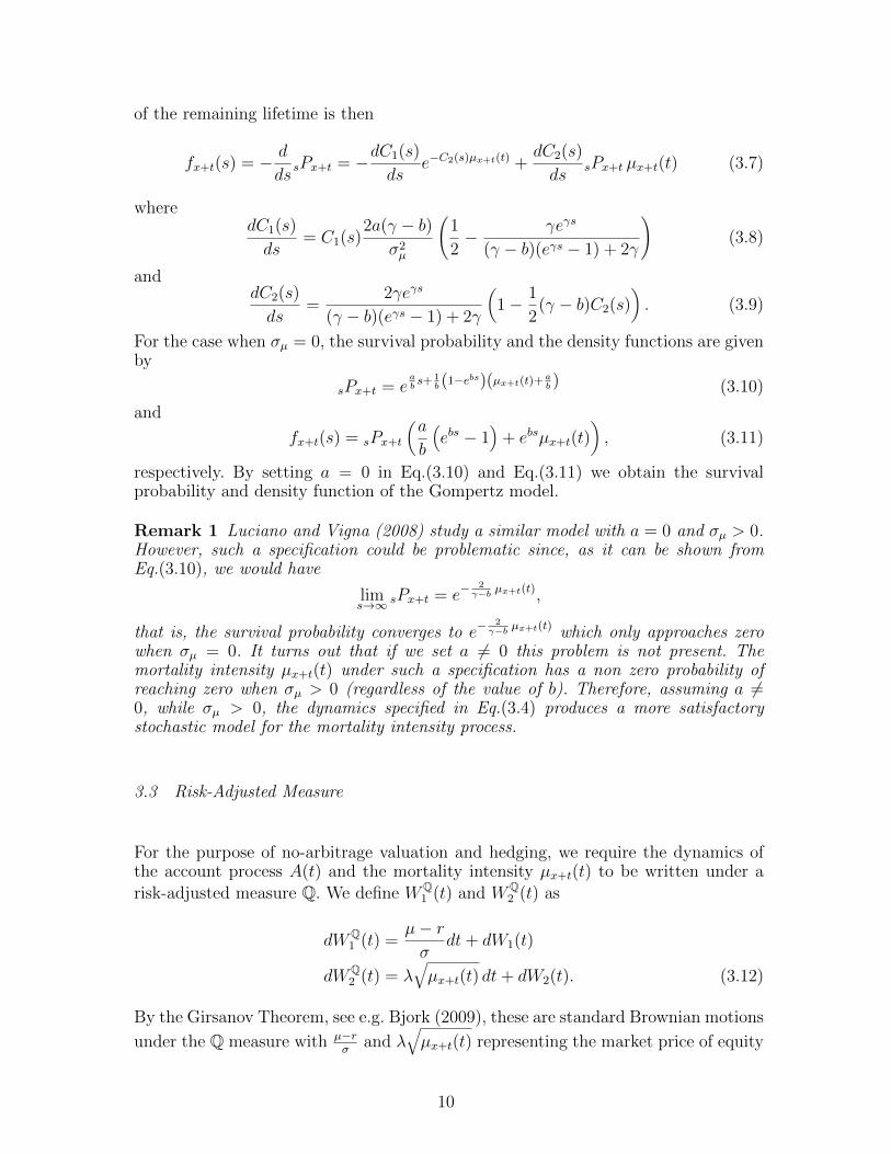
of the remaining lifetime is then
fx+t(s) = − d
dssPx+t = −dC1(s)
dse−C2(s)µx+t(t) +
dC2(s)
dssPx+t µx+t(t) (3.7)
wheredC1(s)
ds= C1(s)
2a(γ − b)σ2µ
(1
2− γeγs
(γ − b)(eγs − 1) + 2γ
)(3.8)
anddC2(s)
ds=
2γeγs
(γ − b)(eγs − 1) + 2γ
(1− 1
2(γ − b)C2(s)
). (3.9)
For the case when σµ = 0, the survival probability and the density functions are givenby
sPx+t = eabs+ 1
b (1−ebs)(µx+t(t)+ab ) (3.10)
and
fx+t(s) = sPx+t
(a
b
(ebs − 1
)+ ebsµx+t(t)
), (3.11)
respectively. By setting a = 0 in Eq.(3.10) and Eq.(3.11) we obtain the survivalprobability and density function of the Gompertz model.
Remark 1 Luciano and Vigna (2008) study a similar model with a = 0 and σµ > 0.However, such a specification could be problematic since, as it can be shown fromEq.(3.10), we would have
lims→∞ sPx+t = e−
2γ−b µx+t(t),
that is, the survival probability converges to e−2γ−b µx+t(t) which only approaches zero
when σµ = 0. It turns out that if we set a 6= 0 this problem is not present. Themortality intensity µx+t(t) under such a specification has a non zero probability ofreaching zero when σµ > 0 (regardless of the value of b). Therefore, assuming a 6=0, while σµ > 0, the dynamics specified in Eq.(3.4) produces a more satisfactorystochastic model for the mortality intensity process.
3.3 Risk-Adjusted Measure
For the purpose of no-arbitrage valuation and hedging, we require the dynamics ofthe account process A(t) and the mortality intensity µx+t(t) to be written under arisk-adjusted measure Q. We define WQ
1 (t) and WQ2 (t) as
dWQ1 (t) =
µ− rσ
dt+ dW1(t)
dWQ2 (t) = λ
õx+t(t) dt+ dW2(t). (3.12)
By the Girsanov Theorem, see e.g. Bjork (2009), these are standard Brownian motions
under the Q measure with µ−rσ
and λ√µx+t(t) representing the market price of equity
10

risk and systematic mortality risk, respectively. We can then write the investmentaccount process and the mortality intensity under Q as follows:
dA(t) = (r − αg)A(t)dt−Gdt+ π σ A(t)dWQ1 (t) (3.13)
dµx+t(t) = (a+ (b− λσµ))µx+t(t)dt+ σµ√µx+t(t)dW
Q2 (t). (3.14)
By imposing the market price of systematic mortality risk to be λ√µx+t(t), the mor-
tality intensity process is still a time homogeneous affine process under Q, as canbe seen from Eq.(3.14). 11 Thus, this specification preserves tractability of the modelwhen pricing the guarantee under Q. From Eq.(3.13) we observe that the fractionπ invested in the equity market only affects the volatility of the investment accountprocess under Q.
0 5 10 15 20 25 30 35 40 450
0.1
0.2
0.3
0.4
0.5
0.6
0.7
0.8
0.9
1
Remaining Lifetime s (year)
Su
rviv
al P
rob
ab
ility
s
P65
σµ=0.00
σµ=0.011
σµ=0.021
σµ=0.031
σµ=0.041
σµ=0.051
0 5 10 15 20 25 30 35 40 450
0.005
0.01
0.015
0.02
0.025
0.03
0.035
0.04
0.045
Remaining Lifetime s (year)
De
nsity f
65(s
)
σµ=0.00
σµ=0.011
σµ=0.021
σµ=0.031
σµ=0.041
σµ=0.051
Fig. 3. Survival probabilities and densities of the remaining lifetime of an individual aged65 with different values of σµ. Other parameters are as specified in Table 1 with λ = 0.4.
0 5 10 15 20 25 30 35 40 450
0.1
0.2
0.3
0.4
0.5
0.6
0.7
0.8
0.9
1
Remaining Lifetime s (year)
Su
rviv
al P
rob
ab
ility
s
P65
λ=−0.4
λ=0.0
λ=0.4
λ=0.8
λ=1.2
λ=1.6
0 5 10 15 20 25 30 35 40 450
0.005
0.01
0.015
0.02
0.025
0.03
0.035
0.04
0.045
Remaining Lifetime s (year)
De
nsity f
65(s
)
λ=−0.4
λ=0.0
λ=0.4
λ=0.8
λ=1.2
λ=1.6
Fig. 4. Survival probabilities and densities of the remaining lifetime of an individual aged65 with different values of λ. Other parameters are as specified in Table 1. The case λ = 0corresponds to the survival curve under P.
11 The mortality intensity process might become mean reverting, however, when b < λσµ.
11
0 0.01 0.02 0.03 0.04 0.0510
15
20
25
30
35
40
σµ
Exp
ecte
d R
em
ain
ing
Life
tim
e
0 0.5 1 1.510
15
20
25
30
35
40
λ
Exp
ecte
d R
em
ain
ing
Life
tim
e
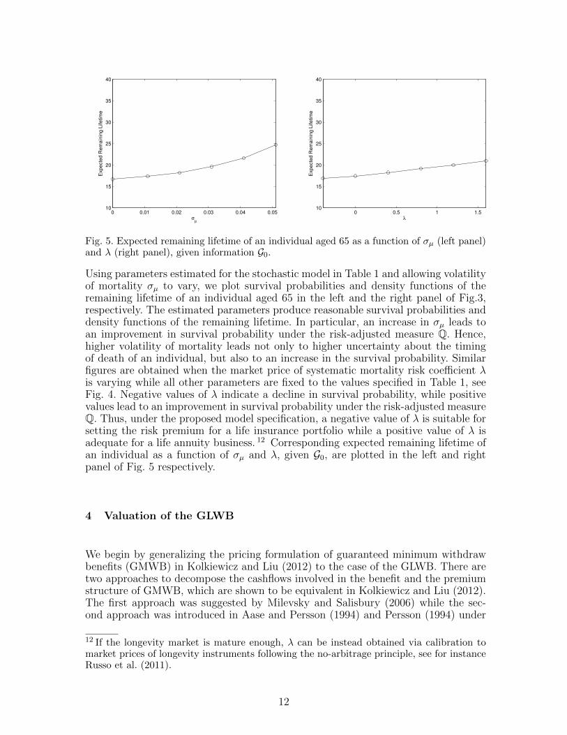
Fig. 5. Expected remaining lifetime of an individual aged 65 as a function of σµ (left panel)and λ (right panel), given information G0.
Using parameters estimated for the stochastic model in Table 1 and allowing volatilityof mortality σµ to vary, we plot survival probabilities and density functions of theremaining lifetime of an individual aged 65 in the left and the right panel of Fig.3,respectively. The estimated parameters produce reasonable survival probabilities anddensity functions of the remaining lifetime. In particular, an increase in σµ leads toan improvement in survival probability under the risk-adjusted measure Q. Hence,higher volatility of mortality leads not only to higher uncertainty about the timingof death of an individual, but also to an increase in the survival probability. Similarfigures are obtained when the market price of systematic mortality risk coefficient λis varying while all other parameters are fixed to the values specified in Table 1, seeFig. 4. Negative values of λ indicate a decline in survival probability, while positivevalues lead to an improvement in survival probability under the risk-adjusted measureQ. Thus, under the proposed model specification, a negative value of λ is suitable forsetting the risk premium for a life insurance portfolio while a positive value of λ isadequate for a life annuity business. 12 Corresponding expected remaining lifetime ofan individual as a function of σµ and λ, given G0, are plotted in the left and rightpanel of Fig. 5 respectively.
4 Valuation of the GLWB
We begin by generalizing the pricing formulation of guaranteed minimum withdrawbenefits (GMWB) in Kolkiewicz and Liu (2012) to the case of the GLWB. There aretwo approaches to decompose the cashflows involved in the benefit and the premiumstructure of GMWB, which are shown to be equivalent in Kolkiewicz and Liu (2012).The first approach was suggested by Milevsky and Salisbury (2006) while the sec-ond approach was introduced in Aase and Persson (1994) and Persson (1994) under
12 If the longevity market is mature enough, λ can be instead obtained via calibration tomarket prices of longevity instruments following the no-arbitrage principle, see for instanceRusso et al. (2011).
12

the “principle of equivalence under Q”. In the following, we present both valuationapproaches for the case of GLWB and demonstrate that these are indeed equivalentat any time t. We focus on the plain GLWB with assumptions that policyholdersexhibit static withdrawal behavior and withdrawals start immediately without anydefer period.
4.1 First Approach: Policyholder’s Perspective
Recalling the terminology above, we denote A(0) the initial investment, g the guar-anteed withdrawal rate, τ the remaining lifetime of an individual aged x at time 0,ω the maximum age allowed in the model and sPx+t the survival probability of anindividual aged x+ t at time t. From a policyholder’s perspective, income from staticwithdrawals can be regarded as an immediate life annuity. The no-arbitrage value attime t, denoted by V P
1 (t), of an immediate life annuity can be expressed as
V P1 (t) = 1τ>t gA(0)
∫ ω−x−t
0sPx+t e
−rs ds, (4.1)
where 0 ≤ t ≤ ω − x and 1τ>t denotes the indicator function taking value of one ifan individual is still alive at time t, and zero otherwise.
Let A(·) be the solution to the SDE (3.3) without the condition that A(·) is absorbedat zero. Since the account value cannot be negative and any remaining amount inthe account at the time of death of the policyholder is returned to the policyholder’sbeneficiary, this cash inflow can be regarded as a call option with payoff (A(τ))+. Bythe assumption that equity risk and systematic mortality risk are independent, wecan write the no-arbitrage value of this call option payoff at time t as
V P2 (t) = 1τ>t
∫ ω−x−t
0fx+t(s)E
Qt
(e−rs (A(t+ s))+
)ds. (4.2)
where fx+t(s) = − dds
(sPx+t) is the density function of the remaining lifetime of anindividual aged x+ t at time t.
Both, V P1 (t) and V P
2 (t) are cash inflows while the amount in the investment accountA(t) is viewed as a cash outflow to the VA provider. Under the first approach thevalue of GLWB, denoted by V P (t), is defined as
V P (t) = V P1 (t) + V P
2 (t)− 1τ>tA(t), (4.3)
which can be rewritten as
V P (t) = 1τ>t
(∫ ω−x−t
0fx+t(s)
(gA(0)
r
(1− e−rs
)+ EQ
t
(e−rs(A(t+ s))+
))ds−A(t)
),
(4.4)
where integration by parts has been applied in order to express Eq.(4.1) in termsof the remaining lifetime density fx+t(s). To make the guarantee fair to both, the
13
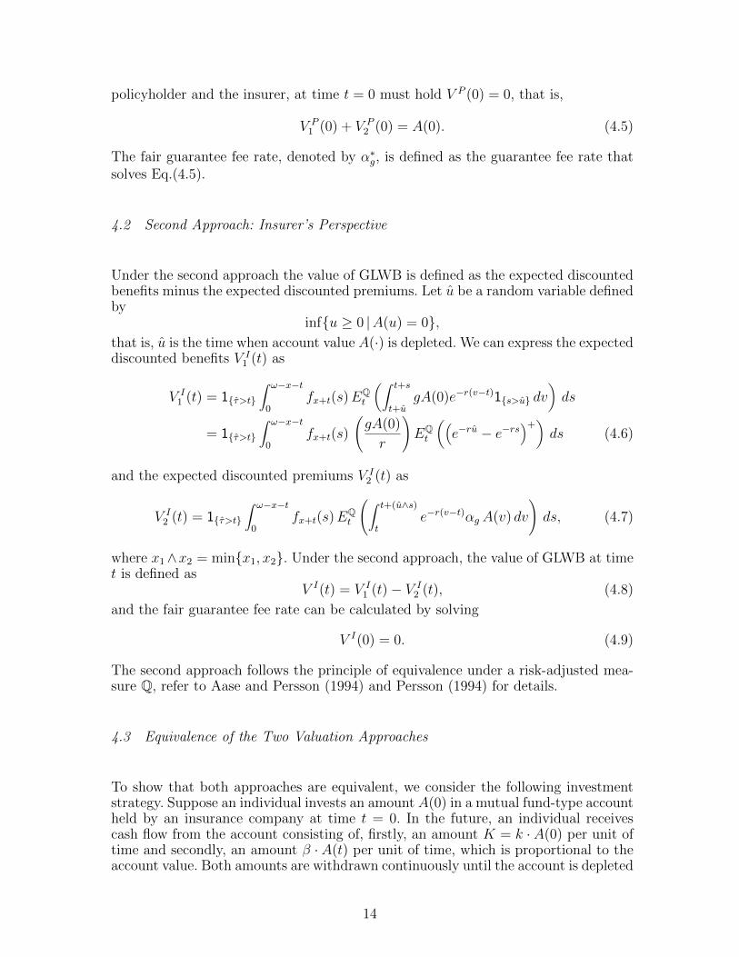
policyholder and the insurer, at time t = 0 must hold V P (0) = 0, that is,
V P1 (0) + V P
2 (0) = A(0). (4.5)
The fair guarantee fee rate, denoted by α∗g, is defined as the guarantee fee rate thatsolves Eq.(4.5).
4.2 Second Approach: Insurer’s Perspective
Under the second approach the value of GLWB is defined as the expected discountedbenefits minus the expected discounted premiums. Let u be a random variable definedby
infu ≥ 0 |A(u) = 0,that is, u is the time when account value A(·) is depleted. We can express the expecteddiscounted benefits V I
1 (t) as
V I1 (t) = 1τ>t
∫ ω−x−t
0fx+t(s)E
Qt
(∫ t+s
t+ugA(0)e−r(v−t)1s>u dv
)ds
= 1τ>t
∫ ω−x−t
0fx+t(s)
(gA(0)
r
)EQt
((e−ru − e−rs
)+)ds (4.6)
and the expected discounted premiums V I2 (t) as
V I2 (t) = 1τ>t
∫ ω−x−t
0fx+t(s)E
Qt
(∫ t+(u∧s)
te−r(v−t)αg A(v) dv
)ds, (4.7)
where x1∧x2 = minx1, x2. Under the second approach, the value of GLWB at timet is defined as
V I(t) = V I1 (t)− V I
2 (t), (4.8)
and the fair guarantee fee rate can be calculated by solving
V I(0) = 0. (4.9)
The second approach follows the principle of equivalence under a risk-adjusted mea-sure Q, refer to Aase and Persson (1994) and Persson (1994) for details.
4.3 Equivalence of the Two Valuation Approaches
To show that both approaches are equivalent, we consider the following investmentstrategy. Suppose an individual invests an amount A(0) in a mutual fund-type accountheld by an insurance company at time t = 0. In the future, an individual receivescash flow from the account consisting of, firstly, an amount K = k · A(0) per unit oftime and secondly, an amount β · A(t) per unit of time, which is proportional to theaccount value. Both amounts are withdrawn continuously until the account is depleted
14

or individual dies. Finally, any remaining amount in the account will be returned tothe individual’s beneficiary. In order to value the entire cash flow including the initialinvestment, we notice that the insurer provides no financial obligation or guaranteeto the above arrangement, that is, the role of the insurer is redundant. Thus, theno-arbitrage value of the above cash flow must be zero at time t = 0. That is, we have
EQ0
(−A(0) +
∫ u∧τ
0e−rv(K + βA(v))dv + e−rτ (A(τ))+
)= 0 (4.10)
where k ≥ 0, β ≥ 0 and A(τ) is written as (A(τ))+.
Using the fact that∫ u∧τ0 =
∫ τ0 −
∫ τu 1τ>u and rearranging the terms in Eq.(4.10), we
obtain
EQ0
(−A(0) +
∫ τ
0K e−rvdv + e−rτ (A(τ))+
)= EQ
0
(∫ τ
ue−rvK1τ>udv −
∫ u∧τ
0e−rvβA(v)dv
)(4.11)
The L.H.S. and R.H.S. of Eq.(4.11) are V P (0) and V I(0), respectively. Note that theparameter k can be interpreted as the GLWB guaranteed withdrawal rate g, whereas βis the guarantee fee rate corresponding to αg. By imposing the principle of equivalenceunder Q we note that the R.H.S. of Eq.(4.11) equals zero, which implies that theL.H.S. of Eq.(4.11) must be equal to zero as well. Since the argument does not relyon whether the remaining lifetime τ is stochastic or deterministic, it is evident thatthe equivalence holds for the valuation of GMWB where τ = T = 1/k is deterministic,assuming static withdrawal behavior. Table 2 reports in the last two columns the fairguarantee fee rate α∗g computed using the two equivalent approaches summarizedabove. The result suggests that both approaches lead to the same α∗g, subject tosimulation error with finite sample size.
Table 2Fair guarantee fees obtained using two valuation approaches. Other parameters are as
specified in Table 3.
Case r σ g σµ λ Fee (1st App.) Fee (2nd App.)1. 4% 20% 5.0% 0.04 0.2 0.48% 0.48%2. 3% 25% 4.5% 0.02 0.0 0.45% 0.45%3. 5% 15% 5.5% 0.05 0.8 0.50% 0.49%4. 4% 20% 6.0% 0.00 0.0 0.71% 0.71%
One can easily generalize Eq.(4.10) to any time t ≥ 0. Both approaches definedthrough Eq.(4.5) and Eq.(4.9) can be applied to valuate GLWB at any time t ≥ 0.
While the first approach is computationally more efficient, the second approach high-lights the theoretical result that the market reserve of a payment process is definedas the expected discounted benefit minus the expected discounted premium under arisk-adjusted measure, see Dahl and Moller (2006).
Remark 2 For some special cases the equivalence, formulated in Eq.(4.11), can beverified analytically. If A(t) follows the dynamics in SDE (3.3) and
15
(1) k = 0 and β ≥ 0, Eq.(4.11) becomes
A(0) = EQ0
(e−rτA(τ) +
∫ τ
0e−rsβA(s)ds
),
where the guarantee fee rate β can be interpreted as a continuous dividend yield,see e.g., Bjork (2009). In particular, when β = 0, it states that the discountedasset is a Q-martingale.
(2) k > 0, β = 0 and σ = 0, we have
dA(t) = (rA(t)− kA(0))dt
which has the solution
A(t) = A(0)ert +kA(0)
r
(1− ert
).
The account A(t) can be interpreted as a money market account where a constantamount is withdrawn continuously. Solving A(u) = 0 we obtain u = 1
rln k
k−r . Wecan verify Eq.(4.11) by noticing that
EQ0
(∫ u∧τ
0e−rvKdv + e−rτ (A(τ))+
)=∫ ω−x
0fx(s)
(∫ u∧s
0e−rvKdv + e−rs(A(s))+
)ds
= A(0)
where the second equality is obtained by considering two cases s ≥ u and s < useparately.
5 Sensitivity Analysis
As discussed in Section 1, risk assessment is important for analyzing the underlyingrisks of an insurance product. Given that the underlying guarantee is a long termcontract, the effect of parameter risk on pricing is expected to be significant. We usesensitivity analysis as a risk assessment to quantify the impact of parameter risk onGLWB pricing.
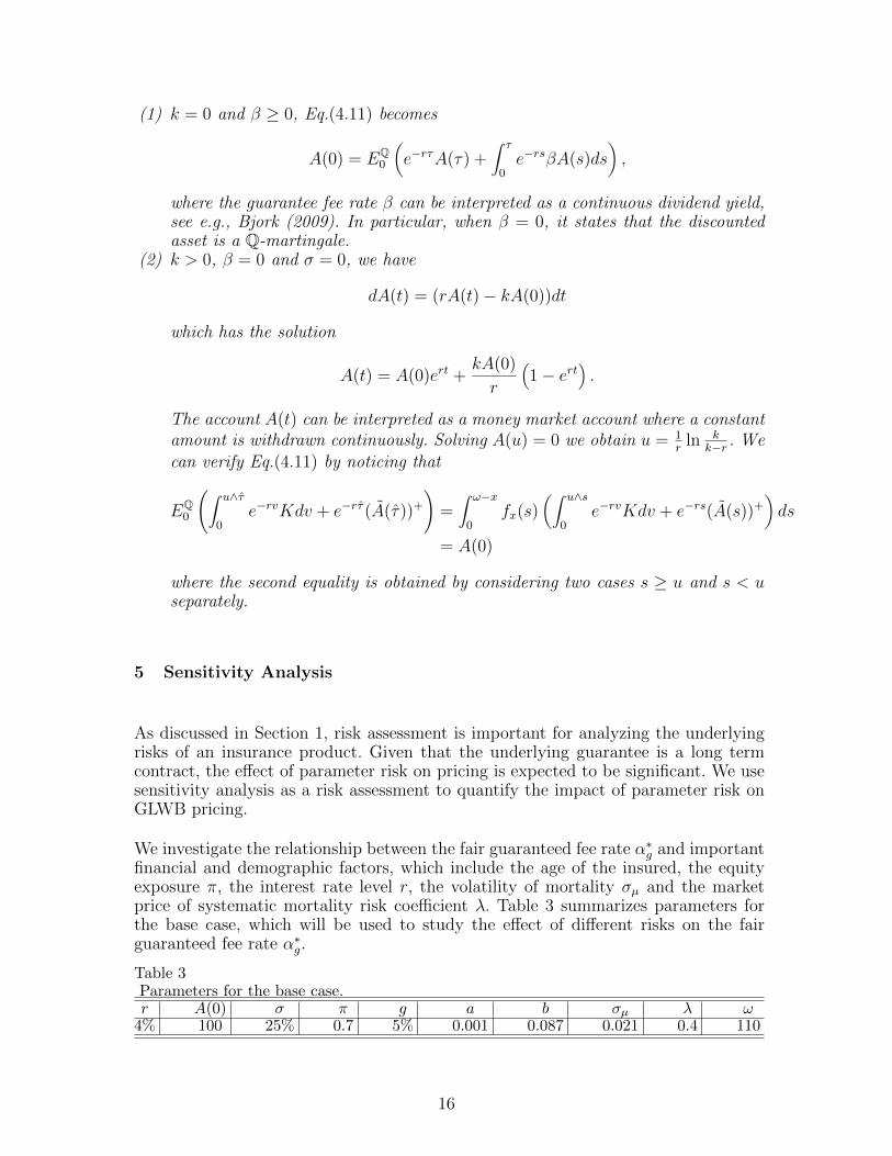
We investigate the relationship between the fair guaranteed fee rate α∗g and importantfinancial and demographic factors, which include the age of the insured, the equityexposure π, the interest rate level r, the volatility of mortality σµ and the marketprice of systematic mortality risk coefficient λ. Table 3 summarizes parameters forthe base case, which will be used to study the effect of different risks on the fairguaranteed fee rate α∗g.
Table 3Parameters for the base case.r A(0) σ π g a b σµ λ ω
4% 100 25% 0.7 5% 0.001 0.087 0.021 0.4 110
16
5.1 Sensitivity to Mortality Risk
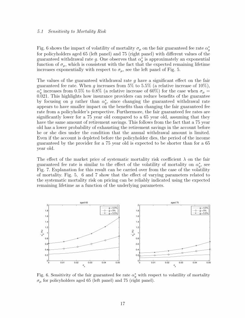
Fig. 6 shows the impact of volatility of mortality σµ on the fair guaranteed fee rate α∗gfor policyholders aged 65 (left panel) and 75 (right panel) with different values of theguaranteed withdrawal rate g. One observes that α∗g is approximately an exponentialfunction of σµ, which is consistent with the fact that the expected remaining lifetimeincreases exponentially with respect to σµ, see the left panel of Fig. 5.
The values of the guaranteed withdrawal rate g have a significant effect on the fairguaranteed fee rate. When g increases from 5% to 5.5% (a relative increase of 10%),α∗g increases from 0.5% to 0.8% (a relative increase of 60%) for the case when σµ =0.021. This highlights how insurance providers can reduce benefits of the guaranteeby focusing on g rather than α∗g, since changing the guaranteed withdrawal rateappears to have smaller impact on the benefits than changing the fair guaranteed feerate from a policyholder’s perspective. Furthermore, the fair guaranteed fee rates aresignificantly lower for a 75 year old compared to a 65 year old, assuming that theyhave the same amount of retirement savings. This follows from the fact that a 75 yearold has a lower probability of exhausting the retirement savings in the account beforehe or she dies under the condition that the annual withdrawal amount is limited.Even if the account is depleted before the policyholder dies, the period of the incomeguaranteed by the provider for a 75 year old is expected to be shorter than for a 65year old.
The effect of the market price of systematic mortality risk coefficient λ on the fairguaranteed fee rate is similar to the effect of the volatility of mortality on α∗g, seeFig. 7. Explanation for this result can be carried over from the case of the volatilityof mortality. Fig. 5, 6 and 7 show that the effect of varying parameters related tothe systematic mortality risk on pricing can be reliably indicated using the expectedremaining lifetime as a function of the underlying parameters.
0 0.01 0.02 0.03 0.04 0.050
0.2
0.4
0.6
0.8
1
1.2
1.4
1.6
1.8
2
σµ
α* g (
%)
aged 65
g = 4.5%
g = 5%
g = 5.5%
0 0.01 0.02 0.03 0.04 0.050
0.2
0.4
0.6
0.8
1
1.2
1.4
1.6
1.8
2
σµ
α* g (
%)
aged 75
g = 4.5%
g = 5%
g = 5.5%
Fig. 6. Sensitivity of the fair guaranteed fee rate α∗g with respect to volatility of mortalityσµ for policyholders aged 65 (left panel) and 75 (right panel).
17
0 0.5 1 1.50
0.2
0.4
0.6
0.8
1
1.2
1.4
1.6
1.8
2
λ
α* g (
%)
aged 65
g = 4.5%
g = 5%
g = 5.5%
0 0.5 1 1.50
0.2
0.4
0.6
0.8
1
1.2
1.4
1.6
1.8
2
λ
α* g (
%)
aged 75
g = 4.5%
g = 5%
g = 5.5%
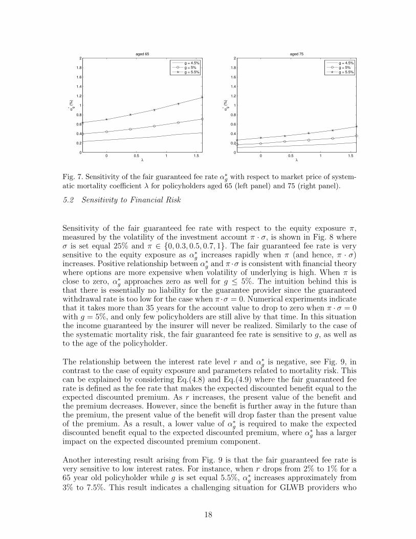
Fig. 7. Sensitivity of the fair guaranteed fee rate α∗g with respect to market price of system-atic mortality coefficient λ for policyholders aged 65 (left panel) and 75 (right panel).
5.2 Sensitivity to Financial Risk
Sensitivity of the fair guaranteed fee rate with respect to the equity exposure π,measured by the volatility of the investment account π · σ, is shown in Fig. 8 whereσ is set equal 25% and π ∈ 0, 0.3, 0.5, 0.7, 1. The fair guaranteed fee rate is verysensitive to the equity exposure as α∗g increases rapidly when π (and hence, π · σ)increases. Positive relationship between α∗g and π ·σ is consistent with financial theorywhere options are more expensive when volatility of underlying is high. When π isclose to zero, α∗g approaches zero as well for g ≤ 5%. The intuition behind this isthat there is essentially no liability for the guarantee provider since the guaranteedwithdrawal rate is too low for the case when π ·σ = 0. Numerical experiments indicatethat it takes more than 35 years for the account value to drop to zero when π · σ = 0with g = 5%, and only few policyholders are still alive by that time. In this situationthe income guaranteed by the insurer will never be realized. Similarly to the case ofthe systematic mortality risk, the fair guaranteed fee rate is sensitive to g, as well asto the age of the policyholder.
The relationship between the interest rate level r and α∗g is negative, see Fig. 9, incontrast to the case of equity exposure and parameters related to mortality risk. Thiscan be explained by considering Eq.(4.8) and Eq.(4.9) where the fair guaranteed feerate is defined as the fee rate that makes the expected discounted benefit equal to theexpected discounted premium. As r increases, the present value of the benefit andthe premium decreases. However, since the benefit is further away in the future thanthe premium, the present value of the benefit will drop faster than the present valueof the premium. As a result, a lower value of α∗g is required to make the expecteddiscounted benefit equal to the expected discounted premium, where α∗g has a largerimpact on the expected discounted premium component.
Another interesting result arising from Fig. 9 is that the fair guaranteed fee rate isvery sensitive to low interest rates. For instance, when r drops from 2% to 1% for a65 year old policyholder while g is set equal 5.5%, α∗g increases approximately from3% to 7.5%. This result indicates a challenging situation for GLWB providers who
18
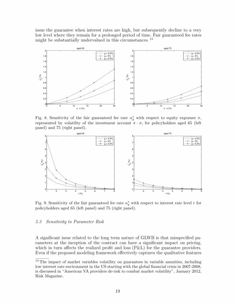
issue the guarantee when interest rates are high, but subsequently decline to a verylow level where they remain for a prolonged period of time. Fair guaranteed fee ratesmight be substantially undervalued in this circumstances. 13
0 5 10 15 20 250
0.2
0.4
0.6
0.8
1
1.2
1.4
1.6
1.8
2
π ⋅ σ (%)
α* g (
%)
aged 65
g = 4.5%
g = 5%
g = 5.5%
0 5 10 15 20 250
0.2
0.4
0.6
0.8
1
1.2
1.4
1.6
1.8
2
π ⋅ σ (%)
α* g (
%)
aged 75
g = 4.5%
g = 5%
g = 5.5%
Fig. 8. Sensitivity of the fair guaranteed fee rate α∗g with respect to equity exposure π,represented by volatility of the investment account π · σ, for policyholders aged 65 (leftpanel) and 75 (right panel).
1 2 3 4 5 6 7 80
1
2
3
4
5
6
7
8
r (%)
α* g (
%)
aged 65
g = 4.5%
g = 5%
g = 5.5%
1 2 3 4 5 6 7 80
1
2
3
4
5
6
7
8
r (%)
α* g (
%)
aged 75
g = 4.5%
g = 5%
g = 5.5%
Fig. 9. Sensitivity of the fair guaranteed fee rate α∗g with respect to interest rate level r forpolicyholders aged 65 (left panel) and 75 (right panel).
5.3 Sensitivity to Parameter Risk
A significant issue related to the long term nature of GLWB is that misspecified pa-rameters at the inception of the contract can have a significant impact on pricing,which in turn affects the realized profit and loss (P&L) for the guarantee providers.Even if the proposed modeling framework effectively captures the qualitative features
13 The impact of market variables volatility on guarantees in variable annuities, includinglow interest rate environment in the US starting with the global financial crisis in 2007-2008,is discussed in “American VA providers de-risk to combat market volatility”, January 2012,Risk Magazine.
19
of the underlying financial and demographic variables, estimation of model param-eters is a challenging task. The challenge arises partly due to the fact that marketsfor the long term contracts are relatively illiquid, and hence no reliable market pricesare available for parameter calibration. However, one could rely on historical data,perhaps combined with expert judgements, when estimating parameters and pricinga long term contract. Given the long term nature of the guarantee, perfect hedgingis economically unviable when taking transaction costs and liquidity into account. Inthese circumstances the insurance provider must accept a certain level of parameterrisk. Sensitivity analysis of the relative impact of these risks inherent in parameter(mis)specification on pricing of the guarantee is an important step towards under-standing the risks undertaken by the guarantee providers.
In the following we study the impact of different model parameters on pricing ofGLWB. As shown in Fig. 9, the fair guaranteed fee rate is extremely sensitive tolow interest rates. The level of interest rates is important when pricing GLWB, espe-cially in a prolonged period of low interest rate environment. Fig. 6 and Fig. 8 showhow equity exposure π, and hence volatility of the investment account π · σ, have alarger impact on pricing of GLWB than the volatility of mortality σµ. However, theparameter risk of σµ is non-negligible, which is illustrated by considering the follow-ing scenario. Suppose that the volatility of mortality σµ = 0.02 is fixed (all otherparameters are as specified in Table 3) and the guarantee provider estimates fund’svolatility to be σ = 20% at the time when the guarantee is issued. However, it turnsout in the future that the “true” parameter corresponds to σ = 25%. In this scenariothe guarantee provider has misspecified σ by 5%. This leads to an underestimationof the guaranteed fee rate α∗g by approx. (0.6− 0.4)% = 0.2%, see Fig. 8 (for the caseg = 5%). On the other hand, the same magnitude of mis(pricing) of α∗g (0.2%) canbe observed when σ = 25% is fixed while the volatility of mortality σµ is misspecifiedby approximately (0.04 − 0.02) = 0.02 (if the original estimation of σµ were 0.02at the inception of the guarantee while the “true” parameter value turns out to beσµ = 0.04 in the future), see Fig. 6 (for the case g = 5%). If volatility of mortalitychanges from σµ = 0.02 to σµ = 0.04, the expected remaining lifetime would increaseby approximately (21− 18) = 3 years, see Fig. 5. An underestimation of three yearsof expected remaining lifetime for a period of 30 to 40 years 14 is possible and therisk of misspecification of the volatility of mortality cannot be ignored.
6 Profit and Loss Analysis
Although sensitivity analysis provides us with a quantitative measure for the degreeof impact of parameter risk on pricing, profit and loss (P&L) analysis can provideanother perspective especially when hedging is not available or difficult to carry out.Hari et al. (2008) use P&L analysis to assess systematic mortality risk in pensionannuities.
In order to better assess the underlying risks involved in GLWB, we simulate profit
14 This corresponds approximately to the duration of a VA portfolio with GLWB.
20
and loss (P&L) distributions for different scenarios where no hedging is performed andliabilities are funded solely by the guaranteed fee charged by the insurer. We assumethat the VA portfolio consists of 1000 policyholders all aged 65 who have electedGLWB as the only guarantee to protect their investment. Each individual invests$100 and chooses the same equity exposure π for their retirement savings investment.A fair guaranteed fee is charged according to the valuation result in Section 4.
The P&L for each individual is obtained by simulating the account process A(·). Ifpolicyholder dies before the account is depleted, the profit for the insurer is determinedby the received fee, which grows at an interest rate r. On the other hand, if policy-holder dies after the account value is depleted, the fee charged by the insurer will beused to fund incurred liabilities. We simulate the mortality intensity process µ65+t foreach scenario and apply the inverse transform method (Brigo and Mercurio (2006)) towe obtain 1,000 independent remaining lifetimes. The surplus/shortfall is aggregatedacross all individuals, divided by the total investment (1, 000 · $100 = $100, 000), anddiscounted to obtain the discounted P&L of the portfolio per dollar received. 15 Thedescribed procedure constitutes one sample. To obtain summary statistics for thediscounted P&L distribution, 100,000 simulations are performed.
Summary statistics for the discounted P&L distributions include the fair guaranteedfee rate α∗g; the mean P&L for the insurer; its standard deviation; the coefficient ofvariation (C.V.) defined as the ratio of standard deviation over the the mean P&L;the Value-at-Risk (VaR) defined as the q%-quantile of the P&L distribution; and theExpected Shortfall (ES) determined as the expected loss of the portfolio given thatthe loss occurs at or below the q%-quantile. The confidence level for the VaR and theES corresponds to 99.5%. Parameter values used in the simulations are as specifiedin Table 3 except for the guaranteed withdrawal rate g which is set equal to 6%. 16
6.1 P&L with or without systematic mortality risk
We first consider interaction between systematic mortality risk and equity exposureπ, and its effect on the P&L. Table 4 reports summary statistics for the discountedP&L distributions with systematic mortality risk (with s.m.r) or without systematicmortality risk (no s.m.r.). We first consider the situation when π = 0, that is, theretirement savings is entirely invested in the money market account with deterministicgrowth. Since portfolio is large enough, the unsystematic mortality risk is diversifiedaway. When π = 0 and there is no s.m.r., the fee charged by the insurer is able toalmost exactly (on average) offset the liability.
15 Since the time of death of a policyholder is random and the maturity of the contract isnot fixed, using discounted P&L rather than P&L allows for a more convenient comparisonand interpretation of the results at time t = 0.16 When equity exposure π = 0, the guarantee is too generous for the insurer. This leads topositive VaR and ES even for a relatively high confidence level 99.5%. For the purpose ofconvenience of interpretation of the results, we increase g from 5% to 6%, which leads tonegative VaR and ES across all equity exposures.
21
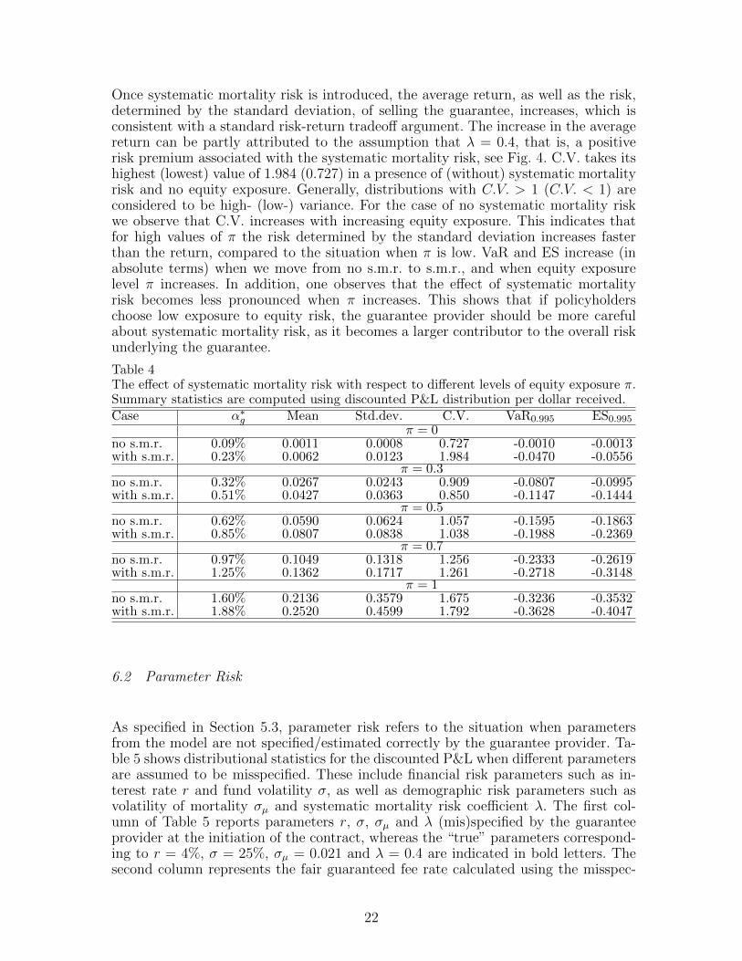
Once systematic mortality risk is introduced, the average return, as well as the risk,determined by the standard deviation, of selling the guarantee, increases, which isconsistent with a standard risk-return tradeoff argument. The increase in the averagereturn can be partly attributed to the assumption that λ = 0.4, that is, a positiverisk premium associated with the systematic mortality risk, see Fig. 4. C.V. takes itshighest (lowest) value of 1.984 (0.727) in a presence of (without) systematic mortalityrisk and no equity exposure. Generally, distributions with C.V. > 1 (C.V. < 1) areconsidered to be high- (low-) variance. For the case of no systematic mortality riskwe observe that C.V. increases with increasing equity exposure. This indicates thatfor high values of π the risk determined by the standard deviation increases fasterthan the return, compared to the situation when π is low. VaR and ES increase (inabsolute terms) when we move from no s.m.r. to s.m.r., and when equity exposurelevel π increases. In addition, one observes that the effect of systematic mortalityrisk becomes less pronounced when π increases. This shows that if policyholderschoose low exposure to equity risk, the guarantee provider should be more carefulabout systematic mortality risk, as it becomes a larger contributor to the overall riskunderlying the guarantee.
Table 4The effect of systematic mortality risk with respect to different levels of equity exposure π.Summary statistics are computed using discounted P&L distribution per dollar received.Case α∗g Mean Std.dev. C.V. VaR0.995 ES0.995
π = 0no s.m.r. 0.09% 0.0011 0.0008 0.727 -0.0010 -0.0013with s.m.r. 0.23% 0.0062 0.0123 1.984 -0.0470 -0.0556
π = 0.3no s.m.r. 0.32% 0.0267 0.0243 0.909 -0.0807 -0.0995with s.m.r. 0.51% 0.0427 0.0363 0.850 -0.1147 -0.1444
π = 0.5no s.m.r. 0.62% 0.0590 0.0624 1.057 -0.1595 -0.1863with s.m.r. 0.85% 0.0807 0.0838 1.038 -0.1988 -0.2369
π = 0.7no s.m.r. 0.97% 0.1049 0.1318 1.256 -0.2333 -0.2619with s.m.r. 1.25% 0.1362 0.1717 1.261 -0.2718 -0.3148
π = 1no s.m.r. 1.60% 0.2136 0.3579 1.675 -0.3236 -0.3532with s.m.r. 1.88% 0.2520 0.4599 1.792 -0.3628 -0.4047
6.2 Parameter Risk
As specified in Section 5.3, parameter risk refers to the situation when parametersfrom the model are not specified/estimated correctly by the guarantee provider. Ta-ble 5 shows distributional statistics for the discounted P&L when different parametersare assumed to be misspecified. These include financial risk parameters such as in-terest rate r and fund volatility σ, as well as demographic risk parameters such asvolatility of mortality σµ and systematic mortality risk coefficient λ. The first col-umn of Table 5 reports parameters r, σ, σµ and λ (mis)specified by the guaranteeprovider at the initiation of the contract, whereas the “true” parameters correspond-ing to r = 4%, σ = 25%, σµ = 0.021 and λ = 0.4 are indicated in bold letters. Thesecond column represents the fair guaranteed fee rate calculated using the misspec-
22
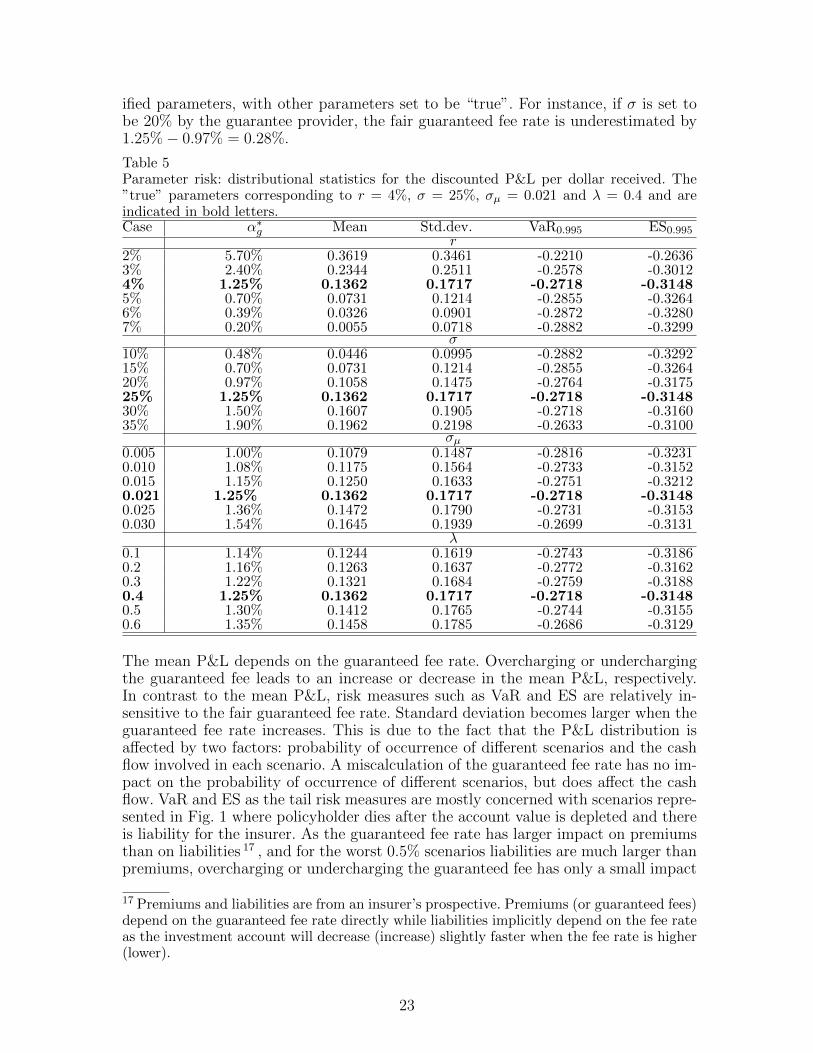
ified parameters, with other parameters set to be “true”. For instance, if σ is set tobe 20% by the guarantee provider, the fair guaranteed fee rate is underestimated by1.25%− 0.97% = 0.28%.
Table 5Parameter risk: distributional statistics for the discounted P&L per dollar received. The”true” parameters corresponding to r = 4%, σ = 25%, σµ = 0.021 and λ = 0.4 and areindicated in bold letters.Case α∗g Mean Std.dev. VaR0.995 ES0.995
r2% 5.70% 0.3619 0.3461 -0.2210 -0.26363% 2.40% 0.2344 0.2511 -0.2578 -0.30124% 1.25% 0.1362 0.1717 -0.2718 -0.31485% 0.70% 0.0731 0.1214 -0.2855 -0.32646% 0.39% 0.0326 0.0901 -0.2872 -0.32807% 0.20% 0.0055 0.0718 -0.2882 -0.3299
σ10% 0.48% 0.0446 0.0995 -0.2882 -0.329215% 0.70% 0.0731 0.1214 -0.2855 -0.326420% 0.97% 0.1058 0.1475 -0.2764 -0.317525% 1.25% 0.1362 0.1717 -0.2718 -0.314830% 1.50% 0.1607 0.1905 -0.2718 -0.316035% 1.90% 0.1962 0.2198 -0.2633 -0.3100
σµ0.005 1.00% 0.1079 0.1487 -0.2816 -0.32310.010 1.08% 0.1175 0.1564 -0.2733 -0.31520.015 1.15% 0.1250 0.1633 -0.2751 -0.32120.021 1.25% 0.1362 0.1717 -0.2718 -0.31480.025 1.36% 0.1472 0.1790 -0.2731 -0.31530.030 1.54% 0.1645 0.1939 -0.2699 -0.3131
λ0.1 1.14% 0.1244 0.1619 -0.2743 -0.31860.2 1.16% 0.1263 0.1637 -0.2772 -0.31620.3 1.22% 0.1321 0.1684 -0.2759 -0.31880.4 1.25% 0.1362 0.1717 -0.2718 -0.31480.5 1.30% 0.1412 0.1765 -0.2744 -0.31550.6 1.35% 0.1458 0.1785 -0.2686 -0.3129
The mean P&L depends on the guaranteed fee rate. Overcharging or underchargingthe guaranteed fee leads to an increase or decrease in the mean P&L, respectively.In contrast to the mean P&L, risk measures such as VaR and ES are relatively in-sensitive to the fair guaranteed fee rate. Standard deviation becomes larger when theguaranteed fee rate increases. This is due to the fact that the P&L distribution isaffected by two factors: probability of occurrence of different scenarios and the cashflow involved in each scenario. A miscalculation of the guaranteed fee rate has no im-pact on the probability of occurrence of different scenarios, but does affect the cashflow. VaR and ES as the tail risk measures are mostly concerned with scenarios repre-sented in Fig. 1 where policyholder dies after the account value is depleted and thereis liability for the insurer. As the guaranteed fee rate has larger impact on premiumsthan on liabilities 17 , and for the worst 0.5% scenarios liabilities are much larger thanpremiums, overcharging or undercharging the guaranteed fee has only a small impact
17 Premiums and liabilities are from an insurer’s prospective. Premiums (or guaranteed fees)depend on the guaranteed fee rate directly while liabilities implicitly depend on the fee rateas the investment account will decrease (increase) slightly faster when the fee rate is higher(lower).
23
on the low tail of the P&L distribution. As a result, VaR and ES are relatively robustto miss-specification of the guaranteed fee rate.
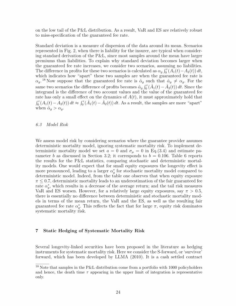
Standard deviation is a measure of dispersion of the data around its mean. Scenariosrepresented in Fig. 2, when there is liability for the insurer, are typical when consider-ing standard derivation of the P&L, since most samples around the mean have largerpremiums than liabilities. To explain why standard deviation becomes larger whenthe guaranteed fee rate increases, we consider two scenarios, assuming no liabilities.The difference in profits for these two scenarios is calculated as αg
∫ τ0 (A1(t)−A2(t)) dt,
which indicates how “apart” these two samples are when the guaranteed fee rate isαg.
18 Now suppose that the guaranteed fee rate is αg such that αg 6= αg. For the
same two scenarios the difference of profits becomes αg∫ τ0 (A1(t)− A2(t)) dt. Since the
integrand is the difference of two account values and the value of the guaranteed feerate has only a small effect on the dynamics of A(t), it must approximately hold that∫ τ0 (A1(t)−A2(t)) dt ≈
∫ τ0 (A1(t)− A2(t)) dt. As a result, the samples are more “apart”
when αg > αg.
6.3 Model Risk
We assess model risk by considering scenarios where the guarantee provider assumesdeterministic mortality model, ignoring systematic mortality risk. To implement de-terministic mortality model we set a = 0 and σµ = 0 in Eq.(3.4) and estimate pa-rameter b as discussed in Section 3.2; it corresponds to b = 0.106. Table 6 reportsthe results for the P&L statistics, comparing stochastic and deterministic mortal-ity models. One would expect that for small equity exposures the longevity effect ismore pronounced, leading to a larger α∗g for stochastic mortality model compared todeterministic model. Indeed, from the table one observes that when equity exposureπ ≤ 0.7, deterministic mortality leads to an underestimation of the fair guaranteed feerate α∗g, which results in a decrease of the average return; and the tail risk measuresVaR and ES worsen. However, for a relatively large equity exposures, say π > 0.5,there is essentially no difference between deterministic and stochastic mortality mod-els in terms of the mean return, the VaR and the ES, as well as the resulting fairguaranteed fee rate α∗g. This reflects the fact that for large π, equity risk dominatessystematic mortality risk.
7 Static Hedging of Systematic Mortality Risk
Several longevity-linked securities have been proposed in the literature as hedginginstruments for systematic mortality risk. Here we consider the S-forward, or ‘survivor’forward, which has been developed by LLMA (2010). It is a cash settled contract
18 Note that samples in the P&L distribution come from a portfolio with 1000 policyholdersand hence, the death time τ appearing in the upper limit of integration is representativeonly.
24

Table 6Model risk assuming stochastic vs. deterministic mortality model: distributional statisticsfor the discounted P&L per dollar received.Model α∗g Mean Std.dev. VaR0.995 ES0.995
π = 0stochastic 0.23% 0.0062 0.0123 -0.0470 -0.0556deterministic 0.14% 0.0001 0.0114 -0.0501 -0.0581
π = 0.3stochastic 0.50% 0.0427 0.0363 -0.1147 -0.1444deterministic 0.44% 0.0371 0.0345 -0.1166 -0.1507
π = 0.5stochastic 0.85% 0.0807 0.0838 -0.1988 -0.2369deterministic 0.81% 0.0772 0.0822 -0.2026 -0.2408
π = 0.7stochastic 1.25% 0.1362 0.1717 -0.2718 -0.3148deterministic 1.23% 0.1326 0.1685 -0.2731 -0.3174
π = 1stochastic 1.88% 0.2520 0.4599 -0.3628 -0.4047deterministic 1.90% 0.2534 0.4478 -0.3684 -0.4117
linked to survival rates of a given population cohort. The S-forward is the basicbuilding block for longevity (survivor) swaps, see Dowd (2003), which are used bypension funds and insurance companies to hedge their longevity risk. Longevity swapscan be regarded as a stream of S-forwards with different maturity dates. The S-forwardis an agreement between two counterparties to exchange at maturity an amount equalto the realized survival rate of a given population cohort, with that of a fixed survivalrate agreed at the inception of the contract.
One of the advantages of using S-forwards as our choice of hedging strategy is thatthere is no initial capital requirement at the inception of the contract and cash flowsoccur only at maturity. This is in line with our P&L analysis. Another benefit of us-ing S-forward is that the underlying of the contract is the survival probability whichhas a closed form analytical expression under the proposed continuous time mortalitymodelling framework. Since dynamic hedging requires liquid longevity-linked instru-ments and the longevity market is illiquid, the choice of using static hedging is morerealistic.
An S-forward is a swap with only one payment at maturity T where the fixed legpays an amount equal to
N · EQ0
(e−∫ T0µx+s(s)ds
)(7.1)
while the floating leg pays an amount
N · e−∫ T0µx+s(s)ds, (7.2)
with N denoting the notional amount of the contract. The fixed leg is determinedunder the risk-adjusted measure Q which is discussed in Section 3.3. Given that thereis a positive risk premium for systematic mortality risk, mortality risk hedger whopays fixed leg and receives floating leg bears implicit cost for entering the S-forward.
Since maturity of the GLWB is not fixed, our numerical example assumes T = 20,which approximately corresponds to the expected remaining lifetime of a 65 year old
25
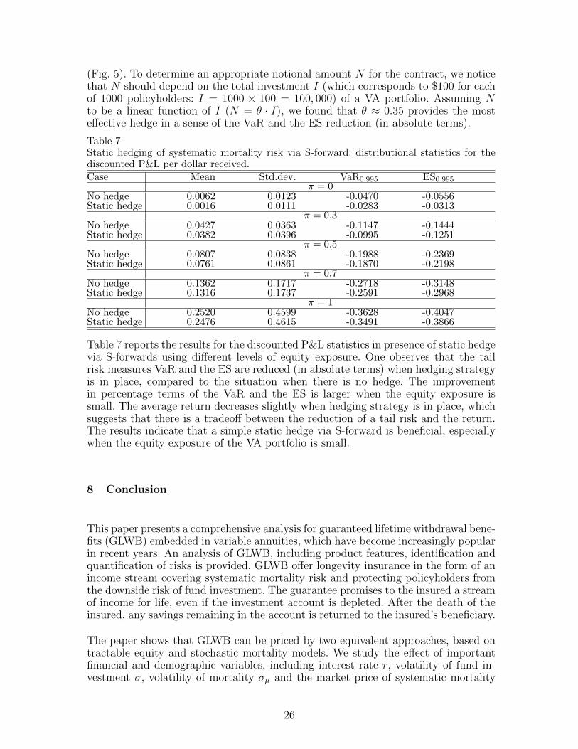
(Fig. 5). To determine an appropriate notional amount N for the contract, we noticethat N should depend on the total investment I (which corresponds to $100 for eachof 1000 policyholders: I = 1000 × 100 = 100, 000) of a VA portfolio. Assuming Nto be a linear function of I (N = θ · I), we found that θ ≈ 0.35 provides the mosteffective hedge in a sense of the VaR and the ES reduction (in absolute terms).
Table 7Static hedging of systematic mortality risk via S-forward: distributional statistics for thediscounted P&L per dollar received.Case Mean Std.dev. VaR0.995 ES0.995
π = 0No hedge 0.0062 0.0123 -0.0470 -0.0556Static hedge 0.0016 0.0111 -0.0283 -0.0313
π = 0.3No hedge 0.0427 0.0363 -0.1147 -0.1444Static hedge 0.0382 0.0396 -0.0995 -0.1251
π = 0.5No hedge 0.0807 0.0838 -0.1988 -0.2369Static hedge 0.0761 0.0861 -0.1870 -0.2198
π = 0.7No hedge 0.1362 0.1717 -0.2718 -0.3148Static hedge 0.1316 0.1737 -0.2591 -0.2968
π = 1No hedge 0.2520 0.4599 -0.3628 -0.4047Static hedge 0.2476 0.4615 -0.3491 -0.3866
Table 7 reports the results for the discounted P&L statistics in presence of static hedgevia S-forwards using different levels of equity exposure. One observes that the tailrisk measures VaR and the ES are reduced (in absolute terms) when hedging strategyis in place, compared to the situation when there is no hedge. The improvementin percentage terms of the VaR and the ES is larger when the equity exposure issmall. The average return decreases slightly when hedging strategy is in place, whichsuggests that there is a tradeoff between the reduction of a tail risk and the return.The results indicate that a simple static hedge via S-forward is beneficial, especiallywhen the equity exposure of the VA portfolio is small.
8 Conclusion
This paper presents a comprehensive analysis for guaranteed lifetime withdrawal bene-fits (GLWB) embedded in variable annuities, which have become increasingly popularin recent years. An analysis of GLWB, including product features, identification andquantification of risks is provided. GLWB offer longevity insurance in the form of anincome stream covering systematic mortality risk and protecting policyholders fromthe downside risk of fund investment. The guarantee promises to the insured a streamof income for life, even if the investment account is depleted. After the death of theinsured, any savings remaining in the account is returned to the insured’s beneficiary.
The paper shows that GLWB can be priced by two equivalent approaches, based ontractable equity and stochastic mortality models. We study the effect of importantfinancial and demographic variables, including interest rate r, volatility of fund in-vestment σ, volatility of mortality σµ and the market price of systematic mortality
26
risk λ, on the fair guaranteed fee rate α∗g charged by the insurer, as well as on theprofit and loss characteristics from the point of view of the insurance provider.
The results show that the fair guaranteed fee rate increases with increasing volatility ofmortality σµ and the market price of systematic mortality risk λ. The fair guaranteedfee rate is also positively related, and highly sensitive to, the equity exposure (hencevolatility) of the investment account. The relationship between α∗g and interest rater is negative and α∗g is highly sensitive to low interest rates.
Quantification and assessment of risks underlying GLWB is studied via P&L distri-butions, assuming no hedging in place. Tail risk measures such as the Value-at-Risk(VaR) and the Expected Shortfall (ES) are higher when systematic mortality risk ispresent in the model, compared to the situation with no systematic mortality risk.We quantify parameter risk and model risk, showing how these risks could resultin significant under- or over-estimation of the fair guaranteed fee rate α∗g. Finally, astatic hedging strategy implemented using S-forwards results in the reduction of theVaR and the ES numbers, but also leads to a decrease in the average return for theguarantee provider, especially for low levels of equity exposure. We demonstrate inthe paper that while financial risk is substantial for GLWB, the impact of systematicmortality risk on the guarantee cannot be ignored.
Acknowledgement: Fung acknowledges the Australian Postgraduate Award schol-arship and financial support from the Australian School of Business, UNSW. Ignatievaacknowledges financial support from the Australian School of Business, UNSW. Sher-ris acknowledges the support of the Australian Research Council Centre of Excellencein Population and Ageing Research (project number CE110001029).
References
Aase, K. K., Persson, S. A., 1994. Pricing of unit-linked life insurance policies. Scan-dinavian Actuarial Journal 1, 26–52.
Bacinello, A. R., Millossovich, P., Olivieri, A., Pitacco, E., 2011. Variable annuities: Aunifying valuation approach. Insurance: Mathematics and Economics 49, 285–297.
Ballotta, L., Haberman, S., 2006. The fair valuation problem of guaranteed annuityoptions: the stochastic mortality environment case. Insurance: Mathematics andEconomics 38, 195–214.
Biffis, E., 2005. Affine processes for dynamics mortality and actuarial valuations.Insurance: Mathematics and Economics 37(3), 443–468.
Bjork, T., 2009. Arbitrage Theory in Continuous Time. Oxford University Press.Brigo, D., Mercurio, F., 2006. Interest Rate Models - Theory and Practice, 2nd Edi-
tion. Springer.Cairns, A., Blake, D., Dowd, K., 2006. Pricing death: Framework for the valuation
and securitization of mortality risk. ASTIN Bulletin 36(1), 79–120.Cairns, A., Blake, D., Dowd, K., 2008. Modelling and management of mortality risk:
a review. Scandinavian Actuarial Journal 2(3), 79–113.Dahl, M., Moller, T., 2006. Valuation and hedging of life insurance liabilities with
systematic mortality risk. Insurance: Mathematics and Economics 39, 193–217.Dowd, K., 2003. Survivor bonds: A comment on blake and burrows. Journal of Risk
and Insurance 70(2), 339–348.Filipovic, D., 2009. Term Structure Models: A Graduate Course. Springer.
27
Hardy, M., 2003. Investment guarantees: The new science of modelling and risk man-agement for equity-linked life insurance. John Wiley & Sons, Inc., Hoboken, NewJersey, 2003.
Hari, N., Waegenaere, A., Melenberg, B., Nijman, T., 2008. Longevity risk in portfolioof pension annuities. Insurance: Mathematics and Economics 42, 505–519.
Holz, D., Kling, A., Rub, J., 2007. An analysis of lifelong withdrawal guarantees.Working paper, ULM University.
Kling, A., Ruez, F., Russ, J., 2011. The impact of stochastic volatility on pricing,hedging and hedge effectiveness of withdrawal benefit guarantees in variable annu-ities. ASTIN Bulletin 41 (2), 511–545.
Kling, A., Russ, J., Schilling, K., 2012. Risk analysis of annuity conversion options ina stochastic mortality environment. Tech. rep., working paper.
Kolkiewicz, A., Liu, Y., 2012. Semi-static hedging for GMWB in variable annuities.North American Actuarial Journal 16 (1), 112–140.
Ledlie, M., Corry, D., Finkelstein, G., Ritchie, A., Su, K., Wilson, D., 2008. Variableannuities. British Actuarial Journal 14, 327–389.
LLMA, 2010. Technical note: The S-forward.Luciano, E., Vigna, E., 2008. Mortality risk via affine stochastic intensities: calibration
and empirical relevance. Belgian Actuarial Bulletin 8(1), 5–16.Milevsky, M., Salisbury, T., 2006. Financial valuation of guaranteed minimum with-
drawal benefits. Insurance: Mathematics and Economics 38, 21–38.Ngai, A., Sherris, M., 2011. Longevity risk management for life and variable annuities:
the effectiveness of static hedging using longevity bonds and derivatives. Insurance:Mathematics and Economics 49, 100–114.
Persson, S. A., 1994. Stochastic interest rate in life insurance: The principle of equiv-alence revisited. Scandinavian Actuarial Journal 2, 97–112.
Piscopo, G., Haberman, S., 2011. The valuation of guaranteed lifelong withdrawalbenefit options in variable annuity contracts and the impact of mortality risk.North American Actuarial Journal 15 (1), 59–76.
Russo, V., Giacometti, R., Ortobelli, S., Rachev, S., Fabozzi, F., 2011. Calibrat-ing affine stochastic mortality models using term assurance premiums. Insurance:mathematics and economics 49, 53–60.
Schrager, D., 2006. Affine stochastic mortality. Insurance: Mathematics and Eco-nomics 38, 81–97.
Ziveyi, J., Blackburn, C., Sherris, M., 2013. Pricing European options on deferredannuities. Insurance: Mathematics and Economics 52(2), 300–311.
28