Embed Size (px)
Citation preview
Department of Civil and Environmental Engineering University College Cork (UCC)
Ireland
Systematic Framework for Selection, Use and Optimisation of Building Energy Simulation Software for a Hybrid Mechanical System
By
Ross J. McCarthy, BEng (Building Services) M.I.E.I
Supervisor: Dr. Marcus Keane A Minor Research Thesis submitted to National University of Ireland,
Cork in candidature for the degree of Master of Sustainable Energy

Systematic Framework for Selection, Use and Optimisation of Building Energy Simulation for a Hybrid Mechanical System
MEngSc Minor Thesis CE5002 Ross McCarthy 2
September 2007
Table of Contents
1 Introduction ................................................................................................................... 4
1.1 General ................................................................................................................... 4 1.2 Research Objective ................................................................................................. 5 1.3 Project Scope ................................................................................................................ 6 1.4 Buildings Current energy use ....................................................................................... 6
2 Simulation Software Selection ...................................................................................... 7
2.1 Simulation Approach ................................................................................................... 7 2.2 Types of Building Energy Calculation Tools ............................................................... 8
2.2.1 Types of Inverse Models ..................................................................................... 10 2.3 Review of Building Energy Software Tools .............................................................. 11 2.4 Mechanical Systems Modelling Requirements .......................................................... 12
2.4.1 General Modelling features ................................................................................. 12 2.4.2. Zone loads .......................................................................................................... 12 2.4.3. Renewable Energy Systems ability .................................................................... 13 2.4.4. Electrical Systems and Equipment ..................................................................... 13 2.4.5. HVAC Systems modelling capabilities .............................................................. 13 2.4.6. Available HVAC equipment components .......................................................... 13
2.5 Initial Software Selection ........................................................................................... 14 2.6 ESP- r ......................................................................................................................... 14
2.6.1 Modelling Approach ........................................................................................... 15 2.6.2 Controls ............................................................................................................... 15
2.7 Matlab/Simulink ......................................................................................................... 16 2.7.1 Past Studies ......................................................................................................... 17
2.8 TRNSYS (Transient System Simulation Program) .................................................... 19 2.8.1 Modelling Approach ........................................................................................... 19 2.8.2 Controls ............................................................................................................... 20
2.9 EnergyPlus ................................................................................................................. 21 2.9.1 Modelling Approach ........................................................................................... 21 2.9.2 Controls ............................................................................................................... 22
2.10 IDA Indoor Climate and Energy .............................................................................. 23 2.10.2 Controls ............................................................................................................. 23
2.11 Selected Software ..................................................................................................... 24 3 Model Implementation ................................................................................................ 25
3.1 Main Components ...................................................................................................... 26 3.1.1 Flat Plate Solar Panels ......................................................................................... 26 3.1.2 Evacuated Tube Solar Collectors ........................................................................ 27 3.1.2 Pumps General .................................................................................................... 27 3.1.3 Plate Heat Exchangers ......................................................................................... 28 3.1.4 Calorifiers ............................................................................................................ 29 3.1.5 Heat Pump ........................................................................................................... 29 3.1.6 Boiler ................................................................................................................... 30
3.2 Dynamic Control and Operation Algorithm .............................................................. 31 3.2.1 Differential Controller On/Off ............................................................................ 31
Systematic Framework for Selection, Use and Optimisation of Building Energy Simulation for a Hybrid Mechanical System
MEngSc Minor Thesis CE5002 Ross McCarthy 3
3.2.2 Three-Way Diverting Valve ................................................................................ 31 3.3 Building Geometry ..................................................................................................... 32
3.3.1 Building Layout .................................................................................................. 32 3.3.2 Fabric ................................................................................................................... 32
3.4 Thermal Analysis ....................................................................................................... 32 3.5 BMS Data Required ................................................................................................... 33
3.5.1 Solar Radiance .................................................................................................... 34 3.5.2 Under-Floor Heating ........................................................................................... 35 3.5.3 AHU Heating Coils ............................................................................................. 36 3.5.4 Hot Water Demand ............................................................................................. 37 3.5.5 Input Data Integrity ............................................................................................. 37 3.5.6 Calibration Data .................................................................................................. 38
4 Model Outputs & Post Processing .............................................................................. 39
4.1 Initial Run ................................................................................................................... 39 4.2 Data and Component Modifications .......................................................................... 41 4.3 Final Outputs .............................................................................................................. 42 4.4 Model Calibration ...................................................................................................... 49
5 Optimisation Methodology ......................................................................................... 51
5.1 Central Plant Optimisation ......................................................................................... 51 5.2 Proposed Model Optimisation method ....................................................................... 52
5.2.1 GenOpt ................................................................................................................ 52 5.2.2 Optimization Algorithms .................................................................................... 53 5.2.3 Data Exchange Method ....................................................................................... 53 5.2.4 TRNOPT (TRNSYS) .......................................................................................... 54
6 Conclusion ................................................................................................................ 55 Acknowledgements .............................................................................................................. 55 References ............................................................................................................................ 58 Appendix A: Future Work ................................................................................................... 60 Appendix B Reviewed Software Capabilities ...................................................................... 64 Appendix C: Previous ERI Simulation work ....................................................................... 64 Appendix D: Calibration Procedures ................................................................................... 65 Appendix E: Co-Simulation Methods .................................................................................. 67 Appendix F: BMS Issues ..................................................................................................... 70 AppendixG: Simulation File ................................................................................................ 70

Systematic Framework for Selection, Use and Optimisation of Building Energy Simulation for a Hybrid Mechanical System
MEngSc Minor Thesis CE5002 Ross McCarthy 4
1 Introduction
The primary goal of this project is to develop a computer simulation model of the
mechanical systems of a low energy building, which can accurately emulate the systems
real life operation, this will provide a launch platform for evaluating energy efficiency
solutions. This project will be based upon National University of Ireland’s Environmental
Research Institute (ERI) located adjacent to the Lee River. The ERI is a low energy
research facility comprising passive solar architecture, high levels of insulation, reduced
infiltration, high thermal mass and ventilation. It will therefore provide an ideal subject for
researching energy efficient solutions.
1.1 General Buildings are responsible for at least 40% of energy used in most countries. With the
construction boom in Ireland in decline, countries such as China and India are dwarfing the
scale of our own experience. It is imperative that we act now to reduce energy use in new
builds and retrofit our current building stock. The built environment can make a major
contribution to tackling climate change and energy use.
The European Commission considers the biggest energy savings are to be made in the
following sectors:
• Residential, with savings potentials estimated at 27%.
• Commercial buildings (tertiary), with savings potentials estimated at 30%.
• Manufacturing, industry with the potential for a 25% reduction,
• Transport, with the potential for a 26% reduction in energy consumption.
These sectoral reductions of energy consumption correspond to overall savings estimated
at 390 million tonnes of oil equivalent (Mtoe) each year or 100 billion per year up to 2020.
They would also help reduce CO2 emissions by 780 million tonnes per year (EU Directive
2006/32/EC).
Ireland has introduced new Part L Building Regulation which seeks a reduction of 40% in
new buildings energy use with mandatory use of renewables. These new regulations have
been welcomed are due to be implemented in 2008. Our current building stock therefore
requires more incentives and awareness in order to make them more energy efficient.
Systematic Framework for Selection, Use and Optimisation of Building Energy Simulation for a Hybrid Mechanical System
MEngSc Minor Thesis CE5002 Ross McCarthy 5
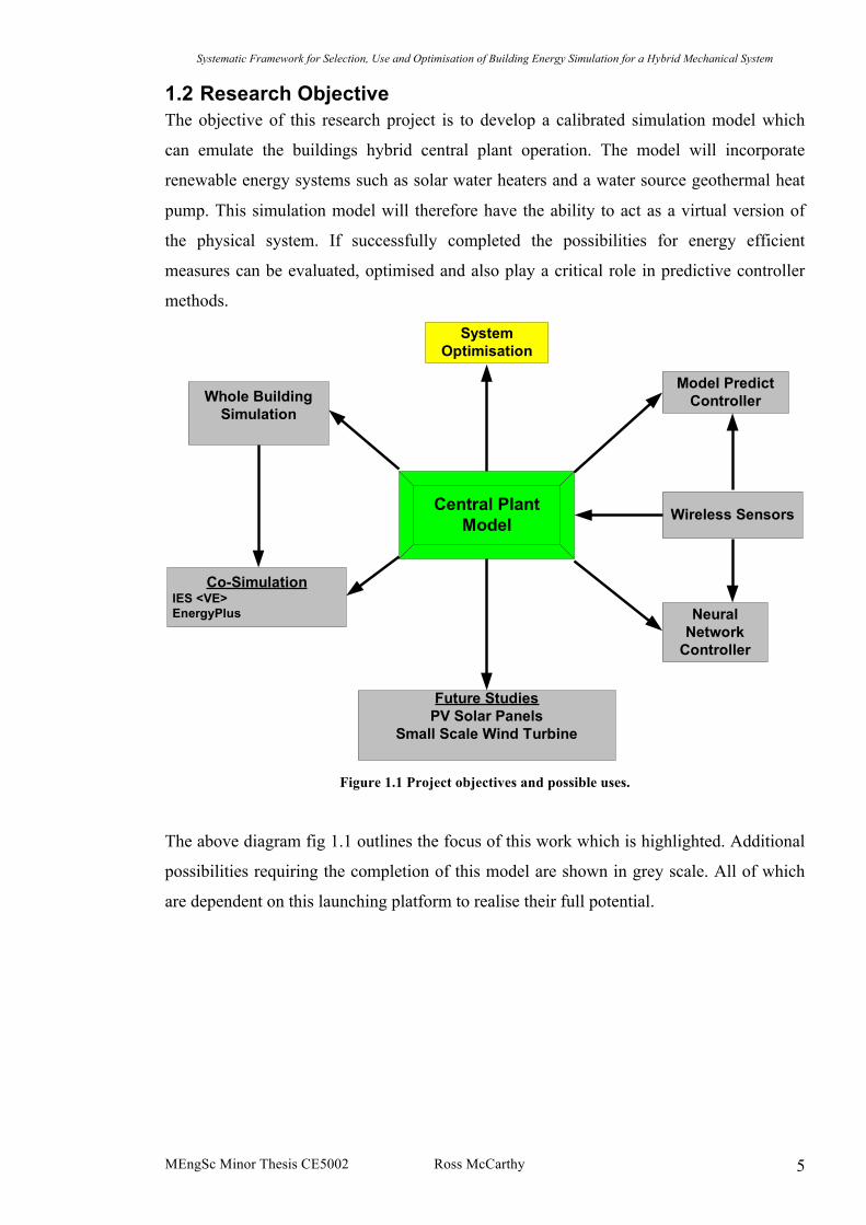
1.2 Research Objective The objective of this research project is to develop a calibrated simulation model which
can emulate the buildings hybrid central plant operation. The model will incorporate
renewable energy systems such as solar water heaters and a water source geothermal heat
pump. This simulation model will therefore have the ability to act as a virtual version of
the physical system. If successfully completed the possibilities for energy efficient
measures can be evaluated, optimised and also play a critical role in predictive controller
methods.
Central PlantModel
SystemOptimisation
Model PredictControllerWhole Building
Simulation
NeuralNetwork
Controller
Co-SimulationIES <VE>EnergyPlus
Future StudiesPV Solar Panels
Small Scale Wind Turbine
Wireless Sensors
Figure 1.1 Project objectives and possible uses.
The above diagram fig 1.1 outlines the focus of this work which is highlighted. Additional
possibilities requiring the completion of this model are shown in grey scale. All of which
are dependent on this launching platform to realise their full potential.
Systematic Framework for Selection, Use and Optimisation of Building Energy Simulation for a Hybrid Mechanical System
MEngSc Minor Thesis CE5002 Ross McCarthy 6
1.3 Project Scope This document can be summarised as follows;
Simulation Software Selection
• Required capabilities.
• Mathematical approaches.
• Initial selection of twenty leading programs.
• Detailed Review of most capable program.
• Selected simulation program.
Model Implementation
• Compiling the model and choosing components
• Controllers required
• Model inputs required from the BMS
Model Outputs
• Initial Outputs
• Adjustments made to model
• Final outputs
• Model Calibration and methodology
Model and Central Plant Optimisation methodology
• Parameters identified for energy saving
• A Proposed method
1.4 Buildings Current Energy Use The energy targets of this building were envisaged to be “very good” by the Building
Research establishment Environmental Assessment Method (BREEAM) rating. Outlined
as follows:
• Electrical energy demand of 60 kWh/m²/annum
• Natural Gas demand of 47 kWh/m²/annum
• Total energy demand of 107 kWh/m²/annum
The measured energy demands thus far are as follows (Swift L., 2007)
• Electrical energy demand of 71 kWh/m²/annum
• Natural Gas demand of 83 kWh/m²/annum
• Total energy demand of 154 kWh/m²/annum

Systematic Framework for Selection, Use and Optimisation of Building Energy Simulation for a Hybrid Mechanical System
MEngSc Minor Thesis CE5002 Ross McCarthy 7
2 Simulation Software Selection
The current available building energy simulation tools are investigated to ascertain their
ability to complete the task. The component based plant model will be applied in full scale
for all the subsystems of the central plant, together with the required control and operating
functions in order to emulate the operating characteristics of the mechanical equipment
within the plant-room.
2.1 Simulation Approach In the development of the central plant simulation model, just linking up all the related
components of equipment and pipework will not simulate the plants operation with
differing loads and climatic conditions throughout the simulated period. Additional
operation and control inputs will be necessary, so that the operating quantity and capacity
of the equipment, as well as the corresponding flow conditions at different portions of
pipework, can be effectively converged through the successive iteration processes (Fong
K.F., 2005). HOT WATER METER(OUTPUT)
SOLAR PANELSMETER (INPUT) AHU COIL METER
(OUTPUT)
BOILER HEAT METER(INPUT) +GAS
UNDERFLOOR HEATINGMETER (OUTPUT)
HEATPUMP METER(INPUT) + ELECTRICITY
WEATHER FILE (INPUT)
Figure 2.1 Model Inputs and Outputs (BMS screen shot)
The central plant model will only then truly reflect the physical system with complete
dynamic operation of the main mechanical plant and associated subsystems for the
fluctuating heating demand throughout the simulated period. The model will be driven by
historical BMS loads used as inputs to the model imposing loads on the simulated
mechanical plant.
Systematic Framework for Selection, Use and Optimisation of Building Energy Simulation for a Hybrid Mechanical System
MEngSc Minor Thesis CE5002 Ross McCarthy 8
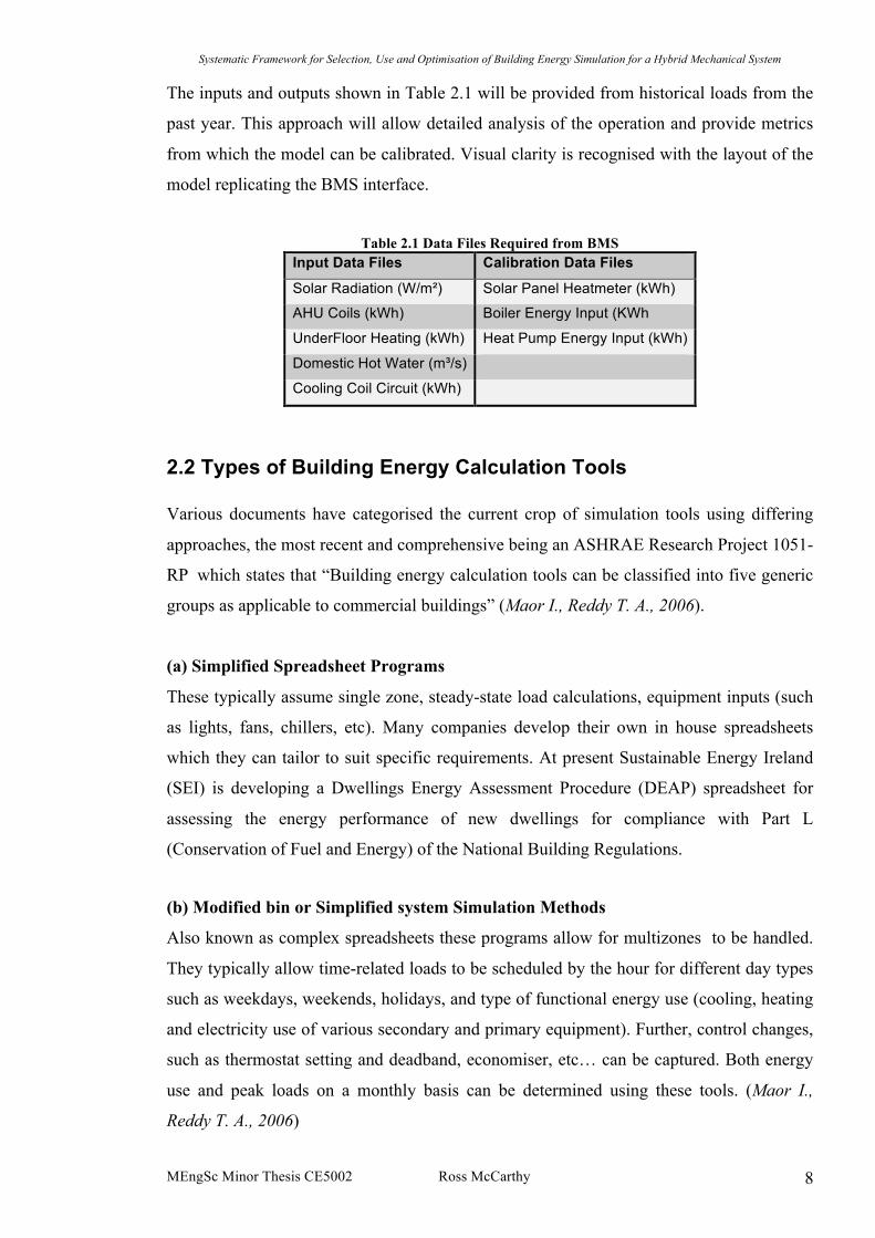
The inputs and outputs shown in Table 2.1 will be provided from historical loads from the
past year. This approach will allow detailed analysis of the operation and provide metrics
from which the model can be calibrated. Visual clarity is recognised with the layout of the
model replicating the BMS interface.
Table 2.1 Data Files Required from BMS
Input Data Files Calibration Data Files
Solar Radiation (W/m²) Solar Panel Heatmeter (kWh)
AHU Coils (kWh) Boiler Energy Input (KWh
UnderFloor Heating (kWh) Heat Pump Energy Input (kWh)
Domestic Hot Water (m³/s)
Cooling Coil Circuit (kWh)
2.2 Types of Building Energy Calculation Tools Various documents have categorised the current crop of simulation tools using differing
approaches, the most recent and comprehensive being an ASHRAE Research Project 1051-
RP which states that “Building energy calculation tools can be classified into five generic
groups as applicable to commercial buildings” (Maor I., Reddy T. A., 2006).
(a) Simplified Spreadsheet Programs
These typically assume single zone, steady-state load calculations, equipment inputs (such
as lights, fans, chillers, etc). Many companies develop their own in house spreadsheets
which they can tailor to suit specific requirements. At present Sustainable Energy Ireland
(SEI) is developing a Dwellings Energy Assessment Procedure (DEAP) spreadsheet for
assessing the energy performance of new dwellings for compliance with Part L
(Conservation of Fuel and Energy) of the National Building Regulations.
(b) Modified bin or Simplified system Simulation Methods
Also known as complex spreadsheets these programs allow for multizones to be handled.
They typically allow time-related loads to be scheduled by the hour for different day types
such as weekdays, weekends, holidays, and type of functional energy use (cooling, heating
and electricity use of various secondary and primary equipment). Further, control changes,
such as thermostat setting and deadband, economiser, etc… can be captured. Both energy
use and peak loads on a monthly basis can be determined using these tools. (Maor I.,
Reddy T. A., 2006)
Systematic Framework for Selection, Use and Optimisation of Building Energy Simulation for a Hybrid Mechanical System
MEngSc Minor Thesis CE5002 Ross McCarthy 9
(c) Fixed schematic hourly Simulation Programs
Such as Blast (BSL 1999) and DOE-2 which are commonly used general purpose
simulation tools. These programs are capable of simulating loads, systems, plant and
economics. Although the building loads-modelling module captures transient behaviour,
the algorithms for both secondary and primary systems are steady state (Maor I., Reddy T.
A., 2006).
(d) Modular Variable Time-step Simulation Programs
These programs include TRNSYS (Klein et al. 2004) and ESP-r (ESRU 2005, Clarke
2001) which are capable of determining complete transient and dynamic interaction of
buildings. All thermal based mechanical and fluid flow elements associated with comfort
and energy to be simulated under specified control action using built-in subroutines for
psychrometric and other fluid property determination (Maor I., Reddy T. A., 2006). Both of
these programs are discussed in more detail later in this chapter.
EnergyPlus (Crawley et al. 2004) is currently being developed as a modular variable time
step program based on the strongest attributes of both DOE-2 and BLAST. Previous efforts
to develop a whole building simulation model of UCC Environmental Research Institute
(Morrissey E., IRUSE 2006) have shown this program is limited in its current development
stage.
(e) Specialised Simulation Programs
Specialised programs have been developed through the years to solve specific tasks such as
moisture control, air movement, stratification, plant systems. Many use powerful
mathematical programs, such as Matlab/Simulink with tool boxes such as SimBad
(Riederer 2005).
Programs capable of emulating and assessing control strategies include the modular
variable time step-simulation programs previously mentioned but commercial tools such as
UniSim (Honeywell, 2007) offer a commercially available solution compared to high end
design or research tools.

Systematic Framework for Selection, Use and Optimisation of Building Energy Simulation for a Hybrid Mechanical System
MEngSc Minor Thesis CE5002 Ross McCarthy 10
2.2.1 Types of Inverse Models With recent focus and developments in renewable energy solutions for the built
environment, the need for more capable tools has become evident. This is particularly true
for retro-fit and post construction optimisation where commercial design tools have been
found to be imprecise and inadequate. The subsequent interest in this area has led to the
development of more specialised inverse (or data driven) modelling and analysis methods which
use monitored energy data from the building along with other variables such as climatic variables
(Maor I., Reddy T. A., 2006).
Though a consensus is still lacking in the building professional community, inverse
methods for energy use estimation in buildings and related equipment can be classified into
three broad approaches (Reddy T.A., Anderson, 2002). These approaches are described
briefly as follows:
(a) Black-Box Model
Energy data/metrics obtained from building along with weather dependent and weather
independent loads (internal loads/gains, occupancy, external climate, etc) can be used to
create simple or multi-variable statistical model. A program such as Matlab can also be
used to formulate basic engineering equations or purely database driven models to describe
an operation. The physical meaning of this approach in terms of emulating a system is
crude and restricted for purposes of retro-fit analysis and post-construction optimisation.
(b) Grey-box or Parameter Estimation Model
This approach is similar to a black box model, however more detailed mechanistic models
are used for the HVAC equipment which allows are greater flexibility. Again a program
such a Matlab/Simulink is an example with various toolboxes available at commercial and
research levels.
(c) Calibrated Simulation
This approach uses an existing building simulation program and “tunes” or calibrates the
various physical inputs to the program so that observed energy use matches closely with
that predicted by the simulation program (Stein, 1997). This approach can salvage pre-
construction design simulation and apply them for optimisation/retro-fit analysis.
Calibration techniques are discussed in more detail in Chapter 4. Furthermore, simulation
programs which lack the required capabilities can be coupled with programs such as
TRNSYS, this approach is discussed in chapter 5 which outlines methods for co-simulation

Systematic Framework for Selection, Use and Optimisation of Building Energy Simulation for a Hybrid Mechanical System
MEngSc Minor Thesis CE5002 Ross McCarthy 11
using either an IES or EnergyPlus models of the Environmental Research Institute. This
approach provides a platform for more reliable and insightful prediction compared with
statistical models.
2.3 Review of Building Energy Software Tools In this section, an assessment of the current capabilities of building energy performance
simulation programs applied to modelling the central plant of the ERI building is
conducted. The Building Energy Software Tools Directory lists over 290 programmes for
buildings energy efficiency evaluation (DOE, 2005). A comparison of the features and
capabilities of twenty leading programs is shown below in Table 2.3. The list includes
both fixed schematic hourly simulation programs and modular variable time-step
simulation programs. Table 2.3 Leading Building Energy Simulation Programs
Ener-Win eQUEST IES<VE>
Energy Express ESP-r HAP
Energy-10 IDA ICE HEED
EnergyPlus TRNSYS SUNREL
PowerDomuus TAS TRACE
BLAST BSim DeST
ECOTECT DOE-2.1E
The Comparison study has been published by (Kummert et al. 2005) and has been
modified to provide an initial selection of these programs to be compared in more detail
and to include MatLab/Simulink. A total of 7 tables (Appendix B) have been used to
evaluate the above programs in each of the following areas: General Modelling Features,
Zone Loads, Renewable Energy Systems, Electrical Systems and Equipment and HVAC
Systems.
Systematic Framework for Selection, Use and Optimisation of Building Energy Simulation for a Hybrid Mechanical System
MEngSc Minor Thesis CE5002 Ross McCarthy 12
2.4 Mechanical Systems Modelling Requirements It is important to note that this method was used to select initial programs which would
later require further investigation. Partially implemented features were not included in this
assessment. The assessed tables (Appendix B) are based on vendor-supplied information
and were generated by collaboration of experts and published in 2005. It represents the
most recent and comprehensive study of building energy simulation tools. Appendix A
Reference: Crawley D, Hand J, Kummert M, Griffth B, 2005 “Contrasting the Capabilities
of Building Energy Performance Simulation Programs”.
2.4.1 General Modelling features This table provides an overview of how the various tools approach the solution of the
buildings and systems described in a programmers model, the frequency of the solution,
the geometric elements which zones can be composed and exchange supported with other
CAD and simulation tools. The table indicates that the majority of tools support the
simultaneous solution of building and environmental systems. A few tools support
exchange data with other simulation tools so that second numerical opinions can be
acquired without having to re-enter all model details.
2.4.2. Zone loads This table provides an overview of tool support for solving the thermophysical state of
rooms: whether there is a heat balance underlying the calculations, how conduction and
convection within rooms are solved, and the extent to which thermal comfort can be
assessed. The majority of vendors claim a heat balance approach although few of these
report energy balance (see Table 12). This table indicates considerable variation in
facilities on offer. Eight tools claim no support for thermal comfort. Of those that do,
Fanger's PMV and PPD indices and mean radiant temperature are used by a majority of
tools that calculate comfort. The table indicates that there is a sub-set of tools supporting
additional inside surface convection options. Most tools claim support for internal thermal
mass, but the specifics are not yet included in the table. Users would need to check the
vendors’ web sites for further detail.

Systematic Framework for Selection, Use and Optimisation of Building Energy Simulation for a Hybrid Mechanical System
MEngSc Minor Thesis CE5002 Ross McCarthy 13
2.4.3. Renewable Energy Systems ability This brief table provides an overview of renewable energy systems. The table is based on
entries suggested by vendors and is not yet complete in terms of its coverage of such
designs, what is required of the programmer is to define such designs or the performance
indicators that are reported. With a few exceptions, vendors have few facilities for such
assessments.
2.4.4. Electrical Systems and Equipment This table provides an overview of how electrical systems and equipment are treated in
each tool. The majority of tools claim support for building power loads. Yet most of these
loads are simply scheduled inputs. As with renewable energy systems, support for
electrical engineers is sparse.
2.4.5. HVAC Systems modelling capabilities This table provides an overview of HVAC systems, with additional sections for demand-
controlled ventilation, CO2 control and sizing. Readers should also consult Table 8, which
has sections for other environmental control systems and components. At the beginning of
the table is an indicator as to whether HVAC systems are composed from discrete
components (implying that the programmer has some freedom in the design of the system)
or that there are system templates provided. It is notable that some tools now claim to
support CO2 sensor control of HVAC systems. Automatic sizing is offered by quite a few
tools. Most tools offer a range of zonal and room air distribution devices.
2.4.6. Available HVAC equipment components This table provides an overview of the HVAC components as well as components used in
central plant modelling as well as components associated with domestic hot water. This
table is diverse because it reflects the diversity that vendors currently support. Such
diversity requires the programmer to scan the full table for items of interest.

Systematic Framework for Selection, Use and Optimisation of Building Energy Simulation for a Hybrid Mechanical System
MEngSc Minor Thesis CE5002 Ross McCarthy 14
2.5 Initial Software Selection In the initial software selection no distinction has been made between single simulation
tools or modular programs utilising a suite of tools, however a modular approach is
preferable as it will allow the specific simulation needs to be adopted. It was determined
that both ESP-r and TRNSYS were equally matched whilst EnergyPlus and IDA-ICE also
favoured highly and therefore warrant further analyses. In the next section, each will be
discussed in more detail along with MatLab/Simulink.
2.6 ESP- rESP-r (ESRU 2005, Clarke 2001) version 10.1 is a general purpose, multi-domain-building
thermal, interzone airflow, intra-zone air movement, HVAC systems and electrical flow-
simulation environment which has been under development for more than 25years.
It follows the pattern of ‘simulation follows description’ where additional technical domain
solvers are invoked as the building and system description evolves. Programmers control
the complexity of the geometric, environmental control and operations to match the
requirements of particular projects. Recent examples include Navan town Credit Union
building which required a tool capabilities for modelling complex systems.
Figure 2.6.1 ESP-r screenshot showing interface

Systematic Framework for Selection, Use and Optimisation of Building Energy Simulation for a Hybrid Mechanical System
MEngSc Minor Thesis CE5002 Ross McCarthy 15
2.6.1 Modelling Approach It uses a simultaneous modular integration approach (Trcka et al 2006). System parts are
represented by deriving a set of time averaged heat and mass balance equations. The
system matrix is then solved for each time step obtaining the simultaneous solution for the
overall system. However, the mass balance matrix equations are solved sequentially,
applying iterations if the difference between assumed and final values of the marked
variables exceeds specified tolerance (Hensen et al 2006).
It works with third party tools such as Radiance to support higher resolution assessments as
well as interacting with supply and demand matching tools (Crawley et al 2005). An
extensive publications list exists along with example models, cross-referenced source code,
tutorials. It can also run on any platform and operating system.
2.6.2 Controls System control is explicitly modelled, defining;
o Sensor location and sensed variable,
o Actuator location and actuated variable
o Control low with its settings
Control variable(s) for each component is predetermined by the model algorithm itself. It
does not always have a real world complement. Different sensor/actuator/control low
combinations are possible. There are various (although limited number of) controllers in
the software database.
Systematic Framework for Selection, Use and Optimisation of Building Energy Simulation for a Hybrid Mechanical System
MEngSc Minor Thesis CE5002 Ross McCarthy 16
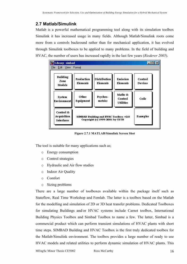
2.7 Matlab/Simulink Matlab is a powerful mathematical programming tool along with its simulation toolbox
Simulink it has increased usage in many fields. Although Matlab/Simulink roots come
more from a controls backround rather than for mechanical application, it has evolved
through Simulink toolboxes to be applied to many problems. In the field of building and
HVAC, the number of users has increased rapidly in the last few years (Riederer 2005).
Figure 2.7.1 MATLAB/Simulink Screen Shot
The tool is suitable for many applications such as;
o Energy consumption
o Control strategies
o Hydraulic and Air flow studies
o Indoor Air Quality
o Comfort
o Sizing problems
There are a large number of toolboxes available within the package itself such as
Stateflow, Real Time Workshop and Femlab. The latter is a toolbox based on the Matlab
for the modelling and simulation of 2D or 3D heat transfer problems. Dedicated Toolboxes
for simulating Buildings and/or HVAC systems include Carnot toolbox, International
Building Physics Toolbox and Simbad Toolbox to name a few. The latter, Simbad is a
commercial product which can perform transient simulations of HVAC plants with short
time steps. SIMBAD Building and HVAC Toolbox is the first truly dedicated toolbox for
the Matlab/Simulink environment. The toolbox provides a large number of ready to use
HVAC models and related utilities to perform dynamic simulation of HVAC plants. This
Systematic Framework for Selection, Use and Optimisation of Building Energy Simulation for a Hybrid Mechanical System
MEngSc Minor Thesis CE5002 Ross McCarthy 17
toolbox, in connection with other existing toolboxes (neural network, fuzzy logic, and
optimisation) offers a powerful and efficient tool for design and test of controllers.
By combining several toolboxes it is possible to model most systems. The large number of
available toolboxes does not come without problems. Most notable is the fragmented
nature of inputs and outputs defined by different developers and their subsequent
interoperability. Currently there is no convention to define the start and finish of modules
to allow ease of integration.
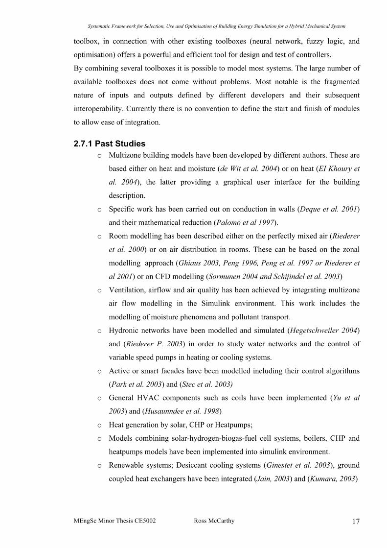
2.7.1 Past Studies o Multizone building models have been developed by different authors. These are
based either on heat and moisture (de Wit et al. 2004) or on heat (EI Khoury et
al. 2004), the latter providing a graphical user interface for the building
description.
o Specific work has been carried out on conduction in walls (Deque et al. 2001)
and their mathematical reduction (Palomo et al 1997).
o Room modelling has been described either on the perfectly mixed air (Riederer
et al. 2000) or on air distribution in rooms. These can be based on the zonal
modelling approach (Ghiaus 2003, Peng 1996, Peng et al. 1997 or Riederer et
al 2001) or on CFD modelling (Sormunen 2004 and Schijindel et al. 2003)
o Ventilation, airflow and air quality has been achieved by integrating multizone
air flow modelling in the Simulink environment. This work includes the
modelling of moisture phenomena and pollutant transport.
o Hydronic networks have been modelled and simulated (Hegetschweiler 2004)
and (Riederer P. 2003) in order to study water networks and the control of
variable speed pumps in heating or cooling systems.
o Active or smart facades have been modelled including their control algorithms
(Park et al. 2003) and (Stec et al. 2003)
o General HVAC components such as coils have been implemented (Yu et al
2003) and (Husaunndee et al. 1998)
o Heat generation by solar, CHP or Heatpumps;
o Models combining solar-hydrogen-biogas-fuel cell systems, boilers, CHP and
heatpumps models have been implemented into simulink environment.
o Renewable systems; Desiccant cooling systems (Ginestet et al. 2003), ground
coupled heat exchangers have been integrated (Jain, 2003) and (Kumara, 2003)

Systematic Framework for Selection, Use and Optimisation of Building Energy Simulation for a Hybrid Mechanical System
MEngSc Minor Thesis CE5002 Ross McCarthy 18
The fact that Matlab/Simulink is a multidiscipline tool owes itself to its success. The
relative ease of coupling modules from various fields means that it will continue to grow.
Its ability to import or export with other software will ensure its growth and will likely be
an important feature in newly developed or existing simulation software.
Systematic Framework for Selection, Use and Optimisation of Building Energy Simulation for a Hybrid Mechanical System
MEngSc Minor Thesis CE5002 Ross McCarthy 19
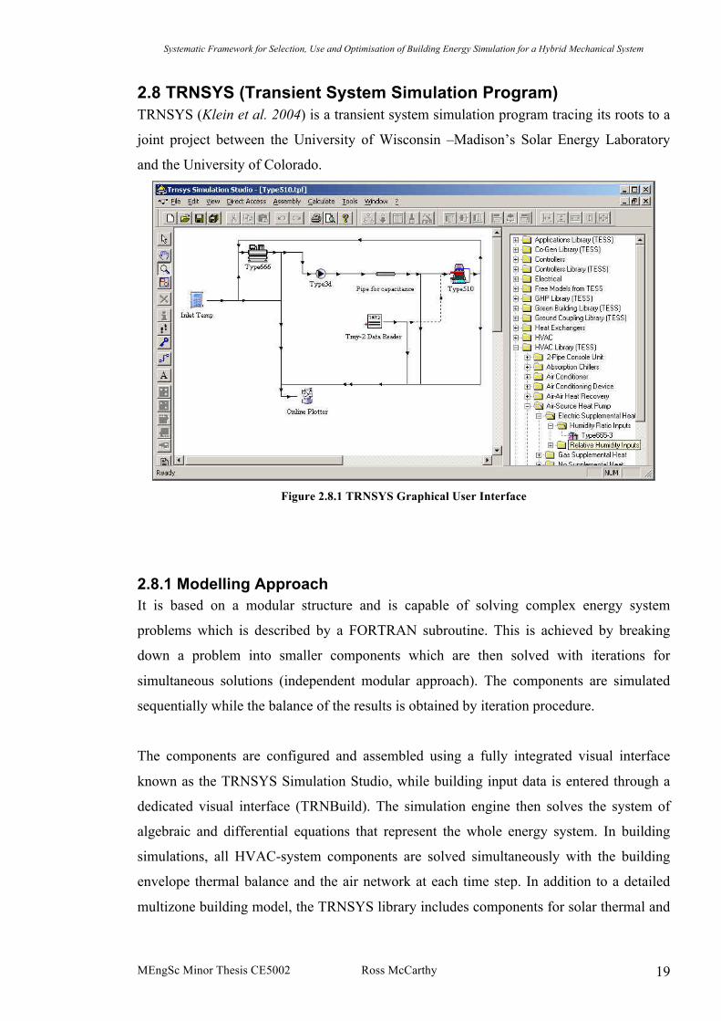
2.8 TRNSYS (Transient System Simulation Program) TRNSYS (Klein et al. 2004) is a transient system simulation program tracing its roots to a
joint project between the University of Wisconsin –Madison’s Solar Energy Laboratory
and the University of Colorado.
Figure 2.8.1 TRNSYS Graphical User Interface
2.8.1 Modelling Approach It is based on a modular structure and is capable of solving complex energy system
problems which is described by a FORTRAN subroutine. This is achieved by breaking
down a problem into smaller components which are then solved with iterations for
simultaneous solutions (independent modular approach). The components are simulated
sequentially while the balance of the results is obtained by iteration procedure.
The components are configured and assembled using a fully integrated visual interface
known as the TRNSYS Simulation Studio, while building input data is entered through a
dedicated visual interface (TRNBuild). The simulation engine then solves the system of
algebraic and differential equations that represent the whole energy system. In building
simulations, all HVAC-system components are solved simultaneously with the building
envelope thermal balance and the air network at each time step. In addition to a detailed
multizone building model, the TRNSYS library includes components for solar thermal and
Systematic Framework for Selection, Use and Optimisation of Building Energy Simulation for a Hybrid Mechanical System
MEngSc Minor Thesis CE5002 Ross McCarthy 20
photovoltaic systems, low energy buildings and HVAC systems, renewable energy
systems, cogeneration, fuel cells, etc.
The modular nature of TRNSYS facilitates the addition of new mathematical models to the
program. New components can be developed in any programming language and modules
implemented using other software (e.g. Matlab/Simulink, Excel/VBA, and EES) can also
be directly embedded in a simulation. TRNSYS can generate redistributable applications
that allow non-expert users to run simulations and parametric studies.
2.8.2 Controls The controls applicable to each problem are handled in an explicit manner, as in ESP-r.
However a greater number of controllers are available in its database.
System control is explicitly modelled, defining;
o Sensor location and sensed variable,
o Actuator location and actuated variable
o Control low with its settings
Control variable(s) for each component is predetermined by the model algorithm itself. It
does not always have a real world complement. Different sensor/actuator/control low
combinations are possible. There are various (although limited number of) controllers in
the software database.

Systematic Framework for Selection, Use and Optimisation of Building Energy Simulation for a Hybrid Mechanical System
MEngSc Minor Thesis CE5002 Ross McCarthy 21
2.9 EnergyPlus EnergyPlus (Crawley et al. 2004) was used in a previous attempt to generate a whole
building model of the ERI and failed primarily due to lack of flexibility in the mass energy
balance approach employed, it’s dedicated mechanical capabilities warrants a second look
though. The initial review of this program suggests a relatively strong capability from
vendor supplied information.
Figure 2.9.1 EnergyPlus Data Entry Interface Screen Shot
2.9.1 Modelling Approach It has an independent modular integration approach modular approach (Trcka et al 2006).
EnergyPlus system representation is based on fluid loops, all system components are
attached to them. Most of the components are modelled in steady state fashion.
The loops define the movement of mass and energy within the system and a difference is
made between the air loop, plant loop and condenser loop. The loops are indirectly
connected and each has two logical simulation blocks, supply and demand side. The
demand side places a load to the supply side are both are simulated independently, while
the convergence between their interaction points is checked and if necessary the iteration is
required to ensure that the results among the loops are balanced.
Systematic Framework for Selection, Use and Optimisation of Building Energy Simulation for a Hybrid Mechanical System
MEngSc Minor Thesis CE5002 Ross McCarthy 22
2.9.2 Controls The control modelling is less explicit than that of ESP-r, TRNSYS or MatLab/Simulink.
The representation of control is somewhat artificial, since it uses the knowledge of the
zone load (ERI model required systems to span more than one zone) which is only
available in the simulation model, but not in reality (EnergyPlus 2005). The control is
modelled using a two level system of controllers and set point managers. The controller
can not span a loop manager boundary, meaning that the sensed node and the controlled
device must be in the same loop. The set point manager is able to cross the loop manager
boundary, but this does not represent the building accurately, especially mixed use
buildings.
The user specified time step is currently limited to 10 minutes to ensure the stability of the
results, an adaptive time step that is calculated during run-time, is used for system
simulation and zone temperature updates.
See Appendix C.
Systematic Framework for Selection, Use and Optimisation of Building Energy Simulation for a Hybrid Mechanical System
MEngSc Minor Thesis CE5002 Ross McCarthy 23
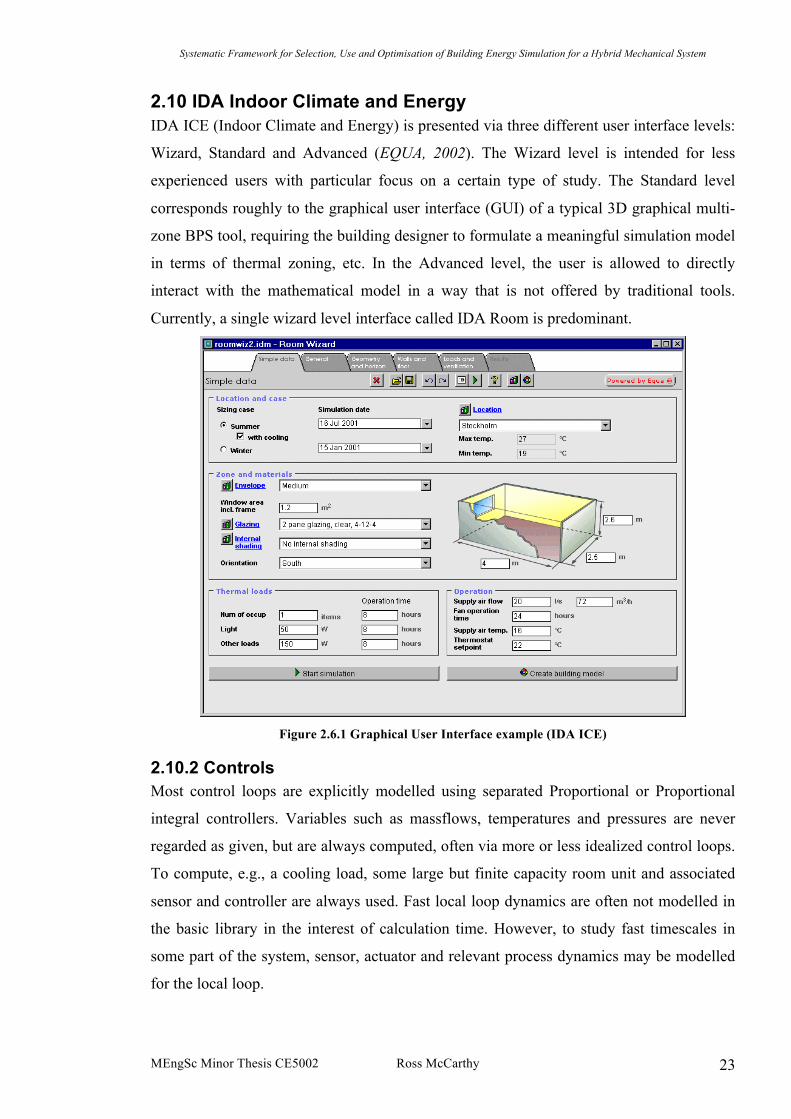
2.10 IDA Indoor Climate and Energy IDA ICE (Indoor Climate and Energy) is presented via three different user interface levels:
Wizard, Standard and Advanced (EQUA, 2002). The Wizard level is intended for less
experienced users with particular focus on a certain type of study. The Standard level
corresponds roughly to the graphical user interface (GUI) of a typical 3D graphical multi-
zone BPS tool, requiring the building designer to formulate a meaningful simulation model
in terms of thermal zoning, etc. In the Advanced level, the user is allowed to directly
interact with the mathematical model in a way that is not offered by traditional tools.
Currently, a single wizard level interface called IDA Room is predominant.
Figure 2.6.1 Graphical User Interface example (IDA ICE)
2.10.2 Controls Most control loops are explicitly modelled using separated Proportional or Proportional
integral controllers. Variables such as massflows, temperatures and pressures are never
regarded as given, but are always computed, often via more or less idealized control loops.
To compute, e.g., a cooling load, some large but finite capacity room unit and associated
sensor and controller are always used. Fast local loop dynamics are often not modelled in
the basic library in the interest of calculation time. However, to study fast timescales in
some part of the system, sensor, actuator and relevant process dynamics may be modelled
for the local loop.
Systematic Framework for Selection, Use and Optimisation of Building Energy Simulation for a Hybrid Mechanical System
MEngSc Minor Thesis CE5002 Ross McCarthy 24
2.11 Selected Software From examining the above simulation software, it is evident that either TRNSYS or ESP-r
would be compared to MATLAB/Simulink (including SIMBAD toolbox). A lack of
published papers concerning ICA ICE compared to the others discouraged its use in this
problem. MATLAB or indeed SIMBAD fares better but again compared to TRNSYS and
ESP-r is relatively new. A demo of SIMBAD could not be downloaded to evaluate ease of
use. Both ESP-r and TRNSYS were downloaded. ESP-r was difficult to get started with
and upon reading its manuals, self learning was difficult plus the observation that most
papers concerning complex problems were done within Strathclyde University itself.
Finally, TRNSYS was chosen for better GUI (graphical user interface), larger user
numbers, and a large library of controls and general ease of use. The programmer can be
confident with technical support from TESS (Thermal Energy Systems Specialists) and a
large development group worldwide.
TRNSYS is one of the listed simulation programs in the recent European standards on
solar thermal systems (ENV-12977-2). The level of detail of TRNSYS ’building model,
known as ‘‘Type 56’’, is compliant with the requirements of ANSI/ASHRAE Standard
140–2001.
The level of detail of Type 56 also meets the general technical requirements of the
European directive on the energy performance of buildings (NN, Directive
2002/91/EC.2002.)
Systematic Framework for Selection, Use and Optimisation of Building Energy Simulation for a Hybrid Mechanical System
MEngSc Minor Thesis CE5002 Ross McCarthy 25
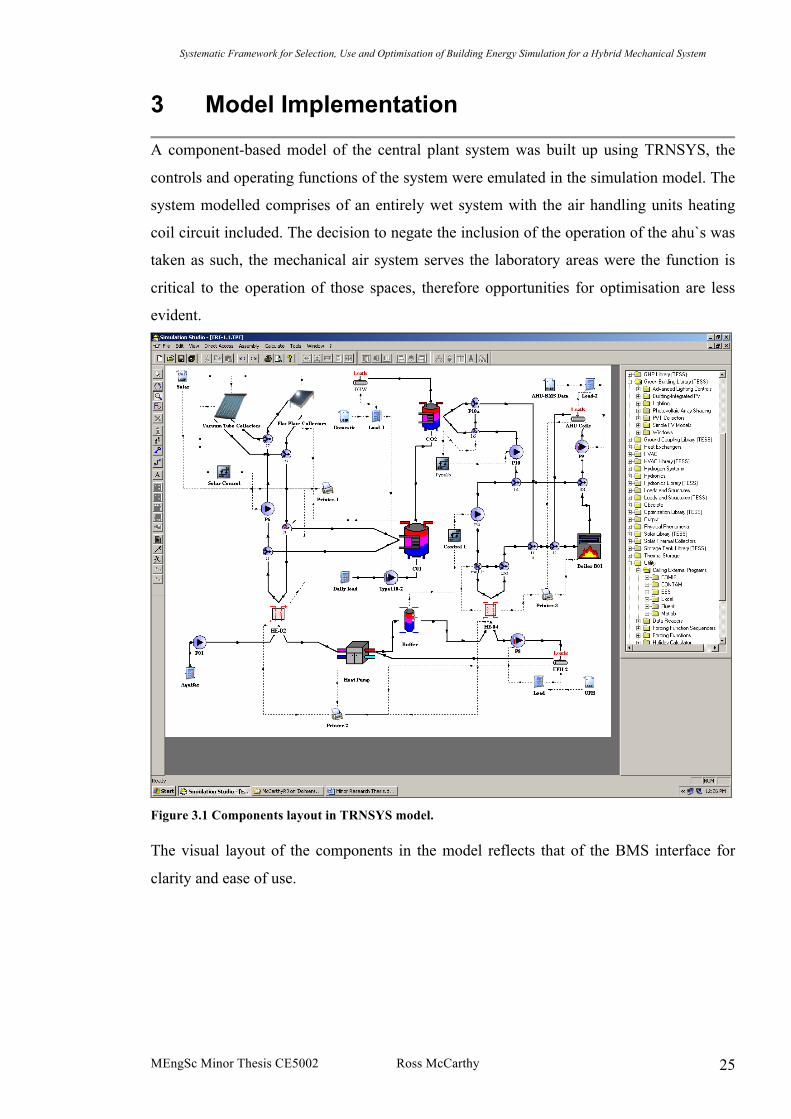
3 Model Implementation
A component-based model of the central plant system was built up using TRNSYS, the
controls and operating functions of the system were emulated in the simulation model. The
system modelled comprises of an entirely wet system with the air handling units heating
coil circuit included. The decision to negate the inclusion of the operation of the ahu`s was
taken as such, the mechanical air system serves the laboratory areas were the function is
critical to the operation of those spaces, therefore opportunities for optimisation are less
evident.
Figure 3.1 Components layout in TRNSYS model. The visual layout of the components in the model reflects that of the BMS interface for
clarity and ease of use.

Systematic Framework for Selection, Use and Optimisation of Building Energy Simulation for a Hybrid Mechanical System
MEngSc Minor Thesis CE5002 Ross McCarthy 26
3.1 Main Components Multiple choices are available when choosing components or types within TRNSYS. The
selection of which is determined by factors such as available data both measured and
vendor supplied, complexity and calibration parameters. The latter of which will be
required to rectify inaccuracies between real and simulated results.
A time step of 30 seconds was chosen as it represents 10% of the dominant step. The
dominant time step is 300 sec, which is the sampling rate of data from the BMS. This will
ensure stability in the model.
3.1.1 Flat Plate Solar Panels This component (Type 1) models the thermal performance of the flat plate collectors using
theory along with Viessmann product information. The collector array consists of 24
panels connected in series. The vacuum tubes are also connected in series with this array.
The model assumes that the efficiency vs. ΔT/l T curve can be modelled as a quadratic
equation. Corrections are applied to the slope, intercept, and curvature parameters to
account for the presence of a heat exchanger, identical collectors in series, and flow rates
other than those at test conditions (Klein et al., 2004, TRNSYS 16).
The effects of off-normal solar incidence are not considered in this model. Table 3.1.1
shows the required parameters and inputs used for this component. A Data Reader for
Generic Data Files (Type 9) was used to input direct solar radiance. Table 3.1.1 Flat plate solar panels data.
Parameters Inputs
Number in series 24 Inlet Temperature 20°C
Collector area 2.5m² Inlet Flowrate 0.05kg/s
Fluid Specific heat capacity 4.19kJ/kg.K Ambient temperature 10°C
Collector fin efficiency factor 0.7 Incident Radiation Type-9
Bottom, edge loss coefficient 0.8W/m².k Ground reflectance 0.2
Absorber plate emittance 0.7 Incident angle 35
Aborptance of absorber plate 0.8
Number of covers 1
Index of refraction of cover 1.526

Systematic Framework for Selection, Use and Optimisation of Building Energy Simulation for a Hybrid Mechanical System
MEngSc Minor Thesis CE5002 Ross McCarthy 27
3.1.2 Evacuated Tube Solar Collectors The thermal efficiency of this component (Type71) is identical to the flat panel solar
panels. The component is modelled using a quadratic efficiency curve and a biaxial
Incidence Angle Modifiers.
Table 3.1.2 Evacuated Tube Solar Collector Data
Parameters Inputs
Number in series 24 Inlet Temperature 20°C
Collector area 2.0m² Inlet Flowrate 0.08kg/s
Fluid Specific heat capacity 4.19kJ/kg.K Ambient temperature
10°C
Collector efficiency mode 1.0 Incident Radiation Ext.
Flowrate at test conditions 3kg/s.m² Ground reflectance
0.2
Intercept efficiency mode 0.7 Incident angle 35
Negative of first order Efficiency coefficient
10 kJ/hr.m².K
Negative of second order Efficiency coefficient
0.03 kJ/hr.m².K
Index of refraction of cover 1.526
3.1.3 Pumps General Constant Speed:
This component models the constant speed pumps that are able to maintain a constant fluid
outlet mass flowrate. The starting and stopping characteristics are not modelled in this type
(Type114). Therefore, as soon as the control signal indicates that the pump should be ON,
the outlet flow of fluid will jump to its rated condition. This is due to the time constants
with which pumps react in the model to control signal changes is shorter than the input
time step from the data reader ie. 30 sec simulation time step versus 300sec BMS data.
Table 3.1.2 Pump Components Data
Parameters Inputs
Rated flow rates Kg/s Inlet Temperature °C
Fluid Specific heat capacity 4.19kJ/kg.K Inlet Flow rate kg/s
Rated Power kW Control signal 0-1
Motor heat loss fraction 0 Overall pump efficiency 0.6
Flowrate at test conditions 3kg/s.m² Motor efficiency 0.9
Variable Speed:
This component (Type 110) models the variable speed pumps in the system and is able to
maintain any mass outlet flow rate between zero and rated value. The mass flow rate of the

Systematic Framework for Selection, Use and Optimisation of Building Energy Simulation for a Hybrid Mechanical System
MEngSc Minor Thesis CE5002 Ross McCarthy 28
pump varies linearly with control signal setting. The control signal is determined using an
Equation editor; values between 0 and 1 are calculated as a function of the maximum
flowrate.
As with the constant speed component starting and stopping characteristics are not
considered and the outlet flow of fluid jumps to the appropriate value between 0 and its
rated (MAX) condition 1.
3.1.4 Plate Heat Exchangers This component (Type 5) is modelled as a zero capacitance sensible heat exchanger and is
configured for counter flow mode. The hot and cold side inlet temperatures and flow rates
are inputs. The effectiveness is calculated for a given fixed value of the overall heat
transfer coefficient.
This component relies on an effectiveness minimum capacitance approach to modelling a
heat exchanger. Under this assumption, the inlet conditions are provided. The model then
determines whether the cold or hot side is the minimum (load and source sides)
capacitance side and calculates effectiveness based upon the specified flow configuration
(Klein et al., 2004, TRNSYS 16). The outputs are then computed.
Table 3.1.4 Plate Heat Exchanger Data
Parameters Inputs
Counter flow mode 2 Hot side inlet temperature °C
Specific heat of hot side fluid
4.19kJ/kg.K Hot side flow rate kg/s
Specific heat of cold side fluid
4.19kJ/kg.K Cold side inlet temperature °C
Cold side flow rate kg/s
Overall heat transfer coeff. of exchanger
0.9
Systematic Framework for Selection, Use and Optimisation of Building Energy Simulation for a Hybrid Mechanical System
MEngSc Minor Thesis CE5002 Ross McCarthy 29
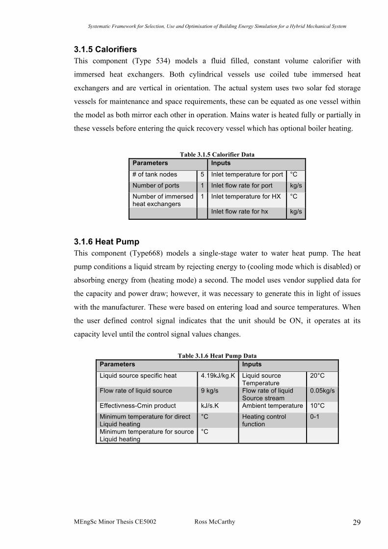
3.1.5 Calorifiers This component (Type 534) models a fluid filled, constant volume calorifier with
immersed heat exchangers. Both cylindrical vessels use coiled tube immersed heat
exchangers and are vertical in orientation. The actual system uses two solar fed storage
vessels for maintenance and space requirements, these can be equated as one vessel within
the model as both mirror each other in operation. Mains water is heated fully or partially in
these vessels before entering the quick recovery vessel which has optional boiler heating.
Table 3.1.5 Calorifier Data
Parameters Inputs
# of tank nodes 5 Inlet temperature for port °C
Number of ports 1 Inlet flow rate for port kg/s
Number of immersed heat exchangers
1 Inlet temperature for HX °C
Inlet flow rate for hx kg/s
3.1.6 Heat Pump This component (Type668) models a single-stage water to water heat pump. The heat
pump conditions a liquid stream by rejecting energy to (cooling mode which is disabled) or
absorbing energy from (heating mode) a second. The model uses vendor supplied data for
the capacity and power draw; however, it was necessary to generate this in light of issues
with the manufacturer. These were based on entering load and source temperatures. When
the user defined control signal indicates that the unit should be ON, it operates at its
capacity level until the control signal values changes.
Table 3.1.6 Heat Pump Data
Parameters Inputs
Liquid source specific heat 4.19kJ/kg.K Liquid source Temperature
20°C
Flow rate of liquid source 9 kg/s Flow rate of liquid Source stream
0.05kg/s
Effectivness-Cmin product kJ/s.K Ambient temperature 10°C
Minimum temperature for direct Liquid heating
°C Heating control function
0-1
Minimum temperature for source Liquid heating
°C
Systematic Framework for Selection, Use and Optimisation of Building Energy Simulation for a Hybrid Mechanical System
MEngSc Minor Thesis CE5002 Ross McCarthy 30
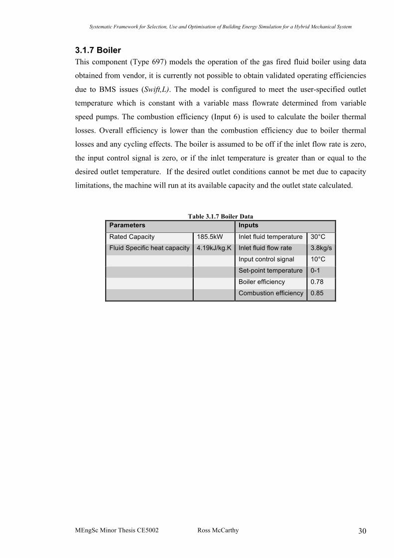
3.1.7 Boiler This component (Type 697) models the operation of the gas fired fluid boiler using data
obtained from vendor, it is currently not possible to obtain validated operating efficiencies
due to BMS issues (Swift,L). The model is configured to meet the user-specified outlet
temperature which is constant with a variable mass flowrate determined from variable
speed pumps. The combustion efficiency (Input 6) is used to calculate the boiler thermal
losses. Overall efficiency is lower than the combustion efficiency due to boiler thermal
losses and any cycling effects. The boiler is assumed to be off if the inlet flow rate is zero,
the input control signal is zero, or if the inlet temperature is greater than or equal to the
desired outlet temperature. If the desired outlet conditions cannot be met due to capacity
limitations, the machine will run at its available capacity and the outlet state calculated.
Table 3.1.7 Boiler Data Parameters Inputs
Rated Capacity 185.5kW Inlet fluid temperature 30°C
Fluid Specific heat capacity 4.19kJ/kg.K Inlet fluid flow rate 3.8kg/s
Input control signal 10°C
Set-point temperature 0-1
Boiler efficiency 0.78
Combustion efficiency 0.85
Systematic Framework for Selection, Use and Optimisation of Building Energy Simulation for a Hybrid Mechanical System
MEngSc Minor Thesis CE5002 Ross McCarthy 31
3.2 Dynamic Control and Operation The implementation of the central plant simulation model involves linking the main
components such as heat exchangers, pumps, boiler etc, however to reflect the real plant
operation under varying loads and climatic conditions further inputs were necessary. The
model therefore required operation and control inputs, so that the operating quantity and
capacity of the equipment, as well as the corresponding flow conditions at different
portions of pipework could be effectively converged through the successive iteration
processes.
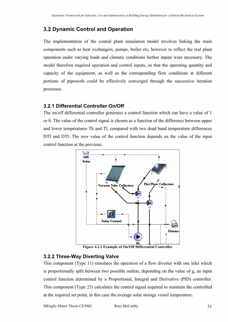
3.2.1 Differential Controller On/Off The on/off differential controller generates a control function which can have a value of 1
or 0. The value of the control signal is chosen as a function of the difference between upper
and lower temperatures Th and Tl, compared with two dead band temperature differences
DTI and DTI. The new value of the control function depends on the value of the input
control function at the previous.
Figure 4.2.1 Example of On/Off Differential Controller
3.2.2 Three-Way Diverting Valve This component (Type 11) simulates the operation of a flow diverter with one inlet which
is proportionally split between two possible outlets, depending on the value of g, an input
control function determined by a Proportional, Integral and Derivative (PID) controller.
This component (Type 23) calculates the control signal required to maintain the controlled
at the required set point, in this case the average solar storage vessel temperature.
Systematic Framework for Selection, Use and Optimisation of Building Energy Simulation for a Hybrid Mechanical System
MEngSc Minor Thesis CE5002 Ross McCarthy 32
3.3 Building Geometry This section briefly describes the building, although this research focuses on the central
plant an understanding of the subject will help in understanding the results of this study.
The buildings current energy performance metrics have been researched by Swift L., “Post
occupancy performance evaluation of the ERI using standardised building metrics” 2007.
3.3.1 Building Layout The building is rectangular in shape and consists of 3 floors on a sloped site with a partial
basement incorporated on the ground floor. The south façade utilises a high percentage
area fenestration with minimal shading provided from concrete columns.
The building provides several functions housing open plan and single offices, laboratories
and clean rooms. The layout is repeated over the first and second floor in three zones. The
ground floor differs with laboratories south facing and shading from above also and cold
stores and utilities to the rear.
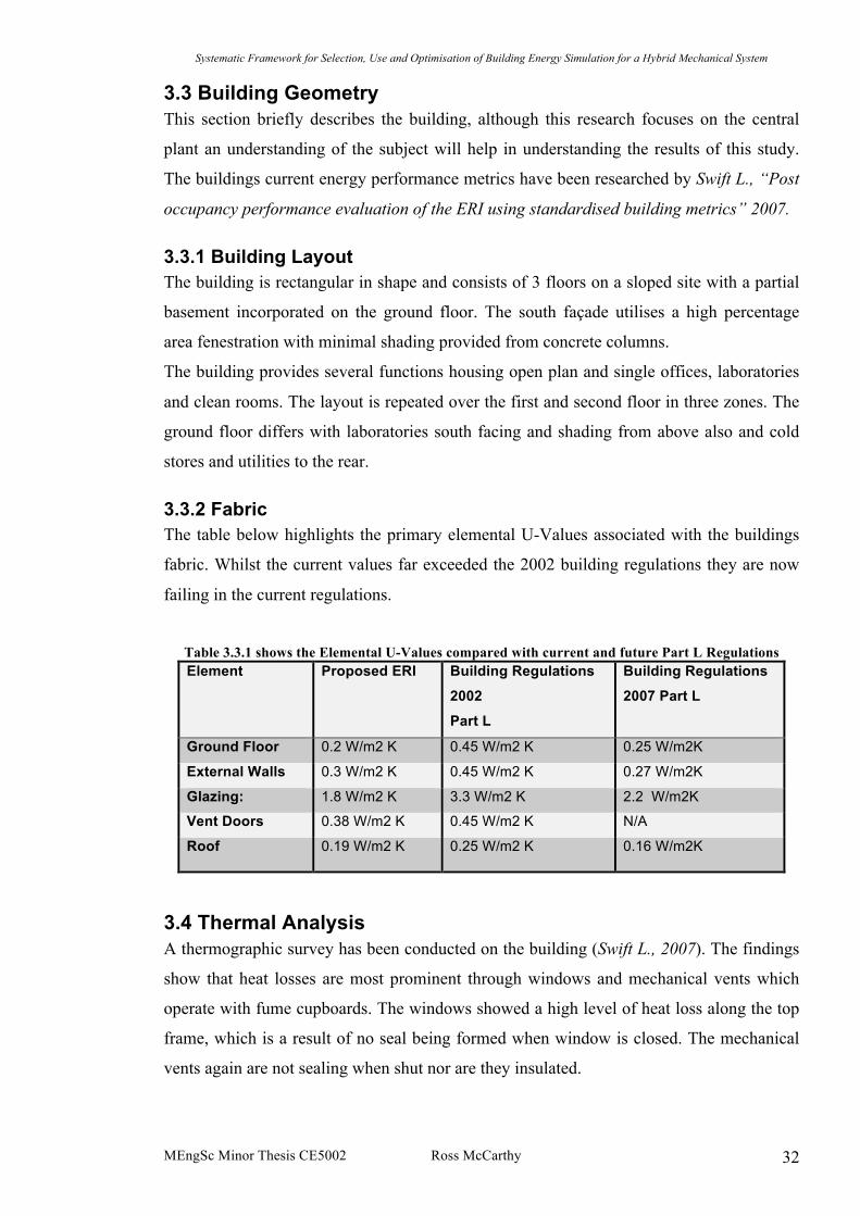
3.3.2 Fabric The table below highlights the primary elemental U-Values associated with the buildings
fabric. Whilst the current values far exceeded the 2002 building regulations they are now
failing in the current regulations.
Table 3.3.1 shows the Elemental U-Values compared with current and future Part L Regulations Element
Proposed ERI Building Regulations
2002
Part L
Building Regulations
2007 Part L
Ground Floor 0.2 W/m2 K 0.45 W/m2 K 0.25 W/m2K
External Walls 0.3 W/m2 K 0.45 W/m2 K 0.27 W/m2K
Glazing: 1.8 W/m2 K 3.3 W/m2 K 2.2 W/m2K
Vent Doors 0.38 W/m2 K 0.45 W/m2 K N/A
Roof
0.19 W/m2 K 0.25 W/m2 K 0.16 W/m2K
3.4 Thermal Analysis A thermographic survey has been conducted on the building (Swift L., 2007). The findings
show that heat losses are most prominent through windows and mechanical vents which
operate with fume cupboards. The windows showed a high level of heat loss along the top
frame, which is a result of no seal being formed when window is closed. The mechanical
vents again are not sealing when shut nor are they insulated.

Systematic Framework for Selection, Use and Optimisation of Building Energy Simulation for a Hybrid Mechanical System
MEngSc Minor Thesis CE5002 Ross McCarthy 33
3.5 BMS Data Required The simulation model will utilise data obtained from the BMS data archive for a 24hr
period in late November. This data was chosen as it represents a time when the central
plant operated closest to its envisaged design. An ideal scenario of utilising an annual set
of metrics is not possible due to mechanical plant failure and issues with the current BMS
system (see Appendix F).
The weather conditions for the period of simulation (fig 3.5.1) represents an ideal weekday
(Tuesday) from which to base the plants operation. With an average outside temperature of
10ºC and a minimum and maximum of 7.5 ºC and 13 ºC respectively, it is ensured that the
heating system will operate.
Outside temperature (21.Nov.06)
0
2
4
6
8
10
12
14
0 5 10 15 20 25 30
Time 24hrs
Out
side
Air
Tem
pera
ture
Figure 3.5 Outside Air Temperature for period of Simulation
The data obtained from the BMS data archive can be categorised into two groups from
which the basis of the model is formed. These groups are discussed in the following two
sections.
Systematic Framework for Selection, Use and Optimisation of Building Energy Simulation for a Hybrid Mechanical System
MEngSc Minor Thesis CE5002 Ross McCarthy 34
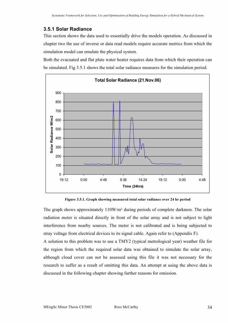
3.5.1 Solar Radiance This section shows the data used to essentially drive the models operation. As discussed in
chapter two the use of inverse or data read models require accurate metrics from which the
simulation model can emulate the physical system.
Both the evacuated and flat plate water heater requires data from which their operation can
be simulated. Fig 3.5.1 shows the total solar radiance measures for the simulation period.
Total Solar Radiance (21.Nov.06)
0
100
200
300
400
500
600
700
800
900
19:12 0:00 4:48 9:36 14:24 19:12 0:00 4:48
Time (24hrs)
Sol
ar R
adia
nce
W/m
2
Figure 3.5.1. Graph showing measured total solar radiance over 24 hr period
The graph shows approximately 110W/m² during periods of complete darkness. The solar
radiation meter is situated directly in front of the solar array and is not subject to light
interference from nearby sources. The meter is not calibrated and is being subjected to
stray voltage from electrical devices to its signal cable. Again refer to (Appendix F).
A solution to this problem was to use a TMY2 (typical metrological year) weather file for
the region from which the required solar data was obtained to simulate the solar array,
although cloud cover can not be assessed using this file it was not necessary for the
research to suffer as a result of omitting this data. An attempt at using the above data is
discussed in the following chapter showing further reasons for omission.
Systematic Framework for Selection, Use and Optimisation of Building Energy Simulation for a Hybrid Mechanical System
MEngSc Minor Thesis CE5002 Ross McCarthy 35
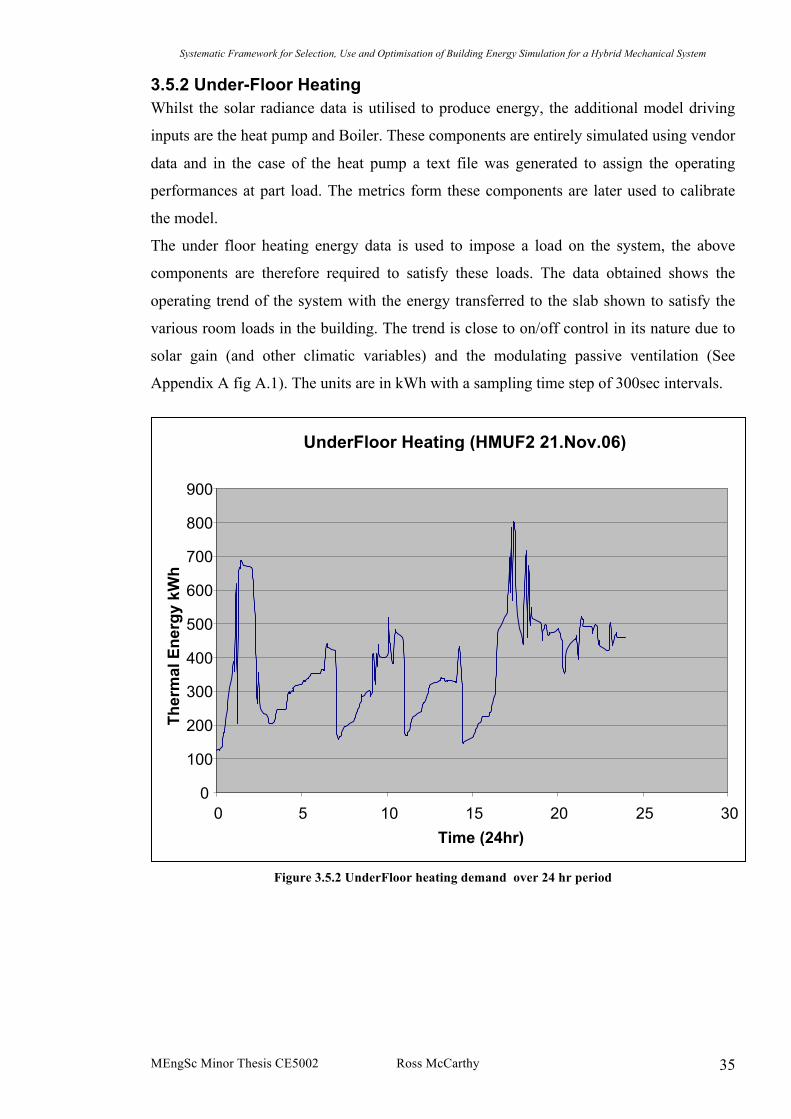
3.5.2 Under-Floor Heating Whilst the solar radiance data is utilised to produce energy, the additional model driving
inputs are the heat pump and Boiler. These components are entirely simulated using vendor
data and in the case of the heat pump a text file was generated to assign the operating
performances at part load. The metrics form these components are later used to calibrate
the model.
The under floor heating energy data is used to impose a load on the system, the above
components are therefore required to satisfy these loads. The data obtained shows the
operating trend of the system with the energy transferred to the slab shown to satisfy the
various room loads in the building. The trend is close to on/off control in its nature due to
solar gain (and other climatic variables) and the modulating passive ventilation (See
Appendix A fig A.1). The units are in kWh with a sampling time step of 300sec intervals.
Figure 3.5.2 UnderFloor heating demand over 24 hr period
UnderFloor Heating (HMUF2 21.Nov.06)
0
100
200
300
400
500
600
700
800
900
0 5 10 15 20 25 30 Time (24hr)
Ther
mal
Ene
rgy
kWh

Systematic Framework for Selection, Use and Optimisation of Building Energy Simulation for a Hybrid Mechanical System
MEngSc Minor Thesis CE5002 Ross McCarthy 36
3.5.3 AHU Heating Coils Both the under floor heating and AHU (Air Handling Unit) coils represent significant loads
imposed on the system. The graph below (fig 3.5.3) shows the least variable of the
imposed loads with a sustained demand over the simulated period. The AHU`s primarily
serve the laboratories located in the north facing rooms of the building. Again the units are
in kWh with a sampling time step of 300sec intervals.
These input files are contained in text files which are subsequently read using Type 9 data
readers linked to a load imposing component Type 682.
Figure 3.5.3 Graph showing AHU heating demand trend 24hr period
Air Handling Unit Heating Coils (HMUC1 21.Nov.06)
0
100
200
300
400
500
600
0 5 10 15 20 25 30 Time (24hrs)
Ther
mal
Ene
rgy
kWh

Systematic Framework for Selection, Use and Optimisation of Building Energy Simulation for a Hybrid Mechanical System
MEngSc Minor Thesis CE5002 Ross McCarthy 37
3.5.4 Hot Water Demand The final imposing input to the model is the demand for hot water. The profile shows a
sudden increase in the morning use and again drops suddenly at seven in the evening time.
The uniformity of this graph (fig 3.5.4) suggests a further analysis is warranted to ascertain
its validity. The base demand of 700 litres every 15 minutes during night-time is
unrealistic, however unlike the errors in solar radiance which were substituted with a
TMY2 this issue cannot be solved utilising synthetic data inputs. It has been found that the
hot water load is significantly higher than the design intent (Swift L., 2007)..
Figure 3.5.4 Graph showing hot water demand over 24hr period
3.5.5 Input Data Integrity As outlined, integrity issues pertaining to BMS have allowed a high level of uncertainty to
be associated with the simulations results once the simulation is run. Should the simulation
return favourable results, a process of validation will be required regardless. For the
simulation to truly emulate the plants operation, a set of manually measured or BMS
validated data represents an ideal scenario for this research.
Hot Water Demand
0
0.2
0.4
0.6
0.8
1
1.2
1.4
1.6
19:12 0:00 4:48 9:36 14:24 19:12 0:00 4:48 Time (24 hrs)
M^3
per
900
sec
900s
ec
Systematic Framework for Selection, Use and Optimisation of Building Energy Simulation for a Hybrid Mechanical System
MEngSc Minor Thesis CE5002 Ross McCarthy 38
3.5.6 Calibration Data
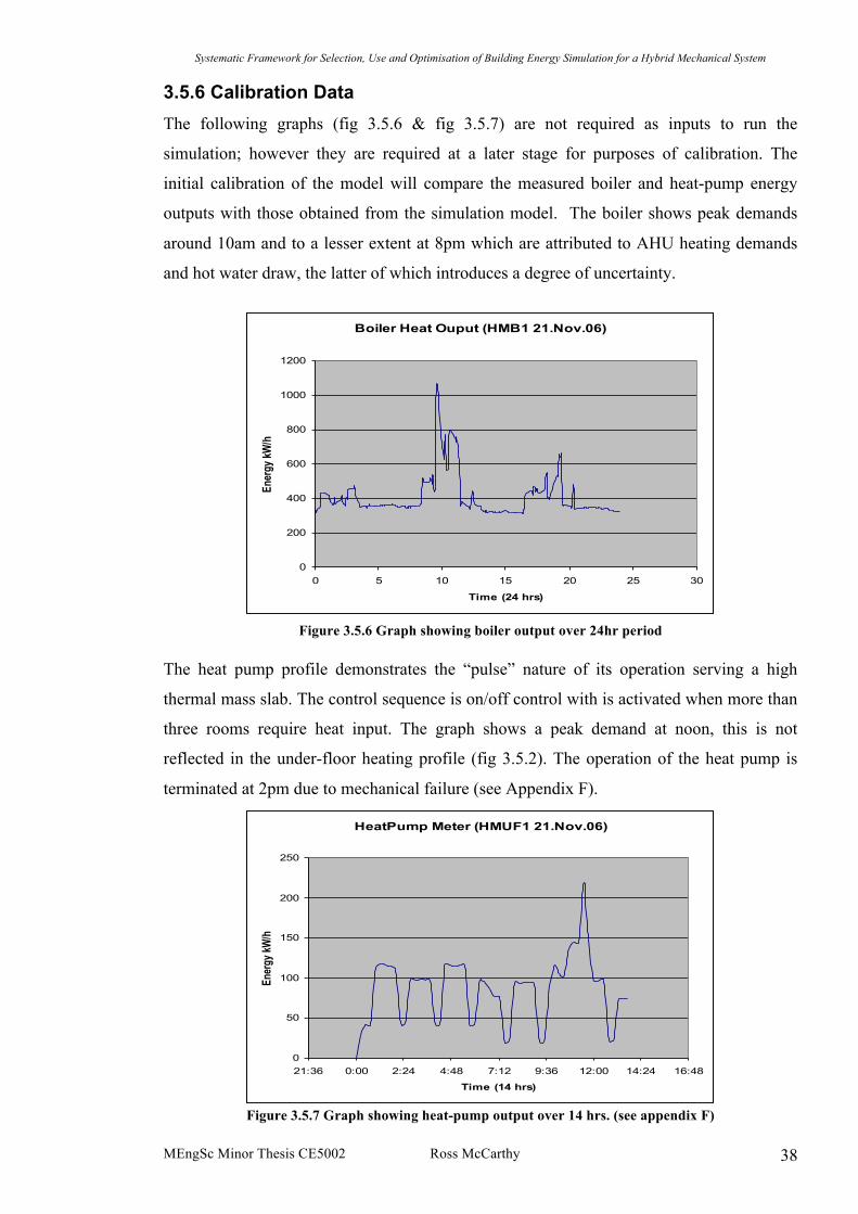
The following graphs (fig 3.5.6 & fig 3.5.7) are not required as inputs to run the
simulation; however they are required at a later stage for purposes of calibration. The
initial calibration of the model will compare the measured boiler and heat-pump energy
outputs with those obtained from the simulation model. The boiler shows peak demands
around 10am and to a lesser extent at 8pm which are attributed to AHU heating demands
and hot water draw, the latter of which introduces a degree of uncertainty.
Boiler Heat Ouput (HMB1 21.Nov.06)
0
200
400
600
800
1000
1200
0 5 10 15 20 25 30
Time (24 hrs)
Ener
gy kW
/h
Figure 3.5.6 Graph showing boiler output over 24hr period
The heat pump profile demonstrates the “pulse” nature of its operation serving a high
thermal mass slab. The control sequence is on/off control with is activated when more than
three rooms require heat input. The graph shows a peak demand at noon, this is not
reflected in the under-floor heating profile (fig 3.5.2). The operation of the heat pump is
terminated at 2pm due to mechanical failure (see Appendix F).
HeatPump Meter (HMUF1 21.Nov.06)
0
50
100
150
200
250
21:36 0:00 2:24 4:48 7:12 9:36 12:00 14:24 16:48
Time (14 hrs)
Energ
y kW/
h
Figure 3.5.7 Graph showing heat-pump output over 14 hrs. (see appendix F)
Systematic Framework for Selection, Use and Optimisation of Building Energy Simulation for a Hybrid Mechanical System
MEngSc Minor Thesis CE5002 Ross McCarthy 39
4 Model Outputs & Post Processing
Standard building simulation programs typically produce electrical demand and
consumption data as a program output. When modelling existing plants, if the results do
not match actual monitoring data, the programmer will typically “adjust” inputs and
operating parameters on a trial-and-error basis until the program output matches the
known data. This “fudging” process often results in the manipulation of a large number of
variables which may significantly decrease the credibility of the entire simulation
(Troncoso, 1997).
This chapter will discuss the initial runs, modifications and final outputs.
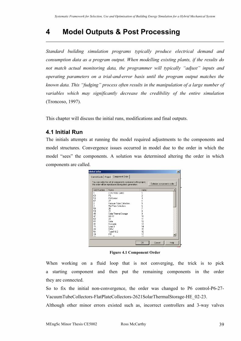
4.1 Initial Run The initials attempts at running the model required adjustments to the components and
model structures. Convergence issues occurred in model due to the order in which the
model “sees” the components. A solution was determined altering the order in which
components are called.
Figure 4.1 Component Order
When working on a fluid loop that is not converging, the trick is to pick
a starting component and then put the remaining components in the order
they are connected.
So to fix the initial non-convergence, the order was changed to P6 control-P6-27-
VacuumTubeCollectors-FlatPlateCollectors-2621SolarThermalStorage-HE_02-23.
Although other minor errors existed such as, incorrect controllers and 3-way valves
Systematic Framework for Selection, Use and Optimisation of Building Energy Simulation for a Hybrid Mechanical System
MEngSc Minor Thesis CE5002 Ross McCarthy 40
operating in on/off manner all of which were resolved. The initial run produced outputs
which would require post processing.
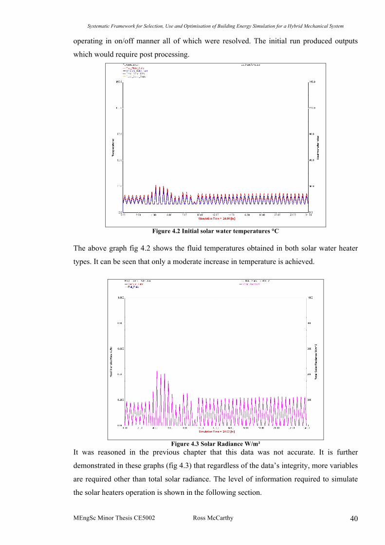
Figure 4.2 Initial solar water temperatures °C
The above graph fig 4.2 shows the fluid temperatures obtained in both solar water heater
types. It can be seen that only a moderate increase in temperature is achieved.
Figure 4.3 Solar Radiance W/m²
It was reasoned in the previous chapter that this data was not accurate. It is further
demonstrated in these graphs (fig 4.3) that regardless of the data’s integrity, more variables
are required other than total solar radiance. The level of information required to simulate
the solar heaters operation is shown in the following section.
Systematic Framework for Selection, Use and Optimisation of Building Energy Simulation for a Hybrid Mechanical System
MEngSc Minor Thesis CE5002 Ross McCarthy 41
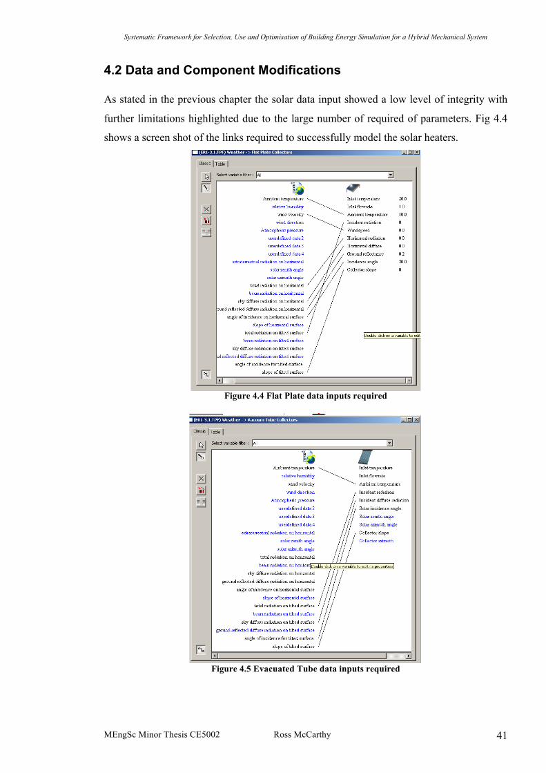
4.2 Data and Component Modifications As stated in the previous chapter the solar data input showed a low level of integrity with
further limitations highlighted due to the large number of required of parameters. Fig 4.4
shows a screen shot of the links required to successfully model the solar heaters.
Figure 4.4 Flat Plate data inputs required
Figure 4.5 Evacuated Tube data inputs required

Systematic Framework for Selection, Use and Optimisation of Building Energy Simulation for a Hybrid Mechanical System
MEngSc Minor Thesis CE5002 Ross McCarthy 42
4.3 Final Outputs AHU Coils: The final simulation results generated incorporate the necessary changes discussed
previously. Fig 4.6 shows the heat transfer rates kJ/hr (left axis) to both the AHU coils and
HE-04. Compared to the data obtained from the BMS the AHU coils profile shows slight
smoothening and follows the trend as expected. The transfer of heat to the heat exchanger
is significant as it demonstrates a period when the heat pump was unable to meet the load
imposed on the under floor heating.
Figure 4.6 Shows the Heat Transfer kJ/hr to the AHU Coils and HE-04 (Heatpump)

Systematic Framework for Selection, Use and Optimisation of Building Energy Simulation for a Hybrid Mechanical System
MEngSc Minor Thesis CE5002 Ross McCarthy 43
Boiler:
The profile shown in fig 4.7 shows both the boiler input and heat transferred to the quick
recovery vessel. The boiler burner is operated with on/off control and will therefore not
vary along the Y-axis (right). The frequency at which the boiler is called is signifgant
which is a result of a high demand from the hot water vessel. During this 24 hr period the
boiler is close to running consistently at full capacity.
Figure 4.7 Shows the Heat Transfer in kJ/hr from the Gas Boiler and to DHW.
The demand for hot water is shown on the left axis and denoted in kJ/hr. The initial peak is
as a result of the simulation starting from zero i.e., no thermal capacitance exists in the
system and therefore represents a cold start scenario
Systematic Framework for Selection, Use and Optimisation of Building Energy Simulation for a Hybrid Mechanical System
MEngSc Minor Thesis CE5002 Ross McCarthy 44
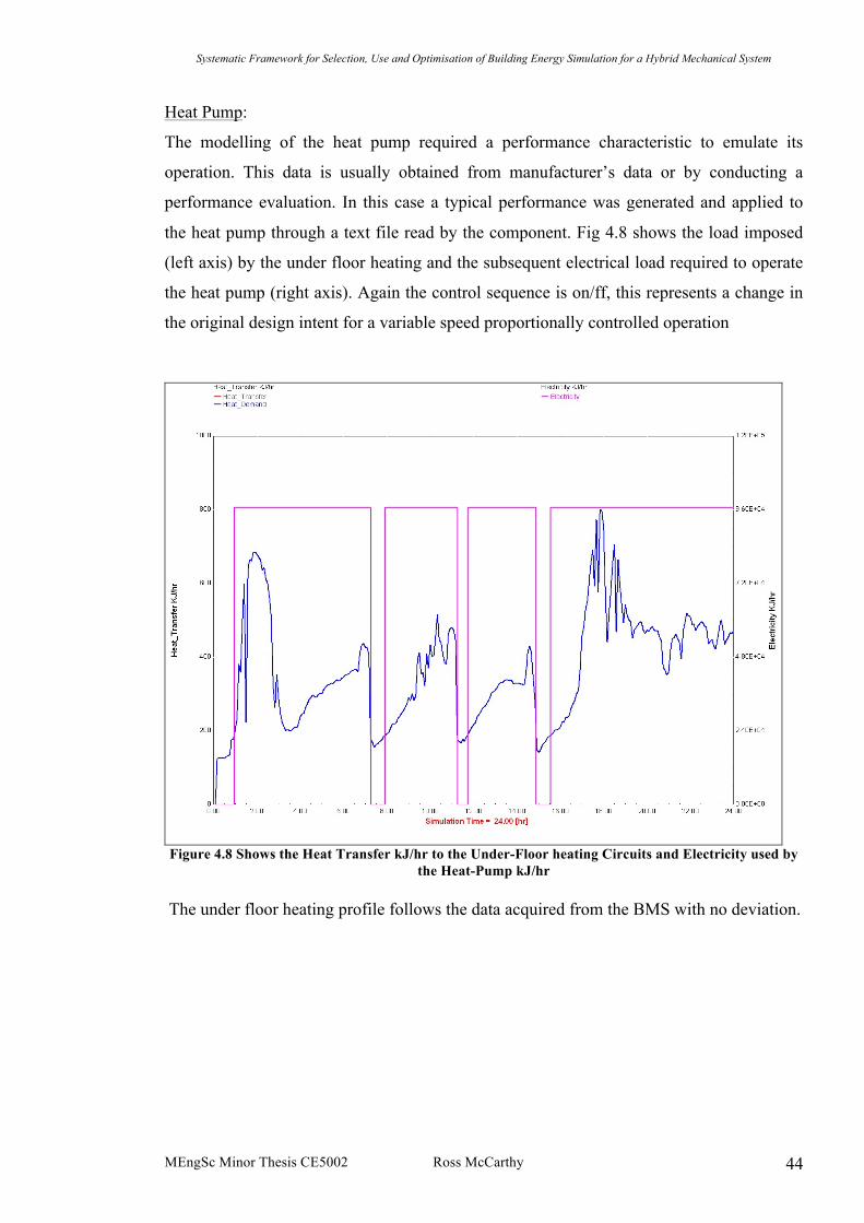
Heat Pump:
The modelling of the heat pump required a performance characteristic to emulate its
operation. This data is usually obtained from manufacturer’s data or by conducting a
performance evaluation. In this case a typical performance was generated and applied to
the heat pump through a text file read by the component. Fig 4.8 shows the load imposed
(left axis) by the under floor heating and the subsequent electrical load required to operate
the heat pump (right axis). Again the control sequence is on/ff, this represents a change in
the original design intent for a variable speed proportionally controlled operation
Figure 4.8 Shows the Heat Transfer kJ/hr to the Under-Floor heating Circuits and Electricity used by
the Heat-Pump kJ/hr The under floor heating profile follows the data acquired from the BMS with no deviation.

Systematic Framework for Selection, Use and Optimisation of Building Energy Simulation for a Hybrid Mechanical System
MEngSc Minor Thesis CE5002 Ross McCarthy 45
Hot Water:
As stated previously the demand for hot water is a significant energy use in the building.
The graph below (fig 4.9) shows the flow rate on the right axis against the heat transferred
into the vessel (same as fig 4.7). Uncertainties exist in this data which has had an effect on
the boiler output, essentially forcing the boiler operate at maximum potential.
Figure 4.9 Shows the Hot Water Demand m³/hr and Heat Transfer to Vessel kJ/hr

Systematic Framework for Selection, Use and Optimisation of Building Energy Simulation for a Hybrid Mechanical System
MEngSc Minor Thesis CE5002 Ross McCarthy 46
Solar Water Heaters:
The modelling of the solar array produced favourable results in terms of operation. The
trends follow closely to the solar data provided. The flat plate solar heater temperature is
shown in blue and the evacuated tube collectors shown in red (fig 4.10). As expected the
temperatures reached in the evacuated tubes exceeds the level reached the flat plate by
10°C.
The panels are operated with on/off control which is shown as a solid portion of the graph,
subsequent figures show this operation in greater detail.
Figure 4.10 Shows the Temperatures ºC in both Solar Water Heater Types

Systematic Framework for Selection, Use and Optimisation of Building Energy Simulation for a Hybrid Mechanical System
MEngSc Minor Thesis CE5002 Ross McCarthy 47
Figure 4.11 Vacuum Tube and Flat Plate Temperatures
Figure 4.12 Vacuum Tube Temperatures

Systematic Framework for Selection, Use and Optimisation of Building Energy Simulation for a Hybrid Mechanical System
MEngSc Minor Thesis CE5002 Ross McCarthy 48
Figure 4.13 Flat Plate Temperatures
Figure 4.14 Solar Buffer Vessel Heat Transfer kJ/hr

Systematic Framework for Selection, Use and Optimisation of Building Energy Simulation for a Hybrid Mechanical System
MEngSc Minor Thesis CE5002 Ross McCarthy 49
4.4 Model Calibration Due to integrity issues with the BMS data, it was not possible to adequately calibrate the
simulation model. Until these issues are resolved and validated it will not be possible to
develop this model as intended or can future research in this area pertaining to the ERI gain
recognition. The shortcomings of the BMS have therefore resulted in a lost opportunity for
this low energy research facility. The section will therefore outline the possible methods of
calibration when quality data can be obtained.
Building simulation tools have been used for testing retrofit/optimisation alternatives
worldwide. But the results provided by software would not be worth if the base case was
not correctly calibrated, i.e., the virtual model of the building under analysis must represent
faithfully the thermal and energy behaviour of that building or mechanical system. To
achieve this objective, one has to compare measured performance data with those values
predicted by the software. (Westphal, F.S, Lamberts, R. 2005).
Calibration levels are outlined in Table 4.1 Table 4.4.1 Proposed calibration levels as a function of input data available and time needed for
calibration (Maor et al., 2006) Calibration Levels
Building Description and performance data available for calibration Time needed for calibration
Energy
Invoices
(1yr)
As-built
drawings
Walk
through
site visit
Detailed
Audit*
Short-term
Monitored
end-use
data
Electrical
interval
data (1yr)
Long-term
monitored
data
Data
gathering
Analysis
(**)
Level 1 X X 30 min 1-2 hrs
Level 2 X X X 2-4 hrs 2-4 hrs
Level 3 X X X X 1-2
days
4-8 hrs
Level 4 X X X X X 2-3
days
1-2
days Level 5 X X X X X X 2-4 wks 2-4
days Level 6 X X X X X X X 4-6 mo. 6-10
days
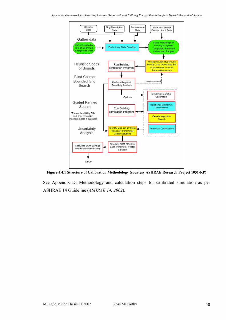
Systematic Framework for Selection, Use and Optimisation of Building Energy Simulation for a Hybrid Mechanical System
MEngSc Minor Thesis CE5002 Ross McCarthy 50
Figure 4.4.1 Structure of Calibration Methodology (courtesy ASHRAE Research Project 1051-RP)
See Appendix D: Methodology and calculation steps for calibrated simulation as per
ASHRAE 14 Guideline (ASHRAE 14, 2002).

Systematic Framework for Selection, Use and Optimisation of Building Energy Simulation for a Hybrid Mechanical System
MEngSc Minor Thesis CE5002 Ross McCarthy 51
5 Optimisation Methodology
Typically the optimisation of building energy simulation models is achieved through
experienced gained by the programmer, termed heuristic methods.
Heuristic methods make use of expert knowledge or experience gained by professionals
over the years in order to reach near optimal design (Maor et al., 2006). This approach
allows existing building simulation tools to be more effectively and efficiently used since it
reduces the number of competing system configurations to a relatively small set to which
detailed simulation tools can then be applied.
With the advent of more complex and innovative design solutions to building energy
systems, the isolation of individual components for optimisation is restrictive. A
mathematical approach is therefore considered.
5.1 Central Plant Optimisation In the case of the ERI, a number of components can interact to share loads and is
determined through a control strategy which was developed by BDP (Building Design
Partnership, Consultants). A calibrated simulation model can be used optimise this control
strategy, essentially challenging set points and storage vessels with priority designation.
Table 5.1 lists of plant systems (ERI) that have been identified as presenting opportunities for
optimisation. Application Controlled component Output to be optimised Optimum start/stop Heating component Start/stop time
Optimum set-back temperature Heating system Set-back temperature
Boiler/Heat-pump sequencing Boilers Heating system efficiency
Load shedding Heating system Priority for heating
Under-floor heating Heating system Hours of operation
Night operated ground water source heat
pumps
Water pump/compressor Start time
Solar control mode Controller Set points
Aquifer preheat from Solar Controller Set points
The above components can be optimised either for running cost reduction, CO2 emissions
reduction or a compromise of both.
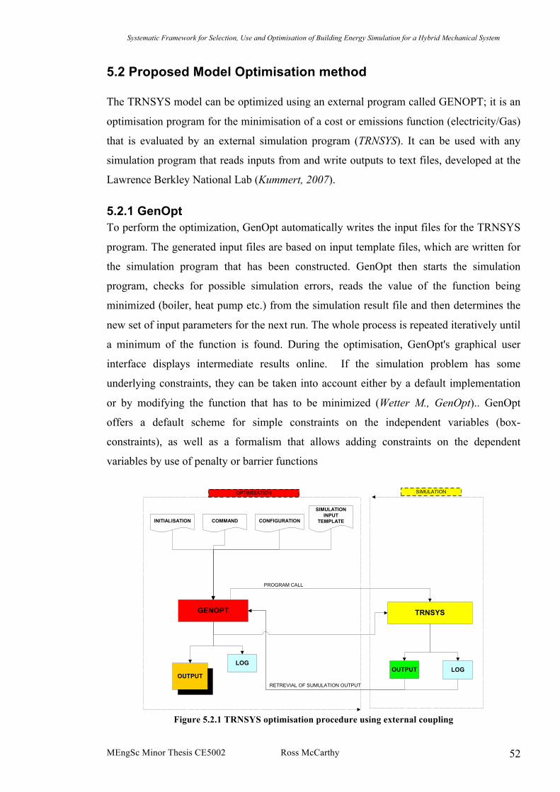
Systematic Framework for Selection, Use and Optimisation of Building Energy Simulation for a Hybrid Mechanical System
MEngSc Minor Thesis CE5002 Ross McCarthy 52
5.2 Proposed Model Optimisation method The TRNSYS model can be optimized using an external program called GENOPT; it is an
optimisation program for the minimisation of a cost or emissions function (electricity/Gas)
that is evaluated by an external simulation program (TRNSYS). It can be used with any
simulation program that reads inputs from and write outputs to text files, developed at the
Lawrence Berkley National Lab (Kummert, 2007).
5.2.1 GenOpt To perform the optimization, GenOpt automatically writes the input files for the TRNSYS
program. The generated input files are based on input template files, which are written for
the simulation program that has been constructed. GenOpt then starts the simulation
program, checks for possible simulation errors, reads the value of the function being
minimized (boiler, heat pump etc.) from the simulation result file and then determines the
new set of input parameters for the next run. The whole process is repeated iteratively until
a minimum of the function is found. During the optimisation, GenOpt's graphical user
interface displays intermediate results online. If the simulation problem has some
underlying constraints, they can be taken into account either by a default implementation
or by modifying the function that has to be minimized (Wetter M., GenOpt).. GenOpt
offers a default scheme for simple constraints on the independent variables (box-
constraints), as well as a formalism that allows adding constraints on the dependent
variables by use of penalty or barrier functions
LOGOUTPUT LOG
GENOPT TRNSYS
INITIALISATION COMMAND CONFIGURATION
SIMULATIONINPUT
TEMPLATE
OUTPUT
PROGRAM CALL
RETREVIAL OF SUMULATION OUTPUT
OPTIMISATION SIMULATION
Figure 5.2.1 TRNSYS optimisation procedure using external coupling
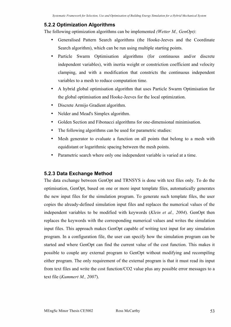
Systematic Framework for Selection, Use and Optimisation of Building Energy Simulation for a Hybrid Mechanical System
MEngSc Minor Thesis CE5002 Ross McCarthy 53
5.2.2 Optimization Algorithms The following optimization algorithms can be implemented (Wetter M., GenOpt):
• Generalised Pattern Search algorithms (the Hooke-Jeeves and the Coordinate
Search algorithm), which can be run using multiple starting points.
• Particle Swarm Optimisation algorithms (for continuous and/or discrete
independent variables), with inertia weight or constriction coefficient and velocity
clamping, and with a modification that constricts the continuous independent
variables to a mesh to reduce computation time.
• A hybrid global optimisation algorithm that uses Particle Swarm Optimisation for
the global optimisation and Hooke-Jeeves for the local optimization.
• Discrete Armijo Gradient algorithm.
• Nelder and Mead's Simplex algorithm.
• Golden Section and Fibonacci algorithms for one-dimensional minimisation.
• The following algorithms can be used for parametric studies:
• Mesh generator to evaluate a function on all points that belong to a mesh with
equidistant or logarithmic spacing between the mesh points.
• Parametric search where only one independent variable is varied at a time.
5.2.3 Data Exchange Method The data exchange between GenOpt and TRNSYS is done with text files only. To do the
optimisation, GenOpt, based on one or more input template files, automatically generates
the new input files for the simulation program. To generate such template files, the user
copies the already-defined simulation input files and replaces the numerical values of the
independent variables to be modified with keywords (Klein et al., 2004). GenOpt then
replaces the keywords with the corresponding numerical values and writes the simulation
input files. This approach makes GenOpt capable of writing text input for any simulation
program. In a configuration file, the user can specify how the simulation program can be
started and where GenOpt can find the current value of the cost function. This makes it
possible to couple any external program to GenOpt without modifying and recompiling
either program. The only requirement of the external program is that it must read its input
from text files and write the cost function/CO2 value plus any possible error messages to a
text file (Kummert M., 2007).

Systematic Framework for Selection, Use and Optimisation of Building Energy Simulation for a Hybrid Mechanical System
MEngSc Minor Thesis CE5002 Ross McCarthy 54
5.2.4 TRNOPT (TRNSYS) Recent developments amongst the TRNSYS developer group have improved the link
between GenOpt and TRNSYS with a dedicated component called TRNOPT which can
call the program seamlessly into the model. Essentially TRNOPT is a dedicated TRNSYS
interface for GENOPT. It was been created by TESS (Thermal Energy Systems
Specialists) in order to streamline the optimisation process and it is distribute as part of the
TRNSYS library. With TRNOPT, the entire process of optimising the results from a
TRNSYS simulation reduces to choosing the TRNSYS input file, choosing the variables
which will be varied to optimise the results, and choosing the simulation result to be
optimised.
Systematic Framework for Selection, Use and Optimisation of Building Energy Simulation for a Hybrid Mechanical System
MEngSc Minor Thesis CE5002 Ross McCarthy 55
6 Conclusion
This research project has put in place framework for building energy simulation tools that
were assessed in their ability to simulate a hybrid complex system. The procedure allowed
for an effective initial selection from twenty leading programs. From this, a final review of
the most capable tools was established, this included the following programs:
ESP-r, EnergyPLUS, IDA ICE, TRNSYS and SimBad.
TRNSYS was determined to offer the most capable ability to complete the task of
simulating the ERI central mechanical plant. Funding was secured for purchase of the
program from the National University of Ireland “Green Building Fund”.
The model was implemented over a period of eight weeks, a detailed knowledge of the
capabilities and possibilities of the program were gained during this time. Obstacles were
resolved timely and effectively with expert advice from TRNSYS developers. The
challenge of emulating the control strategy was overcome using a sequence of “trial and
error” on an array of controllers in the program library. A combination of proportional and
on/off controllers was determined to over the most realistic virtual representation of the
physical system.
It has been acknowledged, that obstacles in developing a complex model such as this
required a different approach. The central plant required the simulation of three main
systems (Boiler, Solar heaters and a Heat-pump). These systems should have in hindsight
been simulated separately to begin with, allowing minimal errors when the systems are
subsequently joined. This approach is effectively a time saving method.
The importance of accurate and calibrated data for this inverse method of simulation is
paramount. Integrity issues with the BMS have introduced uncertainties to the generated
model results, in terms of calibrated simulation work on this building the present time
represents an opportunity lost. The future works emanating from this model is essentially a
waiting game until such time that the BMS issues are resolved and metrics collected.
A procedure for evaluating optimisation potential was outlined in Chapter 6. Once the
model is calibrated this mathematical mode of determining optimum set points for plant
operation can be implemented. The theory of this procedure was discussed; it showed that
this form of optimisation is not limited to plant systems complex or otherwise. It highlights

Systematic Framework for Selection, Use and Optimisation of Building Energy Simulation for a Hybrid Mechanical System
MEngSc Minor Thesis CE5002 Ross McCarthy 56
a method for whole building optimisation for design stage, operational stage and retrofit
evaluation. Methods of whole building simulation are outlined in Appendix A which
includes co-simulation amongst current models of the ERI.
Future works dependent upon this model are outlined in Appendix A, which expands on
the initial diagram fig 1.1 showing the possibilities of attainable upon completion of this
model.
As reported in the introduction the energy use in the built environment represent 40% of
the energy use in the EU (EU Directive 2006/32/EC). The challenges in reducing the
energy used in our current building stock is somewhat overlooked with modern more
energy efficient building becoming mandatory distracting policy makers from updating the
current built environment.
Systematic Framework for Selection, Use and Optimisation of Building Energy Simulation for a Hybrid Mechanical System
MEngSc Minor Thesis CE5002 Ross McCarthy 57
Acknowledgements
I wish to thank the following people for their guidance and help in completing this
research.
• Dr. Marcus Keane, IRUSE (Civil and Environmental Engineering Department)
• James O’Donnell, IRUSE, PhD Student
• David Bradley, Thermal Energy System Specialists (TESS), Madison, Wisconsin,
USA.
• Tim O`Riordan, Thermal Energy System Specialists (TESS), Madison, Wisconsin,
USA.
• Jeff Thornton, Thermal Energy System Specialists (TESS), Madison, Wisconsin,
USA.
I would also like to acknowledge the efforts of the TRNSYS Developers Group.
• The Solar Energy Laboratory at the University of Wisconsin-Madison, USA.
• The Centre Scientifique et technique du Bâtiment in Nice, France.
• Transsolar Energietechnik GmBH in Stuttgart, Germany.
Systematic Framework for Selection, Use and Optimisation of Building Energy Simulation for a Hybrid Mechanical System
MEngSc Minor Thesis CE5002 Ross McCarthy 58
References
Crawley D, Hand J, Kummert M, Griffth B, 2005 Contrasting the Capabilities of Building Energy Performance Simulation Programs Clarke J, 2001. Energy Simulation in Building Design, 2nd Edition Energy Systems Research Unit 2002. The ESP-r System for Building Energy Simulation, User Guide Version 10 Series Fong K.F., Hanby V.I., Chow T.T., 2005, HVAC system optimization for energy management by evolutionary programming, Hong Kong Trcka M, Hensen J, Tschnische Universities Eindhoven, 2005, Model and Tool Requirements for Co-Simulation of Building Performance. Riederer P, Couilland N. 2003 Improving HVAC systems using the SIMBAD HVAC and Building toolbox: form sizing and control to performance assessment, ISPRA conference, Ispra, Italy. Riederer P, 2005 MatLab/Simulink for Building and HVAC Simulation –State of the Art. Riederer P., et al. 2001, Development and quality improvements of HVAC control systems in virtual laboratories. Riederer P., et al. 2000. Building zone modeling adapted to the study of temperature control systems, ASHRAE/CIBSE 2000, Dublin, Ireland. De Wit M.H, 2001, WaVo, A Simulation Model for the Thermal and Hygric Performance of a Building. Deque F., Noel J., Roux J.J. 2001 SISLEY: An open tool for transient state
two dimensional heat transfer. 7th International IBSPA Conference, Rio de Janeiro, Brazil, 2001. Peng X. 1996. Modelling of indoor thermal conditions for comfort control in buildings, PhD thesis, Delft, University of Technology. Peng X., van Passen 1997 Simplified modeling of indoor dynamic temperature distributions, Clima2000, Brussels. Simbad, 2004. SIMBAD Building and HVAC Toolbox, CSTB. Stec W., van Passen D. 2003 Defining the performance of the double skin facade with the use of the simulation model, ISPSA 2003. Park et al. 2003. Daylighting optimization in smart façade systems IPBSA 2003 Yu et al. 2003. Fuzzy neural networks model for building energy diagnosis IPBSA 2003 Yu et al. 2003. Modelling analysis on fin tube heating coil of air handling unit BSERT Husaunndee A., Riederee P., Visier J.C 1998, Coil modelling in the SIMBAD Toolbox-Numerical and experimental validation of the cooling coil model. SSB 1998. Jain D., Tiwari G.N 2003., Modelling and optimal design of ground air collector for heating in controlled environment greenhouse. Kumara R., Kaushik S.C 2005 Performance evaluation of green roof and shading for thermal protection of buildings, Building and Environment.
Systematic Framework for Selection, Use and Optimisation of Building Energy Simulation for a Hybrid Mechanical System
MEngSc Minor Thesis CE5002 Ross McCarthy 59
Klein, et al., TRNSYS- A Transient System Simulation Program User Manual, Wisconsin 2005. Boer C.A, 2005 Distributed simulation in industry, PhD thesis, Rotterdam Ganse A. 2005, Distributed processing, University of Washington, Seattle. Fujimoto R.M 2005 Parallel and distributed simulation- introduction and motivation, Georgia institute of technology, College of Computing. Janak M., 1997, Coupling building energy and lighting simulation, IPBSA Prague. Djunaedy E., Hensen J.L.M., 2003, Towards external coupling of building energy and air flow modeling programs, ASHRAE Transactions Zhai Z., 2004 Developing and integrated building design tool by coupling building energy simulation and computational fluid dynamics program, PhD Thesis, Massachusetts Institute of Technology Hensen J.L.M., 1999, A comparison of coupled and decoupled solutions for temperature and air flow in a building, ASHRAE Transactions. Kelly G.E., May W., Kao J., 1994 Using emulators to evaluate the performance of building energy management systems, ASHRAE Transactions. Haves P., Norford L.K., DeSimone M., 1998, A standard simulation test bed for the evaluation of control algorithims and strategies, ASHRAE Transactions. Clarke J., Cockroft J., Conner S., Hand J., Kelly., Moore R., O`Brien T., Strachan P., 2002, Simulation-assisted control in
building energy management systems, ESRU Strathclyde, Glasgow and Honeywell Control Systems, Motherwell UK. Martin A., Banyard C., 1998 Library of system control strategies, BSRIA application guide. Kummert M., 2007, Using GenOpt with TRNSYS 16 and Type 56, ESRU-University of Strathclyde. Klein et al., 2004, TRNSYS 16 – A transient system simulation program, user manual, solar energy lab, University of Wisconsin. Wetter M. GenOpt 2004, Generic optimization program, user manual, version 2.0.0, Lawrence Berkley National Laboratory. Stein, 1997 Energy System Laboratory of Texas A&M University TESS, 2004. TRNOPT v16, Thermal Energy System Specialists, Madison, WI. Troncoso, R., 1997. “A hybrid monitoring-modeling procedure for analyzing the performance of large central chilling plants”, IBPSA Conference Proceedings, Prague, Czech Republic. Maor I., Reddy T. A., 2006, “Procedures for Reconciling Computer-Calculated Results with Measured Energy Data”, ASHRAE Research Project 1051-RP. Swift L,. 2007 “Post occupancy performance evaluation of the ERI using standardised building metrics.” Sustainable Energy Masters Minor Research Thesis.
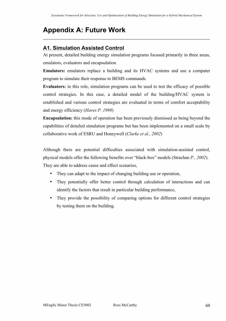
Systematic Framework for Selection, Use and Optimisation of Building Energy Simulation for a Hybrid Mechanical System
MEngSc Minor Thesis CE5002 Ross McCarthy 60
Appendix A: Future Work
A1. Simulation Assisted Control At present, detailed building energy simulation programs focused primarily in three areas,
emulators, evaluators and encapsulation
Emulators: emulators replace a building and its HVAC systems and use a computer
program to simulate their response to BEMS commands.
Evaluators: in this role, simulation programs can be used to test the efficacy of possible
control strategies. In this case, a detailed model of the building/HVAC system is
established and various control strategies are evaluated in terms of comfort acceptability
and energy efficiency (Haves P. 1998)
Encapsulation: this mode of operation has been previously dismissed as being beyond the
capabilities of detailed simulation programs but has been implemented on a small scale by
collaborative work of ESRU and Honeywell (Clarke et al., 2002)
Although there are potential difficulties associated with simulation-assisted control,
physical models offer the following benefits over “black-box” models (Strachan P., 2002).
They are able to address cause and effect scenarios,
• They can adapt to the impact of changing building use or operation,
• They potentially offer better control through calculation of interactions and can
identify the factors that result in particular building performance,
• They provide the possibility of comparing options for different control strategies
by testing them on the building.

Systematic Framework for Selection, Use and Optimisation of Building Energy Simulation for a Hybrid Mechanical System
MEngSc Minor Thesis CE5002 Ross McCarthy 61
A1.1 Observed problem The need of forecasting is shown in Fig4.1 showing the temperature profile in ERI room
G24 (it was not possible to obtain figures form heat flow meter). This situation can be
encountered in a passive solar
building with large south-facing
windows. If there is no cooling plant,
overheating can occur during a sunny
afternoon, despite the fact that
heating has been required in the
morning.
If overheating occurs then it is too
late to take a control decision for the
heating plant: the heat stored in the
building structure cannot be removed. Fig A1.1 ERI Open Office G24
A reduction of energy consumption would have certainly been achieved if the temperature
rise had been forecasted, in order to prevent unnecessary heating during the morning hours.
Open office Temperature Profile
19
20
21
22
23
24
25
Time
Time (3Hrs)
Tem
pera
ture
oC

Systematic Framework for Selection, Use and Optimisation of Building Energy Simulation for a Hybrid Mechanical System
MEngSc Minor Thesis CE5002 Ross McCarthy 62
A1.2 Possible Solution-Model Predict
MATLABSIMULINK
COMMONDATABASE
IES/ENERGY
PLUS
PREDICTEDWEATHER DATA
(4HR)
CYLON BMSHISTORICAL
DATA
RESTRICT BMS @BUFFER VESSEL
EFFECTIVNESSRATIO
IDEALISEDENERGYUSE KWh
4HR MEASUREDENERGY USE KWh
Weather data transmitted toprogram via Web Link.
These would ideally forecast4hr temperatures, wind
speed and precipatation.
Building Loads generatedusing simulation software willsupplement the actual data
measured during early life ofthe building. These blockloads may be overwritten.
The ideal energy use wouldbe determined from a setcriteria established using
BREEAM at early stage ofdesign.
The recorded energy use willbe benchmarked against the
idealised. An effectivnessratio will be calculated. Thisratio will be used to prioritise
the block loads in thedatabase.
Hourly block loads arestored in matlab. These
blocks correspond to specificexternal weather. Intially
generated using software butreplaced by measured loads.
A signal will issue acommand of yes or no
overriding the Underfloorheating pumps.
CYLONBMS
MOTORCONTROL
PANEL
Figure A1.2 Flow Chart of the possible simulation environment
The initial investigation of determining what figures can be obtained from MET Eireann
showed it was not possible to gain accurate outlooks when temperatures are required.
Following correspondence with the MET office it was decided that this method would
need a general outlook for the day along with historical weather data from the ERI to be
able to generate useful results.
“We can provide the historical data from April 2006 to date, however we do not have a
service that allows you to download 4 hourly figures from our website, once the
observations are collected each hour, it takes at least a day for the hourly observations to
be entered into the database, quality controlled and then made available to customers”.
It is currently an entire research area in itself (Ensemble Prediction, Lang S. 2007)

Systematic Framework for Selection, Use and Optimisation of Building Energy Simulation for a Hybrid Mechanical System
MEngSc Minor Thesis CE5002 Ross McCarthy 63
A1.3 Possible Solution-A Neural Network Controller (ANN) A neural network controller has previously implemented in a similar solar building for
implementation in a hydronic heating system (Argiriou A., et al 2003). The controller had
forecasting capabilities: it included a meteorological module, forecasting the ambient
temperature and solar irradiance, an indoor temperature predictor module, a supply
temperature predictor module and an optimizing module for the water supply temperature.
All ANN modules were based on the Feed Forward Back Propagation (FFBP) model.
In was concluded from this experiment (two rooms) that the ANN controller leads to 18%
of energy savings over the test period with respect to the conventional one. Simulations
showed that energy savings over the heating season range from 13 to 17%, depending on
the heating schedule used.
Figure A1.3 Implemented ANN controller (Argiriou A., et al 2003)
Systematic Framework for Selection, Use and Optimisation of Building Energy Simulation for a Hybrid Mechanical System
MEngSc Minor Thesis CE5002 Ross McCarthy 64
Appendix B Reviewed Software Capabilities See CD
Appendix C: Previous ERI Simulation work
Problems Encountered: EnergyPlus
Previous efforts of using EnergyPlus to create a dynamic model the ERI building as a
whole have encountered problems. As reported by Elmer Morrisey the airside system
modelling posed the greatest difficultly, primarily due to the mass balance approach
applied to air loops as employed by EnergyPlus. This method is incapable of modelling
rooms or zones that require positive or negative pressure in relation to adjacent rooms.
This is particularly evident in the laboratory areas which require pressure differences for
containing cross contamination; to a lesser extent the toilet areas need a similar approach.
The natural ventilation could not be modelled either as EnergyPlus lacks this ability.
Therefore, at present a working dynamic model of the building as a whole does not exist. It
was therefore concluded that the mechanical and passive air system could not be modelled
with this software at present.
Problems also arose with the waterside modelling as the complex control strategy proved
to complex for EnergyPlus to emulate.
As a mixed use low energy building, the laboratory aspects of the building coupled with
passive elements has proved difficult to simulate. Previous findings have similarly
concluded that it is notoriously difficult to effectively moderate low levels of energy use in
laboratory facilities (Federspiel, Zhang et al. 2002).
Despite the above problems it is the authors opinion the EnergyPlus model could be
salvaged utilising co-simulation i.e., coupling the building thermal load model
(EnergyPlus) with a plant model either MatLab/SimLink (SimBad) or TRNSYS.

Systematic Framework for Selection, Use and Optimisation of Building Energy Simulation for a Hybrid Mechanical System
MEngSc Minor Thesis CE5002 Ross McCarthy 65
Appendix D: Calibration Procedures
Methodology and calculation steps for calibrated simulation as per ASHRAE 14 Guideline (taken from ASHRAE 14, 2002) 1) Produce a calibrated simulation plan. Before a calibrated simulation analysis may begin, several
questions must be answered. Some of these questions include: Which software package
will be applied? Will models be calibrated to monthly or hourly measured data, or both? What
are to be the tolerances for the statistical indices? The answers to these questions are documented in
a simulation plan.
2) Collect data. Data may be collected from the building during the baseline period, the retrofit
period, or both. Data collected during this step includes dimensions and properties of building
surfaces, monthly and hourly whole-building utility data, nameplate data from HVAC and other
building system components, operating schedules, spot-measurements of selected HVAC and
other building system components, and weather data.
3) Input data into simulation software and run model. Over the course of this step the data
collected in the previous step is processed to produce a simulation-input file. Modelers are
advised to take care with zoning, schedules, HVAC systems, model debugging (searching for and
eliminating any malfunctioning or erroneous code), and weather data.
4) Compare simulation model output to measured data. The approach for this comparison varies
depending on the resolution of the measured data. At a minimum, the energy flows projected by
the simulation model are compared to monthly utility bills and spot measurements. At best, the
two data sets are compared on an hourly basis. Both graphical and statistical means may be used
to make this comparison.
5) Refine model until an acceptable calibration is achieved. Typically, the initial comparison
does not yield a match within the desired tolerance. In such a case, the modeler studies the
anomalies between the two data sets and makes logical changes to the model to better match the
measured data. The user should calibrate to both pre- and post-retrofit data wherever possible
and should only calibrate to post-retrofit data alone when both data sets are absolutely
unavailable. While the graphical methods are useful to assist in this process, the ultimate
determination of acceptable calibration will be the statistical method.
6) Produce baseline and post-retrofit models. The baseline model represents the building, as it
would have existed in the absence of the energy conservation measures. The retrofit model
represents the building after the energy conservation measures are installed. How these models
are developed from the calibrated model depends on whether a simulation model was calibrated
to data collected before the conservation measures were installed, after the conservation measures
were installed, or both times. Furthermore, the only differences between the baseline and
postretrofit models must be limited to the measures only. All other factors, including weather and
occupancy must be uniform between the two models unless a specific difference has been

Systematic Framework for Selection, Use and Optimisation of Building Energy Simulation for a Hybrid Mechanical System
MEngSc Minor Thesis CE5002 Ross McCarthy 66
observed that must be accounted for.
7) Estimate savings. Savings are determined by calculating the difference in energy flows and
intensities of the baseline and post-retrofit models using the appropriate weather file.
8) Report on observations and savings. Savings estimates and observations are documented in a
reviewable format. Additionally, sufficient model development and calibration documentation
shall be provided to allow for accurate recreation of the baseline and post-retrofit models by
informed parties, including: input and weather files.

Systematic Framework for Selection, Use and Optimisation of Building Energy Simulation for a Hybrid Mechanical System
MEngSc Minor Thesis CE5002 Ross McCarthy 67
Appendix E: Co-Simulation Methods
E.1 Co-Simulation/Coupling Current building energy simulation tool have to an extent been surpassed by complex
buildings in terms of shape, layout, functionality and services. The requirements for
flexibility and adaptability have increased, as has been experienced by previous attempts of
whole building simulation models in the ERI case. An efficient way forward would be to
share developments and to reuse existing component models. This approach can therefore
best take advantage of advances in various programs to benefit the model as a whole, i.e. to
use the best simulation model available without being limited.
E.1.1 External Coupling
The external coupling approach brakes the boundaries between different simulations and
by that introduces the potential to pool resources. Compared to the traditional approach,
external coupling generates several advantages (Boer C.A., 2005),(Ganse A.,
2005),(Fujimoto., 2005),
o reusability of already existing (legacy) software,
o combination of heterogeneous technologies,
o collaborative model design and development process,
o information hiding,
o scalability and fault tolerance
o geographically distributed components, and
o potentially reducing model execution time & more available memory.
Some software-specific work has been done by others regarding the external coupling in
the field of building performance simulation in general such as;
o ESP-r and Radiance (Janak M., 1997)
o ESP-r and Fluent (Djunaedy E., 2003)
o EnergyPlus and MIT-CFD (Zhai Z., 2004)
In addition to the general to the above there has been several developments regarding co-
simulation in the domain of HVAC systems and control. For example TRNSYS developers
introduced a type 155, defined a MatLab connection. Matlab is launched at every TRNSYS
time step as a separate process. The type 155 communicates with the MatLab engine
Systematic Framework for Selection, Use and Optimisation of Building Energy Simulation for a Hybrid Mechanical System
MEngSc Minor Thesis CE5002 Ross McCarthy 68
through a component object model interface. Any MatLab/Simulink can be run within
TRNSYS (Bradley D. 2005). The latest version of TRNSYS 14.0 has essentially made this
link transparent.
These efforts within the building simulation domain show a great need for interoperable
simulation environments.
E1.2 Coupling Strategy
There are two different coupling strategies (Hensen J.L.M 1999),
• Ping-pong coupling, and
• Onion coupling
With ping-pong coupling, distributed models run in sequence, where each model uses the
known (from the previous time step calculation) output values of the coupled model.
Whilst onion-coupling strategy requires that models iterate within each time step until the
difference between the calculated and estimated values falls within a specified predefined
tolerance.
However, it has been shown that for a sufficiently small coupling time step, both of these
strategies give the same results. There is only one information exchange between the
coupled programs in each direction per simulation time step.
E1.3 Coupling TRNSYS and IES
To allow for such a model to be created in TRNSYS simulations the developers have
created components in the TRNSYS code that explicitly link to the external programs,
execute the models and provide some method of data transfer between the programs.
Currently links have been created for Engineering Equation Solver (EES) (Klein 2004),
MATLAB™ and Simulink™ (Mathworks 2003), and Microsoft Excel™ (Microsoft 2004).
These components work by having TRNSYS call the external program at each iteration
and executing the model in its program. The results are then passed back to TRNSYS
where they can be used in a TRNSYS simulation like any other results from a standard
component.
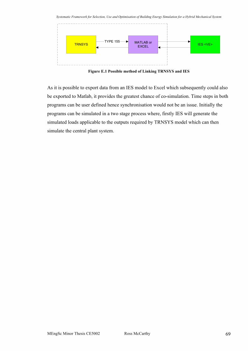
Systematic Framework for Selection, Use and Optimisation of Building Energy Simulation for a Hybrid Mechanical System
MEngSc Minor Thesis CE5002 Ross McCarthy 69
TRNSYS MATLAB orEXCEL IES <VE>
TYPE 155
Figure E.1 Possible method of Linking TRNSYS and IES
As it is possible to export data from an IES model to Excel which subsequently could also
be exported to Matlab, it provides the greatest chance of co-simulation. Time steps in both
programs can be user defined hence synchronisation would not be an issue. Initially the
programs can be simulated in a two stage process where, firstly IES will generate the
simulated loads applicable to the outputs required by TRNSYS model which can then
simulate the central plant system.
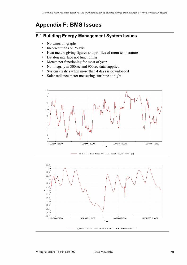
Systematic Framework for Selection, Use and Optimisation of Building Energy Simulation for a Hybrid Mechanical System
MEngSc Minor Thesis CE5002 Ross McCarthy 70
Appendix F: BMS Issues
F.1 Building Energy Management System Issues • No Units on graphs • Incorrect units on Y-axis • Heat meters giving figures and profiles of room temperatures • Datalog interface not functioning • Meters not functioning for most of year • No integrity in 300sec and 900sec data supplied • System crashes when more than 4 days is downloaded • Solar radiance meter measuring sunshine at night
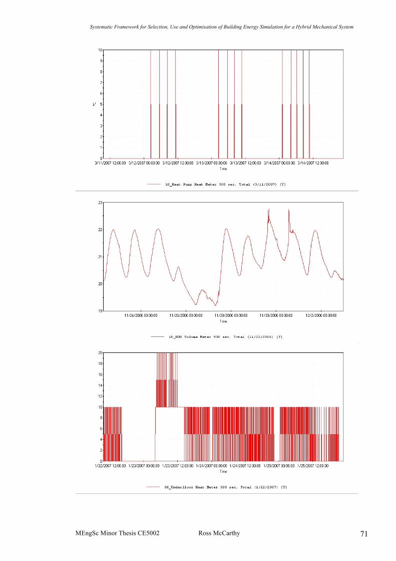
Systematic Framework for Selection, Use and Optimisation of Building Energy Simulation for a Hybrid Mechanical System
MEngSc Minor Thesis CE5002 Ross McCarthy 71

Systematic Framework for Selection, Use and Optimisation of Building Energy Simulation for a Hybrid Mechanical System
MEngSc Minor Thesis CE5002 Ross McCarthy 72
Appendix G: Simulation File
See CD


![Optimisation of autofrettage in thick- walled cylindersshuman/NEXT/MATERIALS&COMPONENTS... · Brownell and Young [7], and Yu [8] proposed a repeated trial calculation method to determine](https://img.pdfslide.us/doc/110x75/5b0de7fd7f8b9ab7658d2881/optimisation-of-autofrettage-in-thick-walled-cylinders-shumannextmaterialscomponentsbrownell.jpg)