Embed Size (px)
Citation preview

NASA Technical Paper 1804
Solar Power Satellite System Sizing Tradeoffs
G. D. Arndt and L. G. Monford
FEBRUARY 198 1
c . 1 1- ’
I
h
https://ntrs.nasa.gov/search.jsp?R=19810009968 2018-05-31T04:49:52+00:00Z

TECH LIBRARY KAFB, NM
NASA Technical Paper 1804
Solar Power Satellite System Sizing Tradeoffs
G. D. Arndt and L. G. Monford Lyudon B. Johtzsou Space Celzter Houston, Texas
National Aeronautics and Space Administration
Scientific and Technical Information Branch
1981
I
I
CONTENTS
Section Page
INTRODUCTION . . . . . . . . . . . . . . . . . . . . . . . . . . . . 1
BACKGROUND . . . . . . . . . . . . . . . . . . . . . . . . . . . . . 1
O P T I M I Z E D MICROWAVE SYSTEMS- . 2450 MHz AND 5800 MHz . . . . . . . . . 2
MAXIMUM ANTENNA S I Z E C O N S I D E R A T I O N S . . . . . . . . . . . . . . . . . 7
SYSTEM COST TRADEOFFS . . . . . . . . . . . . . . . . . . . . . . . . 9 .
IONOSPHERIC, ATMOSPHERIC. AND THERMAL L I M I T A T I O N S . . . . . . . . . . 14
I O N O S P H E R I C L I M I T A T I O N S . . . . . . . . . . . . . . . . . . . . . . 16
ATMOSPHERIC LIMITATIONS . . . . . . . . . . . . . . . . . . . . . . 16
THERMAL L I M I T A T I O N S . . . . . . . . . . . . . . . . . . . . . . . . 17
MULTIPLE ANTENNAS . . . . . . . . . . . . . . . . . . . . . . . . . . 18
CONCLUSIONS . . . . . . . . . . . . . . . . . . . . . . . . . . . . . 19
REFERENCES . . . . . . . . . . . . . . . . . . . . . . . . . . . . . 22
A P P E N D I X A . ANTENNA TAPERS . . . . . . . . . . . . . . . . . . . . . A-1
A P P E N D I X B . EXAMPLE CALCULATIONS . . . . . . . . . . . . . . . . . . B-1
iii

TABLES
Table
1 MICROWAVE SYSTEM CHARACTERISTICS AT 2.45 GHz . . . . . . . . . 2 MICROWAVE SYSTEM CHARACTERISTICS AT 5.8 GHz . . . . . . . . . 3 SPS SUMMARY COSTS FOR 2.45 GHz OPERATION
(a) Physical parameters . . . . . . . . . . . . . . . . . . . (b) Costs . . . . . . . . . . . . . . . . . . . . . . . . . .
4 SPS SUMMARY COSTS FOR 5.8 GHz OPERATION
(a) Physical parameters . . . . . . . . . . . . . . . . . . . ( b ) Costs . . . . . . . . . . . . . . . . . . . . . . . . . .
B-1 STUDY ASSUMPTIONS . . . . . . . . . . . . . . . . . . . . . . B-2 COST AND MASS FACTOR DEFINITIONS . . . . . . . . . . . . . . . B-3 PREDEFINED COST AND MASS FACTORS FOR ANTENNA/RECTENNA
CONFIGURATIONS . . . . . . . . . . . . . . . . . . . . . . . B-4 COST AND MASS STATEMENTS FOR 5.8 GHz SYSTEMS
(a) SPS . . . . . . . . . . . . . . . . . . . . . . . . . . . (b) Rectenna . . . . . . . . . . . . . . . . . . . . . . . .
B-5 COST AND MASS STATEMENTS FOR 2.45 GHz SYSTEMS
(a) SPS . . . . . . . . . . . . . . . . . . . . . . . . . . . ( b ) Rectenna . . . . . . . . . . . . . . . . . . . . . . . .
B-6 COST SUMMARY
(a) Physical parameters . . . . . . . . . . . . . . . . . . . ( b ) Costs . . . . . . . . . . . . . . . . . . . . . . . . . . .
Page
5
6
11 11
12 12
B-3
B-5
B-7
B-8 B-10
B-11 B-13
B-14 B-14
iv

FIGURES
Figure Page
1 Microwave transmission efficiency for the 2.45 GHz reference SPS configuration . . . . . . . . . . . . . . . . 3
2 Antenna and rectenna sizing summary . . . . . . . . . . . . . 8
3 Rectenna collection efficiency for various phase error budgets . . . . . . . . . . . . . . . . . . . . . . . . . . 8
4 Electricity costs for 2.45 GHz systems . . . . . . . . . . . 13
5 Electricity costs for 5.8 GHz systems . . . . . . . . . . . . 15
6 Antenna patterns for three SPS configurations . . . . . . . . 1 5
7 Relative sizes for several antennalrectenna configurations . . . . . . . . . . . . . . . . . . . . . . 20
A-1 Rectenna collection efficiency vs . array taper . . . . . . . A-2
V

INTRODUCTION
The i n i t i a l s i z i n g f o r t h e s o l a r power s a t e l l i t e (SPS) was o p t i m i z e d t o a 1-km transmi t t ing an tenna producing 5 GW of DC power from a r e c e i v i n g an- tenna ( rectenna) approximately 10 km in diameter . There are advantages to a lower power output and a smaller rectenna. Commercial u t i l i t y companies pre- f e r t o i n t e g r a t e l o w e r power l e v e l s i n t o t h e i r g r i d s . R e c t e n n a s smaller than the 10-km d iame te r i n t he r e f e rence conf igu ra t ion would make more r ec t enna s i tes a v a i l a b l e .
The purpose of t h i s p a p e r i s t o i n v e s t i g a t e t h e t r a d e o f f s of smaller SPS systems. The end r e s u l t i s a comparison between the costs of smaller systems and those of the 5 GW, 10 km diameter rectenna reference system. The micro- wave system i s reopt imized for each an tenna/ rec tenna conf igura t ion . Both the 2.45 GHz reference frequency and a higher (5.8 GHz) f requency a re used in the candidate systems.
In compliance with the N A S A ' s p u b l i c a t i o n p o l i c y , t h e o r i g i n a l u n i t s of measure have been converted t o t h e e q u i v a l e n t v a l u e i n t h e Systsme Inter- n a t i o n a l d ' U n i t & ( S I ) . A s an a i d t o t h e r e a d e r , t h e S I u n i t s a r e w r i t t e n f i r s t and t h e o r i g i n a l u n i t s a r e w r i t t e n p a r e n t h e t i c a l l y t h e r e a f t e r .
BACKGROUND
The SPS s i z i n g w i t h a 1-km transmi t t ing an tenna and 5 GW of DC ou tpu t power from a r ec t enna was based on
1. A t he rma l l imi t a t ion of 23 kW/m2 i n t h e t r a n s m i t t i n g a n t e n n a
2. A peak power d e n s i t y of 23 mW/cm2 in t he i onosphe re
3 . Cos t e f f ec t iveness ( t he l a rge r t he power system the more c o s t e f f e c t i v e )
The t h e r m a l l i m i t a t i o n a t t h e c e n t e r of the antenna i s a f u n c t i o n of t he amount of hea t genera ted by t h e k l y s t r o n s (DC-to-RF conve r t e r s ) and of the ef- f e c t i v e r a d i a t o r a r e a . The r e fe rence conf igu ra t ion has 7 2 kW k lys t ron t ubes ope ra t ing a t 85-percent conversion eff ic iency and cooled by pass ive hea t p ipe r a d i a t o r s . From the rma l cons ide ra t ions , l a rge r t r ansmi t t i ng an tennas are de- s i r a b l e . However, a s t he an t enna s i ze i nc reases , t he power d e n s i t y i n t h e ionosphe re i nc reases i n d i r ec t p ropor t ion . A t some th resho ld power d e n s i t y l e v e l , which i s dependent upon the operat ing f requency, nonl inear interac- t ions between the ionosphere and the power beam could begin to occur . These n o n l i n e a r h e a t i n g e f f e c t s are of concern because of possible disruptions pro- duced i n low frequency communications and navigation systems by radio fre- quency in te r fe rence (WI) and by m u l t i p a t h e f f e c t s . T h e o r e t i c a l s t u d i e s of the ionosphere completed during the ear ly phases of t h e SPS e v a l u a t i o n pro- gram i n d i c a t e d t h e power dens i ty shou ld be l i m i t e d t o 23 mW/cm2 i n o r d e r t o p r e v e n t s u c h n o n l i n e a r h e a t i n g e f f e c t s . T h i s t h e o r e t i c a l v a l u e was taken

as the SPS design guideline. Subsequent ionospheric heating tests have indi- cated that this 23 mW/cm2 threshold may be too low, as will be discussed later. From ionospheric considerations, smaller antennas are desirable. Therefore, from the two opposing requirements, the reference system was sized to produce 5 GW of power with an antenna 1 lan in diameter.
The 2.45 GHz downlink power beam frequency is in the center of a 100 MHz wide IMS (Industrial, Medical, and Scientific) band in which users may inter- fere with other users of that band. This 2400-2500 MHz band is not particu- larly affected by weather conditions and an SPS system using it should not suffer weather outages. Another IMS band (5800 f 75 MHz) is also available for possible SPS usage. However, an SPS system operating in this frequency region might have to be shut down under very poor weather conditions, as will be discussed later. Smaller rectennas are more amenable to the higher 5.8 GHz operating frequency as a result of greater antenna focusing.
OPTIMIZED MICROWAVE SYSTEMS ~~ - 2450 MHz AND 5800 MHz
To use a smaller rectenna, the antenna must be enlarged and the trans- mitted power decreased in order to avoid exceeding the 23 mW/cm2 ionospheric limit. In reoptimizing the microwave sys,tem to decrease the rectenna size and reduce the transmitted power, two operating frequencies, 2.45 GHz and 5.8 GHz, were considered. The reference SPS microwave system has an effi- ciency budget shown in figure 1 (ref. 1).
The rectenna collection efficiency (88 percent) is the percentage of transmitted power from the satellite antenna incident upon the ground rec- tenna. One of the ground rules for this study was that the rectenna for each configuration be sized to receive 88 percent of the transmitted power. It was assumed that the antenna performance parameters would be the same as those in the present SPS reference configuration. These include loo root mean squared (rms) phase error, fO.l dB amplitude error, 2-percent tube failure rate, 0.63 cm (0.25 in.) mechanical spacing between subarrays, fl arc min antenna tilt, and +3 arc min subarray tilt. A 10-dB Gaussian taper is used for anten- na illumination, since this taper maximizes rectenna collection efficiency while minimizing sidelobe peaks (see appendix A ) . The only constraint on sidelobes is that the first sidelobe peak should have a power density of less than 0.1 mW/cm2. A buffer strip extends around the rectenna to exclude the general public from 0.1 mW/cm2 or higher microwave radiation levels.
The procedure to optimize the microwave system for maximum efficiency with different antenna/rectenna configurations is first to use closed-form equations (1) and (2) to obtain the general microwave system characteristics. These characteristics, together with the antenna error parameters listed pre- viously, are then used in microwave simulation programs to obtain the antenna patterns and collection efficiencies.
2

63% overall efficiency (from DC/RF input to RF/DC output)
0.98 - mechanical pointing and subarray/waveguide tolerances
b b )5 GW
w 0.88 0.89 0.97
(1 0 km rectenna diameter; a=l O 0 , & 0.1 dB, 2% tolerances on transmitting antenna)
Figure 1.- Microwave transmission efficiency for the 2.45 GHz reference SPS configuration.
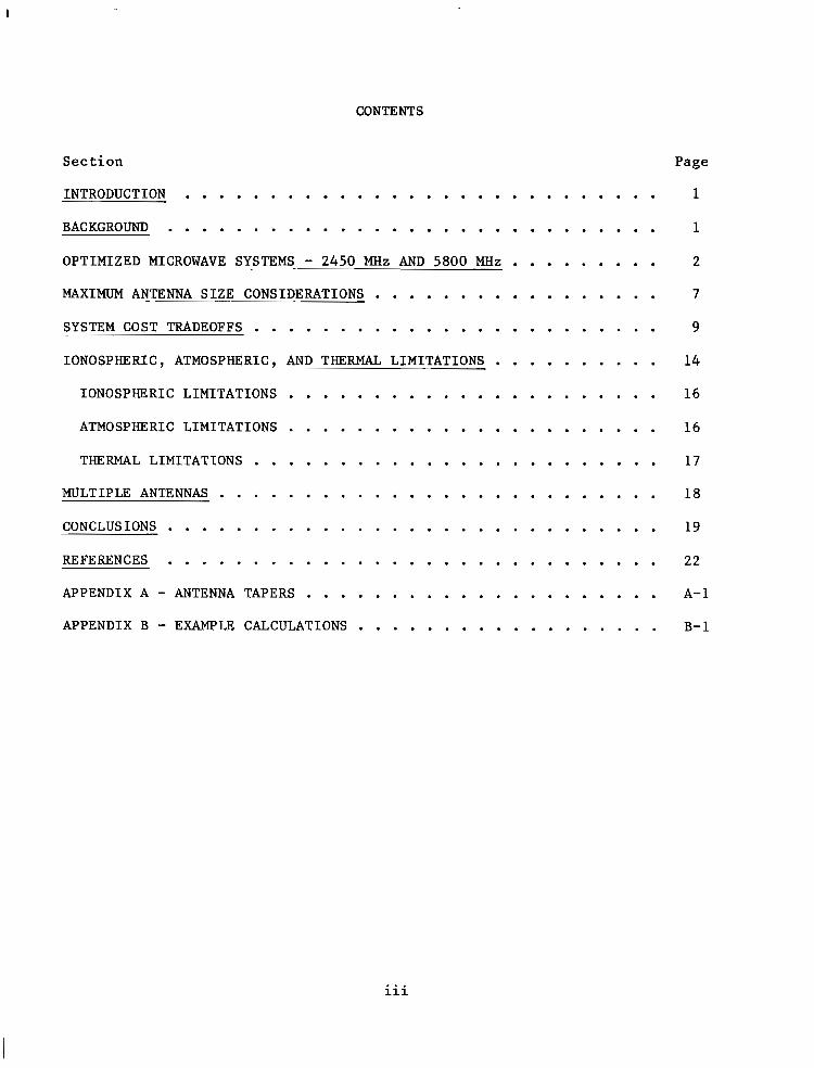
'D-GR - - 'D-ARRAY rl - 10 -dB/20 1'
A2R2 L 0.115dB J
where
'D-GR
'D-ARRAY
= peak power density at rectenna boresight
= peak power density at center of transmitting antenna
AT = transmitting antenna area
x = power beam wavelength (0.1225 m)
R = nominal range from satellite to rectenna ( 3 6 000 km)
dB = amount of dB taper for Gaussian antenna illumination (10)
'TRANS = total power radiated from transmitting antenna
For a 2.45 GHz operating frequency, two operating constraints were considered:
1. Retaining the 23 mW/cm2 ionospheric limit by reducing transmitted power as the size of the satellite antenna increased.
2. Allowing the ionospheric power density limit to increase by retaining the same transmitted power as the size of the antenna increased,
The microwave system characteristics for 2.45 GHz operation may be summarized as shown in table 1.
4

TABLE 1.- MICROWAVE SYSTEM CHARACTERISTICS AT 2.45 GHz
C h a r a c t e r i s t i c Ionospheric l i m i t No ionospheric of 23 mW/cm2 1 i m i t
Transmi t t ing an tenna diameter, km . . . . . . . .
Transmitted microwave power, GW . . . . . . . . . .
Power d e n s i t y i n i o n o - sphere, mW/ cm2 . . . . . . .
Output DC power from rectenna, GW . . . . . . . .
Rectenna diameter to cap- t u r e 88% of energy, km . . .
R e c t e n n a a r e a r e l a t i v e t o r e fe rence . . . . . . . . . .
. .
1 1.36 1.53 2 1.36 1.53 2
6.5 3.53 2.78 1.64 6.5 6.5 6.5
23 23 23 23 42 54 91
5 2.72 2.14 1.2 5 5.05 5.05
10 7.6 6.8 5 7.6 6.8 5
1.0 0.56 0.46 0.25 0.56 0.46 0.25
The thermal l i m i t of 23 kW/m2 i s not a c o n s t r a i n t f o r t h e l a r g e r a n t e n n a / sma l l e r r ec t enna sys t ems ope ra t ing a t 2.45 GHz. The ionospheric l i m i t i s the c r i t i c a l p a r a m e t e r i n s y s t e m s i z i n g f o r 2.45 GHz.
F o r o p e r a t i o n i n t h e 5.8 GHz IMS frequency band, a d i f f e r e n t set of con- s t r a i n t s must be considered. Since the gain of an antenna i s p r o p o r t i o n a l t o the frequency squared, antennas smaller than 1 km in diameter can be used with r ec t ennas smaller than the 10 km diameter re fe rence rec tennas . The antenna the rma l l imi t a t ion i s the c r i t i ca l pa rame te r fo r sys t em s i z ing a t 5.8 GHz. The ionospheric l i m i t of 23 mW/cm2 i s no longer a f ac to r because t h i s t h re sh - o l d i s a l so p ropor t iona l to f requency squared . That i s , the adjusted iono- s p h e r i c l i m i t fo r 5 .8 GHz i s
2 5 ' 8 0 = 23 [5.6] = 129 mW/cm 2 - -
'D-5.8 GHz 'D-2.45 GHz [GI
Since the 5.8 GHz antenna w i l l be smaller, o r a t least no l a r g e r , t h a n 1 km in d i ame te r , t he ad jus t ed i onosphe r i c l i m i t of 129 mW/cm2 w i l l not be exceeded . O the r f ac to r s i n f luenc ing sys t em s i z ing i nc lude l ower e f f i c i enc ie s
5

i n s e v e r a l of the microwave subsystems operating a t the higher 5.8 GHz f r e - quency. The o p e r a t i n g c o n s t r a i n t s a t 5.8 GHz are
1. Reta in ing the 23 kW/m2 antenna thermal l i m i t by reducing t ransmi t ted power as t h e s i z e of t h e s a t e l l i t e antenna decreases .
2. Allowing the antenna thermal l i m i t t o i n c r e a s e somewhat as the an tenna s ize decreases by r edes ign ing t he t he rma l r ad ia t ion sys t em.
3. Reducing subsystem efficiencies as follows:
80-percent , ra ther than 85-percent , DC-RF k lys t ron convers ion e f f i c i e n c y
97-percent , ra ther than 98-percent , eff ic iency for normal a tmospheric t ransmission
87-percent9 ra ther than 89-percent average RF-DC conversion e f f i c i e n c y i n t h e ground rectenna
The microwave system c h a r a c t e r i s t i c s f o r 5 . 8 GHz o p e r a t i o n may be summarized as shown i n t a b l e 2.
TABLE 2.- MICROWAVE SYSTEM CHARACTERISTICS AT 5.8 GHz
Charac te r i s t i c P re sen t t he rma l l i m i t of 23 kW/m2
Transmit t ing antenna diameter, km . . . . . . . . 0.75 0.5
Transmitted microwave power, GW . . . . . . . . . . 2.84 1.68
Power d e n s i t y i n i o n o s p h e r e , mw/ cm2 . . . . . . . . . . . 30 7.87
Output DC power from rectenna, GW . . . . . . . . 2 1.17
Rectenna diameter to capture 88% of t ransmit energy, km . . . . . . . . . 5.8 8.75
Rectenna area r e l a t i v e t o r e fe rence . . . . . . . . . . 0.336 0.765
Thermal 1 i m i t with improved
design
0.75 1
3.78 6.5
40 122
2.72 4.8
5.8 4.3
0.336 0.185
~~ ~
1.5
2.88
129
2.12
2.8
0.078
6

The candidate configurations have two thermal limits; i.e., the present 23 kW/m2 limit and that of an improved design, which will be discussed later.
MAXIMUM ANTENNA SIZE CONSIDERATIONS
The relative antenna and rectenna sizes for 2.45 GHz and 5.8 GHz opera- tion are shown in figure 2 . Let us now consider the mechanical and elec- tronic constraints on the maximum size for the satellite antenna as a func- tion of frequency.
One limitation on antenna size is the phase control system. An active retrodirective phase control technique is used to point and focus the down- link power beam. In the reference system, a pilot beam signal is transmitted from the ground to the satellite, where it is received and processed at each of the 101 000 power modules (tubes). A phase reference is distributed throughout the antenna to each of the power modules via a Master Slave Re- turnable Timing System (MSRTS) developed by the LinCom Corporation (ref. 2 ) .
If the antenna is enlarged, additional power modules are needed. The power output from each tube would be reduced, but the number would increase even if the overall transmitted power were lower. The reason is that the an- tenna mechanical pointing requirement for the attitude control system is de- termined by grating lobe levels which are dependent on the area of the antenna driven by one tube. Thus, given as an average antenna area associated with one tube as constrained by the antenna attitude control system, a larger an- tenna requires more power modules.
If the antenna size increases, the phase reference has to be distributed over a larger area, thereby increasing the phase error buildup. The present SPS system has a loo rms phase error budget, which consists of errors in the phase distribution system, ionosphere-induced perturbations of the uplink pilot beam signal, errors in the E@ receiver and processing electronics in each power module, etc. Larger antennas must still adhere to the 10' phase error budget in order to achieve the expected transmission efficiencies. Rectenna collection efficiencies for a 1.5 km diameter antenna with varying amounts of phase error are shown in figure 3 . The data indicate that an in- crease in phase error could easily negate the advantage of a larger antenna; i.e., a smaller rectenna.
Operating at the 5.8 GHz frequency imposes a further constraint on the phase reference distribution system within the antenna. This reference sig- nal is distributed at an intermediate frequency and is then multiplied up to the power frequency, either 2.45 GHz or 5 . 8 GHz, in the RF receiver elec- tronics in order to perform the phase conjugation of the uplink pilot signal. Because of this multiplication process, the allowable phase error within the reference distribution system is inversely proportional to the output fre- quency. Thus, operating at 5.8 GHz requires an improvement (reduction) of 5.812.45 or 2.37 in the phase distribution system error. A smaller antenna at 5.8 GHz would probably help the phase control system achieve the required performance. In summary, when considering the present reference system phase
7

e e
1 00
80
60
40
20
0
Transmitting antenna diameter (km) Figure 2.- Antenna and rectenna sizing summary.
- 88% collection ...*...............
" 0" rms phase error 10" rms phase error 20" rms phase error
- .....
Conditions: 1.53 km antenna diameter (7 = 2% failures, 0.1 dB amplitude error +
2 3 4 5 6 7 8 Rectenna diameter (km)
3.- Rectenna collection efficiency for various phase error budgets.
8

I
c o n t r o l and a t t i t u d e control requirements , reasonable antenna s izes might be a 1.5-km diameter a t 2.45 GHz and a 0.75-km diameter a t 5.8 GHz.
SYSTEM COST TWDEOFFS
A d e t a i l e d a n a l y s i s of subsystem costs and masses f o r t h e r e f e r e n c e 5 GW s o l a r power s a t e l l i t e w i t h s i l i c o n s o l a r c e l l s i s g i v e n i n r e f e r e n c e 3. These values are used as a b a s e l i n e f o r computing c o s t s f o r t h e d i f f e r e n t a n t e n n a / rec tenna conf igura t ions . S ince the purpose of t h i s r e p o r t i s to de te rmine the r e l a t i v e o r d i f f e r e n t i a l c o s t s f o r t h e v a r i o u s c o n S i g u r a t i o n s , any f u t u r e changes in t he abso lu t e cos t s fo r t he r e f e rence sys t em shou ld no t have a g r e a t impact on the conclusions s ta ted herein.
The p r inc ipa l e l emen t s i n t he SPS r e c u r r i n g c o s t s are
1. S a t e l l i t e h a r d w a r e
2. Transpor ta t ion ( space and ground)
3 . Space construction and support
4. Rect enna
5 . Program management and i n t e g r a t i o n
6 . Cost a l lowance for mass growth
Some general cost ing assumptions include
1.
2.
3 .
4.
5.
6.
7.
30-year opera t ing l i fe t ime
0 . 9 2 p l a n t f a c t o r f o r 2.45 GHz opera t ion
0 . 9 0 p l a n t f a c t o r f o r 5.8 GHz o p e r a t i o n
15-percent ra te of r e tu rn on i nves tmen t cap i t a l
22-percent mass g r o w t h f a c t o r t o c o v e r p o t e n t i a l r i s k s i n s o l a r a r r a y and microwave system performance estimates
17-percent of n e t SPS ha rdware cos t f ac to r t o accoun t fo r mass growth
10 GW pe r yea r add i t iona l power gene ra t ion capac i ty
9
I

The t o t a l mass and c o s t f o r t h e r e f e r e n c e SPS system are 59 984 m e t r i c tons and $12 432 m i l l i o n . The cost and mass s t a t e m e n t s f o r t h e i n d i v i d u a l s a t e l l i t e subsystem are d iv ided i n to t he fo l lowing ca t egor i e s :
1. Power c o l l e c t i o n : s t r u c t u r e , s o l a r ce l l s , power d i s t r i b u t i o n , and maintenance
2. R o t a r y j o i n t
3. Power t r ansmiss ion : s t ruc tu re , k lys t rons and thermal control , wave- g u i d e s , s u b a r r a y s t r u c t u r e , power d i s t r ibu t ion ( conduc to r s , swi t ch - gea r s , DC-DC conver te rs , thermal cont ro l ) , energy s torage , phase control, maintenance systems, and antenna mechanical point ing
4. Information management and a t t i tude cont ro l : hardware and propel lan t
5. Communications
6 . T r a n s p o r t a t i o n : e l e c t r i c o r b i t t r a n s f e r v e h i c l e (EOTV), personnel launch vehic le (PLV), p e r s o n n e l o r b i t t r a n s f e r v e h i c l e (POTV), and heavy l i f t l aunch vehic le (HLLV)
7 . Cons t ruc t ion opera t ions : low Ear th o rb i t (LEO) and geosynchronous o r b i t (GEO)
The c o s t and mass from each of these subsystems w i l l va ry acco rd ing t o t o t a l power, an tenna s ize , f requency , e tc . of the candidate antenna/rectenna sys t ems . S ince t he ca l cu la t ions are qu i t e l eng thy , on ly t he end r e s u l t s f o r 2.45 GHz and 5.8 GHz o p e r a t i o n are shown i n t a b l e s 3 and 4. The d e t a i l s are g iven in appendix B, t oge the r w i th a complete sample calculat ion for one con- f i g u r a t i o n . I n t a b l e 3 (2.45 GHz), the microwave system has been sized to conform with the 23 mW/cm2 ionospheric l i m i t f o r t h e f i r s t f o u r a n t e n n a / r ec t enna conf igu ra t ions . Th i s i onosphe r i c cons t r a in t has been removed f o r t h e l a s t t h r e e c o n f i g u r a t i o n s , r e s u l t i n g i n a maximum of 91 mW/cm2 f o r t h e 5 GW, 2 km diameter antenna system.
The e l e c t r i c i t y c o s t s i n m i l l s per kwh and t h e d i f f e r e n t i a l c o s t i n c r e a s e as compared t o t h e 5 GW, 1-km antenna re ference sys tem a re shown i n f i g u r e 4 f o r 2.45 GHz ope ra t ion . The top curve , cons t ra ined to an ionospher ic l i m i t of 23 mW/cm2, shows a s i g n i f i c a n t i n c r e a s e i n e l e c t r i c i t y c o s t as the antenna s i z e i n c r e a s e s . Microwave power d e n s i t y i n t h e i o n o s p h e r e i s d i r ec t ly p ropor - t i o n a l t o t r a n s m i t t i n g a n t e n n a area and t o t a l t r a n s m i t t e d power; t h e r e f o r e , i f the antenna area i s doubled, the power must be reduced by one-half i n o r d e r t o ma in ta in t he same power dens i ty . The e l e c t r i c i t y c o s t r a t e s ( m i l l s / k W h ) a r e determined by t h e t o t a l s a t e l l i t e c o s t s d i v i d e d by the de l ive red power. A s t h e c o s t summary i n t a b l e 3 shows, the total s a t e l l i t e c o s t s d e c r e a s e a t a much s lower ra te than does the del ivered power as t h e a n t e n n a s i z e i n c r e a s e s . The cost d isadvantage with larger antennas i s removed i f t h e t o t a l t r a n s m i t t e d power remains constant as the antenna s ize changes. However, t h e i o n o s p h e r i c power dens i ty i nc reases acco rd ing ly .
10

TABLE 3.- SPS SLTMMARY COSTS FOR 2.45 GHz OPERATION
( a ) P h y s i c a l p a r a m e t e r s
23 mWlcm2 i o n o s p h e r i c I n c r e a s e d i o n o s o h e r i c S p e c i f i c a t i o n 1 i m i t l i m i t
~ -__
1.53 2 1.36 1 .53 2
2 .78 1.64 6 . 5 6 . 5 6 .5
A n t e n n a d i a m e t e r , km . . . . . . . S a t e l l i t e power o u t p u t , GW . . . . Power d e n s i t y a t r e c t e n n a ,
mw/ cm2 . . . . . . . . . . . . . R e c t e n n a d i a m e t e r , km . . . . . . Power d e l i v e r e d , GW . . . . . . .
1
6 .5
23
10
5
1.36
3.53
23
7.6
2.7
23 23 42 54 91
6.8 5 7 .6 6 .8 5
2 .1 1.26 5 5.05 5 .05 . ~ . . . ""
Cos t c a t e g o r y I n c r e a s e d i o n o s p h e r i c 1 i m i t
23 mW/cm2 i o n o s p h e r i c l i m i t
SPS h a r d w a r e , m i l l i o n d o l l a r s . . . . . . . . . . . .
L e s s a m o r t i z a t i o n of i n v e s t m e n t , m i l l i o n d o l l a r s . . . . . . . . . . . . .
T o t a l , m i l l i o n d o l l a r s . . . . . M i s s i o n c o n t r o l , m i l l i o n
d o l l a r s . . . . . . . . . . . T r a n s p o r t a t i o n , m i l l i o n
d o l l a r s . . . . . . . . . . . . C o n s t r u c t i o n o p e r a t i o n s ,
m i l l i o n d o l l a r s . . . . . . . . R e c t e n n a , m i l l i o n d o l l a r s . . . . Program management and
i n t e g r a t i o n , m i l l i o n d o l l a r s . . . . . . . . . . . .
C o s t a l l o w a n c e f o r m a s s g r o w t h , m i l l i o n d o l l a r s . . . .
T o t a l , m i l l i o n d o l l a r s . . . . . . Mills p e r kwh . . . . . . . . . . C e n t s p e r MJ . . . . . . . . . . . % i n c r e a s e i n e l e c t r i c i t y
c o s t s c o m p a r e d t o c o s t o f 1 . 3 ~ 1 M . J ( 4 7 m i l l s / k W h ) f o r t h e r e f e r e n c e SPS s y s t e m . . . .
4946 4072 4120 5069 5898 6455 8112
4 7 3
4473
257
381 5
202 119 473 473 4 7 3
3918 4950 5425 5982 7639
1 0 1 0 10 10 10
2721 31 86 3639 3918 4849
1170 1615 1233 1395 1933
1293 835 1852 1646 1283
10 10
31 20 2700
96 1
2578
1066
1561
495 407 41 2 50 7 5 90 64 5 81 1
760
12 432
47
1.3
64 9
10 243
71.6
2.0
666 84 1 922 1017 1299
1 0 1 9 0 11 944 13 671 14 613 17 824
90.6 180 .1 52 55 67.1
2.5 5 . 0 1 .4 1 .5 1 .9
52.4 92.7 283 10.6 17 42 .7
11

TABLE 4 . - SPS SUMMARY COSTS FOR 5 . 8 GHz OPERATION
( a ) P h y s i c a l p a r a m e t e r s
S p e c i f i c a t i o n
A n t e n n a d i a m e t e r , km . . . . . . . S a t e l l i t e power o u t p u t , GW . . . . Power d e n s i t y a t r e c t e n n a ,
mW/ cm2 . . . . . . . . . . . . . R e c t e n n a d i a m e t e r , km . . . . . . Power d e l i v e r e d , GW . . . . . . .
P r e s e n t t h e r m a l d e s i g n
0 . 7 5
2 . 8 4
30
5 .a 2
.
C o s t c a t e g o r y
-~ .
SPS h a r d w a r e , m i l l i o n d o l l a r s . . . . . . . . .
L e s s a m o r t i z a t i o n of inves tment , m i 11 i o n d o l l a r s . . . . . . . . .
T o t a l , m i l l i o n d o l l a r s . . . M i s s i o n c o n t r o l , m i l l i o n
d o l l a r s . . . . . . . . . T r a n s p o r t a t i o n , m i l l i o n
d o l l a r s . . . . . . . . . C o n s t r u c t i o n o p e r a t i o n s ,
m i l l i o n d o l l a r s . . . . . R e c t e n n a , m i l l i o n d o l l a r s . Program management and
i n t e g r a t i o n , m i l l i o n d o l l a r s . . . . . . . . .
Cos t a l l owance f o r mass g r o w t h , m i l l i o n d o l l a r s .
T o t a l , m i l l i o n d o l l a r s . . . Mills p e r kwh . . . . . . . C e n t s p e r M J . . . . . . . . % i n c r e a s e in e l e c t r i c i t y
c o s t s c o m p a r e d t o c o s t of 1.3clM.l ( 4 7 m i l l s / k W h ) f o r t h e r e f e r e n c e SPS sys t em a t 2.45 GHz . . . . . . .
( b ) C o s t s
.~
. . .
. . .
. . .
. . .
. . .
. . .
. . .
. . .
. . .
. . .
. . .
. . .
. . .
Improved thermal d e s i g n
0 .5 0 .75 1 .0 1.5
1 . 6 8 3 . 7 8 6 . 5 2.88
7.87 4 0 1 2 2 1 2 9
8 . 7 5 5 .a 4 . 3 2 . 8
1 .17 2 .72 4.8 2 .12
Present Improved thermal t h e r m a l d e s i g n d e s i g n
...
1452
122
1330
10
12aa
444
4925
145
226
a368
138
3.8
193
12
275 473 209 206
2763 4893 4568 22aa
10 1 0 10 1 0
2070 3120 2720 1794
734 1057 1270 663
2672 2003 1063 2578
303 536 477 249
4 7 0 a3 2 777 389
9022 12 451 10 aa5 7969
6 4 5 0 . 3 9 9 7 6 . 1
I . a 1 . 4 2 . 7 2 . 1
36 7 111 62

5 .O
4.4
3.9
2 3.3 \ t4 - 2.8 cn cn 0
)r
0
0
+
0 2.2 + .- .= 1.7
2 1.3 w 1.1
+
1 80
160
140 3 > 120 x
- - .- E - 100 cn cn 0 .c,
0 80
.- 0 h 60
280 +- cn cn
240
23mW/cm2 ionospheric / limit .
I .- C
. . .-*' Increasing ..-* ionospheric
Reference .* .*
120 $ a, cu
1 .O 1.25 1.5 1.75 2.0 Transmitting antenna diameter (km)
80 '0 C .- +
40 2 a, a 0
Figure 4 . - Electricity costs for 2.45 GHz systems.
13

The 5.8 GHz sys t ems desc r ibed i n t ab l e 4 have t he rma l l imi t a t ions i n t h e t r a n s m i t t i n g a n t e n n a r a t h e r t h a n i o n o s p h e r i c l i m i t a t i o n s as t h e dominant c o n s t r a i n t . The 5.8 GHz systems are i n h e r e n t l y smaller (an tenna , t ransmi t ted power, and r ec t enna ) as compared t o t h e 2.45 GHz conf igu ra t ions as a r e s u l t of the increased antenna gain a t h ighe r f r equenc ie s .
The e l e c t r i c i t y c o s t s f o r t h e 5 . 8 GHz systems are compared t o t h e r e f e r - ence 2.45 GHz system i n f i g u r e 5. The d a t a i n d i c a t e t h a t a s ign i f i can t r educ - t ion in cos ts can be ach ieved wi th a modest improvement i n the rma l r ad ia to r d e s i g n . S i n c e t h e i n c r e a s e i n d i f f e r e n t i a l c o s t i s reduced from 64 pe rcen t t o 36 percent for the 0 .75 km diameter antenna by using a new thermal radia- t o r c o n f i g u r a t i o n , improvements in thermal design are considered mandatory. D e t a i l s of t he t he rma l des ign e s t ima tes a r e g iven i n a l a t e r s e c t i o n .
I n summar iz ing the cos t ing resu l t s and the microwave system tradeoffs, s eve ra l op t ions shou ld be cons ide red fu r the r :
2.45 GHz
' I n c r e a s e ionospheric l i m i t -- 1.53-km antenna; 6.8-km rec t enna t o 54 mW/cm2 with 5 GW g r i d power; d i f f e r e n t i a l
c o s t i n c r e a s e i s 1 7 p e r c e n t ( t o 1.5c/MJ (55 mills/kWh))
Re ta in 23 mW/cm2 -- 1.36-km antenna; 7.6-km rec t enna as ionospheric with 2.7 GW g r i d power; d i f f e r e n t i a l 1 i m i t c o s t i n c r e a s e i s 50.2 percent ( to
2.Oc/M.J (70.6 mills/kWh))
5.8 GHz Increase an tenna -- 0.75-km antenna; 5.8-km rec t enna thermal l i m i t by with 2.72 GW g r i d power; d i f f e r e n t i a l 33 percent c o s t i n c r e a s e i s 36 p e r c e n t ( t o
1.8c/MJ (64 mills/kWh))
The microwave r a d i a t i o n p a t t e r n s f o r t h e 1.53-km antenna opera t ing a t 2.45 GHz and the 0.75-km a n t e n n a o p e r a t i n g a t 5.8 GHz a r e compared i n f i g u r e 6 wi th the l-km antenna, 5 GW r e f e r e n c e SPS system.
IONOSPHERIC , ATMOSPHERIC,- AND THERMAL . . . LIMITATIONS . .
The r e l a t i v e e l e c t r i c i t y c o s t s f rom the var ious antenna/rectenna configu- r a t i o n s are heavily dependent upon the ionospheric, atmospheric, and thermal c o n s t r a i n t s imposed on the microwave systems. The v a l i d i t y of t hese con- s t r a i n t s i s under review and may be r ev i sed pend ing t he r e su l t s of a number of s t u d i e s .
14

3.9
3.3
2.8 I \ e v
* 2.2 cn cn 0 0
c. >r '0 .- 1 . 7 Y L
$ 1 . 3 1.1
-
100;
L
10
h
N
E
1 ool
80
60
40
Transmitting antenna diameter (km)
Figure 5.- E l e c t r i c i t y c o s t s for 5.8 GHz systems.
1.53-km antenna, 2.45 GHz, rectenna output power= 5.05 GW
antenna, 5.8 GHz, rectenna output 2.72 GW
- 1 -km antenna, 2.45 GHz, rectenna output power=5 GW
-- Power density level at edge of rectenna
3 Radius from rectenna boresight (km)
n 1
ool Costs using present antenna thermal limit
80
Reference
I o .75 1 .o 1.25 1.5
Costs using present antenna thermal limit
Reference system costs P- I o
.5 .75 1 .o 1.25 1.5
a
1 5
Figure 6 . - Antenna pat terns for t h r e e SPS conf igu ra t ions .
15

IONOSPHERIC LIMITATIONS
Res i s t ive (ohmic ) hea t ing e f f ec t s by t h e power beam may produce nonlin- ear i n s t a b i l i t i e s s u c h as enhanced e lec t ron hea t ing in the lower ionosphere (D and E r eg ions ) and t he rma l s e l f - focus ing e f f ec t s i n t he uppe r i onosphe re (F region) . The Department of Energy (DOE) has recent ly sponsored a number of ionospheric s tudies which include ( 1 ) t h e o r e t i c a l and experimental anal- yses of t h e e f f e c t s of underdense heating upon ionospheric physics, performed i n p a r t a t the Arec ibb , Puer to Rico , observa tory ; (2) exper imenta l s tud ies by the Ins t i tu te for Te lecommunica t ion Sc iences ( ITS) in to hea ted ionospher ic e f f e c t s upon low frequency connnunication and navigation systems (loran, OMEGA, WWV, and AM b roadcas t ing s t a t ions ) . Th i s ITS work i s being performed under the d i r ec t ion o f Cha r l e s Rush u s i n g t h e P l a t t e v i l l e , C o l o r a d o , h e a t i n g f a c i l i t y .
The r e s u l t s of t he t e s t s pe r fo rmed t o da t e a t Arecibo and P l a t t e v i l l e show no ev idence to suppor t 23 mW/cm2 as an upper l i m i t . The e l e c t r o n t e m - pera ture increases due to underdense hea t ing are a f a c t o r of 2 o r 3 , r a the r than the o rder of magn i tude p red ic t ed i n t he ea r ly ana lyses ( r e f . 4 ) . The theory i s now be ing r ev i sed and i n i t i a l r e s u l t s p r e d i c t a l / f 3 h e a t i n g r a t h e r t h a n l / f 2 . The l / f 3 h e a t i n g would i n c r e a s e t h e power dens i ty l i m i t . I n addi- t i o n , t h e r e are no i n d i c a t i o n s of i r r e g u l a r i t i e s b e i n g formed i n t h e l o w e r ionosphere during underdense heat ing. Effects produced by s imulated SPS h e a t i n g a r e many times less than na tu ra l i onosphe r i c d i s tu rbances c r ea t ed by s o l a r f l a r e s ( p r i v a t e communication from C. Rush, Dec. 1979).
An ionosphere power d e n s i t y l e v e l of 50-60 mW/cm2 may be a reasonable l i m i t and would accommodate the 54 mW/cm2 level produced by the 1.5-km anten- na, 5 GW s a t e l l i t e system. More ionosphe r i c s tud ie s w i th upgraded f ac i l i t i e s a t Arec ibo and P la t tev i l le to p roduce 50-60 mW/cm2 equ iva len t hea t ing l eve l s in the upper ionosphere (F r e g i o n ) a r e n e e d e d t o v e r i f y t h e h i g h e r l imi t s .
ATMOSPHERIC LIMITATIONS
The e f f i c i e n c y b u d g e t f o r t h e 2.45 GHz re fe rence conf igu ra t ion has 98-percent transmission (2-percent loss) through the atmosphere. This sig- n a l a t t e n u a t i o n i s p r i m a r i l y d u e t o r a i n and atmospheric absorption. The 2-percent a t tenuat ion , o r 130 MW loss, r e p r e s e n t s a bad case (but not the wors t poss ib le condi t ion) for the 2 .45 GHz frequency. The 5.8 GHz frequency has approximately the same transmission eff ic iency as has the 2 .45 GHz through a nonrainy atmosphere, but the 5.8 GHz frequency i s severely degraded under ra iny condi t ions . The l o s s e s f o r two systems providing 5 GW of ground g r i d power may be summarized as follows (refs. 5 and 6):
1 6

Medium
Ionosphere
Neutral a tmosphere a t mid-United States l a t i tude (water vapor and oxygen
abso rp t ion )
Rain Heavy ( 1 5 mmlhr over 15-km path)
Cen t ra l /Eas t e rn U.S. - 9 h r / y r Southern U.S. - 3 h r / y r Western U.S. - 3 h r / y r
Moderate ( 5 mmlhr over 10-km pa th) Cen t ra l lEas t e rn U.S. - 4 5 h r / y r Southern U.S. - 85 h r / y r Western U.S. - 10 h r / y r
A t t enua t ion l o s ses
2.45 GHz 5.8 GHz
0.25 kW 1 kW
90 Mw 100 Mw
148 MW
34 Mw
1.8 GW
405 MW
Wet h a i l 2.6 GW 4.99 GW
The 2.45 GHz frequency has very minimal losses due to nonideal weather condi- t i o n s ; t h e 5.8 GHz f r e q u e n c y o p e r a t e s s a t i s f a c t o r i l y i n t h e d r y c l i m a t e s o f the southwes tern Uni ted S ta tes bu t would su f fe r ou tages i n we t t e r r eg ions .
The impact on a commercial u t i l i t y g r i d of a 5.8 GHz microwave system t h a t may have t o be shut down on an unscheduled basis because of weather ef- f e c t s i s not known. I f a 5.8 GHz microwave system i s t o b e s e r i o u s l y con- s i d e r e d a s a n a l t e r n a t i v e t o a 2.45 GHz system, then an indepth s tudy of this ques t ion i s requi red .
THERMAL LIMITATIONS
Since an tenna thermal rad ia t ion i s a m a j o r c o n s t r a i n t f o r a 5.8 GHz sys- t e m , an i nves t iga t ion i n to t he uppe r t he rma l l i m i t was undertaken. The i n i - t i a l d e s i g n f o r t h e t h e r m a l r a d i a t o r s i n t h e r e f e r e n c e SPS sys t em (g iven i n r e fe rence 7 ) was found t o be q u i t e c o n s e r v a t i v e and improvements ( i n c r e a s e s ) i n t h e amount of waste h e a t r e j e c t i o n are poss ib l e . The major improvement i s due to u s ing g raph i t e compos i t e ma te r i a l s w i th a h igh emis s iv i ty coa t ing fo r t h e r a d i a t o r , as w a s proposed several years ago by Grumman i n t h e s y s t e m de- s i g n f o r c r o s s f i e l d a m p l i f i e r s .
It i s f i r s t n e c e s s a r y t o estimate t h e RF l o s s e s and determine where they o c c u r i n a 5.8 GHz klys t ron tube . A pre l iminary estimate, as provided by
17

E. Nalos of the Boeing Company, of t he waste hea t sou rces fo r a 70 kW tube o p e r a t i n g a t 80-percent e f f ic iency i s given below:
Co l l ec to r : 9.7 kW a t 773 K (500° C)
Cavity: 4.3 kW a t 573 K (300' C)
Solenoid: 3.5 kW a t 573 K (300° C)
To ta l l o s ses 17 .5 kW
Using the Stefan-Boltzmann equat ion for heat radiat ion, wi th a f i n e f f i - c iency of 80 percent and 85 -pe rcen t e f f i c i ency fo r t he emis s iv i ty of t h e coa t ings , t he r equ i r ed r ad ia to r areas are
2.22 m2 - f o r c o l l e c t o r r a d i a t o r s a t 773 K (500' C)
.76 m2 - f o r c a v i t y a n d s o l e n o i d r a d i a t o r s a t 573 K (300' C)
.22 m2 - 7 pe rcen t add i t iona l area for mechanica l spac ings
3.2 m2 - t o t a l r a d i a t o r a r e a p e r t u b e
The waste h e a t r a d i a t e d p e r u n i t area i s 17.5 kW/3.2 m2 = 5.46 kW/m2, an inc rease of 33 percent over the re fe rence SPS design, which radiates 4.1 kW/m2. The corresponding RJ? r a d i a t e d power pe r un i t area i s 70 kW/3.2 m2 = 21.9 kW/m2. The t o t a l t r a n s m i t t e d power from a 0.75 km diameter an tenna rad ia t ing a t 5 .8 GHz with 70-kW k l y s t r o n s o p e r a t i n g a t 80-percent e f f ic iency may be c a l c u l a t e d u s i n g e q u a t i o n (2) :
where dB = amount of dB taper for Gauss ian an tenna i l lumina t ion (10) .
Th i s t r ansmi t t ed power of 3780 Mw has been used i n t a b l e s 2 and 4 t o c a l - culate system performance and e l ec t r i c i ty cos t s . Cor re spond ing t r ansmi t t ed power values are ca l cu la t ed fo r t he o the r an t enna / r ec t enna conf igu ra t ions us ing t he same technique. It appears that an increased thermal l i m i t i s fea- s i b l e f o r t h e 5 . 8 GHz systems (and a lso for the 2 .45 GHz sys tems) . In gen- e ra l , ope ra t ing a t the higher frequency makes the thermal radiation problem more d i f f i c u l t s i n c e t h e t u b e s are p h y s i c a l l y smaller and present a l a r g e r heat load.
MULTIPLE ANTENNAS
The p resen t SPS scenar io has 60 s a t e l l i t e s s e p a r a t e d 1' (700 km) i n geo- synchronous o rb i t , each de l iver ing 5 GW of r ec t enna DC g r i d power. Because
18

of inc reased demands for geosynchronous s lots by o t h e r u s e r s , i t may become necessary to reduce the number of SPS sa t e l l i t e s . Mult iple antennas on one SPS s a t e l l i t e are recommended. It has been shown t h a t SPS antennas can oper- a t e in c lose p rox imi ty w i th neg l ig ib l e i n t e r f e rence f rom each 0 the r . l An example of a mul t ip le an tenna sys tem would be a 5 km by 20 km s o l a r a r r a y ( t w i c e t h e s i z e of the p resent so la r a r ray for one an tenna) feed ing two 5 GW antennas, one a t each end. It may be advantageous t o have four or more anten- nas on a s i n g l e s a t e l l i t e e s p e c i a l l y i f a l a rge r an t enna / sma l Ie r r ec t enna con- f i g u r a t i o n o r a higher frequency (5.8 GHz) system i s chosen. The r e l a t i v e s i z e s f o r a number of an tenna/ rec tenna conf igura t ions are shown i n f i g u r e 7 .
CONCLUSIONS
The s a t e l l i t e and a s s o c i a t e d microwave system have been reoptimized with l a rge r an t ennas ( a t 2.45 GHz), reduced output power and smaller rectennas. Four cons t r a in t s were considered: (1) the 23 mW/cml ionosphe r i c l i m i t , (2 ) a higher (54 mW/cm2) ionosphe r i c l i m i t , ( 3 ) the 23 kW/m2 thermal l i m i t i n t h e a n t e n n a , and (4) an improved thermal design for the 5.8 GHz systems allowing 33 percent addi t iona l was te hea t . The d i f f e r e n t i a l c o s t s i n e l e c - t r i c i t y f o r s e v e n a n t e n n a / r e c t e n n a c o n f i g u r a t i o n s o p e r a t i n g a t 2 . 4 5 GHz and f i v e s a t e l l i t e s y s t e m s o p e r a t i n g a t 5.8 GHz have been calculated. The con- c l u s i o n s a r e
1. Larger antenna/smaIler rectenna configurat ions are economical ly fea- s i b l e u n d e r c e r t a i n c o n d i t i o n s .
2. Transmit t ing antenna diameters should probably be l i m i t e d t o 1-1.5 km f o r 2.45 GHz ope ra t ion and 0.75-1.0 km for 5 .8 GHz because of phase cont ro l , c o n s t r u c t i o n c o s t s , and a t t i t u d e c o n t r o l .
1G. D. Arndt and J. W. Seyl: RF In t e r f e rence /Orb i t a l Spac ing Ana lys i s f o r S o l a r Power Sa te l l i t es . Lyndon B. Johnson Space Center (Houston, Tex.), t o be published.
19

Single antenna configurations
5 km 2.45 GHz 5.8 GHz
Relative satellite size
nlo km
0 Transmitting 1 km 1.36 km 1.53 km antenna diameter
Relative rectenna size 0 0 0
l O x l 3 k m 7.6x9.9km 6.8x8.8km Ground power 5 GW 2.7 GW 5.05 GW output
Multiple antenna configurations
Two - 5 GW, 1 km dia. systems a t 2.45 GHz
0
Four - 5.05 GW, 1,53 km dia. systems a t 2.45 GHz
0.75 km 1 km 1.5 km
1 l o x 13 km I 6.8 x 8.8 km
5 . 8 ~ 7.5 km 4.3 x 5.6 km 2.8 x 3.6 km
2.72 GW 4.78 GW 2.12 GW
Four - 272 GW, .75 km dia. systems a t 5.8 GHz
I 15.8 x 7.5 km
Figure 7.- Relative sizes for several antenna/rectenna configurations.
20
I

3. Two 2.45 GHz configurations are selected, dependent upon the iono- spheric power density limit.
23 mW/cm2 54 mW/cm2 1 imi t 1 imi t
Antenna diameter, km . . . . . . . . . . 1.36 1.53 Rectenna DC grid power, GW . . . . . . . 2.76 5.05 Rectenna diameter, km . . . . . . . . . 7.6 6.8 Relative rectenna area, % . . . . . . . 56 46 Electricity cost increase, % . . . . . . 50.2 17 Electricity cost, mills/kWh . . . . . . 70.6 55 Electricity cost, c/MJ . . . . . . . . . 2.0 1.5
Note: The rectenna areas and electricity costs are in comparison to those for the reference SPS system.
4. The present ionospheric limit of 23 mW/cm2 is too low and should be raised after the ionospheric heating tests and studies are completed. Be- cause of SPS cost considerations, it is very important to ascertain the true upper limit .
5. The 5.8 GHz configurations are constrained by antenna thermal limita- tions rather than ionospheric limits. A reasonable configuration based on a 33-percent improvement in waste heat rejection is
Antenna diameter, km . . . . . . . . . . 0.75
Rectenna grid, km . . . . . . . . . . . 5.8 Relative rectenna area, % . . . . . . . 33
Rectenna DC grid power, GW . . . . . . . 2.72
Electricity cost increase, % . . . . . . 36 Electricity cost, mills/kWh . . . . . . 64 Electricity cost, c/MJ . . . . . . . . . 1.8
6. The impact on commercial utility grids of a 5.8 GHz system that has to be shut down on an unscheduled basis due to localized weather conditions should be investigated.
7. Multiple (two to four) antennas on a single solar satellite are def- initely recommended regardless of the particular antenna/rectenna configura- tion chosen. This is a means of maintaining the same amount of power supplied to the ground while reducing the number of geosynchronous slots (spacings) required for the satellites.
Lyndon B. Johnson Space Center National Aeronautics and Space Administration
Houston, Texas, December 5, 1980 986-15-89-00-72
21

REFERENCES
1 . S a t e l l i t e Power System: Concept Development and Evaluation Program, Ref- erence System Report. NASA TM-79762, 1979.
2. Lindsey, W. C.: A S o l a r Power Sa te l l i t e T ransmiss ion Sys t em Inco rpora t ing Automatic Beamforming, Steer ing and Phase Control . Rep. TR-7806-0977, LinCom Corp. (Contract NAS 9-152371, June 1978.
3. Solar Power S a t e l l i t e System Defini t ion Study - Phase 11. Volume I1 - Reference System Description. Boeing Aerospace Co. (Cont rac t NAS 9-15636). NASA CR-160443, 1979.
4. Duncan, L e w i s M.; and Gordon, William E. : Ionospher ic Power B e a m S tud ie s . Paper presented a t SPS Workshop on Microwave Power Transmission and Reception (Houston, Tex.), Jan. 15-18, 1980.
5. Gordon, William E . ; and Duncan, L e w i s M.: Ionosphere/Microwave Beam In- t e r ac t ion S tudy , F ina l Repor t . R ice Un ive r s i ty (Con t rac t NAS 9-15212). NASA CR-151821, 1978.
6 . Park, K. Y. : At tenuat ion of S-Band, X-Band, and Ku-Band S i g n a l s i n a One-way and Two-way Ear th- to-Sa te l l i t e L ink . Rep. ASAO-PR20079-9, Magnavox Government and I n d u s t r i a l E l e c t r o n i c s Co., Feb. 1979.
7 . So lar Power S a t e l l i t e System Defini t ion Study - P a r t 11. Volume I V - Microwave Power Transmission Systems. Boeing Aerospace Co. (Cont rac t NAS 9-15196). NASA (33-151668, 1977.
22

APPENDIX A
ANTENNA TAPERS
The antenna illumination taper for the reference SPS system was optimized to provide maximum rectenna collection efficiency while minimizing sidelobe levels. Previous simulation results for a 1-km antenna indicated that a 10-dB Gaussian taper maximized the rectenna collection efficiency in the 85-90 per- cent range while satisfying the antenna thermal constraints. These data, taken for an antenna operating with the specified error parameters (i.e., (5 = loo phase error, kO.1 dB amplitude error, and 2 percent tube failures) yield an 88-percent collection efficiency over approximately a 10 km diameter rectenna. This appendix addresses the question of whether other tapers would be more efficient with larger antennas.
The results are given in figure A-1 for a 1-km antenna operating with no errors and a 2-km antenna transmitting with the specified error parameters. As the amount of taper increases, the main beam peak intensity decreases and the beam width increases. There is more power in the main beam and less power in the near sidelobes. This condition increases the rectenna collection ef- ficiency. Both systems achieve good performance, with rectenna collection efficiency in the 85-90 percent range using a 10-dB taper. All the SPS con- figurations in this report have a 10-dB taper.
A- 1

c = 0 501
15
10
”
”-
””
.. - .. 0 dB 2 km, 1.26 GW,U=l O0,& 0.1 dB,
.............. + 0 a,
40 1 2 3 4 5 6 7 8 9
Rectenna radius (km) Figure A-1. - Rectenna collection efficiency VS. array taper.
A- 2

APPENDIX B
EXAMPLE CALCULATIONS
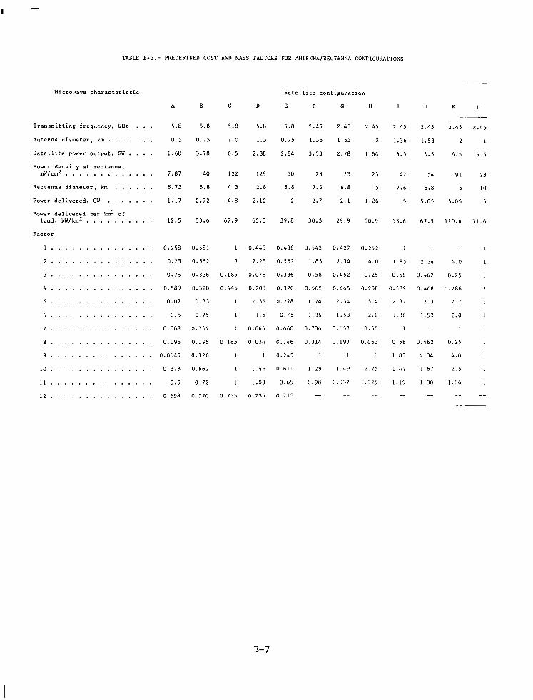
The purpose of this appendix is to review the assumptions, methods, and steps by which cost and mass were calculated for various SPS configurations. The rationale is explained in the body of the text. The Boeing-JSC reference design cost and mass numbers were used as the basis for all comparative calcu- lations in this study. Where applicable, these numbers are included as case L. Study assumptions are defined in table B-1, and cost and mass (C/M) factors are included in table B-2. The factors referred to in table B-1 are defined in table B-2. They were used to estimate new costs and masses for the various alternative configurations.
Factor values are presented in table B-3. In case A , the satellite RF power output is 1.68 GW. Factor 1 is calculated by dividing this number by 6.5 GW, as explained in table B-2. The resulting value of factor 1 is 0.258. The antenna diameter in case A is 0.5 km. Therefore, factor 2 is calculated (0 .5 )2 / (1 )2 = 0.25. The reference rectenna diameter (case L ) excluding the buffer zone is 10 km. In case A , the rectenna diameter is 8.75 km. Factor 3 is then given by (8.75)2/( 1012 = 0.76. Factor 4 is the relative land area including the buffer zone out to 0.1 mW/cmZ. For case A , major and minor di- ameters are found in table B-4 (12.9 km and 9.2 km). Factor 4 is thus calcu- lated 71 (12.9) (9.2) i 4 (158.3) = 0.589. The buffer zone area for the refer- ence configuration is given in table B-5. Before factor 5 can be calculated, the total mass of the transmitting antenna in question must be estimated. Factor 6 is required for maintenance system mass. It is determined by ex- tracting the s uare root of factor 2. In this case factor 2 was 0.25, so factor 6 is P- 0.25 = 0.5.
Factors 7, 8 , 9 , and 10 are simple calculations based on factors 1, 2, and 3 . Factor 11 is used for calculating HLLV costs as a portion of factor 13. In the reference case, 208 launches are required - 94 for solar power systems, 46 for the transmitting antenna, and 68 for other purposes. Factors 1 and 2 are used in scaling factor 11 for HLLV costs, as is shown in table B-2. Be- cause of the simplicity of factors 12-16, a detailed explanation of their cal- culation is not necessary (see table B-2) .
In table B-5, the values for reference system mass and cost are listed in the last two columns. The first two columns (case F) are derived by mul- tiplying the last two columns, respectively, by the appropriate factor value from table B-3. The mass of the power collection structure, for example, is found by multiplying 4654 X 0.543 = 2527. In this manner, values are found for all costs and masses until antenna mechanical pointing is reached. This requires the use of factor 5 , which has not been determined. To overcome this obstacle, the mass for mechanical pointing is assumed to be the same as the reference. Using this value, an interim total power transmission mass is found. Factor 5 is determined using this mass, and a new mechanical point- ing value is calculated using the factor 5 value. Then a more accurate power transmission mass is totaled.
B- 1

A s can be calculated from the first mass column in table B-5, the sub- total of all power transmission masses except that for mechanical pointing is 12 679 t. Adding 134 t to this from the Last mass column (reference case) results in 12 813 t for the interim total. The power transmission mass total for the reference case is 13 628 t. From the definition in table B-2, fac- tor 5 (for case F) turns out to be
(12 813) x (1.36)2/(13 628)(1)2 = 1.74
This value of factor 5 is then used to determine a new value for the mechani- cal pointing mass: 134 x 1.74 = 233 t. The power transmission mass may then be retotaled to provide 12 912 t for the 1.36-km case.
The equations presented as factor 17 are used to determine the cost of electricity in mills per kwh. For a 15-percent rate of return ( R ) over a 30-year period (y), the equation
produces 152.3 as a constant multiplying factor. In the denominator of the equation for 2.45 GHz, the hours per year of operation with a 92-percent plant factor were 8050. Because of brownout during rainstorms at 5.8 GHz, the plant factor was reduced to 90 percent, resulting in 7875 annual hours of operation. Using these constants, system cost, and plant capacity for 2.45 and 5.8 GHz cases, the cost of electricity was calculated for each scenario. Results are presented in table B-6. For case A , in which power delivered is 1.17 GW and total system cost is $8368 million, factor 17 results in a cost of
(152*3) (8368) = 138 mills/kWh = 3.8c/MJ (7875) (1.17)
In each instance, factors are used to determine the amount of variation from the reference case. Tables B-4 and B-5 present the results obtained after applying the equations and factors as described above. Totals for the various satellite configurations are listed in table B-6.
B- 2

TABLE B-1.- STUDY ASSUMPTIONS
1. Each scenario will have the same total electrical capacity (10 GW) installed per year.
2. For the following subsystems of the solar power collection system, cost and mass (C/M) vary linearly with power (factor 1).
a Structure Solar cells
a Power distribution Maintenance
3 . The cost and mass of the rotary joint are related to antenna mass and diameter squared (factor 5).
4 . Cost and mass of the following subsystems of the microwave power transmission system vary as indicated.
Structure - C/M vary linearly with area (factor 2 ) Klystrons and thermal control - C/M vary linearly with power
a Waveguides - C/M vary linearly with area (factor 2 ) Subarray structure - C/M vary linearly with area (factor 2)
(factor 1)
a Power distribution
- Conductors - C/M vary linearly with area and power (factor 9 ) - Switchgears, DC-DC converters, thermal control - C/M vary
linearly with power (factor 1)
a Energy storage - remains constant Phase control - C/M vary linearly with area (factor 2)
a Maintenance systems - C/M vary with square root of antenna area
a Antenna mechanical pointing - C/M vary linearly with factor 5 (factor 6 )
5 . The information management and control systems have cost and mass varia- tions as follows.
a Mass varies with antenna area (factor 2) . a Cost varies with square root of antenna area (factor 6).
6. The cost and mass of the attitude control system vary linearly with factor 5.
7. Communication systems remain constant.
8. The mass growth allowance for the satellite remains constant at 22 per- cent of the total satellite mass.
B- 3

9,
10.
11.
12.
1 3 .
TABLE B-1.- Concluded
The cost of the rectenna is dependent upon the following items:
Buffer zone out to 0.1 mW/cm2 - factor 4 Structure and installation - varies with rectenna area (factor 3) Ground plane and RF assemblies - vary with rectenna area (factor 3); RF assemblies also vary with frequency squared Distribution buses - vary with rectenna area and power according to factor 8 Command and control center - remains constant Power processing and grid interface - varies with square root of power (factor 7 )
The amortization of satellite investment costs varies with power (factor 1).
The costs of the transportation system for personnel and materials are divided into four categories:
EOTV - varies with power (factor 1) PLV - varies with power (factor 1) and antenna diameter
0 POTV - varies with power (factor 1) and antenna diameter HLLV - varies with power and antenna area according to factor 11
Program management and integration requires 10 percent of the hardware costs . The construction operation costs for the satellite are divided into low Earth orbit staging costs and geosynchronous orbit construction costs.
LEO - varies with square root of power (factor 7 ) GEO - varies with square root of power and the transmitter area according to factor 10
B-4

TABLE B-2.- COST AND MASS FACTOR DEFINITIONS
1. Power/reference power
2. Antenna area/reference area
3. Rectenna area/reference area
4. Rectenna buffex area out to 0.1 mW/cm2/reference buffer area
5. Antenna mass X diameter2/reference antenna x diameter2
6. Square root of antenna area (factor 2)
7. Square root of power (factor 1)
8. Rectenna area (factor 3) X power (factor 1)
9. Antenna area (factor 2) X power (factor 1)
10. Construction operation costs = 0.5 x square root of factor 1 + 0.5 X factor 2
12. End-to-end microwave power transmission efficiency at 5.8 GHz
13. Satellite material and personnel transportation costs ($1
0 EOTV = $652 million X factor 1 0 PLV = $286 million X factor 1 X antenna diameter 0 POTV = $14 million X factor 1 X antenna diameter 0 HLLV = $2167 million X factor 11
14. Amortization of investment = $473 million X factor 1
15. Program management and integration expenses = 10% of hardware costs
16. Construction costs ($1, for 2.45 GHz operating frequency
0 LEO = $313 million x factor 7 0 GEO = $648 million x factor 10
For 5.8 GHz operating frequency
0 LEO = $344 million X factor 7 0 GEO = $713 million x factor 10
B- 5

TABLE B-2.- Concluded
17 . E l e c t r i c i t y c o s t s i n m i l l s per kwh
152.3 X system cost ($10 6 )
7875 X p lan t capac i ty (GW) F~~ 5.8 GHz = ..........................
B-6
I .
TABLE B-3 . - PREDEFINED COST AND MASS FACTOHS FOR ANTENNA/HECTENNA CONFIGUKA'I'IONS
Microwave characteristic Satellite configuration
E F G H A B C D I J K L .. .__
2.45 2.45
2 1
6.5 6.5
Transmitting frequency. GHz . . . Antenna diameter. km . . . . . Satellite power output. GW . . . . Power density at rectenna.
mWlcm2 . . . . . . . . . . . . . Rectenna diameter. km . . Power delivered. GW . . . . . . . Power delivered per ! a 2 of
land. kW/kmZ . . . . . . . . . . Factor
1 . . . . . . . . . . . . . . . 2 . . . . . . . . . . . . . . . 3 . . . . . . . . . . . . . . . 4 . . . . . . . . . . . . . . . 5 . . . . . . . . . . . . . . . 6 . . . . . . . . . . . . . . . 7 . . . . . . . . . . . . . . . 8 . . . . . . . . . . . . . . . 9 . . . . . . . . . . . . . . .
10 . . . . . . . . . . . . . . . 11 . . . . . . . . . . . . . . . 12 . . . . . . . . . . . . . . .
5.8
0.5
1.68
5.8
0.75
3.78
5.8
1.0
6.5
5.8
1.5
2.88
5.8 2.45 2.45 2.45
0.75 1.36 1.53 2
2.84 3.53 2.78 1.64
2.45
1.36
6.5
2.45
1.53
5.5
7.87
8.75
1.17
40
5.8
2.72
122
4.3
4.8
129
2.8
2.12
30 23 23 23
5.8 7.6 6.8 5
2 2.7 2 . 1 1.26
42
7.6
5
54
6.8
5.05
91 23
5 10
5.05 5
12.5 53.6 67.9 65.8 39.8 30.3 29.9 30.9 53.6 67.5 110.6 31.6
0.258
0.25
0.76
0.589
0.07
0.5
0.508
0.196
0.0645
0.378
0.5
0.698
0.581
0.562
0.336
0.320
0 . 3 3
0.75
0.762
0.195
0.326
0.662
0.72
0.720
1
1
0.185
0.445
I
1
I
0.185
I
I
1
0.735
0.443
2.25
0.078
0.203
2.36
1.5
0.666
0.034
1
1.46
1.03
0.735
0.436
0.562
0.336
0.320
0.278
0.75
0.660
0.146
0.245
0.611
0.65
0.713
0.543
1.85
0.58
0.562
I . 74
1.36
0.736
0.314
1
I . 29
0.98
-_
0.427
2.34
0.462
0.445
2.34
1.53
0.653
0.197
1
1.49
1.037
"
0.252
4.0
0.25
0.258
5.4
2.0
0.50
0.063
1
2.25
1.325
"
1
1.85
0.58
0.589
2.32
1.36
I
0.58
1.85
1.42
1.19
"
I 1
4.0 1
0.25 1
0.286 1
7.7 1
2.0 1
1 1
0.25 1
4.0 1
2.5 1
1.66 1
" "
1
2.34
0.462
0.468
3 .3
1.53
1
0.462
2.34
1.67
1.30
"
B- 7

TABLE B-4.- COST AND MASS STATEMENTS FOR 5.8 G H ~ SYSTEMS
Component A B C ( 0 . 5 km,
D (0 .75 km,
E
1 .68 GW) 3 .78 GW) ( 1 km, ( 1 . 5 km, (0 .75 km, 6.5 GW) 2.88 GW)
Mass, t C o s t , $ Mass, t C o s t , $ Mass, t C o s t , $ Mass, t C o s t , $ c o s t , $ 2.84 GW)
Power c o l l e c t i o n
( 1 ) S t r u c t u r e ( 1 ) S o l a r c e l l s ( 1 ) Power d i s t r i b u t i o n ( 1 ) M a i n t e n a n c e
T o t a l 7 137 a783 16 074 a1762 2 7 666 a3032 12 256 a1343 a1321
( 5 ) R o t a r y j o i n t 17 7 78 34 236 102 557 241 28
Power t r ansmiss ion
( 2 ) S t r u c t u r e 8 1 7 ( 1 ) K l y s t r o n s a n d t h e r m a l c o n t r o l 1 808 123 ( 2 ) Waveguides 701 53 ( 2 ) S u b a r r a y s t r u c t u r e 314 70
Power d i s t r i b u t i o n ( 9 ) C o n d u c t o r s 2 3 1 ( 1 ) S w i t c h g e a r s , DC-DC c o n v e r t e r s , 482 78
E n e r g y s t o r a g e 31 3 5 ( 2 ) P h a s e c o n t r o l 5 23 ( 6 ) M a i n t e n a n c e s y s t e m s 115 252 ( 5 ) A n t e n n a m e c h a n i c a l p o i n t i n g 14 1
t h e r m a l c o n t r o l
182 15 4 071 2 7 7 1 576 120
705 158
116 6 1 086 175
313 5 10 51
66 7 173 378
324 26 7 007 477 2 804 213 1 254 281
313 5
230 504 200 21
18 90
729 3 104 211
59
6 309 479 2 822 632
356 18 828 133
313 5
345 756 41 203
471 50
1 5
120 208
158
4 76
5 51
6 378
In fo rma t ion managemen t and con t ro l
Computers - ( 2 ) Mass ( 6 ) C o s t 1 15 3 23 4.5 30.7 10 47 C a b l i n g - ( 2 ) Mass ( 6 ) C o s t 2 3 9 51 13 91.1 17.3 205 26 1 7
31
A t t i t u d e c o n t r o l
(5) Hardware 14 1 7 5 6 204 240 ( 5 ) P r o p e l l a n t
481 566 8
67 0 3 0 114 0 259 0 0
a T h e s e c o s t t o t a l s h a v e b e e n a d j u s t e d by 0 .85 /0 .80 = 1 . 0 6 t o a c c o u n t f o r r e d u c e d k l y s t r o n DC-RF c o n v e r s i o n e f f i c i e n c y .

TABLE H-4.- Continued
( a ) Concluded
Canponent
~ ~~
A B C D ( 0 . 5 km, (0 .75 km, 1.68 GW) 3.78 GW) 6.5 GW)
E ( 1 km, (1.5 km, (0.75 km,
2.88 GW) 2.84 GW) Mass, t Cost, $ Mass, t Cost, $ Mass, t Cost, $ Mass, t Cost, $ c o s t , $
Camnunications
Mass growth (22% of t o t a l s a t e l l i t e mass)
S a t e l l i t e t o t a l
Transportation
(13) EOTV PLV POTV HLLV
Total
Construction operations
(16) LEO GEO
0.2 8 x lo6
2 435 -
13 506 1452
168 37
2 1081
1288
175 269
0.2 8 x 10⁶
5 393 -
29 905 3038
379 125
6 1560
2070
262 472
0.2 8 x 10⁶
9 340 -
51 795 5366
652 286
14 2167
3120
344 713
0.2 8 x lo6
6 401 -
35 497 4171
289 190
9 2332
2720
8 x lo6
-
2494
284 94
5 1409
1794
229 22 7 1041 436
Total 444 734 1057 1270 663
Mission control 10 10 10 10 10

TABLE B-4 .- Concluded
( b ) R e c t e n n a
Canponent A B C D E ( 0 . 5 km, ( 0 . 7 5 km, ( 1 km, ( 1 . 5 km, 1.68 GW) 3.78 GW)
(0 .75 km, 6.5 GW) 2.88 GW) 2.84 GW)
C o s t , m i l l i o n d o l l a r s
( 4 ) L a n d . . . . . . . . . . . . . . . . . . . . . ( 3 ) S t r u c t u r e a n d i n s t a l l a t i o n . . . . . . . . . . ( 8 ) D i s t r i b u t i o n b u s e s . . . . . . . . . . . . . . Ccmunand a n d c o n t r o l c e n t e r . . . . . . . . . . . . ( 7 ) P o w e r p r o c e s s i n g a n d g r i d i n t e r f a c e . . . . .
T o t a l . . . . . . . . . . . . . . .
(3 ) Ground p l ane and RF a s s e m b l i e s . . . . . . . .
L a n d r e q u i r e d o u t t o 0 . 1 mW/cm2, km2 . . . . . . . . w R e c t e n n a d i a m e t e r , km . . . . . . . . . . . . . . . I B u f f e r d i a m e t e r o u t t o 0 . 1 mW/cm2
I"L 0 ( m i n o r a x i s ) , km . . . . . . . . . . . . . . . . .
B u f f e r d i a m e t e r o u t t o 0 . 1 mW/cm2 ( m a j o r a x i s ) , km . . . . . . . . . . . . . . . . .
57 263
4081 60 70
394
4925
93.2 8.75
9 . 2
12.9
31 116
1804 60 70
591
2672
50.7 5.8
6 . 8
9 . 5
44 64
993 57 70
775
2003
70.4 4 . 3
8
11.2
20 27
41 9 11 70
516
1063
32.2 2.8
5 .4
7.6
31 116
1804 45 70
512
2578
50.7 5.8
6.8
9.5

TABLE 8-5.- COST AND MASS STATEMENTS FOR 2.45 GHz SYSTEMS
( a ) SPS
Canponent F G H I J K L
( 1 . 3 6 km, ( 1 . 5 3 km, ( 2 km, ( 1 . 3 6 km, ( 1 . 5 3 km, ( 2 km, 3.53 C W ) 2.78 GW) 1.64 C W ) 6 . 5 G W ) 6.5 G W ) 6 .5 G W ) 6 . 5 G W )
(1 km,
Mass, Cost , Mass, Cost, Mass, Cost, Mass, Cost, Mass, Cost, Mass, Cost, Mass, Cos t , t $Ma t SM t SM t SM t SM t SM t SM
Power c o l l e c t i o n (1) S t r u c t u r e (1) S o l a r c e l l s (1) Power d i s t r i b u t i o n ( 1 ) Maintenance
T o t a l
( 5 ) R o t a r y j o i n t
Power t ransmiss ion ( 2 ) S t r u c t u r e (1) Klystrons and thermal
( 2 ) Waveguides c o n t r o l
( 2 ) S u b a r r a y s t r u c t u r e Power d i s t r i b u t i o n ( 9 ) Conductors (1 ) Swi t chgea r s ,
td I P P
DC-DC c o n v e r t e r s , thermal control
Energy s torage ( 2 ) Phase con t ro l ( 6 ) Maintenance systems ( 5 ) Antenna mechanical
p o i n t i n g T o t a l
Informat ion management and c o n t r o l s
Computers - ( 2 ) Mass ( 6 ) Cost
Cabl ing - ( 2 ) Mass ( 6 ) Cost
11 4 8 1 2 527
61 7 337
15 0 2 3
420
600 3 805
4 323 1 933
356 1 014
313
313 233
12 912
22.2
8
169
243 1079
81 149
1553
181
4 8 259
329 4 3 3
18 163
5
685 22.2
24
1986
4 2
24
9 029 1 987
532 265
11 813
553
7 58 2 992
5 469 2 445
356 798
313
352 28
314
13 825
10
213
192 849
64 1 1 7
1 2 2 1
238
61 204
41 7 548
18 129
5
7 7 1 28
33
2214
47
26
1 173 5 329
314 156
6 972
1 273
1 296 1 766
9 348 4 180
356 471
313
4 6 0 48
722
18 960
18
364
113 501
38 69
7 2 1
5 50
104 120
7 1 2 936
18 76
5 48
1008 75
3102
61
35
4 654 2 1 145 1 246
621 27 666
547
600 7 007
4 323 I 933
1 869 559
313 22
310 313
17 250
8
169
448 1988
150 2 7 4
2860
237
48 477
329 4 3 3
33 301
5
685 22
32
2364
42
24
4 654 21 145 1 246
621 21 666
778
158 7 007
5 469 2 445
833 1 869
313
352 20
442
1 9 516
10
213
448 I988
150 214
2860
336
61 4 1 7
41 7 548
30 1 4 2
5
771 28
46
2658
4 1
26
4 654 448 21 145 1988 1 246 150
621 214 21 666 2860
1 817 785
1 296 104 7 001 4 1 1
9 348 112 4 180 936
1 424 12 1 869 301
313 5
4 6 0 1008 48 48
1 032 108
21 038 3771
18 61
364 35
4 654 21 145 I 246
621 21 666
236
7 001 324
2 331 1 045
356 1 869
313
230 12
134
13 628
448 1988
150 274
2860
102
417 26
178 234
30 1 18
5
504 12
14
1769
4.5 30.1
91.1 17.3
-
a$M = m i l l i o n d o l l a r s .

TABLE 8-5.- Continued
(a) Concluded
Component F G H I J K L
(1 .36 km, 3.53 GW)
( 1 . 5 3 km, ( 2 km, (1.36 km, ( 1 . 5 3 km, ( 2 km, 2.78 GW) 1.64 GW) 6 .5 GW) 6 .5 GW) 6.5 GW)
( 1 km, 6.5 GW)
Mass, Cost, Mass, Cost, Mass, Cost, Mass, Cost, Mass, Cost, Mass, Cost, Mass, cost , t S M t S M t S M t S M t SM t S M t SM
A t t i t u d e c o n t r o l (5) Hardware ( 5 ) P r o p e l l a n t
236 278 318 374 734 600 315 371 449 528 1 047 600 136 160 135 0 177 - 411 177 - 251 - 586 76.1 0 - -
Camnunicat ions . 2 8 . 2 a . 2 a . 2 a . 2 a . 2 8 .2 8
Mass growth (22% of t o t a l 6 358 - 5 920 6 321 s a t e l l i t e m a s s )
10 149 10 754 12 878 9 146 -
w S a t e l l i t e t o t a l I P h) T r a n s p o r t a t i o n
(13) EOTV PLV POTV HLLV
T o t a l
C o n s t r u c t i o n o p e r a t i o n s (16) LEO
GEO T o t a l
3 54 278 164 652 21 1 187 144
10 9 7 19 2125 2247 2871 2579 2700
652 652 652 428 572 286
14 2167 3120
389 21 28
2721 3186 3639 3918 4849 3597 2817
230 204 157 313 313 a36 966 920 1082 1620 1458
313 313
1066 1170 1615 1233 1395 1933 961 648
M i s s i o n c o n t r o l 10 10 10 10 10 10 10

TABLE B-5.- Concluded
( b ) Rectenna
Canponent F G H I J K L
(1.36 km, (1.53 km, (2 km, (1.36 km, (1.53 km, (2 km, 3.53 GW) 2.78 GW) 1.64 GW) 6.5 GW)
(1 km, 6.5 GW) 6.5 GW) 6.5 GW)
Cost, million dollars
. . . . . . . . . . . . . (3) Structure and (4) Land
(3) Ground plane and installation
(8) Distribution buses RF assemblies
Command and control center . . . . (7) Power processing and grid interface . . . . . . . . . . .
. . . . . . . . . . . . . . . . . . .
. . . . . .
. . . . . . . . . . . w P
Total
I Land required out to 0.1 mW/cm2, w km2 . . . . . . . . . . . . . . .
Rectenna diameter, km . . . . . . . Buffer diameter out to 0.1 mW/cm2 (minor axis), km . . . . . . . . .
Buffer diameter out to 0.1 mW/cm2 (major axis), km . . . . . . . . .
61
20 1
556
70 97
53 30 71 56 120
346
959
34
86.5 160 86.5 201 160
44 3 61 70
506
1293
240 20 70
388
835
556 179 70
715
1852
443 142 70
775
1646
240 77 70
775
1283
308 70
775
2578
570
1561
89.01
7.6
70.33
6.8
40.88
5
93.2
7.6
74.06
6.8
45.2
5
158.3
10
12 9 8 6.1 9.2 8.2 6.4
12.6 11.2 8.54 12.9 11.5 9.0 16.8

TABLE 8-6.- COST SUMMARY
(a) Physical parameters
Microwave characteristic Satellite configuration
A B C D E F G H I J K L
Frequency, GHz . . . . . . . . . . . . . 5.8 5.8 5.8 5.8 5.8 2.45 2.45 2.45 2.45 2.45 2.45 2.45
Antenna diameter, km . . . . . . . . . . 0.5 0.75 I .o 1.5 0.75 1.36 1.53 2 1.36 1.53 2 1
Satellite power output, GW . . . . . . 1.68 3.78 6.5 2.88 2.84 3.53 2.78 1.64 6.5 6.5 6.5 6.5
( b ) Costs
Cost category Satellite configuration
A B C D E F G H I J K L
SPS hardware, million dollars . . . . . 1452 3038
Less amortization of invest- ment (see factor 14), million dollars . . . . . . . . . . . . . . . 122 275
Total, million do11ars . . . . . . . . . 1330 2763
Mission control, million dollars . . . . 10 10
Transportation, million dollars . . . . 1288 2070
Construction operations, million dollars . . . . . . . . . . . 444 734
Rectenna, million dollars . . . . . . . 4925 2672
Program management and in- tegration (see factor 15), million dollars . . . . . . . . . . . 145 303
Cost allowance for mass growth, million dollars . . . . . , . 226 470
Total, million dollars . . . . . . . . . 8368 9022
Mills per kwh (see factor 17) . . . . . 138 64
Cents per MJ . . . . . . . . . . . . . . 3.8 1.8
Z increase in electricity costs compared to cost of 1.3c/MJ (47 mills/kWh) for the reference SPS system . . . . . . . . . 193 36
5366 4777 2494 4072 4120 5069 5898 6455 8112 4946
473
489 3
10
3120
209
4568
10
2720
206 257
2288 3815
10 10
1794 2700
202
3918
10
2721
473
5425
10
3639
119
4950
10
3186
473
5982
10
3918
473
7639
10
4849
47 3
4473
10
3120
1057
2003
1270
1063
663 1066
2578 1561
1170
1293
1615
835
1233
1852
1395
1646
1933
1283
961
2578
536 477 24 9 407 412 507 590 645 811 495
832
12 451
50.3
I .4
777
10 885
99
2.7
389 649
7969 10 243
76.1 71.6
2.1 2.0
666
10 190
90.6
2.5
84 1
I1 944
180.1
5.0
922
13 671
52
1.4
1017
14 613
55
1.5
1299
17 824
67.1
1.9
760
12 432
47
1.3
7 111 62 52.4 92.7 283 10.6 17 42.7

~~
1. Report No. 2. Government Accession No. 3. Recipient's Catalog No. ~.
I SOLAR POWER SATELLITE SYSTEM SIZING TRADEOFFS
1 ~~ ~~
8. Performing Organization Report No. "
G. D. Arndt and L. G. Monford
9. Performing Organization Name and Address
Lyndon E. Johnson Space Center Houston, Texas 7 7 0 5 8
12. Sponsoring Agency Name and Address
National Aeronautics and Space Administration Washington, D.C. 20546
10. Work Unit No.
13. Type of Report and Period Covered
Technical PaDer 14. Sponsoring Agmcy code
15. Supplementary Notes
16. Abstract The present reference configuration for a solar power satellite system provides 5 GW
of electrical power at the ground using a 1 km diameter antenna transmitting at 2.45 GHz and a 10 km diameter receiving antenna (rectenna). This paper considers technical and economic tradeoffs of smaller solar power satellite systems configured with larger antennas, reduced output power, and smaller rectennas. These systems are reoptimized by changing the guidelines of the sizing studies; that is, the ionospheric power density limit, the operatin) frequency, and the antenna thermal limit.
The differential costs in electricity for seven antennalrectenna configurations operating at 2.45 GHz and five satellite systems operating at 5.8 GHz are calculated. Two 2.45 GHz configurations dependent upon the ionospheric power density limit are chosen as examples. If the ionospheric limit could he increased to 54 mW/cm2 from the present 23 mW/cm2 level, a 1.53 km antenna satellite operating at 2.45 GHz would provide 5.05 GW of output power from a 6.8 km diameter rectenna. This system gives a 54-percent reduction in rectenna area relative to the reference solar power satellite system at a modest 17-percent increase in electricity costs. At 5.8 GHz, a 0.75-km antenna providing 2.72 GW of power from a 5.8 km diameter rectenna is selected for analysis. This configuration would have a 67-percent re- duction in rectenna area at a 36-percent increase in electricity costs. Ionospheric, at- mospheric, and thermal limitations are discussed. Antenna patterns for three configurations to show the relative main beam and sidelobe characteristics are included. Multiple antenna satellites can effectively reduce the number of geosynchronous slots (spacings) required for the solar power satellites.
17. Key Words (Suggested by Author(s) ) 18. Distribution Statement I Solar power generation Microwave Unclassified - Unlimited Energy conversion transmission efficiency Phase error
Antenna design Cost analysis Ionospheric heating Subject Category 44
19. Security Clanif. (of this report)
A0 3 44 Unclassified Unclassified 22. Rice' 21. NO. of Pages 20. Security Classif. (of this page)
'For sale by the National Technical Information Service, Springfield, Virginia 22161 NASA-Langl ey , 1981

r t
I
i
I
National Aeronautics and Space Administration
Washington, D.C. 20546 Official Business
Penalty for Private Use, $300
. . . ~~~ -SS ~ ~ B U L K RATE
m
Postage and Fees Paid National Aeronautics and Space Administration N A S A 4 5 1
USMAIL
POSTMASTER: If Undeliverable (Section 1 5 8 Postal Manual) Do Not Return