Imperial College LondonDepartment of Computing

System modelling of cell signalling pathwaysby

Holehouse, A.

Submitted in partial fulfilment of the requirements for the MSc Degreein Computing Science of Imperial College London

September 2011

Abstract

In this project, we researched, constructed and simulated signalling pathways in the context ofglucocorticosteroid resistant asthma. There is significant evidence that p38 MAPK has a role inmodulating and disrupting the glucocorticosteroid signalling pathway in corticosteroid resistantasthma patients. By re-constructing a pre-existing p38 MAPK signalling pathway, designing andbuilding a novel glucocorticosteroid signalling pathway and developing a general software tool forintegrating two pathways together, we have generated a model whereby with empirical data, anassessment regarding pathway crosstalk can be made. To validate these models, we developed aMonte Carlo parameter estimation tool to generate functional parameter sets, and applied it to boththe p38 MAPK pathway and our integrated p38 MAPK - glucocorticosteroid signalling pathway.The p38 MAPK simulations were in line with empirical data, as well as previous simulations doneusing JACOBIAN and BIO-PEPA. Although we lacked the experimental data to establish thebiological correctness of the integrated model, we validated that it behaves in a tractable manner,and represents a stable, functional, multi-branched pathway.

Acknowledgements

I would like to thank Prof. Yike Guo for his support and guidance, Prof. Ian Adcock for valublediscussions regarding the glucocorticosteriod signalling pathway, and Xian Yang for extensive soft-ware troubleshooting and general discussion.

I would also like to thank Martha for putting up with my ramblings, Sam Hampton and LucyFarrimond for everything, and all my other friends, family and coursemates for their unwaiveringsupport and help throughout this project.

Contents

1 Introduction 41.1 Overview . . . . . . . . . . . . . . . . . . . . . . . . . . . . . . . . . . . . . . . . . . 41.2 Systems Biology . . . . . . . . . . . . . . . . . . . . . . . . . . . . . . . . . . . . . . 61.3 Biochemistry Overview . . . . . . . . . . . . . . . . . . . . . . . . . . . . . . . . . . . 8

1.3.1 Protein Expression . . . . . . . . . . . . . . . . . . . . . . . . . . . . . . . . . 81.3.2 Description of Biochemical Systems . . . . . . . . . . . . . . . . . . . . . . . 9

1.4 Kinetic Modelling . . . . . . . . . . . . . . . . . . . . . . . . . . . . . . . . . . . . . . 91.4.1 Time-course Modelling . . . . . . . . . . . . . . . . . . . . . . . . . . . . . . . 111.4.2 Deterministic Modelling . . . . . . . . . . . . . . . . . . . . . . . . . . . . . . 131.4.3 Non-deterministic (stochastic) Modelling . . . . . . . . . . . . . . . . . . . . . 131.4.4 Project Approach . . . . . . . . . . . . . . . . . . . . . . . . . . . . . . . . . . 14

1.5 Monte Carlo Parameter Estimation . . . . . . . . . . . . . . . . . . . . . . . . . . . . 151.6 Systems Biology Markup Language . . . . . . . . . . . . . . . . . . . . . . . . . . . . 17

1.6.1 Specification Summary . . . . . . . . . . . . . . . . . . . . . . . . . . . . . . . 171.7 Asthma . . . . . . . . . . . . . . . . . . . . . . . . . . . . . . . . . . . . . . . . . . . 20

1.7.1 Overview . . . . . . . . . . . . . . . . . . . . . . . . . . . . . . . . . . . . . . 201.7.2 Molecular Mechanism . . . . . . . . . . . . . . . . . . . . . . . . . . . . . . . 201.7.3 Corticosteroid Resistance . . . . . . . . . . . . . . . . . . . . . . . . . . . . . 221.7.4 Pathway Crosstalk . . . . . . . . . . . . . . . . . . . . . . . . . . . . . . . . . 23

1.8 Preceding Work . . . . . . . . . . . . . . . . . . . . . . . . . . . . . . . . . . . . . . . 24

2 SBMLIntegrator 262.1 Introduction . . . . . . . . . . . . . . . . . . . . . . . . . . . . . . . . . . . . . . . . . 262.2 Specification . . . . . . . . . . . . . . . . . . . . . . . . . . . . . . . . . . . . . . . . . 272.3 Design . . . . . . . . . . . . . . . . . . . . . . . . . . . . . . . . . . . . . . . . . . . . 29

2.3.1 Model Integration . . . . . . . . . . . . . . . . . . . . . . . . . . . . . . . . . 312.3.2 Import, Replace, Integrate . . . . . . . . . . . . . . . . . . . . . . . . . . . . . 332.3.3 Development Language . . . . . . . . . . . . . . . . . . . . . . . . . . . . . . 342.3.4 Architecture . . . . . . . . . . . . . . . . . . . . . . . . . . . . . . . . . . . . 342.3.5 User Interface . . . . . . . . . . . . . . . . . . . . . . . . . . . . . . . . . . . . 342.3.6 Configuration File Interface . . . . . . . . . . . . . . . . . . . . . . . . . . . . 362.3.7 Log Files . . . . . . . . . . . . . . . . . . . . . . . . . . . . . . . . . . . . . . 38

2.4 Methodology . . . . . . . . . . . . . . . . . . . . . . . . . . . . . . . . . . . . . . . . 392.4.1 Development Tools . . . . . . . . . . . . . . . . . . . . . . . . . . . . . . . . . 39

2.5 Implementation . . . . . . . . . . . . . . . . . . . . . . . . . . . . . . . . . . . . . . . 392.5.1 Class Description . . . . . . . . . . . . . . . . . . . . . . . . . . . . . . . . . . 412.5.2 Functionality Concepts and Implementation . . . . . . . . . . . . . . . . . . . 452.5.3 Program Operation . . . . . . . . . . . . . . . . . . . . . . . . . . . . . . . . . 45

2.6 Evaluation and Future Development . . . . . . . . . . . . . . . . . . . . . . . . . . . 502.6.1 Evaluation of Goals . . . . . . . . . . . . . . . . . . . . . . . . . . . . . . . . 502.6.2 Future Work and Long Term Goals . . . . . . . . . . . . . . . . . . . . . . . . 51

2

CONTENTS CONTENTS

3 Model Development 523.1 GR Pathway Development . . . . . . . . . . . . . . . . . . . . . . . . . . . . . . . . . 523.2 p38 Update . . . . . . . . . . . . . . . . . . . . . . . . . . . . . . . . . . . . . . . . . 59

3.2.1 Testing the p38 MAPK Model . . . . . . . . . . . . . . . . . . . . . . . . . . 603.3 Integration Process . . . . . . . . . . . . . . . . . . . . . . . . . . . . . . . . . . . . . 613.4 The Integrated Model . . . . . . . . . . . . . . . . . . . . . . . . . . . . . . . . . . . 63

4 Parameter Generation 644.1 MATLAB Script Overview . . . . . . . . . . . . . . . . . . . . . . . . . . . . . . . . 64

4.1.1 Setup, Loading and Initialization . . . . . . . . . . . . . . . . . . . . . . . . . 664.1.2 Simulation and Evaluation . . . . . . . . . . . . . . . . . . . . . . . . . . . . 67

4.2 Parameter Generation Ranges . . . . . . . . . . . . . . . . . . . . . . . . . . . . . . . 684.3 Simulations Run . . . . . . . . . . . . . . . . . . . . . . . . . . . . . . . . . . . . . . 69

5 Results and discussion 705.1 p38 MAPK Simulations . . . . . . . . . . . . . . . . . . . . . . . . . . . . . . . . . . 705.2 Integrated Pathway Simulations . . . . . . . . . . . . . . . . . . . . . . . . . . . . . . 75

6 Conclusion and Further Work 806.1 Project Summary . . . . . . . . . . . . . . . . . . . . . . . . . . . . . . . . . . . . . . 806.2 Future Work . . . . . . . . . . . . . . . . . . . . . . . . . . . . . . . . . . . . . . . . 81

6.2.1 p38 MAPK Model . . . . . . . . . . . . . . . . . . . . . . . . . . . . . . . . . 816.2.2 Glucocorticosteriod Signalling Pathway . . . . . . . . . . . . . . . . . . . . . 826.2.3 SBMLIntegrator . . . . . . . . . . . . . . . . . . . . . . . . . . . . . . . . . . 826.2.4 Parameter Generation and Evaluation . . . . . . . . . . . . . . . . . . . . . . 82

6.3 Final Project Work . . . . . . . . . . . . . . . . . . . . . . . . . . . . . . . . . . . . . 82

A SBMLIntegrator 83A.1 SBMLIntegrator Output Screens . . . . . . . . . . . . . . . . . . . . . . . . . . . . . 83

A.1.1 Explore Model . . . . . . . . . . . . . . . . . . . . . . . . . . . . . . . . . . . 83A.1.2 Display Summary . . . . . . . . . . . . . . . . . . . . . . . . . . . . . . . . . 84A.1.3 Display Compartments . . . . . . . . . . . . . . . . . . . . . . . . . . . . . . . 85A.1.4 Display Reactions . . . . . . . . . . . . . . . . . . . . . . . . . . . . . . . . . 85A.1.5 Display Rules . . . . . . . . . . . . . . . . . . . . . . . . . . . . . . . . . . . . 86

B Model development 87B.1 p38 MAPK Initial Concentration Ranges . . . . . . . . . . . . . . . . . . . . . . . . 87B.2 p38 MAPK Parameter Ranges . . . . . . . . . . . . . . . . . . . . . . . . . . . . . . 88

C Simulation results 89

3

Chapter 1

Introduction

1.1 Overview

Systems biology offers a set of methodologies to simulate and model of biological systems. In thisproject, we consider the signalling processes which occur in the asthmatic response, and how thesemay be affected by Glucocorticosteroid (GC), the typical treatment for chronic asthma. Resistanceto GC is a major source of asthmatic complications, and accounts for a significant proportion ofboth the mortality rate and the cost associated with the disease. By investigating these signallingpathways, a better understanding of the disease’s molecular mechanism, and more specifically theresistance mechanism is envisaged. Based on these developments, more effective research targets,drugs and treatments for these Corticosteroid Resistant (CSR) patients may be possible.

To achieve this goal, we constructed two models of signalling pathways, developed a piece ofsoftware to (generally) integrate signalling pathway models together in a semantically and syntac-tically correct manner, and then carried out simulations on both one of the induvidual pathways,and the integrated system. By comparing the results of these simulations to both previous workand one another, the model’s basic validity has been proven. We open the door to interdiciplinaryresearch between pharmacologists and systems biologists to dynamically explore this new integratedpathways properties, with a view to identifying signalling crosstalk between the two arms.

Initially, background information regarding the state of the art and a brief biological refresherwill be presented, with methods of model simulation discussed and our choice of ODEs using mat-lab justified. We consider some of the features associated with Monte Carlo parameter estimation,and include an overview and description of the Systems Biology Markup Language (SBML) specifi-cation. Next, a discussion on asthma, GC resistance, and the challenges facing medical practitionersand researchers alike is presented. An overview of the work which directly preceded this project isdone, and a justification of our approach is presented. With this background in place, it becomesapparent how the project has been divided up.

Chapter 2 outlines the design process and implementation of SBMLIntegrator, a stand alonecommand line Linux based software for integrating two SBML models together. We consider thesemantic challenges associated with model integration, some of the functional approaches used inour software architecture, and the development style and tools used to complete the work. Thesource code is provided, along with complete code documentation, installation guide and a manualfor use in the supporting information. In addition to its current state, we discuss future develop-ment.

Chapter 3 describes the work involved in taking a pre-existing SBML model of the p38 MAPKpathway, de-constructing it to ensure it meets the SBML standard, and reconstructing it in a man-ner whereby matlab based ODE simulations can be performed using it as a base model. Beyondthis, using the design concepts upon which this original model was built and extensive background

4

CHAPTER 1. INTRODUCTION 1.1. OVERVIEW

research, we discuss the novel design of a model of the GC signalling pathway. Finally, we discussthe process of integrating these two pathways together using SBMLIntegrator.

Chapter 4 shows the work done with both our reconstructed p38 MAPK model and the newintegrated model, and describes the design process for a basic Monte Carlo parameter estimationalgorithm, implemented in matlab. This tool randomly generates a parameter set of rate constantsand initial concentrations, simulates the system with these parameters, and evaluates the successof the resulting output by comparing the simulation data with real experimental data.

Chapter 5 provides a cursory analysis of the data generated by our simulations, confirmingthe validity of both of our parameter estimation approach and the integrated model. We look atsome of the features of the generated data, and highlight a small number of biologically relevanthallmarks of the data.

Chapter 6 offers a conclusion the project, and considers future work and development, high-lighting not only potential work, but additionally genuine paths of development being explored atthis moment in time.

Below we include a summary roadmap detailing the project’s progress along an approximatetime scale, describing how the discrete components of the project combine together.

Figure 1.1: Overview roadmap describing the project’s timeframe. (1) An existing model (p38 MAPK) was taken,updated, and reformatted. (2) An entirly new, complementary model was designed and built. (3) Realising thechallenges associated with manually integrating two models, a software tool to automatically integrated two modelstogether was developed. (4) Using that tool the two seperate models were combined into a single integrated model.(5) A set of matlab scripts were produced which ran both the induvidual model and the integrated one in asimulation. (7) We first evaluated the results of the induvidual model to confirm the systems validity. (8) Finally,the results of the integrated model simulations were analysed, confirming its overall validity.

5

1.2. SYSTEMS BIOLOGY CHAPTER 1. INTRODUCTION

1.2 Systems Biology

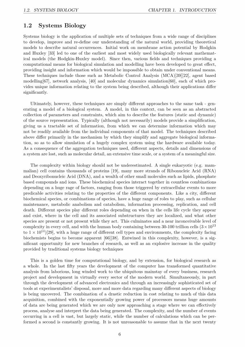
Systems biology is the application of multiple sets of techniques from a wide range of disciplinesto develop, improve and re-define our understanding of the natural world, providing theoreticalmodels to describe natural occurrences. Initial work on membrane action potential by Hodgkinand Huxley [33] led to one of the earliest and most widely used biologically relevant mathemat-ical models (the Hodgkin-Huxley model). Since then, various fields and techniques providing acomputational means for biological simulation and modelling have been developed to great effect,providing insight and information which would be impossible to obtain under conventional means.These techniques include those such as Metabolic Control Analysis (MCA)[39][22], agent basedmodelling[67], network analysis, [40] and molecular dynamics simulation[60], each of which pro-vides unique information relating to the system being described, although their applications differsignificantly.

Ultimately, however, these techniques are simply different approaches to the same task - gen-erating a model of a biological system. A model, in this context, can be seen as an abstractedcollection of parameters and constraints, which aim to describe the features (static and dynamic)of the source representation. Typically (although not necessarily) models provide a simplification,giving us a tractable set of information, from which we can determine information which maynot be readily available from the individual components of that model. The techniques describedabove differ primarily in the mechanism by which they simplify and aggregate biological informa-tion, so as to allow simulation of a hugely complex system using the hardware available today.As a consequence of the aggregation techniques used, different aspects, details and dimensions ofa system are lost, such as molecular detail, an extensive time scale, or a system of a meaningful size.

The complexity within biology should not be underestimated. A single eukaryotic (e.g. mam-malian) cell contains thousands of proteins [19], many more strands of Ribonucleic Acid (RNA)and Deoxyribonucleic Acid (DNA), and a wealth of other small molecules such as lipids, phosphatebased compounds and ions. These biochemical species interact together in countless combinationsdepending on a huge rage of factors, ranging from those triggered by extracellular events to morepredicable activities relating to the properties of the different components. Like a city, differentbiochemical species, or combinations of species, have a huge range of roles to play, such as cellularmaintenance, metabolic anabolism and catabolism, information processing, replication, and celldeath. Different species play different roles depending on when in the cells life cycle they appearand exist, where in the cell and its associated substructures they are localized, and what otherspecies are present or not present while they act. This culminates and a near inconceivable level ofcomplexity in every cell, and with the human body containing between 30-100 trillion cells (3×1013

to 1× 1014)[29], with a huge range of different cell types and environments, the complexity facingbiochemists begins to become apparent [66][38]. Entwined in this complexity, however, is a sig-nificant opportunity for new branches of research, as well as an explosive increase in the qualityprovided by traditional systems biology techniques

This is a golden time for computational biology, and by extension, for biological research asa whole. In the last fifty years the development of the computer has transformed quantitativeanalysis from laborious, long winded work to the ubiquitous mainstay of every business, researchproject and development in virtually every sector of the modern world. Simultaneously, in partthrough the development of advanced electronics and through an increasingly sophisticated set oftools at experimentalists’ disposal, more and more data regarding many different aspects of biologyis being uncovered. The combination of a drastic reduction in cost relating to much of this dataacquisition, combined with the exponentially growing power of processors means huge amountsof data are being generated which we are only now approaching a stage where we can effectivelyprocess, analyse and interpret the data being generated. The complexity, and the number of eventsoccurring in a cell is vast, but largely static, while the number of calculations which can be per-formed a second is constantly growing. It is not unreasonable to assume that in the next twenty

6

CHAPTER 1. INTRODUCTION 1.2. SYSTEMS BIOLOGY

to fifty years, unanticipated advances in science and technology will yield increasingly powerfulelectronics and software. With advanced methods and hardware, there is no reason why in the fu-ture, systems approaching in size to a cell could not be simulated in increasingly fine detail. Whilesystems biology has previously been seen as the blunt end of research, where guestimation meetsill-fitting parameters and too many assumptions are made to create a biologically relevant models,as both the computational power available and our understanding of the systems increase, more andmore of these subtitles can be described. No one is suggesting that systems biology (or indeed thebroader scope of computational biology) should replace wet-lab based research. Instead, however,it can provide an additional angle and guidance tool, suggesting possible avenues for researchers toexplore, avoiding expensive and time consuming research which may never work.

Figure 1.2: Graph describing number of computations per kWh over time ( c©Jonathan Koomey 2011[43])

7

1.3. BIOCHEMISTRY OVERVIEW CHAPTER 1. INTRODUCTION

1.3 Biochemistry Overview

To effectively describe a biological system, there is a need to carefully define the constraints andparameters involved in that system. To understand the context of these factors, it is advisable tohave at least a general understanding of the key components of biological systems. The infinite andrepetitive nature of life is primarily driven by the replicative nature of cells. These act as homoeo-static micro environments to facilitate ideal conditions for a wide array of biological functions. Cellscome together to form multicellular organisms, where different cells have different roles. Additionalcomponents made of protein and/or inorganic material can be exported by the cells to constructhuge, complex structures to provide a framework for more complex life. This is how the humanbody is built - a mass of cells draped around a bone scaffolding, held together by proteinaceousconnective tissue.

Information flow and cellular replication are intertwined by the central dogma of molecularbiology. DNA provides a long-term storage molecule for information, which can be transcribedinto Messenger Ribonucleic Acid (mRNA). mRNA acts as a malleable and short term informationtransfer molecule, and is used as a blueprint by the cells molecular machinery to assemble proteins.A macromolecular polymer of amino acids, proteins come in a huge range of sizes and roles, fromthe relative simple structural protein collagen, a primary component of connective tissue [63] tothe vastly complicated and multifaceted apoptosome complex, responsible for the coordination andcontrol and apoptosis - programmed cell death[1]. Through the manufacturing of different proteins,cells can construct machinery to carry out all the activities they need to perform. Evolutionarypressures have driven the survival of cells whose DNA produces the proteins best suited to carryout the tasks which lead to their survival in the local environment.

1.3.1 Protein Expression

Protein expression is the process of taking a segment of DNA, transcribing the information encodedin that DNA and translating it into a protein. This is a very complicated process, especially ineukaryotes, but for the purposes of this dissertation a short overview of the critical steps is rele-vant. Ligand1 (transcription factor) triggered DNA expression typically occurs through a numberof steps. Initially, the transcription factor binds to a DNA promoter region in a reversible fashion.Once this initial binding has occurred, other transcription factors associated with the DNA-ligandcomplex interact to form the transcription apparatus. With the transcription apparatus in place,it proceeds linearly along the DNA, using individual RNA nucleotides as reactants and convertingthese isolated, individual RNA monomers into a single RNA polymer which is complementary2 tothe DNA section being read. While the RNA polymer is being generated the original promoter-bound ligands may remain bound, or they may dissociate. If they remain bound, the RNA synthesisprocess may repeat, either before the first has finished, meaning two RNA molecules are being builtconcurrently, or some time after. The rate at which this re-starting occurs depends on a numberof factors including nucleotide availability, the ligand species, cell state etc. This is the processof transcription - transcribing the information, previously stored as a DNA sequence, into therelated medium of RNA. Once this has finished, we are left with a newly formed RNA molecule,the mRNA, and this mRNA molecule can then associate with a ribosome.

Ribosomes are massive, complex molecular superstructures which act as protein factories, takingin an mRNA molecule and amino acid monomers and producing an amino acid polymer (protein3. As in an assembly line factory, they have a conveyor belt like organisation, where the mRNA

1A ligand in this context is a small biological species (protein) which binds to a macromolecule (DNA)2The concept of complementarity is non-relevant to this discussion, although is absolutely crucial to the process.

For additional details see [66]3The distinction between peptide, amino acid polymer and protein is subjective. A protein is an amino acid poly-

mer, although in addition to the order of the amino acids (the primary structure) it includes additional information

8

CHAPTER 1. INTRODUCTION 1.4. KINETIC MODELLING

molecule enters into the ribosome through a single entry point and is pulled in a stepwise motionthrough the ribosome. The ribosome scans the RNA as it passes through, and for every three RNAnucleotides translates this information into one of twenty amino acid monomers. That amino acidis obtained from the ribosome’s local environment and is bound to an ever growing chain of aminoacids. This is the process of translation - translating the information from the nucleotide mediuminto the protein medium. Once the full mRNA molecule has passed through, the ribosome releasesthis newly formed polymer, which goes on to form a protein through a number of post-translationsteps, including folding and potentially chemical modification.

1.3.2 Description of Biochemical Systems

As a result of its central role in biology, traditional biochemistry has developed increasingly sophis-ticated techniques for analysing protein-protein interactions. As this research has progressed, moreand more data regarding the network of proteins involved in various processes in the body can besummarized, and using graph theory based semantics and syntax these networks can be visualizedand analysed [11].

Protein Protein Interaction (PPI) networks can be defined as undirected graphs, where nodesrepresent proteins and edges an interaction between those proteins[11]. Such graphs provide a vi-sual, if highly simplistic way to represent the possible interactions in a cell, and databases such asKEGG are beginning to amass relevant information describing these interactions[57]. One of theprimary drawbacks of PPI networks is the lack of directionality associated with the interaction,often because this metric is non-relevant. Biochemical cell signalling pathways can additionally besimplistically described as specialist directed PPI networks, specifying species involved in commu-nication as nodes, and with the direction of communication as directed edges. With both of thesedescriptions we lack any kind of dynamism in our model. While adding weights to directed edgesindicating relative speed of a pathway or strength of an interaction, the values associated with theseinteractions or reactions vary significantly with a wide range of factors. How rates of reactions varyhas been the subject of extensive research over the last fifty years, and today reaction kinetics isat the heart of almost all biochemical processes. By understanding how fast a process is occurring,and what factors determine that speed, new insight into the mechanism behind the process can beexplored. It is this kinetic modelling and analysis our work focusses on.

1.4 Kinetic Modelling

Much of the early organic chemistry relating to reaction kinetics originated in Germany in thelate nineteenth and early twentieth century. There are a number of different ways reaction ki-netics can be modelled, such as Michaelis Menten kinetics[29] or Hill kinetics[31]. This projectfocusses on using mass action ratio based kinetics, initially described by Guldberg and Waage inthe late nineteenth century[28]. This is the simplest kinetic scheme (outlined below) and providesa straightforward starting point for simulations. Additionally, mass action kinetics have been usedin previous studies on model systems similar to the ones developed, and it seemed prudent tomaintain some kind of continuity, allowing the comparison between the results of our simulationswith previously done ones. Although a critical underpinning, we do not focus on thermodynamicshere, as it is considered beyond the necessary scope for this introduction.

The mass action ratio is the simplest measure for rates, and ties thermodynamic and kineticanalysis together. It provides a formal and mathematics description of the basic intuitive idea thatthe more of a reactant you have, the more products you generate, and that this can only happenat a maximum rate. Consider the equation below. Here A and B are reactants and C and D are

in terms of how it is folded (the secondary, tertiary and quaternary structural information). A peptide is a shorter,typically unfolded amino acid polymer, between two and around forty amino acids, although there is no definite cutoff point)

9

1.4. KINETIC MODELLING CHAPTER 1. INTRODUCTION

products, which is to say we combine A and B and they form C and D. a,b,c,d are the stoicheometriccoefficients of the species, and relay information regarding the ratio of molecular species betweenone another. Note these coefficients are specific to this equation, though not unique.

10

CHAPTER 1. INTRODUCTION 1.4. KINETIC MODELLING

aA+ bB ↔ cC + dD (1.1)

With this setup in mind, the mass action ratio defines an equilibrium constant Keq as shownbelow;

Keq = [C]c[D]d

[A]a[B]b (1.2)

Note that here, as in standard biochemical and chemical notation, [A] denotes the concentrationof species A. TheKeq parameter, described here in terms of species concentration and stoichiometriccoefficients can also be described in terms of the forward and backwards reaction kinetics. Thereaction shown in equation 1.1 in fact describes two reactions

aA+ bB → cC + dD (1.3)

cC + dD → aA+ bB (1.4)

For each of these, the rate constant for the forwards reaction (as there is no backwards reactionin these irriversible reactions) is traditionally denoted k1 or kf (for equation 1.3) and k−1 or kr (forequation 1.4). These two constants related to Keq as follows;

Keq = k1k−1

(1.5)

Through subsitution, we can then derive the following equation;

k1[A]aeq[B]beq = k−1[C]ceq[D]deq (1.6)

Which says that at equilibrium, the product of the concentration of reactants multiplied by theforward reaction constant is equal to the the product of the concentration of products multipliedby the backwards reaction constant.

We can further, then, expand these equations to the following equation

reaction_rate = k1[A]aeq[B]beq − k−1[C]ceq[D]deq (1.7)

At equilibrium reaction_rate is 0. However, at non-equilibrium this equation gives a simplereaction_rate equation which follows the mass action laws of chemical kinetics. It is upon thislaw we base our reaction laws in the models. The units of the k1 and k−1 depend entirly on theeuqation at hand, as we must ensure both k1[A]aeq[B]beq and k−1[C]ceq[D]deq are of the same units. Adetailed dicussion is not required here, but to subtract one value from the other they must be thesame type of information. As a result, kinetic constants are tailored to give us the correct values.

1.4.1 Time-course Modelling

With a basic description of mass action kinetics, the equations behind some commonly used kineticmodels, various method for describing a system’s progression through time exist. We can definea model scheme and a simulation scheme. The model scheme defines how the system is describedat the starting point, and the mathematics behind how new values are calculated. The simulationscheme provides an algorithmic solution to solving variables defined by the model scheme, wheresuch a scheme can be deterministic or non-deterministic.

The simplest model scheme is simply one based on mass action kinetics, where each reaction inthe system is described as above, with the reaction rate based purely on the reactants and products.Such schemes fail to model certain systems correctly, but do provide a fast and effective startingpoint for building models.

11

1.4. KINETIC MODELLING CHAPTER 1. INTRODUCTION

Beyond a basic mass action kinetic scheme is the classic and simple example from LeonorMichaelis and Maud Menton’s 1913 Michaelis-Menten kinetic model for enzyme kinetics[50]. En-zymes are biological catalysts, and facilitate a chemical conversion of one or more reactants intoone or more products without themselves being destroyed. In the Michaelis-Menten model, whichhas it’s foundations in mass action kinetics, an enzyme’s reaction rate is determined by a numberof factors, including reactant, product and enzyme concentration, the rate of catalysis, and therates of binding and release of both reactant and product. Michaelis-menten modelling gave riseto the steady-state system description, whereby enzymes reach an equilibrium which responds toincreasing levels of reactant or enzyme. While initial Michaelis-Menten kinetics focussed on simplesystems, the scheme was subsequently extended to include the effect of reaction modifiers (bothactivators and inhibitors), leading to complex but effective equation sets which provide a goodapproximation for a number of systems. A Michaelis-Menten based steady state system providesa good model for many discrete biochemical pathways, especially those relating to metabolism.However, it is ill-suited to the unidirectional and non-linear flow of information associated withsignalling.

Hill kinetics were developed as a method for describing cooperative binding, originally for a lig-and binding to a macromolecule[31] but can more generally be applied to general reactions wherereactants bind in a cooperative manner[29]. Cooperativity is the affect of multiple identical ligandsbinding to one species, where the binding of each successive ligand affects the affinity of subsequentbinding, both positively (higher affinity) or negatively (lower affinity). In a combination of Hilland Michaelis Menten kinetics, Monod Wyman Changeux (MWC) sigmoid kinetics combine thecooperative of Hill kinetics with a Michaelis-Menten structure to take advantage of multi-subunitenzymes where catalytic rate subunit state affects the enzymes overall activity.

π-calculus (or process calculus) provides an additional tool, where a small number of logicalrules, symbols and parameters define the allowed interconversion between species, the species them-selves, their compartments, and all parameters associated with reactions. Developed for modellingcomplex computational systems, deterministic process calculus has had some biologically relevantsuccess[44], although more research has been done into stochastic process calculus (or StochasticProcess Algebra (SPA)). BIO-PEPA[16] provides the relevant semantics and syntax to describebiological systems system, making up for some of the shortcomings of PEPA. PEPA uses an under-lying Continous Time Markov Chain (CTMC) model to provide a stochastic component based on anegative exponential distribution. By using logical descriptors as opposed to hard (real) numbers,a system can be described in qualitative manner more akin to much of the data collected by exper-imental approaches. While BIO-PEPA has been used with some success for simulating biologicalsystems [27], [58] it suffers from a lack of support in terms of user base, software, and models.Despite previous work in our group using BIO-PEPA, after a conclusive review of the state of theart4 the decision was made to move away.

4Included in supporting information

12

CHAPTER 1. INTRODUCTION 1.4. KINETIC MODELLING

Petri-Nets provide another method for discrete and parallel systems description. They arebased on places and transitions, with arcs which connect the two. Places represent objects, andtransitions how objects are inter converted. Each place may hold zero or more tokens, where tokensrepresent the number of objects in existence.

Figure 1.3: Simple diagram of a petri net P1, P2, P3 and P4 are places, with T1 and T2 transitions between them.The solid black circles are tokens [70]

A transition’s activity depends on the arcs connecting places to that transition, and the num-ber of objects at a connected place. Upon a transition, tokens are removed from the source objectand added to the destination object, where the number of tokens added or subtracted dependson the weight of the arc. It requires integral values for tokens, and a number of both metabolicand signal-transduction based systems have been based on Petri nets [26]. However, despite somesuccess they have had limited results with larger systems, providing an over simplification whichinhibits the description of some biological events.

The aforementioned model schemes set out frameworks to describe the components of a system.We touch on a number of the most commonly used approaches, although there are many more notconsidered here. A system described by one of these setups can then be dynamically simulatedusing a number of different approaches.

1.4.2 Deterministic Modelling

Deterministic modelling is the original form of biochemical simulation, and provides a mathemat-ical description which yields the same result each time the model’s values are calculated over atime course. The most commonly used mechanism for such simulations are Ordinary DifferentialEquations (ODEs), where an ODE is solved to describe a species’ concentration through time.

Petri nets can be solved by ODEs[23], although more typically are evaluated simply based onintegral values and progressive basic calculations along a continuous time course for firing. Thisprovides a deterministic implementation of Petri nets, although a stochastic implementation is alsopossible[9].

1.4.3 Non-deterministic (stochastic) Modelling

Following from the previous section, non-deterministic modelling provides some random elementto a simulation, where the same result is not generated if the system is simulated multiple times.The underlying algorithm for many simulation techniques in chemical and biochemical stochasticmodels is frequently based on Gillespie’s algorithm [24] [25].

When Gillespie’s algorithm is not possible then some interface to a Markovian system is typi-cally used. A Markov chain is a system with states which transition between one-another in such away that the following transition depends solely on the current state - i.e. the transition pathwayis memoryless. While a Markov chain has discrete time steps which trigger a (potential) change instate, a CTMC has this memoryless property, but additionally the trigger for state change is nota discrete value, but instead a negative exponentially distributed delay on the action [32]. Thisnegative exponentially distributed delay means implicit probabilities of transition can be derivedfrom the the distribution. CTMC are difficult to work with directly so a number of systems have

13

1.4. KINETIC MODELLING CHAPTER 1. INTRODUCTION

developed, essentially as high level wrappers to underlying CTMC model.

1.4.4 Project Approach

For this project, we have opted to begin with a simple approach and use matlab based ODEsimulations. This decision was motivated by a number of factors. matlab provides a widely usedand well defined interface for running biological simulations. The matlab SimBiology package[49]is well defined, and includes a number of relevant tools, such as automatic model checking, graphgeneration and an easy to use GUI. However, in addition these tools, it provides a powerful script-ing language, allowing the running of complex simulations and analysis in an automated manner.In a previous dissertation, BIO-PEPA was used to carry out simulations, and while the simulationsthemselves generated interesting data, the lack of a scripting back-end made this project pro-hibitively difficult to develop into a high-throughput system[8]. By using matlab we avoid theseissues, getting the best of both worlds, a convenient user interface, a powerful numerical engine,Linux/Mac/Windows portability, and a well developed scripting and programming language.

14

CHAPTER 1. INTRODUCTION 1.5. MONTE CARLO PARAMETER ESTIMATION

1.5 Monte Carlo Parameter EstimationParameter estimation is the process associated with taking a biological model and through somemeans generating system defining parameters, which when applied to that model allow it to behaveas expected. This “expectation” is based on a comparison of the simulated data with experimentaldata, for example comparing the protein concentration time course in a simulation with experi-mentally collected results. The data generation can be done in a number of ways. Parameterscan be initially estimated based on comparable systems, and then fine tuned to generate resultsin line with experimentally derived data. This typically yields one a single parameter set. Analternative method is to use Monte Carlo simulations to generate a random set of parameters,import these parameters into the model, run a simulation with that parameter set and then com-pare the results with experimental data. Where a parameter set has generated results which arefavourably comparable with empirical data, that parameter set is saved, and the process is repeated.

Figure 1.4: Schematic diagram describing the Monte Carlo parameter estimation algorithm

One factor which is often glossed over with regards to parameter estimation is the concept ofparameter set scope. More specifically, (working under the assumption that the model is perfect)even if a parameter set is generated which produces results in line with empirical data, this doesnot mean that the values generate are the real rate constants. They simply represent a set whichwhen used in a simulation generate the expected results, but there may well be many more sets.The number of possible sets which can generate identical results depends somewhat on the system.For example, in a pathway with one hundred species where empirical data exists for just three,there will be more parameter sets which can generate the same results for those three species thanthere would be if there were empirical data for all one hundred. However, in both cases it is likely(although admittedly not a certainty) that there will be many parameter sets which yield identicalresults. While this is true for Monte-Carlo simulations, it also holds up where parameters from anapparently similar model are introduced and fine tuned. Just because two systems appear similar(assume similarity is in terms of pathway topology and/or constituents) there is no guarantee theunderlying mechanics bare any resemblance to one another. While superimposing parameters maybe tempting (and often correct) this new parameter set is not necessarily “the” correct set of values- rather, it represents a member of a larger set of possible parameters.

15

1.5. MONTE CARLO PARAMETER ESTIMATION CHAPTER 1. INTRODUCTION

Figure 1.5: Graphical overview of the concept of multiple sets of functionally equivalent but numerically disparateparameter sets. Note, black concentric circles represent any of the possible parameter sets in the set of workingparameter sets

In assessing parameters generated through Monte-Carlo simulation, therefore, there is a needto compare the working5 parameter sets with one another. If, for example we are able to generateone hundred working parameter sets, and in all of these sets one of the values remains the samethroughout, it is likely this specific variable is crucial, and that this consistent value representspotentially a real number. By analysing statistical indicators between equivalent parameters fromworking sets, a better picture of a model can be obtained. Indeed, if there appears to be nocorrelation, there may be a fundamental problem with the model. However, an in depth analysisof parameters sets generated through Monte-Carlo simulations goes beyond the scope of this paper.

In addition to the concept of sets of parameter sets, we must also accept that our model is asimplification of an incredibly complicated process. Ideally, such a model is biologically relevantif it captures the key determinants in a system. For example, if a signalling pathway is largelycontrolled by ten proteins, all of which are in our model, then the fact that another five hundredproteins have a minor role in regulating that pathway may not have a major impact of the finaloutcome. Bearing this in mind, however, it is important to remember that any numbers generatedby the simulation are simply rough estimates, and not hard numbers.

5Working here is used to describe a parameter set which when applied to a model and that model simulated, theresults generate data which is comparable with experimental results

16

CHAPTER 1. INTRODUCTION 1.6. SYSTEMS BIOLOGY MARKUP LANGUAGE

1.6 Systems Biology Markup Language

SBML[34] has (arguably) become the standard format for describing biological systems. It com-bines a well defined specification with a complete syntax for describing models, as well as a numberof highly developed APIs in a range of languages (C++, Java, C#, Python and matlab), each ofwhich has extensive documentation. Although defined in a language agnostic manner, it’s typicalimplementation is in an Extensible Markup Language (XML) based format. XML is a standardizedmark up language for encoding information into a consistent and machine readable format[13] and isan ideal format for storing structured, periodic data such as that defined by the SBML specification.

Major editions of SBML are called levels, with minor updates termed versions. For this projectwe focus on level 2 version 1 (L2V1), however, higher levels and versions can be mapped down,although lower levels/versions cannot be mapped up. We have chosen to focus on L2V1 as it repre-sents the majority of publicly available of SBML models. Many models are available in higher, moreadvanced versions, but in a number of repositories later formats can be automatically convertedto earlier ones for downloading [56], meaning L2V1 acts as the lowest common denominator forvirtually all models.

Through ever increasing use in systems biology projects combined with it’s open source nature,SBML has developed a large user base as well as a a number of online model repositories, and asignificant number of different software vendors have integrated SBML import and export into theirproducts. By taking advantage of the backwards compatible nature of the format developments,SBML provides a broad, flexible language for defining the features relevant to a specific model orsystem in a consistent manner, without a forced need for overspecification.

1.6.1 Specification Summary

A complete overview of the specification can be found here[34]. An SBML model is structured aslists of one or more of the ten key components outlined below. We included a brief description ofeach of these components and their role. It’s important to note this is a highly superficial overview -the specification document is succinct, clear, and well written and manages to encompass 167 pages.Each component is a list of elements - these lists simply act as containers for the elements storedin them and provide a logical interface for iterators. For each element, assume a non unique name(for easy reference) and a unique ID (for internal model referencing) unless otherwise suggested.

• List of function definitions (optional) - To add clarity to the specification, users can definecommonly used functions here and then refer to them throughout the model

• List of unit definitions (optional) - Where units are not basic unary descriptors (moles,litres, seconds etc.) the user can define multiple-component units (mole/sec, litre3) here andthen refer to them throughout the model

• List of compartments (optional) - Individual compartments can be defined here. Typicallythis may only include the cytoplasm, but may also include the nucleus, vesicles, or any othercompartments. Compartments include a size, the compartment’s units, and a boolean valueto show if their size is held constant through a simulation

• List of species (optional) - Each species, such as proteins, ions, enzymes, small moleculesor conceptual items (such as “protein synthesis”) is represented as a species. Species havea starting amount or concentration, units, associated compartment, and a number of otherattributes

• List of parameters (optional) - Parameters provide a simple element which stores somevalue. This value can change, or can remain constant, and can have units associated with it

17

1.6. SYSTEMS BIOLOGY MARKUP LANGUAGE CHAPTER 1. INTRODUCTION

• List of initial assignments (optional) - Initial assignments are a little different from theelements already encountered - they lack a name or an ID, instead providing a mechanism toset the initial value of a species where that value depends on other factors which cannot bepredetermined. They can be seen as;

species_ID = initial_assignment(p1, p2, ...pn) (1.8)

Where px can be constants or variables determined by an initial assignment, a parameterfrom the model, other species’ initial concentration, or a function with input values

• List of rules (optional) - Rules provide a way to dynamically calculate a parameter ratherthan have it pre-determined. There are three kinds of rules;

– Assignment rule - Used to express an equation which sets a variables value (such as aparameter, species concentration, or compartment size)

– Rate rule - Used to express the rate of change of a variable (such as a parameter, speciesconcentration or compartment size)

– Algebraic rule - Used to calculate a numerical intermediate or temporary value

Like initial assignments, rules do not have a name or ID, but instead simply act on an element,essentially providing an optional extension for that element

• List of constraints (optional) - Constraints are a mathematical description of model as-sumptions which the model must remain under. If during a simulation the constraint is nolonger satisfied, then that simulation is deemed invalid. A constraint might be that no speciesconcentration can become negative (for example)

• List of reaction (optional) - Reactions are by far the most complex element in the SBMLspecification. They consist of a number of sub-elements defined below. Overall they providean element which describes a reaction between one or more species (“reactants”), and theirconversion to one or more species (“products”). The basic reaction object, as well as a nameand an ID, has a boolean value to determine if it is reversible or not, and the compartmentit occurs in

– List of reactants - A list of species which are the reaction’s reactants– List of products - A list of species which are the reaction’s products– List of modifiers - A list of species which are the reaction’s modifiers (both activators

and inhibitors)– Kinetic law - The kinetic law includes an equation to determine the rate of the reac-

tion. This equation can include predefined functions, parameters and species. However,any species used to define the rate must be included in one the aforementioned lists(reactants, products or modifiers).

In addition to global parameters (defined in the list of parameters) reactions can have theirown local parameters, in a list of parameters object associated with the kinetic law. Theseparameters take precedence over global parameters.

• List of events (optional) - Events describe discontinuous, discrete changes made in responseto a certain state in the model. They include a trigger element, which defines what causes theevent to be fired, a list of event assignments, which define what assignments occur in responseto the trigger, as well as a number of other elements such as priority and delay objects whichallow fine tuning.

18

CHAPTER 1. INTRODUCTION 1.6. SYSTEMS BIOLOGY MARKUP LANGUAGE

Figure 1.6: Example of an XML SBML file structure, with the elements described above labelled for clarity. Thecontent here is irrelevant, although included as a demonstration

19

1.7. ASTHMA CHAPTER 1. INTRODUCTION

This overview describes the ten basic components in an SBML file. It is clear that there is infact significant overlap in terms of what can be done to achieve the same result. For example, anevent can be used to set the initial concentrations (by defining a trigger at t=0), or alternatively aninitial assignments could be used. This functional redundancy is not accidental. In the context ofthe rapidly evolving understanding of biological systems and the development of different ways torepresent them, it is impossible for one single system modelling language to include all the requireddetail for all systems without introducing a significant amount of redundancy into the majority ofdescribed systems. SBML, therefore, provides a flexible core for describing the fundamental com-ponents of a system, which can then be built on by other software to include necessary detail whereappropriate, or simply use the optional objects and attributes provided by the SBML specification.This framework does not require over determination where inappropriate, nor does it typicallyintroduce significant redundancy into the model. By providing a relatively flexible specification,SBML provides a framework for structured system description without being overly restrictive interms of what can and cannot be done.

1.7 Asthma

In this section we provide an overview of the molecular characteristics or asthma, with a focus onGC resistant asthma. Much of this content is relevant for our generation of the GC signalling path-way, although is not crucial to understand the project’s development. We include it here primarilyas reference material for those more biochemically minded.

1.7.1 Overview

Asthma is characterized as a chronic disease which affects the respiratory system, inflaming andnarrowing the airways to induce breathing difficulties [54]. Typically, a trigger causes a sponta-neous attack, which may dissipate rapidly (within hours or even minutes), or may last significantlylonger (a period of weeks or even months). Currently affecting 300 million people, that number ispredicted to rise by an additional 100 million by 2025[3]. While the vast majority of suffers keep thedisease in check using inhalable corticosteroids, occasionally in combination with Long Acting βAgonists (LABAs), around 5% of those affected are resistant to this treatment. This small fractiongenerates a disproportionate amount of the costs associated with sever asthma[36]. By better un-derstanding the molecular mechanism associated with this resistance, improved treatment regimesand more effective drugs could be designed to reduce its impact of the quality of life of individuals,as well as the cost burden burden associated with the resistant asthma.

1.7.2 Molecular Mechanism

The asthmatic triggers depends on the individual and the environment, but are typically associatedwith an allergic response, which may be caused or exacerbated by infection (bacterial or viral), orpollution. The systemic inflammatory response has been the subject of extensive research, and isnot considered in detail here. In summary, upon detection of an allergen, mast cells in the tis-sue around the airways release granules packed with inflammatory mediators, including histamine,which interact with the cells in airway tissue (especially those of smooth muscle) to trigger con-striction and an immediate reduction in airflow to the lungs. These mast cells also produce awhole host of other inflammatory signalling molecules (such as prostaglandins, leukotriens, kinins,Interleukin (IL)-4, IL-13 and chemokines) which promote muscular constriction and attract otherimmune cells such as neutrophils, lymphocytes and eosinophils. Additionally, lymphocytes releaseIL-5, macrophages produces Tumour Necrosis Factor (TNF)-α, and a variety of other moleculessuch as neutrophil chemokines, cytokines and growth factors such as IL-6, IL-11 are produced.These inflammatory signalling molecules all cause the surrounding cells to shift into an inflamma-

20

CHAPTER 1. INTRODUCTION 1.7. ASTHMA

tory state, which is primarily regulated by the antagonistic actions of corticosteroids.

Inside the airway tissue cells, this recruitment and activation of immune cells and the expressionof inflammatory signalling molecules triggers a number of processes which lead to the intracellularinflammatory cascade, and is not something considered here. Additionally, there is a demonstrableincrease in the transcription and activation of a number of inflammatory transcription factors, suchas the NF-κB and Activator Protein-1 (AP-1) families of proteins[4]. Both of these are activated bya whole range of inflammatory signalling molecules associated with the asthmatic response. NF-κBfamily proteins are responsible for the up-regulation in expression of a wide range of molecules,such as chemokines, cytokines, growth factors and enzymes[5], while the genes up-regulated byAP-1 are more typically associated with proliferation and survival.

This frequently leads to the chain reaction observed in asthma attacks (a sever and prolongedepisode of restricted breathing caused by the inflammation) - the initial trigger leads to the tran-scription of the critical signalling molecules (such as cytokines, chemokines and interleukins), whichin turn leads to the expression of those proteins involved in the intracellular inflammatory cascade.At the same time, the signalling molecules cause an increase in the expression and activation oftranscription factors such as NF-κB and AP-1.

NF-κB is activated by a wide range of different stimulatory elements through a number of welldefined pathway[6]. Active AP-1 is a heterodimer of Jun and Fos proteins, and characteristicallybinds to the TRE (TBA response element). The formation of the active heterodimer is facilitatedby the Mitogen Activated Protein Kinase (MAPK) family kinase c-Jun N-terminal Kinase (JNK)through a number of phosphorylation events. NF-κB and AP-1 go on to up-regulate transcription ofinflammatory proteins as well as those signalling molecules, causing a positive feedback loop whichmaintains a state of inflammation in the tissue. In addition to this transcription/expression cycle,chromatin remodelling, typically consisting of histone acetylation to relax DNA tension and facili-tate transcription, triggered by CBP (CREB (cAMP (cyclic Adenosine Monophosphate) ResponseElement Binding Protein) Binding Protein) also contributes to inflammatory protein expression[64].

Inflammation is mediated and reduced by corticosteroids. These signalling molecules signalbetween cells (in the extracellular environment), and originate from the adrenal cortex. Syntheticversions provide a much higher dosage in a localized manner through an inhaler, rather than relyingon the circulatory system. They bind to Glucocortocoid Receptors (GR), found in almost all cells,which then dissociate from a Heat Shock Protein (hsp)-90 chaperone protein to form homodimers.The homodimeric protein can now diffuse into the nucleus, where it binds to a GlucocortocoidResponse Element (GRE) in the DNA, where the AF-1 and AF-2 (Activation Function) domainsalter DNA transcription. This is where the interplay between the pro and anti inflammatory signalsoccurs - the ligand bound GR dimer binds and represses transcription of inflammatory and immunegenes, effectively counteracting the activities of NF-κB and AP-1.

Corticosteroids bind to NF-κB directly and indirectly, causing a reduction in the transcriptionfactor’s ability to up-regulate transcription of inflammatory proteins. Additionally, corticosteroidsrepress MAPKs such as Extracellular Regulated Kinase (ERK) and JNK. By inhibiting JNK acti-vation, corticosteroids block the formation of the active AP-1 heterodimer, meaning corticosteroidsimplement a rapid response mechanism to alleviate inflammation both by directly reducing theexpression of inflammatory molecules and by reducing the transcription and activation of pro-inflammatory transcription factors. Dexamethasone, a potent synthetic corticosteroid, was alsoshown to induce MAPK phosphatase-1 (MKP-1) (an inhibitor of MAPK) and as a result reducesp38 activity, a MAPK frequently associated with inflammation.

GRs are phosphoproteins, meaning their state is altered by phosphorylation. With five sites forphosphorylation (Ser113, Ser141, Ser203, Ser211 and Ser226) phosphorylation provides an effective

21

1.7. ASTHMA CHAPTER 1. INTRODUCTION

Figure 1.7: 1. Schematic diagram of GR with LBD (Ligand Binding Domain) and DBD (DNA Binding Domain)highlighted. 2. hsp90 binds to the GR and stops it dissociating from the cell membrane 3. Corticosteroid bind asligands and trigger hsp90 dissociation, releasing GR from the membrane 4. Two free GR bind together as a dimer,and can the bind DNA 5. The AF-1 and AF-2 domains in a monomer (single GR) are highlighted here.

mechanism to control GR activity. Agonist or antagonist binding to GR effects how the receptor isphosphorylated [68], and the phosphorylation state has been associated with a range of functions.Phosphorylation has been shown to affect DNA binding in a promoter dependent manner [18][69],and Ser211 phosphorylation affects ligand binding, nuclear localization and and GR activation[18].Conversely, in another study Ser211 phosphorylation seemed to increase GR functionality [41].MAPK, Cylcin Dependent Kinase (CDK), Glycogen Synthase Kinase 3 (GSK-3) and JNK are allimplicated in the phosphorylation of GR, although the the role (if any) of p38 remains unclear. InHeLa cells (a standard immortal human cell-line used in a wide array of scientific experiments),up regulated p38 lead to a reduced GR activity through some effect on the ligand binding domain.However, mutation in the p38 gene had no impact on this functionality, suggesting a possibledownstream activity relating to GR chaperone proteins or co-activators[62]. However, in humanand mouse lymphoid cells p38 has been shown to directly increase phosphorylation of GR[51].Essentially, this appears to be a highly complicated tissue and species specific mechanism, where ageneral consensus on the role of enzymes and phosphorylation on activity is yet to be determined.

1.7.3 Corticosteroid Resistance

Corticosteroids provide a fast and effective treatment for asthma, and represents the foundationsof the standard regime for managing the disease at a severe level. However, in a small numberof patients even a high concentration of oral corticosteroids is ineffective [48]. Alternative thera-pies, such as targeting IL-4, IL-5 and IgE (immunoglobulin E) has been investigated, but clinicaltrial results were not encouraging [12] [42] [55]. Better understanding corticosteroid resistance inasthma is crucial in developing new and effective treatment strategies for those affected. From aclinical perspective, CSR asthma is typically diagnosed when the condition fails to improve despitelong-term (14-days) use of oral corticosteroids. On a molecular level, a reduced suppression ofIL-4 and IL-5 mRNA in bronchoalveolar tissue has been reported, as well as a greater number ofcells expressing IL-2, IL-4 and IL-13, indicating that cytokine expression profiles may contributetowards the resistance [47]. Peripheral Blood Mononuclear Cells (PBMCs) - blood based cells witha round nucleus such lymphocyte, monocyte, macrophage, but not neutrophil or eosinophils asthese contain multilobed nuclei - display reduced sensitivity to corticosteroid suppression, meaningin CSR asthma patients corticosteroids have a reduced impact of PMBC cytokine release.

22

CHAPTER 1. INTRODUCTION 1.7. ASTHMA

Cortecosteroid resistance appears to be mediated in patients by a number of distinct mecha-nisms, reflecting the complexity of this regulation. In acquired CSR patients, mechanisms includereduced GR expression, reduced affinity of corticosteroids for GR or a reduced affinity of GR forDNA. Indirect mechanisms include a decreased expression/activity of co-repressor proteins andan increase in NF-κB or AP-1 expression. Patients are not GC deficient[20], with serum GC ly-ing in normal ranges[45]. Similarly, no reduction in the gastrointestinal absorption of GC[46] isseen. Patients display elevated levels of pro-inflammatory interleukins[47] in the bronchial tissue,suggesting an inability to effectively respond to the actions of GC. These elevated levels may becaused by p38 MAPK phosphorylation of GR[35], activating the inflammatory response pathway.Additionally, a distinct reduction in p38 MAPK phosphatase expression is seen in CSR patientsafter exposure to GC [23], and dysregulation of JNK and AP-1 both appear to have some role inthe desensitization to GC[36]. We end our overview of the biological mechanism of GC resistancehere, although the extensive reference material highlighted in the section provides ample discussionon the topic. It is clear that this is a highly complex issue, which does not have a “black and white”answer. Indeed, it seems likely that a number of discrete molecular conditions would give rise tothe same physiological lack of response to GC, although many of these diverse mechanisms may infact be mediated by a small number of interfaces between crucial pathways.

1.7.4 Pathway Crosstalk

Understanding signalling crosstalk between different pathways in the context of GCs signalling mayprovide crucial information to help understand the molecular mechanism of CSR asthma. There isexperimental evidence to suggest that in some forms of CSR patients, the cause of this resistanceis a genetic defect which causes a disruption in normal crosstalk between pathways[4]. Histori-cally, rare genetic anomalies have often provided insight into complex molecular mechanisms, soit seems plausible that while dysregulated crosstalk can have serious effects, under normal condi-tions crosstalk provides an underlying homeostatic mechanism which normally maintains a carefulbalance between pro and anti-inflammatory signals. If this is the case, then treating CSR patientswith GC will have no impact on their well being. However, combining GC with components tooffset or correct cross-talk associated problems may allow these traditional regimes to be effective.In the preceding section, we mentioned the possible impact of JNK, AP-1 and p38 MAPK on GCsignalling, and it is this set of key mediators we focus on here.

Crosstalk appears to occur both at the signalling level and at the gene regulation level, meaningboth aspects should be considered[53]. However, the intricacies associated with the crosstalk ispoorly understood. There is a tendency to study pathways as linear routes from trigger to effector,despite this being a poor representation of signalling systems. As a result, the nuances relevant topathway crosstalk offered by many proteins is lost.

23

1.8. PRECEDING WORK CHAPTER 1. INTRODUCTION

1.8 Preceding WorkThis project is the evolution of two sets of work: a previous MSc project carried out by C. Baroukh[8]and a paper published by B. Hendriks, F. Hua and J. Chabot entitled “Analysis of MechanisticPathway Models in Drug Discovery: p38 Pathway”[30].

Hendriks et al. developed a model of the p38 MAPK signalling pathway shown below, andadditional determined a range between which the parameters in the model would lie based ongeneral values for biological reaction kinetics.

Figure 1.8: p38 MAPK model[30] (includes a minor updated - see section 3.2 for further details.

The Hendriks model was developed in the Teranode Design Suite (Teranode Corporation),exported to SBML and translated into JACOBIAN (Numerica Technology). Simulations for pa-rameter estimation were then performed in JACOBIAN, and a number of possible parameter setswere generated. Our starting point for this project, was this p38 MAPK model developed by Hen-driks et al, combined with the parameter ranges they had already determined.

Baroukh’s dissertation was based on using some of the parameter sets defined by Hendriks et alwith the BIO-PEPA language to simulate the p38 MAPK pathway using a BIO-PEPA generatedmodel, running a version of Gillespie’s algorithm. While this was successful, it became obviousthat the overall lack of software support for the BIO-PEPA framework at this time meant thathigh-throughput simulation and analysis with BIO-PEPA was not-practical. Additionally, despite

24

CHAPTER 1. INTRODUCTION 1.8. PRECEDING WORK

having idealized parameters based on the model developed my Hendriks et al. the results of Hsp27Pspecies concentration for a simulation with these idealized parameters using Gillespie’s algorithmbased on the BIO-PEPA model does not match the experimental data provided. In contrast, theJACOBIAN based ODE simulation gives a much closer match, indicating potentially a problemwith the BIO-PEPA simulation framework. However, this has not been explored further, and myin fact reflect a flaw in the JACOBIAN model.

25

Chapter 2

SBMLIntegrator

OverviewIn this chapter we overview one of the key problems encountered early on, and describe the approachand implementation of a software solution. The specifications regarding this problem are considered,general design concepts shown and the software engineering methodologies used are named andjustified. We finish by describing the finished project, evaluating it in the context of our originalgoals, and discussing the future work associated with it.

2.1 Introduction

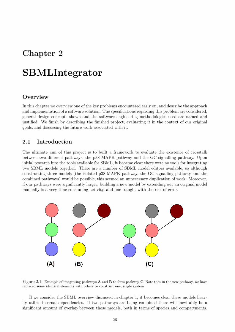
The ultimate aim of this project is to built a framework to evaluate the existence of crosstalkbetween two different pathways, the p38 MAPK pathway and the GC signalling pathway. Uponinitial research into the tools available for SBML, it became clear there were no tools for integratingtwo SBML models together. There are a number of SBML model editors available, so althoughconstructing three models (the isolated p38-MAPK pathway, the GC-signalling pathway and thecombined pathways) would be possible, this seemed an unnecessary duplication of work. Moreover,if our pathways were significantly larger, building a new model by extending out an original modelmanually is a very time consuming activity, and one fraught with the risk of error.

Figure 2.1: Example of integrating pathways A and B to form pathway C. Note that in the new pathway, we havereplaced some identical elements with others to construct one, single system.

If we consider the SBML overview discussed in chapter 1, it becomes clear these models heav-ily utilize internal dependencies. If two pathways are being combined there will inevitably be asignificant amount of overlap between those models, both in terms of species and compartments,

26

CHAPTER 2. SBMLINTEGRATOR 2.2. SPECIFICATION

but also units. Additionally, there is a need to ensure element IDs are unique across both models.Some software check this, but many do not, leading to scoping conflicts. The ID variable is notenforced as unique in the SBML specification to allow for deliberate namespace ambiguity (e.g. forlocal parameters), however, in situations where two models are being combined it can lead to silenterrors which disrupt a model while failing to generate any obvious symptoms. A tool to automatethe integration of two models in a semantically and syntactically accurate manner would speedthis process up immensely, and significantly reduce the risk of human error in what would be anincredibly long winded and tedious process.

A second motivation for developing an automatic integration tool is that biological understand-ing of systems often changes, leading to a need to update models or parameters. Such updates to apoorly constructed integrated system risk breaking the model - small changes can have significantimpact across a model in a cascading effect. Typically the reason for integrating two models willbe to investigate how they interact, which suggests a lack of detailed understanding of this newlyformed integrated model, but a better overview of the two individual models. By ensuring inte-gration is quick and easy, researchers can make changes to individual models and then re-integratethem, rather than navigating through the complex and convoluted task of editing an already inte-grated model in the context of one of its two submodels.

Ultimately, this relates to the concept of least resistance - if a tool is available to make integratingtwo models together easy, then this becomes an appealing research topic. Hundreds of modelsalready exist in the BioModels Database[56], many of which could be integrated and investigated forcrosstalk. The description of biochemical pathways as semi-linear isolated communication networksis largely an inaccurate representation, brought about because it provides an ideal way to teachand understand these pathways. Instead, pathways should be looked at as a smaller subcomponentor a larger multi directional and multidimensional network, and integrating two pathways togetheris a means of enlarging two single fragments of an overall signalling network into one, larger sectionof that same network. This is the role of SBMLIntegrator.

2.2 Specification

Considering the challenges discussed, there were a number of initial high level goals for this software;

FunctionalityThe tool should allow the integration of two models basic1 in a flexible manner, where elementsfrom one model can be added to, replace or be integrated with elements in a second model.

Ease of useA tool should remove all possible semantic difficulties, and where it cannot do so should offer usersthe opportunity to make a decision with a number of options presented. The process of integra-tion may not be trivial, however, the overall goal is to ensure any difficulty arises from biologicalquestions, rather than those relating to SBML semantic or syntax.

Ease of installationOne thing which became clear during the initial overview of the various SBML software availablewas that in almost all cases installation was time consuming and complicated. Frequently, extra(often deprecated) libraries were required, which had to be manually configured, and a range ofother problems. To avoid this our aim is that the user needs to simply run a single “Install” programonce, which will install the libSBML library automatically, and then install the SBMLIntegrator.

1Basic in this sense means a model containing one or more of the following elements: Unit Definitions, Compart-ments, Species, Parameters, Rules and Reactions only.

27

2.2. SPECIFICATION CHAPTER 2. SBMLINTEGRATOR

Use of a configuration fileThe process of determining how to integrate two models is (from a biological standpoint) difficult.By providing a simple configuration file where users can enter the specific parameters regardingtheir model integration, this abstracts much of the decision making away from a live program toone where the user has time to carefully consider their options. Additionally, a separate file avoidstime consuming and repetitive interaction, especially if two models are integrated multiple timeswith small changes to integration settings but not to the species being selected. Ideally, the usershould be able to write a configuration file once, and re-integrate two models instantly thereafter,assuming they do not change the way in which the integration occurs. If they do, however, this issimply a case of updating the configuration file.

Completed in a timely mannerIt is important to bear in mind that this thesis is not primarily a software engineering project. Con-sidering this, despite taking a thorough approach to the development of SBMLIntegrator, there isalso a need to objectively prioritise the features required for this specific project. While generatinga software which can integrate any generic models is key for the long-term success of SBMLInte-grator as an independent software tool, in the short term we have focussed here on basic SBMLmodels, which exclude those which contain constraints, function definitions, initial assignments orevents. However, the overall software structure will be developed so as to ultimately facilitate theintroduction of this functionality. With necessity as the mother of invention, this software was bornof a need to integrate two SBML models together, and the realisation that this may be a moregeneral problem. However, developing a fully fledged software tool to deal with all eventualitieswas not a project objective as such, so while this tool does work for a number of generic cases, itis not all encompassing, although these limitations should be viewed in the context of this project,rather than in the context of the SBML specification as a whole.

28

CHAPTER 2. SBMLINTEGRATOR 2.3. DESIGN

2.3 DesignBased on the high level goals outlined above, we developed an overall initial software structure forthe project. A schematic of this structure is outlined below.

Figure 2.2: Simplified schematic of the software’s architecture, with reference to how it interacts with external files.(1) The integration configuration file (discussed below) defines the integration behaviour, and this information isparsed by the configuration file API. (2) Models are read (and in fact written) by functions provided by the LibSBMLAPI. This API is provided for us, and includes a range of functionality, as well as a complete set of containers withgetter and setter functions for all SBML elements.(3) The configuration file API provides a transparent set of functionsto the rest of the software for getting relevant data from the configuration file. (4) The main software then uses theparameters defined by the configuration file and the data imported from the two models to integrate them togetherand construct a new, integrated model

Figure 2.2 describes how SBMLIntegrator interacts with the three input files it requires. Thetwo models are imported into the software, however, they remain in the containers implemented bythe LibSBML API. Similarly, the configuration file is parsed by the configuration file API, whichstores all the information from that file. The main software acts as a co-ordinator of the data in acontrolled manner, but avoids the issues associated with data ownership, duplication and integrity.The LibSBML API containers are well implemented and provide perfect data structures. Similarly,we use a combination of LibSBML data structures and our own template structures to store theconfiguration file information. By abstracting the stored information into specific modules we helpto clarify the flow of information. The process of integration is by it’s nature complicated, withserious issues surrounding data duplication, data validity and data corruption. By ensuring wemaintain a copy of all original data in a state where it cannot be changed while developing a newmodel in a stepwise, dynamic and deterministic manner, we provide fixed reference points for theintegration process while implementing that integration in a logical and efficient way.

29

2.3. DESIGN CHAPTER 2. SBMLINTEGRATOR

One of our earliest design decisions was to allow integration to proceed through the use of threemodels. These are best described by an example where we are integrating model A and model Btogether. In this example, model A is three times the size of model B. Therefore, we designatedmodel A the base model. The base model is used as a template for the new model being createdthrough the act of integration. The base model is copied, and this copy forms the integrationmodel. Initially the integration model and the base model are identical. However, as we proceedthrough the various integration operations, we change the integration model by bringing in com-ponents from the import model (in this example model B). The import model is typically thesmaller of the two, and from it we introduce new elements into the integration model. Neither thebase nor import models are changed in any way, but instead act as static reference points for theprocess of integration use. We refer to the various models as base, import or integration modelsthroughout this chapter. The three models are outlined below, where a basic overview of howintegration proceeds.

Figure 2.3: Overview of the progressive nature of integration based on the three models outlined previously. (1)We begin with the base and import models. (2) The base model is copied to form an identical integration model.(3) The integration process begins by taking new and unique information from the import model. (4) Following this,duplication and redundancy introduced by the action of importing new elements from the import model is removed.(5) Finally, an interactive integration of elements which contain overlap in their attributes for the new model iscarried out. This may include elements such as new reactions which combine reactants and products of two differentreactions. (6) The integration model is now finalized.

After identifying a good method for model representation, the next question regarding theSBMLIntegrator software was, “What is the best way to integrate two models together?”. On thesurface, this seems a fairly simple question, but as various approaches were investigated it becameclear this was less straight forward than anticipated. There is a need to balance efficiency withusability and flexibility. By committing the user to a specific mechanism of integration we reducetheir ability to do certain things, but equally, by allowing integration to be open and flexible werisk huge redundancy in the software, or worse, data inconsistency. After a number of theoreticalprototypes built as flow charts and then evaluated with both user interaction and time/space com-plexity in mind, we developed the Import Replace Integrate (IRI) mechanism for integration.

30

CHAPTER 2. SBMLINTEGRATOR 2.3. DESIGN

2.3.1 Model Integration

Early in our research into methods for integration, it became clear there are three distinct operationswhich can be implemented to integrate elements from two separate models;

• Import - We can simply import (copy) an element from model A into model B.

• Replace - We can define an element in model A to replace an element in model B. Thisinvolves not only overwriting the element in model B, but additionally scanning throughmodel B and changing any reference to the overwritten element to the new element frommodel A. For example if one one model contained Alice and the other Bob, and we replaceAlice with Bob, then not only would both models now contain Bob (and neither Alice), butany references to Alice (such as “Alice in wonderland”) would now be replaced by Bob (“Bobin wonderland”)

• Integrate - We can integrate two elements together, combining aspects of the elements fromboth model to create a hybrid element. For example, if Alice wore red shoes and Bob worebrown shoes, we could integrate the two together, meaning Alice may now wear brown shoes(and Bob would still wear brown shoes as the integration only affects on of the party).

With these three operations in mind, we can discuss the semantics associated with IRI.

IRI integration is based on the fact that you can quickly predefine elements you wish to importfrom one model into another. Similarly, you can also quickly define elements from one model whichyou wish to use to replace elements in another. This process is the same for any element type - forexample, conceptually, replacing Alice in model A with Bob from model B is the same operationas replacing MAPK in model A with ERK in model B. The type of component which Alice, Bob,MAPK and ERK represent is irrelevant. Moreover, there is only one possible outcome from thisreplacement operation. The same is true for the import operations - the outcome of importing thefirst three species from model B into model A will always be the same.

However, integrating two elements together is not uniformly comparable over all element types,and does not always yield the same result. Compartments have different attributes compared tospecies, and again compared to units, and so on. Additionally, where elements have a number ofattributes we do not pre-determine how we integrate these individual attributes. For example withour previous Alice and Bob example, instead of selecting Alice’s name (“Alice”) and Bob’s shoecolour (“Brown”) we could have selected Bob’s name and Alice shoe colour, or chosen to changeeverything or nothing. As shown below this gives four equally possible an correct outcomes of thesame integration, where Alice and Bob are unique IDs, and each individual has two attributes, aname and a shoe colour;

Figure 2.4: The four possible outcomes if we integrate Bob into Alice (note the directionality here)

Beyond this, it should be clear that the order we carry out our replacement, import and integra-tion operations has profound semantic consequences. If we had previously replace all the referencesto “Red shoes” with “Brown shoes” in Alice’s model our option for integration would be reduced;

31

2.3. DESIGN CHAPTER 2. SBMLINTEGRATOR

Figure 2.5: The two possible outcomes if we integrate Bob into Alice after the “Red shoes” → “Brown shoes”replacement operation

We consider below a more relevant example, where we integrate two models together, each ofwhich has a reaction. This shows how the order of operations impacts the final model in a biologicalcontext.

Figure 2.6: We have two models we wish to integrate, model A and model B, where we designate A the basemodel and B the import model. We wish to integrate these two models together in the following way (A) Importspecies S2B into model A, (B) Integrate RxnA and RxnB, such that the hybrid reaction is [S1A + S2A → S2B +S3A] and (C) Replace cytosol_B in model A with cytosol_A.. Figures 1 and 2 show the initial models. Figure 3shows the integration model after the import of species B. Species B is still in cytosol_B, although in the integrationmodel cytosol_B does not exist, so we represent it’s compartment as a grey environment. In figure 4 we integratethe reactions together, which involves introducing S2B as a product. However, it remains in cytosol_B. Figure 5shows the model after the process of replacing references to cytosol_B with cytosol_A. Nowe S2B is in the correctcompartment, and the models have been integrated successfully

32

CHAPTER 2. SBMLINTEGRATOR 2.3. DESIGN

As shown, to achieve successful integration the order of operations is critical. If we attemptto integrate the reactions prior to importing the species, this is possible, although for a while thereaction will refer to a species which does not exist. This may be risky, as it entirely relies onthe user importing the correct species later. It is this kind of complexity we are attempting toabstract from the user, so this is not ideal. Similarly, if we replace cystosol_B with cytosol_Abefore the import of S2B, then S2B’s “compartment” attribute will still refer to cysto_B. However,cytosol_B does not exist in Model A, and to make the system semantically correct we must re-runthe cytosol_B → cytosol_A replacement operation.

This is a very simple example, and in this case it is obvious how to go about this integrationin a manner that would achieve the correct result. However, when dealing with two large, complexsystems, this process is not trivial. With this in mind, we have defined a specific methodology forthe integration of two models.

2.3.2 Import, Replace, Integrate

Below we describe the defined order of operations in IRI integration;

1. A list of all the elements from the import model are imported into the integration model.This occurs exactly once, and is the first thing to happen.

2. A list of all the replacements from the import model are replaced by elements in the basemodel.

3. Once these two set-up operations have been run, we can begin the interactive integrationprocess. Although not required, the software strongly recommends you proceed the integra-tion in the following order - Unit Definitions, Parameters, Compartments, Species, Reactions,Rules. During the integration process, an element created through an integration operationcan be added to the replacement list with the species from the import model as the targetto be overwritten - i.e. any reference to the import model’s species is corrected to refer tothe newly created integration species. Additionally, this new integration element can eitherreplace the pre-existing element from the base model, or can become a new element in itsown right.

With the model wide import and replacement operations happening once at the start, we beginthe integration operations with the model in as a prepared state as possible. While the importand replacement operations are model wide and automatic, the integration operations are carriedout on each of the ten element types individually. It is possible to integrate all ten element typesback to back. However, it is also possible to re-run the replacement operation between integrationoperations. This is typically not necessary, but may provide a means to recover an error made inthe integration process.

By forcing the initial import and replacement, but allowing for stepwise integration of differ-ent element lists with repeated (but not required) replacement of the up-datable replacement list,there is flexibility in terms of how the integration proceeds, but hopefully not at the expense ofmaintaining data integrity. This IRI integration also has the advantage of facilitating it’s specifi-cation through a configuration file. Using such a file, we can define elements to be imported, pairsto be replaced and pairs to be integrated, pre-defining the actions away from the actual softwareoperations. By providing this separation of definition and action, we create a system which canrepeatedly integrate together similar models very quickly. In an ideal world a configuration filewould not be necessary, and the software would intelligently detect elements which were the same,or seemed relate, to offer replacement or integration options. However, with a total lack of any kindof naming standardisation this is simply not possible2. In addition, the flexible design of SBML

2Biochemical ontological standardisation is a significant research topic, and it is our hope that it will lead tobetter, consistent naming conventions

33

2.3. DESIGN CHAPTER 2. SBMLINTEGRATOR

means two syntactically very different models may in fact describe two similar semantic systems.It us up to the user to identify such a scenario, and act accordingly in the design of a configurationfile.

2.3.3 Development Language

SBMLIntegrator was developed in C++ for a number of reasons. Arguably the most completeand best documents SBML API is for C++. By starting with a well documented and highlyeffective API we avoid many of the low level issues associated with data structures, getters, settersand other functionality provided by the API. C++ is also a language ideal for file stream inputand manipulation at the character level, as required by the configuration file interface, providingenough low level functionality to construct a complete and fault tolerant file interaction system.Finally, many of the existing SBML tools are already written in C++, so should SBMLIntegratorbe absorbed into another, multifaceted tool, this avoids the need for a translation.

2.3.4 Architecture

There are a number of key points relating to the software architecture. The LibSBML API includesan SBML model container class, with container objects for the ten lists described in section 1.4, foreach of the elements stored in those lists, and for any other object appropriate attributes associatedwith those elements. In addition, the API provides getters and setters, as well as functionality toread and write SBML files. Considering this, these predefined container classes were used, withclasses containing pointers to Model objects where appropriate. On the whole, however, we’veattempted to avoid the issue of class ownership. By treating classes primarily as collections ofassociated functionality, with significant parent classes holding model objects, we avoid issues ofdata conflict and duplication.

2.3.5 User Interface

We chose to develop a command line based system, rather than a GUI interface. This was pri-marily motivated by the restrictive time scale of the software development element of this project.However, as this work has unfolded, there is a noticeable absence of a good GUI SBML modeleditor for Linux. Command line editors provide an adequate interface for interacting with highlystructured data formats such as SBML, however, we have designed the software in such a way thatfor a final release a QT GUI can be written as an interface over the underlying systems.

For the interface itself, simplicity is a crucial design factor. Command line based systems havethe potential to be overwhelming and difficult to understand. One of the main aims for this softwarewas to provide a tool which is easy to use - the difficulties associated with model integration shouldbe limited exclusively to questions relating to the biological significance of decisions, not file formatissues, duplication of elements, or clashes between names. Considering this we have adopted anumber of standardized approaches to user interaction. These include having three primary waysof interacting with the software which remain consistent through the software.

34

CHAPTER 2. SBMLINTEGRATOR 2.3. DESIGN

Where multiple options are available, the user can enter a number from a list to select an option.

---------------------------------------Select components to show---------------------------------------[1] ------------ Function Definitions[2] ------------ Unit Definitions[3] ------------ Compartments[4] ------------ Species[5] ------------ Parameters[6] ------------ Rules[7] ------------ Initial Assignments[8] ------------ Constraints[9] ------------ Reactions[10] ----------- Events[11] ----------- ReturnSelect:

Interface 1: User interaction through a list of options

Where one of two options or one of three options are available a selection of A or B (or C)is presented, rather than a number selection. This is a deliberate separation of the user menuinterface, which uses numbers (as shown above in Interface 1) with the interactive integrationoptions (shown in Interface 2, below).

### Please select a name for the compartment ###A ----- MediumB ----- Extracellular_envSelect (A or B):

Interface 2: User interaction where one of two options is available

There are also times where the user must select yes or no to a question. Here, the user is invitedto select “Y” or “N”, although “y” or “n” are also acceptable

Do you wish to do X?

Please select Y/N:

Interface 3: User interaction with a yes or no question

35

2.3. DESIGN CHAPTER 2. SBMLINTEGRATOR

At times the user must enter a number or name - here again we have a similar interface. Whenthe user must (or is advised) to select a element which exists in the model, where appropriate, alist of options is presented.

Please enter the new name for the reaction:Please reselect :

Interface 4: Entry screen for value or string

If the user enters an invalid number, a letter or any other kind of illegal character, a standardizederror message is generated and they can re-try;

**** Invalid selection ****Please reselect :

Interface 5: Typical error message upon invalid input

2.3.6 Configuration File Interface

As mentioned, SBMLIntegrator uses a configuration file to define the elements to import, replaceand integrate. The API for this file was developed to be largely separate from the SBMLIntegrator,providing a common interface for the SBMLIntegrator main classes to interact with data structuresrepresenting the loaded file in a manner that is totally abstracted from the main functionality, andfrom any file I/O manipulation.

The SBMLIntegrate configuration file (referred to as the .conf file in the documentation andfrom here on out) has a regular structure, where for each of the ten element types, we define animport list, a list of paired replacement values and a list of paired integration values. The numbersused in this file refer to the element’s index location in the model. We can determine what thesevalues are using the SBMLIntegrator to explore the model and output the list of elements. Wesuggest configuration file design should be done with the SBMLIntegrator open and being used todetermine the correct index values, although this is not required.

36

CHAPTER 2. SBMLINTEGRATOR 2.3. DESIGN

FunctionDefinitions:Import: [0,1,2,3]Replace: [1,2] [2,3]Integrate: [4,5]

UnitDefinitions:Import: [1,2,3]Replace:Integrate:

Compartments:Import:Replace: [2,3]Integrate:

Species:Import:Replace:Integrate: [4,5]

Parameters:Import:Replace:Integrate:

InitialAssignments:Import: [1,2]Replace: [2,3]Integrate:

Rules:Import: [3,4]Replace:Integrate: [1,5]

Constraints:Import:Replace: [1,1]Integrate: [2,3]

Reactions:Import:Replace:Integrate:

Events:Import:Replace:Integrate:

Configuration file 1: Example configuration file structure

37

2.3. DESIGN CHAPTER 2. SBMLINTEGRATOR

The previous page shows an example of a configuration file, giving a general structure. For thepaired values (replacements and integration) the first value in the pair comes from the base model,with the second from the import model. In the case of the replacement operation, the base modelelement replaces any reference to the import model element in the model. In the case of integrationoperation, the base model element and import model element are combined together.

The .conf file interface uses the keywords Function Definition:, Unit Definition:, Compartment:etc. to act as placeholders for the interface data loader. Once the loader locates these placeholder, ituploads the data following the Import:, Replace: and Integrate: keywords to relevant data structuresin the configuration file API. A more detailed discussion of the approach chosen here is providedin the implementation.

A key feature of the configuration file interface is to ensure the state of the data loaded from thefile is functional. That is, to provide error and warning messages when a configuration file is badlyformatted, and to provide output relating to the data loaded for debugging purposes. Typically,systems which facilitate interactions through a user generated configuration file are exposed toerror based on user input through that file, so it is important to ensure that this interface is wellguarded against incorrect or pathological input.

2.3.7 Log Files

The integration process is also repeatable, so if the user makes a mistake they can re-do the inte-gration, overwriting previous elements to correct the error. One of the potential drawbacks of acommand line interface is that it does not provide any easy mechanism to keep track of a system’sstate. A GUI interface may provide multiple windows or side boxes, where values exist and areupdated in real time to provide an effective at-a-glance evaluation of a systems state. This is notpossible with a command line system. With the model integration process, users may not want tobe informed of every event going on behind the scenes. Indeed, with complex model integrations,one simple decision such as “Replace compartment X with compartment Y ” can results in literallyhundreds of replacement operations. Consistently outputting all of these to the user would beunhelpful, however, the user may also want some manner to review what operations have takenplace, to evaluate a problem with a newly created model and it’s source.

With this in mind, for each integration operation the software generates a log file detailingall events and any potential errors or problems it has encountered. In addition to recording allreplacement, integration, and import operations, it also details the data loaded of data based onthe .conf file, and any problems or errors which occur. For example, if in the configuration fileyou accidentally defined an import compartment as 20 instead of 2, but there does not exist acompartment 20, then the log file will display the following warning.

WARNING - in loading compartments for import from conf file, non-existantcompartment referenced (20). Ignoring...

Log file 1: Warning message for undefined compartment

Similarly however, if we had meant to define “[2]” in the import list, but instead defined “[ ]”,this causes an error to be written to the log file, and the aborting of the software.

ERROR - in conf_preprocess() line 166, two [] back-to-back - this usuallymeans there is missing data!

Log file 2: Error message during configuration file preprocessing

38

CHAPTER 2. SBMLINTEGRATOR 2.4. METHODOLOGY

2.4 MethodologyConsidering the limited time scale to develop the software, it was essential to determine whichcomponents were not relevant to the project and could be left as incomplete stubs. While there isan absolute need to prioritise functionality relevant to this dissertation, this should not be at theexpense of the software architecture. We therefore designed initial classes in a complete manner,leaving non-critical functionality with stubs inside completely built functions, containers or classes,rather than simply not doing it.

The overall time scale for the majority of the coding was four weeks, excluding documentationand installation scripts. With the time frame defined, the critical design and development objec-tives were determined in the context of the overall project’s goals. Based on this high level planwith a real completion date, a high-speed scrum like development process was used. Through this,a set of goals were designated and over a sprint period of around three to four days these goalswere met. Where there were significant problems, the cause of these problems were evaluated,and the implication considered in the context of the remainder of the project. This is reflectedin the implementation of the software. Early design decisions to separate the search and replace-ment class lead to later decisions to separate the classes which carry out import, replacement andintegration. Similarly, despite providing a significant reduction in lines of code, the initial useof a template design pattern in the the cleanup/search classes perhaps made the software moreconfusing that it needed to be. Subsequently, template classes and functions were increasinglyused, while the template design pattern was used less avoiding premature optimisation. This isespecially critical considering a significant portion of this base code may need to be restructuredfor the re-development of SBMLIntegrator into a GUI based tool (not during this project).

2.4.1 Development Tools

Our primary development tool was Emacs, with version control provided by Git. The GitHubrepository for this project can be found at https://github.com/rednaxela/SBMLIntegrator. Wechose Git and GitHub, as they provide an ideal, decentralized mechanism for version control, whichconsidering a number of different computers were used to carry out development, provided an idealmechanism not just to maintain regression versions, but additionally to synchronize developmentacross a number of different devices. Testing was carried out through text-dumps, some basic unittesting and user testing. A number of different biochemical systems were used to give a spread ofdifferent scenarios for integration, although a more complete testing package would be advisableduring beta development.

2.5 ImplementationOn the following page, we include the summary inheritance diagram for the SBMLIntegrator soft-ware structure. Following this, we will briefly describe each class’ role, consider some of the keyfeatures in the implementation and the technical decisions which motivated them. We then overviewthe series of operations which the software performs to take two, separate SBML models and com-bine them into one single model.

39

2.5. IMPLEMENTATION CHAPTER 2. SBMLINTEGRATOR

Figu

re2.7:

Thisinhe

ritan

cediagram

describ

estheba

sicstructureof

ourfin

alim

plem

entatio

nof

theSB

MLIntegrator.

Onthefollo

wingpa

gewebriefly

describ

eeach

classan

dit’s

prim

aryrole

40

CHAPTER 2. SBMLINTEGRATOR 2.5. IMPLEMENTATION

2.5.1 Class Description

The classes are described below in a logical order, although this does not always reflect the orderthey appear in the preceding diagram. As this is not primarily a software engineering project, wewill avoid undue focus on the actual code, although the fully commented source code, complete withseparate class and function documentation courtesy of Doxygen[65] is included in the supportinginformation3.

SBML_formatterThe SBML_formatter class is the root class to all the other classes in the SBMLIntegrator struc-ture. It contains text and data structure formatting tools as well as storing a static output streamcalled the log_stream. This log_stream provides a software wide portal to a single log file, throughwhich any operations, warnings and errors can be reported. A number of system-wide constantsare set here too, as well as simple functions to get data such as time, date, product version etc.This is also where the template function append_to_ID() exists (discussed later).

SBML_UI_generalLike the SBML_formatter class acts as a root class to everything, theSBML_UI_general class acts as a root class to anything which has any possibility of user interac-tion. This encompasses everything except the two container classes SBML_integration_containerand SBML_listpair_container. This class contains generic, user interaction functions which maybe used by any other class, including functionality such as selecting a value, inputting data oroutputting standardized text.

SBML_UI_mainSBML_UI_main provides the core user interface for the main menu, as well as a number of publicuser interface functions (print logo, print version, print usage etc)

SBML_searchThe SBML_search class includes the functionality which allows for the searching through themodel for a specific element. This includes functions to determine if a specific element is present(is_present(...)) or not, as well as a unit definition lookup to give the long form of a unit definition.In addition to simply searching for an element, the search framework uses the template designpattern in conjunction with the cleanup class to provide model-wide replacement of an elementwith an alternative.

SBML_cleanupThe SBML_cleanup class is a child of the SBML_search superclass, and utilizes dynamic bindingof methods in the superclass which bind to virtual functions in either the superclass or subclass,depending on what object type is having the method invoked. The cleanup class has a set ofpublic functions for replacing one element with another (replace(element1, element2)). When thismethod is called it calls the search function locate_and_replace(...). Locate_and_replace is the pri-mary search function in the SBML_search class. However, when called by an SBML_cleanup objectit implements a replacement functionality by calling a virtual function which in the search classsimply returns true (to indicate the target has been found) but in the cleanup class replaces thatelement. Through this we effectively use near identical code to achieve radically different resultswith minimal code duplication.

SBML_augmentSBML_augment is the class responsible for implementing model wide changes. At present, it hasa single role in appending a single string to the end of every ID of every element in the model.This is achieved in part through the template function append_to_ID() found in SBML_formatter.This function takes any element and appends a string onto it’s ID. It is imperative the user does

3Documentation is found the SBMLIntegrator folder under docs. The main page is index.html

41

2.5. IMPLEMENTATION CHAPTER 2. SBMLINTEGRATOR

not pass an element which does not have an ID attribute to this function.

SBML_confInputSBML_confInput is a somewhat different class to the ones encountered so far. It is here we imple-ment the configuration file interface. The file interface works by taking a .conf file and scanningit to ensure it has the ten components expected. Once this has been verified, it re-scans throughthe file, importing the defined values in the import, replace and integrate lists into internal datastructures. With the data from the file parsed, the connection to the configuration file is then closed.

The SBML_confInput object has ten internal container objects (SBML_integration_container). Eachof these containers can store the import list, two replacement lists (where list_A contains the baseelements doing the replacing and list_B the import elements which are to be replaced) and twointegration lists (where list_A contains the elements from the base model, and list_B from theimport model). With the dual lists, the first item in list A and B are a pair, as are the second,and so on. With the data successfully uploaded from the configuration file, the designated ele-ments are loaded into their appropriate lists in each of the SBML_integration_container objects,and then these are stored permanently as internal data objects in the SBML_confInput object.To access the elements of the lists, getter function, providing access to the container through theSBML_confInput object exist, allowing other classes to request the contents of the container objects,with the SBML_confInput acting as a gatekeeper, maintaining the data’s integrity.

SBML_integration_containerAs mentioned, this container acts as a data structure to store five lists of elements. It includesgetters and setters, as well as a function which returns the length of any of the lists. The pairedreplace lists A & B and integrate lists A & B should always be the same length.

SBML_integrateThe SBML_integrate class acts as the controller class for the IRI integration process. It con-tains the user interface menus and houses the interaction which calls upon the classes involvedin import, replacement and integration process. It holds a SBML_confInput object with the .conffile data loaded and provides a means for the SBML_integrate_import, SBML_integrate_replaceand SBML_integrate_integrate classes to access the relevant information. Additionally, it containsten SBML_listpair_container objects, which hold the replacement lists, initially copied from anSBML_confInput object. These provide an efficient manner to pass the replacement list betweenfunctions, and between classes, and provides a dynamic copy which is updated by the integrationprocess as this proceeds.

SBML_listpair_containerThe SBML_listpair_container is a very simple data structure for storing a pair of SBML listOf ob-jects, whatever their element contents may be. It is used to primarily to improve code readabilityand clarity.

SBML_integrate_importSBML_integrate_import takes configuration file Import: lists from SBML_integrate and implementsthe import of the relevant elements from the import model into the integrate model

SBML_integrate_replaceSBML_integrate_replace takes configuration file Replace: lists from SBML_integrate and imple-ments the model-wide replacement of the relevant elements as defined by the two lists.

SBML_integrate_integrateSBML_integrate_integrate takes the configuration file Integrate: lists from SBML_integrate and im-plements the model-wide integration of the relevant elements as defined by the two lists. For all

42

CHAPTER 2. SBMLINTEGRATOR 2.5. IMPLEMENTATION

the integrate_*(...) functions, we step through the various attributes of that element type. If twoattributes are identical (or not present in both) we skip over them. However, if they differ, we canchose one of the two for our new “integration” element. This is true for all currently implementedintegration functions except for reactions. When integrating reactions it is quite probable that nei-ther of the two reactions will obtain the attribute values needed to describe the integrated element.Therefore, where appropriate, the user can define their own value, including kinetic laws, names orreaction constants.

After the integration of an element is complete, the user can select for it to represent eithera brand new element, or an update to the existing element in the integration model. Where theintegration element can be referenced (i.e. it has an ID variable, such as a species or a parameter,but not a rule) then the user can select to add the newly defined integration element and the importelement to as a replacement pair to the replacement list. For example, if they defined a new type ofprotein based on data from two different species, all future references to the import species wouldnow refer to the newly created species.

We include a very basic UML diagram to describe visually how the preceding classes in-teract. Note the classes who’s role is primarily to provide parent functionality (SBML_search,SBML_formatter, SBML_UI_general SBML_integrate_helper) are not included here for clarity

43

2.5. IMPLEMENTATION CHAPTER 2. SBMLINTEGRATOR

Figu

re2.8:

Very

simpleUMLshow

ingthesoftw

arearchite

cture

44

CHAPTER 2. SBMLINTEGRATOR 2.5. IMPLEMENTATION

2.5.2 Functionality Concepts and Implementation

A common theme throughout this development process was the concept of similarity. Frequently,different SBML elements were scanned for a particular string in one or more attributes. Wherepossible, we tried to implement template functions to take a generic SBML elements as arguments,then use a polymorphic LibSBML function to obtain a value, compare that value to the searchtarget, and act accordingly. However, on occasion specific elements were simply too different fromone another to make this approach worthwhile. While our final implementation may not representthe most absolute, code-sparing approach, we have attempted to balance both code clarity andreduction in the form of template functions, with functionality. In some instances, it proved easierto write element-specific functions rather than tailor template functions with specializations.

The use of a template class to store the data from the configuration file enables us to produce asoftware specific dynamic structure on top of the lower level SBML specific containers implementedby the LibSBML API. Through the template functions we define a standard interface for the mainsoftware to interact with the data we import from the two models based on the integration file.The integration file is parsed once, the data used to import all the relative SBML elements fromthe two models, and then those elementes are stored in a dynamic data structure which can growand shrink using the underlying SBML ListOf objects. This provides a quick and efficient way toget the relevant data into a stable state. All the disk I/O occurs at the start in a single block,although we chose to carry out multiple reads of the file in favour of a single sequential read, whichwould require all the data to be in a rigid structure. This represents a significant reduction in disklatency compared to an earlier prototype, where in lieu of storing all the information in memorywe carried out individual reads to the file on request. By avoiding the I/O bottleneck we ensurearchitecturally that the software is optimised, especially for older hardware.

On a earlier prototypes, the ability to select the import and base models on the initial setupwas not included. Instead, the software evaluated which model was the bigger and the more com-plicated, and assigned the larger model as the base model and the smaller as the import model.However, in practice not having control over which is which is not an ideal design feature. It maybe the case that the user simply wishes to import a small number of components from a large modelinto a smaller one. An important design choice is that SBMLIntegrator does not force the userto fully integrate two models. In keeping with SBML’s philosophy of not enforcing specific designdecisions on model builders, it was decided the forcing the complete integration of two models couldreduce usability. Instead, by specifying components the user has the choice of integrating parts ofa model. Of course, it is the user’s responsibility to ensure they components they import ensurethe final model works. However, using the configuration file it is very simple to update the definedmodel integration parameters should they make a mistake on the first integration.

The use of a detailed logfile began as a debugging tool during development. However, it veryquickly became obvious that having an optional detailed output describing the operations thesoftware is carrying out is a valuable tool for model integrators. By being able to see what ishappening behind the scenes, much more effective diagnostics, as well as identifying the need to re-run the replacement operations. This information is not critical to the software’s functionality, andforcing it upon the user would be unhelpful and overwhelming. However, in equal measure - hidingthe complexity to the extent it is not possible to effectively troubleshoot is counter productive. Wehave therefore opted for a "See as much as you want" approach - the user can easily access thedetailed information if they need it, but is not presented with it unless they have a specific need.

2.5.3 Program Operation

We include here a very brief user guide to the software, describing the installation and integra-tion of two models. This is a very brief walk-through, with a more detailed description in theREADME.txt file included with the source code. As one of the software’s objectives, we hope that

45

2.5. IMPLEMENTATION CHAPTER 2. SBMLINTEGRATOR

the process is

InstallationOn this distribution we include the LibSBML API library (used for installation) with the sourcecode, configured to install locally with SBMLIntegrator. In future releases we will offer the optionto configure with a pre-existing LibSBML installation, however, for the dissertation hand in it isparamount to ensure we provide a fully, standalone working software. Installation is simply a caseof running the installation script as follows

COPYING.txt dxygn_config INSTALL.sh README.txt srcdocs example libsbml-5.0.0 scripts

$ sh INSTALL.sh

Interface 6: SBMLIntegrator installation process

Upon running INSTALL.sh the installation package begins by running the predefined configureprocess for LibSBML. SBMLIntegrator piggybacks on LibSBML’s dependencies, meaning we needonly a single configure process for both packages. Should the installation fail during this configureprocess the user will be greeted with an error message and the library missing. Typically we havetested the installation on a number of systems, and found that the only package missing may bethe xml2-config library, an XML parsing library used in favour of the more commonly used Xercesdue to an error in Xerces which could not be worked around by LibSBML. This can be obtainedby installing the libxml2-dev package.

After the successful configuration process LibSBML is compiled and installed, followed by SBM-LIntegator. The installation automatically runs ldconfig, which requires ROOT access. However, ifyou are unable to enter the root password this is not a major problem, and can be skipped. AfterSBMLIntegrator has installed you may receive the following error upon attempting to run run thesoftware;

$ ./SBMLIntegrator: error while loading shared libraries: libsbml.so.5:cannot open shared object file: No such file or directory

Interface 7: Shared object error

46

CHAPTER 2. SBMLINTEGRATOR 2.5. IMPLEMENTATION

Such an error suggest you need to configure the LD path. In a BASH shell this involves adding

export LD_LIBRARY_PATH=<full directory where libsbml/lib is located>:$LD_LIBRARY_PATH

to your .bashrc. Similarly, with csh add the following to your .cshrc file

setenv LD_LIBRARY_PATH <full directory where libsbml/lib is located>

In both these cases the libsbml directory is in the folder you ran INSTALL.sh from after installation.No other potential problems have been encountered, and this extra configuration of theLD_LIBRARAY_PATH variable pertain to the LibSBML installation and configuration, not SBM-LIntegrator 4.

Usage

With the software installed, it is run using the command;

./SBMLIntegrator file [file2]

Interface 8: Running SBMLIntegrator, where file and file2 are .xml SBML files

The software takes one or two files. Typical *nix system flags –help and –version appropriatelydisplay basic help and the software version. If the program is passed a single file it initiates thesoftware into explore-only mode, meaning it acts as a very simple text-based model viewer.

################################################################################## WELCOME TO SBML INTEGRATOR (version 0.1 (alpha)) ##################################################################################

----- SBMLIntegrator - Main Menu -----Select an option from below:

[1] ------------ Explore Models[2] ------------ Display Model Summary[3] ------------ Quit

Select:

Interface 9: Single file input welcome screen

From here the user can explore a model or display a summary of the models parameters. Figuresof these outputs are available in the appendix. To exit the software, the user selects quit. Thisgoes through a process of closing output streams to ensure data integrity of the log file

4For more details on these issues see http://sbml.org/Software/libSBML/docs/cpp-api/libsbml-installation.html

47

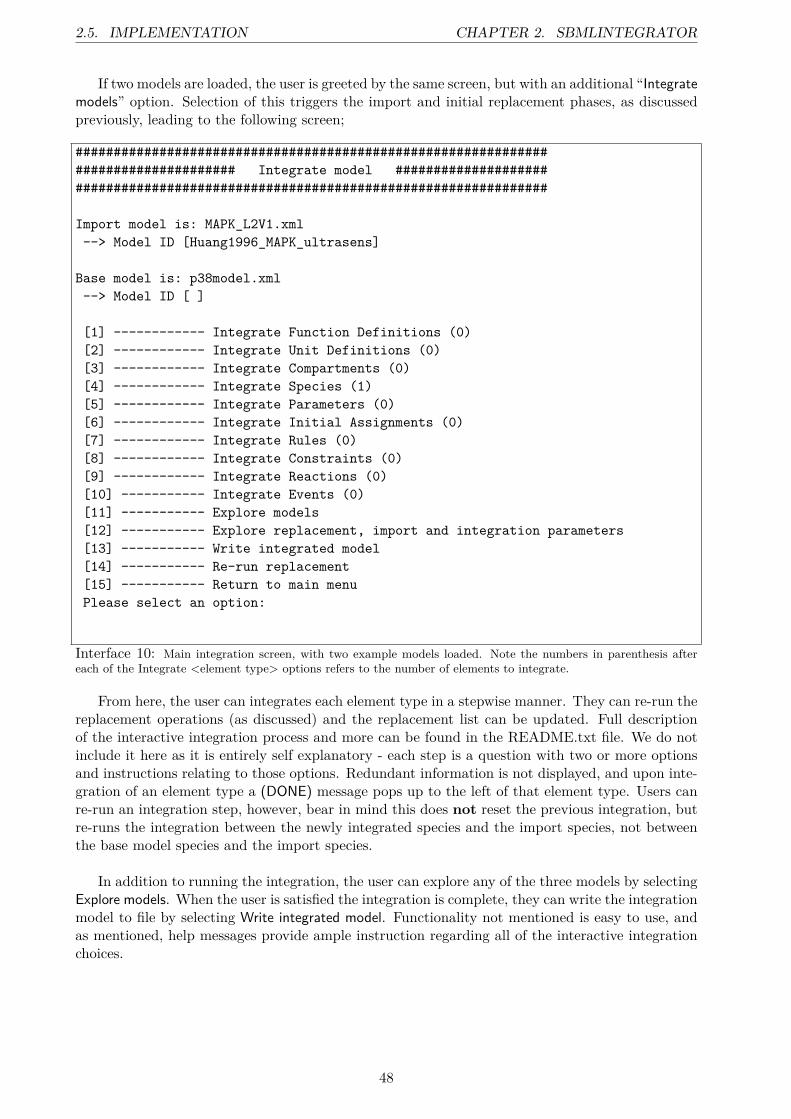
2.5. IMPLEMENTATION CHAPTER 2. SBMLINTEGRATOR

If two models are loaded, the user is greeted by the same screen, but with an additional “Integratemodels” option. Selection of this triggers the import and initial replacement phases, as discussedpreviously, leading to the following screen;

################################################################################### Integrate model ##################################################################################

Import model is: MAPK_L2V1.xml--> Model ID [Huang1996_MAPK_ultrasens]

Base model is: p38model.xml--> Model ID [ ]

[1] ------------ Integrate Function Definitions (0)[2] ------------ Integrate Unit Definitions (0)[3] ------------ Integrate Compartments (0)[4] ------------ Integrate Species (1)[5] ------------ Integrate Parameters (0)[6] ------------ Integrate Initial Assignments (0)[7] ------------ Integrate Rules (0)[8] ------------ Integrate Constraints (0)[9] ------------ Integrate Reactions (0)[10] ----------- Integrate Events (0)[11] ----------- Explore models[12] ----------- Explore replacement, import and integration parameters[13] ----------- Write integrated model[14] ----------- Re-run replacement[15] ----------- Return to main menuPlease select an option:

Interface 10: Main integration screen, with two example models loaded. Note the numbers in parenthesis aftereach of the Integrate <element type> options refers to the number of elements to integrate.

From here, the user can integrates each element type in a stepwise manner. They can re-run thereplacement operations (as discussed) and the replacement list can be updated. Full descriptionof the interactive integration process and more can be found in the README.txt file. We do notinclude it here as it is entirely self explanatory - each step is a question with two or more optionsand instructions relating to those options. Redundant information is not displayed, and upon inte-gration of an element type a (DONE) message pops up to the left of that element type. Users canre-run an integration step, however, bear in mind this does not reset the previous integration, butre-runs the integration between the newly integrated species and the import species, not betweenthe base model species and the import species.

In addition to running the integration, the user can explore any of the three models by selectingExplore models. When the user is satisfied the integration is complete, they can write the integrationmodel to file by selecting Write integrated model. Functionality not mentioned is easy to use, andas mentioned, help messages provide ample instruction regarding all of the interactive integrationchoices.

48

CHAPTER 2. SBMLINTEGRATOR 2.5. IMPLEMENTATION

Code documentation

In addition to the brief discussion on the software code provided here, a far more in depth overviewcan be obtained by viewing the source code documentation. We provide a convenient and easilyaccessible HTML guide created by Doxygen to overview the roles of classes, functions and memberattributes. Above are screenshots of the interface, showing the overall class overview, and thestructure of the class documentation.

Figure 2.9: Main class list page

Figure 2.10: Example documentation, here showing the detailed description of the SBML_confInput function

49

2.6. EVALUATION AND FUTURE DEVELOPMENT CHAPTER 2. SBMLINTEGRATOR

2.6 Evaluation and Future Development

In this section we consider if the SBMLIntegrator in its current form meets our initial objectives.We review the features which were left out in order to accomplish development within the timeframe for our specific purpose, and consider what steps were made to ensure their integration infuture versions. On this topic, we look ahead to the future of SBMLIntegrator, in terms of futurereleases and new features added to the software.

2.6.1 Evaluation of Goals

Below we present an overview of the project’s goals, and the success with which each was met;

Objective Notes EvaluationFunctionality Our software is capable of integrating

two basic SBML models together. Suchmodels do not include initial assign-ments, events, constraints or functiondefinitions. However, these elementsare more advanced features not neces-sary for simple systems biology mod-elling. Integration occurs in a sys-tematic, clear manner, which preservesdata integrity while remaining flexible.

Through extensive user testing ofmodel integrations we believe thesoftware more than adequatelymeets this goals, hugely improv-ing the time it would take to in-tegrate two models by hand.

Ease of use Wherever necessary, help messages andextra information provide supportingguidance through the software. We in-clude the generation of a log file to fa-cilitate easy debugging if necessary, butavoid an overwhelming amount of in-formation where it is not required

We believe the software is intu-itive and easy to use, and thatthe complexity relating to the in-tegration process has been ab-stracted to biologically relevantquestions exclusively

Ease of installa-tion

Installation requires a single command,with potentially the addition of a file tothe LD Path.

We believe the software offers avery straight forward and com-pelling installation process

Use of a configu-ration file

A configuration file is used to define theelements to import, replace and inte-grate. A well defined API for readingthe file and accessing the parsed datawas developed, which as well as mak-ing data access straight forward for thesoftware, provides a number of errorchecking and defensive programmingstrategies against mal-formatted files

A configuration file is used

Completed in atimely manner

We deployed a regimented developmentprocess to ensure deadlines were metand a product was produced on time.The development of the installationprocess took considerably longer thanexpected, however, despite this the ver-sion deployed meets our other objec-tive and was completed well before theproject’s September 9th deadline

The project was successfullycompleted without becoming anoverwhelming burden on the dis-sertation

Table 2.1: Evaluation of SBMLIntegrator’s goals

50

CHAPTER 2. SBMLINTEGRATOR 2.6. EVALUATION AND FUTURE DEVELOPMENT

2.6.2 Future Work and Long Term Goals

The current SBMLIntegrator version does not presently permit the integration of complex systems5.These are more advanced modelling features which were not part of our models, and represent func-tionality and semantics ignored matlab. Therefore, had these elements been included in the modelsthere would have been a need to remove them again before they could be simulated. Despite notincluding functionality relating to the integration of these elements, we have structured the softwareas if they exist, with the source code including the completed function calls, devoid of content. Anearly future update to the software will be to include functionality relating to these elements, andallow their integration.

At present, the software can only deal with L2V1 models. While this represents the lowestcommon denominator, it would be preferable to facilitate multiple levels and versions of support.As a result of the backwards compatibility of SBML, this could be easily facilitated through in-heritance, whereby a base class would allow the integration of L2V1, with progressive subclassesallowing for the integration of later SBML versions. Virtual functions and dynamic binding couldspecify version specific behaviour where different approaches are required depending on the version.

A better user interface is a primary objective for the version 1 release. Through discussion withthe SBML community we are identifying desirable features for a simple, fast SBML model viewer,editor and integrator. Adding complete model editing power to SBMLIntegrator is a natural stepforwards, although was not one of our initial goals, and considering the time frame was deliberatenot attempted in this project. In addition, we are looking at taking the underlying functional coredeveloped here, and implementing a QT framework GUI above it to allow fast and effective userinteraction. The command line approach is adequate for this project, and indeed has proven to benecessary to allow us to complete the software in time. However, with more time, a GUI interfacehas a number of significant advantages over a command line one, and we hope in the monthsfollowing this project to complete and push out a fully functional GUI based version to meet theneed identified during the early phases of this project. Additional discussion on the future workrelating to SBMLIntegrator can be found in section 6.2.3.

5Where a complex system contains one or more of the following element types: Function Definitions, InitialAssignments, Constraints or Events

51

Chapter 3

Model Development

In this chapter we describe our development of an integrated p38 MAPK-GC signalling pathway.Although quite a short chapter it was a significant part of the project, as it required a extensiveamount of background research. Ultimately, we present an entirely new SBML model, which wehope will in the future help demonstrate the existence of crosstalk between the p38 MAPK andGC signalling pathways.

Early in the project, we held discussions with Professor Ian Adcock, who planned to carry outwet lab experiments to obtain empirical data relating to the species defined in our model. The hopewas that by comparing the data generated through Monte Carlo parameter estimation simulationswith the real, empirical data, we would be able to identify parameter sets which, upon simulationusing our model, would generate results in line with the available experimental data. By comparinghow those parameter sets change when the two pathways are integrated (specifically in relation tothe p38-MAPK pathway) we hope to identify any impact the GC pathway has on the p38 MAPKpathway and vice-versa, which would be indicative of the crosstalk suggested in the introductorychapter.

3.1 GR Pathway Development

As described in figure 1.8, our starting point was the p38 MAPK model developed by Pfizer.A number of possible related pathways were considered for exploration and development in thecontext of the p38 MAPK pathway. These included the Interleukin-2 (IL-2), Interleukin-4 (IL-4)and Interleukin-13 (IL-13). Research suggested the IL-13 may be one of the crucial mediatorsof asthma[71], however upon research into pathway structure it was determined insufficient dataexists to generate an effective model. Similarly, despite their potential role, both IL-2 and IL-4have extensive roles in a number of other processes[52], suggesting that any simplified pathwaywould have fundamental and potentially overwhelming flaws due to the absence of any interactionwith typical cellular components. GCs, however, have a much more specific role, and are almostexclusively associated with the anti-inflammatory response, and it is with this activity that theyfulfil their role as a treatment for chronic asthma.

With this in mind, the GC pathway seemed an ideal starting point for designing a complemen-tary signalling pathway which could be merged into the previously designed p38 MAPK pathwaymodel. Developing a new model pathway is not an easy task. There are necessary simplificationswhich must be made to make the process tractable, and identifying the core pathway componentswhile avoiding unnecessary periphery can be impossible when data is lacking. For this development,an extensive and broad research phase was carried out, looking at the various possible componentsin the GC pathway. In this development process, there is a need to carefully balance model com-plexity with completeness; if the model is too simplistic we miss out on key nuances which givecharacteristic system behaviour. Inevitably a model will be far more simple than the biological

52

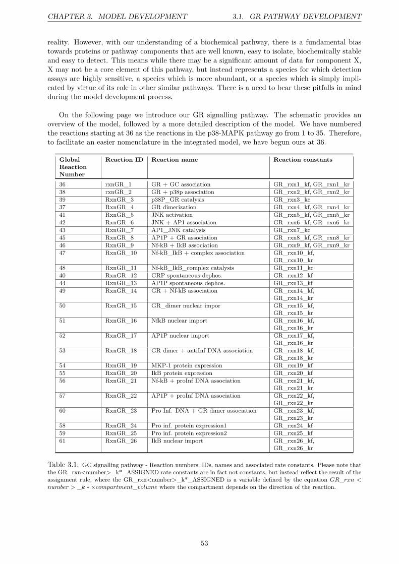
CHAPTER 3. MODEL DEVELOPMENT 3.1. GR PATHWAY DEVELOPMENT

reality. However, with our understanding of a biochemical pathway, there is a fundamental biastowards proteins or pathway components that are well known, easy to isolate, biochemically stableand easy to detect. This means while there may be a significant amount of data for component X,X may not be a core element of this pathway, but instead represents a species for which detectionassays are highly sensitive, a species which is more abundant, or a species which is simply impli-cated by virtue of its role in other similar pathways. There is a need to bear these pitfalls in mindduring the model development process.

On the following page we introduce our GR signalling pathway. The schematic provides anoverview of the model, followed by a more detailed description of the model. We have numberedthe reactions starting at 36 as the reactions in the p38-MAPK pathway go from 1 to 35. Therefore,to facilitate an easier nomenclature in the integrated model, we have begun ours at 36.

GlobalReactionNumber

Reaction ID Reaction name Reaction constants

36 rxnGR_1 GR + GC association GR_rxn1_kf, GR_rxn1_kr38 rxnGR_2 GR + p38p association GR_rxn2_kf, GR_rxn2_kr39 RxnGR_3 p38P_GR catalysis GR_rxn3_kc37 RxnGR_4 GR dimerization GR_rxn4_kf, GR_rxn4_kr41 RxnGR_5 JNK activation GR_rxn5_kf, GR_rxn5_kr42 RxnGR_6 JNK + AP1 association GR_rxn6_kf, GR_rxn6_kr43 RxnGR_7 AP1_JNK catalysis GR_rxn7_kc45 RxnGR_8 AP1P + GR association GR_rxn8_kf, GR_rxn8_kr46 RxnGR_9 Nf-kB + IkB association GR_rxn9_kf, GR_rxn9_kr47 RxnGR_10 Nf-kB_IkB + complex association GR_rxn10_kf,

GR_rxn10_kr48 RxnGR_11 Nf-kB_IkB_complex catalysis GR_rxn11_kc40 RxnGR_12 GRP spontaneous dephos. GR_rxn12_kf44 RxnGR_13 AP1P spontaneous dephos. GR_rxn13_kf49 RxnGR_14 GR + Nf-kB association GR_rxn14_kf,

GR_rxn14_kr50 RxnGR_15 GR_dimer nuclear impor GR_rxn15_kf,

GR_rxn15_kr51 RxnGR_16 NfkB nuclear import GR_rxn16_kf,

GR_rxn16_kr52 RxnGR_17 AP1P nuclear import GR_rxn17_kf,

GR_rxn16_kr53 RxnGR_18 GR dimer + antiInf DNA association GR_rxn18_kf,

GR_rxn18_kr54 RxnGR_19 MKP-1 protein expression GR_rxn19_kf55 RxnGR_20 IkB protein expression GR_rxn20_kf56 RxnGR_21 Nf-kB + proInf DNA association GR_rxn21_kf,

GR_rxn21_kr57 RxnGR_22 AP1P + proInf DNA association GR_rxn22_kf,

GR_rxn22_kr60 RxnGR_23 Pro Inf. DNA + GR dimer association GR_rxn23_kf,

GR_rxn23_kr58 RxnGR_24 Pro inf. protein expression1 GR_rxn24_kf59 RxnGR_25 Pro inf. protein expression2 GR_rxn25_kf61 RxnGR_26 IkB nuclear import GR_rxn26_kf,

GR_rxn26_kr

Table 3.1: GC signalling pathway - Reaction numbers, IDs, names and associated rate constants. Please note thatthe GR_rxn<number>_k*_ASSIGNED rate constants are in fact not constants, but instead reflect the result of theassignment rule, where the GR_rxn<number>_k*_ASSIGNED is a variable defined by the equation GR_rxn <number > _k ∗ ×compartment_volume where the compartment depends on the direction of the reaction.

53

3.1. GR PATHWAY DEVELOPMENT CHAPTER 3. MODEL DEVELOPMENT

Figure 3.1: Glucocorticosteroid signalling pathway. GC binds to the inactive GR-inhibitor complex, causingthe release of the inhibitor and activating the GR. The GR monomer can bind to p38P, where p38P then phospho-rylates and inactivates the GR. It can also bind the active AP-1P transcription factor, sequestering it and downregulating it’s pro-inflammatory impact. Similarly, it also sequesters the NF-κB transcription factor to reduce it’spro-inflammatory effects. Finally, the GR can also dimerize, forming a dimeric transcription factor. This GR dimerundergoes bidirectional transport into the nucleus where it binds to anti inflammatory genes and triggers anti inflam-matory protein expression, including the expression of MKP-1, the p38P dephosphorylase and IκB, the NF-κB specificinhibitor. In addition to this positive transcription regulation, GR can also bind to pro inflammatory genes, inhibitingthe binding of transcription machinery and blocking their expression. AP-1P, mentioned previously is formed throughAP-1 phosphorylation which is catalysed by JNK. AP-1P is dephosphoryalted by a number of proteins, an similarlyJNK is activated and deactivated by a number of different factors, this includes both positive and negatively actingphosphorylation and displays extensive tissue specificity. To simplify this, we describe JNK’s activation/inactivata-tion and AP-1Ps dephosphorylation as a simple first order reversible reaction. If AP-1P remains active and is notsequestered by GR it can undergo nuclear transport and bind to pro-inflammatory genes, triggering the expressionof generic pro-inflammatory proteins. TAK1 complex can phosphorylate the NF-κB-Iκ complex, releasing NFκB-Iκfrom it’s inhibitory subunit and allowing it to move into the nucleus, where, like AP-1P, it triggers the expressionof generic pro-inflammatory proteins after binding to pro-inflammatory genes. For the process of protein expression,we combine transcription and translation into a single process, treat all nucleotides as an unlimited pool at a fixedconcentration, and consider the only factor which impacts gene expression to be the transcription factor in question.This is a gross simplification, but will suffice for an initial model.[6][7][4][5][35][48][53][62][51][41][14][21][10][37][2]

54

CHAPTER 3. MODEL DEVELOPMENT 3.1. GR PATHWAY DEVELOPMENT

The model is similar to the p38 MAPK model in a number of respects. We deliberately choseto model conversion reactions as a reversible forwards association step, and a second, irreversiblecatalytic step. For example p38P and the active GR associate together in reaction 38, and thisGR_p38P complex can either collapse back to it’s constituent reactants, or progress through thecatalytic reaction (39) to form the phosphorylated GR (GRP), while the p38P species remainsunchanged. It is important to not that these reactions fail to account for molecular mechanisms inany way, nor do they include the affect of modifiers on the reactions.

In addition to the proteins, the GR pathway includes DNA expression regulation. To describeprotein expression in such a simplistic system is difficult. The process of DNA expression is highlycomplicated, and the effect of positive and negative regulation very delicate, complex and multi-faceted. We have attempted here to define a simple approximation for DNA expression, using thesame underlying principles used for protein-protein catalysis. For a review of the core componentsof protein expression see section 1.3.1. We represent the binding of transcription factors such asthe GR dimer, NF-κB and AP-1P to DNA as association reactions, similar to the protein-proteinones described previously. However, we can estimate the concentration of anti inflammatory andpro inflammatory DNA to a much more narrow range compared to the ranges of protein species,based on the fact that the number of relevant genes can be far more accurately estimated than theconcentration of a protein. The number of genes remains static, and is consistent for all cells in anorganism, while protein concentration is dynamic, and varies widely in a cell specific manner.

As the foundation for our range, typical multi-target transcription factors my bind around 10different genes with common promoter or enhancer regions. From this we can estimate there arearound 10 proteins which can have their expression directly triggered through (say) GR dimerbinding to DNA (we assume one gene-one protein hypothesis, ignoring RNA processing). We mustestimate the number of nucleotides which GR can use to recognize the promoters of the relevantproteins. This is difficult, as it not only depends on the DNA sequence, but also DNA structure. Asa rough estimate, we suggest 40 nucleotides either side of the promoter region, plus 8 nucleotidesfor the promoter itself. Based on this estimate, each of the 10 DNA sequences where GR dimercould bind includes 88 nucleotides, meaning there are 880 possible nucleotides that GR dimer couldbind to and correctly associate with the promoter. These are rough estimates, largely based ongeneral trends and not pertaining to a specific target. We need to determine a general range oforders of magnitude to begin the parameter estimation process, and depending on the outcome wecan change this range as seems appropriate. Do not consider these numbers hard values.

Using Avogadro’s law we can determine the number of moles;

Na = N

n≡ n = N

Na≡ n = 880

6.023× 1023 = 1.4611× 10−21mol (3.1)

Using the nuclear volume as 1×10−13 we can then calculate the concentration of relevant DNA;

c = n

V≡ c = 1.4611× 10−21

1× 10−13 = 1.4611× 10−8mol/l (3.2)

This gives a concentration of around 0.015µmol, placing it within an equivalent range of ofthe concentration of protein species, although somewhat lower than the majority of species, as wewould expect. To achieve biochemically relevant DNA binding at this concentration, the kon forGR dimer would need to be at the top end of the range of kon, with second order forward rateconstants around 1×106M−1. Indeed, such a kon rate constant would be consistent with a numberof empirical studies evaluating promoter association rates[15][59]. Compared to protein species, theconcentration of relevant DNA is static, and although this concentration estimation is effectivelyno more than an educated guess, it does represent a value which can be quantitatively checkedand updated easily, and is likely to be far more consistent between cells irrespective of tissue. Forsimplicity, we assume a concentration one order of magnitude around 0.01µmol.

55

3.1. GR PATHWAY DEVELOPMENT CHAPTER 3. MODEL DEVELOPMENT

The empirically defined association rates of DNA and transcription factor give an estimatedrange of between 104 and 109. However, the process of transcription uses a number of molecularclamps and other mechanisms to ensure that once transcription begins the process continues untilcompletion. For our model this is not the case - here this association rate determines the concentra-tion of DNA:transcription factor which in a gross simplification is then converted in a single reactionto transcription factor and expressed protein. Considering this, the ranges for DNA-transcriptionfactor association should higher than the empirical values predict, and should correlate with therate of protein expression to ensure it is statistically likely for proteins will ever be expressed.

The rate of protein expression can be less accurately estimated based on empirical data, as wecondense both transcription and translation into a single, mass action based reaction. Initially weattempted to define a range based on available empirical data. However, it very quickly becameclear that a huge number of factors1 make such an estimation for our simplified and condensed“gene expression” reaction impossible. Instead, we consider the reaction in the context of thismodel and simulation, as opposed to the reaction in the context of the empirical data associatedwith the phenomena. Choosing an (empirically) realistic low rate constant would be incorrect, assuch rate constants simply describe the rate at which nucleotides are transcribed, or amino acidspolymerized. However, for this reaction we are simplifying the DNA and the transcription factor totwo, single species, which combine and produce two species. We must therefore give the reaction arate constant appropriate for a simple chemical reaction, not a the empirical data associated withgene transcription and translation.

With this in mind, we define the DNA-transcription factor association rate as between 108 and1011 M−1 min−1, meaning the DNA has a very high affinity for the transcription factors. We definethe reverse reaction as between 10−6 and and 10−1 min−1, reducing the dissociation rate by halfthat of other reaction ranges. We then define the forward protein expression rate as being between10−4 and 100 min−1. This is a lower range than other reactions, meaning that proteins will still begenerated (as the DNA-transcription factor is a super-stable complex) but this generation shouldoccur at a significantly reduced rate compared to other reactions. The nucleotide concentrationis then also defined with the same range as normal species, except they remain constant throughthe reaction by setting their boundary conditions boolean attribute to "TRUE". This reflects that,except under exception circumstances, nucleotides do not represent a limiting factor the proteinexpression, and our model does not include the pathways necessary to generate more nucleotides

A final comment of the values presented here - these simply represent a starting point tonarrow the search space. They are educated, intelligent guesses, based on a significant amount ofbackground work and experience. They are a starting point from which we can build a model,and hopefully using empirical data begin to improve and enhance the range and model description.Other rate constant and initial concentration ranges were based on the values used by Hendriks etal[30] to maintain model parity between the two models.

1Factors include tissue specificity, species specificity, oxidation state, growth conditions, gene, transcription factor,and post translational modification

56

CHAPTER 3. MODEL DEVELOPMENT 3.1. GR PATHWAY DEVELOPMENT

Compartment Name Lower conc Upper concmedium medium_GC 10−3 102

cytosol cytosol_GR_inactive 10−3 102

cytosol cytosol_p38P_GR 0 0cytosol cytosol_GRP 0 0cytosol cytosol_GR 0 0cytosol cytosol_GR_dimer 0 0cytosol cytosol_JNK_inactive 10−3 102

cytosol cytosol_JNK 0 0cytosol cytosol_AP1 10−3 102

cytosol cytosol_JNK_AP1 0 0cytosol cytosol_AP1P 0 0cytosol cytosol_NFkB 0 0cytosol cytosol_IkB 0 0cytosol cytosol_NFkB_IkB 10−3 102

cytosol cytosol_NFkB_IkB_complex 0 0cytosol cytosol_NFkB_GR 0 0cytosol cytosol_p38P 0 0cytosol cytosol_AP1P_GR 0 0cytosol cytosol_complex 0 0nucleus nucleus_MKP1 0 0nucleus nucleus_IkB 10−3 102

nucleus nucleus_NFkB 10−3 102

nucleus nucleus_GR_dimer 0 0nucleus nucleus_nucleotides 10−3 102

nucleus nucleus_antiInfDNA 10−3 10−1

nucleus nucleus_antiInfDNA_GR_dimer 0 0nucleus nucleus_proInfDNA 10−3 10−1

nucleus nucleus_proInfDNA_NFkB 0 0nucleus nucleus_proInfDNA_AP1P 0 0nucleus nucleus_proInfDNA_GR_dimer 0 0nucleus nucleus_proInfProteins 0 0

Table 3.2: Initial concentrations. Non zero values originate either from ranges determined byHendrix et al, or (in the case of DNA) based on our discussion on the previous page.

57

3.1. GR PATHWAY DEVELOPMENT CHAPTER 3. MODEL DEVELOPMENT

Name Description Rxn Lower Upper UnitsGR_rxn1_kf GR_inactive:GC association rate 1 104 107 M−1 min−1

GR_rxn1_kr GR_inactive:GC dissociation rate 1 10−4 101 min−1

GR_rxn2_kf GR:p38P association rate 2 104 107 M−1 min−1

GR_rxn2_kr GR:p38P dissociation rate 2 10−4 101 min−1

GR_rxn3_kc p38P catalytic rate on GR 3 10−2 102 min−1

GR_rxn4_kf GR dimerisation rate 4 104 107 M−1 min−1

GR_rxn4_kr GR un-dimerisation rate 4 10−4 101 min−1

GR_rxn5_kf JNK activation rate 5 10−4 101 min−1

GR_rxn5_kr JNK inactivation rate 5 10−4 101 min−1

GR_rxn6_kf JNK:AP1 association rate 6 104 107 M−1 min−1

GR_rxn6_kr JNK:AP1 dissociation rate 6 10−4 101 min−1

GR_rxn7_kc JNK catalytic rate on AP1 7 10−2 102 min−1

GR_rxn8_kf AP1P:GR association rate 8 104 107 M−1 min−1

GR_rxn8_kr AP1P:GR dissociation rate 8 10−4 101 min−1

GR_rxn9_kf NfkB:IkB association rate 9 104 107 M−1 min−1

GR_rxn9_kr NfkB:IkB dissociation rate 9 10−4 101 min−1

GR_rxn10_kf TAK1:NFkB_IkB association rate 10 104 107 M−1 min−1

GR_rxn10_kr TAK1:NFkB_IkB dissociation rate 10 10−4 101 min−1

GR_rxn11_kc TAK1 catalytic rate on NfkB_IkB 11 10−2 102 min−1

GR_rxn12_kf Spontaneous GRP dephosphorylation 12 10−4 101 min−1

GR_rxn13_kf Spontaneous AP1P dephosphorylation 13 10−4 101 min−1

GR_rxn14_kf NfkB:GR association rate 14 104 107 M−1 min−1

GR_rxn14_kr NfkB:GR dissociation rate 14 10−4 101 min−1

GR_rxn15_kf GR dimer nuclear import rate 15 10−4 101 min−1

GR_rxn15_kr GR dimer nuclear export rate 15 10−4 101 min−1

GR_rxn16_kf NfkB nuclear import rate 16 10−4 101 min−1

GR_rxn16_kr NfkB nuclear export rate 16 10−4 101 min−1

GR_rxn17_kf AP1P nuclear import rate 17 10−4 101 min−1

GR_rxn17_kr AP1P nuclear export rate 17 10−4 101 min−1

GR_rxn18_kf GR dimer:antiInf DNA association rate 18 108 1011 M−1 min−1

GR_rxn18_kr GR dimer:antiInf DNA dissociation rate 18 10−6 10−1 min−1

GR_rxn19_kf MKP-1 protein expression rate 19 10−4 100 min−1

GR_rxn20_kf IkB protein expression rate 20 10−4 100 min−1

GR_rxn21_kf Nf-kB:proInf DNA association rate 21 108 1011 M−1 min−1

GR_rxn21_kr Nf-kB:proInf DNA dissociation rate 21 10−6 10−1 min−1

GR_rxn22_kf AP1P:proInf DNA association rate 22 108 1011 M−1 min−1

GR_rxn22_kr AP1P:proInf DNA dissociation rate 22 10−6 10−1 min−1

GR_rxn23_kf Pro Inf. DNA:GR dimer association 23 108 1011 M−1min−1

GR_rxn23_kr Pro Inf. DNA:GR dimer dissociation 23 10−6 10−1 min−1

GR_rxn24_kf Pro inf. protein expression1 rate 24 10−4 100 min−1

GR_rxn25_kf Pro inf. protein expression2 rate 25 10−4 100 min−1

GR_rxn26_kf IkB nuclear import rate 26 10−4 101 min−1

GR_rxn26_kr IkB nuclear export rate 26 10−4 101 min−1

Table 3.3: Reaction constant ranges and units, ranges based on work by Hendriks et al. and ourestimations

58

CHAPTER 3. MODEL DEVELOPMENT 3.2. P38 UPDATE

3.2 p38 UpdateThe original SBML file provided as supporting information by Hendriks et al. provides an excel-lent starting point for the p38 MAPK model. It does, however, require some changes to make itusable, as in its current state it fails both to conform the SBML L2V1 specification as well as therequirements which allow it to be simulated in matlab. This was a tedious process of removing asignificant amount of redundancy, and restructuring the way reaction rates were calculated. In theoriginal p38 model2, kinetic laws for reactions were defined as a variable, with that variable set byan assignment rule. We reformatted the model so reaction rules were simply the rules themselves,avoiding an unnecessary intermediate assignment.

Reaction constants in the updated p38 model3 have the format main_P_<type>_<species>.These are the true constants for the reactions. However, the “constants” actually used in the rateequations have the format main_<compartment>_<reaction-number>_<type>, and are in factnot constant. For clarity, we refer to them as applied values. These applied values are insteadassigned on each time step through the simulation by an assignment rule, generally of the formula;

[main_ < compartment > _ < reaction− number > _ < type > = main_P_ < type > _ < species >](3.3)

For the majority of the rules, this introduces unnecessary redundancy. However, it allows us tomaintain a single constant, but add additional factors the change the applied value. This is bestdemonstrated by the nuclear import and export reactions, where the rate is crucially dependent onthe nuclear and cytoplasmic volume.

[main_cytosol_Rxn135_Kf = main_P_ki_p38P × comp_cytosol] (3.4)

Additionally, the model provides all units of time as seconds, while their paper uses minutes.To accommodate for this we converted all units which use seconds into minutes by multiplying by0.016. To ensure consistent units throughout, we converted the LPS concentration from ng/ml intoMolar. This is not strictly necessary, however it means the rate constants for the LPS + TLR4reaction are in equivalent and comparable units to the rest of the model. 10 ng/ml evaluates to1×10−11 or 100nM assuming an LPS molecular mass of 100 kDa[8]. This also changed the range ofvalues which the rate constant could be at, although the units stated are describe as ng/ml/Min−1,it is our belief that this should in fact read 1/(ng/ml)/Min to give a unit consistent model. As aresult, the range is transformed from between 1×10−4 and 1×107 to between 1×10−5 and 1×106.Finally, the diagram shown in figure 2.2 is not identical to the one produced by Hendriks et al. Wehave made a small but crucial adaptation to change reaction 4 from

TAK1_complex_inactive→ TLR4 (3.5)

to

TAK1_complex_inactive→ LPS : TLR4 (3.6)

It is the author’s opinion that the original diagram contains an error. If the inactive TAK1Complexcould degrade TLR4 alone, this would represent an irreversible exit point for LPS from the system.In the original SBML model provided by Hendriks, the reaction uses formula 3.6, not 3.5. We havetherefore opted to use this in our model.

2p38model.xml in supporting information3p38_idealized_model.xml in supporting information

59

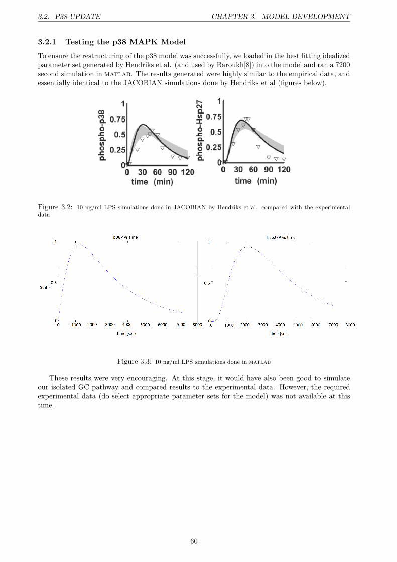
3.2. P38 UPDATE CHAPTER 3. MODEL DEVELOPMENT

3.2.1 Testing the p38 MAPK Model

To ensure the restructuring of the p38 model was successfully, we loaded in the best fitting idealizedparameter set generated by Hendriks et al. (and used by Baroukh[8]) into the model and ran a 7200second simulation in matlab. The results generated were highly similar to the empirical data, andessentially identical to the JACOBIAN simulations done by Hendriks et al (figures below).

Figure 3.2: 10 ng/ml LPS simulations done in JACOBIAN by Hendriks et al. compared with the experimentaldata

Figure 3.3: 10 ng/ml LPS simulations done in matlab

These results were very encouraging. At this stage, it would have also been good to simulateour isolated GC pathway and compared results to the experimental data. However, the requiredexperimental data (do select appropriate parameter sets for the model) was not available at thistime.

60

CHAPTER 3. MODEL DEVELOPMENT 3.3. INTEGRATION PROCESS

3.3 Integration ProcessWith our isolated GR model complete, we used the SBMLIntegrator software described in chapter2 to integrate our GR model with with the p38 MAPK model. After the significant discussionregarding integration theory in chapter 3 we will not go into detail on how this was accomplished.Instead, we include the integrate.conf file in the supporting information, which details the integra-tion parameters used.

As the GC signalling pathway was constructed with the specific purpose of being integratedwith the p38 MAPK pathway, there were no species or reactions to integrate. Designing theconfiguration file4 took five minutes, and running the integration was essentially instant. The easeat which these pathways can be re-integrated through the use of the same configuration file (orhave their integration parameters updated) allows us to easily make changes and updates to themodels individually and then re-run the model integration. This has proven to be invaluable, as wemade a number of minor changes and corrections from the original integrated model. We includea full diagrammatic schematic of the integrated model on the following page.

4Included in supporting information as integration/integrate.conf

61

3.3. INTEGRATION PROCESS CHAPTER 3. MODEL DEVELOPMENT

Figure 3.4: Integrated p38 MAPK - glucocorticosteroid signalling model - For details of the p38 pathwaytopology please see the paper by Hendriks et al. For details on the GC topology see figure 3.1

62

CHAPTER 3. MODEL DEVELOPMENT 3.4. THE INTEGRATED MODEL

3.4 The Integrated ModelThis model is relatively self explanatory, it combines the models defined in figure 1.8 and figure3.1 into a single model. There are a number of positions along the pathway where crosstalk couldoccur. p38P provides a crucial integration point between the pathways, and is formed by theaction of both MKK3 and MKK6 on p38. p38P binds to active, monomeric GR and phosphory-lates it into an inactive form, essentially acting as an off switch for the GC signalling pathway.Similarly p38P binds to and phosphorylates the TAK1 complex into an inactive state, meaningp38P has an antagonistic impact in the two pathways - the TAK1 complex leads to inflammation,while the active GR down regulates it. However, we should consider the species role in the in-dividual pathways to consider the ultimate role of p38P in the integrated pathway. In the p38pathway, p38P acts to trigger inflammation, and it’s role in deactivating TAK1 is one of negativefeedback, a regulation control on the pathway to avoid a run-away inflammatory response. In theGC signalling pathway, however, p38P is a pure antagonist to GC’s activity, and has no further role.

A second, related interaction point between the two models is that of MKP-1 in the nucleus.Active GR forms dimers which move into the nucleus. Here they trigger the expression of antiinflammatory proteins include MKP-1, the p38P phosphorylase. The increased MKP-1 expressioncauses an increase in the rate of p38P dephosphorylation into an inactive state in the nucleus,helping to down-regulate it’s nuclear activities.

Finally, the TAK1 complex interacts with the IκB - NF-κB complex to release NF-κB. IκBsequesters NF-κB, stopping it from causing pro-inflammatory DNA expression. By freeing NF-κB,the TAK1 complex promotes the expression of of pro-inflammatory proteins indirectly. Active GRbinds to and sequesters NF-κB, stopping it from promoting pro inflammatory expression.

Despite having just three points where the pathways interact, they are on three crucial proteins.By comparing the affect of LPS and dexamethasone (a synthetic GC) on the levels of variousproteins, we hope to use this pathway to propel the qualitative and quantitative investigation intoMAPK-GC crosstalk. To use these pathways, we have developed a set of scripts to carry outMonte Carlo parameter generation and evaluation. By comparing the outcome of simulations runwith the data generate by these scripts with real experimental data, we hope to begin to generateputative parameter sets. By evaluating how these sets change in response to different experimentalconditions, we hope to gain insight into the signalling process involved.

63

Chapter 4

Parameter Generation

In this chapter we discuss the final phase of this dissertation, the generation of parameter sets, thesimulation of the models, and their evaluation. We consider our design process for the matlabscripts which implement these tasks and consider any difficulties and how we overcame them. Withthe technical description of these scripts complete, the resulting simulation results are described,and the implications of these results considered. It should be noted the primary purpose of thisproject was not parameter estimation and evaluation. If this were the case, the following chapterwould require a far more rigorous approach in terms of the underlying statistics, the mechanism ofparameter generation, and the evaluation of the generated results. Instead, this phase was originallypart of a means to asses the validity of the integrated model, as well as potentially demonstratethe existence of crosstalk between the two signalling pathways (p38 MAPK and the GC signallingpathway) in the integrated model as described in the preceding chapters. However, the experimen-tal data required to biologically contextualize the integrated model was not obtained, and so as aresult crosstalk evaluation was not possible.Despite this, we include the following discussion, as with the exception of this experimental data,this project is completely prepared to run our Monte Carlo parameter estimation scripts and assessthe generated parameter sets. It is our hope that as soon as this data becomes available, thisassessment can begin.

We do not include a discussion on the concepts behind the Monte Carlo parameter estimationhere, please refer to section 1.5 for further details. Instead, we evaluate our scripts, describing theirdesign and implementation and evaluate their efficiency.

4.1 MATLAB Script OverviewBelow we include a structural overview of the driver script which facilitates the process of parametergeneration1. The script can be seen as two halves, a set up half, were parameters are defined, datais loaded, and the system is prepared for the impending Monte Carlo simulation, and a simulationhalf. In matlab Code 1 we describe, this first part, while the second is described in matlab code2. We use a combination of matlab pseudo code and comments to convey the modularity of theprocedure, while ensuring the process remains clear and conceptually tractable.

1Included in supporting information as /monte_carlo_simulation/additional_information/parameter_estimation_skeleton.m

64

CHAPTER 4. PARAMETER GENERATION 4.1. MATLAB SCRIPT OVERVIEW

% |||||||||||||||||||||||||||||||||||||||||||||||||||||||||||||||||||||||||% SETTINGS

% Model settings

% Model settings are those relating to the overall model. We set the file% name for the model and the replacement number.

% Species Settings

% Settings defining species related parameters. We set some species numbers% and concentrations of our variables such as LPS and Dexamethason

% Simulation Settings

% Things specific to the ODE simulation and parameter generation steps.% We define the number of Monte Carlo loop iterations, the simulation length,% the max timestep and how we generate random numbers

% Ouput Settings

% Output settings are those relating to what data we output, and the system% we’re running on (Windows or Linux)

% |||||||||||||||||||||||||||||||||||||||||||||||||||||||||||||||||||||||||% LOADING DATA

experimental_data = load_experimental_data(...)

normalized_experimental_data = normalize(experimental_data)

model = load_SBML_model(filename)

% |||||||||||||||||||||||||||||||||||||||||||||||||||||||||||||||||||||||||% PRE-SIMULATION SETUP

set_formatting_for_windows_or_unix()

% Determine concentration of any species not in Molar (i.e. LPS is in% ng/ml, so we convert it).

determine_concentrations(...)

% Set simulation settings, including ODE solver to be used (ode23s),% the relative max tolerance (1e-02) and all the settings you defined% in the "settings" bit earlierset_simulation_settings(model)

[missing_initial_concs, missing_params] = identify_missing_parameters(model,replacement_number)

check_file_structure()preconstruct_matrices()

matlab Code 1: Script part 1/2: Setup, loading and initialization

65

4.1. MATLAB SCRIPT OVERVIEW CHAPTER 4. PARAMETER GENERATION

4.1.1 Setup, Loading and Initialization

SettingsThe settings provide the input for users using this script to define variables. It should be notedthese scripts are very much specific to specific models, although there are some parameters the usermay want to alter which are included in the settings section of the script. Below is a summary ofthose settings and a description of each;

Variable Descriptionmodel_name Name of the .xml SBML file to be uploadedreplacement_number Value used by the script to identify parameters which are to be generatedp38P_species_number Model index number for p38PHsp27P_species_number Model index number for Hsp27PLPS_species_number Model index number for LPSLPS_concentration Concentration of LPS in ng/mlLPS_molar_mass Molar mass of LPSN_montecarlo_iterations Number of Monte Carlo loop iterationssimulation_length Number of simulation seconds to runmax_timestep Maximum time step through simulationrandomization_type Type of randomization used (1,2 or 3)plot_graphs_on_success Record .fig of P38p and Hsp27p data for working setsresults_folder Name of folder for outputthreshold_val Sensitivity threshold for good parameters (-1 to 1)windows Working in windows (true/false)unix Working in a *Nix environment (true/false)

Table 4.1: Settings for matlab script

Loading dataHere, three types of data are loaded into the system. The times at which samples were taken asa row vector, one or more sets of experimental results themselves, also as a row vector (wherethe number of elements in the time points vector must equal the number of elements in the re-sults vector), and the SBML model itself, which is loaded based on the file name defined in settings.

Pre-simulation setupIn this section we carry out all the pre-simulation checks, conversions and set ups. This includessetting the ODE configurations, identifying the number of species in the model and carrying out anyunit conversions to ensure parameters are homogeneous in terms of units. We also check to see if afolder exists with the defined folder name - if it does not we create one, so it is imperative the user ofthe scripts has write permission in the defined output folder. We also use the replacement_numberdefined in “Settings ” to create a matrix which contains the index location of the parametersand initial concentrations which require random values to be generated for them. The variablereplacement_number acts as a place-holder to represent, “This value must be generated”, whichby default we set to 99999. When the user is creating a model to simulate in this script theyadd this value into any parameter or initial concentration attribute they wish for a random valueto be generated. Using the identify_missing_parameters(model, replacement_number) function, wescan through the loaded SBML model, and wherever we find an instance of the value, we indexthe location of that initial concentration or parameter in the model. This generates two matrices,one for all the indexed initial concentrations (missing_initial_concs) and one for all the indexedparameters (missing_params). We must use a numerical value as this number because the SBMLspecification ensures that values in parameters or initial concentration must be of type double.However, by hard coding in we run the (somewhat unlikely) risk of replacing a real value which isactually 99999. It is the users responsibility to ensure the replacement_number does not clash withany real values in the model.

66

CHAPTER 4. PARAMETER GENERATION 4.1. MATLAB SCRIPT OVERVIEW

% |||||||||||||||||||||||||||||||||||||||||||||||||||||||||||||||||||||||||% MONTE CARLO SIMULATION

for 1 to number of loop iterations% Generate a random set of parameters for the model based on the missing% initial concentrations and parameters defined in the pre-simulation setup[new_conc, new_param] = generate_parameters(missing_initial_concs,

missing_params,randomization_type)

% Load newly generate initail_concs and parameters into the modelmodel = load_model(new_conc, new_param, model);

% RUN SIMULATION!try

[t,x,names]= sbiosimulate(model);catch error

keyboardcontinue

end

% Normalize all the resultsnormalized_results = normalize(results)

% Compare the results with any experimental data you havegood_value = compare(normalized_experimental_data, normalized_results)

% If a parameter set generates good results, save it and the loaded% model to results/<parameter_set_number>_<date>if (good_value)

save_data()

% If not then discardend of for loop

matlab Code 2: Script part 2/2: Simulation, evaluation and recording or data

4.1.2 Simulation and Evaluation

matlab Code 2 describes the second half of the script, where the parameters are generated, thesimulation run and the results compared with our pre-loaded empirical data. Thegenerate_parameters(...) function takes the missing_initial_concs and missing_params variables, andgenerates random parameters between a predefined range for that specific indexed variable. Thismeans that generate_parameters(...) has the specific ranges and the index location for each pos-sible parameter hard-coded in, and forms the primary basis of why this script is totally modeldependent. By hard-coding these ranges and index locations we avoid a massive amount of pro-cessing to lookup each value, although as a trade-off we do lose portability in terms of other systems.

In addition to passing the missing_initial_concs and missing_params variables, this function alsotakes a randomization_type variable, which should be a value between one and three. This providesthree different ways to generate random numbers.

• Type 3 is a standard random number generator generating a uniformly distributed valuebetween a defined range. For example, a random number between 1 × 101 and 1 × 104 is

67

4.2. PARAMETER GENERATION RANGES CHAPTER 4. PARAMETER GENERATION

almost always on the order of magnitude of 1 × 103. The problem with this is that whenyou have significant ranges of values (such as between 1 × 10−5 and 1 × 106 the probabilityof getting a value less than 1 × 102 is incredibly low. This places an unjustified bias on theupper end of the range of values offered.

• Type 2 is a similar implementation, except it rescales the range to be between 1 and a value,generates a random integer in that range, then rescales that integer back to an appropriatevalue. For example, if you were to generate a random number between 1×107 and 1×108, itrescales this range to be between 1 and 10, generates a random int between 1 and 10 (say 4)and rescales this back to be 4× 107. This does not change the distribution of numbers, butit does limit the number of possible numbers.

• Type 3 is a different implementation which introduces it’s own bias but gives a much broaderrange of values. Here, the range of exponents is determined, and a random integer within thatrange determines the exponent of the returned value. We then generate a random numberbetween 0.1 and 0.999999, which is multiplied by 10 to the power of the new exponent. Fora range between 1 × 10−5 and 1 × 106, this means there is an equal probability of getting avalue on the order of magnitude of 1× 10−5 and 1× 105. The disadvantage here is that thisbiases our average value towards the lower end of the range, as in reality there are “more”numbers between 1000 and 10000 then there are between 1 and 10. However, for the sakeof generating a wide range of values for a simple randomization function in this context itperforms fine, and for that reason the default randomization_type is 3. When types 1 or 2are used the types of results are very similar on every parameter set generation, however, amuch wider range of results (including working sets) are generated by type 3.

Once we have created our matrix of new values the load_model(new_conc, new_param, model)function loads these new values into the model at their correct locations. With this complete weuse the aptly titled simulate(model) function to run the ODE simulation using matlab’s built inODE simulator. The default simulator used is the ODE23s - chemical reactions are notorious forproviding stiff ODEs[61], and our system can afford to use crude error tolerance - there is not aspecific correct value to determine. ODE23s is ideal for such a system, and although other enginescould be used we would highly recommend against it. The simulated(model) function is enclosedin a try/catch block for easy access if a parameter set causes the system to stall. For example, ifthe parameter set triggers matrix convergent errors or the system stiffness prohibits progress, sug-gesting the parameter set is not valid, the user can press [ctrl + c] to abort the simulation. Thistriggers an exception, meaning we jump into the catch block and invoke the keyboard command,transferring control to the user. We could then select enter “resume”, which causes us to jump tothe next loop iteration or “dbquit” which aborts the entire script. Without the keyboard methodcall we would be unable to quit the simulation midway through without forcing matlab to quit.

The normalize_results(results) rescales the results into a normalized form, and thencompare(normalized_experimental_data, normalized_results) uses a simple combination of interpola-tion from the simulation data to the experimental time points followed by a coefficient cost functionto determine how similar the results are. If the results are above a certain threshold then we con-sider this parameter set to be acceptable. The data associated with this run (the parameter set,model, coefficient values for all comparisons, and graphs of those comparisons) are saved, and thenprocess repeats, generating a new random set of values and running the simulation with thosenewly created values loaded into the model.

4.2 Parameter Generation Ranges

The ranges for our parameters originate from both the original p38 MAPK model and from ourown work as discussed in tables 3.2 and 3.3 (GC model) and appendix B1 and B2. These ranges areused as input to the randomizer function in the generate_parameters2.m file. For the rate constant

68

CHAPTER 4. PARAMETER GENERATION 4.3. SIMULATIONS RUN

values, on each loop iteration, a random values is generated which lies within these ranges. Forthe initial concentrations, the same is done, except only for the species which have a non-zeroconcentration to begin with (as described by the aforementioned tables and appendices).

4.3 Simulations RunWe ran simulations of p38 MAPK pathway at 1, 10 and 100 ng/ml LPS. Simulations used athreshold value of 0.88, and ran 50 000 Monte Carlo iterations, with a max time step of 100s,leading approximately 72-100 data points per variable per simulation. We present our results ofthese simulations in the following section. The ability to select parameter sets depends entirelyon the availability of experimental data. We had initially expected to obtain data relating to thepathways under the following experimental conditions;

LPS ng/ml Dexamethasone MAPK inhibitor1 Absent Absent10 Absent Absent0 Present Absent1 Present Absent10 Present Absent1 Absent Present10 Absent Present0 Present Present1 Present Present10 Present Present

Table 4.2: Varying experimental conditions

These experiments were originally to be run and the results collected in good time (July), butunfortunately various problems meant that this data was not able to be obtained. This was unfor-tunate - without this data were were unable to run physiologically contextualized simulations of ourintegrated pathway. However, using the experimental data generated by previously by Hendrikset al. we were able to run the p38-MAPK simulation to ensure our new p38 MAPK model was valid.

In addition, we used our parameter generation algorithm to generate all of the relevant param-eters and concentrations for our integrated system, and using the original p38 data ran a numberof simulations of the integrated system to check it’s biological validity. Such a system is not phys-iologically relevant - the p38 data is for experimental results where no GC were present, while ourintegrated system includes GC . However, despite not being physiologically relevant, running theintegrated system like this has two major advantages. We are able to confirm that our integratedmodel runs, that it has been correctly implemented and does not consistently crash, hugely disruptthe p38 results, or give wildly unexpected results. Secondly, assuming the system works correctly,we can check that it is behaving as expected by examining the concentration of inflammatoryprotein over time. Based on our models, we would expect the level of pro inflammatory proteinsto increase - there is no mechanism for their reduction, although they do not interfere with thereaction in anyway, acting essentially as biomarkers for the model’s progress. It is predicted thatif the integrated pathway is proceeding correctly, the concentration of pro inflammatory proteinswill increase (at different but steady rates) through the course of the simulation.

69

Chapter 5

Results and discussion

We include here some of the data generated by our simulations. All the parameter sets, the completemodels and a range of other data is provided in the supporting information. Because of the lackof experimental data and the overall aims of this project, the discussion of these parameter sets isbrief. The rate constant values are discussed exclusively, as is their impact on the concentrationtrajectory (that is, how a species’ concentration varies across the simulation), while the initialconcentration values do not at this stage add any significant discussion. Some of the implicationsof these results are considered, although any detailed statistical analysis is avoided. The purpose ofthese simulations is not the generate parameter sets for analysis (although another project wouldno doubt find a wealth of information of interest here) but instead as qualitative tools to test thevalidity of both the re-structured p38 model, and our integrated p38-MAPK model. The resultsshould be biochemically relevant, match previous work, and meet our expectation defined in theprevious section.

5.1 p38 MAPK SimulationsThree p38 MAPK simulations were run, with critical simulation parameters defined below;

Simulation [LPS] (ng/ml) # parameter sets # loop iterations Corr. threshold1 1 53 50000 0.882 10 95 50000 0.883 100 240 50000 0.88

Table 5.1: Summary of p38 MAPK simulations

A subsection of the concentration graphs produced by the p38 MAPK simulations are included.These graphs show the concentrations of specific species over time generated by every parametersets which was determined functional based on existing experimental data. These concentrationspectrum graphs provide a qualitative overview of the progression of various species over all theoperational parameter sets. The objective here is not to analyse these data individually, but insteadto use the graphs as qualitative tools from which we can gain insight into the model, the variabilityon each of those species’ and ensure the progressions meet our expectations.

70

CHAPTER 5. RESULTS AND DISCUSSION 5.1. P38 MAPK SIMULATIONS

Figure 5.1: p38P concentration spectrum. Plot (A) describes the concentration at 1 ng/ml LPS, while plot(B) is at 100 ng/ml LPS

Figure 5.2: Hsp27P concentration spectrum. Plot (A) describes the concentration at 1 ng/ml LPS, while plot(B) is at 100 ng/ml LPS

Despite some variation in absolute levels of both p38P and Hsp27P, there is a consistent shape,which is highly similar to the p38P experimental data. This shape can be seen in the normalizedgraphs (not shown, but in supporting information). This is in contrast to the levels of the TAK1complex, shown on the following page. The cytosol degradation and TAK1:MKK3 spectrum graphs(Appendix C.1-A and C.1-B) show very similar shapes, although the ranges vary significantly owingto the different starting concentrations. The MKK6P spectrum (C.2-C) on the other hand, appearsto show a number of different behaviours. For example, the prominent red and blue lines have verydifferent trajectories over the simulation’s time course. However, they both represent functionalparameter sets. C.3-D and C.3-E display similar trends. In all our parameter sets for the p38Pgraphs, concentration trajectories displayed generally smooth curves (with the exception of thefirst few time steps where the system reaches an initial equilibrium). This is consistent both withprevious work [30][8] and represents a typical species concentration progression as shown in widerange of system biology simulations.

71

5.1. P38 MAPK SIMULATIONS CHAPTER 5. RESULTS AND DISCUSSION

Figure 5.3: TAK1 concentration spectrum. Plot (A) describes the concentration at 1 ng/ml LPS, while plot(B) is at 100 ng/ml LPS

Based on the TAK1 data shown above, it appear that we have a wide range of different pro-gressions. The overwhelming trend is an initial increase, followed by a drop in the concentration ofTAK1 (referred to through the graphs as “complex”). However, 5.3-B especially shows a huge rangeof different paths - some trajectories initial jump very rapidly and immediately begin to decreasein concentration, while others rise for the first quarter of the simulation, then begin to decreaseagain. This is consistent with a species with a number of different associated reactions (TAK1 canbind to MKK3, MKK6, p38P or undergo degradation), where each of the parameters associatedwith these reactions is variable.

The table on the following page gives some simple statistics associated with the data generated.

72

CHAPTER 5. RESULTS AND DISCUSSION 5.1. P38 MAPK SIMULATIONS

Mean STD/mean

Names 1ng/ml 10ng/ml 100ng/ml 1ng/ml 10ng/ml 100ng/mlkr_p38PMK2P 2.25 1.71 1.81 1.28 1.73 1.60kr_LPS_TLR4 1.12 1.35 1.19 2.34 1.99 1.90kr_p38_MKK6 1.14 1.53 1.01 2.02 1.63 2.09kr_p38P_Ppase 1.86 1.39 1.52 1.55 1.95 1.72ki_p38PMK2P 0.61 0.81 0.70 2.43 2.43 2.84ki_MK2 0.80 1.30 1.17 2.64 2.01 1.99kr_complex_p38P 1.00 1.14 1.48 1.92 2.05 1.82kr_Hsp27P_Ppase 0.59 1.20 1.36 2.66 2.17 1.96ki_p38 1.06 1.49 1.50 2.13 1.74 1.78kc_p38ppase 11.44 12.65 15.42 1.88 1.93 1.70kf_MK2_p3 2.29×106 2.27×106 2.03×106 1.37 1.34 1.42kf_complex_p38P 1.26×106 1.63×106 1.66×106 1.72 1.63 1.56kr_MKK3_complex 0.83 1.50 1.25 2.43 1.75 1.99kc_MK2 20.79 25.86 19.58 1.42 1.24 1.41kf_Hsp27P_Ppase 4.00×106 2.13×106 2.15×106 0.93 1.38 1.31kf_MKK6_complex 1.50×106 1.66×106 1.97×106 1.76 1.56 1.45kr_MKK6_complex 1.45 1.84 1.32 1.70 1.66 1.96kc_Hsp27ppase 8.97 12.33 15.64 2.30 1.88 1.69k_inactivation 0.79 0.69 0.85 2.61 2.63 2.36kr_Hsp27_MK2 0.94 1.68 1.19 2.25 1.79 2.00kf_p38_MKK6 1.51×106 2.00×106 2.21×106 1.74 1.46 1.35kf_MK2P_Ppase 3.28×106 3.18×106 2.33×106 1.00 1.05 1.28kc_MKK6ppas 11.49 15.91 14.18 1.82 1.72 1.83kf_p38_MKK3 2.42×106 2.67×106 2.11×106 1.25 1.26 1.43kr_MKK6P_Ppase 2.14 1.43 1.44 1.46 1.77 1.88kc_MKK3ppase 16.76 12.88 14.54 1.68 1.81 1.79ko_p38P 1.17 1.47 1.39 2.06 1.82 1.87kf_MKK3P_Ppase 2.06×106 1.82×106 1.93×106 1.43 1.65 1.49kc_MKK3 14.50 14.37 17.02 1.82 1.93 1.68kr_MKK3P_Ppase 1.07 1.29 1.19 2.13 1.91 1.91kc_p38Pcomplex 16.56 17.40 15.32 1.76 1.69 1.74kc_MKK6 10.75 16.18 12.22 2.15 1.65 1.97kf_p38P_Ppase 1.02×106 1.21×106 1.50×106 2.03 1.83 1.68kc_complexMKK3 11.27 13.87 16.44 2.04 1.87 1.73kf_MKK3_complex 1.79×106 1.63×106 1.86×106 1.48 1.47 1.51kc_MK2ppase 21.11 19.79 16.94 1.40 1.57 1.57kf_Hsp27_MK 1.34×106 1.82×106 1.61×106 1.76 1.49 1.57kf_MKK6P_Ppase 1.68×106 1.87×106 1.84×106 1.65 1.41 1.56ko_p38PMK2P 2.16 2.12 2.11 1.35 1.41 1.46k_deg_complex 1.11 0.98 0.71 2.26 2.30 2.58kr_MK2P_Ppase 0.74 0.96 0.79 2.40 2.43 2.44k_activation 8.19 5.49 5.13 2.79 2.81 3.22kf_p38P_Ppase_nucleus 2.51×106 2.23×106 1.76×106 1.29 1.35 1.54kc_p38 12.18 17.86 13.60 1.97 1.73 1.80kc_complexMKK6 18.81 15.95 17.13 1.49 1.65 1.76ko_p38 1.47 1.36 1.30 1.91 1.91 1.89kr_MK2_p38 1.20 1.12 1.11 2.11 2.18 2.19kr_p38_MKK3 1.50 1.13 1.18 1.82 2.16 2.01k_reactivation 0.87 1.30 1.40 2.15 2.03 1.83kf_LPS_TLR4 1.01E+17 8.46E+16 7.45E+16 2.31 2.52 2.80ko_MK2 0.93 1.10 0.99 2.17 2.06 2.09kc_p38P_Ppase_nucleus 11.16 14.80 16.28 2.00 1.77 1.67kr_p38P_Ppase_nucleu 0.85 1.00 1.34 2.77 2.28 1.97ki_p38P 1.40 1.33 1.10 1.83 2.06 2.10

Table 5.2: Mean and standard deviation/mean for rate constant values generate through parameterestimation

73

5.1. P38 MAPK SIMULATIONS CHAPTER 5. RESULTS AND DISCUSSION

We will not consider the significance of these parameters. Indeed, the method of random numbergeneration introduces statistical bias which means carrying out analysis of parameter distributionassuming a uniform distribution of random sets would not be appropriate. The mean provides astandard metric with which to asses the average value. Because of the difference in some of theunits of these parameters the standard deviation/mean metric is also included, as it gives an easilycomparable way of looking at the spread of values around the mean. As shown, these values arefairly similar for all parameters across all LPS concentrations, and indicate a significant spreadaround the mean. We avoid further statistical analysis, partly because of the nature of the project,but additionally because with such variable data three simulations does not represent enough datato carry out effective data mining. We include a subset of the concentration spectrum graphs inthe appendix, with captions describing features of interest. Displaying a selection of the spectrumgraphs as opposed to all of them is simply an issue of space, but all forty graphs at the three LPSconcentrations, all the parameter sets and a range of other information is included in the supportinginformation.

Based on our data we feel confident that both matlab and our reconstruction of the p38MAPK model produce results consistent both with the simulation work done by Hendriks et al.[30]and the supporting experimental work. This in itself is a major achievement, as it facilitates asignificant potential for investigation into the MAPK-p38 pathway. matlab is a universally usedmathematical analysis and modelling tool, while JACOBIAN is much less widely used or available.We welcome further research from computational biologists interested in pursuing work on thispathway with more advanced parameter generation and evaluation methodologies.

74

CHAPTER 5. RESULTS AND DISCUSSION 5.2. INTEGRATED PATHWAY SIMULATIONS

5.2 Integrated Pathway Simulations

In addition to the p38 MAPK model, the parameter estimation and evaluation scripts were adaptedto operate on the integrated model, using the additional parameter and concentration ranges de-fined in 3.2 and 3.3. As discussed, these simulation are not physiologically relevant, so analysis ofthe resulting systems is inappropriate. Our metric for a functional parameter set is based uponempirical data where GC are not present, meaning raw values and specific system behaviour isnot relevant. However, these simulations tell us a great deal about the integrated model from anoperational standpoint.

We ran a single simulation with 10 ng/ml LPS, a threshold value of 0.88 and 50000 loopiterations. This simulation generated results consistent with our previous simulations in terms ofscale and concentration progression of species present in both, producing 113 functional parametersets, while the p38 MAPK pathway at the same LPS concentration generated 95 parameter sets.

Figure 5.4: Concentration spectrum graphs for (A) TAK1 and (B) Hsp27P

Figure 5.5: Concentration spectrum graphs for (A) NF-κB:IκB:TAK1 complex and (B) Anti inflammatoryDNA:GR dimer

The Hsp27P spectrum is similar to our p38 MAPK simulation spectrum. The TAK1 spectrumis also similar the p38 MAPK TAK1 spectrum, although we do see a number of later peaking tra-

75

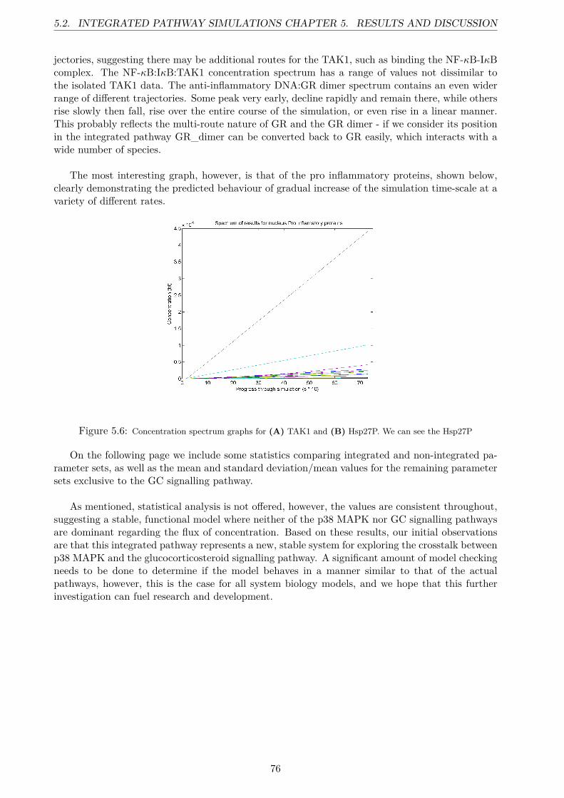
5.2. INTEGRATED PATHWAY SIMULATIONS CHAPTER 5. RESULTS AND DISCUSSION

jectories, suggesting there may be additional routes for the TAK1, such as binding the NF-κB-IκBcomplex. The NF-κB:IκB:TAK1 concentration spectrum has a range of values not dissimilar tothe isolated TAK1 data. The anti-inflammatory DNA:GR dimer spectrum contains an even widerrange of different trajectories. Some peak very early, decline rapidly and remain there, while othersrise slowly then fall, rise over the entire course of the simulation, or even rise in a linear manner.This probably reflects the multi-route nature of GR and the GR dimer - if we consider its positionin the integrated pathway GR_dimer can be converted back to GR easily, which interacts with awide number of species.

The most interesting graph, however, is that of the pro inflammatory proteins, shown below,clearly demonstrating the predicted behaviour of gradual increase of the simulation time-scale at avariety of different rates.

Figure 5.6: Concentration spectrum graphs for (A) TAK1 and (B) Hsp27P. We can see the Hsp27P

On the following page we include some statistics comparing integrated and non-integrated pa-rameter sets, as well as the mean and standard deviation/mean values for the remaining parametersets exclusive to the GC signalling pathway.

As mentioned, statistical analysis is not offered, however, the values are consistent throughout,suggesting a stable, functional model where neither of the p38 MAPK nor GC signalling pathwaysare dominant regarding the flux of concentration. Based on these results, our initial observationsare that this integrated pathway represents a new, stable system for exploring the crosstalk betweenp38 MAPK and the glucocorticosteroid signalling pathway. A significant amount of model checkingneeds to be done to determine if the model behaves in a manner similar to that of the actualpathways, however, this is the case for all system biology models, and we hope that this furtherinvestigation can fuel research and development.

76

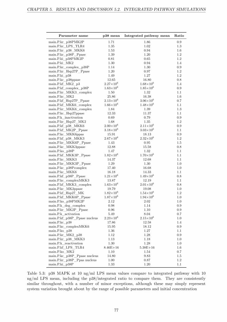
CHAPTER 5. RESULTS AND DISCUSSION 5.2. INTEGRATED PATHWAY SIMULATIONS

Parameter name p38 mean Integrated pathway mean Ratio

main.P.kr_p38PMK2P 1.71 1.86 0.9main.P.kr_LPS_TLR4 1.35 1.02 1.3main.P.kr_p38_MKK6 1.53 0.94 1.6main.P.kr_p38P_Ppase 1.39 1.20 1.2main.P.ki_p38PMK2P 0.81 0.65 1.2main.P.ki_MK2 1.30 0.94 1.4main.P.kr_complex_p38P 1.14 1.30 0.9main.P.kr_Hsp27P_Ppase 1.20 0.97 1.2main.P.ki_p38 1.49 1.27 1.2main.P.kc_p38ppase 12.65 16.80 0.8main.P.kf_MK2_p3 2.27×106 1.68×106 1.4main.P.kf_complex_p38P 1.63×106 1.85×106 0.9main.P.kr_MKK3_complex 1.50 1.32 1.1main.P.kc_MK2 25.86 16.38 1.6main.P.kf_Hsp27P_Ppase 2.13×106 3.06×106 0.7main.P.kf_MKK6_complex 1.66×106 1.48×106 1.1main.P.kr_MKK6_complex 1.84 1.39 1.3main.P.kc_Hsp27ppase 12.33 11.37 1.1main.P.k_inactivation 0.69 0.79 0.9main.P.kr_Hsp27_MK2 1.68 1.35 1.2main.P.kf_p38_MKK6 2.00×106 2.11×106 0.9main.P.kf_MK2P_Ppase 3.18×106 3.03×106 1.1main.P.kc_MKK6ppas 15.91 18.13 0.9main.P.kf_p38_MKK3 2.67×106 2.32×106 1.2main.P.kr_MKK6P_Ppase 1.43 0.95 1.5main.P.kc_MKK3ppase 12.88 15.58 0.8main.P.ko_p38P 1.47 1.32 1.1main.P.kf_MKK3P_Ppase 1.82×106 1.70×106 1.1main.P.kc_MKK3 14.37 12.68 1.1main.P.kr_MKK3P_Ppase 1.29 1.30 1.0main.P.kc_p38Pcomplex 17.40 16.68 1.0main.P.kc_MKK6 16.18 14.33 1.1main.P.kf_p38P_Ppase 1.21×106 1.49×106 0.8main.P.kc_complexMKK3 13.87 12.19 1.1main.P.kf_MKK3_complex 1.63×106 2.01×106 0.8main.P.kc_MK2ppase 19.79 19.08 1.0main.P.kf_Hsp27_MK 1.82×106 1.54×106 1.2main.P.kf_MKK6P_Ppase 1.87×106 1.94×106 1.0main.P.ko_p38PMK2P 2.12 2.02 1.0main.P.k_deg_complex 0.98 1.14 0.9main.P.kr_MK2P_Ppase 0.96 1.10 0.9main.P.k_activation 5.49 8.04 0.7main.P.kf_p38P_Ppase nucleus 2.23×106 2.15×106 1.0main.P.kc_p38 17.86 12.58 1.4main.P.kc_complexMKK6 15.95 18.12 0.9main.P.ko_p38 1.36 1.27 1.1main.P.kr_MK2_p38 1.12 1.28 0.9main.P.kr_p38_MKK3 1.13 1.18 1.0main.P.k_reactivation 1.30 1.28 1.0main.P.kf_LPS_TLR4 8.46E+16 5.38E+16 1.6main.P.ko_MK2 1.10 1.54 0.7main.P.kc_p38P_Ppase nucleus 14.80 9.83 1.5main.P.kr_p38P_Ppas nucleus 1.00 0.87 1.2main.P.ki_p38P 1.33 1.20 1.1

Table 5.3: p38 MAPK at 10 ng/ml LPS mean values compare to integrated pathway with 10ng/ml LPS mean, including the p38/integrated ratio to compare them. They are consistentlysimilar throughout, with a number of minor exceptions, although these may simply representsystem variation brought about by the range of possible parameters and initial concentration

77

5.2. INTEGRATED PATHWAY SIMULATIONS CHAPTER 5. RESULTS AND DISCUSSION

Parameter name p38 stdev/mean Integrated pathway stdev/mean

main.P.kr_p38PMK2P 1.73 1.57main.P.kr_LPS_TLR4 1.99 2.18main.P.kr_p38_MKK6 1.63 2.33main.P.kr_p38P_Ppase 1.95 1.90main.P.ki_p38PMK2P 2.43 2.55main.P.ki_MK2 2.01 2.20main.P.kr_complex_p38P 2.05 1.97main.P.kr_Hsp27P_Ppase 2.17 2.26main.P.ki_p38 1.74 1.86main.P.kc_p38ppase 1.93 1.70main.P.kf_MK2_p3 1.34 1.49main.P.kf_complex_p38P 1.63 1.57main.P.kr_MKK3_complex 1.75 1.94main.P.kc_MK2 1.24 1.51main.P.kf_Hsp27P_Ppase 1.38 1.08main.P.kf_MKK6_complex 1.56 1.64main.P.kr_MKK6_complex 1.66 1.87main.P.kc_Hsp27ppase 1.88 1.98main.P.k_inactivation 2.63 2.56main.P.kr_Hsp27_MK2 1.79 1.86main.P.kf_p38_MKK6 1.46 1.40main.P.kf_MK2P_Ppase 1.05 1.05main.P.kc_MKK6ppas 1.72 1.65main.P.kf_p38_MKK3 1.26 1.29main.P.kr_MKK6P_Ppase 1.77 2.16main.P.kc_MKK3ppase 1.81 1.75main.P.ko_p38P 1.82 1.99main.P.kf_MKK3P_Ppase 1.65 1.60main.P.kc_MKK3 1.93 1.85main.P.kr_MKK3P_Ppase 1.91 1.95main.P.kc_p38Pcomplex 1.69 1.67main.P.kc_MKK6 1.65 1.72main.P.kf_p38P_Ppase 1.83 1.63main.P.kc_complexMKK3 1.87 1.93main.P.kf_MKK3_complex 1.47 1.42main.P.kc_MK2ppase 1.57 1.56main.P.kf_Hsp27_MK 1.49 1.66main.P.kf_MKK6P_Ppase 1.41 1.44main.P.ko_p38PMK2P 1.41 1.46main.P.k_deg_complex 2.30 2.11main.P.kr_MK2P_Ppase 2.43 2.03main.P.k_activation 2.81 2.69main.P.kf_p38P_Ppase nucleus 1.35 1.36main.P.kc_p38 1.73 1.95main.P.kc_complexMKK6 1.65 1.52main.P.ko_p38 1.91 1.97main.P.kr_MK2_p38 2.18 2.06main.P.kr_p38_MKK3 2.16 1.92main.P.k_reactivation 2.03 2.00main.P.kf_LPS_TLR4 2.52 3.15main.P.ko_MK2 2.06 1.73main.P.kc_p38P_Ppase nucleus 1.77 2.12main.P.kr_p38P_Ppas nucleus 2.28 2.38main.P.ki_p38P 2.06 2.07

Table 5.4: Comparing the spread around the mean for 10 ng/ml LPS p38 MAPK pathway andintegrated pathway. Shows a highly similar set of values, indicating the range around the mean iscomparable. This indicates that the integrated pathway is not destabilizing any of the original p38MAPK parameters significantly, adding weight to the idea that it is a stable model.

78

CHAPTER 5. RESULTS AND DISCUSSION 5.2. INTEGRATED PATHWAY SIMULATIONS

Parameter name MEAN STDEV STDEV/Mean

GR\_inactive:GC association rate 2.11×106 2.87×106 1.36GR\_inactive:GC dissociation rate 1.15 2.41 2.09GR:p38P association rate 1.71×106 2.69×106 1.57GR:p38P dissociation rate 1.17 2.45 2.10p38P catalytic rate on GR 13.17 25.70 1.95GR dimerisation rate 1.9×106 2.80×106 1.48GR un-dimerisation rate 1.35 2.74 2.03JNK activation rate 1.29 2.48 1.92JNK inactivation rate 1.44 2.70 1.87JNK:AP1 association rate 1.86×106 2.75×106 1.48JNK:AP1 dissociation rate 1.01 2.20 2.17JNK catalytic rate on AP1 12.92 25.25 1.96AP1P:GR association rate 2.08×106 3.02×106 1.45AP1P:GR dissociation rate 1.28 2.41 1.88NfkB:IkB association rate 1.77×106 2.53×106 1.43NfkB:IkB dissociation rate 0.72 1.72 2.39TAK1:NFkB\_IkB association rate 2.24×106 3.08×106 1.37TAK1:NFkB\_IkB dissociation rate 1.22 2.46 2.01TAK1 catalytic rate on NfkB\_IkB 11.57 24.16 2.09Spontaneous GRP dephosphorylation 1.08 2.22 2.05Spontaneous AP1P dephosphorylation 1.22 2.57 2.11NfkB:GR association rate 2.03×106 2.90×106 1.43NfkB:GR dissociation rate 1.41 2.46 1.75GR dimer nuclear import rate 0.99 2.10 2.11GR dimer nuclear export rate 0.84 2.09 2.48NfkB nuclear import rate 0.97 2.45 2.52NfkB nuclear export rate 1.22 2.32 1.91AP1P nuclear import rate 1.41 2.47 1.75AP1P nuclear export rate 1.24 2.43 1.96GR dimer:antiInf DNA association rate 2.27×1010 3.04×1010 1.34GR dimer:antiInf DNA dissociation rate 0.01 0.02 1.93MKP-1 protein expression rate 0.20 0.31 1.58IkB protein expression rate 0.15 0.28 1.81Nf-kB:proInf DNA association rate 1.80×1010 2.79×1010 1.55Nf-kB:proInf DNA dissociation rate 0.01 0.03 1.95AP1P:proInf DNA association rate 2.55×1010 3.33×1010 1.31AP1P:proInf DNA dissociation rate 0.02 0.03 1.69Pro Inf. DNA:GR dimer association 1.96×1010 2.64×1010 1.35Pro Inf. DNA:GR dimer dissociation 0.01 0.02 2.48Pro inf. protein expression1 rate 0.25 0.33 1.28Pro inf. protein expression2 rate 0.15 0.27 1.80IkB nuclear import rate 0.87 2.04 2.34IkB nuclear export rate 1.66 2.99 1.80

Table 5.5: Final parameter statistics for those constants not additionally in the p38 MAPK pathway.Means and standard deviation/mean are generally consistent with previous values

79

Chapter 6

Conclusion and Further Work

In this final chapter, we overview the project’s progress and achievements, both in a quantitativeand qualitative sense. We then go on to outline the future work regarding the various elements ofthis project, considering both possible avenues of interests and ones being actively explored.

6.1 Project Summary

The initial motivation for this project was to develop a platform from which research into potentialcrosstalk between the glucocorticosteroid (GC) signalling pathway and p38 MAPK could proceed inthe context of corticosteroid resistant (CSR) asthma. CSR asthma represents a significant portionof the cost and mortality associated with the disease, but affects only a tiny fraction of sufferers.By better understanding the molecular mechanism(s) and pathways causing this disease, not onlymay more effective treatments present themselves, but a better understanding of asthma as a wholemay be obtained.

We began with a thorough overview of both possible simulation techniques and the signallingpathways associated with asthma. Included in this early stage work is a three and a half thousandword review of the state of the art regarding BIO-PEPA, included in the electronic submission ofthis project, although not as part of this dissertation. Based on this research, it was decided that,based on current software functionality and availability, BIO-PEPA did not represent an ideal ap-proach to modelling complex signalling pathways. However, being able to fully justify this positionwas very useful, especially in the context of Barkouhk’s dissertation [8].

With a good overview of the signalling processes involved, we began working with an existingsignalling model developed by Hendriks et al. [30] of the p38 MAPK pathway. This pathway isinvolved in the pro inflammatory response, and a number of it’s components are significantly up-regulated in CSR patients. While this model had already been developed, we had to reconstructit into a format usable by matlab before simulations to confirm it’s stability and reliability couldproceed. While this was being carried out, we identified the GC signalling pathway as an idealsystem to combine with the p38 MAPK pathway to investigate possible crosstalk. GCs are usedas the typical treatment for asthma, although CSR patients frequently display insensitivity and upregulated p38 MAPK components. By looking at how these two pathways interact we may be ableto identify putative drug targets at non-traditional locations in the pathway(s).

After an exhaustive literature review, we developed a GC signalling pathway model comparablein design, structure, size, and parameter ranges to the existing p38 MAPK pathway. During thisprocess, it became clear that while developing the GC signalling pathway model as an indepen-dent system was necessary, integrating the two models together by hand was non-trivial. Withthis in mind, we identified a significant lack of existing software to integrate two SBML modelstogether, and so set about the process of developing a complete, generic software tool to achievejust that. After identifying specification goals we used a high velocity scrum style methodology

80

CHAPTER 6. CONCLUSION AND FURTHER WORK 6.2. FUTURE WORK

to develop what ended up being a significant product to integrate two basic SBML1 models together.

With both our p38 MAPK and GC models fully developed, we designed and implemented aset of matlab scripts to carry out a Monte Carlo based parameter generation, simulation andevaluation process on these models. Using pre-existing experimental data as the benchmark, werandomly generate a parameter set, ran the simulation using that parameter set and then evalu-ate how comparable the simulation outcome was with the previously reported experimental data.Initially the p38 MAPK model was used (which we had previously tested using the best fittingidealized parameter set presented by Hendriks et al.) to generate 388 parameter sets with a coef-ficient comparison between normalized experimental/simulation generated data of 0.88 (the bestfitting Hendriks parameter set was around 0.6 when normalized). When the project began, itwas envisaged that by working in parallel with Prof. Ian Adcock we would obtain empirical datarelating to experimental conditions relevant to the integrated pathway, which we could then useto generate an evaluation function to identify operational parameter sets for the integrated modelin the same way as we had shown for the p38 MAPK model. Unfortunately this data was notavailable, however, we were able to generate some entirely synthetic data and use the p38 MAPKexperimental data to evaluate that our integrated model was functional and produced plausibleoutput, even if the actual data was not biologically relevant. With this successfully done, the workrequired to generate correctly evaluated parameters for the integrated pathway is simply a case ofentering in the new empirical data running the scripts.

6.2 Future WorkAs mentioned in the preceding section, this project comprises of related yet independent compo-nents;

• Reconstruction of the p38 MAPK pathway model, originally developed by Hendriks et al [30]into a more efficient, syntactically correct matlab compliant SBML model

• A totally novel SBML implementation of the GC signalling pathway based on a significantamount of data and good understanding of the underlying biochemical processes

• A software tool for integrating two SBML models together in a semantically and syntacticallycorrect manner

• A set of matlab scripts for automating the process of generating random parameters, runninga simulation with those parameters, assessing if the generated model meets the experimentalcriterion and then either discarding or saving the parameter sets

We consider each of these four elements in turn, evaluating future endeavours, as well as finallyconsidering the extension of this project.

6.2.1 p38 MAPK Model

While semantically this model was already in the public domain, it was in a not easily usableformat. Despite being described as SBML, the original file failed to comply to either SBML ormatlab specifications for model manipulation. We do not presume to suggest that without thiswork further development and work based on this model would not have been possible, however,it significantly reduces the friction associated with justifying future projects using the model. Thep38 MAPK pathway is central to a significant number of biological process, and is especiallyrelevant in the prognosis and diagnosis of cancer[17]. With our SBMLIntegrator software, havingan operational and widely available version of the MAPK model may facilitate future investigation

1Basic here denotes a model which contains one or more of the SBML elements: Unit Definition, Compartment,Species, Parameter, Rule or Reaction

81

6.3. FINAL PROJECT WORK CHAPTER 6. CONCLUSION AND FURTHER WORK

into cancer-related signalling. We plan to discuss the possible submission of this updated versionto the BioModels database with Hendriks et al.

6.2.2 Glucocorticosteriod Signalling Pathway

To our knowledge there are no GC signalling models which convey the detail of ours. Additionally,our approach of modelling gene expression has not been seen in any other SBML models either.Clearly a great deal of additional work needs to be done to verify that this model and the integrationmodel are valid, but using SBMLIntegrator we can easily make changes to the seperate GC signallingpathway and re-integrate the two. It is hoped that when the empirical data produced by Prof.Adcock becomes available we will be able to begin a significant and more advanced parameterestimation process on the integrated pathway. Based on the results if these simulations, the presenceof pathway crosstalk should be easily identifiable. It is important to remember that crosstalk inthis model does not necessarily mean that biological models participate in crosstalk. However, itmay indicate potential future experimental targets, which could confirm or deny it’s existence.

6.2.3 SBMLIntegrator

The SBMLIntegrator software is currently available through github 2 and is in it’s alpha stageof public release. Over the next few weeks we will add in additional functionality relating tothe SBML elements not already covered by the implementation (function definitions, constraints,initial assignments and events). In addition, we are in the process of discussing with the SBMLcommunity features for a good, fast GUI based model designer and integrator3. By gauging specificdesires of those who use the software most, we will attempt to use the underlying SBMLIntegratorcore to construct an SBML modelling tool. There is discussion with other developers around theworld regarding pooling resources, and we hope to have a functional version of this software upand running my mid October.

6.2.4 Parameter Generation and Evaluation

Our matlab tools for parameter estimation have provided an efficient, fast and effective way togenerate a widely ranging set of parameters for our model estimation. However, there are issuesassociated with the number distribution of the random values generated, but with the rangesprovided a uniformly distributed random number creates such a vast search space that a simple,Monte-Carlo approach is not tractable for a system of this size. We would suggest, therefore, thatthe development of intelligent parameter estimation algorithms represents a significant challengefacing not only this project, but the entire parameter estimation space. Using a guided Monte Carloapproach may facilitate favourable results, whereby a search space is narrowed based on a dynamicprogramming approach in a top down manner. Such an algorithm would have a significant impacton the systems biology discipline as a whole, and could allow for automated parameter estimationfor models on the BioModels database.

6.3 Final Project WorkAs a final note, work has begun on a paper detailing the results of this project. We focus on thedevelopment of the glucocorticosteriod model and it’s integration with the p38 MAPK model. Ifthe empirical data becomes available during this write up process it may be possible to incorporatesome of the results and analysis here. However, irrespectively, it will provide an example of thedevelopment of an associated signalling pathway based on an existing one, and the progress ofdeveloping a system where the pathway interface can be explored. We hope that by providingthe tools to carry out this integration that there will be an increase in the research into signallingcrosstalk, an area where systems biology has the potential to yield great results.

2https://github.com/rednaxela/SBMLIntegrator3http://sbml.org/Forums/index.php?t=msg&goto=7160&rid=6678#msg_7160

82

Appendix A

SBMLIntegrator

A.1 SBMLIntegrator Output Screens

A.1.1 Explore Model

---------------------------------------NB: ModelSelect components to show---------------------------------------[1] ------------ Function Definitions[2] ------------ Unit Definitions[3] ------------ Compartments[4] ------------ Species[5] ------------ Parameters[6] ------------ Rules[7] ------------ Initial Assignments[8] ------------ Constraints[9] ------------ Reactions[10] ----------- Events[11] ----------- ReturnSelect:

Interface 11: Explore model initial screen - from here each option goves a list of the various elementsand their attributes. If a value is abscent from an attribute we display the fact with message

83

A.1. SBMLINTEGRATOR OUTPUT SCREENS APPENDIX A. SBMLINTEGRATOR

A.1.2 Display Summary

################################################################################### Display Summary ##################################################################################File name ---------------- p38model.xmlModel ID -----------------Model name ---------------Model version ------------ 1ModeL level -------------- 2Model substance units ----Model time units ---------Model volume units -------Model area units ---------Model length units -------Model extent units -------Model conversion factor -----------------------------------Summary of model components---------------------------------No of funtions ----------- 0No of unit definitions --- 19No of compartments ------- 4No of species ------------ 40No of parameters --------- 169No of initial assigments - 0No of rules -------------- 101No of constraints -------- 0No of reactions ---------- 35No of events ------------- 0----------------------------------

Interface 12: Model summary screen, with the original p38-MAPK model as the example

84

APPENDIX A. SBMLINTEGRATOR A.1. SBMLINTEGRATOR OUTPUT SCREENS

A.1.3 Display Compartments

################################################################################# Display Compartments ###############################################################################There are 4 compartments defined;Compartment [1] ID(main_cytosol) name(cytosol)

Spatial Dimensions: 3Size: 1Units: litreConstant: 1

Compartment [2] ID(main_Medium) name(Medium)Spatial Dimensions: 3Size: 1Units: litreConstant: 1

Interface 13: Compartment viewer, describing the two of the compartments in the original p38MAPK model

A.1.4 Display Reactions

################################################################################### Display Reaction #################################################################################There are 35 reactions defined;Reaction [1] Name(Rxn1271) ID(main_cytosol_Rxn1271)

main_cytosol_complex_MKK6 <---> main_cytosol_complex + main_cytosol_MKK6P

Modfiers: <none>Rate law: main_cytosol_Rxn1271_Flux

Local parameters: 0Global parameters: 0Referenced rule: main_cytosol_Rxn1271_Kf * main_cytosol_complex_MKK6* main_cytosol

Interface 14: Reaction viewer, describing the one of the reactions in the original p38 MAPK model

85

A.1. SBMLINTEGRATOR OUTPUT SCREENS APPENDIX A. SBMLINTEGRATOR

A.1.5 Display Rules

#################################################################################### Display Rules ###################################################################################There are 101 rules defined;Rule [1] ID(main_cytosol_Rxn1534_Kf)

Assignment rule: main_P_kf_LPS_TLR4 * main_cytosolUnits: litre^(2) * second^(-1) * mole^(-1)

Rule [2] ID(main_cytosol_Rxn126_Kr)Assignment rule: main_P_kr_p38P_PpaseUnits: second^(-1)

Rule [3] ID(main_nucleus_Rxn1_Kr)Assignment rule: main_P_kr_MK2_p38Units: second^(-1)

Interface 15: Rules viewer, describing three of the rules in the original p38 MAPK model

86

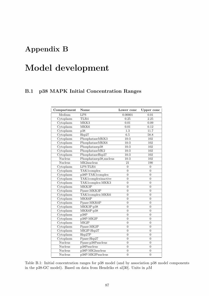
Appendix B

Model development

B.1 p38 MAPK Initial Concentration Ranges

Compartment Name Lower conc Upper concMedium LPS 0.00001 0.01

Cytoplasm TLR4 0.25 2.25Cytoplasm MKK3 0.01 0.09Cytoplasm MKK6 0.01 0.12Cytoplasm p38 1.3 11.7Cytoplasm Hsp27 6.5 58.8Cytoplasm PhosphataseMKK3 10-3 102Cytoplasm PhosphataseMKK6 10-3 102Cytoplasm Phosphatasep38 10-3 102Cytoplasm PhosphataseMK2 10-3 102Cytoplasm PhosphataseHsp27 10-3 102Nucleus Phosphatasep38,nucleus 10-3 102Nucleus MK2nucleus 21 190

Cytoplasm LPS:TLR4 0 0Cytoplasm TAK1complex 0 0Cytoplasm p38P:TAK1complex 0 0Cytoplasm TAK1complexinactive 0 0Cytoplasm TAK1complex:MKK3 0 0Cytoplasm MKK3P 0 0Cytoplasm Ppase:MKK3P 0 0Cytoplasm TAK1complex:MKK6 0 0Cytoplasm MKK6P 0 0Cytoplasm Ppase:MKK6P 0 0Cytoplasm MKK3P:p38 0 0Cytoplasm MKK6P:p38 0 0Cytoplasm p38P 0 0Cytoplasm p38P:MK2P 0 0Cytoplasm MK2P 0 0Cytoplasm Ppase:MK2P 0 0Cytoplasm MK2P:Hsp27 0 0Cytoplasm Hsp27P 0 0Cytoplasm Ppase:Hsp27 0 0Nucleus Ppase:p38Pnucleus 0 0Nucleus p38Pnucleus 0 0Nucleus p38P:MK2nucleus 0 0Nucleus p38P:MK2Pnucleus 0 0

Table B.1: Initial concentration ranges for p38 model (and by association p38 model componentsin the p38-GC model). Based on data from Hendriks et al[30]. Units in µM

87

B.2. P38 MAPK PARAMETER RANGES APPENDIX B. MODEL DEVELOPMENT

B.2 p38 MAPK Parameter Ranges

Name Description Rxn Lower Upper UnitsV olumecytosol Cytosolic volume 10−12 10−12 Lvolumenucleus Nuclear volume 10−13 10−13 Lkf,LP S:T LR4 LPS:TLR4 association rate 1 107 1018 M−1 min−1

kr,LP S:T LR4 LPS:TLR4 dissociation rate 1 10−4 101 min−1

kactivation LPS:TLR4 -> TAK1complex activation rate 2 10−4 102 min−1

kdeactivation TAK1complex deactivation rate 2 10−4 101 min−1

kreactivation TAK1complexinactive reactivation rate 4 10−4 101 min−1

kdeg,complex TAK1complex degradation rate 3 10−4 101 min−1

kf,complex:p38P TAK1complex:phospho-p38 association rate 5 104 107 M−1 min−1

kr,complex:p38P TAK1complex:phospho-p38 dissociation rate 5 10−4 101 min−1

kc,p38P :complex phospho-p38 catalytic rate for TAK1complex 6 10−2 102 min−1

kf,MKK3:complex TAK1complex:MKK3 association rate 11 104 107 M−1 min−1

kr,MKK3:complex TAK1complex:MKK3 dissociation rate 11 10−4 101 min−1

kc,complex(MKK3) TAK1complex catalytic rate for MKK3 12 10−2 102 min−1

kf,MKK3P :P pase phospho-MKK3:PhosphataseMKK3 association rate 14 104 107 M−1 min−1

kr,MKK3:P pase phospho-MKK3:PhosphataseMKK3 dissociation rate 14 10−4 101 min−1

kc,P paseMKK3 PhosphataseMKK3 catalytic rate 13 10−2 102 min−1

kf,MKK6:complex TAK1complex:MKK6 association rate 7 104 107 M−1 min−1

kr,MKK6;complex TAK1complex:MKK6 dissociation rate 7 10−4 101 min−1

kc,complex(MKK6) TAK1complex catalytic rate for MKK6 8 10−2 102 min−1

kf,MKK6P :P pase phospho-MKK6:PhosphataseMKK6 association rate 10 104 107 M−1 min−1

kr,MKK6P :P pase phospho-MKK6:PhosphataseMKK6 dissociation rate 10 10−4 101 min−1

kc,P paseMKK6 PhosphataseMKK6 catalytic rate 9 10−2 102 min−1

kf,p38:MKK3 phospho-MKK3:p38 association rate 15 104 107 M−1 min−1

kr,p38:MKK3 phospho-MKK3:p38 dissociation rate 15 10−4 101 min−1

kc,MKK3 phospho-MKK3 catalytic rate 16 10−2 102 min−1

kf,p38:MKK6 phospho-MKK6:p38 association rate 17 104 107 M−1 min−1

kr,p38:MKK6 phospho-MKK6:p38 dissociation rate 17 10−4 101 min−1

kc,MKK6 phospho-MKK6 catalytic rate 18 10−2 102 min−1

kf,p38P :P pase phospho-p38:Phosphatasep38 association rate (cytosol) 20 104 107 M−1 min−1

kr,p38P :P pase phospho-p38:Phosphatasep38p38 dissociation rate (cytosol) 20 10−4 101 min−1

kc,P pasep38 Phosphatasepp38 catalytic rate (cytosol) 19 10−2 102 min−1

kf,p38P :P pase,nucleus phospho-p38:Phosphatasep38 association rate (nucleus) 21 104 107 M−1 min−1

kr,p38P :P pase,nucleus phospho-p38:Phosphatasep38 dissociation rate (nucleus) 21 10−4 101 min−1

kc,p38P :P pase,nucleus Phosphatasep38 catalytic rate (nucleus) 22 10−2 102 min−1

kf,MK2:p38 phospho-p38:MK2 association rate 23 104 107 M−1 min−1

kr,MK2:p38 phospho-p38:MK2 dissociation rate 23 10−4 101 min−1

kc,p38 phospho-p38 catalytic rate for MK2 24 10−2 102 min−1

kr,p38P :MK2P phospho-p38:phospho-MK2 dissociation rate 25 10−4 101 min−1

kf,MK2P :P pase phospho-MK2:PhosphataseMK2 association rate 26 104 107 M−1 min−1

kr,MK2P :P pase phospho-MK2:PhosphataseMK2 dissociation rate 26 10−4 101 min−1

kc,P paseMK2 PhosphataseMK2 catalytic rate 27 10−2 102 min−1

kf,Hsp27:MK2 phospho-MK2:Hsp27 association rate 28 104 107 M−1 min−1

kr,Hsp27:MK2 phospho-MK2:Hsp27 dissociation rate 28 10−4 101 min−1

kc,MK2 phospho-MK2 catalytic rate 29 10−2 102 min−1

kf,Hsp27P :P pase phospho-Hsp27:PhosphataseHsp27 association rate 30 104 107 M−1 min−1

kr,Hsp27P :P pase phospho-Hsp27:PhosphataseHsp27 dissociation rate 30 10−4 101 min−1

kc,P paseHsp27 PhosphataseHsp27 catalytic rate 31 10−2 102 min−1

ki,p38 p38 nuclear import rate 32 10−4 101 min−1

ko,p38 p38 nuclear export rate 32 10−4 101 min−1

ki,p38P phospho-p38 nuclear import rate 33 10−4 101 min−1

ko,p38P phospho-p38 nuclear export rate 33 10−4 101 min−1

ki,p38P :MK2P phospho-p38:phospho-MK2 nuclear co-import rate 34 10−4 101 min−1

ko,p38P :MK2P phospho-p38:phospho-MK2 nuclear co-export rate 34 10−4 101 min−1

ki,MK2 MK2 nuclear import rate 35 10−4 101 min−1

ko,MK2 MK2 nuclear export rate 35 10−4 101 min−1

Table B.2: p38 MAPK parameter ranges

88

Appendix C

Simulation results

Figure C.1: (A) - Cytosol degradation concentration spectrum graph and (B) - TAK1:MKK3 concentrationspectrum graphs, both at 10ng/ml

Figure C.2: (C) - MKK6 concentration spectrum graph and (D) - MK2_phosphatase concentration spectrumgraphs, both at 10ng/ml

89

APPENDIX C. SIMULATION RESULTS

Figure C.3: (E) - p38P:TAK1 concentration spectrum graph and (F) - LPS:TLR4 concentration spectrum graphs,both at 10ng/ml

Figure C.4: (G) - MK2P concentration spectrum graph and (H) - Nuclear localized p38P:MK2concentrationspectrum graphs, both at 10ng/ml

90

Acronyms

AP-1 Activator Protein-1. 20

CDK Cylcin Dependent Kinase. 21

CSR Corticosteroid Resistant. 4, 21, 22, 79

CTMC Continous Time Markov Chain. 11–13

DNA Deoxyribonucleic Acid. 6

ERK Extracellular Regulated Kinase. 20

GC Glucocorticosteroid. 4, 5, 19, 22, 25, 51, 59, 60, 62, 63, 68, 74, 75, 79–81

GR Glucocortocoid Receptors. 20, 22, 54, 62

GRE Glucocortocoid Response Element. 20

GSK-3 Glycogen Synthase Kinase 3. 21

hsp Heat Shock Protein. 20

IL Interleukin. 19

IL-13 Interleukin-13. 51

IL-2 Interleukin-2. 51

IL-4 Interleukin-4. 51

IRI Import Replace Integrate. 29, 41

JNK c-Jun N-terminal Kinase. 20, 21

LABAs Long Acting β Agonists. 19

MAPK Mitogen Activated Protein Kinase. 20, 21

MCA Metabolic Control Analysis. 6

MKP-1 MAPK phosphatase-1. 20

mRNA Messenger Ribonucleic Acid. 8

MWC Monod Wyman Changeux. 11

ODEs Ordinary Differential Equations. 12

91

Acronyms Acronyms

PBMCs Peripheral Blood Mononuclear Cells. 21

PPI Protein Protein Interaction. 9

RNA xRibonucleic Acid. 6

SBML Systems Biology Markup Language. 4, 16

SPA Stochastic Process Algebra. 11

TNF Tumour Necrosis Factor. 19

XML Extensible Markup Language. 16

92

Bibliography

[1] Devrim Acehan, Xuejun Jiang, David Gene Morgan, John E Heuser, Xiaodong Wang, andChristopher W Akey. Three-dimensional structure of the apoptosome: Implications for assem-bly, procaspase-9 binding, and activation. Molecular Cell, 9(2):423–432, February 2002.

[2] I M Adcock, S J Lane, C R Brown, T H Lee, and P J Barnes. Abnormal glucocorticoid receptor-activator protein 1 interaction in steroid-resistant asthma. The Journal of ExperimentalMedicine, 182(6):1951–1958, December 1995.

[3] Ian M. Adcock and Peter J. Barnes. Molecular mechanisms of corticosteroid resistance.CHEST, 134-2:394–401, 2008.

[4] Ian M Adcock and Gaetano Caramori. Cross-talk between pro-inflammatory transcriptionfactors and glucocorticoids. Immunol Cell Biol, 79(4):376–384, August 2001.

[5] A.S. Baldwin Jr. Series introduction: the transcription factor nf-kappab and human disease.J Clin Invest, 107:3–6, 2001.

[6] Peter Barnes and Michael Karin. Nuclear factor-kb: a pivotal transcription factor in chronicinflammatory diseases. The New England journal of medicine, 336 : 15:1066, 1997.

[7] Peter J. Barnes. Efficacy of inhaled corticosteroids in asthma. Journal of Allergy and ClinicalImmunology, 102(4):531–538, October 1998.

[8] C. Baroukh. Representing biological processes using process calculus. Master’s thesis, ImperialCollege London, 2010.

[9] Falko Baus and Pieter S Kritzinge. Stochastic Petri Nets - An Introduction to the Theory.Bause and Kritzinger, 2002.

[10] P. Bhavsar, N. Khorasani, M. Hew, M. Johnson, and K. F. Chung. Effect of p38 mapk inhibi-tion on corticosteroid suppression of cytokine release in severe asthma. European RespiratoryJournal, 35(4):750–756, April 2010.

[11] Falk Schreiber Björn H. Junker. Analysis of Biological Networks. Wiley, 2008.

[12] Corren J Bensch G Busse WW Whitmore J Borish LC, Nelson HS. Efficacy of soluble il-4receptor for the treatment of adults with asthma. J Allergy Clin Immunol, 107:963–970, 2001.

[13] Tim Bray, Jean Paoli, C. M. Sperberg-McQueen, Eve Maler, and François Yergeau. Extensiblemarkup language (xml) 1.0 (fifth edition), November 2008.

[14] Matthew D. Brown and David B. Sacks. Protein scaffolds in map kinase signalling. CellularSignalling, 21(4):462–469, April 2009.

[15] M Brunner and H. Bujard. Promoter recognition and promoter strength in the escherichia colisystem. EMBO J, 6(10):3139–3144, 1987.

[16] Federica Ciocchetta and Jane Hillston. Bio-pepa: An extension of the process algebra pepafor biochemical networks. Electron. Notes Theor. Comput. Sci, 194:3:103–117, 2008.

93

BIBLIOGRAPHY BIBLIOGRAPHY

[17] A S Dhillon, S Hagan, O Rath, and W Kolch. Map kinase signalling pathways in cancer.Oncogene, 26(22):3279–3290, 0000.

[18] Danielle Duma, Christine M. Jewell, and John A. Cidlowski. Multiple glucocorticoid re-ceptor isoforms and mechanisms of post-translational modification. The Journal of SteroidBiochemistry and Molecular Biology, 102(1-5):11–21, December 2006.

[19] R Duncan and EH McConkey. How many proteins are there in a typical mammalian cell?Clin Chem, 28(4):749–755, April 1982.

[20] T. Kino E. Charmandari. Novel causes of generalized glucocorticoid resistance. Horm MetabRes, 39(6):445–450, 2007.

[21] Michael R. Edwards, Nathan W. Bartlett, Deborah Clarke, Mark Birrell, Maria Belvisi, andSebastian L. Johnston. Targeting the nf-[kappa]b pathway in asthma and chronic obstructivepulmonary disease. Pharmacology & Therapeutics, 121(1):1–13, January 2009.

[22] D. Fell. Metabolic control analysis: a survey of its theoretical and experimental development.Biochem J., 286 Part-2:313–330, 1992.

[23] D. Gilbert and M. Heiner. From petri nets to differential equations - an integrative approachfor biochemical network analysis. Lecture Notes in Computer Science, 4024:181–200, 2006.

[24] D. Gillespie. Exact stochastic simulation of coupled chemical reactions. J. Phys. Chem,81:2340–2361, 1977.

[25] Daniel T. Gillespie. A general method for numerically simulating the stochastic time evolutionof coupled chemical reactions. Journal of Computational Physics, 22:403, 1976.

[26] Peter J. E. Goss and Jean Peccoud. Quantitative modeling of stochastic systems in molecularbiology by using stochastic petri nets. Proceedings of the National Academy of Sciences,95(12):6750–6755, June 1998.

[27] Maria Luisa Guerriero. Qualitative and quantitative analysis of a bio-pepa model of thegp130/jak/stat signalling pathway. Lecture Notes in Computer Science, 5750:90–115, 2009.

[28] C.M. Guldberg and P. Waage. Uber die chemische affinitat. Journal fur Pracktische Chemie,19:69, 1879.

[29] S Lawrence Zipursky Paul Matsudaira David Baltimore Harvey Lodish, Arnold Berk andJames Darnell. Molecular Cell Biology, 4th edition. New York: W. H. Freeman, 2000. ISBN-10: 0-7167-3136-3.

[30] Bart S. Hendriks, Fei Hua, and Jeffrey R. Chabot. Analysis of mechanistic pathway modelsin drug discovery: p38 pathway. Biotechnology Progress, 24(1):96–109, 2008.

[31] A. V. Hill. The possible effects of the aggregation of the molecules of huemoglobin on itsdissociation curves. Proceedings of the Physilogical Society (Sup), 40:4–7, 1910.

[32] C. A. R. Hoare. Communicating sequential processes. Commun. ACM, 21(8):666–677, 1978.

[33] A. L. Hodgkin and A. F. Huxley. A quantitative description of membrane current and itsapplication to conduction and excitation in nerve. J Physiol., 117(4):500–544, 1952.

[34] Michael Hucka, Frank T. Bergmann, Stefan Hoops, Sarah M. Keating, Sven Sahle, James C.Schaff, Lucian P. Smith, and Darren J. Wilkinson. The systems biology markup lan-guage (sbml): Language specification for level 3 version 1 core. Nature Precedings,http://dx.doi.org/10.1038/npre.2010.4959.1:–, 2010.

94

BIBLIOGRAPHY BIBLIOGRAPHY

[35] Elvis Irusen, John G. Matthews, Atsushi Takahashi, Peter J. Barnes, Kian F. Chung, andIan M. Adcock. p38 mitogen-activated protein kinase-induced glucocorticoid receptor phos-phorylation reduces its activity: Role in steroid-insensitive asthma. Journal of Allergy andClinical Immunology, 109(4):649–657, April 2002.

[36] K. Ito, KF. Chung, and IM. Adcock. Update on glucocorticoid action and resistance. J AllergyClin Immunol, 117:522–543, 2006.

[37] Eric Jacques, Abdelhabib Semlali, Louis-Philippe Boulet, and Jamila Chakir. Ap-1 overex-pression impairs corticosteroid inhibition of collagen production by fibroblasts isolated fromasthmatic subjects. American Journal of Physiology - Lung Cellular and Molecular Physiology,–:–, June 2010.

[38] John L Tymoczko Jeremy M Berg and Lubert Stryer. Biochemistry, 5th edition. New York:W H Freeman, 2002.

[39] H. Kacser and J. A. Burns. The control of flux. Symp Soc Exp Biol., 27:65–104, 1973.

[40] A. D. King, N. Pržulj, and I. Jurisica. Protein complex prediction via cost-based clustering.Bioinformatics, 20(17):3013–3020, November 2004.

[41] Tomoshige Kino, Takamasa Ichijo, Niranjana D. Amin, Sashi Kesavapany, Yonghong Wang,Nancy Kim, Sandesh Rao, Audrey Player, Ya-Li Zheng, Michael J. Garabedian, ErnestKawasaki, Harish C. Pant, and George P. Chrousos. Cyclin-dependent kinase 5 differentiallyregulates the transcriptional activity of the glucocorticoid receptor through phosphorylation:Clinical implications for the nervous system response to glucocorticoids and stress. MolecularEndocrinology, 21(7):1552–1568, July 2007.

[42] J.C. Kips, B.J. O’Connor, S.J. Langley, A. Woodcock, H.A. Kerstjens, and D.S Postma. Effectof sch55700, a humanized anti-human interleukin-5 antibody, in severe persistent asthma: apilot study. Am J Respir Crit Care Med, 167:1655–1659, 2003.

[43] J. Koomey. Why we can expect ever more amazing mobile computing devices in the yearsahead (presentation), 2011.

[44] C. Kuttler and J. Niehren. Gene regulation in the pi calculus: simulating cooperativity at thelambda switch. Transactions on Computational Systems Biology, 4230-VII:24–55, 2004.

[45] SJ Lane, BA Atkinson, R Swaminathan, and TH Lee. Hypothalamic-pituitary-adrenal axisin corticosteroid-resistant bronchial asthma. Am. J. Respir. Crit. Care Med., 153(2):557–560,February 1996.

[46] SJ. Lane, JB Palmer., IF. Skidmore, and TH. Lee. Corticosteroid pharmacokinetics in asthma.Lancet., 17;336(8725):1265, 1990 Nov.

[47] D Y Leung, R J Martin, S J Szefler, E R Sher, S Ying, A B Kay, and Q Hamid. Dysregulation ofinterleukin 4, interleukin 5, and interferon gamma gene expression in steroid-resistant asthma.The Journal of Experimental Medicine, 181(1):33–40, January 1995.

[48] Donald Y. M. Leung and John W Bloom. Update on glucocorticoid action and resistance.Journal of Allergy and Clinical Immunology, 111(1):3–22, January 2003.

[49] Mathworks. Matlab simbiology package, 2011.

[50] L. Menten and M.I. Michaelis. Die kinetik der invertinwirkung. Biochem Z, 49:333–369, 1913.

[51] Aaron L. Miller, M. Scott Webb, Alicja J. Copik, Yongxin Wang, Betty H. Johnson, Raj Ku-mar, and E. Brad Thompson. p38 mitogen-activated protein kinase (mapk) is a key mediatorin glucocorticoid-induced apoptosis of lymphoid cells: Correlation between p38 mapk activa-tion and site-specific phosphorylation of the human glucocorticoid receptor at serine 211. MolEndocrinol, 19(6):1569–1583, June 2005.

95

BIBLIOGRAPHY BIBLIOGRAPHY

[52] Kenneth Murphy. Immunobiology. Garlander Science, 2011.

[53] Brian M. Necela and John A. Cidlowski. Mechanisms of glucocorticoid receptor action innoninflammatory and inflammatory cells. Proc Am Thorac Soc, 1(3):239–246, November2004.

[54] NHLBI. Asthma overview, Feb 2011.

[55] P.M. O’Byrne, M.D. Inman, and E. Adelroth. Reassessing the th2 cytokine basis of asthma.Trends Pharmacol Sci, 25:244–248, 2004.

[56] BioModels Database A Database of Annotated Published Models.http://www.ebi.ac.uk/biomodels-main/.

[57] KEGG: Kyoto Encyclopedia of Genes and Genomes. http://www.genome.jp/kegg/.

[58] Andrea Degasperi Ozgur E. Akman, Federica Ciocchetta and Maria Luisa Guerriero. Mod-elling biological clocks with bio-pepa: Stochasticity and robustness for the neurospora crassacircadian network. Lecture Notes in Computer Science, 5688:52–67, 2009.

[59] Klaus Paal, Patrick A. Baeuerle, and M. Lienhard Schmitz. Basal transcription factors tbpand tfiib and the viral coactivator e1a 13s bind with distinct affinities and kinetics to thetransactivation domain of nf-kb p65. Nucleic Acids Research, 25(5):1050–1055, March 1997.

[60] James C. Phillips, Rosemary Braun, Wei Wang, James Gumbart, Emad Tajkhorshid, ElizabethVilla, Christophe Chipot, Robert D. Skeel, Laxmikant Kalé, and Klaus Schulten. Scalablemolecular dynamics with namd. J. Comput. Chem., 26(16):1781–1802, 2005.

[61] M. Rathinam, L. Petzold, Y. Cao, and D. Gillespie. Stiffness in stochastic chemically reactingsystems: The implicit tau-leaping method. The Journal of Chemical Physics, 119:12784, 2003.

[62] Zoltán Szatmáry, Michael J. Garabedian, and Jan Vilček. Inhibition of glucocorticoid receptor-mediated transcriptional activation by p38 mitogen-activated protein (map) kinase. Journalof Biological Chemistry, 279(42):43708–43715, October 2004.

[63] W. TRAUB, A. YONATH, and D. M. SEGAL. On the molecular structure of collagen. Nature,221(5184):914–917, March 1969.

[64] Fyodor D. Urnov and Alan P. Wolffe. Chromatin remodeling and transcriptional activation:the cast (in order of appearance). Oncogene, 20:2991–3006, 2001.

[65] Dimitri van Heesch. Doxygen - generate documentation from source code(http://www.stack.nl/ dimitri/doxygen/).

[66] Donald Voet and Judith G. Voet. Biochemistry, 4th Edition. Wiley, 2011.

[67] D. C. Walker, J. Southgate, G. Hill, M. Holcombe, D. R. Hose, S. M. Wood, S. Mac Neil, andR. H. Smallwood. The epitheliome: agent-based modelling of the social behaviour of cells.Biosystems, 76(1-3):89–100, August.

[68] Zhen Wang, Weiwei Chen, Evelyn Kono, Thoa Dang, and Michael J. Garabedian. Modula-tion of glucocorticoid receptor phosphorylation and transcriptional activity by a c-terminal-associated protein phosphatase. Molecular Endocrinology, 21(3):625–634, March 2007.

[69] Nancy L. Weigel and Nicole L. Moore. Steroid receptor phosphorylation: A key modulator ofmultiple receptor functions. Molecular Endocrinology, 21(10):2311–2319, October 2007.

[70] Wikipedia. Petri net image, 2011.

[71] Marsha Wills-Karp, Jackie Luyimbazi, Xueying Xu, Brian Schofield, Tamlyn Y. Neben,Christopher L. Karp, and Debra D. Donaldson. Interleukin-13: Central mediator of aller-gic asthma. Science, 282(5397):2258–2261, December 1998.

96