Embed Size (px)
Citation preview

System Modeling and Simulation 06CS82
Dept of ISE,SJBIT Page 1
VTU QUESTION PAPER SOLUTION
June 2012
1. List any three situations when simulation tool is appropriate and not appropriate tool.
6 M
Ans: When Simulation is the Appropriate Tool
Simulation enables the study of and experimentation with the internal interactions of a
complex system, or of a subsystem within a complex system.
Informational, organizational and environmental changes can be simulated and the effect of
those alternations on the model’s behavior can be observer.
The knowledge gained in designing a simulation model can be of great value toward
suggesting improvement in the system under investigation
By changing simulation inputs and observing the resulting outputs, valuable insight may be
obtained into which variables are most important and how variables interact
When Simulation is Not Appropriate
Simulation should be used when the problem cannot be solved using common sense.
Simulation should not be used if the problem can be solved analytically.
Simulation should not be used, if it is easier to perform direct experiments.
Simulation should not be used, if the costs exceeds savings.
b. Define the following terms used in simulation 6 M
Ans: i) discrete system
Systems in which the changes are predominantly discontinuous are called discrete systems. Ex: Bank
– the number of customer’s changes only when a customer arrives or when the service provided a
customer is completed.
ii)continuous system
Systems in which the changes are predominantly smooth are called continuous system. Ex: Head of a
water behind a dam.

System Modeling and Simulation 06CS82
Dept of ISE,SJBIT Page 2
iii) stochastic system
Has one or more random variable as inputs. Random inputs leads to random outputs. Ex: Simulation
of a bank involves random interarrival and service times.
iv)deterministic system
Contains no random variables. They have a known set of inputs which will result in a unique set of
outputs. Ex: Arrival of patients to the Dentist at the scheduled appointment time
v)entity
An entity is an object of interest in a system.
Ex: In the factory system, departments, orders, parts and products are The entities
vi)Attribute
An attribute denotes the property of an entity.
Ex: Quantities for each order, type of part, or number of machines in a Department are attributes of
factory system
c. Draw the flowchart of steps involved in simulation study. 8 M
2a) Consider the grocery store with one check out counter. Prepare the simulation table for
eight customers and find out average waiting time of customer in queue,idle time of server and
average service time .The inter arrival time (IAT) and service time (ST) are given in minutes.

System Modeling and Simulation 06CS82
Dept of ISE,SJBIT Page 3
IAT : 3,2,6,4,4,5,8
ST(min) :3,5,5,8,4,6,2,3
Assume first customer arrives at time t=0 10 M
2b) Suppose the maximum inventory level is M 11 units and the review period is 5 days estimate
by simulation the average ending units in inventory and number of days when a shortage
condition occurs .Initial simulation is started with level of 3 units and an order of 8 units
scheduled to arrive in two days time.Simulate for three cycles (15 days) The probability for daily
demand and lead time is given below 10 M
Demand 0 1 2 3 4
P 0.1 0.25 0.35 0.2 0.1
Lead time 1 2 3
Propability 0.5 0.3 0.2
RD for demand: 24,35,65,25,8,85,77,68,28,5,92,55,49,69,70

System Modeling and Simulation 06CS82
Dept of ISE,SJBIT Page 4
RD for lead time :5,0,3
3a) Define the term used in discrete event simulation: 6M
i) System safe ii)list iii) event iv)FEL v) delay vi)system Ans:
i) System safe
A collection of variables that contain all the information necessary to describe the system at any time
ii) list
A collection of (permanently or temporarily) associated entities ordered in some logical fashion (such
as all customers currently in a waiting line, ordered by first come, first served, or by priority).
iii) event
An instantaneous occurrence that changes the state of a system as an arrival of a new customer).
iv) Delay
An instantaneous occurrence that changes the state of a system as an arrival of a new customer).
i) system
A collection of entities (e.g., people and machines) that ii together over time to accomplish one or
more goals.
3b) Six dump trucks are used to haul coal from the entrance of a small mine to railload. Each
truck is loaded by one of two loaders. After loading truck moves to scale,to be weighed. After
weighing a truck begins to travel time and then returns to loader queue.It has been assumed

System Modeling and Simulation 06CS82
Dept of ISE,SJBIT Page 5
that five of trucks Are at loader and one at scale at time 0.By using event scheduling algorithm
find out busy time of loader and scale and stopping time E is 64 mins.
Loading time 10 5 5 10 15 10 10
Weighing time 12 12 12 16 12 16 --
Travel time 60 100 40 40 80 -- --
Average Loader Utilization = 44 / 2 = 0.92
Average Scale Utilization =24/24 = 1.00
4a) the number of Hurricanes hitting the coast of Indian follows poisson distribution with mean
α=0.8 per year Determine:
i) The probability of more than two hurricanes in a year
ii) The probability of more than one hurricane in a year 6 M

System Modeling and Simulation 06CS82
Dept of ISE,SJBIT Page 6
4b) Explain the terms used in queuing notations of the form A/B/C/N/K 6 M
Ans: A notation system for parallel server queues: A/B/c/N/K
A represents the interarrival-time distribution,
B represents the service-time distribution,
c represents the number of parallel servers,
N represents the system capacity,
K represents the size of the calling population
4c) List the steady state parameters of M/G/1 8 M
Single-server queues with Poisson arrivals & unlimited capacity.
Suppose service times have mean 1/m and variance s2 and r = l/m < 1, the steady-state
parameters of M/G/1 queue:
5a)Using multiplicative congruential method, generate random numbers to complete
cycle.Explain maximum density and maximum period,A=11,M=16,X0=7 10 M
The sequence of Xi and subsequent Ri values is computed as follows:
X0 = 27
X1 = (17.27 + 43) mod 100 = 502 mod 100 = 2
R1=2⁄100=0. 02
X2 = (17 • 2 + 43) mod 100 = 77 mod 100 = 77
R2=77 ⁄100=0. 77
*[3pt] X3 = (17•77+ 43) mod 100 = 1352 mod 100 = 52
R3=52 ⁄100=0. 52
5b) Using suitable frequency test find out whether the random numbers generated are
uniformly distributed on the interval [0,1] can be rejected.Assume α=0.05 and Dα=0.565.the
random numbers are 0.54,0.73,0.98,0.11,0.68 10 M
Poisson Distribution [Discrete Dist’n]
Example: A computer repair person is “beeped” each time there is a call for service. The number of beeps per hour ~ Poisson( = 2 per hour).
The probability of three beeps in the next hour:
p(3) = e-223/3! = 0.18
also, p(3) = F(3) – F(2) = 0.857-0.677=0.18
The probability of two or more beeps in a 1-hour period:
p(2 or more) = 1 – p(0) – p(1)
= 1 – F(1)
= 0.594
)1(2
)/1( ,
)1(2
)/1(1
)1(2
)1( ,
)1(2
)1(
1 ,/
2222
222222
0
Q
Q
ww
LL
P

System Modeling and Simulation 06CS82
Dept of ISE,SJBIT Page 7
Ans: First, the numbers must be ranked from smallest to largest. The calculations can be facilitated by
use of Table 7.2. The top row lists the numbers from smallest (R(1) ) to largest (R(n) ) .The
computations for D+, namely i /N -R(i} and for D-, namely R(i ) - ( i - l ) / N, are easily accomplished
using Table 7.2. The statistics are computed as D+ = 0.26 and D- = 0.21. Therefore, D = max{0.26,
0.21} = 0.26. The critical value of D, obtained from Table A.8 for a = 0.05 and N = 5, is 0.565. Since
the computed value, 0.26, is less than the tabulated critical value, 0.565, the hypothesis of no
difference between the distribution of the generated numbers and the uniform distribution is not
rejected.
6a) Develop a random variate generator for X with pdf given below
F(x)= x, 0<x<1
= 2-x 1<x<2
= 0 otherwise 6 M
6b) Explain with an example, importance of data distribution using histogram. 6 M
A frequency distribution or histogram is useful in identifying the shape of a distribution.
A histogram is constructed as follows:

System Modeling and Simulation 06CS82
Dept of ISE,SJBIT Page 8
1. Divide the range of the data into intervals (intervals are usually of equal width; however, unequal
widths however, unequal width may be used if the heights of the frequencies are adjusted).
2. Label the horizontal axis to conform to the intervals selected.
3. Determine the frequency of occurrences within each interval.
4. Label the vertical axis so that the total occurrences can be plotted for each interval.
5. Plot the frequencies on the vertical axis.
• If the intervals are too wide, the histogram will be coarse, or blocky, and its shape and other
details will not show well. If the intervals are too narrow, the histogram will be ragged and will
not smooth the data.
• The histogram for continuous data corresponds to the probability density function of a
theoretical distribution.
6c) The following is set of single digit numbers from a random number generator.Using
appropriate test ,check whether the numbers are uniformly.N=50,α=0.05 and X20.05.9=16.9
6,7,0,6,9,9,0,6,4,6,4,0,8,2,6,6,1,2,6,8,5,6,0,4,7
1,3,5,0,7,1,4,9,8,6,0,8,6,6,7,1,0,4,7,9,2,0,1,4,8 8 M
7a) Records pertaining to the monthly number of job related injuries at an underground coal
mine were being studied by federal agency.the values of past 100 months are as follows:
Injuries/month 0 1 2 3 4 5 6
Frequency of
occurance
35 40 13 6 4 1 1
Apply the chi square test to these data to test the hypothesis that the distribution is poisson with mean
1.0 and α=0.05 and X20.05.9=7.81. 10 M
The first few numbers generated are as follows:
X1= 7
5(123,457) mod (2
31 - 1) = 2,074,941,799 mod (2
31 - 1)
X1 = 2,074,941,799
R1= X
1 ⁄2
31
X2 = 75(2,074,941,799) mod(2
31 - 1) = 559,872,160
R2 = X2 ⁄2
31= 0.2607
X3 = 75(559,872,160) mod(231 - 1) = 1,645,535,613
R3 = X3 ⁄2
31= 0.7662

System Modeling and Simulation 06CS82
Dept of ISE,SJBIT Page 9
7b) Differentiate between terminating and steady state simulation with respect to output
analysis with an example. 10 M
Confidence-Interval Estimation
Prediction Interval (PI):
A measure of risk.
A good guess for the average cycle time on a particular day is our estimator but it is
unlikely to be exactly right.
PI is designed to be wide enough to contain the actual average cycle time on any
particular day with high probability.
Normal-theory prediction interval:
The length of PI will not go to 0 as R increases because we can never simulate away
risk.
PI’s limit is:
7.4 Output Analysis for Terminating Simulations
A terminating simulation: runs over a simulated time interval [0, TE].
A common goal is to estimate:
In general, independent replications are used, each run using a different random number stream
and independently chosen initial conditions.
8a) Explain with a neat diagram verification of simulation model. 10 M
RStY R
111,2/..
2/z
E
E
n
i
i
TttYdttYT
E
Yn
E
0),(output continuousfor ,)(1
output discretefor ,1
ET
0
1

System Modeling and Simulation 06CS82
Dept of ISE,SJBIT Page 10
Verification of Simulation Models
• The purpose of model verification is to assure that the conceptual model is reflected accurately
in the computerized representation.
• The conceptual model quite often involves some degree of abstraction about system
operations, or some amount of simplification of actual operations.
Many suggestions can be given for use in the verification process:-
1: Have the computerized representation checked by someone other than its developer.
2: Make a flow diagram which includes each logically possible action a system can take when
an event occurs, and follow the model logic for each a for each action for each event type.
3: Closely examine the model output for reasonableness under a variety of settings of Input
parameters.
4. Have the computerized representation print the input parameters at the end of the Simulation
to be sure that these parameter values have not been changed inadvertently.
5. Make the computerized representation of self-documenting as possible.
6. If the computerized representation is animated, verify that what is seen in the animation
imitates the actual system.
7. The interactive run controller (IRC) or debugger is an essential component of Successful
simulation model building. Even the best of simulation analysts makes mistakes or commits
logical errors when building a model. The IRC assists in finding and correcting those errors in
the follow ways:
(a) The simulation can be monitored as it progresses.
(b) Attention can be focused on a particular line of logic or multiple lines of logic that
constitute a procedure or a particular entity.
(c) Values of selected model components can be observed. When the simulation has paused,
the current value or status of variables, attributes, queues, resources, counters, etc., can be
observed.
(d) The simulation can be temporarily suspended, or paused, not only to view information but
also to reassign values or redirect entities.
8. Graphical interfaces are recommended for accomplishing verification & validation .
8b) Describe with a neat diagram iterative process of calibrating a model. Which are three steps
that aid in the validation process? 10 M

System Modeling and Simulation 06CS82
Dept of ISE,SJBIT Page 11
Calibration and Validation of Models
• Verification and validation although are conceptually distinct, usually are conducted
simultaneously by the modeler.
• Validation is the overall process of comparing the model and its behavior to the real system
and its behavior.
• Calibration is the iterative process of comparing the model to the real system, making
adjustments to the model, comparing again and so on.
• The following figure 7.2 shows the relationship of the model calibration to the overall
validation process.
• The comparison of the model to reality is carried out by variety of test.
• Tests are subjective and objective.
• Subjective test usually involve people, who are knowledgeable about one or more aspects of
the system, making judgments about the model and its output.
• Objective tests always require data on the system's behavior plus the corresponding data
produced by the model.
As an aid in the validation process, Naylor and Finger [1967] formulated a three step approach
which has been widely followed:-
1. Build a model that has high face validity.
2. Validate model assumptions.
3. Compare the model input-output transformations to corresponding input-output
transformations for the real system.
June 2010
1a) What is simulation? Explain with flow chart, the steps involved in simulation study 10 M

System Modeling and Simulation 06CS82
Dept of ISE,SJBIT Page 12
Simulation
A Simulation is the imitation of the operation of a real-world process or system over time.
Brief Explanation
The behavior of a system as it evolves over time is studied by developing a simulation model.
This model takes the form of a set of assumptions concerning the operation of the system.

System Modeling and Simulation 06CS82
Dept of ISE,SJBIT Page 13
The simulation model building can be broken into 4 phases.
I Phase
Consists of steps 1 and 2
It is period of discovery/orientation
The analyst may have to restart the process if it is not fine-tuned
Recalibrations and clarifications may occur in this phase or another phase.
II Phase
Consists of steps 3,4,5,6 and 7
A continuing interplay is required among the steps
Exclusion of model user results in implications during implementation
III Phase
Consists of steps 8,9 and 10
Conceives a thorough plan for experimenting
Discrete-event stochastic is a statistical experiment
The output variables are estimates that contain random error and therefore proper
statistical analysis is required.
IV Phase
Consists of steps 11 and 12
Successful implementation depends on the involvement of user and every steps
successful completion.
1b) Differentiate between continuous and discrete systems. 5 M
Ans: i) discrete system
Systems in which the changes are predominantly discontinuous are called discrete systems. Ex: Bank
– the number of customer’s changes only when a customer arrives or when the service provided a
customer is completed.
ii)continuous system
Systems in which the changes are predominantly smooth are called continuous system. Ex: Head of a
water behind a dam.

System Modeling and Simulation 06CS82
Dept of ISE,SJBIT Page 14
1c)What is system and system environment?List the components of a system,with example. 5 M
Systems
A system is defined as an aggregation or assemblage of objects joined in some regular interaction or
interdependence toward the accomplishment of some purpose.
Example : Production System
In the above system there are certain distinct objects, each of which possesses properties of interest.
There are also certain interactions occurring in the system that cause changes in the system.
Components of a System
Entity : An entity is an object of interest in a system.
Ex: In the factory system, departments, orders, parts and products are The entities.
Attribute
An attribute denotes the property of an entity.
Ex: Quantities for each order, type of part, or number of machines in a Department are
attributes of factory system.
Activity
Any process causing changes in a system is called as an activity.
Ex: Manufacturing process of the department.
State of the System The state of a system is defined as the collection of variables necessary to
describe a system at any time, relative to the objective of study. In other words, state of
the system mean a description of all the entities, attributes and activities as they exist at
one point in time.
Event
An event is defined as an instaneous occurrence that may change the state of the
system.
System Environment
The external components which interact with the system and produce necessary
changes are said to constitute the system environment. In modeling systems, it is
necessary to decide on the boundary between the system and its environment. This
decision may depend on the purpose of the study.

System Modeling and Simulation 06CS82
Dept of ISE,SJBIT Page 15
Ex: In a factory system, the factors controlling arrival of orders may be considered to
be outside the factory but yet a part of the system environment. When, we consider the
demand and supply of goods, there is certainly a relationship between the factory
output and arrival of orders. This relationship is considered as an activity of the system.
June 2010
2a) a grocery store has one checkout counter.Customers arrive at this checkout counter at
random from 1 to 8 minutes apart and each interval time has the same probability of
occurrence. The service times vary from 1 to 6 minutes with probability given below:
Services(minutes) 1 2 3 4 5 6
probability 0.10 0.20 0.30 0.25 0.10 0.05
Simulate the arrival of 6 customers and calculate:
Average waiting time for a customer
Probability that a customer has to wait
Probability of a server being idle
Average service time
Use time between arrival
Use the following sequence of random numbers:
Random digit for arrival 913 727 015 948 309 922
Random digit for service
time
84 10 74 53 17 79
Assume that the first customer arrives at time 0.Depict the simulation in a tabular form. 10 M.

System Modeling and Simulation 06CS82
Dept of ISE,SJBIT Page 16
1. The average waiting time for a customer is 2.8minutes. this is determined in the
following manner:
Total time customers wait in queue (min)
Average Waiting Time =
Total no. of customers
= 56 = 2.8 minutes
20
2. The probability that a customer has to wait in the queue is 0.65. This is determined
in the following manner:
Probability (wait) = number of customers who wait
Total number of customers
13
= = 0.65
20
3. The fraction of idle time of the server is 0.21. This is determined in the
following manner:
Total idle time of server (minutes)
Probability of idle server =
Total run time of simulation (minutes)
18
= = 0.21
86
The probability of the server being busy is the complement of 0.21, or 0.79.
4. The average service time is 3.4 minutes, determined as follows:
Total service time
Average service time (minutes) =
Total number of customers
68

System Modeling and Simulation 06CS82
Dept of ISE,SJBIT Page 17
= = 3.4 minutes
20
This result can be compared with the expected service time by finding the mean of the
service-time distribution using the equation
E(s) = Σ sp (s)
Applying the expected-value equation to the distribution in table 2.7 gives an expected
service time of:
= 1(0.10) + 2(0.20) + 3(0.30) + 4(0.25) + 5(0.10) + 6(0.50)
= 3.2 minutes
The expected service time is slightly lower than the average time in the simulation. The
longer simulation, the closer the average will be to E (S).
5. The average time between arrivals is 4.3 minutes. This is determined in the
following
manner:
Sum of all times between arrivals (minutes)
Average time between arrivals (minutes) =
Number of arrivals - 1
82
= = 4.3 minutes
19
2b) Briefly define any four concepts used in discrete event simulation. 10 M
The major concepts are briefly defined and then illustrated with examples:
System: A collection of entities (e.g., people and machines) that ii together over time to
accomplish one or more goals.
Model: An abstract representation of a system, usually containing structural, logical, or
mathematical relationships which describe a system in terms of state, entities and their
attributes, sets, processes, events, activities, and delays.
System state: A collection of variables that contain all the information necessary to
describe the system at any time.
Entity: Any object or component in the system which requires explicit representation
in the model (e.g., a server, a customer, a machine).
Attributes: The properties of a given entity (e.g., the priority of a v customer, the
routing of a job through a job shop).
2c) Explain event scheduling algorithm by generating system snapshots at clock=t and clock=tt
The Event-Scheduling/Time-Advance Algorithm

System Modeling and Simulation 06CS82
Dept of ISE,SJBIT Page 18
The mechanism for advancing simulation time and guaranteeing that all events occur in correct
chronological order is based on the future event list (FEL).
This list contains all event notices for events that have been scheduled to occur at a future time.
At any given time t, the FEL contains all previously scheduled future events and their
associated event times
The FEL is ordered by event time, meaning that the events are arranged chronologically; that
is, the event times satisfy
t < t1 <= t2 <= t3 <= ….,<= tn
t is the value of CLOCK, the current value of simulated time. The event dated with time t1 is
called the imminent event; that is, it is the next event will occur. After the system snapshot at
simulation time
CLOCK == t has been updated, the CLOCK is advanced to simulation time
CLOCK _= t1 and the imminent event notice is removed from the FEL
and the event executed.. This process repeats until the simulation is over.
The sequence of actions which a simulator must perform to advance the clock system snapshot
is called the event-scheduling/time-advance algorithm
Old system snapshot at time t
Event-scheduling/time-advance algorithm
Step 1. Remove the event notice for the imminent event
(event 3, time t\) from PEL
Step 2. Advance CLOCK to imminent event time
(i.e., advance CLOCK from r to t1).
Step 3. Execute imminent event: update system state,
change entity attributes, and set membership as needed.
Step 4. Generate future events (if necessary) and
place their event notices on PEL ranked by event time.
(Example: Event 4 to occur at time t*, where t2 < t* < t3.)
Step 5. Update cumulative statistics and counters.
3a) Six dump trucks are used to haul coal from the entrance of a small mine to railload. Each
truck is loaded by one of two loaders. After loading truck moves to scale,to be weighed as soon

System Modeling and Simulation 06CS82
Dept of ISE,SJBIT Page 19
as possible. Both the loader and the scale have first come first served waiting line for
trucks.Travel time from a loader to scale is considered negligible.After weighing a truck begins
to travel time and then returns to loader queue.The activities of loading,weighing and travel
time are given in the following table.
Loading time 10 5 5 10 15 10 10
Weighing time 12 12 12 16 12 16 --
Travel time 60 100 40 40 80 -- --
End of simulation is completion of two weighings from the scale. Depict the simulation table and
estimate the loader and scale utilizations. Assume that five of the trucks are at the loaders and
one is at the scale at time 0. 5 M:
Average Loader Utilization = 44 / 2 = 0.92
Average Scale Utilization =24/24 = 1.00
3b) Define a discrete random variable. explain the binomial distribution. 5 M

System Modeling and Simulation 06CS82
Dept of ISE,SJBIT Page 20
4a) Explain the characteristics of a queuing system.List different queuing notations. 10 M
1.1 Characteristics of Queuing Systems
Key elements of queuing systems:
Customer: refers to anything that arrives at a facility and requires service, e.g., people,
machines, trucks, emails.
Server: refers to any resource that provides the requested service, e.g., repairpersons, retrieval
machines, runways at airport.
Discrete Random Variables [Probability Review]
X is a discrete random variable if the number of possible
values of X is finite, or countably infinite.
Example: Consider jobs arriving at a job shop. Let X be the number of jobs arriving each week at a job shop.
Rx = possible values of X (range space of X) = {0,1,2,…}
p(xi) = probability the random variable is xi = P(X = xi)
p(xi), i = 1,2, … must satisfy:
The collection of pairs [xi, p(xi)], i = 1,2,…, is called the probability
distribution of X, and p(xi) is called the probability mass function
(pmf) of X.
11)( 2.
allfor ,0)( 1.
i i
i
xp
ixp
Binomial Distribution [Discrete Dist’n]
The number of successes in n Bernoulli trials, X, has a
binomial distribution.
The mean, E(x) = p + p + … + p = n*p
The variance, V(X) = pq + pq + … + pq = n*pq
The number of
outcomes having the
required number of
successes and
failures
Probability that
there are
x successes and
(n-x) failures
otherwise ,0
,...,2,1,0 , )(
nxqpx
n
xpxnx

System Modeling and Simulation 06CS82
Dept of ISE,SJBIT Page 21
Calling population: the population of potential customers, may be assumed to be finite or
infinite.
Finite population model: if arrival rate depends on the number of customers being
served and waiting, e.g., model of one corporate jet, if it is being repaired, the repair
arrival rate becomes zero.
Infinite population model: if arrival rate is not affected by the number of customers
being served and waiting, e.g., systems with large population of potential customers.
System Capacity: a limit on the number of customers that may be in the waiting line or
system.
Limited capacity, e.g., an automatic car wash only has room for 10 cars to wait in line
to enter the mechanism.
Unlimited capacity, e.g., concert ticket sales with no limit on the number of people
allowed to wait to purchase tickets.
For infinite-population models:
In terms of interarrival times of successive customers.
Random arrivals: interarrival times usually characterized by a probability distribution.
Most important model: Poisson arrival process (with rate l), where An represents
the interarrival time between customer n-1 and customer n, and is exponentially
distributed (with mean 1/l).
Scheduled arrivals: interarrival times can be constant or constant plus or minus a small
random amount to represent early or late arrivals.
e.g., patients to a physician or scheduled airline flight arrivals to an airport.
At least one customer is assumed to always be present, so the server is never idle, e.g.,
sufficient raw material for a machine.
For finite-population models:
Customer is pending when the customer is outside the queueing system, e.g., machine-
repair problem: a machine is ―pending‖ when it is operating, it becomes ―not pending‖
the instant it demands service form the repairman.
Runtime of a customer is the length of time from departure from the queueing system
until that customer’s next arrival to the queue, e.g., machine-repair problem, machines
are customers and a runtime is time to failure.
Let A1(i)
, A2(i)
, … be the successive runtimes of customer i, and S1(i)
, S2(i)
be the
corresponding successive system times:
Queue behavior: the actions of customers while in a queue waiting for service to begin, for
example:
Balk: leave when they see that the line is too long,
Renege: leave after being in the line when its moving too slowly,
Jockey: move from one line to a shorter line.
Queue discipline: the logical ordering of customers in a queue that determines which
customer is chosen for service when a server becomes free, for example:

System Modeling and Simulation 06CS82
Dept of ISE,SJBIT Page 22
First-in-first-out (FIFO)
Last-in-first-out (LIFO)
Service in random order (SIRO)
Shortest processing time first (SPT)
Service according to priority (PR).
Service times of successive arrivals are denoted by S1, S2, S3.
May be constant or random.
{S1, S2, S3, …} is usually characterized as a sequence of independent and identically
distributed random variables, e.g., exponential, Weibull, gamma, lognormal, and
truncated normal distribution.
A queueing system consists of a number of service centers and interconnected queues.
Each service center consists of some number of servers, c, working in parallel, upon
getting to the head of the line, a customer takes the 1st available server.
4b) A tool crib has exponential interarrival and service times,and it serves a very large group of
mechanics.The mean time between arrivals is 4 minutes.It takes 3 minutes on the average for a
tool crib attendant to service a mechanic.The attendant is paid $10 per hour and the mechanic is
paid $15 per hour.Would it be advisable to have a second tool crib attendant? 10 M
Let Ti denote the total time during [0,T] in which the system contained exactly i
customers, the time-weighted-average number in a system is defined by:
The time-weighted-average number in queue is:
5a)Using multiplicative congruential method, generate random numbers to complete
cycle.Explain maximum density and maximum period,A=11,M=16,X0=7 10 M
The sequence of Xi and subsequent Ri values is computed as follows:
X0 = 27
X1 = (17.27 + 43) mod 100 = 502 mod 100 = 2
R1=2⁄100=0. 02
X2 = (17 • 2 + 43) mod 100 = 77 mod 100 = 77
R2=77 ⁄100=0. 77
*[3pt] X3 = (17•77+ 43) mod 100 = 1352 mod 100 = 52
R3=52 ⁄100=0. 52
00
1ˆ
i
i
i
iT
TiiT
TL
TLdttLT
iTT
L Q
T
Q
i
Q
iQ as )(11ˆ
00
cusomters 15.120/23
20/)]1(3)4(2)12(1)3(0[ˆ
L

System Modeling and Simulation 06CS82
Dept of ISE,SJBIT Page 23
First, notice that the numbers generated from Equation (7.2) can only assume
values from the set I = {0,1 /m, 2/m,..., (m — l)/m), since each Xi is an integer in the
set {0,1,2,..., m — 1}. Thus, each Ri is discrete on I, instead of continuous on the
interval [0, 1], This approximation appears to be of little consequence, provided that the
modulus m is a very large integer. (Values such as m = 231 — 1 and m = 248 are in
common use in generators appearing in many simulation languages.) By maximum
density is meant that the values assumed by Ri = 1, 2,..., leave no large gaps on [0,1]
Second, to help achieve maximum density, and to avoid cycling (i.e., recurrence of the same sequence
of generated numbers) in practical applications, the generator should have the largest possible period.
Maximal period can be achieved by the proper choice of a, c, m, and X0 .
For m a power of 2, say m =2b and c ≠ 0, the longest possible period is P = m = 2b, which is
achieved provided that c is relatively prime to m (that is, the greatest common factor of c and
m i s l ), and =a = l+4k, where k is an integer.
For m a power of 2, say m =2b and c = 0, the longest possible period is P = m⁄4 = 2b-2, which
is achieved provided that the seed X0 is odd and the multiplier ,a, is given by a=3+8K , for
some
K=0,1,..
For m a prime number and c=0, the longest possible period is P=m-1, which is achieved
provided that the multiplier , a, has the property that the smallest integer k such that
a k
- 1is divisible by m is k= m-1.
5b) Using suitable frequency test find out whether the random numbers generated are
uniformly distributed on the interval [0,1] can be rejected.Assume α=0.05 and Dα=0.565.the
random numbers are 0.54,0.73,0.98,0.11,0.68
Ans: First, the numbers must be ranked from smallest to largest. The calculations can be facilitated by
use of Table 7.2. The top row lists the numbers from smallest (R(1) ) to largest (R(n) ) .The
computations for D+, namely i /N -R(i} and for D-, namely R(i ) - ( i - l ) / N, are easily accomplished
using Table 7.2. The statistics are computed as D+ = 0.26 and D- = 0.21. Therefore, D = max{0.26,
0.21} = 0.26. The critical value of D, obtained from Table A.8 for a = 0.05 and N = 5, is 0.565. Since
the computed value, 0.26, is less than the tabulated critical value, 0.565, the hypothesis of no
difference between the distribution of the generated numbers and the uniform distribution is not
rejected.
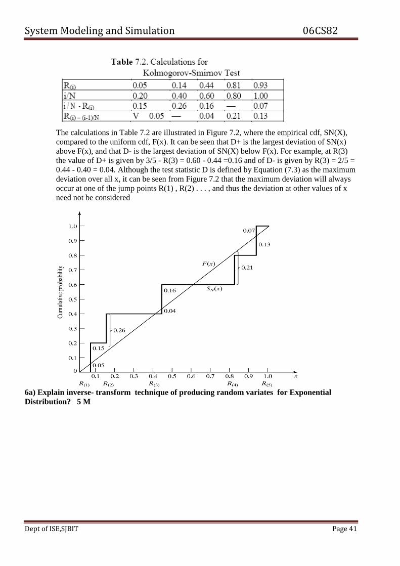
The calculations in Table 7.2 are illustrated in Figure 7.2, where the empirical cdf, SN(X), is
compared to the uniform cdf, F(x). It can be seen that D+ is the largest deviation of SN(x) above F(x),
System Modeling and Simulation 06CS82
Dept of ISE,SJBIT Page 24
and that D- is the largest deviation of SN(X) below F(x). For example, at R(3) the value of D
+ is given
by 3/5 - R(3) = 0.60 - 0.44 =0.16 and of D- is given by R(3) = 2/5 = 0.44 - 0.40 = 0.04. Although the
test statistic D is defined by Equation (7.3) as the maximum deviation over all x, it can be seen from
Figure 7.2 that the maximum deviation will always occur at one of the jump points R(1) , R(2) . . . ,
and thus the deviation at other values of x need not be considered.
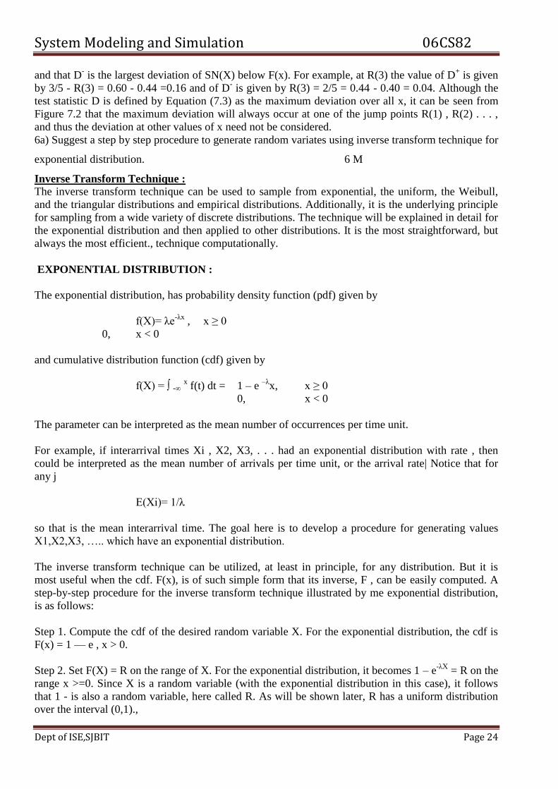
6a) Suggest a step by step procedure to generate random variates using inverse transform technique for
exponential distribution. 6 M
Inverse Transform Technique :
The inverse transform technique can be used to sample from exponential, the uniform, the Weibull,
and the triangular distributions and empirical distributions. Additionally, it is the underlying principle
for sampling from a wide variety of discrete distributions. The technique will be explained in detail for
the exponential distribution and then applied to other distributions. It is the most straightforward, but
always the most efficient., technique computationally.
EXPONENTIAL DISTRIBUTION :
The exponential distribution, has probability density function (pdf) given by
f(X)= λe-λx
, x ≥ 0
0, x < 0
and cumulative distribution function (cdf) given by
f(X) = ∫ -∞ x f(t) dt = 1 – e
–λx, x ≥ 0
0, x < 0
The parameter can be interpreted as the mean number of occurrences per time unit.
For example, if interarrival times Xi , X2, X3, . . . had an exponential distribution with rate , then
could be interpreted as the mean number of arrivals per time unit, or the arrival rate| Notice that for
any j
E(Xi)= 1/λ
so that is the mean interarrival time. The goal here is to develop a procedure for generating values
X1,X2,X3, ….. which have an exponential distribution.
The inverse transform technique can be utilized, at least in principle, for any distribution. But it is
most useful when the cdf. F(x), is of such simple form that its inverse, F , can be easily computed. A
step-by-step procedure for the inverse transform technique illustrated by me exponential distribution,
is as follows:
Step 1. Compute the cdf of the desired random variable X. For the exponential distribution, the cdf is
F(x) = 1 — e , x > 0.
Step 2. Set F(X) = R on the range of X. For the exponential distribution, it becomes 1 – e-λX
= R on the
range x >=0. Since X is a random variable (with the exponential distribution in this case), it follows
that 1 - is also a random variable, here called R. As will be shown later, R has a uniform distribution
over the interval (0,1).,

System Modeling and Simulation 06CS82
Dept of ISE,SJBIT Page 25
Step 3. Solve the equation F(X) = R for X in terms of R. For the exponential distribution, the solution
proceeds as follows:
1 – e-λ
x = R
e-λ
x= 1 – R
-λX= ln(1 - R)
x= -1/λ ln(1 – R) ( 5.1 )
Equation (5.1) is called a random-variate generator for the exponential distribution. In general,
Equation (5.1) is written as X=F-1(R ). Generating a sequence of values is accomplished through steps
4.
Step 4. Generate (as needed) uniform random numbers R1, R2, R3,... and compute the desired random
variates by
Xi = F-1 (Ri)
For the exponential case, F (R) = (-1/λ)ln(1- R) by Equation (5.1), so that
Xi = -1/λ ln ( 1 – Ri) ( 5.2 )
for i = 1,2,3,.... One simplification that is usually employed in Equation (5.2) is to
replace 1 – Ri by Ri to yield
Xi = -1/λ ln Ri ( 5.3 )
which is justified since both Ri and 1- Ri are uniformly distributed on (0,1).
6b) Enlist the steps involved in development of a useful model of input data. 6 M
There are four steps in the development of a useful model of input data:
• Collect data from the real system of interest. This often requires a substantial time and
resource commitment. Unfortunately, in some situations it is not possible to collect
data.
• Identify a probability distribution to represent the input process. When data are
available, this step typically begins by developing a frequency distribution, or
histogram, of the data.
• Choose parameters that determine a specific instance of the distribution family. When
data are available, these parameters may be estimated from the data.
• Evaluate the chosen distribution and the associated parameters for good-of-fit.
Goodness-of-fit may be evaluated informally via graphical methods, or formally via
statistical tests. The chisquare and the Kolmo-gorov-Smirnov tests are standard
goodness-of-fit tests. If not satisfied that the chosen distribution is a good
approximation of the data, then the analyst returns to the second step, chooses a
different family of distributions, and repeats the procedure. If several iterations of this
procedure fail to yield a fit between an assumed distributional form and the collected
data.
7a) Briefly explain the measures of performance of a simulation system. 10 M
Measures of performance
System Modeling and Simulation 06CS82
Dept of ISE,SJBIT Page 26
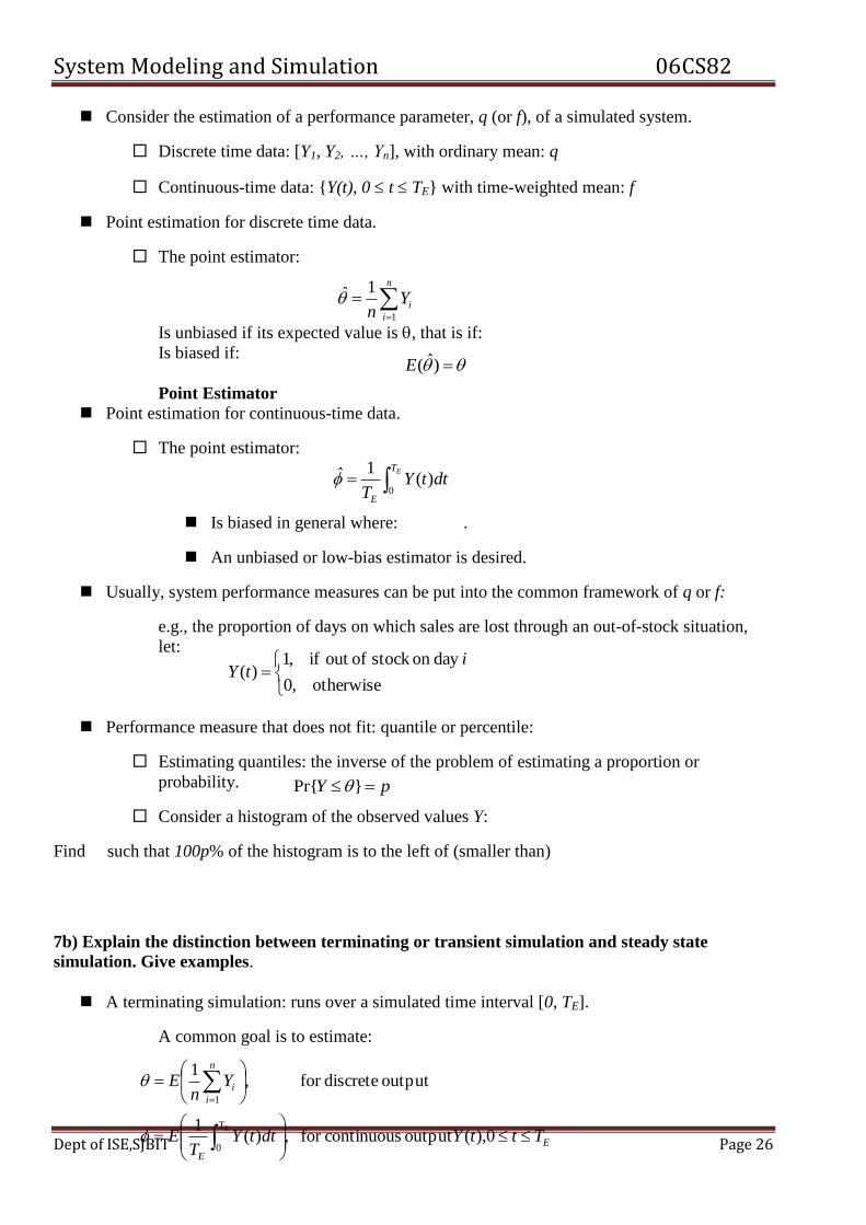
Consider the estimation of a performance parameter, q (or f), of a simulated system.
Discrete time data: [Y1, Y2, …, Yn], with ordinary mean: q
Continuous-time data: {Y(t), 0 t TE} with time-weighted mean: f
Point estimation for discrete time data.
The point estimator:
Is unbiased if its expected value is , that is if:
Is biased if:
Point Estimator
Point estimation for continuous-time data.
The point estimator:
Is biased in general where: .
An unbiased or low-bias estimator is desired.
Usually, system performance measures can be put into the common framework of q or f:
e.g., the proportion of days on which sales are lost through an out-of-stock situation,
let:
Performance measure that does not fit: quantile or percentile:
Estimating quantiles: the inverse of the problem of estimating a proportion or
probability.
Consider a histogram of the observed values Y:
Find such that 100p% of the histogram is to the left of (smaller than)
7b) Explain the distinction between terminating or transient simulation and steady state
simulation. Give examples.
A terminating simulation: runs over a simulated time interval [0, TE].
A common goal is to estimate:
n
i
iYn 1
1
)ˆ(E
ET
E
dttYT 0
)(1
otherwise ,0
day on stock ofout if ,1)(
itY
pY }Pr{
E
E
n
i
i
TttYdttYT
E
Yn
E
0),(output continuousfor ,)(1
output discretefor ,1
ET
0
1

System Modeling and Simulation 06CS82
Dept of ISE,SJBIT Page 27
In general, independent replications are used, each run using a different random number stream and
independently chosen initial conditions
8a) Explain with a neat diagram model building,verification and validation process 10 M
Verification of Simulation Models
• The purpose of model verification is to assure that the conceptual model is reflected accurately
in the computerized representation.
• The conceptual model quite often involves some degree of abstraction about system
operations, or some amount of simplification of actual operations.
Many suggestions can be given for use in the verification process:-
1: Have the computerized representation checked by someone other than its developer.
2: Make a flow diagram which includes each logically possible action a system can take when
an event occurs, and follow the model logic for each a for each action for each event type.
3: Closely examine the model output for reasonableness under a variety of settings of Input
parameters.
4. Have the computerized representation print the input parameters at the end of the Simulation
to be sure that these parameter values have not been changed inadvertently.
5. Make the computerized representation of self-documenting as possible.
6. If the computerized representation is animated, verify that what is seen in the animation
imitates the actual system.
7. The interactive run controller (IRC) or debugger is an essential component of Successful
simulation model building. Even the best of simulation analysts makes mistakes or commits
logical errors when building a model. The IRC assists in finding and correcting those errors in
the follow ways:
(a) The simulation can be monitored as it progresses.
(b) Attention can be focused on a particular line of logic or multiple lines of logic that
constitute a procedure or a particular entity.

System Modeling and Simulation 06CS82
Dept of ISE,SJBIT Page 28
(c) Values of selected model components can be observed. When the simulation has paused,
the current value or status of variables, attributes, queues, resources, counters, etc., can be
observed.
(d) The simulation can be temporarily suspended, or paused, not only to view information but
also to reassign values or redirect entities.
8. Graphical interfaces are recommended for accomplishing verification & validation .
8b) Describe the three steps approach to validation by Naylor and Finger. 10 M
Calibration and Validation of Models
• Verification and validation although are conceptually distinct, usually are conducted
simultaneously by the modeler.
• Validation is the overall process of comparing the model and its behavior to the real system
and its behavior.
• Calibration is the iterative process of comparing the model to the real system, making
adjustments to the model, comparing again and so on.
• The following figure 7.2 shows the relationship of the model calibration to the overall
validation process.
• The comparison of the model to reality is carried out by variety of test.
• Tests are subjective and objective.
• Subjective test usually involve people, who are knowledgeable about one or more aspects of
the system, making judgments about the model and its output.
• Objective tests always require data on the system's behavior plus the corresponding data
produced by the model.
As an aid in the validation process, Naylor and Finger [1967] formulated a three step approach
which has been widely followed:-
1. Build a model that has high face validity.

System Modeling and Simulation 06CS82
Dept of ISE,SJBIT Page 29
2. Validate model assumptions.
3. Compare the model input-output transformations to corresponding input-output
transformations for the real system.
Dec -2011
1a)List any five circumstances, When the Simulation is appropriate tool and when it is not?
10 M
Ans: When Simulation is the Appropriate Tool
Simulation enables the study of and experimentation with the internal interactions of a
complex system, or of a subsystem within a complex system.
Informational, organizational and environmental changes can be simulated and the effect
of those alternations on the model’s behavior can be observer.
The knowledge gained in designing a simulation model can be of great value toward
suggesting improvement in the system under investigation.
By changing simulation inputs and observing the resulting outputs, valuable insight may be
obtained into which variables are most important and how variables interact.
Simulation can be used as a pedagogical device to reinforce analytic solution
methodologies. Simulation can be used to experiment with new designs or policies prior to
implementation, so as to prepare for what may happen.
Simulation can be used to verify analytic solutions.
By simulating different capabilities for a machine, requirements can be determined.
When Simulation is Not Appropriate
Simulation should be used when the problem cannot be solved using common sense.
Simulation should not be used if the problem can be solved analytically.
Simulation should not be used, if it is easier to perform direct experiments.
Simulation should not be used, if the costs exceeds savings.
Simulation should not be performed, if the resources or time are not
available.
1b) Explain the steps in simulation study. With flow chart?10M
Steps in a Simulation study
1. Problem formulation
Every study begins with a statement of the problem, provided by policy makers.
Analyst ensures its clearly understood. If it is developed by analyst policy makers
should understand and agree with it.
2. Setting of objectives and overall project plan
The objectives indicate the questions to be answered by simulation. At this point a
determination should be made concerning whether simulation is the appropriate
methodology. Assuming it is appropriate, the overall project plan should include
A statement of the alternative systems
A method for evaluating the effectiveness of these alternatives
Plans for the study in terms of the number of people involved Cost of the study
The number of days required to accomplish each phase of the work with the
anticipated results.
3. Model conceptualization
The construction of a model of a system is probably as much art as science. The art of
modeling is enhanced by an ability
To abstract the essential features of a problem

System Modeling and Simulation 06CS82
Dept of ISE,SJBIT Page 30
To select and modify basic assumptions that characterize the system
To enrich and elaborate the model until a useful approximation results
Thus, it is best to start with a simple model and build toward greater complexity. Model
conceptualization enhance the quality of the resulting model and increase the
confidence of the model user in the application of the model.
4. Data collection
There is a constant interplay between the construction of model and the collection of
needed input data. Done in the early stages. Objective kind of data are to be collected.
5. Model translation
Real-world systems result in models that require a great deal of information storage and
computation. It can be programmed by using simulation languages or special purpose
simulation software.
Simulation languages are powerful and flexible. Simulation software models
development time can be reduced.
6. Verified
It pertains to he computer program and checking the performance. If the input
parameters and logical structure and correctly represented, verification is completed.
7. Validated
It is the determination that a model is an accurate representation of the real system.
Achieved through calibration of the model, an iterative process of comparing the model
to actual system behavior and the discrepancies between the two.
8. Experimental Design
The alternatives that are to be simulated must be determined. Which alternatives to
simulate may be a function of runs. For each system design, decisions need to be made
concerning
Length of the initialization period
Length of simulation runs
Number of replication to be made of each run
9. Production runs and analysis
They are used to estimate measures of performance for the system designs that are
being simulated.
10. More runs
Based on the analysis of runs that have been completed. The analyst determines if
additional runs are needed and what design those additional experiments should follow.
11. Documentation and reporting
Two types of documentation.
Program documentation
Process documentation
Program documentation
Can be used again by the same or different analysts to understand how the program
operates. Further modification will be easier. Model users can change the input
parameters for better performance.
Process documentation
Gives the history of a simulation project. The result of all analysis should be reported
clearly and concisely in a final report. This enable to review the final formulation and
alternatives, results of the experiments and the recommended solution to the problem.
The final report provides a vehicle of certification.
12. Implementation

System Modeling and Simulation 06CS82
Dept of ISE,SJBIT Page 31
Success depends on the previous steps. If the model user has been thoroughly involved
and understands the nature of the model and its outputs, likelihood of a vigorous
implementation is enhanced.
2a) Six dump trucks are used to have coal from the entrance of a mine to a railroad. Each truck
is loaded by one by one of the four loaders. After loading, a truck immediately moves to the
scale, to be weighed as soon as possible. Both the loader and the scale have first- come first-
served Waiting line for trucks. Travel time from a loader to scale is considered negligible. After
Being Weighed, a truck begins travel time [during which time truck unloads] and then
afterwards returns to loader queue. The activities of loading, Weighing and travel time are
given in the following table:
End of simulation is completion of Four Weighings from the scale. Depict the simulation table
estimate the loader and scale utilizations. Assume that Five of the trucks are at the loaders and
one is at the scale at Time θ.

System Modeling and Simulation 06CS82
Dept of ISE,SJBIT Page 32

System Modeling and Simulation 06CS82
Dept of ISE,SJBIT Page 33
2B) Explain simulation in GPSS With a block diagram, for the single server queue
simulation?
2c) Explain the following.
System :Acollectionofentitiesthatinteracttogetherovertimetoaccomplishoneormore goals.
Event List: Alistofeventnoticesforfutureevents,orderedbytimeofoccurrence;knownasthe
futureeventlist(FEL).
Alwaysrankedbytheeventtime
Entity:Anobjectinthesystemthatrequiresexplicitrepresentationinthemodel,e.g.,people,
machines,nodes,packets,server,customer
Event: Aninstantaneousoccurrencethatchangesthestateofasystem.
3a) Explain discrete random variable and continuous random variable with an example?
10M
Discrete Random Variables [Probability Review]
X is a discrete random variable if the number of possible
values of X is finite, or countably infinite.
Example: Consider jobs arriving at a job shop. Let X be the number of jobs arriving each week at a job shop.
Rx = possible values of X (range space of X) = {0,1,2,…}
p(xi) = probability the random variable is xi = P(X = xi)
p(xi), i = 1,2, … must satisfy:
The collection of pairs [xi, p(xi)], i = 1,2,…, is called the probability
distribution of X, and p(xi) is called the probability mass function
(pmf) of X.
11)( 2.
allfor ,0)( 1.
i i
i
xp
ixp
System Modeling and Simulation 06CS82
Dept of ISE,SJBIT Page 34
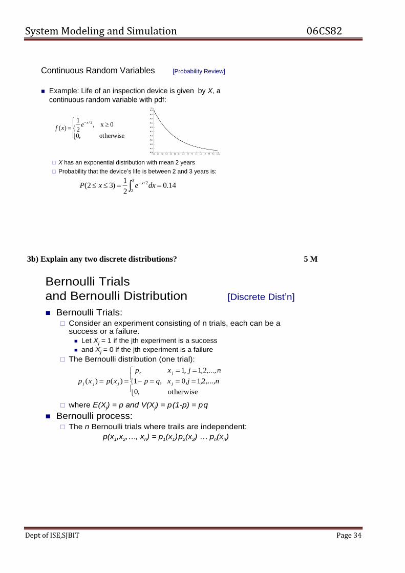
3b) Explain any two discrete distributions? 5 M
Continuous Random Variables [Probability Review]
Example: Life of an inspection device is given by X, a
continuous random variable with pdf:
X has an exponential distribution with mean 2 years
Probability that the device’s life is between 2 and 3 years is:
otherwise ,0
0 x,2
1
)(2/xe
xf
14.02
1)32(
3
2
2/ dxexP x
Bernoulli Trials
and Bernoulli Distribution [Discrete Dist’n]
Bernoulli Trials: Consider an experiment consisting of n trials, each can be a
success or a failure.
Let Xj = 1 if the jth experiment is a success
and Xj = 0 if the jth experiment is a failure
The Bernoulli distribution (one trial):
where E(Xj) = p and V(Xj) = p(1-p) = pq
Bernoulli process: The n Bernoulli trials where trails are independent:
p(x1,x2,…, xn) = p1(x1)p2(x2) … pn(xn)
otherwise ,0
210 ,1
,...,2,1,1 ,
)()( ,...,n,,jxqp
njxp
xpxp j
j
jjj

System Modeling and Simulation 06CS82
Dept of ISE,SJBIT Page 35
3c) explain the following continuous distributions?
i) Uniform Distribution
ii) Exponentioal Distribution
Binomial Distribution [Discrete Dist’n]
The number of successes in n Bernoulli trials, X, has a
binomial distribution.
The mean, E(x) = p + p + … + p = n*p
The variance, V(X) = pq + pq + … + pq = n*pq
The number of
outcomes having the
required number of
successes and
failures
Probability that
there are
x successes and
(n-x) failures
otherwise ,0
,...,2,1,0 , )(
nxqpx
n
xpxnx
Uniform Distribution [Continuous Dist’n]
A random variable X is uniformly distributed on the
interval (a,b), U(a,b), if its pdf and cdf are:
Properties
P(x1 < X < x2) is proportional to the length of the interval [F(x2) –
F(x1) = (x2-x1)/(b-a)]
E(X) = (a+b)/2 V(X) = (b-a)2/12
U(0,1) provides the means to generate random numbers,
from which random variates can be generated.
otherwise ,0
,1
)(bxa
abxf
bx
bxaab
axax
xF
,1
,
,0
)(

System Modeling and Simulation 06CS82
Dept of ISE,SJBIT Page 36
4a) Explain the characterisitcs of queuing system? And Explain the notations of queuing
system? 10 M
Calling Population [Characteristics of Queueing System]
Calling population: the population of potential customers, may be assumed to be finite or
infinite.
Finite population model: if arrival rate depends on the number of customers being
served and waiting, e.g., model of one corporate jet, if it is being repaired, the repair
arrival rate becomes zero.
Infinite population model: if arrival rate is not affected by the number of customers
being served and waiting, e.g., systems with large population of potential customers.
System Capacity [Characteristics of Queueing System]
System Capacity: a limit on the number of customers that may be in the waiting line or system.
Limited capacity, e.g., an automatic car wash only has room for 10 cars to wait in line
to enter the mechanism.
Unlimited capacity, e.g., concert ticket sales with no limit on the number of people
allowed to wait to purchase tickets.
Arrival Process [Characteristics of Queueing System]
For infinite-population models:
In terms of interarrival times of successive customers.
Random arrivals: interarrival times usually characterized by a probability distribution.
Exponential Distribution [Continuous Dist’n]
A random variable X is exponentially distributed with
parameter > 0 if its pdf and cdf are:
elsewhere ,0
0 ,)(
xexf
x
0 ,1
0 0,)(
0xedte
xxF x
xt
E(X) = 1/ V(X) = 1/2
Used to model interarrival times
when arrivals are completely
random, and to model service
times that are highly variable
For several different exponential
pdf’s (see figure), the value of
intercept on the vertical axis is ,
and all pdf’s eventually intersect.

System Modeling and Simulation 06CS82
Dept of ISE,SJBIT Page 37
Most important model: Poisson arrival process (with rate l), where An
represents the interarrival time between customer n-1 and customer n, and is
exponentially distributed (with mean 1/l).
Scheduled arrivals: interarrival times can be constant or constant plus or minus a small
random amount to represent early or late arrivals.
e.g., patients to a physician or scheduled airline flight arrivals to an airport.
At least one customer is assumed to always be present, so the server is never idle, e.g.,
sufficient raw material for a machine.
Arrival Process [Characteristics of Queueing System]
For finite-population models:
Customer is pending when the customer is outside the queueing system, e.g., machine-
repair problem: a machine is ―pending‖ when it is operating, it becomes ―not pending‖
the instant it demands service form the repairman.
Runtime of a customer is the length of time from departure from the queueing system
until that customer’s next arrival to the queue, e.g., machine-repair problem, machines
are customers and a runtime is time to failure.
Let A1(i), A2(i), … be the successive runtimes of customer i, and S1(i), S2(i) be the
corresponding successive system times:
Queue Behavior and Queue Discipline [Characteristics of Queueing System]
Queue behavior: the actions of customers while in a queue waiting for service to begin, for
example:
Balk: leave when they see that the line is too long,
Renege: leave after being in the line when its moving too slowly,
Jockey: move from one line to a shorter line.
Queue discipline: the logical ordering of customers in a queue that determines which customer
is chosen for service when a server becomes free, for example:
First-in-first-out (FIFO)
Last-in-first-out (LIFO)

System Modeling and Simulation 06CS82
Dept of ISE,SJBIT Page 38
Service in random order (SIRO)
Shortest processing time first (SPT)
Service according to priority (PR).
Queueing Notation
[Characteristics of Queueing System]
A notation system for parallel server queues: A/B/c/N/K
A represents the interarrival-time distribution,
B represents the service-time distribution,
c represents the number of parallel servers,
N represents the system capacity,
K represents the size of the calling population.
Primary performance measures of queueing systems:
Pn: steady-state probability of having n customers in system,
Pn(t): probability of n customers in system at time t,
l: arrival rate,
le: effective arrival rate,
m: service rate of one server,
r: server utilization,
An: interarrival time between customers n-1 and n,
Sn: service time of the nth arriving customer,
Wn: total time spent in system by the nth arriving customer,
WnQ: total time spent in the waiting line by customer n,
L(t): the number of customers in system at time t,
LQ(t): the number of customers in queue at time t,
L: long-run time-average number of customers in system,
LQ: long-run time-average number of customers in queue,
w : long-run average time spent in system per customer,
wQ: long-run average time spent in queue per customer.
4b) Explain any two long run measure of performance queuing system? 10 M

System Modeling and Simulation 06CS82
Dept of ISE,SJBIT Page 39
5a) Explain the two different techniques for generating random numbers with examples?
1 Linear Congruential Method
Time-Average Number in System L[Characteristics of Queueing System]
Consider a queueing system over a period of time T,
Let Ti denote the total time during [0,T] in which the system
contained exactly i customers, the time-weighted-average number
in a system is defined by:
Consider the total area under the function is L(t), then,
The long-run time-average # in system, with probability 1:
00
1ˆ
i
i
i
iT
TiiT
TL
T
i
i dttLT
iTT
L0
0
)(11ˆ
TLdttLT
LT
as )(1ˆ
0
Server Utilization[Characteristics of Queueing System]
For G/G/1/∞/∞ queues:
Any single-server queueing system with average arrival
rate customers per time unit, where average service time
E(S) = 1/ time units, infinite queue capacity and calling
population.
Conservation equation, L = w, can be applied.
For a stable system, the average arrival rate to the server,
s, must be identical to .
The average number of customers in the server is:
T
TTdttLtL
TL
T
Qs0
0)()(
1ˆ
Server Utilization and System Performance[Characteristics of Queueing System]
Example: A physician who schedules patients every 10 minutes and
spends Si minutes with the ith patient:
Arrivals are deterministic, A1 = A2 = … = -1 = 10.
Services are stochastic, E(Si) = 9.3 min and V(S0) = 0.81 min2.
On average, the physician's utilization = = 0.93 < 1.
Consider the system is simulated with service times: S1 = 9, S2 =
12, S3 = 9, S4 = 9, S5 = 9, …. The system becomes:
The occurrence of a relatively long service time (S2 = 12) causes a
waiting line to form temporarily.
1.0y probabilit with minutes 12
9.0y probabilit with minutes 9iS

System Modeling and Simulation 06CS82
Dept of ISE,SJBIT Page 40
The linear congruential method, initially proposed by Lehmer [1951], produces a
sequence of
integers, X\, X2,... between zero and m — 1 according to the following recursive relationship:
The initial value X0 is called the seed,
If c ≠ 0 in Equation (7.1), the form is called the mixed congruential method.When c = 0, the form is
known as the multiplicative congruential method. The selection of the values for a, c, m and X0
drastically affects the statistical properties and the cycle length. . The random integers are being
generated [0,m-1], and to convert the integers to random numbers:
2 Combined Linear Congruential Generators
As computing power has increased, the complexity of the systems that we are able to simulate has also
increased.
One fruitful approach is to combine two or more multiplicative congruen-tial generators in such a way
that the combined generator has good statistical properties and a longer period. The following result
from L'Ecuyer [1988] suggests how this can be done: If Wi, 1 , Wi , 2. . . , W i,kare any independent,
discrete-valued random variables (not necessarily identically distributed), but one of them, say Wi, 1,
is uniformly distributed on the integers 0 to mi — 2, then is uniformly distributed on the integers 0 to
mi — 2.
5b) The sequence of numbers 0.44,0.81,0.14,0.05,0.93 were generated, use the Kolmogorov-
Smirnov test with a level of significance a of 0.05.compare F(X) and SN(X) 10 M
,...2,1,0 , mod )(1 imcaXX ii
The multiplier
The increment
The modulus
System Modeling and Simulation 06CS82
Dept of ISE,SJBIT Page 41
The calculations in Table 7.2 are illustrated in Figure 7.2, where the empirical cdf, SN(X),
compared to the uniform cdf, F(x). It can be seen that D+ is the largest deviation of SN(x)
above F(x), and that D- is the largest deviation of SN(X) below F(x). For example, at R(3)
the value of D+ is given by 3/5 - R(3) = 0.60 - 0.44 =0.16 and of D- is given by R(3) = 2/5 =
0.44 - 0.40 = 0.04. Although the test statistic D is defined by Equation (7.3) as the maximum
deviation over all x, it can be seen from Figure 7.2 that the maximum deviation will always
occur at one of the jump points R(1) , R(2) . . . , and thus the deviation at other values of x
need not be considered
6a) Explain inverse- transform technique of producing random variates for Exponential
Distribution? 5 M

System Modeling and Simulation 06CS82
Dept of ISE,SJBIT Page 42
6b) Genarate Three poison variates with mean α=0.2 5M
Exponential Distribution [Inverse-transform]
Exponential Distribution:
Exponential cdf:
To generate X1, X2, X3 …
r = F(x)
= 1 – e-x for x 0
R=F(X)
X=F-1(R)
Xi = F-1(Ri)
= -(1/ ln(1-Ri)
= - (1/) ln(Ri)
Since both 1-Ri & Ri are uniformly distributed between 0& 1
Figure: Inverse-transform
technique for exp( = 1)

System Modeling and Simulation 06CS82
Dept of ISE,SJBIT Page 43
6c) Explain the types of simulationwith respect to the output Analysis? Give at least two
examples? 10 M
Type of Simulations
Terminating verses non-terminating simulations
Terminating simulation:
Runs for some duration of time TE, where E is a specified event
that stops the simulation.
Starts at time 0 under well-specified initial conditions.
Ends at the stopping time TE.
Bank example: Opens at 8:30 am (time 0) with no customers
present and 8 of the 11 teller working (initial conditions), and
closes at 4:30 pm (Time TE = 480 minutes).
The simulation analyst chooses to consider it a terminating
system because the object of interest is one day’s operation.

System Modeling and Simulation 06CS82
Dept of ISE,SJBIT Page 44
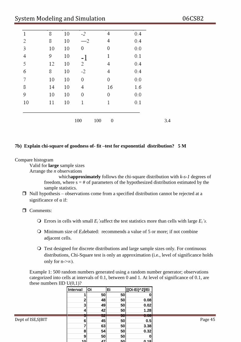
7a) Explain the chi-square test with a = 0.05 to test whether the data shown below are
uniformly distributed. Table 7.3 contains the essential computations. The test uses n = 10
intervals of equal length, namely (0, 0.1], (0.1, 0.2], . . . , (0.9, 1.0]. The value of χ0 2
is 3.4. This is
compared with the critical value χ2
0.05, 9 =16.9.Since χ0 2
is much smaller than the tabulated value
of χ20.05, 9 the null hypothesis of a uniform distribution is not rejected.
Type of Simulations
Non-terminating simulation:
Runs continuously, or at least over a very long period of time.
Examples: assembly lines that shut down infrequently, telephone
systems, hospital emergency rooms.
Initial conditions defined by the analyst.
Runs for some analyst-specified period of time TE.
Study the steady-state (long-run) properties of the system,
properties that are not influenced by the initial conditions of the
model.
Whether a simulation is considered to be terminating or
non-terminating depends on both
The objectives of the simulation study and
The nature of the system.
Interval OiEiOi-Ei (Oi-Ei)2 (Oi-Ei)
2 /Ei
System Modeling and Simulation 06CS82
Dept of ISE,SJBIT Page 45
100 100 0 3.4
7b) Explain chi-square of goodness of- fit –test for exponential distribution? 5 M
Compare histogram
Valid for large sample sizes
Arrange the n observations
whichapproximately follows the chi-square distribution with k-s-1 degrees of
freedom, where s = # of parameters of the hypothesized distribution estimated by the
sample statistics.
Null hypothesis – observations come from a specified distribution cannot be rejected at a
significance of α if:
Comments:
Errors in cells with small Ei’saffect the test statistics more than cells with large Ei’s.
Minimum size of Eidebated: recommends a value of 5 or more; if not combine
adjacent cells.
Test designed for discrete distributions and large sample sizes only. For continuous
distributions, Chi-Square test is only an approximation (i.e., level of significance holds
only for n->∞).
Example 1: 500 random numbers generated using a random number generator; observations
categorized into cells at intervals of 0.1, between 0 and 1. At level of significance of 0.1, are
these numbers IID U(0,1)?
Interval Oi Ei [(Oi-Ei)^2]/Ei
1 50 50 0
2 48 50 0.08
3 49 50 0.02
4 42 50 1.28
5 52 50 0.08
6 45 50 0.5
7 63 50 3.38
8 54 50 0.32
9 50 50 0
10 47 50 0.18
500 5.84

System Modeling and Simulation 06CS82
Dept of ISE,SJBIT Page 46
8a) Explain a model building, and verification and validation? 10M
Modeling-Building, Verification & Validation
0.10. of level cesignificanat accepted Hypothesis
;68.14 table thefrom ;85.5 2
]9,9.0[
2
0
System Modeling and Simulation 06CS82
Dept of ISE,SJBIT Page 47
8b) Explain any two output analysis for steady-state simulation? 10M
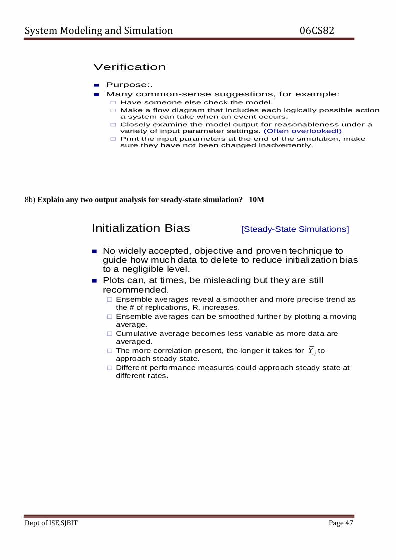
Verification
Purpose:.
Many common-sense suggestions, for example:
Have someone else check the model.
Make a flow diagram that includes each logically possible action
a system can take when an event occurs.
Closely examine the model output for reasonableness under a
variety of input parameter settings. (Often overlooked!)
Print the input parameters at the end of the simulation, make
sure they have not been changed inadvertently.
Initialization Bias [Steady-State Simulations]
No widely accepted, objective and proven technique to guide how much data to delete to reduce initialization bias to a negligible level.
Plots can, at times, be misleading but they are still recommended. Ensemble averages reveal a smoother and more precise trend as
the # of replications, R, increases.
Ensemble averages can be smoothed further by plotting a moving average.
Cumulative average becomes less variable as more data are averaged.
The more correlation present, the longer it takes for to approach steady state.
Different performance measures could approach steady state at different rates.
jY.

System Modeling and Simulation 06CS82
Dept of ISE,SJBIT Page 48
Error Estimation [Steady-State Simulations]
For a covariance stationary time series, {Y1, …, Yn}:
Lag-k autocovariance is:
Lag-k autocorrelation is:
If a time series is covariance stationary, then the variance
of is:
The expected value of the variance estimator is:
Y
),cov(),cov( 11 kiikk YYYY
2
k
k
1
1
2
121)(n
k
kn
k
nYV
1
1/ e wher,)(
2
n
cnBYBV
n
SE
c
Error Estimation [Steady-State Simulations]
a) Stationary time series Yi
exhibiting positive
autocorrelation.
b) Stationary time series Yi
exhibiting negative
autocorrelation.
c) Nonstationary time series with
an upward trend

System Modeling and Simulation 06CS82
Dept of ISE,SJBIT Page 49
June -2011
1) a) What is system And System Environment? Explain the components of a system with an
example? 10 M
Ans:System
A system is defined as an aggregation or assemblage of objects joined in some
regular interaction or interdependence toward the accomplishment of some purpose.
Example : Production System
Production Control System
Purchasing Fabrication Assembly Shipping
Department Department Department Department
System Environment
The external components which interact with the system and produce necessary
changes are said to constitute the system environment. In modeling systems, it is
necessary to decide on the boundary between the system and its environment. This
decision may depend on the purpose of the study.
Components of a System
Entity -An entity is an object of interest in a system.
Ex: In the factory system, departments, orders, parts and products are The entities.
Attribute-An attribute denotes the property of an entity.
Ex: Quantities for each order, type of part, or number of machines in a Department are
attributes of factory system.
Activity-Any process causing changes in a system is called as an activity.
Ex: Manufacturing process of the department.
State of the System-The state of a system is defined as the collection of variables
necessary to describe a system at any time, relative to the objective of study. In other
words, state of the system mean a description of all the entities, attributes and activities
as they exist at one point in time.
Event-An event is define as an instantaneous occurrence that may change the state of
the system.
1b) Explain various steps in simulation study. With help of neat diagram? 10 M 1. Problem formulation

System Modeling and Simulation 06CS82
Dept of ISE,SJBIT Page 50
Every study begins with a statement of the problem, provided by policy makers.
Analyst ensures its clearly understood. If it is developed by analyst policy makers
should understand and agree with it.
2. Setting of objectives and overall project plan
The objectives indicate the questions to be answered by simulation. At this point a
determination should be made concerning whether simulation is the appropriate
methodology. Assuming it is appropriate, the overall project plan should include
A statement of the alternative systems
A method for evaluating the effectiveness of these alternatives
Plans for the study in terms of the number of people involved Cost of the study
The number of days required to accomplish each phase of the work with the
anticipated results.
3. Model conceptualization
The construction of a model of a system is probably as much art as science. The art of
modeling is enhanced by an ability
.To abstract the essential features of a problem
To select and modify basic assumptions that characterize the system
To enrich and elaborate the model until a useful approximation results
Thus, it is best to start with a simple model and build toward greater complexity. Model
conceptualization enhance the quality of the resulting model and increase the
confidence of the model user in the application of the model.
4. Data collection There is a constant interplay between the construction of model and the collection of
needed input data. Done in the early stages. Objective kind of data are to be collected.
5. Model translation
Real-world systems result in models that require a great deal of information storage and
computation. It can be programmed by using simulation languages or special purpose
simulation software.
6. Verified
It pertains to he computer program and checking the performance. If the input
parameters and logical structure and correctly represented, verification is completed.
7. Validated
It is the determination that a model is an accurate representation of the real system.
Achieved through calibration of the model, an iterative process of comparing the model
to actual system behavior and the discrepancies between the two.
8. Experimental Design
The alternatives that are to be simulated must be determined. Which alternatives to
simulate may be a function of runs. For each system design, decisions need to be made
concerning
Length of the initialization period
Length of simulation runs
Number of replication to be made of each run
9. Production runs and analysis
They are used to estimate measures of performance for the system designs that are
being simulated.
10. More runs

System Modeling and Simulation 06CS82
Dept of ISE,SJBIT Page 51
Based on the analysis of runs that have been completed. The analyst determines if
additional runs are needed and what design those additional experiments should follow.
11. Documentation and reporting
Two types of documentation.
Program documentation
Process documentation
Program documentation
Can be used again by the same or different analysts to understand how the program
operates. Further modification will be easier. Model users can change the input
parameters for better performance.
Process documentation
Gives the history of a simulation project. The result of all analysis should be reported
clearly and concisely in a final report. This enable to review the final formulation and
alternatives, results of the experiments and the recommended solution to the problem.
The final report provides a vehicle of certification.
12. Implementation
Success depends on the previous steps. If the model user has been thoroughly involved
and understands the nature of the model and its outputs, likelihood of a vigorous
implementation is enhanced.
Steps in simulation study
2a) With the help of flow diagram, Explain the single channel queuing system. 10M Ans: Simulation of Queuing systems

System Modeling and Simulation 06CS82
Dept of ISE,SJBIT Page 52
A queueing system is described by its calling population, the nature of the arrivals, the service
mechanism, the system capacity, and the queueing discipline. A single-channel queueing system is
portrayed in figure1.
In the single-channel queue, the calling population is infinite; that is, if a unit leaves
the alling
population and joins the waiting line or enters service, there is no change in the arrival
rate of other units that may need service.
Arrivals for service occur one at a time in a random fashion; once they join the
waiting line, they are eventually served. In addition, service times are of some random
length according to a probability distribution which does not change over time.
The system capacity; has no limit, meaning that any number of units can wait in
line. Finally, units are served in the order of their arrival by a single server or
channel.
Arrivals and services are defined by the distributions of the time between arrivals
and the distribution of service times, respectively.
For any simple single or multi-channel queue, the overall effective arrival rate must
be less than the total service rate, or the waiting line will grow without bound. When
queues grow without bound, they are termed “explosive” or unstable.
The state of the system is the number of units in the system and the status of the
server, busy or idle.
An event is a set of circumstances that cause an instantaneous change in the state of
the system. In a single –channel queueing system there are only two possible events
that can affect the state of the system.
They are the entry of a unit into the system
The completion of service on a unit.

System Modeling and Simulation 06CS82
Dept of ISE,SJBIT Page 53
The queueing system includes the server, the unit being serviced, and units in the queue.
thesimulation clock is used to track simulated time. If a unit has just completed service, the
simulation proceeds in the manner shown in the flow diagram of figure.2. Note that the server
has only two possible states: it is either busy or idle.
The arrival event occurs when a unit enters the system. The flow diagram for the arrival
event is shown in figure 3. The unit may find the server either idle or busy; therefore,
either the unit begins service immediately, or it enters the queue for the server. The unit
follows the course of action shown in fig 4.
If the server is busy, the unit enters the queue. If the server is idle and the queue is
empty, the unit begins service. It is not possible for the server to be idle and the queue
to be nonempty
2b) A large milling machine has three different bearings that fail in service.The cumulative
distribution function of the life of each bearing is identical given in table 1. When a bearing
fails,the mill stops,a repair person is called and a new bearing is installed.the delay time of the
repair person’s arriving at the milling machine is also a randon variuable,with the distribution
given in table 2.Downtime for the mill is esrimated at $5/minute.The direct on site cost of the
repair person is $15/hour.It takes 20 minutes to change 1 bearing,30 minutes to change 2
bearings and 40 minutes to change 3 bearings .The bearing cost is $16 each.Aproposal has been
made to replace all 3 bearings whenever a bearing fails.Management needs an evaluation of this

System Modeling and Simulation 06CS82
Dept of ISE,SJBIT Page 54
proposal. Simulate the system for 10,000 hours of operaion under proposed method and
determine the total cost of the proposed system.
Table 1 Bearing life distribution
Bearing
Life(Hrs)
1000 1100 1200 1300 1400 1500 1600 1700 1800 1900
Probability 0.10 0.13 0.25 0.13 0.09 0.12 0.02 0.06 0.05 0.05
Table 2 Delay time distribution
Delay(minutes) 5 10 15
Probability 0.6 0.3 0.1
Consider the following sequence of random digits for bearing life times
Bearing 1 67 8 49 84 44 30 10 15
Bearing 2 70 43 86 93 81 44 19 51
Bearing 3 76 65 61 96 65 56 11 86
Consider the following sequence of random digits for delay time
Delay 3 7 5 1 4 3 7 8

System Modeling and Simulation 06CS82
Dept of ISE,SJBIT Page 55
2.3 Other Examples of Simulation (2)
• Example 2.5 (Cont.)
The cumulative distribution function of the life of each bearing is identical, as shown in Table 2.22.
The delay time of the repairperson's arriving at the milling machine is also a random variable, with the distribution given in Table 2.23.

System Modeling and Simulation 06CS82
Dept of ISE,SJBIT Page 56
3a) what do you mean by World View? Discuss the different types of World View? 10M
Ans: World Views Process-interaction
• Modelerthinksintermsofprocesses
• Aprocessisthelifecycleofoneentity,whichconsistsofvariouseventsandactivities
•Simulationmodelisdefinedintermsofentitiesorobjectsandtheirlifecycleastheyflow throughthesystem,demandingresourcesandqueueingtowaitforresources
• Someactivitiesmightrequiretheuseofoneormoreresourceswhosecapacitiesarelimited
• Processesinteract,e.g.,oneprocesshastowaitinaqueuebecausetheresourceitneedsis busywithanotherprocess
• Aprocessisatime-sequencedlistofevents,activitiesanddelays,includingdemandsfor resource,thatdefinethelifecycleofoneentityasitmovesthroughasystem
• Variabletimeadvance
Activity-scanning
• Modelerconcentrates on activities of a model and those conditions that allowan
activityto begin
• At each clock advance, the conditions foreach activity are checked,and,if the
conditions are true,thenthecorresponding
activitybegins
• Fixtimeadvance
• Disadvantage: The repeated scanning to discover whether an
activitycanbeginresultsinslow runtime
Improvement: Three-phase approach
- Combinationofeventscheduling withactivityscannig
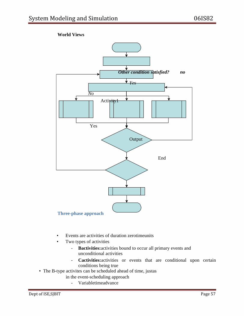
System Modeling and Simulation 06IS82
Dept of ISE,SJBIT Page 57
World Views
Other condition satisfied? no
Yes
No
Activity1
Yes
Output End Three-phase approach
• Events are activities of duration zerotimeunits
• Two types of activities
- Bactivities:activities bound to occur all primary events and unconditional activities
- Cactivities:activities or events that are conditional upon certain conditions being true
• The B-type activites can be scheduled ahead of time, justas
in the event-scheduling approach
- Variabletimeadvance

System Modeling and Simulation 06IS82
Dept of ISE,SJBIT Page 58
- FELcontainsonlyB-typeevents
• Scanning to learn whetherany C- type activities can begin orC-type events occur
happen only at the end of each time advance, after
all B-type events have completed
3b) The maximum inventory level, M, is 11 units and the review period, N, is 5 days. The
problem is to estimate, by simulation, the average ending units in inventory and the
number of days when a shortage condition occurs. The distribution of the number of units
demanded per day is shown in table 9. In this example, lead-time is a random variable, as
shown in table 10. Assume that orders are placed at the close of business and are received
for inventory at the beginning as determined by the lead-time.
ANS: Simulation of an (M, N) Inventory System

System Modeling and Simulation 06IS82
Dept of ISE,SJBIT Page 59
4 a) What is the role of maximum density and maximum period in generation of random
numbers? With given seed 27, constant multiplier 17, increment 43 and modulus 100. And
generate Five random numbers?
Ans : These random integers should appear to be uniformly distributed the integers zero to 99.
Random numbers between zero and 1 can be generated by
Ri =Xi/m, i= 1,2,…… (7.2)
The sequence of Xi and subsequent Ri values is computed as follows:
X0 = 27
X1 = (17.27 + 43) mod 100 = 502 mod 100 = 2 R1=2⁄100=0. 02
X2 = (17 • 2 + 43) mod 100 = 77 mod 100 = 77 R2=77 ⁄100=0. 77
X3 = (17•77+ 43) mod 100 = 1352 mod 100 = 52 R3=52 ⁄100=0. 52
4 b) Out of syllabus

System Modeling and Simulation 06IS82
Dept of ISE,SJBIT Page 60
5 a) what is inverse transform technique? Derive an expression for Exponentional
Distribution?
Develop understanding of generating samples from a specified distribution as input to a simulation model.
Illustrate some widely-used techniques for generating random variates. Inverse-transform technique
Acceptance-rejection technique
Special properties
Inverse-transform Technique The concept:
For cdf function: r = F(x)
Generate r from uniform (0,1)
Find x:
Random-Variate Generation
x = F-1(r)
r1
x1
r = F(x)
5 b) A Sequence of 1000 four digits has been generated and analysis indicates the
following combinations & frequencies, Based on poker test check whether the numbers
are independent. Use α=0.05, X2
0,05,2=5.99
Exponential Distribution [Inverse-transform]
Exponential Distribution:
Exponential cdf:
To generate X1, X2, X3 …
r = F(x)
= 1 – e-x for x 0
R=F(X)
X=F-1(R)
Xi = F-1(Ri)
= -(1/ ln(1-Ri)
= - (1/) ln(Ri)
Since both 1-Ri & Ri are uniformly distributed between 0& 1
Combinations (i) OI
Four different
digit
One fair
Two Pair
Three like digit
565
392
17
24
2

System Modeling and Simulation 06IS82
Dept of ISE,SJBIT Page 61
Ans:
Combi
nation i
Obse
rved
OI
Exp
ecte
d Ei
(Oi
-
Ei)
2/E
i
4
differen
t digit
565
504
7.3
8
1 pair 392 432 3.7
0
2 pair 17 27 3.7
0
3 like
digits
24 36
4 like
digits
2 1 3.2
7
Total 1000 1000 18.
060
6
X2
0,05, 3=7.81< X2
0=18.0806
6a) What is Acceptence-Rejection Technique? Generate three poison variates with mean
α=0.2 10 M
Ans: Procedure of generating a Poisson random variate N is as follows
1. Set n=0, P=1
2. Generate a random number Rn+1, and replace P by P. ( Rn+1)
3. If P <exp(-α), then accept N=n
- Otherwise, reject the current n, increase n
by one, and return to step 2.
Four like digit

System Modeling and Simulation 06IS82
Dept of ISE,SJBIT Page 62
6 b) out of syllabus
7a) What do you mean by verification and validation of simulation models? Explain
calibration and validation of models with neat diagram? 10M
Verification
Purpose:.
Many common-sense suggestions, for example:
Have someone else check the model.
Make a flow diagram that includes each logically possible action
a system can take when an event occurs.
Closely examine the model output for reasonableness under a
variety of input parameter settings. (Often overlooked!)
Print the input parameters at the end of the simulation, make
sure they have not been changed inadvertently.

System Modeling and Simulation 06IS82
Dept of ISE,SJBIT Page 63
Modeling-Building, Verification & Validation
Purpose & Overview
The goal of the validation process is:
To produce a model that represents true behavior closely
enough for decision-making purposes
To increase the model’s credibility to an acceptable level
Validation is an integral part of model development
Verification – building the model correctly (correctly implemented
with good input and structure)
Validation – building the correct model (an accurate
representation of the real system)
Most methods are informal subjective comparisons while
a few are formal statistical procedures

System Modeling and Simulation 06IS82
Dept of ISE,SJBIT Page 64
7b) Discuss types of simulations With respect of output Analysis with Example? 10M
Type of Simulations
Terminating verses non-terminating simulations
Terminating simulation:
Runs for some duration of time TE, where E is a specified event
that stops the simulation.
Starts at time 0 under well-specified initial conditions.
Ends at the stopping time TE.
Bank example: Opens at 8:30 am (time 0) with no customers
present and 8 of the 11 teller working (initial conditions), and
closes at 4:30 pm (Time TE = 480 minutes).
The simulation analyst chooses to consider it a terminating
system because the object of interest is one day’s operation.

System Modeling and Simulation 06IS82
Dept of ISE,SJBIT Page 65
8 Write a Short note on 20 M
a) Characteristics of queuing system?
Characteristics of Queueing Systems
Key elements of queueing systems:
Customer: refers to anything that arrives at a facility and requires service, e.g.,
people, machines, trucks, emails.
Server: refers to any resource that provides the requested service, e.g.,
repairpersons, retrieval machines, runways at airport.
Calling Population [Characteristics of Queueing System]
Calling population: the population of potential customers, may be assumed to be finite or
infinite.
Type of Simulations
Non-terminating simulation:
Runs continuously, or at least over a very long period of time.
Examples: assembly lines that shut down infrequently, telephone
systems, hospital emergency rooms.
Initial conditions defined by the analyst.
Runs for some analyst-specified period of time TE.
Study the steady-state (long-run) properties of the system,
properties that are not influenced by the initial conditions of the
model.
Whether a simulation is considered to be terminating or
non-terminating depends on both
The objectives of the simulation study and
The nature of the system.

System Modeling and Simulation 06IS82
Dept of ISE,SJBIT Page 66
Finite population model: if arrival rate depends on the number of customers being
served and waiting, e.g., model of one corporate jet, if it is being repaired, the
repair arrival rate becomes zero.
Infinite population model: if arrival rate is not affected by the number of
customers being served and waiting, e.g., systems with large population of
potential customers.
System Capacity [Characteristics of Queueing System]
System Capacity: a limit on the number of customers that may be in the waiting line or
system.
Limited capacity, e.g., an automatic car wash only has room for 10 cars to wait in
line to enter the mechanism.
Unlimited capacity, e.g., concert ticket sales with no limit on the number of
people allowed to wait to purchase tickets.
Arrival Process [Characteristics of Queueing System]
For infinite-population models:
In terms of interarrival times of successive customers.
Random arrivals: interarrival times usually characterized by a probability
distribution.
Most important model: Poisson arrival process (with rate l), where An
represents the interarrival time between customer n-1 and customer n, and
is exponentially distributed (with mean 1/l).
Scheduled arrivals: interarrival times can be constant or constant plus or minus a
small random amount to represent early or late arrivals.
e.g., patients to a physician or scheduled airline flight arrivals to an
airport.
At least one customer is assumed to always be present, so the server is never idle,
e.g., sufficient raw material for a machine.
b) Errors while generating pseudorandom numbers
Pseudo means false,so false random numbers are being generated.The goal of any generation
scheme, is to produce a sequence of numbers belween zero and 1 which simulates, or initates, the
ideal properties of uniform distribution and independence as closely as possible. When

System Modeling and Simulation 06IS82
Dept of ISE,SJBIT Page 67
generating pseudo-random numbers, certain problems or errors can occur. These errors, or
departures from ideal randomness, are all related to the properties stated previously.
Some examples include the following
1. The generated numbers may not be uniformly distributed.
2. The generated numbers may be discrete -valued instead continuous valued
3. The mean of the generated numbers may be too high or too low.
4. The variance of the generated numbers may be too high or low
5. There may be dependence. The following are examples:
(a) Autocorrelation between numbers.
(b) Numbers successively higher or lower than adjacent numbers.
c) Network of Queue
Networks of Queues
Many systems are naturally modeled as networks of single
queues: customers departing from one queue may be routed
to another.
The following results assume a stable system with infinite
calling population and no limit on system capacity:
Provided that no customers are created or destroyed in the
queue, then the departure rate out of a queue is the same as the
arrival rate into the queue (over the long run).
If customers arrive to queue i at rate i, and a fraction 0 pij 1 of
them are routed to queue j upon departure, then the arrival rate
form queue i to queue j is ipij (over the long run).

System Modeling and Simulation 06IS82
Dept of ISE,SJBIT Page 68
d) Hypothesis Testing in Simulation
Networks of Queues
The overall arrival rate into queue j:
If queue j has cj < ∞ parallel servers, each working at rate j, then
the long-run utilization of each server is j=j/(cj) (where j < 1
for stable queue).
If arrivals from outside the network form a Poisson process with
rate aj for each queue j, and if there are cj identical servers
delivering exponentially distributed service times with mean 1/j,
then, in steady state, queue j behaves likes an M/M/cj queue with
arrival rate
i
ijijj pa
all
Arrival rate
from outside
the network
Sum of arrival rates
from other queues
in network
i
ijijj pa
all
Hypothesis Testing[Bank Example: Validate I-O Transformation]
Conduct the t test:
Chose level of significance ( = 0.5) and sample size (n = 6),
see result in Table 10.2.
Compute the same mean and sample standard deviation over
the n replications:
Compute test statistics:
Hence, reject H0. Conclude that the model is inadequate.
Check: the assumptions justifying a t test, that the observations
(Y2i) are normally and independently distributed.
minutes 51.21
1
22
n
i
iYn
Y minutes 81.01
)(1
2
22
n
YY
S
n
i
i
test)sided-2 a(for 571.2 5.24 6/82.0
3.451.2
/
020
criticalt
nS
Yt


![DBMS Notes [2010] (SJBIT)](https://img.pdfslide.us/doc/110x75/55cf96da550346d0338e3a30/dbms-notes-2010-sjbit.jpg)


![System simulation & modeling notes[sjbit]](https://img.pdfslide.us/doc/110x75/55a544271a28abba478b4698/system-simulation-modeling-notessjbit.jpg)