Embed Size (px)
Citation preview

System Identification of Base-Isolated Building using Seismic Response Data
T. Furukawa1; M. It02
; K. Izawa3; and M. N. Noori, M.ASCE4
Abstract: Due to the complex nature of the excitation, and the inherent dynamics characteristics of restoring force of the base isolation systems, the response of base-isolated structures subject to strong earthquakes often experiences excursion into the inelastic range. Therefore, in designing base-isolated structures, the nonlinear hysteretic restoring force model of the base isolation system is frequently used to predict structural response and to evaluate structural safety. In this paper, the prediction error method system identification technique is used in conjunction with nonlinear state-space models for identification of a base-isolated structure. Using a variety of nonlinear restoring force models and bidirectional recorded seismic responses, several identification runs are conducted to evaluate the accuracy of the selected models. Several nonlinear restoring force models are utilized for the base-isolation system, including a multiple shear spring (MSS) model. Among all models used, results indicate that the trilinear hysteretic MSS model closely matches the actual hysteretic restoring force profile and time histories obtained directly from the observed data.
001: 10.1 061/(ASCE)0733-9399(2005) 131 :3(268)
CE Database subject headings: Identification; Base isolation; Seismic response; Hysteretic systems; Earthquakes; Nonlinear systems; Structural models.
Introduction
The behavior of base-isolated structures during an earthquake is highly affected by the characteristics of the base isolation system. The base isolation system separates the structure from its foundation and primarily moves the natural frequency of the structure away from the dominant frequency range of the excitation via its low stiffness relative to that of the upper structure.
Construction of base-isolated structures has increased, especially after the recent strong earthquakes in the United States and Japan. Despite the limited number of recorded seismic response data, vigorous studies to evaluate the actual behavior of baseisolated structures during strong earthquakes have been conducted. Nonlinearity in structural response is often due to the restoring force characteristics of the base isolation system, i.e., variations in structural stiffness and damping during strong earthquakes. Stewart et al. (1999) identified several base-isolated
1Associate Professor, Dept. of Environmental Engineering and Architecture Graduate School of Environmental Studies, Nagoya Univ., Furo-cho, Chikusa-ku, Nagoya, 464-8603, Japan. E-mail: [email protected]; formerly, Dept. of Global Architecture, Osaka Univ., Suita, Osaka, 565-0871, Japan.
2Engineer, Mitsubishi Heavy Industries, Ltd., 12, Nishiki-cho, Naka-ku, Yokohama, 231-8715, Japan.
3Manager, Technical Research Institute, Matsumura-Gumi Corporation, Kita-ku, Kobe, 651-1514, Japan.
4Professor and Dept. Head, Dept. of Mechanical & Aerospace Engineering, North Carolina State Univ., Raleigh, NC 27695.
Note. Associate Editor: Roger G. Ghanem. Discussion open until August 1, 2005. Separate discussions must be submitted for individual papers. To extend the closing date by one month, a written request must be filed with the ASCE Managing Editor. The manuscript for this paper was submitted for review and possible publication on July 10, 2001; approved on August 9, 2004. This paper is part of the Journal of Engineering Mechanics, Vol. 131, No.3, March 1, 2005. ©ASCE, ISSN 0733-9399/2005/3-268-275/$25.00.
buildings using a time varying linear model and indicated that the fundamental mode frequency and the damping factor vary during an earthquake. Nagarajaiath and Xiaohong (2000) studied the response of the base-isolated University of Southern California hospital building using recorded seismic response data from Northridge earthquake, and reported that the calculated response using the bilinear model for the base isolation system showed good agreement with the observed one. Chaudhary et al. (2000) proposed a two-step system identification method in which the structural physical parameters are estimated using a modal model. They demonstrated that the variations in modal frequencies and damping ratios are correlated to the peak input acceleration, using the identification results of the base-isolated bridges. However, it is important to investigate which factor affects the variation in the structural characteristics during a strong earthquake. In designing a base-isolated structure, a nonlinear hysteretic model of restoring force of the base isolation system, such as, piecewise linear, modified piecewise linear, or curve models, is used to predict structural response and to evaluate structural safety. Choosing the proper restoring force model for the base isolation system is usually based on the deformation-restoring force characteristic obtained from static or dynamic loading experiments. However, due to the limited amount of data available from static or dynamic loading experiments, design and identification of restoring force models for base isolation systems based on actual response data is very important in civil engineering.
A survey of literature indicates that over the last two decades, a large number of system identification techniques have been developed for nonlinear and/or multi-degree-of-freedom (MDOF) structural systems. Noteworthy contributions have been made by Masri and Caughey (1979); Beck and Jennings (1980); Hoshiya and Saito (1983); Masri et al. (1987a, b); Ghanem and Shinozuka (1995); Shinozuka and Ghanem (1995); Qi and Sato (1999); Smyth et al. (1999); and Sano et al. (1999). Furukawa et al. (2000) proposed a prediction error method (PEM) with a nonlin
ear state-space model and carried out system identification of a base-isolated structure using a one-directional MDOF model in which the base isolation system was assumed to have a piecewise linear restoring force displacement relation.
In this study, a base-isolated MDOF model with nonlinear hysteretic restoring force and with horizontal, bidirectional interaction is considered. System identification of a base-isolated building subjected to bidirectional seismic excitation is then carried out by utilizing several nonlinear hysteresis models.
Identification Method
Procedure of Identification by Prediction Error Method Using a Nonlinear Model
Assume that a system can be described by the following equation of motion:
Mi + R(O,t) = F(t) (I)
where M, i, R(O,t), and F(t)=mass, acceleration, structural restoring force, and input force, respectively. Note that structural restoring force is determined by the parameter vector O. One can divide R(O, t) into three parts proportional to displacement, to velocity, and the residual. Then we have
Mi + C(O,t)i + K(O,t)x = F(t) - R * (O,t) (2)
in which C and K=matrices proportional to the velocity and the displacement, respectively, and R* represents the residual. Eq. (2) can be converted to an equivalent linear time-varying state-space equation as
(3)
where
x= [:], A=[ C _
0 M-'K(O,t, ... )
I]- M-'C(O,t, ... )
Bc = _[~-, ~-I]
F(t) ] U = [ R * (O,t)
expressing the observed states in a linear form as
y=Ccx (4)
Taking into account the process and measurement noises, a discrete-time state-space description using Eqs. (3) and (4) can be written as
(5a)
Yk=C(O,t)Xk+Vk (5b)
In Eqs. (5a) and (5b), subscript k denotes the time step, Wk and vk=process and measurement noises, respectively, that are assumed to be independent random processes with zero mean and appropriate covariance matrices.
Assuming Wk and Vk are Gaussian processes, Xk+l and h, which are the conditional expectations of Xk+1 and Yk, based on the previous observation Yk-l, are given by
(6b)
where r=Kalman gain matrix. Defining the prediction error as vk=Ych, the following in
novations form of the state-space description is obtained from Eqs. (6a) and (6b) (Ljung 1999):
(7a)
(7b)
From Eqs. (6a), (7a), and (7b), the predicted output y at step k + I is given by
(8)
Defining prediction error vector E and prediction error matrix E as
E(k,O) = Yk - h, E(O) = [:~~::~ ] (9)
E(~,O) NXny
where Nand ny denote the length of dataset and the number of output channels, respectively, the parameter vector 0 is estimated by minimizing the following scalar-valued index function, J(O):
J(O) = det{ ~[E(O)T X E(O)]} ----> min (10)
Here, J(O) = determinant of a quadratic criterion, which is ny-dimensional square matrix.
Procedure of Minimization of the Index Function
Techniques that seek to minimize index function J(O) include variants of the least-squares method, the maximum likelihood method, and many others (Nakagawa and Oyanagi 1982; Ljung 1999). Among many standard optimization methods available, the Gauss-Newton method, which is a typical nonlinear least-squares method, is used to search for the best parameter vector in this study considering that the index function is generally nonlinear with respect to the parameter vector. Generally, nonlinear leastsquares methods update the parameter vector 0=[8, 82 ••• 8d] iteratively
(11)
where ~O(k)=search direction based on information acquired at iteration step k, and a=positive constant selected to provide the appropriate rate of decrease in J(O). In the Gauss-Newton method (Nakagawa and Oyanagi 1982), ~O(k) is given by
(12)
where W=weighting matrix or the inverse of prediction-error covariance matrix, and eJ> is
aYI aYI a8, a8d
eJ>= (13)
a.YN aYN a8, a8d
(a) (b) (c)NS i=3 i=2
i=3
EW
(d) (e)
~ ......~ Target skeleton curve .Q
of MSS model ----""'1---. ______ (Dashed line) : Skeleton curve of
~---=':=:::CS;;:k:el;::etoncurve of ' entire MSS model single spring : (Four springs)
Displacement Displacement
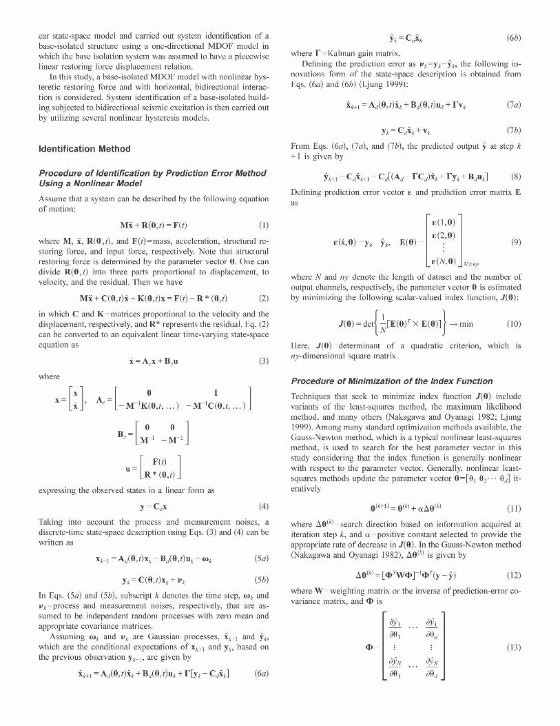
Fig. 1. Outline of multiple shear spring (MSS) model and its skeleton curve characteristics: (a) Single spring; (b) plane view of entire MSS model; (c) perspective diagram of entire MSS model; (d) skeleton curve of a single spring; and (e) skeleton curve of entire MSS model (four springs).
Application of Multiple Shear Spring Model to Nonlinear System
As mentioned earlier, the behavior of base-isolated structures during an earthquake is highly affected by the characteristics of the base isolation system. The base isolation system has two important functions. One is to move the structure's natural frequency away from the dominant frequency range of input excitation, and the other is to dissipate the response kinetic energy. The restoring force of the base isolation system is the combined forces of isolators and energy dissipation devices. Numerous types of devices have been proposed for energy dissipation, where most of them utilize a hysteretic damping mechanism. Therefore, in order to identify a base-isolated structure precisely, having a model, which can represent the nonlinear hysteretic characteristics of the restoring force, is essential.
When the restoring forces of the base isolation system have nonlinear hysteretic characteristics, bidirectional motions in a horizontal plane are coupled together. For example, using a bilinear elastoplastic restoring force model, the yield point is a function of the horizontal strain rather than the movement in the horizontal orthogonal directions. To determine whether the deformation is in the elastic or plastic range should be based on the horizontal strain.
The multiple shear spring (MSS) model (Wada and Kinoshita 1985; Wade and Hirose 1989), which is used in this study, is one of the models which can take into account the nonlinear restoring force as well as the effect of interaction of horizontal displacement components. As shown in Fig. 1, the MSS model is an elastoplastic model consisting of several spaced shear springs, evenly spaced in a circular configuration. Each spring has its own specific characteristic. Fig. 1(d) shows a skeleton curve by a typical bilinear spring. In this case, the characteristics of each spring are determined by initial stiffuess, secondary stiffuess, and yield displacement. When displacements along the north-south (NS) and the east-west (EW) directions are obtained, the deformation and restoring force of each spring can be calculated by using displacement increments along the EW and NS directions as
(l4a)
tlxns = xn/t) - xns(t - 1) (l4b)
where xew(t) and xew(t) = EW and NS displacements at time t. By resolving the restoring force of each spring into the EW
and NS directions and adding up all the restoring force components in each direction, the increments of the total restoring forces along the EW and NS directions can be evaluated by
(15a)
'IT 6 j ="N(i-1) (i=1,2, ... ,N) (l5b)
where tlRew and tlRns = increments of restoring forces along the EW and NS directions, k; (t) = stiffness of ith spring at time t, N =number of shear springs, and 6 j =angle between the EW axis and the ith spring.
The characteristic of each shear spring is determined by the so-called target skeleton curve of the MSS model. Assuming isotropy of the restoring force characteristics in the horizontal plane, yield displacement Uy' and stiffuess k' of each shear spring can be evaluated by the following equations:
N
L cos2 6 j
i~1
Uy' = N Uy (l6a)
L Icos 6 j l
k' = ---:N::----k (l6b)
where Uy and k represent the yield displacement and the stiffness of the target skeleton curve of the MSS model, respectively.
The shape of the skeleton curve of the MSS model under onedirectional deformation is shown in Fig. l(e). In Fig. l(e) the dashed line represents the target skeleton curve and the solid line represents the actual skeleton curve of the MSS model. It should be noted that if we use four springs and each spring has one yield displacement, the MSS model actually has two yield displacements [Fig. 1(e)]. According to the MSS model, when the deformation takes place along the EW direction, the first yield point corresponds to the yield point of spring No.1, while the second yield point corresponds to the yield points of springs No.2 and No.4.
Simulations
To evaluate the effect of initial values of model parameters and measurement noise condition on the performance of the proposed identification technique, a series of computer simulations is conducted. A one-story bidirectional structure model assuming that the restoring force characteristics can be represented by the trilinear hysteretic MSS model is adopted. Mass of the upper structure is specified to be 980,000 kg. Structural response data subject to bidirectional horizontal seismic accelerations of the 1940 El Cen

Table 1. Results of Simulations
Model parameters Exact
(a) Initial values=0.75 times of exact, noise-free
Primary stiffness [kN/cm] 386.9
Secondary stiffness [kN/cm] 116.1
Tertiary stiffness [kN/cm] 77.38
Primary yield displacement [cm] 0.3000
Secondary yield displacement [cm] 2.000
(b) Initial values= 1.25 times of exact, noise-free
Primary stiffness [kN/cm] 386.9
Secondary stiffness [kN/cm] 116.1
Tertiary stiffness [kN/cm] 77.38
Primary yield displacement [cm] 0.3000
Secondary yield displacement [cm] 2.000
(c) Initial values=0.75 times of exact, SNR=0.05
Primary stiffness [kN/cm] 386.9
Secondary stiffness [kN/cm] 116.1
Tertiary stiffness [kN/cm] 77.38
Primary yield displacement [cm] 0.3000
Secondary yield displacement [cm] 2.000
(d) Initial values= 1.25 times of exact, SNR=0.05
Primary stiffness [kN/cm] 386.9
Secondary stiffness [kN/cm] 116.1
Tertiary stiffness [kN/cm] 77.38
Primary yield displacement [cm] 0.3000
Secondary yield displacement [cm] 2.000
Note: SNR =signal-to-noise ratio.
tro earthquake was generated using the linear acceleration method (Chopra 2001) with a time-step of 0.02 s. To quantify the measurement noise condition, signal-to-noise ratio (SNR) is defined as SNR=a~/a; where as and an=signal standard deviation and noise standard deviation, respectively. In the cases of noise contaminated signal condition, zero mean, white uniform noises at a SNR of 0.05 are added to the seismic accelerations and structural responses. In all cases, assuming that the mass of the upper structure is known, primary stiffuess, secondary stiffuess, tertiary stiffness, primary yield displacement, and secondary yield displacement of the target skeleton curve in the MSS model are identified as the model parameters by using the bidirectional ground accelerations as seismic excitation, and the bidirectional relative displacement and velocity responses with respect to the foundation as observation.
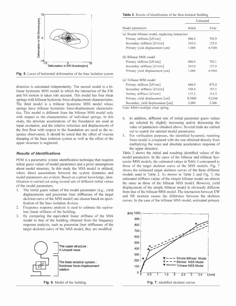
The first case utilized the noise-free signals and the initial values of the model parameters are set to 0.75 times of exact values. System identification took 37 Gauss-Newton iterations to converge with final index function J(O) of 9.6779 X 10-55 • Results of this simulation are presented in Table I (a). The second case utilized the noise-free signals and the initial values of the model parameters are set to I .25 times the exact values. System identification took eight Gauss-Newton iterations to converge with the final index function J(O) of 3.9195 X 10-44 • Results of this simulation are presented in Table I(b). The third case utilized the signals that are contaminated by noise with a SNR of 0.05 and the initial values of the model parameters are set to the same values
Estimated
Initial Final
290.2 386.9
87.05 116.1
58.04 77.38
0.3750 0.3000
1.500 2.000
483.6 386.9
145.1 116.1
96.73 77.38
0.2250 0.3000
2.500 2.000
290.2 377.9
87.05 107.2
58.04 77.44
0.3750 0.3696
1.500 2.063
483.6 445.6
145.1 120A
96.73 77.67
0.2250 0.2611
2.500 1.720
as the first case. System identification took 27 Gauss-Newton iterations to converge with the final index function J(O) of 0.61344. Results of this simulation are presented in Table I(c). The forth and the final case utilized the signals that are contaminated by noise with a SNR of 0.05 and the initial values of the model parameters are set to the same values as the second case. System identification took 22 Gauss-Newton iterations to converge with the final index function J(O) of 0.96362. Results of this simulation are presented in Table l(d).
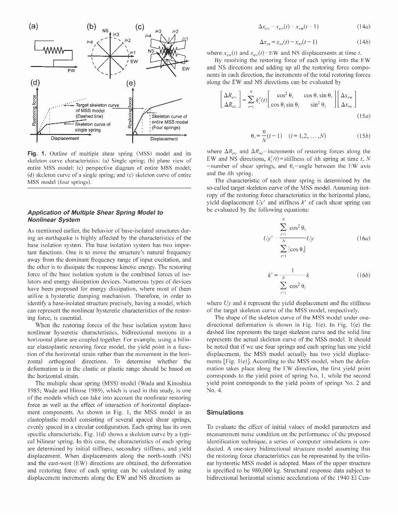
In all four cases, divergence of model parameter values did not occur through the iteration process. In the two cases that utilized the noise-free signals, the final estimated values completely accord with the exact values. In the other two cases that utilized the noise-contaminated signals, the final estimated values converged within the range of relative error 23%. However, the shapes of target skeleton curves obtained by the estimated parameters almost agree with the shapes of the true skeleton curves as shown in Fig. 2. These results support that the proposed technique is able to make reasonably good approximation of nonlinear restoring force characteristics using recorded seismic data. Fig. 3 shows the convergence process of Gauss-Newton iterations in the system identification procedure. Setting of the initial values of the model parameters affects the number of Gauss-Newton iteration and does not affect the accuracy of the estimation. Accuracy of the final estimation and final value of the index function J(O) depends on the noise condition.
I ·.'
234 52 345 Displacement (em) Displacement <em)
Fig. 2. Exact and estimated target skelton curves of the trilinear multiple shear spring model: (a) Initial values=0.75 times of exact, signal-to-noise ratio (SNR)=0.05; and (b) initial values= 1.25 times of exact, SNR=0.05
Identification of Base-Isolated Building
Objective Building and Recordings
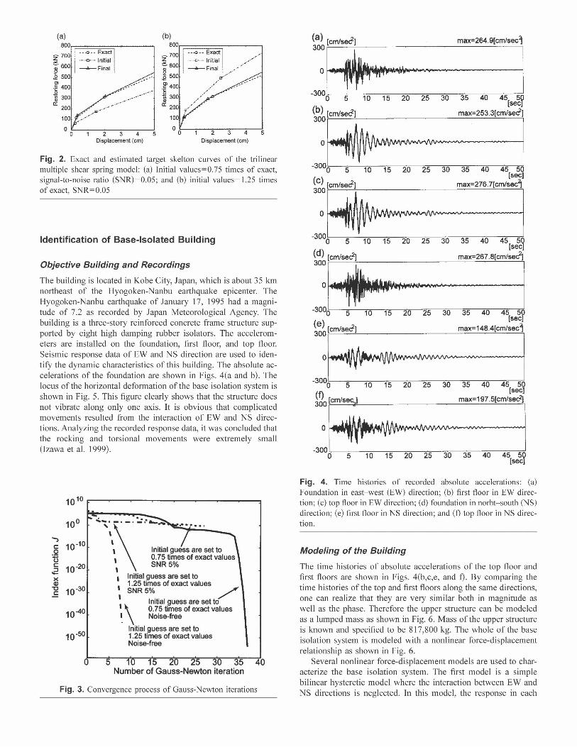
The building is located in Kobe City, Japan, which is about 35 km northeast of the Hyogoken-Nanbu earthquake epicenter. The Hyogoken-Nanbu earthquake of January 17, 1995 had a magnitude of 7.2 as recorded by Japan Meteorological Agency. The building is a three-story reinforced concrete frame structure supported by eight high damping rubber isolators. The accelerometers are installed on the foundation, first floor, and top floor. Seismic response data of EW and NS direction are used to identifY the dynamic characteristics of this building. The absolute accelerations of the foundation are shown in Figs. 4(a and b). The locus of the horizontal deformation of the base isolation system is shown in Fig. 5. This figure clearly shows that the structure does not vibrate along only one axis. It is obvious that complicated movements resulted from the interaction of EW and NS directions. Analyzing the recorded response data, it was concluded that the rocking and torsional movements were extremely small (Tzawa et al. 1999).
10 10 .----.-.......- .........--.--......-....---.-"""":1
. ..
I
'\\-'~~5% Initial guess are set to 1.25 times of exact values
~ SNR5% / Initial guess are set to
I \ 0.75 times of exact values I Noise-free
Initial guess are set to 1.25 times of exact values Noise-free
5 Number of Gauss-Newton iteration
Fig. 3. Convergence process of Gauss-Newton iterations
(a) [cm/sed!j max=264.9[cm/sec1
M:~ -3000 5 10 15 20 25 30 35 40 45[ 50
sec]
\~:~~.2767(am'~1
-3000 5 10 15 20 25 30 35 40 45 50 [sec]
(d) [cm/secf] max=267.8[cm/se<i1]
30:~~. I
-3000 5 10 15 20 25 30 35 40 45 50 [sec]
\~:~4B41'~~~j
-3000 5 10 15 20 25 30 35 40 45 50 [sec]
.:~~o 5 10 15 20 25 30 35 40 45 50
[sec]
Fig. 4. Time histories of recorded absolute accelerations: (a) Foundation in east-west (EW) direction; (b) first floor in EW direction; (c) top floor in EW direction; (d) foundation in norht-south (NS) direction; (e) first floor in NS direction; and (f) top floor in NS direction.
Modeling of the Building
The time histories of absolute accelerations of the top floor and first floors are shown in Figs. 4(b,c,e, and f). By comparing the time histories of the top and first floors along the same directions, one can realize that they are very similar both in magnitude as well as the phase. Therefore the upper structure can be modeled as a lumped mass as shown in Fig. 6. Mass of the upper structure is known and specified to be 817,800 kg. The whole of the base isolation system is modeled with a nonlinear force-displacement relationship as shown in Fig. 6.
Several nonlinear force-displacement models are used to characterize the base isolation system. The first model is a simple bilinear hysteretic model where the interaction between EW and NS directions is neglected. In this model, the response in each
15~----~------,
:[c: o U ~
Ci CIl Z 0 .5 c: o 15 E ~ o
-15,1,.-- _____;;,---------...,-15 0 15
Deformation in EW Direction[cm]
Fig. 5. Locus of horizontal deformation of the base isolation system
direction is calculated independently. The second model is a bilinear hysteretic MSS model in which the interaction of the EW and NS motion is taken into account. This model has four shear springs with bilinear hysteretic force-displacement characteristics. The third model is a trilinear hysteretic MSS model whose springs have trilinear hysteretic force-displacement characteristics. This model is different from the bilinear MSS model only with respect to the characteristics of individual springs. In this study, the absolute accelerations of the foundation are used as input excitation, and the relative velocities and displacements of the first floor with respect to the foundation are used as the response observation. It should be noted that the effect of viscous damping of the base isolation system as well as the effect of the upper structure is neglected.
Results of Identifications
PEM is a parametric system identification technique that requires initial guess values of model parameters and a priori assumptions about model structure. In this study the MSS model is utilized, where direct associations between the system dynamics and model parameters are evident. Based on a priori knowledge, identification is carried out using several sets of different initial values of the model parameters. 1. The initial guess values of the model parameters (e.g., yield
displacements and piecewise liner stiffuesses of the target skeleton curve of the MSS model) are chosen based on specification of the base isolation devices.
2. Frequency response analysis is used to estimate the equivalent linear stiffness of the building.
3. By comparing the equivalent linear stiffness of the MSS model to that of the building obtained from the frequency response analysis, such as piecewise liner stiffuesses of the target skeleton curve of the MSS model, they are modified.
The upper structure: ] A lumped mass
The base isolation system : Nonlinear force-displacement relation]
Table 2. Results of Identification of the Base-Isolated Building
Estimated
Model parameters Initial Final
(a) Simple bilinear model, neglecting interaction Primary stiffness [kN/cm] 686.0 703.9 Secondary stiffness [kN/cm] 343.0 125.0 Primary yield displacement [cm] 1.000 0.5281
(b) Bilinear MSS model Primary stiffness [kN/cm] 686.0 702.1 Secondary sti ffness [kN/cm] 343.0 127.4 Primary yield displacement [cm] 1.000 0.5941
(c) Trilinear MSS model Primary stiffness [kN/cm] 686.0 875.4 Secondary stiffness [kN/cm] 548.8 197.5 Tertiary sti ffness [kN/cm] 137.2 113.3 Primary yield displacement [cm] 0.5000 0.2164 Secondary yield displacement [cm] 2.000 3.366
Note: MSS=multiple shear spring.
4. In addition, different sets of initial parameter guess values are selected by slightly increasing and/or decreasing the value of parameters obtained above. Several trials are carried out to search for optimal model parameters.
5. For verification purposes, the identified hysteretic restoring force model is compared with the one obtained directly from multiplying the mass and absolute acceleration response of the upper structure.
Table 2 shows the initial and resulting identified values of the model parameters. In the cases of the bilinear and trilinear hysteretic MSS models, the estimated values in Table 2 correspond to those of the target skeleton curve of the MSS models. Fig. 7 shows the estimated target skeleton curves of the three different models used in Table 2. As shown in Table 2 and Fig. 7, the estimated stiffuess values of the simple bilinear model are almost the same as those of the bilinear MSS model. However, yield displacement of the simple bilinear model is obviously different from that of the bilinear MSS model. The interaction between EW and NS motions causes the difference between the skeleton curves. In the case of the trilinear MSS model, estimated primary
[kN] 1000 r-----r---r---r--..----,.---r---r-~
900
800
700
600 , ,.. ' , .. '500 , .. '.;':.......400 / ..'
300 4 L ? _. - ._. Simple Bilinear Model
200 v - - - Bilinear MSS Model ~ - Trilinear MSS Model
0.5 1.5 2 2.5 3 3.5 4[cm]
Fig. 6. Model of the building Fig. 7. Identified skeleton curves
3~~Jr-[kNc:!I __--_ 3~~lr-[kc:!NI__--_ ~Jo,r-[k:.:,N],-----_--_
o~ ~ L-- Identified model -- Identified model - Idenbfied model
-3000 Observed data -300 Ob"erved data -3000 Observed data ~ 0 ~ ~ 0 ~ ~ 0 ~
[em] [eml [em]
(d) [kNI (e)[kNI (f) [kNI 3000~'------- 3000 30001~'--------
0 ...'·tfI· / //
-- Identified model --Ideritified model -3000 Observed data -3000 . -3001~=::..>&~""'-'~
-20 0 20 -20 0 20 -20 [eml [eml
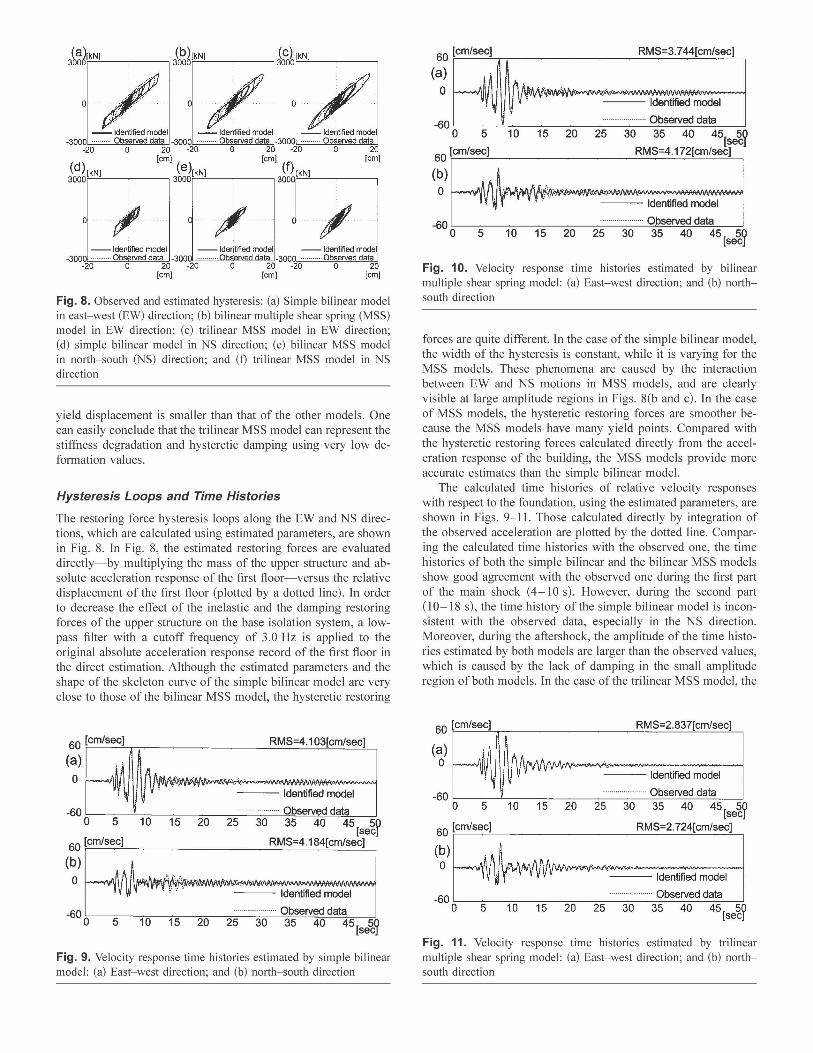
Fig. 8. Observed and estimated hysteresis: (a) Simple bilinear model in east-west (EW) direction; (b) bilinear multiple shear spring (MSS) model in EW direction; (c) trilinear MSS model in EW direction; (d) simple bilinear model in NS direction; (e) bilinear MSS model in north-south (NS) direction; and (t) trilinear MSS model in NS direction
yield displacement is smaller than that of the other models. One can easily conclude that the trilinear MSS model can represent the stiffness degradation and hysteretic damping using very low deformation values.
Hysteresis Loops and Time Histories
The restoring force hysteresis loops along the EW and NS directions, which are calculated using estimated parameters, are shown in Fig. 8. In Fig. 8, the estimated restoring forces are evaluated directly-by multiplying the mass of the upper structure and absolute acceleration response of the first floor-versus the relative displacement of the first floor (plotted by a dotted line). In order to decrease the effect of the inelastic and the damping restoring forces of the upper structure on the base isolation system, a lowpass filter with a cutoff frequency of 3.0 Hz is applied to the original absolute acceleration response record of the first floor in the direct estimation. Although the estimated parameters and the shape of the skeleton curve of the simple bilinear model are very close to those of the bilinear MSS model, the hysteretic restoring
60 [cm/sec] RMS=4.103[cm/sec]
(a)
o 1/V'V'(iIJ··...WJ!",'I'iW'~W<f~-ww.NNvWWlf>JWv""""'~ --- Identified model
-60 ;,-~~--'--::;:;:;------:;-;:-----;;:;:;-----;;:-;:-"_"'_""-:::''':-;:-''''_'''_''~O'g:bse~rv~e~d~d!!=!.at!S!a,=-~ o 5 10 15 20 25 30 35 40 45 50
[sec] 60 [cm/sec] RMS=4.184[cm/sec]
(~) ~"~"~\\lrA,11~lfr!~"~"rW"/"fI,'/:,'~'\v.¥WMPNWVM~I\AAf>M<lM/WlJwwwWWW'~ '1 " --- Identified model
-60 ;'0-'5"..----.1nO-~15;:-----;2~0 ·2"'~;-- ....--'O""3b~5se""rv'-'.ed7.40~d~a~t~~5o-[----=-!50...... ·--;;·;"'·~·-sec]
Fig. 9. Velocity response time histories estimated by simple bilinear model: (a) East-west direction; and (b) north-south direction
60 [cm/sec] RMS=3.744[cm/sec]
(a) o
Identified model
-60 ':-_=----'- ......·__ ...._O=bs~e~rv~ed=d~ata~_...J
o 5 10 15 20 25 30 35 40 45[ 50sec]
60 [cm/sec] RMS=4.172[cm/sec]
--- Identified model
..................... Observed data -60
0 5 10 15 20 25 30 35 40 45[ 50sec]
Fig. 10. Velocity response time histories estimated by bilinear multiple shear spring model: (a) East-west direction; and (b) northsouth direction
forces are quite different. In the case of the simple bilinear model, the width of the hysteresis is constant, while it is varying for the MSS models. These phenomena are caused by the interaction between EW and NS motions in MSS models, and are clearly visible at large amplitude regions in Figs. 8(b and c). In the case of MSS models, the hysteretic restoring forces are smoother because the MSS models have many yield points. Compared with the hysteretic restoring forces calculated directly from the acceleration response of the building, the MSS models provide more accurate estimates than the simple bilinear model.
The calculated time histories of relative velocity responses with respect to the foundation, using the estimated parameters, are shown in Figs. 9-11. Those calculated directly by integration of the observed acceleration are plotted by the dotted line. Comparing the calculated time histories with the observed one, the time histories of both the simple bilinear and the bilinear MSS models show good agreement with the observed one during the first part of the main shock (4-10 s). However, during the second part (l0-18 s), the time history of the simple bilinear model is inconsistent with the observed data, especially in the NS direction. Moreover, during the aftershock, the amplitude of the time histories estimated by both models are larger than the observed values, which is caused by the lack of damping in the small amplitude region of both models. In the case of the trilinear MSS model, the
RMS=2.837[cm/sec]60 [cm/sec]
(a) o
--- Identified model
-60 ':---::----'---:-::---:-=---:0-:----:--=.. ...- .......- - ...--:- .... .. ...::O~b::::se~rv_.:.e~d::..d~a::.::ta~_____.J o 5 10 15 20 25 30 35 40 45 [ 50
sec] 60 [cm/sec) RMS=2.724[cm/sec)
(b) o
--- Identified model
-60 );----_;;-----:;-;:;-----:~-;:;;:;--~-..·-.. ·-;:~ ..·_......·-...._:::O_==bs=e~rv~e::d:...:d::a~ta::_~ o 5 10 15 20 25 30 35 40 45 [ 50
sec]
Fig. 11. Velocity response time histories estimated by trilinear multiple shear spring model: (a) East-west direction; and (b) northsouth direction
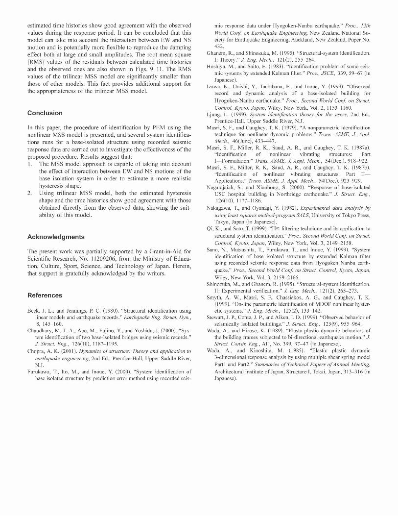
estimated time histories show good agreement with the observed values during the response period. It can be concluded that this model can take into account the interaction between EW and NS motion and is potentially more flexible to reproduce the damping effect both at large and small amplitudes. The root mean square (RMS) values of the residuals between calculated time histories and the observed ones are also shown in Figs. 9-11. The RMS values of the trilinear MSS model are significantly smaller than those of other models. This fact provides additional support for the appropriateness of the trilinear MSS model.
Conclusion
In this paper, the procedure of identification by PEM using the nonlinear MSS model is presented, and several system identifications runs for a base-isolated structure using recorded seismic response data are carried out to investigate the effectiveness of the proposed procedure. Results suggest that: 1. The MSS model approach is capable of taking into account
the effect of interaction between EW and NS motions of the base isolation system in order to estimate a more realistic hysteresis shape.
2. Using trilinear MSS model, both the estimated hysteresis shape and the time histories show good agreement with those obtained directly from the observed data, showing the suitability of this model.
Acknowledgments
The present work was partially supported by a Grant-in-Aid for Scientific Research, No. 11209206, from the Ministry of Education, Culture, Sport, Science, and Technology of Japan. Herein, that support is gratefully acknowledged by the writers.
References
Beck, 1. 1., and Jennings, P. C. (1980). "Structural identification using linear models and earthquake records." Earthquake Eng. Struct. Dyn., 8, 145-160.
Chaudhary, M. T. A., Abe, M., Fujino, Y., and Yoshida, J. (2000). "System identification of two base-isolated bridges using seismic records." 1. Struct. Eng., 126(10), 1187-1195.
Chopra, A. K. (200 I). Dynamics of structure: Theory and application to
earthquake engineering, 2nd Ed., Prentice-Hall, Upper Saddle River, N.J.
Furukawa, T., Ito, M., and Inoue, Y. (2000). "System identification of base isolated structure by prediction error method using recorded seis
mic response data under Hyogoken-Nanbu earthquake." Proc., 12th
World Corif. on Earthquake Engineering, New Zealand National Society for Earthquake Engineering, Auckland, New Zealand, Paper No. 432.
Ghanem, R., and Shinozuka, M. (1995). "Structural-system identification. I: Theory." 1. Eng. Mech., 121(2),255-264.
Hoshiya, M., and Saito, E. (1983). "Identification problem of some seismic systems by extended Kalman filter." Proc., JSCE, 339, 59-67 (in Japanese).
Izawa, K., Onishi, Y., Tachibana, E., and Inoue, Y. (1999). "Observed record and dynamic analysis of a base-isolated building for
Hyogoken-Nanbu earthquake." Proc., Second World Corif. on Struct.
Control, Kyoto, Japan, Wiley, New York, Vol. 2, 1153-1160. Ljung, 1. (1999). System identification theory for the users, 2nd Ed.,
Prentice-Hall, Upper Saddle River, N.J. Masri, S. E, and Caughey, T. K. (1979). "A nonparametric identification
technique for nonlinear dynamic problems." Trans. ASME, J. Appl. Mech., 46(June), 433-447.
Masri, S. E, Miller, R. K., Saud, A. R., and Caughey, T. K. (l987a). "Identification of nonlinear vibrating structures: Part I~Formulation." Trans. ASME, 1. Appl. Mech., 54(Dec.),918-922.
Masri, S. F., Miller, R. K., Saud, A. R., and Caughey, T. K. (l987b). "Identification of nonlinear vibrating structures: Part II~
Applications." Trans. ASME, 1. Appl. Mech., 54(Dec.), 923-929. Nagarajaiah, S., and Xiaohong, S. (2000). "Response of base-isolated
USC hospital building in Northridge earthquake." 1. Struct. Eng., 126(10),1177-1186.
Nakagawa, T., and Oyanagi, Y. (1982). Experimental data analysis by
using least squares method-program SALS, University of Tokyo Press, Tokyo, Japan (in Japanese).
Qi, K., and Sato, T. (1999). "Hoo filtering technique and its application to
structural system identification." Proc., Second World Con! on Struct. Control, Kyoto, Japan, Wiley, New York, Vol. 3, 2149-2158.
Sano, N., Matsushita, T., Furukawa, T., and Inoue, Y. (1999). "System identification of base isolated structure by extended Kalman filter using recorded seismic response data from Hyogoken Nanbu earth
quake." Proc., Second World Corif. on Struct. Control, Kyoto, Japan,
Wiley, New York, Vol. 3, 2159-2166. Shinozuka, M., and Ghanem, R. (1995). "Structural-system identification.
II: Experimental verification." 1. Eng. Mech., 121(2),265-273. Smyth, A. W., Masri, S. E, Chassiakos, A. G., and Caughey, T. K.
(1999). "On-line parametric identification of MDOF nonlinear hysteretic systems." 1. Eng. Mech., 125(2), 133-142.
Stewart, J. P., Conte, J. P., and Aiken, 1. D. (1999). "Observed behavior of seismically isolated buildings." 1. Struct. Eng., 125(9), 955-964.
Wada, A., and Hirose, K. (1989). "Elasto-plastic dynamic behaviors of the building frames subjected to bi-directional earthquake motion." 1. Struct. Constr. Eng., AIl, No. 399, 37-47 (in Japanese).
Wada, A., and Kinoshita, M. (1985). "Elastic plastic dynamic 3-dimensional response analysis by using multiple shear spring model
Part1 and Part2." Summaries of Technical Papers ofAnnual Meeting,
Architectural Institute of Japan, Structure I, Tokai, Japan, 313-316 (in Japanese).