IT Licentiate theses2012-007

System identification and controlfor general anesthesia based onparsimonious Wiener models

MARGARIDA MARTINS DA SILVA

UPPSALA UNIVERSITYDepartment of Information Technology

System identification and control

for general anesthesia based onparsimonious Wiener models

Margarida Martins da Silva����������������� ���

October 2012

Division of Systems and ControlDepartment of Information Technology

Uppsala UniversityBox 337

SE-751 05 UppsalaSweden

�������������� ����

Dissertation for the degree of Licentiate of Philosophy in Electrical Engineering with

Specialization in Automatic Control

c© Margarida Martins da Silva 2012

ISSN 1404-5117

Printed by the Department of Information Technology, Uppsala University, Sweden

Abstract

The effect of anesthetics in the human body is usually describedby Wiener models. The high number of patient-dependent parame-ters in the standard models, the poor excitatory pattern of the inputsignals (administered anesthetics) and the small amount of availableinput-output data make application of system identification strategiesdifficult.

The idea behind this thesis is that, by reducing the number of pa-rameters to describe the system, improved results may be achieved whensystem identification algorithms and control strategies based on thosemodels are designed. The choice of the appropriate number of parame-ters matches the parsimony principle of system identification.

The three first papers in this thesis present Wiener models with areduced number of parameters for the neuromuscular blockade and thedepth of anesthesia. Batch and recursive system identification algo-rithms are presented. Taking advantage of the small number of continu-ous time model parameters, adaptive controllers are proposed in the twolast papers. The controller structure combines an inversion of the staticnonlinearity of the Wiener model with a linear controller for the exactlylinearized system, using the parameter estimates obtained recursively byan extended Kalman filter. The performance of the adaptive nonlinearcontrollers is tested in a database of realistic patients with good results.

2

Acknowledgments

First of all, I would like to thank my supervisors for their support,guidance and inspiration, and for always being available for discussionswhenever I needed them. Each one of my supervisors had a specialcontribution to my life during these years. Teresa Mendonca showed methat medicine can be fun. Torbjorn Wigren accepted me as an externalstudent in Uppsala back in 2009 (that made the difference!) and trustedme while working independently. Alexander Medvedev taught me thatresearch has its ”outdoor” side.

The administrative staff of the department deserve a thanks for allthe help and service they provided, specially because a great part of thathad to be done through emails.

Thanks also to all friends and colleagues at the Division of Systemsand Control in Uppsala, and all the GALENO group in Porto. Researchdoes not make any sense without team work.

I would like to express my gratitude to the Fundacao para a Cienciae a Tecnologia for the research grant SFRH/BD/60973/2009, and also tothe European Research Council (Advanced Grant 247035) for partiallyfunding the work done in this thesis. Fundacao Calouste Gulbenkian,Fundacao Luso-Americana para o Desenvolvimento and Bernt JarmarksFoundation also contributed financially to this work, which is gratefullyacknowledged.

A special thanks go to my parents, Catarina and Reinhard for un-conditional support and love all along the PhD, and for accepting thatI cannot be physically present in Portugal, Austria and Sweden at thesame time.

3

4

List of Papers

This thesis is based on the following papers:

I M. M. Silva, T. Wigren, and T. Mendonca. Nonlinear identificationof a minimal neuromuscular blockade model in anesthesia. IEEETransactions on Control Systems Technology, vol. 20, no. 1, pp.181-188, Jan. 2012.

II M. M. Silva, T. Mendonca, and T. Wigren. Online nonlinear iden-tification of the effect of drugs in anaesthesia using a minimal pa-rameterization and BIS measurements. In Proc. American ControlConference (ACC’10), Baltimore, Maryland, pp. 4379-4384, Jun.30-Jul. 2, 2010.

III M. M. Silva. Prediction error identification of minimally parame-terized Wiener models in anesthesia. In Proc. 18th IFAC WorldCongress, Milan, Italy, pp. 5615-5620, Aug. 28-Sep. 2, 2011.

IV M. M. Silva, T. Mendonca, and T. Wigren. Nonlinear adaptivecontrol of the neuromuscular blockade in anesthesia. In Proc. 50thIEEE Conference on Decision and Control and European ControlConference (CDC-ECC’11), Orlando, Florida, pp. 41-46, Dec. 12-15, 2011.

V M. M. Silva, T. Wigren, and T. Mendonca. Exactly linearizingadaptive control of propofol and remifentanil using a reducedWienermodel for the depth of anesthesia, to appear in Proc. 51st IEEEConference on Decision and Control (CDC’12), Maui, Hawaii, Dec.10-13, 2012.

5

6

Contents

1 Introduction 9

1.1 General anesthesia at a glance . . . . . . . . . . . . . . . . 9

1.2 Drug delivery in anesthesia: standard practice . . . . . . . 11

1.3 Challenges . . . . . . . . . . . . . . . . . . . . . . . . . . . 11

1.4 Thesis contributions . . . . . . . . . . . . . . . . . . . . . 13

1.5 Outline . . . . . . . . . . . . . . . . . . . . . . . . . . . . 13

2 Standard models in anesthesia 15

2.1 Neuromuscular blockade . . . . . . . . . . . . . . . . . . . 16

2.1.1 Linear dynamics . . . . . . . . . . . . . . . . . . . 16

2.1.2 Static nonlinearity . . . . . . . . . . . . . . . . . . 17

2.2 Depth of anesthesia . . . . . . . . . . . . . . . . . . . . . . 18

2.2.1 Linear dynamics . . . . . . . . . . . . . . . . . . . 18

2.2.2 Static nonlinear interaction . . . . . . . . . . . . . 19

3 Automatic drug delivery in anesthesia 21

3.1 Neuromuscular blockade . . . . . . . . . . . . . . . . . . . 21

3.2 Depth of anesthesia . . . . . . . . . . . . . . . . . . . . . . 22

4 Nonlinear system identification 25

4.1 Overview . . . . . . . . . . . . . . . . . . . . . . . . . . . 26

4.1.1 Modeling paradigms . . . . . . . . . . . . . . . . . 26

4.1.2 System identification methods . . . . . . . . . . . . 27

4.2 Nonlinear model structures . . . . . . . . . . . . . . . . . 28

4.3 The Wiener model structure . . . . . . . . . . . . . . . . . 32

4.3.1 Input signals . . . . . . . . . . . . . . . . . . . . . 33

4.3.2 System identification algorithms . . . . . . . . . . 34

7

5 Nonlinear adaptive control for Wiener systems 395.1 Overview . . . . . . . . . . . . . . . . . . . . . . . . . . . 395.2 Linearization by inversion . . . . . . . . . . . . . . . . . . 405.3 Linear controller design . . . . . . . . . . . . . . . . . . . 41

5.3.1 Pole placement . . . . . . . . . . . . . . . . . . . . 415.3.2 Linear quadratic Gaussian control . . . . . . . . . 43

5.4 Antiwindup . . . . . . . . . . . . . . . . . . . . . . . . . . 45

6 Included Papers 47

Bibliography 50

8

Chapter 1

Introduction

1.1 General anesthesia at a glance

General anesthesia is a reversible drug-induced loss of consciousness dur-ing which patients are not arousable, even by painful stimulation. Pa-tients under anesthesia often require assistance in maintaining a patentairway because of depressed spontaneous ventilation or drug-induceddepression of the neuromuscular function [3].

This definition embodies the three main components of general anesthe-sia: hypnosis, analgesia and muscle relaxation. In order to achieve agood compromise of these three components, anesthesiologists admin-ister several drugs, while simultaneously maintaining all the vital func-tions of the patient within acceptable ranges.

Hypnosis is related to unconsciousness and to the inability of the pa-tient to recall intraoperatory events. The drugs mostly related to theloss of consciousness are hypnotics. Since hypnotics alter electrocorti-cal activity in a dose-dependent manner [60], it has been assumed thatthe electroencephalographic activity is informative enough to be usedas a surrogate measurement of hypnosis [22]. Some of the electroen-cephalogram (EEG)-derived indices that are commercially available arethe Index of Consciousness (IoC) [33], the Spectral Entropy (SE) [77],and the Bispectral Index (BIS) [18]. The BIS is the most widely usedindex to infer the hypnosis of a patient. This is the major reason whyit is used for the research work presented in this thesis. It is related

9

to the responsiveness level and the probability of intraoperative recalland it ranges from 0 (equivalent to the absence of brain activity) to 97.7(representing a fully awake and alert state) in a dimensionless continu-ous scale. Values between 40 to 60 indicate an adequate BIS level forgeneral anesthesia [34].

Analgesia is associated with pain relief. During general anesthesia, theconscious experience of pain disappears due to hypnosis. There is how-ever some activity, denoted nociception [66], generated in the peripheraland central nervous system as a result of stimuli that has the poten-tial to damage tissues. The physiological effects of nociception, togetherwith the hormonal and catabolic changes that accompany surgery (sur-gical stress response), can be attenuated with analgesics [36]. In spiteof several trials to quantify the level of analgesia in anesthetized pa-tients [29, 11], direct indicators of the extension of analgesia are not yetcommercially available. Hence, the estimation of the analgesia level bythe anesthesiologists is commonly based on unspecific autonomic reac-tions, such as changes in the blood pressure and heart rate, sweating,pupil reactivity and the presence of tears [25]. A source of complexityin this system is that some of these clinical responses might be partiallysuppressed by the effect of muscle relaxants.

Most of the hypnotics and analgesics interact in such a way that theireffect is enhanced when administered together [54, 78, 51]. This is thereason why, in most of the cases, the term Depth of Anesthesia (DoA)is used to assess the joint hypnosis and analgesia of a patient.

Muscle relaxation aims to ease the patients’ intubation, to facilitatethe access to internal organs, and to avoid movement responses as aresult of surgical stimuli. The neuromuscular blockade (NMB) is usuallymeasured from one evoked muscle response at the hand of the patientsubject to electrical stimulation of the adductor pollicis muscle throughsupra maximal train-of-four (TOF) stimulation of the ulnar nerve, andit can be registered by electromyography (EMG), mechanomyography(MMG) or acceleromyography (AMG) [47]. In the TOF mode, the NMBcorresponds to the first single response (T1) calibrated by a referencetwitch, ranging between 100% (full muscular activity) and 0% (completeparalysis). Among the research community, the EMG is the preferredmeasure for the NMB because it is easy to apply and less vulnerable tomechanical interferences [68].

10

1.2 Drug delivery in anesthesia: standard prac-tice

In the current anesthesia practice, anesthetics are administered followingstandard dosing guidelines, often based on the average patient [9]. Asit stands, the inter (and intra) patient variability in the dose-responserelationship is not directly considered. The common procedure is toadminister the initial dose of anesthetics as suggested in the guidelines,observe the response, and adjust the dose accordingly, also taking intoaccount the clinical environment and the surgical protocols that are be-ing followed. The titration process to reach an individualized dose isdone by trial and error [9], and highly depends on the anesthesiologist’sunderstanding of both the pharmacokinetics (PK) and the pharmacody-namics (PD) of the drugs in use, as well as the possible drugs interaction.It has been seen that the use of the knowledge of the anesthetics PK/PDas an additional input to the anesthesiologists’ decisions results in im-proved patient care [6]. The anesthesiologist hence acts as a feedbackcontroller.

The natural question here is whether automatic controllers, using themodels for the anesthetics disposition and effect, are able to overcomethe need for individualization, further improving the complex decisionof drug delivery in anesthesia.

1.3 Challenges

Several of the core features of drug delivery in anesthesia constitute ma-jor challenges for the development of automatic closed-loop controllers.

First of all, the patients’ PK/PD responses are nonlinear and time-varying. The nonlinear nature results from a sigmoidal relationship be-tween the drug concentration at the effect site and the observed effect.The time-varying profile is mainly the consequence of several noxiousstimulation, the change in the tolerance to drugs, unmodeled interac-tions between drugs or other major changes in the patient (e.g. bloodlosses) that may occur during a general anesthesia procedure [70]. Con-sequently, models should preferably be established individually and inreal-time [79].

11

Another considerable challenge for the development of automatic drugdelivery platforms in anesthesia is the nonnegative nature of the sys-tem. This constraint also needs to be accounted for. Since no drugscan be removed from the patients once administered, the variables to becontrolled (drugs rates) are intrinsically nonnegative. Moreover, all thesyringe pumps that are available in the market impose an upper limitin the drug rate they can administer. This can be tackled by introduc-ing actuator nonlinearities. If not accounted for in the control design,the system can become unstable. These effects are clear for adaptivecontrollers which continue to adapt even when the system is saturated,leading to windup effects and unacceptable transients after saturation[26].

The limited amount of real-time data and the poor excitation propertiesof the input signals constitute further fundamental challenges. These arethe two major reasons that triggered and justified the development ofthe research work presented in this thesis. On one hand, at the begin-ning of a general anesthesia procedure, when no substantial data fromthe patient is available, the knowledge about the individual PK/PD ofthe patients is insufficient to initialize and tune the control algorithms.On the other hand, due to the monitoring devices or other restrictionsfrom the clinical protocol, the sampling frequency of the signals of in-terest is far from ideal and usually quite slow. Moreover, due to medicalconstraints, the inputs are not allowed to be chosen for best performanceof identification experiments [79]. These reasons, together with the highnumber of parameters in the physiologically-based PK/PD models thatare commonly used for the dynamics of drugs in anesthesia, motivatethe use of low-complexity models [75, 27].

From the reasons stated above, it is reasonable to assume that, by reduc-ing the number of parameters to describe the system, improved resultsmay be achieved when system identification and control algorithms aredesigned. The choice of the appropriate number of parameters shouldmatch the parsimony principle of system identification [72], that looselystates that the ”best” model to describe a certain system should containthe smallest number of free parameters required to represent the truesystem adequately.

12

1.4 Thesis contributions

The first contribution of this thesis is the modeling of the dispositionand effect of some of the most commonly used anesthetics in the clinicalpractice (the muscle relaxant atracurium, the hypnotic propofol and theanalgesic remifentanil) using Wiener models with very few free parame-ters. The second contribution is the development of batch and recursivesystem identification methods for the identification of the parametersin the new models. Identification of continuous time parameters is per-formed due to the desire to keep the number of identified parametersat a minimum. The result is a continuous time model, which is easilydiscretized. Hence, both continuous time and discrete time controllersynthesis is easily applied. The third contribution is the use of thepreviously developed reduced Wiener models and identification strate-gies in nonlinear adaptive controllers for both the NMB and the DoA.The last contribution is the assessment of the controllers performanceas evaluated over a database of simulated realistic patients.

1.5 Outline

This thesis is divided into two major blocks. The first block gives anoverview of both the biomedical application and the engineering toolsneeded to understand and to position the research of this thesis in thegeneral framework. Chapter 2 describes the standard PK/PD modelsthat are most commonly used to describe the drug-effect relationship ofmuscle relaxants, hypnotics and analgesics. These are not the modelsused for the controller development in this thesis but motivate the needfor models with few parameters in this application. Chapter 3 presentsthe state of the art in automatic drug delivery in anesthesia. Chapter 4deals with nonlinear system identification and modeling, while chapter 5introduces the nonlinear adaptive control techniques for Wiener systemsthat are used in this thesis. The choice of the controller framework wasdefined by the application in hand. Chapter 6 summarizes the includedpapers. The second block consists of reprints of the papers resultingfrom the research performed for this licentiate.

13

14

Chapter 2

Standard models inanesthesia

The standard physiologically-based models describing the relationshipbetween the administered anesthetic dose and its effect may be dividedinto four cascaded blocks [52]. The first one relates the dose of anestheticwith its blood plasma concentration. This constitutes the PK model ofthe drug. The second block relates the concentration of the drug in theblood plasma with the effect concentration i.e the concentration of thedrug on its site of effect: in the case of muscle relaxants, the neuromuscu-lar junction; and in the case of hypnotics and analgesics, the brain. Thethird block describes the relationship between the effect concentrationand the observed effect. The second and third steps constitute the PDmodel of the drug. In the case of simultaneous administration of severaldrugs, a fourth block may be present representing the PD interactionbetween drugs.

In what the PK is concerned, the distribution of the drugs in the bodydepends on several transport and metabolic processes. Compartmentalmodels [24] capture this behavior by considering the body divided incompartments that exchange positive amounts of drugs between eachother. Assuming an instantaneous mixing of the drug in each compart-ment, conservation laws are used to derive the associated dynamic equa-tions. Two or three compartmental (mammilary) models are the onesmost commonly used to describe the PK of muscle relaxants, hypnoticsand analgesics.

15

Since the blood plasma is not the effect site of any of the anesthetics,a delay between the concentrations of the drugs and observed effectexists. The indirect link models [15] model this delay by connecting anadditional virtual effect compartment, clinically assumed with negligiblevolume to ensure that the equilibrium of the PK is not affected, to thecentral (plasma) compartment. This constitutes the linear part of thePD model.

At the effect site, the way anesthetics act has a more involving character-ization than the distribution of the anesthetics in the body. Empiricalmodels are therefore used to describe this part of the PD [15]. Theclassic and most commonly used is the Hill function, a sigmoid staticnonlinear function relating the effect concentration of the drug with itsobserved effect.

Given this, the dose-effect relationship of muscle relaxants, hypnoticsand analgesics may be seen as Wiener models: linear dynamics followedby a static nonlinearity (Fig. 4.2(b)).

2.1 Neuromuscular blockade

2.1.1 Linear dynamics

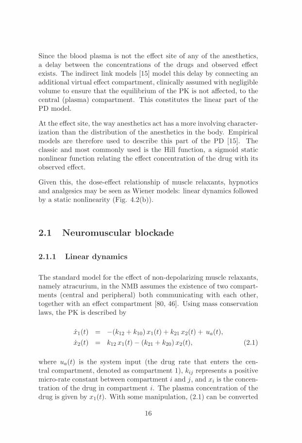
The standard model for the effect of non-depolarizing muscle relaxants,namely atracurium, in the NMB assumes the existence of two compart-ments (central and peripheral) both communicating with each other,together with an effect compartment [80, 46]. Using mass conservationlaws, the PK is described by

x1(t) = −(k12 + k10)x1(t) + k21 x2(t) + ua(t),

x2(t) = k12 x1(t)− (k21 + k20)x2(t), (2.1)

where ua(t) is the system input (the drug rate that enters the cen-tral compartment, denoted as compartment 1), kij represents a positivemicro-rate constant between compartment i and j, and xi is the concen-tration of the drug in compartment i. The plasma concentration of thedrug is given by x1(t). With some manipulation, (2.1) can be converted

16

to the macro-constants state-space representation

x1(t) = −λ1 x1(t) + a1 ua(t),

x2(t) = −λ2 x2(t) + a2 ua(t), (2.2)

cp(t) =

2∑i=1

xi(t),

relating the administered muscle relaxant rate ua(t) [μg kg−1min−1] with

its plasma concentration cp(t) [μg ml−1]. xi(t), {i=1,2} are state vari-ables (implicitly defined by (2.2)), and ai [kg ml−1], λi [min−1], {i=1,2}are patient-dependent parameters.

The plasma concentration cp(t) of the muscle relaxant and its effectconcentration ce(t) [μg ml−1] are related by the linear PD as

c(t) = −λ c(t) + λcp(t), (2.3)

ce(t) = −1/τ ce(t) + 1/τ c(t), (2.4)

where c(t) is an intermediate variable, and λ [min−1] and τ [min] arepatient-dependent parameters.

The standard models developed for atracurium [80] do not consider (2.4).As shown in [38], the inclusion of this equation, corresponding to a firstorder approximation of the τ delay, allows a better replication of theobserved experimental responses.

2.1.2 Static nonlinearity

The PD nonlinearity relates the effect concentration ce(t), impossible tomeasure in the clinical practice, to the effect of the drug as quantified bythe measured NMB y(t) [%]. It is usually modeled by the Hill function[80] as

y(t) =100Cγ

50

Cγ50 + cγe (t)

, (2.5)

where C50 [μg ml−1] and γ (dimensionless) are also patient-dependentparameters.

The total number of parameters in the NMB standard model character-izing each individual patient response is hence eight.

17

2.2 Depth of anesthesia

2.2.1 Linear dynamics

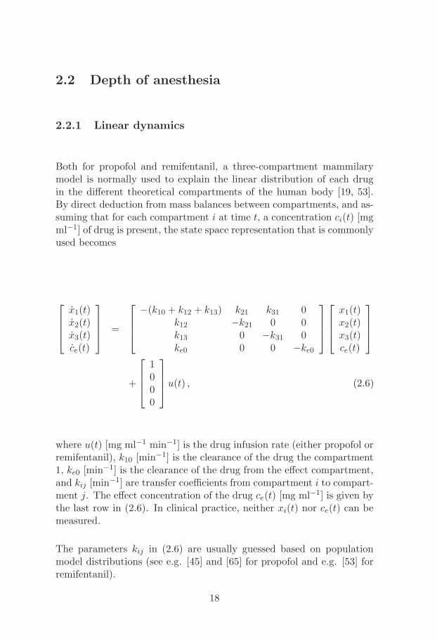
Both for propofol and remifentanil, a three-compartment mammilarymodel is normally used to explain the linear distribution of each drugin the different theoretical compartments of the human body [19, 53].By direct deduction from mass balances between compartments, and as-suming that for each compartment i at time t, a concentration ci(t) [mgml−1] of drug is present, the state space representation that is commonlyused becomes

⎡⎢⎢⎣

x1(t)x2(t)x3(t)ce(t)

⎤⎥⎥⎦ =

⎡⎢⎢⎣

−(k10 + k12 + k13) k21 k31 0k12 −k21 0 0k13 0 −k31 0ke0 0 0 −ke0

⎤⎥⎥⎦

⎡⎢⎢⎣

x1(t)x2(t)x3(t)ce(t)

⎤⎥⎥⎦

+

⎡⎢⎢⎣

1000

⎤⎥⎥⎦u(t) , (2.6)

where u(t) [mg ml−1 min−1] is the drug infusion rate (either propofol orremifentanil), k10 [min−1] is the clearance of the drug the compartment1, ke0 [min−1] is the clearance of the drug from the effect compartment,and kij [min−1] are transfer coefficients from compartment i to compart-ment j. The effect concentration of the drug ce(t) [mg ml−1] is given bythe last row in (2.6). In clinical practice, neither xi(t) nor ce(t) can bemeasured.

The parameters kij in (2.6) are usually guessed based on populationmodel distributions (see e.g. [45] and [65] for propofol and e.g. [53] forremifentanil).

18

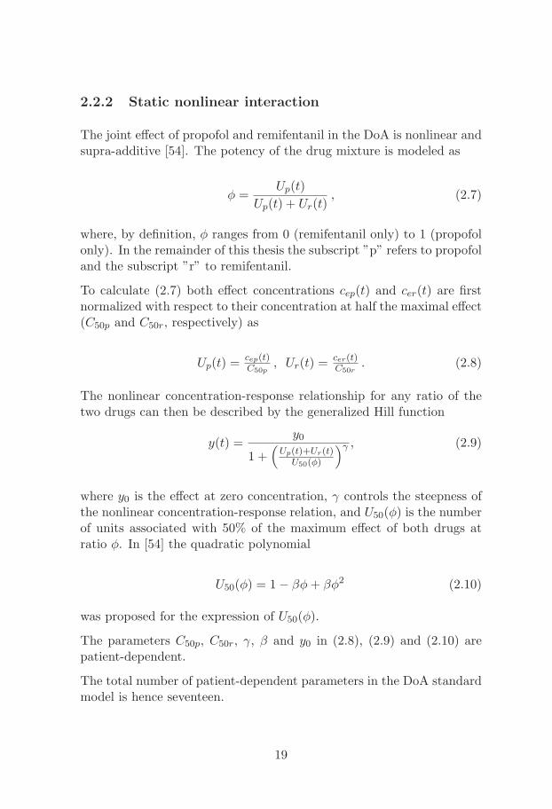
2.2.2 Static nonlinear interaction

The joint effect of propofol and remifentanil in the DoA is nonlinear andsupra-additive [54]. The potency of the drug mixture is modeled as

φ =Up(t)

Up(t) + Ur(t), (2.7)

where, by definition, φ ranges from 0 (remifentanil only) to 1 (propofolonly). In the remainder of this thesis the subscript ”p” refers to propofoland the subscript ”r” to remifentanil.

To calculate (2.7) both effect concentrations cep(t) and cer(t) are firstnormalized with respect to their concentration at half the maximal effect(C50p and C50r, respectively) as

Up(t) =cep(t)C50p

, Ur(t) =cer(t)C50r

. (2.8)

The nonlinear concentration-response relationship for any ratio of thetwo drugs can then be described by the generalized Hill function

y(t) =y0

1 +(Up(t)+Ur(t)

U50(φ)

)γ , (2.9)

where y0 is the effect at zero concentration, γ controls the steepness ofthe nonlinear concentration-response relation, and U50(φ) is the numberof units associated with 50% of the maximum effect of both drugs atratio φ. In [54] the quadratic polynomial

U50(φ) = 1− βφ+ βφ2 (2.10)

was proposed for the expression of U50(φ).

The parameters C50p, C50r, γ, β and y0 in (2.8), (2.9) and (2.10) arepatient-dependent.

The total number of patient-dependent parameters in the DoA standardmodel is hence seventeen.

19

20

Chapter 3

Automatic drug delivery inanesthesia

The need to individualize the drug delivery to patients undergoing gen-eral anesthesia is clear and acknowledged by the medical community[74].

3.1 Neuromuscular blockade

The conventional procedure to provide muscle relaxation to patients un-dergoing anesthesia is the administration of bolus doses i.e. impulses ofshort duration aiming to induce a quick drop in the NMB level. Thesize of the bolus is estimated according to the patient’s weight, followingthe drugs dosing guidelines and taking into account the type of anesthe-sia and surgical protocol that is being performed. This procedure givesconsiderable fluctuations in the levels of relaxation [39]. Moreover, sincemost of the muscle relaxants have high therapeutic indices in hospitalsettings, they are often used in excess of minimal effective requirements[20]. This overdosing eliminates fine control of the NMB and may in-crease the incidence of side-effects. In this context, closed-loop controlof muscle relaxant administration appears as a beneficial option. Be-sides avoiding overdosing, the achievement of a better regulation of theNMB also enables a more meaningful evaluation of patient’s depth ofanesthesia [16].

21

The initial studies on closed-loop control of muscle relaxants date backto the 80’s [12, 61, 31]. Mainly due to the fact that the system is sin-gle input single output with reliable sensors available, the NMB settinghas been considered ideal for the initial development and performanceassessment of several different drug delivery strategies since then. Nev-ertheless, none of these control strategies are wide spread in the dailyclinical practice. Proportional-integral-derivative (PID) controllers areamong the ones most extensively developed. In [57], vecuronium ad-ministration was controlled by a four-phase PID with good results evenunder unstable surgical conditions. The software Hipocrates [49] thathas been used mainly for atracurium constitutes an important contri-bution to the individualization of muscle relaxant delivery. Switchingtechniques were also tried [48]. In [2] a hybrid method was proposedto identify the parameters of the standard PK/PD model using datafrom the initial bolus response. In an identification error-free case, anasymptotic convergence of the NMB to the reference is guaranteed bythe inversion of the static gain of the linear part of the model, coupled tothe inverse of the nonlinearity. For mivacurium, a model-based adaptivegeneralized predictive controller was proposed and tested in [32] withgood results. The ”Rostocker assistant system for anesthesia control(RAN)”, besides controlling the NMB, also includes a module to controlthe depth of hypnosis. This prototype shows the potential of mergingthe control of the NMB and the DoA in a single platform.

3.2 Depth of anesthesia

The first successful attempt to automatically attain a predefined indi-vidualized concentration of anesthetics in the central (plasma) or effectcompartment was the so-called target-controlled infusion (TCI). Whileusing TCI-based devices, initially developed for the hypnotic propofol[23], the anesthesiologist is able to set the desired theoretical (target)concentration of the drug, and the device calculates, in an open-loopfashion, the amount of drug that will target that specific concentration.In spite of the control laws being proprietary, it is known that theyare based on published population models for the PK/PD of the drugs,where the patient’s height, age, weight and gender are used as covariatesto calculate the model parameters in (2.6). For the hypnotic propofol,TCI devices incorporating two adult models are commercial available:

22

the Marsh [45] and the Schnider [65] model. For the opioid remifentanil,the Minto model [53] is the one implemented.

Even though enabling a quicker and more accurate achievement of thetarget theoretical effect concentration than standard manual adminis-tration protocols [74], there still exists some inacurracy in the patients’dose-effect relationship that is not covered by the linear PK/PD models(see section 2.2.1). This means that the TCI technologies need an ac-tive role from the anesthesiologist to titrate the ”adequate” target effectconcentration for each patient, based on all the monitored physiologicalsignals and measurements from the patient. Therefore the loop is onlypartially closed by the anesthesiologist. It is not the measured effectthat is the input for the controller (i.e. the anesthesiologist), but oneestimate of the intermediate signal (i.e. the effect concentration) in theWiener structure.

A crucial question here is why closed-loop strategies have not beenwidely implemented and accepted in the daily clinical use? There aremany reasons for this: a) the physiological processes behind anesthe-sia are not well enough understood yet; b) the inter and intra patientvariability is high. It has e.g. been shown that models that hold foradults do not perform well when applied to elderly or children [1]; c) thelack of reliable and direct sensors to quantify the hypnosis and analgesiaprevent automatic control; d) maybe the most relevant, the ethical andlegal terms concerning even supervised closed-loop control of DoA areextensive since malfunction of the controller can be lethal.

Consequently, it is not surprising that closed-loop (individualized) con-trol in anesthesia has been a topic of intense discussion and research dur-ing the last years. The common goal of all approaches is to contributeto the development of a decision support system, aiming at improvingthe patients’ safety in the clinical setting.

Adaptive control and robust control to model uncertainties are two tech-niques often implemented to overcome the inter and intra patient vari-ability in the response to the administration of hypnotics and analgesics.For example, [13] presents a direct adaptive controller for uncertain lin-ear nonnegative dynamical systems, applied to propofol administrationin anesthesia, where the relationship between the effect concentrationand the measured effect was considered as a fixed linear static function.This assumption might however be too restrictive since the input-output

23

relationship for propofol follows a nonlinear Wiener model behavior. Onthe other hand, [30] presents a comparison between a robust predic-tive control strategy, the EPSAC [55], and a Bayesian-based closed loopsystem [70], showing the applicability of the predictive controllers in areal-life environment.

Several works constitute hybrid solutions of adaptive and robust control.In [73] the controller is inherently a PID where the parameters of thePD and the time delay are identified during the induction period. Thisstrategy shows good results when applied to a database of 44 simulatedpatients. The performance of this strategy might however worsen whenthe dynamics of the drug distribution or effect change during the anes-thetic procedure. Also for propofol administration, the model-predictivesetting in [63] assumes that the PK of the patient given by the standardmodel in [67] is always correct, while the PD parameters and dead-timeare identified by least squares during the induction phase.

While in the previously referred works propofol was used as the singlecontrolled input, [50] and [37] are examples of studies where the influ-ence of remifentanil in the DoA control was taken into account in afeedforward fashion. This option stands as an intermediate step to afully automatic drug delivery system for intravenous anesthesia.

As a further step forward, [40] and [17] present two closed-loop con-trollers for DoA using propofol and remifentanil as controlled inputs.The core of the algorithm in [40] is the widely used TCI concept. Theloop is closed by empirical rules which define new effect concentrationsetpoints for the two drugs depending on the error between the mea-sured and the target BIS. In this case, no individualized control strategyis applied. The mismatch between the observed and predicted systemresponses is overcome by changing the control target. Even thoughempirical, this strategy gives good results when validated over a pop-ulation of 83 patients. Robustness to major patient dynamics changeswas not assessed. Similarly, [17] keeps the PK parameters of propofoland remifentanil fixed, identifying the PD parameters in the interactionbetween the two drugs and dead times. By introducing a new analgesiaindex, results in this work seem promising. However, the authors ac-knowledge that the identification of patient individual parameters hasto be improved.

24

Chapter 4

Nonlinear systemidentification

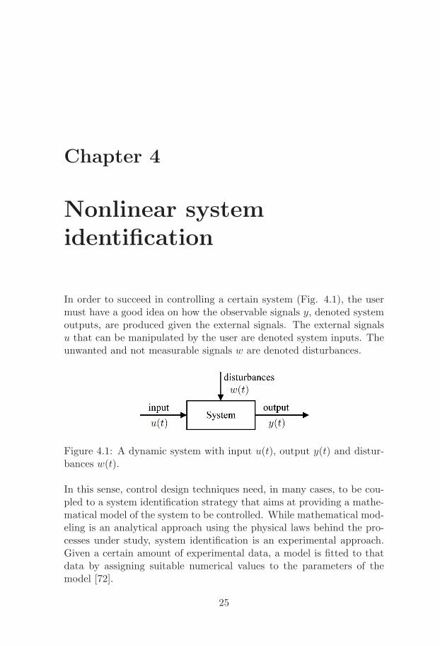
In order to succeed in controlling a certain system (Fig. 4.1), the usermust have a good idea on how the observable signals y, denoted systemoutputs, are produced given the external signals. The external signalsu that can be manipulated by the user are denoted system inputs. Theunwanted and not measurable signals w are denoted disturbances.

Figure 4.1: A dynamic system with input u(t), output y(t) and distur-bances w(t).

In this sense, control design techniques need, in many cases, to be cou-pled to a system identification strategy that aims at providing a mathe-matical model of the system to be controlled. While mathematical mod-eling is an analytical approach using the physical laws behind the pro-cesses under study, system identification is an experimental approach.Given a certain amount of experimental data, a model is fitted to thatdata by assigning suitable numerical values to the parameters of themodel [72].

25

Due to the generality of system identification, its range of applicationsspans from industrial and chemical processes to medicine and economy.The nonlinear dynamics of many of the systems, e.g. pH control andvalves [5], flight dynamics [28], processes in wastewater treatment plants[44] or temperature control for solar furnaces [14], make the developmentof system identification techniques for those systems a demanding task.

Initially, classical control methods were designed with stability in mind[10]. Experimental tests for the tuning of the controller were usuallyrequired to assess its robustness. Consequently, the system variation un-der uncertainties could only be considered if those uncertain conditionswould persist from one experiment to the other. By utilizing moderncontrol design techniques, the uncertainty of a system due to variancewithin the plant can be directly calculated, and the tradeoff betweenperformance and stability can be displayed graphically. This ability al-lows modern controllers to perform over a wider range of conditions, andsupports the need for the development of models for the design. Thesemodels can e.g. be obtained by system identification experiments.

4.1 Overview

4.1.1 Modeling paradigms

Depending on how much a priori information is used in the model, themodeling of a system can be classified as white-box, gray-box or black-box.

In white-box modeling, the model is fully derived from the physical lawsbehind the process. In this case, all the a priori information about thesystem dynamics is used to derive the model. One useful property ofthe white-box models is that the values of the model parameters havea physical meaning that can e.g. be compared with tabled values forthose quantities.

On the contrary, in black-box modeling, no a priori information is used toestablish a model, which is strictly based on the collected input-outputdata. The main advantage of this reasoning is that the obtained modelsare, in most of the cases, of low complexity. The drawback is that thereis little or no connection between the obtained parameter values and

26

the physical entities involved in the process. Note that the selection ofa model structure that is needed to perform black-box modeling is somekind of prior information. Such models are considered black-box despiteof the model selection.

A compromise between the two previous modeling paradigms is gray-boxmodeling. Since some a priori information about the system is used, theresulting models are semi-physical [42].

In spite of which paradigm is used to model a certain system, a choicehas to be made on whether the model should be formulated in discreteor continuous time. Discrete time models (or difference equations) areusually used to describe events for which it is natural to look at thesystem and collect data at fixed (discrete) intervals. Continuous timemodels, on the other hand, provide a description of the continuous timesystem. This might be of interest for nonlinear systems since most non-linear control theory is based on continuous time models [35].

Due to the fact that the dynamics of anesthetics in the human bodyis nonlinear, and to enable a broader choice of controllers, the modelsproposed in this thesis are formulated in continuous time.

4.1.2 System identification methods

Recursive vs. batch

Recursive identification refers to algorithms where the estimated param-eters are updated every time a new observation of the system is avail-able. Typically, the new estimate is equal to the previous estimate plus acorrection term which depends on the prediction error. Recursive identi-fication schemes are useful when the system dynamics are time-varying.A further advantage of recursive identification is that the requirementon computational memory is quite modest since not all data are stored.

Batch identification, in opposition, uses all the available data at once tocreate the ”best” model for the system [41].

27

Parametric vs. nonparametric

Parametric methods can be seen as mappings from the recorded data to afinite-dimensional estimated parameter vector. Examples of parametricmethods are prediction error methods and subspace methods [41].

Nonparametric methods provide models that are curves, tables or func-tions that do not (explicitly) result from a finite-dimensional parame-ter vector. Impulse responses, frequency diagrams or series expansionsthrough kernels (like Volterra and Wiener series expansions) are exam-ples of models obtained with such methods. Examples of nonparametricmethods are transient analysis and spectral analysis [72].

4.2 Nonlinear model structures

This section gives an overview of some of the most commonly used non-linear model structures.

Series expansions

Using the Volterra operator

Hn[u(t)] =

∫ ∞

−∞. . .

∫ ∞

−∞hn(σ1, . . . , σn)u(t− σ1) . . . u(t− σn) dσ1 . . . dσn,

(4.1)the output y(t) can be described as a functional series expansion of theinput signal u(t) [64] as

y(t) = h0 +∞∑n=1

Hn[u(t)]. (4.2)

In a system identification framework, the objective is to find the Volterrakernel hn(σ1, . . . , σn) for σi = 0, σ1

i , . . . , σNii , {i = 1, . . . , n}, where Ni

is the number of points in which each σi is evaluated, assuming a discretetime setup.

Since the Volterra system representation is an infinite series, it is onlymeaningful if convergence is guaranteed. Moreover, computing the Volte-rra series given a certain input-output data is not an easy task due to the

28

vast amount of parameters and the coupling in between them. Wienerproposed a series representation that has certain orthogonality proper-ties with respect to the statistical characterization of the response [62],

y(t) =

∞∑n=0

Gn[kn, u(t)], (4.3)

where the Wiener functionals Gn[kn, u(t)] are orthogonal for a whiteGaussian noise input. Consequently, the Wiener kernels kn(σ1, . . . , σn)can then be easily separated, which makes the identification easier. How-ever, the high number of unknown parameters and the whiteness restric-tion on the noise are major drawbacks of these methods.

Discrete time nonlinear difference equations

A nonlinear generalization of the auto regressive moving average withexogenous inputs (ARMAX) model

A(q−1)y(t) = B(q−1)u(t) + C(q−1)e(t) (4.4)

is the nonlinear ARMAX (NARMAX) model

y(t) = F (y(t−1), . . . , y(t−ny), u(t−1), . . . , u(t−nu), e(t−1), . . . , e(t−ne)),(4.5)

where y(t) is the output; u(t) is the input; e(t) is white noise; q−1 is thebackward shift operator; A(q−1), B(q−1) and C(q−1) are polynomialsand F (.) is an arbitrarily nonlinear function.

Similarly, the NARX and NFIR models are the nonlinear equivalents ofARX and FIR models, respectively (see e.g. [69]).

Neural networks

A neural network, which name is inspired on the structure of the humancentral nervous system, is a mathematical model consisting of severalelements, called nodes, arranged in layers. Each node in one layer isconnected to all nodes in the adjacent layers. The choice of a suit-able network architecture can be done by applying methods of modelassessment and selection, such as cross-validation. Once the architec-ture considered to be the best is selected, the corresponding network

29

is trained i.e. a set of values for the network weights are obtained bysolving an optimization problem based on the error between the modeland the collected data. After this offline step, the resulting network canbe applied to new data in order to obtain an estimate of the unknownparameterization. The major drawback of this structure for the identifi-cation is that the number of parameters increases considerably with thenumber of nodes.

Nonlinear ordinary differential equation models

One recently advocated model is an ordinary differential equation (ODE)model parameterized with coefficients of a multi-variable polynomialthat describes one component of the right-hand side function of theODE [83]. The system is formulated in continuous time and in statespace as

x(t) = f(x, u, θ),

y(t) = C x(t), (4.6)

where y(t) is the system output; u(t) is the system input; x(t) is thestate of the system; f(.) is a nonlinear function; and θ is the unknownparameter vector.

If a discrete time model is needed instead, an intuitive way of discretiz-ing the system is to substitute the differential operator by a differenceapproximation [21]. Considering a sampling period T , the Euler forwarddiscretization scheme becomes

x(t+ T ) = x(t) + T f(x, u, θ),

y(t) = C x(t). (4.7)

The disadvantage of the use of an Euler integration scheme is the re-quirement of a fast sampling, a fact that can cause ill-conditioned iden-tification problems.

Bayesian estimation

In the Bayesian approach, the model parameters are inferred through theobservation of random processes that are correlated with the parameters.

30

The approach is related to linear and nonlinear state estimation (”fil-tering”) problems. The Kalman filter (KF) and the extended Kalmanfilter (EKF) are well known examples. The unobserved state vector isassumed to be correlated with the output of the system. Consequently,based on observations of the output, the value of the state vector canbe estimated. While the KF is optimal for linear systems with Gaus-sian inputs, the EKF is not optimal in estimating the state of nonlinearsystems (see section 4.3.2).

The Bayesian approach is useful e.g. when the dynamics of the system ischanging and tracking is required through parameter adaptation. Thisis achieved by modeling also the parameter vector as a random process[43].

Block-oriented models

Block-oriented models exploit the interaction between linear time-inva-riant (LTI) dynamic subsystems and static nonlinear elements [7]. Theseblocks may be interconnected in different ways e.g. series, parallel orfeedback, which makes the block-oriented models flexible enough to cap-ture the dynamics of many real systems.

The simplest structures are composed by two blocks in series.

If the nonlinearity is present at the input, the model is denoted a Ham-merstein model (Fig. 4.2(a)). A list of examples where Hammersteinmodels are used can be found in [7]. Existing methods in the lit-erature for identifications of Hammerstein models comprise the over-parameterization method, stochastic methods, frequency domain meth-ods, and iterative methods (see e.g. [8]).

If the nonlinearity is present at the output, the model is of Wiener type(Fig. 4.2(b)). Cases where there exists saturation in the sensors thatmeasure the system output are usually treated as Wiener models [82].Even though apparently similar, it is easier to perform system identifica-tion in the Hammerstein model than in the Wiener model. The reason isthat the Hammerstein model can be reparameterized as a linear multipleinput single output (MISO) model by a suitable choice of parameteriza-tion [59]. The overparameterization method takes advantage of exactlythis property. The Wiener model structure will be treated in more detailin section 4.3.

31

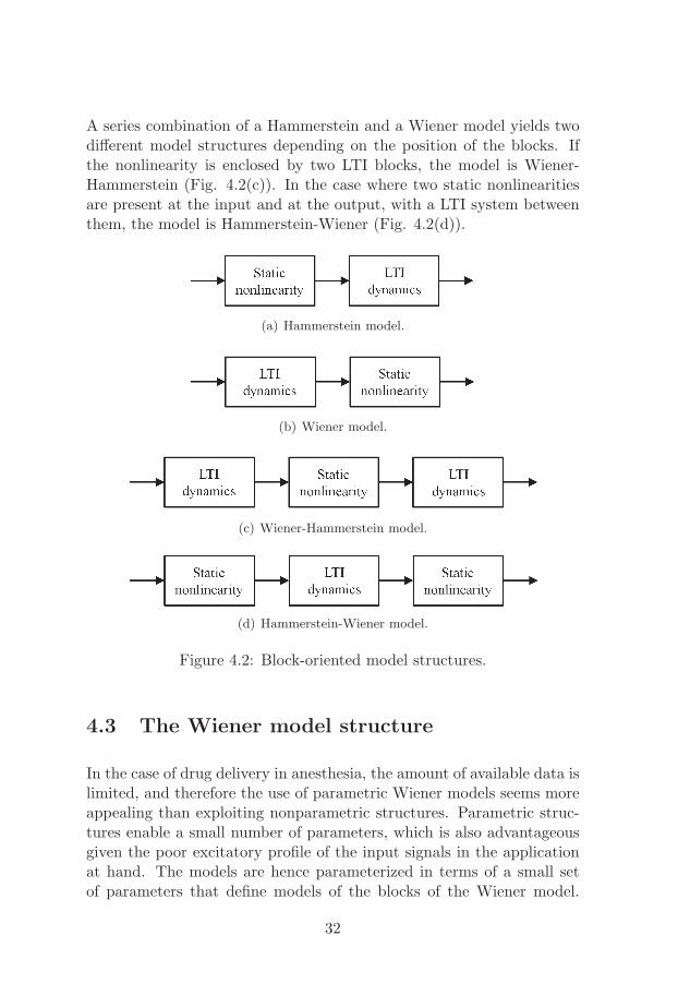
A series combination of a Hammerstein and a Wiener model yields twodifferent model structures depending on the position of the blocks. Ifthe nonlinearity is enclosed by two LTI blocks, the model is Wiener-Hammerstein (Fig. 4.2(c)). In the case where two static nonlinearitiesare present at the input and at the output, with a LTI system betweenthem, the model is Hammerstein-Wiener (Fig. 4.2(d)).

(a) Hammerstein model.

(b) Wiener model.

(c) Wiener-Hammerstein model.

(d) Hammerstein-Wiener model.

Figure 4.2: Block-oriented model structures.

4.3 The Wiener model structure

In the case of drug delivery in anesthesia, the amount of available data islimited, and therefore the use of parametric Wiener models seems moreappealing than exploiting nonparametric structures. Parametric struc-tures enable a small number of parameters, which is also advantageousgiven the poor excitatory profile of the input signals in the applicationat hand. The models are hence parameterized in terms of a small setof parameters that define models of the blocks of the Wiener model.

32

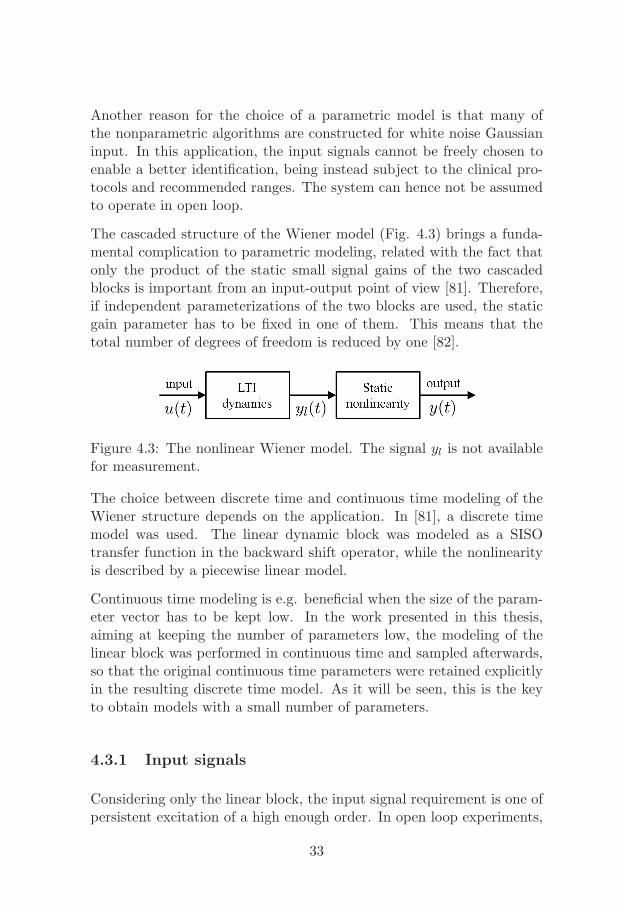
Another reason for the choice of a parametric model is that many ofthe nonparametric algorithms are constructed for white noise Gaussianinput. In this application, the input signals cannot be freely chosen toenable a better identification, being instead subject to the clinical pro-tocols and recommended ranges. The system can hence not be assumedto operate in open loop.

The cascaded structure of the Wiener model (Fig. 4.3) brings a funda-mental complication to parametric modeling, related with the fact thatonly the product of the static small signal gains of the two cascadedblocks is important from an input-output point of view [81]. Therefore,if independent parameterizations of the two blocks are used, the staticgain parameter has to be fixed in one of them. This means that thetotal number of degrees of freedom is reduced by one [82].

Figure 4.3: The nonlinear Wiener model. The signal yl is not availablefor measurement.

The choice between discrete time and continuous time modeling of theWiener structure depends on the application. In [81], a discrete timemodel was used. The linear dynamic block was modeled as a SISOtransfer function in the backward shift operator, while the nonlinearityis described by a piecewise linear model.

Continuous time modeling is e.g. beneficial when the size of the param-eter vector has to be kept low. In the work presented in this thesis,aiming at keeping the number of parameters low, the modeling of thelinear block was performed in continuous time and sampled afterwards,so that the original continuous time parameters were retained explicitlyin the resulting discrete time model. As it will be seen, this is the keyto obtain models with a small number of parameters.

4.3.1 Input signals

Considering only the linear block, the input signal requirement is one ofpersistent excitation of a high enough order. In open loop experiments,

33

the necessary order of persistent excitation equals the number of pa-rameters to be estimated [41]. Regarding the nonlinear block, the inputsignal has to be such that the output of the linear block has energy inall amplitudes where accurate modeling is required [82].

4.3.2 System identification algorithms

Prediction error algorithms

Recalling that a model represents a way of predicting the behavior ofa certain system, an intuitive way to determine the ”best” model for acertain process is to use a measure based on the prediction error [72],

ε(t, θ) = y(t)− y(t|t− 1; θ), (4.8)

where y(t) is the measured output; and y(t|t− 1; θ) is the prediction ofy(t) given the data up to and including t − 1, and based on the modelparameter vector θ.

The performance of the predictor is hence assessed by minimizing acertain prediction error based criterion like

VN (θ) =1

N

N∑t=1

l(t, θ, ε(t, θ)), (4.9)

where l(t, θ, ε) is a scalar-valued (typically positive) function [41] of themodel parameter vector θ.

The estimate θN yielding the ”best” model is hence given by

θN = argminθ

VN (θ). (4.10)

For nonlinear systems, the search for the minimum is usually performednumerically, based on the negative gradient of the prediction error (4.8).In the case of the prediction error method (PEM) [72], this search isdone in batch. The online counterpart of the PEM is the recursive PEM(RPEM) [72]. Examples of the RPEM for nonlinear Wiener models in-clude [81, 56]. The recursive scheme has the advantage of providingupdates of the parameters in time, useful in e.g. adaptive control sys-tems where the time-varying parameters are used in the time-varyingregulator [5].

34

Extended Kalman filter

The idea of the EKF is to use the ideas of the KF for nonlinear models.

The nonlinear discrete time model is given by [71],

x(t+ 1) = f(t, x(t), u(t)) + g(t, x(t))v(t),

y(t) = h(t, x(t)) + e(t), (4.11)

where v(t) and e(t) are mutually independent Gaussian white noise se-quences with zero mean and covariances R1(t) and R2(t), respectively;u(t) is the input signal; and f(.) and h(.) are nonlinear functions.

The model is expanded in a first-order Taylor series around estimatesof the state x(t). The function f(.) is then expanded around the mostrecent estimate x(t|t) as

f(t, x(t), u(t)) ≈ f(t, x(t|t), u(t)) + F (t)(x(t)− x(t|t)), (4.12)

with

F (t) =∂f(t, x, u)

∂x

∣∣∣∣x=x(t|t)

. (4.13)

The output function is expanded around the predicted state x(t|t − 1)as

h(t, x(t)) ≈ h(t, x(t|t− 1) +H(t)(x(t)− x(t|t− 1), (4.14)

with

H(t) =∂h(t, x)

∂x

∣∣∣∣x=x(t|t−1)

. (4.15)

The noise function is evaluated at x(t|t) asg(t, x(t)) ≈ G(t), (4.16)

withG(t) = g(t, x)|x=x(t|t) . (4.17)

Using the previous approximations, the system can be treated with lineartechniques, exploiting the state space model

x(t+ 1) = F (t)x(t) +G(t)v(t) + u(t),

y(t) = H(t)x(t) + e(t) + w(t),

u(t) = f(t, x(t|t), u(t))− F (t)x(t|t), (4.18)

w(t) = h(t, x(t|t− 1))−H(t)x(t|t− 1).

35

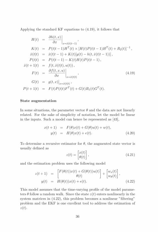
Applying the standard KF equations to (4.19), it follows that

H(t) =∂h(t, x)

∂x

∣∣∣∣x=x(t|t−1)

,

K(t) = P (t|t− 1)HT (t)× [H(t)P (t|t− 1)HT (t) +R2(t)]−1 ,

x(t|t) = x(t|t− 1) +K(t)[y(t)− h(t, x(t|t− 1))] ,

P (t|t) = P (t|t− 1)−K(t)H(t)P (t|t− 1) ,

x(t+ 1|t) = f(t, x(t|t), u(t)) ,F (t) =

∂f(t, x, u)

∂x

∣∣∣∣x=x(t|t)

, (4.19)

G(t) = g(t, x)∣∣x=x(t|t) ,

P (t+ 1|t) = F (t)P (t|t)F T (t) +G(t)R1(t)GT (t).

State augmentation

In some situations, the parameter vector θ and the data are not linearlyrelated. For the sake of simplicity of notation, let the model be linearin the inputs. Such a model can hence be represented as [43],

x(t+ 1) = F (θ)x(t) +G(θ)u(t) + w(t),

y(t) = H(θ)x(t) + e(t). (4.20)

To determine a recursive estimator for θ, the augmented state vector isusually defined as

z(t) =

[x(t)θ(t)

], (4.21)

and the estimation problem uses the following model

z(t+ 1) =

[F (θ(t))x(t) +G(θ(t))u(t)

θ(t)

]+

[wx(t)wθ(t)

],

y(t) = H(θ(t))x(t) + e(t). (4.22)

This model assumes that the time-varying profile of the model parame-ters θ follow a random walk. Since the state z(t) enters nonlinearly in thesystem matrices in (4.22), this problem becomes a nonlinear ”filtering”problem and the EKF is one excellent tool to address the estimation ofz(t).

36

In comparison with other recursive identification techniques, the EKFenables independent tuning using the covariance matrix of both the pro-cess and the measurement noise, thereby giving rise to an independenttuning of the convergence speed for each one of the parameters. Thiswas the main reason for the choice of the EKF to recursively estimatethe parameters of the models presented in this thesis.

37

38

Chapter 5

Nonlinear adaptive controlfor Wiener systems

This chapter gives the technical background for the development of non-linear adaptive controllers for the NMB and the DoA.

The main purpose for the introduction of adaptivity is to handle interand intra patient variability in an improved way. The benefit would bean increased control performance during anesthesia. From the clinicalperspective, robustness of the control is also very important. Adaptivecontrol provides some robustness, by adaptation to individual patientdynamics. However, a systematic study of this, as well as of robustcontrol techniques is a subject for future research.

5.1 Overview

Generally speaking, an adaptive control system can be seen as havingtwo loops [5]. One loop is a normal feedback with the process and thecontroller, and the other loop is the parameter adjustment loop. Aschematic representation of an adaptive controller is shown in Fig. 5.1.

There are two ways of bringing adaptivity to the structures. Eitherthe parameters of the model are estimated, and the control parametersare updated indirectly via the estimation of the process model (indirectadaptive algorithm), or the model can be reparameterized such that the

39

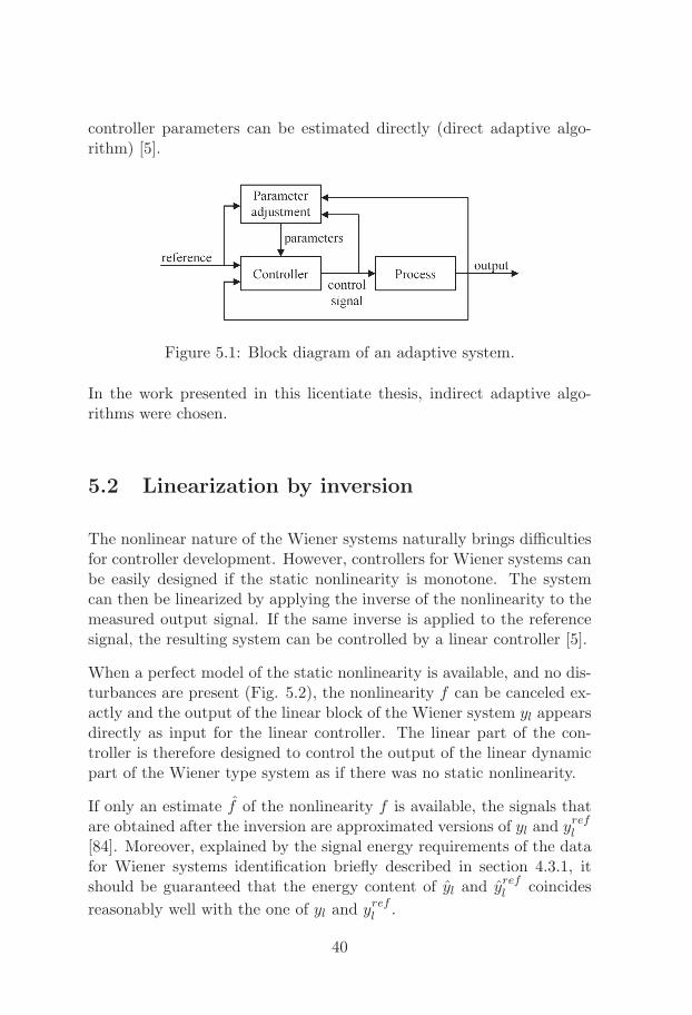
controller parameters can be estimated directly (direct adaptive algo-rithm) [5].

Figure 5.1: Block diagram of an adaptive system.

In the work presented in this licentiate thesis, indirect adaptive algo-rithms were chosen.

5.2 Linearization by inversion

The nonlinear nature of the Wiener systems naturally brings difficultiesfor controller development. However, controllers for Wiener systems canbe easily designed if the static nonlinearity is monotone. The systemcan then be linearized by applying the inverse of the nonlinearity to themeasured output signal. If the same inverse is applied to the referencesignal, the resulting system can be controlled by a linear controller [5].

When a perfect model of the static nonlinearity is available, and no dis-turbances are present (Fig. 5.2), the nonlinearity f can be canceled ex-actly and the output of the linear block of the Wiener system yl appearsdirectly as input for the linear controller. The linear part of the con-troller is therefore designed to control the output of the linear dynamicpart of the Wiener type system as if there was no static nonlinearity.

If only an estimate f of the nonlinearity f is available, the signals thatare obtained after the inversion are approximated versions of yl and yrefl

[84]. Moreover, explained by the signal energy requirements of the datafor Wiener systems identification briefly described in section 4.3.1, itshould be guaranteed that the energy content of yl and yrefl coincides

reasonably well with the one of yl and yrefl .

40

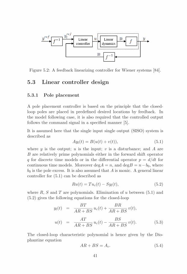
Figure 5.2: A feedback linearizing controller for Wiener systems [84].

5.3 Linear controller design

5.3.1 Pole placement

A pole placement controller is based on the principle that the closed-loop poles are placed in predefined desired locations by feedback. Inthe model following case, it is also required that the controlled outputfollows the command signal in a specified manner [5].

It is assumed here that the single input single output (SISO) system isdescribed as

Ayl(t) = B(u(t) + v(t)), (5.1)

where y is the output; u is the input; v is a disturbance; and A areB are relatively prime polynomials either in the forward shift operatorq for discrete time models or in the differential operator p = d/dt forcontinuous time models. Moreover degA = n, and degB = n−b0, whereb0 is the pole excess. It is also assumed that A is monic. A general linearcontroller for (5.1) can be described as

Ru(t) = Tuc(t)− Syl(t), (5.2)

where R, S and T are polynomials. Elimination of u between (5.1) and(5.2) gives the following equations for the closed-loop

yl(t) =BT

AR+BSuc(t) +

BR

AR+BSv(t),

u(t) =AT

AR+BSuc(t)− BS

AR+BSv(t). (5.3)

The closed-loop characteristic polynomial is hence given by the Dio-phantine equation

AR+BS = Ac. (5.4)

41

The design parameter is the polynomial Ac, chosen such that the closed-loop system has the desired performance. The polynomials R and S canbe determined by solving (5.4). In order to determine T in (5.4), afurther restriction is added. It is required that the response from thecommand signal uc to the output be described by

Amym(t) = Bmuc(t). (5.5)

It then follows from (5.3) that

BT

AR+BS=

BT

Ac=

Bm

Am(5.6)

must hold. The polynomial B is typically factored as

B = B+B−, (5.7)

where B+ is a monic polynomial whose zeros are stable, and well dampedso that they can be canceled by the controller, and B− has the unstableor poorly damped zeros that cannot be canceled. If follows that B−

must be a factor of Bm as

Bm = B−B′m, (5.8)

and B+ must be a factor of Ac, since it is canceled. It also followsfrom (5.6) that Am must be a factor of Ac. Given this, the closed-looppolynomial must have the form

Ac = AoAmB+. (5.9)

Due to the fact that B+ is a factor of B and Ac, it follows from theDiophantine equation that it also divides R. Thus R = B+R′, and theDiophantine equation (5.4) becomes

AR′ +B−S = AoAm = A′c. (5.10)

The polynomial T can hence be obtained by introducing (5.7), (5.8) and(5.9) into (5.6),

T = A0B′m. (5.11)

Conditions on how to obtain a controller that is causal in discrete time(or proper in the continuous time case) can be found in [5, pp.95-96].

The addition of integral action in the controller aims to regulate awayany static error that may be present in the controlled signal y(t). This

42

static error regulation is captured by assuming that the disturbance w(t)in (5.1) is generated by Ad(p)w(t) = e(t), where e(t) is white noise. Interms of pole placement controller design in continuous time, this meansthat an additional stable closed-loop pole X = p+x0 has to be added tothe adaptive controller structure [5, pp.124]. The new polynomial R0(p)will be given by R0 = AdR

0′ . Hence, if R and S are solutions to (5.10),R0 and S0 given by

R0 = XR+ Y B, (5.12)

S0 = XS − Y A, (5.13)

will satisfy [5, pp.123],

AR0 +BS0 = XAc. (5.14)

From (5.12) it follows that

R0 = pR0′ = (p+ x0)R+ y0B, (5.15)

with x0 to be chosen and Y = y0 obtained by making p = 0 in (5.15):

y0 = −x0R(0)

B(0). (5.16)

Inserting X and y0 into (5.12) and (5.13) the new controller is found.The complete control law is then given by

R0u(t) = Tuc(t)− S0yl(t). (5.17)

5.3.2 Linear quadratic Gaussian control

Linear quadratic Gaussian (LQG) control is a tool to deal with linear sys-tems with Gaussian disturbances, through minimization of a quadraticcriterion [71].

The system is given by

x(t+ 1) = Fx(t) +Gu(t) + v(t),

y(t) = Hx(t) + e(t), (5.18)

43

where v(t) and e(t) are jointly Gaussian white noise sequences of zeromean and

E

[v(t)e(t)

] [vT (t) eT (t)

]=

[R1 R12

R12 R2

], (5.19)

where E denotes the expectation operator, and R2 > 0.

The criterion function is often selected as

l =∞∑

t=t0

[xT (t) uT (t)

] [Q1 Q12

Q21 Q2

] [x(t)u(t)

], (5.20)

where the symmetric weighting matrices satisfy [71, pp. 319],

Q2 > 0 and

[Q1 Q12

Q21 Q2

]≥ 0.

The regulator that minimizes the expected loss E l is

u(t) = −L(t)x(t). (5.21)

The matrix L(t) is obtained by solving the discrete-time Ricatti equation[71].

In case of systems with incomplete state information, the optimal per-formance is obtained by substituting the exact state by the optimalstate estimate x(t|t − 1) of (5.18). Even in the presence of arbitrarilydistributed disturbances, the regulator (5.21) is still optimal [71].

When a reference signal uc(t) has to be followed without any static error,the feedback law (5.21) is substituted by

u(t) = −Lx(t) +Muc(t). (5.22)

The appropriate value of M to yield zero static error in the closed loopsystem is

M =[H(I − F +GL)−1G

]−1. (5.23)

Static errors can also be avoided by using integral feedback. For that,an augmented state z(t) =

∑t−1s=0[y(s)− uc(s)] is added to the dynamic

model (5.18). The state space vector becomes x(t) =[xT (t) zT (t)

]and

the augmented model is

x(t+ 1) =

[F 0H I

]x(t) +

[G0

]u(t) +

[0−I

]uc(t). (5.24)

44

The penalty matrix Q1 has to be transformed accordingly as

Q1 =

[Q1 00 Q3

]. (5.25)

The LQG controller for the system in (5.24) becomes

u(t) = −Lx(t)

= −L1x(t)− L2z(t) (5.26)

= −L1x(t)− L2

t−1∑s=0

[y(s)− uc(s)].

The size of the penalty matrix Q3 affects the strength of the integratingterm in the controller.

Faster servo responses on changes of the reference signal can be obtainedby introducing a direct term from uc(t) in (5.26) as

u(t) = −L1x(t)− L2

t−1∑s=0

[y(s)− uc(s)] + L2uc(t). (5.27)

5.4 Antiwindup

The problem of controlling a Wiener system with a monotone nonlinear-ity would be solved with the techniques previously described if no actu-ator saturations existed. However, in most of the real control systems,the actuators have a working range that should be taken care of whiledesigning the controller, because the feedback will be broken wheneverthe actuator saturates. The effects of this saturation are specially visiblewith controller or processes that are unstable, or with controllers withintegral action. If an integrator is included in the design, it winds up(i.e. continues integrating the error) whenever the actuator is saturated.The output of the integrator can then assume very large values, and itcan take a long time to get it back to a normal value again [4]. Thissaturation phenomenon is usually called ”reset windup” or ”integratorsaturation” [4].

Broadly speaking, there are two possible approaches to deal with windupschemes [76]. On the one-step approach, the antiwindup is included in

45

the controller design from the very beginning. The controller hence aimsat ensuring all performance specifications, while handling the saturationconstraints by the actuator. The other possibility is to separate thedesign of the controller and the design of the antiwindup compensator.The controller does not take into account the saturation constraintsand it is designed to ensure that stability is maintained. It is onlywhen saturation occurs that the antiwindup scheme is turned on. Theidea in e.g. [58] is to change the dynamics of the closed-loop systemwhen actuators saturate, so that a good transient behavior is obtainedafter desaturation, while avoiding limit cycles oscillations and repeatedsaturations.

In the pole placement design, the windup is overcome by feeding back theactual process input (saturated) instead of the unsaturated (calculated)input signal. If the controller in (5.2) is written in observer form as

Aou(t) = Tuc(t)− Syl(t) + (Ao −R)u(t), (5.28)

and the saturating actuator is described by the nonlinear function f(.),the controller that avoids windup is then given by [5],

Aov(t) = Tuc(t)− Syl(t) + (Ao −R)u(t),

u(t) = f(v(t)). (5.29)

46

Chapter 6

Included Papers

In this chapter a summary of the papers included in the second partof the thesis is given. Note that the papers have been written to beunderstood separately and therefore some information is repeated.

Paper I

M. M. Silva, T. Wigren, and T. Mendonca. Nonlinear identification ofa minimal neuromuscular blockade model in anesthesia. IEEE Transac-tions on Control Systems Technology, vol. 20, no. 1, pp. 181-188, Jan.2012.

A new SISO Wiener model with two parameters is proposed for the ef-fect of atracurium in the NMB. An EKF is developed to perform theonline identification of the system parameters. This approach outper-forms many conventional identification strategies, and shows good re-sults regarding parameter identification and measured signal tracking,when evaluated on a large patient database. The new method provedto be adequate for the description of the system, even with the poorinput signal excitation and the few measured data samples present inthis application. The method is of general validity for the identificationof drug dynamics in the human body.

47

Paper II

M. M. Silva, T. Mendonca, and T. Wigren. Online nonlinear identifi-cation of the effect of drugs in anaesthesia using a minimal parameter-ization and BIS measurements. In Proc. American Control Conference(ACC’10), Baltimore, Maryland, pp. 4379-4384, Jun. 30-Jul. 2, 2010.

A new MISO Wiener model with four parameters for the PK/PD ofpropofol and remifentanil, when jointly administered to patients under-going surgery, is presented. An EKF was used to perform the nonlinearonline identification of the system parameters. The results show thatboth the new model and the identification strategy outperform the cur-rently used tools to infer individual patient response. The proposed DoAidentification scheme was evaluated in a real patient database, where theDoA is quantified by the BIS.

Paper III

M. M. Silva. Prediction error identification of minimally parameterizedWiener models in anesthesia. In Proc. 18th IFAC World Congress,Milan, Italy, pp. 5615-5620, Aug. 28-Sep. 2, 2011.

In this paper, PEM algorithms for the identification of Wiener modelsdescribing the effect of drugs in patients subject to anesthesia are de-rived. In order to exemplify the performance of the proposed PEM algo-rithms, a database with real records collected from patients undergoinggeneral anesthesia is used. The two parameters of a SISO Wiener modeldescribing the effect of the muscle relaxant atracurium in the NMB areidentified. Regarding the DoA, the four parameters of a MISO Wienermodel describing the joint effect of the hypnotic propofol and the opioidremifentanil in the BIS are also identified. The results show that theidentified parameters give rise to predicted output signals that follow themain trends of the real signals, discarding the noise that highly corruptsthe measurements.

48

Paper IV

M. M. Silva, T. Mendonca, and T. Wigren. Nonlinear adaptive con-trol of the neuromuscular blockade in anesthesia. In Proc. 50th IEEEConference on Decision and Control and European Control Conference(CDC-ECC’11), Orlando, Florida, pp. 41-46, Dec. 12-15, 2011.

This paper presents a nonlinear adaptive control strategy based on theWiener model for control of the NMB in anesthesia. The structure com-bines the inversion of the static nonlinearity present in the Wiener modelwith a pole-placement controller for the linearized system. The overallstrategy exploits identification of a reduced model for the description ofthe effect of the muscle relaxant atracurium in the NMB. An EKF wasdeveloped for that purpose, providing estimates of the model parame-ters for both the linear controller and the blocks where the inversion ofthe static linearity is performed. Simulations were run in a database of100 patients simulated with the standard physiologically-based PK/PDmodel for the NMB. The results show that the nonlinear adaptive con-troller performs well regarding reference following and tackles changesin the patient’s dynamics. Noisy scenarios were also simulated to testthe robustness of the proposed strategy.

Paper V

M. M. Silva, T. Wigren, and T. Mendonca. Exactly linearizing adaptivecontrol of propofol and remifentanil using a reduced Wiener model forthe depth of anesthesia, to appear in Proc. 51st IEEE Conference onDecision and Control (CDC’12), Maui, Hawaii, Dec. 10-13, 2012.

A closed-loop adaptive controller for propofol and remifentanil admin-istration using BIS measurements is proposed in this paper. The con-troller design relies on a reduced MISO Wiener model for the DoA. Theexact linearization of this minimal Wiener structure using the modelcontinuous-time parameter estimates calculated online by an EKF is akey point in the design. A LQG controller is developed for the exactlylinearized system. Good results were obtained when the robustness ofthe proposed controller was assessed with respect to inter and intrapa-tient variability through Monte Carlo simulations on a database of 500patients.

49

50

Bibliography

[1] A. R. Absalom and M. M. R. F. Struys. Overview of Target Con-trolled Infusions and Total Intravenous Anaesthesia. AcademiaPress, Gent, Belgium, second edition, 2007.

[2] H. Alonso, J. M. Lemos, and T. Mendonca. A target control infu-sion method for neuromuscular blockade based on hybrid parameterestimation. In Proc. 30th Annual International Conference of theIEEE Engineering in Medicine and Biology Society (EMBC’08),pages 707–710, Vancouver, Canada, Aug. 2008.

[3] American Society of Anesthesiologists, Quality Management andDepartmental Administration. Continuum of Depth of Sedation:Definition of General Anesthesia and Levels of Sedation/Analgesia,Oct. 2009.

[4] K. J. Astrom and B. Wittenmark. Computer-Controlled Systems.Prentice Hall, Englewood Cliffs, NJ, 1984.

[5] K. J. Astrom and B. Wittenmark. Adaptive Control. Dover Publi-cations, Inc., Mineola, New York, USA, second edition, 2008.

[6] M. J. Avram, D. K. Gupta, and A. J. Atkinson Jr. Anesthesia: Adiscipline that incorporates clinical pharmacology across the DDRUcontinuum. Clinical Pharmacology & Therapeutics, 84(1):3–6, Jul.2008.

[7] E.-W. Bai and F. Giri. Introduction to block-oriented nonlinearsystems. In Block-oriented Nonlinear System Identification, volume404 of Lecture Notes in Control and Information Sciences, pages3–11. Springer, Berlin / Heidelberg, 2010.

51

[8] E.-W. Bai and D. Li. Convergence of the iterative Hammersteinsystem identification algorithm. In Proc. 43rd IEEE Conference onDecision and Control (CDC’04), volume 4, pages 3868–3873, Dec.2004.

[9] J. M. Bailey and W. M. Haddad. Drug dosing control in clinicalpharmacology. IEEE Control Systems Magazine, 25(2):35–51, Apr.2005.

[10] H. W. Bode. Network analysis and feedback amplifier design. D.Vn Nostrand Company, Inc., USA, tenth edition, 1955.

[11] V. Bonhomme, K. Uutela, G. Hans, I. Maquoi, J. D. Born, J. F.Brichant, M. Lamy, and P. Hans. Comparison of the surgical plethindexTMwith haemodynamic variables to assess nociceptionanti-nociception balance during general anaesthesia. British Journalof Anaesthesia, 106(1):101–111, 2011.

[12] B. H. Brown, J. Asbury, D. A. Linkens, R. Perks, and M. Anthony.Closed-loop control of muscle relaxation during surgery. ClinicalPhysics and Physiological Measurement, 1(3):203–210, 1980.

[13] V. Chellaboina, W. M. Haddad, J. Ramakrishnan, andT. Hayakawa. Adaptive control for nonnegative dynamical systemswith arbitrary time delay. In Proc. American Control Conference(ACC’06), pages 2676–2681, Minneapolis, Minnesota, Jun. 2006.

[14] B. Andrade Costa and J. M. Lemos. An adaptive temperaturecontrol law for a solar furnace. Control Engineering Practice,17(10):1157–1173, 2009.

[15] H. Derendorf and B. Meibohm. Modeling of pharmacoki-netic/pharmacodynamic (PK/PD) relationships: Concepts andperspectives. Pharmaceutical Research, 16:176–185, 1999.

[16] A. Ekman, E. Stalberg, E. Sundman, L. I. Eriksson, L. Brudin,and R. Sandin. The effect of neuromuscular block and noxiousstimulation on hypnosis monitoring during sevoflurane anesthesia.Anesthesia & Analgesia, 105(3):688–695, 2007.

[17] E. Furutani, K. Tsuruoka, S. Kusudo, G. Shirakami, andK. Fukuda. A hypnosis and analgesia control system using a modelpredictive controller in total intravenous anesthesia during day-case

52

surgery. In Proc. SICE Annual Conference, pages 223–226, Taipei,Taiwan, Aug. 2010.

[18] T. J. Gan, P. S. Glass, A. Windsor, F. Payne, C. Rosow, P. Sebel,and P. Manberg. Bispectral index monitoring allows faster emer-gence and improved recovery from propofol, alfentanil, and nitrousoxide anesthesia. Anesthesiology, 87(4):808–815, Oct. 1997.

[19] E. Gepts, F. Camu, I. D. Cockshott, and E. J. Douglas. Dispositionof propofol administered as constant rate intravenous infusions inhumans. Anesthesia & Analgesia, 66(12):1256–1263, Dec. 1987.

[20] T. J. Gilhuly, G. A. Dumont, and B. A. MacLeod. Modelling forcomputer controlled neuromuscular blockade. In Proc. 27th AnnualInternational Conference of the IEEE Engineering in Medicine andBiology Society (EMBC’05), pages 26–29, Shanghai, China, 2005.

[21] T. Glad and L. Ljung. Control Theory: Multivariable and NonlinearMethods. Taylor & Francis, 2000.

[22] P. S. Glass, M. Bloom, L. Kearse, C. Rosow, P. Sebel, and P. Man-berg. Bispectral analysis measures sedation and memory effects ofpropofol, midazolam, isoflurane, and alfentanil in healthy volun-teers. Anesthesiology, 86(4):836–847, Apr. 1997.

[23] J. B. Glen. The development of ”Diprifusor”: a TCI system forpropofol. Anaesthesia, 53(1):13–21, 1998.

[24] K. Godfrey. Compartmental models and their application. AcademicPress, 1983.

[25] B. Guignard. Monitoring analgesia. Best Practice & Research Clin-ical Anaesthesiology, 20(1):161–180, 2006.

[26] W. M. Haddad and J. M. Bailey. Closed-loop control for intensivecare unit sedation. Best Practice & Research Clinical Anaesthesi-ology, 23(1):95–114, Mar. 2009.

[27] J.-O. Hahn, G. A. Dumont, and J. M. Ansermino. A direct dynamicdose-response model of propofol for individualized anesthesia care.IEEE Transactions on Biomedical Engineering, 59(2):571–578, Feb.2012.

53

[28] N. Hovakimyan, C. Chengyu, E. Kharisov, E. Xargay, and I. M.Gregory. L1 adaptive control for safety-critical systems. IEEEControl Systems, 31(5):54–104, Oct. 2011.

[29] M. Huiku, K. Uutela, M. van Gils, I. Korhonen, M. Kymalinen,P. Merilainen, M. Paloheimo, M. Rantanen, P. Takala, H. Viertio-Oja, and A. Yli-Hankala. Assessment of surgical stress during gen-eral anaesthesia. British Journal of Anaesthesia, 98(4):447–455,2007.

[30] C. M. Ionescu, R. De Keyser, B. C. Torrico, T. De Smet, M. M.Struys, and J. E. Normey-Rico. Robust predictive control strat-egy applied for propofol dosing using BIS as a controlled variableduring anesthesia. IEEE Transactions on Biomedical Engineering,55(9):2161–2170, Sept. 2008.

[31] R. R. Jaklitsch and D. R. Westenskow. A model-based self-adjustingtwo-phase controller for vecuronium-induced muscle relaxation dur-ing anesthesia. IEEE Transactions on Biomedical Engineering,38(8):583–594, 1987.

[32] M. Janda, O. Simanski, J. Bajorat, B. Pohl, G. F. E. Noeldge-Schomburg, and R. Hofmockel. Clinical evaluation of a simultane-ous closed-loop anaesthesia control system for depth of anaesthesiaand neuromuscular blockade. Anaesthesia, 66(12):1112–1120, 2011.

[33] E. W. Jensen, M. Jospin, P. L. Gambus, M. Vallverdu, andP. Caminal. Validation of the index of consciousness (IoC) dur-ing sedation/analgesia for ultrasonographic endoscopy. In Proc.30th Annual International Conference of the IEEE Engineering inMedicine and Biology Society (EMBC’08), pages 5552–5555, Van-couver, Canada, Aug. 2008.

[34] S. C. Kelley. Monitoring Consciousness: using the Bispectral Indexduring anesthesia - A pocket guide for clinicians. Covidien, secondedition, 2010.

[35] H. K. Khalil. Nonlinear systems. Prentice Hall, third edition, 2002.

[36] I. Korhonen. Depth of analgesia monitoring. In Annual ScientificMeeting of The Society for Intravenous Anaesthesia, 2005.

54

[37] H. Q. Labbaf, M. Aliyari, and M. Teshnehlab. A new approach indrug delivery control in anesthesia. In Proc. IEEE InternationalConference on Systems Man and Cybernetics (SMC’10), pages2064–2068, Istanbul, Turkey, Oct. 2010.

[38] P. Lago, T. Mendonca, and L. Goncalves. On-line autocalibrationof a PID controller of neuromuscular blockade. In Proc. IEEE In-ternational Conference on Control Applications (ICCA’98), pages363–367, Trieste, Italy, 1998.

[39] D. A. Linkens, A. J. Asbury, S. J. Rimmer, and M. Menad. Iden-tification and control of muscle-relaxant anaesthesia. IEE Proc.Control Theory and Applications, 129(4):136–141, 1982.

[40] N. Liu, T. Chazot, S. Hamada, A. Landais, N. Boichut, C. Dussaus-soy, B. Trillat, L. Beydon, E. Samain, D. I. Sessler, and M. Fischler.Closed-loop coadministration of propofol and remifentanil guidedby bispectral index: A randomized multicenter study. Anesthesia& Analgesia, 112(3):546–557, Mar. 2011.

[41] L. Ljung. System Identification - Theory for the user. Prentice HallPTR, Upper Saddle River, NJ, second edition, 1999.

[42] L. Ljung. Perspectives on system identification. In Plenary Talk atthe IFAC World Congress, Jul. 2008.

[43] L. Ljung and T. Soderstrom. Theory and Practice of RecursiveIdentification. MIT Press, 1983.

[44] L. Amand and B. Carlsson. Optimal aeration control in a nitrifyingactivated sludge process. Water Research, 46(7):2101–2110, 2012.

[45] B. Marsh, M. White, N. Morton, and G. N. C. Kenny. Pharmacoki-netic model driven infusion of propofol in children. British Journalof Anaesthesia, 67(1):41–48, 1991.

[46] E. P. McCoy, R. K. Mirakhur, V. R. Maddineni, J. M. Wierda,and J. H. Proost. Pharmacokinetics of rocuronium after bolus andcontinuous infusion during halothane anaesthesia. British Journalof Anaesthesia, 76(1):29–33, 1996.

[47] C. D. McGrath and J. M. Hunter. Monitoring of neuromuscularblock. Continuing Education in Anaesthesia, Critical Care & Pain,6(1):7–12, Feb. 2006.

55

[48] T. Mendonca, J. M. Lemos, H. Magalhaes, P. Rocha, and S. Es-teves. Drug delivery for neuromuscular blockade with supervisedmultimodel adaptive control. IEEE Transactions on Control Sys-tems Technology, 17(6):1237–1244, 2009.

[49] T. Mendonca, H. Magalhaes, P. Lago, and S. Esteves. Hipocrates:a robust system for the control of neuromuscular blockade. Journalof Clininical Monitoring and Computing, 18:265–273, 2004.

[50] T. Mendonca, C. Nunes, H. Magalhaes, J. M. Lemos, andP. Amorim. Predictive adaptive control of unconsciousness - ex-ploiting remifentanil as an accessible disturbance. In Proc. IEEEInternational Conference on Control Applications (CCA’06), pages205–210, Munich, Germany, Oct. 2006.

[51] M. J. Mertens, E. Olofsen, F. H. M. Engbers, A. G. L. Burm, J. G.Bovill, and J. Vuyk. Propofol reduces perioperative remifentanilrequirements in a synergistic manner: Response surface modelingof perioperative remifentanil propofol interactions. Anesthesiology,99(2):347–359, Aug. 2003.

[52] C. F. Minto and T. W. Schnider. Contributions of PK/PD modelingto intravenous anesthesia. Clinical Pharmacology & Therapeutics,84:27–38, Jul. 2008.

[53] C. F. Minto, T. W. Schnider, T. D. Egan, E. Youngs, H. J. Lem-mens, P. L. Gambus, V. Billard, J. F. Hoke, K. H. Moore, D. J.Hermann, K. T. Muir, J. W. Mandema, and S. L. Shafer. Influenceof age and gender on the pharmacokinetics and pharmacodynamicsof remifentanil. I. Model development. Anesthesiology, 86:10–23,1997.

[54] C. F. Minto, T. W. Schnider, T. G. Short, K. M. Gregg, A. Gen-tilini, and S. L. Shafer. Response surface model for anesthetic druginteractions. Anesthesiology, 92:1603–1616, 2000.

[55] J. Nino, R. De Keyser, S. Syafiie, C. M. Ionescu, and M. Struys.EPSAC-controlled anesthesia with online gain adaptation. In-ternational Journal of Adaptive Control and Signal Processing,23(5):455–471, 2009.

56

[56] A. E. Nordsjo. Recursive prediction error algorithms for joint timedelay and parameter estimation of certain classes of nonlinear sys-tems. In Proc. 37th IEEE Conference on Decision and Control(CDC’98), volume 3, pages 3429–3438, Tampa, Florida, Dec. 1998.

[57] D. A. O’Hara, J. G. Hexem, G. J. Derbyshire, F. J. Overdyk,B. Chen, T. K. Henthorn, and J. K.-J. Li. The use of a PIDcontroller to model vecuronium pharmacokinetics and pharmacody-namics during liver transplantation. IEEE Transactions on Biomed-ical Engineering, 44(7):610–619, 1997.

[58] J. Ohr, M. Sternad, and A. Ahlen. Anti-windup compensators formultivariable control systems. In Proc. European Control Confer-ence (ECC’97), Brussels, Belgium, Jul. 1997.

[59] G. Pajunen. Application of a Model Reference Adaptive Techniqueto the Identification and Control of Wiener Type Nonlinear Pro-cesses. Doctoral dissertation, Department of Electrical Engineering,Helsinki University of Technology, Helsinki, Finland, 1984.

[60] I. J. Rampil. A primer for EEG signal processing in anesthesia.Anesthesiology, 89(4):980–1002, Oct. 1998.

[61] G. Ritchie, J. P. Ebert, T. C. Jannett, I. Kissin, and L. C. Sheppard.A microcomputer based controller for neuromuscular block duringsurgery. Annals of Biomedical Engineering, 13:3–15, 1985.

[62] W. J. Rugh. Nonlinear System Theory. originally published by TheJohns Hopkins University Press, 1981, web version, 2002.

[63] Y. Sawaguchi, E. Furutani, G. Shirakami, M. Araki, and K. Fukuda.A model-predictive hypnosis control system under total intra-venous anesthesia. IEEE Transactions on Biomedical Engineering,55(3):874–887, Mar. 2008.

[64] M. Schetzen. Nonlinear system modelling and analysis from theVolterra and Wiener perspective. In Block-oriented Nonlinear Sys-tem Identification, volume 404 of Lecture Notes in Control andInformation Sciences, pages 13–24. Springer, Berlin / Heidelberg,2010.

[65] T. W. Schnider, C. F. Minto, P. L. Gambus, C. Andresen, D. B.Goodale, S. L. Shafer, and E. J. Youngs. The influence of method of

57

administration and covariates on the pharmacokinetics of propofolin adult volunteers. Anesthesiology, 8:1170–1182, 1998.

[66] J. Scholz and C. J. Woolf. Can we conquer pain? Nature neuro-science supplement, 5:1062–1067, Nov. 2002.

[67] J. Schuttler and H. Ihmsen. Population pharmacokinetics of propo-fol: a multicenter study. Anesthesiology, 92(3):727–738, Dec. 2000.

[68] O. Simanski, A. Schubert, R. Kaehler, M. Jandat, J. Bajoratt,R. Hofmockel, and B. Lampe. Automatic drug delivery in anesthe-sia: From the beginning until now. In Proc. IEEE MediterraneanConference on Control Automation (MED ’07), pages 1–6, Athens,Greece, Jun. 2007.

[69] J. Sjoberg, Q. Zhang, L. Ljung, A. Benveniste, B. Delyon, P.-Y.Glorennec, H. Hjalmarsson, and A. Juditsky. Nonlinear black-boxmodeling in system identification: a unified overview. Automatica,31(12):1691–1724, 1995.

[70] T. De Smet, M. M. R. F. Struys, S. Greenwald, E. P. Mortier,and S. L. Shafer. Estimation of optimal modeling weights for aBayesian-based closed-loop system for propofol administration us-ing the bispectral index as a controlled variable: A simulation study.Anesthesia & Analgesia, 105(6):1629–1638, Dec. 2007.

[71] T. Soderstrom. Discrete-time Stochastic Systems. Springer-Verlag,London, UK, second edition, 2002.

[72] T. Soderstrom and P. Stoica. System Identification. Prentice-HallInternational, Cambridge, UK, 2001.

[73] K. Soltesz, J.-O. Hahn, G. A. Dumont, and J. M. Ansermino. In-dividualized PID control of depth of anesthesia based on patientmodel identification during the induction phase of anesthesia. InProc. 50th IEEE Conference on Decision and Control and Euro-pean Control Conference (CDC-ECC’11), pages 855–860, Orlando,Florida, Dec. 2011.

[74] M. M. R. F. Struys, M. Sahinovic, B. J. Lichtenbelt, H. E. M.Vereecke, and A. R. Absalom. Optimizing intravenous drug admin-istration by applying pharmacokinetic/pharmacodynamic concepts.Anesthesiology, 107(1):38–47, 2011.

58

[75] Z. Tan, R. Kaddoum, L. Y. Wang, and H. Wang. Decision-orientedmulti-outcome modeling for anesthesia patients. Open BiomedicalEngineering Journal, 4:113–122, Jul. 2010.

[76] S. Tarbouriech and M. Turner. Anti-windup design: an overviewof some recent advances and open problems. IET Control TheoryApplications, 3(1):1–19, Jan. 2009.

[77] H. Viertio-Oja, V. Maja, M. Sarkela, P. Talja, N. Tenkanen,H. Tolvanen-Laakso, M. Paloheimo, A. Vakkuri, A. Yli-Hankala,and P. Merilainen. Description of the Entropy TMalgorithm as ap-plied in the Datex-Ohmeda S/5 TMentropy module. Acta Anesthe-siologica Scandinavica, 48:154–161, 2004.

[78] J. Vuyk. Pharmacokinetic and pharmacodynamic interactions be-tween opioids and propofol. Journal of Clinical Anesthesia, 9(6,Supplement 1):23S–26S, 1997.

[79] L. Y. Wang, G. Yin, and H. Wang. Nonlinear system identificationin medical applications. In Proc. 13th IFAC Symposium on SystemIdentification (SYSID’03), Rotterdam, The Netherlands, 2003.

[80] B. Weatherley, S. Williams, and E. Neill. Pharmacokinetics, phar-macodynamics and dose-response relationships of atracurium ad-ministered i. v. British Journal of Anaesthesia, 55:39s–45s, 1983.

[81] T. Wigren. Recursive prediction error identification method usingthe nonlinear Wiener model. Automatica, 29(4):1011–1025, 1993.

[82] T. Wigren. User choices and model validation in system identifica-tion using nonlinear Wiener models. In Proc. 13th IFAC Symposiumon System Identification, pages 863–868, Rotterdam, The Nether-lands, 2003.

[83] T. Wigren. Recursive prediction error identification and scaling ofnon-linear state space models using a restricted black box parame-terization. Automatica, 42(1):159–168, 2006.

[84] T. Wigren and L. Brus. Reduction of amplitude dependent gainvariations in control of non-linear Wiener type systems. In Proc.7th IFAC Symposium on Nonlinear Control Systems (NOLCOS’07),pages 730–735, Pretoria, South Africa, Aug. 2007.

59

Paper I

Nonlinear identi�cation of a minimal

NeuroMuscular Blockade model in

anesthesia

Margarida M. Silva, Torbjörn Wigren and Teresa Mendonça

Abstract

This paper presents new modeling and identi�cation strategiesto address the many di�culties in the identi�cation of anesthe-sia dynamics. The most commonly used models for the e�ect ofmuscle relaxants during general anesthesia comprise a high number(greater than eight) of pharmacokinetic and pharmacodynamic pa-rameters. The main issue concerning the NeuroMuscular Blockade(NMB) system identi�cation is that, in the clinical practice, the in-put signals (drug dose pro�les to be administered to the patients)vary too little to provide a su�cient excitation of the system. Thelimited amount of measurement data also indicates a need for newidenti�cation strategies. A new SISO Wiener model with two pa-rameters is hence proposed to model the e�ect of atracurium. AnExtended Kalman Filter (EKF) approach is used to perform theonline identi�cation of the system parameters. This approach out-performs many conventional identi�cation strategies, and showsgood results regarding parameter identi�cation and measured sig-nal tracking, when evaluated on a large patient database. The newmethod proved to be adequate for the description of the system,even with the poor input signal excitation and the few measureddata samples present in this application. It turns out that themethod is of general validity for the identi�cation of drug dynam-ics in the human body.

1 Introduction

The present paper considers nonlinear identi�cation of the dynamics ofdrugs in the human body. For this purpose, new minimally parameteri-zed models are proposed, overcoming the poor excitation of such prob-lems. Data collected in the surgery room from NeuroMuscular Blockade

(NMB) control cases during general anesthesia is used to exemplify theideas.

In the clinical practice, the term anesthesia refers to a drug-inducedreversible pharmacological state where three main variables must be keptin equilibrium: hypnosis, analgesia and are�exia. Hypnosis is de�ned asthe level of unconsciousness associated with the absence of recall aftersurgery regarding intraoperative events. Several univariate parameterscomputed using the raw data from the electroencephalogram (EEG) havebeen used to monitor the level of hypnosis in patients, namely the spec-tral edge frequency [1], the auditory evoked potentials [2] and the ap-proximate entropy [3]. More recently the Bispectral Index (BIS) [4] hastaken the lead, being the index most widely used by anesthetists andresearchers in the �eld to infer the Depth of Anesthesia (DoA). Anal-gesia is de�ned as the absence of pain. However, a quantitative andreliable index for the measurement of pain in patients has not yet beenwidely accepted and validated. Clinicians use signs such as the presenceof tears, changes in heart rate and changes in blood pressure to infer theanalgesia condition of the patients. Are�exia is de�ned as the lack ofmovement. It is induced and maintained by the administration of musclerelaxants and it aims to achieve an adequate level of paralysis to performsurgical procedures. The NMB can be clinically quanti�ed by electricalstimulation of the adductor pollicis muscle in the patient's hand. Theblockade level corresponds to the �rst single response calibrated by areference twitch.

In order to address the balance of these three components, the anes-thetists adjust the dose of the corresponding drugs by integrating theNMB and DoA indices with all the other monitored physiological vari-ables. When compared with manual drug administration, automatedtechnologies may carry considerable advantages [5]. If reliable models ofthe patients' pharmacokinetics (PK) and pharmacodynamics (PD) areavailable, under or overdosing can be avoided by programming the sy-ringe pumps to target speci�c values of the drug e�ects. Such controlsoftwares need reliable models for the patients' PK/PD as well as au-tomatic identi�cation strategies based on those models able to identifythe inter- and intra-patients' variability. If set up successfully, these con-trol schemes overcome the drawback of using standardized procedures indrug administration based on population studies.

The PK/PD of the e�ect of drugs in anesthesia can be modeled asa Wiener model: a linear block in series with a static nonlinearity [6].

The linear part describes the way the drug is di�used, accumulated andexcreted by the human body. The nonlinear part models the e�ect ofthe drug in the patient. Due to this structure, the use of linear modelsto predict human response to anesthesia is not completely adequate [7].In [8] a �rst approach for reducing the number of model parameterswas proposed but a linear model was used to describe the nonlinearity.Alternatives to the identi�cation of linear models can be found in otherpublications. For example, in [9] a hybrid method based on parameterestimation and an arti�cial neural network coupled with a curve �ttingalgorithm was proposed. Good results were obtained but the parameterredundancy is still present in the calculation of the steady-state drugdose prediction. The algorithm proposed in [10] was also previouslytested for the anesthesia identi�cation case study. The black box modelapproach was modi�ed to take into account the NMB Wiener systemspeci�cations but it still failed in identifying the eight parameters presentin the atracurium e�ect model. Unfortunately, the excitatory pattern ofthe input cannot be chosen by the user to achieve a better performance ofthe identi�cation methodologies. In general anesthesia procedures, theinduction phase usually comprises the administration of a bolus of drug(considered as one �nite impulse) and afterwards the measured variablesare kept at the desired target values by a low variance drug dose pro�le.Moreover, the available data is limited by the sampling rates acceptedby the clinical devices.

From the reasons stated above it is reasonable to assume that, byreducing the number of parameters to describe the system, improvedresults may be achieved when new system identi�cation algorithms aredesigned. The choice of the appropriate number of parameters shouldmatch the parsimony principle [11], that states that the best model todescribe a certain system should contain the smallest number of freeparameters required to represent the true system adequately.

The main contribution of this paper is hence the use of a minimalnumber of parameters to model the NMB input-output relation, consis-tent with the excitation present in the available data from real cases.A nonlinear Wiener model using only two free parameters is proposedfor this purpose. From this model a new online adaptive algorithm forparameter identi�cation is derived by the use of the Extended KalmanFilter (EKF), providing a second contribution. Experimental evalua-tion of the new algorithm in a previously collected database P of sixtypatients undergoing general surgery proves the feasibility of the model

and the algorithm. Due to parameter adaptation, the identi�ed signalsachieve very good reference signal tracking in test cases, using the afore-mentioned database. A comparison between the identi�cation resultsobtained with the EKF algorithm applied to the minimally parameteri-zed model and the EKF applied to the standard models constitutes thelast contribution of the paper. The used metrics show that the trackingerrors of both strategies are comparable, hence supporting the choice ofthe model with the smaller number of parameters as the one that betterdescribes the data, in terms of parsimony. Very close pole zero locationswere observed for the standard model, indicating that the available datais not rich enough to excite all modes of that model.

This paper is organized as follows. Section 2 describes the principlesconcerning the control of anesthesia. Section 3 presents the de�nition ofboth the linear and the nonlinear parts of the new minimally parameteri-zed model. In Section 4 the derivation of the EKF is presented. Section 5presents the simulation results and a comparison of the new method per-formance with a standard approach for the NMB identi�cation, whereasSection 6 gives the conclusions.

2 Control strategies

2.1 Control algorithms

The �rst successful attempt to commercialize a device designed to controldrug dose administration to patients in a personalized way was 'Diprifu-sor' [12]. The algorithm used by this Target Controlled Infusion (TCI)platform receives information about the patient and then adjusts thedrug dose pro�le in such a way as to achieve a speci�c predicted tar-get e�ect concentration. The set of PK/PD parameters that are usedto compute the drug doses were selected based on population models.Even with information regarding age, weight and height of the patient,a certain inaccuracy remains, meaning that the anesthetist still needsto readjust the target e�ect concentration every time the observed druge�ect in the patient does not match the clinically desired one. Followingthis trend several other strategies were recently proposed. For example,in [13] an adaptive approach is proposed to improve TCI based strate-gies. The method combines an optimal variance constrained drug dosedesign with a hybrid identi�cation of the individual patient dynamics.The model in that study was based on the one described in Section 2.2.Despite constituting a real improvement regarding the commonly used

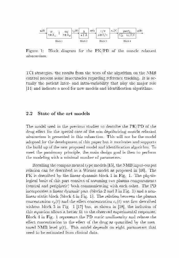
Block 1 Block 2 Block 3 Block 4

Figure 1: Block diagram for the PK/PD of the muscle relaxantatracurium.

TCI strategies, the results from the tests of the algorithm on the NMBcontrol present some inaccuracies regarding reference tracking. It is ac-tually the patient inter- and intra-variability that play the major role[14] and indicate a need for new models and identi�cation algorithms.

2.2 State of the art models

The model used in the previous studies to describe the PK/PD of thedrug e�ect for the special case of the non-depolarizing muscle relaxantatracurium is presented in this subsection. This will not be the modeladopted for the development of this paper but it motivates and supportsthe build up of the new proposed model and identi�cation algorithm. Tomeet the parsimony principle, the main design goal is then to performthe modeling with a minimal number of parameters.

Recalling the compartmental type models [15], the NMB input-outputrelation can be described as a Wiener model as proposed in [16]. ThePK is described by the linear dynamic block 1 in Fig. 1. The physio-logical basis of this part consists of assuming two plasma compartments(central and peripheric) both communicating with each other. The PDincorporates a linear dynamic part (blocks 2 and 3 in Fig. 1) and a non-linear static block (block 4 in Fig. 1). The relation between the plasmaconcentration cp(t) and the e�ect concentration ce(t) was �rst describedwithout block 3 in Fig. 1 [17] but, as shown in [18], the inclusion ofthis equation allows a better �t to the observed experimental responses.Block 4 in Fig. 1 represents the PD static nonlinearity and relates thee�ect concentration to the e�ect of the drug as quanti�ed by the mea-sured NMB level y(t). This model depends on eight parameters thatneed to be estimated from clinical data.

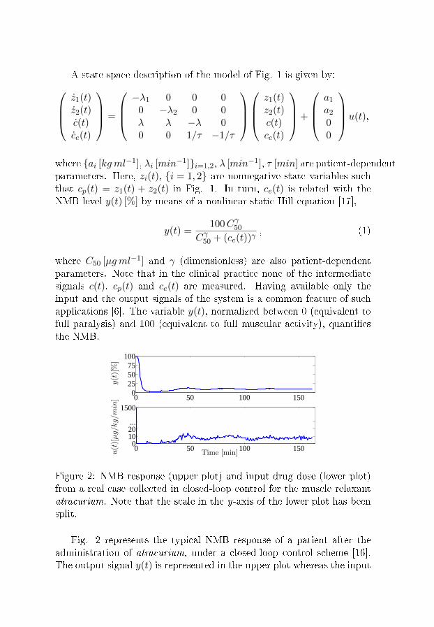
A state space description of the model of Fig. 1 is given by:z1(t)z2(t)c(t)ce(t)

=

−λ1 0 0 0

0 −λ2 0 0λ λ −λ 00 0 1/τ −1/τ

z1(t)z2(t)c(t)ce(t)

+

a1a200

u(t),

where {ai [kgml−1], λi [min−1]}i=1,2, λ [min−1], τ [min] are patient-dependentparameters. Here, zi(t), {i = 1, 2} are nonnegative state variables suchthat cp(t) = z1(t) + z2(t) in Fig. 1. In turn, ce(t) is related with theNMB level y(t) [%] by means of a nonlinear static Hill equation [17],

y(t) =100Cγ50

Cγ50 + (ce(t))γ, (1)

where C50 [µgml−1] and γ (dimensionless) are also patient-dependentparameters. Note that in the clinical practice none of the intermediatesignals c(t), cp(t) and ce(t) are measured. Having available only theinput and the output signals of the system is a common feature of suchapplications [6]. The variable y(t), normalized between 0 (equivalent tofull paralysis) and 100 (equivalent to full muscular activity), quanti�esthe NMB.

0 50 100 1500

255075

100

y(t)[%]

0 50 100 1500

1020...

1500

Time [min]u(t)[µg/k

g/m

in]

Figure 2: NMB response (upper plot) and input drug dose (lower plot)from a real case collected in closed-loop control for the muscle relaxantatracurium. Note that the scale in the y-axis of the lower plot has beensplit.

Fig. 2 represents the typical NMB response of a patient after theadministration of atracurium, under a closed-loop control scheme [16].The output signal y(t) is represented in the upper plot whereas the input

drug dose u(t) is shown in the lower plot. As can be seen in the lowerplot, at the beginning of the surgery, during the so-called induction phase(t ≤ 10min), a bolus of atracurium, typically uδ = 500 δ(t)µg kg−1

(in discrete-time corresponding to u(0) = uδ h with h = 1/3min−1) isadministered to the patient to enable a rapid drop of NMB level. Forcontrol purposes, during the period where the patient is under the e�ectof the bolus drug dose (t ≤ 30min for atracurium), the value of thereference is �xed at a low level, being gradually raised to the setpoint of10% [16]. The output signal y(t) represented in the upper plot of Fig. 2was then maintained around the reference pro�le by the administrationof the input drug dose u(t), calculated by a closed-loop control strategy[19].

Due to the characteristics of the true system present in this applica-tion, the available input signals vary less than desirable when the goalis to design reliable system identi�cation algorithms. Hence, �nding thebest model, in terms of parsimony, to explain the system with the partic-ular characteristics of poor excitation and limited datasets to work withmotivates the present study.

3 New model: minimal number of parameters

A new SISO Wiener model describing atracurium PK/PD is presentedin this section. One adaptive algorithm for simultaneous identi�cationof the linear dynamics and the static nonlinearity is then derived. Mo-dels are �rst constructed using a continuous-time Wiener model. Thismodel is then sampled with a zero-order hold strategy [20]. This en-ables the derivation of the EKF algorithm that estimates the under-lying continuous-time parameters, thereby exploiting the fact that thecontinuous-time parameters are of minimal number.

3.1 Linear block

For simulation purposes, and in order to cover a wide range of behaviors,a bank of realistic nonlinear dynamic models for atracurium PK/PD wasgenerated using the probabilistic distribution discussed in [18]. It thenconstitutes a simulated database where the exact parameterization of (1)and (1) is known for each simulated patient.

Fig. 3 shows, in solid line, the e�ect concentration response (outputfrom the linear dynamic part in the Wiener model) of model number25 in the simulated database after administration of a single atracurium

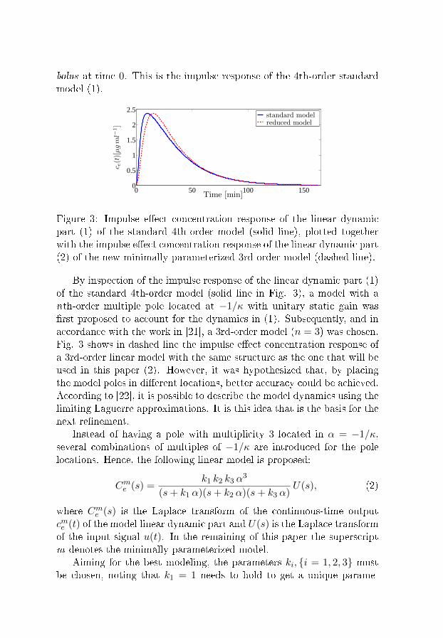
bolus at time 0. This is the impulse response of the 4th-order standardmodel (1).

0 50 100 1500

0.5

1

1.5

2

2.5

Time [min]

c e(t)[µgml−

1]

standard modelreduced model

Figure 3: Impulse e�ect concentration response of the linear dynamicpart (1) of the standard 4th-order model (solid line), plotted togetherwith the impulse e�ect concentration response of the linear dynamic part(2) of the new minimally parameterized 3rd-order model (dashed line).

By inspection of the impulse response of the linear dynamic part (1)of the standard 4th-order model (solid line in Fig. 3), a model with anth-order multiple pole located at −1/κ with unitary static gain was�rst proposed to account for the dynamics in (1). Subsequently, and inaccordance with the work in [21], a 3rd-order model (n = 3) was chosen.Fig. 3 shows in dashed line the impulse e�ect concentration response ofa 3rd-order linear model with the same structure as the one that will beused in this paper (2). However, it was hypothesized that, by placingthe model poles in di�erent locations, better accuracy could be achieved.According to [22], it is possible to describe the model dynamics using thelimiting Laguerre approximations. It is this idea that is the basis for thenext re�nement.

Instead of having a pole with multiplicity 3 located in α = −1/κ,several combinations of multiples of −1/κ are introduced for the polelocations. Hence, the following linear model is proposed:

Cme (s) =k1 k2 k3 α

3

(s+ k1 α)(s+ k2 α)(s+ k3 α)U(s), (2)

where Cme (s) is the Laplace transform of the continuous-time outputcme (t) of the model linear dynamic part and U(s) is the Laplace transformof the input signal u(t). In the remaining of this paper the superscriptm denotes the minimally parameterized model.

Aiming for the best modeling, the parameters ki, {i = 1, 2, 3} mustbe chosen, noting that k1 = 1 needs to hold to get a unique parame-

terization. A brute force search on the available real database was thenperformed in [21]. The combination k2 = 4 and k3 = 10 was the onethat proved to be optimal for the all cases in the database, meaningthat the normalized error was found to be minimum for those values.The constants k2 and k3 are then �xed to 4 and 10, respectively, in allsimulations that give rise to the results present in the remaining of thispaper.

3.2 Nonlinear block

The output from the nonlinear block was modeled with the Hill equation:

ym(t) =100Cγ50

Cγ50 + (cme (t))γ. (3)

Here θ = (α , γ) T is the parameter vector. The parameter α of thelinear dynamics (2) and the parameter γ of the nonlinearity (3) are hencejointly identi�ed.

Noting that the linear part contributes with a unit gain for the wholesystem, the di�erential static gain must be estimated by the parameterto be adapted in the nonlinear part [6]. At the same time, γ adapts theshape or static di�erential gain of (3). According to [9], in simulationstudies on the previously mentioned simulated database, the variabilityon C50 does not strongly a�ect the identi�cation results. Hence C50 waskept constant during this study.

3.3 Sampling

In order to implement the proposed model structure in the identi�cationalgorithm, the continuous-time representation (2) has to be sampled. Forthat purpose, the system (2) was represented in a state-space form asfollows, {

x(t) = A(α)x(t) +B(α)u(t)cme (t) = C(α)x(t)

, (4)

where u(t) ∈ R is the input (drug dose infusion), x(t) ∈ R3×1 is the con-tinuous model state-vector, cme (t) ∈ R is the output (e�ect concentrationof the drug), and C(α) ∈ R1×3, A(α) ∈ R3×3 and B(α) ∈ R3×1 arethe system matrices. Note that k′is are not shown explicitly in (4) sincethey are determined a priori in a single optimization step with respectto the available data, and �xed in the identi�cation simulations to be

performed afterwards. Because of this, the parameter α is the only oneto be adapted in order to cover the patients' dynamics variability in thelinear part.

The zero-order hold method [20] was applied using the sampling in-stant tk = kh. Usually, h is equal to 1/3min−1 due to the fact that,in the surgery environment, data from NMB is monitored and acquiredevery 20 sec = 1/3min−1. The discrete-time model then becomes{

x(kh+ h) = Φ(α)x(kh) + Γ(α)u(kh)cme (kh) = C(α)x(kh)

, (5)

whereΦ(α) = eA(α)h

Γ(α) =∫ h0 e

A(α)s dsB(α). (6)

Here, u(kh) ∈ R is the input (piecewise constant drug dose infusion),x(kh) ∈ R3×1 is the discrete model state-vector, cme (kh) ∈ R is theoutput (e�ect concentration of the drug), and Γ(α) ∈ R3×3 and B(α) ∈R3×1 are the sampled system matrices.

The sampling does not a�ect the nonlinear block, hence (3) can beused as it is. The model output is then given by:

ym(kh) =100Cγ50

Cγ50 + (cme (kh))γ. (7)

4 Recursive identi�cation algorithm:

Extended Kalman Filter

In order to enable the incorporation of a nonlinear identi�cation algo-rithm in an online platform for control of NMB, recursive identi�cationmethodologies need to be developed. This is e.g. a prerequisite whenadaptive control is introduced [23]. The Extended Kalman Filter (EKF)is then a natural choice since it is well suited for adaptive control struc-tures using e.g. Model Predictive Control (MPC). Moreover, dependingon its formulation, it also provides values for the state estimates in ev-ery iteration step, these being needed for MPC control. The idea of theEKF is to use the Kalman �lter [24] for a nonlinear problem. The EKF,in contrast to the Kalman �lter for linear systems, is not an optimal�lter. Nevertheless, it constitutes a powerful tool for recursively identi-fying the model parameters. In contrast to other recursive identi�cationtechniques it also has the advantage of independent tuning using the

covariance matrix of both the process and measurement noise, therebyenabling a tuning of the speed of convergence for each parameter sepa-rately. For EKF purposes, the general discrete nonlinear model is

x(t+ 1) = f(t, x(t), u(t)) + g(t, x(t)) v(t)y(t) = h(t, x(t)) + e(t)

,

where v(t) and e(t) are mutually independent Gaussian white noise se-quences with zero means and covariances R1(t) and R2(t), respectively.The EKF algorithm can then be summarized as follows [24]:

H(t) =∂h(t, x)

∂x

∣∣∣∣x=x(t|t−1)

K(t) = P (t|t− 1)HT (t)× [H(t)P (t|t− 1)HT (t) +R2(t)]−1

x(t|t) = x(t|t− 1) +K(t)[y(t)− h(t, x(t|t− 1))]

P (t|t) = P (t|t− 1)−K(t)H(t)P (t|t− 1)

x(t+ 1|t) = f(t, x(t|t), u(t))

F (t) =∂f(t, x)

∂x

∣∣∣∣x=x(t|t)

(8)

G(t) = g(t, x)∣∣x=x(t|t)

P (t+ 1|t) = F (t)P (t|t)F T (t) +G(t)R1(t)GT (t)

In the next subsection, the recursive identi�cation setting of the EKFis derived.

4.1 Model structural aspects

To enable the estimation of the model parameters with the EKF, a cou-pled identi�cation model must be de�ned. The model merges the sam-pled model (5) and a random walk model for the parameter estimates[11]:

x(kh) =

x1(kh)x2(kh)x3(kh)x4(kh)x5(kh)

=

x1(kh)x2(kh)x3(kh)α(kh)γ(kh)

. (9)

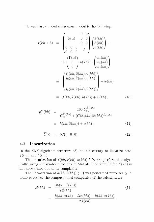
Hence, the extended state-space model is the following:

x(kh+ h) =

Φ(α)

0 00 00 0

0 0 00 0 0

I

x(kh)α(kh)γ(kh)

+

+

Γ(α)00

u(kh) +

wx(kh)wα(kh)wγ(kh)

≡

f1(kh, x(kh), u(kh))

f2(kh, x(kh), u(kh))...

f5(kh, x(kh), u(kh))

+ w(kh)

≡ f(kh, x(kh), u(kh)) + w(kh) , (10)

ym(kh) =100 C

x5(kh)50

Cx5(kh)50 + (C(x4(kh))x(kh))x5(kh)

≡ h(kh, x(kh)) + e(kh) , (11)

C(·) = (C(·) 0 0) . (12)

4.2 Linearization

In the EKF algorithm structure (8), it is necessary to linearize bothf(t, x) and h(t, x).

The linearization of f(kh, x(kh), u(kh)) (10) was performed analyt-ically, using the symbolic toolbox of Matlab. The formula for F (kh) isnot shown here due to its complexity.

The linearization of h(kh, x(kh)) (11) was performed numerically inorder to reduce the computational complexity of the calculations:

H(kh) =∂h(kh, x(kh))

∂x(kh)(13)

=h(kh, x(kh) + ∆x(kh))− h(kh, x(kh))

∆x(kh),

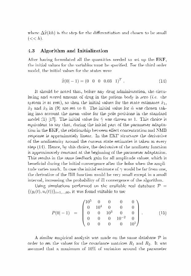
where ∆x(kh) is the step for the di�erentiation and chosen to be small(<< h).

4.3 Algorithm and Initialization

After having formulated all the quantities needed to set up the EKF,the initial values for the variables must be speci�ed. For the third-ordermodel, the initial values for the states were

x(0| − 1) = (0 0 0 0.03 1)T . (14)

It should be noted that, before any drug administration, the circu-lating and stored amount of drug in the patient body is zero (i.e. thesystem is at rest), so then the initial values for the state estimates x1,x2 and x3 in (9) are set to 0. The initial value for α was chosen tak-ing into account the mean value for the pole positions in the standardmodel (1) [17]. The initial value for γ was chosen as 1. This choice isequivalent to say that, during the initial part of the parameter adapta-tion in the EKF, the relationship between e�ect concentration and NMBresponse is approximately linear. In the EKF structure the derivativeof the nonlinearity around the current state estimates is taken at everystep (14). Hence, by this choice, the derivative of the nonlinear functionis approximately constant at the beginning of the parameter adaptation.This results in the same feedback gain for all amplitude values, which isbene�cial during the initial convergence after the bolus when the ampli-tude varies much. In case the initial estimate of γ would be far from one,the derivative of the Hill function would be very small except in a smallinterval, increasing the probability of ill convergence of the algorithm.

Using simulations performed on the available real database P ={(yi(t), ui(t))}i=1,...,60, it was found suitable to use

P (0| − 1) =

105 0 0 0 00 104 0 0 00 0 103 0 00 0 0 10−2 00 0 0 0 101

. (15)

A similar empirical analysis was made on the same database P inorder to set the values for the covariance matrices R1 and R2. It wasassumed that a maximum of 10% of variation around the parameter

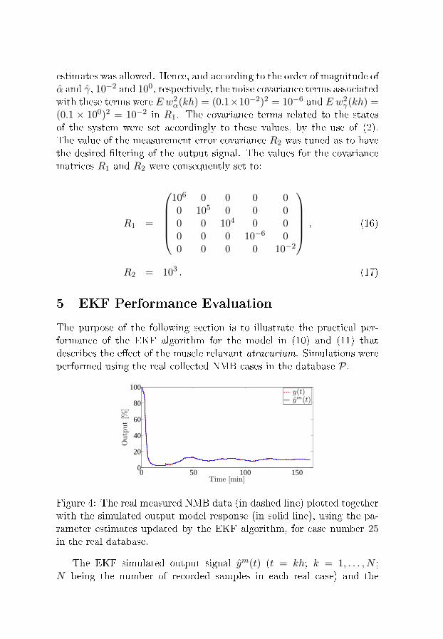
estimates was allowed. Hence, and according to the order of magnitude ofα and γ, 10−2 and 100, respectively, the noise covariance terms associatedwith these terms were E w2

α(kh) = (0.1×10−2)2 = 10−6 and E w2γ(kh) =

(0.1 × 100)2 = 10−2 in R1. The covariance terms related to the statesof the system were set accordingly to these values, by the use of (2).The value of the measurement error covariance R2 was tuned as to havethe desired �ltering of the output signal. The values for the covariancematrices R1 and R2 were consequently set to:

R1 =

106 0 0 0 00 105 0 0 00 0 104 0 00 0 0 10−6 00 0 0 0 10−2

, (16)

R2 = 103 . (17)

5 EKF Performance Evaluation

The purpose of the following section is to illustrate the practical per-formance of the EKF algorithm for the model in (10) and (11) thatdescribes the e�ect of the muscle relaxant atracurium. Simulations wereperformed using the real collected NMB cases in the database P.

0 50 100 1500

20

40

60

80

100

Time [min]

Output[%

]

y(t)ym(t)

Figure 4: The real measured NMB data (in dashed line) plotted togetherwith the simulated output model response (in solid line), using the pa-rameter estimates updated by the EKF algorithm, for case number 25in the real database.

The EKF simulated output signal ym(t) (t = kh; k = 1, . . . , N ;N being the number of recorded samples in each real case) and the

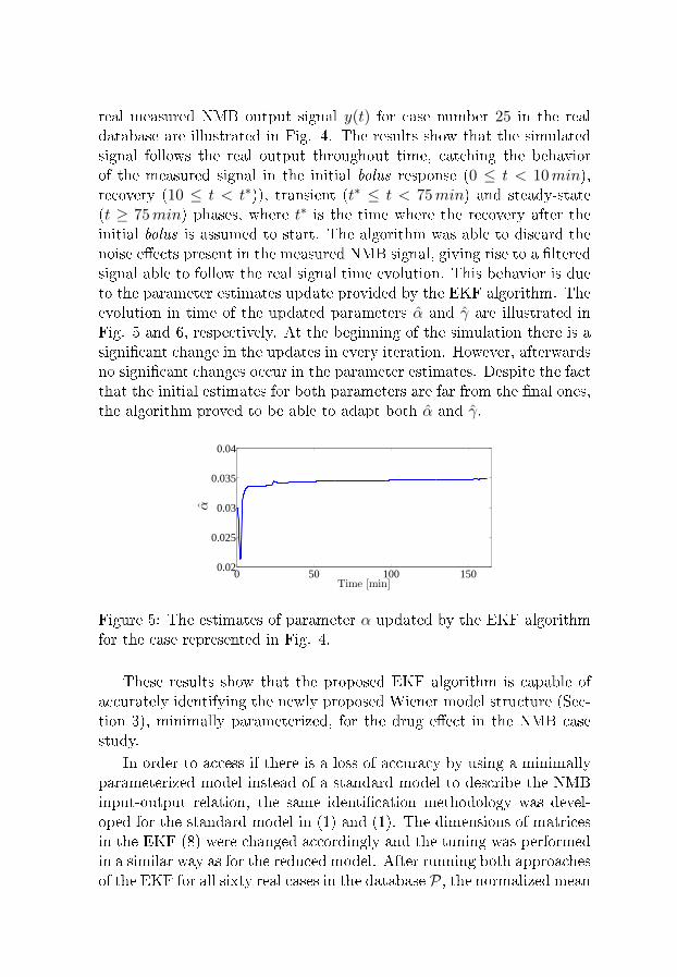
real measured NMB output signal y(t) for case number 25 in the realdatabase are illustrated in Fig. 4. The results show that the simulatedsignal follows the real output throughout time, catching the behaviorof the measured signal in the initial bolus response (0 ≤ t < 10min),recovery (10 ≤ t < t∗)), transient (t∗ ≤ t < 75min) and steady-state(t ≥ 75min) phases, where t∗ is the time where the recovery after theinitial bolus is assumed to start. The algorithm was able to discard thenoise e�ects present in the measured NMB signal, giving rise to a �lteredsignal able to follow the real signal time evolution. This behavior is dueto the parameter estimates update provided by the EKF algorithm. Theevolution in time of the updated parameters α and γ are illustrated inFig. 5 and 6, respectively. At the beginning of the simulation there is asigni�cant change in the updates in every iteration. However, afterwardsno signi�cant changes occur in the parameter estimates. Despite the factthat the initial estimates for both parameters are far from the �nal ones,the algorithm proved to be able to adapt both α and γ.

0 50 100 1500.02

0.025

0.03

0.035

0.04

Time [min]

α

Figure 5: The estimates of parameter α updated by the EKF algorithmfor the case represented in Fig. 4.

These results show that the proposed EKF algorithm is capable ofaccurately identifying the newly proposed Wiener model structure (Sec-tion 3), minimally parameterized, for the drug e�ect in the NMB casestudy.

In order to access if there is a loss of accuracy by using a minimallyparameterized model instead of a standard model to describe the NMBinput-output relation, the same identi�cation methodology was devel-oped for the standard model in (1) and (1). The dimensions of matricesin the EKF (8) were changed accordingly and the tuning was performedin a similar way as for the reduced model. After running both approachesof the EKF for all sixty real cases in the database P, the normalized mean

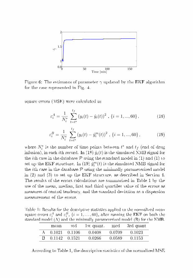
0 50 100 1500.8

1

1.5

2

Time [min]

γ

Figure 6: The estimates of parameter γ updated by the EKF algorithmfor the case represented in Fig. 4.

square errors (MSE) were calculated as

εAi =1

N∗i

tf∑t=t∗

(yi(t)− yi(t))2 , {i = 1, ..., 60} , (18)

εBi =1

N∗i

tf∑t=t∗

(yi(t)− ymi (t))2 , {i = 1, ..., 60} , (19)

where N∗i is the number of time points between t∗ and tf (end of druginfusion), in each ith record. In (18) yi(t) is the simulated NMB signal forthe ith case in the database P using the standard model in (1) and (1) toset up the EKF structure. In (19) ymi (t) is the simulated NMB signal forthe ith case in the database P using the minimally parameterized modelin (2) and (3) to set up the EKF structure, as described in Section 4.The results of the errors calculations are summarized in Table 1 by theuse of the mean, median, �rst and third quartiles value of the errors asmeasures of central tendency, and the standard deviation as a dispersionmeasurement of the errors.

Table 1: Results for the descriptive statistics applied to the normalized meansquare errors εAi and εBi , {i = 1, . . . , 60}, after running the EKF on both thestandard model (A) and the minimally parameterized model (B) for the NMB.

mean std 1st quant. med 3rd quant

A 0.1021 0.1106 0.0408 0.0709 0.1023

B 0.1142 0.1521 0.0266 0.0589 0.1153

According to Table 1, the descriptive statistics of the normalized MSE

obtained after running the EKF on both the standard and minimallyparameterized models gives similar results. According to this statistics,the EKF based on the new minimally parameterized model gives rise toidenti�cation results as accurate as the ones obtained when the EKF isderived for the standard model.

As a natural consequence of these results, it was hypothesized that ifthe identi�cation performances are almost the same, one of the poles andthe zero in the standard model should cancel out or, at least, have valuesclose to each other. Hence, the values for the zero and poles of the lineartransfer function in the standard model (blocks 1, 2 and 3 in Fig. 1) werecalculated using the average value of each parameter estimate obtainedafter the initial bolus recovery. The pole-zero map for case number 25in the real database is shown in the middle plot of Fig. 7. The pole andthe zero closest to each other for each ith case in P (the ones that layinside the boxes in Fig. 7) correspond to:

pi = − 1

N∗i

tf∑t=t∗

λ(t) , (20)

zi = − 1

N∗i

tf∑t=t∗

a1(t) λ2(t) + a2(t) λ1(t)

a1(t) + a2(t), (21)

respectively.The distance ∆i = |pi − zi| between pole pi (20) and zero zi (21)

for all sixty cases in the database P was calculated. The position of thepoles and zero for the cases with the minimum and the maximum valueof ∆ are shown in the bottom and upper plot of Fig. 7, respectively.

The results present in Fig. 7 show that there is actually one zero andone pole close to each other when the standard model (1) and (1) is usedto describe the NMB input-output relation in the real records. This factis a further indication that the minimally parameterized model structureretains the main characteristics of the system, with the advantage ofusing few number of independent parameters.

6 Conclusion

This paper presented a new strategy of modeling and identi�cation ofphysiological nonlinear Wiener systems. The example of NeuroMuscularBlockade (NMB) was used. The newly developed minimally parameteri-zed Wiener model for the e�ect of the muscle relaxant atracurium proved

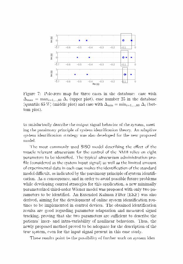
−0.7 −0.6 −0.5 −0.4 −0.3 −0.2 −0.1 0−1

0

1

Im (

s)

−0.7 −0.6 −0.5 −0.4 −0.3 −0.2 −0.1 0−1

0

1Im

(s)

−0.7 −0.6 −0.5 −0.4 −0.3 −0.2 −0.1 0−1

0

1

Re (s)

Im (

s)

Figure 7: Pole-zero map for three cases in the database: case with∆max = maxi=1,...,60 ∆i (upper plot), case number 25 in the database(quantile 65 %) (middle plot) and case with ∆min = mini=1,...,60 ∆i (bot-tom plot).

to satisfactorily describe the output signal behavior of the system, meet-ing the parsimony principle of system identi�cation theory. An adaptivesystem identi�cation strategy was also developed for the new proposedmodel.

The most commonly used SISO model describing the e�ect of themuscle relaxant atracurium for the control of the NMB relies on eightparameters to be identi�ed. The typical atracurium administration pro-�le (considered as the system input signal) as well as the limited amountof experimental data in each case makes the identi�cation of the standardmodel di�cult, as indicated by the parsimony principle of system identi�-cation. As a consequence, and in order to avoid possible future problemswhile developing control strategies for this application, a new minimallyparameterized third-order Wiener model was proposed with only two pa-rameters to be identi�ed. An Extended Kalman Filter (EKF) was alsoderived, aiming for the development of online system identi�cation rou-tines to be implemented in control devices. The obtained identi�cationresults are good regarding parameter adaptation and measured signaltracking, proving that the two parameters are su�cient to describe thepatients' inter- and intra-variability of nonlinear behaviors. Thus, thenewly proposed method proved to be adequate for the description of thetrue system, even for the input signal present in this case study.

These results point to the possibility of further work on system iden-

ti�cation techniques for minimally parameterized models in anesthesia,namely the adaptation of these algorithms to the Depth of Anesthesia(DoA) case, using the Bispectral Index (BIS) signal. Further studies oninitialization algorithms as well as on the convergence properties of thedeveloped methods are also recommended to ensure a safe incorporationof such system identi�cation strategies in anesthesia integrated controlplatforms.

Acknowledgments

The authors would like to thank Fundação para a Ciência e Tecnolo-gia who partially funded the research present on this paper throughthe project IDeA (ref. PTDC/EEA-ACR/69288/2006) and the projectGaleno (ref. PTDC/SAU-BEB/103667/2008), and the Bernt Järmarksfoundation for the scienti�c research stipend. The research leading tothese results has also received funding from the European ResearchCouncil under the European Community's Seventh Framework Programme(FP7/2007-2013) / ERC grant agreement n. 247035.

References

[1] G. Widman, T. Schreiber, B. Redhberg, A. Hoeft, and C. E. Elger,�Quanti�cation of depth of anesthesia by nonlinear time series anal-ysis of brain electrical activity,� Physical Review, vol. 62, no. 4, pp.4898�4903, 2000.

[2] M. M. R. F. Struys, E. W. Jensen, W. Smith, N. T. Smith, I. Rampil,F. J. E. Dumortier, C. Mestach, and E. P. Mortier, �Performance ofthe ARX-derived auditory evoked potential index as an indicator ofanesthetic depth: A comparison with Bispectral Index and hemo-dynamic measures during propofol administration,� Anesthesiology,vol. 96, pp. 803�816, 2002.

[3] J. Bruhn, H. Röpcke, and A. Hoeft, �Approximate entropy as anelectroencephalographic measure of anesthetic drug e�ect duringdes�urane anesthesia,� Anesthesiology, vol. 92, pp. 715�726, 2000.

[4] P. S. Glass, M. Bloom, L. Kearse, C. Rosow, P. Sebel, and P. Man-berg, �Bispectral analysis measures sedation and memory e�ects of

propofol, midazolam, iso�urane, and alfentanil in healthy volun-teers,� Anesthesiology, vol. 86, pp. 836�847, 1997.

[5] S. Schraag, �Theoretical basis of target controlled anaesthesia: his-tory, concept and clinical perspectives,� Best Practice and Research

Clinical Anaesthesiology, vol. 15, no. 1, pp. 1�17, 2001.

[6] T. Wigren, �Recursive prediction error identi�cation method usingthe nonlinear Wiener model,� Automatica, vol. 29, no. 4, pp. 1011�1025, 1993.

[7] H.-H. Lin, C. L. Beck, and M. J. Bloom, �On the use of multi-variable piecewise-linear models for predicting human response toanesthesia,� IEEE Trans. Biomed. Eng., pp. 1876�1887, Nov. 2004.

[8] H. Alonso, T. Mendonça, J. M. Lemos, and T. Wigren, �A sim-ple model for the identi�cation of drug e�ects,� in Proc. IEEE In-

ternational symposium on Intelligent Signal Processing (WISP'09),Budapest, Hungary, 2009, pp. 269�273.

[9] H. Alonso, T. Mendonça, and P. Rocha, �A hybrid method for para-meter estimation and its application to biomedical systems,� Com-

puter Methods and Programs in Biomedicine, vol. 89, pp. 112�122,2008.

[10] T. Wigren, MATLAB software for Recursive Identi�cation of

Wiener Systems - Revision 2. Uppsala, Sweden: Uppsala Uni-versity, 2007.

[11] T. Söderström and P. Stoica, System Identi�cation. Hemel Hemp-stead, UK: Prentice-Hall, 1989.

[12] Diprifusor: Target Controlled Infusion (TCI) in anaesthetic prac-

tice, AstraZeneca, Alderley House, Alderley Park, Maccles�eld,Cheshire, UK, 1999.

[13] M. M. Silva, H. Alonso, J. M. Lemos, and T. Mendonça, �An adap-tive approach to target controlled infusion,� in Proc. European Con-

trol Conference (ECC'09), Budapest, Hungary, 2009, pp. 418�423.

[14] T. Mendonça, J. M. Lemos, H. Magalhães, P. Rocha, and S. Esteves,�Drug delivery for neuromuscular blockade with Supervised Multi-model Adaptive Control,� IEEE Trans. Control Syst. Technol., pp.1237�1244, Nov. 2009.

[15] K. Godfrey, Compartmental models and their application. AcademicPress, 1983.

[16] T. Mendonça and P. Lago, �PID control strategies for the automaticcontrol of neuromuscular blockade,� Control Engineering Practice,vol. 6, no. 10, pp. 1225�1231, 1998.

[17] B. Weatherley, S. Williams, and E. Neill, �Pharmacokinetics, phar-macodynamics and dose-response relationships of atracurium ad-ministered i. v.� Br. J. Anaesth., vol. 55, pp. 39s�45s, 1983.

[18] P. Lago, T. Mendonça, and L. Gonçalves, �On-line autocalibrationof a PID controller of neuromuscular blockade,� in Proc. of the 1998

IEEE International Conference on Control Applications, Trieste,Italy, 1998, pp. 363�367.

[19] M. M. Silva, T. Mendonça, and S. Esteves, �Personalized neuromus-cular blockade through control: clinical and technical evaluation,�in Proc. of the 30th Annual International Conference of the IEEE

Engineering in Medicine and Biology Society, Vancouver, Canada,2008, pp. 5826�5829.

[20] K. J. Åström and B. Wittenmark, Computer-Controlled Systems.Englewood Cli�s, NJ: Prentice Hall, 1984.

[21] M. M. Silva, T. Wigren, and T. Mendonça, �Nonlinearidenti�cation of a minimal neuromuscular blockade modelin anaesthesia,� Dept. Information Technology, Uppsala Uni-versity, Uppsala, Sweden, Tech. Rep. 2009-023, Available:http://www.it.uu.se/research/publications/reports/, Sept. 2009.

[22] B. Wahlberg, �System identi�cation using Laguerre models,� IEEETrans. Autom. Control, pp. 551�562, Jan. 1991.

[23] K. J. Åström and B. Wittenmark, Adaptive Control. Reading, MA:Addison-Wesley, 1989.

[24] T. Söderström, Discrete-time Stochastic Systems. London, UK:Springer-Verlag, 2002.

Paper II

Online nonlinear identi�cation of the

e�ect of drugs in anaesthesia using a

minimal parameterization and BIS

measurements

Margarida M. Silva, Teresa Mendonça and Torbjörn Wigren

Abstract

This paper addresses the problem of modeling and identi�ca-tion of the Depth of Anaesthesia (DoA). It presents a new MISOWiener model for the pharmacokinetics and pharmacodynamicsof propofol and remifentanil, when jointly administered to pa-tients undergoing surgery. The models most commonly used todescribe the e�ect of drugs in the human body are overparameter-ized Wiener models. In particular, in an anaesthesia environment,the high number of patient-dependent parameters coupled with theinsu�cient excitatory pattern of the input signals (drug dose pro-�les) and the presence of noise make robust identi�cation strategiesdi�cult to �nd. In fact, in such clinical application the user cannotfreely choose the input signals to enable accurate parameter iden-ti�cation. A new MISO Wiener model with only four parametersis hence proposed to model the e�ect of the joint administrationof the hypnotic propofol and the analgesic remifentanil. An Ex-tended Kalman Filter (EKF) algorithm was used to perform thenonlinear online identi�cation of the system parameters. The re-sults show that both the new model and the identi�cation strategyoutperform the currently used tools to infer individual patient res-ponse. The proposed DoA identi�cation scheme was evaluated ina real patient database, where the DoA is quanti�ed by the Bis-pectral Index Scale (BIS) measurements. The results obtained sofar indicate that the developed approach will be a powerful tool formodeling and identi�cation of anaesthetic drug dynamics duringsurgical procedures.

1 Introduction

The starting point for the mathematical modeling of physiological sys-tems is usually the background knowledge of the chemical or physi-cal laws present in such systems. In this sense, the deduced modelvariables are meaningful and can easily be interpreted as masses, vol-umes or even temperatures. The human response to the administrationof drugs in anaesthesia is a good example of this. In what concernsdepth of anaesthesia (DoA), the response for the administration of hyp-notics and analgesics is commonly modeled as an high order pharmacoki-netic/pharmacodynamic (PK/PD) Wiener model [1]. Here the parame-ters to be identi�ed are compartment volumes, micro-constant rates formass transfers between compartments and drug clearances in the humanbody.

System identi�cation theory states that the identi�ed model is a com-promise between the richness of the data and the identi�ability of theparameters [2]. The application of system identi�cation strategies toidentify each patient response to drug administration in anaesthesia isa particularly complex issue. This is because a common feature of suchsystems is the poor excitation, meaning that the input signals (admin-istered drug doses) are not rich enough in frequency and amplitude toexcite all modes of the system [3], as it is usually modeled. This is sosince the data is obtained from the surgery room, where patient safety isthe prime concern. The tradeo� between complexity and identi�abilityis therefore addressed with minimal modeling in the present paper.

The e�ect of drugs in the human body can often be modeled bya linear mixing dynamics, in cascade with a static nonlinear functionthat describes the e�ect of the drug. As a consequence of this Wienerstructure (a linear block in series with a static nonlinearity [4]), theprediction of human response to drugs cannot be accurately performedby linear models [5, 6]. Moreover, and in order to address the problemof having to deal with a model with many parameters, [7] presents asimpli�cation of the model structure. In [7] it is also pointed out thatto obtain a good modeling of the response, a good estimation of the PKmodel is needed. This fact gives rise to the problem of selecting the beststructure to model the real cases. This idea was further developed in [8],where excellent results were obtained by nonlinear recursive identi�cationof the neuromuscular blockade level using a two parameter model.

The contribution of this paper is to present a new method for non-linear identi�cation of the e�ect of drugs in anaesthesia, by the use of

a new minimally parameterized Multiple-Input-Single-Output (MISO)Wiener model. As expected, this approach leads to a model whose pa-rameters have a reduced physiological meaning. However, even from theclinical point of view, this is not a crucial issue since improved resultsare achieved in what concerns parameter adaptation and output signaltracking. Furthermore, continuous time parameters are estimated, a factthat facilitates physiological interpretation.

The input signals consist of the dosage of propofol and remifen-tanil. The human e�ect output signal used in the paper is the clinically-validated electroencephalogram-derived Bispectral Index Scale (BIS) [9].It can be noted that the BIS is at the focal point of anaesthesia researchtoday. Ranging from 100% (completely �awake� clinical state) to 0%(isoelectric EEG) the BIS is widely used as an indicator of the DoA. In ageneral surgery environment, the BIS should be kept between 40% and60% to enable a faster emergence from anaesthesia [10] and a lower ad-ministered drug dosage [11]. The combined administration of hypnoticsand analgesics for induction and maintenance of DoA is a common prac-tice. The hypnotic is targeted to the loss of consciousness and preventsawareness, while the analgesic is given to supress pain. Indeed, the clin-ical advantage of this combined procedure is the synergistic increase inthe expected e�ects of both drugs based on the nonlinear concentration-e�ect relationships of the individual agents [12]. This evidence is modeledby a nonlinear interaction function between the two drugs.

The present paper is structured as follows. Section 2 describes thestate of the art of DoA modeling, while Section 3 presents both thelinear and nonlinear parts of the new minimally parameterized modelfor the BIS response. In Section 4 the algorithm is derived, followed bythe presentation of results when applied to patient data in Section 5.Conclusions follow in Section 6.

2 DoA: State of the art models

The most commonly used models in the literature to describe the PK andPD of the propofol (hypnotic) and remifentanil (analgesic) e�ects in thehuman body are described in this section. It should be stressed that thesemodels will not be the ones used for the development of the identi�cationmethodologies of this study. These models are discussed here to pointout the need for the development of new minimally parameterized modelsto match the parsimony principle of system identi�cation [2].

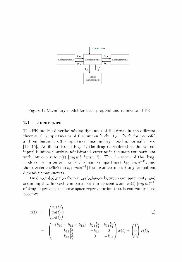
Compartment 2 Compartment 1 Compartment 3

Effect

Compartment

Figure 1: Mamillary model for both propofol and remifentanil PK

2.1 Linear part

The PK models describe mixing dynamics of the drugs in the di�erenttheoretical compartments of the human body [13]. Both for propofoland remifentanil, a 3-compartment mammilary model is normally used[14, 15]. As illustrated in Fig. 1, the drug (considered as the systeminput) is intravenously administrated, entering in the main compartmentwith infusion rate r(t) [mgml−1min−1]. The clearance of the drug,modeled by an outer �ow of the main compartment k10 [min−1], andthe transfer coe�cients kij [min−1] from compartment i to j are patientdependent parameters.

By direct deduction from mass balances between compartments, andassuming that for each compartment i, a concentration xi(t) [mgml−1]of drug is present, the state space representation that is commonly usedbecomes

x(t) =

x1(t)x2(t)x3(t)

(1)

=

−(k10 + k12 + k13) k21V2V1

k31V3V1

k12V1V2

−k21 0

k13V1V3

0 −k31

x(t) +

100

r(t),

where Vi [ml] represents the volume of compartment i.The PD nonlinearity relates the drug concentration with the e�ect,

DoA, and has a �rst linear dynamic part approximated by a �rst orderdi�erential equation [16]

xe(t) = ke0(x1(t)− xe(t)) , (2)

where ke0 is the inverse of the equilibrium time between the central com-partment (compartment 1 in Fig. 1) and the e�ect compartment, andxe(t) [mgml−1] is the e�ect compartment concentration (which cannotbe measured).

In clinical practice, population models are applied to infer the res-ponse of each patient to a certain drug administration pro�le. For propo-fol, the parameters from Marsh [17] or from Schnider [18] are usuallyused, whereas for remifentanil, the parameters from Minto [15] are com-monly applied.

2.2 Nonlinear interaction

This section describes the widely accepted nonlinear model for the in-teraction between propofol and remifentanil [19]. It relates the e�ectconcentration of both drugs with the electroencephalographic parametervalues e.g. BIS. Both e�ect concentrations xprope (t) and xremie (t) are �rstnormalized with respect to their concentration at half the maximal e�ect(ECprop50 and ECremi50 , respectively), i.e.

Uprop(t) = xprope (t)ECprop

50, Uremi(t) = xremi

e (t)

ECremi50

. (3)

As mentioned before, since the interaction of propofol and remifen-tanil is not purely additive, the potency of the drug mixture is modeledas follows

φ =Uprop(t)

Uprop(t) + Uremi(t), (4)

where, by de�nition, φ ranges from 0 (remifentanil only) and 1 (propofolonly). The nonlinear concentration-response relationship for any ratioof the two drugs can then be described by a generalized Hill equation as

y(t) = y0

1−

(Uprop(t)+Uremi(t)

U50(φ)

)γ1 +

(Uprop(t)+Uremi(t)

U50(φ)

)γ , (5)

where y0 is the e�ect at zero concentration, γ controls the steepness ofthe nonlinear concentration-response relation, and U50(φ) is the numberof units associated with 50% of the maximum e�ect of both drugs atratio φ. In [19] a quadratic polynomial was proposed for the expressionof U50(φ) :

U50(φ) = 1− βφ+ βφ2 . (6)

In common clinical practice, the parameters γ, β, ECprop50 and ECremi50

and the linear parameters kij and ke0 of (1) and (2) are usually guessedbased on population model distributions and on the clinicians' expertise.The result is a model depending on many continuous time parameters.

3 Minimally parameterized model

A new MISO Wiener model with a minimal number of parameters de-scribing the joint e�ect of propofol and remifentanil in the human bodyis presented in this section. Models are �rst built using a continuous-time description and then sampled with a zero-order hold strategy. Thismakes it possible to derive algorithms that estimate the underlying con-tinuous time parameters, exploiting the intrinsic feature of having a min-imal number of parameters.

3.1 Linear block

By inspection of the model structure, the plasmatic concentration (incompartment 1 of Fig. 1) and the e�ect concentration coming frompopulation studies for both propofol [18] and remifentanil [15], a third-order continuous time model is proposed for the linear dynamics of eachdrug. It can be noted that this approach was also very successful in [8].

Propofol linear dynamics is hence modeled by

Xprope (s, α) =

k1 k2 k3 α3

(s+ k1 α) (s+ k2 α) (s+ k3 α)Rprop(s), (7)

where Xprope (s, α) is the Laplace transform of the output from the model

linear dynamic part for propofol xprope (t, α) and Rprop(s) is the Laplacetransform of the input signal rprop(t). The pole location α is selected asthe parameter to be identi�ed.

Remifentanil linear dynamics is similarly modeled by

Xremie (s, η) =

l1 l2 l3 η3

(s+ l1 η) (s+ l2 η) (s+ l3 η)Rremi(s), (8)

where Xremie (s, η) is the Laplace transform of the output from the model

for remifentanil xremie (t, η) and Rremi(s) is the Laplace transform of theinput signal rremi(t). The pole location η is selected as the parameterto be identi�ed.

3.2 Nonlinear block

Using the model in (5) as starting point, a new formulation for thenonlinearity is now proposed. According to (6),

Uprop(t, α) + Uremi(t, η)

U50(φ)=Uprop(t, α) + Uremi(t, η)

1− βφ+ βφ2. (9)

Hence, to motivate the new model, consider |r| = |βφ − βφ2| to beless than 1 and exploit the Taylor series expansion

1

1− r= 1 + r + r2 + r3 + . . . (10)

Then, neglecting the high-order terms, and substituting φ accordingto (4), it follows

Uprop(t, α) + Uremi(t, η)

U50(φ)(11)

≈(Uprop(t, α) + Uremi(t, η)

)(1 + β

Uprop(t,α)

Uprop(t,α)+Uremi(t,η)

)= Uremi(t, η) + (1 + β) Uprop(t, α)

= Uremi(t, η) +mUprop(t, α).

Here m = 1 + β is selected as one of the parameters to be identi�ed.Furthermore, following (3),

Uprop(t, α) = xprope (t,α)ECprop

50, Uremi(t, η) = xremi

e (t,η)

ECremi50

. (12)

Hence, (5) is substituted by the new formulation:

y(t) =y0

1 +(Uremi(t, η) +mUprop(t, α)

)γ . (13)

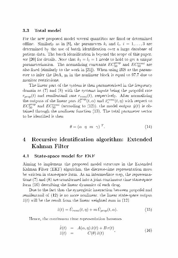
3.3 Total model

For the new proposed model several quantities are �xed or determinedo�ine. Similarly as in [8], the parameters ki and li, i = 1, . . . , 3 aredetermined by the use of batch identi�cation over a large database ofpatient data. The batch identi�cation is beyond the scope of this paper,see [20] for details. Note that k1 = l1 = 1 needs to hold to get a uniqueparameterization. The normalizing constants ECprop50 and ECremi50 arealso �xed (similarly to the work in [21]). When using BIS as the param-eter to infer the DoA, y0 in the nonlinear block is equal to 97.7 due tomonitor restrictions.

The linear part of the system is then parameterized in the frequencydomain as (7) and (8) with the systems inputs being the propofol raterprop(t) and remifentanil rate rremi(t), respectively. After normalizingthe outputs of the linear part xprope (t, α) and xremie (t, η) with respect toECprop50 and ECremi50 (according to (12)), the model output y(t) is ob-tained through the nonlinear function (13). The total parameter vectorto be identi�ed is then

θ = (α η m γ) T . (14)

4 Recursive identi�cation algorithm: Extended

Kalman Filter

4.1 State-space model for EKF

Aiming to implement the proposed model structure in the ExtendedKalman Filter (EKF) algorithm, the discrete-time representation mustbe written in state-space form. As an intermediate step, the representa-tions (7) and (8) are transformed into a joint continuous time state-spaceform (16) describing the linear dynamics of each drug.

Due to the fact that the synergistic interaction between propofol andremifentanil of (12) is no more nonlinear, the linear state-space outputz(t) will be the result from the linear weighted sum in (12)

z(t) = Uremi(t, η) +mUprop(t, α). (15)

Hence, the continuous-time representation becomes

˙x(t) = A(α, η) x(t) +B r(t)z(t) = C(θ) x(t)

, (16)

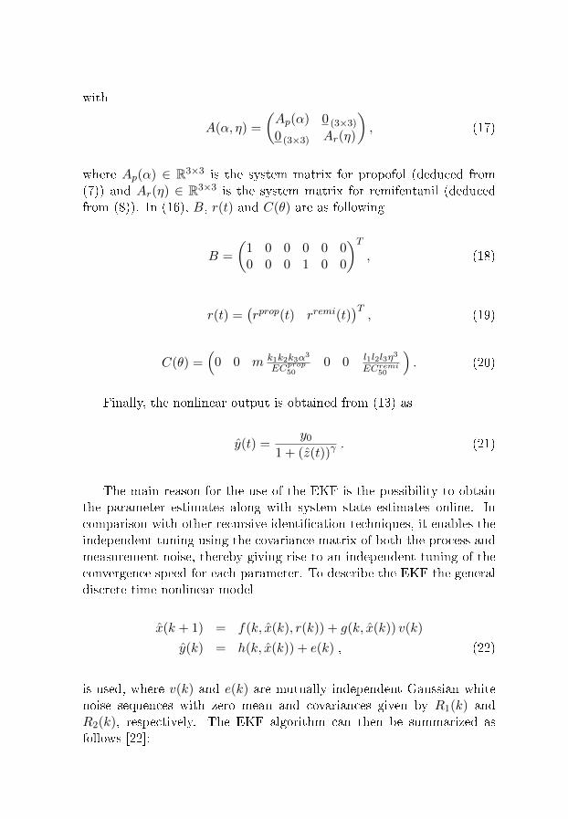
with

A(α, η) =

(Ap(α) 0 (3×3)

0 (3×3) Ar(η)

), (17)

where Ap(α) ∈ R3×3 is the system matrix for propofol (deduced from(7)) and Ar(η) ∈ R3×3 is the system matrix for remifentanil (deducedfrom (8)). In (16), B, r(t) and C(θ) are as following

B =

(1 0 0 0 0 00 0 0 1 0 0

)T, (18)

r(t) =(rprop(t) rremi(t)

)T, (19)

C(θ) =(

0 0 m k1k2k3α3

ECprop50

0 0 l1l2l3η3

ECremi50

). (20)

Finally, the nonlinear output is obtained from (13) as

y(t) =y0

1 + (z(t))γ. (21)

The main reason for the use of the EKF is the possibility to obtainthe parameter estimates along with system state estimates online. Incomparison with other recursive identi�cation techniques, it enables theindependent tuning using the covariance matrix of both the process andmeasurement noise, thereby giving rise to an independent tuning of theconvergence speed for each parameter. To describe the EKF the generaldiscrete time nonlinear model

x(k + 1) = f(k, x(k), r(k)) + g(k, x(k)) v(k)

y(k) = h(k, x(k)) + e(k) , (22)

is used, where v(k) and e(k) are mutually independent Gaussian whitenoise sequences with zero mean and covariances given by R1(k) andR2(k), respectively. The EKF algorithm can then be summarized asfollows [22]:

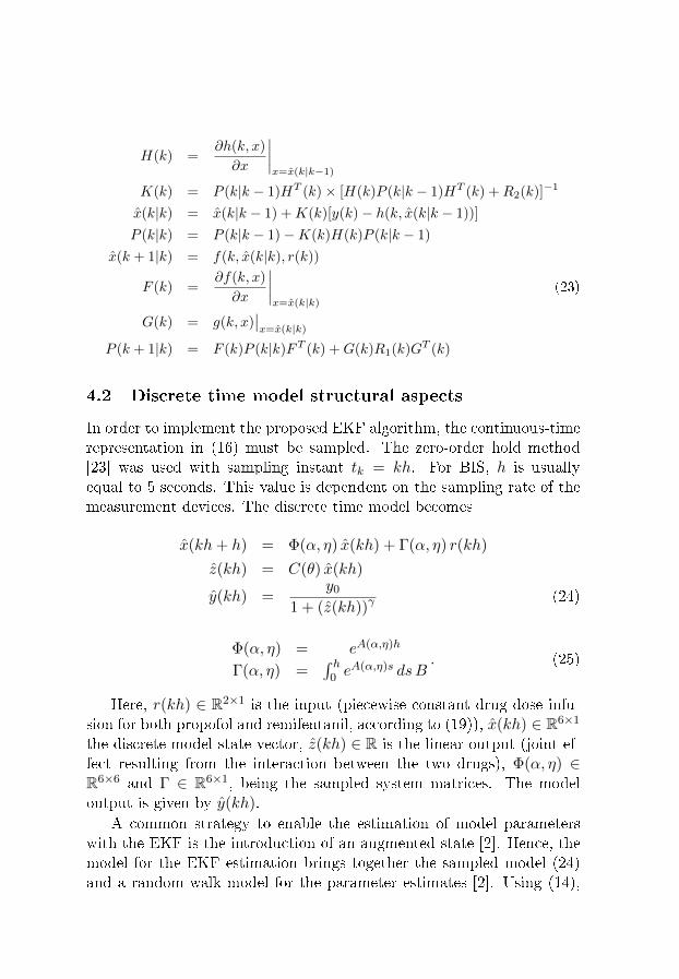
H(k) =∂h(k, x)

∂x

∣∣∣∣x=x(k|k−1)

K(k) = P (k|k − 1)HT (k)× [H(k)P (k|k − 1)HT (k) +R2(k)]−1

x(k|k) = x(k|k − 1) +K(k)[y(k)− h(k, x(k|k − 1))]

P (k|k) = P (k|k − 1)−K(k)H(k)P (k|k − 1)

x(k + 1|k) = f(k, x(k|k), r(k))

F (k) =∂f(k, x)

∂x

∣∣∣∣x=x(k|k)

(23)

G(k) = g(k, x)∣∣x=x(k|k)

P (k + 1|k) = F (k)P (k|k)FT (k) +G(k)R1(k)GT (k)

4.2 Discrete time model structural aspects

In order to implement the proposed EKF algorithm, the continuous-timerepresentation in (16) must be sampled. The zero-order hold method[23] was used with sampling instant tk = kh. For BIS, h is usuallyequal to 5 seconds. This value is dependent on the sampling rate of themeasurement devices. The discrete time model becomes

x(kh+ h) = Φ(α, η) x(kh) + Γ(α, η) r(kh)

z(kh) = C(θ) x(kh)

y(kh) =y0

1 + (z(kh))γ(24)

Φ(α, η) = eA(α,η)h

Γ(α, η) =∫ h0 e

A(α,η)s dsB. (25)

Here, r(kh) ∈ R2×1 is the input (piecewise constant drug dose infu-sion for both propofol and remifentanil, according to (19)), x(kh) ∈ R6×1

the discrete model state-vector, z(kh) ∈ R is the linear output (joint ef-fect resulting from the interaction between the two drugs), Φ(α, η) ∈R6×6 and Γ ∈ R6×1, being the sampled system matrices. The modeloutput is given by y(kh).

A common strategy to enable the estimation of model parameterswith the EKF is the introduction of an augmented state [2]. Hence, themodel for the EKF estimation brings together the sampled model (24)and a random walk model for the parameter estimates [2]. Using (14),

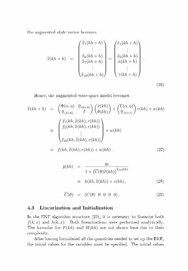
the augmented state vector becomes

x(kh+ h) =

x1(kh+ h)...

x6(kh+ h)

x7(kh+ h)...

x10(kh+ h)

=

x1(kh+ h)...

x6(kh+ h)α(kh+ h)

...γ(kh+ h)

.

(26)

Hence, the augmented state-space model becomes

x(kh+ h) =

(Φ(α, η) 0 (6×4)

0 (4×6) I

)(x(kh)

θ(kh)

)+

(Γ(α, η)0 (4×1)

)r(kh) + w(kh)

≡

f1(kh, x(kh), r(kh))

f2(kh, x(kh), r(kh))...

f10(kh, x(kh), r(kh))

+ w(kh)

≡ f(kh, x(kh), r(kh)) + w(kh) . (27)

y(kh) =y0

1 +(C(θ)x(kh)

)x10(kh)≡ h(kh, x(kh)) + e(kh) , (28)

C(θ) = (C(θ) 0 0 0 0) . (29)

4.3 Linearization and Initialization

In the EKF algorithm structure (23), it is necessary to linearize bothf(k, x) and h(k, x). Both linearizations were performed analytically.The formulas for F (kh) and H(kh) are not shown here due to theircomplexity.

After having formulated all the quantities needed to set up the EKF,the initial values for the variables must be speci�ed. The initial values

for the states were

x(0| − 1) =(0.0 0.0 0.0 0.0 0.0 0.0

0.2 0.2 0.6 1.0)T (30)

Using simulations performed on the available database, it was foundthat the diagonal matrix P (t|t− 1) could be initialized as

P (0| − 1) = diag(1002 102 12 1002 102 1

10 10 10 10)

(31)

Performing a similar empirical analysis on the simulated signals, thevalues for the diagonal covariance matrix R1 and the covariance matrixR2 were set to

R1 = diag(10002 1002 102 10002 1002 102

102 102 102 102)

(32)

R2 = 1010 (33)

5 Recursive signal tracking results

This section presents examples of the EKF performance applied to thenew minimally parameterized model in Section 3. Simulations wereperformed using the real BIS measurements from patients undergoingsurgery. In these real cases in the database, the BIS signal was main-tained around the level of 40. This was achieved by the action of theanesthetist who changed the infusion rates of both drugs according tothe clinical goal.

The real measured BIS signal y(t) and the EKF simulated BIS signaly(t) are illustrated in Fig. 2. The results show that the EKF simulatedBIS signal tracks the real measured BIS signal excellently during thetotal time-window of this case study. More importantly, when the realBIS signal changes its behaviour, as at around minute 60, the estimatedmodel signal also tracks that behaviour. Sudden changes are also trackedby the simulated signal, e.g. the rapid drop in the signal the occurs rightafter this increase around minute 60. Furthermore, the algorithm is ableto discard the noise e�ects present in the measured BIS, giving rise toa �ltered signal able to catch the main trends of the real signal. Thiscapability is obtained via the parameter estimates provided by the EKF

Figure 2: The real measured BIS data (dashed line) plotted together withthe simulated output model response (solid line), using the parameterestimates of the EKF.

Figure 3: The estimates of parameters α (solid line), η (dashed line), m(dotted line), and γ (in dashe-dotted line) updated by the EKF for theidenti�ed real case in Fig. 2.

algorithm. The time evolution of the parameter estimates (α, γ, m andγ) for this example are shown in Fig. 3. The input signals, propofoland remifentanil rates, that were present in this real case are the onesillustrated in Fig. 4.

It can be concluded from the plots that the new minimally paramete-rized Wiener model (27), (28) accurately describes the nonlinear systemdynamics. By the use of the EKF strategy, model parameters can beextracted from the real BIS measurements. The tracking performance isexcellent combining accurate modeling with very good noise suppression.

Figure 4: The propofol rate (dashed line) and remifentanil rate (solidline) given to the patient with the measured BIS represented in Fig. 2.

6 Conclusions and future work

In this work, a new minimally parameterized MISO model for the hu-man response to anaesthesia is designed. Furthermore, an online non-linear identi�cation strategy of that response using real measurementsis proposed. The system inputs are the propofol (hypnotic drug) andremifentanil (analgesic drug) infusion rates, and the output is the Depthof Anaesthesia (DoA) quantitative measurement Bispectal Index Scale(BIS). The new model satisfactory describes the input-output system be-haviour, having its parameters updated by the Extended Kalman Filter(EKF) identi�cation algorithm that was derived from the new model.

The new model and algorithm address the poor excitation, the fewoutput datapoints, and the high level of noise in the output signal. Inaddition to the very good BIS tracking and noise �ltering achieved bythe proposed identi�cation algorithm, it can be noted that the parameterestimates are quite stationary. This is a very strong indication that theproposed minimal parameterization is in fact su�cient to describe thedynamics of the system, using a system identi�cation perspective. Thisalso indicates that di�culties can be expected when the standard modelswith many more parameters are used for identi�cation purposes, a factthat has been reported in the literature. One other consequence of thisis that the obtained parameter estimates can be expected to be veryuseful for controller design purposes, this being the ultimate goal forthis research.

Acknowledgments

The authors gratefully acknowledge the support of the Portuguese Sci-ence Foundation (FCT - Fundação para a Ciência e a Tecnologia), throughthe project IDeA - Integrated Design for Automation in Anaesthesia (ref-erence PTDC/EEA- ACR/69288/2006), and the Bernt Järmarks foun-dation for the scienti�c research stipend.

The research leading to these results has also received funding fromthe European Research Council under the European Community's Sev-enth Framework Programme (FP7/2007-2013) / ERC grant agreementn◦ 247035.

References

[1] J. M. Bailey and W. M. Haddad, �Drug dosing control in clinicalpharmacology,� Control Systems Magazine, IEEE, vol. 25, no. 2, pp.35�51, April 2005.

[2] T. Söderström and P. Stoica, System Identi�cation. Hemel Hemp-stead, UK: Prentice-Hall, 1989.

[3] T. Wigren, �User choices and model validation in system identi�-cation using nonlinear Wiener models,� in Proc. of the 13th IFAC

Symposium on System Identi�cation, Rotterdam, the Netherlands,2003, pp. 863�868.

[4] ��, �Recursive prediction error identi�cation method using thenonlinear Wiener model,� Automatica, vol. 29, no. 4, pp. 1011�1025,1993.

[5] H.-H. Lin, C. L. Beck, and M. J. Bloom, �On the use of multi-variable piecewise-linear models for predicting human response toanesthesia,� IEEE Trans. Biomed. Eng., pp. 1876�1887, Nov. 2004.

[6] H. Alonso, T. Mendonça, J. M. Lemos, and T. Wigren, �A sim-ple model for the identi�cation of drug e�ects,� in Proc. IEEE In-

ternational symposium on Intelligent Signal Processing (WISP'09),Budapest, Hungary, Aug. 2009, pp. 269�273.

[7] B. A. Costa, M. Silva, T. Mendonça, and J. M. Lemos, �Neuromus-cular blockade nonlinear model identi�cation,� in Proc. Mediter-

ranean Conference on Automation and Control (MED'09), Thessa-loniki, Greece, June 2009, pp. 1137�1142.

[8] M. M. Silva, T. Mendonça, and T. Wigren, �Nonlinearidenti�cation of a minimal neuromuscular blockade modelin anaesthesia,� Dept. Information Technology, Uppsala Uni-versity, Uppsala, Sweden, Tech. Rep. 2009-023, Available:http://www.it.uu.se/research/publications/reports/, Sept. 2009.

[9] J. C. Sigl and N. G. Chamoun, �An introduction to bispectral anal-ysis for the electroencephalogram,� J. Clin. Monit, vol. 10, pp. 392�404, 1994.

[10] D. Song, G. P. Joshi, and P. F. White, �Titration of volatile anes-thetics using bispectral index facilitates recovery after ambulatoryanesthesia,� Anesthesiology, vol. 87(4), pp. 842�848, 1997.

[11] T. J. Gan, P. S. Glass, A. Windsor, F. Payne, C. Rosow, P. Sebel,and P. Manberg, �Bispectral index monitoring allows faster emer-gence and improved recovery from propofol, alfentanil, and nitrousoxide anesthesia,� Anesthesiology, vol. 87(4), pp. 808�815, 1997.

[12] J. Vuyk, M. Mertens, E. Olofsen, A. Burm, and J. Bovill, �Propo-fol anesthesia and rational opioid selection: determination of op-timal EC50-EC95 propofol-opioid concentrations that assure ade-quate anesthesia and a rapid return of consciousness,� Anesthesiol-ogy, vol. 87(6), pp. 1549�1562, 1997.

[13] K. Godfrey, Compartmental models and their application. AcademicPress, 1983.

[14] E. Gepts, F. Camu, I. Cockshott, and E. J. Douglas, �Dispositionof propofol administered as constant rate intravenous infusions inhumans,� Anesthesia and Analgesia, vol. 66, pp. 1256�1263, 1987.

[15] C. F. Minto, T. W. Schnider, T. D. Egan, E. Youngs, H. J. Lem-mens, P. L. Gambus, V. Billard, J. F. Hoke, K. H. Moore, D. J.Hermann, K. T. Muir, J. W. Mandema, and S. L. Shafer, �In�uenceof age and gender on the pharmacokinetics and pharmacodynamicsof remifentanil. i. model development,� Anesthesiology, vol. 86, pp.10�23, 1997.

[16] S. L. Shafer, D. E. Lognecker, J. H. Tinker, and G. E. Morgan,Principles of pharmacokinetics and pharmacodynamics, 2nd ed., ser.Principles and Practice of Anesthesiology. New York: McGraw-Hill,1998.

[17] B. Marsh, M. White, N. Norton, and G. N. Kenny, �Pharmacokineticmodel driven infusion of propofol in children,� Br. J. Anaesthesia,vol. 67, pp. 41�48, 1991.

[18] T. W. Schnider, C. F. Minto, P. L. Gambus, C. Andresen, D. B.Goodale, S. L. Shafer, and E. J. Youngs, �The in�uence of method ofadministration and covariates on the pharmacokinetics of propofolin adult volunteers,� Anesthesiology, vol. 8, pp. 1170�1182, 1998.

[19] C. F. Minto, T. W. Schnider, T. G. Short, K. M. Gregg, A. Gen-tilini, and S. L. Shafer, �Response surface model for anesthetic druginteractions,� Anesthesiology, vol. 92, pp. 1603�1616, 2000.

[20] M. M. Silva, T. Wigren, and T. Mendonça, �Nonlinear iden-ti�cation of the human response to anaesthesia by the useof BIS measurements,� Dept. Information Technology, UppsalaUniversity, Uppsala, Sweden, Tech. Rep. 2010-008, Available:http://www.it.uu.se/research/publications/reports/, Mar. 2010.

[21] H. Alonso, T. Mendonça, and P. Rocha, �A hybrid method for pa-rameter estimation and its application to biomedical systems,� Com-

puter Methods and Programs in Biomedicine, vol. 89, pp. 112�122,2008.

[22] T. Söderström, Discrete-time Stochastic Systems. London, UK:Springer-Verlag, 2002.

[23] K. J. Åström and B. Wittenmark, Computer-Controlled Systems.Englewood Cli�s, NJ: Prentice Hall, 1984.

Paper III

Prediction error identi�cation of

minimally parameterized Wiener models

in anesthesia

Margarida M. Silva

Abstract

Patient modeling is a necessary step towards the achievement ofsuccessful control strategies that guarantee adequate drug dosingin patients subject to anesthesia. In this paper, Prediction ErrorMethod algorithms for the identi�cation of Wiener models descri-bing the e�ect of drugs in those patients are derived. The proposedmethods are general for cases where the e�ect of drugs in thehuman body is modeled by pharmacokinetic/pharmacodynamicmodels. In order to exemplify the performance of the proposedPrediction Error Method algorithms a database with real recordscollected from patients undergoing general anesthesia is used. Thetwo parameters of a SISO Wiener model describing the e�ect ofthe muscle relaxant atracurium in the NeuroMuscular Blockadeare identi�ed. Regarding the Depth of Anesthesia, the four pa-rameters of a MISO Wiener model describing the joint e�ect ofthe hypnotic propofol and the opioid remifentanil in the BispectralIndex are also identi�ed. The results show that the identi�ed pa-rameters give rise to predicted output signals that follow the maintrends of the real signals, discarding the noise that highly corruptsthe measurements. This fact supports the use of these minimallyparameterized models to model the aforementioned systems sincethey correctly describe the real dynamics of the systems.

1 Introduction

This paper presents Prediction Error Method (PEM) algorithms forthe identi�cation of minimally parameterized Wiener models in anes-thesia. The proposed algorithms are general for cases where the re-lationship between the amount of drug that is given to a certain pa-tient and the observed e�ect is modeled by a Wiener structure, [1]: a

1

linear mixing dynamics of the drug followed by a static nonlinearitydescribing the measured e�ect. This is the case of most Pharmacoki-netic/Pharmacodynamic (PK/PD) cascaded models, [2].

The choice of the model to describe the PK/PD e�ect of drugs in thehuman body may strongly in�uence the performance of control strategiesfor automatic drug administration, specially the ones that are intrinsi-cally model-based. This idea goes in line with the parsimony principleof system identi�cation theory and is strongly correlated with the newmodels and identi�cation strategies proposed in this paper.

During general anesthesia, two variables that must be controlled,among others, and that are usually described as Wiener models are theNeuroMuscular Blockade (NMB) and the Depth of Anesthesia (DoA).While the NMB quanti�es the level of muscle paralysis as consequenceof the administration of muscle relaxants, the DoA is related with theloss of consciousness due to hypnotics and opioids administration. Inthe clinical practice, the NMB is usually quanti�ed from one evokedelectromyogram (EMG) at the hand of the patient, [3], and ranges from100% (�normal� state) to 0% (complete paralysis). For the DoA assess-ment, the most widely accepted index in the focal point of anesthesiaresearch nowadays is the electroencephalogram(EEG)-derived BispectralIndex (BIS), [4], scaled from 97.7 (awake EEG) to 0 (electrical silence),[5].

The �rst contribution of this paper is hence to present PEM identi-�cation algorithms for minimally parameterized Wiener models for theNMB and the BIS. It should be stressed that the use of minimally para-meterized models, [6, 7], is in the core of the developed PEM identi�ca-tion strategies. The second contribution is to analyze the performance ofthe proposed PEM algorithms in two databases of real records collectedin the surgery room.

The paper is organized as follows. Section 2 presents the minimallyparameterized models and the prediction error algorithms for both theNMB (in section 2.1) and the BIS (in section 2.2). Section 3 shows theidenti�cation results obtained after running the prediction error algo-rithms in NMB and BIS records collected in patients undergoing generalanesthesia. Section 4 draws the conclusions.

2

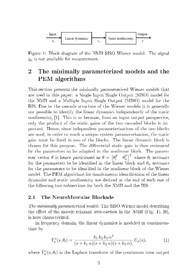
Figure 1: Block diagram of the NMB SISO Wiener model. The signalya is not available for measurement.

2 The minimally parameterized models and the

PEM algorithms

This section presents the minimally parameterized Wiener models thatare used in this paper: a Single Input Single Output (SISO) model forthe NMB and a Multiple Input Single Output (MISO) model for theBIS. Due to the cascade structure of the Wiener models it is generallynot possible to identify the linear dynamics independently of the staticnonlinearity, [1]. This is so because, from an input-output perspective,only the product of the static gains of the two cascaded blocks is im-portant. Hence, since independent parameterizations of the two blocksare used, in order to reach a unique system parameterization, the staticgain must be �xed in one of the blocks. The linear dynamic block ischosen for this purpose. The di�erential static gain is then estimatedby the parameters to be adapted in the nonlinear block. The param-eter vector θ is hence partitioned as θ =

[θTl θTn

]T where θl accountsfor the parameters to be identi�ed in the linear block and θn accountsfor the parameters to be identi�ed in the nonlinear block of the Wienermodel. The PEM algorithms for simultaneous identi�cation of the lineardynamics and static nonlinearity are derived at the end of each one ofthe following two subsections for both the NMB and the BIS.

2.1 The NeuroMuscular Blockade

The minimally parameterized model: The SISO Wiener model describingthe e�ect of the muscle relaxant atra-curium in the NMB (Fig. 1), [6],is here characterized.

In frequency domain, the linear dynamics is modeled in continuous-time by

Y ca (s, θl) =

k1 k2 k3 α3

(s+ k1 α)(s+ k2 α)(s+ k3 α),Ua(s), (1)

where Y ca (s, θl) is the Laplace transform of the continuous-time output

3

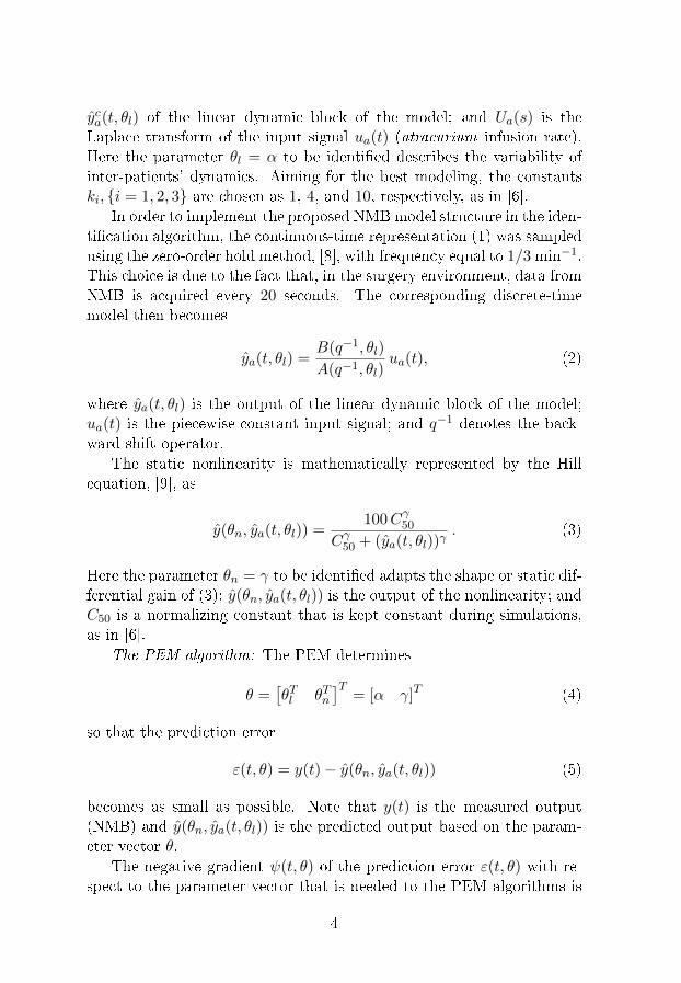
yca(t, θl) of the linear dynamic block of the model; and Ua(s) is theLaplace transform of the input signal ua(t) (atracurium infusion rate).Here the parameter θl = α to be identi�ed describes the variability ofinter-patients' dynamics. Aiming for the best modeling, the constantski, {i = 1, 2, 3} are chosen as 1, 4, and 10, respectively, as in [6].

In order to implement the proposed NMBmodel structure in the iden-ti�cation algorithm, the continuous-time representation (1) was sampledusing the zero-order hold method, [8], with frequency equal to 1/3 min−1.This choice is due to the fact that, in the surgery environment, data fromNMB is acquired every 20 seconds. The corresponding discrete-timemodel then becomes

ya(t, θl) =B(q−1, θl)

A(q−1, θl)ua(t), (2)

where ya(t, θl) is the output of the linear dynamic block of the model;ua(t) is the piecewise-constant input signal; and q−1 denotes the back-ward shift operator.

The static nonlinearity is mathematically represented by the Hillequation, [9], as

y(θn, ya(t, θl)) =100Cγ50

Cγ50 + (ya(t, θl))γ. (3)

Here the parameter θn = γ to be identi�ed adapts the shape or static dif-ferential gain of (3); y(θn, ya(t, θl)) is the output of the nonlinearity; andC50 is a normalizing constant that is kept constant during simulations,as in [6].

The PEM algorithm: The PEM determines

θ =[θTl θTn

]T= [α γ]T (4)

so that the prediction error

ε(t, θ) = y(t)− y(θn, ya(t, θl)) (5)

becomes as small as possible. Note that y(t) is the measured output(NMB) and y(θn, ya(t, θl)) is the predicted output based on the param-eter vector θ.

The negative gradient ψ(t, θ) of the prediction error ε(t, θ) with re-spect to the parameter vector that is needed to the PEM algorithms is

4

given by

ψ(t, θ) = −[∂ε(t, θ)

∂θ

]T=

[∂y(θn, ya(t, θl))

∂θ

]T(6)

=

[∂y(θn, ya(t, θl))

∂ya(t, θl)

∂ya(t, θl)

∂α

∂y(θn, ya(t, θl))

∂γ

]T.

The criterion to be minimized in the search, [10], is

V (θ) =1

N

N∑t=1

ε2(t, θ), (7)

where N is the total number of data points.The minimization of (7) is performed using the numerical Newton-

Raphson algorithm, [10],

θ(k+1) = θ(k) − β(V ′′(θ(k))

)−1V ′(θ(k))T , (8)

where θ(k) denotes the kth iteration in the search and β is a diagonalmatrix used to control the step length. The derivatives of V (θ) can befound as:

V ′(θ) = − 2

N

N∑t=1

εT (t, θ)ψT (t, θ) , (9)

V ′′(θ) =2

N

N∑t=1

ψ(t, θ) ψT (t, θ)− 2

N

N∑t=1

εT (t, θ)∂

∂θψT (t, θ)

≈ 2

N

N∑t=1

ψ(t, θ)ψT (t, θ) . (10)

The approximation in (10) is justi�ed in [10] and is supported by thefact that, at the global minimum point, ε(t, θ) becomes asymptoticallywhite noise which is independent of ψ(t, θ).

Regarding the linear block of the Wiener model, a projection al-gorithm is needed to keep the model asymptotically stable. For thispurpose, the poles of the transfer function (1) are monitored at every

5

iteration step by the use of the following projection algorithm for theparameter α:

α(k+1) =

{α(k+1), if α(k+1) > δ > 0

α(k), if α(k+1) ≤ δ(11)

For the nonlinear block (3), it is necessary to assure that γ does notreach negative values. The following projection algorithm was used forthe parameter γ:

γ(k+1) =

{γ(k+1), if γ(k+1) > δ > 0

γ(k), if γ(k+1) ≤ δ(12)

Both updates are hence stopped if the new parameter estimates are out-side the feasible region.

The PEM for the identi�cation of the NMB can be summarized usingthe formulas de�ned above:for k = 0 to K

θ = θ(k) ⇔[θTl θTn

]T=[θ

(k)l

T θ(k)n

T]T

ya(t, θl) =B(q−1, θl)

A(q−1, θl)ua(t)

y(θn, ya(t, θl)) =100C γ50

C γ50 + (ya(t, θl))γ

ε(t, θ) = y(t)− y(θn, ya(t, θl))

∂y(θn, ya(t, θl))

∂ya(t, θl)= −100C γ50 γ ya(t, θl)

γ−1

(C γ50 + ya(t, θl)γ)2

∂ya(t, θl)

∂α=ya(t, θl)

∣∣α=α+∆α

− ya(t, θl)∆α

∂y(θn, ya(t, θl))

∂γ=

100C γ50 log(C50)

C γ50 + ya(t, θl)γ− 100C γ50

(C γ50 + ya(t, θl)γ)2

×(

log(C50)C γ50 + log(ya(t, θl)) ya(t, θl)γ)

6

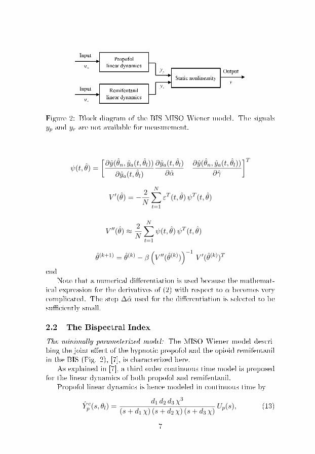
Figure 2: Block diagram of the BIS MISO Wiener model. The signalsyp and yr are not available for measurement.

ψ(t, θ) =

[∂y(θn, ya(t, θl))

∂ya(t, θl)

∂ya(t, θl)

∂α

∂y(θn, ya(t, θl))

∂γ

]T

V ′(θ) = − 2

N

N∑t=1

εT (t, θ)ψT (t, θ)

V ′′(θ) ≈ 2

N

N∑t=1

ψ(t, θ)ψT (t, θ)

θ(k+1) = θ(k) − β(V ′′(θ(k))

)−1V ′(θ(k))T

endNote that a numerical di�erentiation is used because the mathemat-

ical expression for the derivatives of (2) with respect to α becomes verycomplicated. The step ∆α used for the di�erentiation is selected to besu�ciently small.

2.2 The Bispectral Index

The minimally parameterized model: The MISO Wiener model descri-bing the joint e�ect of the hypnotic propofol and the opioid remifentanilin the BIS (Fig. 2), [7], is characterized here.

As explained in [7], a third-order continuous-time model is proposedfor the linear dynamics of both propofol and remifentanil.

Propofol linear dynamics is hence modeled in continuous-time by

Y cp (s, θl) =

d1 d2 d3 χ3

(s+ d1 χ) (s+ d2 χ) (s+ d3 χ)Up(s), (13)

7

where Y cp (s, θl) is the Laplace transform of the continuous-time output

ycp(s, θl) of the linear dynamic block of the model for propofol and Up(s)is the Laplace transform of the input signal up(t) (propofol infusion rate).The pole location χ is selected as the parameter to be identi�ed in (13).

Remifentanil linear dynamics is similarly modeled in continuous-timeby

Y cr (s, θl) =

l1 l2 l3 η3

(s+ l1 η) (s+ l2 η) (s+ l3 η)Ur(s), (14)

where Y cr (s, θl) is the Laplace transform of the continuous-time output

ycr(t, θl) of the linear dynamic block of the model for remifentanil andUr(s) is the Laplace transform of the input signal ur(t) (remifentanilinfusion rate). The pole location η is selected as the parameter to beidenti�ed in (14).

The constants di and li, {i = 1, 2, 3} were chosen as {d1 = 1, d2 =9, d3 = 10} and {l1 = 1, l2 = 2, l3 = 3}, having been determined by theuse of batch identi�cation over a di�erent database of real BIS data, [11].Consequently, the parameter vector θl becomes θl = [χ η]T .

In order to implement the proposed model structure in the PEMalgorithm, the continuous-time representations of (13) and (14) weresampled using the zero-order hold method, [8], with frequency of 1/12min−1. This value is dependent on the sampling rate of the measurementdevices of BIS. Consequently, the discrete-time outputs of the lineardynamic blocks for propofol and remifentanil are, respectively,

yp(t, θl) =D(q−1, θl)

C(q−1, θl)up(t) , (15)

yr(t, θl) =G(q−1, θl)

F (q−1, θl)ur(t) . (16)

Using as starting point the standard model of [12] that describes thee�ect of the interaction between propofol and remifentanil in the BIS, anew formulation for the nonlinearity was proposed in [7]:

y(θn, yp(t, θl), yr(t, θl)) =y0

1 +(yr(t,θl)EC50r

+myp(t,θl)EC50p

)ζ . (17)

Here θn = [m ζ]T ; m and ζ are the parameters to be identi�ed inthe nonlinearity; EC50p and EC50r are propofol and remifentanil nor-malizing constants, respectively, that were chosen in [7]; and y0 = 97.7is the baseline value for BIS.

8

The PEM algorithm: The PEM determines θ so that the predictionerror

ε(t, θ) = y(t)− y(θn, yp(t, θl), yr(t, θl)) (18)

becomes as small as possible. Note that y(t) is the measured output(BIS) and y(θn, yp(t, θl), yr(t, θl)) is the predicted output based on theparameter vector θ.

The gradient of the prediction error ε(t, θ) is given by

ψ(t, θ) = −[∂ε(t, θ)

∂θ

]T

=

∂y(θn,yp(t,θl),yr(t,θl))∂yp(t,θl)

∂yp(t,θl)∂χ

∂y(θn,yp(t,θl),yr(t,θl))∂yr(t,θl)

∂yr(t,θl)∂η

∂y(θn,yp(t,θl),yr(t,θl))∂m

∂y(θn,yp(t,θl),yr(t,θl))∂ζ

. (19)

The quadratic criterion (7) is used, being minimized by the Newton-Raphson algorithm (8). The derivatives of V (θ) are calculated using (9)and (10).

The restriction on the update of the estimates of χ and η are the sameas to α for the NMB in (11). The argument supporting this choice is thesame as before. Similarly, m and ζ follow the same projection algorithmof γ in (12). According to [12], the interaction between propofol andremifentanil is supradditive. As consequence, it is assumed that m in(17) is lower bounded by zero. For ζ the argument is the same as for γin (12). Both updates are hence stopped if the new parameter updatesare outside the feasible region.

The PEM for the identi�cation of BIS can be summarized using theformulas de�ned above:for k = 0 to K

θ = θ(k) ⇔[θTl θTn

]T=[θ

(k)l

T θ(k)n

T]T

yp(t, θl) =D(q−1, θl)

C(q−1, θl)up(t)

9

yr(t, θl) =G(q−1, θl)

F (q−1, θl)ur(t)

y(θn, yp(t, θl), yr(t, θl)) =y0

1 +(yr(t,θl)EC50p

+ myp(t,θl)EC50r

)ζε(t, θ) = y(t)− y(θn, yp(t, θl), yr(t, θl))

∂yp(t, θl)

∂χ=yp(t, θl)

∣∣χ=χ+∆χ

− yp(t, θl)∆χ

∂yr(t, θl)

∂η=yr(t, θl)

∣∣η=η+∆η

− yr(t, θl)∆η

ψ(t, θ) =

−y0 m ζ

(yr(t,θl)

EC50p+m

yp(t,θl)

EC50r

)ζ−1

(1+

(yr(t,θl)

EC50p+m

yp(t,θl)

EC50r

)ζ)2∂yp(t,θl)∂χ

−y0 ζ(yr(t,θl)

EC50r+m

yp(t,θl)

EC50p

)ζ−1

(1+

(yr(t,θl)

EC50r+m

yp(t,θl)

EC50p

)ζ)2∂yr(t,θl)

∂η

−y0yp(t,θl)

EC50pζ

(yr(t,θl)

EC50r+m

yp(t,θl)

EC50p

)ζ−1

(1+

(yr(t,θl)

EC50r+m

yp(t,θl)

EC50p

)ζ)2

−y0 log

(yr(t,θl)

EC50r+m

yp(t,θl)

EC50p

)(yr(t,θl)

EC50r+m

yp(t,θl)

EC50p

)ζ(

1+

(yr(t,θl)

EC50r+m

yp(t,θl)

EC50p

)ζ)2

V ′(θ) = − 2

N

N∑t=1

εT (t, θ)ψT (t, θ)

V ′′(θ) ≈ 2

N

N∑t=1

ψ(t, θ)ψT (t, θ)

10

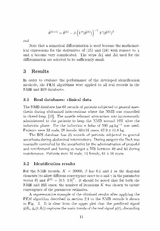
θ(k+1) = θ(k) − β(V ′′(θ(k))

)−1V ′(θ(k))T

endNote that a numerical di�erentiation is used because the mathemat-

ical expressions for the derivatives of (15) and (16) with respect to χand η become very complicated. The steps ∆χ and ∆η used for thedi�erentiation are selected to be su�ciently small.

3 Results

In order to evaluate the performance of the developed identi�cationmethods, the PEM algorithms were applied to all real records in theNMB and BIS databases.

3.1 Real databases: clinical data

The NMB database has 60 records of patients subjected to general anes-thesia during abdominal interventions where the NMB was controlledin closed-loop, [13]. The muscle relaxant atracurium was intravenouslyadministered to the patients to keep the NMB around 10% after theinduction phase. For the induction a bolus of 500 µg.kg−1 was used.Patients were 32 male, 28 female, 60±16 years, 67.9± 11.8 kg.

The BIS database has 25 records of patients subjected to generalanesthesia during abdominal interventions. During surgery the DoA wasmanually controlled by the anesthetist by the administration of propofoland remifentanil and having as target a BIS between 40 and 65 duringmaintenance. Patients were 10 male, 15 female, 61± 16 years.

3.2 Identi�cation results

For the NMB records, K = 20000, β has 0.1 and 1 as the diagonalelements (to allow di�erent convergence rates to α and γ in the parametervector θ) and θ(0) = [0.5 2.0]T . It should be noted that for both theNMB and BIS cases, the number of iterations K was chosen to ensureconvergence of the parameter estimates.

A representative example of the obtained results after applying thePEM algorithm described in section 2.1 to the NMB records is shownin Fig. 3. It is clear from the upper plot that the predicted signaly(θn, ya(t, θl)) captures the main trends of the real signal y(t), discarding

11

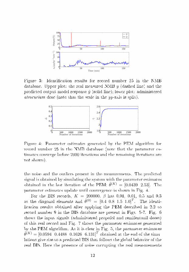
0 50 100 1500

25

50

75

100

Output(%)

0 50 100 1500

10

20...

500

Time (min)

ua(µgkg−1min

−1)

yy

Figure 3: Identi�cation results for record number 25 in the NMBdatabase. Upper plot: the real measured NMB y (dashed line) and thepredicted output model response y (solid line); lower plot: administeredatracurium dose (note that the scale in the yy-axis is split).

0 500 1000 1500 20000

0.1

0.2

0.3

0.4

0.5

Number of iterations

α

0 500 1000 1500 20001.8

2

2.2

2.4

2.6

Number of iterations

γ

Figure 4: Parameter estimates generated by the PEM algorithm forrecord number 25 in the NMB database (note that the parameter es-timates converge before 2000 iterations and the remaining iterations arenot shown).

the noise and the outliers present in the measurements. The predictedsignal is obtained by simulating the system with the parameter estimatesobtained in the last iteration of the PEM: θ(K) = [0.0439 2.53]. Theparameter estimates update until convergence is shown in Fig. 4.

For the BIS records, K = 200000, β has 0.01, 0.01, 0.5 and 0.3as the diagonal elements and θ(0) = [0.4 0.8 1.5 1.0]T . The identi-�cation results obtained after applying the PEM described in 2.2 torecord number 9 in the BIS database are present in Figs. 5-7. Fig. 6shows the input signals (administered propofol and remifentanil doses)of this real record and Fig. 7 shows the parameter estimates generatedby the PEM algorithm. As it is clear in Fig. 5, the parameter estimatesθ(K) = [0.0594 0.4488 0.1626 6.131]T obtained at the end of the simu-lations give rise to a predicted BIS that follows the global behavior of thereal BIS. Here the presence of noise corrupting the real measurements

12

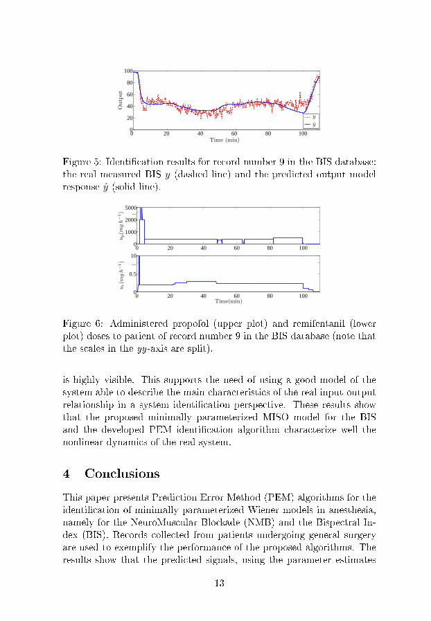
0 20 40 60 80 1000

20

40

60

80

100

Time (min)

Output

y

y

Figure 5: Identi�cation results for record number 9 in the BIS database:the real measured BIS y (dashed line) and the predicted output modelresponse y (solid line).

0 20 40 60 80 1000

1000

2000...

5000

up(m

gh−1)

0 20 40 60 80 1000

0.5

...10

Time(min)

ur(m

gh−1)

Figure 6: Administered propofol (upper plot) and remifentanil (lowerplot) doses to patient of record number 9 in the BIS database (note thatthe scales in the yy-axis are split).

is highly visible. This supports the need of using a good model of thesystem able to describe the main characteristics of the real input-outputrelationship in a system identi�cation perspective. These results showthat the proposed minimally parameterized MISO model for the BISand the developed PEM identi�cation algorithm characterize well thenonlinear dynamics of the real system.

4 Conclusions

This paper presents Prediction Error Method (PEM) algorithms for theidenti�cation of minimally parameterized Wiener models in anesthesia,namely for the NeuroMuscular Blockade (NMB) and the Bispectral In-dex (BIS). Records collected from patients undergoing general surgeryare used to exemplify the performance of the proposed algorithms. Theresults show that the predicted signals, using the parameter estimates

13

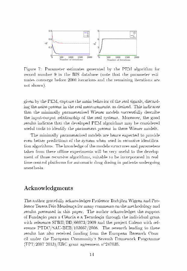
0 500 1000 1500 20000

0.3

0.6

0.9

Number of iterations

θ l

0 500 1000 1500 20000

3

6

9

Number of iterations

θ n

χη

mζ

Figure 7: Parameter estimates generated by the PEM algorithm forrecord number 9 in the BIS database (note that the parameter esti-mates converge before 2000 iterations and the remaining iterations arenot shown).

given by the PEM, capture the main behavior of the real signals, discard-ing the noise present in the real measurements, as desired. This indicatesthat the minimally parameterized Wiener models successfully describethe input-output relationship of the real systems. Moreover, the goodresults indicate that the developed PEM algorithms may be considereduseful tools to identify the parameters present in these Wiener models.

The minimally parameterized models are hence expected to provideeven better predictions of the system when used in recursive identi�ca-tion algorithms. The knowledge of the models structures and parameterstaken from these o�ine experiments will be very useful to the develop-ment of those recursive algorithms, suitable to be incorporated in real-time control platforms for automatic drug dosing in patients undergoinganesthesia.

Acknowledgments

The author gratefully acknowledges Professor Torbjörn Wigren and Pro-fessor Teresa Feio Mendonça for many comments on the methodology andresults presented in this paper. The author acknowledges the supportof Fundação para a Ciência e a Tecnologia through the individual grantwith reference SFRH/BD/60973/2009 and the project Galeno with ref-erence PTDC/SAU-BEB/103667/2008. The research leading to theseresults has also received funding from the European Research Coun-cil under the European Community's Seventh Framework Programme(FP7/2007-2013)/ERC grant agreement no247035.

14

References

[1] T. Wigren, �Recursive prediction error identi�cation method usingthe nonlinear Wiener model,� Automatica, vol. 29, no. 4, pp. 1011�1025, 1993.

[2] H. Derendorf and B. Meibohm, �Modeling of Pharmacoki-netic/Pharmacodynamic (PK/PD) relationships: concepts and per-spectives,� Pharmaceutical Research, vol. 16, pp. 176�185, 1999.

[3] T. Mendonça, J. Lemos, H. Magalhães, P. Rocha, and S. Esteves,�Drug delivery for neuromuscular blockade with supervised multi-model adaptive control,� IEEE Transactions on Control Systems

Technology, vol. 17, no. 6, pp. 1237 �1244, nov. 2009.

[4] J. Sigl and N. Chamoun, �An introduction to bispectral analysisfor the electroencephalogram,� Journal of Clinical Monitoring and

Computing, vol. 10, pp. 392�404, 1994.

[5] J. W. Johansen and P. S. Sebel, �Development and clinical applica-tion of electroencephalographic bispectrum monitoring,� Anesthesi-ology, vol. 93, pp. 1336�1344, 2000.

[6] M. M. Silva, T. Wigren, and T. Mendonça, �Nonlinear identi�cationof a minimal neuromuscular blockade model in anesthesia,� IEEE

Transactions on Control Systems Technology, 2011.

[7] M. M. Silva, T. Mendonça, and T. Wigren, �Online nonlinear iden-ti�cation of the e�ect of drugs in anaesthesia using a minimal pa-rameterization and BIS measurements,� in Proc. American Control

Conference (ACC'10), Baltimore, USA, June 2010, pp. 4379�4384.

[8] K. J. Åström and B. Wittenmark, Computer-Controlled Systems.Englewood Cli�s, NJ: Prentice Hall, 1984.

[9] B. Weatherley, S. Williams, and E. Neill, �Pharmacokinetics, phar-macodynamics and dose-response relationships of atracurium ad-ministered i. v.� Br. J. Anaesth., vol. 55, pp. 39s�45s, 1983.

[10] T. Söderström and P. Stoica, System Identi�cation. Hemel Hemp-stead, UK: Prentice-Hall, 1989.

15

[11] M. M. Silva, T. Wigren, and T. Mendonça, �Nonlinear iden-ti�cation of the human response to anaesthesia by the useof BIS measurements,� Dept. Information Technology, UppsalaUniversity, Uppsala, Sweden, Tech. Rep. 2010-008, Available:http://www.it.uu.se/research/publications/reports/, Mar. 2010.

[12] C. F. Minto, T. W. Schnider, T. G. Short, K. M. Gregg, A. Gen-tilini, and S. L. Shafer, �Response surface model for anesthetic druginteractions,� Anesthesiology, vol. 92, pp. 1603�1616, 2000.

[13] T. Mendonça, H. Magalhães, P. Lago, and S. Esteves, �Hipocrates:a robust system for the control of neuromuscular blockade,� Journalof Clinical Monitoring and Computing, vol. 18, pp. 265�273, 2004.

16

Paper IV

Nonlinear adaptive control of the

NeuroMuscular Blockade in anesthesia

Margarida M. Silva, Teresa Mendonça and Torbjörn Wigren

Abstract

This paper presents a nonlinear adaptive control strategy basedon the Wiener model for control of the NeuroMuscular Blockadein anesthesia. The structure combines the inversion of the staticnonlinearity present in the Wiener model with a pole-placementcontroller for the linearized system. The overall strategy exploitsidenti�cation of a minimally parameterized model for the descrip-tion of the e�ect of the muscle relaxant atracurium in the Neu-roMuscular Blockade. An Extended Kalman Filter was developedfor that purpose, providing estimates of the model parameters forboth the linear controller and the blocks where the inversion of thestatic linearity is performed. Simulations were run in a databaseof 100 patients simulated with the standard physiologically-basedpharmacokinetic/pharmacodynamic model for the NeuroMuscularBlockade. The results show that the nonlinear adaptive controllerperforms well regarding reference following and tackles changes inthe patient's dynamics. Noisy scenarios were also simulated to testthe robustness of the proposed strategy.

1 Introduction

Regardless of the �eld of application, the development of any controlstrategy comprises several main tasks, namely, system modeling, designof a control law, implementation and validation. Having a good mathe-matical model of the system becomes more and more important as thecomplexity of the system to be controlled increases. In biomedical appli-cations, due to the strong parameter variability from patient to patientthis requirement is particularly demanding. Moreover, since the patientdynamics may change during the time-course of the control action, anadaptive control strategy is a natural choice when dealing with controlof a particular human response to external or internal excitation.

This paper presents a nonlinear adaptive control strategy, based onthe Wiener model, for control of the NeuroMuscular Blockade (NMB)in anesthesia. The Wiener model consists of linear dynamics in cascadewith a static nonlinear function [1]. In the anesthesia �eld this structureis frequently present when modeling the e�ect of drug administration inthe human body e.g. for the NMB or the Bispectral Index (BIS). Accor-ding to this structure an initial dynamic mixing of the administered drugis present in the di�erent theoretical compartments of the human body[2], being followed by a static transduction from the concentration of thedrug in the e�ect site to the observed clinical e�ect [3]. Even thoughnonlinear, some advantages result from the fact that the nonlinearity isstatic. In particular, in controllers for Wiener type models a commonstrategy is to apply the inverse of the nonlinearity to the reference signaland to the measured output signal, and to design linear controllers forthe obtained signals afterwards [4]. The main contribution of this paperpresents a combination of this structure with adaptivity. The overallstrategy also exploits the recursive identi�cation of a new minimally pa-rameterized model for the e�ect of the muscle relaxant atracurium inthe NMB [5, 6]. This is of central importance since the excitation prop-erties of the input (atracurium dose pro�le) are known to be poor andthe number of output datapoints (NMB measurements) is small. Goodresults are expected to be achieved with this strategy since the maindrawback of identifying and controlling an overparameterized model isnot present.

Section 2 describes the NMB minimally parameterized model usedfor the system modeling and the identi�cation strategy, an ExtendedKalman Filter (EKF). Section 3 presents the main features of the adap-tive control strategy while section 4 shows the results of running theproposed strategy in a database of 100 simulated patients. Section 5draws the conclusions.

2 The model and the identi�cation algorithm

2.1 The minimally parameterized model for the NMB

A Single Input Single Output (SISO) nonlinear Wiener model (Fig. 1)describing the e�ect of the muscle relaxant atracurium in the NMB ispresented here. It should be emphasized that the choice of this modelwith a minimal number of parameters to model the relationship betweenthe drug and the measured e�ect is crucial for the success of the present

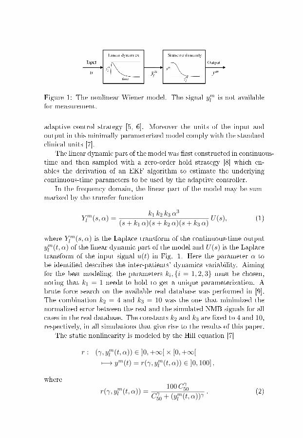
Figure 1: The nonlinear Wiener model. The signal yml is not availablefor measurement.

adaptive control strategy [5, 6]. Moreover the units of the input andoutput in this minimally parameterized model comply with the standardclinical units [7].

The linear dynamic part of the model was �rst constructed in continuous-time and then sampled with a zero-order hold strategy [8] which en-ables the derivation of an EKF algorithm to estimate the underlyingcontinuous-time parameters to be used by the adaptive controller.

In the frequency domain, the linear part of the model may be sum-marized by the transfer function

Y ml (s, α) =

k1 k2 k3 α3

(s+ k1 α)(s+ k2 α)(s+ k3 α)U(s), (1)

where Y ml (s, α) is the Laplace transform of the continuous-time output

yml (t, α) of the linear dynamic part of the model and U(s) is the Laplacetransform of the input signal u(t) in Fig. 1. Here the parameter α tobe identi�ed describes the inter-patients' dynamics variability. Aimingfor the best modeling, the parameters ki, {i = 1, 2, 3} must be chosen,noting that k1 = 1 needs to hold to get a unique parameterization. Abrute force search on the available real database was performed in [9].The combination k2 = 4 and k3 = 10 was the one that minimized thenormalized error between the real and the simulated NMB signals for allcases in the real database. The constants k2 and k3 are �xed to 4 and 10,respectively, in all simulations that give rise to the results of this paper.

The static nonlinearity is modeled by the Hill equation [7]

r : (γ, yml (t, α)) ∈ ]0,+∞[× [0,+∞[

7−→ ym(t) = r(γ, yml (t, α)) ∈ ]0, 100] ,

where

r(γ, yml (t, α)) =100Cγ50

Cγ50 + (yml (t, α))γ. (2)

Here γ is the parameter to be identi�ed; r(·, ·) is a known staticnonlinear function; ym(t) is the output of the nonlinearity; yml (t, α) is thecontinuous-time output of the linear dynamic part of the model (1); andC50 is a normalizing constant that is kept constant during simulations,similarly to [5].

Due to the Wiener model cascade structure, and as stressed in [1],only the product of the small signal static gains of the two cascadedblocks is important from an input-output point of view. Noting thatthe linear part (1) contributes with a unity gain for the whole system,the di�erential static gain must be estimated by the parameter γ to beadapted in the nonlinear part (2). At the same time, γ adapts the shapeor nonlinear static di�erential gain of (2). The parameter vector to beidenti�ed in the EKF structure is then selected as θ = [α γ] T . Henceonly two parameters are estimated.

2.2 Identi�cation: the EKF algorithm

In order to implement the model structure (1), (2) in the EKF algorithm,the continuous-time representation (1) was sampled using a zero-orderhold method [8].

The discrete-time model becomes{x(kh+ h) = Φ(α)x(kh) + Γ(α)u(kh)yml (kh, α) = C(α)x(kh)

, (3)

whereΦ(α) = eA(α)h

Γ(α) =∫ h0 e

A(α)s dsB(α). (4)

Here, u(kh) ∈ R is the input (piecewise constant atracurium dose),x(kh) ∈ R3×1 is the discrete-time state-vector, yml (kh, α) ∈ R is thediscrete-time output of the linear block, Φ(α) ∈ R3×3 and Γ(α) ∈ R3×1

are the sampled system matrices, and A(α) ∈ R3×3 and B(α) ∈ R3×1 arethe continuous-time system matrices. Note that the k′is, {i = 1, 2, 3} arenot shown explicitly in (3) since they are �xed in the simulations, priorto (2). Due to the fact that in the surgery environment, data from NMBis monitored and acquired every 20 seconds to ensure that all the nerve�bers are recruited every time a electrical stimulation is performed, thezero-order hold method is applied using h = 1/3 min−1.

The sampling does not a�ect the nonlinear block, hence (2) can be

used as it is. The model output is then given by:

ym(kh) = r(γ, yml (kh, α)) =100Cγ50

Cγ50 + (yml (kh, α))γ. (5)

To describe the EKF, the underlying general discrete-time nonlinearmodel is assumed to be

x(t+ 1) = f(t, x(t), u(t)) + g(t, x(t)) v(t)

y(t) = h(t, x(t)) + e(t) , (6)

where v(t) and e(t) are mutually independent Gaussian white noise se-quences with zero means and covariances R1(t) and R2(t), respectively.The EKF algorithm can then be summarized as follows (cf. e.g. [10]):

H(t) =∂h(t, x)

∂x

∣∣∣∣x=x(t|t−1)

K(t) = P (t|t− 1)HT (t)

× [H(t)P (t|t− 1)HT (t) +R2(t)]−1

x(t|t) = x(t|t− 1) +K(t)[y(t)− h(t, x(t|t− 1))]

P (t|t) = P (t|t− 1)−K(t)H(t)P (t|t− 1)

x(t+ 1|t) = f(t, x(t|t), u(t))

F (t) =∂f(t, x)

∂x

∣∣∣∣x=x(t|t)

(7)

G(t) = g(t, x)∣∣x=x(t|t)

P (t+ 1|t) = F (t)P (t|t)F T (t) +G(t)R1(t)GT (t)

To enable the estimation of the model parameters with the EKF, acoupled identi�cation model is de�ned. The model merges the sampledmodel (3) and a random walk model for the parameter estimates [11].The resulting augmented state vector (denoted by x) becomes

x(kh) = [x1(kh) x2(kh) x3(kh) α(kh) γ(kh)]T . (8)

Using (8), the extended state-space model is the following:

x(kh+ h) =

[Φ(α(kh)) 03×2

02×3 I

]x(kh)α(kh)γ(kh)

+

+

[Γ(α(kh))

02×1

]u(kh) +

vx(kh)vα(kh)vγ(kh)

≡

f1(kh, x(kh), u(kh))...

f5(kh, x(kh), u(kh))

+ v(kh)

≡ f(kh, x(kh), u(kh)) + v(kh) , (9)

ym(kh) =100C

γ(kh)50

Cγ(kh)50 + (C(α(kh))x(kh))γ(kh)

+ e(kh)

≡ h(kh, x(kh)) + e(kh) , (10)

C(·) = [C(·) 0 0] . (11)

In the EKF algorithm structure (7) it is necessary to linearize both f(t, x)and h(t, x). The linearization of f(kh, x(kh), u(kh)) in (9) was performedanalytically. The formula for F (kh) is not shown here due to its complex-ity. The linearization of h(kh, x(kh)) in (10) was performed numericallyin order to reduce the computational complexity of the calculations:

H(kh) =h(kh, x(kh) + ∆x(kh))− h(kh, x(kh))

∆x(kh),

where ∆x(kh) is the step for the di�erentiation and is chosen to be small.

3 The adaptive controller

3.1 Structure

The structure of the adaptive controller proposed in this paper is shownin Fig. 2 and comprises three main tasks that are performed by order ateach time step: online identi�cation of the model parameters by the EKF,inversion of the nonlinearity using the current estimate of the nonlinearparameter and linear adaptive control. The use of the online identi�edmodel parameters to linearize the Wiener model and to calculate thelinear control law determines the adaptivity nature of this controller.

3.2 Inversion

Both the measured NMB from the patient (output y) and the referencevalue yref are �rst inverted through r−1(·, ·) [4] using the current esti-mate of γ provided by the EKF identi�cation block. It should be stressed

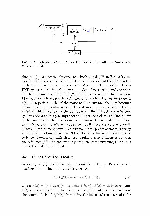
Figure 2: Adaptive controller for the NMB minimally parameterizedWiener model.

that r(·, ·) is a bijective function and both y and yref in Fig. 2 lay in-side [0, 100] as consequence of monitoring restrictions of the NMB in theclinical practice. Moreover, as a result of a projection algorithm in theEKF structure [5], γ is also lower-bounded. Due to this, and consider-ing the domains a�ecting r(·, ·) (2), no problems arise in this inversion.Ideally, when γ is accurately estimated and no disturbances are present,r(γ, ·) is a perfect model of the static nonlinearity and the loop becomeslinear. The static nonlinearity of the system is then canceled exactly byr−1(γ, ·) which means that the output of the linear block of the Wienersystem appears directly as input for the linear controller. The linear partof the controller is therefore designed to control the output of the lineardynamic part of the Wiener type system as if there was no static nonli-nearity. For the linear control a continuous-time pole placement strategywith integral action is used [4]. This allows the linearized control errorto be regulated away. This then also regulates away di�erences betweenthe reference yref and the output y since the same inverting function isapplied to both these signals.

3.3 Linear Control Design

According to (1), and following the notation in [4], pp. 93, the patientcontinuous-time linear dynamics is given by

A(s) yml (t) = B(s)u(t) + w(t) , (12)

where A(s) = (s + k1 α)(s + k2 α)(s + k3 α), B(s) = k1 k2 k3 α3, and

w(t) is a disturbance. The idea is to require that the response fromthe command signal yrefl (t) (here being the linear reference signal to be

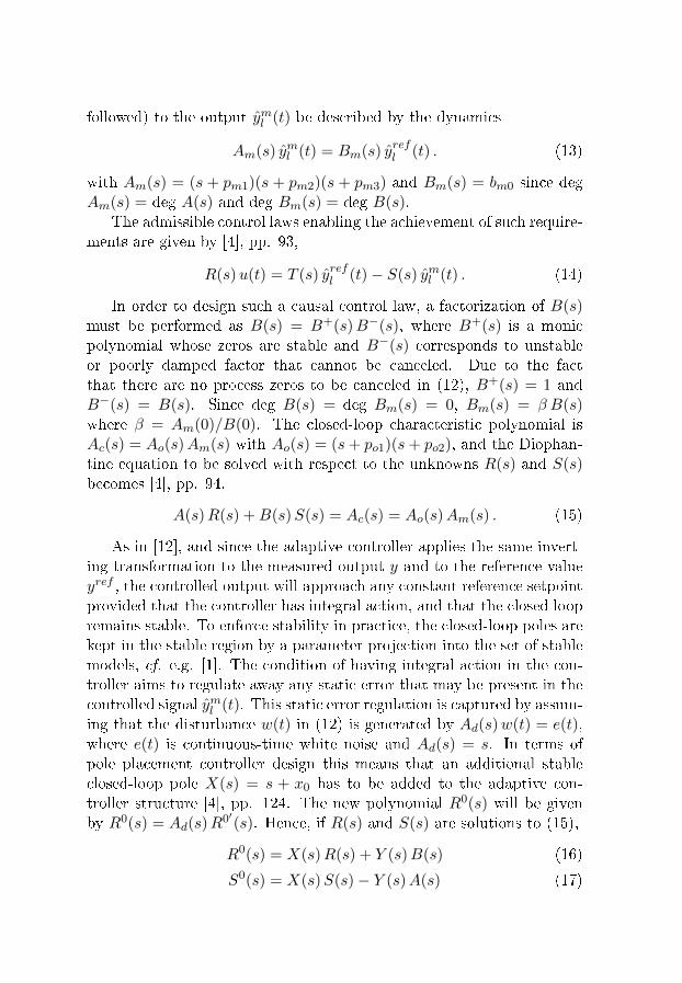
followed) to the output yml (t) be described by the dynamics

Am(s) yml (t) = Bm(s) yrefl (t) . (13)

with Am(s) = (s + pm1)(s + pm2)(s + pm3) and Bm(s) = bm0 since degAm(s) = deg A(s) and deg Bm(s) = deg B(s).

The admissible control laws enabling the achievement of such require-ments are given by [4], pp. 93,

R(s)u(t) = T (s) yrefl (t)− S(s) yml (t) . (14)

In order to design such a causal control law, a factorization of B(s)must be performed as B(s) = B+(s)B−(s), where B+(s) is a monicpolynomial whose zeros are stable and B−(s) corresponds to unstableor poorly damped factor that cannot be canceled. Due to the factthat there are no process zeros to be canceled in (12), B+(s) = 1 andB−(s) = B(s). Since deg B(s) = deg Bm(s) = 0, Bm(s) = β B(s)where β = Am(0)/B(0). The closed-loop characteristic polynomial isAc(s) = Ao(s)Am(s) with Ao(s) = (s+ po1)(s+ po2), and the Diophan-tine equation to be solved with respect to the unknowns R(s) and S(s)becomes [4], pp. 94,

A(s)R(s) +B(s)S(s) = Ac(s) = Ao(s)Am(s) . (15)

As in [12], and since the adaptive controller applies the same invert-ing transformation to the measured output y and to the reference valueyref , the controlled output will approach any constant reference setpointprovided that the controller has integral action, and that the closed loopremains stable. To enforce stability in practice, the closed-loop poles arekept in the stable region by a parameter projection into the set of stablemodels, cf. e.g. [1]. The condition of having integral action in the con-troller aims to regulate away any static error that may be present in thecontrolled signal yml (t). This static error regulation is captured by assum-ing that the disturbance w(t) in (12) is generated by Ad(s)w(t) = e(t),where e(t) is continuous-time white noise and Ad(s) = s. In terms ofpole placement controller design this means that an additional stableclosed-loop pole X(s) = s + x0 has to be added to the adaptive con-troller structure [4], pp. 124. The new polynomial R0(s) will be givenby R0(s) = Ad(s)R

0′(s). Hence, if R(s) and S(s) are solutions to (15),

R0(s) = X(s)R(s) + Y (s)B(s) (16)

S0(s) = X(s)S(s)− Y (s)A(s) (17)

will satisfy [4], pp. 123,

A(s)R0(s) +B(s)S0(s) = X(s)Ac(s) . (18)

From (16) it follows that

R0(s) = sR0′(s) = (s+ x0)R(s) + y0B(s) , (19)

with x0 to be chosen and Y (s) = y0 obtained by making s = 0 in (19):

y0 = −x0R(0)

B(0). (20)

Inserting X(s) and y0 into (16) and (17) the new controller is found.The complete control law is then given by

R0(s)u(t) = T (s) yrefl (t)− S0(s) yml (t) , (21)

resulting in a closed-loop system of order 6.

3.4 Anti-windup

Due to the nature of the problem to be solved, u(t) must be nonnega-tive and below a prede�ned maximum umax. Moreover, knowing thatcontrollers with integral action may perform poorly in the presence ofactuators that saturate [4], pp. 128, the control law (21) was furtheraugmented with an anti-windup strategy (depicted in Fig. 2). Rewrit-ing (21) in the observer form and describing the saturation in the inputas

u(t) =

0, if u(t) < 0

u(t), if 0 ≤ u(t) ≤ umax ,umax, if u(t) > umax

(22)

the control law avoiding windup is then given by [4], pp. 456,

A0(s)u(t) = T (s) yrefl (t)− S0(s) yml (t) (23)

+(A0(s)−R0(s))u(t) .

The control law (23) was discretized using the zero-order hold methodin [8] to obtain the drug dose to be given to the simulated patient in eachtime instant.

4 Simulation results

A number of simulations were carried out to test the performance ofthe proposed nonlinear adaptive controller. Each simulated patient waschosen from a bank of 100 models that was randomly generated in [13] as-suming a lognormal probability distribution for the 8 parameters presentin the standard physiologically-based Pharmacokinetic/Pharmacodynamic(PK/PD) model. Following clinical procedures, a bolus of atracurium(500µg kg−1) was assumed to be given to each simulated patient at t = 0min, making the NMB to drop from its initial value of 100% to a valuearound 0% in less than 10 minutes after administration.

The design of the adaptive strategy is such that the controller is onlyturned on at the beginning of the recovery from the initial bolus (t ≈ 30min [14]). This patient-dependent time instant is calculated online bythe OnLine tuned Algorithm for Recovery Detection [15] that is coupledto the adaptive controller structure (not shown in Fig. 2).

For simulation purposes, the EKF is initialized as in [6] with

x(0| − 1) = [0 0 0 0.03 1]T . (24)

The value of R2 is chosen as di�erent from [6] and varies dependingon the scenario for simulation, among the three that were tested.

Example 1: The �rst scenario assesses the nonlinear adaptive con-troller performance in a noiseless situation. Here R2 = 103. The refer-ence pro�le yref (t) to be followed is a square wave of amplitude 0.5%around the setpoint of 10% with period equal to 60π. Some simulationresults for case number 98 in the database for this �rst scenario are pre-sented in Fig. 3. The roots of polynomials Am(s), Ao(s) and X(s) arechosen such that the output signal of all cases in the database behavesimilarly and are −0.7, −0.6, −0.3, −0.8, −0.4, and −0.8, respectively.In Fig. 3(a) and 3(b) it is clear that the output signal y(t) follows thereference yref (t). The static error present at the beginning of the sim-ulation is regulated away with time, as expected due to the presenceof integral action in the controller. This reference tracking is possibledue to the control signal shown in Fig. 3(c). The peaks of dose existwhenever the reference changes, being in the admissible range of drugadministration for atracurium. The parameter estimates for this case,calculated by the EKF are shown in Fig. 3(d) and 3(e).

Example 2: The adaptive capability of the designed adaptive con-troller is evaluated in the second simulation scenario. The parametersof the standard physiologically-based PK/PD model of case number 98

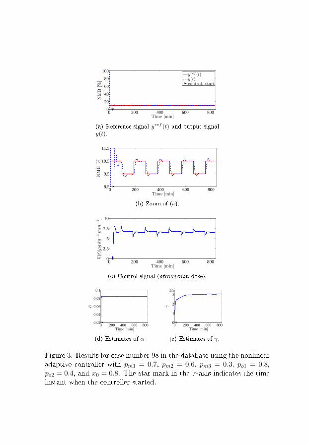
0 200 400 600 8000

20

40

60

80

100

Time [min]

NMB

[%]

yref (t)y(t)control. start

(a) Reference signal yref (t) and output signaly(t).

0 200 400 600 8008.5

9.5

10.5

11.5

Time [min]

NMB

[%]

(b) Zoom of (a).

0 200 400 600 8000

2.5

5

7.5

10

Time [min]

u(t)[µgkg−1min

−1]

(c) Control signal (atracurium dose).

0 200 400 600 8000.02

0.04

0.06

0.08

0.1

α

Time [min]

(d) Estimates of α.

0 200 400 600 8000

1

2

33.5

Time [min]

γ

(e) Estimates of γ.

Figure 3: Results for case number 98 in the database using the nonlinearadaptive controller with pm1 = 0.7, pm2 = 0.6, pm3 = 0.3, po1 = 0.8,po2 = 0.4, and x0 = 0.8. The star mark in the x -axis indicates the timeinstant when the controller started.

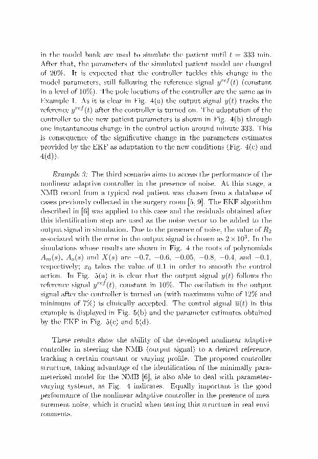
in the model bank are used to simulate the patient until t = 333 min.After that, the parameters of the simulated patient model are changedof 20%. It is expected that the controller tackles this change in themodel parameters, still following the reference signal yref (t) (constantin a level of 10%). The pole locations of the controller are the same as inExample 1. As it is clear in Fig. 4(a) the output signal y(t) tracks thereference yref (t) after the controller is turned on. The adaptation of thecontroller to the new patient parameters is shown in Fig. 4(b) throughone instantaneous change in the control action around minute 333. Thisis consequence of the signi�cative change in the parameters estimatesprovided by the EKF as adaptation to the new conditions (Fig. 4(c) and4(d)).

Example 3: The third scenario aims to access the performance of thenonlinear adaptive controller in the presence of noise. At this stage, aNMB record from a typical real patient was chosen from a database ofcases previously collected in the surgery room [5, 9]. The EKF algorithmdescribed in [6] was applied to this case and the residuals obtained afterthis identi�cation step are used as the noise vector to be added to theoutput signal in simulation. Due to the presence of noise, the value of R2

associated with the error in the output signal is chosen as 2×103. In thesimulations whose results are shown in Fig. 4 the roots of polynomialsAm(s), Ao(s) and X(s) are −0.7, −0.6, −0.05, −0.8, −0.4, and −0.1,respectively; x0 takes the value of 0.1 in order to smooth the controlaction. In Fig. 5(a) it is clear that the output signal y(t) follows thereference signal yref (t), constant in 10%. The oscilation in the outputsignal after the controller is turned on (with maximum value of 12% andminimum of 7%) is clinically accepted. The control signal u(t) in thisexample is displayed in Fig. 5(b) and the parameter estimates obtainedby the EKF in Fig. 5(c) and 5(d).

These results show the ability of the developed nonlinear adaptivecontroller in steering the NMB (output signal) to a desired reference,tracking a certain constant or varying pro�le. The proposed controllerstructure, taking advantage of the identi�cation of the minimally para-meterized model for the NMB [6], is also able to deal with parameter-varying systems, as Fig. 4 indicates. Equally important is the goodperformance of the nonlinear adaptive controller in the presence of mea-surement noise, which is crucial when testing this structure in real envi-ronments.

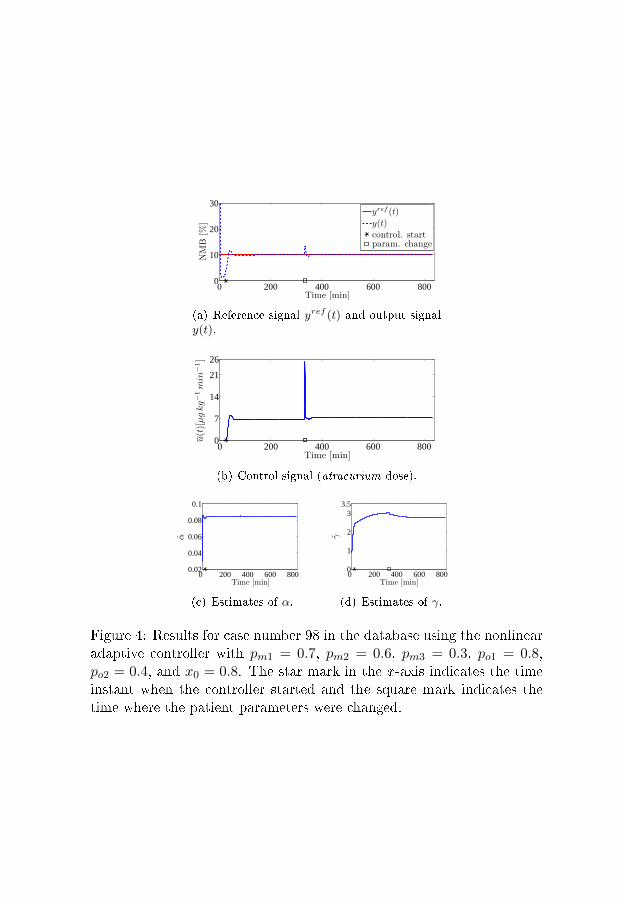
0 200 400 600 8000

10

20

30

Time [min]

NMB

[%]

yref (t)

y(t)

control. startparam. change

(a) Reference signal yref (t) and output signaly(t).

0 200 400 600 8000

7

14

21

26

Time [min]

u(t)[µgkg−1min

−1]

(b) Control signal (atracurium dose).

0 200 400 600 8000.02

0.04

0.06

0.08

0.1

Time [min]

α

(c) Estimates of α.

0 200 400 600 8000

1

2

33.5

Time [min]

γ

(d) Estimates of γ.

Figure 4: Results for case number 98 in the database using the nonlinearadaptive controller with pm1 = 0.7, pm2 = 0.6, pm3 = 0.3, po1 = 0.8,po2 = 0.4, and x0 = 0.8. The star mark in the x -axis indicates the timeinstant when the controller started and the square mark indicates thetime where the patient parameters were changed.

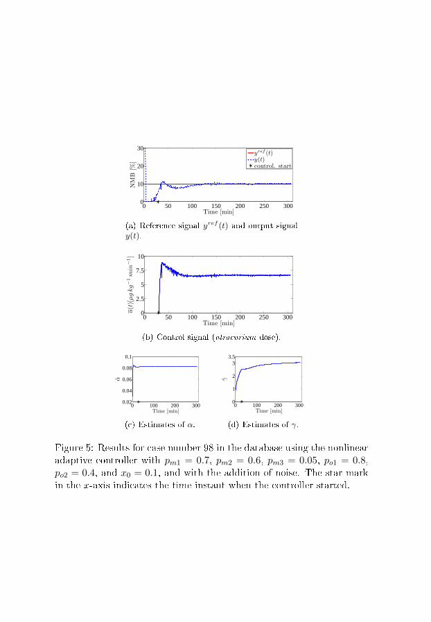
0 50 100 150 200 250 3000

10

20

30

Time [min]

NMB

[%]

yref (t)y(t)control. start

(a) Reference signal yref (t) and output signaly(t).

0 50 100 150 200 250 3000

2.5

5

7.5

10

Time [min]

u(t)[µgkg−1min

−1]

(b) Control signal (atracurium dose).

0 100 200 3000.02

0.04

0.06

0.08

0.1

α

Time [min]

(c) Estimates of α.

0 100 200 3000

1

2

33.5

Time [min]

γ

(d) Estimates of γ.

Figure 5: Results for case number 98 in the database using the nonlinearadaptive controller with pm1 = 0.7, pm2 = 0.6, pm3 = 0.05, po1 = 0.8,po2 = 0.4, and x0 = 0.1, and with the addition of noise. The star markin the x -axis indicates the time instant when the controller started.

5 Conclusions and future work

Even though many di�erent strategies for the control of the NeuroMus-cular Blockade have been developed, analyzed and implemented both insimulation and in real clinical situations during the past years e.g. [13],[16], [17], the features of the problem mainly the high inter- and intra-patient variability and the restrictions imposed by the clinical practicesuggest the development of di�erent approaches.

The novelty of the strategy proposed in this paper is the use of a min-imally parameterized model for the description of the e�ect of the musclerelaxant atracurium in the NeuroMuscular Blockade [6] and the incorpo-ration of an online identi�cation strategy (an Extended Kalman Filter)in the controller structure, providing adaptivity to the nonlinear con-troller. As a consequence the variability of the patient parameters doesnot interfere with the performance of the controller. Moreover, this newstrategy constitutes one reliable alternative to the use of a �nite num-ber of patient models to switch from [17]. Since stability conditions aremonitored by the Extended Kalman Filter, the controller is hence able tocover a continuous-range of patient nonlinear behaviors. It should alsobe stressed that the proposed adaptive controller addresses the controlof the NeuroMuscular Blockade in a highly realistic scenario, exempli�edby the third scenario of simulation where noise present in a real recordcollected in the surgery room is added to the output signal. The goodresults obtained in simulation are strong indications that the proposednonlinear adaptive controller will behave well when implemented in areal control situation.

In order to guarantee total patient safety and before implementingthis adaptive control strategy in real control platform, further work hasto be developed to screen convergence and stability properties of theproposed closed-loop structure. This nonlinear adaptive controller is alsohighly promising when extended to other nonlinear Wiener responses inanesthesia, namely the Bispectral Index.

Acknowledgments

The authors gratefully acknowledge the support of Fundação para a Ciên-cia e a Tecnologia through the individual grant with reference SFRH/BD/60973/2009 and the project Galeno with reference PTDC/SAU-BEB/103667/2008. The research leading to these results has also received

funding from the European Research Council under the European Com-munity's Seventh Framework Programme (FP7/2007-2013)/ERC grantagreement no247035.

References

[1] T. Wigren, �Recursive prediction error identi�cation method usingthe nonlinear Wiener model,� Automatica, vol. 29, no. 4, pp. 1011�1025, 1993.

[2] K. Godfrey, Compartmental models and their application. AcademicPress, 1983.

[3] H. Derendorf and B. Meibohm, �Modeling of pharmacoki-netic/pharmacodynamic (PK/PD) relationships: Concepts and per-spectives,� Pharmaceutical Research, vol. 16, pp. 176�185, 1999.

[4] K. J. Åström and B. Wittenmark, Adaptive Control, 2nd ed. Mi-neola, New York, USA: Dover Publications, Inc., 2008.

[5] M. M. Silva, T. Wigren, and T. Mendonça, �Nonlinearidenti�cation of a minimal neuromuscular blockade modelin anaesthesia,� Dept. Information Technology, Uppsala Uni-versity, Uppsala, Sweden, Tech. Rep. 2009-023, Available:http://www.it.uu.se/research/publications/reports/, Sept. 2009.

[6] ��, �Nonlinear identi�cation of a minimal neuromuscular blockademodel in anesthesia,� IEEE Trans. Contr. Sys. Tech. (in press), Jan.2011.

[7] B. Weatherley, S. Williams, and E. Neill, �Pharmacokinetics, phar-macodynamics and dose-response relationships of atracurium ad-ministered i. v.� Br. J. Anaesth., vol. 55, pp. 39s�45s, 1983.

[8] K. J. Åström and B. Wittenmark, Computer-Controlled Systems.Englewood Cli�s, NJ: Prentice Hall, 1984.

[9] M. M. Silva, �Prediction error identi�cation of minimally paramete-rized nonlinear Wiener models in anesthesia,� in Proc. of the 18th

IFAC World Congress (accepted), Milan, Italy, Aug 28-Sep 2 2010.

[10] T. Söderström, Discrete-time Stochastic Systems. London, UK:Springer-Verlag, 2002.

[11] T. Söderström and P. Stoica, System Identi�cation. Hemel Hemp-stead, UK: Prentice-Hall, 1989.

[12] T. Wigren and L. Brus, �Reduction of amplitude dependent gainvariations in control of non-linear Wiener type systems,� in Proc. of

the 7th IFAC Symposium on Nonlinear Control Systems, Pretoria,South Africa, 2007, pp. 730�735.

[13] P. Lago, T. Mendonça, and L. Gonçalves, �On-line autocalibrationof a PID controller of neuromuscular blockade,� in Proc. of the 1998

IEEE Inter. Conf. on Control Applications, Trieste, Italy, 1998, pp.363�367.

[14] H. Mellingho�, L. Radbruch, C. Diefenbach, and W. Buzello, �Acomparison of cisatracurium and atracurium: onset of neuromuscu-lar block after bolus injection and recovery after subsequent infu-sion,� Anesthesia & Analgesia, vol. 83, no. 5, pp. 1072�1075, 1996.

[15] M. M. Silva, C. Sousa, R. Sebastião, J. Gama, T. Mendonça,P. Rocha, and S. Esteves, �Total mass TCI driven by parametric es-timation,� in Proc. of the 17th Mediterranean Conference on Control

and Automation (MED'09), jun. 2009, pp. 1149�1154.

[16] P. Oliveira, J. P. Hespanha, J. M. Lemos, and T. Mendonça, �Super-vised multi-model adaptive control of neuromuscular blockade witho�-set compensation,� in Proc. of the 2009 European Contr. Conf.

(ECC'09), Aug. 2009, pp. 3064�3069.

[17] T. Mendonça, J. M. Lemos, H. Magalhães, P. Rocha, and S. Es-teves, �Drug delivery for neuromuscular blockade with supervisedmultimodel adaptive control,� IEEE Transactions on Control Sys-

tems Technology, vol. 17, no. 6, pp. 1237 �1244, nov. 2009.

Paper V

Exactly linearizing adaptive control of

propofol and remifentanil using a reduced

Wiener model for the depth of anesthesia

Margarida M. Silva, Torbjörn Wigren and Teresa Mendonça

Abstract

A closed-loop adaptive controller for propofol and remifentanil

administration using BIS measurements is proposed in this paper.

The controller design relies on a reduced MISO Wiener model for

the depth of anesthesia. The exact linearization of this minimal

Wiener structure using the model continuous-time parameter es-

timates calculated online by an extended Kalman �lter is a key

point in the design. A linear quadratic gaussian controller is devel-

oped for the exactly linearized system. Good results were obtained

when the robustness of the proposed controller was assessed with

respect to inter and intrapatient variability through Monte Carlo

simulations on a database of 500 patients.

1 Introduction

This paper presents an exactly linearizing adaptive controller for thedepth of anesthesia (DoA) based on the reduced Wiener model proposedin [1]. The controlled inputs are propofol and remifentanil doses, andthe controlled output is the bispectral index (BIS) [2].

The major bottleneck for the success of automatic controllers for drugadministration in anesthesia is the inter and intrapatient variability inwhat concerns drug distribution and its e�ect in the human body. This isusually modeled by aWiener model: a linear dynamics modeling the drugdistribution (representing the pharmacokinetics - PK - and the linearpharmacodynamic - PD - part) in series with a static PD nonlinearity,modeling the drug e�ect [3]. Regarding hypnotics and analgesics, severalattempts have been made to obtain such individual characterization fromquantities that are a priori known (i.e. before any drug administrationhas taken place), like the patient's weight, height, gender or age [4,

5]. Eventhough based on population studies, these models have limitedpredictive accuracy [6] and have only been developed for the linear PK.Consequently, and due to the lack of any covariate-based model for thePD part, the nonlinear e�ect of the drug when administered to a speci�cpatient cannot be estimated before induction of anesthesia. This meansthat the uncertainty in the system is high when the surgery starts.

The Target Controlled Infusion (TCI)-based strategies [7] were the�rst attempts to use the prediction capabilities of these PK modelsto semi-automatically administrate drugs to patients under anesthesia.Since they work in open-loop, the mismatch between the measured DoAand the target value has to be corrected by the anesthetist by repro-gramming the TCI syringe pumps towards a changed e�ect concentra-tion reference value. The work of [8] and [9] improved these strategiesby coupling automatic corrective mechanisms to the TCI syringe pumps.While in [8] only propofol was used, [9] applies the same idea to bothpropofol and remifentanil. Eventhough being considered a signi�cantimprovement over the published strategies, the closed-loop controller in[9] still uses �xed empirical dependencies between the two drug concen-trations in the corrections, together with �xed PID gains. These choicesmight lead to poor control for patients with parameter values far fromthe average values used.

The natural consequence of what was stated above is the develop-ment of adaptive controllers able to cope with uncertainties in the patientmodeling. In this paper, the characterization of each individual patient'sresponse to the administration of such drugs is tackled by the online iden-ti�cation of the model parameters. To enable that, and considering theusual poor excitation properties of the administered drug doses in thisclinical application, identi�cation of the continuous-time parameters in areduced Wiener model for the DoA is performed [1]. The use of the cur-rent parameter estimates to update the control law and to estimate bothpropofol and remifentanil e�ect concentrations determines the adaptiv-ity of the proposed controller. Good results are expected to be achievedwith this controller structure since the main drawback of identifying andcontrolling an overparameterized model is not present.

The remainder of this paper is organized as follows. Section 2 de-scribes the reduced model for DoA used for the system modeling andcontroller design. Section 3 presents the main features of the adaptivecontroller while section 4 describes how the system is simulated in theMonte Carlo simulations and some user choices that were made on the

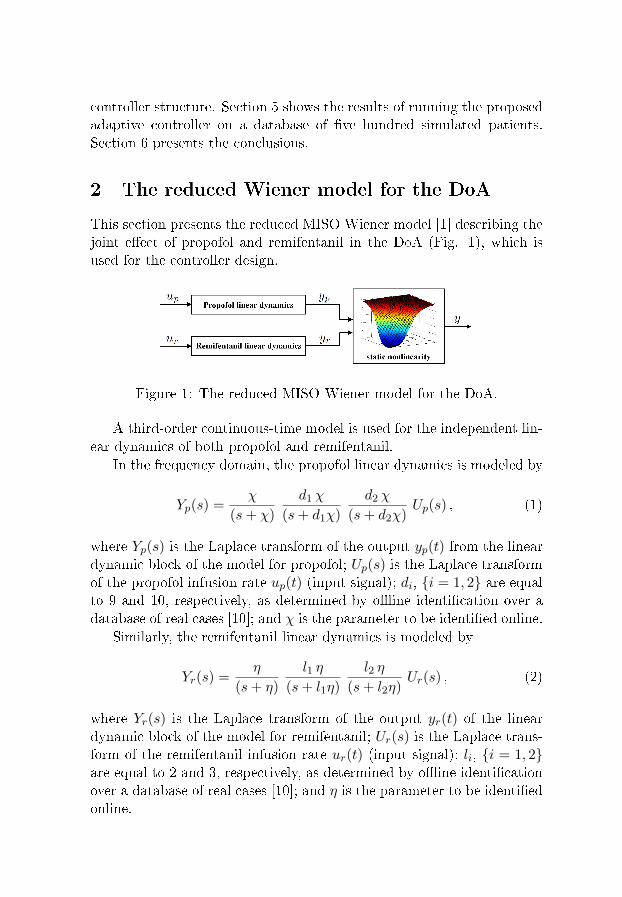
controller structure. Section 5 shows the results of running the proposedadaptive controller on a database of �ve hundred simulated patients.Section 6 presents the conclusions.

2 The reduced Wiener model for the DoA

This section presents the reduced MISO Wiener model [1] describing thejoint e�ect of propofol and remifentanil in the DoA (Fig. 1), which isused for the controller design.

Figure 1: The reduced MISO Wiener model for the DoA.

A third-order continuous-time model is used for the independent lin-ear dynamics of both propofol and remifentanil.

In the frequency domain, the propofol linear dynamics is modeled by

Yp(s) =χ

(s+ χ)

d1 χ

(s+ d1χ)

d2 χ

(s+ d2χ)Up(s) , (1)

where Yp(s) is the Laplace transform of the output yp(t) from the lineardynamic block of the model for propofol; Up(s) is the Laplace transformof the propofol infusion rate up(t) (input signal); di, {i = 1, 2} are equalto 9 and 10, respectively, as determined by o�ine identi�cation over adatabase of real cases [10]; and χ is the parameter to be identi�ed online.

Similarly, the remifentanil linear dynamics is modeled by

Yr(s) =η

(s+ η)

l1 η

(s+ l1η)

l2 η

(s+ l2η)Ur(s) , (2)

where Yr(s) is the Laplace transform of the output yr(t) of the lineardynamic block of the model for remifentanil; Ur(s) is the Laplace trans-form of the remifentanil infusion rate ur(t) (input signal); li, {i = 1, 2}are equal to 2 and 3, respectively, as determined by o�ine identi�cationover a database of real cases [10]; and η is the parameter to be identi�edonline.

The static nonlinearity is as follows [1]:

F : (c(t), ζ) ∈ [0,+∞[× ]0,+∞[ 7−→ y(t) = F(c(t), ζ) ∈ ]0, y0] ,

where

F(c(t), ζ) =y0

1 + (c(t))ζ, (3)

c(t) = myp(t)

C50p+yr(t)

C50r, (4)

and y(t) is the output of the MISO Wiener model; F is a static Hill func-tion; y0 is the baseline for the system output (zero drug e�ect); C50p andC50r are propofol and remifentanil normalizing constants, respectively,as determined by o�ine identi�cation over a database of real cases [10];and m and ζ are the parameters to be identi�ed in the nonlinearity.

The total number of patient-dependent parameters in the reducedmodel is hence four and the parameter vector becomes

θ = [χ η m ζ] T . (5)

3 The adaptive controller

3.1 Structure

The structure of the exactly linearizing adaptive controller proposed inthis paper is shown in Fig. 2. At each time step four main tasks aresequentially performed: identi�cation of the model parameters in thereduced MISO Wiener model by an extended Kalman �lter (EKF); ex-act linearization of the system using the current parameter estimates;estimation of the output of each linear block in the Wiener structureand of the linearized reference value by two Kalman �lters (KF); andcalculation of the control action by a linear quadratic gaussian (LQG)controller using the estimates of the parameters in the linear blocks ofthe Wiener model, after linearization [11, 12, 13].

3.2 Model parameters recursive identi�cation

At each time step the EKF block in Fig. 2 uses the measured BIS y andthe drug doses u to estimate the parameters in (5). For this, a state-spacerepresentation of the system has to be formulated in continuous-time,

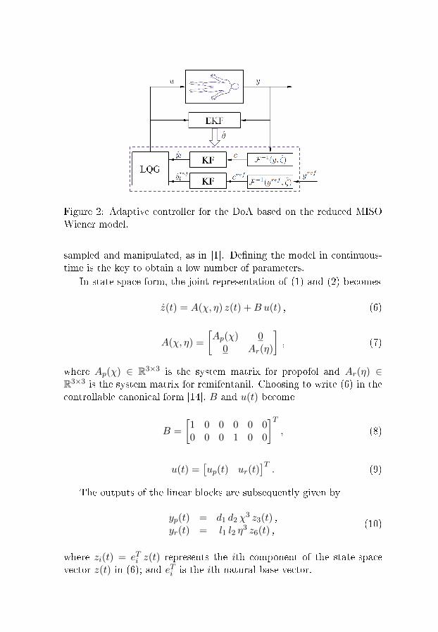
Figure 2: Adaptive controller for the DoA based on the reduced MISOWiener model.

sampled and manipulated, as in [1]. De�ning the model in continuous-time is the key to obtain a low number of parameters.

In state-space form, the joint representation of (1) and (2) becomes

z(t) = A(χ, η) z(t) +B u(t) , (6)

A(χ, η) =

[Ap(χ) 0

0 Ar(η)

], (7)

where Ap(χ) ∈ R3×3 is the system matrix for propofol and Ar(η) ∈R3×3 is the system matrix for remifentanil. Choosing to write (6) in thecontrollable canonical form [14], B and u(t) become

B =

[1 0 0 0 0 00 0 0 1 0 0

]T, (8)

u(t) =[up(t) ur(t)

]T. (9)

The outputs of the linear blocks are subsequently given by

yp(t) = d1 d2 χ3 z3(t) ,

yr(t) = l1 l2 η3 z6(t) ,

(10)

where zi(t) = eTi z(t) represents the ith component of the state-spacevector z(t) in (6); and eTi is the ith natural base vector.

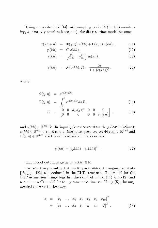
Using zero-order hold [14] with sampling period h (for BIS monitor-ing, h is usually equal to 5 seconds), the discrete-time model becomes

x(kh+ h) = Φ(χ, η)x(kh) + Γ(χ, η)u(kh) , (11)

yl(kh) = C x(kh) , (12)

c(kh) =[

mC50p

1C50r

]yl(kh) , (13)

y(kh) = F(c(kh), ζ) =y0

1 + (c(kh))ζ, (14)

where

Φ(χ, η) = eA(χ,η)h ,

Γ(χ, η) =

∫ h

0eA(χ,η)s dsB , (15)

C =

[0 0 d1 d2 χ

3 0 0 00 0 0 0 0 l1 l2 η

3

], (16)

and u(kh) ∈ R2×1 is the input (piecewise constant drug dose infusions);x(kh) ∈ R6×1 is the discrete-time state-space vector; Φ(χ, η) ∈ R6×6 andΓ(χ, η) ∈ R6×1 are the sampled system matrices; and

yl(kh) = [yp(kh) yr(kh)]T . (17)

The model output is given by y(kh) ∈ R.To recursively identify the model parameters, an augmented state

[15, pp. 422] is introduced in the EKF structure. The model for theEKF estimation brings together the sampled model (11) and (12) anda random walk model for the parameter estimates. Using (5), the aug-mented state vector becomes

x =[x1 . . . x6 x7 x8 x9 x10

]T=

[x1 . . . x6 χ η m ζ

]T , (18)

and the augmented state-space model becomes

x(kh+ h) =

[Φ(χ, η) 0

0 I

] [x(kh)θ(kh)

]+

+

[Γ(χ, η)

0

]u(kh) + w(kh)

≡

f1(kh, x(kh), u(kh))...

f10(kh, x(kh), u(kh))

+ w(kh)

≡ f(kh, x(kh), u(kh)) + w(kh) , (19)

y(kh) =y0

1 +(x9

d1 d2 x37 x3C50p

+l1 l2 x38 x6C50r

)x10 + e(kh)

≡ h(kh, x(kh)) + e(kh) , (20)

The time dependency of the augmented state vector componentsxi(kh), {i = 3, 6, 7, 8, 9, 10} in (20) was omitted due to space limitations.

As in [1], the linearization of f(kh, x(kh), u(kh)) and h(kh, x(kh))needed for the EKF (see [16, pp. 247]) was performed analytically.

3.3 Exact linearization

Both the measured BIS from the patient (output y) and the BIS referencevalue yref in Fig. 2 are �rst inverted through F−1 [11, 12, 13] usingthe current estimate of ζ given by the EKF identi�cation block. Thisprovides estimates for the mixture concentrations

c(kh) = F−1(y(kh), ζ) , and

cref (kh) = F−1(yref (kh), ζ) . (21)

It should be stressed that F(·, ·) is a bijective function and both y andyref in Fig. 2 lay within ]0, y0] as consequence of monitoring restrictionsof the BIS in the clinical practice. Moreover, as a result of a projectionalgorithm in the EKF structure [10], ζ is also lower-bounded. Due to this,and considering the domains a�ecting F(·, ·) (3), no problems arise in thisinversion. Ideally, when ζ is accurately estimated and no disturbances arepresent, F(·, ζ) is a perfect model of the static nonlinearity and the loop

becomes linear. However, the contribution of propofol and remifentanilto the mixture concentrations c and cref is still unknown. Consequently,yl and y

refl in (17) are estimated by the KF blocks to provide the inputs

for the linear controller. This means that the output of the linear blocksof the Wiener system appears directly as input for the linear controller.The LQG controller is therefore designed to control the outputs of thelinear dynamic part of the MISO Wiener type system as if there was nostatic nonlinearity.

Unlikely the SISO neuromuscular blockade case, to which an adap-tive controller was proposed in [13], the linear dynamics in the Wienermodel is MIMO in the DoA case, as shown in Fig. 1. Hence, a linearcontroller able to cope with that structure has to be chosen. Due to itsstructure, which enables the independent tuning of the contribution ofeach input to the cost function, a LQG controller was designed for theexactly linearized plant.

3.4 Linear quadratic gaussian controller design

After exact linearization of the Wiener model, an optimal regulator forthe system (11) and (12) can be designed. The feedback is given by

u(kh) = −L(kh) x(kh|kh− h) , (22)

where x(kh|kh− h) is the estimated state-space vector (11); and L(kh)is the solution of the discrete-time Ricatti equation [16].

The corresponding loss function is

l(x, u) = xT (Nh)Q0 x(Nh) + (23)

+

N−1∑n=0

[xT (nh) uT (nh)

] [Q1 Q12

Q21 Q2

] [x(nh)u(nh)

],

where the symmetric weighting matrices satisfy [16, pp. 319],

Q0 ≥ 0 , Q2 > 0 and[Q1 Q12

Q21 Q2

]≥ 0.

Furthermore, when the model states have to be estimated from dataand a reference signal (yrefl in this case) should be followed without anystatic error, an integral action is added to the control law (22). Thereason is as usual that the modeling errors need to be regulated away by

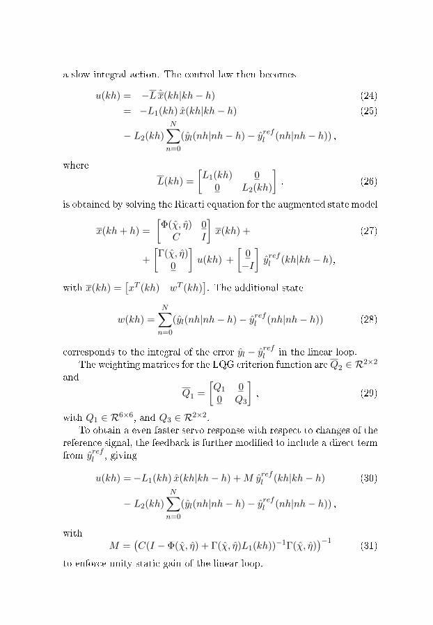
a slow integral action. The control law then becomes

u(kh) = −L x(kh|kh− h) (24)

= −L1(kh) x(kh|kh− h) (25)

− L2(kh)

N∑n=0

(yl(nh|nh− h)− yrefl (nh|nh− h)) ,

where

L(kh) =

[L1(kh) 0

0 L2(kh)

]. (26)

is obtained by solving the Ricatti equation for the augmented state model

x(kh+ h) =

[Φ(χ, η) 0C I

]x(kh) + (27)

+

[Γ(χ, η)

0

]u(kh) +

[0−I

]yrefl (kh|kh− h),

with x(kh) =[xT (kh) wT (kh)

]. The additional state

w(kh) =

N∑n=0

(yl(nh|nh− h)− yrefl (nh|nh− h)) (28)

corresponds to the integral of the error yl − yrefl in the linear loop.The weighting matrices for the LQG criterion function areQ2 ∈ R2×2

and

Q1 =

[Q1 00 Q3

], (29)

with Q1 ∈ R6×6, and Q3 ∈ R2×2.To obtain a even faster servo response with respect to changes of the

reference signal, the feedback is further modi�ed to include a direct termfrom yrefl , giving

u(kh) =−L1(kh) x(kh|kh− h) +M yrefl (kh|kh− h) (30)

− L2(kh)N∑n=0

(yl(nh|nh− h)− yrefl (nh|nh− h)) ,

withM =

(C(I − Φ(χ, η) + Γ(χ, η)L1(kh))−1Γ(χ, η)

)−1(31)

to enforce unity static gain of the linear loop.

4 Methods

4.1 Simulated system: Monte Carlo models

Previous studies on the reduced model [1] show that the minimal de-sign describes the input-output relationship between the administeredpropofol and remifentanil doses and the measured DoA in an accurateway. It should nevertheless be kept in mind that this minimal modelwas developed based on the standard physiology-based PK/PD model,mainly to overcome identi�ability issues due to the poor excitation prop-erties of the input signals. Hence, and in order to assess the performanceof the controller in conditions that are as realistic as possible, the realpatient in Fig. 2 was simulated using the standard PK/PD models forpropofol and remifentanil. A database of 500 cases was hence generatedconsidering the synergistic nonlinear interaction between propofol andremifentanil in the DoA (Table 1).

Table 1: Database of 500 simulated patients.

Propofol PK RemifentanilPK

PD interaction

125 femaleMarsh model [17] Minto model [5] log-normal distrib.

125 male125 female

Schnider model [4](mean & variances

125 male from [18])

Weight, height and age covariates needed to calculate the parametersin the PK models were randomly generated following a uniform distri-bution, considering weight ∈ [60, 80] kg, height ∈ [160, 180] cm, and age∈ [18, 70] years.

4.2 User choices

The BIS target after induction was set inside [40,60], as recommendedby the BIS monitor manufacturer for general anesthesia cases.

Taking into account the magnitude of the propofol and remifentanilinfusion rates administered in the clinical practice, the LQG diagonal

weighting matrices were chosen as

Q1 = diag ([1 0.1 0.01 10 1 0.1]) ,

Q2 = diag ([0.1 100]) ,

Q3 = diag ([0.0001 0.1]) ,

5 Results and discussion

This section presents simulation results on the performance of the pro-posed exactly linearizing adaptive controller for the DoA, using BIS mea-surements.

Figure 3 shows the results that were obtained when the PK param-eters from a 50 years old, 170 cm height and 70 kg male patient wereused to simulate the propofol and remifentanil PK. For the nonlineardrugs interaction, the mean parameters in [18] were used. Zero-meannoise with variance 2 was added to the output y. After induction, theBIS reference is a square wave of amplitude 2.5 around the setpoint of50.

As it is clear in Fig. 3(a) the BIS output y follows the referencepro�le with no static error. This is the result from the integral actionthat was added to the standard LQG formulation. This good trackingperformance is a consequence of the use of the online parameter estimatesin Fig. 3(b) that are provided by the EKF. The administered propofoland remifentanil doses enabling such tracking behavior are shown in Fig.3(c).

In order to numerically evaluate the robustness of the controller withrespect to inter and intrapatient variability, the same adaptive structurewas applied to all 500 Monte Carlo models in the database. After induc-tion, the BIS reference was set constant on a value of 50 and zero meannoise with variance 2 was added as measurement noise. Results for 487cases are shown in Fig. 4. The remaining 13 cases, with a median abso-lute performance error (MAPE) greater than 10%, were excluded fromthe analysis. The mean values for the controlled BIS, parameter esti-mates, and propofol and remifentanil calculated rates for the 487 casesare shown in solid line in Fig. 4. The mean plus, and minus standarddeviations are plotted in dashed and dotted lines, respectively.

Fig. 4(a) clearly shows that the controlled BIS is regulated to thetarget level of 50. The small di�erence between the mean, the mean plusand the mean minus the standard deviation indicates that this behavior

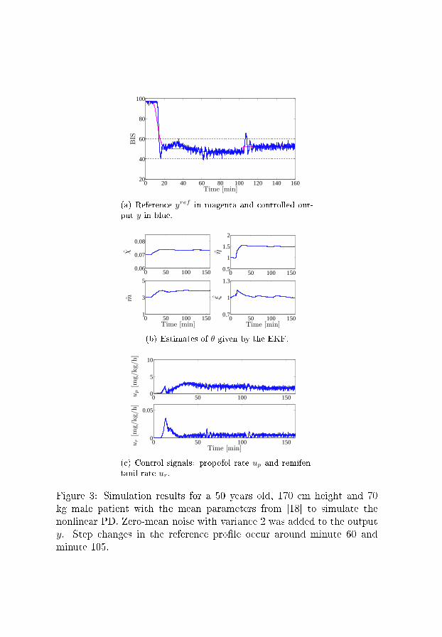
0 20 40 60 80 100 120 140 16020

40

60

80

100

BIS

Time [min]

(a) Reference yref in magenta and controlled out-put y in blue.

0 50 100 1500.06

0.07

0.08

χ

0 50 100 1500.5

1

1.5

2

η

0 50 100 1501

3

5

Time [min]

m

0 50 100 1500.7

1

1.3

Time [min]

ξ

(b) Estimates of θ given by the EKF.

0 50 100 1500

5

10

up[m

g/kg/h]

0 50 100 1500

0.05

Time [min]

ur[m

g/kg/h]

(c) Control signals: propofol rate up and remifen-tanil rate ur.

Figure 3: Simulation results for a 50 years old, 170 cm height and 70kg male patient with the mean parameters from [18] to simulate thenonlinear PD. Zero-mean noise with variance 2 was added to the outputy. Step changes in the reference pro�le occur around minute 60 andminute 105.

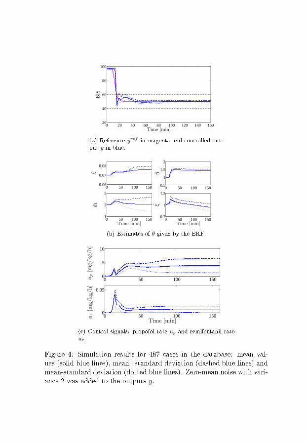
0 20 40 60 80 100 120 140 16020

40

60

80

100

BIS

Time [min]

(a) Reference yref in magenta and controlled out-put y in blue.

0 50 100 1500.06

0.07

0.08

χ

0 50 100 1500.5

1

1.5

2η

0 50 100 1501

3

5

Time [min]

m

0 50 100 1500.7

1

1.3

Time [min]

ξ

(b) Estimates of θ given by the EKF.

0 50 100 1500

5

10

up[m

g/kg/h]

0 50 100 1500

0.05

Time [min]

ur[m

g/kg/h]

(c) Control signals: propofol rate up and remifentanil rateur.

Figure 4: Simulation results for 487 cases in the database: mean val-ues (solid blue lines), mean+standard deviation (dashed blue lines) andmean-standard deviation (dotted blue lines). Zero-mean noise with vari-ance 2 was added to the outputs y.

is consistent in all 487 simulated cases. The estimated parameters areshown in Fig. 4(b). Aiming for a short induction time, the initial co-variance matrices related to the parameter estimates were chosen to behigh, which resulted in a fast update of the parameter estimates duringthe initial minutes.

Using the mean and standard deviations obtained from these simula-tions, the coe�cient of variation (cv) of the parameters can be obtained:cvχ = 4.49%, cvη = 6.99%, cvm = 39.2%, and cvξ = 10.3%. The factthat the coe�cients of variation for the estimated parameters are highis a further motivation for the use of the EKF to recursively identify themodel parameters in the controller structure.

Fig. 4(c) shows the calculated control inputs (propofol and reminfen-tanil rates). These values are in accordance with the dosage guidelinesfor maintenance of general anesthesia when a combination of propofoland remifentanil is intravenously administrated. For propofol, the rec-ommended dosage for adult patients (less than 55 years of age) is 6 to 12mg/kg/h; for elderly, debilitated and/or adult ASA III or IV patients,it is 3 to 6 mg/kg/h [19]. These values should reduce by up to 75%when propofol is administered together with remifentanil. At time 160,up = 3.89 mg/kg/h and σp = 2.61 mg/kg/h. For remifentanil, when usedwith propofol, the recommended maintenance dosage ranges from 0.003to 0.12 mg/kg/h [20]. At time 160, ur = 0.006 mg/kg/h and σr = 0.006mg/kg/h.

6 Conclusions

This paper presented an exactly linearizing adaptive controller for propo-fol and remifentanil administration in general anesthesia cases. The con-trolled output is the depth of anesthesia bispectral index (BIS). For thecontroller design, a reduced MISO Wiener model [1] is used, being itscontinuous-time parameters estimated online by an extended Kalman�lter (EKF). By using the nonlinear parameter estimates, the Wienermodel is exactly linearized at each time step and a linear quadratic gaus-sian (LQG) controller using the parameter estimates from the linear partof the Wiener model was designed to control the linearized plant.

With this setup, the main drawback of identifying and controlling anoverparameterized under-excited model is no more present, as it wouldbe if the standard models describing the pharmacokinetics and phar-macodynamics of propofol and remifentanil were used for the controller

design.The performance and robustness of the controller was assessed by

running Monte Carlo simulations on a database of 500 models. Goodtracking results were obtained on 97% of the cases. In order to reducethe remaining 3% of cases where the controlled BIS lied outside theadmissible range of [40,60], additional safety nets and constraints on theestimates are needed. This stands as future work for this research line.

Stability and convergence properties of the controller is also a topicfor further research.

Acknowledgments

The research leading to these results received funding from Fundaçãopara a Ciência e a Tecnologia via the project Galeno PTDC/SAU-BEB/103667/2008, and from the European Research Council via the AdvancedGrant 247035.

References

[1] M. M. Silva, T. Mendonça, and T. Wigren, �Online nonlinear iden-ti�cation of the e�ect of drugs in anaesthesia using a minimal pa-rameterization and BIS measurements,� in Proc. American Control

Conference (ACC'10), jun 30-jul 2 2010.

[2] T. J. Gan, P. S. Glass, A. Windsor, F. Payne, C. Rosow, P. Sebel,and P. Manberg, �Bispectral index monitoring allows faster emer-gence and improved recovery from propofol, alfentanil, and nitrousoxide anesthesia,� Anesthesiology, vol. 87, 1997.

[3] T. Wigren, �Recursive prediction error identi�cation method usingthe nonlinear Wiener model,� Automatica, vol. 29(4), pp. 1011�25,1993.

[4] T. W. Schnider, C. F. Minto, P. L. Gambus, C. Andresen, D. B.Goodale, S. L. Shafer, and E. J. Youngs, �The in�uence of method of

administration and covariates on the pharmacokinetics of propofolin adult volunteers,� Anesthesiology, vol. 8, no. 5, pp. 1170�82, 1998.

[5] C. F. Minto, T. W. Schnider, T. D. Egan, E. Youngs, H. J. Lem-mens, P. L. Gambus, V. Billard, J. F. Hoke, K. H. Moore, D. J.Hermann, K. T. Muir, J. W. Mandema, and S. L. Shafer, �In�uenceof age and gender on the pharmacokinetics and pharmacodynamicsof remifentanil. I. Model development,� Anesthesiology, vol. 86, pp.10�23, 1997.

[6] J.-O. Hahn, G. A. Dumont, and J. M. Ansermino, �Closed-loop anes-thetic drug concentration estimation using clinical-e�ect feedback,�IEEE Trans Biom Eng, vol. 58, no. 1, pp. 3�6, jan. 2011.

[7] A. R. Absalom and M. M. R. F. Struys, Overview of Target Con-

trolled Infusions and Total Intravenous Anaesthesia, 2nd ed. Gent:Academia Press, 2007.

[8] M. M. R. F. Struys, T. D. Smet, L. F. M. Versichelen, S. V. de Velde,R. V. den Broecke, and E. P. Mortier, �Comparison of closed-loopcontrolled administration of propofol using bispectral index as thecontrolled variable versus 'standard practice' controlled administra-tion,� Anesthesiology, vol. 95, no. 1, pp. 6�17, jul 2001.

[9] N. Liu, T. Chazot, S. Hamada, A. Landais, N. Boichut, C. Dussaus-soy, B. Trillat, L. Beydon, E. Samain, D. I. Sessler, and M. Fischler,�Closed-loop coadministration of propofol and remifentanil guidedby bispectral index: A randomized multicenter study,� Anesthesia

and Analgesia, vol. 112, no. 3, pp. 546�57, mar 2011.

[10] M. M. Silva, T. Wigren, and T. Mendonça, �Nonlinear iden-ti�cation of the human response to anaesthesia by the useof BIS measurements,� Dept. Information Technology, UppsalaUniversity, Uppsala, Sweden, Tech. Rep. 2010-008, Available:http://www.it.uu.se/research/publications/reports/, Mar. 2010.

[11] K. J. Åström and B. Wittenmark, Adaptive Control, 2nd ed. Mi-neola, New York, USA: Dover Publications, Inc., 2008.

[12] T. Wigren and L. Brus, �Reduction of amplitude dependent gainvariations in control of non-linear Wiener type systems,� in Proc.

7th IFAC Symposium on Nonlinear Control Systems (NOLCOS'07),aug 22-24 2007, pp. 978�83.

[13] M. M. Silva, T. Mendonça, and T. Wigren, �Nonlinear adaptive con-trol of the neuromuscular blockade in anesthesia,� in Proc. IEEE

Conference on Decision and Control and European Control Confer-

ence (CDC-ECC'11), dec 11-15 2011, pp. 41�6.

[14] K. J. Åström and B. Wittenmark, Computer-Controlled Systems.Englewood Cli�s, NJ: Prentice Hall, 1984.

[15] L. Ljung and T. Söderström, Theory and Practice of Recursive Iden-ti�cation. Cambridge, Massachusetts: The MIT Press, 1983.

[16] T. Söderström, Discrete-time Stochastic Systems, 2nd ed. London,UK: Springer-Verlag, 2002.

[17] B. Marsh, M. White, N. Norton, and G. N. Kenny, �Pharmacokineticmodel driven infusion of propofol in children,� Br. J. Anaesthesia,vol. 67, pp. 41�8, 1991.

[18] M. J. Mertens, E. Olofsen, F. H. M. Engbers, A. G. L. Burm, J. G.Bovil, and J. Vuyk, �Propofol reduces perioperative remifentanilrequirements in a synergistic manner,� Anesthesiology, vol. 99, pp.347�59, 2003.

[19] AstraZeneca, Diprivan: Product monograph. AstraZeneca CanadaInc., april 2011.

[20] GlaxoSmithKline, Remifentanil (Ultiva): Summary of Product

Characteristics. GlaxoSmithKline UK, electronic Medicines Com-pendium, jan 2011.

Recent licentiate theses from the Department of Information Technology

2012-006 Martin Tillenius: Leveraging Multicore Processors for Scientific Computing

2012-005 Egi Hidayat: On Identification of Endocrine Systems

2012-004 Soma Tayamon: Nonlinear System Identification with Applications to SelectiveCatalytic Reduction Systems

2012-003 Magnus Gustafsson: Towards an Adaptive Solver for High-Dimensional PDEProblems on Clusters of Multicore Processors

2012-002 Fredrik Bjurefors: Measurements in Opportunistic Networks

2012-001 Gunnika Isaksson-Lutteman: Future Train Traffic Control – Development anddeployment of new principles and systems in train traffic control

2011-006 Anette Löfström: Intranet Use as a Leadership Strategy

2011-005 Elena Sundkvist: A High-Order Accurate, Collocated Boundary ElementMethod for Wave Propagation in Layered Media

2011-004 Niclas Finne: Towards Adaptive Sensor Networks

2011-003 Rebecka Janols: Tailor the System or Tailor the User? How to Make BetterUse of Electronic Patient Record Systems

2011-002 Xin He: Robust Preconditioning Methods for Algebraic Problems, Arising inMulti-Phase Flow Models

2011-001 David Eklöv: Efficient Methods for Application Performance Analysis

Department of Information Technology, Uppsala University, Sweden