System Identification and Control of an AerobotDrive System

Paul Pounds 1, Robert Mahony 2, Peter Corke 3

12Department of Engineering, Australian National UniversityBld 32 North Road, Acton ACT 0200 Australia,

paul.pounds@anu.edu.au, robert.mahony@anu.edu.au3ICT Robotics, CSIRO

1 Technology Court, Pullenvale QLD 4069 Australia, peter.corke@csiro.au

Abstract

Fast thrust changes are important for authoritive controlof VTOL micro air vehicles. Fixed-pitch rotors that alterthrust by varying rotor speed require high-bandwidth con-trol systems to provide adequate performace. We develop afeedback compensator for a brushless hobby motor driving acustom rotor suitable for UAVs. The system plant is identifiedusing step excitation experiments. The aerodynamic operatingconditions of these rotors are unusual and so experimentsare performed to characterise expected load disturbances. Theplant and load models lead to a proportional controller designcapable of significantly decreasing rise-time and propagationof disturbances, subject to bus voltage constraints.

1. INTRODUCTION

Dynamic control is critical to unmanned aerial vehicle (UAV)

flight. Craft that rely on changing rotor thrusts for manoeuver-

ing, such as small tandems, quad-rotors or blimps, are a subset

of UAVs for which rotor speed control is of great interest.

These micro air vehicles use fixed-pitch rotors that vary thrust

by changing angular velocity. Such designs avoid the complex

swashplate mechanisms of fully articuled blades and so offer

savings in complexity and maintenance. The robust simplicity

of this style of rotor is one of the key driving motivations for

the development of quad-rotor UAVs.

Fast response of the drive system is essential for attitude

control of UAVs equipped with fixed-pitch rotors. These drive

units must either have low rotor mass or use a control sys-

tem to artificially improve performance. The popular RCtoys

Draganflyer toy [2] uses light, simple rotors; most current

quad-rotors use RCtoys components. The Draganflyer does

not directly sense or control the rotor speed, but rather closes

the loop around the motors and attitude via pitch and roll

rate feedback. Larger quad-rotor UAVs, such as the Australian

National University’s (ANU) X-4 Flyer [8], have rotors with

much more inertia than Draganflyer rotors. These need some

schema to improve the bandwidth of the rotor response for

attitude control to be robust.

Small-scale rotors in quad-rotor craft present a set of

aerodynamic conditions that are unusual among aircraft. Iden-

Fig. 1: Complete VTOL Thruster.

tifying likely disturbances resulting from the operation of the

rotors allows for the frequency response of the closed loop

system to be tuned to reject unwanted variations in rotor speed.

Transient environmental influences, such as gusts or wash from

obstacles, are likely to be encountered by quad-rotor aircraft

designed to operate in indoor spaces. Elimination of rotor

speed deviations is desirable as this reduces the propagation

of disturbances into the attitude dynamics of the vehicle. As

yet, the influence of in-flight disturbances on small-scale rotor

speed has not yet been explored.

The controller for the small scale rotor drives we have

developed (cf. Fig. 1) must improve the system bandwidth

sufficiently for authorative attitude control on a quad-rotor

vehicle. Rather than rely on empirial tuning or more complex

nonlinear treatments, a rigorously designed controller based on

a combined system model of the plant, verified by experiment,

is warranted.

The compensator must be well-conditioned when used with

a craft of loosely known and often changing flight parameters.

The design must not exceed the limitations of the hardware in

which it is implemented. Non-linearities of the system present

bounds on the controller performance that must be respected.

The controller is intentionally simple and practical to improve

154

2007 Information, Decision and Control

1-4244-0902-0/07/$20.00 2007 IEEE

the reliability of the system.

There are well developed theories for the control of fan

speed driven by electric motors. Cogdel [1] and Innovatia [5]

give comprehensive overviews of the dynamics of brushless

motors, and Franklin and Powell [3] provide examples of

motor control. Although more complex control methods exist,

they are not appropriate technology to a system motivated by

simplicity.

This paper is a case-study in the development of feedback

control compensator for regulating rotor speed and improving

bandwidth of an integrated drive control system for a small

vertical take-off and landing (VTOL) aircraft. We outline the

performance specifications of a custom rotor, motor and power

system. We test the rotors for dynamic response and identify

a model of the system plant and disturbances. We describe

the process used to develop performance requirements and the

logic behind the compensator design. Finally, we present the

measured performance of the implemented controller.

2. HARDWARE

Each drive system consists of four components: rotors, motors,

control boards and batteries, described below.

• Rotor

The rotor is superficially similar to hobby aeroplane

propellers. Unlike airscrews, the rotors must be matched

to static thrust conditions. This makes the rotor blades

thin and flexible with a flapping hinge, rather than chunky

with high pitch angles [9].

• Motor

Jeti Phasor 30-3 three-phase brushless motors for radio-

controlled aircraft were selected for their high torque

performance that allows for direct drive of the rotors,

eliminating the need for gearing. The motors can pass

more than 300 W and are rated up to 35 A.

• Controller Board

Brushless motors require electronic commutation. RC

hobby controllers are unsuitable due to non-linearities

and bandwidth limitations. Custom control boards were

made by the CSIRO ICT Queensland Centre for Ad-

vanced Technology group, based around the Freescale

HC12D60A microprocessor and Toshiba TB9060 brush-

less motor speed controller .

The boards also include an integrator single-phase back-

emf speed sensor, as well as voltage and current sensors.

The resolution of the speed sensor is limited by the

rotation rate of the rotor and the number of magnetic

poles. The maximum speed measurement refresh rate

is 400 Hz and the current and voltage refresh rates are

50 Hz.

• Power

Power is supplied by 32 Kokam lithium ion 1500 mAh

high-discharge cells. Each cell has a nominal voltage of

3.7 V, ranging from 4.2 V fully charged and dropping to

3 V at depletion. Each cell can deliver 12 A constantly,

or 15 A for short bursts. The batteries are connected in

two parallel sets of four cells in series; that is, 14.8 V

nominal voltage and 24 A of current.

3. ROTOR PERFORMANCE

Momentum theory provides a relationship between thrust,

induced velocity and power in the rotor [10, pp6-7]. Using

energy conservation, it can be shown that in hover:

Pi =T

32√

2ρA(1)

where T is the thrust produced, ρ is air density, A is the area

of the rotor disc and Pi is the power induced in the air.

The Figure of Merit (F.M .) of the rotor is the ratio of power

induced in the air and power in the rotor shaft:

F.M. =Pi

Ps(2)

This is used to model rotor efficiency when calculating the

theoretical onboard power requirements.

For a quad-rotor helicopter weighing 4 kg with a 30 per cent

control margin, each motor must produce 12.7 N of thrust.

The rotor radius is limited to less than 0.165 m, due to the

size of the robot, leading to a requirement of 101.2 W of

power induced in the air. The rotational velocity was set to

800 rads−1. The lithium ion cells have a current limit of

22 A, producing a maximum 0.1749 Nm motor torque. This

gives the drive a top shaft power of 131 W. The maximum

theoretical thrust is 15.1 N per motor (assuming F.M. = 1).

The actual rotor design F.M. must be no less than 0.77.

In practice, the blades created were capable of producing

14.3 N at approximately 1000 rads−1, a F.M. of 0.71, but

with a higher rotor speed.

4. DYNAMIC MODEL IDENTIFICATION

Fast dynamic response of rotor speed is essential for ef-

fective performance. Controlling the motors via a feedback

compensator is a simple way to extract better rise-time. To

design a controller, an accurate characterisation of the system

is necessary. This is found using a set of step response

experiments to identify the open loop plant of X-4’s motor-

rotor system previously described.

A. Dynamic Model Structure and Nonlinearities

The dynamic model of the rotor-motor system is composed

of a cascade of the rotor aerodynamics, motor dynamics and

battery response.

• Rotor Aerodynamics

The rotor torque is modelled as a constant gain at

operating conditions. The step response of the rotors

is also expected to be very fast. Leishmann provides a

quantitative estimate of the timescale of unsteady flow [6,

pp369-371]. We found the flow rise-time of these rotors

to be of the order of one blade revolution (less than 8 ms).

This is very fast compared to the plant mechanics and so

is not included in the model.

155

• Motor Poles

From Cogdell [1, p805], the dynamics of an ideal brush-

less motor system is given to be a two-pole system.

One pole is associated with the rigid body dynamics of

the motor and the other with the electrical dynamics of

the windings. The mechanical pole is governed by the

rotational inertia of the drive – the combined total of

the rotating motor armature, blades, hub and mast. The

electrical dynamic of brushless motors is typically very

fast and is omitted.

• Battery Model

Based on the theory and example cell parameters given

in Gao et al [4], the flyer batteries are expected to

have a one-pole, one-zero system model. No explicit

identification of the battery dynamics has been performed.

From previous experiments, it is known that the cells

do not have a constant voltage during discharge. The

voltage per cell drops substantially during the first and

last 100 mAh of discharge. The mid-zone of operation is

a gently decreasing slope. The rate of the battery voltage

change is slow and we do not believe it will substantially

affect the dynamics of the system.

The total cascaded system model is expected to take the

form of two poles and one zero:

H =k(s + zb)

(s + pm)(s + pb)(3)

Where H is the plant model, k is the rotor gain, zb is the

battery zero and pm and pb are the motor and battery poles.

B. Step Response Experiments

The thruster step response was found using input excitation

experiments. The data are used to identify the model param-

eters, based on the expected model stucture.

The step signal is a Pulse Width Modulated (PWM) signal

sent to the motor control chip in a 255-step duty cycle, to

modulate the pulse widths of voltage sent to the motor drive

phases and drive the rotor. The drive components are mounted

on the X-4 Flyer for the test. The flyer is fastened to a testbed

that holds the robot off the ground and allows it to be locked

in place or pivoted freely along the pitch axis.

The helicopter will predominately operate around hover,

with a rotor speed of 850 rads−1. The reference signals

of 175-225 PWM units produce speeds of 820-920 rads−1,

respectively. This is a step across the full expected range of

the rotor. The ID experiment was performed with a train of

70 step inputs, each with a period of 6 seconds.

A National Instruments 6024E DSP card captured the rotor’s

speed and input reference signal via a filtered frequency-

to-voltage converter reading from one of the motor’s three

phases. The onboard speed measurement capabilities of the

motor controller boards were not used for the identification as

the data output of the sensor boards is limited to 50 Hz and

is unsuitable for this purpose. The DSP measures a voltage

produced by a speed sensor that reads the back-emf frequency

of one of the motor phases. The sensor board has dynamics

Fig. 2: Averaged Step Response Data of FH and Identified Model

associated with low-pass filters and a charge pump with slow

electrical dynamics. The sensor board transfer function is:

F =442

(s + 45)(s + 9.7)(4)

The DSP samples at 1 kHz and the speed sensor can resolve

speed differences of 1.2 rads−1.

All of the tests were averaged to increase the signal-to-noise

ratio (SNR) of the data. The noise of the signal has a peak-to-

peak magnitude of 10 rads−1, for an SNR of 38 dB. Averaging

the step responses increases the SNR to 57 dB. The model

identified included a 0.02 second time delay in the system;

this is attributed to the influence of fast dynamic effects and

processor transport delay. The averaged measured response

curve data of the combined plant and sensor dynamics, with

the estimated sensor-plant model step response super-imposed,

is shown in (cf. Fig. 2).

The plant transfer function is found by inverting the iden-

tified combined sensor-thruster system by the known sensor

model. The identified thruster response was found to be:

H =23(s + 0.43)

(s + 9.6)(s + 0.54)(5)

The pole-zero pair is attributed to the slow dynamics of the

batteries, and one dominant pole to the mechanical response of

the rotor. Although filtering the logged data with an inverted

sensor model produced a noisy signal, the output had good

agreement with the expected drive dynamics.

The step response and Bode plot of the plant appear in

figures (cf. Fig. 3) and (cf. Fig. 4).

Associated with the lithium ion cells is a slew rate non-

linearity. When the motor is given a large step instruction, the

instantaneous current flow is large – in the order of 100 A.

The internal resistance of the cells causes the terminal voltage

of the battery to fall dramatically during high current draw.

The motor control board is powered by a 5 V regulator across

the input supply – if the battery voltage falls below this,

the microprocessor loses power and resets. For this reason,

156

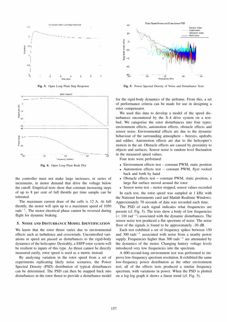
Fig. 3: Open Loop Plant Step Response

Fig. 4: Open Loop Plant Bode Plot

the controller must not make large increases, or series of

increments, in motor demand that drive the voltage below

the cutoff. Empirical tests show that constant increasing steps

of up to 8 per cent of full throttle per time sample can be

tolerated.

The maximum current draw of the cells is 12 A. At full

throttle, the motor will spin up to a maximum speed of 1050

rads−1. The motor electrical phase cannot be reversed during

flight for dynamic braking.

5. NOISE AND DISTURBANCE MODEL IDENTIFICATION

We know that the rotor thrust varies due to environmental

effects such as turbulence and crosswinds. Uncontrolled vari-

ations in speed are passed as disturbances to the rigid-body

dynamics of the helicopter. Desirably, a SSFP rotor system will

be resilient to inputs of this type. As thrust cannot be directly

measured easily, rotor speed is used as a metric instead.

By analysing variation in the rotor speed from a set of

experiments replicating likely noise scenarios, the Power

Spectral Density (PSD) distribution of typical disturbances

can be determined. The PSD can then be mapped back into

disturbances in the rotor thrust to provide a disturbance model

Fig. 5: Power Spectral Density of Noise and Disturbance Tests

for the rigid-body dynamics of the airframe. From this, a set

of performance criteria can be made for use in designing a

rotor compensator.

We used this data to develop a model of the speed dis-

turbances encountered by the X-4 drive system on a test-

bed. We catagorise the rotor disturbances into four types:

environment effects, automotion effects, obstacle effects and

sensor noise. Environmental effects are due to the dynamic

behaviour of the surrounding atmosphere – breezes, updrafts

and eddies. Automotion effects are due to the helicopter’s

motion in the air. Obstacle effects are caused by proximity to

objects and surfaces. Sensor noise is random level fluctuation

in the measured speed values.

Four tests were performed:

• Environment effects test – constant PWM, static position

• Automotion effects test – constant PWM, flyer rocked

back and forth by hand

• Obstacle effects test – constant PWM, static position, a

large flat surface moved around the rotor

• Sensor noise test – motor stopped, sensor values recorded

In each test, the rotor speed was sampled at 1 kHz with

the National Instruments card and Matlab Realtime Windows.

Approximately 70 seconds of data was recorded each time.

The PSD of each signal indicates what frequencies are

present (cf. Fig. 5). The tests show a body of low frequencies

(< 100 rad−1) associated with the dynamic disturbances. The

sensor noise test produced a flat spectrum of noise. The noise

floor of the signals is found to be approximately -30 dB.

Each test exhibited a set of frequency spikes between 150

and 300 rads−1 associated with noise from a nearby power

supply. Frequencies higher than 300 rads−1 are attenuated by

the dynamics of the motor. Changing battery voltage levels

introduced very low frequencies into the spectrum.

A 600-second-long environment test was performed to im-

prove low-frequency spectrum resolution. It exhibited the same

low-frequency power distribution as the other environment

test; all of the effects tests produced a similar frequency

spectrum, with variations in power. When the PSD is plotted

on a log-log graph it shows a linear trend (cf. Fig. 5).

157

It is interesting to note that the undisturbed test has the

greatest levels of higher-frequency noise. It is thought that

this is due to circulating currents and eddies building up

over time in a sustained flow. If the flow conditions are

constantly disturbed, such systems cannot manifest. As a

consequence, stable hover conditions correspond to the worse

noise characteristics for the system.

6. CONTROL

The rotor speed controller must primarily provide stable and

robust performance and disturbance rejection, as well as satisfy

the constraints of the system limitations. Foremost is the slew

rate; the controller implemention cannot exceed the slew rate

bound imposed to avoid critical voltage drops. Disturbance

rejection is also considered, as well as high frequency noise

and the effect of limit-cycles.

A. Requirements and Constraints

The rate limitation of the system sets an upper bound on the

gain and frequency of the input to the plant.

A maximum constraint for the realisable frequency response

of the system can be can be developed by considering the

fastest sinewave that the rate limitation can support. The

highest frequency that can be passed through the rate

saturation can be determined by equating the ramp magnitude

to the maximum slope of the sinewave at a given frequency.

The constraint is given as Ratelimit = B units/s.

For a sinewave:

u = A sin(ωt) (6)

du

dt= Aω cos(ωt) (7)

where A is the amplitude of the sinewave, t is time and uis the system input. The maximum slope is at cos(ωt) = 1:

Aω ≤ B (8)

Thus, A can be replaced with the magnitude of the input to

the motor system. The largest step passed to the system will

occur when the error is at the greatest expected value, Δe.

In the closed loop case, with controller C and plant H , the

bound (eq. 10) is derived as follows:

Δe‖C‖ω ≤ B (9)

‖C‖‖H‖ω ≤ B‖H‖Δe

(10)

20 log(‖C‖‖H‖) + 20 log(ω) ≤ 20 log(B‖H‖

Δe) (11)

20 log(‖C‖‖H‖) ≤ 20 log(B

Δe) (12)

+20 log(‖H‖) − 20 log(ω)

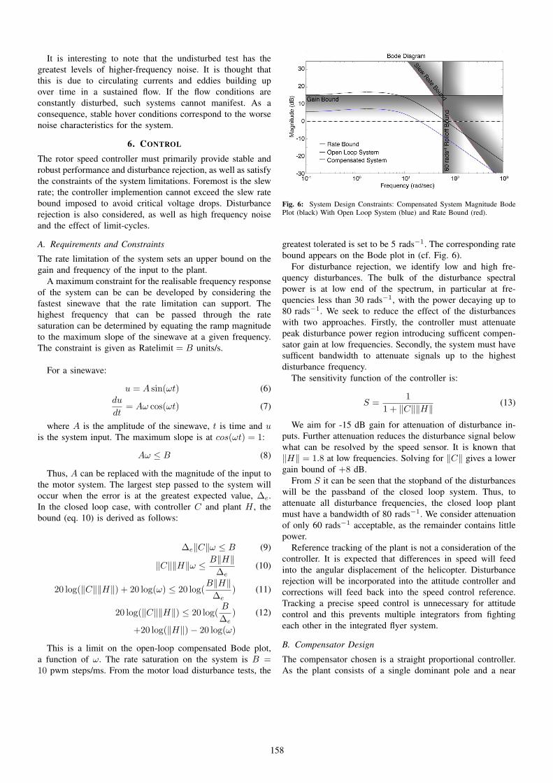
This is a limit on the open-loop compensated Bode plot,

a function of ω. The rate saturation on the system is B =10 pwm steps/ms. From the motor load disturbance tests, the

Fig. 6: System Design Constraints: Compensated System Magnitude BodePlot (black) With Open Loop System (blue) and Rate Bound (red).

greatest tolerated is set to be 5 rads−1. The corresponding rate

bound appears on the Bode plot in (cf. Fig. 6).

For disturbance rejection, we identify low and high fre-

quency disturbances. The bulk of the disturbance spectral

power is at low end of the spectrum, in particular at fre-

quencies less than 30 rads−1, with the power decaying up to

80 rads−1. We seek to reduce the effect of the disturbances

with two approaches. Firstly, the controller must attenuate

peak disturbance power region introducing sufficent compen-

sator gain at low frequencies. Secondly, the system must have

sufficent bandwidth to attenuate signals up to the highest

disturbance frequency.

The sensitivity function of the controller is:

S =1

1 + ‖C‖‖H‖ (13)

We aim for -15 dB gain for attenuation of disturbance in-

puts. Further attenuation reduces the disturbance signal below

what can be resolved by the speed sensor. It is known that

‖H‖ = 1.8 at low frequencies. Solving for ‖C‖ gives a lower

gain bound of +8 dB.

From S it can be seen that the stopband of the disturbances

will be the passband of the closed loop system. Thus, to

attenuate all disturbance frequencies, the closed loop plant

must have a bandwidth of 80 rads−1. We consider attenuation

of only 60 rads−1 acceptable, as the remainder contains little

power.

Reference tracking of the plant is not a consideration of the

controller. It is expected that differences in speed will feed

into the angular displacement of the helicopter. Disturbance

rejection will be incorporated into the attitude controller and

corrections will feed back into the speed control reference.

Tracking a precise speed control is unnecessary for attitude

control and this prevents multiple integrators from fighting

each other in the integrated flyer system.

B. Compensator Design

The compensator chosen is a straight proportional controller.

As the plant consists of a single dominant pole and a near

158

pole-zero cancellation, the plant cannot be sent unstable by the

application of gain. However, especially large values (K > 5)

will introduce limit-cycles in the plant, caused by saturating

the amplitude and slew rate bounds of the controller. We

choose a value of 3, such that the response is made as fast as

possible within the specified bounds.

From the model of the plant and non-linearities, we coded a

simulation of the rotor dynamics in Matlab Simulink. This was

used to assess the proportional controller and ensure that the

controller design did not produce limit-cycles oscillations. The

maximum step of 820–920 rads−1 may just begin to saturate

the actuator. As the rate limitation sets a maximum response

speed, this will ensure that the rise time is minimised without

pushing the motor beyond what the limitation allows for.

The gain selected slightly pushes the controller frequency

response out of the rate limitation bound at 5 rads−1. The

effect is not very pronounced and, given the improvements

in rise-time, is considered acceptable. From calculation, the

minimum gain necessary to satisfy the low frequency distur-

bance rejection criterion is 2.57. The system gain satisfies the

original -15 dB specification, reaching -16.12 dB.

The computed transfer function of the closed loop system

is:

Hcl =68.85(s + 0.42)

(s + 78.54)(s + 0.43)(14)

C. Performance

The control design was implemented on the CSIRO boards

and tested in the X-4 thrust test rig. The control loop runs

at 1 kHz on the microprocessor – a speed dictated by the

need to smoothly generate the rate-limited ramp output of

the controllers. All control computations were performed

with signed long variables, with up to 20-bits computational

precision available from the HC12 arithmetic logic unit.

We repeated the ID process for the closed loop plant to

confirm that the controller performs as designed. The identi-

fication showed good agreement with the calculated system:

Hcl =83(s + 0.0046)

(s + 99)(s + 0.0042)(15)

The implemented system has a rise-time of 0.05 seconds

and no overshoot. Higher gains were tested on the controller,

but we felt the resulting cyclic behaviour that developed was

too undesirable. The implemented system has a 70 rads−1

bandwidth, satisfying the bandwidth requirement. The overall

performance of the system was deemed acceptable. In subse-

quent tests on the X-4 Flyer platform, it was shown that the

thrusters respond fast enough to stabilise the craft.

7. CONCLUSION

We have fully characterised the response of the rotor speed

dynamics of the X-4 Flyer’s drive system. Experiments

determined the power spectral density of environmental

disturbances which were used to set specifications for noise

rejection. We have implemented a speed regulator with much

faster response than the open-loop system. The rise-time

was reduced from 0.2 seconds to 0.05 seconds. Disturbance

frequencies up to 60 rads−1 can be rejected by the controller,

although some noise up to 80 rads−1 is not attenuated. The

thruster performace is adequate and has proven sufficient for

its designed purpose.

REFERENCES

[1] J. Cogdel, Foundations of Electrical Engineering, 2nd Ed. Upper SaddleRiver, New Jersey: Prentice Hall, 1999

[2] Draganfly Innovations. (2006, Jan.) Draganflyer V Ti ThermalIntelligence Gyro Stabilized Helicopter. [Online]. Available:http://www.rctoys.com/draganflyer5.php

[3] G. Franklin, J. Powell and A Emami-Naeini, Feedback Control ofDynamic Systems, Reading, Massachusetts, United States of America:Addison-Wesley Publishing Company,1994

[4] L. Gao, S. Liu and R. Dougal, “Dynamic Lithium-Ion Battery Model forSystem Simulation”, IEEE Transactions on Components and PackagingTechnologies, Vol. 25, No. 3, Sept. 2002.

[5] Innovatia Design Center. (2006, Jun.) Motor Theory. [Online]. Available:http://www.innovatia.com/Design Center/Electronic Design for Motor Control 1.htm

[6] J. Leishman, Principles of Helicopter Aerodynamics, Cambridge, UnitedKingdom: Cambridge University Press, 2000

[7] P. Pounds, R. Mahony, P. Hynes and J. Roberts, “Design of a Four-Rotor Aerial Robot”, in In proceedings of Australasian Conference onRobotics and Automation, Auckland, New Zealand, 2002

[8] P. Pounds, R. Mahony, J. Gresham, P. Corke and J. Roberts, “TowardsDynamically-Favourable Quad-Rotor Aerial Robots”, in In proceedingsof Australasian Conference on Robotics and Automation, Canberra,Australia, 2004

[9] P. Pounds and R. Mahony, “Small-Scale Aeroelastic Rotor Simulation,Design and Fabrication”, in In proceedings of Australasian Conferenceon Robotics and Automation, Sydney, Australia, 2005

[10] J. Seddon, Basic Helicopter Aerodynamics, Osney Mead, Oxford: Black-well Science, 1996

159