Embed Size (px)
Citation preview
System Identification, Lecture 1
Kristiaan Pelckmans (IT/UU, 2338),
Course code: 1RT880, Report code: 61800 - Spring 2015F, FRI Uppsala University, Information Technology
23 March 2015
SI-2015 K. Pelckmans March-Mai, 2015
Lecture 1
• Course Outline.
• System Identification in a Nutshell.
• Applications.
SI-2015 K. Pelckmans March-Mai, 2015 1
Prerequisites
• Linear algebra and statistical techniques.
• 120 ECTS credits.
• Courses: Signals and systems, Automatic control I, Automaticcontrol II.
• Ph.D. student.
SI-2015 K. Pelckmans March-Mai, 2015 2

Course Organisation
• 9 Lectures.
• 2 Exercise Sessions.
• 5 Computer Labs
• 1 Laboratory Session (Report Mandatory, 1 ECTS).
• Mini-projects.
→ Written Exam (3 ECTS)
→ Presentation + Report project (1 ECTS).
SI-2015 K. Pelckmans March-Mai, 2015 3
Course Organisation
• Lectures (Kristiaan: [email protected] , 2338)
• Exercise Sessions (Sholeh, [email protected] , 2238)
• Computer Labs (Sholeh)
• Process lab (? & Sholeh)
SI-2015 K. Pelckmans March-Mai, 2015 4
Lectures
Introduction:
(i) Overview.
(ii) Least Squares Rulez.
(iii) Models & Representations.
(iv) Stochastic Setup.
Main body:
(v) Prediction Error Methods.
(vi) Model Selection and Validation.
(vii) Recursive Identification (E. Karlsson).
Advanced:
(viii) ID for MIMO and State Space Systems.
(ix) Nonlinear ID (T. Schon).
SI-2015 K. Pelckmans March-Mai, 2015 5
Problem Solving Sessions:
1. Aspects of Least Squares.
2. Aspects of Recursive Identification.
5 Computer Labs:
1. Least Squares Estimation: do’s and dont’s.
2. Timeseries Modeling.
3. Recursive Identification.
4. The System Identification Toolbox.
5. MIMO: Kalman Filter and Subspace ID.
SI-2015 K. Pelckmans March-Mai, 2015 6
Projects
• Identification of an industrial Petrochemical plant
• Identification of an Acoustic Impulse Response
• Identification of Financial Stock Markets
• Identification of a Multimedia stream
• *.*
SI-2015 K. Pelckmans March-Mai, 2015 7
Course Material
• Lecture Notes: Available from next week in lectures, or online.
• Slides: Available past lectures.
• Solutions exercises. Available past lectures.
• Book: ”System Identification”, T. Soderstrom, P. Stoica,Prentice-Hall, 1989 1
1see http://www.it.uu.se/research/syscon/Ident, ...
SI-2015 K. Pelckmans March-Mai, 2015 8
Desiderata
Students who pass the course should be able to
1. Describe the different phases that constitute the process of building
models, from design of an identification experiments to model validation.
2. Explain why different system identification methods and model structures
are necessary/useful in engineering practice.
3. Account for and apply the stochastic concepts used in analysis of system
identification methods.
4. Describe and motivate basic properties of identification methods like
the least-squares method, the prediction error method as well as to solve
different problems that illustrate these properties.
5. Describe the principles behind recursive identification and its field of
application.
6. Explain the usefulness of realization theory in the context of system
identification, and how it is employed in subspace identification techniques.
7. Show hands-on experience with analyzing actual data, and have a
working knowledge of the available tools. Reason about how to choose
identification methods and model structures for real-life problems.
SI-2015 K. Pelckmans March-Mai, 2015 9

In order to pass the course, I need to have for each of thecandidates:
1. Attendance of the lab. session, as well as a filled out copy ofthe lab report.
2. A filled out report of the computer sessions.
3. A successful written exam.
4. A project report.
5. A successful presentation of the project (possibly sharedamongst partners in the group).
SI-2015 K. Pelckmans March-Mai, 2015 10
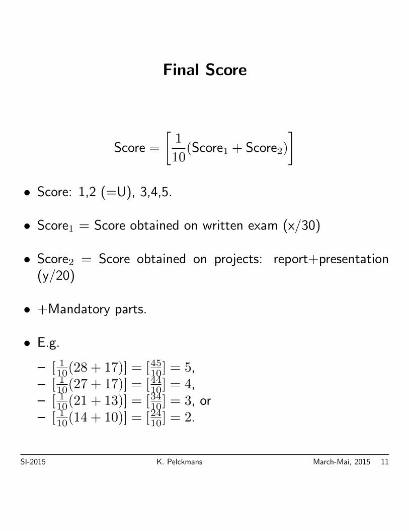
Final Score
Score =
[1
10(Score1 + Score2)
]• Score: 1,2 (=U), 3,4,5.
• Score1 = Score obtained on written exam (x/30)
• Score2 = Score obtained on projects: report+presentation(y/20)
• +Mandatory parts.
• E.g.
– [ 110(28 + 17)] = [4510] = 5,– [ 110(27 + 17)] = [4410] = 4,– [ 110(21 + 13)] = [3410] = 3, or– [ 110(14 + 10)] = [2410] = 2.
SI-2015 K. Pelckmans March-Mai, 2015 11
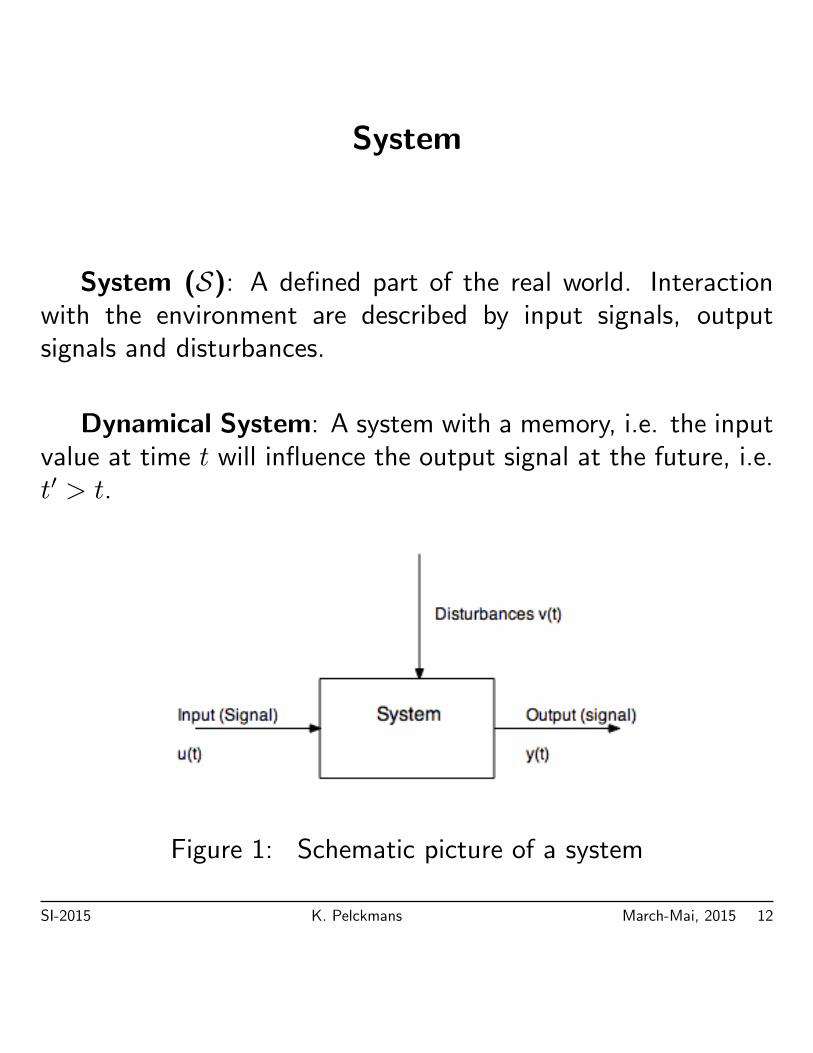
System
System (S): A defined part of the real world. Interactionwith the environment are described by input signals, outputsignals and disturbances.
Dynamical System: A system with a memory, i.e. the inputvalue at time t will influence the output signal at the future, i.e.t′ > t.
Figure 1: Schematic picture of a system
SI-2015 K. Pelckmans March-Mai, 2015 12
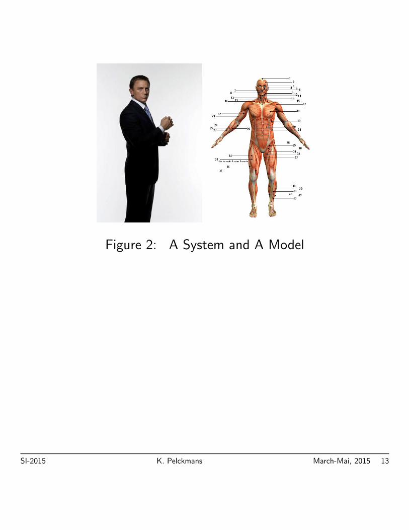
Figure 2: A System and A Model
SI-2015 K. Pelckmans March-Mai, 2015 13
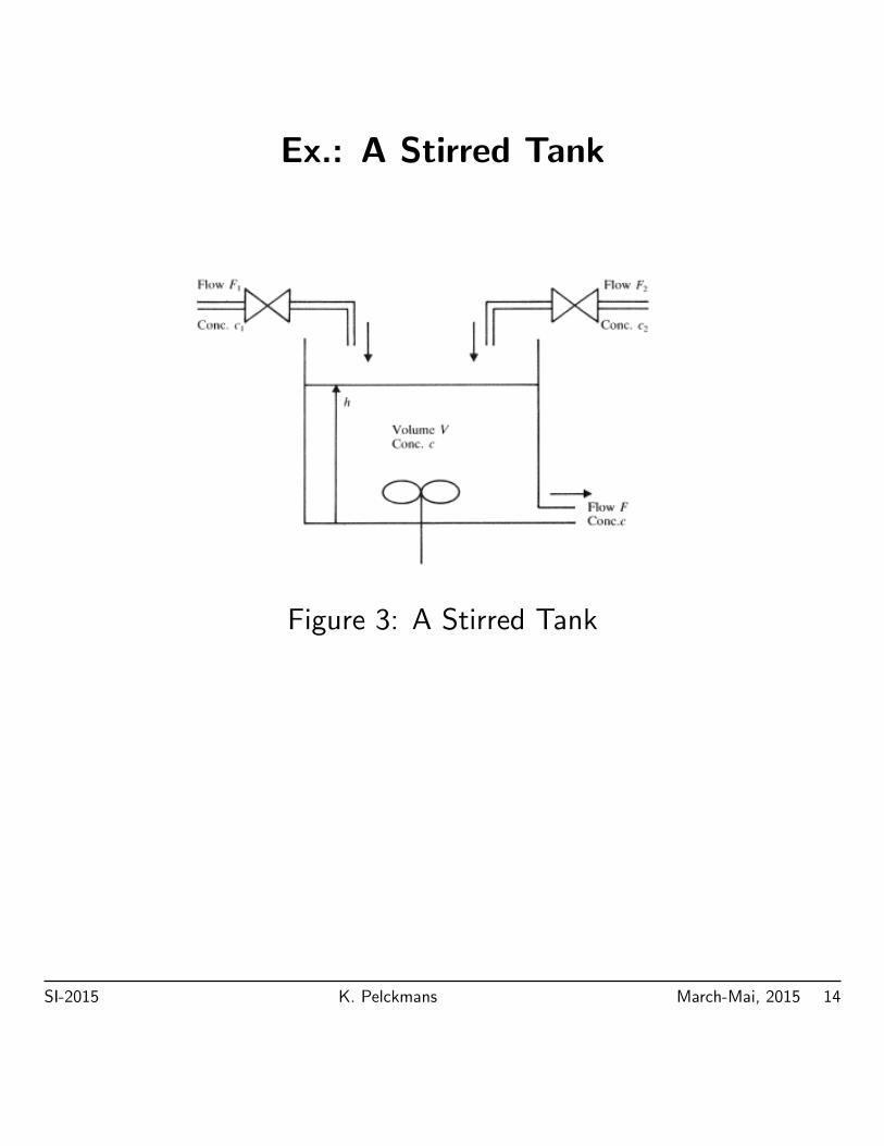
Ex.: A Stirred Tank
Figure 3: A Stirred Tank
SI-2015 K. Pelckmans March-Mai, 2015 14
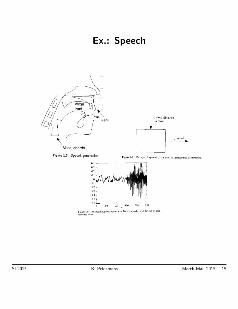
Ex.: Speech
SI-2015 K. Pelckmans March-Mai, 2015 15

Ex. and...
• Stock (Shock) Market
SI-2015 K. Pelckmans March-Mai, 2015 16

• Acoustic Noise Cancellation Headset (Adaptive filtering)
SI-2015 K. Pelckmans March-Mai, 2015 17

• Evolution of the Temperature in the world
SI-2015 K. Pelckmans March-Mai, 2015 18

• Construction (Strength)
SI-2015 K. Pelckmans March-Mai, 2015 19
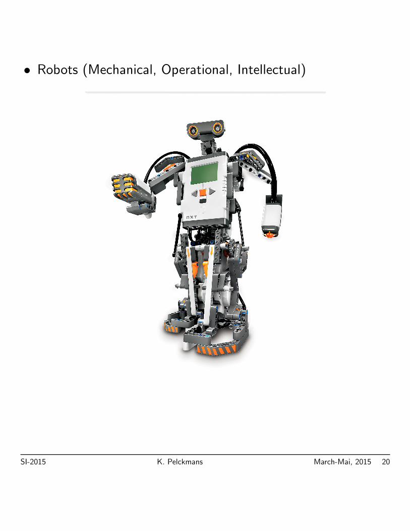
• Robots (Mechanical, Operational, Intellectual)
SI-2015 K. Pelckmans March-Mai, 2015 20
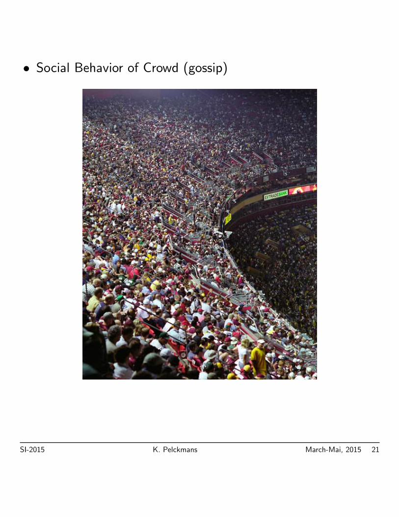
• Social Behavior of Crowd (gossip)
SI-2015 K. Pelckmans March-Mai, 2015 21
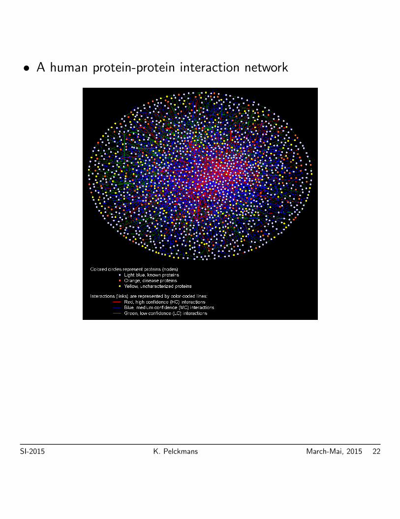
• A human protein-protein interaction network
SI-2015 K. Pelckmans March-Mai, 2015 22
Models
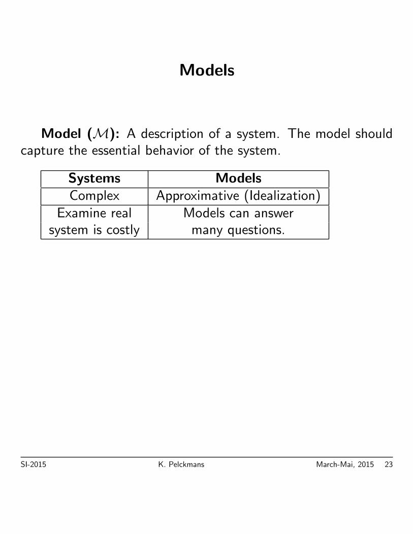
Model (M): A description of a system. The model shouldcapture the essential behavior of the system.
Systems ModelsComplex Approximative (Idealization)
Examine real Models can answersystem is costly many questions.
SI-2015 K. Pelckmans March-Mai, 2015 23
Applications
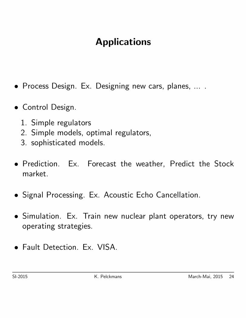
• Process Design. Ex. Designing new cars, planes, ... .
• Control Design.
1. Simple regulators2. Simple models, optimal regulators,3. sophisticated models.
• Prediction. Ex. Forecast the weather, Predict the Stockmarket.
• Signal Processing. Ex. Acoustic Echo Cancellation.
• Simulation. Ex. Train new nuclear plant operators, try newoperating strategies.
• Fault Detection. Ex. VISA.
SI-2015 K. Pelckmans March-Mai, 2015 24
Type of Models
• Mental, intuitive or verbal. Ex. Driving a car.
• Graphs and Tables. Ex. Bode plots and step responses.
• Math. models. Ex. Differential and Difference equations.
SI-2015 K. Pelckmans March-Mai, 2015 25
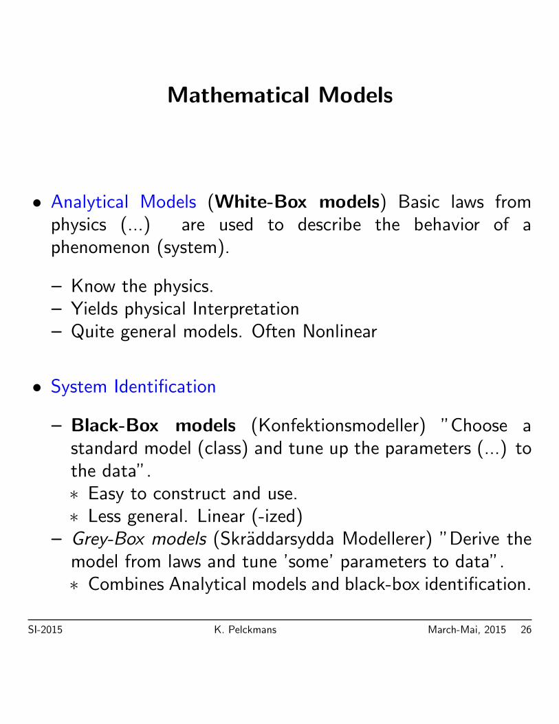
Mathematical Models
• Analytical Models (White-Box models) Basic laws fromphysics (...) are used to describe the behavior of aphenomenon (system).
– Know the physics.– Yields physical Interpretation– Quite general models. Often Nonlinear
• System Identification
– Black-Box models (Konfektionsmodeller) ”Choose astandard model (class) and tune up the parameters (...) tothe data”.∗ Easy to construct and use.∗ Less general. Linear (-ized)
– Grey-Box models (Skraddarsydda Modellerer) ”Derive themodel from laws and tune ’some’ parameters to data”.∗ Combines Analytical models and black-box identification.
SI-2015 K. Pelckmans March-Mai, 2015 26

Figure 4: White-, Black- and Grey-Box Models
SI-2015 K. Pelckmans March-Mai, 2015 27
Examples of Models
• Nonlinear vs. Linear (superposition principle):
”The net response at a given place and time caused bytwo or more stimuli is the sum of the responses whichwould have been caused by each stimulus individually.”(Wiki)
• Time-continuous versus Time-discrete
• Deterministic versus Stochastic
SI-2015 K. Pelckmans March-Mai, 2015 28
System Identification (SI)
Def. System Identification is the study of Modeling dynamicSystems from experimental data.
• Statistics, Systems Theory, Numerical Algebra.
• System Identification is art as much as science.
• Software available (MATLAB)
• – Estimation (Gauss (1809)),– Modern System Identification (Astrom and Bohlin (1965),
Ho and Kalman (1966)),– Recent System Identification (L. Ljung, 1977-1978)– Textbooks (Ljung 1987, Soderstrom and Stoica, 1989).
SI-2015 K. Pelckmans March-Mai, 2015 29
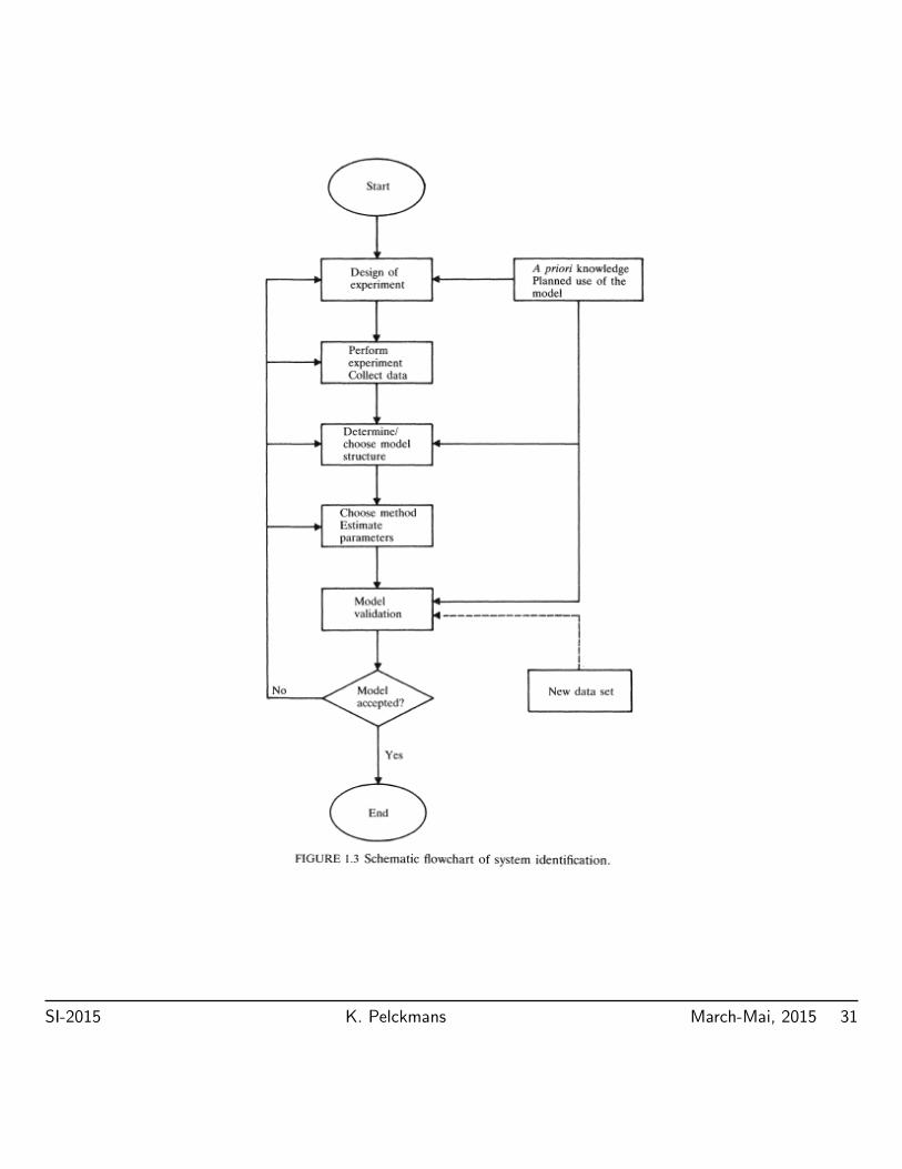
The System Identification Procedure
1. Collect Data. If possible choose the input signal such thatthe data is maximally informative. Display data, and try toget some intuition about the problem at hand.
2. Choose Model Structure. Use application knowledge andengineering intuition. Most important and most difficult step(don’t estimate what you know already)
3. Choose Identification Approach. How would a good modellook like?
4. Do. Choose best model in model structure (Optimization orestimation)
5. Model Validation. Is the model good enough for our purpose?
SI-2015 K. Pelckmans March-Mai, 2015 30
SI-2015 K. Pelckmans March-Mai, 2015 31
Typical Problems to Answer
• How to design the experiment. How much data samples tocollect?
• How to choose the model structure?
• How to deal with noise?
• How to measure the quality of a model?
• What is the purpose of the model?
• How do we handle nonlinear and time-varying effects?
SI-2015 K. Pelckmans March-Mai, 2015 32
System Identification Methods
• Non-parametric Methods. The results are (only) curves,tables, etc. These methods are simple to apply. They givebasic information about e.g. time delay, and time constantsof the system.
• Parametric Methods (SI) The results are values of theparameters in the model. These may provide better accuracy(more information), but are often computationally moredemanding.
SI-2015 K. Pelckmans March-Mai, 2015 33
Course Outline
(i) Overview.
(ii) Least Squares Rulez.
(iii) Models & Representations.
(iv) Stochastic Setup.
(v) Prediction Error Methods.
(vi) Model Selection and Validation.
(vii) Recursive Identification.
(viiii) SISO 2 MIMO.
(ix) Nonlinear Identification.
SI-2015 K. Pelckmans March-Mai, 2015 34
Conclusion
• System identification is the art of building mathematicalmodels of dynamical systems using experimental data. It isan iterative procedure.
– A real system is often very complex. A model is merely agood approximation.
– Data contain often noise, individual measurements areunreliable.
• Analytical methods versus system identification (white-,black-, grey box)
• Non-parametric versus Parametric Methods
• Procedure: (a) Collect data, (b) Choose Model Structure,(c) Determine the best model within a structure, (d) Modelvalidation.
SI-2015 K. Pelckmans March-Mai, 2015 35
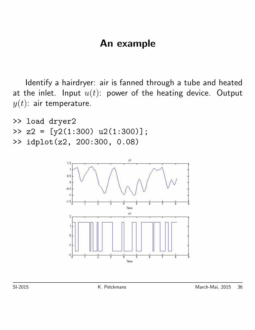
An example
Identify a hairdryer: air is fanned through a tube and heatedat the inlet. Input u(t): power of the heating device. Outputy(t): air temperature.
>> load dryer2
>> z2 = [y2(1:300) u2(1:300)];
>> idplot(z2, 200:300, 0.08)
SI-2015 K. Pelckmans March-Mai, 2015 36
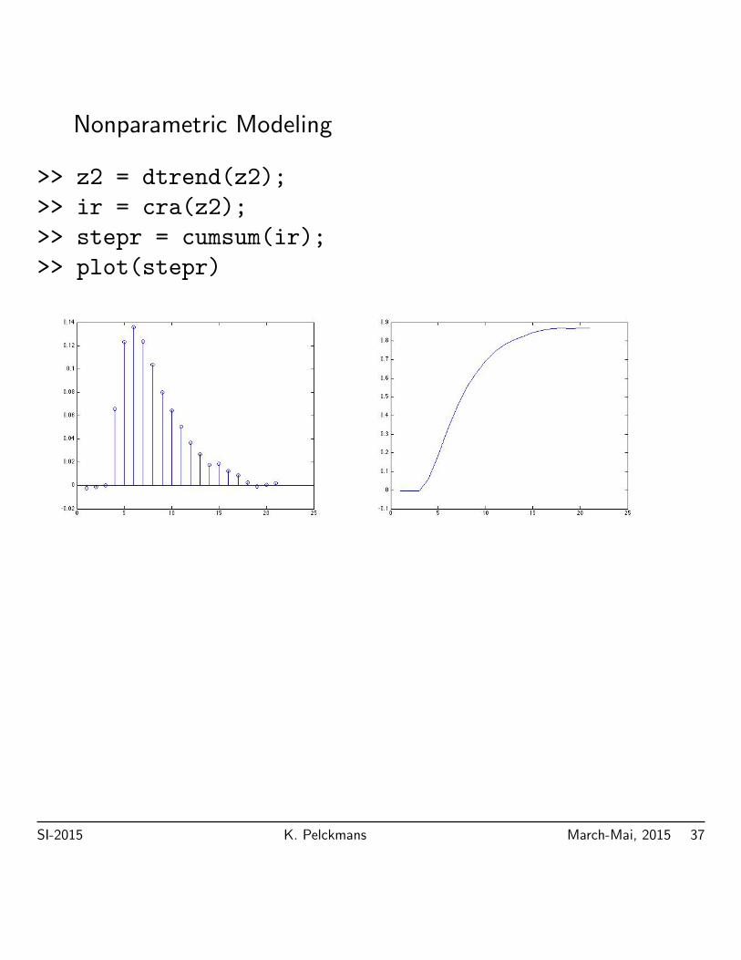
Nonparametric Modeling
>> z2 = dtrend(z2);
>> ir = cra(z2);
>> stepr = cumsum(ir);
>> plot(stepr)
SI-2015 K. Pelckmans March-Mai, 2015 37

Parametric modeling:
y(t) + a1y(t− 1) + a2y(t− 2) = b1u(t− 3) + b2u(t− 4)
>> model = arx(z2, [2 2 3]);
>> model = sett(model,0.08);
>> u = dtrend(u2(800:900));
>> y = dtrend(y2(800:900));
>> yh = idsim(u,model);
>> plot([yh y]);
SI-2015 K. Pelckmans March-Mai, 2015 38
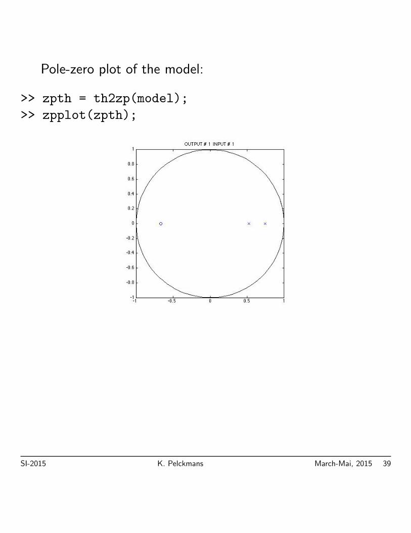
Pole-zero plot of the model:
>> zpth = th2zp(model);
>> zpplot(zpth);
SI-2015 K. Pelckmans March-Mai, 2015 39
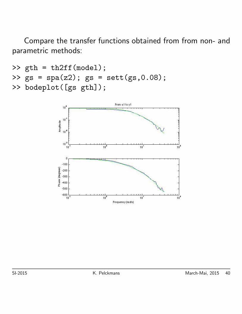
Compare the transfer functions obtained from from non- andparametric methods:
>> gth = th2ff(model);
>> gs = spa(z2); gs = sett(gs,0.08);
>> bodeplot([gs gth]);
SI-2015 K. Pelckmans March-Mai, 2015 40