Embed Size (px)
Citation preview
DESIGN, FABRICATION, AND CONTROL OF AN AUTONOMOUS SORTING
SYSTEM FOR NON-FERROUS METAL RECYLCING
By
CHRISTOPHER DIPAOLA
A thesis submitted to the
School of Graduate Studies
Rutgers, The State University of New Jersey
In partial fulfillment of the requirements
For the degree of
Master of Science
Graduate Program in Mechanical and Aerospace Engineering
Written under the direction of
Qingze Zou
And approved by
_____________________________________
_____________________________________
_____________________________________
_____________________________________
New Brunswick, New Jersey
October, 2019
ii
ABSTRACT OF THE THESIS
DESIGN, FABRICATION, AND CONTROL OF AN AUTONOMOUS SORTING
SYSTEM FOR NON-FERROUS METAL RECYLCING
by CHRISTOPHER DIPAOLA
Thesis Director:
Qingze Zou
Autonomous sorting systems are applied to pure and heterogeneous types of
metallic materials for recycling purposes with goals of efficiency in mind. The purpose of
this work was design and build an adjustable, automated, conveyor included sorting
system, and validate and evaluate its function and performance for sorting copper and
aluminum pieces in experiments. An overview of sorting methods in recycling, mining
and other industries are provided to examine the choices made in the design this system.
Fabrication steps were taken with facility factors in mind to build and mount the
individual components of the system. Challenges faced in the fabrication and operations
of the system are also considered. Individual components including compressed air, IR
detection, and computer controls are integrated together into the final system.
Demonstrations of the system components is done for each component separately, and
iii
then merged to form the finalized system. The design features the use of IR sensors to
identify a variety of non-uniform copper and aluminum pieces quickly, an array of relays
to open manifold outlets automatically, twenty solenoid valves with compressed air
actuation for timely control of air flow, and a computer-based data acquisition system for
real-time sensing and control under MATLAB-Simulink real-time software environment.
Safety features are added to the system so that accidents can be prevented while utilizing
the industrial components. This setup is built successfully and met the design expectation.
Experimental implementation to sort the copper and aluminum particles (each ranging
from 0.5in to 1in wide) shows that the system is very useful at detecting and shooting
materials at speeds from 15-45cm/s. This setup provides the capability to implement the
same methods industry uses and has the flexibility for prototyping future applications.
The experimental results show non-ferrous metal pieces can be successfully identified
and sorted.

iv
Acknowledgements
To my family who have been extremely supportive of me in all my academic endeavors.
To Professor Zou, who has given me many opportunities in his research as well his
guidance both as a graduate and undergraduate student.
To John Petrowski, Tom Calabrese, Darius Kozlowskiand, Joe Olshefski, and Sania
Sadhvani, for all the insight you provided with the machine shop, the refurbishing of the
workspace, and the resources you have shared with me both on campus and in industry.
To my Defense Committee, I thank you for your contribution towards my degree. I have
seen how involved you are at this university and in your own fields of study. The time
given to review my work, and provide feedback is much appreciated.
To the members of my research group and H.S.G. INC. for providing the project for
which I am working, and for providing me extra guidance in this project. Specifically,
Yuguang, Tianwei, Parth, Fan, Birju, Jingren, Jiaorong, Guang, Guangze, and Birju.
v
TABLE OF CONTENTS
ABSTRACT OF THE THESIS .......................................................................................... ii
Acknowledgements ............................................................................................................ iv
Table of Contents .................................................................................................................v
List of Tables .................................................................................................................... vii
List of Figures .................................................................................................................. viii
1. Introduction ......................................................................................................................1
1.1. Overview of Industrial Sorting ...............................................................................1
1.1.1. Purpose for the Project: Inspiration from Zero Waste ...................................1
1.1.2. Overview of Industrial Recycling ..................................................................5
1.1.3. Conveyor Sorting Schemes and their Limits ................................................7
1.1.4. Facility Requirements ..................................................................................12
1.2. Design Motivations and Considerations ...............................................................14
1.3. Integrated Final Design .........................................................................................19
1.4. Project Planning and Challenges ..........................................................................21
2. Equipment, Fabrication, and Implementation ................................................................24
2.1. SJF Conveyor ........................................................................................................24
2.1.1. Conveyor Specifications ..............................................................................24
2.1.2. Motor Drive: Powerflex 520 .......................................................................25
2.1.3. Belt Installation ...........................................................................................27
2.2. Framing Components ...........................................................................................28
2.2.1. Exterior Frame ............................................................................................28
2.2.1. Sorting Chamber .........................................................................................30
2.3. Compressed Air Components ...............................................................................30
2.3.1. Interior Framing and Case ...........................................................................30
2.3.2. Solenoid Valves and Jets .............................................................................34
2.3.3. Eagle EA 5000 Compressor ........................................................................36
2.4. Sensing Methods ...................................................................................................38
vi
2.5. Control Scheme .....................................................................................................39
2.5.1. 5 V Relay Modules ......................................................................................39
2.5.2. NI PCIE 6259 DAQ Card ............................................................................39
2.5.3. DELL Optiplex 3060 Computers .................................................................41
2.6. Safety and Building Code Considerations ............................................................42
3. Software Wiring, and Setup ...........................................................................................43
3.1. Simulink real-time Requirements .........................................................................43
3.1.1. Key Components for Connection.................................................................43
3.1.2. Calibration of DAQ Card to Simulink Blocks .............................................45
3.2. Signal Diagrams ....................................................................................................47
3.3. Control Schemes ...................................................................................................50
4. Operations and Testing ..................................................................................................53
4.1. Individual Components .........................................................................................53
4.1.1. Conveyor Flow.............................................................................................53
4.1.2. Compressed Air Shooting ............................................................................56
4.1.3. Sensing Calibrations ....................................................................................58
4.2. Modifications for Integrated Testing ....................................................................62
4.2.1. System Limitations ......................................................................................62
4.2.2. Final System Testing....................................................................................63
4.3. Future Improvements and Applications ................................................................66
5. Conclusions ....................................................................................................................68
Appendix A. MATLAB Codes References .......................................................................70
Appendix B. CAD Drawings for Design .......................................................................... 79
References ..........................................................................................................................81

vii
LIST OF TABLES
Table 1. Examples of Sorting Methods used in MSFs.........................................................7
Table 2. Examples Automated Sorting on a Conveyor......................................................10
Table 3. Considerations Necessary Prior to Equipment Purchasing..................................22
Table 4. Sample Angle Orientations of Manifold Case .....................................................31
Table 5. DAQ Card Wiring and Simulink Block Calibrations ..........................................46
Table 6. Sensor to Valve Correspondence, as positioned in setup indicates .....................55
viii
LIST OF ILLUSTRATIONS
Figure 1. Sample Pieces of Copper and Aluminum for Experimentation ...........................4
Figure 2. A Sample Material Recovery Facility (MRF) Operation Line .............................6
Figure 3 Reflective Properties of some Non-ferrous metals ............................................... 9
Figure 4. Preliminary Design: Mechanism and Drawing ..................................................15
Figure 5a. Engineering Sketch of First Design ..................................................................16
Figure 5b. Sketch of Second Design ..................................................................................16
Figure 6. TOMRA Industries Vision Sorting Method .......................................................17
Figure 7. MSS Industries Sorting Configurations .............................................................18
Figure 8. Third Design with Compressed Air ....................................................................19
Figure 8. Final Design........................................................................................................21
Figure 10. Conveyor Before and After Installation ...........................................................24
Figure 11. Setting and Control Panel for PLC ...................................................................26
Figure 12a. Final Exterior Frame .......................................................................................29
Figure 12b. Framing Accessories ......................................................................................29
Figure 13. Final Sorting Chamber .....................................................................................30
Figure 14. Interior Frame and Manifold Mount Images ....................................................31
Figure 15. MSV8 10 Manifold...........................................................................................32
Figure 16. Manifold Case Finished Product ......................................................................33
Figure 17. Solenoid Valves, Diagram and Flow Specifications ........................................35
Figure 18. Eagle EA 5000 Air Compressor .......................................................................37
Figure 19. Wired IR Array, and Mounting Board ............................................................38
Figure 20. Wired 5V Relay Terminals ...............................................................................39
Figure 21. PCIE 6259 Installed and Attached I/O Board Terminals .................................40
Figure 22. Computer Setup Prior to Conveyor System Integration ...................................41
Figure 23. Safety Lock Box ...............................................................................................42
Figure 24. SLRT Boot Configuration ................................................................................43
Figure 25. Electrical Circuit for Solenoid Valves ..............................................................47
ix
Figure 26. Fundamental Operation ....................................................................................48
Figure 27. Second Subsystem to delay off switch .............................................................49
Figure 28. Final Conveyor-Sensor-Valve-Power Block Diagram .....................................51
Figure 29. Example Signal Plots of Conveyor with Pieces sent thorough system ............52
Figure 30a. Comparison between Measured Conveyor Speed and Actual Speed .............54
Figure 30b. Comparison of Required Time delay using Measured Conveyor Speed .......54
Figure 31. Air Compressor Pressure Readings after Valve Opening ................................57
Figure 32a. Conveyor Speed 25FPM, 0.05 sample time ...................................................58
Figure 32b. Conveyor Speed 25FPM, 0.05 sample time (after sensitivity adjustment) ....58
Figure 32c. Conveyor Speed 100FPM, 0.05 sample time .................................................59
Figure 32d. Conveyor Speed 100FPM, 0.01 sample time .................................................59
Figure 33. IR Sensor Calibration of Aluminum.................................................................60
Figure 34. Final Design......................................................................................................64
Figure 35. Sensor and Valve Readings with Detecting Counters ......................................64
Figure 36. Test Piece Selection ..........................................................................................65
Figure 37. Drawing of Manifold Case ...............................................................................79
Figure 38. Conveyor Specifications ...................................................................................80

1
1. Introduction
1.1 Overview of Industrial Sorting
1.1.1. Purpose for the Project: Inspiration from Zero Waste
In recent years, there has been a call for “zero waste” for conservation purposes as
well as automated manufacturing purposes to optimize the use of natural resources and
make them continuously reusable. With world population estimated to grow, it is
essential to make efficient use of everyday items that end up going to a recycling center
or a landfill at the end of its life [1]. In most cases these items are a composition of a
variety of materials which makes repurposing them somewhat of a challenge because
they can lose value, either in their material properties, or in general purpose. For
example, the plastics we use every day in containers or on tops of bottles can be recycled
in some cases, but only through a certain number of life cycles. When contaminated with
food waste, recycling is out of the question. As a result, most plastics end up in landfills,
compost, or in the sea [1, 2]. So, there are some cases where it is near impossible to
effectively recycle some of these everyday items. However, sorting is simpler with
materials such as metals which the same fragment can be reused in numerous products
and life cycles. By fabricating and testing a simplified, adjustable metal sorting system
the processes used by can be better understood and demonstrated. Future testing and
implementation of said system can be done to potentially achieve more effective sorting,
recycling or general manufacturing methods.
Sorting in this sense is the act of separating materials by certain characteristics using
control techniques in a sequential manner such that they can be distinguished. Sorting is
divided into two types “ordering”, and “categorizing.” Ordering is a type of sorting in
2
which item order matters; categorizing means the order of items is not important
compared to the properties of the items [3]. Shipping would have concern with the timing
of their shipments, and so ordering would have a place in the facility. However, with
recycling applications, all the material goes through and the order is disregarded.
Spending time to order the material is a waste when concerned with generating larger
output quantities. Thus, this work will only be concerned with the categorizing form of
sorting.
Mining and Agriculture facilities have uses for categorizing schemes as well. In
mining, segments of ore are sent through sensors which grade the ore and determine if it
is of high value or low value based on its qualities. Then by sorting, minerals and metals
such as copper, coal, and even diamonds and gold can be easily recovered separately [4].
In agriculture, similar technology is implemented for early defect detection, visual defect
detection, and grading, and sorting crops [5]. This enables them to prevent infected seeds,
processed crop, or even fruits from affecting uninfected batches, which a reseller would
find undesirable. As diverse as these applications are they all act on the same principle:
increase the value of their finished items, while removing the parts that the general
population would find undesirable, and do so in a fast, efficient way.
This work is inspired by the idea that by qualifying every piece of metal that travels
along the conveyor more thoroughly, it is possible to determine more efficient means of
sorting the pieces, and potentially finding uses for the undesirable parts of said pieces that
were discarded previously. In terms of creating zero waste sorting methodology is not as
effective as perceived, because it implies removing parts that have zero value, which is
considered waste. For example, only 5% of the world’s plastics is recycled in said

3
facilitates, meaning 95% still ends up in landfills, compost, or the oceans [1]. To achieve
zero waste, the processing line must be able to find use for the undesirable parts of items
that flow through a sorting line and be able to separate each component more precisely.
Furthermore, the desired sensing, and separating capabilities must be quite precise.
Material that traverse through a recycling line has properties unique to its type, and
corresponding engineering purposes in its final form. Such properties can be used for
scientifically identifying each piece and then separating them for sorting. Such
characteristics can include but are not limited to weight, density, temperature, electrical
conductivity, magnetic interactivity, color, odor, and even a combination of such
principles. Because we desire a setup that can work with a variety of accessories, it is
beneficial to begin with a system that is easy to fabricate and test.
Metal sorting is by far the easiest for this idea because metals are the easiest to detect,
by identifying its color or density properties, and so can easily be sorted. From a
recycling standpoint, they can be recycled indefinitely, and so always has a satisfactory
purpose. On the other hand, plastics on the other hand can only be recycled once or twice
[6]. Metallic metals such as steels are even easier to distinguish via magnetic properties.
For our purposes, the design and fabrication will be for non-ferrous metallic materials,
specifically pure pieces of copper and aluminum.
Pieces of copper and aluminum were provided by HSG INC and delivered from the
computer science department in Rutgers New Brunswick. There are three types of pieces
to work with. The first is pure copper, second is pure aluminum, the third is a grinded
mixture of the two. The copper with density higher that of the aluminum are about the
same size, whereas the aluminum shavings are very small in comparison. However, the
4
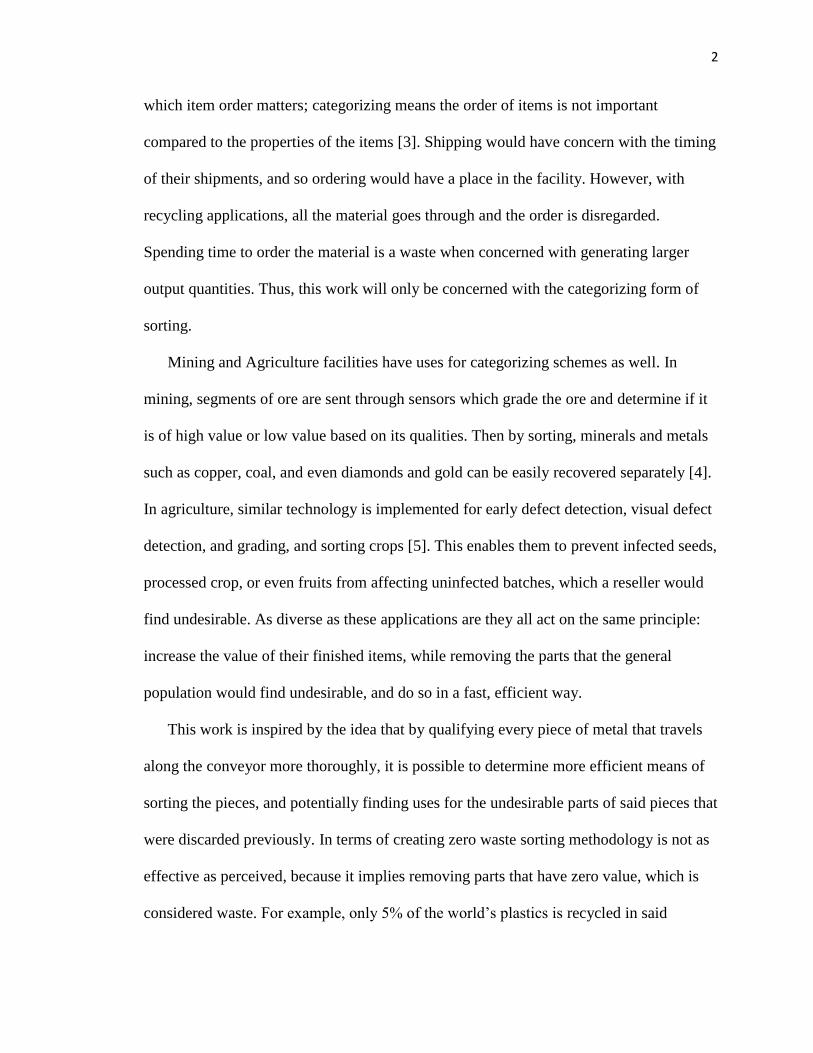
aluminum shavings can be piled together to make larger sized pieces, and so has some
flexibility to modify size and shape for experimental purposes. The aluminum shavings
provide means of varying the compositions of the mixture pieces, but only one shaving of
aluminum on the conveyor will be difficult compared to the regular sized pieces.
Fig. 1. Sample Pieces for Experimentation: from right to left, piece of pure aluminum,
aluminum shavings, pure copper, and mixture of aluminum and copper on conveyor belt.
Purity is an important assumption in this design because most of the time, materials
that move through a recycling or mining plant have a more complex composition. Pure
materials have uniform chemical composition, and mechanical properties throughout the
volume of the body. In theory, this provides optimal sorting capability because then all
the materials on the conveyor are completely known. However, in plastic recycling and
other applications, there are rarely true “pure” materials which makes sorting accurately a
constant challenge [1,6]. Our metal pieces can be grouped together either juxtaposed
lengthwise or widthwise or grinded together. In these cases, effective sorting proves to be
even more challenging.
Sorting efficiency is defined as the amount of material mass sorted correctly over the
total mass. Industries that use sorting such as recycling, and mining want higher
efficiencies in their automated systems while moving products as fast as possible.
5
Assuming this is most of the material, the mass of what was mislabeled or sorted
incorrectly will be easier to quantify. Below describes this relationship with “𝜂” for
efficiency, and m for mass.
𝜂 =𝑚𝑠𝑜𝑟𝑡𝑒𝑑
𝑚𝑡ℎ𝑟𝑜𝑢𝑔ℎ𝑝𝑢𝑡100% (1)
From an industrial standpoint, the faster and more accurate the sort, the better. The
conveyor adds a speed component to the sorting system, as human hands sorting bin to
bin can be tedious labors. However, the human eye that can distinguish materials and sort
more accurately through experience with products, which is why some facilities continue
to use manual labor as an option. In creating this design, the intent is to have a system
that has potential to achieve high efficiencies.
1.1.2. Overview of Industrial Recycling
Recycling is accomplished in a variety of different ways, but the main floor processes
are all done in the same order. There are two types of streams from which recycling
facilities receive their throughput: single stream, and dual stream. Single stream is where
all recyclable materials, glass, plastic containers, paper, metal and more are picked up
and then sorted at the facility. Dual stream is where fiber components are separated by
households from the plastics, cans, and glass [7]. Most locations use dual stream, as it
enables faster sorting from start to finish in their local facilities.
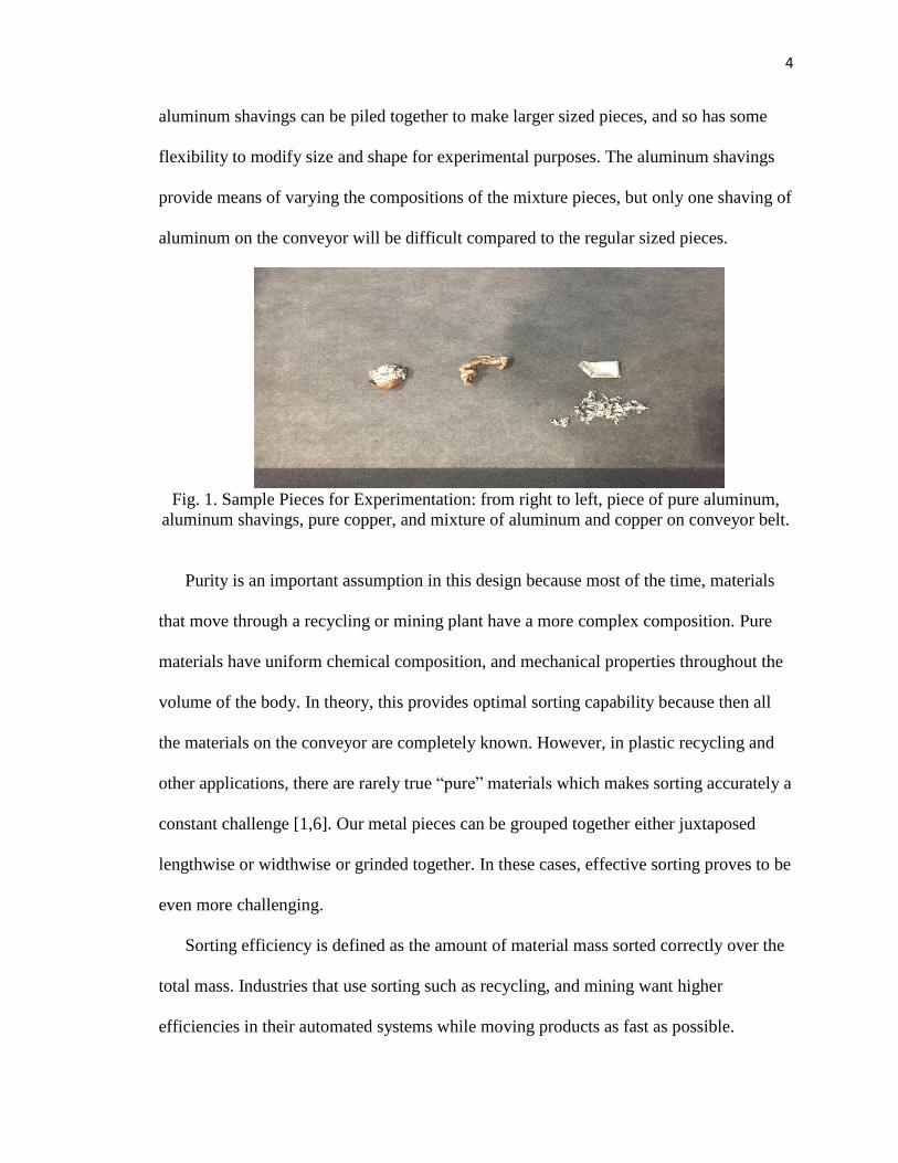
The diagram on the next page shows how the recycling process is run from start to
finish. The process begins with collection of materials from scrapyards, homes,
businesses and other localized areas. The lot is then placed onto a series of conveyors,
then processed and sorted one by one categorically to create the desired output. In the
6
facility described, first non-recyclable materials are removed by labor, then fibrous
material like paper and cardboard, then glassy material, then magnetic material, then
metals, then finally plastics. Finally, once processing is complete, the output can be
processed (grinded, or hammered), then redistributed as useful materials to the market
[8].
Fig. 2. A Sample Material Recovery Facility (MRF) Operation Line [8].
In every stage of the recycling process previously addressed there is a sorting
mechanism that removes one material type from the larger pile. Fibrous papers for
example are lighter than the rest of the materials moving through enabling them to be
sorted by an acceleration, which would then force the heavier materials to fall in
comparison [8]. Another example is using eddy currents to electrically accelerate metals
7
while not accelerating the plastics. Regardless of the stage, the key component to the
sorting control process is the material properties of the throughput.
To autonomously sort such material, these properties must be examined accurately on
each item, and sorted using a mechanism best suited for the application. Direct sorting is
the term for sorting in this manner, whereas indirect sorting is based on simple detection
of materials without examining their properties to employ machinery to move them from
the rest of the set [9]. Both types of sorting are utilized in a variety of applications with a
variety of materials in the recycling process. For example, because some materials are
magnetic, a magnet can detect and sort them from the remainder of the pile. For our
purposes, showing the efficiency of an indirect sorting of similar non-ferrous metals is
desired and enough for demonstrating system capabilities.
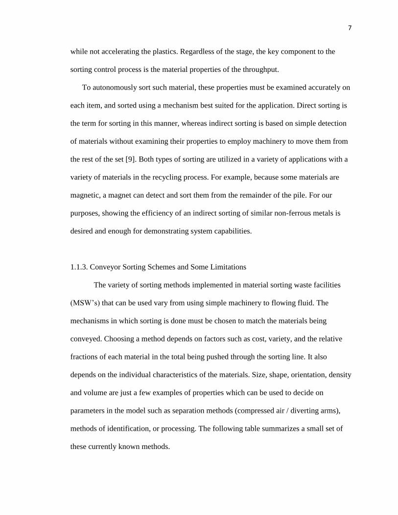
1.1.3. Conveyor Sorting Schemes and Some Limitations
The variety of sorting methods implemented in material sorting waste facilities
(MSW’s) that can be used vary from using simple machinery to flowing fluid. The
mechanisms in which sorting is done must be chosen to match the materials being
conveyed. Choosing a method depends on factors such as cost, variety, and the relative
fractions of each material in the total being pushed through the sorting line. It also
depends on the individual characteristics of the materials. Size, shape, orientation, density
and volume are just a few examples of properties which can be used to decide on
parameters in the model such as separation methods (compressed air / diverting arms),
methods of identification, or processing. The following table summarizes a small set of
these currently known methods.
8
Material
Class
Magnetic
Drum
Eddy
Current
Hydro-
cyclone
Air
Separator
Jigging Optical Sort
Ferrous
Metals
Y N N N Y N
Non-
Ferrous
Metals
N Y N N Y Y
Plastic
N N Y Y Y Y
Glass
N N N N N Y
Table 1. Examples of Sorting Methods in MSW facilities [9].
Knowing how to sort materials into their respective classes is enough for the first part
of the recycling process. The next part will be to separate materials with the same
classification such as copper and aluminum, which are both non-ferrous metals. In this
case, more than electrical properties will be necessary for the sort. For an autonomous
sort, more sophisticated sensing will be required to detect other differences between the
two. More specialized sorting can be done in some cases by hand such as in waste
removal in the first stage of a recycling plant [8], but in other cases automatically via
computer vision or various sensors. Computer vision, and light spectroscopy are two
other methods for distinguishing copper and aluminum in this way.
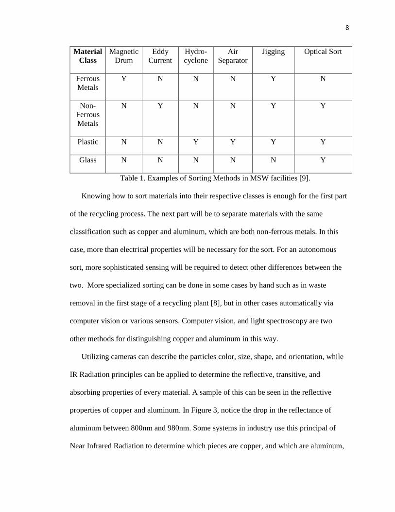
Utilizing cameras can describe the particles color, size, shape, and orientation, while
IR Radiation principles can be applied to determine the reflective, transitive, and
absorbing properties of every material. A sample of this can be seen in the reflective
properties of copper and aluminum. In Figure 3, notice the drop in the reflectance of
aluminum between 800nm and 980nm. Some systems in industry use this principal of
Near Infrared Radiation to determine which pieces are copper, and which are aluminum,
9
and then can separate them into two specific piles. Whereas this method requires more
sophisticated sensors, it works better when separating materials similar in size, shape, and
color, properties that a camera vision system may not necessarily detect.
Figure 3: Reflective properties of some non-ferrous metals [10].
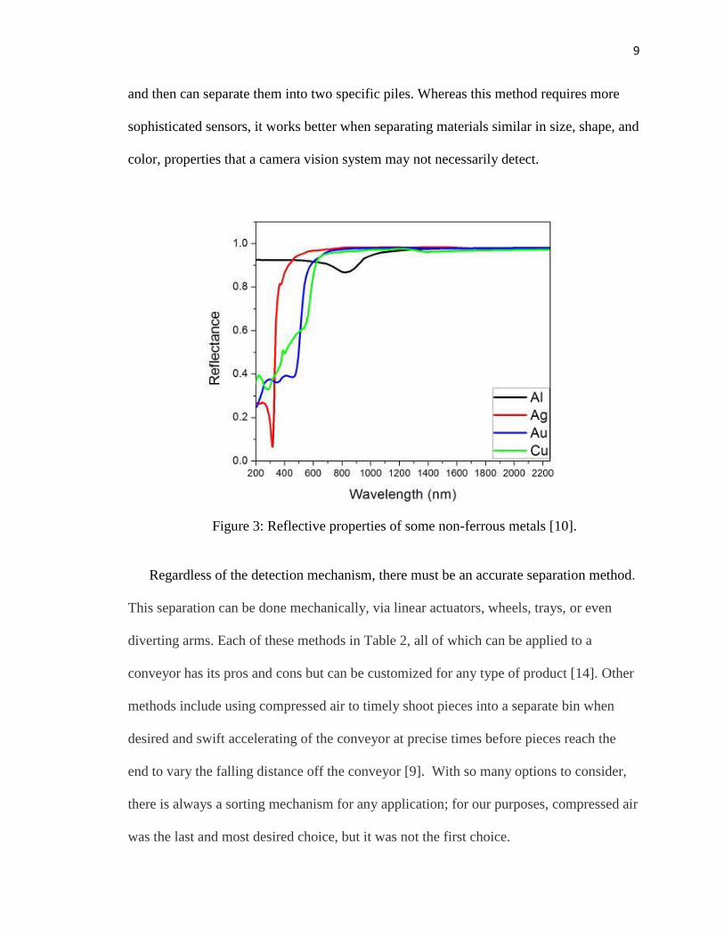
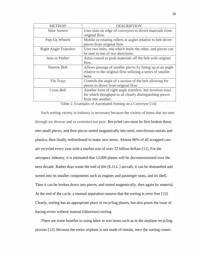
Regardless of the detection mechanism, there must be an accurate separation method.
This separation can be done mechanically, via linear actuators, wheels, trays, or even
diverting arms. Each of these methods in Table 2, all of which can be applied to a
conveyor has its pros and cons but can be customized for any type of product [14]. Other
methods include using compressed air to timely shoot pieces into a separate bin when
desired and swift accelerating of the conveyor at precise times before pieces reach the
end to vary the falling distance off the conveyor [9]. With so many options to consider,
there is always a sorting mechanism for any application; for our purposes, compressed air
was the last and most desired choice, but it was not the first choice.
10
METHOD DESCRIPTION
Shoe Sorters Uses slats on edge of conveyors to divert materials from
original flow.
Pop-Up Wheels Mobile or rotating rollers at angles relative to belt divert
pieces from original flow
Right Angle Transfers Uses two belts, one which feeds the other, and pieces can
be sent in one of two directions.
Arm or Pusher Arms extend to push materials off the belt with original
flow.
Narrow Belt Allows passage of smaller pieces by lining up at an angle
relative to the original flow utilizing a series of smaller
belts.
Tilt Trays Controls the angle of a section of the belt allowing for
pieces to divert from original flow.
Cross Belt Another form of right angle transfers, but involves trays
for which thoughput to sit clearly distinguishing pieces
from one another.
Table 2. Examples of Automated Sorting on a Conveyor [14]
Such sorting variety in industry is necessary because the variety of items that are sent
through are diverse and in extension not pure. Recycled cars must be first broken down
into small pieces, and then pieces sorted magnetically into steel, non-ferrous metals and
plastics, then finally redistributed to make new items. Almost 86% of all scrapped cars
are recycled every year with a market size of over 32 billion dollars [11]. For the
aerospace industry, it is estimated that 12,000 planes will be decommissioned over the
next decade. Rather than waste the end of life (E.O.L.) aircraft, it can be dismantled and
sorted into its smaller components such as engines and passenger seats, and its shell.
Then it can be broken down into pieces, and sorted magnetically, then again by material.
At the end of the cycle, a manual separation ensures that the sorting is error free [12].
Clearly, sorting has an appropriate place in recycling planes, but also poses the issue of
having errors without manual (laborious) sorting.
There are some benefits to using labor to sort items such as in the airplane recycling
process [12]. Because the entire airplane is not made of metals, once the sorting comes

11
down to plastics, glasses, and other less distinguishable materials, some issues with
automated sorting can arise. Shipping companies such as Amazon still use manual labor
to manually sort and deliver goods for orders [13]. This makes sense due to their large
variety of products; organization and computerized positions of items must be exact for
items to be located efficiently. When dealing with either a large variety of materials, or
materials with properties that cannot be distinguished by an automated process, manual
sorting is necessary to have an idealistic system where items are processed quickly, and
accurately according to consumer needs. In general, it seems that all aspects of conveyed
sorting still require some action from labor, leaving room for improvements in
autonomous sorting versus labor.
Another big issue with automated sorting systems are “the inability to incorporate
flexibility into its design [15].” Flexibility here means that while every sorting system is
designed particularly for one company needs, it cannot handle certain other types of
materials. For each material, there are corresponding sorting methods, but one system
cannot necessarily sort all materials at one time. The most flexible method is a series of
sorting systems, one after the other. However, a setup like this requires a plethora of
machinery and isn’t as useful when the sorting is for pure items.
Other problems in facilities occur when there is a large variety of materials to sort,
such as in Amazon where they rely on labor in the mid-section of their sorting line to
process orders [13]. Labor is not as economically viable but only when the sorting is
simple, such as in the ideal case where only one sorting system is required for two types
of materials. There is room in industry for more information on more complex
autonomous sorting, such as with plastics. Plastics are divided into 7 categories by

12
recycling terminology, but there are two types of plastics, thermoplastics, and thermosets.
Thermoplastics can be melted and remade into production with new products, while
thermosets cannot be melted again; between the two only thermoplastics are recyclable
[2]. In some cases, plastics can be separated from one another, but not in others. Coffee
cups have a thin layer of polypropylene (PPL) on the inside, while the outside is plastic.
The exterior and interior cannot be separated without a specifically designed machine. In
most cases, plastic/paper cups are not recycled and simply sent to landfill. Some other
limits exist with sorting materials in today’s markets. The world has seen an increase in
plastic recycling to approximately 20% of all plastic waste, suggesting that more efficient
recovery of plastic needs to be applied in the future [16,17]. Practically any multi-
material item presents an ongoing problem in recycling, even if it is simply food stained
containers.
With all these limitations, and considerations it is still possible to find systems in
industry sorting at a high efficiency such as TOMRA and MSS and with items such as
copper and aluminum, efficient sorting (up to 98%) is recorded [18,19]. Metals that can
be grinded into small chunks, can be sorted piece by piece accurately using a variety of
methods. This is what we intend to show in the first stage of using the system which has
been designed and fabricated.
1.1.4 Facility and Design Requirements
Distinguishing items from one another on the conveyor is not the only thing to
consider with automated sorting. Spacing between items, and speed of the conveyor can
affect the overall usefulness and the final output of the system. Having pieces on a

13
conveyor too close together can be problematic for sensors. Depending on the resolution,
there can be scenarios where different pieces are sorted together, causing a contaminated
output to exist. Furthermore, if the speed is large enough, then sensors can potentially
miss a reading, and create a situation where pieces are overlooked instead of sorted.
For our system, pieces of different ranging sizes from shavings to 1in pieces are to be
conveyed over the length of the conveyor. For testing purposes, the conveyor is required
to have a width of at least 2ft, allowing for more than one piece to move through at a
time. It must also be long enough (at least 10ft) to allow for a variety of applications and
additions. To attach accessories, a frame is to be built, and allow for customizations. It
was also desired for the conveyor to work in conjunction with an industrial robotic arm
adjacent to the conveyor. The speed of the conveyor was required to be variable to enable
testing at slow speeds and run at higher speeds as well. In choosing the conveyor, sorting
system, and sensing methods, multiple options were considered.
Safety must also be a consideration when working with factory grade equipment. The
conveyor has many moving parts, all controlled by a Programmable Logic Controller
(PLC), which connects the motor, chain, rollers, and belt. Wires for the motor, sensors,
cameras, and control system must also be assembled with caution. It is also desired to
prevent mis-usage of the conveyor by unauthorized personnel, and usable with a robot
arm that was installed in conjunction with the conveyor. Fencing, and guarding were both
proposed options here. Electricity (240-480V outlet is required for the conveyor motor),
and the facility needs to have enough outlets for computers, and system accessories with
which to be powered. Included with this electricity was two emergency stops, to be able
to stop the conveyor in the event of an emergency. Having a wide conveyor, coordination
14
of lab space with other industry grade equipment is essential, with excess space
maintenance purposes. All external work such as assembling and transporting the
conveyor, as well as installing enough power for the machine was managed, and
completed successfully. This was done by certified rigors and electricians respectively.
1.2.Design Motivations and Considerations
Although there is a substantial quantity of firms and online references on metallic
sorting systems, few offer the exact makings of its control operations, and even fewer are
sophisticated enough to handle an extensive variety of materials at one single time, so
that it can be reused in multiple sorting scenarios. Buying a conveyor sorting system from
example MSS INC, there are numerous choices of purchases. Some systems are used for
scrap metal sorting and mining, while others are for agriculture seeds with defects, and
even some are for sorting plastics. Even though the metal sorting and recycling methods
of today are well understood, it makes sense to study current systems and see in what
ways there can be improvements to the status quo. In doing so, we keep our system able
to handle a variety of adjustments moving forward.
Our first proposed design was based on mechanical sorting using diverting arms and
wheel spacing. This design was created via CAD software in the computer labs at the
university. Pieces at the end of the conveyor come down and are sorted into rows by
stationary arms. From there, wheels space pieces out for later swiping by arms at the end
of the conveyor. The result is 6 uniformly separated rows, three of copper and aluminum
respectively. A frame is built using metallic struts to form a flexible accessory mount for
the conveyor. Anodized aluminum was chosen for the material frame because it is
15
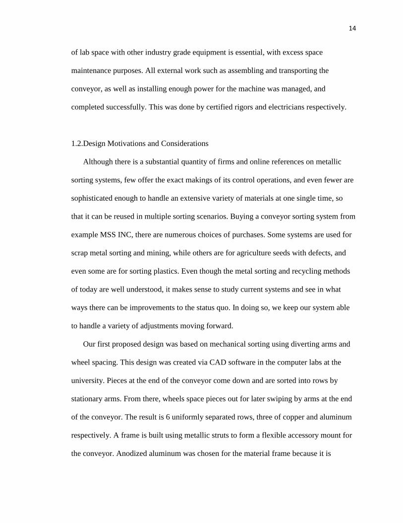
lightweight, and easier to mechanically adjust compared to other metals such as titanium,
is not magnetic, and not corrosive.
Fig. 4. Preliminary Design and Mechanical Mechanism and Drawing
Some issues here include the fact that there needs to be motors for all the wheels, the
wheels must be enough to space pieces out well, which is a challenge with irregular sized
pieces. The moving arms must also be small but powerful enough to swipe pieces side to
side, but accurately so that there is no overlap between rows. Also, guiders, moving arms,
and wheels must be placed a distance above the conveyor to prevent rubbing against the
belt, which can affect belt speed with drag. It is challenging to have only three rows of
throughput and a large speed to efficiently sort all the specimens with this design.
Having more accessories close to the belt like this limits ability to accessorize the
system later. Wheels on conveyors typically spin against the flow of the belt and can
cause pieces to pile up in the wheel areas. When using guides and setups that slow down
material is that if the pieces cannot move forward, the tendency is for them to pile up on
top of one another. If the pieces are uniform in shape and can approach the sorting in
rows, then this is not an issue. However, with small fragments of metals in a variety of
sizes, this design can easily cause pieces to pile up. Thus, a new proposal was made:
16
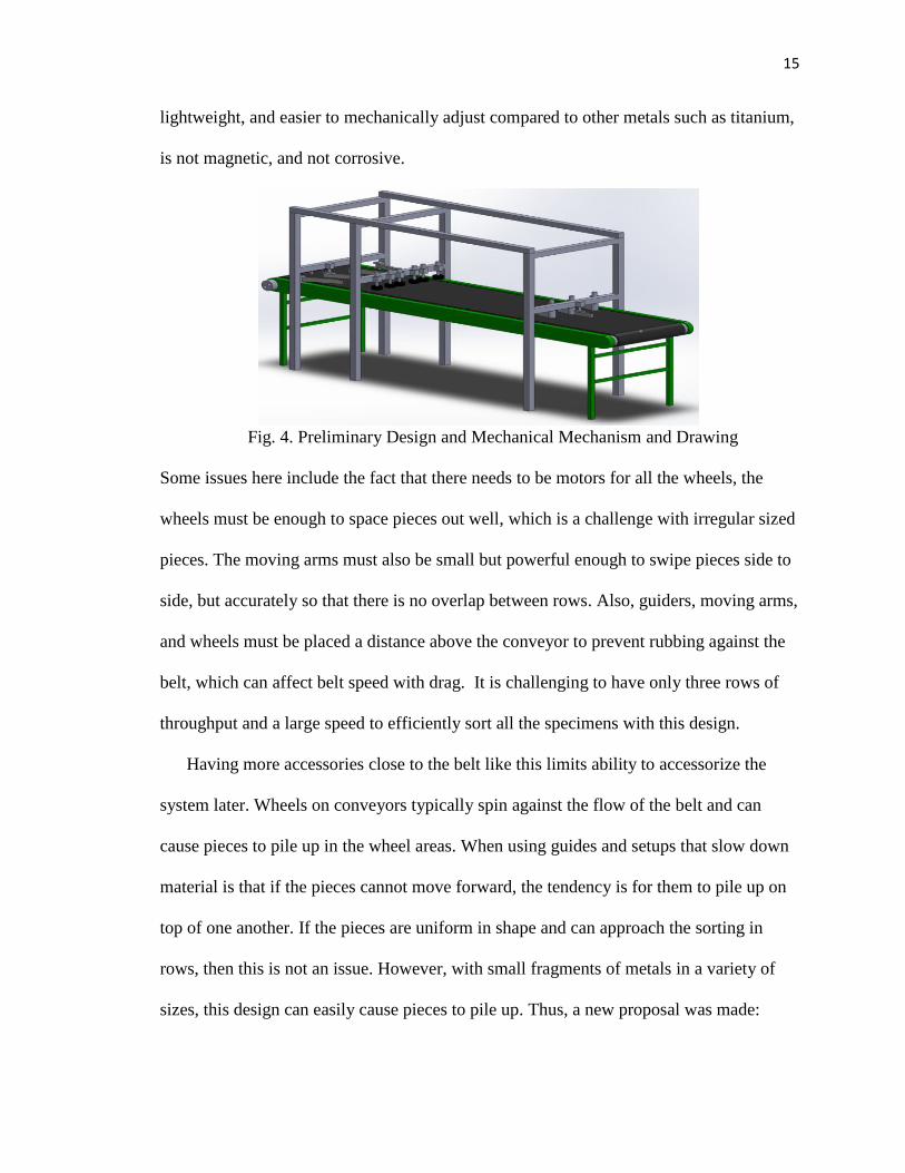
Fig. 5a and Fig. 5b: CAD Drawing of Modified Assembly, and Corresponding Drawing
Here, the sorting mechanism is tilt trays from underneath the conveyor, and there are
less mechanisms on the conveyor itself. An updated guidance build was applied to the
front, with a standard frame attached for the sorting mechanism. Linear Actuators are
provided underneath with a frame and rotatable arms at the end of the conveyor, orienting
the sort front to back rather than side to side. The means of spacing the pieces apart along
the flow direction has been removed. This is because there are previously known ways to
do this, one of which is to use a device called a vibratory feeder. These conveyors are
placed prior to the sorting conveyor and vibrates pieces off itself to sprinkle onto the next
conveyor. The idea is that this vibrating forcing causes only some pieces to fall at a time,
spacing them out. Simply spacing pieces manually on the conveyor is enough for
experimental purposes. However, in a truly autonomous system, this would be beneficial
to accurately space and therefore detect every piece that flows through and have as many
pieces flow through as possible.
One other problem with this system is the fact many rows are necessary to apply the
sorting process; so, only a fraction of the conveyor space would be unused, leaving much
17
belt space wasted. To solve this problem, compressed air jets can be applied to the end of
the conveyor to pneumatically sort pieces by shooting. To implement this, a separate
compressed air system would need to be designed and applied to the system, completely
separated from the conveyor in terms of hardware, but wired with sensors, and then
integrated.
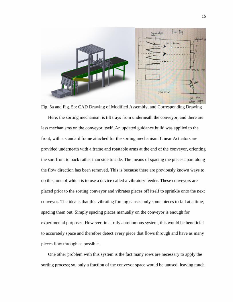
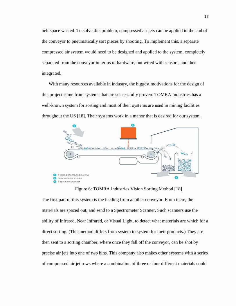
With many resources available in industry, the biggest motivations for the design of
this project came from systems that are successfully proven. TOMRA Industries has a
well-known system for sorting and most of their systems are used in mining facilities
throughout the US [18]. Their systems work in a manor that is desired for our system.
Figure 6: TOMRA Industries Vision Sorting Method [18]
The first part of this system is the feeding from another conveyor. From there, the
materials are spaced out, and send to a Spectrometer Scanner. Such scanners use the
ability of Infrared, Near Infrared, or Visual Light, to detect what materials are which for a
direct sorting. (This method differs from system to system for their products.) They are
then sent to a sorting chamber, where once they fall off the conveyor, can be shot by
precise air jets into one of two bins. This company also makes other systems with a series
of compressed air jet rows where a combination of three or four different materials could
18
be sorted out from one pile. For the first phase of this project, we will only implement
one row of air jets, for a simple two-material sort.
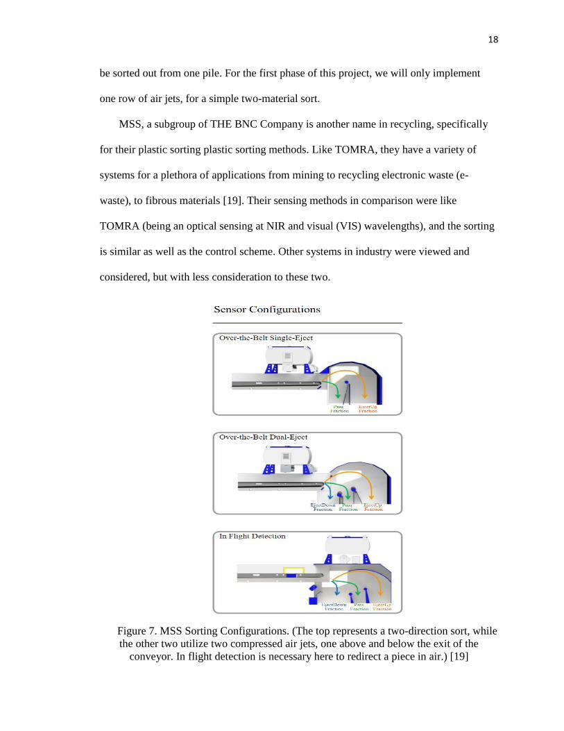
MSS, a subgroup of THE BNC Company is another name in recycling, specifically
for their plastic sorting plastic sorting methods. Like TOMRA, they have a variety of
systems for a plethora of applications from mining to recycling electronic waste (e-
waste), to fibrous materials [19]. Their sensing methods in comparison were like
TOMRA (being an optical sensing at NIR and visual (VIS) wavelengths), and the sorting
is similar as well as the control scheme. Other systems in industry were viewed and
considered, but with less consideration to these two.
Figure 7. MSS Sorting Configurations. (The top represents a two-direction sort, while
the other two utilize two compressed air jets, one above and below the exit of the
conveyor. In flight detection is necessary here to redirect a piece in air.) [19]
19
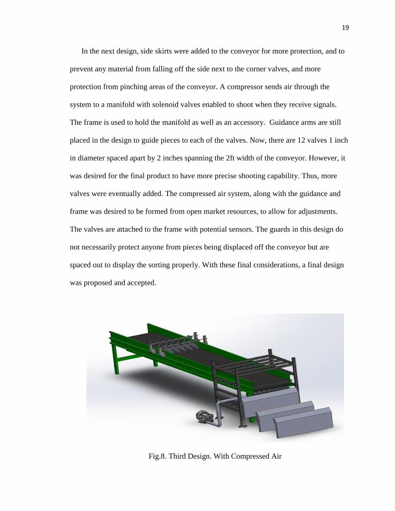
In the next design, side skirts were added to the conveyor for more protection, and to
prevent any material from falling off the side next to the corner valves, and more
protection from pinching areas of the conveyor. A compressor sends air through the
system to a manifold with solenoid valves enabled to shoot when they receive signals.
The frame is used to hold the manifold as well as an accessory. Guidance arms are still
placed in the design to guide pieces to each of the valves. Now, there are 12 valves 1 inch
in diameter spaced apart by 2 inches spanning the 2ft width of the conveyor. However, it
was desired for the final product to have more precise shooting capability. Thus, more
valves were eventually added. The compressed air system, along with the guidance and
frame was desired to be formed from open market resources, to allow for adjustments.
The valves are attached to the frame with potential sensors. The guards in this design do
not necessarily protect anyone from pieces being displaced off the conveyor but are
spaced out to display the sorting properly. With these final considerations, a final design
was proposed and accepted.
Fig.8. Third Design. With Compressed Air

20
1.3. Integrated Final Design
For the remainder of the work, this final approved design, which was slightly adjusted
during fabrication, represents the structural model of our system. The accessory frame
encompasses 50% of the conveyor length. This enables some space for the robot arm on
the side for other applications and gives space to load. A sorting chamber was placed at
the end where the compressed air system lays for added safety and has walls made from
sheet metal bolted to the frame. The ceiling uses sheets of polycarbonate material slightly
thicker than the aluminum to act as a more transparent solution and a potential spot for an
aerial view the system with a camera. These sheets are made transparent in Figure 9 to
show the interior compressed air system, which was made from open source CAD
drawings of the hardware being implemented [33, 34]. A case was added to this manifold
and designed to match the open source hardware drawings, so the manifold could be
mounted to the interior frame under the conveyor. A hose from the case attaches to the
compressor while the other end is sealed off. This manifold’s angle can be modified
manually, using an angled strut on the side of the interior frame which is attached
orthogonally to the manifold case. Some industrial systems use magnetic system to adjust
the angle, and so this angle adjustment feature was desired. Solenoid valves are used so
firing pieces can be achieved in a controlled fashion. The back of the frame has a brace
for more support when the air jets are on. The feet of the interior frame are 4ft long with
legs 2ft high to counterbalance the extra weight of the manifold components. Because of
the nature of the struts, it is possible to bolt anything to the frame such as sensors,
cameras or arms, which will overlook the conveyor for other applications.
21
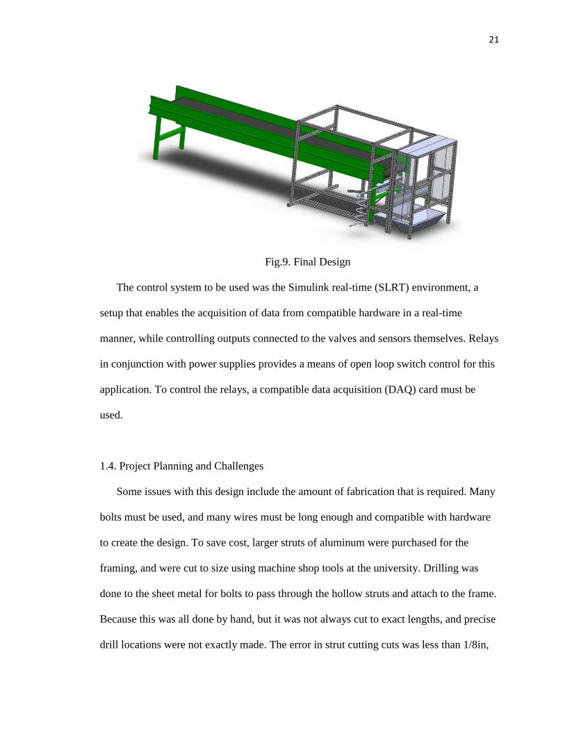
Fig.9. Final Design
The control system to be used was the Simulink real-time (SLRT) environment, a
setup that enables the acquisition of data from compatible hardware in a real-time
manner, while controlling outputs connected to the valves and sensors themselves. Relays
in conjunction with power supplies provides a means of open loop switch control for this
application. To control the relays, a compatible data acquisition (DAQ) card must be
used.
1.4. Project Planning and Challenges
Some issues with this design include the amount of fabrication that is required. Many
bolts must be used, and many wires must be long enough and compatible with hardware
to create the design. To save cost, larger struts of aluminum were purchased for the
framing, and were cut to size using machine shop tools at the university. Drilling was
done to the sheet metal for bolts to pass through the hollow struts and attach to the frame.
Because this was all done by hand, but it was not always cut to exact lengths, and precise
drill locations were not exactly made. The error in strut cutting cuts was less than 1/8in,
22
and the hole centers for drilling less than 1/4in. In the end however, the result was a set of
stable frames.
Incorporating this design into the lab space enabled us to have a conveyor for
recycling purposes. The design satisfies the goals of the project to shoot copper, and
aluminum, but also could be modified later to accurately sort them. Safety requirements
and considerations such as building codes were all satisfied. And the pieces can easily be
shot without fear of hitting anyone. While the design was thoroughly planned out at the
beginning, the implementation had to be troubleshooted frequently to ensure proper
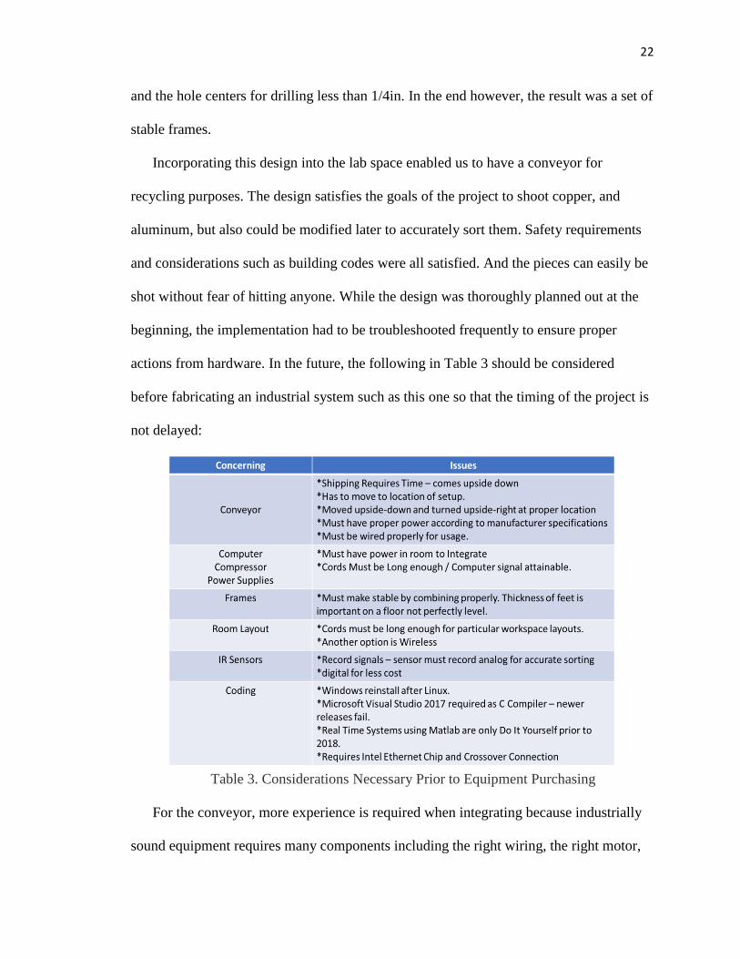
actions from hardware. In the future, the following in Table 3 should be considered
before fabricating an industrial system such as this one so that the timing of the project is
not delayed:
Table 3. Considerations Necessary Prior to Equipment Purchasing
For the conveyor, more experience is required when integrating because industrially
sound equipment requires many components including the right wiring, the right motor,
23
the right frame, the right assembly. and the right timing. Without the right timing with
shipping, receiving, moving equipment, and assembling the project is delayed. Each can
easily become an issue where some things are ready but other aren’t resulting in system
still not working, delaying testing to later dates.
There should always be a consideration of the workspace, including how many
devices are in use, what power supplies they have, and how separated they are from one
another. Because the layout of the space changed during fabrication time, it forced us to
order extra wires to connect pieces mounted at distances further away, move material
around slightly from the design, and use some wireless connectivity to operate the host
computer.
The hardware components are not the only problems that were faced. The software
can be incompatible at times. Because the robot arm works on Linux ROS system, and
SLRT works on Windows, it was necessary to program the host pc with both. On a first
trial, Linux USB boot caused us to lose the Windows Boot Manager. On a second trial,
Linux Boot was added to the Bios of the host PC to prevent this issue from occurring
again. Simulink real-time creates a variety of error codes when its C Compiler Microsoft
Visual Studio is not programmed correctly. Also, we determined the boot method for the
SLRT software can have some issues when trying to boot without certain pieces of
equipment.
24
2. Equipment, Fabrication, and Implementation
2.1 SJF Conveyor
2.1.1 Conveyor Specifications
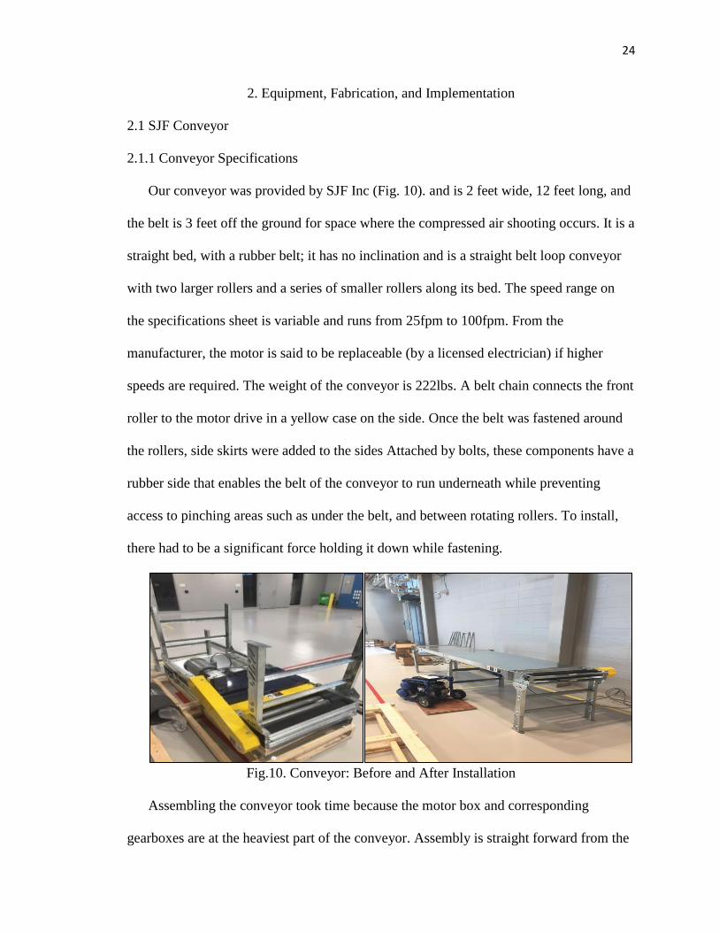
Our conveyor was provided by SJF Inc (Fig. 10). and is 2 feet wide, 12 feet long, and
the belt is 3 feet off the ground for space where the compressed air shooting occurs. It is a
straight bed, with a rubber belt; it has no inclination and is a straight belt loop conveyor
with two larger rollers and a series of smaller rollers along its bed. The speed range on
the specifications sheet is variable and runs from 25fpm to 100fpm. From the
manufacturer, the motor is said to be replaceable (by a licensed electrician) if higher
speeds are required. The weight of the conveyor is 222lbs. A belt chain connects the front
roller to the motor drive in a yellow case on the side. Once the belt was fastened around
the rollers, side skirts were added to the sides Attached by bolts, these components have a
rubber side that enables the belt of the conveyor to run underneath while preventing
access to pinching areas such as under the belt, and between rotating rollers. To install,
there had to be a significant force holding it down while fastening.
Fig.10. Conveyor: Before and After Installation
Assembling the conveyor took time because the motor box and corresponding
gearboxes are at the heaviest part of the conveyor. Assembly is straight forward from the
25
as the conveyors frame is simply metals bolted together. Once upright (the conveyor was
delivered upside-down), the legs could be spaced and bolted to create the entire frame.
Then, the feet of the conveyor can be leveled to the floor by the z-struts on each of 6 legs.
With the side skirts in contact with the belt constantly, this can create some drag relative
to the theoretical. The belt speed needed to be calibrated for timing the shots of the
compressed air precisely.
2.1.2. Motor Drive: Powerflex 520
The electrical components of the conveyor were supplied secondarily by Omni
Metal Craft. The motor is connected to the Power flex 520 AC Drive, which is mounted
to the back leg of the conveyor. From there the drive is connected to two emergencies
stop switches, and then the 480V room power. The 3-phase wiring was done and tested
by certified electricians. The motor in question had two voltage settings (230V, and
460V). For the motor to work properly, the wiring in the motor box must necessarily
match the High voltage configuration. If it does not, the driver stalls and the belt only run
for approximately one second and leads to an overload error.
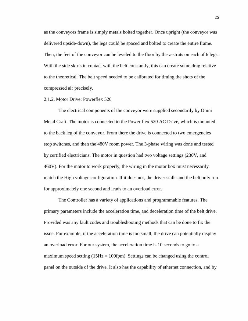
The Controller has a variety of applications and programmable features. The
primary parameters include the acceleration time, and deceleration time of the belt drive.
Provided was any fault codes and troubleshooting methods that can be done to fix the
issue. For example, if the acceleration time is too small, the drive can potentially display
an overload error. For our system, the acceleration time is 10 seconds to go to a
maximum speed setting (15Hz = 100fpm). Settings can be changed using the control
panel on the outside of the drive. It also has the capability of ethernet connection, and by
26
extension programming capability by the computer systems which could be added in the
future.
Fig.11. Settings and Control Panel for PLC
The lowest setting is 15Hz, and the highest is 60Hz. This corresponds to the belt
speed in a proportional relationship:
𝑣𝑏𝑒𝑙𝑡 =100𝑓𝑝𝑚
60𝐻𝑧 [𝑓] (2)
The control panel diagram in figure 11 describes the possible commands one can
give the drive. When implemented, it displays the frequency of the 3-phase motor with
which it is generating. To reverse the belt direction, press reverse (only after all is
stopped). The knob in the top right is the potentiometer, which adjusts the frequency, and
by extension, the effective current and conveyor speed. This PLC also has a reverse

27
button to change the direction of the conveyor flow. Starting and stopping the conveyor
can only be done through this panel manually.
2.1.3. Belt Installation
The belt itself is made from hard rubber and is cut specifically for the conveyor.
In other applications, there can be perforated belts made from plastics, which are more
applicable when dealing with food, but for metals, our belt suffices. The color is dark
grey, meaning anything other than that color will contrast with the belt as its being
delivered on the conveyor. Fastening the belt is as simple as holding both ends together
after it has been sent through the roller sections, and zipping with a metal wire through,
but tightening is done via the rollers near the rear end of the conveyor. A third roller for
belt tracking is directly under the conveyor near the motor box.
Tightening and tracking the belt is a timely process. Tightening the bolts on the
side translates each end of the roller toward the legs of the conveyor, thus tightening the
fit of the belt. This fit must be even though, and only orienting the belt correctly at one
end. On the other end, loosening and tightening the specified roller can adjust the flow of
the belt to the front roller. By running the belt for about an hour at moderate speed and
adjusting the tightness of the bolts, the belt can be tracked, and the belt will not be pulled
in either direction while running over a long period of time. It took two attempts to
properly track the belt on the rollers mainly due to the difficulty in accessing the front
roller with a frame underneath. The steps to tracking the belt are as follows:
1. Attach belt loosely on conveyor. Then tighten with bolts on rollers until the belt
can barely slide with manual force.
28
2. Start the conveyor: If belt slides to wall side, on back, tighten the wall side bolt. If
belt slides to the desk side, tighten the desk side bolt. Do this until belt is
relatively centered on back roller of conveyor.
3. If belt is sliding towards the wall on front roller, rotate roller underneath
conveyor towards room. If belt is sliding towards the room side, rotate slightly
towards the wall side.
4. If any part of the belt slips off the end of the conveyor, stop the conveyor, loosen
again and restart.
It is also important to clean the belt every so often as preventative maintenance.
Residue from metals, and room particles can cause unwanted weight distribution on the
belt, potentially leaning it side to side. So long as the belt stays relatively centered on the
conveyor, it can be used at any of its available speeds, indefinitely [20].
2.2 Framing components
2.2.1 Exterior Frame
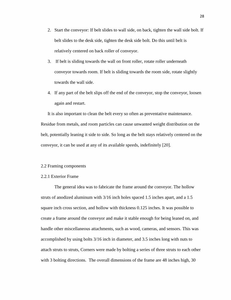
The general idea was to fabricate the frame around the conveyor. The hollow
struts of anodized aluminum with 3/16 inch holes spaced 1.5 inches apart, and a 1.5
square inch cross section, and hollow with thickness 0.125 inches. It was possible to
create a frame around the conveyor and make it stable enough for being leaned on, and
handle other miscellaneous attachments, such as wood, cameras, and sensors. This was
accomplished by using bolts 3/16 inch in diameter, and 3.5 inches long with nuts to
attach struts to struts, Corners were made by bolting a series of three struts to each other
with 3 bolting directions. The overall dimensions of the frame are 48 inches high, 30
29
inches wide, and 36 inches across. With 3 rows across above the conveyor for mounting
applications, which can be easily moved vertically, horizontally, added and subtracted for
various applications.
Fig. 12a, b. Final Exterior Frame, and Accessories [21].
The crisscross of the frame at its corners was formed because of the instability in the
frame in the CAD design. This instability existed because the frame was not stable
enough even with adjustable height legs. The cross section of the legs was not large
enough and rocking in the frame would occur even without significant loading.
Other framing struts and connections were considered such as T struts, and strut
channels. Both are sufficiently adjustable as well, but T-struts require more accessories,
and strut channels do not have uniform cross sections. Thus, these were not chosen as
options, but could be applied to the system for any future conveniences. Attachments like
the one shown in Figure 12, were purchased to provide extra options in framing and
connecting struts together. The exterior frame and interior frame only have a couple of
these, while the sorting chamber had many. These components, along with the struts were
purchased from McMaster and fabricated in the machine shop. One end is threaded while
30
the other is straight extrude, enabling struts to be bolted together while placed adjacent to
each other. This was very useful in fabricating the sorting chamber.
2.2.2. Sorting Chamber
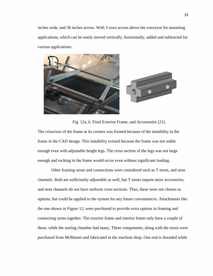
The sorting chamber is made from a combination of aluminum sheet metal,
polycarbonate sheets, that were drilled into and bolted to the frame. Polycarbonate was
considered because it is a plastic that has high impact resistance, and is more transparent
than aluminum sheets, potentially making sorting in the chamber more visual to the
outside [22]. For the final assembly, the aluminum sheets were chosen for the walls to
provide extra resistance, while the polycarbonate was used for the ceiling. Two cardboard
boxes were used for containers the metallic pieces could fall into, so they do not scatter
around the floor of the room. The reason the frame was built separate from the external
frame was to enable varying the distance of the threshold away from the end of the belt
conveyor, and to have easier access to pieces at the end of simulations as well. In the
front of the frame is one sheet of metal that acts as a barrier between the two sorted bins.
Figure 13. Sorting Chamber versus Design
2.3. Compressed Air Assembly
2.3.1. Interior Framing
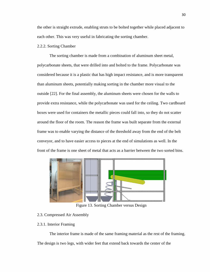
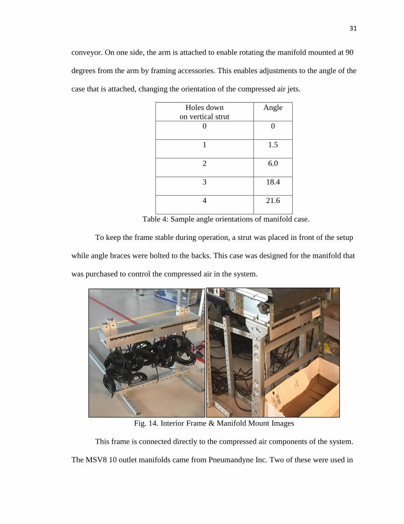
The interior frame is made of the same framing material as the rest of the framing.
The design is two legs, with wider feet that extend back towards the center of the
31
conveyor. On one side, the arm is attached to enable rotating the manifold mounted at 90
degrees from the arm by framing accessories. This enables adjustments to the angle of the
case that is attached, changing the orientation of the compressed air jets.
Holes down
on vertical strut
Angle
0 0
1 1.5
2 6.0
3 18.4
4 21.6
Table 4: Sample angle orientations of manifold case.
To keep the frame stable during operation, a strut was placed in front of the setup
while angle braces were bolted to the backs. This case was designed for the manifold that
was purchased to control the compressed air in the system.
Fig. 14. Interior Frame & Manifold Mount Images
This frame is connected directly to the compressed air components of the system.
The MSV8 10 outlet manifolds came from Pneumandyne Inc. Two of these were used in
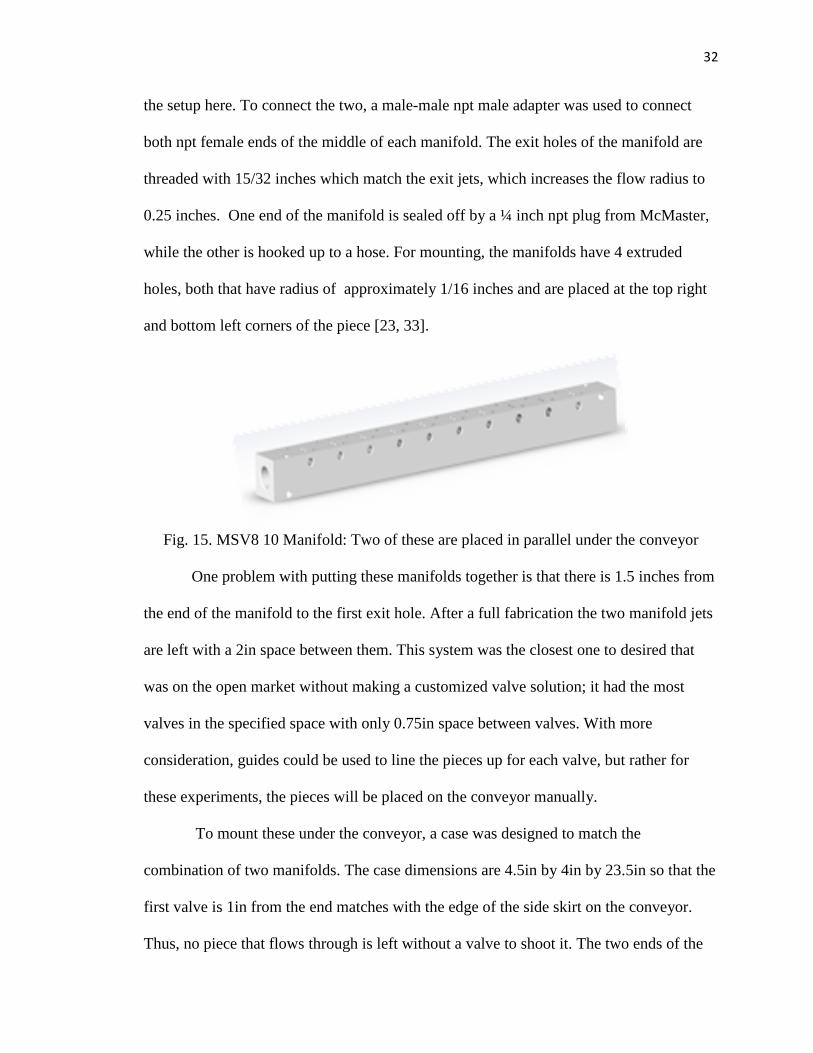
32
the setup here. To connect the two, a male-male npt male adapter was used to connect
both npt female ends of the middle of each manifold. The exit holes of the manifold are
threaded with 15/32 inches which match the exit jets, which increases the flow radius to
0.25 inches. One end of the manifold is sealed off by a ¼ inch npt plug from McMaster,
while the other is hooked up to a hose. For mounting, the manifolds have 4 extruded
holes, both that have radius of approximately 1/16 inches and are placed at the top right
and bottom left corners of the piece [23, 33].
Fig. 15. MSV8 10 Manifold: Two of these are placed in parallel under the conveyor
One problem with putting these manifolds together is that there is 1.5 inches from
the end of the manifold to the first exit hole. After a full fabrication the two manifold jets
are left with a 2in space between them. This system was the closest one to desired that
was on the open market without making a customized valve solution; it had the most
valves in the specified space with only 0.75in space between valves. With more
consideration, guides could be used to line the pieces up for each valve, but rather for
these experiments, the pieces will be placed on the conveyor manually.
To mount these under the conveyor, a case was designed to match the
combination of two manifolds. The case dimensions are 4.5in by 4in by 23.5in so that the
first valve is 1in from the end matches with the edge of the side skirt on the conveyor.
Thus, no piece that flows through is left without a valve to shoot it. The two ends of the
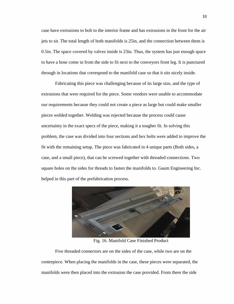
33
case have extrusions to bolt to the interior frame and has extrusions in the front for the air
jets to sit. The total length of both manifolds is 25in, and the connection between them is
0.5in. The space covered by valves inside is 23in. Thus, the system has just enough space
to have a hose come in from the side to fit next to the conveyors front leg. It is punctured
through in locations that correspond to the manifold case so that it sits nicely inside.
Fabricating this piece was challenging because of its large size, and the type of
extrusions that were required for the piece. Some vendors were unable to accommodate
our requirements because they could not create a piece as large but could make smaller
pieces welded together. Welding was rejected because the process could cause
uncertainty in the exact specs of the piece, making it a tougher fit. In solving this
problem, the case was divided into four sections and hex bolts were added to improve the
fit with the remaining setup. The piece was fabricated in 4 unique parts (Both sides, a
case, and a small piece), that can be screwed together with threaded connections. Two
square holes on the sides for threads to fasten the manifolds to. Gaum Engineering Inc.
helped in this part of the prefabrication process.
Fig. 16. Manifold Case Finished Product
Five threaded connectors are on the sides of the case, while two are on the
centerpiece. When placing the manifolds in the case, these pieces were separated, the
manifolds were then placed into the extrusion the case provided. From there the side
34
pieces were joined again, and then the bottom piece to firmly secure the case into the slot.
Finally, thin but long bolts were added to the small openings where the manifold case has
openings and sealed on the other end of the case.
It was beneficial to have the case designed with hex bolts because it was designed
with zero clearance for the manifold. If this was all made from one piece, it could have
required some modifications such as opening the extrusions slightly in the case where
welding would be required. With the bolts, the only issue in fabrication was the
extrusions were not exactly aligned from the sides to the piece (approximately 1/32in).
To solve this the pieces were individually attached, whereas the intent was to slip the
manifold through easily with little friction. The bolts are a stainless steel, and so have
some properties to be considered if any magnetic settings are added to the system in the
future.
2.3.2. Solenoid Valves and Jets
The solenoid valves and jets, like the manifolds, were from Pneumadyne. The jet
has a 0.25in quick connect which can be used with the hose for nearby robot arm. It also
has a 15/32 thread to connect to the manifold exits. Twenty of these were purchased, one
for each exit location on the manifold [23].
The S8 Solenoid valves are three-way valves that turn on with 12V signal and can
handle 0.5W of power. To mount them to the manifold they attach by two threads to the
top of every exit location, with a small rubber seal to prevent any leaks. The valves
operate such that air fires from the manifolds’ interior to the jet location when on, and air
moves out the top of the valve, and then exits the valve when turned off. This also keeps
the air from leaving the manifold. The valves have a response time of 10ms relative to a
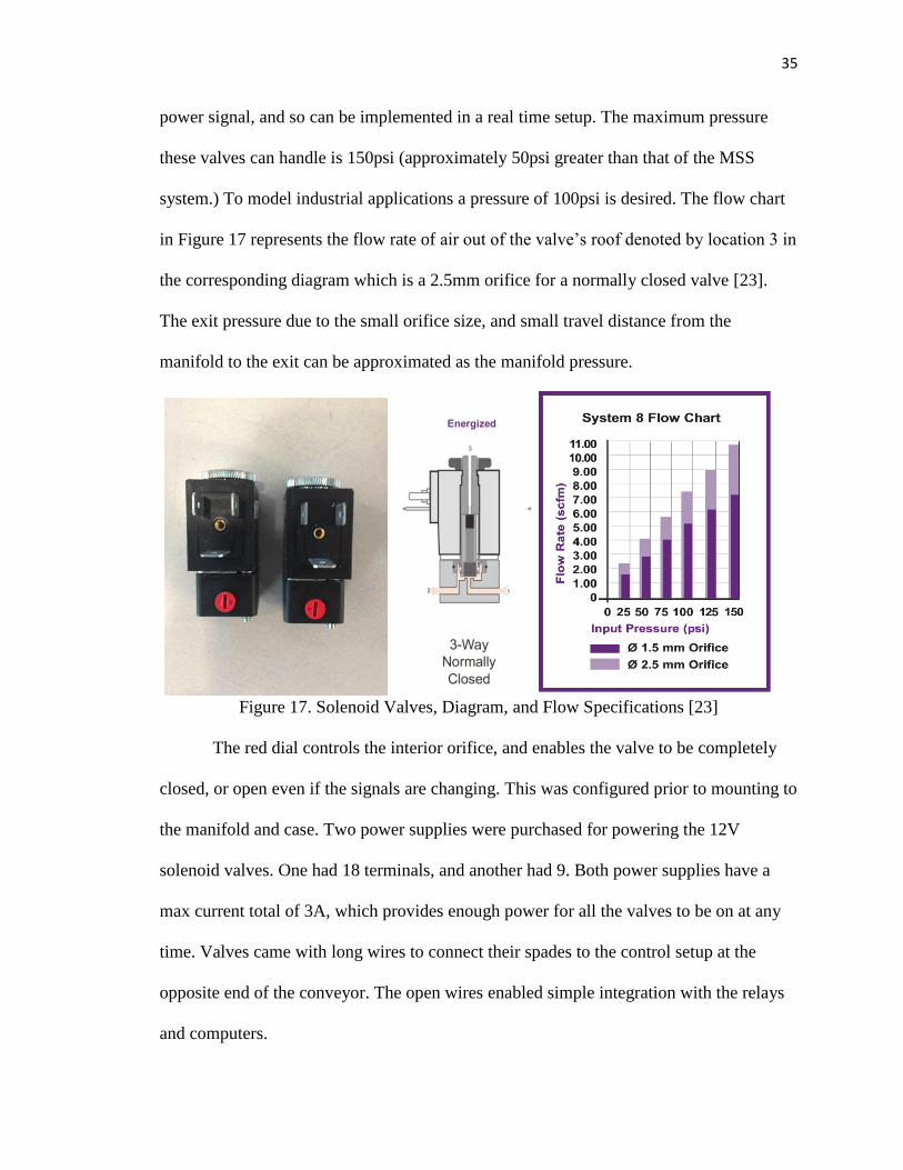
35
power signal, and so can be implemented in a real time setup. The maximum pressure
these valves can handle is 150psi (approximately 50psi greater than that of the MSS
system.) To model industrial applications a pressure of 100psi is desired. The flow chart
in Figure 17 represents the flow rate of air out of the valve’s roof denoted by location 3 in
the corresponding diagram which is a 2.5mm orifice for a normally closed valve [23].
The exit pressure due to the small orifice size, and small travel distance from the
manifold to the exit can be approximated as the manifold pressure.
Figure 17. Solenoid Valves, Diagram, and Flow Specifications [23]
The red dial controls the interior orifice, and enables the valve to be completely
closed, or open even if the signals are changing. This was configured prior to mounting to
the manifold and case. Two power supplies were purchased for powering the 12V
solenoid valves. One had 18 terminals, and another had 9. Both power supplies have a
max current total of 3A, which provides enough power for all the valves to be on at any
time. Valves came with long wires to connect their spades to the control setup at the
opposite end of the conveyor. The open wires enabled simple integration with the relays
and computers.

36
2.3.3. Power Supplies and Eagle EA 5000 Compressor
To shoot small pieces of copper, about 1in3, the force required to push a piece
over a barrier height of 1 ft (about 14-16in below the jets) must be supplied by the air
jets. The density of a piece of copper is approximately 8.96g/cm3 (0.324 lb./in3), and
2.70g/cm3 (0.098lb/in3) for aluminum. Having the manifold at an angle, with a height of
approximately 2.5ft from the ground (0.5ft from the top of the belt), and a shooting angle
of approximately 6 degrees, a model could be made for determining minimum pressure to
create a force through a valve with a diameter of 0.25in using elementary kinematics.
This simulation is not effective because it is difficult to account for air resistance (drag
coefficients) given the variable orientation of each piece, and its effective area hit by the
piece, the impact time, how far pieces are from the jet when in free fall, and the rotation
involved in the particle dynamics, as well as the trajectory off the desired path which is
straight out from the jets. Due to these uncertain variables, a variable pressure setting was
desired for which to do some testing.
The compressor chosen for this task is the Eagle 5000 Air compressor (Figure
18), because it has the capability to use a standard 120V outlet for power, has wheels to
move around for added design flexibility, uses a 2HP motor to pump air in, and has a
max pressure of 125psi. Inside is a regulator which enables pressure settings at any
pressure under the maximum. As an added measure, if the pressure in the storage tank
falls below 90psi, the compressor automatically turns on again. The exhaust port of this
compressor is a 0.25in quick connect. To connect this to the manifold case, a hose with
one end with a quick connect nose, and another with a npt male thread is used. The
mobility in the compressor was also a bonus to this setup, making adjustments easier.
37
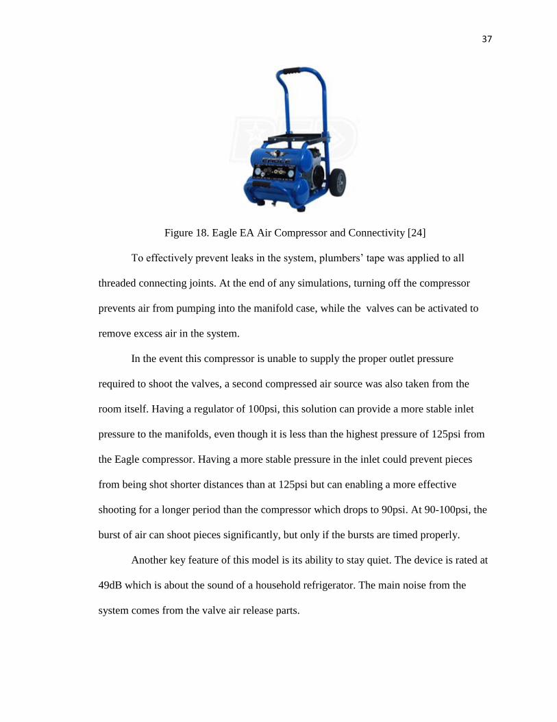
Figure 18. Eagle EA Air Compressor and Connectivity [24]
To effectively prevent leaks in the system, plumbers’ tape was applied to all
threaded connecting joints. At the end of any simulations, turning off the compressor
prevents air from pumping into the manifold case, while the valves can be activated to
remove excess air in the system.
In the event this compressor is unable to supply the proper outlet pressure
required to shoot the valves, a second compressed air source was also taken from the
room itself. Having a regulator of 100psi, this solution can provide a more stable inlet
pressure to the manifolds, even though it is less than the highest pressure of 125psi from
the Eagle compressor. Having a more stable pressure in the inlet could prevent pieces
from being shot shorter distances than at 125psi but can enabling a more effective
shooting for a longer period than the compressor which drops to 90psi. At 90-100psi, the
burst of air can shoot pieces significantly, but only if the bursts are timed properly.
Another key feature of this model is its ability to stay quiet. The device is rated at
49dB which is about the sound of a household refrigerator. The main noise from the
system comes from the valve air release parts.
38
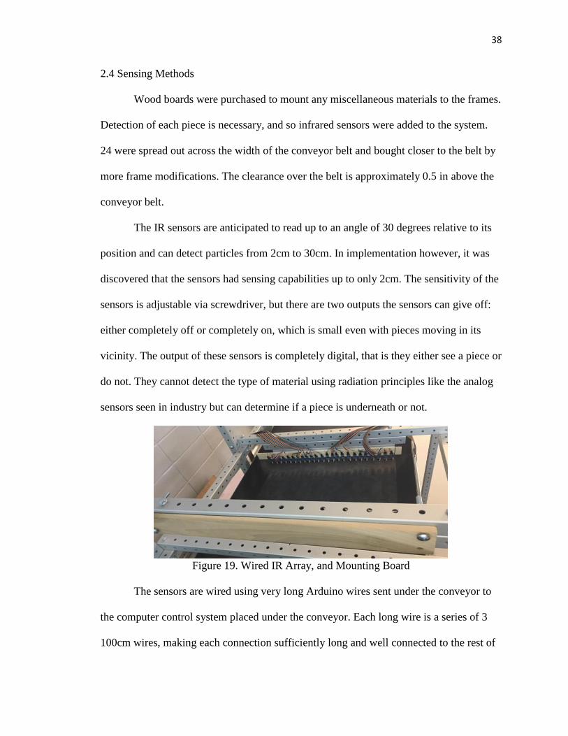
2.4 Sensing Methods
Wood boards were purchased to mount any miscellaneous materials to the frames.
Detection of each piece is necessary, and so infrared sensors were added to the system.
24 were spread out across the width of the conveyor belt and bought closer to the belt by
more frame modifications. The clearance over the belt is approximately 0.5 in above the
conveyor belt.
The IR sensors are anticipated to read up to an angle of 30 degrees relative to its
position and can detect particles from 2cm to 30cm. In implementation however, it was
discovered that the sensors had sensing capabilities up to only 2cm. The sensitivity of the
sensors is adjustable via screwdriver, but there are two outputs the sensors can give off:
either completely off or completely on, which is small even with pieces moving in its
vicinity. The output of these sensors is completely digital, that is they either see a piece or
do not. They cannot detect the type of material using radiation principles like the analog
sensors seen in industry but can determine if a piece is underneath or not.
Figure 19. Wired IR Array, and Mounting Board
The sensors are wired using very long Arduino wires sent under the conveyor to
the computer control system placed under the conveyor. Each long wire is a series of 3
100cm wires, making each connection sufficiently long and well connected to the rest of
39
the controls. With their digital inputs, the pieces can be identified and shot, but will only
be indirectly sorted [9]. Whereas the pieces can’t be sorted by material, they can
potentially be sorted by size, and by color where larger pieces can be recorded and shot,
while the smaller ones are not.
2.5 Control Scheme Hardware
2.5.1 5V Relay Modules and Dell Optiplex 3060
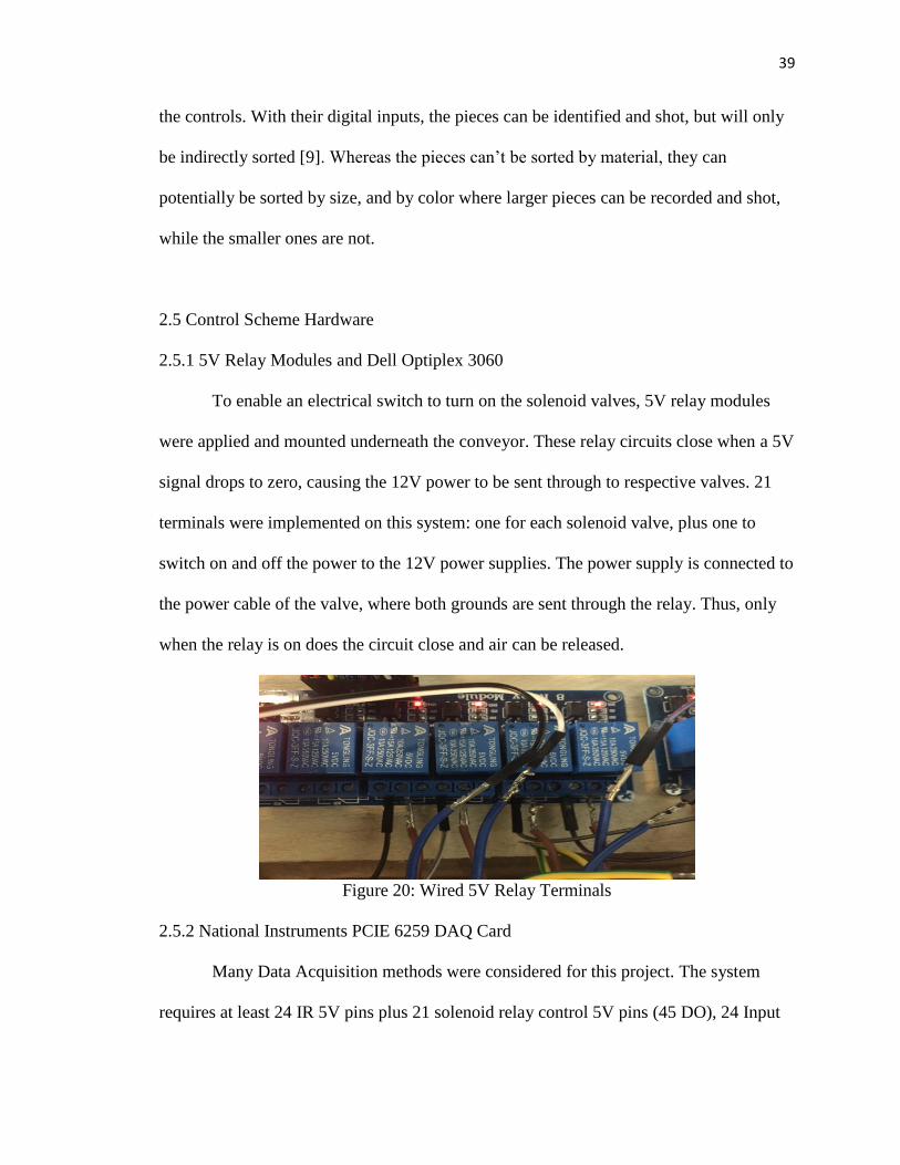
To enable an electrical switch to turn on the solenoid valves, 5V relay modules
were applied and mounted underneath the conveyor. These relay circuits close when a 5V
signal drops to zero, causing the 12V power to be sent through to respective valves. 21
terminals were implemented on this system: one for each solenoid valve, plus one to
switch on and off the power to the 12V power supplies. The power supply is connected to
the power cable of the valve, where both grounds are sent through the relay. Thus, only
when the relay is on does the circuit close and air can be released.
Figure 20: Wired 5V Relay Terminals
2.5.2 National Instruments PCIE 6259 DAQ Card
Many Data Acquisition methods were considered for this project. The system
requires at least 24 IR 5V pins plus 21 solenoid relay control 5V pins (45 DO), 24 Input
40
Pins, and a simple configuration for implementation. Because MATLAB-Simulink was
the desired method of control, the hardware necessarily had to be compatible with it [26].
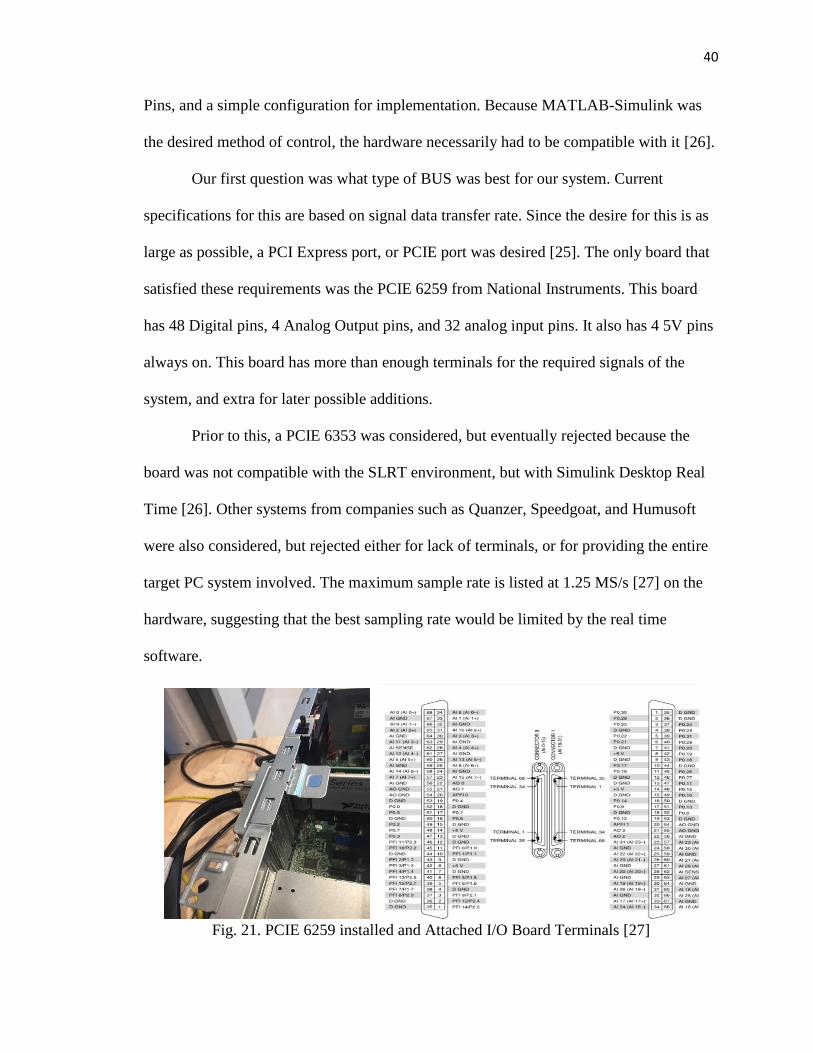
Our first question was what type of BUS was best for our system. Current
specifications for this are based on signal data transfer rate. Since the desire for this is as
large as possible, a PCI Express port, or PCIE port was desired [25]. The only board that
satisfied these requirements was the PCIE 6259 from National Instruments. This board
has 48 Digital pins, 4 Analog Output pins, and 32 analog input pins. It also has 4 5V pins
always on. This board has more than enough terminals for the required signals of the
system, and extra for later possible additions.
Prior to this, a PCIE 6353 was considered, but eventually rejected because the
board was not compatible with the SLRT environment, but with Simulink Desktop Real
Time [26]. Other systems from companies such as Quanzer, Speedgoat, and Humusoft
were also considered, but rejected either for lack of terminals, or for providing the entire
target PC system involved. The maximum sample rate is listed at 1.25 MS/s [27] on the
hardware, suggesting that the best sampling rate would be limited by the real time
software.
Fig. 21. PCIE 6259 installed and Attached I/O Board Terminals [27]
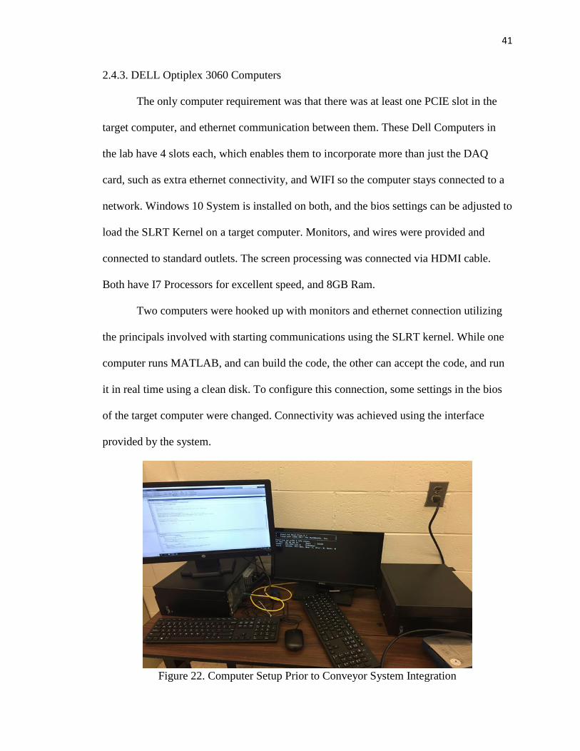
41
2.4.3. DELL Optiplex 3060 Computers
The only computer requirement was that there was at least one PCIE slot in the
target computer, and ethernet communication between them. These Dell Computers in
the lab have 4 slots each, which enables them to incorporate more than just the DAQ
card, such as extra ethernet connectivity, and WIFI so the computer stays connected to a
network. Windows 10 System is installed on both, and the bios settings can be adjusted to
load the SLRT Kernel on a target computer. Monitors, and wires were provided and
connected to standard outlets. The screen processing was connected via HDMI cable.
Both have I7 Processors for excellent speed, and 8GB Ram.
Two computers were hooked up with monitors and ethernet connection utilizing
the principals involved with starting communications using the SLRT kernel. While one
computer runs MATLAB, and can build the code, the other can accept the code, and run
it in real time using a clean disk. To configure this connection, some settings in the bios
of the target computer were changed. Connectivity was achieved using the interface
provided by the system.
Figure 22. Computer Setup Prior to Conveyor System Integration
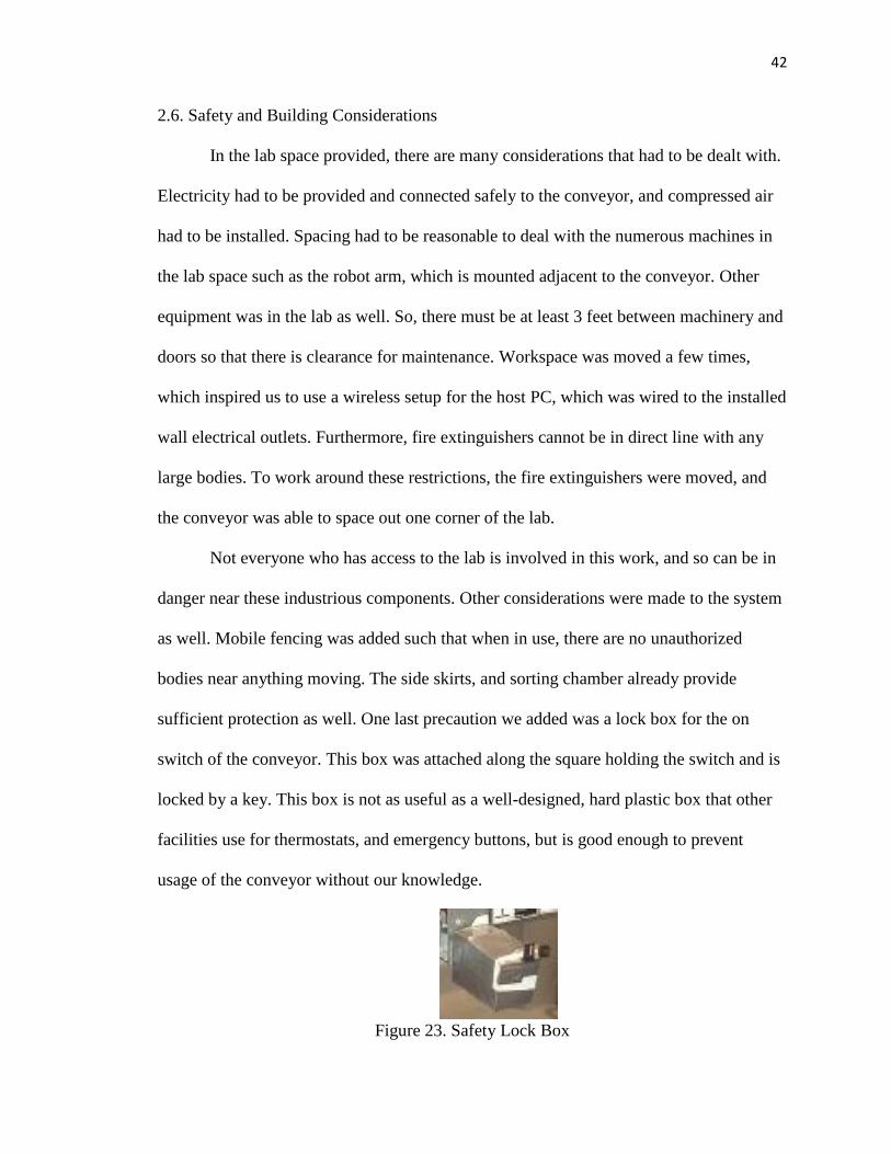
42
2.6. Safety and Building Considerations
In the lab space provided, there are many considerations that had to be dealt with.
Electricity had to be provided and connected safely to the conveyor, and compressed air
had to be installed. Spacing had to be reasonable to deal with the numerous machines in
the lab space such as the robot arm, which is mounted adjacent to the conveyor. Other
equipment was in the lab as well. So, there must be at least 3 feet between machinery and
doors so that there is clearance for maintenance. Workspace was moved a few times,
which inspired us to use a wireless setup for the host PC, which was wired to the installed
wall electrical outlets. Furthermore, fire extinguishers cannot be in direct line with any
large bodies. To work around these restrictions, the fire extinguishers were moved, and
the conveyor was able to space out one corner of the lab.
Not everyone who has access to the lab is involved in this work, and so can be in
danger near these industrious components. Other considerations were made to the system
as well. Mobile fencing was added such that when in use, there are no unauthorized
bodies near anything moving. The side skirts, and sorting chamber already provide
sufficient protection as well. One last precaution we added was a lock box for the on
switch of the conveyor. This box was attached along the square holding the switch and is
locked by a key. This box is not as useful as a well-designed, hard plastic box that other
facilities use for thermostats, and emergency buttons, but is good enough to prevent
usage of the conveyor without our knowledge.
Figure 23. Safety Lock Box
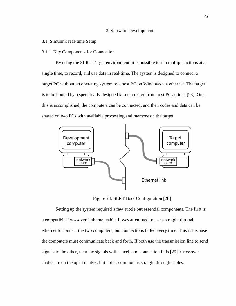
43
3. Software Development
3.1. Simulink real-time Setup
3.1.1. Key Components for Connection
By using the SLRT Target environment, it is possible to run multiple actions at a
single time, to record, and use data in real-time. The system is designed to connect a
target PC without an operating system to a host PC on Windows via ethernet. The target
is to be booted by a specifically designed kernel created from host PC actions [28]. Once
this is accomplished, the computers can be connected, and then codes and data can be
shared on two PCs with available processing and memory on the target.
Figure 24: SLRT Boot Configuration [28]
Setting up the system required a few subtle but essential components. The first is
a compatible “crossover” ethernet cable. It was attempted to use a straight through
ethernet to connect the two computers, but connections failed every time. This is because
the computers must communicate back and forth. If both use the transmission line to send
signals to the other, then the signals will cancel, and connection fails [29]. Crossover
cables are on the open market, but not as common as straight through cables.

44
The next requirement is the network cards on the host and target PCs for which
the ethernet connection is established. Because the Optiplex computers come with a
Realtek ethernet card, the connection with the SLRT kernel will not be successful
because it is not a verified network card for this application. To work-around for this, a
proper card in either the host or target computer must be installed; both configurations are
satisfactory. The card chosen to replace the Realtek card was the Intel I8254x card which
connects to the host PC in another PCIE slot [30]. To upload the kernel to the target PC
there are a variety of boot methods. The simplest is network boot, where the system is
booted through the ethernet, from a removable drive or CD, a standalone boot, where the
code is preprogrammed on the target and doesn’t need the host, or a DOS loader. The
first attempt was by network boot, but no connectivity was found. Using the removable
drive method with a bootable partition enabled us to have a disk drive where the SLRT
would boot from.
Configuring the system parameters is the final step in the setup. A built-in
interface is used in this process by entering codes in the command window. From there, it
is possible to assign an IP address, Subnet Mask and Gateway to the Target PC, and then
connect to it using the host PC control panel. To do this correctly, only the IPV4 setting
on the ethernet connection must be on. All other settings should be off, or the host will
try other methods to connect with the target, causing the connection to ultimately fail. If
the settings on the host, and target are compatible, then the connection is made, and the
setup is complete. Testing of this was done using built in codes and graphical interfaces
provided by MATLAB-Simulink. In the bios of the target PC, the boot order was

45
changed to boot from removable disk. This was configured by unselecting secure boot,
finding the properly set up USB in the PC and skipping Windows Boot Manager.
The SLRT environment also requires a C Compiler for which code can be
transferred between host and target. The most compatible system for this is Microsoft
Visual Studio 2017. Proper settings for this installation were also required. If these
settings are not accounted for, then errors will be found while building a code onto the
target PC [31]. The specific requirements include Windows 10 SDK 10.0.14393.0, and
VC ++ 2017 Toolset. These are used when building codes to a target PC, and so must be
configured in the Visual Studio Installation.
3.1.2. Calibration of DAQ Card to Simulink Blocks
Blocks that allow for control of the DAQ card can be applied to Simulink models
prior to 2018. As of 2014 MathWorks began supporting Speedgoat Target Computers as
their primary target computers, and completely lost support for Do It Yourself Targets
(DIY) by this time. Thus, the MATLAB year of choice for this project had to be R2017b.
Furthermore, the blocks with the DAQ card were listed under a dialog “xpcobsoletelib”
because the DAQ card system is considered obsolete. In any event, the system has
everything it needs to be applied to the DAQ card attached to the target PC.
There are 9 blocks that can possibly be used for the DAQ Card. There is one
block for Analog Output (AO), One for Analog Input (AI), One for Digital Input and
Output (DI/O), PFI DI/O, and four others which are unused for this application. There are
4 AO pins possible, 32 AI pins, 32 DI/O pins and 16 PFI DI/O pins which adds up to the
totals in the specification’s manual. However, the digital pins on the DAQ card, and the
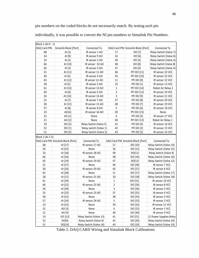
46
pin numbers on the coded blocks do not necessarily match. By testing each pin
individually, it was possible to convert the NI pin numbers to Simulink Pin Numbers.
Table 5. DAQ CARD Wiring and Simulink Block Calibrations
Block 1 (AI 0 - 1)
DAQ Card PIN Simulink Block [Port] Connected To DAQ Card PIN Simulink Block [Port] Connected To
68 AI [1] IR sensor 1 AO 17 DO [7] Relay Switch (Valve 7)
34 AI [9] IR sensor 9 AO 16 DO [6] Relay Switch (Valve 6)
33 AI [2] IR sensor 2 AO 49 DO [3] Relay Swtich (Valve 3)
66 AI [10] IR sensor 10 AO 48 DO [8] Relay Swtich (Valve 8)
65 AI [3] IR sensor 3 AO 47 DO [4] Relay Switch (Valve 4)
31 AI [11] IR sensor 11 AO 46 PFI DO [11] IR sensor 23 VCC
30 AI [4] IR sensor 4 AO 45 PFI DO [10] IR sensor 22 VCC
63 AI [12] IR sensor 12 AO 11 PFI DO [0] IR sensor 12 VCC
28 AI [5] IR sensor 5 AO 10 PFI DO [1] IR sensor 13 VCC
61 AI [13] IR sensor 13 AO 1 PFI DO [14] Robot Air Relay 2
60 AI [6] IR sensor 6 AO 2 PFI DO [12] IR sensor 24 VCC
26 AI [14] IR sensor 14 AO 3 PFI DO [9] IR sensor 21 VCC
25 AI [7] IR sensor 7 AO 37 PFI DO [8] IR sensor 20 VCC
58 AI [15] IR sensor 15 AO 38 PFI DO [7] IR sensor 19 VCC
57 AI [8] IR sensor 8 AO 5 PFI DO [6] IR sensor 18 VCC
23 AI[16] IR sensor 16 AO 39 PFI DO [15] None
22 AO [1] None 6 PFI DO [5] IR sensor 17 VCC
21 AO [2] None 40 PFI DO [13] Robot Air Relay 1
19 DO [5] Relay Switch (Valve 5) 41 PFI DO [4] IR sensor 16 VCC
52 DO [1] Relay switch (Valve 1) 42 PFI DO [3] IR sensor 15 VCC
51 DO [2] Relay Switch (Valve 2) 43 PFI DO [2] IR sensor 14 VCC
Block 2 (AI 2-3)
DAQ Card PIN Simulink Block [Port] Connected To DAQ Card PIN Simulink Block [Port] Connected To
68 AI [17] IR sensor 17 AO 17 DO [10] Relay Swtich (Valve 10)
34 AI [25] None 16 DO [15] Relay Swtich (Valve 15)
33 AI [18] IR sensor 18 AO 49 DO[11] Relay Swtich (Valve 9)
66 AI [26] None 48 DO [16] Relay Swtich (Valve 16)
65 AI [19] IR sensor 19 AO 47 DO[12] Relay Swtich (Valve 12)
31 AI [27] None 46 DO [28] IR sensor 7 VCC
30 AI [20] IR sensor 20 AO 45 DO [27] IR sensor 6 VCC
63 AI [28] None 11 DO [17] Relay Swtich (Valve 17)
28 AI [21] IR sensor 21 AO 10 DO [18] Relay Swtich (Valve 18)
61 AI [29] None 1 DO [31] IR sensor 10 VCC
60 AI [22] IR sensor 22 AO 2 DO [29] IR sensor 8 VCC
26 AI [30] None 3 DO [26] IR sensor 5 VCC
25 AI [23] IR sensor 23 AO 37 DO [25] IR sensor 4 VCC
58 AI [31] None 38 DO [24] IR sensor 3 VCC
57 AI [24] IR sensor 24 AO 5 DO [23] IR sensor 2 VCC
23 AI [32] None 39 DO [32] IR sensor 11 VCC
22 AO [3] None 6 DO [22] IR sensor 1 VCC
21 AO [4] None 40 DO [30] IR sensor 9 VCC
19 DO [13] Relay Swtich (Valve 13) 41 DO [21] 12 Power Supplies Relay
52 DO[9] Relay Swtich (Valve 9) 42 DO [20] Relay Swtich (Valve 20)
51 DO[14] Relay Swtich (Valve 14) 43 DO [19] Relay Swtich (Valve 19)
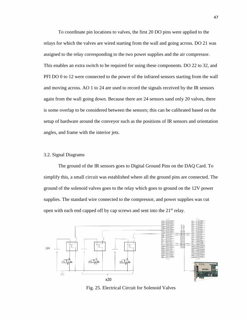
47
To coordinate pin locations to valves, the first 20 DO pins were applied to the
relays for which the valves are wired starting from the wall and going across. DO 21 was
assigned to the relay corresponding to the two power supplies and the air compressor.
This enables an extra switch to be required for using these components. DO 22 to 32, and
PFI DO 0 to 12 were connected to the power of the infrared sensors starting from the wall
and moving across. AO 1 to 24 are used to record the signals received by the IR sensors
again from the wall going down. Because there are 24 sensors sand only 20 valves, there
is some overlap to be considered between the sensors; this can be calibrated based on the
setup of hardware around the conveyor such as the positions of IR sensors and orientation
angles, and frame with the interior jets.
3.2. Signal Diagrams
The ground of the IR sensors goes to Digital Ground Pins on the DAQ Card. To
simplify this, a small circuit was established where all the ground pins are connected. The
ground of the solenoid valves goes to the relay which goes to ground on the 12V power
supplies. The standard wire connected to the compressor, and power supplies was cut
open with each end capped off by cap screws and sent into the 21st relay.
Fig. 25. Electrical Circuit for Solenoid Valves
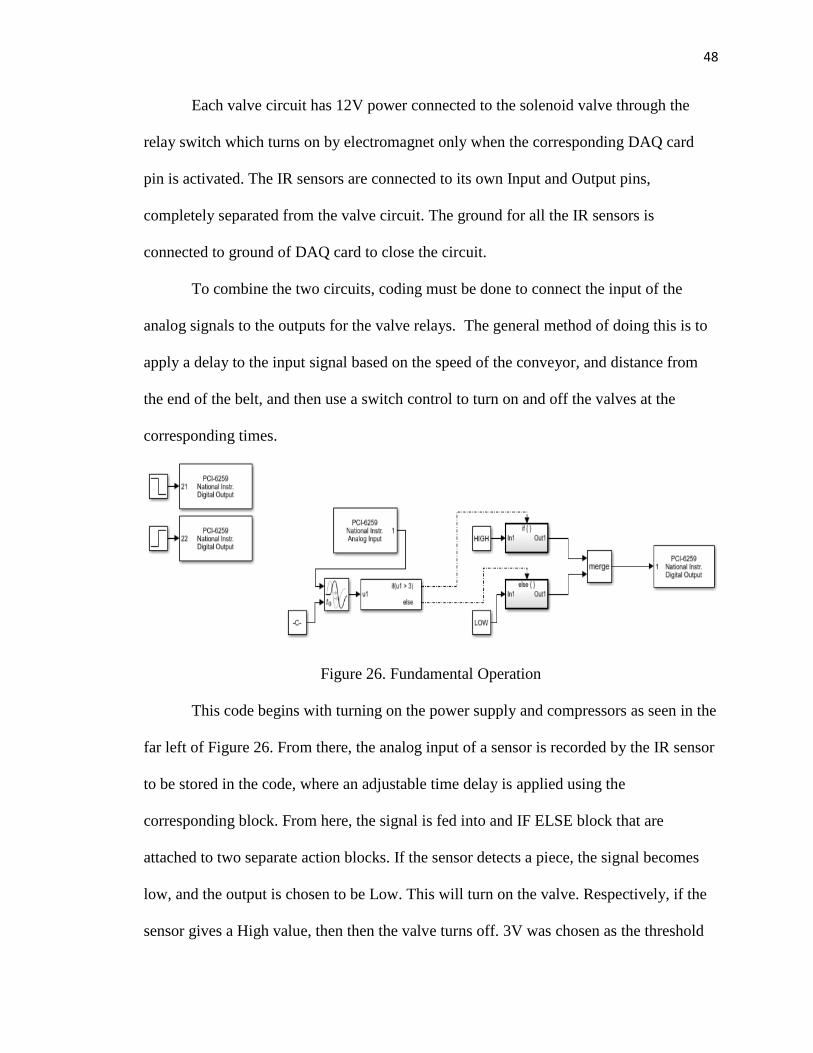
48
Each valve circuit has 12V power connected to the solenoid valve through the
relay switch which turns on by electromagnet only when the corresponding DAQ card
pin is activated. The IR sensors are connected to its own Input and Output pins,
completely separated from the valve circuit. The ground for all the IR sensors is
connected to ground of DAQ card to close the circuit.
To combine the two circuits, coding must be done to connect the input of the
analog signals to the outputs for the valve relays. The general method of doing this is to
apply a delay to the input signal based on the speed of the conveyor, and distance from
the end of the belt, and then use a switch control to turn on and off the valves at the
corresponding times.
Figure 26. Fundamental Operation
This code begins with turning on the power supply and compressors as seen in the
far left of Figure 26. From there, the analog input of a sensor is recorded by the IR sensor
to be stored in the code, where an adjustable time delay is applied using the
corresponding block. From here, the signal is fed into and IF ELSE block that are
attached to two separate action blocks. If the sensor detects a piece, the signal becomes
low, and the output is chosen to be Low. This will turn on the valve. Respectively, if the
sensor gives a High value, then then the valve turns off. 3V was chosen as the threshold
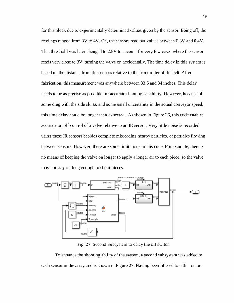
49
for this block due to experimentally determined values given by the sensor. Being off, the
readings ranged from 3V to 4V. On, the sensors read out values between 0.3V and 0.4V.
This threshold was later changed to 2.5V to account for very few cases where the sensor
reads very close to 3V, turning the valve on accidentally. The time delay in this system is
based on the distance from the sensors relative to the front roller of the belt. After
fabrication, this measurement was anywhere between 33.5 and 34 inches. This delay
needs to be as precise as possible for accurate shooting capability. However, because of
some drag with the side skirts, and some small uncertainty in the actual conveyor speed,
this time delay could be longer than expected. As shown in Figure 26, this code enables
accurate on off control of a valve relative to an IR sensor. Very little noise is recorded
using these IR sensors besides complete misreading nearby particles, or particles flowing
between sensors. However, there are some limitations in this code. For example, there is
no means of keeping the valve on longer to apply a longer air to each piece, so the valve
may not stay on long enough to shoot pieces.
Fig. 27. Second Subsystem to delay the off switch.
To enhance the shooting ability of the system, a second subsystem was added to
each sensor in the array and is shown in Figure 27. Having been filtered to either on or
50
off based on piece flow, it was possible to delay the turn-off time of the valves to when a
piece was no longer near falling off the conveyor. This was done by looking at the sign
of the derivative of the filtered sensor signal. When a signal is being turned on, the
derivative has a negative value. If negative, these blocks are designed to output 0 to turn
on the relays. If not, then the signal takes on a value of 5, but only if the system has no
memory of being turned on. If the signal is on, the function uses the memory of the
diagrams previous output, holding the signal as it was. During this time, a counter is
implemented and runs at the sample time of the whole block diagram. When the counter
reaches the step time, the output switches to off at 5V. The output of this code is then on
when the signal is turned on or held on, and then remains on until the counter starts by
checking if the derivative of the input is positive. If the signal becomes negative again
before the timer goes off, then the signal remains on until the last time the pieces were
not found, depicted by an increase in the signal (positive derivative), and the time delay
was considered.
Demonstrations of this code were tested using a variety of square input signals
and then modified for the actual inputs of the IR sensors. For the shoot time, a short time
is enough because the pieces are in in air for only less than half a second. However, this
time should be at least longer than the sample time of the system to have any benefits at
all.
3.3. Control Scheme
From start to Finish, the block diagram begins with power to the power supplies, and
IR sensors. A step signals up to 5V was sent to each IR sensor to power them as well as
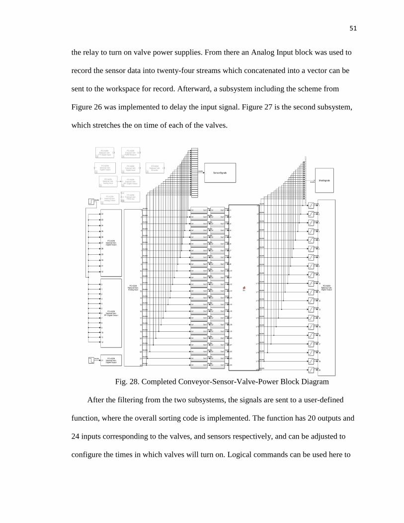
51
the relay to turn on valve power supplies. From there an Analog Input block was used to
record the sensor data into twenty-four streams which concatenated into a vector can be
sent to the workspace for record. Afterward, a subsystem including the scheme from
Figure 26 was implemented to delay the input signal. Figure 27 is the second subsystem,
which stretches the on time of each of the valves.
Fig. 28. Completed Conveyor-Sensor-Valve-Power Block Diagram
After the filtering from the two subsystems, the signals are sent to a user-defined
function, where the overall sorting code is implemented. The function has 20 outputs and
24 inputs corresponding to the valves, and sensors respectively, and can be adjusted to
configure the times in which valves will turn on. Logical commands can be used here to
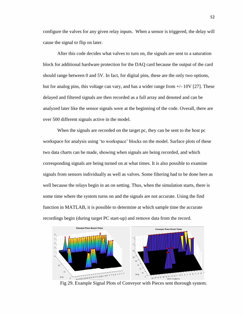
52
configure the valves for any given relay inputs. When a sensor is triggered, the delay will
cause the signal to flip on later.
After this code decides what valves to turn on, the signals are sent to a saturation
block for additional hardware protection for the DAQ card because the output of the card
should range between 0 and 5V. In fact, for digital pins, these are the only two options,
but for analog pins, this voltage can vary, and has a wider range from +/- 10V [27]. These
delayed and filtered signals are then recorded as a full array and denoted and can be
analyzed later like the sensor signals were at the beginning of the code. Overall, there are
over 500 different signals active in the model.
When the signals are recorded on the target pc, they can be sent to the host pc
workspace for analysis using ‘to workspace’ blocks on the model. Surface plots of these
two data charts can be made, showing when signals are being recorded, and which
corresponding signals are being turned on at what times. It is also possible to examine
signals from sensors individually as well as valves. Some filtering had to be done here as
well because the relays begin in an on setting. Thus, when the simulation starts, there is
some time where the system turns on and the signals are not accurate. Using the find
function in MATLAB, it is possible to determine at which sample time the accurate
recordings begin (during target PC start-up) and remove data from the record.
Fig 29. Example Signal Plots of Conveyor with Pieces sent thorough system.
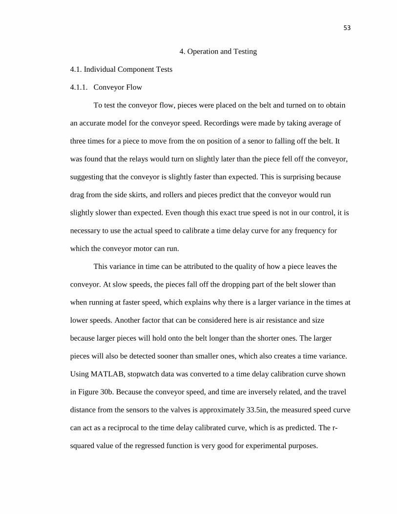
53
4. Operation and Testing
4.1. Individual Component Tests
4.1.1. Conveyor Flow
To test the conveyor flow, pieces were placed on the belt and turned on to obtain
an accurate model for the conveyor speed. Recordings were made by taking average of
three times for a piece to move from the on position of a senor to falling off the belt. It
was found that the relays would turn on slightly later than the piece fell off the conveyor,
suggesting that the conveyor is slightly faster than expected. This is surprising because
drag from the side skirts, and rollers and pieces predict that the conveyor would run
slightly slower than expected. Even though this exact true speed is not in our control, it is
necessary to use the actual speed to calibrate a time delay curve for any frequency for
which the conveyor motor can run.
This variance in time can be attributed to the quality of how a piece leaves the
conveyor. At slow speeds, the pieces fall off the dropping part of the belt slower than
when running at faster speed, which explains why there is a larger variance in the times at
lower speeds. Another factor that can be considered here is air resistance and size
because larger pieces will hold onto the belt longer than the shorter ones. The larger
pieces will also be detected sooner than smaller ones, which also creates a time variance.
Using MATLAB, stopwatch data was converted to a time delay calibration curve shown
in Figure 30b. Because the conveyor speed, and time are inversely related, and the travel
distance from the sensors to the valves is approximately 33.5in, the measured speed curve
can act as a reciprocal to the time delay calibrated curve, which is as predicted. The r-
squared value of the regressed function is very good for experimental purposes.
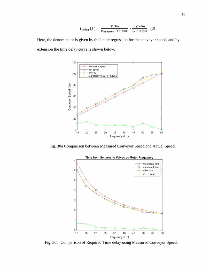
54
𝑡𝑑𝑒𝑙𝑎𝑦(𝑓) =33.5𝑖𝑛
𝑣𝑚𝑒𝑎𝑠𝑢𝑟𝑒𝑑(𝑓) (𝑓𝑝𝑛)∗
1𝑓𝑡∗60𝑠
12𝑖𝑛∗1𝑚𝑖𝑛 (3)
Here, the denominator is given by the linear regression for the conveyor speed, and by
extension the time delay curve is shown below.
Fig. 30a Comparison between Measured Conveyor Speed and Actual Speed.
Fig. 30b. Comparison of Required Time delay using Measured Conveyor Speed.
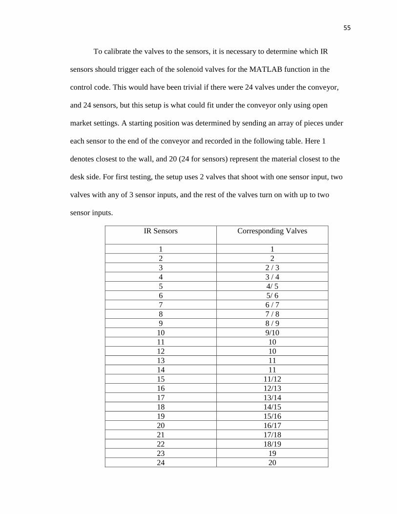
55
To calibrate the valves to the sensors, it is necessary to determine which IR
sensors should trigger each of the solenoid valves for the MATLAB function in the
control code. This would have been trivial if there were 24 valves under the conveyor,
and 24 sensors, but this setup is what could fit under the conveyor only using open
market settings. A starting position was determined by sending an array of pieces under
each sensor to the end of the conveyor and recorded in the following table. Here 1
denotes closest to the wall, and 20 (24 for sensors) represent the material closest to the
desk side. For first testing, the setup uses 2 valves that shoot with one sensor input, two
valves with any of 3 sensor inputs, and the rest of the valves turn on with up to two
sensor inputs.
IR Sensors
Corresponding Valves
1 1
2 2
3 2 / 3
4 3 / 4
5 4/ 5
6 5/ 6
7 6 / 7
8 7 / 8
9 8 / 9
10 9/10
11 10
12 10
13 11
14 11
15 11/12
16 12/13
17 13/14
18 14/15
19 15/16
20 16/17
21 17/18
22 18/19
23 19
24 20
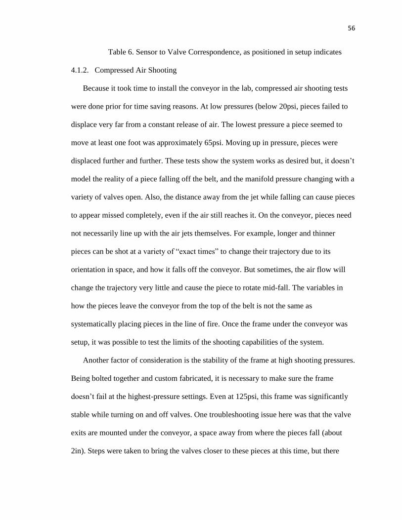
56
Table 6. Sensor to Valve Correspondence, as positioned in setup indicates
4.1.2. Compressed Air Shooting
Because it took time to install the conveyor in the lab, compressed air shooting tests
were done prior for time saving reasons. At low pressures (below 20psi, pieces failed to
displace very far from a constant release of air. The lowest pressure a piece seemed to
move at least one foot was approximately 65psi. Moving up in pressure, pieces were
displaced further and further. These tests show the system works as desired but, it doesn’t
model the reality of a piece falling off the belt, and the manifold pressure changing with a
variety of valves open. Also, the distance away from the jet while falling can cause pieces
to appear missed completely, even if the air still reaches it. On the conveyor, pieces need
not necessarily line up with the air jets themselves. For example, longer and thinner
pieces can be shot at a variety of “exact times” to change their trajectory due to its
orientation in space, and how it falls off the conveyor. But sometimes, the air flow will
change the trajectory very little and cause the piece to rotate mid-fall. The variables in
how the pieces leave the conveyor from the top of the belt is not the same as
systematically placing pieces in the line of fire. Once the frame under the conveyor was
setup, it was possible to test the limits of the shooting capabilities of the system.
Another factor of consideration is the stability of the frame at high shooting pressures.
Being bolted together and custom fabricated, it is necessary to make sure the frame
doesn’t fail at the highest-pressure settings. Even at 125psi, this frame was significantly
stable while turning on and off valves. One troubleshooting issue here was that the valve
exits are mounted under the conveyor, a space away from where the pieces fall (about
2in). Steps were taken to bring the valves closer to these pieces at this time, but there
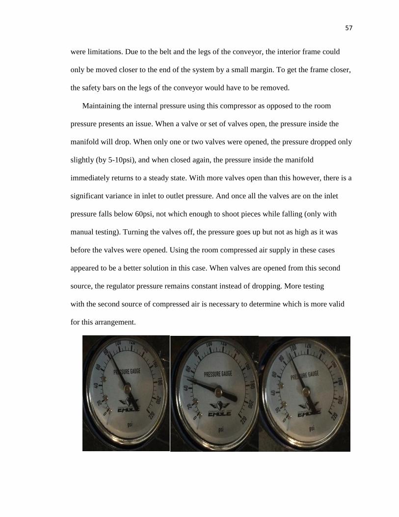
57
were limitations. Due to the belt and the legs of the conveyor, the interior frame could
only be moved closer to the end of the system by a small margin. To get the frame closer,
the safety bars on the legs of the conveyor would have to be removed.
Maintaining the internal pressure using this compressor as opposed to the room
pressure presents an issue. When a valve or set of valves open, the pressure inside the
manifold will drop. When only one or two valves were opened, the pressure dropped only
slightly (by 5-10psi), and when closed again, the pressure inside the manifold
immediately returns to a steady state. With more valves open than this however, there is a
significant variance in inlet to outlet pressure. And once all the valves are on the inlet
pressure falls below 60psi, not which enough to shoot pieces while falling (only with
manual testing). Turning the valves off, the pressure goes up but not as high as it was
before the valves were opened. Using the room compressed air supply in these cases
appeared to be a better solution in this case. When valves are opened from this second
source, the regulator pressure remains constant instead of dropping. More testing
with the second source of compressed air is necessary to determine which is more valid
for this arrangement.
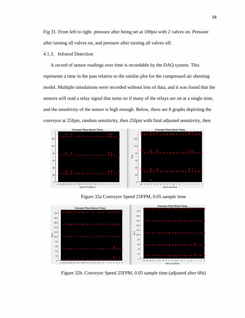
58
Fig 31. From left to right. pressure after being set at 100psi with 2 valves on. Pressure
after turning all valves on, and pressure after turning all valves off.
4.1.3. Infrared Detection
A record of sensor readings over time is recordable by the DAQ system. This
represents a time in the past relative to the similar plot for the compressed air shooting
model. Multiple simulations were recorded without loss of data, and it was found that the
sensors will read a relay signal that turns on if many of the relays are on at a single time,
and the sensitivity of the sensor is high enough. Below, there are 8 graphs depicting the
conveyor at 25fpm, random sensitivity, then 25fpm with final adjusted sensitivity, then
Figure 32a Conveyor Speed 25FPM, 0.05 sample time
Figure 32b. Conveyor Speed 25FPM, 0.05 sample time (adjusted after 60s)
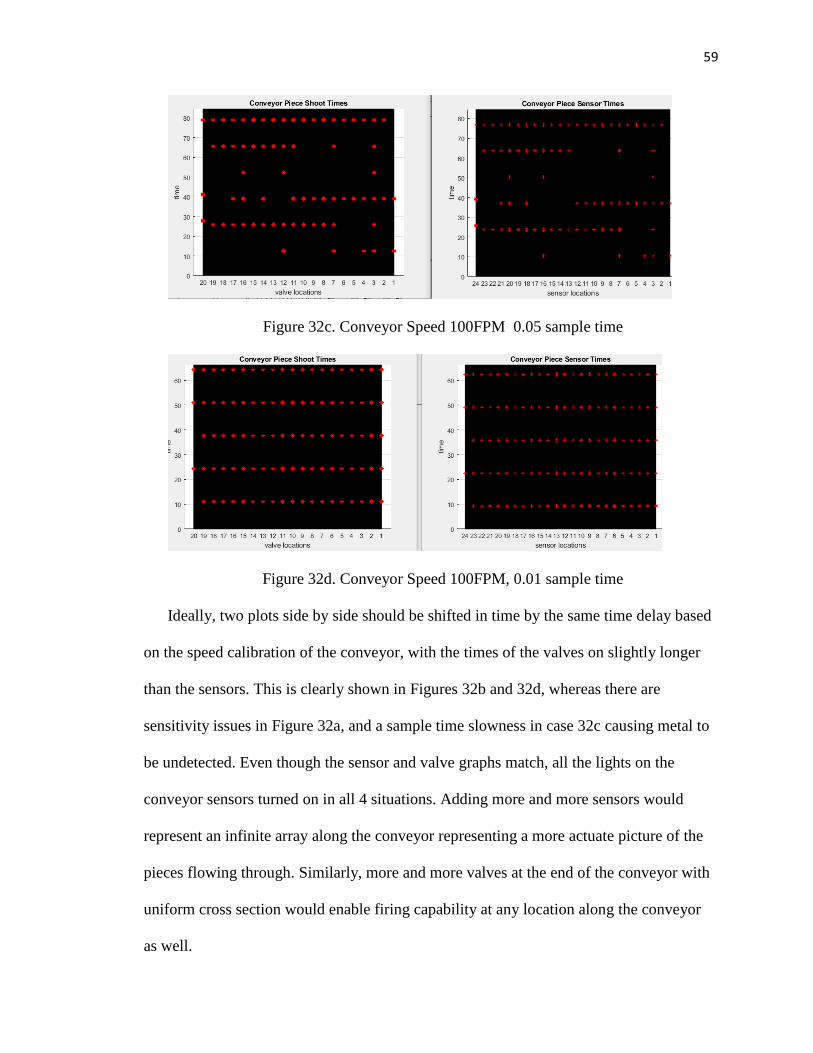
59
Figure 32c. Conveyor Speed 100FPM 0.05 sample time
Figure 32d. Conveyor Speed 100FPM, 0.01 sample time
Ideally, two plots side by side should be shifted in time by the same time delay based
on the speed calibration of the conveyor, with the times of the valves on slightly longer
than the sensors. This is clearly shown in Figures 32b and 32d, whereas there are
sensitivity issues in Figure 32a, and a sample time slowness in case 32c causing metal to
be undetected. Even though the sensor and valve graphs match, all the lights on the
conveyor sensors turned on in all 4 situations. Adding more and more sensors would
represent an infinite array along the conveyor representing a more actuate picture of the
pieces flowing through. Similarly, more and more valves at the end of the conveyor with
uniform cross section would enable firing capability at any location along the conveyor
as well.

60
To calibrate the sensors, they were mounted to the conveyor as shown in Figure 31
and set to a sensitivity at which they wound not receive a reading of the belt underneath.
Then the sensitivities were adjusted such that they would detect a thin piece of metal
directly underneath. This was done through the setting arrangements as well as moving
the sensor diodes (LEDs) into positions. While larger pieces were easily detected, smaller
pieces were not always detectable with space between sensors (about 0.25in between
each sensor with width 0.5in.)
The sensitivity of each sensor plays an important role in the detection of materials. To
calibrate the sensors to the best of our capabilities, some sample pieces were placed under
the sensors and slid from under one sensor to another in a timely fashion. The goal of this
method was to make sure smaller pieces such as the shavings could be detected even
though they are not necessarily aligned with the sensors themselves. The issue with this
method is that the sensors themselves had to be far enough away for larger pieces of
approximately 1 inch to flow through, which means the sensors had to be extremely
sensitive to their surroundings to pick up anything smaller.
Fig 33. IR Sensor Calibration of Aluminum. On and off using conveyor motion.
The sensitivity of the sensor is its ability to change from on to off in the presence of a
material is quite low. While the range of the detectable material was given from 2-30cm,
the sensors only measure up to 2cm. Changing this ever so slightly can cause the sensor
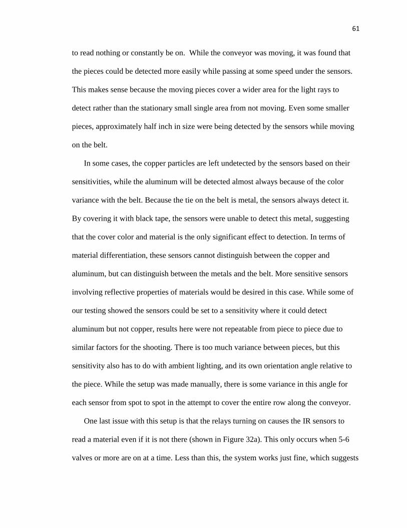
61
to read nothing or constantly be on. While the conveyor was moving, it was found that
the pieces could be detected more easily while passing at some speed under the sensors.
This makes sense because the moving pieces cover a wider area for the light rays to
detect rather than the stationary small single area from not moving. Even some smaller
pieces, approximately half inch in size were being detected by the sensors while moving
on the belt.
In some cases, the copper particles are left undetected by the sensors based on their
sensitivities, while the aluminum will be detected almost always because of the color
variance with the belt. Because the tie on the belt is metal, the sensors always detect it.
By covering it with black tape, the sensors were unable to detect this metal, suggesting
that the cover color and material is the only significant effect to detection. In terms of
material differentiation, these sensors cannot distinguish between the copper and
aluminum, but can distinguish between the metals and the belt. More sensitive sensors
involving reflective properties of materials would be desired in this case. While some of
our testing showed the sensors could be set to a sensitivity where it could detect
aluminum but not copper, results here were not repeatable from piece to piece due to
similar factors for the shooting. There is too much variance between pieces, but this
sensitivity also has to do with ambient lighting, and its own orientation angle relative to
the piece. While the setup was made manually, there is some variance in this angle for
each sensor from spot to spot in the attempt to cover the entire row along the conveyor.
One last issue with this setup is that the relays turning on causes the IR sensors to
read a material even if it is not there (shown in Figure 32a). This only occurs when 5-6
valves or more are on at a time. Less than this, the system works just fine, which suggests

62
that there is a bug when multiple pieces are shot at one time, possibly due to excess
wiring in the DAQ card, which is the only place the two are joined. This can cause issues
when dealing with shooting pieces, because it will lead to more misfires than previously
expected. To get around this issue, the sensors on the conveyor must be adjustable.
4.2.Modifications for Integrated Testing
4.2.1. System Limitations
The SLRT software has some limitations in its programming that must be considered
while using data. The data log buffer in the parameter’s menu can be set for memory
distribution for data logging. While the system runs in real time as planned, the
recordings can be overwritten if the sample time is too small. For our simulations a
sampling rate of 100Hz, and run time of 60 seconds records all data, and provides enough
time for conveyor to feed pieces through. To modify this, file scope blocks were used so
that the system could record more data by saving it to a file on the target PC, instead of
directly exporting it to the host PC. This enables for longer simulation recordings, and
faster sampling times as well. As far as how fast can the system go, the conveyor at 60Hz
(100fpm setting) can be processed in the real time model built on the target. It takes
approximately 1 minute for the code to build successfully, but once it does, it can start
and stop indefinitely provided the proper frequency is set for the shooting times so many
simulations can be run.
For the compressed air, the compressor needs to be on and air needs to fill the system
before the valve power are triggered. However, the valves begin in an on state because
the relays begin in a switched-on state. To modify this, a switch was added to the
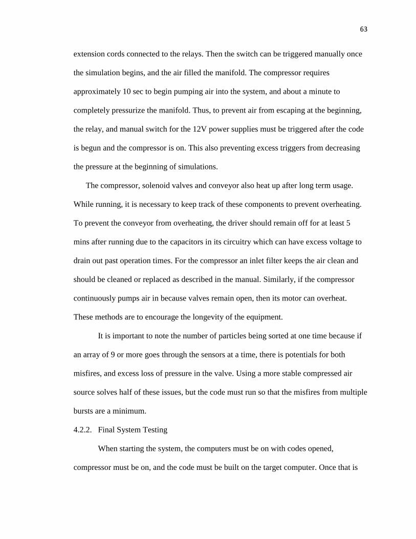
63
extension cords connected to the relays. Then the switch can be triggered manually once
the simulation begins, and the air filled the manifold. The compressor requires
approximately 10 sec to begin pumping air into the system, and about a minute to
completely pressurize the manifold. Thus, to prevent air from escaping at the beginning,
the relay, and manual switch for the 12V power supplies must be triggered after the code
is begun and the compressor is on. This also preventing excess triggers from decreasing
the pressure at the beginning of simulations.
The compressor, solenoid valves and conveyor also heat up after long term usage.
While running, it is necessary to keep track of these components to prevent overheating.
To prevent the conveyor from overheating, the driver should remain off for at least 5
mins after running due to the capacitors in its circuitry which can have excess voltage to
drain out past operation times. For the compressor an inlet filter keeps the air clean and
should be cleaned or replaced as described in the manual. Similarly, if the compressor
continuously pumps air in because valves remain open, then its motor can overheat.
These methods are to encourage the longevity of the equipment.
It is important to note the number of particles being sorted at one time because if
an array of 9 or more goes through the sensors at a time, there is potentials for both
misfires, and excess loss of pressure in the valve. Using a more stable compressed air
source solves half of these issues, but the code must run so that the misfires from multiple
bursts are a minimum.
4.2.2. Final System Testing
When starting the system, the computers must be on with codes opened,
compressor must be on, and the code must be built on the target computer. Once that is
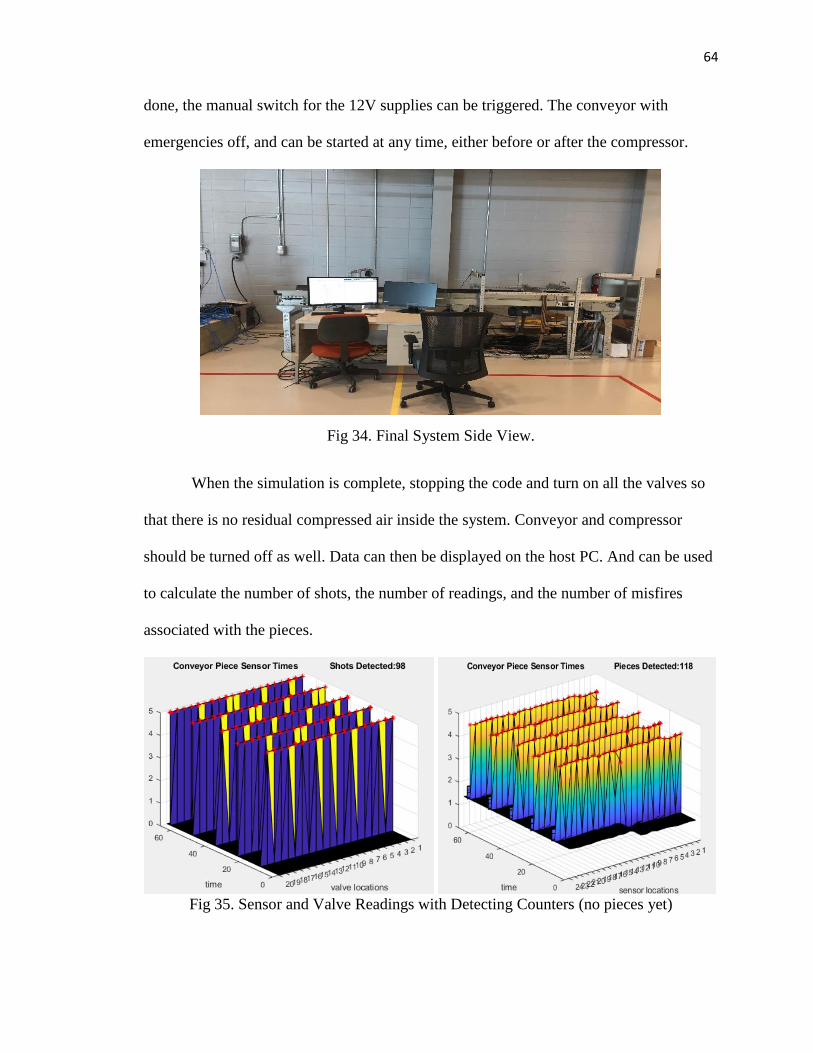
64
done, the manual switch for the 12V supplies can be triggered. The conveyor with
emergencies off, and can be started at any time, either before or after the compressor.
Fig 34. Final System Side View.
When the simulation is complete, stopping the code and turn on all the valves so
that there is no residual compressed air inside the system. Conveyor and compressor
should be turned off as well. Data can then be displayed on the host PC. And can be used
to calculate the number of shots, the number of readings, and the number of misfires
associated with the pieces.
Fig 35. Sensor and Valve Readings with Detecting Counters (no pieces yet)
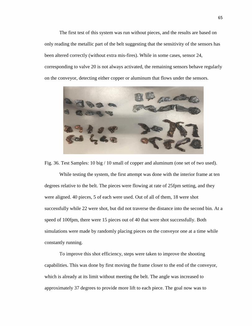
65
The first test of this system was run without pieces, and the results are based on
only reading the metallic part of the belt suggesting that the sensitivity of the sensors has
been altered correctly (without extra mis-fires). While in some cases, sensor 24,
corresponding to valve 20 is not always activated, the remaining sensors behave regularly
on the conveyor, detecting either copper or aluminum that flows under the sensors.
Fig. 36. Test Samples: 10 big / 10 small of copper and aluminum (one set of two used).
While testing the system, the first attempt was done with the interior frame at ten
degrees relative to the belt. The pieces were flowing at rate of 25fpm setting, and they
were aligned. 40 pieces, 5 of each were used. Out of all of them, 18 were shot
successfully while 22 were shot, but did not traverse the distance into the second bin. At a
speed of 100fpm, there were 15 pieces out of 40 that were shot successfully. Both
simulations were made by randomly placing pieces on the conveyor one at a time while
constantly running.
To improve this shot efficiency, steps were taken to improve the shooting
capabilities. This was done by first moving the frame closer to the end of the conveyor,
which is already at its limit without meeting the belt. The angle was increased to
approximately 37 degrees to provide more lift to each piece. The goal now was to
66
determine how many pieces could be shot, how many would be missed, and how many
extra fires the system will cause. This data can easily be obtained from the variables
recorded from the Simulink blocks. While precise shooting remains an issue for this
design, there are some benefits to this layout, providing an easy way to adjust the setup to
achieve more promising results of the sorting applications in the future.
4.3. Future Improvements and Applications
Future testing needs to be done to determine the precise parameters that will suffice
for this setup. With all the geometry, and calculations, there is still some uncertainties
starting with time delay for every piece. Because the interior frame with solenoids and
the IR sensors is completely separated from the conveyor, there is the potential of being
misaligned, which can affect the sorting time in small but significant ways. Even though
the IR sensors were set up so that they could not detect the belt, they control the state of
the relays. Day to day however, these sensors do not always have the same readings and
must be readjusted. Something more controllable, predictable and reliable such as
computer vision might be tried.
The pressure inside the manifold is not constant. Even though the pressures go up
to 125psi at turn on, the pressure in the system decreases over time. Due to the plumber’s
tape on the manifold and valves, there are not any significant leaks. Another problem
with the compressed air is that the valves are spaced one inch apart, leaving space for
pieces to fall between the valves, making them difficult (not impossible) to shoot. The
orientation of some of these pieces is significant to whether they are hit. This is another
place where computer vision would come in handy. Another addition that might be useful

67
for this system is the ability to read the pressure in the manifold in real time to determine
at what times the pressure goes down significantly and hinders the system. This could be
accomplished in many ways. One is by using electrical pressure gauges, or pitot tubes at
the exit valves.
The primary shortcoming of this system is that now it cannot differentiate by
material. In some cases, we were able to adjust the sensitivity of some IR sensors so that
the aluminum would reflect more, and the copper would not. However, this method was
not repeatable. The sensitivity, and uncertainties with the IR sensors were just too great.
To improve the system, the most significant improvement would be to use
computer vision, or some other sensor that would enable the determination of each piece
in real time on the conveyor. Next steps would be to configure the compressed air to
shoot pieces much further, maintain even higher pressures longer, without having relays
trigger IR signals independently. The reason the IR sensors were placed above is because
it was not sure as to how fast the Simulink real-time system would behave. Now that the
real time applications have been tested, this system could seem to benefit from an “in air
sort” versus having time delays in the program at all [19]. In summary, the main
improvements needed for this system are more hardware related then in design concept.
68
5. Conclusions
This system was designed to shoot and sort pieces of copper and aluminum
autonomously, but there is still work to be done. The conveyor, compressor, frames, and
safety precautions were fabricated, troubleshooted, and implemented into the final system
with very little variance to the approved design. The control algorithm implemented
proved to be useful in timing the shots of the metal pieces.
The setup is enough for testing means and models real world industrial recycling
models such as MSS correctly. Like those systems, the parameters are adjustable,
regarding method of detection, compressed air shooting, angle of shooting, and code
parameters such as time delays, and shooting times. Simulink real-time proved to be
useful in performing the real time application of this conveyor, as well recording the data
from the NI 6259 DAQ card.
The conveyor acts as intended with variable speed, and safety features, housing
the wiring and computers underneath. The framing proved to be very flexible, allowing
for multiple options in the hardware side of future projects. The sorting chamber acts as a
very good barrier, preventing anyone in the lab from being injured by compressed air
valves and the pieces of metal they shoot. While, the manifold tends to decrease in
pressure from its max over time, the valves and the IR sensors can be directly connected
by one function, enabling a wide variety of applications as options. Even though it has
been shown that pieces can be shot, more efficient methods of shooting must be
implemented to improve the system. Furthermore, this system can benefit significantly
from computer vision applications. The goal of this project was to design, fabricate, and
test a conveyor sorting system. While more tests still need to be done, the overall system
69
needs very few adjustments. Perhaps a more effective row of valves is possible for a
position under the conveyor or looking down on it from above with a more precise sort is
possible. All things considered, this system is performing as intended and it is still
moving forward. Recent developments in the recycling industry such as China refusing
imports with less than 99.5% purity, plastic production estimated to grow exponentially,
the profitability involved with recycling both economic, and environmental cannot be
ignored [32]. Developing this system provides a means to demonstrate the fundamental
principles in a recycling system and recover data to analyze methods in recycling for the
future.

70
Appendix A. MATLAB Codes
Code 1: Operation Start Up
%Computer Parameters
T_run = inf;
T_sample = 0.05;
t_shoot= T_sample*10; %time to leave valve on
frequency = 15; %Hz - Conveyor Start Speed
%Calibrations: %Relays Works 5V = OFF, 0V = ON %IR Sensors
work like 3-4V triggered off, 0.3-0.4V triggered by piece.
%Sensor to Valve Time Calibration
fsample = 1/T_sample; speed = 5/3*frequency; %fpm
deltax = 33.5/12;
t_delay = deltax/speed*60; %time to wait from sensor.
%Record Times from Turn on location to exit.
f=15:5:60;
times_theoretical = deltax./(5/3*f)*60;
times_measured = …
[6.0,4.39,3.69,3.09,2.65,2.32,2.12,1.80,1.73,1.67];
time_error = (times_theoretical-times_measured);
v_theoretical = f.*5/3;
v_measured = deltax./(times_measured/60);
v_error = abs((v_theoretical -
v_measured))./v_theoretical*100;
%Calibration Curves (linear fit for speed)
P=polyfit(f,v_measured,1);
speed_calibration =@(z) P(1).*z+P(2);
time_calibration =@(z) deltax./(P(1)*z+P(2))*60;
r_v=1-sum((speed_calibration(f)-
v_measured).^2)/sum(v_measured.^2); r_t=1-
sum((time_calibration(f)-
times_measured).^2)/sum(times_measured.^2);
figure(1)
plot(f,v_theoretical,'r-o',f,v_measured,'bo-…
',f,v_error,'go-')
hold on
fplot(speed_calibration,[15,60],'y-o')
xlabel('frequency (Hz)') ylabel('Conveyor Speed (fpm)')
legend('theoretical speed','belt speed','error …
%',['regression=',num2str(P(1)),'f+',num2str(P(2))],'locati
on','nw')
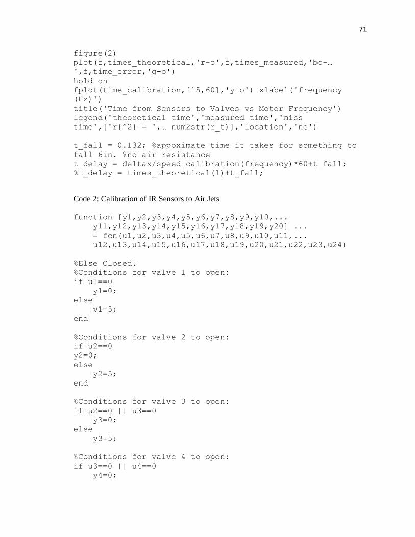
71
figure(2)
plot(f,times_theoretical,'r-o',f,times_measured,'bo-…
',f,time_error,'g-o')
hold on
fplot(time_calibration,[15,60],'y-o') xlabel('frequency
(Hz)')
title('Time from Sensors to Valves vs Motor Frequency')
legend('theoretical time','measured time','miss
time',['r{^2} = ',… num2str(r_t)],'location','ne')
t_fall = 0.132; %appoximate time it takes for something to
fall 6in. %no air resistance
t_delay = deltax/speed_calibration(frequency)*60+t_fall;
%t_delay = times_theoretical(1)+t_fall;
Code 2: Calibration of IR Sensors to Air Jets
function [y1,y2,y3,y4,y5,y6,y7,y8,y9,y10,...
y11,y12,y13,y14,y15,y16,y17,y18,y19,y20] ...
= fcn(u1,u2,u3,u4,u5,u6,u7,u8,u9,u10,u11,...
u12,u13,u14,u15,u16,u17,u18,u19,u20,u21,u22,u23,u24)
%Else Closed.
%Conditions for valve 1 to open:
if u1==0
y1=0;
else
y1=5;
end
%Conditions for valve 2 to open:
if u2==0
y2=0;
else
y2=5;
end
%Conditions for valve 3 to open:
if u2==0 || u3==0
y3=0;
else
y3=5;
%Conditions for valve 4 to open:
if u3==0 || u4==0
y4=0;
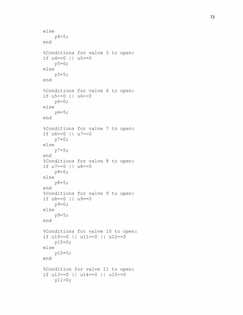
72
else
y4=5;
end
%Conditions for valve 5 to open:
if u4==0 || u5==0
y5=0;
else
y5=5;
end
%Conditions for valve 6 to open:
if u5==0 || u6==0
y6=0;
else
y6=5;
end
%Conditions for valve 7 to open:
if u6==0 || u7==0
y7=0;
else
y7=5;
end
%Conditions for valve 8 to open:
if u7==0 || u8==0
y8=0;
else
y8=5;
end
%Conditions for valve 9 to open:
if u8==0 || u9==0
y9=0;
else
y9=5;
end
%Conditions for valve 10 to open:
if u10==0 || u11==0 || u12==0
y10=0;
else
y10=5;
end
%Condition for valve 11 to open:
if u13==0 || u14==0 || u15==0
y11=0;
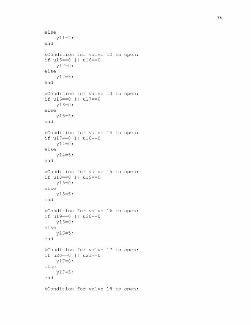
73
else
y11=5;
end
%Condition for valve 12 to open:
if u15==0 || u16==0
y12=0;
else
y12=5;
end
%Condition for valve 13 to open:
if u16==0 || u17==0
y13=0;
else
y13=5;
end
%Condition for valve 14 to open:
if u17==0 || u18==0
y14=0;
else
y14=5;
end
%Condition for valve 15 to open:
if u18==0 || u19==0
y15=0;
else
y15=5;
end
%Condition for valve 16 to open:
if u19==0 || u20==0
y16=0;
else
y16=5;
end
%Condition for valve 17 to open:
if u20==0 || u21==0
y17=0;
else
y17=5;
end
%Condition for valve 18 to open:
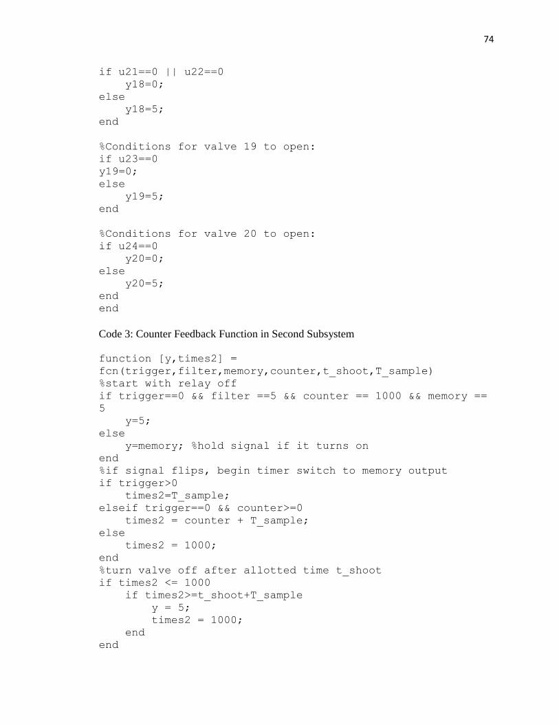
74
if u21==0 || u22==0
y18=0;
else
y18=5;
end
%Conditions for valve 19 to open:
if u23==0
y19=0;
else
y19=5;
end
%Conditions for valve 20 to open:
if u24==0
y20=0;
else
y20=5;
end
end
Code 3: Counter Feedback Function in Second Subsystem
function [y,times2] =
fcn(trigger,filter,memory,counter,t_shoot,T_sample)
%start with relay off
if trigger==0 && filter ==5 && counter == 1000 && memory ==
5
y=5;
else
y=memory; %hold signal if it turns on
end
%if signal flips, begin timer switch to memory output
if trigger>0
times2=T_sample;
elseif trigger==0 && counter>=0
times2 = counter + T_sample;
else
times2 = 1000;
end
%turn valve off after allotted time t_shoot
if times2 <= 1000
if times2>=t_shoot+T_sample
y = 5;
times2 = 1000;
end
end
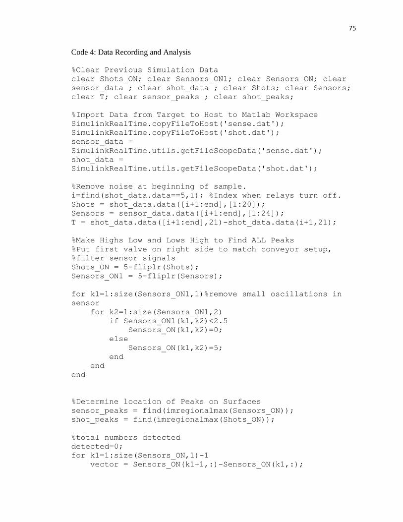
75
Code 4: Data Recording and Analysis
%Clear Previous Simulation Data
clear Shots_ON; clear Sensors_ON1; clear Sensors_ON; clear
sensor_data ; clear shot_data ; clear Shots; clear Sensors;
clear T; clear sensor_peaks ; clear shot_peaks;
%Import Data from Target to Host to Matlab Workspace
SimulinkRealTime.copyFileToHost('sense.dat');
SimulinkRealTime.copyFileToHost('shot.dat');
sensor_data =
SimulinkRealTime.utils.getFileScopeData('sense.dat');
shot_data =
SimulinkRealTime.utils.getFileScopeData('shot.dat');
%Remove noise at beginning of sample.
i=find(shot_data.data==5,1); %Index when relays turn off.
Shots = shot_data.data([i+1:end],[1:20]);
Sensors = sensor_data.data([i+1:end],[1:24]);
T = shot_data.data([i+1:end],21)-shot_data.data(i+1,21);
%Make Highs Low and Lows High to Find ALL Peaks
%Put first valve on right side to match conveyor setup,
%filter sensor signals
Shots_ON = 5-fliplr(Shots);
Sensors_ON1 = 5-fliplr(Sensors);
for k1=1:size(Sensors_ON1,1)%remove small oscillations in
sensor
for k2=1:size(Sensors_ON1,2)
if Sensors_ON1(k1,k2)<2.5
Sensors_ON(k1,k2)=0;
else
Sensors_ON(k1,k2)=5;
end
end
end
%Determine location of Peaks on Surfaces
sensor_peaks = find(imregionalmax(Sensors_ON));
shot_peaks = find(imregionalmax(Shots_ON));
%total numbers detected
detected=0;
for k1=1:size(Sensors_ON,1)-1
vector = Sensors_ON(k1+1,:)-Sensors_ON(k1,:);
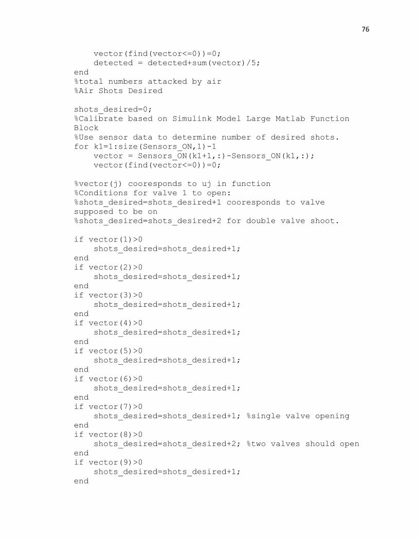
76
vector(find(vector<=0))=0;
detected = detected+sum(vector)/5;
end
%total numbers attacked by air
%Air Shots Desired
shots_desired=0;
%Calibrate based on Simulink Model Large Matlab Function
Block
%Use sensor data to determine number of desired shots.
for k1=1:size(Sensors_ON,1)-1
vector = Sensors_ON(k1+1,:)-Sensors_ON(k1,:);
vector(find(vector<=0))=0;
%vector(j) cooresponds to uj in function
%Conditions for valve 1 to open:
%shots_desired=shots_desired+1 cooresponds to valve
supposed to be on
%shots_desired=shots_desired+2 for double valve shoot.
if vector(1)>0
shots_desired=shots_desired+1;
end
if vector(2)>0
shots_desired=shots_desired+1;
end
if vector(3)>0
shots_desired=shots_desired+1;
end
if vector(4)>0
shots_desired=shots_desired+1;
end
if vector(5)>0
shots_desired=shots_desired+1;
end
if vector(6)>0
shots_desired=shots_desired+1;
end
if vector(7)>0
shots_desired=shots_desired+1; %single valve opening
end
if vector(8)>0
shots_desired=shots_desired+2; %two valves should open
end
if vector(9)>0
shots_desired=shots_desired+1;
end
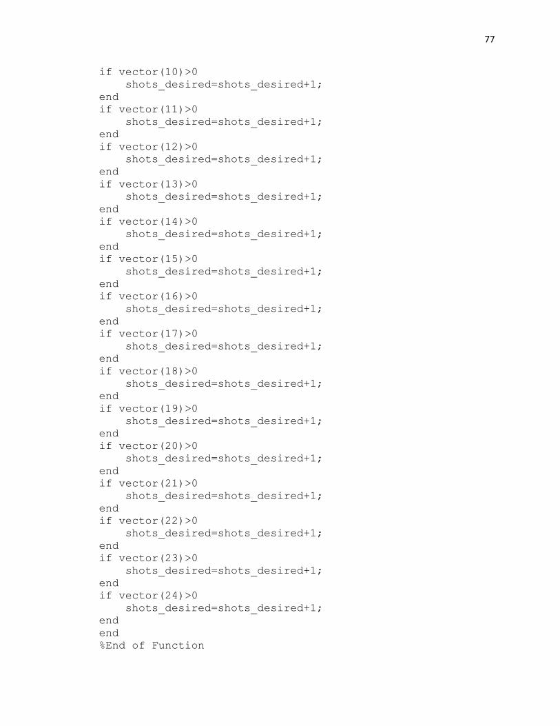
77
if vector(10)>0
shots_desired=shots_desired+1;
end
if vector(11)>0
shots_desired=shots_desired+1;
end
if vector(12)>0
shots_desired=shots_desired+1;
end
if vector(13)>0
shots_desired=shots_desired+1;
end
if vector(14)>0
shots_desired=shots_desired+1;
end
if vector(15)>0
shots_desired=shots_desired+1;
end
if vector(16)>0
shots_desired=shots_desired+1;
end
if vector(17)>0
shots_desired=shots_desired+1;
end
if vector(18)>0
shots_desired=shots_desired+1;
end
if vector(19)>0
shots_desired=shots_desired+1;
end
if vector(20)>0
shots_desired=shots_desired+1;
end
if vector(21)>0
shots_desired=shots_desired+1;
end
if vector(22)>0
shots_desired=shots_desired+1;
end
if vector(23)>0
shots_desired=shots_desired+1;
end
if vector(24)>0
shots_desired=shots_desired+1;
end
end
%End of Function
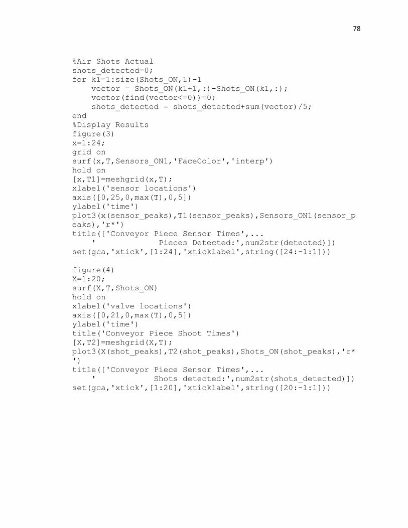
78
%Air Shots Actual
shots_detected=0;
for k1=1:size(Shots_ON,1)-1
vector = Shots_ON(k1+1,:)-Shots_ON(k1,:);
vector(find(vector<=0))=0;
shots_detected = shots_detected+sum(vector)/5;
end
%Display Results
figure(3)
x=1:24;
grid on
surf(x,T,Sensors_ON1,'FaceColor','interp')
hold on
[x,T1]=meshgrid(x,T);
xlabel('sensor locations')
axis([0,25,0,max(T),0,5])
ylabel('time')
plot3(x(sensor_peaks),T1(sensor_peaks),Sensors_ON1(sensor_p
eaks),'r*')
title(['Conveyor Piece Sensor Times',...
' Pieces Detected:',num2str(detected)])
set(gca,'xtick',[1:24],'xticklabel',string([24:-1:1]))
figure(4)
X=1:20;
surf(X,T,Shots_ON)
hold on
xlabel('valve locations')
axis([0,21,0,max(T),0,5])
ylabel('time')
title('Conveyor Piece Shoot Times')
[X,T2]=meshgrid(X,T);
plot3(X(shot_peaks),T2(shot_peaks),Shots_ON(shot_peaks),'r*
')
title(['Conveyor Piece Sensor Times',...
' Shots detected:',num2str(shots_detected)])
set(gca,'xtick',[1:20],'xticklabel',string([20:-1:1]))
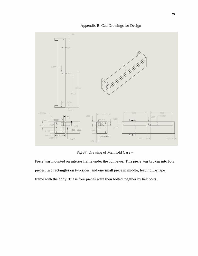
79
Appendix B. Cad Drawings for Design
Fig 37. Drawing of Manifold Case –
Piece was mounted on interior frame under the conveyor. This piece was broken into four
pieces, two rectangles on two sides, and one small piece in middle, leaving L-shape
frame with the body. These four pieces were then bolted together by hex bolts.
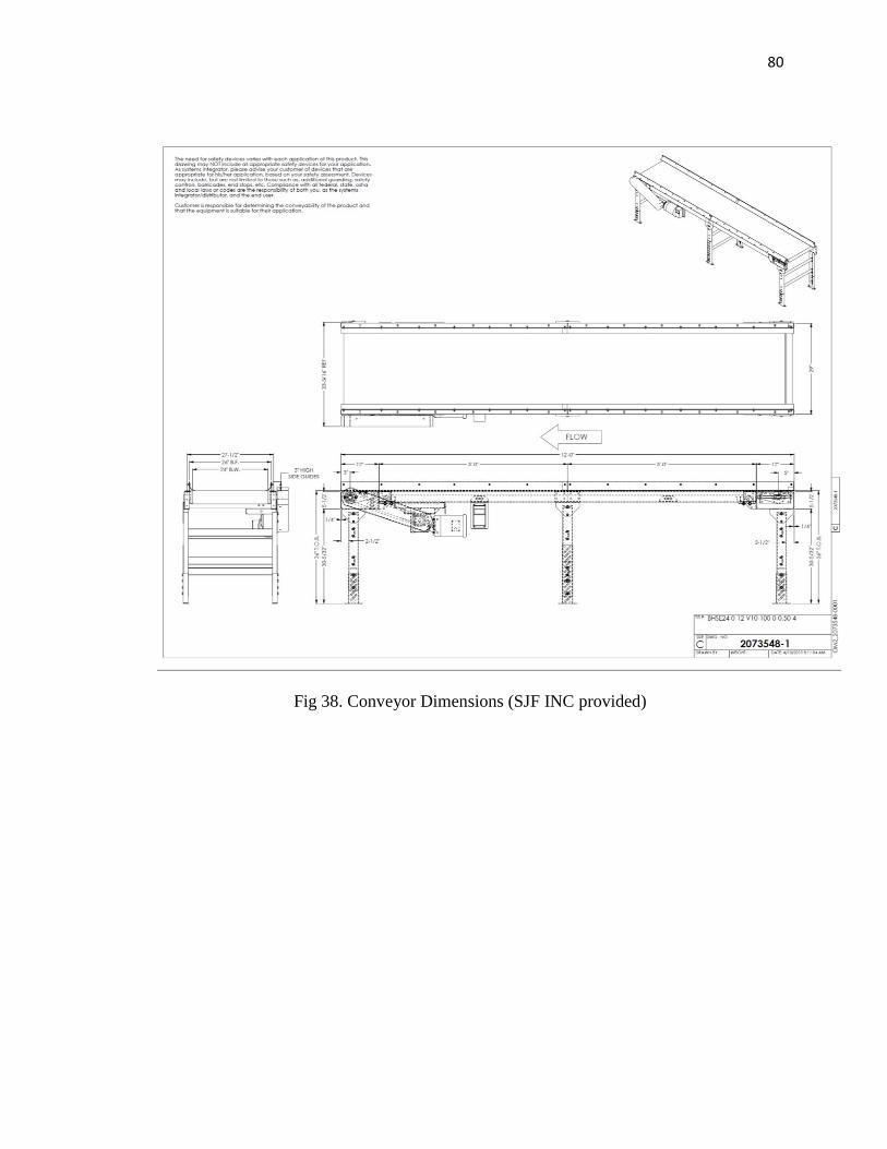
80
Fig 38. Conveyor Dimensions (SJF INC provided)

81
References
[1] “Zero Waste Versus Recycling: What’s the Difference?” Sustainable Jungle Inc.
2019. Accessed: 6 July 2019. Web. https://www.sustainablejungle.com/sustainable-
living/zero-waste-future/
[2] “7 Things you didn’t know about Plastics and Recycling.” National Geographic. April
4 2018. Accessed 6 July 2019. Web. https://blog.nationalgeographic.org/2018/04/04/7-
things-you-didnt-know-about-plastic-and-recycling/
[3] “Sorting.” Wikipedia, the Free Encyclopedia. Accessed: 1 March 2019. Web.
https://en.wikipedia.org/wiki/Sorting
[4] “About Sensor Based Sorting” Tomra. Accessed: 6 July 2019. Web.
https://www.tomra.com/en/sorting/mining/about-sensor-based-sorting
[5] “Grading and Sorting” RSIP VISION. Accessed: 6 July 2019. Web.
https://www.rsipvision.com/grading-and-sorting/
[6] Holmes, Audrey. “How many times can that be recycled?.” Earth 911. June 15 2017.
Accessed: 1 March 2019. Web. https://earth911.com/business-policy/how-many-times-
recycled/
[7] “Understanding Single vs Dual Stream Recycling.” Vangel. Accessed 1 July 2019.
Web. https://vangelinc.com/single-vs-dual-stream-recycling/
[8] “How a Materials Recovery Facility Works.” Dacota Valley Recycling. Accessed: 1
March 2019. Web. https://www.dakotavalleyrecycling.org/component/tags/tag/garbage
[9] Haitb, Subrata, Gundupalli, Sathish Paulraj, Thakurc, Atul. “A Review on Automated
Sorting of Source-separated Municipal Solid Waste for Recycling.” Waste Management
February 2017. PDF.
[10] Conclaves, Andressa Dancini. “Metallic Reflection” eng.libretexts.org. MindTouch.
Figure 4. Web. 18 April 2018. Accessed: Nov 25 2018.
https://eng.libretexts.org/Textbook_Maps/Chemical_Engineering/Supplemental_Modules
_(Materials_Science)/Optical_Properties/Metallic_Reflection
[11] LeBlanc, Rick. “Auto Recycling Recent Trends, Opportunities, and Challenges.”
Sustainable Businesses. Thebalancesmb.com. Updated: Feb. 26, 2019. Accessed: 19
March 2019. https://www.thebalancesmb.com/auto-recycling-recent-trends-
opportunities-and-challenges-4011892
[12] LeBlanc, Rick. “Airplane Recycling and Value Extraction.” Sustainable Businesses.
Thebalancesmb.com. Updated: Nov. 18, 2018. Accessed: 19 March 2019.
https://www.thebalancesmb.com/airplane-recycling-and-value-extraction-2877922

82
[13] Baranuik, Chris. How algorithms run Amazon Warehouses. Future. BBC.com.
2019. August 18 2015. Accessed: 19 March 2019. Web.
http://www.bbc.com/future/story/20150818-how-algorithms-run-amazons-warehouses
[14] Sortation Conveyors. REB Storage Systems International. Accessed 6 July 2019.
Web. https://rebstorage.com/our-products/conveyors/sortation-conveyors/
[15] Adeoye, A.O.M., Aghor, A. Esoso, Balogun, V.A., Daniyan I.A., Ijagbemi, C.O.
Oladapo, Bankole I., Oluwole, Afolabi S. Simeon, Asanta P. “Model Design and
Simulation of Automatic Sorting Machine using proximity sensor.” Engineering Science
and Technology, An International Journal. Revised: 25 April 2016. PDF.
[16] Ritchie, Hannah. “FAQS on Plastics”. Our World in Data. 2018 September 2.
Accessed 19 March 2019. Web. https://ourworldindata.org/faq-on-plastics
[17] “Challenges of pastic waste disposal in Ghana: a case study of solid ways disposal
sites in Accra.” Management Arts. Elixir International Journal. Web. Accessed: 19 March
2019. https://www.elixirpublishers.com/articles/1350467591_49%20(2012)%209879-
9885.pdf
[18] Recycling Technology. Tomra-Recycling Technology. 12 December 2018 Web.
https://www.tomra.com/en/sorting/recycling/recycling-technology
[19] “MSS Optical Sorting Technology.” cpgrp.com. mssoptical.com. pg 1-8. Powered by
Flippingbook. ‘Catalog’. Web. Accessed: October 14 2018.
http://www.cpgrp.com/mss-brochure/files/assets/basic-html/page-8.html
[20] “How to keep a belt on track.” Flexco. 2018 August. Accessed: 19 March 2019.
Web. https://www.flexco.com/EN/Blogs/How-To-Keep-Your-Conveyor-Belt-on-
Track.htm
[21] Connectors. McMasterCarr. Accessed. 14 October 2018. Web.
https://www.mcmaster.com/8809t52
[22] Rogers, Tony. “Everything you need to know about Polycarbonate.” Creative
Mechanisms Blog. 2015 August 21. Accessed 10 November 2019. Web.
https://www.creativemechanisms.com/blog/everything-you-need-to-know-about-
polycarbonate-pc
[23] Pneumandyne Catalog 2400. Pneumadyne.com. Accessed 10 Nov 2018. Web.
https://www.pneumadyne.com/documents/PDFs/Full%20Line%20Catalog%202300.pdf
[24] Eagle Silent Series 1.5HP 5.5 Gallons. Air Cpmpressors Direct.com. Power
Equipment Direct. Accessed 2 December 2018. Web.
https://www.aircompressorsdirect.com/Eagle-EA-5000-Air-Compressor/p70903.html

83
[25] “How to Choose the Right Bus for your measurement System.” National
Instruments. Updated May 24 2019. Accessed 6 June 2019. Web.
http://www.ni.com/en-us/innovations/white-papers/09/how-to-choose-the-right-bus-for-
your-measurement-system.html
[26] “Supported Hardware: Hardware Drivers.” Simulink Real Time. Mathworks. 2019.
Web. https://www.mathworks.com/programs/products/simulink-real-
time/supported/hardware-drivers.html
[27] “NI 6259 Device Specifications.” National Instruments. Accessed 1 March 2019.
Web. http://www.ni.com/pdf/manuals/375216c.pdf
[28] “PCI Bus Ethernet Setup.” Simulink Real Time. Mathworks. Documentation
R2017b. Web. https://www.mathworks.com/help/releases/R2017b/xpc/gs/pci-bus-
ethernet-card-setup.html
[29] “Patch Cable vs Crossover Cable: What’s the Difference.” FS. 2016 February 2017.
Accessed: 10 February 2019. https://community.fs.com/blog/patch-cable-vs-crossover-
cable.html
[30] Simulink Real Time Version 6.0. XPC Target Supported Ethernet Chipsets. 2014.
Mathworks. https://www.bitmarker.de/wp-content/uploads/2015/01/xpc-target-supported-
ethernet-chipsets.pdf
[31] “Set up Microsoft Visual Studio 2017 for Simulink Real Time.” MATLAB Answers.
MAthworks. Web. https://www.mathworks.com/matlabcentral/answers/348269-how-do-
i-set-up-microsoft-visual-studio-2017-for-slrt
[32] Bell. Trudy E. “Trashed! Engineering towards Zero Waste”. The Bent of Tau Beta
Pi. Spring 2019. Pg 6-11.
[33] “10 Station Solenoid Manifolds.” Solenoid Valves. Pneumadyne Inc. Web. Accessed
10 December 2018. https://www.pneumadyne.com/station-solenoid-manifolds-p-
1508.html?cPath=77_104_106&ref_id=1513#1-YToxOntzOjQ6ImdyaWQiO2k6MDt9
[34] “Spade Connector.” Solenoid Valves. Pneumadyne Inc. Web. Accessed 10
December 2018. https://www.pneumadyne.com/spade-connector-p-
1311.html?cPath=77_89_90&ref_id=1315#products-performance_data-1311-9610