Embed Size (px)
Citation preview
Michigan Technological University Michigan Technological University
Digital Commons @ Michigan Tech Digital Commons @ Michigan Tech
Dissertations, Master's Theses and Master's Reports - Open
Dissertations, Master's Theses and Master's Reports
2013
SYSTEM DYNAMICS MODELING AS A QUANTITATIVE-SYSTEM DYNAMICS MODELING AS A QUANTITATIVE-
QUALITATIVE FRAMEWORK FOR SUSTAINABLE WATER QUALITATIVE FRAMEWORK FOR SUSTAINABLE WATER
RESOURCES MANAGEMENT: INSIGHTS FOR WATER QUALITY RESOURCES MANAGEMENT: INSIGHTS FOR WATER QUALITY
POLICY IN THE GREAT LAKES REGION POLICY IN THE GREAT LAKES REGION
Ali Mirchi Michigan Technological University
Follow this and additional works at: https://digitalcommons.mtu.edu/etds
Part of the Water Resource Management Commons
Copyright 2013 Ali Mirchi
Recommended Citation Recommended Citation Mirchi, Ali, "SYSTEM DYNAMICS MODELING AS A QUANTITATIVE-QUALITATIVE FRAMEWORK FOR SUSTAINABLE WATER RESOURCES MANAGEMENT: INSIGHTS FOR WATER QUALITY POLICY IN THE GREAT LAKES REGION", Dissertation, Michigan Technological University, 2013. https://doi.org/10.37099/mtu.dc.etds/636
Follow this and additional works at: https://digitalcommons.mtu.edu/etds
Part of the Water Resource Management Commons
SYSTEM DYNAMICS MODELING AS A QUANTITATIVE-
QUALITATIVE FRAMEWORK FOR SUSTAINABLE WATER
RESOURCES MANAGEMENT: INSIGHTS FOR WATER
QUALITY POLICY IN THE GREAT LAKES REGION
By
Ali Mirchi
A DISSERTATION
Submitted in partial fulfillment of the requirements for the degree of
DOCTOR OF PHILOSOPHY
In Civil Engineering
MICHIGAN TECHNOLOGICAL UNIVERSITY
2013
Copyright© 2013 Ali Mirchi 2013

This dissertation has been approved in partial fulfillment of the requirements for the
Degree of DOCTOR OF PHILOSOPHY in Civil Engineering.
Department of Civil and Environmental Engineering
Dissertation Advisor: Dr. David W. Watkins
Committee Member: Dr. Alex S. Mayer
Committee Member: Dr. Daya Muralidharan
Committee Member: Dr. Kaveh Madani
Department Chair: Dr. David Hand
iii
Table of Contents
List of Figures ....................................................................................................................vi
List of Tables....................................................................................................................viii
Preface................................................................................................................................. x
Acknowledgements ........................................................................................................... xii
Abstract ............................................................................................................................. xv
Chapter 1- Background and objectives ........................................................................... 1
1.1. Introduction .......................................................................................................... 1
1.2. Chronological synthesis of watershed modeling .................................................. 3
1.3. Water resources modeling methods and approaches............................................ 8
1.3.1. Modeling methods: Simulation and optimization ......................................... 8
1.3.2. Modeling approaches: Scope and problems addressed ............................... 10
1.4. Objectives and organization ............................................................................... 15
1.5. References .......................................................................................................... 17
Chapter 2- Synthesis of system dynamics tools for holistic conceptualization of water resources problems ........................................................................................................ 22
2.1. Abstract .............................................................................................................. 22
2.2. Introduction ........................................................................................................ 23
2.3. System dynamics and water resources ............................................................... 27
2.4. Qualitative modeling tools in system dynamics ................................................. 32
2.4.1. Causal relationships .................................................................................... 33
2.4.2. Causal loop diagrams and basic feedback loops ......................................... 34
2.4.3. Stock and flow diagrams ............................................................................. 38
2.4.4. Reference modes ......................................................................................... 41
2.4.5. System archetypes ....................................................................................... 43
2.5. Discussion .......................................................................................................... 51
2.5.1. Qualitative versus quantitative modeling.................................................... 51
2.5.2. Validation of system dynamics models ...................................................... 54
2.5.3. Strengths and limitations of system dynamics modeling ............................ 55
iv
2.6. Conclusions ........................................................................................................ 57
2.7. References .......................................................................................................... 59
Chapter 3 - A systems approach to holistic TMDL policy: Case of Lake Allegan, Michigan ........................................................................................................................... 67
3.1. Abstract .............................................................................................................. 67
3.2. Introduction ........................................................................................................ 68
3.3. Lake Allegan’s Eutrophication Problem ............................................................ 71
3.4. System Dynamics and Archetypes ..................................................................... 74
3.5. Model and Data Inputs ....................................................................................... 77
3.6. Model Verification ............................................................................................. 84
3.7. Scenario Simulation Results............................................................................... 87
3.8. Discussion .......................................................................................................... 94
3.9. Conclusions ........................................................................................................ 96
3.10. References ...................................................................................................... 98
Chapter 4 - A high-level simulation-optimization framework for non-point source phosphorus load reduction in the Kalamazoo River watershed (Michigan, USA) ......... 105
4.1. Abstract ............................................................................................................ 105
4.2. Introduction ...................................................................................................... 106
4.3. Data and methods ............................................................................................. 111
4.3.1. Study area.................................................................................................. 111
4.3.2. Simulation-optimization framework ......................................................... 112
4.3.3. System dynamics simulation..................................................................... 115
4.3.4. Optimization model .................................................................................. 117
4.4. Best management practices .............................................................................. 119
4.5. Results and Discussion ..................................................................................... 123
4.5.1. Least-cost BMP set ................................................................................... 123
4.5.2. Effect of socioeconomic growth ............................................................... 125
4.5.3. Uncertainty in TMDL planning ................................................................ 129
4.5.4. The Kalamazoo River watershed’s TMDL ............................................... 133
4.5.5. Limitations ................................................................................................ 136
v
4.6. Conclusions ...................................................................................................... 137
4.7. References ........................................................................................................ 139
Chapter 5 - Market-based policy instruments for mitigating agricultural phosphorus loads in the Maumee Basin ...................................................................................................... 149
5.1. Introduction ...................................................................................................... 149
5.2. Method ............................................................................................................. 152
5.2.1. Problem definition and study area ............................................................ 153
5.2.2. Biophysical model .................................................................................... 156
5.2.3. BMP and agro-economic optimization model .......................................... 158
5.3. Results and discussion ...................................................................................... 165
5.3.1. Scale dependence of BMP implementation efficiency ............................. 165
5.3.2. Fertilizer tax as a TP abatement policy ..................................................... 172
5.4. Future work ...................................................................................................... 178
5.5. Conclusions ...................................................................................................... 180
5.6. References ........................................................................................................ 181
Chapter 6 – Conclusions and Future Research ............................................................... 184
6.1. Need for systems thinking .................................................................................... 184
6.2. System dynamics and water resources modeling ................................................. 185
6.3. A systems approach to water quality management .............................................. 187
6.4. Future research ..................................................................................................... 189
vi
List of Figures
Figure 1.1.Integrated watershed modeling evolution over time. ........................................ 6
Figure 1.2.Chronological evolution of water resources planning and management approaches........................................................................................................................... 7
Figure 2.1. Linear causal thinking .................................................................................... 24
Figure 2.2. Non-linear causal thinking ............................................................................. 25
Figure 2.3. CLD of the “urban water supply loop”........................................................... 36
Figure 2.4. CLD of the “flood control loop” .................................................................... 37
Figure 2.5. CLD of “water supply loop” and “flood control loop” .................................. 38
Figure 2.6. Stock Flow Diagram (SFD) of the reservoir problem .................................... 40
Figure 2.7. Common modes of dynamic behavior ............................................................ 42
Figure 2.8. CLD and behavioral graph of the Limit to Growth archetype ...................... 45
Figure 2.9. CLD and long-term behavior of Fixes that Backfire archetype ..................... 46
Figure 2.10. CLD and long-term behavior of Success to the Successful archetype ......... 48
Figure 2.11. CLD and the behavioral graph of Tragedy of the Commons archetype ....... 50
Figure 3.1. Lake Allegan’s drainage area ......................................................................... 72
Figure 3.2. CLD of Lake Allegan’s G&U archetype ........................................................ 76
Figure 3.3. Employment rate, income per capita, and population in the Kalamazoo-Portage area ....................................................................................................................... 76
Figure 3.4. Generalized SFD of the Lake Allegan SD model .......................................... 79
Figure 3.5. Simulation of Lake Allegan’s average seasonal TP with effects of parameter variability .......................................................................................................................... 86
Figure 3.6. Precipitation and outflow time series. ............................................................ 86
Figure 3.7. Simulation results for static and dynamic conditions with/without the TMDL plan .................................................................................................................................... 89
vii
Figure 3.8. Simulation results for scenarios S5 and S6. ................................................... 91
Figure 3.9. Simulation results for scenarios S7 and S8. ................................................... 91
Figure 3.10. Simulation results for scenarios S9 and S10. ............................................... 92
Figure 4.1. Location of Lake Allegan in the Kalamazoo River watershed ..................... 112
Figure 4.2. Schematic of simulation-optimization framework. ...................................... 114
Figure 4.3. Cost of selected agricultural and urban BMP sets ........................................ 124
Figure 4.4. Tradeoff contours for different urban load reduction requirements. ............ 125
Figure 4.5. Concentration exceedence curves under different economic growth scenarios......................................................................................................................................... 127
Figure 4.6. Simulated trend of TP concentration with potential effect of socioeconomic change ............................................................................................................................. 131
Figure 4.7. Cost implication of the average growing season TP load uncertainty ......... 132
Figure 4.8. Required BMPs for meeting the target TP concentration ............................ 133
Figure 5.1.Maumee River Basin and its major land use and land cover ........................ 155
Figure 5.2. Historical trends of phosphate application for production of corn, soybean, and wheat in Ohio ........................................................................................................... 156
Figure 5.3.Observed and estimated yield for major crops in the state of Ohio. ............. 164
Figure 5.4. Maumee Basin’s sub-watersheds. ................................................................ 166
Figure 5.5. Comparison of cost efficiency between sub-watershed scale and watershed scale implementation of least-cost BMP set. .................................................................. 169
Figure 5.6. Potential TP load reduction resulting from BMPs implemented on sub-watershed scale across individual sub-watersheds and across Maumee Basin ............... 171
Figure 5.7. Net agricultural income under different TP abatement policies .................. 177
viii
List of Tables
Table 1.1.Simulation versus optimization. ....................................................................... 10
Table 2.1. Example applications of system dynamics as a convenient simulation tool ... 29
Table 2.2. Example applications of system dynamics in integrated or multi-subsystem feedback modeling ............................................................................................................ 30
Table 2.3. Example applications of system dynamics in participatory water resources modeling ........................................................................................................................... 32
Table 2.4. Graphical notation and polarity of causal relationships ................................... 34
Table 2.5. Procedure for building SFD using CLD .......................................................... 40
Table 2.6. Common methods for verification of water resources system dynamics models........................................................................................................................................... 56
Table 2.7. Benefits and limitations of integrated water resources system dynamics models........................................................................................................................................... 57
Table 3.1.Breakdown of TMDL components for Lake Allegan ....................................... 74
Table 3.2. Summary of linear regression results ............................................................... 81
Table 3.3- Runoff coefficients and P loading rates........................................................... 83
Table 3.4. Simulation scenarios ........................................................................................ 88
Table 4.1. BMP cost functions and TP removal effectiveness. ...................................... 121
Table 4.2. Criteria for potential BMP locations. ............................................................. 122
Table 4.3. Urban and agricultural TP load and BMP-specific upper bound and area treatment coefficients. ..................................................................................................... 122
Table 4.4. Required load reduction and reliability of least-cost BMP set ...................... 128
Table 5.1. TP loads for the Maumee Basin, as well as its seven HUC-8 sub-watersheds estimated for 2002........................................................................................................... 157
Table 5.2. BMP specific upper bounds estimated for the Maumee Basin and its HUC-8 sub-watersheds ................................................................................................................ 159

ix
Table 5.3. Area treatment coefficients estimated/assumed for the Maumee Basin and its HUC-8 sub-watersheds. .................................................................................................. 160
Table 5.4. Land use and load characteristics of the sub-watersheds. ............................. 167
Table 5.5. The Maumee Basin’s major crops. ............................................................... 174
Table 5.6. Model results for different TP abatement policy scenarios. .......................... 175
x
Preface
This dissertation is a compilation of previously published material, including a book
chapter and journal articles, in print or in preparation. Chapters 1-5 are co-authored, and
the author’s contribution to each of these chapters is described below. The order of co-
authors reflects their contribution in the form of providing research direction, technical
comments, as well as review and editing of the paper.
Chapter 1 is published in Mirchi, A., Watkins, D.W. Jr., Madani, K. (2010).
Modeling for watershed planning, Management and decision making. In: Vaughn JC
(Ed.), Watersheds: management, restoration and environmental impact. Nova Science
Publishers, Hauppauge, New York. This chapter was primarily authored by the
dissertation author.
Chapter 2 is published in Mirchi, A., Madani, K., Watkins, D.W. Jr., Ahmad, S.,
(2012). Synthesis of system dynamics tools for holistic conceptualization of water
resources problems. Water Resources Management 26(9), 2421-2442. The dissertation
author conducted the literature review and was the primary author of the article.
Chapter 3 is published in Mirchi, A., Watkins, D.W. Jr., 2012. A systems approach
to holistic TMDL policy: Case of Lake Allegan, Michigan. Journal of Water Resources
Planning and Management, doi: 10.1061/(ASCE)WR.1943-5452.0000292. The
dissertation author was the primary author of the article. Coauthor, David W. Watkins
provided research direction, reviews and edited the paper.
Chapter 4 is being considered for publication as Mirchi, A., Watkins, D.W. Jr. A
high-level simulation-optimization framework for non-point source phosphorus load
xi
reduction in the Kalamazoo River watershed. Science of the Total Environment. This
chapter was primarily authored by the dissertation author, while co-author David W.
Watkins provided research direction and assistance with optimization analysis.
Furthermore, the co-author reviewed and edited the paper.
Chapter 5 is being considered for publication as Mirchi, A., Watkins, D.W.,
Meredith Ballard-LaBeau, Daya Muralidharan, and Alex Mayer. Market-based policy
instruments for mitigating agricultural phosphorus loads in the Maumee Basin.
Environmental Management. This chapter was primarily authored by the dissertation
author, while co-authors David W. Watkins, Daya Muralidharan, and Alex S. Mayer
provided research direction, reviews and edited the paper. Co-author Meredith Ballard-
LaBeau provided nutrient load estimates generated by the Upper Midwest SPARROW
model.

xii
Acknowledgements
Many wonderful individuals and different funding sources were instrumental in
successful completion of my doctoral dissertation. I gratefully acknowledge the support I
received from them during the four memorable years of studying at Michigan Tech in the
beautiful Upper Peninsula of Michigan. I hope that I will be a good ambassador for the
values that Michigan Tech stands for.
My genuine gratitude goes to my PhD advisory committee members who provided
me with the encouragement, guidance, and mentorship that it takes to nurture a young
researcher. Special thanks to my advisor, Dr. David Watkins, who encouraged me to
come to Michigan Tech, and gave me the opportunity to develop my research skills in the
field of water resources, as well as in the general area of sustainability. Dave was always
very patient with me as I spoke enthusiastically about research ideas that required much
time and effort to mature, sending me relevant journal articles, books, and other resources
to facilitate my learning. Furthermore, he constantly encouraged me to attend
international academic events and introduced me to prominent researchers in the field,
which played an important role in my professional development. Dr. Alex Mayer
facilitated my education through financial and academic support, allowing me to attend
weekly research group meetings that expedited my integration in Michigan Tech
academic environment. I learned a lot simply by observing Alex’s multi-disciplinary
approach to water resources problems, his collegial leadership style when interacting with
a diverse group of experts, and his valuable comments. Dr. Daya Muralidharan was very
generous with her time, helping me improve my understanding of natural resources

xiii
economics by allowing me to sit in her classes, and by pointing me to the right direction
for finding economic data and literature. Dr. Kaveh Madani was an important figure in
shaping my interest in systems thinking and applying the systems approach to water
resources problems. Although Kaveh was not on the Michigan Tech campus, he was
always an email away with solid comments and discussions streaming in through rapid
email communications, as well as online meetings.
I gratefully acknowledge funding sources that supported my education and
research. Department of Civil and Environmental Engineering offered me teaching
assistantship positions that helped me improve my teaching and interaction with students.
A significant proportion of my research was done while I was a research assistant
supported through the US National Science Foundation (NSF) under Grant No. 0725636.
I appreciate the Graduate School’s Finishing Fellowship, offered to me in the summer
2013. I acknowledge Michigan Tech’s Center for Water and Society (CWS), and
Graduate Student Government (GSG) for providing travel grants.
I would also like to thank many people who provided comments and suggestions on
my research: Drs. Marty Auer, James Mihelcic, Qiong Zhang, Julie Zimmerman, Fuzhan
Nasiri, and Valerie Fuchs. I acknowledge the help I received at different stages of the
work from Drs. Meredith Labeau, Rabi Gyawali, Sinan Abood, Azad Henareh, Agustin
Robles-Morua, and Foad Yousef, as well as Katelyn Watson, Ehsan Taheri, and Meysam
Razmara. Furthermore, I appreciate the people whose support and friendship was an
asset, facilitating acclimation and integration of a young Iranian couple in the Keweenaw:
Nancy and Dianne Sprague, Megan and Thomas Werner, and my dear friends at
NOSOTROS, GSG, Canterbury House, Global City, and Iranian Community at Michigan

xiv
Tech. I will not be able to name everyone in this short acknowledgement section.
However, I want to emphasize that I am indebted to all my professors, colleagues, and
friends at Michigan Tech, who positively affected my life one way or another.
I owe deep gratitude to my sacrificing parents, Mina Nikfarjam and Nasrollah
Mirchi, to my supportive brothers Mohammad and Saeed Mirchi, and to my dear friends
back home and around the globe whose love, support, and encouragement never fell
short. I am honored to have such great parents, brothers, and friends whom I have missed
a lot during the years of staying in the US.
Last, but in no way least, I would like to thank my lovely wife, Sara Alian, who was
an interminable source of emotional and moral support during ups and downs of my
journey as a graduate student. I can never thank you enough for accompanying me in this
journey, and creating the most dependable of support systems that I could ever have
asked for. I admire your unconditional love, unyielding devotion, and quiet patience
while I was consumed in work. I am thrilled to see how our love has grown and solidified
over these years. I love you, and wholeheartedly thank you for standing by me.
xv
Abstract
Early water resources modeling efforts were aimed mostly at representing
hydrologic processes, but the need for interdisciplinary studies has led to increasing
complexity and integration of environmental, social, and economic functions. The
gradual shift from merely employing engineering-based simulation models to applying
more holistic frameworks is an indicator of promising changes in the traditional paradigm
for the application of water resources models, supporting more sustainable management
decisions. This dissertation contributes to application of a quantitative-qualitative
framework for sustainable water resources management using system dynamics
simulation, as well as environmental systems analysis techniques to provide insights for
water quality management in the Great Lakes basin.
The traditional linear thinking paradigm lacks the mental and organizational
framework for sustainable development trajectories, and may lead to quick-fix solutions
that fail to address key drivers of water resources problems. To facilitate holistic analysis
of water resources systems, systems thinking seeks to understand interactions among the
subsystems. System dynamics provides a suitable framework for operationalizing
systems thinking and its application to water resources problems by offering useful
qualitative tools such as causal loop diagrams (CLD), stock-and-flow diagrams (SFD),
and system archetypes. The approach provides a high-level quantitative-qualitative
modeling framework for “big-picture” understanding of water resources systems,
stakeholder participation, policy analysis, and strategic decision making. While
quantitative modeling using extensive computer simulations and optimization is still very
xvi
important and needed for policy screening, qualitative system dynamics models can
improve understanding of general trends and the root causes of problems, and thus
promote sustainable water resources decision making.
Within the system dynamics framework, a growth and underinvestment (G&U)
system archetype governing Lake Allegan’s eutrophication problem was hypothesized to
explain the system’s problematic behavior and identify policy leverage points for
mitigation. A system dynamics simulation model was developed to characterize the
lake’s recovery from its hypereutrophic state and assess a number of proposed total
maximum daily load (TMDL) reduction policies, including phosphorus load reductions
from point sources (PS) and non-point sources (NPS). It was shown that, for a TMDL
plan to be effective, it should be considered a component of a continuous sustainability
process, which considers the functionality of dynamic feedback relationships between
socio-economic growth, land use change, and environmental conditions.
Furthermore, a high-level simulation-optimization framework was developed to
guide watershed scale BMP implementation in the Kalamazoo watershed. Agricultural
BMPs should be given priority in the watershed in order to facilitate cost-efficient
attainment of the Lake Allegan’s TP concentration target. However, without adequate
support policies, agricultural BMP implementation may adversely affect the agricultural
producers. Results from a case study of the Maumee River basin show that coordinated
BMP implementation across upstream and downstream watersheds can significantly
improve cost efficiency of TP load abatement.
1
Chapter 1- Background and objectives1
1.1. Introduction
Water resource systems are modeled to facilitate well-studied designs and informed
management decisions. In engineering and management practices, it is important to
understand complex interactions occurring today as well as predict impacts years,
perhaps even decades, into the future. In recent years, watershed management practices
that were once praised for their broad benefits to society have become the focus of harsh
criticisms for their adverse and unexpected environmental or socioeconomic impacts.
River channelization (Shen et. al, 1994; Langler and Smith, 2001), dam construction
(Tullos, 2009), irrigation development (Dokhuvny and Stulina, 2001; Cai et. al., 2003;
Schlüter et. al., 2006; Yoshinobu et. al., 2006), inter-basin water transfer (Madani and
Marino, 2009), and hydraulic mining of rivers (Wright and Schoellhamer, 2004) are some
examples of numerous cases of deteriorating environmental conditions caused by lack of
understanding of dynamic interactions of various watershed subsystems.
The watershed has been widely acknowledged to be the appropriate unit of analysis
for many water resources planning and management problems (e.g., McKinney et. al.,
1999). However, many of the environmental processes and socioeconomic activities
1 The content of this chapter is based on the book chapter: Mirchi, A., Watkins, D.W. Jr., Madani, K.,
(2010). Modeling for watershed planning, management and decision making. In: Vaughn, J.C. (Ed.)
Watersheds: Management, restoration and environmental impact. Nova Science Publishers, Hauppauge,
New York. Reprinted with permission from Nova Science Publishers, Inc.
2
occurring within a watershed system are simply too complex, dynamic, and spatially
variable to be precisely monitored and thoroughly understood. As population grows,
continued human encroachment into natural systems seems inevitable, with expanding
communities needing increased water supplies to carry on various development activities
in the watershed. Paradoxically, both water shortage (drought) and overabundance
(flooding) will become even more problematic for many communities, yet expectations
will remain high for using water as a means of socioeconomic development and
ecosystem conservation and enhancement. It is unlikely that these expectations can be
met without the aid of analytical tools such as computer watershed models.
Models help us predict future impacts of projects and management policies, which
in turn contributes to improved water resources system design, planning, and operation,
and thus more sustainable water resources management. They provide mathematical
representations of watershed processes and affected socioeconomic and environmental
systems. Models have become a fundamental and integrated element of any engineering
project or management practice that is deemed to alter diverse natural processes. Models
help us gain insights into hydrological, ecological, biological, environmental,
hydrogeochemical, and socioeconomic aspects of watersheds (Singh and Woolhiser,
2002), and thus contribute to systematized understanding of how watershed subsystems
function (Lund and Palmer, 1997), which is essential to integrated water resources
management and decision making (Madani and Marino, 2009).
Water resources modeling for planning, management and decision making requires
a holistic approach. Development and management of water resources systems almost
always involves a host of different objectives advocated by a multitude of stakeholder
3
groups, which often have conflicting interests. Failing to recognize the need for holistic
planning and management of water resources may lead to unsustainability in the
socioeconomic or environmental systems. A chronological synthesis of watershed
modeling provides an overview of how modeling goals have evolved from describing
only physical processes to the integration of social, economic, and environmental
objectives in support of decision making. Identifying appropriate frameworks, which can
facilitate the transition of water resources management towards holism, remains an area
of research among water resources scholars.
1.2. Chronological synthesis of watershed modeling
For decades, water resources professionals have been developing and applying
models to address watershed problems, yet watershed models are still evolving in terms
of approach, application, and ability to provide users with a comprehensive and reliable
understanding of problems. Watershed modeling efforts before 1960 were aimed mostly
at quantitative representation of individual hydrologic processes (see reviews by Singh
and Woolhiser, 2002; Chen, 2004; Crawford and Burges, 2004). Various components of
the hydrologic cycle, such as surface runoff, infiltration, groundwater flow, and
evapotranspiration, were modeled separately (Singh and Woolhiser, 2002), but a lack of
data and computing capability hindered more integrated analysis (Freeze and Harlan,
1969; Chen, 2004).
Watershed modeling was revolutionized after the advent of computers in the 1960s.
Development of the Stanford Watershed Model in 1966 (Crawford and Linsley, 1966)
initiated a prolific era of modeling efforts that incorporated snowmelt runoff, stream-
4
aquifer interaction, reservoir and channel flow routing, and water quality into watershed
models such as Hydrologic Simulation Program FORTRAN (Johanson, et al., 1984;
Singh and Woolhiser, 2002) and HEC rainfall runoff and river hydraulics models
(USACE, 1989).
Early attempts to develop an integrated approach to planning and design of water
resources systems can be traced back to 1955 when the Harvard Water Program brought
together a group of professors with engineering, economics, and political science
backgrounds to integrate economic theory and engineering practice through a
multidisciplinary environment (Maass, et al., 1962; Reuss, 2003). In the late 1960s and
early 1970s, economic water demand curves were used to establish a conceptual
framework for regional scale integrated water management models that maximize the net
benefits of water allocation (Harou et al., 2009). Following these early economic
modeling efforts, many researchers have contributed to build hydroeconomic models of
watershed systems by linking hydrological, hydrogeological, hydraulic, and
biogeochemical processes to economic principles to facilitate integrated planning and
management of watersheds (Brouwer and Hofkes, 2008). However, watershed planning
and management decisions may not only rely on economic and hydrologic aspects of the
system. In 1990s and 2000s, a plethora of research has been carried out on
hydroeconomic models (Heinz et al., 2007; Brouwer and Hofkes, 2008; Harou et al.,
2009), along with consideration of social and political aspects of watershed systems
(Griffin, 1999; Korfmacher, 2001; Beck et al., 2002; Bagheri, 2006; Madani and Marino,
2009), which demonstrates a trend towards more holistic modeling approaches.
5
Since the time of development of Stanford Watershed model, the computational
capacity to run sophisticated models has continuously increased at an overwhelming rate
(Singh and Frevert, 2006). Over the same period, watershed models have evolved from
purely engineering/economic models to more integrated tools that are capable of
addressing various planning, design, and management problems with a desired level of
detail. Growing computational capabilities, together with integration of data processing
and management tools such as Geographic Information Systems (GIS) and data-base
management systems with the watershed models (Singh and Woolhiser, 2002), has
allowed for detailed spatial and temporal analyses of watershed systems. Likewise, great
technological advances in remote sensing, satellites, and radar applications, combined
with GIS techniques and an enhanced ability to perform field measurements, has allowed
for more spatially distributed modeling of watersheds (Kite and Pietroniro, 1996; Fortin
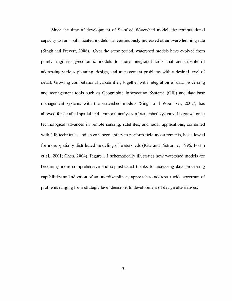
et al., 2001; Chen, 2004). Figure 1.1 schematically illustrates how watershed models are
becoming more comprehensive and sophisticated thanks to increasing data processing
capabilities and adoption of an interdisciplinary approach to address a wide spectrum of
problems ranging from strategic level decisions to development of design alternatives.
6
Figure 1.1.Integrated watershed modeling evolution over time.
Although the inherent complexity of water resources systems, coupled with lack of
data and insufficient computational capacities, has often led to artificial
compartmentalization of natural processes and human behavior for ease of modeling, the
last few decades have seen a marked shift towards multi-disciplinary and integrated
systems modeling (Estes, 1993; MacKenzie, 1996; Schultz, 2001; Madani and Mariño,
2009; Simonovic, 2009). The gradual shift from merely employing engineering-based
simulation models to applying integrated hydroeconomic models, and more recently
multi-criteria/multi-objective decision making and conflict resolution models, is an
indicator of promising changes in the traditional paradigm for the application of water
7
resources models. More holistic understanding of watershed systems, consideration of
multiple stakeholder values, objectives and behavior, and improved abilities to predict
and plan for future impacts are likely to lead to more sustainable water resources
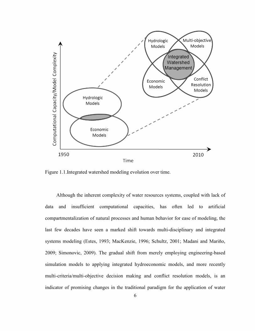
planning and management decisions. Figure 1.2 depicts the chronological evolution of
water resources planning and management approaches.
Figure 1.2.Chronological evolution of water resources planning and management
approaches (Adapted from Arshady, 2010).
8
1.3. Water resources modeling methods and approaches
Water resources modeling methods and approaches have been categorized in
different ways according to the types of problems they address and their method of
finding a preferred solution. When categorized according to their solution method,
models are classified either as simulation or optimization models. While there is a clear
distinction between these two, as will be described below, many water resources studies
involve a combination of simulation and optimization to analyze watershed systems and
develop effective management policies. Alternatively, water resources models may be
classified according to their scope and purpose into the following categories:
engineering-based watershed process models, hydroeconomic models, multi-criteria
(multi-objective) decision making models, and conflict resolution models. Each of these
categories of models is briefly described below.
1.3.1. Modeling methods: Simulation and optimization
There are some key differences in the philosophy of these two modeling methods,
and proper understanding of these differences is crucial to selection and application of the
appropriate model. Depending upon the type and nature of the water resources planning
and management problem being addressed, modelers have used either simulation or
optimization models as the primary methods to study and analyze watersheds. However,
optimization and simulation modeling are not mutually exclusive. In many studies, they
are used in complementary fashion to support decision making. For example, following
the preliminary screening of alternatives, feasible alternatives generated by optimization
9
can be simulated for detailed analysis and impact prediction (Loucks and van Beek,
2005).
Simulation models take physical parameters and engineered designs, or
management plans, as inputs and generate detailed predictions of outcomes. Simulation is
widely applied in the detailed design phase of projects for quantitative performance and
impact analysis of a limited number of alternative designs. The method is suitable for
sensitivity (or “what if”) analysis under a number of scenarios of interest. For example, a
modeler may wish to use a simulation model to evaluate the performance of alternative
designs under drought, normal, and flood scenarios. If performance of each alternative is
unacceptable, new alternatives must be developed and evaluated. Engineering-based
simulation is thus considered as an alternative-focused method in which the modeler
intends to reach the best possible alternative design or quantitative representation of
natural systems through a trial and error process (Makowski et. al., 1996; Garbrecht,
2006).
Optimization methods are geared towards creating alternatives based on selecting
values for decision variables that provide the best value of an objective function, subject
to a set of mathematical constraints (equations or limits that need to be satisfied in order
for a particular alternative to be feasible). Understandably, expressing operational
objectives and constraints in a mathematical form that can be solved by a computer often
requires simplification of physical and socioeconomic relationships. Some advantages of
optimization models are that they can help to screen a large number of potential
alternatives, generate new alternatives that otherwise may have been overlooked, and
provide an intuitive means of trade-off analysis. Also, optimization results need to be
10
interpreted carefully, as the “optimal” outcomes may be overly optimistic and not
achievable in practice. Table 1.1 compares some main aspects of simulation and
optimization models.
Table 1.1.Simulation versus optimization.
Modeling method Simulation Optimization
Key question addressed What if? What’s best?
Development effort Low High
Computational efficiency High Low
Transparency/ acceptability to the stakeholders High Low
1.3.2. Modeling approaches: Scope and problems addressed
1.3.2.1. Watershed process models
Watershed process simulation models are used for quantitative analysis, or
prediction, of natural processes occurring at the watershed scale, to understand
watersheds’ natural behavior or their response to human- engineered alterations (Singh
and Woolhiser, 2002). The structure of watershed process models varies depending upon
modeling objectives, but in general they are built using a series of mathematical
equations that describe the components of hydrologic or biogeochemical cycles, such as
surface water hydrology, hydrogeology, soil chemistry, and limnological processes, to
name a few. Presently, there exists a large number of generalized watershed simulation
models that include, among others, rainfall-runoff processes, river hydraulics,
groundwater hydraulics, and water quality processes (Wurbs, 1998). By focusing on
11
natural processes, these models are often able to provide a detailed representation of one
or more watershed subsystems. Engineering-based watershed process models are
frequently applied in watershed planning and management to help raise the decision
makers’ awareness of technical nuances of proposed design alternatives, and predict the
potential impacts of projects prior to their implementation. Watershed process models
have been used in a wide range of studies, including rainfall-runoff prediction, flood
mitigation design, water supply development, safety assessment of water infrastructure,
land use planning, irrigation planning, hydropower operations, and surface and
groundwater quality protection.
1.3.2.2. Hydroeconomic models
Apart from its life-sustaining role, water has economic value for various in-stream
and off-stream uses such as domestic use, agriculture, industry, transportation, recreation,
waste assimilation, and ecosystem maintenance (Gibbons, 1986). While physically-based
watershed process models can capture the natural hydrologic behavior of watersheds,
they have traditionally neglected the economic aspect of watershed modeling. However,
water scarcity manifested by drought-induced economic downturn and intensified by
growing demands for water necessitates consideration of appropriate economic factors in
a robust watershed modeling framework to devise economically justifiable watershed
management plans. Hydroeconomic models, often based on optimization methods,
possess the advantage of facilitating economic studies by maximizing or minimizing
some specified economic objective function subject to a series of constraints.
12
Harou et al. (2009) describe hydroeconomic models as solution-oriented tools that
foster formulation of new strategies to promote water-use efficiency and transparency of
decision making, thus contributing to integrated water resources management. However,
maximizing the economic value of water use serves as the only driver of decisions in
hydroeconomic models as economic valuation of many social, political and
environmental objectives remains difficult. Integrated modeling of watershed-scale
hydrological, environmental, and economic aspects of water use often requires simplified
representation of natural processes (Heinz et al., 2007). Thus, water resources
management decisions which are solely based on hydroeconomic models may not be
comprehensive and a holistic model and approach is required for integrated water
resources management. Hydroeconomic models have been applied to analyze water
resources management practices and potential economic and environmental impacts, to
address trade-offs and interactions among various stakeholder groups, to evaluate long
term drought management and flood mitigation plans, to improve water resources
operation policies and strategies, to suggest climate change adaptation strategies, and to
identify economically promising resources for environmental restoration (i.e., to improve
water quality and quantity for ecosystems).
1.3.2.3. Multi-objective decision making models
Water resources planning and management decisions must almost always consider
multiple goals, many of which are conflicting. Often it is impossible to aggregate the
goals into a single criterion or performance measure in the alternative ranking and
13
selection process (Makowski et. al., 1996). Thus, multi-criteria (or multi-objective)
decision support methods are widely applied for water policy planning and evaluation, as
well as infrastructure development (Hajkowicz and Collins, 2007). In the context of
optimization modeling, these methods seek to generate solutions that are “non-
dominated,” meaning that performance with respect to one objective cannot be improved
without decreasing performance with respect to another objective. For example, reservoir
operators need to consider the trade-off between water supply and flood mitigation
benefits, as increasing the reliability of meeting a target supply (i.e., storing more water
in a reservoir) would impose additional flood risk. By using optimization, all dominated
solutions may be screened out, and the non-dominated solutions evaluated for trade-offs,
allowing the decision maker to focus on a smaller set of potentially preferred alternatives
(Hajkowicz and Collins, 2007). For water resources systems, MCDM methods may
consider quantitative and qualitative criteria such as engineering standards and expected
performance, environmental integrity, investment and operating costs, equity, and
aesthetics (Hipel, 1992).
1.3.2.4. Conflict resolution models
The multitude of watershed planning and management objectives inevitably leads to
conflicts among watershed stakeholders, or interest groups. In many cases, however,
different stakeholder groups share common interests (e.g., a homeowner along a river
may be primarily concerned about flood risk reduction but may also value the riverine
ecosystem), or they may be able to reach compromise agreements (e.g., development of
14
one portion of the floodplain may be offset by enhancing wetlands in another portion).
Conflict resolution models essentially seek to promote compromise through holistic
understanding of technical, socioeconomic, political, and environmental aspects of the
problem (Lund and Palmer, 1997). Conflict resolution models have served as flexible
tools for quantitative and qualitative analysis of watershed systems to suggest, given the
circumstances, what would happen to the system based on detectable trends,
stakeholders’ interests, concerns, and behavior. Unlike the traditional “win-lose” or
“zero-sum” conflict resolution approach, water resources conflict resolution models seek
to lead the parties involved in the conflict towards a “win-win” situation or a “ positive-
sum”, socially feasible solution (Nandalal and Simonovic, 2003).
Conventionally, most multi-criteria decision making models tend to transform
multi-objective problems to a single composite objective (e.g. economic benefit,
environmental integrity, social welfare), assuming that stakeholders will perfectly
cooperate to reach the system’s optimal solution (Madani, 2009). However, such an
assumption may result in unrealistic results. Therefore, other conflict resolution models
such as game theory models have been used in water resources management, which are
capable of generating a more realistic simulation of stakeholders’ and decision makers’
behaviors by accounting for their concern to maximize their own benefit (Madani, 2010).
By creating a platform for collaborative modeling and constructive negotiation, conflict
resolution models can enhance stakeholders’ and decision makers’ understanding of the
problem and aid in the definition of solution objectives and constraints. Collaborative
modeling can facilitate the development of feasible alternatives, as well as the evaluation
of alternatives’ performance and impacts. Proper use of conflict resolution models has
15
been found to increase technical confidence in the solution agreed upon (Lund and
Palmer, 1997).
1.4. Objectives and organization
Water resources systems may be considered as hotspots for the sustainability
process as they lie at the intersection of socioeconomic and environmental subsystems.
As the need for comprehensive and reliable understanding of the consequences of natural
and anthropogenic alteration of watersheds has grown, so has interest in water resources
systems modeling to facilitate well-informed planning, and provide insights for decision
making. This dissertation will contribute to application of a quant-qualitative framework
for sustainable water resources management. It will focus on fundamentals of the systems
approach to holistic water resources management with application to water quality
management planning. Systems thinking and system dynamics simulation, as well as
environmental systems analysis techniques are applied to provide insights for water
quality management of example cases in the Great Lakes basin. The objectives of the
dissertation are as follows:
Illustrate the role of systems thinking paradigm in water resources planning and
decision making;
Demonstrate qualitative, as well as quantitative capabilities of system dynamics
modeling in facilitating holistic water resources modeling and policy making;
Identify and simulate the system structure driving the long-term eutrophication-
recovery trend of Lake Allegan, Michigan to provide insights into policy
leverages for mitigating impairment;
16
Develop a framework for applying the systems approach for implementation of
the concept of total maximum daily load (TMDL) for reducing non-point source
(NPS) total phosphorus (TP) emission in the Kalamazoo River watershed,
Michigan;
Investigate market-based policy options for mitigating total phosphorus loads in
the Maumee Basin.
This dissertation is organized in six chapters. The first chapter, as was presented in
the preceding sections, provides an introduction, giving background information about
how water resources models have become more holistic over the last decades. The
fundamentals of systems thinking and system dynamics as a suitable framework for
integrated analysis of water resources problems are discussed in Chapter 2. Furthermore,
an application of the systems approach to a water quality management problem is
presented in Chapter 3. The fourth and fifth chapters of the dissertation are devoted to
insights from application of the systems approach to water quality policy in the Great
Lakes Region. A simulation-optimization framework for guiding total maximum daily
load (TMDL) implementation in the Kalamazoo River watershed is presented in Chapter
4. Chapter 5 investigates a number of policy instruments for reducing TP loads in the
Maumee Basin, which covers parts of the three states of Indiana, Michigan, and Ohio.
The conclusions and potential areas of future research are given in Chapter 6.
17
1.5. References
Arshady, M. (2010). A systemic analysis of hydro energy and agriculture sectors’
vulnerability to water scarcity in the Great Karoon Basin. M.Sc. Thesis,
Department of Water Resources Engineering, Faculty of Agriculture, Tarbiat
Modares University, Tehran, Iran. In Persian.
Bagheri, A. (2006). Sustainable development: implementation in urban water systems.
Dissertation, Lund University, Lund, Sweden
<http://luur.lub.lu.se/luur?func=downloadFile&fileOId=546537> (accessed Oct.
22, 2009).
Beck, M.B., Fath, B.D., Parker, A.K., Osidele, O.O., Cowie, G.M., Rasmussen, T.C.,
Patten, .C., Norton, B.G., Steinmann, A., Borrett, S.R., Cox, D., Mayhew, M.C.,
Zeng, X.-Q., Zeng, W. (2002). Developing a concept of adaptive community
learning: case study of a rapidly urbanizing watershed. Integrated Assessment 3
(4), 299-307.
Brouwer, R., Hofkes M. (2008). Integrated hydro-economic modelling: approaches, key
issues and future research directions. Ecological Economics 66, 16-22.
Cai, X., McKinney, D. C., Lasdon, L. S. (2003). Integrated hydrologic-agronomic-
economic model for river basin management. Journal of Water Resource
Planning and Management 129, 4-17.
Chen, Y.D. (2004). Watershed modeling: where are we heading? Environmental
Informatics Archives 2, 132-139.
Crawford, N. H., Burges, S. J. (2004). History of the Stanford watershed model. Water
Resources Impact 6, 3–5.
18
Crawford, N.H., Linsley, R.K. (1966). Digital simulation in hydrology: Stanford
Watershed Model IV. Technical report No. 39, Department of Civil Engineering,
Stanford University, p. 210.
Fortin, J. P., Turcotte, R., Massicotte, S., Moussa, R., Fitzback, J., and Villeneuve, J. P.
(2001). A distributed watershed model compatible with remote sensing and GIS
data. I: Description of model. Journal of Hydrologic Engineering 6 (2), 91–99.
Freeze, R. A., Harlan, R. L. (1969). Blueprint for a physically-based, digitally-simulated
hydrologic response model. Journal of Hydrology 9, 237-258.
Garbrecht, J. D. (2006). Comparison of three alternative ANN designs for monthly
rainfall–runoff simulation. Journal of Hydrological Engineering 11, 502–505.
Gibbons, D.C. (1986). The Economic Value of Water. Resources for the Future,
Washington, D.C.
Hajkowicz S, Collins, K. (2007). A review of multiple criteria analysis for water
resources planning and management. Water Resources Management 21, 1553–
1566.
Harou, J.J., Pulido-Velazquez, M.A., Rosenberg, D.E., Medellin-Azuara, J., Lund, J.R.,
Howitt, R. (2009). Hydro-economic models: concepts, design, applications and
future prospects. Journal of Hydrology 375, 334-350.
Heinz, I., Pulido-Velasquez, M., Lund, J., Andreu, J. (2007). Hydro-economic modeling
in river basin management: implications and applications for the European Water
Framework Directive. Water Resources Management 21, 1103–1125.
Hipel, K. W. (1992). Multiple objective decision making in water resources. Water
Resources Bulletin 28, 3-12.
19
Johanson, R. C., Imhoff, J. C., Kittle, J. L., Donigian, A. S. (1984). Hydrologic
Simulation Program - FORTRAN (HSPF). User’s manual for release 8. Report
No. EPA-600/3- 84-066, U.S. EPA Environmental Research Lab, Athens, GA.
Kite, G. W., Pietrorino, A. (1996). Remote sensing applications in hydrological
modelling. Hydrological Sciences Journal 41(4), 563– 587.
Korfmacher, K.S. (2001). The politics of participation in watershed modeling.
Environmental Management 27(2), 161–176.
Langler, G.J., Smith, C. (2001). Effects of habitat enhancement on 0-group fishes in a
lowland river. Regulated Rivers: Research and Management 17, 677–686.
Loucks, D.P., van Beek, E. (2005). Water resources systems planning and management:
an introduction to methods, models and applications. In: Studies and reports in
hydrology. UNESCO Publishing, Paris.
Lund, J.R., Palmer, R.N. (1997). Water resource system modeling for conflict resolution.
Water Resources Update 108, 70-82.
Maass, A., Hufschmidt, M. A., Dorfman, R., Thomas, Jr., H. A., Marglin, S. A., Fair, G.
M. (1962). Design of water-resource systems: New techniques for relating
economic objectives, engineering analysis, and governmental planning. Harvard
University Press, Cambridge, Massachusetts.
Madani, K. (2009). Climate change effects on high-elevation hydropower system in
California. Ph.D. Dissertation, Department of Civil and Environmental
Engineering, University of California, Davis.
<http://cee.engr.ucdavis.edu/faculty/lund/students/ MadaniDissertation.pdf>
(accessed Nov.15, 2009).
20
Madani, K. (2010). Game theory and water resources. Journal of Hydrology 381(3-4),
225- 238.
Madani, K., Hipel, K. W. (2007). Strategic Insights into the Jordan River Conflict.
Proceeding of the 2007 World Environmental and Water Resources Congress,
Tampa, Florida, Edited by Kabbes K. C., pp. 1-10, American Society of Civil
Engineers, doi: 10.1061/40927(243)213.
Madani, K., Mariño, M.A. (2009). System dynamics analysis for managing Iran’s
Zayandeh-Rud River basin. Water Resources Management 23(11), 2163-2187.
Makowski, M., Somlyody, L., Watkins, D. (1996). Multiple criteria analysis for water
quality management in the Nitra Basin. Water Resources Bulletin 32, 937–947.
Nandalal , K.D.W. , Simonovic, S. P. (2003). State-of-the-art report on systems analysis
methods for resolution of conflicts in water resources management. UNESCO-
IHP Publication, PCCP Series, p. 20.
Reuss, M. (2003). Is it time to resurrect the Harvard Water Program? Journal of Water
Resources Planning and Management 129, 357-360.
Singh, V.P., Frevert, D.K., eds. (2006). Watershed Models. CRC Press, Boca Raton,
Florida.
Singh, V. P., Woolhiser, D. A. (2002). Mathematical modeling of watershed hydrology.
Journal of Hydrological Engineering 7(4), 270-292.
Tullos, D. (2009). Assessing the influence of environmental impact assessments on
science and policy: An analysis of the Three Gorges Project. Journal of
Environmental Management 90(Sup. 3), 208–223.
21
U.S. Army Corps of Engineers (1989). Water Control Software: Forecast and Operations.
Hydrologic Engineering Center, Davis, CA.
Wright, S.A., Schoellhamer, D.H. (2004). Trends in the sediment yield of the Sacramento
River, California, 1957–2001. San Francisco Estuary and Watershed Science (on
line serial), 2(2). <http://repositories.cdlib.org/jmie/sfews/vol2/iss2/art2/>
(accessed Oct.15, 2009).
Wurbs, R. A. (1998). Dissemination of generalized water resources models in the United
States. Water International 23, 190–198.
Wurbs, R.A., James, W.P. (2002). Water resources engineering. Prentice-Hall.NJ.
Yoshinobu, K., Tomohisa, Y., Toshimasa, H., Sadahiro, Y., Koji, I. (2006). Causes of
farmland salinization and remedial measures in the Aral Sea basin-Research on
water management to prevent secondary salinization in rice-based cropping
system in arid land. Agricultural Water Management 85, 1–14.
22
Chapter 2- Synthesis of system dynamics tools for holistic
conceptualization of water resources problems2
2.1. Abstract
Out-of-context analysis of water resources systems can result in unsustainable
management strategies. To address this problem, systems thinking seeks to understand
interactions among the subsystems driving a system’s overall behavior. System
dynamics, a method for operationalizing systems thinking, facilitates holistic
understanding of water resources systems, and strategic decision making. The approach
also facilitates participatory modeling, and analysis of the system’s behavioral trends,
essential to sustainable management. The field of water resources has not utilized the full
capacity of system dynamics in the thinking phase of integrated water resources studies.
This chapter advocates that the thinking phase of modeling applications is critically
important, and that system dynamics offers unique qualitative tools that improve
understanding of complex problems. Thus, this chapter describes the utility of system
dynamics for holistic water resources planning and management by illustrating the
fundamentals of the approach. Using tangible examples, the chapter provides an
overview of Causal Loop and Stock and Flow Diagrams, reference modes of dynamic
2 This chapter is a reprint of the article: Mirchi, A., Madani, K., Watkins, D.W. Jr., Ahmad, S., (2012).
Synthesis of system dynamics tools for holistic conceptualization of water resources problems. Water
Resources Management 26(9), 2421-2442. Reprinted with permission from Springer.
23
behavior, and system archetypes to demonstrate the use of these qualitative tools for
holistic conceptualization of water resources problems. Finally, the chapter presents a
summary of the potential benefits as well as caveats of qualitative system dynamics for
water resources decision making.
2.2. Introduction
An event-oriented view of the world or linear causal thinking cannot address
complex problems adequately (Forrester, 1961 and 1969; Richmond, 1993; Sterman,
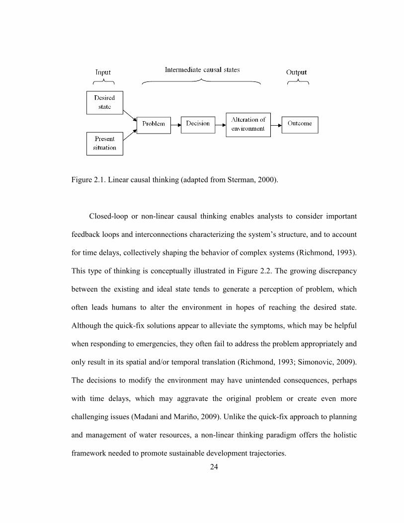
2000). Figure 2.1 illustrates this unidirectional thinking paradigm, which is grounded on
the intuitive assumption that outputs or events are shaped by the collective effect of a
series of inputs or causes acting sequentially (Sterman, 2000). One artifact of this type of
thinking is that many problems, manifested by discrepancies between the present state
and an expected or desired state, are singled out and treated in isolation from the
surrounding environment. Consequently, no in-depth understanding of root causes of
problems is obtained. Thus, managing complex water resources systems using uni-
directional, mechanistic models may be doomed to provide unrealistic, or at least,
questionable results (Hjorth and Bagheri, 2006).
24
Figure 2.1. Linear causal thinking (adapted from Sterman, 2000).
Closed-loop or non-linear causal thinking enables analysts to consider important
feedback loops and interconnections characterizing the system’s structure, and to account
for time delays, collectively shaping the behavior of complex systems (Richmond, 1993).
This type of thinking is conceptually illustrated in Figure 2.2. The growing discrepancy
between the existing and ideal state tends to generate a perception of problem, which
often leads humans to alter the environment in hopes of reaching the desired state.
Although the quick-fix solutions appear to alleviate the symptoms, which may be helpful
when responding to emergencies, they often fail to address the problem appropriately and
only result in its spatial and/or temporal translation (Richmond, 1993; Simonovic, 2009).
The decisions to modify the environment may have unintended consequences, perhaps
with time delays, which may aggravate the original problem or create even more
challenging issues (Madani and Mariño, 2009). Unlike the quick-fix approach to planning
and management of water resources, a non-linear thinking paradigm offers the holistic
framework needed to promote sustainable development trajectories.
25
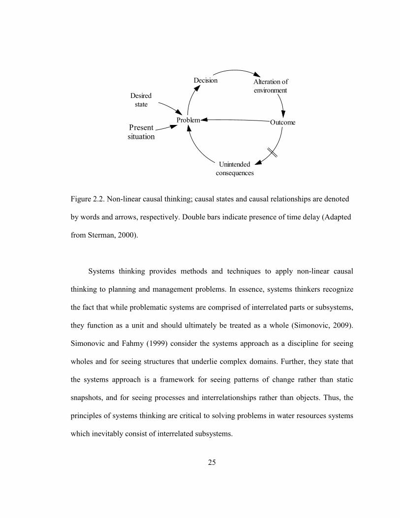
Figure 2.2. Non-linear causal thinking; causal states and causal relationships are denoted
by words and arrows, respectively. Double bars indicate presence of time delay (Adapted
from Sterman, 2000).
Systems thinking provides methods and techniques to apply non-linear causal
thinking to planning and management problems. In essence, systems thinkers recognize
the fact that while problematic systems are comprised of interrelated parts or subsystems,
they function as a unit and should ultimately be treated as a whole (Simonovic, 2009).
Simonovic and Fahmy (1999) consider the systems approach as a discipline for seeing
wholes and for seeing structures that underlie complex domains. Further, they state that
the systems approach is a framework for seeing patterns of change rather than static
snapshots, and for seeing processes and interrelationships rather than objects. Thus, the
principles of systems thinking are critical to solving problems in water resources systems
which inevitably consist of interrelated subsystems.
Desiredstate
Presentsituation
Problem
Decision Alteration ofenvironment
Outcome
Unintendedconsequences
26
System dynamics (Forrester, 1961 and 1969; Meadows, 1972; Richmond, 1993;
Ford, 1999; Sterman, 2000) is one of the methods that facilitate recognition of
interactions among disparate but interconnected subsystems driving the system’s
dynamic behavior. The method can thus help water resources analysts to identify
problematic trends and comprehend their root causes in a holistic fashion. By identifying
and capturing feedback loops between components, system dynamics models can provide
insights into potential consequences of system perturbations, thereby serving as a suitable
platform for sustainable water resources planning and management at the strategic level
(Hjorth and Bagheri, 2006; Madani and Mariño, 2009; Simonovic, 2009). To this end,
system dynamics offers several qualitative and quantitative tools to identify and explain
system behavior over time.
System dynamics has not been used by most water resources scholars and
practitioners to its full capacity. The majority of system dynamics applications in water
resources have underutilized the method’s qualitative modeling tools. The
conceptualization or thinking phase of integrated water resources studies is of paramount
importance as it provides fundamental understanding of leverage points for sustainable
solutions. High level and qualitative models can be developed relatively quickly and
affordably to facilitate trend identification, and to provide insights into root causes of
multi-faceted water resources problems, facilitating formulation of preemptive and
sustainable solution strategies. This chapter provides a synthesis of qualitative modeling
techniques offered by system dynamics and argue that these techniques offer important
insights and should not be overlooked by water resource modelers. To do this, the chapter
first presents a synopsis of system dynamics applications in water resources. Then, the
27
fundamentals of system dynamics and its qualitative modeling tools such as Causal Loop
Diagrams (CLD) and Stock and Flow Diagrams (SFD) are discussed in detail, using
tangible examples to illustrate why this approach is well suited for integrated water
resources modeling, planning, and management. Furthermore, reference modes of
dynamic behavior and merits of using system archetypes for qualitative modeling prior to
quantitative analyses are illustrated. Finally, the method’s benefits and caveats, stemming
from application of the approach without proper regard for its philosophy, are discussed.
2.3. System dynamics and water resources
System dynamics, a sub-field of systems thinking (Richmond, 1994; Ford, 1999),
originated in the 1960’s when the concepts of feedback theory were applied by Forrester
and his colleagues to understand the underlying structure and dynamics of industrial and
urban systems (Forrester, 1961 and 1969). The method has since been widely used by
analysts from various disciplines as a convenient tool to explore the causal relationships
forming feedback loops between different components of large systems. In the past 50
years, system dynamics has become a well-established methodology that has been
applied in many different practical and scientific fields, including management, ecology,
economics, education, engineering, public health, and sociology (Sterman, 2000).
Application of system dynamics in water resources engineering and management
has grown over the past two decades (Winz et al., 2009). Reviewing the literature, three
general approaches to water resources system dynamics modeling can be identified: (i)
predictive simulation models; (ii) descriptive integrated models; and (iii) participatory
28
and shared vision models. In the first class of system dynamics models, modelers have
successfully used the method as a tool to quantitatively simulate the processes governing
particular subsystems within a broader water resources system. For example, Ahmad and
Simonovic (2000) used system dynamics to model the interactive components of the
hydrologic cycle to develop reservoir operation rules for flood mitigation. Ideally, this
type of system dynamics model is developed to help predict the future behavior of the
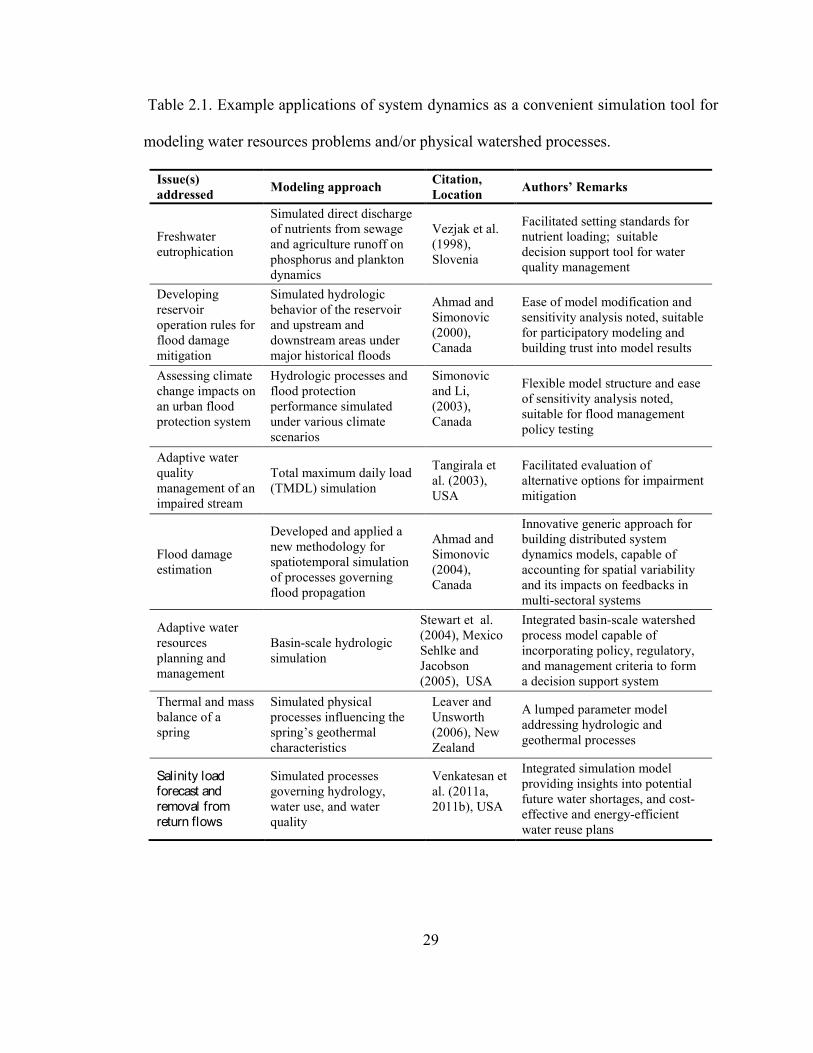
system accurately enough to provide a basis for tactical decisions. Table 2.1 presents
some examples of water resources problems addressed using system dynamics as a
convenient simulation tool for analyzing water resources problems and/or physical
watershed processes.
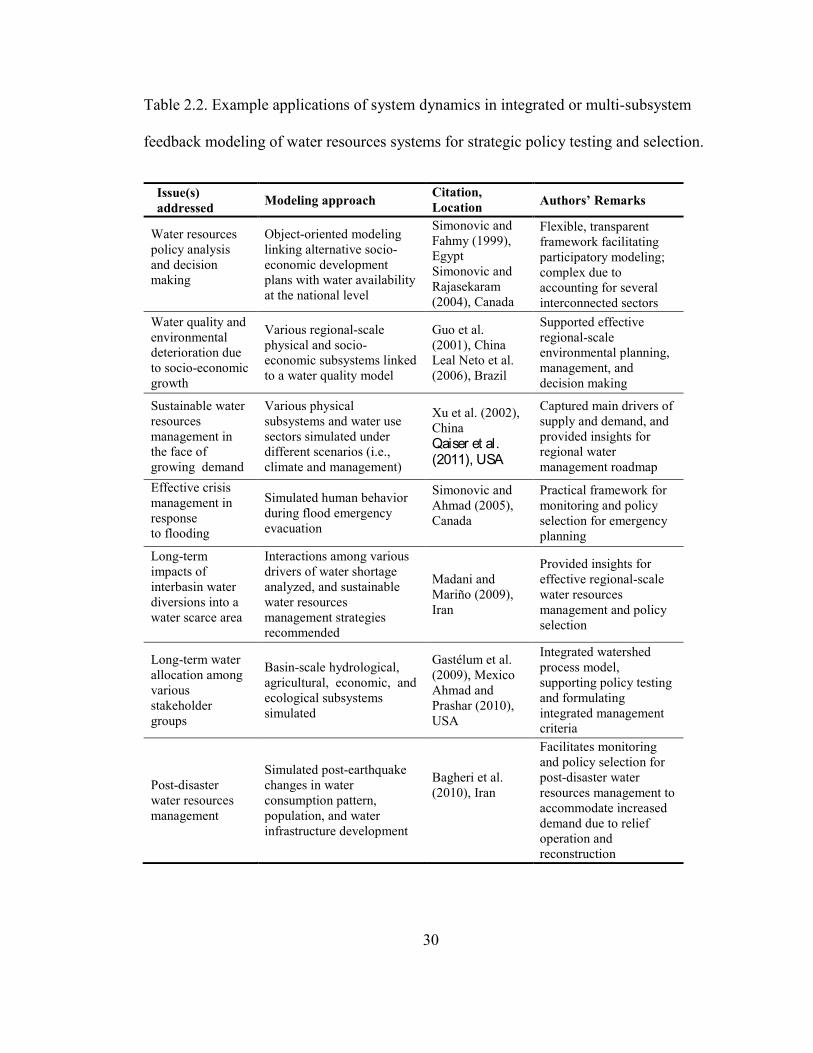
In the second class of system dynamics models, analysts have adopted a more
holistic approach, striving to identify and characterize the main feedback loops among
two or more disparate subsystems, such as hydrological, ecological, environmental,
socio-economic, and political subsystems. Typically, these integrated feedback models
facilitate testing and selection of water resources management plans and policies at the
strategic level. Table 2.2 summarizes example water resources studies, which have used
system dynamics to describe and better understand the feedback structure and long-term
behavioral patterns of interacting water resources subsystems.
29
Table 2.1. Example applications of system dynamics as a convenient simulation tool for
modeling water resources problems and/or physical watershed processes.
Issue(s) addressed Modeling approach Citation,
Location Authors’ Remarks
Freshwater eutrophication
Simulated direct discharge of nutrients from sewage and agriculture runoff on phosphorus and plankton dynamics
Vezjak et al. (1998), Slovenia
Facilitated setting standards for nutrient loading; suitable decision support tool for water quality management
Developing reservoir operation rules for flood damage mitigation
Simulated hydrologic behavior of the reservoir and upstream and downstream areas under major historical floods
Ahmad and Simonovic (2000), Canada
Ease of model modification and sensitivity analysis noted, suitable for participatory modeling and building trust into model results
Assessing climate change impacts on an urban flood protection system
Hydrologic processes and flood protection performance simulated under various climate scenarios
Simonovic and Li, (2003), Canada
Flexible model structure and ease of sensitivity analysis noted, suitable for flood management policy testing
Adaptive water quality management of an impaired stream
Total maximum daily load (TMDL) simulation
Tangirala et al. (2003), USA
Facilitated evaluation of alternative options for impairment mitigation
Flood damage estimation
Developed and applied a new methodology for spatiotemporal simulation of processes governing flood propagation
Ahmad and Simonovic (2004), Canada
Innovative generic approach for building distributed system dynamics models, capable of accounting for spatial variability and its impacts on feedbacks in multi-sectoral systems
Adaptive water resources planning and management
Basin-scale hydrologic simulation
Stewart et al. (2004), Mexico Sehlke and Jacobson (2005), USA
Integrated basin-scale watershed process model capable of incorporating policy, regulatory, and management criteria to form a decision support system
Thermal and mass balance of a spring
Simulated physical processes influencing the spring’s geothermal characteristics
Leaver and Unsworth (2006), New Zealand
A lumped parameter model addressing hydrologic and geothermal processes
Salinity load forecast and removal from return flows
Simulated processes governing hydrology, water use, and water quality
Venkatesan et al. (2011a, 2011b), USA
Integrated simulation model providing insights into potential future water shortages, and cost-effective and energy-efficient water reuse plans
30
Table 2.2. Example applications of system dynamics in integrated or multi-subsystem
feedback modeling of water resources systems for strategic policy testing and selection.
Issue(s) addressed Modeling approach Citation,
Location
Authors’ Remarks
Water resources policy analysis and decision making
Object-oriented modeling linking alternative socio-economic development plans with water availability at the national level
Simonovic and Fahmy (1999), Egypt Simonovic and Rajasekaram (2004), Canada
Flexible, transparent framework facilitating participatory modeling; complex due to accounting for several interconnected sectors
Water quality and environmental deterioration due to socio-economic growth
Various regional-scale physical and socio-economic subsystems linked to a water quality model
Guo et al. (2001), China Leal Neto et al. (2006), Brazil
Supported effective regional-scale environmental planning, management, and decision making
Sustainable water resources management in the face of growing demand
Various physical subsystems and water use sectors simulated under different scenarios (i.e., climate and management)
Xu et al. (2002), China Qaiser et al. (2011), USA
Captured main drivers of supply and demand, and provided insights for regional water management roadmap
Effective crisis management in response to flooding
Simulated human behavior during flood emergency evacuation
Simonovic and Ahmad (2005), Canada
Practical framework for monitoring and policy selection for emergency planning
Long-term impacts of interbasin water diversions into a water scarce area
Interactions among various drivers of water shortage analyzed, and sustainable water resources management strategies recommended
Madani and Mariño (2009), Iran
Provided insights for effective regional-scale water resources management and policy selection
Long-term water allocation among various stakeholder groups
Basin-scale hydrological, agricultural, economic, and ecological subsystems simulated
Gastélum et al. (2009), Mexico Ahmad and Prashar (2010), USA
Integrated watershed process model, supporting policy testing and formulating integrated management criteria
Post-disaster water resources management
Simulated post-earthquake changes in water consumption pattern, population, and water infrastructure development
Bagheri et al. (2010), Iran
Facilitates monitoring and policy selection for post-disaster water resources management to accommodate increased demand due to relief operation and reconstruction
31
Additionally, system dynamics models have been used as practical tools for
promoting shared vision planning, participatory modeling, and shared learning
opportunities for diverse groups of decision makers and stakeholder groups (Werick and
Whipple, 1994; Lund and Palmer, 1997; Creighton and Langsdale, 2009). Stakeholders’
participation in a group model building activity can increase understanding of the scope
and complexity of the problem, increase trust in model results and, subsequently, increase
support for the selected policy (Stave, 2003; Tidwell et al., 2004). Table 2.3 presents
examples of participatory water resources modeling using system dynamics.
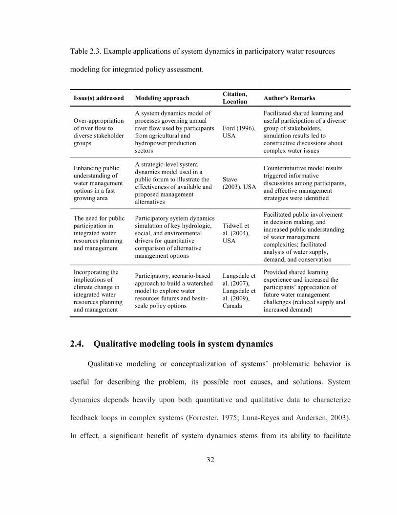
32
Table 2.3. Example applications of system dynamics in participatory water resources
modeling for integrated policy assessment.
Issue(s) addressed Modeling approach Citation, Location
Author’s Remarks
Over-appropriation of river flow to diverse stakeholder groups
A system dynamics model of processes governing annual river flow used by participants from agricultural and hydropower production sectors
Ford (1996), USA
Facilitated shared learning and useful participation of a diverse group of stakeholders, simulation results led to constructive discussions about complex water issues
Enhancing public understanding of water management options in a fast growing area
A strategic-level system dynamics model used in a public forum to illustrate the effectiveness of available and proposed management alternatives
Stave (2003), USA
Counterintuitive model results triggered informative discussions among participants, and effective management strategies were identified
The need for public participation in integrated water resources planning and management
Participatory system dynamics simulation of key hydrologic, social, and environmental drivers for quantitative comparison of alternative management options
Tidwell et al. (2004), USA
Facilitated public involvement in decision making, and increased public understanding of water management complexities; facilitated analysis of water supply, demand, and conservation
Incorporating the implications of climate change in integrated water resources planning and management
Participatory, scenario-based approach to build a watershed model to explore water resources futures and basin-scale policy options
Langsdale et al. (2007), Langsdale et al. (2009), Canada
Provided shared learning experience and increased the participants’ appreciation of future water management challenges (reduced supply and increased demand)
2.4. Qualitative modeling tools in system dynamics
Qualitative modeling or conceptualization of systems’ problematic behavior is
useful for describing the problem, its possible root causes, and solutions. System
dynamics depends heavily upon both quantitative and qualitative data to characterize
feedback loops in complex systems (Forrester, 1975; Luna-Reyes and Andersen, 2003).
In effect, a significant benefit of system dynamics stems from its ability to facilitate
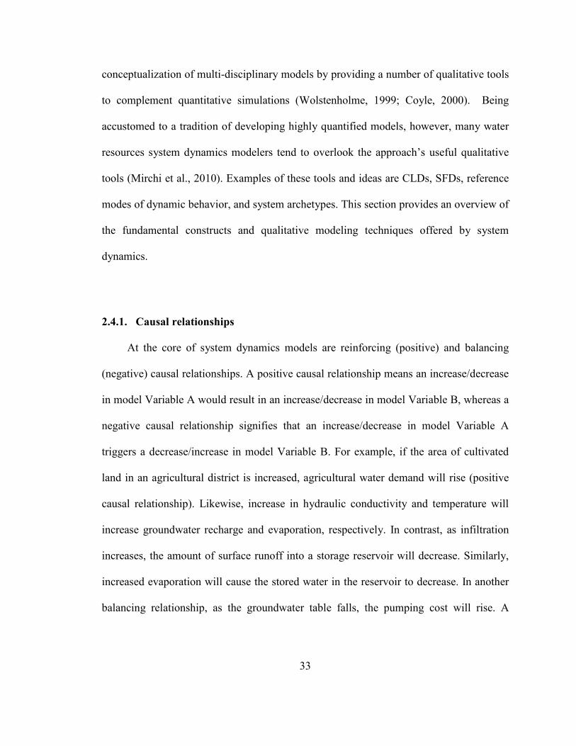
33
conceptualization of multi-disciplinary models by providing a number of qualitative tools
to complement quantitative simulations (Wolstenholme, 1999; Coyle, 2000). Being
accustomed to a tradition of developing highly quantified models, however, many water
resources system dynamics modelers tend to overlook the approach’s useful qualitative
tools (Mirchi et al., 2010). Examples of these tools and ideas are CLDs, SFDs, reference
modes of dynamic behavior, and system archetypes. This section provides an overview of
the fundamental constructs and qualitative modeling techniques offered by system
dynamics.
2.4.1. Causal relationships
At the core of system dynamics models are reinforcing (positive) and balancing
(negative) causal relationships. A positive causal relationship means an increase/decrease
in model Variable A would result in an increase/decrease in model Variable B, whereas a
negative causal relationship signifies that an increase/decrease in model Variable A
triggers a decrease/increase in model Variable B. For example, if the area of cultivated
land in an agricultural district is increased, agricultural water demand will rise (positive
causal relationship). Likewise, increase in hydraulic conductivity and temperature will
increase groundwater recharge and evaporation, respectively. In contrast, as infiltration
increases, the amount of surface runoff into a storage reservoir will decrease. Similarly,
increased evaporation will cause the stored water in the reservoir to decrease. In another
balancing relationship, as the groundwater table falls, the pumping cost will rise. A
34
A B+
A B-
summary of the given examples, along with graphical notation of reinforcing and
balancing causal relationships and their interpretation, is presented in Table 2.4.
Table 2.4. Graphical notation and polarity of causal relationships.
Connection Causal relationship Mathematical definition
Examples
Any change in the state of A causes the
state of B to change in the same direction; if
A increases/decreases, B increases/decreases
Any change in the state of A causes the
state of B to change in the opposite direction;
if A increases/decreases, B
decreases/increases
2.4.2. Causal loop diagrams and basic feedback loops
Developing the system’s CLD helps graphically capture the relationships between
interactive subsystems, and can thus be considered as the conceptual modeling step.
CLDs provide valuable information about the system including the presence of feedback
loops, loop dominance, and presence of time delays. They are comprised of words and
arrows with appropriate polarity, depicting combinations of positive and/or negative
causal relationships. A causal relationship may exist between any two system variables,
regardless of their type. In complex systems, combinations of positive and negative
causal relationships may form feedback loops. There are two fundamental feedback
Groundwater table
Evaporation
Infiltration
Pumping cost
Reservoir’s stored water
Runoff
Agricultural water demand Groundwater
recharge Evaporation
Cultivated land
Hydraulic conductivity Temperature
35
loops--balancing (negative) and reinforcing (positive) loops. Typically, a balancing
feedback loop comprises causal relationships which collectively attempt to reduce the
discrepancy between the current state and a desired state. On the other hand, reinforcing
feedback loops often characterize continuing trends of growth or decline. As a rule of
thumb, a loop is reinforcing if the number of its negative causal links is even, and it is
balancing otherwise, provided that the CLD appropriately represents the main drivers and
causal relationships between them (Sterman, 2000). The ability to observe the structure of
systems to identify dominant feedback loops in a representative CLD can provide
qualitative information about their typical dynamic behavior. Therefore, when systems
are not overly complex, it may be possible by looking at the CLD to determine the
behavior of some variables even before quantitative modeling. A simple example is used
to illustrate the behavior of reinforcing and balancing feedback loops, and the use of
CLDs in qualitative modeling.
To better understand the behavior of a reinforcing feedback loop, consider a
reservoir supplying water for a growing urban area. Net precipitation increases the
inflow, raising the reservoir’s stored water and increasing the potential for development
(positive relationships). Subsequently, new opportunities for development lead to actual
development, raising water demand, which then prompts the reservoir operators to
allocate more space in the reservoir to storage. Allocating more space to storage would
then create potential for more development which, in turn, would ultimately call for still
more stored water. In the absence of other operating feedbacks (e.g., flooding,
environmental flows, evaporation), the stored water in the system would grow
exponentially until storage capacity has completely been used. Figure 2.3 shows a simple
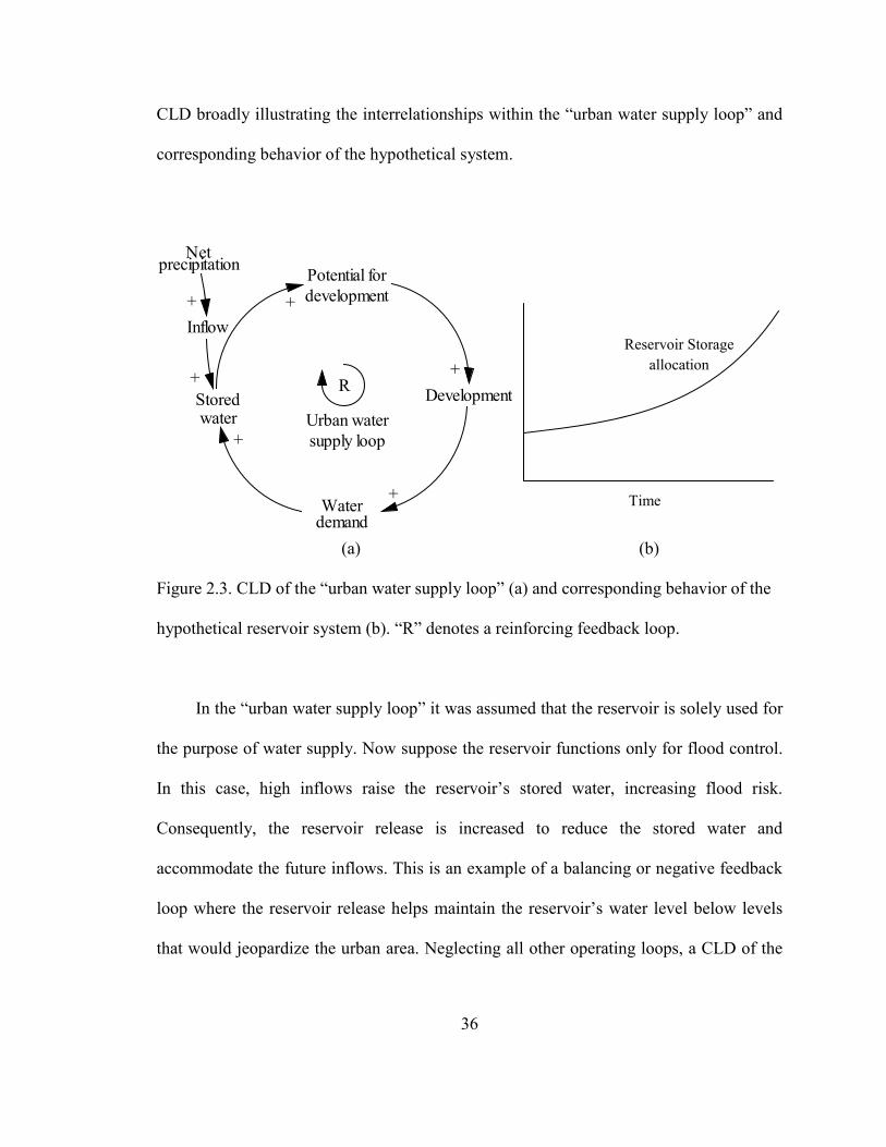
36
Netprecipitation
Inflow
Storedwater
Potential fordevelopment
Development
Waterdemand
+
+
+
+
+
+Urban watersupply loop
R
CLD broadly illustrating the interrelationships within the “urban water supply loop” and
corresponding behavior of the hypothetical system.
(a) (b)
Figure 2.3. CLD of the “urban water supply loop” (a) and corresponding behavior of the
hypothetical reservoir system (b). “R” denotes a reinforcing feedback loop.
In the “urban water supply loop” it was assumed that the reservoir is solely used for
the purpose of water supply. Now suppose the reservoir functions only for flood control.
In this case, high inflows raise the reservoir’s stored water, increasing flood risk.
Consequently, the reservoir release is increased to reduce the stored water and
accommodate the future inflows. This is an example of a balancing or negative feedback
loop where the reservoir release helps maintain the reservoir’s water level below levels
that would jeopardize the urban area. Neglecting all other operating loops, a CLD of the
Reservoir Storage allocation
Time
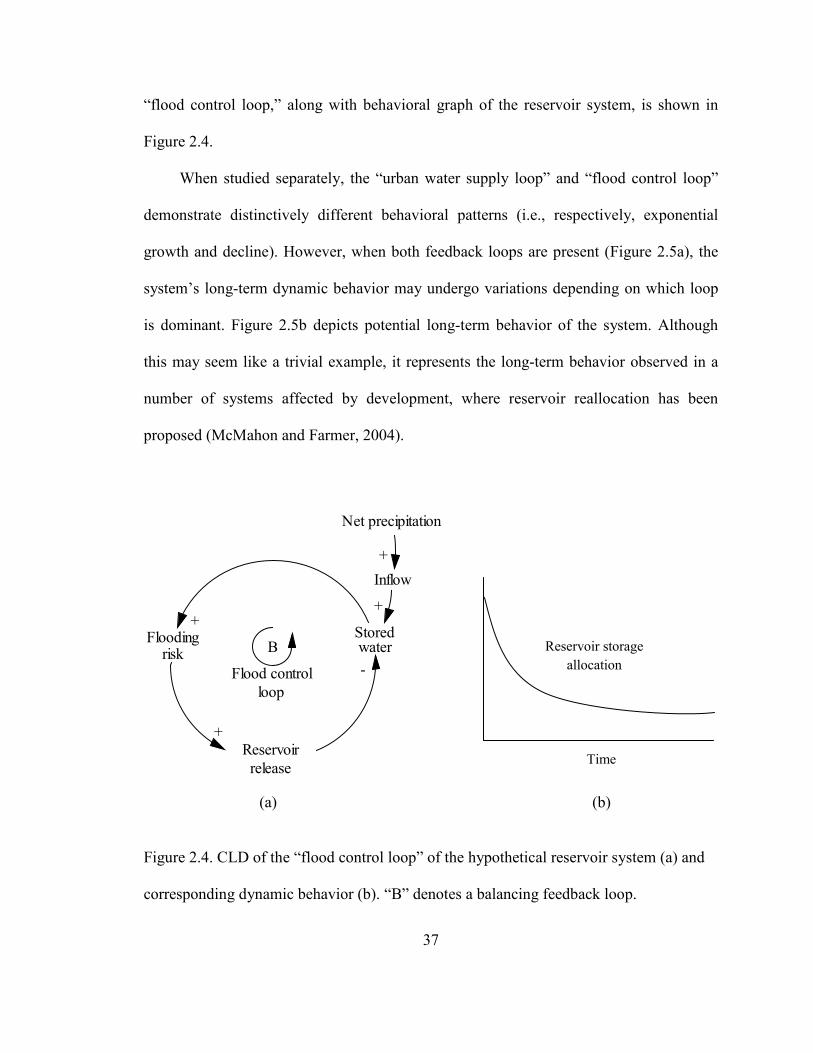
37
Storedwater
Net precipitation
Inflow+
+
Flood controlloop
Floodingrisk
Reservoirrelease
+
+
-B
“flood control loop,” along with behavioral graph of the reservoir system, is shown in
Figure 2.4.
When studied separately, the “urban water supply loop” and “flood control loop”
demonstrate distinctively different behavioral patterns (i.e., respectively, exponential
growth and decline). However, when both feedback loops are present (Figure 2.5a), the
system’s long-term dynamic behavior may undergo variations depending on which loop
is dominant. Figure 2.5b depicts potential long-term behavior of the system. Although
this may seem like a trivial example, it represents the long-term behavior observed in a
number of systems affected by development, where reservoir reallocation has been
proposed (McMahon and Farmer, 2004).
(a) (b)
Figure 2.4. CLD of the “flood control loop” of the hypothetical reservoir system (a) and
corresponding dynamic behavior (b). “B” denotes a balancing feedback loop.
Reservoir storage allocation
Time
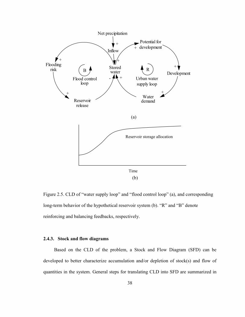
38
(a) (b)
Figure 2.5. CLD of “water supply loop” and “flood control loop” (a), and corresponding
long-term behavior of the hypothetical reservoir system (b). “R” and “B” denote
reinforcing and balancing feedbacks, respectively.
2.4.3. Stock and flow diagrams
Based on the CLD of the problem, a Stock and Flow Diagram (SFD) can be
developed to better characterize accumulation and/or depletion of stock(s) and flow of
quantities in the system. General steps for translating CLD into SFD are summarized in
Storedwater Development
R
Net precipitation
Inflow
+
Reservoirrelease
+ Potential fordevelopment
Waterdemand
Floodingrisk
+
+
+
+ Urban watersupply loop
Flood controlloop
+
+
-
B
Reservoir storage allocation
Time
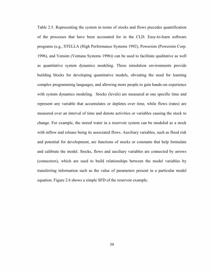
39
Table 2.5. Representing the system in terms of stocks and flows precedes quantification
of the processes that have been accounted for in the CLD. Easy-to-learn software
programs (e.g., STELLA (High Performance Systems 1992), Powersim (Powersim Corp.
1996), and Vensim (Ventana Systems 1996)) can be used to facilitate qualitative as well
as quantitative system dynamics modeling. These simulation environments provide
building blocks for developing quantitative models, obviating the need for learning
complex programming languages, and allowing more people to gain hands-on experience
with system dynamics modeling. Stocks (levels) are measured at one specific time and
represent any variable that accumulates or depletes over time, while flows (rates) are
measured over an interval of time and denote activities or variables causing the stock to
change. For example, the stored water in a reservoir system can be modeled as a stock
with inflow and release being its associated flows. Auxiliary variables, such as flood risk
and potential for development, are functions of stocks or constants that help formulate
and calibrate the model. Stocks, flows and auxiliary variables are connected by arrows
(connectors), which are used to build relationships between the model variables by
transferring information such as the value of parameters present in a particular model
equation. Figure 2.6 shows a simple SFD of the reservoir example.
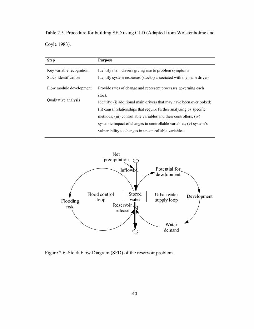
40
Table 2.5. Procedure for building SFD using CLD (Adapted from Wolstenholme and
Coyle 1983).
Step Purpose
Key variable recognition Identify main drivers giving rise to problem symptoms
Stock identification Identify system resources (stocks) associated with the main drivers
Flow module development Provide rates of change and represent processes governing each
stock Qualitative analysis Identify: (i) additional main drivers that may have been overlooked;
(ii) causal relationships that require further analyzing by specific
methods; (iii) controllable variables and their controllers; (iv)
systemic impact of changes to controllable variables; (v) system’s
vulnerability to changes in uncontrollable variables
Figure 2.6. Stock Flow Diagram (SFD) of the reservoir problem.
Netprecipitation
Potential fordevelopment
Development
Waterdemand
Floodingrisk
Storedwater
Inflow
Reservoirrelease
Flood controlloop
Urban watersupply loop
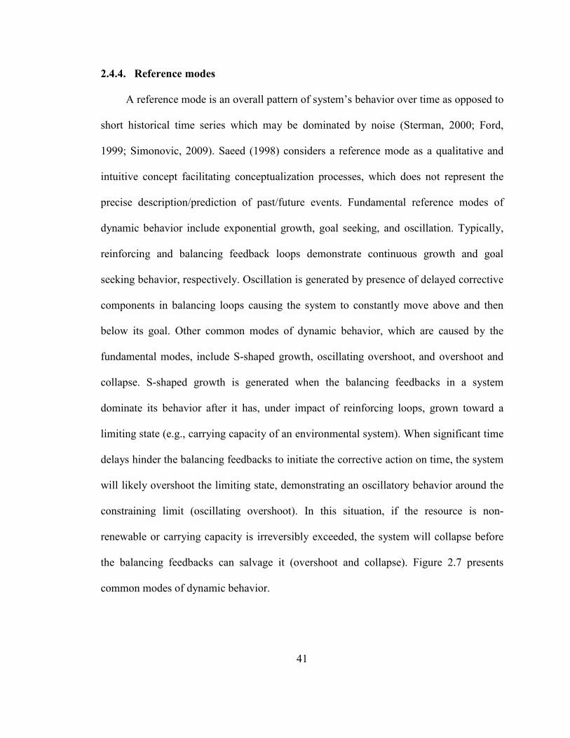
41
2.4.4. Reference modes
A reference mode is an overall pattern of system’s behavior over time as opposed to
short historical time series which may be dominated by noise (Sterman, 2000; Ford,
1999; Simonovic, 2009). Saeed (1998) considers a reference mode as a qualitative and
intuitive concept facilitating conceptualization processes, which does not represent the
precise description/prediction of past/future events. Fundamental reference modes of
dynamic behavior include exponential growth, goal seeking, and oscillation. Typically,
reinforcing and balancing feedback loops demonstrate continuous growth and goal
seeking behavior, respectively. Oscillation is generated by presence of delayed corrective
components in balancing loops causing the system to constantly move above and then
below its goal. Other common modes of dynamic behavior, which are caused by the
fundamental modes, include S-shaped growth, oscillating overshoot, and overshoot and
collapse. S-shaped growth is generated when the balancing feedbacks in a system
dominate its behavior after it has, under impact of reinforcing loops, grown toward a
limiting state (e.g., carrying capacity of an environmental system). When significant time
delays hinder the balancing feedbacks to initiate the corrective action on time, the system
will likely overshoot the limiting state, demonstrating an oscillatory behavior around the
constraining limit (oscillating overshoot). In this situation, if the resource is non-
renewable or carrying capacity is irreversibly exceeded, the system will collapse before
the balancing feedbacks can salvage it (overshoot and collapse). Figure 2.7 presents
common modes of dynamic behavior.
42
Figure 2.7. Common modes of dynamic behavior (Adapted from Sterman, 2000).
A water-stressed region’s ongoing trend of development, facilitated by continuous
supply of imported water, is an example of exponential growth driven by a reinforcing
feedback structure (Madani and Mariño, 2009). In contrast, irrigation water withdrawal in
an agricultural district where appropriate water pricing schemes are applied often follows
a goal seeking dynamic behavior (Cai and Wang, 2006). An example of oscillatory
dynamic behavior is a lake’s water level which fluctuates seasonally due to seasonal
precipitation patterns and water demands, and perhaps as mandated by lake operation
rules (e.g., Watkins and Moser, 2006). When water resources limit a region’s
development (i.e., no water can be supplied from outside the watershed), the water
consumption pattern will likely demonstrate S-shaped behavior (Bagheri and Hjorth,
2007). If long delays hinder timely response to warning signals (e.g., severe water stress),
43
the system may overshoot its limit, causing social, economic, and/or environmental
hardships. On the other hand, if the water resources are eventually replenished, it is likely
that continued growth and consumption will exhaust the newly available water,
generating alternating periods of replenishment and depletion, characterized by an
oscillating overshoot mode of dynamic behavior. In an extreme case, extensive
development in resource-stressed areas can completely exhaust the resources necessary
for survival of the system causing it to collapse (Erickson and Gowdy, 2000).
2.4.5. System archetypes
System archetypes are generic system structures showing common patterns of
behavior (Senge, 1990; Wolstenholme, 2003). Reinforcing and balancing feedback loops
are essentially the basic system archetypes. In real systems, however, a combination of
reinforcing and balancing feedback structures can form more complex dynamic behaviors
that can be characterized using more sophisticated system archetypes. Through closely
studying the structure of many systems, a number of archetypes have been identified that
can serve as diagnostic tools, describing or predicting the system’s long-run behavior.
Some common archetypes are Limits to Growth, Success to the Successful, Fixes that
Backfire, and Tragedy of the Commons (Senge, 1990). Knowledge of the governing
dynamics of water resources systems may help decision makers prognosticate
problematic behavior and take appropriate corrective actions in a timely fashion, leading
to more sustainable water resources planning and management. In this section, the
applicability of some system archetypes to characterize water resources management
problems is illustrated through a number of examples.
44
2.4.5.1. Limits to growth
The Limits to Growth archetype hypothesizes that continuous growth, driven by
reinforcing feedback loops in natural systems, will eventually push the system toward its
limit (e.g., carrying capacity). Once the system has grown beyond a critical level,
balancing feedback loops take over and dominate the system’s behavior, attempting to
prevent its collapse (Meadows, 1972). Dynamic behavior of an agricultural system using
groundwater as its source of irrigation water is an example of this archetype. A CLD of
the Limits to Growth archetype for the given agricultural system is depicted in Figure
2.8a. In this system, agricultural growth raises the demand of irrigation water. Farmers
may then develop additional groundwater resources and increase pumping, enhancing the
potential for agricultural growth and an increase in cultivated land (reinforcing loop).
However, pumping excessive amounts of groundwater will cause severe drawdown of the
groundwater table, increasing the pumping cost which, in turn, reduces the demand for
groundwater (balancing loop). As shown in Figure 2.8b, pumping cost increases with
continuous agricultural growth until groundwater withdrawal is no longer economical,
which then reduces the growth. In an extreme case, if a non-renewable groundwater
resource is completely exhausted, the agricultural practice may cease altogether.
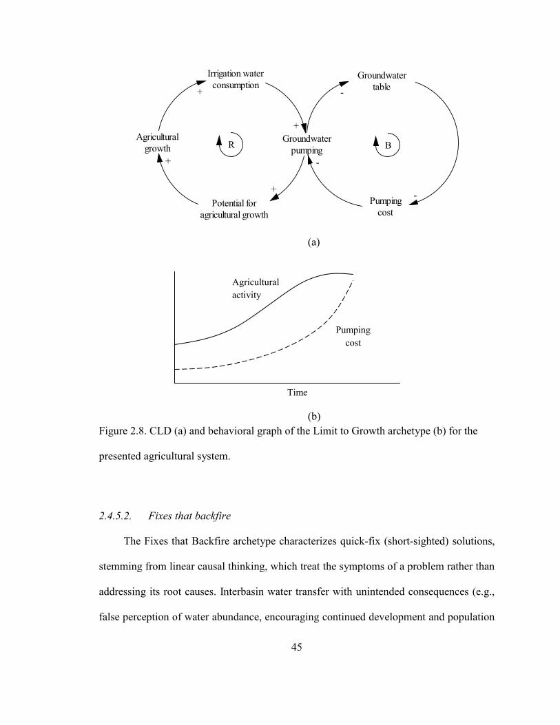
45
(a) (b) Figure 2.8. CLD (a) and behavioral graph of the Limit to Growth archetype (b) for the
presented agricultural system.
2.4.5.2. Fixes that backfire
The Fixes that Backfire archetype characterizes quick-fix (short-sighted) solutions,
stemming from linear causal thinking, which treat the symptoms of a problem rather than
addressing its root causes. Interbasin water transfer with unintended consequences (e.g.,
false perception of water abundance, encouraging continued development and population
Irrigation waterconsumption
Groundwaterpumping
Potential foragricultural growth
Agriculturalgrowth
Groundwatertable
Pumpingcost
+
+
+
+
-
-
-
R B
Time
Pumping cost
Agricultural activity
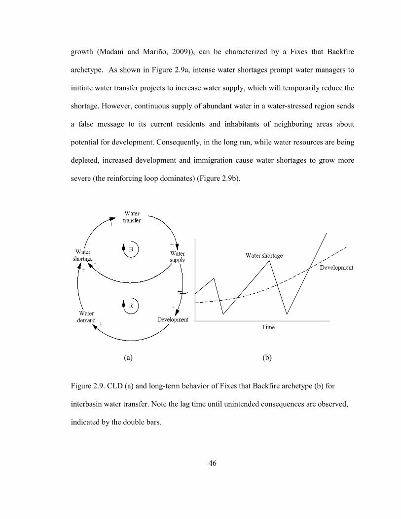
46
growth (Madani and Mariño, 2009)), can be characterized by a Fixes that Backfire
archetype. As shown in Figure 2.9a, intense water shortages prompt water managers to
initiate water transfer projects to increase water supply, which will temporarily reduce the
shortage. However, continuous supply of abundant water in a water-stressed region sends
a false message to its current residents and inhabitants of neighboring areas about
potential for development. Consequently, in the long run, while water resources are being
depleted, increased development and immigration cause water shortages to grow more
severe (the reinforcing loop dominates) (Figure 2.9b).
(a) (b)
Figure 2.9. CLD (a) and long-term behavior of Fixes that Backfire archetype (b) for
interbasin water transfer. Note the lag time until unintended consequences are observed,
indicated by the double bars.

47
2.4.5.3. Success to the successful
The Success to the Successful archetype states that good performance will earn an
entity more resources, making it possible for the entity to generate even better results and
gain still more resources. Dominance of this archetype in a natural setting where
resources are limited can deprive the weaker competitors of the resources they need to
improve their condition and become more competitive. Consequently, the successful
entity continuously grows while other entities gradually decline and possibly collapse.
This archetype can ultimately result in considerable inequity and imbalance among
entities (e.g., water resources stakeholders), threatening the system’s sustainability.
Supply-oriented water resources management in a large metropolitan area can be
explained using the Success to the Successful archetype, illustrated in Figure 2.10a.
Water scarcity in less-populated neighboring areas is secondary to the needs of a water-
stressed megacity (Bagheri and Hjorth, 2007). As the megacity’s share of water resources
increases, so does potential for development, which in turn adds to the power of the
megacity to gain more water resources. Simultaneously, the neighboring towns’ share of
water resources decreases, hindering their development and ability to gain necessary
resources (Figure 2.10b). Another real example of a water resources problem based on
the Success to the Successful archetype is floodplain development in California, which
results in a continuous profit to the local developers (success) and continuous increase in
risk of economic loss to the state of California as a result of development behind
unreliable levees (Madani et al., 2007).
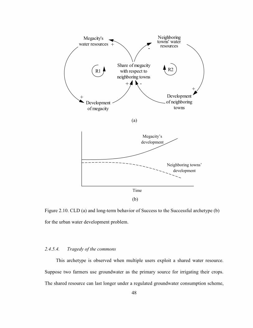
48
(a) (b)
Figure 2.10. CLD (a) and long-term behavior of Success to the Successful archetype (b)
for the urban water development problem.
2.4.5.4. Tragedy of the commons
This archetype is observed when multiple users exploit a shared water resource.
Suppose two farmers use groundwater as the primary source for irrigating their crops.
The shared resource can last longer under a regulated groundwater consumption scheme,
Megacity'swater resources
Developmentof megacity
Share of megacitywith respect to
neighboring towns
Neighboringtowns' water
resources
Developmentof neighboring
towns
+
+
+-
+-
R1 R2
Time
Neighboring towns’ development
Megacity’s development
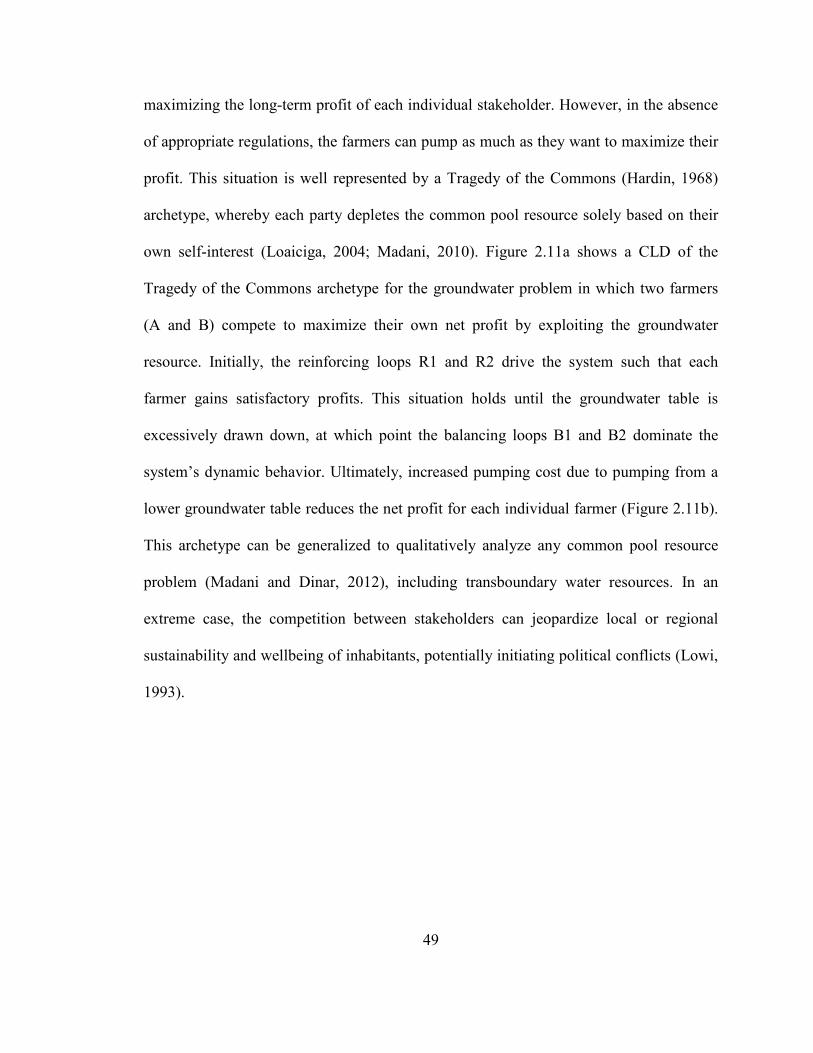
49
maximizing the long-term profit of each individual stakeholder. However, in the absence
of appropriate regulations, the farmers can pump as much as they want to maximize their
profit. This situation is well represented by a Tragedy of the Commons (Hardin, 1968)
archetype, whereby each party depletes the common pool resource solely based on their
own self-interest (Loaiciga, 2004; Madani, 2010). Figure 2.11a shows a CLD of the
Tragedy of the Commons archetype for the groundwater problem in which two farmers
(A and B) compete to maximize their own net profit by exploiting the groundwater
resource. Initially, the reinforcing loops R1 and R2 drive the system such that each
farmer gains satisfactory profits. This situation holds until the groundwater table is
excessively drawn down, at which point the balancing loops B1 and B2 dominate the
system’s dynamic behavior. Ultimately, increased pumping cost due to pumping from a
lower groundwater table reduces the net profit for each individual farmer (Figure 2.11b).
This archetype can be generalized to qualitatively analyze any common pool resource
problem (Madani and Dinar, 2012), including transboundary water resources. In an
extreme case, the competition between stakeholders can jeopardize local or regional
sustainability and wellbeing of inhabitants, potentially initiating political conflicts (Lowi,
1993).
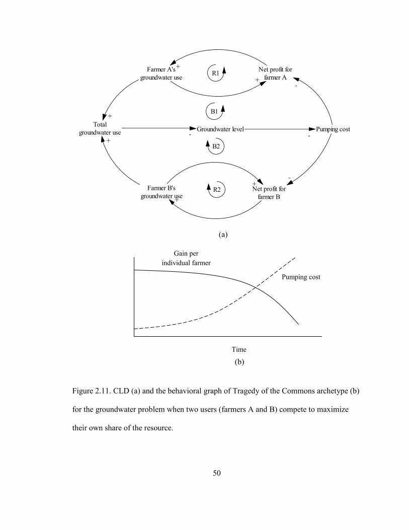
50
(a)
(b)
Figure 2.11. CLD (a) and the behavioral graph of Tragedy of the Commons archetype (b)
for the groundwater problem when two users (farmers A and B) compete to maximize
their own share of the resource.
Net profit forfarmer A
Farmer A'sgroundwater use
Totalgroundwater use
Farmer B'sgroundwater use
Net profit forfarmer B
Groundwater level
+
+
+
+
+
+
R1
R2
B1
B2
Pumping cost-
-
-
-
Time
Gain per individual farmer
Pumping cost
51
2.5. Discussion
2.5.1. Qualitative versus quantitative modeling
Qualitative system dynamics modeling can be used at different levels for different
purposes (Richmond, 1994). Randers (1980) believes that “most human knowledge takes
a descriptive non-quantitative form”, and thus analysts should not restrict themselves to
numerical data, which is a small fraction of knowledge fit for statistical analysis.
However, developing qualitative models may not be enough for complete analysis of the
problem. Proponents of quantitative modeling argue that numerical simulation nearly
always adds value, even in the face of significant uncertainties about data and important
qualitative information used in simulations (Forrester, 1975; Homer and Oliva, 2001;
Dhawan et al., 2011). It is necessary to recognize the pitfall of oversimplifying a problem
and neglecting the value of conducting detailed simulations, which may reveal complex
system behaviors that could not be understood through simple diagramming (Homer and
Oliva, 2001; Forrester, 2007). However, to accomplish a successful system dynamics
application, extensive computer simulations should be performed only after a clear
picture of the integrated water resources system has been established through reasonably
simplified conceptual models. Contrary to conventional modeling which may fail to
capture the big picture of the problem with important feedback loops, a thorough system
dynamics study can provide reliable qualitative and quantitative bases for policy
selection. In this way, instead of investing resources prematurely, analysts can prioritize
what to study in more detail to ensure an in-depth understanding of the problem is
obtained.
52
System dynamics’ qualitative modeling tools, and the insights that they provide,
make this approach accessible to a wide range of decision makers and stakeholders. The
tools for visually exploring systems are a major distinguishing factor between this
approach and traditional simulation methods. These qualitative analysis tools help
generate a constructive medium for understanding a system’s structure using an iterative
approach best implemented through interaction with people who are familiar with the
system at different levels (Randers, 1980). Therefore, attempts to reveal the main drivers
of the problem using CLDs, SFDs, and archetypes are necessary. However, analysts
should be aware of the general concerns about using qualitative modeling tools. In
particular, problems might be encountered when translating CLDs into SFDs. Richardson
(1986) argues that traditional definitions of the polarities of causal links and feedback
loops are inadequate. In order to address this inadequacy he suggests that CLDs should
account for the accumulating nature of the Flow-to-Stock links. As an alternative way for
dealing with this problem, modelers can use CLDs along with reasonably representative
SFDs to ensure qualitative insights are properly communicated.
System archetypes provide generic CLDs that reveal qualitative information about
the underlying structure of the system, enabling water managers to detect current
problematic trends and anticipate future problems. Thus, system archetypes are not meant
to address any specific problem, but instead are applicable to classes of problems that
share one or more modes of dynamic behavior. For various classes of problems, generic
solution archetypes have been reported in the literature (Wolstenholme, 2004). As such,
system archetypes can be used along with other system dynamics tools such as SFDs to
generate a broad, holistic understanding of the system’s state and its long-term behavioral
53
pattern. Essentially, once analysts reach a consensus regarding the system archetype that
governs their particular system of interest, they can obtain valuable insights into solution
strategies, which can be further analyzed and tested using detailed simulations
(Wolstenholme, 2003). This is a unique characteristic of system dynamics that facilitates
conceptual or high-level strategic water resources modeling.
System dynamics models should have comprehensive, and yet simple structures,
particularly when presented to non-technical audiences (Stave, 2003). In this context,
simplicity is not equivalent to misrepresentation of the system’s structure. Rather, it is
more consistent with Albert Einstein’s maxim that “a good explanation is one that is as
simple as possible, but not simpler.” Often, it is also important for system dynamics
water resources models to have transparent structures that facilitate sensitivity analysis,
which is critical for adaptive water resources management and scenario-based policy
screening (Simonovic and Fahmy, 1999). If too much detail is included in the CLD, the
structure of the system dynamics model may become overly difficult to understand for
people who have not been involved in the model development. In addition to increased
data requirements for complex, integrated models, to be able to provide meaningful
interpretation of behavioral trends modelers must develop appropriate methods and
protocols for quantifying socio-political subsystems--a task which remains a formidable
challenge (Hellström et al., 2000; Luna-Reyes and Andersen, 2003). Furthermore,
regardless of the scope of the problem, modelers need to apply appropriate aggregation
and hierarchical decomposition principles to accomplish the modeling task, with the level
of aggregation and decomposition varying according to the scale of problem, modeling
objectives, and desired model sophistication.
54
2.5.2. Validation of system dynamics models
Model “verification” or “validation”, i.e., testing of the model using an independent
data set, is often problematic due to limited data and, in some cases, a lack of appropriate
methods for quantifying particular (e.g., socio-political) subsystems. Sterman (2000), in
fact, argues that no model can ever be verified or validated, for models are simplified
representations of real processes and are thus different from reality in infinitely many
ways. Nevertheless, in order for models to be useful as decision support tools for water
resources planning and management, it is necessary to verify the model structure to
ensure that mathematical equations and interrelationships between subsystems follow
logical explanations and are not spurious or erroneous. Unlike purely data-driven black-
box models, generating an “accurate” output behavior is not sufficient for validation of
causal-descriptive white-box system dynamics models, which in addition to reproducing
the system behavior, should explain how the behavior is generated (Barlas 1996). Thus,
as Barlas (1996) explains, in the context of system dynamics, model validation is a semi-
formal process consisting of a balanced mix of both quantitative tests and qualitative
behavioral criteria targeting the system’s internal structure. In participatory system
dynamics modeling, validation can be done throughout model development by a range of
experts and stakeholders, which may be much more reliable than an external review of
the model at the end of the process. The verification phase of system dynamics models
developed for water resources problems has not always been discussed in detail, but
modelers have reported a variety of verification methods, including behavior replication,
sensitivity analysis, dimensional consistency, and structure assessment (Ahmad and
55
Simonovic, 2000; Stave, 2003; Tangirala et al., 2003). Table 2.6 summarizes these
methods of verification of water resources system dynamics models.
2.5.3. Strengths and limitations of system dynamics modeling
To summarize, Table 2.7 lists the major benefits and potential pitfalls of holistic
water resources system dynamics models, including problems which might arise due to
inappropriate application of the method without proper regard for its philosophy. Caution
should be used when interpreting system dynamics models, for it is easy to formulate
erroneous dynamic hypotheses due to inadequate information about a complex system, or
due to lack of expertise. Biased simulation results may stem from faulty CLDs and SFDs.
This caveat is particularly important when creating integrated models to simulate
feedback relationships among socio-economic, political, natural, and technological
subsystems. Tradeoffs among accuracy, breadth, and time must be considered in any
modeling study. Nevertheless, although quantification of socio-economic and political
components of water resources systems is challenging, and sometimes even speculative
(Madani and Mariño, 2009), system dynamics modeling helps to prioritize information
gathering and holistically investigate interactions and potential impacts of different
drivers of the problem.
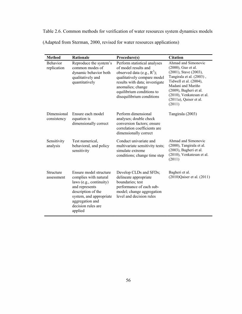
56
Table 2.6. Common methods for verification of water resources system dynamics models
(Adapted from Sterman, 2000, revised for water resources applications)
Method Rationale Procedure(s) Citation Behavior replication
Reproduce the system’s common modes of dynamic behavior both qualitatively and quantitatively
Perform statistical analyses of model results and observed data (e.g., R2); qualitatively compare model results with data; investigate anomalies; change equilibrium conditions to disequilibrium conditions
Ahmad and Simonovic (2000), Guo et al. (2001), Stave (2003), Tangirala et al. (2003) , Tidwell et al. (2004), Madani and Mariño (2009), Bagheri et al. (2010), Venkatesan et al. (2011a), Qaiser et al. (2011)
Dimensional consistency
Ensure each model equation is dimensionally correct
Perform dimensional analyses; double check conversion factors; ensure correlation coefficients are dimensionally correct
Tangirala (2003)
Sensitivity analysis
Test numerical, behavioral, and policy sensitivity
Conduct univariate and multivariate sensitivity tests; simulate extreme conditions; change time step
Ahmad and Simonovic (2000), Tangirala et al. (2003), Bagheri et al. (2010), Venkatesan et al. (2011)
Structure assessment
Ensure model structure complies with natural laws (e.g., continuity) and represents description of the system, and appropriate aggregation and decision rules are applied
Develop CLDs and SFDs; delineate appropriate boundaries; test performance of each sub-model; change aggregation level and decision rules
Bagheri et al. (2010)Qaiser et al. (2011)
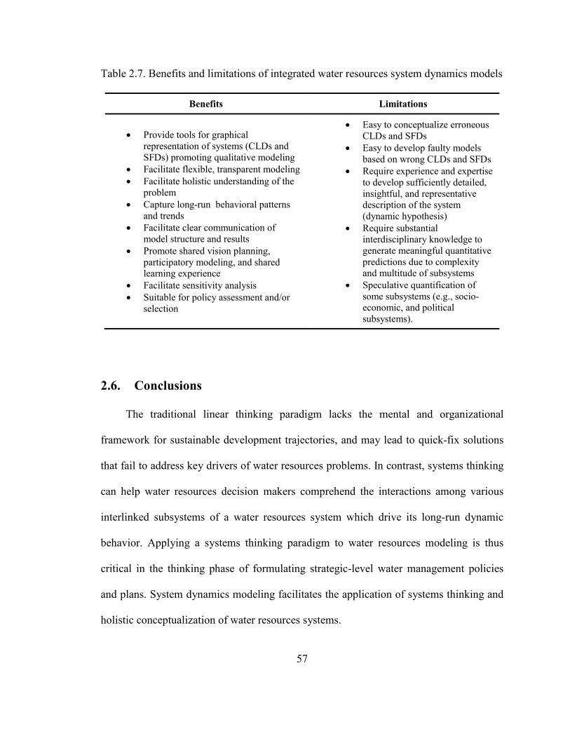
57
Table 2.7. Benefits and limitations of integrated water resources system dynamics models
Benefits Limitations
• Provide tools for graphical representation of systems (CLDs and SFDs) promoting qualitative modeling
• Facilitate flexible, transparent modeling • Facilitate holistic understanding of the
problem • Capture long-run behavioral patterns
and trends • Facilitate clear communication of
model structure and results • Promote shared vision planning,
participatory modeling, and shared learning experience
• Facilitate sensitivity analysis • Suitable for policy assessment and/or
selection
• Easy to conceptualize erroneous CLDs and SFDs
• Easy to develop faulty models based on wrong CLDs and SFDs
• Require experience and expertise to develop sufficiently detailed, insightful, and representative description of the system (dynamic hypothesis)
• Require substantial interdisciplinary knowledge to generate meaningful quantitative predictions due to complexity and multitude of subsystems
• Speculative quantification of some subsystems (e.g., socio-economic, and political subsystems).
2.6. Conclusions
The traditional linear thinking paradigm lacks the mental and organizational
framework for sustainable development trajectories, and may lead to quick-fix solutions
that fail to address key drivers of water resources problems. In contrast, systems thinking
can help water resources decision makers comprehend the interactions among various
interlinked subsystems of a water resources system which drive its long-run dynamic
behavior. Applying a systems thinking paradigm to water resources modeling is thus
critical in the thinking phase of formulating strategic-level water management policies
and plans. System dynamics modeling facilitates the application of systems thinking and
holistic conceptualization of water resources systems.
58
In recent decades, while system dynamics has been widely used by water resources
scholars as a tool for quantitative water resources modeling, it has not typically been
utilized to its full capacity for scrutinizing the system’s structure to provide insights into
potential reasons behind problematic behavioral trends. At the strategic level, emphasis
should be placed on trend identification and pattern recognition rather than exact
quantitative predictions of dynamic variables. Although the quantitative modeling phase
using extensive computer simulations is still very important and needed for policy
screening, especially when characterizing complex systems, qualitative system dynamics
models can improve understanding of general trends and the root causes of problems, and
thus promote sustainable water resources decision making.
In this chapter, tangible water resources examples were presented to illustrate the
fundamentals of system dynamics, emphasizing that developing CLDs and SFDs is
necessary for identifying causal relationships forming feedback loops within water
resources systems. Furthermore, water managers should use the knowledge of reference
modes and system archetypes (e.g., Limits to Growth, Fixes that Backfire, Success to the
Successful, and Tragedy of the Commons) to gain insights into sustainable solution
strategies by recognizing common patterns of dynamic behavior. Compared to other
modeling approaches, perhaps the most significant advantage of system dynamics is that
when systems are not too complicated, the qualitative modeling tools can help describe
the behavior of many variables, even before quantitative (numerical) modeling begins.
This characteristic facilitates conceptual or high-level strategic water resources modeling
using multi-disciplinary, multi-sectoral, and participatory approaches critical to
sustainable water resources planning and management.
59
2.7. References
Ahmad, S., Simonovic, S.P. (2000). System dynamics modeling of reservoir operations
for flood management. Journal of Computing in Civil Engineering 14(3), 190–
198.
Ahmad, S., Simonovic, S.P. (2004). Spatial system dynamics: a new approach for
simulation of water resources systems. Journal of Computing in Civil Engineering
18(4), 331-340.
Ahmad, S., Prashar, D. (2010). Evaluating municipal water conservation policies using a
dynamic simulation model. Water Resources Management 24(13), 3371-3395.
Bagheri, A., Hjorth, P. (2007). A framework for process indicators to monitor for
sustainable development: practice to an urban water system. Environmental
Development and Sustainability 9(2), 143–161.
Bagheri, A., Darijani, M., Asgary, A., Morid, S. (2010). Crisis in urban water systems
during the reconstruction period: a system dynamics analysis of alternative
policies after the 2003 earthquake in Bam-Iran. Water Resources Management
24(11), 2567-2596.
Barlas, Y. (1996). Formal aspects of model validity and validation in system dynamics.
System Dynamics Review 12 (3), 183-210.
Cai, X., Wang, D. (2006). Calibrating holistic water resources-economic models. Journal
of Water Resources Planning and Management 132(6), 414–423.
60
Coyle, G. (2000). Qualitative and quantitative modelling in system dynamics: Some
research questions. System Dynamics Review 16(3), 225–244.
Creighton, J.L., Langsdale, S. (2009). Analysis of process issues in shared vision
planning cases, IWR Report 09-R-05, Institute for Water Resources, U.S. Army
Corps of Engineers, Alexandria, Virginia.
Davies, E.G.R., Simonovic, S.P. (2011). Global water resources modeling with an
integrated model of the social–economic–environmental system. Advances in
Water Resources 34, 684-700.
Dhawan, R., O'Connor, M., Borman, M. (2011). The effect of qualitative and quantitative
system dynamics training: an experimental investigation. System Dynamics
Review (2011).doi: 10.1002/sdr.455
Erickson, J.D., Gowdy, J.M. (2000). Resource use, institutions and sustainability: a tale
of two Pacific island cultures. Land Economics 76(3), 345– 354.
Ford, A. (1996). Testing the Snake River Explorer. System Dynamics Review 12(4), 305-
329.
Ford, A. (1999). Modeling the environment. Island Press, Washington.
Forrester, J. (1961). Industrial dynamics. MIT Press, Cambridge.
Forrester, J. (1975). Industrial dynamics—a response to Ansoff and Slevin. In: Collected
Papers of Jay W. Forrester. Wright-Allen Press, Cambridge, Massachusetts, pp
151–165.
Forrester, J. (1969). Urban dynamics. MIT Press, Cambridge.
Forrester, J. (2007). System dynamics—the next fifty years. System Dynamics Review 23,
359-370.
61
Gastélum, J.R., Valdés, J.B., Stewart, S. (2009). A decision support system to improve
water resources management in the Conchos Basin. Water Resources
Management 23(8), 1519–1548.
Guo, H.C., Liu, L., Huang, G.H., Fuller, G.A., Zou, R., Yin, Y.Y. (2001). A system
dynamics approach for regional environmental planning and management: a study
for the Lake Erhai Basin. Environmental Management 61(1), 93–111.
Hardin, G. (1968). The tragedy of the commons. Science 162, 1243-1248.
Hellström, D., Jeppsson, U., Kärrman, E. (2000). A framework for systems analysis of
sustainable urban water management. Environmental Impact Assessment Review
20(3), 311–321.
High Performance Systems (1992) Stella II: an introduction to systems thinking. High
Performance Systems, Inc., Hanover, New Hampshire.
Hjorth, P., Bagheri, A. (2006). Navigating towards sustainable development: a system
dynamics approach. Futures 38(1), 74–92.
Homer, J., Oliva, R. (2001). Maps and models in system dynamics: a response to Coyle.
System Dynamics Review 17(4), 347-356.
Langsdale, S., Beall, A., Carmichael, J., Cohen, S., Forster, C. (2007). An exploration of
water resources futures under climate change using system dynamics modeling.
Integrated Assessment 7 (1), 51-79.
Langsdale, S., Beall, A., Carmichael, J., Cohen, S., Forster, C., Neale, T. (2009).
Exploring the implications of climate change on water resources through
participatory modeling: case study of the Okanagan Basin, British Columbia.
Journal of Water Resources Planning and Management 135(5), 373–381.
62
Leal Neto, A.C., Legey, L.F.L., Gonzalez-Araya, M.C., Jablonski, S. (2006). A system
dynamics model for the environmental management of the Sepetiba Bay
watershed, Brazil. Environmental Management 38(5), 879–888.
Leaver, J.D., Unsworth, C.P. (2006). System dynamics modeling of spring behaviour in
the Orakeikorako geothermal field, New Zealand. Geothermics 36(2), 101-114.
Loaiciga, H.A. (2004). Analytic game - theoretic approach to ground-water extraction.
Journal of Hydrology 297, 22-33.
Lowi, M, (1993). Water and power – the politics of a scarce resource in the Jordan River
Basin. Cambridge University Press, Cambridge.
Luna-Reyes, L.F., Andersen, D.L. (2003). Collecting and analyzing qualitative data for
system dynamics: methods and models. System Dynamics Review 19(4), 271-296.
Lund, J.R., Palmer, R.N. (1997). Water resource system modeling for conflict resolution.
Water Resources Update, Universities Council on Water Resources 108, 70–82.
Madani, K. (2010) Game theory and water resources. Journal of Hydrology 381 (3-4),
225-238.
Madani, K., Dinar, A. (2012). Non-cooperative institutions for sustainable common pool
resource management: application to groundwater. Ecological Economics 74, 34-
45.
Madani, K., Mariño, M.A. (2009). System dynamics analysis for managing Iran’s
Zayandeh-Rud river basin. Water Resources Management 23 (11), 2163-2187.
Madani, K., Rowan, D., Lund, J.R. (2007). The next step in Central Valley flood
management: connecting costs and benefits. In: Proceedings of the University
Council on Water Resources Annual Conference, Boise, Idaho.
63
McMahon, G.F., Farmer, M.C. (2004). Reallocation of federal multipurpose reservoirs:
principles, policy, and practice. Journal of Water Resources Planning and
Management 130(3), 187-197.
Meadows, D.H., Meadows, D.L., Randers, J., Behrens, W.W. (1972). The limits to
growth. Universe Books, New York.
Mirchi, A., Watkins, D.W. Jr, Madani, K. (2010) Modeling for watershed planning,
management and decision making. In: Vaughn JC (ed) Watersheds management,
restoration and environmental impact. Nova Science Publishers, Hauppauge, New
York.
Powersim Corporation (1996). Powersim 2.5 reference manual. Powersim Corporation
Inc., Herndon, Virginia.
Qaiser, K., Ahmad, S., Johnson, W., Batista, J. (2011). Evaluating the impact of water
conservation on fate of outdoor water use: a study in an arid region. Journal of
Environmental Management 92(8), 2061-2068.
Randers, J. (1980). Guidelines for model conceptualization. In: Randers J (ed) Elements
of the system dynamics method. MIT Press: Cambridge, Massachusetts, pp 117–
139.
Richardson, G.P. (1986). Problems with causal-loop diagrams. System Dynamics Review
2, 158-170.
Richmond, B. (1993). Systems thinking: critical thinking skills for the 1990ies and
beyond. System Dynamics Review 9(2), 113 – 133.
Richmond, B. (1994). Systems thinking/system dynamics: let’s just get on with it. System
Dynamics Review 10(2/3), 135-57.
64
Saeed, K. (1998). Defining a problem or constructing a reference mode. In: Proceedings
of the 16th International Conference of the System Dynamics Society Quebec '98,
Quebec City, Canada.
Sehlke, G., Jacobson, J. (2005). System dynamics modeling of transboundary systems:
the Bear River Basin model. Ground Water 43(5), 722–730.
Senge, P. (1990). The Fifth Discipline: the art & practice of the learning organization.
Doubleday/Currency, New York.
Simonovic, SP. (2009). Managing water resources: methods and tools for a systems
approach. UNESCO, Paris and Earthscan James & James, London.
Simonovic, S.P., Ahmad, S. (2005) Computer-based model for flood evacuation
emergency planning. Natural Hazards 34(1), 25-51.
Simonovic, S.P., Fahmy, H. (1999). A new modeling approach for water resources policy
analysis. Water Resources Research 35(1), 295–304.
Simonovic, S.P., Li, L. (2003). Methodology for assessment of climate change impacts
on large-scale flood protection system. Journal of Water Resources Planning and
Management 129(5), 361–371.
Simonovic, S.P., Rajasekaram, V. (2004). Integrated analyses of Canada’s water
resources: a system dynamics approach. Canadian Water Resources Journal
29(4), 223–250.
Stave, K.A. (2003). A system dynamics model to facilitate public understanding of water
management options in Las Vegas, Nevada. Environmental Management 67(4),
303–313.
65
Sterman, J.D. (2000). Business dynamics, systems thinking and modeling for a complex
world. McGraw-Hill, Boston.
Stewart, S., Valdés, J., Gastélum, J., Brookshire, D., Aparicio, J., Hidalgo, J., Velazco, I.
(2004). A decision support system for demand management in the Rio Conchos
Basin, México. In: Proceedings of hydrology: science & practice for the 21st
Century. British Hydrological Society II, pp 487–494.
Tangirala, A.K., Teegavarapu, R.S.V., Ormsbee, L. (2003). Modeling adaptive water
quality management strategies using system dynamics simulation. Environmental
Informatics Archives 1, 245-253.
Tidwell, V.C., Passell, H.D., Conrad, S.H., Thomas, R.P. (2004). System dynamics
modeling for community-based water planning: application to the Middle Rio
Grande. Aquatic Sciences 66, 357–372.
Venkatesan, A.K., Ahmad, S., Johnson, W., Batista, J.R. (2011a). Salinity reduction and
energy conservation in direct and indirect potable water reuse. Desalination 272
(1-3),120-127.
Venkatesan, A.K., Ahmad, S., Johnson, W., Batista, J.R. (2011b). System dynamics
model to forecast salinity load to the Colorado River due to urbanization within
the Las Vegas Valley. Science of the Total Environment 409, 2616-2625.
Ventana Systems (1996) Vensim user’s guide. Ventana Systems Inc., Belmont,
Massachusetts.
Vezjak, M., Savsek, T., Stuhler, E.A. (1998). System dynamics of eutrophication
processes in lakes. European Journal of Operational Research 109(2), 442-451.
66
Watkins, D.W. Jr, Moser, D.A. (2006). Economic-based optimization of Panama Canal
system operations. Journal of Water Resources Planning and Management
132(6), 426-438.
Werick, W.J., Whipple, W. (1994). Managing Water for Drought, IWR Report 94-NDS-
8, Institute for Water Resources, U.S. Army Corps of Engineers, Alexandria,
Virginia.
Winz, I., Brierley, G., Trowsdale, S. (2009). The use of system dynamics simulation in
water resource management. Water Resources Management 23(7), 1301–1323.
Wolstenholme, E.F. (1999). Qualitative vs. quantitative modelling: the evolving balance.
In: Coyle RG, Morecroft JDW (eds) Special issue: system dynamics for policy,
strategy and management education. Journal of the Operational Research Society
50(4), 354-361.
Wolstenholme, E.F. (2003). Towards the definition and use of a core set of archetypal
structures in system dynamics. System Dynamics Review 19(1), 7–26.
Wolstenholme, E.F. (2004). Using generic system archetypes to support thinking and
modelling. System Dynamics Review 20, 341–356.
Wolstenholme, E.F., Coyle, R.G. (1983). The development of system dynamics as a
methodology for system description and qualitative analysis. Journal of the
Operational Research Society 34(7), 569–581.
Xu, Z.X., Takeuchi, K., Ishidaira, H., Qhang, X.W. (2002). Sustainability analysis for
Yellow River water resources using the system dynamics approach. Water
Resources Management 16(3), 239–261.
67
Chapter 3 - A systems approach to holistic TMDL policy: Case of Lake Allegan, Michigan3
3.1. Abstract
Systems thinking can provide insights for developing effective plans to protect
environmental integrity of natural systems impacted by human activities. In this study, a
system dynamics archetype governing Lake Allegan’s eutrophication problem is
hypothesized to explain the system’s problematic behavior and identify policy leverage
points for mitigation. To operationalize the systems thinking concepts, an integrated
system dynamics model is developed to simulate the interaction between key socio-
economic subsystems and natural processes driving eutrophication. The model is applied
to holistically characterize the lake’s recovery from its hypereutrophic state and assess a
number of proposed TMDL reduction policies, including phosphorus load reductions
from point sources and non-point sources. It is shown that, for a TMDL plan to be
effective, it should be considered a component of a continuous sustainability process,
which considers the functionality of dynamic feedback relationships between socio-
economic growth, land use change, and environmental conditions.
3 This chapter is a reprint of the article: Mirchi, A., Watkins, D.W. Jr., 2012. A systems approach to
holistic TMDL policy: Case of Lake Allegan, Michigan. Journal of Water Resources Planning and
Management, doi: 10.1061/(ASCE)WR.1943-5452.0000292. Reprinted with permission from the American
Society of Civil Engineers (ASCE).
68
3.2. Introduction
Extensive socio-economic development without proper regard for environmental
integrity and ecosystem resilience can result in unsustainable development (Bishop,
1993; Arrow et al., 1995). For instance, nutrient enrichment of water bodies causing loss
of biodiversity may be symptomatic of a human-induced environmental degradation
known as cultural eutrophication (Cooke et al., 1993; Effler et al., 2002). A fundamental
premise for this study is that population growth, affluence, and technology are three
critical factors that drive anthropogenic environmental change (Ehrlich and Holdren,
1971). Important feedback relationships exist between socio-economic growth and
environmental damage, although environmental degradation may not be severe enough to
stop the growth process within the typical planning timeframes (Arrow et al., 1995).
Ehrlich and Holdren's theorem provides a contextual foundation for understanding the
potential impacts of the linkage between socio-economic dynamics and lake phosphorus
(P) concentration on the success or failure of human intervention to maintain and/or
improve environmental integrity.
The Federal Water Pollution Control Act Amendment of 1972, commonly known
as the Clean Water Act (CWA), introduced the concept of Total Maximum Daily Load
(TMDL) to guide water quality management in the US (FWPCA, 1972). TMDL is a
written plan prescribing the maximum amount of pollutant loads that a water body can
receive without violating predefined water quality standards. The CWA amendment of
2002 requires each state to identify the main pollutant(s) impacting the impaired water
bodies, and to meet necessary water quality standards using TMDLs, i.e., quantifying
allowable levels of load allocation and waste-load allocation (FWPCA, 2002). In this
69
context, load allocation refers to pollutant loads from non-point sources (NPS) along with
natural background inputs, whereas waste-load allocation is the allowable pollutant load
from point sources (PS). Furthermore, a margin of safety is considered to compensate for
lack of knowledge as to relationship between pollutant inputs and water quality
(FWPCA, 2002). Comprehensive TMDL plans are very challenging due to economic,
legal, and political aspects of TMDL implementation. Nevertheless, inclusion of both PSs
and NPSs of pollution rather than only applying restrictions on end-of-pipe discharges,
partly addresses the concern that TMDL plans overemphasize the contribution of PSs
without adequately accounting for nutrient loads from NPSs (Boyd, 2000).
TMDL plans have been widely implemented in the US (e.g., Benham et al., 2008).
However, many TMDL studies do not address the dynamic socio-economic setting of the
problem, as this has neither been mandated by law nor adequately addressed in the
TMDL literature. While many TMDL studies have identified NPS pollution to be a major
driver of eutrophication, land use change driven by socio-economic development is often
not accounted for when proposing nutrient reduction levels to reach the prescribed water
quality targets. This shortcoming is particularly critical because the NPS component of
TMDL plans is typically founded on average nutrient loads that are calculated for
different land use categories by conducting limited monitoring programs and/or using
literature values. Although physical aspects of water quality problems have been the
subject of extensive research, including modeling and quantitative analyses addressing
spatiotemporal variability and uncertainty (e.g., Doerr et al., 1996; Haven and Schelske,
2001; Vondracek et al., 2003; Shirmohammadi et al., 2006; Canale et al., 2010), little
70
attention has been paid to the interplay of socio-economic and land use dynamics and
their implications for water quality problems (Vergura and Jones, 2000).
Adopting a systems thinking approach and applying system dynamics (SD)
modeling (Forrester, 1961 and 1969; Senge, 1990; Ford, 1999; Sterman, 2000;
Simonovic, 2009) can facilitate holistic understanding of TMDL problems, and may thus
guide the formulation of long-term TMDL plans. TMDL studies are inherently
multidisciplinary as they should characterize a host of physical, ecological, and
biogeochemical processes. Socio-economic characteristics of the study area add yet
another piece to the puzzle. SD provides useful qualitative and quantitative tools for
characterizing different feedback loops that govern water resources systems (Simonovic
and Fahmy, 1999; Hjorth and Bagheri, 2006; Madani and Mariño, 2009). Winz et al.
(2009) reviewed water resources SD literature to illustrate its use in integrated water
resources management. Researchers have used SD for simulating biophysical processes
to develop decision support tools for water quality management (Vezjak et al., 1998).
Furthermore, SD has been used in integrated analysis of water quality problems and
environmental deterioration by linking regional-scale physical and socio-economic
subsystems to water quality models (Guo et al., 2001; Leal Neto et al., 2006).
Failing to recognize and appropriately account for the feedbacks between socio-
economic and natural sub-systems may lead to inadequate nutrient reduction plans in the
long-term. Understanding causal structures driving the system’s long-run behavior, and
using this information to formulate integrated TMDL plans provides opportunities for
holistic policy making to direct water quality management (Boyd, 2000). Hence, there is
a need for a framework to conceptualize the eutrophication problem, and quantify the
71
processes to help describe the system’s long-run behavior to decision makers and
stakeholders, increasing support for the proposed nutrient reduction measures. The
eutrophication problem of Lake Allegan, Michigan, is used as a case study to
demonstrate the potential long-term role of socio-economic factors in nutrient loading of
water bodies. The problem is explained using the “Growth and Underinvestment” system
archetype (Senge, 1990), illustrating the need for making sufficient investment in
maintaining environmental integrity to allow for sustained economic growth.
3.3. Lake Allegan’s Eutrophication Problem
Lake Allegan is a 647.5-hectare impoundment formed by the Calkins Dam on the
Kalamazoo River in Southwestern Michigan, USA (Figure 3.1). Located at the outlet of a
401,500-hectare drainage area within the Kalamazoo River watershed, the lake has a
volume of approximately 21.22 million m3 with a mean and maximum depth of about
3.35m and 6.1m, respectively, and a short mean hydraulic retention time of seven days
(US EPA, 1975). The impoundment has altered the Kalamazoo River sediment transport
pattern and water quality by trapping most sediment and associated pollutants (MDNR,
1987). Lake Allegan receives water from the Kalamazoo River with a mean flow of about
35.1 m3/s, and from Dumont Creek and other minor tributaries, and direct drainage from
surrounding areas, collectively increasing the lake’s mean total inflow to about 36 m3/s,
which eventually discharges into Lake Michigan (US EPA, 1975). In 1978, agriculture
was the dominant land use type covering about 50% of the lake’s watershed area,
followed by 34% forest/open land. The rest of the watershed land use was characterized
by 8% urban and built-up and 7% water/wetland.
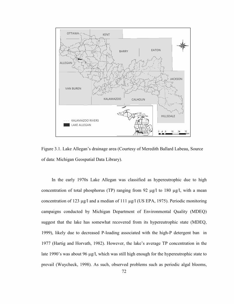
72
Figure 3.1. Lake Allegan’s drainage area (Courtesy of Meredith Ballard Labeau, Source
of data: Michigan Geospatial Data Library).
In the early 1970s Lake Allegan was classified as hypereutrophic due to high
concentration of total phosphorus (TP) ranging from 92 µg/l to 180 µg/l, with a mean
concentration of 123 µg/l and a median of 111 µg/l (US EPA, 1975). Periodic monitoring
campaigns conducted by Michigan Department of Environmental Quality (MDEQ)
suggest that the lake has somewhat recovered from its hypereutrophic state (MDEQ,
1999), likely due to decreased P-loading associated with the high-P detergent ban in
1977 (Hartig and Horvath, 1982). However, the lake’s average TP concentration in the
late 1990’s was about 96 µg/l, which was still high enough for the hypereutrophic state to
prevail (Wuycheck, 1998). As such, observed problems such as periodic algal blooms,
73
excessive turbidity, low dissolved oxygen levels, and imbalance in fish populations are
largely attributable to high TP concentration (Wuycheck, 1998).
Since 1998 P reduction plans have been implemented in the Lake Allegan
watershed to reduce the growing season (April-September) TP concentration of the lake
to 60 µg/l by 2015 (Heaton, 2001; KRLATIC, 2002). Kieser and Associates (2001)
conducted a spatiotemporal analysis of the water quality throughout the Lake Allegan
drainage area and recommended that PS loadings to the lake be cut back by 23% and that
NPS loadings be reduced by 50% (Kieser and Associates, 2001). Table 3.1 presents the
breakdown of the proposed TMDL components for Lake Allegan during growing season
(April-September). While PS discharges have effectively complied with the prescribed
waste-load allocation throughout the decade following the implementation of Lake
Allegan’s TMDL plan, the lake’s recovery appears to be taking longer than anticipated.
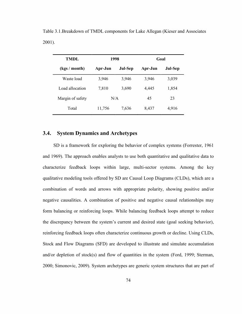
74
Table 3.1.Breakdown of TMDL components for Lake Allegan (Kieser and Associates
2001).
TMDL
1998 Goal
(kgs / month) Apr-Jun Jul-Sep Apr-Jun Jul-Sep
Waste load
3,946 3,946 3,946 3,039
Load allocation 7,810 3,690 4,445 1,854
Margin of safety N/A 45 23
Total 11,756 7,636 8,437 4,916
3.4. System Dynamics and Archetypes
SD is a framework for exploring the behavior of complex systems (Forrester, 1961
and 1969). The approach enables analysts to use both quantitative and qualitative data to
characterize feedback loops within large, multi-sector systems. Among the key
qualitative modeling tools offered by SD are Causal Loop Diagrams (CLDs), which are a
combination of words and arrows with appropriate polarity, showing positive and/or
negative causalities. A combination of positive and negative causal relationships may
form balancing or reinforcing loops. While balancing feedback loops attempt to reduce
the discrepancy between the system’s current and desired state (goal seeking behavior),
reinforcing feedback loops often characterize continuous growth or decline. Using CLDs,
Stock and Flow Diagrams (SFD) are developed to illustrate and simulate accumulation
and/or depletion of stock(s) and flow of quantities in the system (Ford, 1999; Sterman,
2000; Simonovic, 2009). System archetypes are generic system structures that are part of
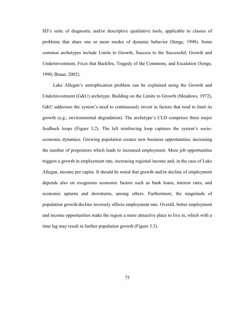
75
SD’s suite of diagnostic and/or descriptive qualitative tools, applicable to classes of
problems that share one or more modes of dynamic behavior (Senge, 1990). Some
common archetypes include Limits to Growth, Success to the Successful, Growth and
Underinvestment, Fixes that Backfire, Tragedy of the Commons, and Escalation (Senge,
1990; Braun, 2002).
Lake Allegan’s eutrophication problem can be explained using the Growth and
Underinvestment (G&U) archetype. Building on the Limits to Growth (Meadows, 1972),
G&U addresses the system’s need to continuously invest in factors that tend to limit its
growth (e.g., environmental degradation). The archetype’s CLD comprises three major
feedback loops (Figure 3.2). The left reinforcing loop captures the system’s socio-
economic dynamics. Growing population creates new business opportunities, increasing
the number of proprietors which leads to increased employment. More job opportunities
triggers a growth in employment rate, increasing regional income and, in the case of Lake
Allegan, income per capita. It should be noted that growth and/or decline of employment
depends also on exogenous economic factors such as bank loans, interest rates, and
economic upturns and downturns, among others. Furthermore, the magnitude of
population growth/decline inversely affects employment rate. Overall, better employment
and income opportunities make the region a more attractive place to live in, which with a
time lag may result in further population growth (Figure 3.3).
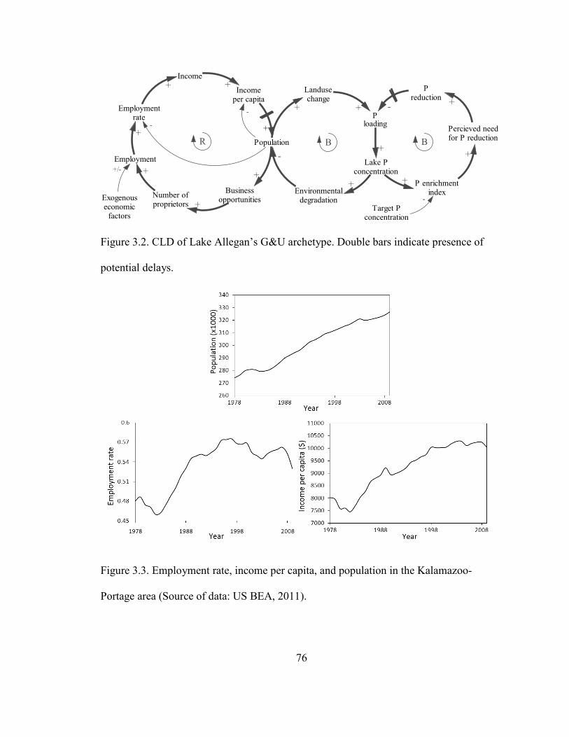
76
Figure 3.2. CLD of Lake Allegan’s G&U archetype. Double bars indicate presence of
potential delays.
Figure 3.3. Employment rate, income per capita, and population in the Kalamazoo-
Portage area (Source of data: US BEA, 2011).
Incomeper capita
Population
Employmentrate
Landusechange
Ploading
Lake Pconcentration
Environmentaldegradation
Percieved needfor P reduction
Target Pconcentration
Preduction
+
Exogenouseconomic
factors
+ +
+
+
+
R B B-
BusinessopportunitiesNumber of
proprietors
Employment
Income
+
+
+
+
+ +
-
-
+/-
-
P enrichmentindex
+
+
-
77
The socio-economic loop drives the anthropogenic environmental degradation
depicted in the middle loop. In this balancing loop, population increase brings about land
use change, in turn affecting P loadings from different land use types. In the case of Lake
Allegan, land use change will likely increase P input to the lake. Eventually, as nutrient
enrichment of the lake continues, symptoms of environmental degradation emerge,
forming a negative causal relationship with population. While eutrophication may not
have an immediate impact on upstream land owners, it directly impacts property owners
around the lake, which may lower the area’s attractiveness. The second balancing loop
(right) characterizes the measures taken to mitigate environmental degradation,
representing investment in environment. As the lake’s P concentration rises, the
discrepancy between observed and target P concentrations leads to increased perception
of the need for P reduction. P reduction plans such as TMDLs may be implemented to
reduce P loading from PSs and NPSs, helping the lake meet the prescribed water quality
target. However, in many cases, the P reduction measures will not immediately
rehabilitate the water body (Hamilton, 2012).
3.5. Model and Data Inputs
Vensim Professional 5 (Ventana Systems, 2010), one of several software packages
available for SD modeling, was used to develop and run the Lake Allegan model. A
generalized SFD of the problem, including various components of the G&U archetype, is
shown in Figure 3.4. Population and the lake TP concentration were modeled as stock
variables, whereas economic drivers, land use change, and physical processes governing
P inputs are characterized using auxiliary variables and/or equations. Nutrient reduction
78
measures are shown to target PSs and NPSs, distinctively. When simulating existing
conditions, population, income per capita, and employment were input to the model as
time series data obtained for the period of 1978-2009 from the U.S. Bureau of Economic
Analysis (US BEA, 2011). Additionally, Bureau of Labor Statistics’ Customer Price
Index calculator (US BLS, 2009) was used to obtain inflation-adjusted income in 1978
dollars. Explicit representation of the link between all different intermediate drivers
introduces multi-colinearity problems. Thus, some socio-economic variables, such as
business opportunities and number of proprietors, have been included to qualitatively
capture intermediate drivers that lead to an increase in employment as a result of
population growth. While it might be difficult to actually measure the potential increase
in business opportunities associated with more population, there is a strong correlation
between population and number of proprietors (r2 = 0.887).
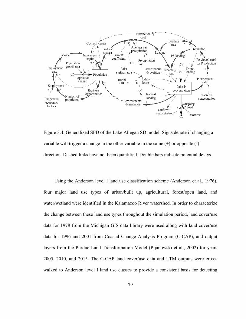
79
Figure 3.4. Generalized SFD of the Lake Allegan SD model. Signs denote if changing a
variable will trigger a change in the other variable in the same (+) or opposite (-)
direction. Dashed links have not been quantified. Double bars indicate potential delays.
Using the Anderson level I land use classification scheme (Anderson et al., 1976),
four major land use types of urban/built up, agricultural, forest/open land, and
water/wetland were identified in the Kalamazoo River watershed. In order to characterize
the change between these land use types throughout the simulation period, land cover/use
data for 1978 from the Michigan GIS data library were used along with land cover/use
data for 1996 and 2001 from Coastal Change Analysis Program (C-CAP), and output
layers from the Purdue Land Transformation Model (Pijanowski et al., 2002) for years
2005, 2010, and 2015. The C-CAP land cover/use data and LTM outputs were cross-
walked to Anderson level I land use classes to provide a consistent basis for detecting
80
changes in major land use types in the watershed. Unlike changes in forest/open land and
water/wetland, changes over time in urban/built up (rur2= 0.66) and agricultural land
(rag2= 0.88) were found to be statistically significant. The linear models best fitting the
latter land use types were used to generate land use change time series, providing land
use data for regression analyses. To satisfy land-accounting requirements, calculated
areas for urban/built up and agricultural lands were summed, and the result was
subtracted from total watershed area. The remaining area was divided between
water/wetland and forest/open land based on their respective areas in 1978. Table 3.2
summarizes the results of linear regressions between various components of the socio-
economic loop, as well as between population and urban/built up and agricultural land
use types to quantitatively establish the links illustrated in the SFD.
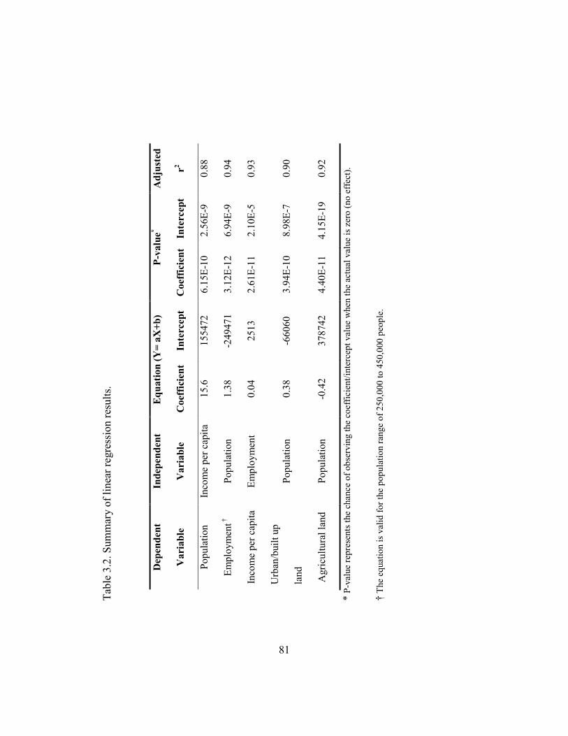
81
Tabl
e 3.
2. S
umm
ary
of li
near
regr
essi
on re
sults
.
* P-
valu
e re
pres
ents
the
chan
ce o
f obs
ervi
ng th
e co
effic
ient
/inte
rcep
t val
ue w
hen
the
actu
al v
alue
is z
ero
(no
effe
ct).
† Th
e eq
uatio
n is
val
id fo
r the
pop
ulat
ion
rang
e of
250
,000
to 4
50,0
00 p
eopl
e.
Dep
ende
nt
Inde
pend
ent
Equ
atio
n (Y
= aX
+b)
P-va
lue*
Adj
uste
d
Var
iabl
e V
aria
ble
Coe
ffic
ient
In
terc
ept
Coe
ffic
ient
In
terc
ept
r2
Popu
latio
n In
com
e pe
r cap
ita
15.6
15
5472
6.
15E-
10
2.56
E-9
0.88
Empl
oym
ent †
Po
pula
tion
1.38
-2
4947
1 3.
12E-
12
6.94
E-9
0.94
Inco
me
per c
apita
Em
ploy
men
t 0.
04
2513
2.
61E-
11
2.10
E-5
0.93
Urb
an/b
uilt
up
land
Po
pula
tion
0.38
-6
6060
3.
94E-
10
8.98
E-7
0.90
Agr
icul
tura
l lan
d Po
pula
tion
-0.4
2 37
8742
4.
40E-
11
4.15
E-19
0.
92
82
Other data requirements of the Lake Allegan SD model include average hydrologic
conditions, P loading characteristics of PSs and NPSs, and the lake’s physiographic
attributes that contribute to in-lake processes. Average quarterly precipitation data for
Southwestern Michigan were obtained from National Oceanic and Atmospheric
Administration (NOAA). Net average annual precipitation was calculated as the
difference between precipitation and evapotranspiration, which was assumed to be 50%
of precipitation (Webster et al., 1995). Surface runoff is assumed to be the key transport
mechanism for P loads from land-based NPSs. Runoff coefficients for different land use
types within Lake Allegan drainage area estimated from pervious and/or imperviousness
of the terrain were applied to calculate the runoff (eq.3.1) (Kieser and Associates, 2001).
Additionally, P loading rates estimated for the neighboring Rouge River watershed in
Southeast, MI, were applied to the Lake Allegan SD model. These loading rates were
determined using representative dry-weather field samples of storm water pollutants
collected from over fifty sampling stations (Cave et al., 1996). Reported values of
sediment burial rate in the Kalamazoo River system are in the range of 1.4x10⁻⁷ to
4.0x10⁻⁷ m/min (MDNR, 1987). The upper bound of this range was used in eq.3.2 to
characterize nutrient loss due to in-lake processes. NPS loads from immediate drainage
areas and atmospheric deposition have collectively been estimated at 154 kg/month for
April through September (Heaton, 2001). Finally, discharge data was obtained from
Fennville USGS gauging station at Lake Allegan’s outlet, and outflow P concentration
was assumed to be equal to the P concentration of the completely mixed lake. Table 3.3
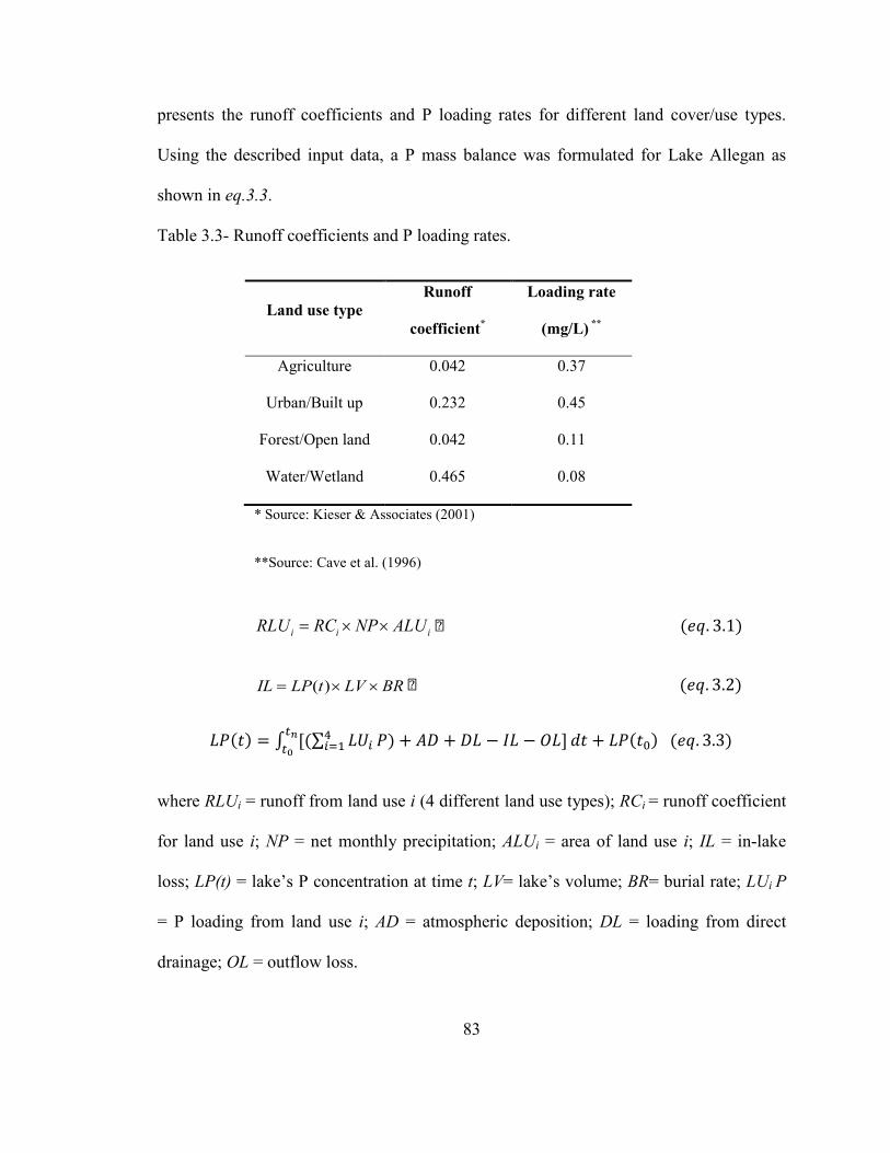
83
presents the runoff coefficients and P loading rates for different land cover/use types.
Using the described input data, a P mass balance was formulated for Lake Allegan as
shown in eq.3.3.
Table 3.3- Runoff coefficients and P loading rates.
Land use type Runoff
coefficient*
Loading rate
(mg/L) **
Agriculture 0.042 0.37 Urban/Built up 0.232 0.45
Forest/Open land 0.042 0.11 Water/Wetland 0.465 0.08
* Source: Kieser & Associates (2001)
**Source: Cave et al. (1996)
i i iRLU RC NP ALU= × × � (𝑒𝑞. 3.1)
( )IL LP t LV BR= × × � (𝑒𝑞. 3.2)
𝐿𝑃(𝑡) = ∫ [(∑ 𝐿𝑈𝑖4𝑖=1
𝑡𝑛𝑡0
𝑃) + 𝐴𝐷 + 𝐷𝐿 − 𝐼𝐿 − 𝑂𝐿]𝑑𝑡 + 𝐿𝑃(𝑡0) (𝑒𝑞. 3.3)
where RLUi = runoff from land use i (4 different land use types); RCi = runoff coefficient
for land use i; NP = net monthly precipitation; ALUi = area of land use i; IL = in-lake
loss; LP(t) = lake’s P concentration at time t; LV= lake’s volume; BR= burial rate; LUi P
= P loading from land use i; AD = atmospheric deposition; DL = loading from direct
drainage; OL = outflow loss.
84
3.6. Model Verification
The Lake Allegan model’s performance was evaluated using two sets of tests
available for verification of SD models, namely model structure and behavior tests. First,
tests of model structure were performed including structure verification, parameter
verification, extreme conditions, and dimensional consistency (Forrester and Senge,
1980; Sterman, 2000). In the structure verification test, the developed CLD and SFD
were analyzed to ensure that the proposed underlying structure (i.e., interactions between
the socio-economic loop, land use change, and the lake’s P input and output) accounts for
the main processes driving the lake’s TP concentration. The purpose of parameter
verification test is to verify that parameter values are consistent with observations of the
real system. The extreme conditions test was performed to investigate the impact of
extremely large or small nutrient inputs on the TP concentration. Finally, dimensional
consistency of the model’s auxiliary equations and stocks was examined.
In the second step of evaluating model performance, tests of model behavior were
carried out. Figure 3.5 shows the plot of simulated growing season TP concentration,
along with the 95% confidence bound and the lake’s average growing season TP
concentration (dots) measured during the period of 1998 through 2008 (Kieser and
Associates, 2011). This figure has been produced based on a Monte Carlo simulation
approach for accommodating the effects of parameter variability in TMDL studies (Gelda
et al., 2001). The most critical parameters impacting Lake Allegan’s P concentration are
runoff coefficients and P loadings from different land use types, especially from
agricultural and urban and built up areas. Therefore, a Monte Carlo simulation was
performed by running thousand simulations to sample runoff coefficients between -10%
85
and +10% of the applied coefficients, and P loads between -20% and +20% of the best-
estimate average loads.
A series of behavior reproduction tests including symptom generation, frequency
generation, behavior characteristic, and behavior sensitivity tests were done to evaluate
how well the model generates observed behavior (Forrester and Senge, 1980; Sterman,
2000; Simonovic, 2009). The model generates the primary symptom of eutrophication
reasonably well by showing that the peak of TP concentration occurs around mid-
growing season. Likewise, the model passes the frequency generation test by capturing
the seasonality of fluctuations in the TP concentration. The cyclical behavior of the
simulated TP concentration can be explained by considering the cyclical pattern of
precipitation and outflow time series (Figure 3.6). In addition, the variability and
uncertainties due to timing and frequency of TP measurements are a source of mismatch
between simulated and observed values. As illustrated in Figures 3.5 and 3.6, the
simulated TP mimics the local hydrologic behavior (i.e., peaks of precipitation and
outflow occurring during the growing season). Finally, sensitivity analysis was
performed by applying plausible shifts to model parameters such as runoff coefficients
and nutrient loading rates for different land use types to ensure the generated behavior
does not change dramatically.
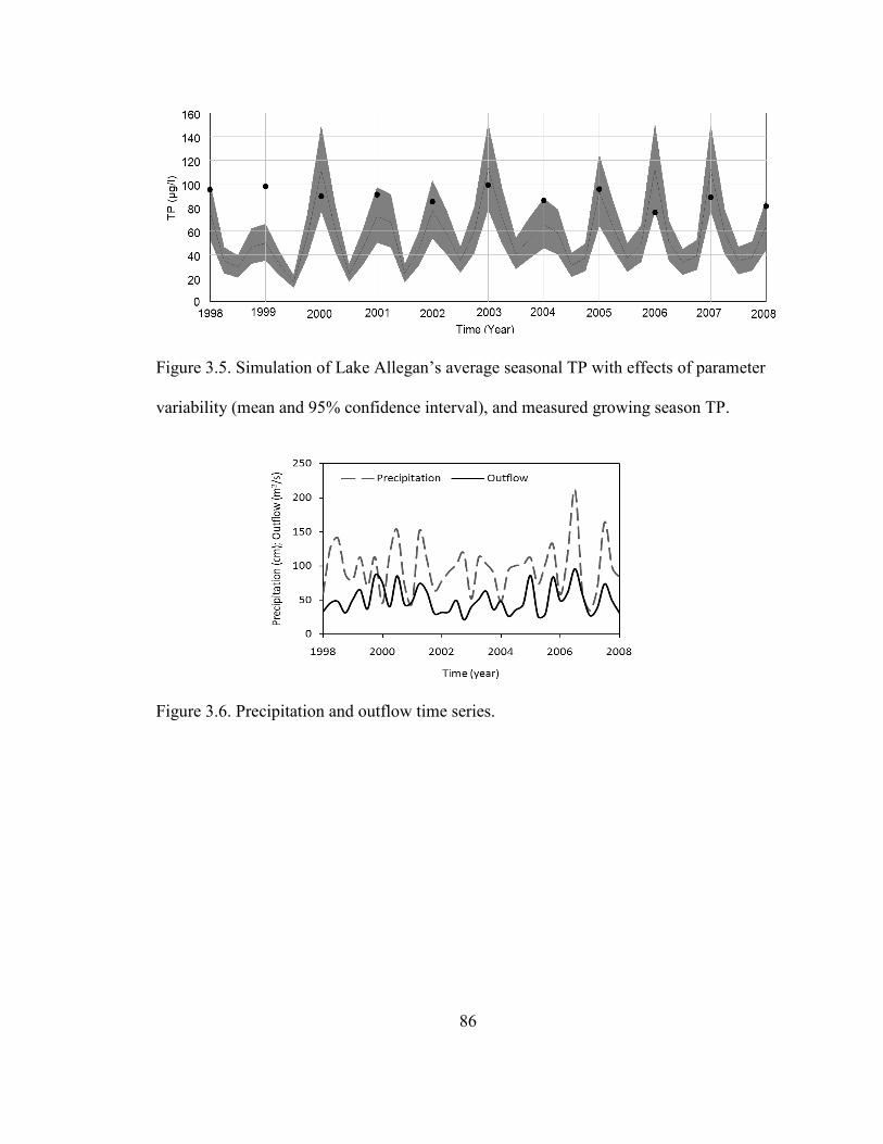
86
Figure 3.5. Simulation of Lake Allegan’s average seasonal TP with effects of parameter
variability (mean and 95% confidence interval), and measured growing season TP.
Figure 3.6. Precipitation and outflow time series.
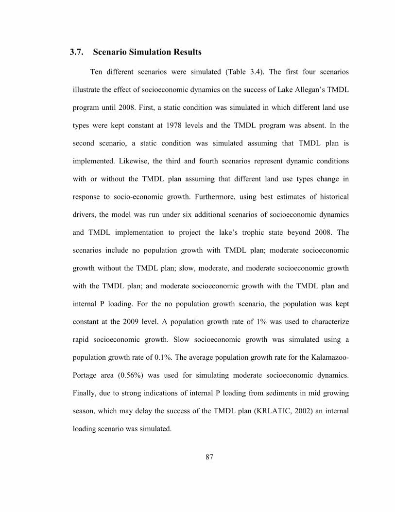
87
3.7. Scenario Simulation Results
Ten different scenarios were simulated (Table 3.4). The first four scenarios
illustrate the effect of socioeconomic dynamics on the success of Lake Allegan’s TMDL
program until 2008. First, a static condition was simulated in which different land use
types were kept constant at 1978 levels and the TMDL program was absent. In the
second scenario, a static condition was simulated assuming that TMDL plan is
implemented. Likewise, the third and fourth scenarios represent dynamic conditions
with or without the TMDL plan assuming that different land use types change in
response to socio-economic growth. Furthermore, using best estimates of historical
drivers, the model was run under six additional scenarios of socioeconomic dynamics
and TMDL implementation to project the lake’s trophic state beyond 2008. The
scenarios include no population growth with TMDL plan; moderate socioeconomic
growth without the TMDL plan; slow, moderate, and moderate socioeconomic growth
with the TMDL plan; and moderate socioeconomic growth with the TMDL plan and
internal P loading. For the no population growth scenario, the population was kept
constant at the 2009 level. A population growth rate of 1% was used to characterize
rapid socioeconomic growth. Slow socioeconomic growth was simulated using a
population growth rate of 0.1%. The average population growth rate for the Kalamazoo-
Portage area (0.56%) was used for simulating moderate socioeconomic dynamics.
Finally, due to strong indications of internal P loading from sediments in mid growing
season, which may delay the success of the TMDL plan (KRLATIC, 2002) an internal
loading scenario was simulated.
88
Table 3.4. Simulation scenarios.
Scenario Description Abbreviation
S1: Static condition without TMDL
Land use fixed at 1978 levels SC without TMDL
S2: Static condition with TMDL
Land use fixed at 1978 levels SC with TMDL
S3: Dynamic condition without TMDL
Land use changed due to socioeconomic growth
DC without TMDL
S4: Dynamic condition with TMDL
Land use changed due to socioeconomic growth
DC with TMDL
S5: No population growth without TMDL
Population fixed at 2008 level NPG without TMDL
S6: Moderate population growth without TMDL
Socioeconomic loop driven by 0.56% population growth
MPG without TMDL
S7: Slow population growth with TMDL
Socioeconomic loop driven by 0.1% population growth
SPG with TMDL
S8: Rapid population growth with TMDL
Socioeconomic loop driven by 1% population growth
RPG with TMDL
S9: Moderate population growth with TMDL
Socioeconomic loop driven by 0.56% population growth
MPG with TMDL
S10: Moderate population growth with TMDL and internal P loading
Same as scenario 9, additional linearly decreasing load applied to the period of 2010-2020
MPG with TMDL & IL
Simulation results for the first four scenarios (S1 through S4) suggest that land use
change associated with socioeconomic growth leads to greater lake P concentrations, due
to higher incoming loads from former agricultural lands that are transformed to urban and
built up (Figure 3.7). Thus, failing to incorporate the noted long-term P load dynamics in
the TMDL plan may cause an overestimation of reduction in lake P concentration. For
example, a thirty-year simulation period (1978-2008) for Lake Allegan shows that lake P
concentrations for the case of dynamic conditions with the TMDL plan may be more than
10% greater than under static conditions. Furthermore, reducing P input from NPSs is a
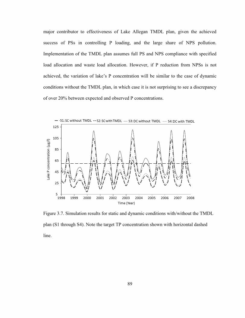
89
major contributor to effectiveness of Lake Allegan TMDL plan, given the achieved
success of PSs in controlling P loading, and the large share of NPS pollution.
Implementation of the TMDL plan assumes full PS and NPS compliance with specified
load allocation and waste load allocation. However, if P reduction from NPSs is not
achieved, the variation of lake’s P concentration will be similar to the case of dynamic
conditions without the TMDL plan, in which case it is not surprising to see a discrepancy
of over 20% between expected and observed P concentrations.
Figure 3.7. Simulation results for static and dynamic conditions with/without the TMDL
plan (S1 through S4). Note the target TP concentration shown with horizontal dashed
line.
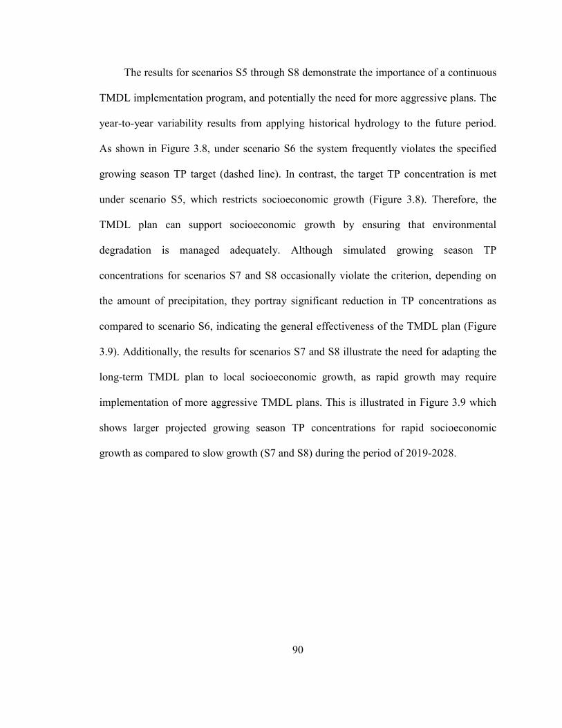
90
The results for scenarios S5 through S8 demonstrate the importance of a continuous
TMDL implementation program, and potentially the need for more aggressive plans. The
year-to-year variability results from applying historical hydrology to the future period.
As shown in Figure 3.8, under scenario S6 the system frequently violates the specified
growing season TP target (dashed line). In contrast, the target TP concentration is met
under scenario S5, which restricts socioeconomic growth (Figure 3.8). Therefore, the
TMDL plan can support socioeconomic growth by ensuring that environmental
degradation is managed adequately. Although simulated growing season TP
concentrations for scenarios S7 and S8 occasionally violate the criterion, depending on
the amount of precipitation, they portray significant reduction in TP concentrations as
compared to scenario S6, indicating the general effectiveness of the TMDL plan (Figure
3.9). Additionally, the results for scenarios S7 and S8 illustrate the need for adapting the
long-term TMDL plan to local socioeconomic growth, as rapid growth may require
implementation of more aggressive TMDL plans. This is illustrated in Figure 3.9 which
shows larger projected growing season TP concentrations for rapid socioeconomic
growth as compared to slow growth (S7 and S8) during the period of 2019-2028.
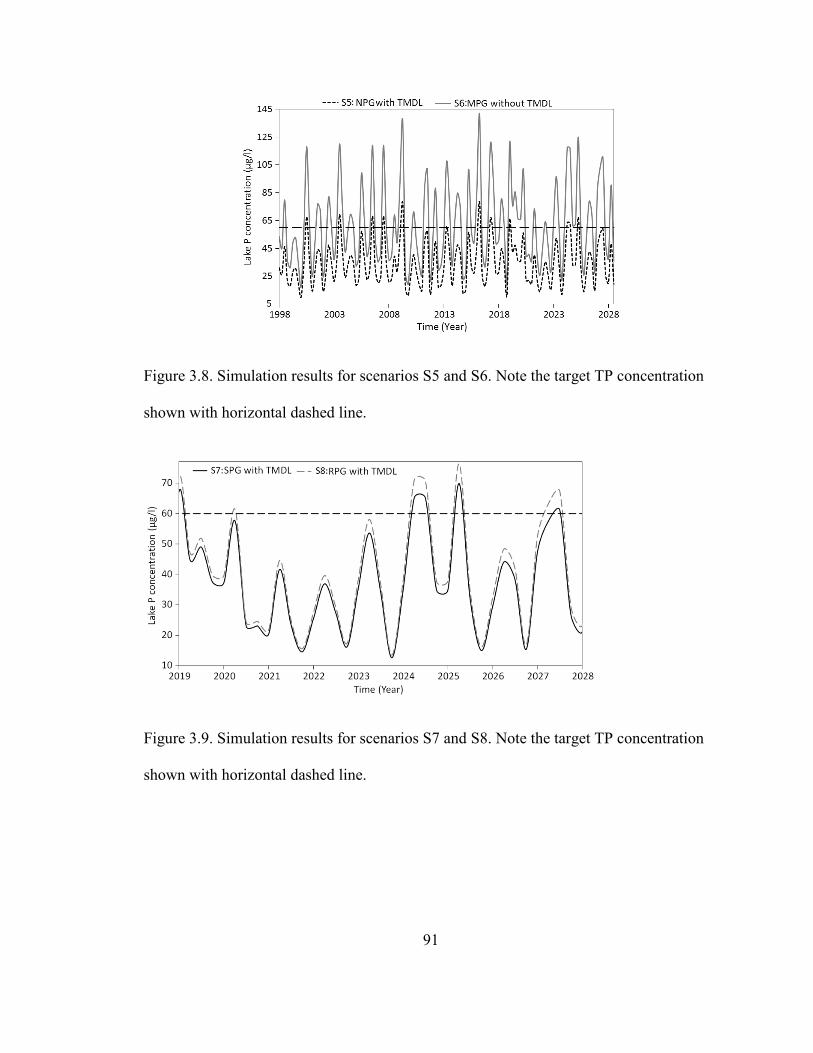
91
Figure 3.8. Simulation results for scenarios S5 and S6. Note the target TP concentration
shown with horizontal dashed line.
Figure 3.9. Simulation results for scenarios S7 and S8. Note the target TP concentration
shown with horizontal dashed line.
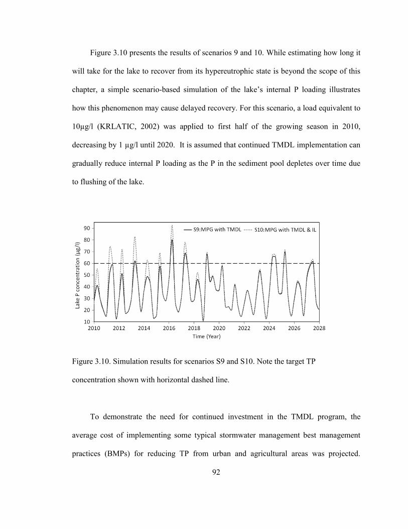
92
Figure 3.10 presents the results of scenarios 9 and 10. While estimating how long it
will take for the lake to recover from its hypereutrophic state is beyond the scope of this
chapter, a simple scenario-based simulation of the lake’s internal P loading illustrates
how this phenomenon may cause delayed recovery. For this scenario, a load equivalent to
10µg/l (KRLATIC, 2002) was applied to first half of the growing season in 2010,
decreasing by 1 µg/l until 2020. It is assumed that continued TMDL implementation can
gradually reduce internal P loading as the P in the sediment pool depletes over time due
to flushing of the lake.
Figure 3.10. Simulation results for scenarios S9 and S10. Note the target TP
concentration shown with horizontal dashed line.
To demonstrate the need for continued investment in the TMDL program, the
average cost of implementing some typical stormwater management best management
practices (BMPs) for reducing TP from urban and agricultural areas was projected.
93
Significant variability in the cost of BMPs and their effectiveness in removing TP from
urban rainwater and farmland runoff has been discussed in the literature (e.g., Withers
and Jarvis 1998; Weiss et al. 2007). Ryding and Rast (1989) provide an estimate of cost-
effectiveness of BMPs for removing NPS P loads from agricultural areas in the Lake Erie
Basin. They have reported that increased winter crop cover, spring tilling, improved
pasture management, critical source area protection, gradient terracing, and grass
waterways may provide 40% P removal at an average cost of 174 $/kg P saved. This
value was used as the cost of TMDL implementation in agricultural areas. Furthermore,
Kieser and Associates (2005) report BMP costs and effectiveness for implementation in
Southwestern Michigan. The cost of a combination of wet retention ponds, vegetated
swales, and bioretention basins to provide 50% P removal in urban areas was estimated at
316 $/kg P saved. Using these estimates, the cost of implementing BMPs to meet water
quality standards was projected under slow, moderate, and rapid socioeconomic growth
scenarios. Figure 3.11 shows the cumulative required investment in P removal, showing
the sensitivity of investment to the level of socioeconomic growth, which in the long-run
may contribute to lack of funds for implementing an effective TMDL program.
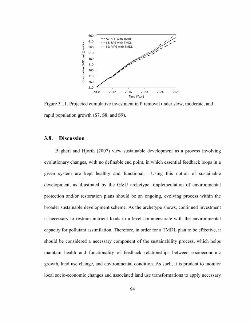
94
Figure 3.11. Projected cumulative investment in P removal under slow, moderate, and
rapid population growth (S7, S8, and S9).
3.8. Discussion
Bagheri and Hjorth (2007) view sustainable development as a process involving
evolutionary changes, with no definable end point, in which essential feedback loops in a
given system are kept healthy and functional. Using this notion of sustainable
development, as illustrated by the G&U archetype, implementation of environmental
protection and/or restoration plans should be an ongoing, evolving process within the
broader sustainable development scheme. As the archetype shows, continued investment
is necessary to restrain nutrient loads to a level commensurate with the environmental
capacity for pollutant assimilation. Therefore, in order for a TMDL plan to be effective, it
should be considered a necessary component of the sustainability process, which helps
maintain health and functionality of feedback relationships between socioeconomic
growth, land use change, and environmental condition. As such, it is prudent to monitor
local socio-economic changes and associated land use transformations to apply necessary
95
adjustments to the allowable load and waste load allocations, as well as a TMDL’s
margin of safety.
The presented results are based on the fundamental assumption that the proposed
TMDL plan for Lake Allegan is fully implemented by PSs and NPSs. In actuality,
however, it has proven difficult for NPSs to comply with the designated load allocations.
In the Lake Allegan’s TMDL plan, P reduction from NPSs is to be achieved through
voluntary cutbacks by participants, mainly from the agriculture sector (KRLATIC, 2002).
While some level of public participation and voluntary cooperation are important for the
success of management plans, applying appropriate regulations such as banning high-P
agricultural fertilizers may be necessary to avoid Tragedy of the Commons (Hardin,
1968) and free-riding (Madani and Lund, 2011). Lack of political will, leadership, funds,
and authority to enforce compliance with water quality standards are among key factors
complicating TMDL implementation. Additionally, on-going monitoring to evaluate the
effectiveness of the TMDL plan, and inform decision makers and stakeholders as to
timely progress towards water quality targets, is essential for establishing adaptive plans.
It is critical to identify funding sources for long-term TMDL programs, and
evaluate potential socio-economic impacts of TMDL implementation to guide
environmental decision making. For example, applying an environmental tax may
negatively affect economic growth, leading to reduced income per capita. However, as
shown in the CLD of the G&U archetype for Lake Allegan, improvement in
environmental conditions may compensate for reduced utility, attracting population from
areas with inferior environmental quality, and creating opportunities for socioeconomic
growth (Rephann, 2010). Therefore, effective policy for reducing the lake’s P
96
concentration in the long-run should aim to internalize environmental externalities
associated with socioeconomic growth, increase voluntary public participation in the
TMDL program, and regulate P load input to the lake from PSs and NPSs.
3.9. Conclusions
Using the Lake Allegan eutrophication problem as a case study, it is shown that
simple SD models can be developed and verified to facilitate qualitative and strategic-
level quantitative analysis of interlinked socioeconomic and biophysical subsystems.
Obtaining an accurate match between simulated and observed values is not sufficient for
verification of causal-descriptive SD models, which should help explain how the
behavior is generated. Thus, the Lake Allegan model was verified using is a semi-formal
approach involving a mix of qualitative criteria and quantitative tests focusing on the
system’s structure. The model facilitates trend identification and pattern recognition,
guiding holistic TMDL policy and long-term adaptive management in which potential
impacts of socio-economic dynamics may be partially addressed using an appropriate
margin of safety in the proposed TMDL plan. On-going monitoring campaigns can help
determine whether the proposed TMDL plan is adequate for the extant socio-economic
condition, or if there is a need for a more aggressive plan.
The principles and tools of systems thinking can improve holistic understanding of
the underlying system structure driving water quality problems. Herein the G&U system
archetype is used to explain Lake Allegan’s eutrophication problem, demonstrating the
need for continued investment to limit environmental degradation, essential for balanced
socio-economic growth. This need stems from the process-based nature of sustainable

97
development which calls for managing feedback relationships between socioeconomic
dynamics, land use change, and environmental integrity. Without appropriately capturing
these important feedback loops, TMDL plans may set overambitious water quality targets
to be achieved within an unrealistic timeframe.
98
3.10. References
Anderson, J. R., Hardy, E.E., Roach J.T., Witmer, R.E. (1976). A land use and land cover
classification system for use with remote sensor data. U.S. Geological Survey
Professional Paper 964, U.S. Geological Survey, Reston, Virginia.
Arrow, K., Bolin, B., Costanza, R., Dasgupta, P., Folke, C., Holling, C.S., Jansson, B.O.,
Levin, S., Mäler, K.G., Perrings, C.A., Pimentel, D. (1995). Economic growth,
carrying capacity, and the environment. Science 268, 520–521.
Bagheri, A., Hjorth, P. (2007). Planning for sustainable development: a paradigm shift
towards a process-based approach. Sustainable Development 15, 83–96.
Benham, B., Zeckoski, R., Yagow, G. (2008). Lessons learned from TMDL
implementation case studies. Water Practice 2(1), 1-13.
Bishop, R. (1993). Economic efficiency, sustainability and biodiversity. Ambio 22 (2-3),
69-73.
Boyd, J. (2000). Unleashing the clean water act, the promise and challenge of the TMDL
approach to water quality. Resources 139, 7-10.
Braun, W., 2002. The system archetypes. <http://wwwu.uni-klu.ac.at/gossimit/pap/sd/
wb_sysarch.pdf> (accessed on Sep. 21, 2011).
Canale, R.P., Redder, T., Swiecki, W., Whelan, G. (2010). Phosphorus budget and
remediation plan for Big Platte Lake, Michigan. Journal of Water Resources
Planning and Management 136(5), 576-586.
Cave, K., Harold, E., Quasebarth, T. (1996). Preliminary pollution loading projections for
Rouge River watershed and interim nonpoint source pollution control plan,
99
Technical Report RPO-NPS-TR07.00, Rouge River National Wet Weather
Demonstration Project, Wayne County, Michigan.
Cooke, G.D., Welch, E.B., Peterson, S.A., Newroth, P.R. (1993). Restoration and
Management of Lakes and Reservoirs. Boca Raton, Florida.
Doerr, S.M., Canale, R.P., Effler, S.W. (1996). Development and testing of a total
phosphorus model for Onondaga Lake. Lake and Reservoir Management 12(1),
141-150.
Effler, S.W., O'Donnell, S.M., Matthews, D.A., Matthews, C.M., O'Donnell, D.M., Auer,
M.T., Owens, E.M. (2002). Limnological and loading information and a
phosphorus total maximum daily load (TMDL) analysis for Onondaga Lake. Lake
and Reservoir Management 18(2), 87-108.
Ehrlich, P.R., Holdrens, J.P. (1971). The impact of population growth. Science 171,
1212–1217.
Ford, A. (1999). Modeling the environment. Island Press, Washington.
Forrester, J. (1961) Industrial dynamics. MIT Press, Cambridge.
Forrester, J. (1969) Urban dynamics. MIT Press, Cambridge.
Forrester, J.W., Senge, P.M. (1980). Tests for building confidence in system dynamics
models. In: System dynamics (Ed.). Legasto, A.A., Forrester, J.W., and Lyneis, J.
M., Amsterdam.
FWPCA (1972). Federal water pollution control act, as amended (33 U.S.C. 1151 et
seq.).
FWPCA (2002). Federal water pollution control act, as amended (33 U.S.C. 1251 et
seq.).
100
Gelda, R.K., Effler, S.W., and O’Donnell, S.M. (2001). Probabilistic model of ammonia
and toxicity status for urban lake. Journal of Water Resources Planning and
Management 127, 337–347.
Guo, H.C., Liu, L., Huang, G.H., Fuller, G.A., Zou, R., Yin, Y.Y. (2001). A system
dynamics approach for regional environmental planning and management: a study
for the Lake Erhai Basin. Environmental Management 61(1), 93–111.
Hamilton, S.K. (2012). Biogeochemical time lags may delay responses of streams to
ecological restoration. Fresh Water Biology 57, 43–57.
Hardin, G. (1968). The tragedy of the commons. Science 162, 1243-1248.
Hartig, J.H., Horvath, F.J. (1982). A preliminary assessment of Michigan's phosphorus
detergent ban. Journal Water Pollution Control Federation 54, 193-197.
Havens, K.E. Schelske, C. L. (2001). The importance of considering biological processes
when setting total maximum daily loads (TMDL) for phosphorus in shallow lakes
and reservoirs. Environmental Pollution 113, 1-9.
Heaton, S. (2001). Total maximum daily load (TMDL) for total phosphorus in Lake
Allegan. Surface Water Quality Division, Michigan Department of Environmental
Quality. Lansing, Michigan.
Hjorth, P., and Bagheri, A. (2006). Navigating towards sustainable development: a
system dynamics approach. Futures 38(1), 74–92.
Kieser and Associates (2001). Non-point source modeling of phosphorus loads in the
Kalamazoo River/Lake Allegan watershed for a total maximum daily load. Kieser
and Associates Environmental Science and Engineering, Kalamazoo, Michigan.
101
Kieser and Associates (2005). Analysis of urban stormwater best management practice
options for the St. Joseph River watershed. Prepared for: Friends of the St. Joseph
River, Kieser and Associates Environmental Science and Engineering,
Kalamazoo, Michigan.
Kieser and Associates (2011). 2010 TMDL evaluation: a look at how we are doing on
TMDL goals. Kieser and Associates Environmental Science and Engineering,
<http://kalamazooriver .net/> (accessed on Oct. 3, 2011).
KRLATIC (2002). Water quality improvement (implementation) plan for the Kalamazoo
River watershed and Lake Allegan through a phosphorus total maximum daily
load (TMDL) process. The Kalamazoo River/Lake Allegan TMDL
Implementation Committee, Kalamazoo, Michigan.
Leal Neto, A.C., Legey, L.F.L., Gonzalez-Araya, M.C., Jablonski, S. (2006). A system
dynamics model for the environmental management of the Sepetiba Bay
watershed, Brazil. Environmental Management 38(5), 879–888.
Madani, K., Lund, J.R. (2011). California's Sacramento-San Joaquin Delta Conflict: from
Cooperation to Chicken. Journal of Water Resources Planning and Management
138(2), 90-99.
Madani, K., Mariño, M.A. (2009). System dynamics analysis for managing Iran’s
Zayandeh-Rud river basin. Water Resources Management 23(11), 2163-2187.
MDEQ (1999). Loading assessments of phosphorus inputs to Lake Allegan. Staff Report,
Surface Water Quality Division, Michigan Department of Environmental Quality,
Lansing, Michigan.
102
MDNR (1987). Remedial action plan for the Kalamazoo River. Michigan Department of
Natural Resources, Bay City, Michigan.
Meadows, D.H., Meadows, D.L., Randers, J., Behrens, W.W. (1972). The limits to
growth. Universe Books, New York.
MWQS (2006). Michigan water quality standard. Water Resources Protection, Water
Bureau, Department of Environmental Quality, Lansing, Michigan.
Pijanowski, B.C., Brown, D.G., Shellito, B.A., Manik, G.A. (2002). Using neural
networks and GIS to forecast land use changes: a land transformation model.
Computers, Environment and Urban Systems 26(6), 553–575.
Rephann, T.J. (2010). Economic impacts of implementing agricultural best management
practices to achieve goals outlined in Virginia’s tributary strategy, Center for
Public Service University of Virginia, Charlottesville, Virginia.
Ryding, S.O., Rast, W. (1989). The control of eutrophication of lakes and reservoirs.
UNESCO, Paris, France.
Senge, P. (1990). The fifth discipline: the art & practice of the learning organization.
Doubleday/Currency, New York.
Shirmohammadi, A., Chaubey, I., Harmel, R.D., Bosch, D.D., Muñoz-Carpena, R.,
Dharmasri, C., Sexton, A., Arabi, M., Wolfe, M.L., Frankenberger, J., Graff, C.,
and Sohrabi., T.M. (2006). Uncertainty in TMDL models. Transaction of The
American Society of Agricultural and Biological Engineers 49(4), 1033−1049.
Simonovic, S.P. (2009). Managing water resources: methods and tools for a systems
approach. UNESCO, Paris and Earthscan James & James, London.
103
Simonovic, S.P., Fahmy, H. (1999). A new modeling approach for water resources policy
analysis. Water Resources Research 35(1), 295–304.
Sterman, J.D. (2000). Business dynamics, systems thinking and modeling for a complex
world. McGraw-Hill, Boston.
US BEA (2011). U.S. economic accounts. U.S. Bureau of Economic Analysis,
<http://www. bea.gov/index.htm> (accessed on Aug.3, 2011).
US BLS (2009). Customer price index. U.S. Bureau of Labor Statistics, < http://www.
bls.gov/cpi/cpifact8.htm> (accessed on Aug. 5, 2011).
US EPA (1975). Report on Lake Allegan, Allegan County, Michigan. Working Paper
182. U.S. Environmental Protection Agency Region V, Chicago, Illinois.
Ventana Systems (2010) User's Guide Version 5. 2010. Ventana Systems, Inc.,
<http://www. vensim.com> (accessed on Aug.13, 2011).
Vergura, J., Jones, R. (2001). The TMDL program: land use and other implications.
Drake Journal of Agricultural Law 6(2), 317.
Vezjak, M., Savsek, T., Stuhler, E.A. (1998). System dynamics of eutrophication
processes in lakes. European Journal of Operations Research, 109(2), 442-451.
Vondracek, B., Zimmerman, J.K.H., Westra, J.V. (2003). Setting an effective TMDL:
sediment loading and effects of suspended sediment on fish. Journal of American
Water Resources Association 39(5), 1005–1015.
Webster, J.R., Wallace, J.B., Benfield, E.F. (1995). Organic processes in streams of the
eastern United States. In: Cushing, C.E., Cummins, K.W., and Minshall, G.W.
(eds), Ecosystems of the world, 22, River and stream ecosystems. Elsevier,
Amsterdam, 117-187.
104
Weiss, P.T., Gulliver, J.S., Erickson, A.J. (2007). Cost and pollutant removal of storm-
water treatment practices. Journal of Water Resources Planning and Management
133, 218–229.
Winz, I., Brierley, G., Trowsdale, S. (2009). The use of system dynamics simulation in
water resource management. Water Resources Management 23(7), 1301–1323.
Withers, P.J.A., Jarvis, G.C. (1998). Mitigation options for diffuse P loss to water. Soil
Use and Management 14, 186-192.
Wuycheck, J. (1998). Water quality and pollution control in Michigan. Surface Water
Quality Division, Report No. MI/DEQ/SWQ-98/030, Michigan 305(b) Report,
Michigan Department of Environmental Quality, Lansing, Michigan.
105
Chapter 4 - A high-level simulation-optimization framework for non-point source phosphorus load reduction in the Kalamazoo River watershed (Michigan, USA)4 4.1. Abstract
The US Clean Water Act has been reasonably successful in point source (PS)
pollution abatement through technology-based end-of-pipe regulation. However, total
maximum daily load (TMDL) programs stipulated under the Clean Water Act fail to
provide guidance for systematic approaches to evaluating the tradeoffs associated with
alternative non-point source (NPS) pollutant abatement strategies. Furthermore, TMDL
programs do not typically account for socioeconomic and biophysical feedbacks and
uncertainties in future conditions affecting long-term attainability of the desired water
quality target. Using the eutrophic Lake Allegan in Michigan as a case study, this chapter
presents a high-level simulation-optimization framework, comprising system dynamics
simulation and a best management practice (BMP) optimization model, for NPS total
phosphorus (TP) reduction in the Kalamazoo River watershed. Long-term adequacy of
the watershed’s TMDL plan and tradeoffs between BMP implementation cost and
reliability of meeting the lake’s TP concentration target are investigated. The results
suggest that NPS TP load reduction through agricultural BMPs such as buffer strips and
conservation tillage should be given priority, supplemented by urban grassed swale with
buffer strips and storage practices (detention and retention basins). The NPS pollution
abatement required for achieving the lake’s TP concentration target with high reliability
4 This chapter is being considered for publication as Mirchi, A., Watkins, D.W. Jr. A high-level simulation-optimization framework for non-point source phosphorus load reduction in the Kalamazoo River watershed. Science of the Total Environment.
106
using agricultural BMPs can be prohibitively costly to agricultural producers, indicating
the potential need for government intervention, as well as potential for environmental
offset programs. Furthermore, although the lake’s TP concentration is primarily governed
by intra- and inter-annual hydrologic variability, the projected socioeconomic growth in
the watershed is expected to negatively affect the reliability of meeting the water quality
goal. Periodic updating of the TMDL plan can increase reliability, and result in
potentially significant cost savings by improving the timing of the required BMP
investments.
4.2. Introduction
Human intervention is necessary for maintaining environmental integrity by
mitigating anthropogenic environmental degradation associated with socioeconomic
growth. The need for the human intervention can be explained by the Growth and
Underinvestment (G&U) system archetype (Senge, 1990), which builds on the well-
known Limits to Growth archetype (Meadows et al., 1972). In an environmental context,
the G&U archetype portrays how inadequate investment in maintaining environmental
quality may activate socio-ecological feedbacks that, ultimately, will limit the system’s
growth. One example of the feedbacks threatening to limit the growth of socio-
ecological systems is the widespread algae blooms in eutrophic lakes (e.g., Smith, 2003;
Paerl et al., 2011; Michalak et al., 2013), indicating unsustainable development. There is
an evident need for systematic initiatives and aggressive policies to mitigate degradation
of aquatic systems (Booth and Jackson, 1997; Carpenter et al., 1998).
107
In the US, the Clean Water Act (CWA) of 1972 (FWPCA, 1972) and the
subsequent amendments (e.g., the CWA amendment of 2002 (FWPCA, 2002)) provide a
legal framework for human intervention to maintain environmental integrity of the
nation’s water bodies. The CWA triggered efforts to determine impairment of water
bodies and recommend ways to address the issue(s), although, in some cases, lack of
clear impairment listing and delisting methodologies has caused inconsistent impairment
determination in different states (Keller and Cavallaro, 2008). The states must quantify
the total maximum daily load (TMDL) of a pollutant that a water body can receive
without violating specified water quality standards (FWPCA, 2002). Point sources (PS),
non-point sources (NPS) and natural background nutrient loads (e.g., mineralization of
native organic matter) are characterized, and a factor of safety is warranted to account for
potential lack of knowledge. The statute has brought about significant environmental
improvements in the riverine areas (Boyd, 2000). However, more than four decades after
its passage, the US is far from having healthy aquatic communities, as 55% of the
country’s rivers and streams are in poor biological condition, mostly due to excessive
amounts of phosphorus and nitrogen (US EPA 2013, P11). Likewise, of 39% of the
assessed lakes and reservoirs, excluding the Great Lakes, 64% were “impaired or not
clean enough to support their designated uses, such as fishing and swimming” (US EPA
2009, P16).
The biophysical aspects of watershed processes and NPS pollutants driving
anthropogenic eutrophication have been the subject of extensive research (e.g., Carpenter
et al., 1998; Gburek et al., 2000; Haygarth et al., 2005; Heathwaite et al., 2005; Rao et al.,
2009), providing valuable insights for implementation of best management practices
108
(BMPs) for pollutant reduction (e.g., Veith et al., 2003; Gitau et al., 2004; Zhen et al.,
2004; Hsieh and Yang, 2007; Panagopoulos et al., 2011; Lee et al., 2012; Giri et al.,
2012). In the US, PS pollution abatement has been reasonably successful due to the
relative ease of command-and-control, technology-based end-of-pipe regulation, whereas
urban (e.g., combined sewer overflows, runoff from lawns, and septic tanks) and
agricultural (e.g., excess fertilizer) NPS pollutant load reduction is much more
challenging (Sharpley et al., 1994; Boyd, 2000). A variety of BMPs have been used for
TMDL implementation in urban settings (Tsihrintzis and Hamid, 1997; Sample et al.,
2003; Weiss et al., 2007) and agricultural areas (Sharpley et al., 1994; Bottcher et al.,
1995; Withers and Jarvis, 1998; Kleinman et al., 2011). BMPs that reduce total
phosphorous (TP) loads (e.g., buffer strips, tillage practices, and basin practices) have
received particular attention, as this nutrient is usually the limiting factor for
eutrophication of fresh water aquatic systems (Lee et al., 1978; Sharpley et al., 1994;
Correll, 1998; Mainstone and Parr, 2002).
A systematic approach to TMDL implementation, including cost-effective NPS
pollution reduction, needs further investigation. The approach should consider the
potential impacts of socioeconomic growth, associated biophysical changes, and
hydrologic variability on the tradeoffs between TP abatement cost and reliability of
meeting the desired water quality goal. Many researchers have focused on watershed
processes to demonstrate the tradeoffs between BMP cost and pollutant load reduction at
the watershed scale (e.g., Milon, 1987; Arabi et al., 2006; Maringanti et al., 2009;
Rodriguez et al., 2011, Panagopoulos et al., 2012), as well as the farm scale (Gitau et al.,
2004; Gooday et al., in press). Fewer studies have recommended optimal eutrophication
109
control policies using macroeconomic and ecologic approaches (e.g., Hein, 2006; Deng et
al., 2011). Hein (2006) developed an ecological-economic model to study cost-benefit
implications of optimal eutrophication control policies for improving ecosystem
functions of a shallow lake. Deng et al. (2011) presented a macroeconomic model of cost-
effective policies to balance regional economic growth with pollutant reduction to
address the eutrophication of Poyang Lake in China. Accounting for the socioeconomic
and biophysical feedbacks driving eutrophication will help TMDL planners to avoid the
pitfall of setting overly ambitious water quality targets or unrealistic time frames to
achieve those targets (Mirchi and Watkins, in press).
Furthermore, TMDL programs have not typically provided systematic guidance on
alternative mitigation methods and long-term attainability of the target. Often, the scope
of the programs is practically limited to identifying the main pollutant of concern,
quantifying existing pollutant loads, and specifying target water quality standards based
on the available guidelines (e.g., US EPA, 1991). However, a comprehensive TMDL
process to address the NPS pollution requires a number of other important components to
facilitate effective policies. The Chesapeake Bay TMDL program has applied a more
holistic environmental systems analysis approach to TMDL planning as compared with
typical programs (Schwartz, 2010; US EPA, 2012). Environmental systems analysis
techniques should be systematically incorporated in TMDL studies in order to explore a
potential set of “optimal” strategies for meeting the target. Moreover, the long-term
attainability of the target using the desired mitigation method in the presence of dynamic
system-wide drivers (e.g., socioeconomic) and associated feedbacks (e.g., land use
change) should be investigated. The insights obtained from these steps will provide a
110
good basis for identifying effective mitigation policies and practices whose success can
be evaluated through adequate monitoring campaigns.
The objective of this chapter is to investigate the noted components of the proposed
TMDL planning paradigm using a high-level simulation-optimization framework for
watershed-scale NPS TP reduction in the Kalamazoo River watershed, Michigan. A
system dynamics (SD) simulation model is used in conjunction with a screening-level
optimization model to find a set of least-cost BMPs for TP load reduction. Using the
eutrophic Lake Allegan as a case study, this chapter draws insights into 1) the long-term
(30 years) adequacy of the proposed TMDL; 2) the tradeoffs between NPS BMP
implementation cost and reliability of meeting water quality target; and 3) the potential
impacts of the watershed’s socioeconomic growth on attainment of the target. The next
section presents the methodology, including the SD model and the optimization model
for finding the least-cost BMP set. Section 3 provides the results, a discussion of the
existing challenges of TMDL programs, and the implications of potential policies for
BMP implementation. Section 4 concludes the chapter.
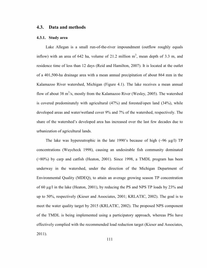
111
4.3. Data and methods
4.3.1. Study area
Lake Allegan is a small run-of-the-river impoundment (outflow roughly equals
inflow) with an area of 642 ha, volume of 21.2 million m3, mean depth of 3.3 m, and
residence time of less than 12 days (Reid and Hamilton, 2007). It is located at the outlet
of a 401,500-ha drainage area with a mean annual precipitation of about 864 mm in the
Kalamazoo River watershed, Michigan (Figure 4.1). The lake receives a mean annual
flow of about 38 m3/s, mostly from the Kalamazoo River (Wesley, 2005). The watershed
is covered predominately with agricultural (47%) and forested/open land (34%), while
developed areas and water/wetland cover 9% and 7% of the watershed, respectively. The
share of the watershed’s developed area has increased over the last few decades due to
urbanization of agricultural lands.
The lake was hypereutrophic in the late 1990’s because of high (~96 µg/l) TP
concentrations (Wuycheck 1998), causing an undesirable fish community dominated
(>80%) by carp and catfish (Heaton, 2001). Since 1998, a TMDL program has been
underway in the watershed, under the direction of the Michigan Department of
Environmental Quality (MDEQ), to attain an average growing season TP concentration
of 60 µg/l in the lake (Heaton, 2001), by reducing the PS and NPS TP loads by 23% and
up to 50%, respectively (Kieser and Associates, 2001; KRLATIC, 2002). The goal is to
meet the water quality target by 2015 (KRLATIC, 2002). The proposed NPS component
of the TMDL is being implemented using a participatory approach, whereas PSs have
effectively complied with the recommended load reduction target (Kieser and Associates,
2011).
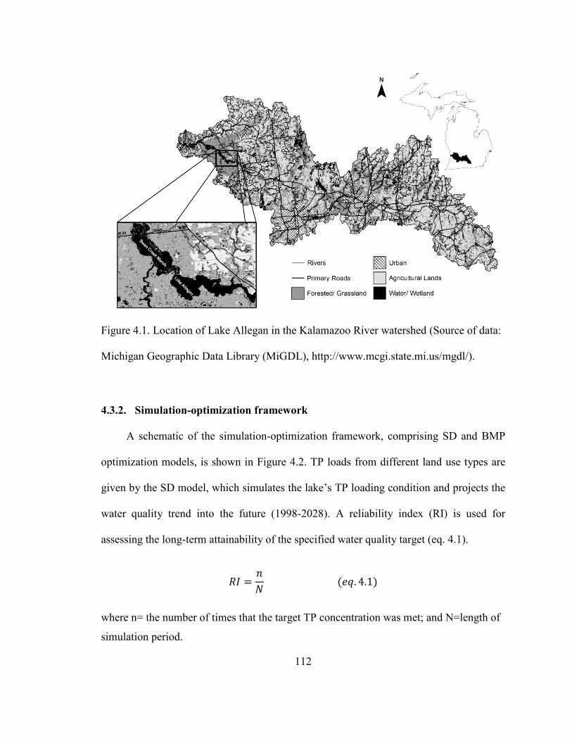
112
Figure 4.1. Location of Lake Allegan in the Kalamazoo River watershed (Source of data:
Michigan Geographic Data Library (MiGDL), http://www.mcgi.state.mi.us/mgdl/).
4.3.2. Simulation-optimization framework
A schematic of the simulation-optimization framework, comprising SD and BMP
optimization models, is shown in Figure 4.2. TP loads from different land use types are
given by the SD model, which simulates the lake’s TP loading condition and projects the
water quality trend into the future (1998-2028). A reliability index (RI) is used for
assessing the long-term attainability of the specified water quality target (eq. 4.1).
𝑅𝐼 =𝑛𝑁
(𝑒𝑞. 4.1)
where n= the number of times that the target TP concentration was met; and N=length of
simulation period.
113
The TP loads obtained from the SD model are input to the optimization model to
identify the least-cost BMP set. The outcomes of the optimization model are evaluated
using the SD model to produce tradeoff curves with consideration of feedbacks under
different socioeconomic growth scenarios. This is done by using the post-BMP TP loads
in the SD model in order to examine the effectiveness of the least-cost BMP set. Higher
values of RI may be obtained through considering more stringent mean TP concentration
requirements (<60µg/l) in the deterministic optimization model. Comparison of the
projected water quality trends for the two cases of with and without BMPs provides
insights as to adequacy of the BMP set for long-term attainment of the water quality
target.
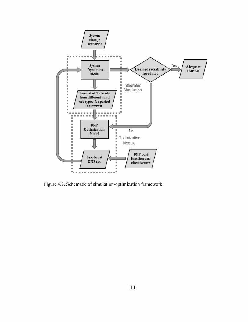
114
Figure 4.2. Schematic of simulation-optimization framework.
115
4.3.3. System dynamics simulation
System dynamics simulation (Forrester 1961 and 1969; Ford 1999; Sterman 2000)
is a method for operationalizing systems thinking (Senge 1990), facilitating holistic water
resources modeling (Simonovic 2009; Mirchi et al., 2012). Winz et al. (2009) and Mirchi
et al. (2012) reviewed system dynamics applications to water resources problems, as well
as the pros and cons of the approach. Mirchi and Watkins (in press) used the G&U
archetype with three main feedback loops, i.e., socioeconomic, biophysical, and human
intervention to explain system-wide processes governing the anthropogenic
eutrophication of Lake Allegan. A high-level system dynamics model was developed to
simulate the changes over time in the socioeconomic loop, driving the land use change,
and TP loading of the lake. A generalized stock-and-flow diagram of the model was
presented in chapter three (Figure 3.4). The model is used in this study to simulate the
effect of NPS TP load reduction using least-cost urban and agricultural BMPs. The model
and data inputs, provided in greater detail in Mirchi and Watkins (in press), are described
here.
Time series data (1978-2009) for population, income per capita, and employment
were obtained from the U.S. Bureau of Economic Analysis (US BEA 2011).
Additionally, Bureau of Labor Statistics’ Customer Price Index calculator (US BLS
2009) was used to obtain inflation-adjusted income. Using available land use data from
Michigan GIS data library for 1975, Coastal Change Analysis Program (C-CAP) for 1996
and 2001, and Purdue Land Transformation Model (Pijanowski et al. 2002) for 2005,
2010, 2015, linear regression models best fitting the trend of change for urban/built up
and agricultural lands were developed to generate a land use time series. Statistically
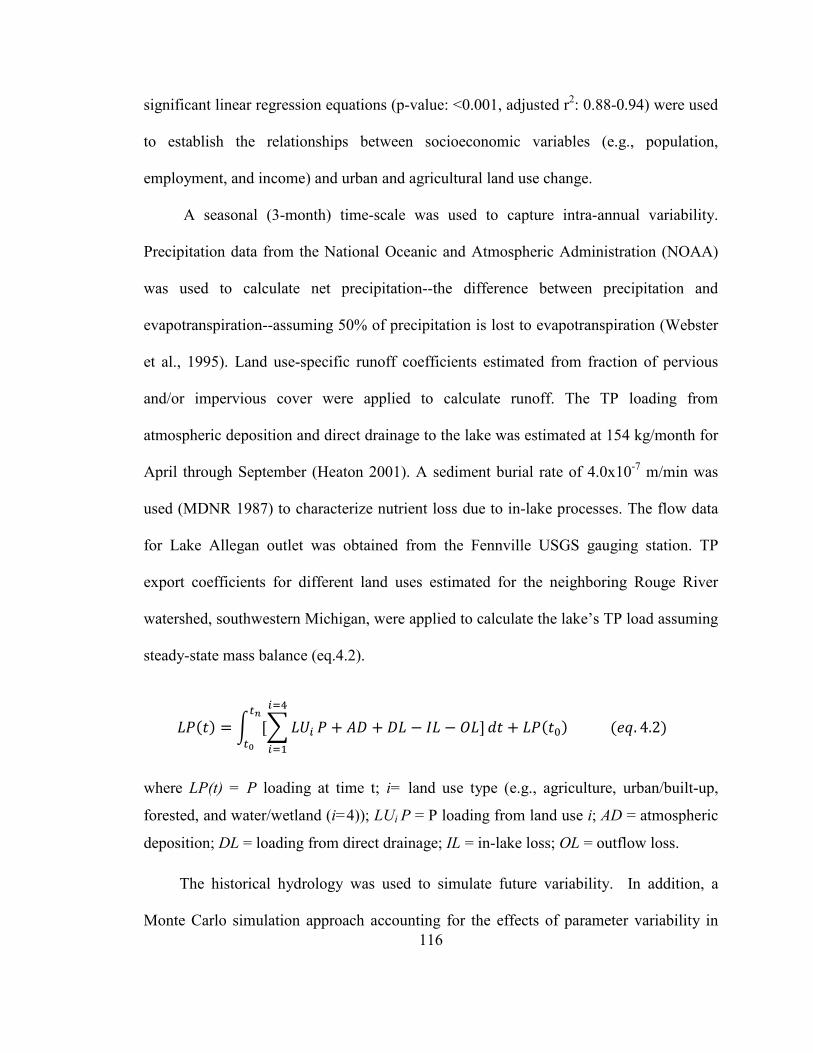
116
significant linear regression equations (p-value: <0.001, adjusted r2: 0.88-0.94) were used
to establish the relationships between socioeconomic variables (e.g., population,
employment, and income) and urban and agricultural land use change.
A seasonal (3-month) time-scale was used to capture intra-annual variability.
Precipitation data from the National Oceanic and Atmospheric Administration (NOAA)
was used to calculate net precipitation--the difference between precipitation and
evapotranspiration--assuming 50% of precipitation is lost to evapotranspiration (Webster
et al., 1995). Land use-specific runoff coefficients estimated from fraction of pervious
and/or impervious cover were applied to calculate runoff. The TP loading from
atmospheric deposition and direct drainage to the lake was estimated at 154 kg/month for
April through September (Heaton 2001). A sediment burial rate of 4.0x10⁻⁷ m/min was
used (MDNR 1987) to characterize nutrient loss due to in-lake processes. The flow data
for Lake Allegan outlet was obtained from the Fennville USGS gauging station. TP
export coefficients for different land uses estimated for the neighboring Rouge River
watershed, southwestern Michigan, were applied to calculate the lake’s TP load assuming
steady-state mass balance (eq.4.2).
𝐿𝑃(𝑡) = � [�𝐿𝑈𝑖
𝑖=4
𝑖=1
𝑡𝑛
𝑡0𝑃 + 𝐴𝐷 + 𝐷𝐿 − 𝐼𝐿 − 𝑂𝐿]𝑑𝑡 + 𝐿𝑃(𝑡0) (𝑒𝑞. 4.2)
where LP(t) = P loading at time t; i= land use type (e.g., agriculture, urban/built-up,
forested, and water/wetland (i=4)); LUi P = P loading from land use i; AD = atmospheric
deposition; DL = loading from direct drainage; IL = in-lake loss; OL = outflow loss.
The historical hydrology was used to simulate future variability. In addition, a
Monte Carlo simulation approach accounting for the effects of parameter variability in
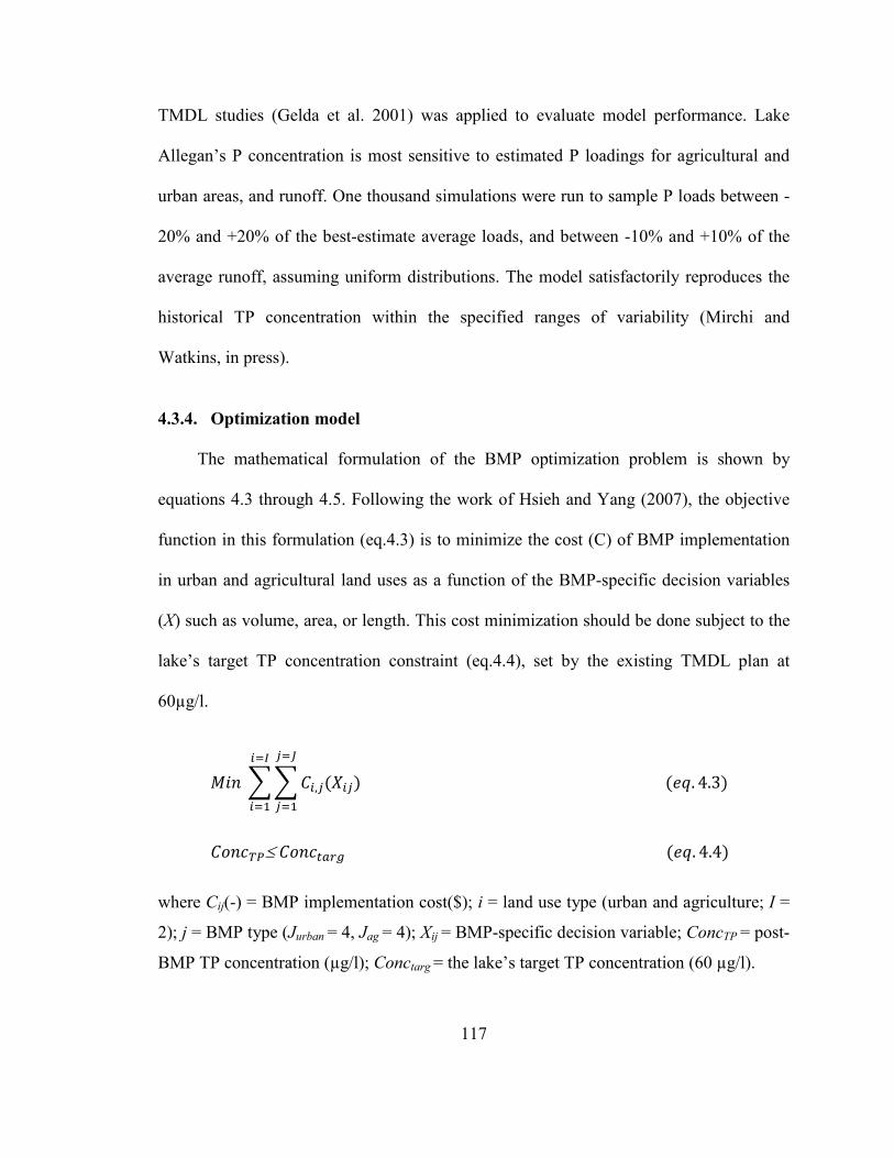
117
TMDL studies (Gelda et al. 2001) was applied to evaluate model performance. Lake
Allegan’s P concentration is most sensitive to estimated P loadings for agricultural and
urban areas, and runoff. One thousand simulations were run to sample P loads between -
20% and +20% of the best-estimate average loads, and between -10% and +10% of the
average runoff, assuming uniform distributions. The model satisfactorily reproduces the
historical TP concentration within the specified ranges of variability (Mirchi and
Watkins, in press).
4.3.4. Optimization model
The mathematical formulation of the BMP optimization problem is shown by
equations 4.3 through 4.5. Following the work of Hsieh and Yang (2007), the objective
function in this formulation (eq.4.3) is to minimize the cost (C) of BMP implementation
in urban and agricultural land uses as a function of the BMP-specific decision variables
(X) such as volume, area, or length. This cost minimization should be done subject to the
lake’s target TP concentration constraint (eq.4.4), set by the existing TMDL plan at
60µg/l.
𝑀𝑖𝑛 ��𝐶𝑖,𝑗(𝑋𝑖𝑗)𝑗=𝐽
𝑗=1
𝑖=𝐼
𝑖=1
(𝑒𝑞. 4.3)
𝐶𝑜𝑛𝑐𝑇𝑃≤ 𝐶𝑜𝑛𝑐𝑡𝑎𝑟𝑔 (𝑒𝑞. 4.4)
where Cij(-) = BMP implementation cost($); i = land use type (urban and agriculture; I =
2); j = BMP type (Jurban = 4, Jag = 4); Xij = BMP-specific decision variable; ConcTP = post-
BMP TP concentration (µg/l); Conctarg = the lake’s target TP concentration (60 µg/l).
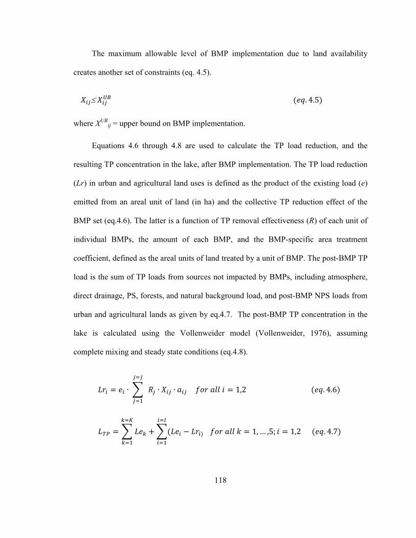
118
The maximum allowable level of BMP implementation due to land availability
creates another set of constraints (eq. 4.5).
𝑋𝑖𝑗≤ 𝑋𝑖𝑗𝑈𝐵 (𝑒𝑞. 4.5)
where XUBij = upper bound on BMP implementation.
Equations 4.6 through 4.8 are used to calculate the TP load reduction, and the
resulting TP concentration in the lake, after BMP implementation. The TP load reduction
(Lr) in urban and agricultural land uses is defined as the product of the existing load (e)
emitted from an areal unit of land (in ha) and the collective TP reduction effect of the
BMP set (eq.4.6). The latter is a function of TP removal effectiveness (R) of each unit of
individual BMPs, the amount of each BMP, and the BMP-specific area treatment
coefficient, defined as the areal units of land treated by a unit of BMP. The post-BMP TP
load is the sum of TP loads from sources not impacted by BMPs, including atmosphere,
direct drainage, PS, forests, and natural background load, and post-BMP NPS loads from
urban and agricultural lands as given by eq.4.7. The post-BMP TP concentration in the
lake is calculated using the Vollenweider model (Vollenweider, 1976), assuming
complete mixing and steady state conditions (eq.4.8).
𝐿𝑟𝑖 = 𝑒𝑖 ∙ � 𝑅𝑗 ∙ 𝑋𝑖𝑗 ∙ 𝑎𝑖𝑗
𝑗=𝐽
𝑗=1
𝑓𝑜𝑟 𝑎𝑙𝑙 𝑖 = 1,2 (𝑒𝑞. 4.6)
𝐿𝑇𝑃 = �𝐿𝑒𝑘
𝑘=𝐾
𝑘=1
+ �(𝐿𝑒𝑖 − 𝐿𝑟𝑖)
𝑖=𝐼
𝑖=1
𝑓𝑜𝑟 𝑎𝑙𝑙 𝑘 = 1, … ,5; 𝑖 = 1,2 (𝑒𝑞. 4.7)
119
𝐶𝑜𝑛𝑐𝑇𝑃 = �1
𝑄𝐿 + 𝑉𝑠𝐴𝐿� ∙ 𝐿𝑇𝑃 (𝑒𝑞. 4.8)
where Lrij = reduced load (kg/yr); ei = TP export coefficient (kg/ha/yr); Rj = removal
effectiveness coefficient (dimensionless); aij = area treatment coefficient (ha/m3, ha/m, or
ha/ha); LTP,i = post-BMP TP load (kg/yr); Lei = existing TP load (kg/yr); k = TP sources
not affected by BMPs (K = 5); QL= lake’s average discharge rate (L/yr); AL = lake’s
surface area (m2); Vs = in-lake settling velocity of TP (m/yr).
The feasible least-cost BMP set may be found using either linear programming (LP)
or a genetic algorithm (GA).
4.4. Best management practices
A suite of conventional structural and non-structural BMPs for reducing TP load
from urban and agricultural lands is considered, including basin practices (e.g., retention,
detention, and constructed wetland), grassed swales, tillage practices, and buffer strips.
Table 1 presents these BMPs, providing average cost functions, average annual operation
and maintenance cost, and average TP removal effectiveness coefficients, which have
been compiled from the literature (e.g., Bottcher et al., 1995; US EPA, 1999 and 2003;
Sample et al., 2003; Weiss et al., 2007; Simpson and Weammert, 2009; Stagge et al.,
2012). For buffer strips, a cost function was developed using the average of the cost
range from US EPA (1999), assuming a width of 10 m. Net present value of the BMP
costs was calculated for a service life of 30 years using a discount rate of 3% (eq. 4.9).
120
𝑁𝑃𝑉(𝑖,𝑇) = �𝐶𝑡
(1 + 𝑖)𝑡
𝑡=𝑇
𝑡=0
𝑓𝑜𝑟 𝑎𝑙𝑙 𝑡 = 0,1, 2, … , 30 (𝑒𝑞. 4.9)
where NPV = net present value; i = discount rate (3%); t = time (year); C = annual cost,
which includes both investment cost and annual operations and maintenance costs.
A procedure using geographic information system (GIS) and available BMP
guidelines (e.g., US EPA 1996, 2003, and 2010) was developed to identify potential
locations that are suitable for BMP implementation in order to estimate the upper bound
for BMP implementation. Up to 2% of low-lying lands with moderately and poorly
drained hydric soils, i.e., hydrologic group B, C, and D (Cronshey, 1986), in urban and
agricultural areas are considered for the storage BMPs (US EPA, 1996 and 2010). Urban
grassed swale with and without buffer strip is considered for construction along
moderately sloped (1-4%) main roads in highly developed areas with non-hydric soils of
type A and B (US EPA, 1996). Well- and moderately-well drained soils are suitable for
conservation tillage for corn production (DeJong-Hughes and Vetsch, 2007), which is the
main agricultural crop in the watershed, whereas cover cropping can be used in all
agricultural lands where conventional tillage is applied (Simpson and Weammert, 2009).
All the streams running through agricultural lands are deemed suitable for
implementation of agricultural buffer strips. These siting criteria are summarized in
Table 4.2. Urban and agricultural TP load export coefficients and BMP-specific attributes
such as upper bound and area treatment coefficients are provided in Table 4.3.
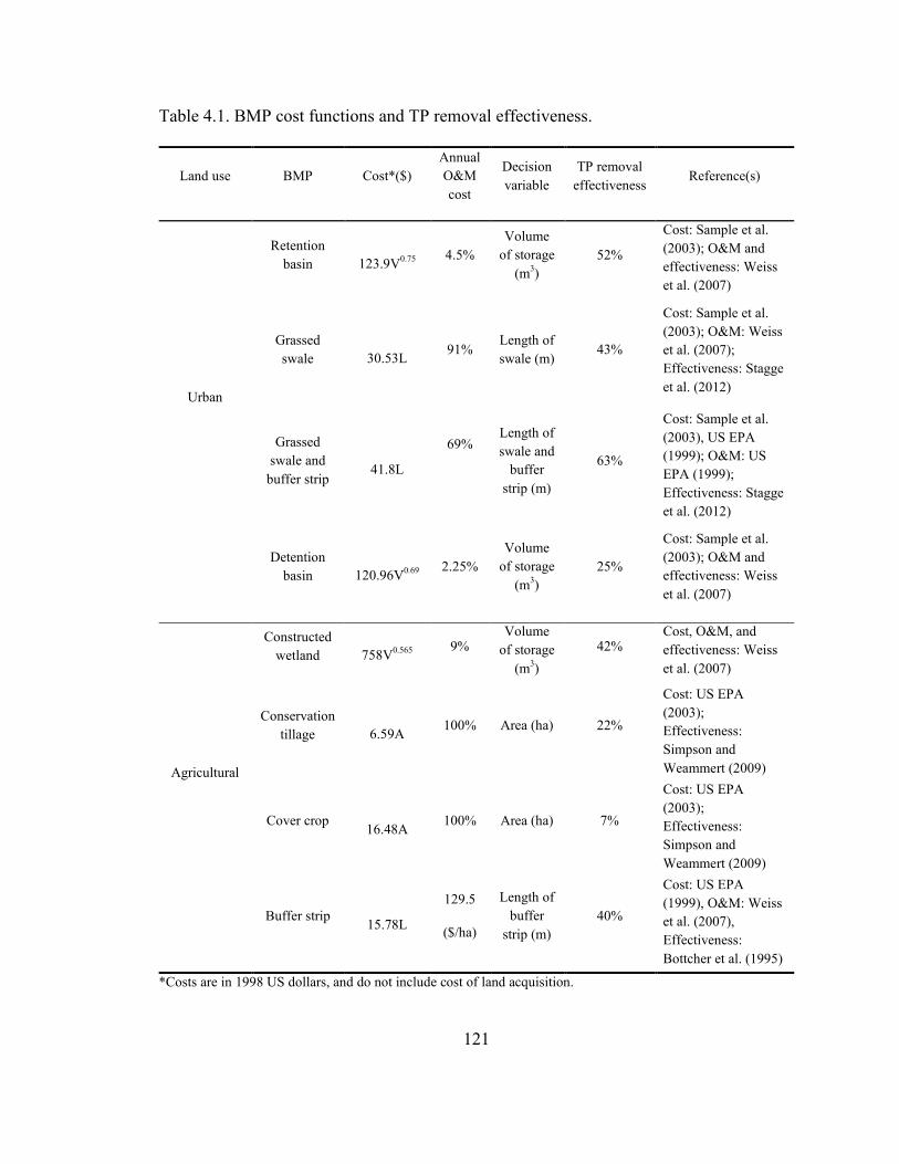
121
Table 4.1. BMP cost functions and TP removal effectiveness.
Land use BMP Cost*($) Annual O&M cost
Decision variable
TP removal effectiveness
Reference(s)
Urban
Retention basin 123.9V0.75 4.5%
Volume of storage
(m3) 52%
Cost: Sample et al. (2003); O&M and effectiveness: Weiss et al. (2007)
Grassed swale 30.53L 91%
Length of swale (m)
43%
Cost: Sample et al. (2003); O&M: Weiss et al. (2007); Effectiveness: Stagge et al. (2012)
Grassed swale and
buffer strip 41.8L
69%
Length of swale and
buffer strip (m)
63%
Cost: Sample et al. (2003), US EPA (1999); O&M: US EPA (1999); Effectiveness: Stagge et al. (2012)
Detention basin 120.96V0.69 2.25%
Volume of storage
(m3) 25%
Cost: Sample et al. (2003); O&M and effectiveness: Weiss et al. (2007)
Agricultural
Constructed wetland 758V0.565 9%
Volume of storage
(m3) 42%
Cost, O&M, and effectiveness: Weiss et al. (2007)
Conservation tillage 6.59A 100% Area (ha) 22%
Cost: US EPA (2003); Effectiveness: Simpson and Weammert (2009)
Cover crop 16.48A 100% Area (ha) 7%
Cost: US EPA (2003); Effectiveness: Simpson and Weammert (2009)
Buffer strip 15.78L
129.5
($/ha)
Length of buffer
strip (m) 40%
Cost: US EPA (1999), O&M: Weiss et al. (2007), Effectiveness: Bottcher et al. (1995)
*Costs are in 1998 US dollars, and do not include cost of land acquisition.
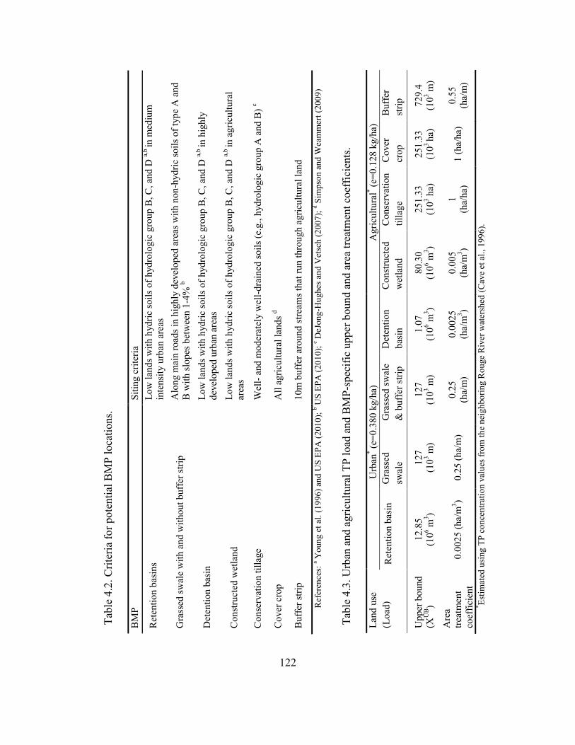
122
Tabl
e 4.
2. C
riter
ia fo
r pot
entia
l BM
P lo
catio
ns.
BM
P Si
ting
crite
ria
Ret
entio
n ba
sins
Lo
w la
nds w
ith h
ydric
soils
of h
ydro
logi
c gr
oup
B, C
, and
D a,
b in
med
ium
in
tens
ity u
rban
are
as
Gra
ssed
swal
e w
ith a
nd w
ithou
t buf
fer s
trip
Alo
ng m
ain
road
s in
high
ly d
evel
oped
are
as w
ith n
on-h
ydric
soils
of t
ype
A a
nd
B w
ith sl
opes
bet
wee
n 1-
4% b
Det
entio
n ba
sin
Low
land
s with
hyd
ric so
ils o
f hyd
rolo
gic
grou
p B
, C, a
nd D
a,b in
hig
hly
deve
lope
d ur
ban
area
s
Con
stru
cted
wet
land
Lo
w la
nds w
ith h
ydric
soils
of h
ydro
logi
c gr
oup
B, C
, and
D a,
b in
agr
icul
tura
l ar
eas
Con
serv
atio
n til
lage
W
ell-
and
mod
erat
ely
wel
l-dra
ined
soils
(e.g
., hy
drol
ogic
gro
up A
and
B) c
Cov
er c
rop
All
agric
ultu
ral l
ands
d
Buf
fer s
trip
10m
buf
fer a
roun
d st
ream
s tha
t run
thro
ugh
agric
ultu
ral l
and
Ref
eren
ces:
a You
ng e
t al.
(199
6) a
nd U
S EP
A (2
010)
; b US
EPA
(201
0); c D
eJon
g-H
ughe
s and
Vet
sch
(200
7); d S
imps
on a
nd W
eam
mer
t (20
09)
Tabl
e 4.
3. U
rban
and
agr
icul
tura
l TP
load
and
BM
P-sp
ecifi
c up
per b
ound
and
are
a tre
atm
ent c
oeff
icie
nts.
Land
use
(L
oad)
Urb
an* (e
=0.3
80 k
g/ha
) A
gric
ultu
ral* (e
=0.1
28 k
g/ha
) R
eten
tion
basi
n G
rass
ed
swal
e G
rass
ed sw
ale
& b
uffe
r stri
p D
eten
tion
basi
n C
onst
ruct
ed
wet
land
C
onse
rvat
ion
tilla
ge
Cov
er
crop
B
uffe
r st
rip
Upp
er b
ound
(X
UB )
12.8
5 (1
06 m3 )
127
(1
03 m)
127
(103 m
) 1.
07
(106 m
3 ) 80
.30
(106 m
3 ) 25
1.33
(1
03 ha)
25
1.33
(1
03 ha
) 72
9.4
(103 m
)
Are
a tre
atm
ent
coef
ficie
nt
0.00
25 (h
a/m
3 ) 0.
25 (h
a/m
) 0.
25
(ha/
m)
0.00
25
(ha/
m3 )
0.00
5 (h
a/m
3 ) 1
(ha/
ha)
1 (h
a/ha
) 0.
55
(ha/
m)
* Estim
ated
usi
ng T
P co
ncen
tratio
n va
lues
from
the
neig
hbor
ing
Rou
ge R
iver
wat
ersh
ed (C
ave
et a
l., 1
996)
.
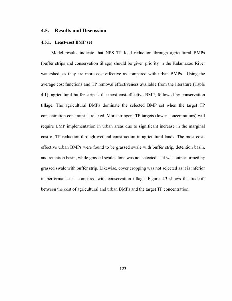
123
4.5. Results and Discussion
4.5.1. Least-cost BMP set
Model results indicate that NPS TP load reduction through agricultural BMPs
(buffer strips and conservation tillage) should be given priority in the Kalamazoo River
watershed, as they are more cost-effective as compared with urban BMPs. Using the
average cost functions and TP removal effectiveness available from the literature (Table
4.1), agricultural buffer strip is the most cost-effective BMP, followed by conservation
tillage. The agricultural BMPs dominate the selected BMP set when the target TP
concentration constraint is relaxed. More stringent TP targets (lower concentrations) will
require BMP implementation in urban areas due to significant increase in the marginal
cost of TP reduction through wetland construction in agricultural lands. The most cost-
effective urban BMPs were found to be grassed swale with buffer strip, detention basin,
and retention basin, while grassed swale alone was not selected as it was outperformed by
grassed swale with buffer strip. Likewise, cover cropping was not selected as it is inferior
in performance as compared with conservation tillage. Figure 4.3 shows the tradeoff
between the cost of agricultural and urban BMPs and the target TP concentration.
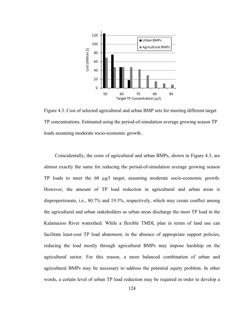
124
Figure 4.3. Cost of selected agricultural and urban BMP sets for meeting different target
TP concentrations. Estimated using the period-of-simulation average growing season TP
loads assuming moderate socio-economic growth.
Coincidentally, the costs of agricultural and urban BMPs, shown in Figure 4.3, are
almost exactly the same for reducing the period-of-simulation average growing season
TP loads to meet the 60 µg/l target, assuming moderate socio-economic growth.
However, the amount of TP load reduction in agricultural and urban areas is
disproportionate, i.e., 80.7% and 19.3%, respectively, which may create conflict among
the agricultural and urban stakeholders as urban areas discharge the most TP load in the
Kalamazoo River watershed. While a flexible TMDL plan in terms of land use can
facilitate least-cost TP load abatement, in the absence of appropriate support policies,
reducing the load mostly through agricultural BMPs may impose hardship on the
agricultural sector. For this reason, a more balanced combination of urban and
agricultural BMPs may be necessary to address the potential equity problem. In other
words, a certain level of urban TP load reduction may be required in order to develop a
125
fairer TMDL plan, although this may cause divergence from the least-cost BMP set.
Figure 4.4 illustrates how the BMP implementation at the watershed scale becomes
suboptimal under different scenarios of urban TP load reduction as compared with a
flexible TMDL plan where the required urban TP load reduction is 0%. The figure
indicates that there is potential for policies that allow for optimal abatement of TP loads
at the watershed scale through environmental offset programs between urban and
agricultural areas, whereby urban areas share the cost of agricultural BMP
implementation.
Figure 4.4. Tradeoff contours for different urban load reduction requirements.
4.5.2. Effect of socioeconomic growth
If the reported land use-based TP export coefficients (urban: 0.380 kg/ha,
agricultural: 0.128 kg/ha) for the Kalamazoo River watershed hold into the future, it can
be expected that TP load to the lake will increase over time as a consequence of
126
urbanization driven by socioeconomic growth (Mirchi and Watkins, in press). Four
socioeconomic growth scenarios were considered in this study based on historical trends
of population growth, employment, and income. These scenarios are static conditions,
slow growth, moderate growth, and rapid growth, which are equivalent to annual
population growth rates of 0%, 0.1%, 0.56%, and 1%, respectively. Figure 4.5 shows the
TP concentration exceedence curves for static conditions, along with moderate and rapid
economic growth scenarios for the two cases of without and with BMPs. The
concentration exceedence curves illustrate the effect of the least-cost BMP set obtained
using period-of-simulation average growing season TP loads. The BMPs increase
nutrient assimilation capacity of the area, which supports economic growth while
maintaining the violation of the water quality goal at a minimal level. The probability of
exceedence of the target concentration (60 µg/l) is reduced from ~40% when BMPs are
not implemented to ~20% after BMP implementation. Table 4.4 summarizes the required
TP load reduction and reliability of the least-cost BMP set for meeting the concentration
target under different economic growth and BMP implementation scenarios.
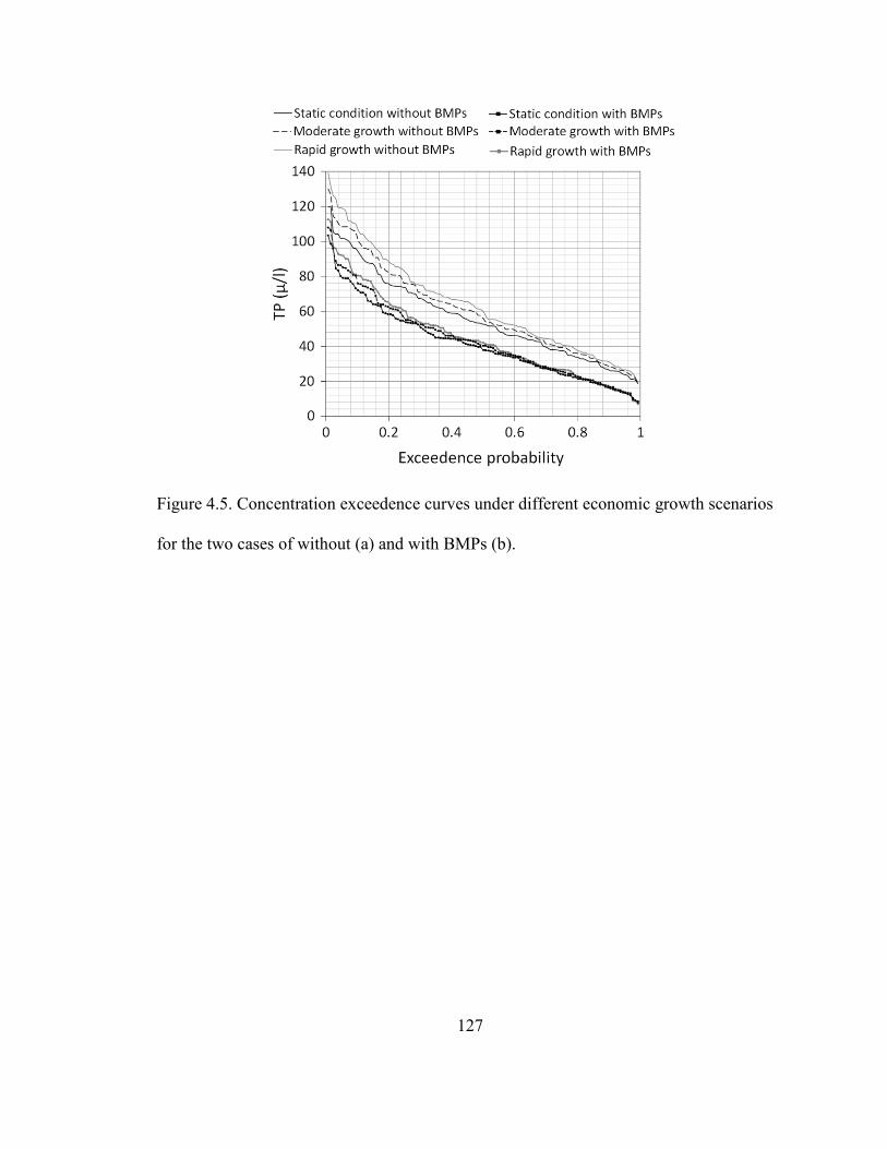
127
Figure 4.5. Concentration exceedence curves under different economic growth scenarios
for the two cases of without (a) and with BMPs (b).
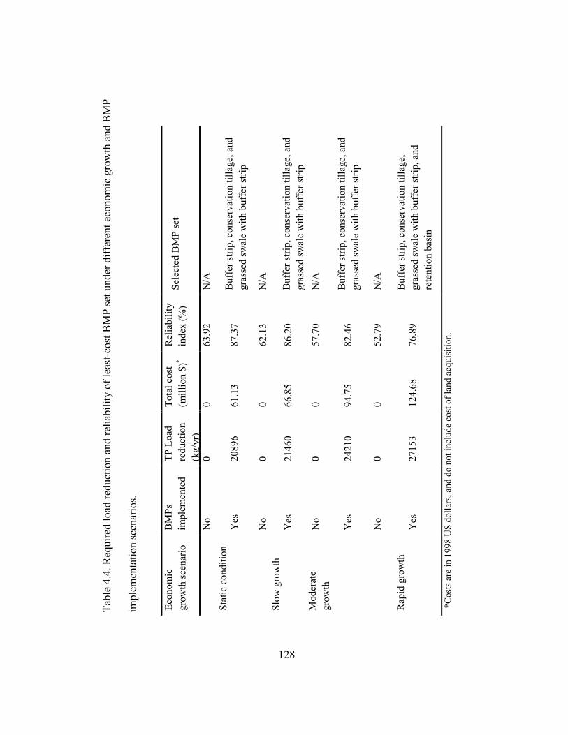
128
Tabl
e 4.
4. R
equi
red
load
redu
ctio
n an
d re
liabi
lity
of le
ast-c
ost B
MP
set u
nder
diff
eren
t eco
nom
ic g
row
th a
nd B
MP
impl
emen
tatio
n sc
enar
ios.
*Cos
ts a
re in
199
8 U
S do
llars
, and
do
not i
nclu
de c
ost o
f lan
d ac
quis
ition
.
Econ
omic
gr
owth
scen
ario
B
MPs
im
plem
ente
d TP
Loa
d re
duct
ion
(kg/
yr)
Tota
l cos
t (m
illio
n $)
* R
elia
bilit
y in
dex
(%)
Sele
cted
BM
P se
t
Stat
ic c
ondi
tion
No
0 0
63.9
2 N
/A
Yes
20
896
61.1
3 87
.37
Buf
fer s
trip,
con
serv
atio
n til
lage
, and
gr
asse
d sw
ale
with
buf
fer s
trip
Slow
gro
wth
N
o 0
0 62
.13
N/A
Yes
21
460
66.8
5 86
.20
Buf
fer s
trip,
con
serv
atio
n til
lage
, and
gr
asse
d sw
ale
with
buf
fer s
trip
Mod
erat
e gr
owth
N
o 0
0 57
.70
N/A
Y
es
2421
0 94
.75
82.4
6 B
uffe
r stri
p, c
onse
rvat
ion
tilla
ge, a
nd
gras
sed
swal
e w
ith b
uffe
r stri
p
Rap
id g
row
th
No
0 0
52.7
9 N
/A
Yes
27
153
124.
68
76.8
9 B
uffe
r stri
p, c
onse
rvat
ion
tilla
ge,
gras
sed
swal
e w
ith b
uffe
r stri
p, a
nd
rete
ntio
n ba
sin
129
4.5.3. Uncertainty in TMDL planning
There is a multitude of sources of uncertainty that complicate the TMDL planning
for NPS pollutant abatement, including imperfect information, natural variability, and
knowledge-based inconsistency (Shirmohammadi et al., 2006; Chen et al., 2007; Keller
and Cavallaro, 2008). Uncertainty is inherent in the process of identifying the sources and
magnitude of NPS pollution due to paucity of field data because of infrequent and limited
monitoring campaigns, and inconsistent assessment methods (Keller and Cavallaro,
2008). There is significant uncertainty about the BMPs’ pollutant removal effectiveness
due to lack of a systematic approach for data collection and comparative assessment of
stormwater pollutant removal (Strecker et al., 2001; Scholes et al., 2008), as well as site-
to-site variability. Furthermore, determining the reference hydrologic conditions for
developing the TMDL to adequately capture natural variability is a major source of
uncertainty. Consequently, TMDL planners are faced with a wide range of potential
strategies (e.g., combination of BMPs) for addressing the NPS pollution, which bears
significant cost implications.
To illustrate the potential effect of uncertainties on the projected trend of TP
concentration, a Monte Carlo analysis was performed using two thousand simulations
between static and rapid growth conditions. Furthermore, +/- 10% variability in runoff
was considered, and TP loads were sampled from a uniform distribution between -20%
and +20% of the best-estimate average loads. The results of these simulations are shown
in Figure 4.6 for the two cases of without and with BMPs. The figure illustrates that
meeting the Lake Allegan’s TP concentration target in any given year is primarily
governed by intra- and inter-annual hydrologic variability, making the impacts of
130
socioeconomic growth secondary in importance. In this situation, the lake’s hydraulic
flushing during the growing season is a significant determinant of eutrophication because
the amount of TP in the Kalamazoo River is generally high (Reid and Hamilton, 2007).
Therefore, NPS TP loads may have to be greatly reduced before the lake’s water quality
target can be met with high reliability. Furthermore, the long-term attainability of the
target TP concentration may be contingent on updating of the NPS load reduction
requirement to account for the effect of economically-driven urbanization.
The tradeoffs between TP load abatement cost and the reliability of attaining the
water quality target are substantial. To illustrate this effect, the BMP optimization model
was run under stochastic hydrologic (and resulting TP load) conditions using the Monte
Carlo technique, assuming moderate socioeconomic growth. The least-cost BMP set from
the optimization model with mean TP load estimates was used as a good initial guess in
order to increase computational efficiency. Two thousand random samples of TP load
were taken for different NPSs from a uniform distribution within two standard deviations
of the average growing season TP load. The outcome of this process is two thousand
least-cost BMP sets corresponding to different load conditions. Figure 4.7 shows the cost
implication of this uncertainty due to TP load variability associated with inter-annual
hydrologic variability. The long right-tail of the histogram denotes greater TP load
reduction through more extensive BMP implementation using basin BMPs, providing a
higher reliability but at significantly higher costs as compared with the average condition
(~$95 million).
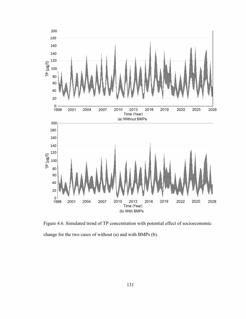
131
Figure 4.6. Simulated trend of TP concentration with potential effect of socioeconomic
change for the two cases of without (a) and with BMPs (b).
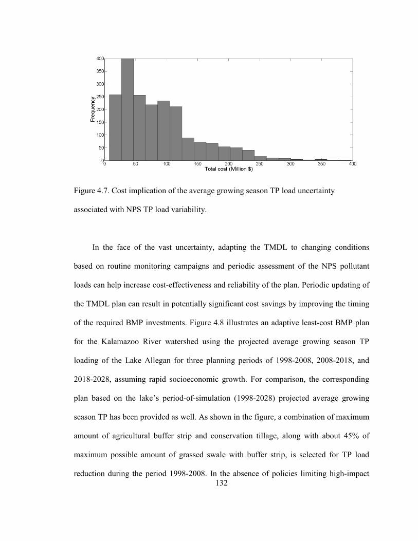
132
Figure 4.7. Cost implication of the average growing season TP load uncertainty
associated with NPS TP load variability.
In the face of the vast uncertainty, adapting the TMDL to changing conditions
based on routine monitoring campaigns and periodic assessment of the NPS pollutant
loads can help increase cost-effectiveness and reliability of the plan. Periodic updating of
the TMDL plan can result in potentially significant cost savings by improving the timing
of the required BMP investments. Figure 4.8 illustrates an adaptive least-cost BMP plan
for the Kalamazoo River watershed using the projected average growing season TP
loading of the Lake Allegan for three planning periods of 1998-2008, 2008-2018, and
2018-2028, assuming rapid socioeconomic growth. For comparison, the corresponding
plan based on the lake’s period-of-simulation (1998-2028) projected average growing
season TP has been provided as well. As shown in the figure, a combination of maximum
amount of agricultural buffer strip and conservation tillage, along with about 45% of
maximum possible amount of grassed swale with buffer strip, is selected for TP load
reduction during the period 1998-2008. In the absence of policies limiting high-impact
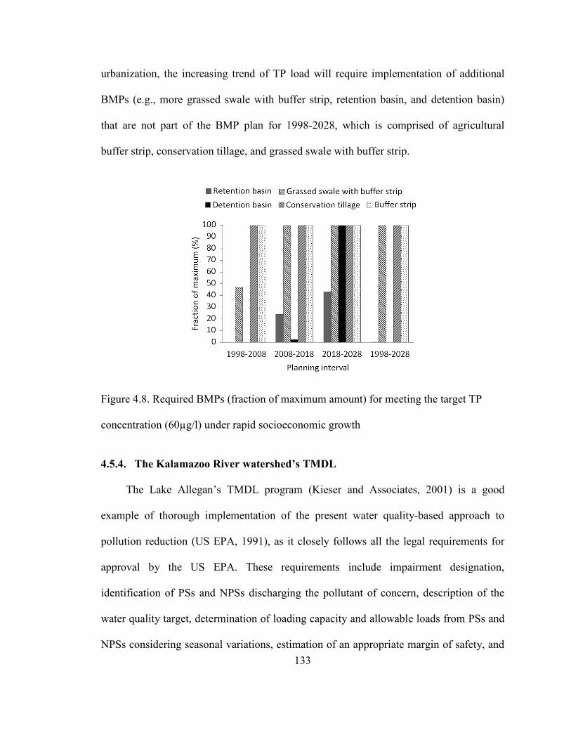
133
urbanization, the increasing trend of TP load will require implementation of additional
BMPs (e.g., more grassed swale with buffer strip, retention basin, and detention basin)
that are not part of the BMP plan for 1998-2028, which is comprised of agricultural
buffer strip, conservation tillage, and grassed swale with buffer strip.
Figure 4.8. Required BMPs (fraction of maximum amount) for meeting the target TP
concentration (60µg/l) under rapid socioeconomic growth
4.5.4. The Kalamazoo River watershed’s TMDL
The Lake Allegan’s TMDL program (Kieser and Associates, 2001) is a good
example of thorough implementation of the present water quality-based approach to
pollution reduction (US EPA, 1991), as it closely follows all the legal requirements for
approval by the US EPA. These requirements include impairment designation,
identification of PSs and NPSs discharging the pollutant of concern, description of the
water quality target, determination of loading capacity and allowable loads from PSs and
NPSs considering seasonal variations, estimation of an appropriate margin of safety, and
134
adequate monitoring (US EPA, 1991). Although not a requirement for approval, TMDL
planners are also strongly encouraged to provide an implementation plan with reasonable
assurances for NPS load reduction on a voluntary basis (US EPA, 1991). The TMDL
development process for Lake Allegan was completed through close stakeholder
involvement within a participatory framework, facilitating a “cooperative agreement”
between PS and NPS polluters whereby PSs (e.g., wastewater and industrial dischargers)
assist NPSs (e.g., farmers) to reduce TP loads (KRLATIC, 2002).
Clearly, the voluntary NPS TP reduction in the Kalamazoo River watershed has not
been on par with that of PS reductions (Kieser and Associates, 2011), which may be part
of the reason why the lake’s recovery appears to be slower than anticipated. There is a
growing need for more aggressive NPS TP load reduction policies because of the
significant increase in the marginal cost of additional PS abatement. However, the
command and control approaches to environmental management are particularly difficult
to apply to “wicked” problems such as NPS pollution due to potentially substantial
socioeconomic implications. Centner et al. (1999) investigated the challenges of BMP
implementation from a legal institution perspective, and concluded that NPS pollution
abatement may be prohibitively costly to agricultural producers, indicating that
government intervention will be necessary for nutrient load reduction. The results of the
developed BMP optimization model of the Kalamazoo River watershed corroborate this
notion. Using average growing season TP loads and assuming a moderate socioeconomic
growth scenario, the implementation cost of agricultural BMPs, excluding the cost of
land acquisition and opportunity cost of land, is ~$50 million, providing a reliability
index of slightly greater than 80%. Model results indicate that more stringent NPS TP
135
reduction with significantly higher costs would be necessary for achieving higher
reliability.
The presented simulation-optimization framework can facilitate application of
systems thinking and environmental systems analysis techniques to the Lake Allegan
TMDL program. The costs associated with BMP implementation should be viewed as a
necessary environmental investment in order to maintain beneficial uses of the lake,
avoiding the negative impact of environmental deterioration on socioeconomic growth. A potential area of improvement for the current TMDL program is projection of future
socioeconomic growth and its potential implications for attainability of the water quality
target. Furthermore, while the Lake Allegan’s TMDL implementation plan has
recognized the importance of identifying cost-effective abatement strategies and funding
policies, systematic methods have not been applied. The full financial burden of BMP
implementation may threaten to slow down the local socioeconomic growth. Systematic
BMP optimization using sufficient site-specific water quality and BMP performance
information can facilitate securing of adequate external funds through federal and state
sources (e.g., cost shares for agricultural BMPs), which can balance the negative impact
on the area’s socioeconomic growth (e.g., US EPA, 2003).
136
4.5.5. Limitations
Simplifications are inherent in any modeling effort (Box and Draper, 1987), causing
models to be different from reality in infinitely many ways (Sterman, 2000). In addition
to the significant uncertainties involved in the TMDL studies, the limitations of the
presented quantitative-qualitative methodology for finding least-cost BMPs need to be
recognized in order to provide realistic insights for TMDL policy. The Lake Allegan SD
model is a high-level simulation tool. Significantly more socioeconomic and biophysical
details could be used for representing different feedback loops subject to data availability
and the desired level of sophistication for characterizing the system-wide processes
driving the degradation of aquatic systems. Socioeconomic growth, land use change over
time, and hydrologic conditions have been simulated in a lumped fashion at the
watershed-scale, and potential changes in climatic conditions have not been considered.
Some of the links in the integrated SD simulation models are difficult to quantify, e.g.,
the negative link between environmental degradation and socioeconomic growth, which
creates a balancing biophysical feedback loop.
Another limitation is the use of literature-reported cost functions and the BMP-
specific TP removal effectiveness coefficients in the optimization model. Wide ranges of
variability have been reported in the literature for TP removal effectiveness coefficient of
different BMPs (e.g., Bottcher et al., 1995). The uncertainty associated with lack of
information about the actual performance of different BMPs can influence the choice of
the least-cost BMP set, affecting the reliability of meeting the target. Site-specific
analyses should be conducted for actual BMP implementation, accounting for the local
137
variability of BMP implementation cost, cost of land acquisition, and opportunity cost of
land.
Despite the existing limitations, the methodology facilitates investigation of the
tradeoffs between BMP implementation cost and attainable water quality targets. The use
of GA allows for exploration of a wide range of possible BMP sets with non-linear cost-
functions that capture economies of scale, whereas linear watershed scale cost functions
should be used when applying a LP model. Stochastic elements can be incorporated in
the optimization framework using site-specific ranges to characterize TMDL uncertainty
and associated cost implications, although stochastic optimization using GA is
computationally intensive. The screening level optimization model provides insights to
least-cost BMPs and the cost of NPS TP load reduction, guiding cooperative agreements
between individual PS and NPS polluters, as well as more extensive environmental offset
programs facilitating TMDL implementation. Projection of the long-term adequacy of the
proposed load reductions and potential impacts of socioeconomic growth on attainment
of the target helps strategize BMP implementation policies.
4.6. Conclusions
The simulation-optimization framework presented herein facilitates application of
systems thinking and environmental systems analysis to TMDL programs. A screening-
level deterministic optimization model was used in conjunction with a system dynamics
simulation model to investigate TP load reduction in the Kalamazoo River watershed.
The results suggest that there is significant potential for cost-effective TP load abatement
mostly through agricultural BMPs, as policies requiring substantial (>20%) urban TP
138
load reduction are sub-optimal compared with greater abatement of agricultural loads.
However, without sufficient support policies, the NPS pollution abatement required for
achieving the Lake Allegan’s TP concentration target with high reliability can be
prohibitively costly to agricultural producers, indicating the need for government
intervention, as well as potential for environmental offset programs between urban and
agricultural areas. Furthermore, while the lake’s TP concentration is primarily governed
by intra- and inter-annual hydrologic variability, the socioeconomic growth of the
watershed negatively affects the reliability of meeting the water quality goal, if the target
were to be achieved using TMDLs designated assuming static conditions.
Implementation of TMDLs as required by the US CWA is a good opportunity for
application of a long-term systems approach for reducing NPS pollution. Based on the
US EPA guidelines for a water quality-based approach to pollution abatement, the
Kalamazoo River watershed’s TMDL program has been a successful initiative. PS
polluters have been reasonably successful in reducing TP emissions. However, in spite of
a collective watershed-scale effort using a participatory and cooperative framework, the
voluntary NPS TP load abatement has only been partially successful, possibly delaying
the attainment of the water quality goal. More aggressive TMDL implementation policies
are needed to address the NPS TP emissions. The Lake Allegan program can be
improved by accounting for future socioeconomic growth trends and its potential
implications for attainability of the water quality target. Furthermore, the program should
be equipped with environmental systems analysis methods in order to identify cost-
effective abatement strategies, as well as equitable funding policies.
139
4.7. References
Arabi, M., Govindaraju, R. S., Hantush, M. M. (2006). Costeffective allocation of
watershed management practices using a genetic algorithm. Water Resources
Research 42, W10429.
Booth, D.B., Jackson, C.R. (1997). Urbanization of aquatic systems: degradation
thresholds, stormwater detection, and the limits of mitigation. Journal of
American Water Resources Association 33, 311–23.
Bottcher, A.B., Tremwell, T., Campbell, K.L. (1995). Best management practices for
water quality improvement in the Lake Okeechobee watershed. Ecological
Engineering 5, 341-356.
Boyd, J. (2000). The new faces of the Clean Water Act: A critical review of the EPA’s
proposed TMDL rules (discussion paper 00-12). Resources for the Future,
Washington, DC.
Box, G.E.P., Draper, N.R. (1987). Empirical Model-building and Response Surfaces.
John Wiley, New York.
Carpenter, S.R., Caraco, N.F., Correll, D.L., Howarth, R.W., Sharpley, A.N., Smith, V.H.
(1998). Nonpoint pollution of surface waters with phosphorus and nitrogen.
Ecological Applications 8, 559–68.
Cave, K., Harold, E., Quasebarth, T. (1996). Preliminary pollution loading projections for
Rouge River watershed and interim nonpoint source pollution control plan,
Technical Report RPO-NPS-TR07.00, Rouge River National Wet Weather
Demonstration Project, Wayne County, Michigan.
140
Centner, T.J. , Houston, J.E., Keeler, A.G., Fuchs, C. (1999). The Adoption of Best
Management Practices to Reduce Agricultural Water Contamination Limnologica
29, 366–373.
Chen, C.F., Ma, H.W., Reckhow, K.H. (2007). Assessment of water quality management
with a systematic qualitative uncertainty analysis. Science of the Total
Environment 374 (1), 13–25.
Correll, D.L. (1998). The role of phosphorus in the eutrophication of receiving waters: a
review. Journal of Environmental Quality 27, 261-266.
DeJong-Hughes, J. and Vetsch, J. (2007). On-farm comparison of conservation tillage
systems for corn following soybeans. University of Minnesota Extension Bulletin
08483.
Deng, X., Zhao, Y., Wu, F., Lin, Y., Lu, Q., Dai, J. (2011). Analysis of the trade-off
between economic growth and the reduction of nitrogen and phosphorus
emissions in the Poyang Lake Watershed, China. Ecological Modeling 222, 330–
336.
Forrester, J. (1961) Industrial dynamics. MIT Press, Cambridge.
Forrester, J. (1969) Urban dynamics. MIT Press, Cambridge.
FWPCA (1972). Federal water pollution control act, as amended (33 U.S.C. 1151 et
seq.).
FWPCA (2002). Federal water pollution control act, as amended (33 U.S.C. 1251 et
seq.).
141
Gburek, W.J., Sharpley, A.N., Heathwaite, L., Folmar, G.J. (2000). Phosphorus
management at the watershed scale: A modification of the phosphorus index.
Journal of Environmental Quality 29, 130–144.
Gelda, R. K., Effler, S. W., O’Donnell, S. M. (2001). Probabilistic model of ammonia
and toxicity status for urban lake. Journal of Water Resources Planning
Management 127(5), 337–347.
Giri, S., Nejadhashemi, A.P., Woznicki, S.A. (2012). Evaluation of targeting methods for
implementation of best management practices in the Saginaw River Watershed.
Journal of Environmental Management 103, 24-40.
Gitau, M.W., Veith, T.L., Gburek, W.J. (2004). Farm-level optimization of BMP
placement for cost-effective pollution reduction. Transaction of The American
Society of Agricultural and Biological Engineers 47 (6), 1923–1931.
Gooday, R. D., Anthony, S. G., Chadwick, D. R., Newell-Price, P., Harris, D.,
Duethmann, D., Fish, R., Collins, A. L., Winter, M. (in press). Modelling the cost-
effectiveness of mitigation methods for multiple pollutants at farm scale. Science
of The Total Environment, doi: 10.1016/j.scitotenv.2013.04.078.
Haygarth, P. M., Condron, L. M., Heathwaite, A. L., Turner, B. L., Harris, G. P. (2005).
The phosphorous transfer continuum: linking source to impact with an
interdisciplinary and multiscaled approach. Science of the Total Environment 344,
5-14.
Heaton, S. (2001). Total maximum daily load (TMDL) for total phosphorus in Lake
Allegan. Surface Water Quality Division, Michigan Department of Environmental
Quality. Lansing, Michigan.
142
Heathwaite, A.L., Quinn, P.F., Hewett, C.J.M. (2005). Modelling and managing critical
source areas of diffuse pollution from agricultural land by simulating hillslope
flow connectivity. Journal of Hydrology 304(1– 4), 446– 61.
Hein, L.G. (2006). Cost-efficient eutrophication control in a shallow lake ecosystem
subject to two steady states. Ecological Economics 59 (4), 429–439.
Hsieh, C.D., Yang, W.F. (2007). Optimal nonpoint source pollution control strategies for
a reservoir watershed in Taiwan. Journal of Environmental Management 85, 908–
917.
Keller, A. A., Cavallaro, L. (2008). Assessing the US Clean Water Act 303(d) listing
process for determining impairment of a waterbody. Journal of Environmental
Management 86, 699–711.
Kieser and Associates (2001). Non-point source modeling of phosphorus loads in the
Kalamazoo River/Lake Allegan watershed for a total maximum daily load. Kieser
and Associates Environmental Science and Engineering, Kalamazoo, Michigan.
Kieser and Associates (2011). Summary of 2010 total phosphorus loading to the
Kalamazoo River and Lake Allegan with comparisons to historic data. Kieser and
Associates Environmental Science and Engineering, (http://kalamazooriver.net/)
(Oct. 3, 2011).
Kleinman, P.J.A., Sharpley, A.N., McDowell, R.W., Flaten, D.N., Buda, A.R., Tao, L.,
Bergstrom, L., Zhu, Q. (2011). Managing agricultural phosphorus for water
quality protection: principles for progress. Plant and Soil 349,169-182.
Kalamazoo River/Lake Allegan TMDL Implementation Committee (KRLATIC) (2002).
Water quality improvement (implementation) plan for the Kalamazoo River
143
watershed and Lake Allegan through a phosphorus total maximum daily load
(TMDL) process, The Kalamazoo River/Lake Allegan TMDL Implementation
Committee, Kalamazoo, MI.
Lee, G. F., Rast, W., Jones, R. A. (1978). Eutrophication of water bodies: insights for an
age-old problem. Environmental Science and Technology 12, 900–908.
Lee, G.J., Selvakumar, A., Alvi, K., Riverson, J., Zhen, X.J., Shoemaker, L., Lai, F.
(2012). A watershed-scale design optimization model for stormwater best
management practices. Environmental Modelling & Software 37, 6-18.
Mainstone, C.P., Parr, W. (2002). Phosphorus in rivers — ecology and management.
Science of the Total Environment 282–283, 25–47.
Maringanti, C., Chaubey, I., Popp, J. (2009). Development of a multiobjective
optimization tool for the selection and placement of best management practices
for nonpoint source pollution control. Water Resources Research 45 (6), W06406.
Meadows, D.H., Meadows, D.L., Randers, J., Behrens, W.W. (1972). The limits to
growth. Universe Books, New York.
MDNR (1987). Remedial action plan for the Kalamazoo River. Michigan Department of
Natural Resources, Bay City, Michigan.
Michalak, A.M., et al. (2013). Record-setting algal bloom in Lake Erie caused by
agricultural and meteorological trends consistent with expected future conditions.
Proceedings of the National Academy of Sciences of the United States of America
110(16), 6448-6452.
Milon, J.W. (1987). Optimising NPS controls in water quality regulation. Journal of the
American Water Resources Association (3), 387–396.
144
Mirchi, A., Madani, K., Watkins D, Ahmad, S. (2012). Synthesis of system dynamics
tools for holistic conceptualization of water resources problems. Water Resources
Management 26(9), 2421-2442.
Mirchi, A., Watkins, D.W. Jr. (in press). A systems approach to holistic TMDL policy:
Case of Lake Allegan, Michigan. Journal of Water Resources Planning and
Management, doi: 10.1061/(ASCE)WR.1943-5452.0000292.
Paerl, H.W., Hall, N.S., Calandrino, E.S. (2011). Controlling harmful cyanobacterial
blooms in a world experiencing anthropogenic and climatic-induced change.
Science of the Total Environment 40, 1739-1745.
Panagopoulos, Y., Makropoulos, C., Mimikou, M. (2011). Diffuse surface water
pollution: driving factors for different geoclimatic regions. Water Resources
Management 25 (14), 3635-3660.
Panagopoulos, Y., Makropoulos, C., Mimikou, M. (2012). Decision support for diffuse
pollution management. Environmental Modelling & Software 30, 57-70.
Pijanowski, B.C., Brown, D.G., Shellito, B.A., Manik, G.A. (2002). Using neural
networks and GIS to forecast land use changes: a land transformation model.
Computers. Environment and Urban Systems 26 (6), 553–575.
Rao, N.S., Easton, Z.M., Schneiderman, E.M., Zion, M.S., Lee, D.R., Steenhuis, T.S.
(2009). Modeling Watershed-scale effectiveness of agricultural best management
practices to reduce phosphorus loading. Journal of Environmental Management
90, 1385–1395.
145
Reid, N.J., Hamilton, S.K. (2007). Controls on algal abundance in a eutrophic river with
varying degrees of impoundment (Kalamazoo River, Michigan, USA). Lake and
Reservoir Management 23, 219–230.
Rodriguez, H.G., Popp, J., Maringanti, C., Chaubey, I. (2011). Selection and placement
of best management practices used to reduce water quality degradation in Lincoln
Lake watershed. Water Resources Research 47, 1-13.
Sample, D.J., Heaney, J.P., Wright, L.T., Fan, C.Y., Lai, F.H., Field, R. (2003). Cost of
best management practices and associated land for urban stormwater control.
Journal of Water Resources Planning and Management 129(1), 59-68.
Scholes, L., Revitt, D.M., Ellis, J.B. (2008). A systematic approach for the comparative
assessment of stormwater pollutant removal potentials. Journal of Environmental
Management 88(3), 467-478.
Schwartz, S. S. (2010). Optimization and decision heuristics for Chesapeake Bay nutrient
reduction strategies. Environmental Modeling and Assessment 15(5), 345–359.
Senge, P. (1990). The fifth discipline: the art & practice of the learning organization.
Doubleday/Currency, New York.
Sharpley, A.N. (1994). Managing agricultural phosphorus for protection of surface
waters: Issues and options. Journal of Environmental Quality 23, 437–451.
Shirmohammadi, A., Chaubey, I., Harmel, R.D., Bosch, D.D., Muñoz-Carpena, R.,
Dharmasri, C., Sexton, A., Arabi, M., Wolfe, M.L., Frankenberger, J., Graff, C.,
and Sohrabi., T.M. (2006). Uncertainty in TMDL models. Transaction of The
American Society of Agricultural and Biological Engineers 49(4), 1033−1049.
146
Simonovic, S.P. (2009). Managing water resources: methods and tools for a systems
approach. UNESCO, Paris and Earthscan James & James, London.
Simpson, T.W., Weammert, S.E. (2009). Developing nitrogen, phosphorus, and sediment
reduction efficiencies for tributary strategy practices. BMP Assessment: Final
Report. < http://archive.chesapeakebay.net/pubs/bmp/BMP
_ASSESSMENT_FINAL_ REPORT.pdf> (accessed on May 10, 2013).
Smith, V.H. (2003). Eutrophication of freshwater and marine ecosystems: a global
problem. Environmental Science and Pollution Research10, 126–139.
Stagge, J.H., Davis, A.P., Jamil, E., Kim, H. (2012). Performance of grass swales for
improving water quality from highway runoff. Water Research 46(20), 6731–42.
Sterman, J.D. (2000). Business dynamics, systems thinking and modeling for a complex
world. McGraw-Hill, Boston.
Strecker, E.W., Quigley, M.M., Urbonas, B.R., Jones, J.E., Clary, J.K. (2001).
Determining urban storm water BMP effectiveness. Journal of Water Resources
Planning and Management 127 (3), 144–149.
Tsihrintzis, V. A., Hamid, R. (1997). Modeling and management of urban stormwater
runoff quality: A review. Water Resources Management 11(2), 137–164.
US BEA (2011). U.S. economic accounts. U.S. Bureau of Economic Analysis,
(http://www. bea.gov/index.htm) (Aug.3, 2011).
US BLS (2009). Customer price index. U.S. Bureau of Labor Statistics, (http://www.
bls.gov/cpi/cpifact8.htm) (Aug. 5, 2011).
US EPA (1991). Guidance for water quality-based decisions: TMDL process. Rep. No.
EPA-440-4-91-001, Office of Water, Washington, D.C.
147
U.S. EPA ( 2003). Economic analyses of nutrient and sediment reduction actions to
restore Chesapeake Bay water quality. U.S. EPA Region III- Chesapeake Bay
Program Office, Annapolis, MD.
US EPA (2009). National water quality inventory report to congress: 2004 reporting
cycle. EPA 841-R-08-001. US EPA Office of Water Washington, DC 20460.
U.S. EPA (2010). Chesapeake Bay phase 5.3 community watershed model EPA
903S10002 - CBP/TRS-303-10. Chesapeake Bay Program Office, Annapolis MD.
U.S. EPA (2012). An optimization approach to evaluate the role of ecosystem services in
Chesapeake Bay restoration strategies. U.S. EPA/600/R-11/001
US EPA (2013). National rivers and streams assessment 2008–2009: a collaborative
survey, EPA/841/D-13/001, Office of Wetlands, Oceans and Watersheds.
Washington, DC 20460.
Vollenweider R.A. (1976) Advances in defining critical loading levels for phosphorus in
lake eutrophication. Memorie dell’Istituto Italiano di Idrobiologia 33, 53–83.
Veith, T. L., Wolfe, M. L., Heatwole, C. D. (2003). Development of optimization
procedure for cost-effective BMP placement. Journal of American Water
Resources Association 39(6), 1331−1343.
Webster, J.R., Wallace, J.B., Benfield, E.F. (1995). Organic processes in streams of the
eastern United States. In: Cushing, C.E., Cummins, K.W., and Minshall, G.W.
(eds), Ecosystems of the world, 22, River and stream ecosystems. Elsevier,
Amsterdam, 117-187.
148
Weiss, P., Gulliver, J. S., Erickson, A. J. (2007). Cost and pollutant removal of storm-
water treatment practices. Journal of Water Resources Planning and Management
133(3), 218–229.
Wesley, J.K. (2005). Kalamazoo River assessment. Michigan Department of Natural
Resources, Fisheries Division. Special Report 35, Ann Arbor, Michigan.
Winz, I., Brierley, G., and Trowsdale, S. (2009). The use of system dynamics simulation
in water resource management. Water Resources Management 23(7), 1301–1323.
Withers, P.J.A., Jarvis, G.C. (1998). Mitigation options for di€use P loss to water. Soil
Use and Management 14, 186-192.
Wuycheck, J. (1998). Water quality and pollution control in Michigan. Surface Water
Quality Division, Rep. No. MI/DEQ/SWQ-98/030, Michigan 305(b) Rep.,
Michigan Dept. of Environmental Quality, Lansing, MI.
Young, G. K., Stein, S., Cole, P., Kammer, T., Graziano, F., Bank, F. (1996). Evaluation
and Management of Highway Runoff Water Quality. Office of Environment and
Planning, FHWA, Washington, D.C.
Zhen, X.Y., Yu, S.L., Lin, J.Y. (2004). Optimal location and sizing of stormwater basins
at watershed scale. Journal of Water Resources Planning and Management 130
(4), 339-347.
149
Chapter 5 - Market-based policy instruments for mitigating agricultural phosphorus loads in the Maumee Basin5 5.1. Introduction
The implementation of pollutant reduction programs (e.g., TMDLs) has been
particularly difficult for agricultural NPS pollution due to formidable practical and
institutional limitations. At the same time, the marginal cost for achieving more stringent
PS pollution abatement is increasing significantly, and the nation’s aquatic systems
continue to be challenged by anthropogenic impairment. Thus, NPS pollution, especially
from agricultural lands, is becoming the focus of great scrutiny due to its heightened
relative importance as the driver of eutrophication. However, the NPS requirements of
the Clean Water Act have been described in the literature as “not enough carrot, not
enough stick” because adequate funding and other economic incentives, as well as
noncompliance penalties, are conspicuously lacking (Zaring, 1996).
While any success in reducing nutrient loads from agricultural lands will depend on
collective support of individual farmers, the voluntary pollution reduction initiatives will
most likely remain ineffective except for the cases where farmers are environmentally
aware and value environmental stewardship more than economic profit. On the other
hand, the traditional command and control approaches to environmental management are
particularly difficult for “wicked” problems such as agricultural NPS pollution, which
may have extensive socioeconomic implications. Nonetheless, given the extent of
5 This chapter is being considered for publication as Mirchi, A., Watkins, D.W., Meredith Ballard-LaBeau, Daya Muralidharan, and Alex Mayer. Market-based policy instruments for mitigating agricultural phosphorus loads in the Maumee Basin . Environmental Management.
150
impairment of the water bodies, devising mechanisms to address NPS pollution from
agricultural sources is becoming inevitable.
Anthropogenic eutrophication is a market failure or policy failure (Turner et al.
(1999). A clean, well-functioning aquatic system is beneficial to all for use, but not
directly profitable for any given interest group to bring about positive change in times of
degradation. Thus, using appropriate policy instruments to manage agricultural NPS
pollution, including standard-setting and market-based instruments, is expected to be
more effective than voluntary programs (Shortle and Horan, 2001). Standard-setting is a
command and control approach that refers to enforcing stringent NPS control regulations
by applying minimum required management measures. This approach may result in
economic inefficiency of pollution abatement due to geographic variability of impact,
coupled with the inflexibility and static nature of the regulatory regime. Market-based
instruments, in theory, will encourage agricultural NPS polluters to reduce their impact
either through a “polluter pays” tax-based approach for internalizing environmental
externalities, or by providing other economic incentives such as environmental subsidies
(Shortle and Horan, 2001). Moreover, flexible mechanisms such as water quality trading
and environmental offset programs that may allow stakeholders within the agricultural
sector to reduce their environmental impact without considerable loss of utility, can be
considered along with standard-setting to further increase the efficiency of NPS pollution
reduction.
Environmental taxes have long intrigued economists as a powerful potential means
for addressing the anthropogenic environmental degradation. The primary rationale for a
tax- and penalty-based environmental policy is the need for internalizing environmental
151
externalities associated with a production process (Ekins, 1999). The inefficient nutrient
management in the agricultural sector is a classic economic externality whereby farmers
maximize their utility by applying abundant amounts of fertilizers, while the total cost of
mitigating environmental consequences such as off-farm eutrophication is borne by
others (e.g., downstream users). Ekins (1999) classifies environmental taxes into three
categories that are not necessarily separable, including cost-covering charges, incentive
taxes, and revenue-raising taxes. He splits the cost-covering charges into two types, i.e.
user charges such as wastewater treatment charges, and earmarked charges, where
generated revenues are spent on general environmental purposes such as mitigating
environmental degradation. The incentive taxes are applied merely to change an
environmentally damaging behavior. The revenue-raising taxes are those that generate
revenues in excess of cost-covering charges, which can be allocated towards purposes
other than environmental services (e.g., creating job opportunities). Different categories
of environmental taxes have received attention in the European OECD countries (Ekins,
1999).
Watershed-based management approaches, and capabilities for characterizing
biophysical aspects of pollutant loading and transport at the watershed scale, bear
promise for advancing towards pollution taxes. The ultimate goal is reduce to the total
load of a given pollutant below a certain allowable amount that the downstream water
body can receive without violating stipulated standards. Quantifying and monitoring the
impact of each individual farm is at this point infeasible, hindering the use of the
“polluter pays” approach. On the other hand, application of input-based taxes as the
“second-best” policy option should be grounded on some sort of biophysical and agro-
152
economic analysis to avoid over- or under-charging. In large watersheds, redefining the
scale of the problem to an appropriate aggregate level, i.e., sub-watersheds whose impact
on the nutrient load from the large watershed can be quantified, can help overcome some
of the technical challenges of implementing an efficient tax-based policy. The pollution
tax for the sub-watershed can be obtained based on the required investment in BMP
implementation for that sub-watershed such that, collectively, the large watershed
complies with TMDL requirements of the downstream water body. This information can
be used to obtain reasonable input-based taxes, such as fertilizer use tax which can
generate revenues for application of BMPs where they are most effective. This chapter
provides insights into the implications of the scale of TMDL programs on cost efficiency
of TP load reduction, discussing the potential for imposition of input-based agricultural
tax as a market-based policy instrument for reducing NPS TP loads.
5.2. Method
Market-based instruments as a potential eutrophication management policy should
be analyzed in conjunction with a biophysical model that, despite inherent modeling
limitations due to uncertainty and abstraction of natural processes, can adequately
characterize the transport of pollutants in the aquatic system. This chapter presents the
results of an agro-economic BMP optimization model developed for the Maumee River
watershed. The study area and various components of the policy analysis framework are
discussed in this section.
153
5.2.1. Problem definition and study area
Accelerating re-eutrophication of Lake Erie over the last decade has raised concern
as to adequacy of water quality management programs in this basin. Lake Erie is the
shallowest, warmest, and the most biologically productive of the Laurentian Great Lakes.
It covers an area of about 25,700 km2, and has a volume of about 1,640 km3. The lake
was hypereutrophic in the 1960s and 1970s due to excessive amounts of TP, the main
cause of its environmental degradation (e.g., harmful algal blooms, beach closings, and
drinking water contamination). Lake Erie’s trophic turnaround boosted optimism about
the success of phosphorus control programs (Makarewicz and Bertram, 1991; Ludsin et
al., 2001), when nutrient load reduction and erosion control plans implemented by PSs
and NPSs, respectively, decreased the lake’s phosphorus load from 25,000 metric tonnes
per year in the 1960s to the target load of 11,000 metric tonnes per year in 1995 (Ohio
EPA, 2010). However, the eutrophication problem has reappeared since the mid 1990s,
likely due to increased concentrations of dissolved reactive phosphorus in the runoff from
agricultural nutrient applications, as well as changes in runoff patterns, i.e., increased fall
and winter runoff (Ohio EPA, 2010).
Proper management of agricultural NPS phosphorus in the Maumee River Basin
(Figure 5.1), the largest drainage basin (over 17,000 km2) in the Great Lakes region, is
critical for effective mitigation of environmental degradation in the western Lake Erie
Basin (Ohio EPA, 2010; Lake Erie LaMP, 2009). Lake Erie is comprised of three basins
with distinct physical characteristics, i.e., the shallow western basin (average depth ∼7.4
m), the central basin (average depth ∼18.3 m), and the eastern basin (average depth ∼24
m). As of 2008, the Maumee River Basin was the largest contributor of TP to Lake Erie,
154
discharging about 1,800 metric tonnes of TP (Lake Erie LaMP, 2009). Consequently, the
western basin at the outlet of Maumee River, which is the most degraded and most
vulnerable portion of the lake, has had episodes of harmful algal blooms in the 2000s.
The extent of environmental degradation is comparable to the era before adoption of TP
control programs. While TP loads from Maumee River have been decreased by
upgrading wastewater treatment plants and implementation of agricultural BMPs (Chapra
and Dolan, 2012), the TP concentration in the mid 2000s was about 300 µg/L (Lake Erie
LaMP, 2009). This is an order of magnitude higher than 32 µg/L, which is the target
average annual TP concentration for desired ecological conditions at the mouth of Lake
Erie tributaries (Lake Erie LaMP, 2009). Likewise, the concentration exceeded the TP
concentration target of 170 µg/L recommended by the State of Ohio for rivers with a
drainage area ranging between 500-1600 km2 (Ohio EPA, 1999).
The phosphorus load transported through agricultural runoff from the Maumee
River Basin is suspected to be the most significant driver of the recent harmful algal
blooms (Ohio EPA, 2010). Based on land use and land cover classification of the basin
using geospatial data for 2010 (USDA NASS, 2010), the Maumee River Basin consisted
of over 76% agricultural row crops, of which about 85% is for production of corn,
soybeans, and wheat. The rest of the watershed was urban and developed open spaces
(12.3%), forest and shrubland/grassland (9%), and water and wetland (2.4%) (Figure
5.1). While the initial increasing trend of phosphate use for corn production in Ohio has
leveled off since the late 1970s, occasional spikes are observed in the historical time
series of phosphate use (Figure 5.2). The amount of phosphate use per acre of corn field
has plateaued at a level significantly higher than that of the 1960s. As for soybeans and
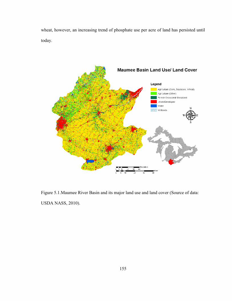
155
wheat, however, an increasing trend of phosphate use per acre of land has persisted until
today.
Figure 5.1.Maumee River Basin and its major land use and land cover (Source of data:
USDA NASS, 2010).
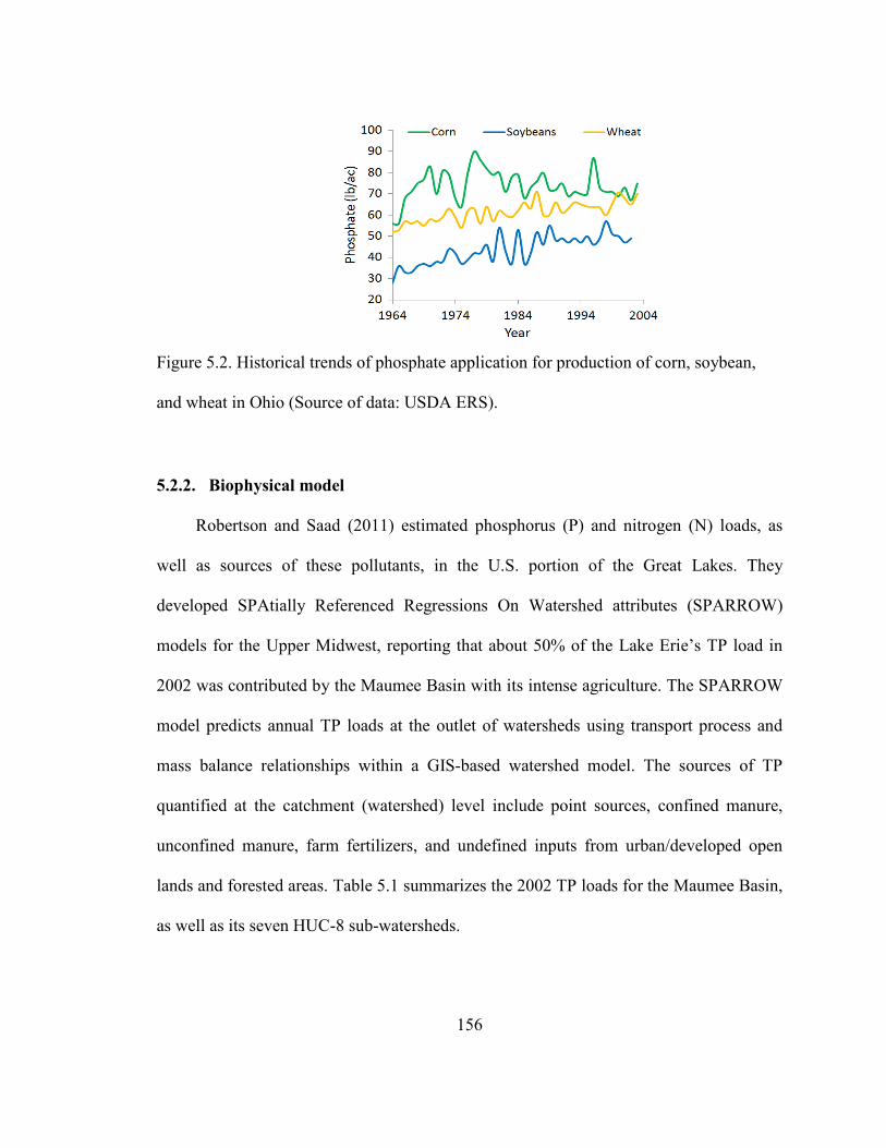
156
Figure 5.2. Historical trends of phosphate application for production of corn, soybean,
and wheat in Ohio (Source of data: USDA ERS).
5.2.2. Biophysical model
Robertson and Saad (2011) estimated phosphorus (P) and nitrogen (N) loads, as
well as sources of these pollutants, in the U.S. portion of the Great Lakes. They
developed SPAtially Referenced Regressions On Watershed attributes (SPARROW)
models for the Upper Midwest, reporting that about 50% of the Lake Erie’s TP load in
2002 was contributed by the Maumee Basin with its intense agriculture. The SPARROW
model predicts annual TP loads at the outlet of watersheds using transport process and
mass balance relationships within a GIS-based watershed model. The sources of TP
quantified at the catchment (watershed) level include point sources, confined manure,
unconfined manure, farm fertilizers, and undefined inputs from urban/developed open
lands and forested areas. Table 5.1 summarizes the 2002 TP loads for the Maumee Basin,
as well as its seven HUC-8 sub-watersheds.
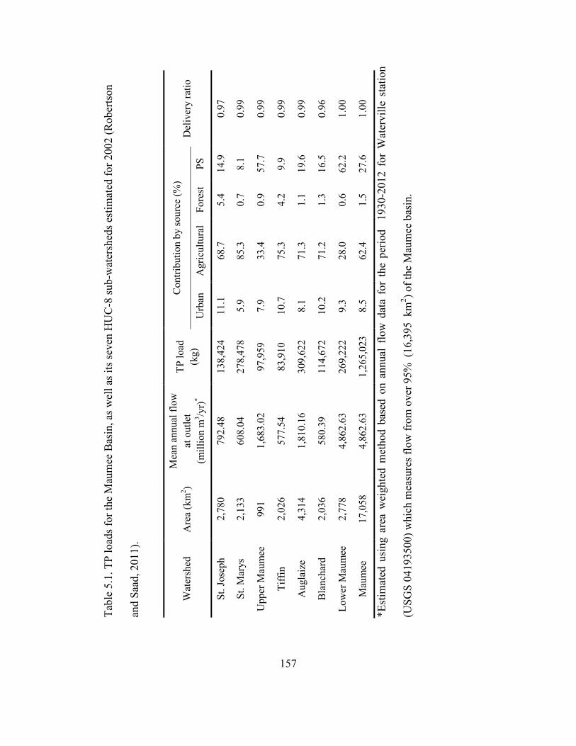
157
Tabl
e 5.
1. T
P lo
ads f
or th
e M
aum
ee B
asin
, as w
ell a
s its
seve
n H
UC
-8 su
b-w
ater
shed
s est
imat
ed fo
r 200
2 (R
ober
tson
and
Saad
, 201
1).
Wat
ersh
ed
Are
a (k
m2 )
Mea
n an
nual
flow
at
out
let
(mill
ion
m3 /y
r)*
TP lo
ad
(kg)
C
ontri
butio
n by
sour
ce (%
) D
eliv
ery
ratio
U
rban
A
gric
ultu
ral
Fore
st PS
St. J
osep
h 2,
780
792.
48
138,
424
11.1
68
.7
5.4
14.9
0.
97
St. M
arys
2,
133
608.
04
278,
478
5.9
85.3
0.
7 8.
1 0.
99
Upp
er M
aum
ee
991
1,68
3.02
97
,959
7.
9 33
.4
0.9
57.7
0.
99
Tiff
in
2,02
6 57
7.54
83
,910
10
.7
75.3
4.
2 9.
9 0.
99
Aug
laiz
e 4,
314
1,81
0.16
30
9,62
2 8.
1 71
.3
1.1
19.6
0.
99
Bla
ncha
rd
2,03
6 58
0.39
11
4,67
2 10
.2
71.2
1.
3 16
.5
0.96
Low
er M
aum
ee
2,77
8 4,
862.
63
269,
222
9.3
28.0
0.
6 62
.2
1.00
Mau
mee
17
,058
4,
862.
63
1,26
5,02
3 8.
5 62
.4
1.5
27.6
1.
00
*Est
imat
ed u
sing
are
a w
eigh
ted
met
hod
base
d on
ann
ual
flow
dat
a fo
r th
e pe
riod
193
0-20
12 f
or W
ater
ville
sta
tion
(USG
S 04
1935
00) w
hich
mea
sure
s flo
w fr
om o
ver 9
5% (
16,3
95 k
m2 ) o
f the
Mau
mee
bas
in.
158
5.2.3. BMP and agro-economic optimization model
The biophysical model provides TP load data at different scales (e.g., sub-
watersheds and watershed), allowing for investigation of watershed scale programs as
compared with zone-based sub-watershed scale programs. The BMP optimization
identifies the least cost BMP set considering urban and agricultural BMPs, using the
model discussed in Chapter 4. The agricultural BMPs considered include constructed
wetlands (CW), conservation tillage (CT), cover crops (CC), and buffer strips (BS)
constructed on privately owned agricultural land. Furthermore, retention basins (RB),
grassed swales and buffer strips (GSB), and detention basins (DB) are considered for
urban areas.
The BMP cost functions given in Table 4.1 were linearized for use in the
optimization model. Furthermore, the model uses TP load data and export coefficients
obtained from the biophysical model (Table 5.1), as well as BMP-specific upper bounds
to provide the minimum-cost BMP set subject to allowable TP load constraints at the
watershed and sub-watershed scale. Tables 5.2 and 5.3 provide BMP specific upper
bounds and area treatment coefficients estimated for the Maumee Basin and its HUC-8
sub-watersheds using the procedures described in Chapter 4.
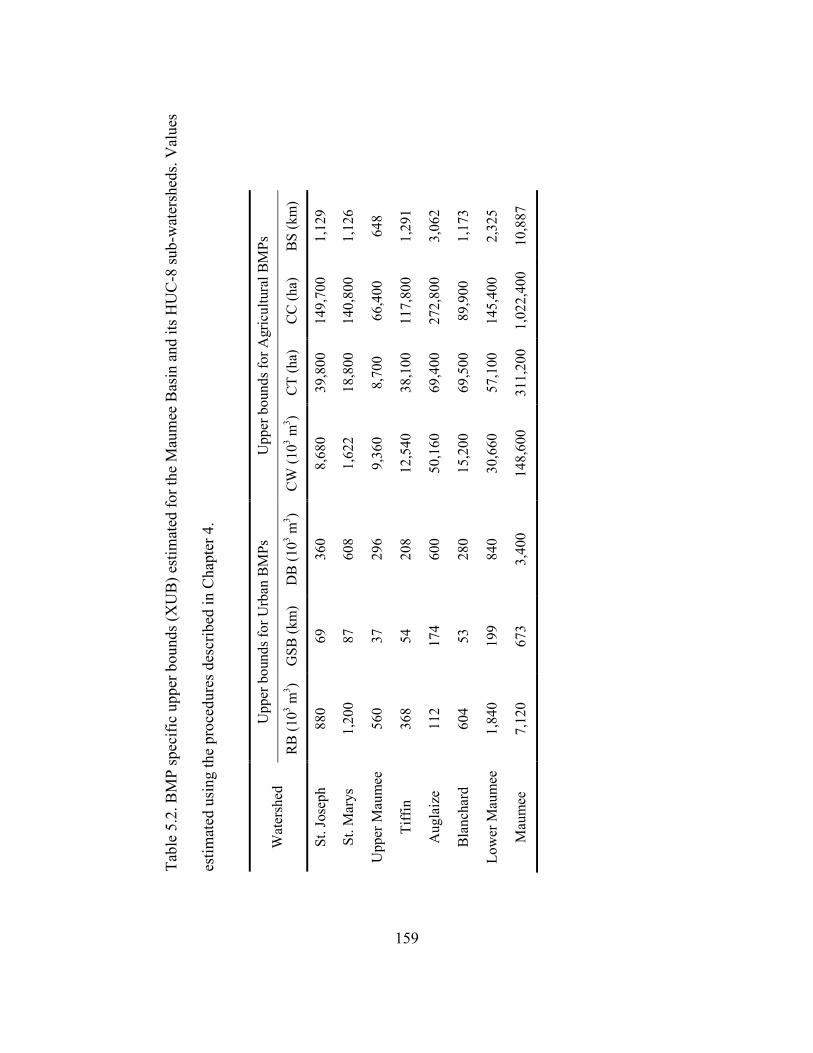
159
Ta
ble
5.2.
BM
P sp
ecifi
c up
per b
ound
s (X
UB
) est
imat
ed fo
r the
Mau
mee
Bas
in a
nd it
s HU
C-8
sub-
wat
ersh
eds.
Val
ues
estim
ated
usi
ng th
e pr
oced
ures
des
crib
ed in
Cha
pter
4.
Wat
ersh
ed
Upp
er b
ound
s for
Urb
an B
MPs
U
pper
bou
nds f
or A
gric
ultu
ral B
MPs
RB
(103 m
3 ) G
SB (k
m)
DB
(103 m
3 ) C
W (1
03 m3 )
CT
(ha)
C
C (h
a)
BS
(km
)
St. J
osep
h 88
0 69
36
0 8,
680
39,8
00
149,
700
1,12
9
St. M
arys
1,
200
87
608
1,62
2 18
,800
14
0,80
0 1,
126
Upp
er M
aum
ee
560
37
296
9,36
0 8,
700
66,4
00
648
Tiff
in
368
54
208
12,5
40
38,1
00
117,
800
1,29
1
Aug
laiz
e 11
2 17
4 60
0 50
,160
69
,400
27
2,80
0 3,
062
Bla
ncha
rd
604
53
280
15,2
00
69,5
00
89,9
00
1,17
3
Low
er M
aum
ee
1,84
0 19
9 84
0 30
,660
57
,100
14
5,40
0 2,
325
Mau
mee
7,
120
673
3,40
0 14
8,60
0 31
1,20
0 1,
022,
400
10,8
87
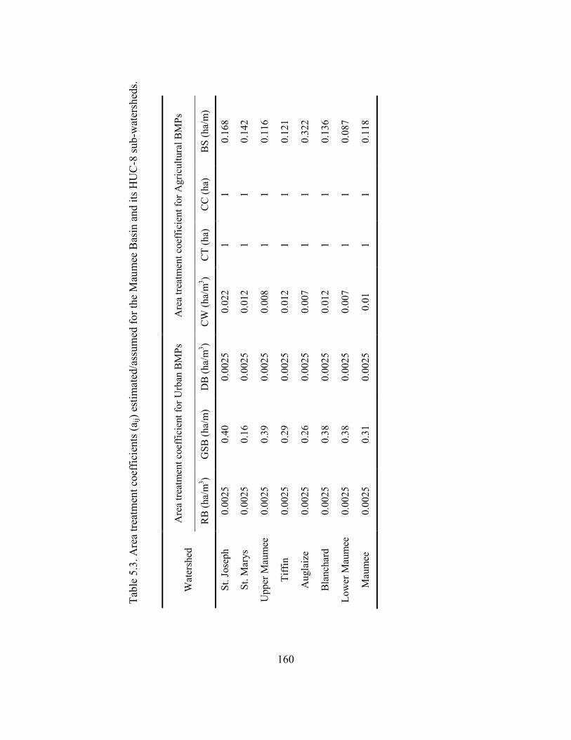
160
Tabl
e 5.
3. A
rea
treat
men
t coe
ffic
ient
s (a ij
) est
imat
ed/a
ssum
ed fo
r the
Mau
mee
Bas
in a
nd it
s HU
C-8
sub-
wat
ersh
eds.
Wat
ersh
ed
Are
a tre
atm
ent c
oeff
icie
nt fo
r Urb
an B
MPs
A
rea
treat
men
t coe
ffic
ient
for A
gric
ultu
ral B
MPs
RB
(ha/
m3 )
GSB
(ha/
m)
DB
(ha/
m3 )
CW
(ha/
m3 )
CT
(ha)
C
C (h
a)
BS
(ha/
m)
St. J
osep
h 0.
0025
0.
40
0.00
25
0.02
2 1
1 0.
168
St. M
arys
0.
0025
0.
16
0.00
25
0.01
2 1
1 0.
142
Upp
er M
aum
ee
0.00
25
0.39
0.
0025
0.
008
1 1
0.11
6
Tiff
in
0.00
25
0.29
0.
0025
0.
012
1 1
0.12
1
Aug
laiz
e 0.
0025
0.
26
0.00
25
0.00
7 1
1 0.
322
Bla
ncha
rd
0.00
25
0.38
0.
0025
0.
012
1 1
0.13
6
Low
er M
aum
ee
0.00
25
0.38
0.
0025
0.
007
1 1
0.08
7
Mau
mee
0.
0025
0.
31
0.00
25
0.01
1
1 0.
118
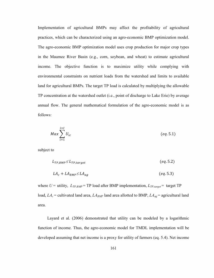
161
Implementation of agricultural BMPs may affect the profitability of agricultural
practices, which can be characterized using an agro-economic BMP optimization model.
The agro-economic BMP optimization model uses crop production for major crop types
in the Maumee River Basin (e.g., corn, soybean, and wheat) to estimate agricultural
income. The objective function is to maximize utility while complying with
environmental constraints on nutrient loads from the watershed and limits to available
land for agricultural BMPs. The target TP load is calculated by multiplying the allowable
TP concentration at the watershed outlet (i.e., point of discharge to Lake Erie) by average
annual flow. The general mathematical formulation of the agro-economic model is as
follows:
𝑀𝑎𝑥�𝑈𝑖𝑐
𝑖=𝐼
𝑖=1
(𝑒𝑞. 5.1)
subject to
𝐿𝑇𝑃,𝐵𝑀𝑃≤ 𝐿𝑇𝑃,𝑡𝑎𝑟𝑔𝑒𝑡 (𝑒𝑞. 5.2)
𝐿𝐴𝑐 + 𝐿𝐴𝐵𝑀𝑃≤ 𝐿𝐴𝑎𝑔 (𝑒𝑞. 5.3)
where U = utility, LTP,BMP = TP load after BMP implementation, LTP,target = target TP
load, LAc = cultivated land area, LABMP land area allotted to BMP, LAag = agricultural land
area.
Layard et al. (2006) demonstrated that utility can be modeled by a logarithmic
function of income. Thus, the agro-economic model for TMDL implementation will be
developed assuming that net income is a proxy for utility of farmers (eq. 5.4). Net income
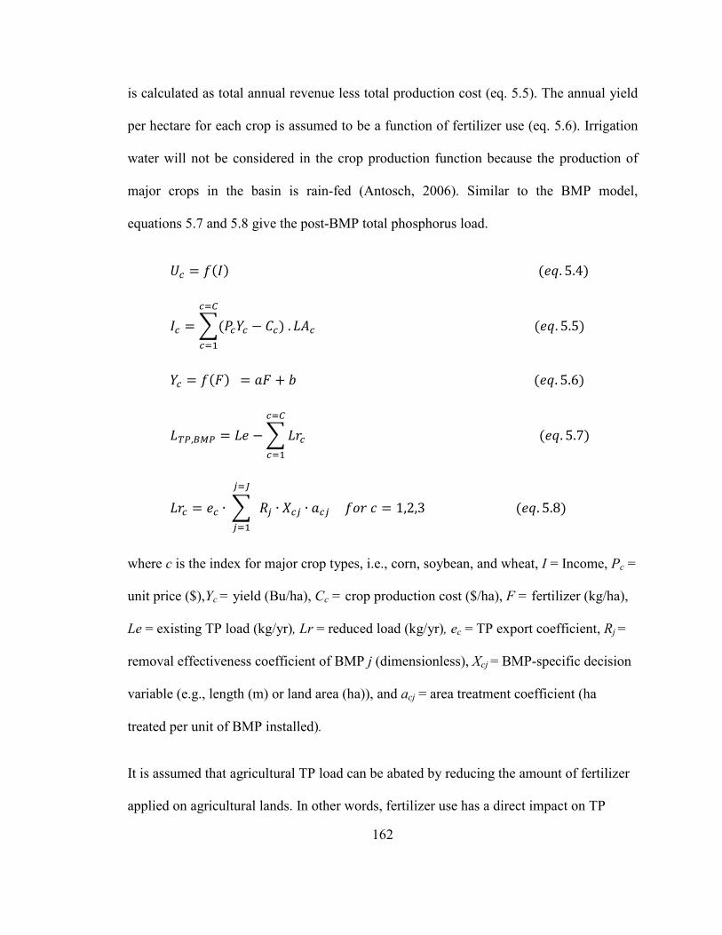
162
is calculated as total annual revenue less total production cost (eq. 5.5). The annual yield
per hectare for each crop is assumed to be a function of fertilizer use (eq. 5.6). Irrigation
water will not be considered in the crop production function because the production of
major crops in the basin is rain-fed (Antosch, 2006). Similar to the BMP model,
equations 5.7 and 5.8 give the post-BMP total phosphorus load.
𝑈𝑐 = 𝑓(𝐼) (𝑒𝑞. 5.4)
𝐼𝑐 = �(𝑃𝑐𝑌𝑐 − 𝐶𝑐
𝑐=𝐶
𝑐=1
) . 𝐿𝐴𝑐 (𝑒𝑞. 5.5)
𝑌𝑐 = 𝑓(𝐹) = 𝑎𝐹 + 𝑏 (𝑒𝑞. 5.6)
𝐿𝑇𝑃,𝐵𝑀𝑃 = 𝐿𝑒 −�𝐿𝑟𝑐
𝑐=𝐶
𝑐=1
(𝑒𝑞. 5.7)
𝐿𝑟𝑐 = 𝑒𝑐 ∙ � 𝑅𝑗 ∙ 𝑋𝑐𝑗 ∙ 𝑎𝑐𝑗
𝑗=𝐽
𝑗=1
𝑓𝑜𝑟 𝑐 = 1,2,3 (𝑒𝑞. 5.8)
where c is the index for major crop types, i.e., corn, soybean, and wheat, I = Income, Pc =
unit price ($),Yc = yield (Bu/ha), Cc = crop production cost ($/ha), F = fertilizer (kg/ha),
Le = existing TP load (kg/yr), Lr = reduced load (kg/yr), ec = TP export coefficient, Rj =
removal effectiveness coefficient of BMP j (dimensionless), Xcj = BMP-specific decision
variable (e.g., length (m) or land area (ha)), and acj = area treatment coefficient (ha
treated per unit of BMP installed).
It is assumed that agricultural TP load can be abated by reducing the amount of fertilizer
applied on agricultural lands. In other words, fertilizer use has a direct impact on TP
163
export coefficients. Fertilizer use for different crops for the year 2002 is considered as the
reference for adjusting the export coefficients (eq. 5.9).
𝑒𝑐 = (𝐹𝑐/𝐹𝑐,2002) × 𝑒𝑐,2002 (𝑒𝑞. 5.9)
The total production cost comprises the regular production and operating cost, as
well as the earmarked fertilizer tax to cover BMP cost. Assuming the funds for BMP
implementation will be generated through imposition of a cost covering input (i.e.,
fertilizer use) tax, the cost function can be written as follows:
𝐶𝑐 = 𝐶𝑟𝑐 + 𝑇𝑐 (𝑒𝑞. 5.10)
𝑇𝑐 =𝐶𝐵𝑀𝑃,𝑐 𝐹
(𝑒𝑞. 5.11)
𝐶𝐵𝑀𝑃,𝑐 = �𝐶𝐵𝑀𝑃,𝑗. �𝑋𝑗�𝑗=𝐽
𝑗=1
(𝑒𝑞. 5.12)
where Crc = regular production and operating costs ($/ha-yr) including the cost of seed,
labor, and interest on operating capital, Tc = fertilizer use tax for crop c ($/kg-ha), CBMP =
cost of BMP ($), j = BMP type, including constructed wetland, conservation tillage,
cover crop, buffer strip (J = 4).
The agronomic data for deriving the crop production functions were obtained from
the United States Department of Agriculture (USDA ERS, 2012). The data sets include
time series of corn, soybeans, and wheat yield (Bu/ha), acreage, fertilizer use (kg/ha),
total economic costs of production ($/ha), price of the crop ($/Bu), and fertilizer price
($/kg-ha) was estimated using the cost of fertilizer ($) and amount of fertilizer applied per
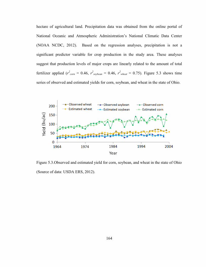
164
hectare of agricultural land. Precipitation data was obtained from the online portal of
National Oceanic and Atmospheric Administration’s National Climatic Data Center
(NOAA NCDC, 2012). Based on the regression analyses, precipitation is not a
significant predictor variable for crop production in the study area. These analyses
suggest that production levels of major crops are linearly related to the amount of total
fertilizer applied (r2corn = 0.46, r2
soybean = 0.46, r2wheat = 0.75). Figure 5.3 shows time
series of observed and estimated yields for corn, soybean, and wheat in the state of Ohio.
Figure 5.3.Observed and estimated yield for corn, soybean, and wheat in the state of Ohio
(Source of data: USDA ERS, 2012).
165
5.3. Results and discussion
5.3.1. Scale dependence of BMP implementation efficiency
Applying the BMP optimization model at the watershed and sub-watershed scales
provides insights for improving the cost efficiency of a TMDL program. Two
implementation scenarios have been considered. In the first scenario, sub-watershed scale
BMP implementation across individual sub-watersheds, the least-cost BMP set was
obtained assuming that there is no interaction between sub-watersheds in terms of BMP
implementation. However, the effect of the applied BMP set in an upstream sub-
watershed was propagated downstream. This scenario represents lack of coordination in
terms of BMP implementation across sub-watersheds. In the second scenario, a more
flexible sub-watershed scale BMP implementation was modeled to meet the TP target
concentration at the outlet of each sub-watershed while meeting the Maumee Basin’s TP
concentration target at the point of discharge to Lake Erie. In other words, this scenario
allows for application of additional BMPs in an upstream sub-watershed to facilitate
attainment of the water quality target at the outlet of a downstream sub-watershed. This
scenario was named sub-watershed scale BMP implementation across the Maumee Basin,
representing coordinated BMP implementation. Figure 5.4 shows the seven sub-
watersheds in the Maumee Basin, and Table 5.4 provides land use characteristics of each
sub-watershed and their water quality target.
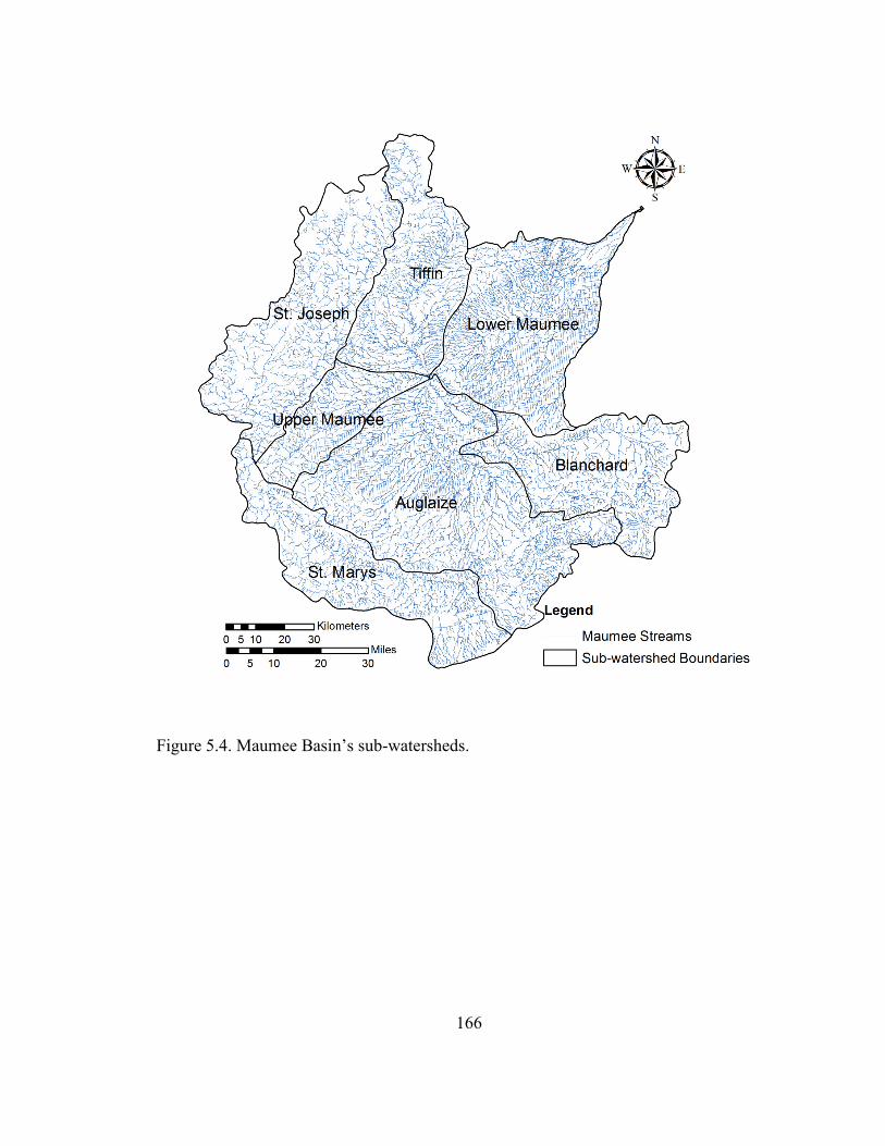
166
Figure 5.4. Maumee Basin’s sub-watersheds.
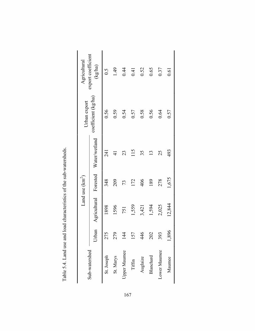
167
Tabl
e 5.
4. L
and
use
and
load
cha
ract
eris
tics o
f the
sub-
wat
ersh
eds.
Sub-
wat
ersh
ed
Land
use
(km
2 ) U
rban
exp
ort
coef
ficie
nt (k
g/ha
)
Agr
icul
tura
l ex
port
coef
ficie
nt
(kg/
ha)
Urb
an
Agr
icul
tura
l Fo
rest
ed
Wat
er/w
etla
nd
St. J
osep
h 27
5 18
98
348
241
0.56
0.
5
St. M
arys
27
9 15
96
209
41
0.59
1.
49
Upp
er M
aum
ee
144
751
73
23
0.54
0.
44
Tiff
in
157
1,55
9 17
2 11
5 0.
57
0.41
Aug
laiz
e 44
6 3,
421
406
35
0.58
0.
52
Bla
ncha
rd
202
1,59
4 18
9 13
0.
56
0.65
Low
er M
aum
ee
393
2,02
5 27
8 25
0.
64
0.37
Mau
mee
1,
896
12,8
44
1,67
5 49
3 0.
57
0.61
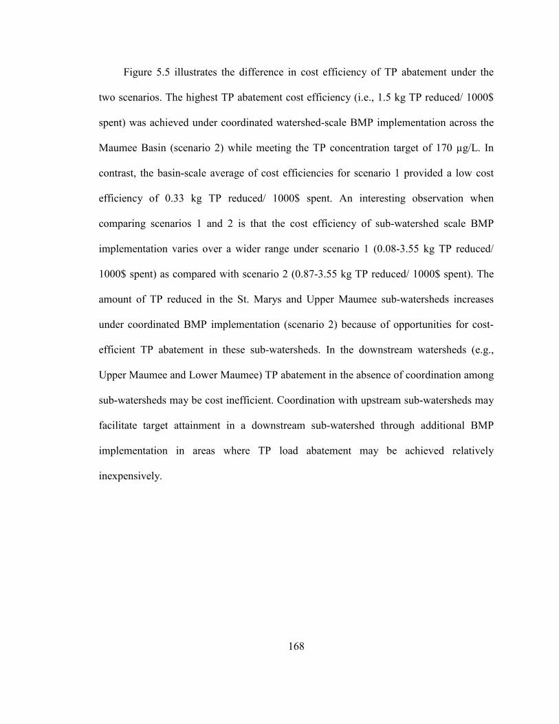
168
Figure 5.5 illustrates the difference in cost efficiency of TP abatement under the
two scenarios. The highest TP abatement cost efficiency (i.e., 1.5 kg TP reduced/ 1000$
spent) was achieved under coordinated watershed-scale BMP implementation across the
Maumee Basin (scenario 2) while meeting the TP concentration target of 170 µg/L. In
contrast, the basin-scale average of cost efficiencies for scenario 1 provided a low cost
efficiency of 0.33 kg TP reduced/ 1000$ spent. An interesting observation when
comparing scenarios 1 and 2 is that the cost efficiency of sub-watershed scale BMP
implementation varies over a wider range under scenario 1 (0.08-3.55 kg TP reduced/
1000$ spent) as compared with scenario 2 (0.87-3.55 kg TP reduced/ 1000$ spent). The
amount of TP reduced in the St. Marys and Upper Maumee sub-watersheds increases
under coordinated BMP implementation (scenario 2) because of opportunities for cost-
efficient TP abatement in these sub-watersheds. In the downstream watersheds (e.g.,
Upper Maumee and Lower Maumee) TP abatement in the absence of coordination among
sub-watersheds may be cost inefficient. Coordination with upstream sub-watersheds may
facilitate target attainment in a downstream sub-watershed through additional BMP
implementation in areas where TP load abatement may be achieved relatively
inexpensively.
169
Figure 5.5. Comparison of cost efficiency between sub-watershed scale and watershed
scale implementation of least-cost BMP set.
170
Agricultural BMPs dominate the least-cost BMP set for different sub-watersheds, as
may be expected because agriculture is the primary largest land use in the study area.
Agricultural buffer strips and constructed wetlands, as well as tillage practices, can result
in significant TP load abatement in each of the Maumee Basin’s sub-watersheds. In
particular, development and proper maintenance of agricultural buffer strips should be
considered as an important agricultural BMP. Potential TP load abatements resulting
from BMPs implemented on sub-watershed scales across individual sub-watersheds and
across the entire Maumee Basin, scenarios 1 and 2, are shown in Figure 5.6. The smallest
TP load abatements occur in upstream sub-watersheds such as St. Joseph and Blanchard.
At the current scale of analysis, Tiffin meets the TP concentration target without BMPs.
In contrast, large TP export coefficients for St. Marys and Auglaize result in intensive
BMP implementation in these sub-watersheds. Similarly, although BMP implementation
may significantly reduce TP emission throughout the basin, the Lower Maumee sub-
watershed will require extensive BMP implementation, in part because it receives a large
TP load (~339,000 kg/yr) from upstream sub-watersheds. As shown in Figure 5.5b, a
more flexible BMP implementation scheme can facilitate additional TP load abatement in
areas with higher cost-efficiency (e.g., St. Joseph and Auglaize), denoting the importance
of a basin approach to BMP implementation. Under scenario 2, the load abatement in
upstream watersheds increased, facilitating the attainment of the TP concentration target
of 170 µg/L in downstream sub-watersheds.
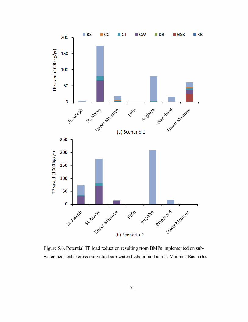
171
Figure 5.6. Potential TP load reduction resulting from BMPs implemented on sub-
watershed scale across individual sub-watersheds (a) and across Maumee Basin (b).
172
5.3.2. Fertilizer tax as a TP abatement policy
The use of fertilizer tax as a potential TP abatement policy was investigated through
maximization of net basin scale agricultural income under three scenarios: (1) fertilizer
tax imposition when agricultural land may be partially cultivated (land under cultivation
is a decision variable); (2) fertilizer tax imposition when at least 50% of agricultural land
is cultivated; and (3) BMP cost is fully covered by external funds. Scenarios 1 and 2
capture the effects of fully internalizing the cost of TP load emissions considering the
effect of land constraint, whereas scenario 3 represents a case where TP load abatement is
achieved through government subsidy and without significant impacts on agricultural
sector profits. The analysis was conducted at the Maumee Basin scale assuming that all
the agricultural lands will be allotted to cultivation of corn, soybeans, and wheat. The
land under cultivation of corn, soybeans, and wheat was scaled up to cover the entire
agricultural area based on the 2010 cultivation area available from Crop Data Layer
(CDL) (USDA NASS, 2010). As assumption was made that agricultural TP export
coefficient comprises contributions from the three major crops. Average TP export
coefficients for each of the three different crops were estimated based on fertilizer use
and cultivation area such that the collective effect of the export coefficients would give
the agricultural TP load estimated by SPARROW. A linear relationship was assumed
relating the export coefficients to total fertilizer use for each crop. Table 5.4 provides the
basin scale data for Maumee Basin’s major crops including available land area for
cultivation, agro-economic data, and average TP export coefficients.
The analysis results for the three noted policies are summarized in Table 5.5.
Internalization of the cost of TP load abatement has a significant direct impact on
173
agricultural production through decisions about cultivated land area and fertilizer use.
The agricultural sector will strive to maintain the highest possible yield while meeting the
constraints of the TP load abatement policy. Under the extreme policy of full
internalization of TP load abatement cost through fertilizer tax imposition using land as a
decision variable (policy scenario 1), only a very small proportion of the available land is
cultivated for soybeans (1.45%) and wheat (1.39%), while most available land was used
for corn production (82.22%). When an additional constraint is imposed requiring the use
of at least 50% of available agricultural lands for different crops (policy scenario 2),
results indicate a reduction of fertilizer use for corn while fertilizer use for soybeans and
wheat was at the lower bound, thus reducing the crop yields. Upper and lower bounds of
fertilizer use for different crops were estimated with reference to historical fertilizer use
using data from the United States Department of Agriculture’s Economic Research
Service (USDA ERS, 2012).
In contrast to abatement cost internalization policies, TP load abatement through
external funds for BMP implementation (policy scenario 3) will have a minimal impact
on the agricultural production (Table 5.5). Under this extreme scenario, all the available
lands for the three crops were cultivated, and maximum yield was achieved through
application of fertilizer at the upper bound of fertilizer use. A significant amount of TP
load from different crop lands was reduced through implementation of agricultural
BMPs, namely agricultural buffer strips and conservation tillage, and cover crops.
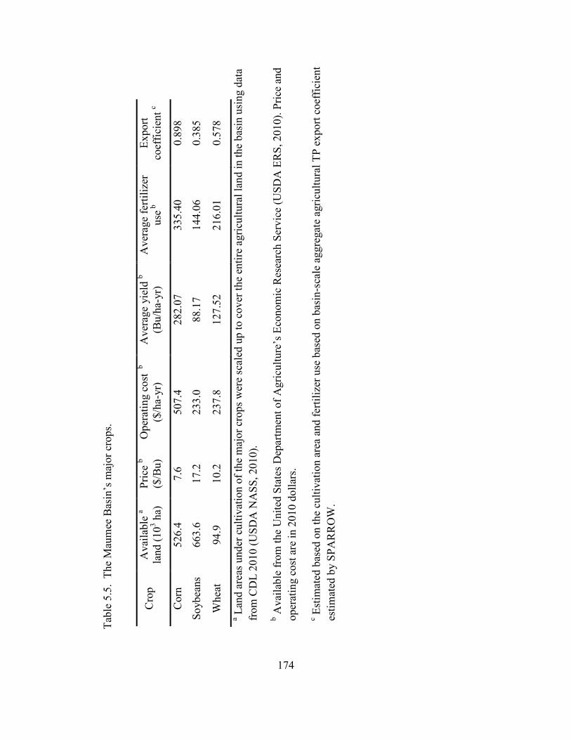
174
Tabl
e 5.
5. T
he M
aum
ee B
asin
’s m
ajor
cro
ps.
a Lan
d ar
eas u
nder
cul
tivat
ion
of th
e m
ajor
cro
ps w
ere
scal
ed u
p to
cov
er th
e en
tire
agric
ultu
ral l
and
in th
e ba
sin
usin
g da
ta
from
CD
L 20
10 (U
SDA
NA
SS, 2
010)
.
b Ava
ilabl
e fr
om th
e U
nite
d St
ates
Dep
artm
ent o
f Agr
icul
ture
’s E
cono
mic
Res
earc
h Se
rvic
e (U
SDA
ER
S, 2
010)
. Pric
e an
d op
erat
ing
cost
are
in 2
010
dolla
rs.
c Est
imat
ed b
ased
on
the
culti
vatio
n ar
ea a
nd fe
rtiliz
er u
se b
ased
on
basi
n-sc
ale
aggr
egat
e ag
ricul
tura
l TP
expo
rt co
effic
ient
es
timat
ed b
y SP
AR
RO
W.
Cro
p A
vaila
ble
a la
nd (1
03 ha)
Pr
ice
b ($
/Bu)
O
pera
ting
cost
b
($/h
a-yr
) A
vera
ge y
ield
b (B
u/ha
-yr)
A
vera
ge fe
rtiliz
er
use b
Ex
port
coef
ficie
nt c
Cor
n 52
6.4
7.6
507.
4 28
2.07
33
5.40
0.
898
Soyb
eans
66
3.6
17.2
23
3.0
88.1
7 14
4.06
0.
385
Whe
at
94.9
10
.2
237.
8 12
7.52
21
6.01
0.
578
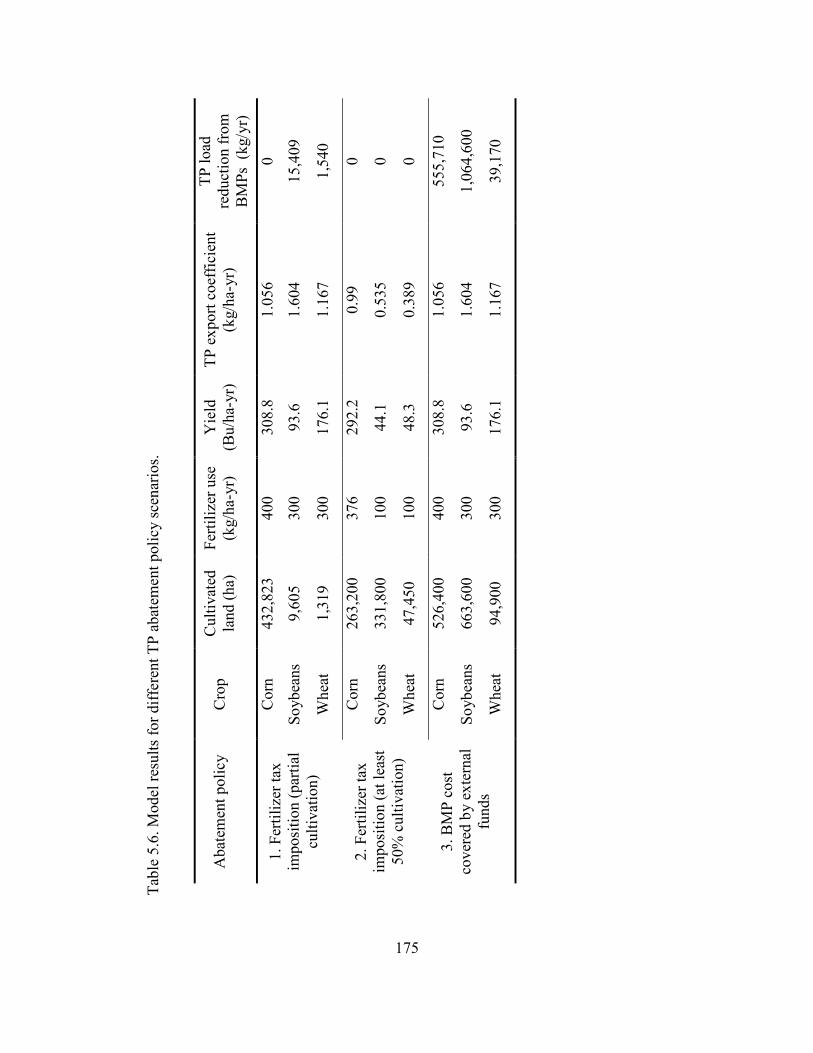
175
Tabl
e 5.
6. M
odel
resu
lts fo
r diff
eren
t TP
abat
emen
t pol
icy
scen
ario
s.
Aba
tem
ent p
olic
y C
rop
Cul
tivat
ed
land
(ha)
Fe
rtiliz
er u
se
(kg/
ha-y
r)
Yie
ld
(Bu/
ha-y
r)
TP e
xpor
t coe
ffic
ient
(k
g/ha
-yr)
TP
load
re
duct
ion
from
B
MPs
(kg
/yr)
1. F
ertil
izer
tax
impo
sitio
n (p
artia
l cu
ltiva
tion)
Cor
n 43
2,82
3 40
0 30
8.8
1.05
6 0
Soyb
eans
9,
605
300
93.6
1.
604
15,4
09
Whe
at
1,31
9 30
0 17
6.1
1.16
7 1,
540
2. F
ertil
izer
tax
impo
sitio
n (a
t lea
st
50%
cul
tivat
ion)
Cor
n 26
3,20
0 37
6 29
2.2
0.99
0
Soyb
eans
33
1,80
0 10
0 44
.1
0.53
5 0
Whe
at
47,4
50
100
48.3
0.
389
0
3. B
MP
cost
co
vere
d by
ext
erna
l fu
nds
Cor
n 52
6,40
0 40
0 30
8.8
1.05
6 55
5,71
0
Soyb
eans
66
3,60
0 30
0 93
.6
1.60
4 1,
064,
600
Whe
at
94,9
00
300
176.
1 1.
167
39,1
70
176
Figure 5.7 shows the basin scale net economic benefit (profit) to the agricultural
sector as a surrogate for utility. The highest profit is achieved under the extreme policy of
TP load abatement through external funds (policy scenario 3), whereas internalization of
TP load abatement cost with the constraint requiring use of at least 50% of available
lands (policy scenario 2) resulted in the lowest utility. This is because application of
upper bounds of fertilizer under policy scenario 3 provides the highest yield and the cost
of TP abatement through agricultural BMP implementation is not incurred by the
agricultural sector. The requirement for use of at least 50% of available agricultural lands
creates a high fertilizer cost component coupled with low yields, indicating sub-
optimality of inflexible policies with respect to cultivate land area. Full internalization of
TP abatement cost allowing partial cultivation of crops (policy scenario 1) resulted in
about 50% reduction in profit compared with scenario 3 because the optimal solution is to
produce a high yield crop (i.e., corn) using upper bound of fertilizer use. Essentially,
under this policy scenario, the agricultural sector opts to meet the TP load requirement
through significant curtailment of cultivation of soybeans and wheat than extensive BMP
implementation.
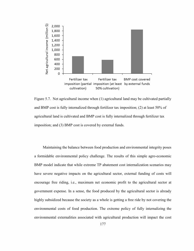
177
Figure 5.7. Net agricultural income when (1) agricultural land may be cultivated partially
and BMP cost is fully internalized through fertilizer tax imposition; (2) at least 50% of
agricultural land is cultivated and BMP cost is fully internalized through fertilizer tax
imposition; and (3) BMP cost is covered by external funds.
Maintaining the balance between food production and environmental integrity poses
a formidable environmental policy challenge. The results of this simple agro-economic
BMP model indicate that while extreme TP abatement cost internalization scenarios may
have severe negative impacts on the agricultural sector, external funding of costs will
encourage free riding, i.e., maximum net economic profit to the agricultural sector at
government expense. In a sense, the food produced by the agricultural sector is already
highly subsidized because the society as a whole is getting a free ride by not covering the
environmental costs of food production. The extreme policy of fully internalizing the
environmental externalities associated with agricultural production will impact the cost
178
and abundance of food. However, as the world prepares to double food production by
2050 (Tilman et al., 2002), partial internalization of environmental externalities is
necessary because it can reduce the environmental impacts of agricultural production.
Alleviating the impact of the environmental cost internalization on agricultural
production will require government intervention in the form of subsidies and incentive
programs, as well contribution from society as a whole through paying a higher price for
food in order to partially cover the environmental costs.
Although TP load abatement through external funds will be the most desirable
policy to the agricultural sector and consumers of agricultural products, the cost of
implementing this policy on the national level may be overwhelming. Recognizing over-
application of fertilizers as one of the root causes of eutrophication, agricultural BMP
implementation may only provide a short-term solution by temporarily capturing the
nutrients. The sustainable solution to agricultural nutrient loads is to adapt fertilizer
application to the carrying capacity of the water bodies and in amounts that can be taken
up by plants and assimilated by BMPs.
5.4. Future work
Future research investigating the application of a fertilizer tax as a TP abatement
policy will consider analysis at the scale of seven individual sub-watersheds that
comprise the Maumee River watershed. At the basin scale, the collective impact of
different sub-watersheds should be considered when optimizing the fertilizer tax to cover
the cost of an agricultural BMP plan for compliance with target total TP loads.
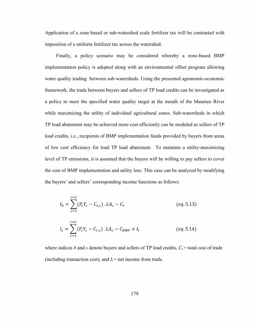
179
Application of a zone-based or sub-watershed scale fertilizer tax will be contrasted with
imposition of a uniform fertilizer tax across the watershed.
Finally, a policy scenario may be considered whereby a zone-based BMP
implementation policy is adopted along with an environmental offset program allowing
water quality trading between sub-watersheds. Using the presented agronomic-economic
framework, the trade between buyers and sellers of TP load credits can be investigated as
a policy to meet the specified water quality target at the mouth of the Maumee River
while maximizing the utility of individual agricultural zones. Sub-watersheds in which
TP load abatement may be achieved more cost efficiently can be modeled as sellers of TP
load credits, i.e., recipients of BMP implementation funds provided by buyers from areas
of low cost efficiency for load TP load abatement. To maintain a utility-maximizing
level of TP emissions, it is assumed that the buyers will be willing to pay sellers to cover
the cost of BMP implementation and utility loss. This case can be analyzed by modifying
the buyers’ and sellers’ corresponding income functions as follows:
𝐼𝑏 = �(𝑃𝑐𝑌𝑐 − 𝐶𝑟,𝑐
𝑐=𝐶
𝑐=1
) . 𝐿𝐴𝑐 − 𝐶𝑡 (𝑒𝑞. 5.13)
𝐼𝑠 = �(𝑃𝑐𝑌𝑐 − 𝐶𝑟,𝑐
𝑐=𝐶
𝑐=1
) .𝐿𝐴𝑐 − 𝐶𝐵𝑀𝑃 + 𝐼𝑡 (𝑒𝑞. 5.14)
where indices b and s denote buyers and sellers of TP load credits, Ct = total cost of trade
(including transaction cost), and It = net income from trade.
180
5.5. Conclusions
A BMP optimization model was developed and applied to the Maumee Basin to
provide insights for NPS TP load reduction in the Maumee Basin. A coordinated basin
scale BMP implementation whereby the target TP concentration of 170 µg/L at the outlet
of the Maumee Basin can be achieved by coordinated BMP implementation across the
watershed is found to be cost-efficient. In terms of cost-efficiency and feasibility of
meeting the target, this BMP implementation scheme is superior to a case where
individual sub-watersheds attempt to meet the outlet TP concentration target without
coordination among other sub-watersheds. However, individual sub-watersheds, as is the
case in the Maumee Basin, may need to reduce their TP load due to local water quality
concerns. If this is the case, a coordinated sub-watershed scale BMP implementation may
be recommended whereby meeting the TP concentration target at the outlet of a
downstream watershed may be facilitated through implementation of additional BMPs in
upstream watersheds.
Implementation of agricultural BMPs may be unaffordable to the agricultural sector
because it significantly reduces the utility of the agricultural production. However,
reemergence of severe nuisance algal blooms, is an indication of the need for more
aggressive TMDL implementation policies. Market-based policy instruments may
provide a more flexible means of addressing NPS pollution as compared with command-
and-control approaches. Future research should explore the potential for imposition of a
zone-based fertilizer tax, as well as environmental offset programs to facilitate NPS TP
abatement.
181
5.6. References
Antosch, L.M. (2006). Ohio irrigation assessment. Ohio Farm Bureau.
<ftp://ftp.dnr.state.oh.us/Soil_&_Water_Conservation/Bleim/Irrigation/Irrigation-
Assessment.pdf> (accessed on Oct. 21, 2012).
Boyd, J. (2003). Water pollution taxes: a good idea doomed to failure?. Public Finance
Management 3(1), 34–66.
Chapra, S., Dolan, D.M. (2012). Great Lakes total phosphorus revisited: 2. Mass balance
modeling. Journal of Great Lakes Research 38, 741-754.
Ekins, R. (1999). European environmental taxes and charges: recent experience, issues
and trends. Ecological Economics 31, 39– 62.
Hsieh, C.D., Yang, W.F. (2007). Optimal nonpoint source pollution control strategies for
a reservoir watershed in Taiwan. Journal of Environmental Management 85, 908–
917.
Lake Erie LaMP (2009). Status of nutrients in the Lake Erie Basin. Prepared for the Lake
Erie LaMP Management Committee.
<http://www.epa.gov/lakeerie/erie_nutrient_2010.pdf > (accessed on Oct. 10,
2012)
Layard, R., Mayaraz, G., Nickell, S. (2006). The Marginal Utility of Income. Mimeo,
London School of Economics.
Ludsin, S.A., Kershner, M.W., Blocksom, K.A., Knight, R.L., Stein, R.A., (2001). Life
after death in Lake Erie: nutrient controls drive fish species richness,
rehabilitation. Ecological Applications 11, 731-46.
182
Makarewicz, J. C., Bertram, P. (1991). Evidence for the restoration of the Lake Erie
ecosystem. BioScience 41,216-223.
National Oceanic and Atmospheric Administration National Climatic Data Center (2012).
< http://www.ncdc.noaa.gov/oa/climate/climatedata.html> (accessed on Oct. 5,
2012).
Ohio EPA (1999), Association between nutrients, habitat, and the aquatic biota in Ohio
rivers and streams, Ohio EPA Technical Bulletin MAS/1999-1-1, Ohio EPA,
Division of Surface Water, Monitoring and Assessment Section, Columbus, Ohio.
Ohio EPA. (2010). Ohio Lake Erie phosphorus task force final report.
<http://www.epa.ohio.gov/portals/35/lakeerie/ptaskforce/Task_Force_Final_Repo
rt_April_2010.pdf> (accessed on Oct. 5, 2012).
Plourde, J. D. (2012). Assessing changes and drivers of crop rotation patterns and their
implications for nitrogen loading in the United States. MS Thesis, Purdue
University, West Lafayette, IN.
Robertson, D. M.; Saad, D. A. (2011). Nutrient inputs to the Laurentian Great Lakes by
source and watershed estimated using SPARROW watershed models. Journal of
American Water Resources Association 47(5), 1011-1033.
Selman, M., Greenhalgh, S., Branosky, E., Jones, C., Guiling, J. (2009). Water quality
trading programs: An international overview. WRI Issue Brief, World Resources
Institute, Washington, D.C.
Shortle, J., Horan, R. (2001). The Economics of Nonpoint Pollution Control. Journal of
Economic Surveys 15(3), 255–289.
183
Tilman, D., Cassman, K.G., Matson, P.A., Naylor, R., Polasky, S. (2002). Agricultural
sustainability and intensive production practices. Nature 418, 671–677.
Turner, R.K., Georgiou, S., Gren, I., Wulff, F., Barrett, S., Söderqvist, T., Bateman, I.J.,
Folke, C., Langaas, S., Zylicz, T., Karl-Goran Mäler, K., Markowska, A. (1999).
Managing nutrient fluxes and pollution in the Baltic: an interdisciplinary
simulation study. Ecological Economics 30, 333–352.
United States Department of Agriculture Economic Research Service (2012). Available
online: http://www.ers.usda.gov/data-products.aspx (Accessed in October 2012).
United States Department of Agriculture National Agricultural Statistics Service (2012).
< http://www.nass.usda.gov/research/Cropland/SARS1a.htm> (accessed on
October 10, 2012).
Zaring, D. (1996). Agriculture, nonpoint source pollution, and regulatory control: The
clean water act’s bleak present and future. Harvard Environmental Law Review
20, 515-545.
184
Chapter 6 – Conclusions and Future Research
6.1. Need for systems thinking
Water resources systems involve natural and anthropogenic processes that are
complex, dynamic, and spatially variable. Previous experiences of unsuccessful or
unsustainable watershed planning and management practices manifest how a lack of
understanding of water resources subsystems can cause environmental disasters as well
as socioeconomic problems affecting humans’ wellbeing. Water resources modeling has
become a commonplace tool for water resources system design, planning, and
management at an affordable cost and within a reasonable timeframe. Over the past
decades, water resources systems models have evolved from describing only physical
processes to describing the interaction of social, economic, and environmental systems
objectives in support of decision making. The gradual shift from merely employing
engineering-based simulation models to applying integrated hydroeconomic models, and
more recently multi-criteria/multi-objective decision making and conflict resolution
models, is an indicator of promising changes in the traditional paradigm for the
application of water resources models. More holistic understanding of water resources
systems and improved abilities to predict and plan for future impacts are likely to lead to
more sustainable watershed planning and management decisions.
185
6.2. System dynamics and water resources modeling
This dissertation illustrated the role of the systems thinking paradigm in water
resources planning and decision making, demonstrating qualitative, as well as
quantitative capabilities of system dynamics modeling in facilitating holistic water
resources modeling and policy making. Using tangible water resources examples, the
fundamentals of system dynamics, including causal relationships, CLDs, SFDs, and water
resources system archetypes, were illustrated. Applying a systems thinking paradigm to
water resources modeling is critical when formulating strategic-level water management
policies and plans, considering that a traditional linear thinking paradigm may lead to
quick-fix solutions that fail to address key drivers of the problem. Systems thinking and
system dynamics modeling can help water resources decision makers comprehend the
interactions among various interlinked sub-systems of a water resources system which
drive its long-run dynamic behavior.
A wave of water resources modeling efforts using system dynamics has emerged in
the past two decades as modelers strive to capture the main drivers of water resources
problems, including interrelationships between disparate natural, technological, and
socio-economic subsystems. The approach has proven useful for providing valuable
insights into problems and systems’ long-run behavior at the strategic level. In addition,
system dynamics models’ transparent structure and convenient sensitivity analysis make
them practical tools for participatory modeling, policy screening, and high-level adaptive
management. Object-oriented modeling tools enable transparent system dynamics
modeling by providing generic building blocks to capture systems’ nonlinear behavior.
186
However, the current versions of these modeling tools tend to be limited in terms of
flexibility of programming.
Compared to other modeling approaches, a significant advantage of system
dynamics is that when systems are not too complicated, the CLD and SFD of the system
can help determine the qualitative behavior of many variables, even before quantitative
(numerical) modeling begins. Furthermore, water managers can use knowledge of
archetypal behavior (e.g., Limits to Growth, Fixes that Backfire, Success to the
Successful, Tragedy of the Commons, and Growth and Underinvestment) to recognize
common patterns of dynamic behavior in water resources systems. Thus, understanding
the underlying structure of water resources systems can help avoid unintended
consequences and unsustainable development trajectories by detecting the root causes of
problematic trends and identifying potential corrective measures.
Perhaps the most significant aspect of system dynamics is its ability to facilitate
multi-disciplinary, multi-sectoral, and participatory modeling of integrated systems. At
the strategic level, when studying water resources systems with disparate dynamic
variables, emphasis should be placed on trend identification and pattern recognition
rather than exact quantitative predictions. In this way, decision makers can learn about
the potential impacts of their decisions on different natural and socio-economic
subsystems using “what-if” analyses. Optimization methods may also be applied to
develop prescriptive plans and facilitate trade-off analysis. Thus, system dynamics
models are developed to promote understanding of general trends and the reasons behind
them. Nonetheless, from the standpoint of integrated water resources planning and
management, system dynamics models can improve understanding of the big picture,
187
while specific plans and designs should be studied in more detail using hydroeconomic
models and engineering-based watershed process models to ensure informed decisions.
6.3. A systems approach to water quality management
The United States Clean Water Act provides a good opportunity for applying the
systems approach to water quality management. The CWA requires each state to identify
the main pollutant(s) of concern impairing water bodies. The states should meet water
quality standards using TMDLs, i.e., a written plan quantifying allowable levels of load
allocation (NPS pollution) and waste-load allocation (PS pollution). Furthermore, a
margin of safety is warranted to compensate for lack of knowledge as to relationship
between pollutant inputs and water quality.
Within this framework, system dynamics modeling was applied to identify and
simulate the system structure driving the long-term eutrophication-recovery trend of Lake
Allegan, Michigan to provide insights into policies for mitigating impairment. Once a
potential strategy (e.g., TP load mitigation in agricultural and urban areas) has been
identified, it can be investigated in more detail using optimization modeling in order to
find cost-effective policies to address the problem. The Lake Allegan case study
illustrated how simple system dynamics models can facilitate qualitative and strategic-
level quantitative analysis of interlinked socioeconomic and biophysical subsystems. The
Growth and Underinvestment system archetype was used to illustrate that the lake’s
eutrophication problem is partially due to lack of investments in reducing the TP loads to
levels that can be assimilated without side-effects. Continuous investments should be
188
made to mitigate eutrophication, a natural feedback between socioeconomic growth, land
use change, and environmental integrity.
Furthermore, a screening-level BMP optimization model was developed and used in
conjunction with the system dynamics model, creating a simulation-optimization
framework to find least-cost TP BMPs. The Kalamazoo Watershed has significant
potential for reducing Lake Allegan’s TP load mostly through mitigating agricultural
NPS loads. Policies requiring substantial (>20%) abatement of TP loads from urban areas
may be suboptimal as compared with implementation of agricultural BMPS. It was
shown that inter- and intra-annual hydrologic variability is the primary factor governing
the lake’s TP concentration. However, meeting the TP concentration target of 60 µg/L
with high reliability will also be contingent on adapting the TMDL plan to land use
change associated with socioeconomic growth.
Although reducing TP loads mostly through agricultural BMPs may be given
priority over urban BMPs, intensive BMP implementation in agricultural lands without
adequate policy support may severely impact agricultural producers. In larger watersheds
such as the Maumee Basin, a coordinated watershed scale effort may provide
opportunities for cost-effective BMP implementation in areas where TP loads can be
reduced cost-efficiently. Market-based policy instruments such as a fertilizer tax and
environmental offset programs generating funds for BMP implementation may provide a
means for more aggressive TMDL policy than voluntary participation in TMDL
programs.
189
6.4. Future research
The current research can be expanded in a number of key areas including system
dynamics modeling, biophysical aspects of BMP implementation, and policy instruments
for NPS pollution abatement. Causal loop diagrams developed within the system
dynamics modeling framework provide opportunities for identifying problematic
behaviors in subsystems that can be studied in greater detail using sophisticated
quantitative models (e.g., hydrologic models and regional economic models). Ideally,
systems dynamics modeling should be conducted using a participatory modeling
approach involving stakeholders and experts from different academic and professional
disciplines. Communication with stakeholders (e.g., farmers and wastewater treatment
managers) will help identify the practical challenges of TP load abatement and BMP
implementation.
Potential areas of future research to better understand biophysical aspects of BMP
implementation include characterization of uncertainty due to climate change, BMP
implementation at smaller scales (e.g., catchment or farm scale), and accounting for
uncertainty associated with BMP pollutant removal effectiveness. Accounting for the
impact of climate change will be important for long-term BMP implementation plans
because in many cases (e.g., TP loading of the Lake Allegan) hydrologic variability is the
primary governing factor for the transport of pollutants to the water bodies. Small scale
studies of BMP implementation facilitate the estimation of the upper bounds and area
treatment coefficients for the BMPs. Further research is needed to obtain reliable
estimates of pollutant removal coefficients because the wide range of removal
190
effectiveness for different BMPs available in the literature creates obstacles for BMP
planning.
Future research should investigate in more detail different policy instruments (e.g.,
command-and-control, market-based instruments, and coordinated BMP implementation
across watersheds) that may facilitate NPS pollution abatement. Unlike the point sources,
the NPS of pollution have not been mandated to reduce pollution through command-and-
control approaches. However, as the environmental problems associated with NPS
pollution (e.g., Lake Erie’s nuisance algal bloom) continue to intensify, effective policies
to mitigate NPS pollution are increasingly needed. Market-based policy instruments for
NPS pollution abatement (e.g., input-based taxation and environmental offset programs)
may provide an alternative to command-and-control and voluntary BMP implementation
approaches. The potential for adoption of market-based policy instruments should be
investigated in conjunction with robust biophysical and economic models. For example,
zone-based fertilizer taxation may create an opportunity for implementation of the
“polluter pays” approach for internalizing the environmental externalities. The use of
fertilizer tax as a TP abatement policy in the Maumee Basin may consider sub-watershed
scale analysis of TP concentration target attainment and economic benefits to the
agroeconomic sector. Similarly, the environmental offset trade between buyers and
sellers of TP load credits can be investigated to provide a mechanism for generating
funds for BMP implementation in areas where TP load abatement can be achieved with
relatively high cost-effectiveness.