System components and Design

Lecture Note: Part 1

Solomon Seyoum

Chapter 7. System components and Design

This chapter gives an overview of the elements that make up urban drainage and sewer system components. The main stages in the design process, design consideration and data requirements are described. Initial system layouts of urban drainage systems are also discussed. Methods and procedures are given for the hydraulic design of urban drainage systems. Finally design exercise is presented. Part of this note is mainly taken from (Butler and JW, 2011; Geiger et al., 1987; Mays, 2001)

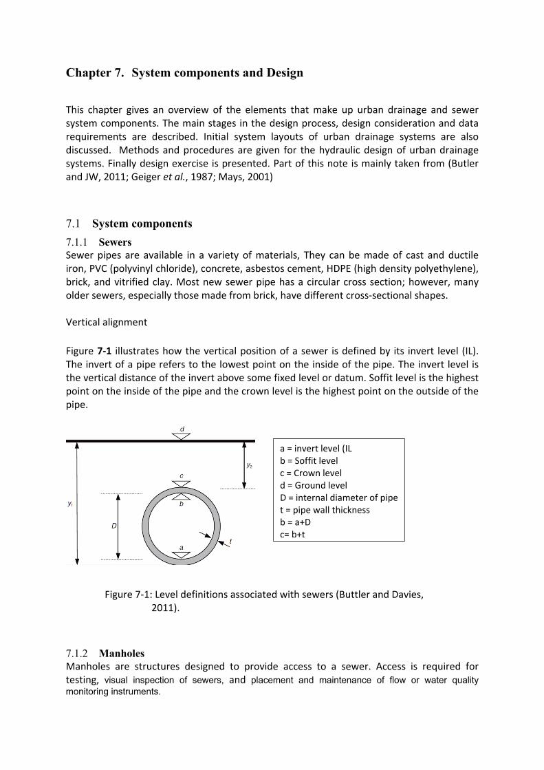
7.1 System components 7.1.1 Sewers Sewer pipes are available in a variety of materials, They can be made of cast and ductile iron, PVC (polyvinyl chloride), concrete, asbestos cement, HDPE (high density polyethylene), brick, and vitrified clay. Most new sewer pipe has a circular cross section; however, many older sewers, especially those made from brick, have different cross-sectional shapes. Vertical alignment Figure 7-1 illustrates how the vertical position of a sewer is defined by its invert level (IL). The invert of a pipe refers to the lowest point on the inside of the pipe. The invert level is the vertical distance of the invert above some fixed level or datum. Soffit level is the highest point on the inside of the pipe and the crown level is the highest point on the outside of the pipe.

Figure 7-1: Level definitions associated with sewers (Buttler and Davies, 2011).

7.1.2 Manholes Manholes are structures designed to provide access to a sewer. Access is required for testing, visual inspection of sewers, and placement and maintenance of flow or water quality monitoring instruments.

a = invert level (IL b = Soffit level c = Crown level d = Ground level D = internal diameter of pipe t = pipe wall thickness b = a+D c= b+t

Manholes are usually provided at heads of runs, at locations where there is changes in direction, changes in gradient; changes in size, at major junctions with other sewers and at every 90 to 200 meter intervals depending on the size of the sewer pipes. The diameter of the manhole will depend on the size of sewer and the orientation and number of inlets.

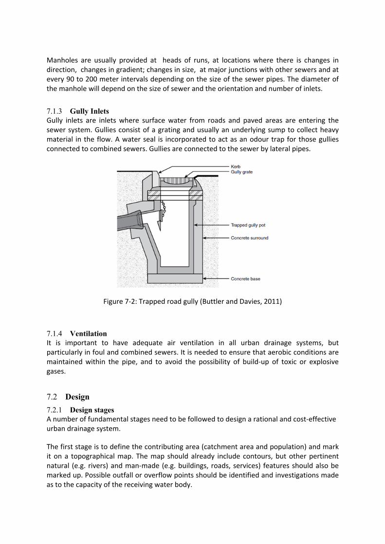
7.1.3 Gully Inlets Gully inlets are inlets where surface water from roads and paved areas are entering the sewer system. Gullies consist of a grating and usually an underlying sump to collect heavy material in the flow. A water seal is incorporated to act as an odour trap for those gullies connected to combined sewers. Gullies are connected to the sewer by lateral pipes.

Figure 7-2: Trapped road gully (Buttler and Davies, 2011)

7.1.4 Ventilation It is important to have adequate air ventilation in all urban drainage systems, but particularly in foul and combined sewers. It is needed to ensure that aerobic conditions are maintained within the pipe, and to avoid the possibility of build-up of toxic or explosive gases.

7.2 Design 7.2.1 Design stages A number of fundamental stages need to be followed to design a rational and cost-effective urban drainage system. The first stage is to define the contributing area (catchment area and population) and mark it on a topographical map. The map should already include contours, but other pertinent natural (e.g. rivers) and man-made (e.g. buildings, roads, services) features should also be marked up. Possible outfall or overflow points should be identified and investigations made as to the capacity of the receiving water body.

The next stage is to produce a preliminary horizontal alignment aiming to achieve a balance between the requirement to drain the whole contributing area and the need to minimise pipe run lengths. Least-cost designs tend to result when the pipe network broadly follows the natural drainage patterns and is branched, converging to a single major outfall. Having located the pipes horizontally, the pipe sizes and gradients can now be calculated based on estimated flows from the contributing area. Generally, sewers should follow the slope of the ground as far as possible to minimise excavation. However, gradients flatter than 1:500 should be avoided as they are difficult to construct accurately. A preliminary vertical alignment can then be produced, again bearing in mind the balance between coverage of the area and depths of pipes. The alignment can be plotted on longitudinal profiles. Pumping should be avoided, particularly on storm sewer systems, but will be needed if excavations exceed about 10m. The final stage involves revising both the horizontal and vertical alignment to minimise cost by reducing pipe lengths, sizes and depths whilst meeting the hydraulic design criteria. Longer sewer runs may be cost-effective if shorter runs would require costlier excavation and/or pumping. Various stages of urban drainage design procedure Stage 1. Data collection and analysis

• Identify the area(s) to be served. • Collect regulatory codes and design guidelines and set system design criteria. • Collect topographic map, geologic and geographic data. • Add location and level of existing or proposed details such as:

o Contours o physical features (e.g. rivers) o road layout o buildings o sewers and other services o outfall point (e.g. near lowest point, next to receiving water body). o Railroads, o Industry and other utilities

• Undertake field investigations, including feature surveys and ground truthing at sites that potentially conflict with other services.

• Identify the natural drainages, streets, and existing or planned wastewater inflow points at the boundaries of the area to be sewered. Locate all proposed sources of wastewater. Identify likely elevations of customer laterals.

Stage 2. Preliminary horizontal layout

• Design the horizontal layout of the sewer, including manholes and possible pumping station locations. If necessary, prepare alternate layouts.

Stage 3. Preliminary sewer sizing • Divide the total area into logical subareas, as needed, and develop design flow rates

for each section in the system.

• Select pipe sizes, slopes, and inverts. Perform the hydraulic design of the system. Revise selections until the design criteria are met.

• Draw preliminary longitudinal profiles (vertical alignment): o ensure pipes are deep enough so all users can connect into the system o try to locate pipes parallel to the ground surface o ensure pipes arrive above outfall level o avoid pumping if possible

Stage 4. Cost estimate

• Complete cost estimate(s) for the design and alternate designs. • Carefully review all designs, along with assumptions, alternates, and costs.

Stage 5. Revise design

• Modify the design or develop alternate designs, or even alternate layouts. This cycles the designer back to the appropriate earlier step.

• Complete the plan and profile construction drawings and prepare the specifications and other bid documents.

7.2.2 Initial Planning Before a new drainage sewer system is designed, an initial planning study should be carried out to address the issues of whether to provide drainage service, the type of conveyance wanted (gravity and/or pressure), and the pros and cons of different types of systems (separate, combined, vacuum, simplified systems). Some of the factors that must be analyzed when considering the construction of a wastewater collection system for example are:

• Population growth and housing density • Suitability to on-site disposal systems • Environmental impact • Pollution problems in the area • Accessibility to and cost of collection systems and sewage treatment • Regulatory requirements • Ease of construction, including the extent of rock excavation required.

An onsite wastewater treatment system that is properly designed, constructed, operated, and maintained and that has a suitable effluent-receiving body may be an appropriate means of wastewater disposal, especially when a development is far from a regional system. However, wastewater collection and centralized treatment systems usually prove to be the most cost-effective solution to providing sewage services. Public health authorities generally favour collection and centralized treatment systems over on-site systems because they are much easier to inspect, monitor, and regulate. A preliminary investigation is generally conducted to determine the potential area to be served, the consequences of not serving the area, how the area will be served, and the economic feasibility of such a project. There is usually some break-even population above which a centralized sewage collection and

treatment system is desirable, although the exact break-even point varies widely, according to site-specific considerations.

7.2.3 Types of Conveyance Sewer systems use gravity, pressure, vacuum, or some combination of these methods to convey wastewater. In most cases, lower total life-cycle costs (construction, operation, and maintenance) favor gravity sewers over pressure or vacuum systems. In gravity systems, pumping may be required to move flows in areas of flat or uneven topography. In these systems, sewage flows by gravity into a wet well and is pumped through a force main.

Low-pressure sewers differ from force mains in that the pumps are located on the property of each customer. These systems are used either where direct gravity flow is not possible or where excavation depths, extensive shallow rock, obstacles, and alignments make the smaller and shallower pressure lines more economical. The pressurized lines may discharge into a wet well or into a gravity sewer.

Vacuum systems operate on the basis of differential air pressure created by a central vacuum station. Wastewater from each connection is discharged to a sump that is isolated from the main line by a valve. When the level in the sump reaches a designated limit, an actuator opens the valve and the vacuum propels the wastewater to the central vacuum station. In a good vacuum system, the maximum water-level differential in each vacuum zone is about 7.6 m. This means that vacuum systems are relegated to rather flat areas. Multiple vacuum zones may be placed in series, but operating complexity and costs increase rapidly

7.2.4 Separate versus Combined Systems In the past, conveyance of sanitary flows and storm drainage in the same conduits (combined sewers) made economic sense. Today, with expensive mandatory treatment requirements in place, the cost of control and treatment for new systems is almost always lower if the two types of flow are conveyed and treated in completely separate sewer systems. Currently, most pollution control agencies specifically prohibit combining storm drainage and wastewaters in their regulations governing new sanitary sewer design, construction, and operation. However, it is conceivable that future treatment requirements for storm waters in urban and industrial settings may become so stringent that combined system conveyance and treatment may again be the more economical solution. The practice of integrated catchment management, which considers the combined effect on receiving waters of stormwater and treated wastewater, may result in some portion (such as the first flush) of stormwater being directed into the sanitary system.

7.2.5 Preliminary Design Considerations Design codes and criteria are promulgated by various public environmental and pollution-control agencies. Codes give information on location and clearances relative to other utilities, flow-generation rates, peaking factors, and hydraulic guidelines. Codes may reflect the effects of local conditions, such as soil and weather, on the design of sewers. Current codes tend to make more use of such terms as “recommended” or “guidelines,” rather than “required” or “mandatory.” Some regulatory agencies have adopted a more performance-based approach to establish system regulations. Design engineers need to be well-versed in these codes.

Depending on the regulatory agency evaluating the design, either the sewers must be able to carry the design flow while flowing full or at some given fraction of the full depth, or the design flow must be some percentage of the full-pipe capacity (e.g., 75 percent of capacity at design flow). The engineer must determine which is the better approach for a given case, as the two requirements can produce different pipe sizes. Minimum slopes to prevent sedimentation and minimum cover to prevent traffic impacts must also be considered.

Where local codes do not exist or do not address a specific issue, widely adopted standards, should be consulted.

In addition to technical design criteria and the hydraulic loads, other pertinent considerations include

the following:

• Costs – The planning, design, construction, operation, and maintenance costs should all be considered in assessing the long-term sustainability of the project.

• Schedule – The time between the initial planning and the operation of a sewer may be as long as a decade, and the project may need to be constructed in phases.

• Operation and maintenance – Gravity sewers are not maintenance free. They require periodic inspections and cleaning, and some components may require repair or replacement. An organization to operate the system must be in place.

• Environment – Construction of the sewer results in both temporary disruption of and long-term effects on the environment. Short-term effects include temporary lowering of the groundwater table and release of sediments. Over its design life, the sewer system will affect the performance of the wastewater treatment facility and the water quality of the receiving water body.

• Regulatory compliance – The sewer project must comply with all applicable laws and regulations. The design criteria should be developed in consultation with the sewer utility and the financing and regulatory agencies. Consensus on the design criteria before the start of the design is essential.

7.2.6 Data Requirements Additional physical data, beyond that necessary for hydraulic analysis, is required for the design of new sewers. The following list of data requirements has been adapted from American Society of Civil Engineers (1982):

• Topography, surface and subsurface conditions, underground utilities and structures, subsoil conditions, water table elevations, traffic control needs, and elevations of structure basements or connection points

• Locations of streets, alleys, or unusual structures; required rights of way; and similar data necessary to define the physical features of a proposed sanitary sewer project, including preliminary horizontal and vertical alignment

• Details of existing sewers to which a proposed sewer may connect • Information pertinent to possible future expansion of the proposed project • Locations of historical and archeological sites, significant plant or animal

communities, or other environmentally sensitive areas.

The data may be obtained from a variety of sources. Maps, aerial photographs, construction drawings, and ground surveys may be queried. Typically, no single data source is complete, so one must identify inconsistencies and fill in gaps. Instrument surveys are the most accurate method of obtaining high quality spatial data. Many vertical-elevation reference and control points should be established systematically along the route.

7.2.7 Alternatives Alternate system configurations, alignments, and pipe sizes must be explored during the design of new sewers. Each alternate design should be considered until it is apparent that it is infeasible or inferior to another design. The point at which an alternative is dropped from consideration will vary. In some cases, a simple calculation will show that an alternative does not meet one or more design criteria. In other cases, an alternative design must be completed, with a detailed cost estimate, before its economic ranking is known.

It may be necessary to document alternate designs dropped from consideration and the reasons for those decisions. Such decisions are made at various levels. The design engineer will typically make decisions regarding pipe sizes, invert elevations, and manhole details. However, decisions regarding alignments, stream crossings, and locations of pump stations often require input from sewer utility management and permitting authorities.

Hydraulic sewer models are invaluable for managing design alternatives. Most modelling packages have capabilities that facilitate the analysis of multiple alternatives without building separate models. A final design report usually should include results of alternate designs that were considered and the justifications for rejecting them.

7.2.8 Initial System Layout Sewers are almost always laid out in a dendritic (treelike) pattern. Unlike water distribution systems, which have pressurized flow in all directions, gravity sewers normally allow flow in only one direction and are rarely looped. Some of the significant factors that affect the layout of the final wastewater collection network are political jurisdictions and boundaries, alignment of existing sewers, land topography, and geology. When new sewers are proposed for an existing development, the locations of all underground utilities should be determined before beginning the layout of the sewage collection system.

Generally speaking, it is most economical to plan the network and design pipes for the service and flows expected at full buildout of the drainage areas. However, the cost of such piping in areas that remain sparsely populated can be significant, and much of the loading may not be realized for many years. This results in tradeoffs between budget limitations and the desire to provide ultimate capacity.

The layout of a gravity sewer system begins with a topographic map of the service area. The drainage divide lines and natural drainage paths for a new service area should be drawn on the map. Then, the locations of the sewer outlet(s) and elevations of the highest services should be identified. The highest manhole is located where it can provide a connection to a lateral from the highest service. The highest possible invert is determined either from the elevation of the basement (or lowest plumbing fixture) minus an adequate drop along the lateral, or the minimum depth that would give a lower elevation.

The sewer should continue along streets or other public rights-of-way at the flattest acceptable slope, as determined by capacity needs, self-cleansing requirements, minimum depth, or service lateral depths.

When localized high points in the sewer alignment are encountered, a downhill slope may be maintained by either deeper excavation or an alternate path. Crossing depressions of streams may require an inverted siphon. Ultimately, the line ends at a connection to a trunk sewer, a wastewater treatment facility, or a pumping station. Sometimes service areas include drainage divides, such that only part of the development can flow by gravity into downstream sewers. Other parts drain by gravity to a pump station that either lifts the flow to the minimum elevation necessary to continue by gravity or pushes the flow through a force main (pressure pipe) to the desired location.

Manhole Location and Spacing Manholes are generally placed at every change in slope, pipe size, or alignment; where two or more incoming lines are joined; at the upstream end of lines; and at distances not greater than about 90 m for diameters less than 150 mm, about 120 m for diameters of 150–400 mm, and about 150 m for diameters of 450 mm or greater. These distances are dictated by regulations and by the reach of cleaning and maintenance equipment. The following are some additional considerations related to manhole location:

• Street intersections are common locations for manholes • A terminal manhole should be located at the upper end of a sanitary sewer to

provide access for maintenance. • Manholes should not be placed in a location that allows surface water to enter.

Location of Pumping Facilities Pumping facilities are logically placed at low points to collect gravity flow from an area and pump it to a desired point. Pumping facilities are best placed on public land, where they are readily accessible but also as isolated as possible to minimize odour and noise complaints.

Aesthetic or other local considerations may require putting a pumping station some distance from the ideal location as determined from an initial hydraulic and cost-efficiency point of view.

Horizontal and Vertical Alignment Once sewer system layouts and design flows have been determined, the engineer can proceed with designing the vertical sewer alignment and sizing the pipes.

Pipe Slopes A minimum velocity must be maintained to prevent solids build-up during low flows and is determined by the tractive force method. Alternatively, the minimum slopes may be used. These minimum slopes vary according to pipe diameter. Usually it is recommended that flow velocities be less than 3m/s at peak flow. Higher velocities may be tolerated if proper consideration is given to the pipe material, abrasive characteristics of the wastewater, turbulence, and thrust at changes in direction. Minimum slopes for house connections are often specified in local codes. In addition to the real need for somewhat steeper slopes for self-cleansing given the small flow rates in most laterals, the steeper minimum slopes cover a multitude of shortcomings commonly encountered with laterals, such as poor slope control, alignment, bedding, placement, and backfill, leading to pipe differential settlement and joint separation.

Curved Sewer Alignment Typically, sewer piping is installed in straight segments, with changes in the vertical or horizontal alignment occurring at manholes. However, in some cases, a good solution may be to use a curved sewer alignment to change direction. For example, a vertically curved alignment might be used to maintain a reasonable depth without the need for additional manholes where the ground surface makes a fairly large change in slope a short distance. A horizontal or vertical curve may be used to avoid obstructions or give future access for lateral connections or repair. Hydraulically, there is little to prohibit curved alignment as long as the minimum slope meets capacity and self-cleansing needs. The main objections to curved alignment are the extra effort and cost for field survey staking and construction, as well as the extra location information needed to avoid damage during future digging, connect laterals, or provide maintenance. When the cost savings resulting from fewer manholes and shallower construction outweighs these problems, curved sewers should be considered.

Minimum Depth of Cover Sewer pipe should be placed as shallow as possible while still being located

• Deep enough to provide gravity service whenever feasible • Below the frost line (in permafrost areas, the sewer must be insulated, perhaps even

heated)

• A reasonable distance below other utilities, especially potable water lines, unless special features are used to protect against contamination

• Deep enough to adequately distribute traffic and other moving surface loads without causing loading stress breaks in pipes or connections

The cover depth is the distance from the soil surface to the top of the outside surface of the pipe. Minimum cover in nontrafficked areas is generally 0.45–0.6 m and in trafficked areas is 1.2–1.5m, depending on the pipe type. In areas with basements needing gravity sewer service, minimum depths have traditionally been 2.4–2.7 m. Modern basements are often used as living areas and may be several feet deeper than they were in the past. Sewers serving these deeper basements may need to be 3.4–3.7 m deep or more. Utilities may have a specification such as “top of sewer must be at least 1 m below basement floor,” although requiring a service line slope of 1 to 2 percent may be a more appropriate way of specifying minimum depth. If very few buildings have significantly deeper basements, individual or local-area pumps that discharge to the street sewer might be a more economical lifecycle solution. A significant cost issue relative to minimum depth sometimes occurs in relatively flat service areas, where the required pipe slope is greater than the slope of the ground surface. As the gravity sewer proceeds downstream, it is forced deeper. An alternative approach, especially where the water table is high or shallow rock is encountered, is to raise the upstream end of the sewer and service buildings with pumps. In such cases, the cost of pumped lateral services on the upstream end should be weighed against the increased construction cost of the deeper system. A rough approximation of the costs of raising the upstream end of a sewer can be made by multiplying the difference in depth by the incremental estimated excavation and pipe placement cost, adding the incremental cost of manholes in the deeper alternative, and comparing this value with the construction and operation costs of the pressurized service line. Maximum Depth Maximum sewer depths are often set at 6–8 m. Common factors that have historically limited depth are as follows:

• Groundwater makes construction more expensive and hazardous, and makes high-quality pipe bedding and pipe placement more difficult.

• Soil layers, rock layers, or other subsurface conditions make excavation very difficult, the cave-in hazard high, or pipe structural loadings too high.

• Trench stability is more difficult to manage with greater depth. Often extreme (costly) measures are needed for deep sewers, such as special cutoff walls and piling support walls.

• Maximum depth capability of excavation and other maintenance equipment available to the owner may be exceeded.

A limitation on maximum depth can be viewed primarily as a cost issue, to be weighed against the cost of increased pumping or alternative horizontal alignment. Since the cost of pumping, including construction and O&M, is very high, even deep sewer placement may cost less than additional pumping stations.

In areas where few or no service laterals are needed, trenchless sewer construction using horizontal directional drilling or boring and jacking may prove cost effective. Trenchless construction can also be used (and is often required) for service laterals where they cross railroads, streams, or major highways. Special Installations Sewers must sometimes be installed in steep terrain or along or across streams or other obstructions. The subsections that follow describe some special installation types. Sewers in Steep Terrain If steep terrain results in velocities in excess of 4.6 m/s, the engineer should consider using more durable pipe materials such as ductile iron and an energy-dissipation manhole at the end of the steep slope. Alternatively, flatter slopes can be maintained through the use of drop manholes. With a drop manhole configuration, pipes are commonly sloped to prevent velocities in excess of approximately 3 m/s. The water drop in the manhole dissipates energy without causing extremely high velocities, which are both a hazard to workers in the manhole and abrasive to the pipes. However, drop manholes do cause turbulence, which can release hydrogen sulfide from the wastewater, resulting in odor and corrosion problems. Sewers along Streams When sewers must be routed along waterways, extra care is needed to protect the sewer from erosion and breakage. Sewers placed parallel to streams or drainage channels are typically constructed of lined ductile iron or plastic pipe. The sewer is normally still designed as an open-channel flow conduit, but an inverted siphon may be required when crossing under a waterway. If the probability of breakage and spills is deemed significant, the streambank may need to be stabilized to prevent washout of the pipe. Stabilization is preferably achieved using a method based on the stream’s natural geomorphology. Elevated Crossings Sometimes the best solution to crossing an obstruction such as a canal, stream, or gully is to use an elevated, above-grade structure. In some cases, open-channel flow can be maintained. If the flow must be pressurized at the crossing (i.e., there is a sag in the pipe), then it is an inverted siphon. A true elevated sewer will have the same slope as the upstream and downstream pipes. The designer should examine the ground profile to identify the segment of pipe that is above grade. Special pipe materials and construction techniques may be required for the exposed pipe. For example, some plastic pipes may be damaged by ultraviolet light, while metal pipe may need a wrap or coating. Inverted Siphons (Depressed Sewers) An inverted siphon is a sag in a sewer used to avoid an obstruction such as a gulley, stream, canal, depressed railway, or roadway. However, this type of structure is not really a siphon, and the term depressed sewer has been suggested as more appropriate. Because the pipe(s) comprising the inverted siphon are below the hydraulic grade line, it always contains sewage, and its hydraulic behaviour is that of a pressure-flow conduit. Minimum diameters for depressed sewers are the same as for gravity sewers: 150 or 200 mm. Depressed sewers require a larger sediment carrying capacity for self-cleansing than do normal, open-channel sewers, because it is desirable to scour larger particles out of the

siphon to avoid build-up and clogging, and also because particles must be suspended in the turbulent flow to be successfully removed. To make them as maintenance free as possible, velocities of at least 0.9 m/s need to be achieved at a minimum of every few days. Higher velocities can be induced by placing a splitter box with different weir levels at the inlet and using two or more parallel pipes in the siphon section. All flow goes into the smaller pipe until it surcharges, then the overflow spills into the next pipe, and so on. Depressed sewers are usually constructed using lined ductile iron or plastic pressure pipe. The hydraulic design is best handled by applying the energy equation from the inflow section at the entrance to the depressed section, through the transitions (bends), to the outlet where flow enters the open-channel pipe. Head loss resulting from changes in velocity at the entrance must be accounted for.

7.2.9 Hydraulic Design Storm drainage networks physically connect stormwater inlet points such as road gullies and roof downpipes to a discharge point or outfall, by a series of continuous and unbroken pipes. Flow into the sewer results from the random input over time and space of rainfall-runoff. Generally, these flows are intermittent, of relatively long duration and are hydraulically unsteady. Separate storm sewers will stand empty for long periods of time. The extent to which the capacity is taken up during rainfall depends on the magnitude of the event and conditions in the catchment. During low rainfall, flows will be well below the available capacity, but during very high rainfall the flow may exceed the pipe capacity inducing pressure flow and even surface flooding. Design is accomplished by first choosing a suitable design storm. The physical properties of the storm contributing area must then be quantified. A number of methods of varying degrees of sophistication have been developed to estimate the runoff flows resulting from rainfall. The concepts of statistically analysed rainfall and the design storm give statistically representative rainfall that can be applied to the contributing area and converted into runoff flows. Once flows are known, suitable pipes can be designed. The choice of design storm return period therefore determines the degree of protection from stormwater flooding provided by the system. This protection should be related to the cost of any damage or disruption that might be caused by flooding. In practice, cost–benefit studies are rarely conducted for ordinary urban drainage projects, a decision on design storm return period is made simply on the basis of judgement and precedent. Although we can assess and specify design rainfall return period, our greatest interest is really in the return period of flooding. It is normally assumed that the frequency of rainfall is equivalent to the frequency of runoff. However, this is not completely accurate. For example, antecedent soil moisture conditions, areal distribution of the rainfall over the catchment and movement of rain all influence the generation of stormwater runoff. These conditions are not the same for all rainfall events, so rainfall frequency cannot be identical to runoff frequency. However, comprehensive storm runoff data is less common than rainfall records, and so the assumption is usually the best reasonable approach available.

Urban drainage systems deal with both wastewater and stormwater. Most stormwater is the result of rainfall. Other forms of precipitation – snow for example – are contributors too, but rainfall is by far the most significant in most places. Methods of representing and predicting rainfall are therefore crucial in the design, analysis and operation of drainage systems. Rainfall Analysis

Rain data measured at an individual rain gauge is most commonly expressed either as depth in mm or intensity in mm/h. This type of point rainfall data is therefore representative of one particular location on the catchment. Such data is of greater value if it can be related statistically to two other important rainfall variables: duration and frequency (or probability). The rainfall duration refers to the time period D minutes over which the rainfall falls. However, duration is not necessarily the time period for the whole storm, as any event can be subdivided and analysed for a range of durations. It is common to represent the frequency or probability of the rainfall as a return period. An annual maximum rainfall event has a return period of T years if it is equalled or exceeded in magnitude once, on average, every T years. Thus a rainfall event that occurs on average twenty times in 100 years has a probability of being equalled or exceeded of 0.2, and a return period of 5 years. Annual maximum storm events are normally used to determine return period because it is assumed that the largest event in one year is statistically independent of the largest event in any other year. IDF relationships Definition A convenient form of rainfall information is the intensity-duration-frequency (IDF) relationship. For an event with a particular return period, rainfall intensity and duration are inversely related. As the duration increases, the intensity reduces. This confirms the common-sense observation that heavy storms only last a short time, but drizzle can go on for long periods. Also, frequency and intensity are related, as rarer events (greater return periods) tend to have higher intensities (for a given duration). Derivation When local rainfall data are available, IDF curves can be developed using frequency analysis Steps for IDF analysis are:

1. The IDF analysis starts by gathering time series records of different duration. ( eg. 5, 10, 15, 20, 30, 60, 90, and 120 min).

2. After time series data is gathered, annual extremes are extracted from the record of each duration.

3. The annual extreme data is then fit to a probability distribution in order to estimate rainfall quantities.

T TX K

where

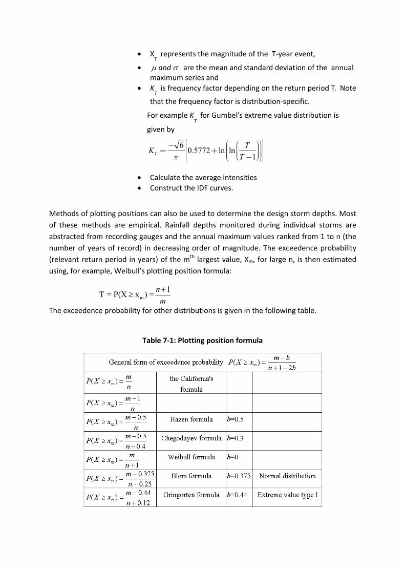
• XT represents the magnitude of the T-year event,

• µ and σ are the mean and standard deviation of the annual maximum series and

• KT is frequency factor depending on the return period T. Note

that the frequency factor is distribution-specific.

For example KT for Gumbel’s extreme value distribution is

given by

6 0.5772 ln ln1T

TKT

• Calculate the average intensities • Construct the IDF curves.

Methods of plotting positions can also be used to determine the design storm depths. Most of these methods are empirical. Rainfall depths monitored during individual storms are abstracted from recording gauges and the annual maximum values ranked from 1 to n (the number of years of record) in decreasing order of magnitude. The exceedence probability (relevant return period in years) of the mth largest value, Xm, for large n, is then estimated using, for example, Weibull’s plotting position formula:

m1T = P(X x ) = n

m+

≥

The exceedence probability for other distributions is given in the following table.

Table 7-1: Plotting position formula

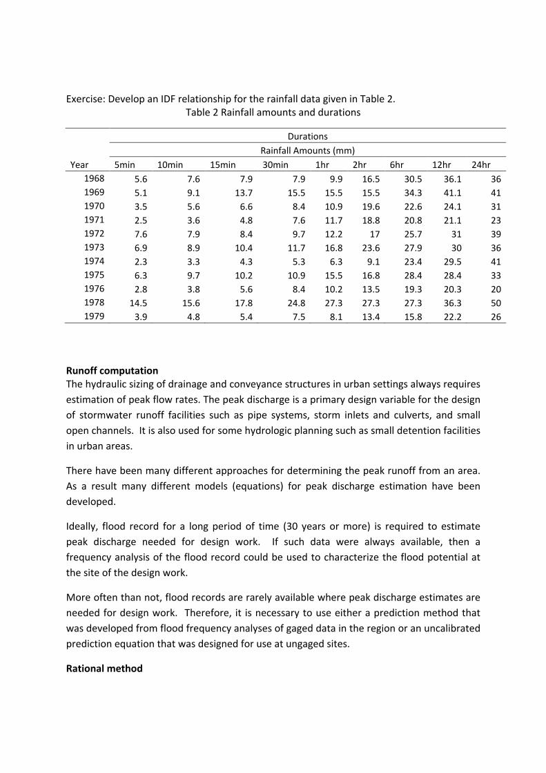
Exercise: Develop an IDF relationship for the rainfall data given in Table 2.

Table 2 Rainfall amounts and durations

Year

Durations Rainfall Amounts (mm)

5min 10min 15min 30min 1hr 2hr 6hr 12hr 24hr 1968 5.6 7.6 7.9 7.9 9.9 16.5 30.5 36.1 36 1969 5.1 9.1 13.7 15.5 15.5 15.5 34.3 41.1 41 1970 3.5 5.6 6.6 8.4 10.9 19.6 22.6 24.1 31 1971 2.5 3.6 4.8 7.6 11.7 18.8 20.8 21.1 23 1972 7.6 7.9 8.4 9.7 12.2 17 25.7 31 39 1973 6.9 8.9 10.4 11.7 16.8 23.6 27.9 30 36 1974 2.3 3.3 4.3 5.3 6.3 9.1 23.4 29.5 41 1975 6.3 9.7 10.2 10.9 15.5 16.8 28.4 28.4 33 1976 2.8 3.8 5.6 8.4 10.2 13.5 19.3 20.3 20 1978 14.5 15.6 17.8 24.8 27.3 27.3 27.3 36.3 50 1979 3.9 4.8 5.4 7.5 8.1 13.4 15.8 22.2 26

Runoff computation The hydraulic sizing of drainage and conveyance structures in urban settings always requires estimation of peak flow rates. The peak discharge is a primary design variable for the design of stormwater runoff facilities such as pipe systems, storm inlets and culverts, and small open channels. It is also used for some hydrologic planning such as small detention facilities in urban areas.

There have been many different approaches for determining the peak runoff from an area. As a result many different models (equations) for peak discharge estimation have been developed.

Ideally, flood record for a long period of time (30 years or more) is required to estimate peak discharge needed for design work. If such data were always available, then a frequency analysis of the flood record could be used to characterize the flood potential at the site of the design work.

More often than not, flood records are rarely available where peak discharge estimates are needed for design work. Therefore, it is necessary to use either a prediction method that was developed from flood frequency analyses of gaged data in the region or an uncalibrated prediction equation that was designed for use at ungaged sites.

Rational method

Historically, ‘‘Rational method’’ has been the tool of choice for most practicing engineers around the world. Although the method definitely has its place in hydrologic design, it is routinely misapplied and overextended.

The concept is attractive and easy to understand. If rainfall occurs over a basin at a constant intensity for a period of time that is sufficient to produce steady state runoff at the outlet or design point, then the peak outflow rate will be proportional to the product of rainfall intensity and basin area. Mathematically, the rational method relates the peak discharge (q, m3/sec) to the drainage area (A, ha), the rainfall intensity (i, mm/hr), and the runoff coefficient (C). In SI units the rational formula is given as;

q = CiA/360

where q = design peak runoff rate in m3/s C = the runoff coefficient

i = rainfall intensity in mm/h for the design return period and for a duration equal to the “time of concentration” of the catchment.

Assumption of the rational method

• The rate of runoff resulting from any constant rainfall intensity is maximum when the

duration of rainfall equals the time of concentration. That is, if the rainfall intensity is

constant, the entire drainage area contributes to the peak discharge when the time of

concentration has elapsed.

• The frequency of peak discharge is the same as the frequency of the rainfall intensity for

the given time of concentration.

• The rainfall intensity is uniformly distributed over the entire drainage area.

• The fraction (C) of rainfall that becomes runoff is independent of rainfall intensity or

volume.

Limitation of the rational method

• For large drainage areas, the time of concentration can be so large that the assumption of

constant rainfall intensities for such long periods is not valid, and shorter more intense

rainfalls can produce larger peak flows. Additionally, rainfall intensities usually vary during

a storm. In semi-arid and arid regions, storm cells are relatively small with extreme

intensity variations.

• Frequencies of peak discharges depend on rainfall frequencies, antecedent moisture

conditions in the catchment and the response characteristics of the drainage system.

• For small, mostly impervious areas, rainfall frequency is the dominant factor. For larger

drainage basins, the response characteristics are the primary influence on frequency. For

drainage areas with few impervious surfaces (less urban development), antecedent

moisture conditions usually govern, especially for rainfall events with a return period of 10

years or less.

• In reality, rainfall intensity varies spatially and temporally during a storm. For small areas,

the assumption of uniform distribution is reasonable. However, as the drainage area

increases, it becomes more likely that the rainfall intensity will vary significantly both in

space and time.

• The constant runoff coefficient assumption is reasonable for impervious areas, such as

streets, rooftops, and parking lots. For pervious areas, the fraction of runoff varies with

rainfall intensity, accumulated volume of rainfall, and antecedent moisture conditions.

Thus, the art necessary for application of the Rational Method involves the selection of a

coefficient that is appropriate for storm, soil, and land use. By limiting the application of the

Rational Method to 80 hectares, these assumptions are more likely to be reasonable.

• Modern drainage practice often includes detention of urban storm runoff to reduce the peak

rate of runoff downstream and to provide storm water quality improvement. The Rational

Method severely limits the evaluation of design alternatives available in urban and, in some

instances, rural drainage design because of its inability to accommodate the presence of

storage in the drainage area.

Application of the rational method Taking in to account the various assumptions and limitations in the application of the rational

method, the method is applicable in estimating storm water runoff peak flows for the design of

hydraulic designs on very small catchments, design of gutter flows, drainage inlets, storm drain

pipes, culverts and small ditches. It is most applicable to small, highly impervious areas. It is worthy

of nothing that the method is applied to small areas to guarantee homogeneity and should not be

used for calculating peak flows downstream of major hydraulic structures like bridges, culverts and

storm sewers that may act as a restrictions and impact the rate of discharge

Description of the Rational Method input variables Runoff Coefficient C It is a dimensionless ratio intended to indicate the amount of runoff

generated by a catchment given an average intensity of precipitation for a storm. This variable

represents the ratio of runoff to rainfall. It is the most difficult input variable to estimate. It

represents the interaction of many complex factors, including the storage of water in surface

depressions, infiltration, antecedent moisture, ground cover, ground slopes, and soil types. In

reality, the coefficient may vary with respect to prior wetting and seasonal conditions. The use of

average values has been adopted to simplify the determination of this coefficient. Where a

drainage area is composed of subareas with different runoff coefficients, a composite coefficient for

the total drainage area is computed by dividing the summation of the products of the subareas and

their coefficients by the total area.

Table 3 Runoff Coefficients for Urban Areas

(from Storm Water Systems design handbook)

Type of drainage area Runoff coefficient Business: Downtown areas 0.70–0.95

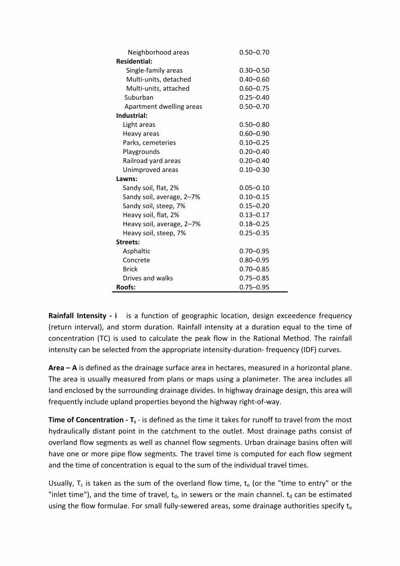
Neighborhood areas 0.50–0.70 Residential: Single-family areas 0.30–0.50 Multi-units, detached 0.40–0.60 Multi-units, attached 0.60–0.75 Suburban 0.25–0.40 Apartment dwelling areas 0.50–0.70 Industrial: Light areas 0.50–0.80 Heavy areas 0.60–0.90 Parks, cemeteries 0.10–0.25 Playgrounds 0.20–0.40 Railroad yard areas 0.20–0.40 Unimproved areas 0.10–0.30 Lawns: Sandy soil, flat, 2% 0.05–0.10 Sandy soil, average, 2–7% 0.10–0.15 Sandy soil, steep, 7% 0.15–0.20 Heavy soil, flat, 2% 0.13–0.17 Heavy soil, average, 2–7% 0.18–0.25 Heavy soil, steep, 7% 0.25–0.35 Streets: Asphaltic 0.70–0.95 Concrete 0.80–0.95 Brick 0.70–0.85 Drives and walks 0.75–0.85 Roofs: 0.75–0.95

Rainfall Intensity - i is a function of geographic location, design exceedence frequency (return interval), and storm duration. Rainfall intensity at a duration equal to the time of concentration (TC) is used to calculate the peak flow in the Rational Method. The rainfall intensity can be selected from the appropriate intensity-duration- frequency (IDF) curves.

Area – A is defined as the drainage surface area in hectares, measured in a horizontal plane. The area is usually measured from plans or maps using a planimeter. The area includes all land enclosed by the surrounding drainage divides. In highway drainage design, this area will frequently include upland properties beyond the highway right-of-way.

Time of Concentration - Tc - is defined as the time it takes for runoff to travel from the most hydraulically distant point in the catchment to the outlet. Most drainage paths consist of overland flow segments as well as channel flow segments. Urban drainage basins often will have one or more pipe flow segments. The travel time is computed for each flow segment and the time of concentration is equal to the sum of the individual travel times.

Usually, Tc is taken as the sum of the overland flow time, to (or the "time to entry" or the "inlet time"), and the time of travel, td, in sewers or the main channel. td can be estimated using the flow formulae. For small fully-sewered areas, some drainage authorities specify to

as a constant typically ranging from 5 to 15 minutes. In more complex situations, it is recommended to use the kinematic wave formula in the following form (Geiger et al., 1987):

0.6 0.6 0.4 0.30 6.9t L n i s−=

where to is in minutes, L is the travelled length (m), n is the Manning's roughness coefficient, i is the rain fall intensity (mm/hr), and S is the slope (m/m).

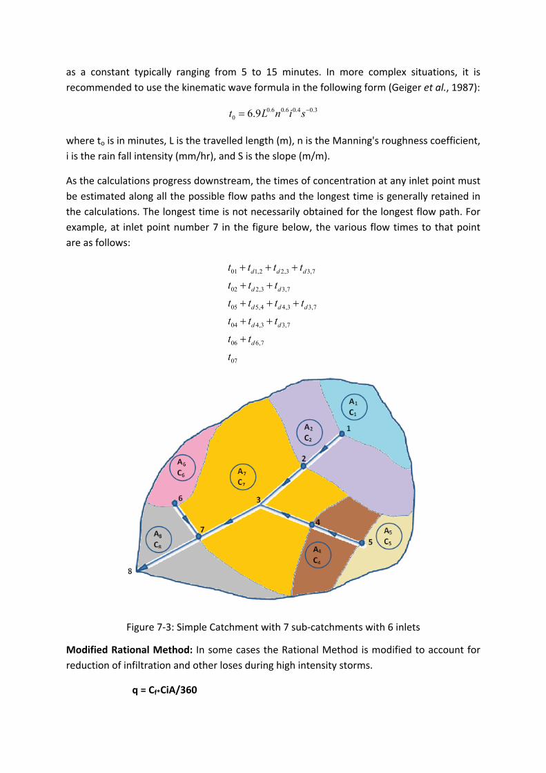
As the calculations progress downstream, the times of concentration at any inlet point must be estimated along all the possible flow paths and the longest time is generally retained in the calculations. The longest time is not necessarily obtained for the longest flow path. For example, at inlet point number 7 in the figure below, the various flow times to that point are as follows:

01 1,2 2,3 3,7

02 2,3 3,7

05 5,4 4,3 3,7

04 4,3 3,7

06 6,7

07

d d d

d d

d d d

d d

d

t t t tt t tt t t tt t tt tt

+ + +

+ +

+ + +

+ +

+

Figure 7-3: Simple Catchment with 7 sub-catchments with 6 inlets

Modified Rational Method: In some cases the Rational Method is modified to account for reduction of infiltration and other loses during high intensity storms.

q = Cf*CiA/360

Less frequent, higher intensity storms require adjusted runoff coefficients because infiltration and other losses have a proportionally smaller effect on runoff. The runoff coefficient are usual applicable for 10 year or less recurrence intervals. Runoff coefficient adjustment factor Cf for storms of different recurrence intervals are listed below.

Table 4 Runoff Coefficient Adjustment Factors

Recurrence interval (years) Runoff coefficient adjustment factor Cf 10 or less 1 25 1.1 50 1.2 100 1.25

Hydrograph methods One of the major weaknesses of the Rational Method is that it only produces worst-case design flow and not a hydrograph of flow against time. Hydrograph methods have been developed to overcome this limitation.

When catchments are large, that is, when they are comprised of two or more smaller catchments whose streamflow at the confluence with common collector channel can be expected to be displaced in time, where storage influences the time distribution of flow in a stream, or where storage is a part of the design problem, peak flow methods are inappropriate for hydrologic design. In these instances, it is necessary to estimate the entire flow hydrograph.

Time–area Method Area is treated as a constant in the Rational Method. In reality, the contributing area is not constant. For example, during the beginning of rainfall the area builds up with time, closest surfaces contributing first, more distant ones later.

The Time–area Method uses the time–area diagram to produce not only a peak design flow, but also a flow hydrograph. The method also allows straightforward use of time-varying rainfall – the design storm.

The Time–area Method utilizes a common, basic approach in determining the hydrograph at the outlet. The cumulative time-area curve is formed by summing the incremental areas and the corresponding travel times. Thus, the total time can be thought of as the time of concentration of the catchment under consideration.

The diagram is used for storm sewer design by assuming that the time–area plot for each individual pipe sub-catchment is linear. However, the design of each pipe is not concerned just with the local sub-catchment but also with the ‘concentrating’ flows from upstream pipes. The combined time–area diagram for each pipe can be produced using the principle

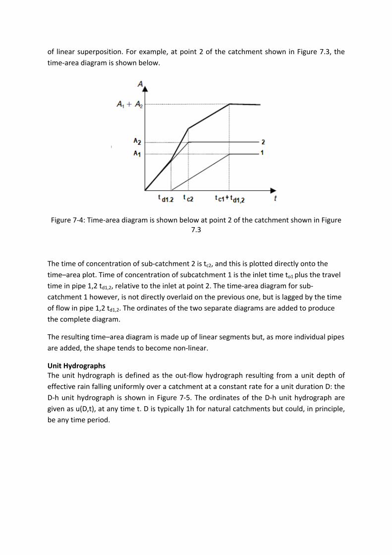
of linear superposition. For example, at point 2 of the catchment shown in Figure 7.3, the time-area diagram is shown below.

Figure 7-4: Time-area diagram is shown below at point 2 of the catchment shown in Figure 7.3

The time of concentration of sub-catchment 2 is tc2, and this is plotted directly onto the time–area plot. Time of concentration of subcatchment 1 is the inlet time to1 plus the travel time in pipe 1,2 td1,2, relative to the inlet at point 2. The time-area diagram for sub-catchment 1 however, is not directly overlaid on the previous one, but is lagged by the time of flow in pipe 1,2 td1,2. The ordinates of the two separate diagrams are added to produce the complete diagram.

The resulting time–area diagram is made up of linear segments but, as more individual pipes are added, the shape tends to become non-linear.

Unit Hydrographs The unit hydrograph is defined as the out-flow hydrograph resulting from a unit depth of effective rain falling uniformly over a catchment at a constant rate for a unit duration D: the D-h unit hydrograph is shown in Figure 7-5. The ordinates of the D-h unit hydrograph are given as u(D,t), at any time t. D is typically 1h for natural catchments but could, in principle, be any time period.

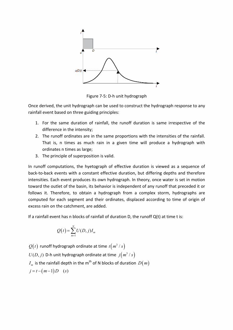
Figure 7-5: D-h unit hydrograph

Once derived, the unit hydrograph can be used to construct the hydrograph response to any rainfall event based on three guiding principles:

1. For the same duration of rainfall, the runoff duration is same irrespective of the difference in the intensity;

2. The runoff ordinates are in the same proportions with the intensities of the rainfall. That is, n times as much rain in a given time will produce a hydrograph with ordinates n times as large;

3. The principle of superposition is valid.

In runoff computations, the hyetograph of effective duration is viewed as a sequence of back-to-back events with a constant effective duration, but differing depths and therefore intensities. Each event produces its own hydrograph. In theory, once water is set in motion toward the outlet of the basin, its behavior is independent of any runoff that preceded it or follows it. Therefore, to obtain a hydrograph from a complex storm, hydrographs are computed for each segment and their ordinates, displaced according to time of origin of excess rain on the catchment, are added.

If a rainfall event has n blocks of rainfall of duration D, the runoff Q(t) at time t is:

( )1

( , )N

mm

Q t U D j I=

=∑

( )Q t runoff hydrograph ordinate at time ( )3 /t m s

( , )U D j D-h unit hydrograph ordinate at time ( )3 /j m s

mI is the rainfall depth in the mth of N blocks of duration ( )D m

( )1 ( )j t m D s= − −

Synthetic unit hydrographs Because of lack of runoff records available for derivation of unit hydrographs from actual rain-runoff events, hydrologic design depends on methods of synthetic hydrograph formulation.

There are a number of different procedures for development of synthetic unit hydrographs. The SCS dimensionless unit hydrograph (1985) is frequently used in the practice.

The dimensionless time and flow rate ordinates are dimensionalized by multiplying the ratios in the columns by tp (in either hours or minutes) and Qp (cumecs), respectively. The result is a tr-hour (or minute) unit hydrograph where tr is the effective duration, calculated as;

0.133*r ct t=

and tc is the time of concentration for the catchment under consideration. Time to peak, tp, is calculated as

0.6*2r

p ctt t= +

The peak flow rate, Qp, is calculated as

2.08*p

p

AQt

=

where A is catchment area in square kilometres

tp is time to peak flow rate, hours

Table 5 SCS Dimensionless Unit Hydrograph

t/tp Q/Qp t/tp Q/Qp 0 0 2.6 0.107

0.2 0.1 2.8 0.077 0.4 0.31 3 0.055 0.6 0.66 3.2 0.04 0.8 0.93 3.4 0.029

1 1 3.6 0.021 1.2 0.93 3.8 0.015 1.4 0.78 4 0.011 1.6 0.56 4.2 0.008 1.8 0.39 4.4 0.006

2 0.28 4.6 0.004 2.2 0.207 4.8 0.002

Once the time to peak tp and peak flow Qp are calculated as above, the SCS dimensionless unit hydrograph is used to calculate the ordinates of the hydrograph

The figure below show a hydrograph produced from hyetograph of excess rain (three different depth of 0.5h duration each). The hyetograph of excess rain is shown inverted over the hydrographs. The depth of excess rain in each segment of the hyetograph is shown. The triangular hydrographs are the hydrographs of excess rain, lagged in time so that the start of the rising limb corresponds in time to the beginning of a new rainfall segment. In the second graph the ordinates of the individual component hydrographs have been added to obtain the design hydrograph

Figure 7-6: Three effective rainfall of o.5hr duration and their resulting hydrographs

Figure 7-7: Design hydrograph resulting from the storm event (the sum of the three hydrographs produce the deign hydrographs shown in broken line)

Flow

rate

Hour

Kinematic wave methods Unit hydrograph methods are empirical approaches to runoff computation that circumvent the necessity of physical representation of the laws of conservation of mass and of momentum that govern the actual movement of water over land surface. The practical reasons for this approach are 1) the various components of runoff generation and movement of runoff are not well understood; and 2) the complexity of the processes is so enormous that it would be impractical to collect all the required data and code them into a computerized computational scheme. However, in some cases (e.g. very small areas, small areas with a high percentage of impervious surface), kinematic wave methods may be preferable to unit hydrograph methods for computing hydrographs of direct runoff.

The kinematic wave approach derives from the one-dimensional continuity and momentum equations (St. Venant equations) that describe the physical processes of the movement of water. The kinematic wave equation results when the inertial terms and the pressure terms have minimal influence on the transmission of water.

The concept of kinematic wave approach for surface runoff computation is based on the kinematic wave computation. This means that the surface runoff is computed as flow in an open channel, taking the gravitational and friction forces only. The runoff amount is controlled by the various hydrological losses and the size of the actually contributing area.

The shape of the runoff hydrograph is controlled by the catchment parameters length, slope and roughness of the catchment surface. These parameters form a base for the kinematic wave computation (Manning equation).

Figure 7-8: The simulated processes in kinematic wave approach for runoff generation

5132* * *t tQ M B S y=

,eff t t t t t tI P E S W I= − − − −

Where tQ = discharge at time t M = Manning’s roughness number B = Flow channel width S = Surface slop

ty = Runoff depth at time t ,eff tI = Effective precipitation

tP = Rainfall depth at time t tE = Evapotranspiration at time t tS = Surface storage loss at time t tW = Wetting loss at time t tI = Infiltration loss at time t

ty is determined from continuity equation

, * *teff t t

dyI A Q Adt

− =

Where A is contributing catchment area

References

Butler, D., and JW, D. (2011), Urban Drainage, Taylor & Francis.

Geiger, W. F., 2.9, I. H. P. W. G.-.-P. A., and Unesco (1987), Manual on Drainage in Urbanized Areas:

Planning and design of drainage systems, Unesco.

Mays, L. W. (2001), Stormwater collection systems design handbook, McGraw-Hill Professional.