system appendPDF cover-forpdf · 12 planning was suggested by Bitran and Hax (1977) as a means to solve a production scheduling 13 problem

Draft

Evaluating a hierarchical approach to landscape level

harvest scheduling

Journal: Canadian Journal of Forest Research

Manuscript ID cjfr-2017-0298.R2

Manuscript Type: Article

Date Submitted by the Author: 01-Dec-2017

Complete List of Authors: Eyvindson, Kyle; University of Jyväskylä, Department of Biological and Environmental Science Rasinm�ki, Jussi; Simosol Kangas, Annika; Natural Resources Institute Finland (Luke), Economics and society

Keyword: Hierarchical planning, landscape level-planning, decision making, strategic planning, tactical planning

Is the invited manuscript for consideration in a Special

Issue? : N/A

https://mc06.manuscriptcentral.com/cjfr-pubs

Canadian Journal of Forest Research

Draft

1

1

2

3

4

5

Evaluating a hierarchical approach to landscape level harvest 6

scheduling 7

Kyle Eyvindson*1, Jussi Rasinmäki2, Annika Kangas3 8

9

10

*1 University of Jyvaskyla, Department of Biological and Environmental Science, P.O. Box 35, 11

40014 University of Jyvaskyla Finland [email protected] 12

13

2 Simosol Oy, Rautatietori 4, 11130 Riihimäki,Finland 14

3 Economics and Society, Natural Resources Institute Finland (Luke), P.O. Box 68, 80101 15

Joensuu, Finland 16

Keywords: Hierarchical planning, landscape-level planning, decision making, strategic planning, 17

tactical planning 18

19

20

21

Page 1 of 34



Draft

2

Abstract 1

The conduct of landscape level forest planning has the potential to become a large intractable 2

problem. In Finland, Metsähallitus (the state enterprise which manages federally owned land) 3

creates strategic plans to determine the appropriate harvest level. While these plans are feasible, 4

they are not implementable in practice as the harvests are scattered temporally and spatially. 5

Requiring that harvests be organized both temporally and spatially for practical implementation 6

can result in an intractable problem. Through a hierarchical approach the problem can be 7

organized into steps, where the intractable problem is broken down into smaller easily solvable 8

parts. As an approximation technique, the hierarchical approach may not find a solution close to 9

optimality. To meet this challenge, we combine the top hierarchical level with a limited selection 10

of lower hierarchical level problems into a single optimization problem. Then an iterative 11

process is used to improve the link between the hierarchical levels. We evaluate the landscape 12

level management plans developed by the iterative approach with a solution to the complete 13

problem. The iterative process dramatically improves the strategic solution, performing near the 14

global optimum. This suggests the process can be applied to more computationally challenging 15

problems, such as spatial planning and stochastic programming. 16

Keywords: Hierarchical planning, landscape level-planning, decision making, strategic 17

planning, tactical planning 18

Page 2 of 34



Draft

3

Introduction 1

Landscape level forest planning is a multi-criteria problem which strives to promote the 2

production of timber resources while either enhancing or preventing ecological and social losses 3

(Kangas et al. 2000). At this level of planning, spatial issues are important for both ecological 4

and economic perspectives. The addition of spatial considerations can dramatically increase the 5

problems computational complexity (Borges et al. 2017). If the complexity of the problem 6

becomes too great, these problems can become intractable. For these cases, simplification of the 7

problem becomes necessary. This process of problem simplification changes the structure of the 8

problem and introduces potential for inefficiencies. These inefficiencies may or may not be 9

meaningful, however if the original problem would become tractable these inefficiencies can be 10

evaluated. 11

12

One approach to solving large scale forest management problems is the use of hierarchical 13

approach to planning. In hierarchical planning, the aim is to solve a combination of smaller 14

problems in a systematic fashion so that each piece of the problem is easily solvable. Often, these 15

approaches can be classified according to which direction in the hierarchy the problems are 16

solved. A top-down approach first solves for the comprehensive problem (i.e. the maximum 17

sustainable yield of the strategic plan) which guides the planning in sub levels (i.e. the tactical 18

planning of specific harvest levels at sub regions). The top-down approach may over-estimate the 19

potential of what is possible for the sublevels. For instance, spatial restrictions and additional 20

constraints (Öhman and Eriksson 2010) may limit the potential to reach the objectives of the top-21

level requirements. Correspondingly a bottom up approach first generates feasible plans for sub 22

regions, and the comprehensive problem is solved using the set of lower level solutions (see Hof 23

Page 3 of 34



Draft

4

and Pickens 1987, Kurttila et al. 2001 and Hiltunen et al. 2012). The performance of the global 1

solution will most likely be sub-optimal, as the development of sub-region plans is a 2

simplification of the overall problem. This restriction in the creation of the sub-region plans 3

simplifies the problems, but limits the potential interaction between hierarchical levels 4

(Weintraub and Cholaky 1991). A hierarchical planning approach can also integrate a top-down 5

and bottom-up approaches. The focus should be on combining the advantages, while limiting the 6

increased cost attributed to the increased complexity of the approach. The potential for 7

integrating both approaches has been suggested in several applications of hierarchical planning 8

(Weintraub and Cholaky 1991; Kurttila et al. 2001; Pittman, Bare and Briggs 2007). 9

10

The use of hierarchical planning approaches has a fairly long history. The process of hierarchical 11

planning was suggested by Bitran and Hax (1977) as a means to solve a production scheduling 12

problem. The first applications of hierarchical planning in forestry used one pass methods to 13

create an appropriate set of solutions for each level (Smith 1978; Hof and Pickens 1987; 14

Weintraub et al. 1986). To improve the hierarchical approach Weintraub and Cholaky (1991) 15

suggested a method to iterate between planning levels as a means to improve the solution quality. 16

This approach was shown through a small wood procurement example. 17

18

In addition to solving computationally difficult problems, hierarchical planning can be applicable 19

when solving problems that are distributed amongst various agents (Scheeweiss 2003). When the 20

local forest managers make decisions in a fairly independent manner, a hierarchical approach 21

may better approximating the actual structural process of how decisions are made. This may be 22

very important for the organisation level decisions (e.g. Hiltunen et al. 2012). 23

Page 4 of 34



Draft

5

1

The implementation of hierarchical planning approach can vary depending on the specific 2

planning case. For instance, hierarchical planning cases can be applied to link temporal scales, 3

linking strategic long-term planning with tactical short-term timber planning requirements 4

(Paradis et al. 2013). The link could be applied to spatial scale, linking holding level spatial 5

scales to regional level spatial scales (Kangas et al. 2014). The hierarchical framework could also 6

be multi-layered, linking both spatial and temporal concerns together. The usefulness of the 7

hierarchical approach is to adjust the problem so that it is solvable, and the resulting plan is 8

implementable. 9

10

The intent of this research is to identify and evaluate an approach for conducting hierarchical 11

forest planning at a landscape level which generates solutions very near the global optimal. This 12

work can be seen as an extension of Kangas et al. (2014), where they developed a hierarchical 13

bottom-up approach for Metsähallitus (the Finnish state forest organization). Their approach to 14

creating the initial bottom-level solutions is modified and extended through the inclusion of 15

iterative approach in creating additional solutions for the bottom-level. To evaluate the 16

hierarchical solutions at each iterative step, we formulate the global problem and solve it using a 17

commercial solver. The results highlight the potential for hierarchical planning in solving large-18

scale problems, and potentially to allow for the inclusion of stochastic elements in the 19

optimization at landscape or regional levels. 20

21

Materials 22

Page 5 of 34



Draft

6

The dataset used for this study has been utilized in two previous studies. The first attempt to 1

solve this landscape level plan was by Virtanen (2010), where she attempted to find a solution 2

which optimized the spatial arrangements in harvesting. The second study used a bottom-up 3

hierarchical approach (Kangas et al. 2014), which used a goal programming framework to 4

minimize the differences in harvest levels to targets set in a strategic-level natural resources plan 5

(NRP). The NRP involves multiple stakeholders, and through a participatory planning process 6

they define the overall plan for the region for the next 10 year period (see e.g. Hiltunen et al. 7

2008). 8

9

The dataset represents the forests held by Metsähallitus in the region of Kuhmo, Finland at the 10

year 2008. To allow for a comparison to the previous research, the development of the forest to 11

the present year was not conducted. The dataset consisted of a total of 51,097 stands which 12

represented 190,397 ha of forest land. The forest simulator SIMO was used to generate 13

alternative schedules representing the forecast of timber resources for each stand (Rasinmäki et 14

al. 2009). The management schedules simulated for each stand were to conduct either final 15

fellings, thinnings or to do nothing during each year of the planning horizon. The actual 16

management options available for each stand depended on whether the stand exceeded 17

predefined limits (such as age limitations and basal area limitations). Historically, Metsähallitus 18

had subdivided the region into 144 separate departments of varying size, which provides a useful 19

set of boundaries to aggregate stands for the hierarchical approach. On average, each department 20

was comprised of 354 stands or 1,322 hectares. A large proportion of this region was comprised 21

of mainly young forests. 22

23

Page 6 of 34



Draft

7

Methods 1

We propose a bottom-up hierarchical approach with an iterative process to improve the bottom-2

level solution pools with an aim to improve the solution quality of the hierarchical process. To 3

evaluate the quality of the solutions, we first develop a model for the monolithic problem which 4

encompasses all objectives and constraints of the planning process. This is a large regional 5

planning problem, which could not be solved when earlier attempts were made at solving it 6

(Virtanen 2010; Kangas et al. 2014). With current optimization software and computational 7

power this monolithic problem is now solvable. Since this problem is now solvable, the need to 8

simplify the problem into a hierarchical framework no longer exists for the presented problem. 9

However, the comparison provides the justification for applying this approach to larger and 10

more complex problems. These are needed, as the present problem is a simplification with 11

respect to the needs of Metsähallitus. 12

13

For each level in the hierarchy, the problems can be formulated in a way which accurately 14

corresponds to the monolithic problem. The bottom level in the hierarchy constrains specific 15

solutions to meet the demands set in the monolithic problem, which will hold true without added 16

computational burdens in the top-level problem. The iterative process relies on a modified 17

problem formulation which adds the solutions from the bottom-level problems into the dataset 18

used to evaluate the top-level problem. As the process iterates, the selection of bottom-level 19

problems varies, and the solutions from bottom-level problems are integrated into the top-level 20

problem. The process increases the number of bottom-level solutions used in solving the top-21

level problem, and integrates the levels of the hierarchy directly. 22

23

Page 7 of 34



Draft

8

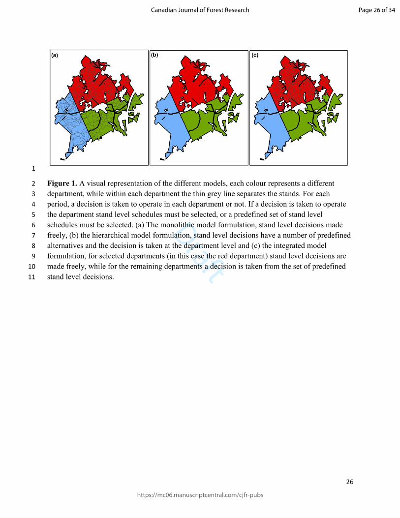
A graphical representation of the different optimization models and the types of decisions taken 1

for each model is provided in Figure 1. The problem represented in the figure consists of three 2

departments (separated by a thick black line), each with a variable number of stands (separated 3

by a thin grey line). In the first frame of the figure (a) represents the monolithic problem. In the 4

monolithic problem, a decision is made to determine during which period harvests will occur in 5

each department. Additionally, for each department, a decision is taken determining each stand 6

level schedule. The second frame (b) represents the top-level problem of the hierarchical model. 7

For each department, a set of department level solutions for each period is predefined (requiring 8

that harvesting stands can occur at that period), and the decision for this problem is to select the 9

department level solutions to optimize the objective function. The third frame (c) represents the 10

integrated hierarchical model, where features of both problems are integrated. For two of the 11

departments (green and blue), the decision is to select a department level solution. For the third 12

department (red) the stand level decisions must be made. At the department level, a decision is 13

to determine the timing of the harvest, and at the stand level to determine if a harvest should be 14

conducted. 15

16

Figure 1. 17

18

To add experimental context, we have created a synthetic version of this problem. This was 19

facilitated through use of a Jupyiter Notebook and the data consists of 1,000 artificial stands 20

simulated in the same manner as the real dataset. A wide range of variables can be adjusted, to 21

facilitate testing of the problem. The data and the Jupyiter Notebook can be found on the GitHub 22

repository at https://github.com/eyvindson/Hierarchical, details for the use of the tool is found at 23

Page 8 of 34



Draft

9

the repository. Using this tool, we evaluated a selection of cases, and provide results of this 1

evaluation in the supplementary material with the variables used identified in table S1, and the 2

results highlighted in figure S1. 3

4

For all models notation remains the same, and a list of the variables used can be found in Table 5

1. 6

7

Monolithic model: 8

The focus of the objective function is to obtain the required set of timber assortments at each 9

time period during the entire planning horizon. This was accomplished through a goal 10

programming approach, minimizing the weighted deviations from a set of targets set in the NRP 11

process. As goal programming problems may provide non-optimal solutions, we ensured 12

efficiency by including an augmentation term to select an optimal solution. For this case we 13

chose to focus on selecting the solution which minimizes all deviations from the targeted set of 14

timber assortments which has the highest net present income (NPI). In this case, the NPI is the 15

summation of the discounted income obtained from harvesting and silvicultural activities over 16

the planning horizon, and does not include potential discounted income past the planning 17

horizon. The potential for discounted income past the planning horizon is calculated as the 18

remaining productive value (PV), which if summed with NPI would equal the net present value 19

(the discounted income for an infinite planning horizon). The use of the small epsilon value is 20

used to ensure Pareto efficiency of the solution. While the primary objective is to minimize the 21

deviations away from the targeted timber assortments, if there are multiple solutions with similar 22

deviations the epsilon value promotes the solution with the highest NPI. Targets for yearly wood 23

Page 9 of 34



Draft

10

procurement were set at a species and assortment specific level. While the specific assortments 1

were important, a higher importance was set to the total yearly harvest level. Using the 2

predefined departments, a constraint was included to limit harvesting to once during the 10 year 3

planning horizon. These departments were originally created in order to divide the supervision 4

of harvests in Metsähallitus to local level managers. Here they were used to cluster harvests in 5

this study. 6

7

Objective function: 8

[1] min�� + ��∈� +�� + �� ∈��∈� − �� 9

Subject to: 10

[2] � � �� !

�"#�∈$%�∈& = (�� , forall0 ∈ 1, 2 ∈ 3

[3] (�� − �� + �� = 4�� , forall0 ∈ 1, 2 ∈ 3

[4] �(��∈� − �� + �� = 4��, forall2 ∈ 3

[5] �� !

�"5 ≤ 7�� , forall8 ∈ 9, : ∈ ;� , 2 ∈ 3

[6] �7��∈� ≤ 1, forall8 ∈ 9

[7] �� = � � ��=�� 1 + >��? �� !

�"#�∈��∈$%�∈&

Page 10 of 34



Draft

11

[8] �� !

�"# = 1, 8 ∈ 9, : ∈ ;�, 2 ∈ 3

[9] 7�� ∈ @0,1B, �� ∈ @0,1B, ��and�� ≤ 0DE>2 ∈ 3, �� and�� ≤ 0DE>0∈ 1, 2 ∈ 3

where �� and ��are the negative and positive deviations from the total periodic harvest target 1

(t), �� and �� are the negative and positive deviations from the periodic harvest target (t) for 2

each assortment (j), �� and �� are the weights associated with the total period harvest and the 3

periodic harvest for each assortment, � is a small positive number, �� is the net present income 4

obtained by implementing the plan, �� is the decision to select schedule k during time t for 5

stand s of department d, �� is the area of stand s in department d, �� is the per hectare 6

quantity of timber assortment j harvested from selecting schedule k during time t for stand s of 7

department d, (�� is the total quantity of timber assortment j harvested during period t from 8

implementing the chosen plan,4�� and 4�� are the targets for the total periodic harvest and the 9

periodic harvest target (t) for each assortment (j), 7�� is a variable indicating if harvests are 10

conducted in department d during time t, and =�� is the value in (€) of conducting schedule k 11

during time t for stand s in department d,>is the discount rate applied. The determination of the 12

weights can be elicited from the decision maker, and they can provide a prioritization between 13

the timing and timber assortments harvested. A variety of preference elicitation techniques are 14

available, for a sample of approaches used in forestry see Kangas et al. (2015). Equation [2] 15

calculates the harvests by period and timber assortments and period. Equation [3] is a goal 16

programming constraint, evaluating the negative and positive deviations from the targeted 17

harvest of each timber assortment. Equation [4] is a goal programming constraint, evaluating the 18

negative and positive deviations from the periodic flow of timber. Equation [5] is a constraint 19

Page 11 of 34



Draft

12

requiring that if any management schedule (other than the ‘do nothing’ option, when k= 1) then 1

harvests must be allowed during that period within the department. Equation [6] is a constraint 2

requiring that harvests occur only once in a department for the planning horizon. Equation [7] 3

calculates the NPI for the entire planning horizon for all stands under consideration. Equation 4

[8] is an area constraint, and equation [9] indicates the feasible region of the respective 5

variables. 6

7

From this monolithic model, the levels of the hierarchical plan can be formed. Special attention 8

must be made to ensure that appropriate constraints are placed in the correct hierarchical level. 9

10

Hierarchical models 11

We will first model the top-level problem in the hierarchy: 12

While the objective function of the top-level problem in the hierarchy is the same as the 13

monolithic problem [1], the details of how to calculate the required variables are different. 14

15

The top-level problem of the hierarchical model is subject to: 16

[10]

� � F�GG∈H%�∈& D��G� = (��forall0 ∈ 1, 2 ∈ 3

[11] � F�GG∈H%

= 1, forall8 ∈ 9

[12] �� = � � IF�G=�G� �1 + >��J KG∈H%�∈&

Page 12 of 34



Draft

13

[13] F�G ∈ @0,1B

and eqs 3,4,9. 1

Where F�G is the decision to conduct management actions for department d according to solution 2

z, D��G� is the quantity of timber assortment j at time period t for selecting solution z for 3

department d, =�G� is the value in (€) of selecting solution z during time t for department d. All 4

data used in this model is provide by the bottom level model, where the set of department level 5

solutions (L�) is populated by the solutions of bottom level models. Equations [10] and [12] 6

simply calculate the impact of selecting the specific department level solution on the quantity of 7

timber harvested and the NPI. Equation [11] requires that only one solution is selected for each 8

department. For this level, the calculations are very similar to the monolithic problem, and many 9

of the same equations can be integrated into the problem formulation. 10

11

The key element which is missing from the top-level problem is the set of department level 12

solutions which act as a dataset to the problem. While the monolithic problem utilizes stand 13

level simulations as the input data for the optimizations, the top-level problem requires 14

department level solutions as input data for the optimizations. Thus, an algorithm which 15

generates a predefined number of department level solutions is required. In Kangas et al. (2014) 16

the department level solutions were generated based on maximizing a linear weighted 17

combination of the NPI and the productive value after the planning horizon of the department. 18

This is justifiable as a wide range of alternative solutions will be produced with this scheme. 19

One issue with the use of weighting schemes to generate distinct solutions is that a 20

differentiation of weights does not guarantee unique solutions. 21

Page 13 of 34



Draft

14

1

To populate the department level solution dataset which is utilized in the optimization of the top-2

level hierarchical problem, we propose a solution generating scheme. The focus of this scheme 3

should be to produce a wide variety of unique department level solutions, to provide the 4

optimization tool a range of options to select. The scheme uses a model which is designed to 5

find solutions which span the range of the NPI, by maximizing the NPI while constrained to 6

ensure a specific productive value (PV; the remaining potential value of the forest after the 7

planning horizon, Pukkala 2015) which ranges between the theoretical minimum and maximum 8

PV. 9

10

Department level models (The bottom level, with separate models for each 8 ∈ 9 and each 11

2 ∈ 3): 12

Objective function: 13

[14] max��

Subject to: 14

[15] �N�� = � ��O�� 1 + >�#�? �� !

�"#�∈��∈$%

[16] �N�� ≥ �N�RSTUV + WX�N�UTYSZ,� − �N�RSTUV,�[

[17 ] �� = � ��=�� 1 + >��? �� !

�"#�∈$%

and equations 5, 6, 8 and 9. 15

where �N�� is the productive value of department d when the management actions are restricted 16

to time t, �N�UTYSZ,� and �N�RSTUV,� are the ideal and nadir values for the productive value of 17

Page 14 of 34



Draft

15

department d when the management actions are restricted to time t, O��is the productive value 1

of stand s of department d for schedule k and W is a parameter used to constrain the �N�� within 2

the feasible decision space, and where the symbol ‘#’ refers to the cardinality of the set. For this 3

model, the decision variables are to select the most appropriate harvest schedule at the stand 4

level decisions. Equations [5] and [6] ensure that all harvests in the department occur at a single 5

time period, while equation [8] is an area constraint and equation [9] provides the feasible range 6

for the parameters and variables. Each iteration provide a solution which contributes to the set of 7

department level solutions for the upper level problem (L�). 8

9

With this model, a wide range of department level solutions are possible. By focusing on the 10

importance of the NPI and PV, the aim is to focus on solutions which are economically 11

justifiable. Additionally, the timing of the harvests is restricted to a single period (t). However, it 12

is important to note that this scheme of developing solutions is rather myopic, and may not be 13

able to produce a full range of solutions required to ensure a high-quality top-level solution. 14

Creating a very wide range of department level solutions may provide an answer to ensure a 15

high-quality top-level solution, however this may be computationally burdensome as multiple 16

solution generating schemes each generating hundreds of solutions may be required. An 17

alternative method could be to generate department level solutions which fit within the specific 18

needs of the top level of the hierarchy. 19

20

Integrated hierarchical model: 21

As with the top-level problem, the objective function is the same as the monolithic model [1], 22

however the constraints require some adjustments: 23

Page 15 of 34



Draft

16

1

Subject to: 2

[18] � �F�GH%G"#�∈�&\]� D��G� + � � �� !

�"#�∈$^_∈] = (��, forall0 ∈ 1, 2 ∈ 3

[19]

�� = � �IF�G=�G� �1 + >��J KH%G"#�∈�&\]�+ � � ��`�_��_=_�� 1 + >��? a� !

�"#�∈��∈$^_∈]

3

and eqs 3, 4, 5, 6, 8, 9, 11 and 13, where b is a subset of the departments. For this model, there 4

are department level decision variables (F�G) which selects the most appropriate department 5

level solution and stand level decisions (��) which selects the most appropriate schedule for 6

those departments which has the complete data available within the model. Equation [18] 7

calculates the harvests by period and timber assortments and period, and equation [19] calculates 8

the NPI for the entire planning horizon for all stands under consideration. 9

10

This model combines both levels of the hierarchy together. As a starting point, the department 11

level solutions from the top-level problem are used, and the iterative approach incorporates a 12

selection of full department data into the top-level problem, creating a larger problem. For each 13

iteration the complete data for #bdepartment(s) are incorporated with top-level problem where 14

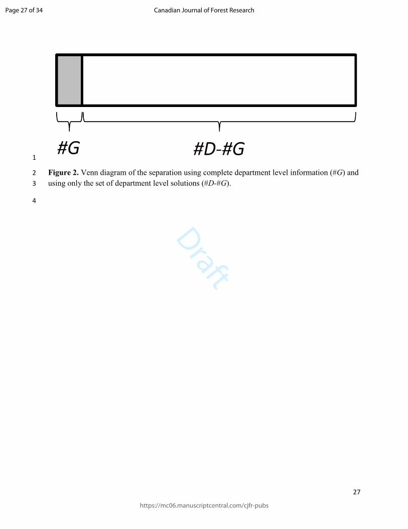
the #b department(s) are excluded. Using a Venn diagram (Figure 2), the separation of the 15

departments can be seen, with the grey section representing those departments with complete 16

information, and the white section being represented by the set of department level solutions. 17

Once a solution is found for this model, the solutions for each of the #bdepartment(s) are added 18

Page 16 of 34



Draft

17

as options for the department level solutions. With the added information, the gap between the 1

monolithic problem and this integrated hierarchical problem should decrease. 2

3

Results 4

All optimizations were made using a computer running a 64 bit version of Window 7, using an 5

Intel® Core ™ i7-4910MQ CPU at 2.9 GHz with 32 MB of RAM, running the optimization 6

software CPLEX version 12.6.2. 7

The monolithic plan: 8

Through the use of all stand level information at the regional level, the determination of when to 9

enter each department and the specific selection of how to manage each stand can be made. This 10

problem was optimized using CPLEX version 12.6.2. As a fairly complicated integer problem, 11

the expectation of finding the global solution was not anticipated, and we limited the 12

computation time to provide the best solution after 30 minutes. This choice was made following 13

experimental tests with longer time limits. While this stopping criterion may seem arbitrary, the 14

solution produced from the monolithic problem can be evaluated to be rather near the optimal 15

solution. As a goal programming problem, the focus of this model is to minimize the objective 16

function towards zero, and the objective values produced were rather near zero. When 17

calculating gap, CPLEX evaluates the gap as the absolute value of the (best node- best integer) 18

divided by the absolute value of best integer plus 1e-10. For goal programming calculations, 19

when the best integer is near zero the gap may not be reflective of the solutions ‘quality’. Each 20

of the periodic harvest targets were met with a maximum deviation of 0.94 m3 and harvest 21

assortment targets were met with a maximum deviation of 340 m3, and the NPI was 13,045,297 22

Page 17 of 34



Draft

18

€/year (Table 2). These results are compared to the performance of the hierarchical plans. As the 1

computation time was limited, this solution may not be the global optimal. 2

3

The bottom-up hierarchical plan without iterations: 4

This model requires the development of department level solutions. For each department a total 5

of 36 solutions were created. The parameter W was set to range from 0 to 1 with 0.2 intervals 6

between values and 6 solutions were found for each of the six time periods. Each department 7

level solution was solved to optimality within seconds. While solving the individual department 8

level problems was quick, a total of 5,184 problems needed to be solved to create the set of 9

solutions to be used in the top-level problem. Running several problems in parallel on the same 10

computer, we were able to solve all 5,184 problems in 9.5 minutes. 11

Once the solutions were created, the top-level problem could be solved. The hierarchical plan 12

was given 6 minutes to find a solution. As the hierarchical plan is an approximation, the 13

deviations from the target are substantially larger than for the monolithic plan. The periodic 14

harvests were achieved nicely with a maximum deviation of only 2 m3 (Table 2). The deviations 15

for the harvested assortments were substantially higher than for the monolithic plan, with a 16

maximum deviation for a single assortment at a single period of 23,211 m3. Due to the increased 17

deviations from the specific targets, the NPI had a higher value than the monolithic plan at 18

13,197,504 €/year. 19

The integrated hierarchical model: 20

This model is a continuation from the previous model. The modification is that the complete data 21

from a selection of departments is incorporated into the model. By including both hierarchies 22

Page 18 of 34



Draft

19

(even only a small subset of the bottom hierarchy) interactions between departments can be 1

captured, and improvements to the overall solution can be found. An iterative approach is used, 2

to allow for a variety of departments to be fully included into the integrated hierarchy. Following 3

the iteration, the department level solutions are included as data to the top level of the hierarchy. 4

To promote the iterative process, a time limit of 60 seconds for finding a solution was included 5

to the problem. This limit can be justified as the improvement from the inclusion of the full data 6

of other departments may improve the solution more quickly, than spending the time on 7

improving the specific department level solutions of the current iteration. 8

The iterative process can be visualized as a flowchart (Figure 3). To fully utilize the 9

computational power of the computer, multiple instances of the optimization were performed in 10

parallel. Each instance included a random selection of department level full data. This has the 11

added benefit of perhaps avoiding local level optimizations (Kirkpatrick et al. 1983). A total of 12

11 iterations were used as a stopping criterion, with the first point at iteration 0 indicating the 13

result when only the predefined department level solutions are used, i.e. the traditional hierarchic 14

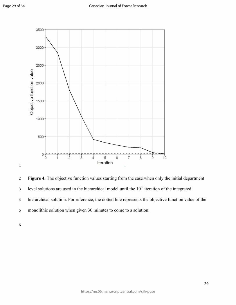
approach is used. The performances of the iterations are included in figure 4. After a single 15

iteration, the solution improves by 14%, and continues to improve dramatically for the next 4 16

cycles (an 87% improvement from the initial hierarchical solution), and then steady out rather 17

quickly. The best hierarchical solution has a very comparable solution to the monolithic problem. 18

For the iterative hierarchical plan, the periodic total harvests and the harvest assortment target 19

had a maximum deviation of 281 m3 from the set target and the harvest assortment target had a 20

maximum deviation of 633 m3 and the NPI was 12,829,531 €/year. The objective function value 21

for the monolithic solution was 18.67 and the hierarchical solution was 18.56 indicating that the 22

Page 19 of 34



Draft

20

hierarchical solution is negligibly better than the monolithic solution when given a limit of 30 1

minutes to find a solution. 2

3

Discussion 4

One of the key aims for hierarchical planning methods is to allow for the tractability of very 5

large problems. When the monolithic problem is feasible and solvable in a reasonable time, exact 6

methods should be used to find a solution. For cases when hierarchical planning is appropriate, 7

the solutions generated are not guaranteed to be optimal (or even nearly optimal), and methods 8

should be applied which strive for a quality solution. To accomplish this, the method should be 9

evaluated regarding the quality of the solution produced. For this case, we were able to use the 10

solution generated from monolithic problem as a benchmark for the performance of the 11

hierarchical plan. For cases when the solution to the monolithic problem is not available (which 12

may be the primary reason for utilization of hierarchical methods), a smaller (solvable) 13

representative problem may highlight the performance of the hierarchical approach. 14

The tested iterative approach markedly improved the performance of the traditionally used 15

hierarchic approach based solely on department-level solutions. Thus, when solving the problem 16

through a hierarchic formulation is the only possibility, it is recommendable to use the iterative 17

approach rather than the traditional bottom-up approach. The iterative approach could markedly 18

improve the usability of the hierarchic solution in practical applications. 19

The problem illustrated here is a simplification of the entire tactical planning process originally 20

formulated to provide solution acceptably close to the target values (Kangas et al. 2014). Some 21

of the constraints of the original strategic plan were not included, such as the targets for the 22

Page 20 of 34



Draft

21

volume of remaining broadleaved trees and the balancing of harvests between summer and 1

winter. Addition of constraints adds computational complexity to the problem. For instance, this 2

example did not consider the need to differentiate between conducting logging operations in 3

either summer or winter. As soil conditions may limit the ability to conduct logging operations, 4

this is often an important consideration when developing tactical level forest management plans. 5

Through a hierarchical planning approach, the inclusion of these types of constraints will make 6

the problem more difficult, however as long as the lower level problems can be solved; the entire 7

hierarchical problem will be solvable including the iterative hierarchical method. 8

The departments used in the study were quite large, meaning that the harvests clusters could be 9

too large to be acceptable (such as a large clear-cut area) or practical. On the other hand, the 10

harvests within a large department could be too widely scattered to serve as a proper clustering. 11

With the developed hierarchical approach, smaller departments defined based on the accessibility 12

of the stands from the main roads could be defined to further cluster the harvest. Moreover, the 13

test area included the area governed by Metsähallitus within one municipality (Kuhmo). Each 14

department represents the planning area for a single team, while the entire region is managed by 15

several teams. 16

In this case, we severely restricted the amount of time allocated to solving all of the more 17

computationally demanding optimization problems. For the monolithic and hierarchical 18

planning, this was done as the solution quality would only improve slightly if given more time. 19

For the iterative hierarchical planning, the allocation of time limits was done due to the trade-offs 20

between spending more time finding an optimal solution and improving the possible solution by 21

including different departments into the higher level optimization. As the iteration took 22

approximately 2 minutes to complete, with 10 iterations the iterative process took 20 minutes. If 23

Page 21 of 34



Draft

22

we add the time taken to generate the initial department level solutions, the iterative process took 1

a total of 30 minutes. In the studied case, the solutions generated with the monolithic and the 2

iterative hierarchical formulations are very similar using similar computational resources. 3

To evaluate the performance of the hierarchical process a tractable monolithic problem was used. 4

The results highlighted that for similar computational resources, the solution found by the 5

hierarchical process matched the solution found by the monolithic process in the studied case. 6

These solvable cases can be useful cases to provide guidance of how well the hierarchical 7

process works with similar but more difficult cases, extrapolation of how well the method 8

functions in solvable cases is valuable information. Thus, for applications to intractable 9

monolithic problems, the hierarchical method would still find a nearly optimal solution, if the 10

underlying sub-problems are solvable. 11

One such case could be the shift from a deterministic problem to a stochastic program, where the 12

tractability is generally a big issue (e.g. King & Wallace 2012). Solving a stochastic program 13

could be accomplished through a similar problem described in this paper. As the key difference 14

in stochastic problems is to incorporate uncertainty, how the uncertainty is tracked from the 15

stand levels to the department levels would be critical. The uncertainties at both levels in the 16

hierarchy need to be compatible, and must have some relationship to the objective function, or to 17

specific constraints which manage the specific risk aspect. For an exploration of hierarchical 18

stochastic methods readers are referred to the work of Pantuso, Fagerholt and Wallace (2015) 19

where they apply a hierarchical stochastic program to solving a fleet renewal problem. 20

Even in cases where the monolithic problem is tractable, there may be value in using a 21

hierarchical approach. For instance, interactive planning may require the development of updated 22

Page 22 of 34



Draft

23

solutions with a relatively quick solution time. Large tractable monolithic solutions may take 1

multiple hours or days to generate a single solution (Hartikainen et al. 2016). With the 2

hierarchical method, the initial steps of the iterative process (creating the predefined department 3

level solutions) can be done prior to integrating the decision makers into the process, and the 4

optimization problem can be adjusted, and re-solved using a few iterations. 5

Conclusions 6

Solving forest management problems through a hierarchical approach can find solutions which 7

are very close to the optimal solution for the monolithic problem. In this work, we formulate and 8

solve a monolithic regional forest planning problem which was intractable three years ago. We 9

then formulate and solve a bottom up hierarchical approach to the problem, and then develop and 10

solve an integrated hierarchical approach to the problem. The results highlight that when 11

problem complexity causes difficulties in finding a feasible solution, hierarchical planning may 12

be a useful tool to simplify the problem. Thus the hierarchical approach has potential for 13

increasing the use of spatial considerations in the practise and for allowing the use of landscape 14

level stochastic programming. 15

References 16

Bitran GR, Hax AC 1977. On the design of hierarchical production planning systems. Decision 17

Sciences, 8(1), 28-55. 18

Borges P, Kangas A., and Bergseng, E. 2017. Optimal harvest cluster size with increasing 19

opening costs for harvest sites. Forest Policy & Economics 75: 49–57. 20

Hartikainen M, Eyvindson K, Miettinen K, Kangas, A. 2016. Data-Based Forest Management 21

with Uncertainties and Multiple Objectives. In Pardalos P, Conca P, Giuffrida G, Nicosia 22

G. (Eds.), Machine Learning, Optimization, and Big Data : Second International 23

Page 23 of 34



Draft

24

Workshop, MOD 2016, Volterra, Italy, August 26-29, 2016, Revised Selected Papers (pp. 1

16-29). Lecture Notes in Computer Science, 10122. Springer. doi:10.1007/978-3-319-2

51469-7_2 3

Hiltunen, V., Kangas, J., Pykäläinen, J., 2008. Voting methods in strategic forest planning -4

experiences from Metsähallitus. Forest Policy and Economics 10: 117–127. 5

Hiltunen V, Kurttila M, Pykäläinen J. 2012. Strengthening top level guidance in geographically 6

hierarchical large scale forest planning: experiences from the Finnish state forests. Silva 7

Fenn. 46:539–554. 8

Hof JG, Pickens B. 1987. A pragmatic multilevel approach to large scale renewable resource 9

optimization: a test case. Nat Resour Model. 1:245–264. 10

Kangas A, Kurttila M, Hujala T, Eyvindson K, Kangas, J. 2015. Decision Support for Forest 11

Management. Second Edition. Springer. 12

Kangas A, Nurmi M, Rasinmäki J. 2014. From a strategic to a tactical forest management plan 13

using a hierarchic optimization approach. Scand J For Res. 29:sup1,154-165. 14

Kangas J, Store R, Leskinen P, Mehtätalo L. 2000. Improving the quality of landscape ecological 15

forest planning by utilizing advanced decision-support tools. For Ecol Manage, 132:157-16

171. 17

King, A.J. and Wallace, S.W. 2012. Modeling with stochastic programming. Springer, New 18

York. 19

Kirkpatrick S, Gelatt CD, Vecchie MP. 1983. Optimization by Simulated Annealing. Science 20

220:671-680. 21

Öhman K, Eriksson L-O. 2010. Aggregating harvest activities in long term forest planning by 22

minimizing harvest area perimeters. Silva Fenn. 44:77–89. 23

Page 24 of 34



Draft

25

Pantuso G, Fagerholt K, Wallace SW. 2014. Solving hierarchical stochastic programs: 1

application to the maritime fleet renewal problem. INFORMS Journal on Computing. 2

27(1):89-102. 3

Paradis G, LeBel L, D'Amours S, Bouchard M. 2013. On the risk of systematic drift under 4

incoherent hierarchical forest management planning. Can J For Res, 43(5): 480-492. 5

Pittman SB, Bare B, Briggs DG. 2007. Hierarchical production planning in forestry using price-6

directed decomposition. Can J For Res. 37:2010–2021. 7

Pukkala T (2005) Metsikön tuottoarvon ennustemallit kivennäismaan männiköille, kuusikoille ja 8

rauduskoivikoille (prediction models for productive value of pine, spruce and birch 9

stands in mineral soils). Metsätieteen aikakauskirja 3:311–322 [in Finnish] 10

Rasinmäki J, Kalliovirta J, Mäkinen A. 2009. SIMO: an adaptable simulation framework for 11

multiscale forest resource data. Comput Electron Agric 66:76–84 12

Smith S 1978. A two-phase method for timber supply analysis Proc. IUFRO Operational forest 13

management planning methods, Bucharest, Romania. 14

Virtanen H. 2010. Hakkuiden optimointi tiimitasolla Metsähallituksen metsissä [Master’s thesis]. 15

Department of Forest Resources Management, University of Helsinki. 59 p. + 16

appendices. 17

Weintraub A, Cholaky A. 1991. A hierarchical approach to forest planning. For Sci. 37:439–460. 18

Weintraub A, Guitart S, Kohn V 1986. Strategic planning in forest industries European J Oper 19

Res 24(1):152-162. 20

21

22

23

Page 25 of 34



Draft

26

1

Figure 1. A visual representation of the different models, each colour represents a different 2

department, while within each department the thin grey line separates the stands. For each 3

period, a decision is taken to operate in each department or not. If a decision is taken to operate 4

the department stand level schedules must be selected, or a predefined set of stand level 5

schedules must be selected. (a) The monolithic model formulation, stand level decisions made 6

freely, (b) the hierarchical model formulation, stand level decisions have a number of predefined 7

alternatives and the decision is taken at the department level and (c) the integrated model 8

formulation, for selected departments (in this case the red department) stand level decisions are 9

made freely, while for the remaining departments a decision is taken from the set of predefined 10

stand level decisions. 11

Page 26 of 34



Draft

27

1

Figure 2. Venn diagram of the separation using complete department level information (#G) and 2

using only the set of department level solutions (#D-#G). 3

4

Page 27 of 34



Draft

28

1

2

Figure 3. The flow of information with the different models, and the interaction between models 3

and data to calculate a solution. At the start of the process, the only data present is the stand level 4

data. The department level data is filled as the bottom level models are solved. 5

Page 28 of 34



Draft

29

1

Figure 4. The objective function values starting from the case when only the initial department 2

level solutions are used in the hierarchical model until the 10th iteration of the integrated 3

hierarchical solution. For reference, the dotted line represents the objective function value of the 4

monolithic solution when given 30 minutes to come to a solution. 5

6

Page 29 of 34



Draft

30

Table 1. A list of notation used throughout the paper. 1

Symbol Definition

Sets 9 Set of departments selected b Set of the departments 1 Set of timber assortments under consideration c�� Set of schedules for stand s in time t ;_ Set of the stands in department g 3 Set of the time periods under consideration L� Set of solutions for department d Data �� The area of stand s in department d �� The amount of timber assortment j available for harvest by selecting schedule k

during time t for stand s of department d O�� Productive value of stand s of department d for schedule k =�� The value of conducting schedule k during time t in stand s of department d

Variables D��G� The quantity of timber assortment j at time t for solution z of department d (�� Total quantity of timber assortment j harvested during period t 7�� Binary variable indicating if harvests are conducted in department d during time t �� , �� Negative (positive) deviations from the total periodic harvest target (t) �� , �� Negative (positive) deviations from the periodic harvest target (t) for each assortment (j) �� Net present income for the plan �N�� Productive value for department d at time t (scripts indicate also ideal and nadir values) =�G� The value of selecting solution z during time t for department d

Decision variables �� The decision to manage the stand s in a specific department d according to schedule k during time t F�G The decision to conduct management actions in department d according to solution z

Parameters 4��, 4�� Targets for the total period harvest (α) and the periodic harvest for each assortment (β) � A very small number, used for the augmentation term > The discount rate �� , �� Weights associated with the total period harvest (α) and the periodic harvest for each assortment (β) W A parameter to constrain the solutions within the feasible decision space associated with the productive value of the department

2

Page 30 of 34



Draft

31

Table 2. The average annual results for the different problem formulations. 1

2

Page 31 of 34



Draft

Supplementary material to:

Evaluating a hierarchical approach to landscape level harvest scheduling by Kyle Eyvindson,

Juusi Rasinmäki and Annika Kangas

This supplementary document uses synthetic data to test to computational requirements and

performance of the different hierarchical models. The methods and data used in this analysis are held in

a GitHub repository at https://github.com/eyvindson/hierarchical

The entire process was modelled in Python, using the Pyomo package (Hart et al. 2012) to model the

problem and link the model to a commercial optimization package (CPLEX 12.6 in this case). A set of

1,000 artificial stands were generated to represent potential initial conditions, and these stands were

simulated for 10 years through 6 periods (four one-year periods and two three-year periods). This

dataset can be combined to represent a wide variety of forest sizes.

The Python code is partitioned in to six sections:

1. List of variables used throughout code:

All variables which influence the optimization process and the re-structuring of the data are

included here. A change in these variables will increase/decrease the computational complexity

of the problem, and increase/decrease the amount of time allocated to the different

optimizations.

2. Adding packages

Here all of the importing of python packages is done.

3. Create optimization functions

Each of the optimization functions are created with a separate function. Pyomo is used to

create the models, and each optimization model reflects the models created in the

manuscript.

4. Importing data

The set of 1000 synthetic stands are imported through Pandas. Users need to ensure that the

path and data file name reflects their system.

5. Creating structured data for optimization

Here the synthetic stands are organized into a data frame which reflect the problem

structure. A number of departments are created with a random number of stands (bounded

between a minimum and maximum value). The area of each stand is also a random value,

bounded between a minimum and maximum value.

Page 32 of 34



Draft

6. Solving the optimization problems

Each of the models are sent to the optimization software (in this case CPLEX), and given a set

amount of time to process.

To provide context for the target values, the monolithic problem is solve to find the maximum

possible amount of timber produced during the entire period, and is resolved using a

percentage of that maximum as a target for each period. With a synthetic dataset, setting

appropriate targets can be difficult as the specific case changes with the random variables.

Once solved, the objective function is provided, and the time taken to generate the solutions is

also provided.

For this supplementary material three cases with increasing complexity were solved, we provide the

variables used in table S1 and solutions to each of the problems is found in Figure S1.

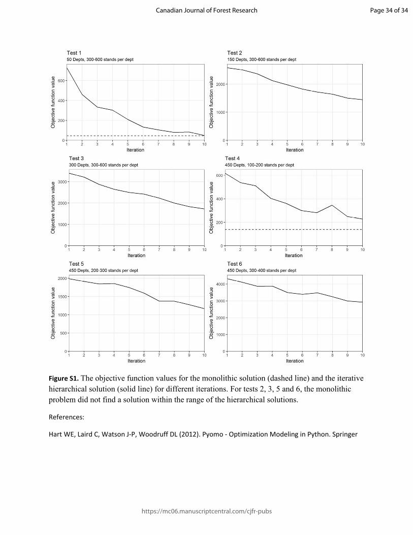
Table S1. Adjustment of a selection of variables used in the six different tests.

Variables adjusted

Depts min_stands max_stands

Test 1 50 300 500

Test 2 150 300 500

Test 3 300 300 500

Test 4 450 100 200

Test 5 450 200 300

Test 6 450 300 400

The results and performance of the different models are highlighted in Figure S1. The results are similar

to that found in the manuscript, with the large problems (when the departments in the analysis are 300)

showing that the monolithic problem does not come close to the global solution under the time limits

provided. This is seen as the integrated model finds better solutions than what has been produced

through the monolithic model.

Page 33 of 34



Draft

Figure S1. The objective function values for the monolithic solution (dashed line) and the iterative

hierarchical solution (solid line) for different iterations. For tests 2, 3, 5 and 6, the monolithic

problem did not find a solution within the range of the hierarchical solutions.

References:

Hart WE, Laird C, Watson J-P, Woodruff DL (2012). Pyomo - Optimization Modeling in Python. Springer

Page 34 of 34



Documents

system appendPDF cover-forpdf · 12 planning was suggested by Bitran and Hax (1977) as a means to solve a production scheduling 13 problem