Embed Size (px)
Citation preview

System Analysis, Modelling and Controlwith Polytopic Linear Models

CIP-DATA LIBRARY TECHNISCHE UNIVERSITEIT EINDHOVEN
Angelis, Georgo Z.
System Analysis, Modelling and Control with Polytopic Linear Models /by Georgo Z. Angelis. -Eindhoven : Technische Universiteit Eindhoven, 2001.Proefschrift. - ISBN 90-386-2672-XNUGI 851Trefwoorden: polytopic linear models / niet-lineaire systemen / lineaire sys-temen / regelsystemen; stabiliteit / regelsystemen; prestatie / regelsystemen;gain schedulingSubject headings: polytopic linear models / nonlinear systems / linear systems/ control systems; stability / control systems; performance / control systems;gain scheduling
Printed by the Universiteitsdrukkerij TU Eindhoven, The NetherlandsCover design by Ben Mobach
Copyright c© 2001 by G.Z. AngelisAll rights reserved. No parts of this publication may be reproduced or utilizedin any form or by any means, electronic or mechanical, including photocopy-ing, recording or by any information storage and retrieval system, withoutpermission of the copyright holder.

System Analysis, Modelling and Controlwith Polytopic Linear Models
PROEFSCHRIFT
ter verkrijging van de graad van doctoraan de Technische Universiteit Eindhoven,
op gezag van de Rector Magnificus,prof.dr. M. Rem, voor een commissie
aangewezen door het College voor Promotiesin het openbaar te verdedigen op
dinsdag 6 februari 2001 om 16.00 uur
door
Georgo Z. Angelis
geboren te Berghem

Dit proefschrift is goedgekeurd door de promotoren:
prof.dr.ir. J.J. Kokenprof.dr. H. Nijmeijer
Copromotor:dr.ir. M.J.G. van de Molengraft

Contents
Summary ix
Acknowledgments xi
1 Introduction 11.1 Motivation . . . . . . . . . . . . . . . . . . . . . . . . . . . . . 11.2 Overview of the Study . . . . . . . . . . . . . . . . . . . . . . . 5
I ANALYSIS 7
2 Introduction to Analysis 9
3 Model and Interpretations 113.1 Introduction . . . . . . . . . . . . . . . . . . . . . . . . . . . . . 113.2 Polytopic Model Structure . . . . . . . . . . . . . . . . . . . . . 113.3 Optimal Model Structure . . . . . . . . . . . . . . . . . . . . . 153.4 Interpretations . . . . . . . . . . . . . . . . . . . . . . . . . . . 163.5 Model Based Interpretations . . . . . . . . . . . . . . . . . . . . 173.6 Knowledge Based Interpretation . . . . . . . . . . . . . . . . . 213.7 Notes and Comments . . . . . . . . . . . . . . . . . . . . . . . . 24
4 Approximation 274.1 Introduction . . . . . . . . . . . . . . . . . . . . . . . . . . . . . 274.2 A Universal Approximator . . . . . . . . . . . . . . . . . . . . . 294.3 Upper bound on the Number of Models . . . . . . . . . . . . . 324.4 Upper bound on the Difference between Trajectories . . . . . . 344.5 Systems with Inputs . . . . . . . . . . . . . . . . . . . . . . . . 354.6 Systems with Structure . . . . . . . . . . . . . . . . . . . . . . 404.7 Notes and Comments . . . . . . . . . . . . . . . . . . . . . . . . 52
v

vi Contents
5 Stability, Controllability and Observability by Duality 555.1 Introduction . . . . . . . . . . . . . . . . . . . . . . . . . . . . . 555.2 Lyapunov Stability . . . . . . . . . . . . . . . . . . . . . . . . . 565.3 Stability of a PLM and Implications for the System . . . . . . . 605.4 Controllability . . . . . . . . . . . . . . . . . . . . . . . . . . . 655.5 Observability by Duality . . . . . . . . . . . . . . . . . . . . . . 715.6 Notes and Comments . . . . . . . . . . . . . . . . . . . . . . . . 74
II MODELLING 77
6 Introduction to Modelling 796.1 Model Building . . . . . . . . . . . . . . . . . . . . . . . . . . . 806.2 Experiment Design . . . . . . . . . . . . . . . . . . . . . . . . . 816.3 Model Construction . . . . . . . . . . . . . . . . . . . . . . . . 826.4 Model Validation . . . . . . . . . . . . . . . . . . . . . . . . . . 85
7 Building PLMs from known Nonlinear Models 897.1 Introduction . . . . . . . . . . . . . . . . . . . . . . . . . . . . . 897.2 From Operating Space to Scheduling Space . . . . . . . . . . . 917.3 From Scheduling Space to Scheduling Regimes . . . . . . . . . 927.4 From Scheduling Regimes to PLM Parameters . . . . . . . . . 957.5 Examples . . . . . . . . . . . . . . . . . . . . . . . . . . . . . . 987.6 Notes and Comments . . . . . . . . . . . . . . . . . . . . . . . . 108
8 Building PLMs from Measured Data 1118.1 Introduction . . . . . . . . . . . . . . . . . . . . . . . . . . . . . 1118.2 Least Squares Filtering . . . . . . . . . . . . . . . . . . . . . . . 1128.3 Local Parameter Estimation . . . . . . . . . . . . . . . . . . . . 1148.4 Example . . . . . . . . . . . . . . . . . . . . . . . . . . . . . . . 1178.5 Global Parameter Estimation . . . . . . . . . . . . . . . . . . . 1218.6 Example . . . . . . . . . . . . . . . . . . . . . . . . . . . . . . . 1238.7 Notes and Comments . . . . . . . . . . . . . . . . . . . . . . . . 127
III CONTROL 129
9 Introduction to Control 131
10 Friction Compensation for a Rotational Robotic ManipulatorSystem 13310.1 Introduction . . . . . . . . . . . . . . . . . . . . . . . . . . . . . 13310.2 A PLM Representing a Rotational Robotic Manipulator System 134
Contents vii
10.3 Nonlinear State Feedback Friction Compensation . . . . . . . . 13410.4 Experiments . . . . . . . . . . . . . . . . . . . . . . . . . . . . . 13510.5 Conclusion . . . . . . . . . . . . . . . . . . . . . . . . . . . . . 136
11 Optimal Control 13711.1 Introduction . . . . . . . . . . . . . . . . . . . . . . . . . . . . . 13711.2 Stabilizing Optimal Controls . . . . . . . . . . . . . . . . . . . 13811.3 Inverse Optimal Controls . . . . . . . . . . . . . . . . . . . . . 14111.4 Optimal Control of a Translational Inverted Pendulum on a Cart14211.5 Notes and Comments . . . . . . . . . . . . . . . . . . . . . . . . 144
12 Adaptive Optimal Friction Control for a Robotic ManipulatorSystem 14912.1 Introduction . . . . . . . . . . . . . . . . . . . . . . . . . . . . . 14912.2 A PLM Representing a Rotational Robotic Manipulator System 15012.3 Adaptive Optimal Control . . . . . . . . . . . . . . . . . . . . . 15212.4 Experiments . . . . . . . . . . . . . . . . . . . . . . . . . . . . . 15612.5 Conclusion . . . . . . . . . . . . . . . . . . . . . . . . . . . . . 158
13 Robust Control with Bounds on Performance 15913.1 Introduction . . . . . . . . . . . . . . . . . . . . . . . . . . . . . 15913.2 State-space Partitioning and Feedback Law . . . . . . . . . . . 16013.3 Performance and Bounds on the Associated Cost . . . . . . . . 16213.4 Controller Synthesis . . . . . . . . . . . . . . . . . . . . . . . . 16613.5 Example . . . . . . . . . . . . . . . . . . . . . . . . . . . . . . . 16813.6 Conclusion . . . . . . . . . . . . . . . . . . . . . . . . . . . . . 171
14 Conclusions 17314.1 Main Conclusions . . . . . . . . . . . . . . . . . . . . . . . . . . 17314.2 Main Contributions . . . . . . . . . . . . . . . . . . . . . . . . . 17414.3 Suggestions for further Research . . . . . . . . . . . . . . . . . 175
Bibliography 177
List of Acronyms 185
Some Symbols 187
Index 189
Samenvatting 191

viii Contents

Summary
This research investigates the suitability of Polytopic Linear Models (PLMs)for the analysis, modelling and control of a class of nonlinear dynamical sys-tems. The PLM structure is introduced as an approximate and alternativedescription of nonlinear dynamical systems for the benefit of system analysisand controller design. The model structure possesses three properties that wewould like to exploit.
Firstly, a PLM is build upon a number of linear models, each one of whichdescribes the system locally within a so-called operating regime. If thesemodels are combined in an appropriate way, that is by taking operating pointdependent convex combinations of parameter values that belong to the dif-ferent linear models, then a PLM will result. Consequently, the parametervalues of a PLM vary within a polytope, and the vertices of this polytope arethe parameter values that belong to the different linear models. A PLM owesits name to this feature. Accordingly, a PLM can be interpreted on the basisof a regime decomposition. Secondly, since a PLM is based on several linearmodels, it is possible to describe the nonlinear system more globally comparedto only a single linear model. Thirdly, it is demonstrated that, under the ap-propriate conditions, nonlinear systems can be approximated arbitrary closeby a PLM, parametrized with a finite number of parameters. There will begiven an upper bound for the number of required parameters, that is sufficientto achieve the prescribed desired accuracy of the approximation.
An important motivation for considering PLMs rests on its structural sim-ilarities with linear models. Linear systems are well understood, and theaccompanying system and control theory is well developed. Whether or notthe control related system properties such as stability, controllability etcetera,are fulfilled, can be demonstrated by means of (often relatively simple) math-ematical manipulations on the linear system’s parameterization. Controllerdesign can often be automated and founded on the parameterization and thecontrol objective. Think of control laws based on stability, optimality and soon. For nonlinear systems this is only partly the case, and therefore furtherdevelopment of system and control theory is of major importance. In viewof the similarities between a linear model and a PLM, the expectation exists
ix

x Summary
that one can benefit from (results and concepts of) the well developed linearsystem and control theory. This hypothesis is partly confirmed by the resultsof this study.
Under the appropriate conditions, and through a simple analysis of theparametrization of a PLM, it is possible to establish from a control perspectiverelevant system properties. One of these properties is stability. Under theappropriate conditions stability of the PLM implies stability of the system.Moreover, a few easy to check conditions are derived concerning the notionof controllability and observability. It has to be noticed however, that theseconditions apply to a class of PLMs of which the structure is further restricted.
The determination of system properties from a PLM is done with theintention to derive a suitable model, and in particular to design a model basedcontroller. This study describes several constructive methods that aim atbuilding a PLM representation of the real system.
On the basis of a PLM several control laws are formulated. The mainobjective of these control laws is to stabilize the system in a desired operatingpoint. A few computerized stabilizing control designs, that additionally aimat optimality or robustness, are the outcome of this research.
The entire route of representing a system with an approximate PLM, sub-sequently analyzing the PLM, and finally controlling the system by a PLMbased control design is illustrated by means of several examples. These exam-ples include experimental as well as simulation studies, and nonlinear dynamic(mechanical) systems are the subject of research.

Acknowledgments
I am very appreciative to a number of people that have been involved in therealization of this thesis. I would like to thank a number of them here, realizingthat such a list will never be exhaustive.
First of all, I would like to thank my promotor Jan Kok as one of theinitiators of the project for his faith and support during the entire researchproject. I am also grateful to my promotor Henk Nijmeijer for the manystimulating in-depth discussions we had. He also continuously provided mewith valuable comments. This book was greatly improved by the suggestionsof my copromotor Rene van de Molengraft. He has been a great source ofinspiration and with his enthusiasm he also encouraged me to write this book.
I thankfully acknowledge the support of the students Geert de Goeij, RonHensen, Peter Jacobs, Ramidin Kamidi, Patrick Stapel, Rick Tebbens, AlexThissen, Joris Verstraete and Casper Wassink who graduated on this projectand made valuable contributions to the subject.
Also, I want to thank my colleagues Annelies Balkema, Ron Hensen, RoelLipsch, Patrick Philips, Gerwald Verdijck and Mathieu Westerweele from theControl group of the faculties of Applied Physics and Mechanical Engineeringat Eindhoven University of Technology for the friendly atmosphere.
Especially, I would like to thank my parents for their love and support.They taught me ‖·‖ of life.
Last but not least, I thank my wife Marjon and my daughter Evvi, fortheir patience and understanding during the long time that this project took.
Georgo AngelisEindhoven, November 2000.
xi

xii Acknowledgments
Chapter 1
Introduction
This thesis describes a systematic and creative approach towards the analysis,modelling and control of a broad class of nonlinear systems. Polytopic linearmodels are introduced to represent the system under investigation, and thepotential that these models offer for system analysis, modelling and control isexplored in detail. In this introductory chapter we give a motivation for thisthesis, outline the major themes to be explored and developed in subsequentchapters, and it describes how the study is organized.
1.1 Motivation
Mathematical models, abstractions of real life systems, are of great importancefor the understanding of system behavior. From a control engineering point ofview it is of great interest how to choose the system inputs, such that desiredcontrol objectives are met. The intended application of a model, in our casecontrol, will impose restrictions on its structure and complexity. There is atrade-off, since models that can be analyzed and dealt with within a controlscheme are often inaccurate, and models that reflect system behavior moreaccurately are often too complex to analyze and deal with within a controlscheme.
Model paradigms
Models that relate observed variables (inputs and outputs) by means of astate-space description are common in systems and control theory. Accordingto such a model, at each time instant, the state variables summarize all ofthe information needed in order to predict together with the future inputs,the future evolution of the system in time. The dynamics of a large classof nonlinear dynamical systems may be cast by a set of nonlinear first order
1

2 Introduction
differential equations together with a nonlinear algebraic output equation asfollows:
x = f(x, u) (1.1)y = h(x, u)
with the state x ∈ X ⊆ Rn, the manipulated input u ∈ U ⊆ R
m, and theoutput y ∈ Y ⊆ R
p.It is clear that systems as described by (1.1) are more general than their
linear time invariant (LTI) counterparts:
x = Ax + Bu (1.2)y = Cx + Du
However a large part of the control literature is devoted to linear systems andmany linear system theoretic properties and control problems have been sat-isfactory dealt with in the literature [67], [41]. There are two main reasonsfor studying linear systems for the purpose of control. Firstly, linear systemsare parametrized, and system properties can be revealed easily by analysis ofits representation (A, B, C, D). Furthermore, for linear systems the availableanalysis tools enable strong results on system and control theoretic propertiessuch as stability, controllability, observability, optimality, robustness etc.. Sec-ondly, first order approximations are in many cases sufficient to characterizethe local behavior of the nonlinear system. This means that often analysisbased on linearizations reveals properties of the system locally, and designsbased on linearizations often work locally for the original system [67]. This‘linearization principle’1 restricts the applicability of the linear model sincedesirable and expected behavior of the system can only be guaranteed foroperating conditions that are close to the point of linearization. This fact,together with the problem of characterizing system properties, for which theanalysis based on its linearization fails, motivated researchers to study non-linear models, with the intention to derive stronger results, confer [57], [65].Much research effort is directed towards that goal, and since it is not just amatter of extending the linear theory, new concepts are needed.
Instead of studying the general nonlinear model (1.1) to enlarge the appli-cability compared to the linear model we will follow another approach basedon the linearization principle mentioned above. The idea behind the approachis simple and several researchers and application oriented engineers have comeup with similar ideas, confer [55], [34], [71].
1The linearization principle is made precise in [67]. Sufficient conditions for local stability,controllability and observability of the system (1.1) are derived based on the parametrization(A, B, C, D) of the linearization (1.2) of the system (1.1).

1.1 Motivation 3
The basic idea is to linearize (1.1) at several specific operating conditions.The operating conditions are chosen in such a way that the correspondinglinear models reflect the qualitatively different behavior in these operatingregimes. The operating regimes cover the full operating space. To mimic thebehavior of the general nonlinear model, the different linear models obtainedfor different operating conditions are scheduled in the operating-space, as be-havior changes qualitatively under varying operating conditions. Schedulingin this case means forming convex combinations of locally valid linear models.In this way a more global model is obtained that approximately reflects the be-havior of the general model for the full range of operation. The resulting modelis represented by a finite number Nm of linear models (Ai, Bi, ai, Ci, Di, ci)together with corresponding scheduling functions wi(x, u) as follows
x =Nm∑i=1
wi(x, u)Aix + Biu + ai
y =Nm∑i=1
wi(x, u)Cix + Diu + ci(PLM)
with
Nm∑i=1
ωi(x, u) = 1 and ωi(x, u) ≥ 0 for all (x, u) ∈ X × U
These nonlinear models frequently occur in literature and although of anequivalent mathematical structure they are given different names such as FuzzyModels [69], [86], Multi-Models [55] or Local Model Networks [38]. The modelstructure has several desirable attributes that we would like to exploit. Firstof all, the model class is rich since a large class of nonlinear systems can beapproximated arbitrarily close with the proposed model structure [86], [38].Secondly, the model is interpretable on the basis of a regime decomposition[69], [38]. Also the model has an a priori fixed structure, that shows similaritieswith linear systems. The obtained model is called a Polytopic Linear Model(PLM) since the model consists of a set of representations of linear models thatdefine a polytope in the models parameter-space, which will become clear lateron.
Trade-off
Especially within the area of systems and control engineering, the diversity ofthe intended model applications, such as system analysis, controller synthesisand simulation puts high demands on the model. As mentioned earlier, repre-senting a system with an accurate mathematical description of its dynamical

4 Introduction
properties that is also simple to use for the intended application at hand, re-sults in conflicting demands. On one hand, general nonlinear models can bevery accurate but as a result of their complexity difficult to build from firstprinciples and data. Furthermore, these models are difficult to analyze andto apply in model based control schemes. So, these models are not simple.On the other hand LTI systems are well understood, but are at most locallyvalid in representing an actual system, i.e. incorrect conclusions may be drawnfrom it, resulting in an unsuccessful control strategy. In the ideal situation,one would like to build a model that is as accurate as the most detailed math-ematical model and as simple as a LTI system in the sense as described before.This situation is sketched in Figure 1.1.
accu
racy
complexity
general nonlinearmodel
ideal modelfor control
LTI model
low
low
high
high
PLMs
Figure 1.1: The PLM is an alternative compromise between the conflictingdemands, accuracy and complexity. Every candidate model is within the greyregion. The best candidate model is the one closest to the ideal model.
The ideal model as indicated in this figure does of course not exist. Thechoice for a general nonlinear model or a LTI model to represent the systemfor the intended application in mind are just two possibilities out of numerouspossible compromises between complexity and accuracy. The PLM is an al-ternative compromise between these two conflicting demands that lies withinthe shaded region in Figure 1.1. The intended application of the model, in ourcase control, imposes demands on the model to be selected. The choice for afixed and flexible model structure that locally shows similarities with LTI sys-tems, hopefully enlarges the possibility to develop systems and control theory,and model building methodologies. This hypothesis motivates to explore thesuitability of the PLM as a candidate model structure for model based controlapplication. Suitability involves interpretability, representation capacity, andthe analysis and controller synthesis abilities as explored in this thesis. Asa consequence, it is to be expected that as a result of further research, the

1.2 Overview of the Study 5
distance between the ideal model and the PLM will decrease further in thefuture. This will probably increase the number of applications for which thePLM is the minimizer of the distance between the ideal model and a memberof the set of all candidate model structures.
1.2 Overview of the Study
This thesis describes a systematic approach for the analysis, modelling andcontrol of a broad class of nonlinear systems, and consists of three main parts.
The first part, Part I, explores the system analysis potential of PLMsthat are relevant for model based control application. In Chapter 3, the PLMstructure will be introduced and its interpretations are explained. In Chapter 4the approximation properties of PLMs are investigated. After that, in Chapter5, properties will be explored that are relevant for system analysis and controlpurpose, such as stability, controllability and observability of a PLM.
The second part, Part II, investigates the modelling power of PLMs anddescribes in detail, how to construct a systems model with the desired PLMstructure. In Chapter 7, a model based modelling method is considered. Itis assumed that a nonlinear model of the system is available. In Chapter8, two data based modelling methods are considered. It is assumed thatmeasurements have been obtained from the system.
The last part, Part III, examines the model based control capabilities ofPLMs. The acquired knowledge from the previous parts, will be utilized infour experimental and simulation case-studies, to design controllers for non-linear systems that meet pre-imposed control objectives. In Chapter 10, afriction compensator design for a real rotational robotic manipulator systemis reported. In Chapter 11, an optimal regulator design is reported. In Chap-ter 12, a model based controller design will be proposed with the objective toperform servo tasks on mechanical systems that exhibit friction. Again thecontrol of a real rotational robotic manipulator system is considered. In Chap-ter 13, a stabilizing controller is designed for a family of (nonlinear) systems.The controller is robust against parametric uncertainty of the system.
The final chapter, Chapter 14, contains the main conclusions, summarizesthe main contributions, and gives some suggestions for further research.

6 Introduction

Part I
ANALYSIS
7

Chapter 2
Introduction to Analysis
In this part the analysis of PLMs, that are relevant for model based controlapplications, are explored in detail.
In Chapter 3, the PLM structure is introduced and its interpretations areexplained. In Chapter 4, the approximation properties of PLMs are inves-tigated. After that, in Chapter 5, properties are explored that are relevantfor system analysis and control purpose, such as stability, controllability andobservability of a PLM.
9

10 Introduction to Analysis

Chapter 3
Model and Interpretations
3.1 Introduction
In this chapter the PLM is introduced and its interpretations are explainedin detail. We will start building on the results obtained in [34], where theidea of patching together locally valid models was formalized, and was givena theoretical foundation.
In Section 3.2, the polytopic model structure will be introduced on thebasis of a regime decomposition of the operating space of a nonlinear system.After that, in Section 3.3, it is shown that the proposed PLM structure isoptimal in an appealing sense. In Section 3.4, the model based and knowledgebased interpretation of the PLM is introduced. In Section 3.5, a more in depthdescription of the several model based interpretations is given. In Section3.6, the knowledge based interpretation of the PLM is clarified. Finally, inSection 3.7, some notes and comments are made regarding the presented modelstructure and interpretation.
3.2 Polytopic Model Structure
Suppose we want to characterize the behavior of
x = f(x, u, v) (3.1)y = h(x, u, v)
with the state x ∈ X ⊆ Rn, the manipulated input u ∈ U ⊆ R
m, the observedauxiliary variable v ∈ V ⊆ R
l and the output y ∈ Y ⊆ Rp. Then within a suf-
ficient small region Xi×Ui×Vi around (xi, ui, vi), a first order approximation,a linear model Mi obtained by a Taylor linearization of (3.1) in (xi, ui, vi), that
11
12 Model and Interpretations
is
x = fi(x, u, v) (3.2)
= f(xi, ui, vi) +∂f
∂x(xi, ui, vi)(x− x0i) +
∂f
∂u(xi, ui, vi)(u− u0i)
+∂f
∂v(xi, ui, vi)(v − v0i)
y = hi(x, u, v)
= h(xi, ui, vi) +∂h
∂x(xi, ui, vi)(x− x0i) +
∂h
∂u(xi, ui, vi)(u− u0i)
+∂h
∂v(xi, ui, vi)(v − v0i)
will give an approximate description of the system, provided the system is atleast differentiable with respect to its arguments. At this stage the operatingspace Ψ = X × U × V with operating vector ψ ∈ Ψ is introduced, and it isassumed that Mi has a range of validity Ψi ⊂ Ψ.
A model (3.2) that has a range of validity1 less than the desired range ofvalidity will be called a local model, as opposed to a global model that is validin the full range of operation. If now the models are chosen in such a way thatΨ ⊆ (∪iΨi) then the models can be combined to form a globally valid model.
Often it is not necessary to characterize a validity region for a model withinthe (high dimensional) operating space. Therefore the scheduling space Z,consisting of the set of scheduling variables z ∈ Z is introduced. A schedulingvector z, consists of variables that schedule the models, that means influencesvalidity of Mi. In many cases there will exist a function s : Ψ = X×U×V → Zthat projects ψ onto a lower dimensional scheduling space Z, thus z = s(ψ)with dim(z) < dim(ψ). The region in which a model is valid is called anoperating regime, that is Ψi = ψ ∈ Ψ | s(ψ) ∈ Zi. The corresponding regionZi is called a scheduling regime.
The framework can be conceptually illustrated as in Figure 3.1. Beforeproceeding with the question on how to combine the models obtained for thedifferent regimes into a global model, let us first illustrate the above terms,such as operating space and scheduling regime, by means of an example.
Example 3.2.1 Consider the pendulum without friction in Figure 3.2.Its dynamics is described by
Jθ −mgl sin θ = τ (3.3)
1The term ‘valid ’ has not been clarified at this stage and of course depends upon thepurpose of modelling. In our case validity of the model will be related to a measure ofcloseness to the real system in such a way that they share the same qualitative structure orsome system properties, at least locally.

3.2 Polytopic Model Structure 13
z1
z2
Z1
Z2
Z3
Z4
Z
Figure 3.1: The system’s full range of operation, is completely covered bya number of possibly overlapping operating regimes Ψi. The models Mi arescheduled within the lower dimensional scheduling space Z ⊆ (∪i∈1,..,4Zi).In each operating regime the system is modelled by a linear state-space model.z ∈ Z is typically a subset of the variables that constitute ψ. One could thinkof the remaining variables of ψ being on any axis perpendicular to z therebynot influencing validity of a specific model.
where m is the mass of the ball, the mass of the stick is neglected, g is the grav-ity, l is the (variable) position of the ball, and θ is the angle of the pendulumwith the vertical axis. If we write (3.3) in the form of (3.1) we obtain
x1 = x2 (3.4)
x2 =mg
Jv sinx1 +
1J
u
with x1 = θ, x2 = θ, u = τ and v = l and x ∈ X, u ∈ U and v ∈ V . Firstassume that the position of the ball is fixed, i.e. l can be viewed as a constantparameter. Then the operating space becomes Ψ = X × U with ψ = [θ θ τ ]T .Within a sufficient small scheduling regime Zi, the linearized model will givean adequate description of the system. After a Taylor linearization of (3.4) inthe points (x1i, x2i, ui) we obtain the following non-homogeneous linear modelMi
x1 = x2 (3.5)
x2 = (mg
Jv cosx1i)x1 +
1J
u +mg
Jv(sinx1i − x1i cosx1i)
Here we see that behavior of the system qualitatively changes only as a functionof x1i, i.e. the linearization depends only upon x1. The scheduling regime istherefore only a function of the state x1 = θ, i.e. s projects the operating vector

14 Model and Interpretations
lm
τ
θ
Figure 3.2: A pendulum.
ψ = [θ θ τ ]T on the lower dimensional scheduling variable z = θ. If instead,it is assumed that the position of the ball along the stick changes, throughan external device, in a time varying way, that is v = v(t), the operatingspace becomes Ψ = X × U × V with ψ = [θ θ τ l]T . Furthermore, sincethe ball position has become non-constant, the linearization in (3.5) dependsalso on the observed external variable l(t) = v(t). In this case therefore theoperating point becomes z = [θ l]. One can interpret Figure 3.1 as follows.The operation points z ∈ Zi describe the region for which the linear model Mi
is a valid approximation of the pendulum system. Clearly, since the pendulumsystem is linear in the variables x2 = θ and u = τ these variables do notinfluence the difference between the models Mi. Therefore the θ and τ axis areperpendicular to the z1 = θ and z2 = l axis in Figure 3.1.
Suppose we are given a set of Nm linear models that are an adequatedescription of the nonlinear system under different operating conditions. Next,we assume that for each local model Mi, a local model validity function ρi :Z → [0, 1] with local support is constructed, such that its value is close to onefor operating points where the local model is an accurate description of thesystem, and close to zero elsewhere. Thus the relevance on a scale from zeroto one is indicated by the functions ρi as follows:
ρi(z) ≈
1 if z ∈ Zi
0 if z /∈ Zi
If there are Nm operating regimes with a local linear model and validity func-tion defined for each regime, one may consider the following convex combina-

3.3 Optimal Model Structure 15
tion of locally valid linear models (3.2) to obtain a global nonlinear model
x =Nm∑i=1
wi(z)fi(x, u, v) (3.6)
y =Nm∑i=1
wi(z)hi(x, u, v)
wi(z) =ρi(z)∑Nmj=1 ρj(z)
A model of the above form, with its specific structure, will be called a PolytopicLinear Model (PLM). To obtain a global model, it must be assumed that atany operating condition at least one model validity function is non-zero, thatis∑Nm
i=1 ρi(z) > 0 for all z ∈ Z. The scheduling function wi : Z → [0, 1] is anormalization of the model validity function ρi, which has the property that∑Nm
i=1 wi(z) = 1 for all z ∈ Z. Next, it will be shown that the proposed methodof scheduling linear models to obtain a global nonlinear model is optimal insome sense.
3.3 Optimal Model Structure
Without loss of generality, but for notational convenience we confine ourself tothe state equation of systems like (3.1). We seek a global approximate model,a substitute for the state equation of (3.1), namely a model
x = g(x, u, v)
based on a combination of a set of Nm linear models (3.2), obtained as lin-earizations of (3.1) in some working points ψ ∈ Ψ. A linearized model (3.2)becomes in shorthand notation
x = fi(x, u, v)
with i ∈ 1, ..., Nm. From the knowledge of the validity of a local linear modelit is natural to require that g(ψ) should be close to fi(ψ) at z = s(ψ) ∈ Zi, thatis where fi(ψ) is relevant, and consequently at those points where ρi(s(ψ)) > 0.Among other possibilities, one could suggest to minimize a weighted meansquare error expression that penalizes the mismatch between g and fi thehardest whenever ρi is large, i.e.
J(g) =Nm∑i=1
∫ψ∈Ψ‖g(ψ)− fi(ψ)‖22 ρi(s(ψ))dψ (3.7)
Here ‖·‖2 is the Euclidean norm. The following result is from [35].
16 Model and Interpretations
Theorem 3.3.1 Given the functional (3.7). Suppose the functions fi, withi ∈ 1, ..., Nm, belong to C(Ψ), the set of all continuous functions defined onΨ. Assume that
∑Nmi=1 ρi(s(ψ)) > 0 for all ψ ∈ Ψ. Then the function g defined
by
g(ψ) =Nm∑i=1
wi(s(ψ))fi(ψ)
wi(s(ψ)) =ρi(s(ψ))∑Nmj=1 ρj(s(ψ))
minimizes J on C(Ψ).
Proof. Notice that J is strictly convex. Hence J must have a uniqueglobal minimum. The Gateaux variation of J with respect to any perturbation∆g ∈ C(Ψ) is
δJ(g; ∆g) = 2Nm∑i=1
∫ψ∈Ψ
(g(ψ)− fi(ψ))ρi(s(ψ))∆g(ψ)dψ
A necessary and sufficient condition for global optimality of g is now [52]
Nm∑i=1
(g(ψ)− fi(x, u))ρi(s(ψ)) = 0
for all ψ ∈ Ψ. From the assumption that∑Nm
i=1 ρi(s(ψ)) > 0 for all ψ ∈ Ψ, itfollows that g is well defined and the desired result follows.
Of course optimality of the PLM (3.6) follows from the choice of the cri-terion J . It suggests that the penalty on mismatch between g and fi shouldbe largest whenever ρi is large. This is reasonable since in that region fi is arelevant description of the true system. We can interpret wi as a schedulingfunction that has its largest values in the parts of Z where the function fi isthe best approximation to the system, and close to zero elsewhere.
Next, several interpretations of the proposed PLM will be discussed.
3.4 Interpretations
Rewrite (3.6) more explicitly in case there is no auxiliary variable v
x =Nm∑i=1
wi(z)Aix + Biu + ai
y =Nm∑i=1
wi(z)Cix + Diu + ci(PLM)

3.5 Model Based Interpretations 17
where
Nm∑i=1
ωi(z) = 1 and ωi(z) ≥ 0
for all z = s(x, u, v) ∈ Z. The model is specified by a set of nonhomogeneouslinear models
(Ai, Bi, ai, Ci, Di, ci)together with corresponding scheduling functions
wi(x, u)where i ∈ 1, ..., Nm finite.
The interpretation (of the representation) of the PLM will be made clearfrom two different viewpoints. The model based viewpoint gives insight inhow to interpret the PLM, and in more detail a realization of the linear modelparameters quantitatively. Secondly, the knowledge based viewpoint givesinsight on how to interpret the model structure, and in more detail a realizationof the scheduling functions qualitatively.
3.5 Model Based Interpretations
Performance of a model-based control strategy depends heavily on the qualityof the model. For model-based control one needs either an accurate descriptionof the system, or a ‘simplified’ model with an accurate description of theexpected variation (uncertainty) in the system. Both objectives can be reachedby the proposed model structure.
3.5.1 Linearizations
Suppose the nonlinear model (3.1) is given, in case there is no auxiliary variablev, that is
x = f(x, u) (3.8)y = h(x, u)
Let (xi, ui) ∈ X × U = Ψ be given. Then by the Mean Value Theorem, theright-hand side of (3.8) can be rewritten if it is at least one time continuouslydifferentiable with respect to x and u (that is f, h ∈ C1(Ψ)) as
f(x, u) = f(x0i, u0i) +∂f
∂x(ξ)(x− x0i) +
∂f
∂u(ξ)(u− u0i) (3.9)

18 Model and Interpretations
where ξ lies on the segment between [xT0i uT
0i]T and [xT uT ]T and depends on
x and u. Rearranging (3.9) and applying the Mean Value Theorem to theoutput equation as well gives
x =∂f
∂x(ξ)x +
∂f
∂u(ξ)u + f(x0i, u0i)− ∂f
∂x(ξ)x0i − ∂f
∂u(ξ)u0i (3.10)
y =∂h
∂x(ξ)x +
∂h
∂u(ξ)u + h(x0i, u0i)− ∂h
∂x(ξ)x0i − ∂h
∂u(ξ)u0i
This method is known as global or exact linearization, see [17], [48], as opposedto local or approximate linearization, where ξ = [xT
0i uT0i]
T . A special case ofthe global linearization procedure occurs whenever f(0, 0) = 0 and h(0, 0) = 0.Then (3.10) with (x0i, u0i) = (0, 0) reduces to
x =∂f
∂x(ξ)x +
∂f
∂u(ξ)u (3.11)
y =∂h
∂x(ξ)x +
∂h
∂u(ξ)u
suggesting a PLM consisting of homogeneous linear models as the next exam-ple indicates.
Example 3.5.1 Consider again the pendulum in Figure 3.2. A global lin-earization of the pendulum system can be obtained if (3.4) is rewritten in theform (3.9), that is
x = A(ξ1)x + Bu + a(ξ1)
with
A(ξ1) =[
0 1mgJ v cos ξ1 0
], B =
[01J
]
a(ξ1) =mg
Jv(sinx1i − x1i cos ξ1)
and with ξ1 ∈ [x1i, x1] and depends on x1. This suggests, if possible, a PLMconsisting of a set of Nm scheduling functions wi, with corresponding linearmodels specified by (Ai, B, ai), where
Nm∑i=1
wi(z)[
Ai ai
]=[
A(ξ1) ai(ξ1)]
This representation is not unique since x1i can be given different values. Withthe choice x1i = 0, the term a(ξ1) = 0 vanishes and the pendulum system isrewritten as
x = A(ξ1)x + Bu
3.5 Model Based Interpretations 19
with (A(ξ1), B) as above. An explicit expression for ξ1 is easily found if (3.4)is rewritten as
x = A(x1)x + Bu
with
A(x1) =
[0 1
mgJ v sin(x1)
x10
]
From the equality A(x1) = A(ξ1) it follows that ξ1 = arccos( sin(x1)x1
). Thissuggests, if possible, a PLM consisting of a set of homogeneous linear modelsspecified by (Ai, B), where
Nm∑i=1
wi(z)Ai = A(x1)
and B as above. For the above equality to hold it is necessary to choose x1 asthe scheduling variable z. Sometimes, to facilitate the analysis of PLMs, wewill confine to PLMs consisting of only homogeneous linear models.
Comparing the exact linearization (3.10) to (PLM), suggests to find a PLMAi, Bi, ai, Ci, Di, ci, wi such that for all x, u
Nm∑i=1
wi(z)[
Ai Bi ai
Ci Di ci
](3.12)
−[ ∂f
∂x (ξ)∂f∂u(ξ) f(xi, ui)− ∂f
∂x (ξ)xi − ∂f∂u(ξ)ui
∂h∂x(ξ)
∂h∂u(ξ) h(xi, ui)− ∂h
∂x(ξ)xi − ∂h∂u(ξ)ui
]
is minimized. If (3.8) is linear in some of the variables from x or u, then theJacobians from (3.12) do not depend on these variables and it follows thatthese variables do not have to appear in z. So z has to be chosen such thatit captures the system nonlinearities. This was already illustrated in Example3.2.1 and Example 3.5.1.
3.5.2 Uncertainty Model
An important issue in robust control theory is how to model or measure plantuncertainty or variation. Here an uncertainty model is proposed that is directlyderived from the PLM structure. Assume that (3.12) equals zero for all (x, u),than clearly[ ∂f
∂x (ξ)∂f∂u(ξ) f(xi, ui)− ∂f
∂x (ξ)xi − ∂f∂u(ξ)ui
∂h∂x(ξ)
∂h∂u(ξ) h(xi, ui)− ∂h
∂x(ξ)xi − ∂h∂u(ξ)ui
]∈ Ω (3.13)

20 Model and Interpretations
where Ω is a polytope2 defined by (the vertices of) the PLM, namely
Ω = Co[
Ai Bi ai
Ci Di ci
]
where the convex hull Co(a1, a2, ..., an) = a|∑ni=1 wiai,
∑ni=1 wi = 1, wi ≥ 0.
Now it is possible to associate with the PLM an uncertainty model, a polytopiclinear differential inclusion (PLDI) [17] as follows
[xy
]∈ Ω
x
u1
(3.14)
Of course every trajectory of the nonlinear system (3.8) is also a trajectory ofthe PLDI. If we can prove that every trajectory of the PLDI defined by Ω hassome specific property, say it converges to zero, then also every trajectory ofthe nonlinear model has this property [17].
3.5.3 The Uncertainty Model Set
At this stage the uncertainty model setM will be introduced. The model setis defined as follows
M(Ai, Bi, ai, Ci, Di, ci) :=
(PLM)|
Nm∑i=1
ωi(z) = 1, ωi(z) ≥ 0
(3.15)
One can think of the model set as a collection of PLMs that are all representedwith the same set of nonhomogeneous linear models (Ai, Bi, ai, Ci, Di, ci).However every PLM from the setM(Ai, ..., ci) has its own unique realizationof the set of scheduling functions ωi. This means that the only differencebetween two PLMs from the same model set is the realization of the set ofscheduling functions, which is constrained by
∑Nmi=1 ωi(z) = 1 and ωi(z) ≥ 0.
By definition, the model set M has or satisfies a property if and only if allPLMs fromM have or satisfy this property.
If a specific property of a PLM∈ M is investigated then it will in generaldepend on the realization of the scheduling functions. If however a propertyhas to hold for the model set then it will be independent of the schedulingfunctions and therefore depends solely on the parameters of the set of nonho-mogeneous linear models. If we find a sufficient condition the model set Mhas to satisfy, then of course it will also be sufficient for a PLM∈M from the
2A polytope or polyhedron is a closed set whose boundary consists of (affine) linearsubspaces.
3.6 Knowledge Based Interpretation 21
model set. On the other hand, if we find a necessary condition for a PLM∈Mfrom the model set, than it will also be necessary for the model set M. Wehave
(necessary condition PLM ∈M) ⇒ (necessary conditionM)(sufficient condition PLM ∈M) ⇐ (sufficient conditionM)
(3.16)
The introduction of a model set will be useful for the analysis of the polytopiclinear model. The concept of a model set is closely related to the aforemen-tioned uncertainty model, the PLDI. In fact the model set and the PLDIrepresent the same behavior.
3.6 Knowledge Based Interpretation
A priori knowledge about the operation of a given process in different regimescan be used in a structural way to obtain a PLM. Moreover the PLM can beexplained qualitatively in terms of the operating regimes. Concepts describedin a linguistic manner can be related to the validity functions ρi by means offuzzy set theory [87],[84].
3.6.1 Fuzzy Model
To provide a mathematical tool for dealing with linguistic variables (i.e. con-cepts described in natural language) fuzzy sets have been introduced. A fuzzyset is defined as a set, the boundary of which is not sharp. Let Zi be a fuzzyset. This means the region Zi ⊂ Z is assigned a linguistic label. This regionis characterized by a membership function µZi(z) that maps the set Z intothe interval [0 1]. The closer µZi is to 1, the more z belongs to Zi. We maytherefore also view µZi as the degree of compatibility of z with the conceptrepresented by Zi. Since in general Z defines a more than one-dimensionalspace we can also look at the compatibility of zj with the concept Zij . Herezj is the j-th coordinate of the operating vector z, and Zij the concept of thej-th dimension for regime Zi. Also a membership function µZij (zj) can beassigned to the concept Zij.
The set-theoretic operations of union (⋃
) and intersection (⋂
) for fuzzysets are defined through their membership functions µZij . Let Zi1 and Zi2
denote a pair of fuzzy one dimensional sets in Z with membership functionsµZi1 and µZi2 respectively. The membership function µZi1
⋃Zi2 of the union
Zi1⋃
Zi2 and the membership function µZi1⋂
Zi2 of the intersection Zi1⋂
Zi2

22 Model and Interpretations
are defined as follows3:
µZi1⋃
Zi2(z) = softmax(µZi1 , µZi2)
µZi1⋂
Zi2(z) = softmin(µZi1 , µZi2)
The complement of the fuzzy set Zi1 is defined by the membership function
µZi1(z1) = 1− µZi1(zi)
Depending on the concept Zi, ‘z = Zi’ could mean ‘if (zi1 = Zi1) and(zi2 = Zi2)’ or ‘if (zi1 = Zi1) or (zi2 = Zi2)’. The degree of fulfillment ofthat statement would become µZi(z) = softmin(µZi1(z1), µZi2(z2)) or µZi(z) =softmax(µZi1(z1), µZi2(z2)) respectively.
Example 3.6.1 Consider again the pendulum from Example 3.2.1 with theposition of the ball as a variable. In that case z = [x1 v]T and one could definethe concepts zi1 = Zi1 meaning ‘if x1 is down’, and zi2 = Zi2 meaning ‘if v islarge’. One could also have the concept zi = Zi meaning
‘if (x1is down) and (v is large)’
The membership functions that are associated with these concepts can be cho-sen as the unnormalized Gaussian functions:
µZi1 = e− (x1−x1i)2
2σ1 and µZi2 = e− (v−vi)2
2σ2 .
Because of the ‘and’ operator in the concept Zi its membership function be-comes
µZi(z) = softmax(µZi1(z1), µZi2(z2)).
For the softmax operator one could choose the product of the two Gaussianfunctions, that is
µZi(z) = µZi1(z1)µZi2(z2) (3.17)
= e− (x1−x1i)2
2σ1 e− (v−vi)2
2σ2 (3.18)
= e−(z−zi)TΣ−1(z−zi) (3.19)
where zi = [x1i vi]T and Σ = 2diag(σi) a diagonal matrix with 2σi on itsdiagonal. The result is a multivariable Gaussian membership function (3.19),which has a qualitative interpretation (3.17), since it can be factorized (3.18).
3The softmax and softmin operators can be any max respectively min operator. In factthese operators function as linguistic ‘or’ respectively ‘and’ operators.
3.6 Knowledge Based Interpretation 23
Returning to the issue at hand, the knowledge based interpretation ofthe PLM, the major observation is that ρi can be interpreted as µZi . Thegeneration of the fuzzy model, see [71], that is mathematically equivalent withthe PLM consists of three steps:
1. Fuzzification, a mapping that changes the range of values of input vari-ables z into a degree of membership to a concept Zi.
2. Knowledge base, which consists of a set of Nm linguistic rules (the knowl-edge base) written in the form:
‘if (z = Zi) then
[
xy
]=[
Ai Bi ai
Ci Di ci
] xu1
’
3. Inference machine and defuzzification, which is a decision-making logicthat employs rules from the rule base to infer [x y]T . In the case of thePLM, Takagi-Sugeno inference and defuzzification are employed [71].
Example 3.6.2 Consider again the pendulum from Example 3.2.1 with theposition of the ball fixed. Then one could consider the linguistic variables
Z1 = ‘pendulum down’, Z2 = ‘pendulum horizontal’, Z3 = ‘pendulum up’.
The membership functions that are associated with these concepts are the Gaus-sian functions:
µZi = e− (x1−x1i)2
2σi
where x11 = π, x12 = 0.5π and x13 = 0. The rule-base becomes with i =1, 2, 3:
‘if (x1 = Zi) then (x = Aix + Biu + ai) ’
where a possible choice for the parameters is4
Ai=
[0 1
(mgJ v cosx1i) 0
]Bi =
[01J
]ai =
[0
mgJ v(sinx1i − x1i cosx1i)
]
After Takagi-Sugeno fuzzy inference one obtains as a fuzzy model:
x =1∑3
j=1 µZj(x1)
3∑i=1
µZi(x1)Aix + Biu + ai
4Note that in the matrices Ai, Bi, ai there are structural zeros and ones, and thatfurthermore Bi = B for all i, which means that Bi is regime independent. These propertiesmay make system analysis and controller synthesis easier. This is not the subject of thisexample however.

24 Model and Interpretations
Example 3.6.2 shows that qualitative information about a system can beincorporated in a PLM, or extracted from a PLM via human expert’s knowl-edge by means of the knowledge base. From this example it is also shownthat equilibrium points of the real system can be preserved, i.e. in the equilib-rium position ‘pendulum down’ and the equilibrium position ‘pendulum up’the PLM is exact, at least if the scheduling functions are properly chosen.
3.7 Notes and Comments
Polytopic model structure
In this thesis, state-space polytopic models with locally valid linear modelsare considered. In general, one could also consider convex combinations ofarbitrary complex locally valid state-space models. This possibility is discussedin [34], which also considers the case where locally valid models do not have thesame (dimension of the) state-space. In the literature also the combinationsof input-output models has been considered [36], [37].
Optimal model structure
Theorem 3.3.1 shows that
g∗(ψ) = argming(ψ)
J(g(ψ))
= argming(ψ)
Nm∑i=1
∫ψ∈Ψ‖g(ψ)− fi(ψ)‖22 ρi(s(ψ))dψ
is a right-hand side of a PLM whenever fi is a right-hand side of a linear model.An interesting fact is that whenever one replaces a local approximation fi witha right-hand side of a PLM, then the function g∗ that minimizes J remainsa right-hand side of a PLM. Thus structural complexity does not increase asthe next result shows.
Corollary 3.7.1 Given the functional (3.7). Suppose the functions fi =Nmi∑j=1
wij(s(ψ))fij(ψ), with i ∈ 1, ..., Nm, belong to C(Ψ), the set of all con-
tinuous functions defined on Ψ. Assume thatNmi∑j=1
wij(s(ψ)) = 1, wij(s(ψ)) ≥ 0
for all ψ ∈ Ψ. Then the function g defined by
g(ψ) =Nm∑i=1
Nmi∑j=1
w∗ij(s(ψ))fij(ψ)
w∗ij(s(ψ)) = wi(s(ψ))wij(s(ψ))

3.7 Notes and Comments 25
minimizes J on C(Ψ).
Proof. The result follows directly from the proof of Theorem 3.3.1.
Interpretations
Besides the presented interpretation, also statistical interpretations of thePLM have been discussed [24], [55], [54]. These interpretations will not bediscussed here.

26 Model and Interpretations
Chapter 4
Approximation
4.1 Introduction
In the previous chapter, the PLM structure was introduced as a candidatemodel structure for modelling a class of nonlinear systems. Besides the in-terpretation of a model also its approximation capabilities are of importance,since they restrict the potential of the model to represent the system. In thischapter we investigate the approximation properties of PLMs.
The approximation properties are important for two main reasons. Firstly,the approximation results provide us with approximation accuracy bounds,which form a starting point for the analysis of the system interconnected withcontrollers and/or observers based on the PLM. Secondly, the approximationresults are constructive, and form the basis of some of the modelling methodsthat will be presented in Part II of this thesis.
For reason of clarity we will first consider autonomous systems. A usefulmodel has to be close to the system, in the sense that it explains the behaviorof the system. But then immediately the question arises of how to define andmeasure accuracy, that is, distance between systems. One possible choice, theone that is adopted here, is to consider the Euclidean distance between theright-hand side of two systems, that is
dfg(E) := supx∈E‖f(x)− g(x)‖2 (4.1)
where
x = f(x) (4.2)
denotes the real system with f ∈ C1(E), where E is an open subset of Rn and
x = g(x) (4.3)
27

28 Approximation
denotes the approximate autonomous model. Since our main interest goes tothe approximation capabilities of PLMs we will often specialize to approximatesystems having the PLM structure:
g(x) =Nm∑i=1
wi(x)gi(x) (4.4)
where
gi(x) = Aix + ai
If the distance dfg is measured on K, a compact subset of E, then the supre-mum becomes the maximum in the definition of dfg. Other norms to measurethe distance between systems could also be considered1, but it will be shownthat accuracy defined as dfg ≤ ε will lead to the desired approximation results.
In Section 4.2, it will be demonstrated that the right-hand side f ∈ C1(E)of the real system (4.2) can be uniformly approximated to an arbitrary accu-racy ε > 0 on any compact operating range X ⊂ E with a right-hand side (4.4)of a PLM (4.3), by making the decomposition of X into a finite number ofNm operating regimes Xi sufficiently fine. A PLM turns out to be a universalapproximator.
In Section 4.3, we will give an upper bound on Nm, the number of operatingregimes sufficient to achieve ε-accuracy. It follows that ε-accuracy is achieved,if the locally valid nonhomogeneous linear models gi from (4.4) are chosen aszero-th or first order Taylor series of the real system (4.2) around operatingpoints x0i ∈ Xi, uniformly distributed over the operating space. We will alsoobserve that a PLM suffers from the ‘curse of dimensionality’. This means thatto achieve ε-accuracy, Nm grows exponentially with the number of schedulingvariables, in this case dim(x).
In Section 4.4, it will be established that under the appropriate conditions,and for finite times, trajectories of the PLM can be made arbitrary close totrajectories of the real system, at least if ε is small enough and dfg ≤ ε.An upper bound is derived on the difference between trajectories of the realsystem and the ε-accurate PLM, where it is assumed that both trajectoriesoriginate from the same initial condition.
In a straightforward manner the above results generalize to systems withinputs (and outputs). This is shown in Section 4.5
In Section 4.6, it is shown that structure of a system can be exploited toreduce the complexity of the approximate PLM. Basically, the derived resultstates that without loosing the universal approximation property, the locally
1For instance the distance supx∈E ‖f(x) − g(x)‖2 +supx∈E∥∥ ∂f∂x
− ∂g∂x
∥∥2as defined in [60]
to analyze whether f and g are topologically equivalent.
4.2 A Universal Approximator 29
valid models gi from the PLM can be scheduled on a scheduling space Zconsisting of only the variables z that enter f of the real system in a non-affine way. Since in this case dim(z) < dim(x), the ‘curse of dimensionality’is partially reduced. In this case, the number of operating regimes or/andthe complexity of the local models can be reduced which results in a reducednumber of parameters for the PLM. This is illustrated by means of an example.
Finally, in Section 4.7 some notes and comments are made regarding thepresented approximation analysis of PLMs.
4.2 A Universal Approximator
In order to prove the universal approximation property for PLMs we need thefollowing preparatory result.
Lemma 4.2.1 Given f ∈ C1(E), E an open subset of Rn and ε > 0 arbitrary.
There exists a zero-th (k = 0) and first order (k = 1) Taylor series expansionfki of f around x0i, that is
fki (x) :=
f0i (x) = f(x0i) if k = 0
f1i (x) = f(x0i) + ∂f
∂x (x0i)(x− x0i) if k = 1(4.5)
such that dffki(Brik(x0i)) ≤ ε, with Brik(x0i) ⊂ E a ball of radius rik(ε) cen-
tered at x0i.
Proof. Define the k-th order Taylor remainder F ki (x) := f(x) − fk
i (x)and note that since f ∈ C1(E) also F k
i ∈ C1(E) which implies that thereexists a finite positive number Lik such that
∥∥F ki (x)− F k
i (x0i)∥∥2=∥∥F k
i (x)∥∥2≤
Lik ‖x− x0i‖2. It follows that within the ball Brik(x0i) := x| ‖x− x0i‖2 ≤ε
Lik= rik we have
∥∥F ki (x)
∥∥2=∥∥f(x)− gk
i (x)∥∥2≤ ε.
The universal approximation property for PLMs follows from the fact thatwith Nm number of locally valid models, that means models with gi(x) = fk
i
as a right-hand side, with i ∈ 1, ..., Nm, a compact space X ⊂ E can becovered. More specifically X ⊆ x|x ∈ (∪iBrik(x0i)), and it follows that thex0i have to be chosen sufficiently dense.
Theorem 4.2.2 Given the system (4.2) with f ∈ C1(E), E an open subset ofR
n, X any compact set such that X ⊂ E, and ε > 0 arbitrary. There exists aright-hand side of a PLM (4.3,4.4) with Nm finite such that dfg(X) ≤ ε.
Proof. Construct a PLM (4.4) where gi(x) = fki (x) with k ∈ 0, 1, that
is a zero-th or first order Taylor expansion defined as in Lemma 4.2.1. Withthe identity f(x) =
∑Nmi=1 wi(x)f(x) and the use of the triangle inequality,

30 Approximation
namely ‖x + y‖2 ≤ ‖x‖2 + ‖y‖2, it follows immediately that ‖f(x)− g(x)‖2 ≤∑Nmi=1 wi(x)
∥∥F ki (x)
∥∥2≤ ∑Nm
i=1 wi(x)Lik ‖x− x0i‖2, where F ki (x) is defined as
in Lemma 4.2.1. Note that∑Nm
i=1 wi(x)Lik ‖x− x0i‖2 ≤ ε for all x ∈ X impliesdfg(X) ≤ ε. Rewriting the last but one inequality and choosing wi = ρi∑Nm
j=1 ρj
gives∑Nm
i=1 ρi(x)Lik ‖x− x0i‖2−ε ≤ 0 for all x ∈ X, which can be satisfied iffor all x ∈ X there exists at least one i ∈ 1, ..., Nm such that Lik ‖x− x0i‖2−ε ≤ 0, that means X ⊆ (∪iBrik(x0i)). Since X is assumed to be a compactset, it can be covered by a finite number of balls Brik(x0i), meaning that Nm isfinite, as desired. Furthermore, as a result of the construction, at least one ofthe semi-positive definite functions ρi(x) has to be chosen greater than zero ifx ∈ Brik(x0i). This implies that
∑Nmi=1 ρi(x) > 0 can be satisfied for all x ∈ X,
meaning that wi(x) and therefore the PLM is well defined for all x ∈ X.
A graphical interpretation of Theorem 4.2.2 is given in Figure 4.1. Basi-cally it says that as long as x ∈ Brik(x0i) then ρi(x) can be chosen positive.However to get a globally well defined model the requirement
∑Nmi=1 ρi(x) > 0
for all x ∈ X has to be satisfied. This means that the x0i’s have to be cho-sen sufficiently dense such that for all x ∈ X there exists a x0i such thatx ∈ Brik(x0i). It can be seen from Figure 4.1 that with a particular choice ofthe model validity functions ρi(x), and sufficient number of models Nm, Theo-rem 4.2.2 is satisfied. Figure 4.1 gives some insight concerning the realizationof the functions ρi(x) such that Theorem 4.2.2 holds, as will be illustratednext.
Example 4.2.3 A possible realization for ρi(x) such that Theorem 4.2.2 holdscould be:
ρi(x) =
1 if Lik ‖x− x0i‖2 − ε ≤ 00 if Lik ‖x− x0i‖2 − ε > 0
(4.6)
Another, smoother choice for ρi(x) based on Theorem 4.2.2, which also reflectsthe intuition that the region of validity depends on the particular norm boundof the Taylor remainder in that specific operating region is:
ρi(x) =1
Lik ‖x− x0i‖p2(4.7)
for some p > 0. Another possible choice is the Gaussian validity function ofExample 3.6.1, namely
ρi(x) = e−(x−x0i)TΣ−1(x−x0i) (4.8)
where Σ = 2diag(σi) is a diagonal matrix. Qualitatively σi can be choseninversely proportional to Lik, so σi small stands for a strong nonlinearity.
4.2 A Universal Approximator 31
−0.5
0
0.5
1
x01 x02 x03
L ‖x− x01‖2 − ε L ‖x− x02‖2 − ε L ‖x− x03‖2 − ε
ρ1(x) ρ2(x) ρ3(x)
3∑i=1
ρi(x)L ‖x− x0i‖2 − ε
0
0.2
0.4
0.6
0.8
1
ε
x01 x02 x03
L ‖x− x01‖2 L ‖x− x02‖2 L ‖x− x03‖2
w1(x) w2(x) w3(x)
3∑i=1
wi(x)L ‖x− x0i‖2
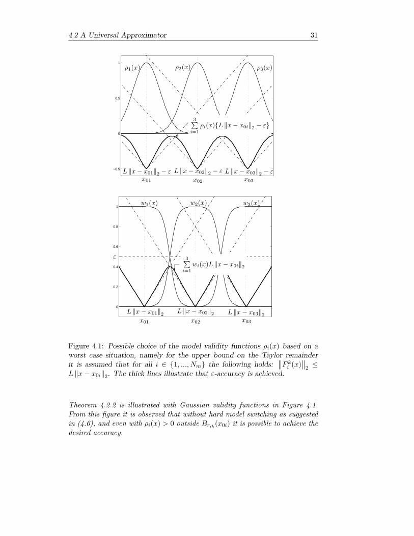
Figure 4.1: Possible choice of the model validity functions ρi(x) based on aworst case situation, namely for the upper bound on the Taylor remainderit is assumed that for all i ∈ 1, ..., Nm the following holds:
∥∥F ki (x)
∥∥2≤
L ‖x− x0i‖2. The thick lines illustrate that ε-accuracy is achieved.
Theorem 4.2.2 is illustrated with Gaussian validity functions in Figure 4.1.From this figure it is observed that without hard model switching as suggestedin (4.6), and even with ρi(x) > 0 outside Brik(x0i) it is possible to achieve thedesired accuracy.
32 Approximation
4.3 Upper bound on the Number of Models
Next an upper bound on the number of models Nm will be derived, that issufficient to construct a PLM with ε-accuracy. The upper bound is based ona worst case analysis, that means we use the fact that
‖f(x)− g(x)‖2 ≤Nm∑i=1
wi(x)Lik ‖x− x0i‖2 (4.9)
≤ L
Nm∑i=1
wi(x) ‖x− x0i‖2
where L ≥ Lik for all i ∈ 1, ..., Nm.We are faced with the problem of covering the region X with hyperballs
Br(x0i) = x | ‖x− x0i‖2 ≤ r = εL. Again it is assumed that X is a
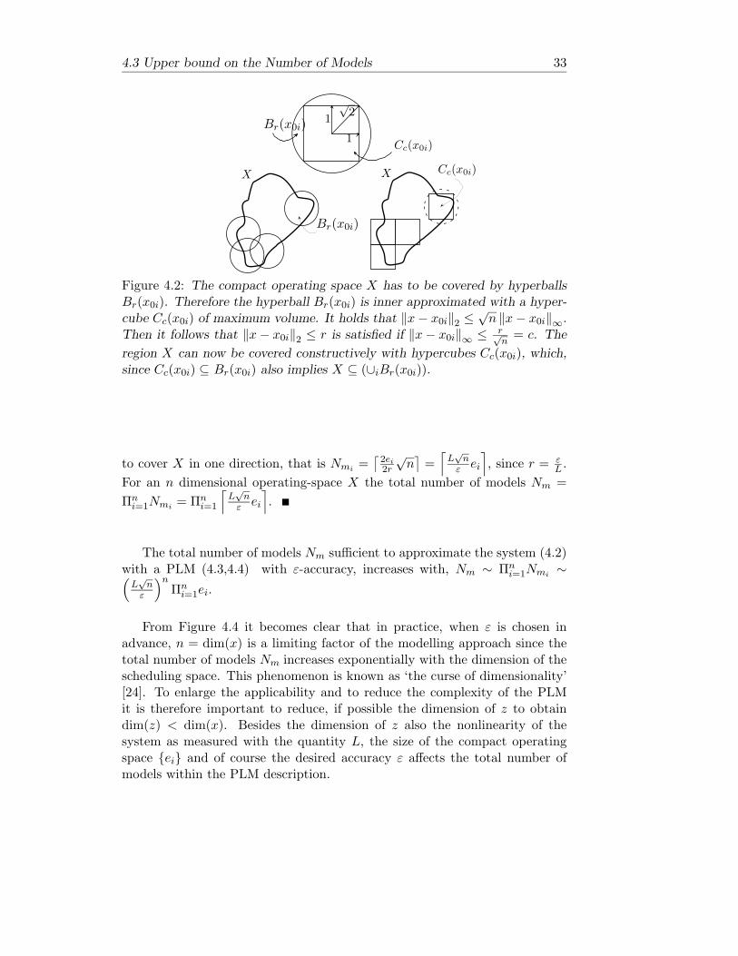
compact operating space, because then a finite number of models Nm sufficesto cover X. It is in general easier to cover X with hypercubes Cc(x0i) =x | ‖x− x0i‖∞ ≤ c where ‖v‖∞ = maxi |vi|. This leads to the followingidea. First inner-approximate the hyperball Br(x0i) with a hypercube Cc(x0i)of maximum volume. Then cover the region X with hypercubes Cc(x0i) toobtain the conditions the model has to satisfy to guarantee X ⊆ (∪iCc(x0i)),which, since Cc(x0i) ⊆ Br(x0i) also implies X ⊆ (∪iBr(x0i)). A graphicalinterpretation of the previous idea, for a two dimensional state space is givenin Figure 4.2. The radius of the circle Br(x0i) (hyperball) is r, the width of thesquare Cc(x0i) (hypercube) is 2c and the centre of Br(x0i) and Cc(x0i) is x0i.The working points x0i are uniformly distributed over the operating space asa result of the worst case analysis based on (4.9). The next result is based onthe hypercube partitioning of the operating space as illustrated in Figure 4.3.Here the operating space is (in each dimension) characterized with its centerdi and width ei as depicted in Figure 4.3.
Before stating the result we define the ceiling operator . : R → N+ thatmaps a real to the nearest integer towards infinity.
Theorem 4.3.1 Under the hypothesis of Theorem 4.2.2, given X = x ||xi − di| ≤ ei, i = 1, · · · , n, and ε > 0 arbitrary, it suffices to construct aPLM (4.3,4.4) with Nm = Πn
i=1
⌈L√n
ε ei
⌉, where L is from (4.9), to assure
that dfg(X) ≤ ε.
Proof. It holds that ‖x− x0i‖2 ≤√
n ‖x− x0i‖∞. Then it follows that‖x− x0i‖2 ≤ r is satisfied if ‖x− x0i‖∞ ≤ r√
n. This implies that to cover X
with hypercubes Cc(x0i) it is necessary that the width of the hypercubes isless or equal to 2r√
n. This leads to the number of models Nmi that is sufficient
4.3 Upper bound on the Number of Models 33
X X
Br(x0i)
Br(x0i)1
1√
2
Cc(x0i)
Cc(x0i)
Figure 4.2: The compact operating space X has to be covered by hyperballsBr(x0i). Therefore the hyperball Br(x0i) is inner approximated with a hyper-cube Cc(x0i) of maximum volume. It holds that ‖x− x0i‖2 ≤
√n ‖x− x0i‖∞.
Then it follows that ‖x− x0i‖2 ≤ r is satisfied if ‖x− x0i‖∞ ≤ r√n
= c. The
region X can now be covered constructively with hypercubes Cc(x0i), which,since Cc(x0i) ⊆ Br(x0i) also implies X ⊆ (∪iBr(x0i)).
to cover X in one direction, that is Nmi =⌈2ei2r
√n⌉
=⌈L√n
ε ei
⌉, since r = ε
L .For an n dimensional operating-space X the total number of models Nm =Πn
i=1Nmi = Πni=1
⌈L√n
ε ei
⌉.
The total number of models Nm sufficient to approximate the system (4.2)with a PLM (4.3,4.4) with ε-accuracy, increases with, Nm ∼ Πn
i=1Nmi ∼(L√n
ε
)nΠn
i=1ei.
From Figure 4.4 it becomes clear that in practice, when ε is chosen inadvance, n = dim(x) is a limiting factor of the modelling approach since thetotal number of models Nm increases exponentially with the dimension of thescheduling space. This phenomenon is known as ‘the curse of dimensionality’[24]. To enlarge the applicability and to reduce the complexity of the PLMit is therefore important to reduce, if possible the dimension of z to obtaindim(z) < dim(x). Besides the dimension of z also the nonlinearity of thesystem as measured with the quantity L, the size of the compact operatingspace ei and of course the desired accuracy ε affects the total number ofmodels within the PLM description.

34 Approximation
Cc(x0i)Cc(x0i)
Br(x0i)X
x1
x2
e1 e1d1
e2
e2
Figure 4.3: Covering of compact region X = x | |xi − di| ≤ ei, i = 1, · · · , nwith hyperballs Br(x0i). First the hyperballs Br(x0i) are inner approximatedwith hypercubes Cc(x0i) of maximum volume. Then X is covered easily withhypercubes Cc(x0i). This implies that since Br(x0i) covers Cc(x0i), also X iscovered with hyperballs Br(x0i) as desired.
0 1 2 3 4 50
10
20
30
40
50
60
Nm
n = dim(x) 0 1 2 3 4 5 6 7 8 9 100
10
20
30
40
50
60
70
80
90
100N
m
ε
0 1 2 3 4 5 6 7 8 9 100
1
2
3
4
5
6
7
8
9
10
Nm
ei = e 0 1 2 3 4 5 6 7 8 9 100
1
2
3
4
5
6
7
8
9
10
Nm
L
Figure 4.4: Dependence of Nm on relevant parameters Nm ∼(
L√n
ε
)nΠn
i=1ei.
4.4 Upper bound on the Difference between Trajec-tories
We will relate the ε-accuracy between the right-hand side of two systems tothe difference in solutions of the two systems.
With the bound dfg ≤ ε, that is the approximation error on the right-hand
4.5 Systems with Inputs 35
side of two systems, an upper bound on the difference between the trajectoriesof the system (4.2) and the PLM (4.3) will be derived. The result is in factbased on a variation on the Gronwall Lemma, see e.g. [67] and [79].
Theorem 4.4.1 Given the system (4.2) with f ∈ C1, and an approximatemodel (4.3), for instance a PLM, such that dfg(E) ≤ ε, then the solutionsξ(t) of (4.2) and ζ(t) of (4.3) starting at ξ(0) = ζ(0) that remain in E areuniformly close on the interval [0, T ] in the following sense:
‖ξ(t)− ζ(t)‖2 ≤ εeLt − 1
L(4.10)
where L is an upper bound on∥∥∥∂f∂x
∥∥∥2.
Proof. Note that ξ(t) = ξ(0)+∫ t0 f(ξ(τ))dτ and ζ(t) = ζ(0)+
∫ t0 g(ζ(τ))dτ
from which it follows that ξ(t)− ζ(τ) =∫ t0f(ξ(τ))− g(ζ(τ))dτ . If we write
f(ξ(τ))− g(ζ(τ)) = f(ξ(τ))− f(ζ(τ)) + f(ζ(τ))− g(ζ(τ)), and substitute thisin the integral equation, take norms and use the triangle inequality we have‖ξ(t)− ζ(t)‖2 ≤
∫ t0‖f(ξ(τ))− f(ζ(τ))‖2 + ‖f(ζ(τ))− g(ζ(τ))‖2dτ . Since f
is Lipschitz (in fact also C1), that is ‖f(ξ(τ))− f(ζ(τ))‖2 ≤ L ‖ξ(τ)− ζ(τ)‖2with L an upper bound on
∥∥∥∂f∂x
∥∥∥2, and supζ(τ)∈E ‖f(ζ(τ))− g(ζ(τ))‖2 ≤ ε it
is also true that
‖ξ(t)− ζ(t)‖2 ≤∫ t
0L ‖ξ(τ)− ζ(τ)‖2 dτ + εt (4.11)
Now define F (t) := e−Lt(∫ t0 L ‖ξ(τ)− ζ(τ)‖2 dτ − ∫ t
0 εLτe−L(t−τ)dτ) for allt ≥ 0. Taking the time derivative of F yields F (t) = Le−Lt(‖ξ(t)− ζ(t)‖2 −∫ t0 L ‖ξ(τ)− ζ(τ)‖2 dτ−εt) from which we can conclude that in order to satisfy
(4.11) for all t ≥ 0 we have F (t) = F (t) − F (0) =∫ t0 F (t)dτ ≤ 0. This
implies that∫ t0 L ‖ξ(τ)− ζ(τ)‖2 dτ ≤ ∫ t
0 εLτe−L(t−τ)dτ has to hold. With thisbound substituted in (4.11) we obtain ‖ξ(t)− ζ(t)‖2 ≤
∫ t0 εLτe−L(t−τ)dτ+εt =
ε eLt−1L .
The upper bound (4.10) will be useful if we analyze properties of trajecto-ries of systems, such as convergence, based upon an ε-accurate approximatemodel. This will become clear later on.
4.5 Systems with Inputs
The derived approximation results are easily extended to handle systems withinputs and outputs. For reason of clarity we will only consider the state
36 Approximation
equation of the system
x = f(x, u) (4.12)y = h(x, u) (4.13)
with state x ∈ X ⊆ Rn, input u ∈ U ⊆ R
m, and output y ∈ Y ⊆ Rp. The
objective is to approximate (4.12) with an ε-accurate approximate model
x = g(x, u) (4.14)
within a predefined compact region Ψ ⊆ X × U . Since our main interest is inPLMs, we specialize to models with right-hand side
g(x, u) =Nm∑i=1
wi(x, u)gi(x, u) (4.15)
where
gi(x, u) = Aix + Biu + ai
In that case the locally valid models, the k−th order Taylor series expansionsof the system, are scheduled on the n + m dimensional operating space Ψ toobtain an ε-accurate PLM. In particular, the following application of Theorem4.2.2 and Theorem 4.3.1 will be a useful approximation result for systems withinputs.
Corollary 4.5.1 Given f(ψ) ∈ C2(Ψ) the right-hand side of the state equa-tion of (4.12) with Ψ = ψ | |ψi − di| ≤ ei, i = 1, · · · , n + m, and ε > 0 arbi-
trary. There exists a right-hand side of a PLM, that is g(ψ) =Nm∑i=1
wi(ψ)gi(ψ),
with Nm = Πn+mi=1
⌈ei√2ε
√λξn1/2(n + m)
⌉finite such that dfg(Ψ) ≤ ε.
Proof. Firstly, it is assumed that f(x, u) is C2, that means at least 2times continuously differentiable with respect to x and u. This allows us todecompose the right-hand side of the state equation of (4.12) as follows
f(x, u) = fpi (x, u) + F p
i (x, u)
with 0 ≤ p ≤ 2 and fpi (x, u) a p-th order Taylor series expansion of f around
ψ0i = (x0i, u0i), and F pi (x, u) := f(x, u) − fp
i (x, u) is defined as the corre-sponding Taylor remainder. Since PLMs consist of (nonhomogeneous) linearmodels, we take p = 1. Application of the Mean Value Theorem allows us torewrite the j-th component of vector F 1
i (ψ) as
F 1i,j(ψ) =
12[ψ − ψ0i]T
∂2fj∂ψ2
(ξi)[ψ − ψ0i]

4.5 Systems with Inputs 37
here ψ = [xT uT ]T , ψ0i = [xT0i uT
0i]T and the matrix ∂2fj
∂ψ2 (ξi) =[
∂2fj∂ψp∂ψq
(ξi)]
with ξi ∈ [ψ0i, ψ]. It is assumed that the triples (Ai, Bi, ai) that specify thelinear models gi(ψ) from the PLM (4.14,4.15) are chosen as Taylor lineariza-tions of f(ψ) in the points ψ0i, that is gi(ψ) = f1
i (ψ) from (4.15). In thatcase the triples become (∂f∂x (x0i, u0i),
∂f∂u(x0i, u0i), f (x0i, u0i)− ∂f
∂x (x0i, u0i)x0i−∂f∂u(x0i, u0i)u0i) and for the difference between the system and the PLM wehave
f(ψ)−Nm∑i=1
wi(ψ)f1i (ψ) =
Nm∑i=1
wi(ψ)(f(ψ)− f1i (ψ))
=Nm∑i=1
wi(ψ)F 1i (ψ) (4.16)
With ri = ψ − ψ0i we obtain
F 1i (ψ) =
12[rTi
∂2f1∂ψ2
(ξi)ri · · · rTi∂2fn∂ψ2
(ξi)ri]T (4.17)
Then the following upper bound for the contribution of model gi = f1i to the
approximation error can be derived
∥∥F 1i (ψ)
∥∥2≤ 1
2(
n∑j=1
λ2j,ξi(rTi ri)2)1/2
≤ 12√
nλξi ‖ψ − ψ0i‖22 (4.18)
with
λj,ξi = maxξi∣∣∣∣eig(∂2fj
∂ψ2(ξi))
∣∣∣∣λξi = max
jλj,ξi
The upper bound is conservative since by taking the maximum it is assumedthat the maximum nonlinearity (as measured with the maximum absoluteeigenvalue of the Hessian matrices associated with the Taylor remainder) canoccur in every scalar equation of the set of equations, see (4.12). With thenorm bound of the second order term as given in (4.18) it follows from (4.16)that:
‖f(ψ)− g(ψ)‖2 ≤Nm∑i=1
wi(ψ)12√
nλξi ‖ψ − ψ0i‖22 (4.19)
38 Approximation
The approximation error is smaller than ε if
Nm∑i=1
wi(ψ)12√
nλξi ‖ψ − ψ0i‖22 ≤ ε ∀ψ ∈ Ψ (4.20)
Rearranging the terms in (4.20) yields
Nm∑i=1
ρi(ψ)λξi ‖ψ − ψ0i‖22 −2ε√
n ≤ 0 ∀ψ ∈ Ψ (4.21)
If we substitute λξ = maxλξi for λξi, which means that the maximumnonlinearity can occur everywhere within the operating space, one obtains
Nm∑i=1
ρi(ψ)λξ ‖ψ − ψ0i‖22 −2ε√
n ≤ 0 ∀ψ ∈ Ψ (4.22)
This condition can be satisfied for finite Nm within a compact set, that is ifΨ ⊆ (∪i∈INmBr(ψ0i)) with radius r =
√2ε√nλξ
. This is just an application
of Theorem 4.2.2. Now by application of Theorem 4.3.1 and given Ψ = ψ ||ψi − di| ≤ ei, i = 1, · · · , n + m it follows that it suffices to construct a PLMwith Nm = Πn+m
i=1
⌈eir
√n + m
⌉= Πn+m
i=1
⌈ei√2ε
√λξ√
n(n + m)⌉
to assure thatdfg(Ψ) ≤ ε.
Example 4.5.2 Consider the following application of Corollary 4.5.1. Theobjective is to approximate the system
x = f(x, u) = x2 + xu (4.23)
with a PLM
x = g(x, u) =Nm∑i=1
wi(x, u)gi(x, u)
where
gi(x, u) = Aix + Biu + ai
such that dfg(Ψ) ≤ 1 for Ψ = (x, u) | |x| ≤ 2, |u| ≤ 1. The right-hand sideof (4.23) can be rewritten as
f(x, u) = f1i (x, u) + F 1
i (x, u)

4.5 Systems with Inputs 39
with the first order Taylor series
f1i (x, u) = f (x0i, u0i) +
∂f
∂x(x0i, u0i)(x− x0i) +
∂f
∂u(x0i, u0i)(u− u0i)
= −x20i − x0iu0i + (2x0i + u0i)x + x0iu
and the corresponding Taylor remainder
F 1i (x, u) := f(x, u)− f1
i (x, u) =12[
x− x0i u− u0i] ∂2f
∂ψ2
[x− x0iu− u0i
]
where ∂2f∂ψ2 =
[2 11 0
]. We obtain for λξ = max
∣∣∣∣eig([
2 11 0
])∣∣∣∣ = 1 +
√2.
Then to achieve ε-accuracy, it suffices to construct a PLM with Nm models,where
Nm =⌈
2√2
√2.41 ∗ 2
⌉∗⌈
1√2
√2.41 ∗ 2
⌉= 4 ∗ 2 = 8
The operating points (x0i, u0j) with i ∈ 1, 2, 3, 4 and j ∈ 1, 2 are chosenequidistantly since the upper bound for the number of models is based on aworst case scenario, namely the maximum nonlinearity as measured with thebound on the Taylor remainder can occur at every place in the operating space.The corresponding triples defining the polytopic model are
(Ai, Bi, ai) = (2x0i + u0j , x0i,−x20i − x0iu0j)
with centers at
(x01, x02, x03, x04) = (−1.5,−0.5, 0.5, 1.5)(u01, u02) = (−0.5, 0.5)
uniformly distributed over the operating space, see Figure 4.5.The model validity functions are chosen Gaussian functions, namely
ρi(ψ) = e−7(ψ−ψ0i)T (ψ−ψ0i)
With the objective dfg(Ψ) ≤ ε, model validity is made precise, meaning that theoperating regimes Ψi are naturally induced by means of the local model validityregions Br(x0i). The operating regimes are constructed such that Ψi ⊆ Br(x0i)and Ψ ⊆ ∪i∈1,...,NmΨi.

40 Approximation
−1
−0.5
0
0.5
1
−2
−1
0
1
2−1
0
1
2
3
4
5
6
x u
f(x,u)
−1
−0.5
0
0.5
1
−2
−1
0
1
20
0.2
0.4
0.6
0.8
1
x u
ρi(x,u)
−1
−0.5
0
0.5
1
−2
−1
0
1
2−2
−1
0
1
2
3
4
5
6
x u
g(x,u)
and
‖f(x,u)−g(x,u)‖
2
−1
−0.5
0
0.5
1
−2
−1
0
1
20
0.2
0.4
0.6
0.8
1
x u
wi(x,u)
Figure 4.5: System and ε-accurate PLM constructed as suggested in Corollary4.5.1. Uniform distribution of the scheduling regimes Zi over the schedulingspace which equals the operating space, that is Z = Ψ.
4.6 Systems with Structure
When the operating space is high dimensional, the ‘curse of dimensionality’will restrict the applicability of the polytopic linear modelling approach. Thecore of this problem is that the number of operating regimes needed to uni-formly partition the operating space increases exponentially with the dimen-sion of the operating space, see Theorem 4.3.1 and Figure 4.4. Uniform parti-tioning is often not necessary (as will become clear later on), but the problemis still significant. However, in some cases the models can be scheduled on aspace of lower dimension, which will reduce the curse of dimensionality consid-erably. On the basis of the approximation results that where derived earlier,a suitable choice of variables z = s(ψ), that constitute the scheduling space,will be determined and defined. A situation in which dim(z) can be chosensmaller than dim(ψ) is illustrated in the next example.
Example 4.6.1 Consider the system
x1 = x2
x2 = 3x1 + x22

4.6 Systems with Structure 41
which has two important features that restrict the upper bound (4.18) in astructural way. First, one of the two scalar differential equations with right-hand side fi(ψ) is linear, and secondly only x2 appears nonlinear in this systemdescription. As a result we take z = x2, because all other variables, in thiscase only x1, appear linear in fi(ψ). In this case
∂2f1∂ψ2
(ξ) =[
0 00 0
]∂2f2∂ψ2
(ξ) =[
0 00 2
]
The Taylor remainder is
F 1(ψ) =12
[ψ − ψ0i]T[
0 00 0
][ψ − ψ0i]
[ψ − ψ0i]T[
0 00 2
][ψ − ψ0i]
=[
0(x2 − x20)
2
]
and depends only on x2 since the system is linear in x1. The Taylor remaindermeasures the nonlinearity of the system. In this case
∥∥F 1(ψ)∥∥2≤ 1
2√
nλξi ‖z − z0i‖22 (4.24)
with z = x2. Moreover when there are linear differential equations fj(ψ),like f1(ψ), we can further reduce conservatism of the upper bound (4.18) byreplacing it with
∥∥F 1(ψ)∥∥2≤ 1
2√
nNλξi ‖z − z0i‖22 (4.25)
where nN is the number of nonlinear differential equations fj(ψ).
The example shows that the upper bound on the approximation error(4.25) compared with (4.18) can be significantly reduced if the system showssome structural properties that can be exploited, e.g. linearity of the systemwith respect to some variables. In this section the objective is to reveal some ofthese structural properties. From the preceding example and the applicationof Theorem 4.2.2 and Theorem 4.3.1 we have the following result concerningthe reduction of the operating space.
Corollary 4.6.2 Given f(ψ) = FψL + f1(ψN ) with f1(ψN ) ∈ C2(E), Ean open subset of R
nZ where ψL ∈ ΨL, ψN ∈ ΨN , and ΨL × ΨN = Ψ and
42 Approximation
f1 : ΨN → Rn is a nonlinear n-dimensional vector valued function with n−nN
scalar linear components and F ∈ Rn×dim(ψL), and ε > 0 arbitrary. Withinany set Ψ, with ΨN compact such that ΨN ⊂ E there exists a right-hand sideof a PLM, with z = ψN , that is g(ψ) =
∑Nmi=1 wi(z)gi(ψ) with Nm finite such
that dfg(Ψ) ≤ ε. Moreover given ΨN = Z = z | |zi − di| ≤ ei, i = 1, · · · , nZ,it suffices to construct a PLM (4.14,4.15) with Nm = Πnz
i=1
⌈ei√2ε
√λξn
1/2N nz
⌉.
Proof. Define gi(ψ) := FψL+f11i(ψN ). Then it follows that f(ψ)−g(ψ) =∑Nm
i=1 wi(z)f1(ψN ) − f11i(ψN ). Corollary 4.5.1 can now be applied, which
shows that if ΨN is compact and with z = ψN a finite number of models
Nm = Πnzi=1
⌈ei√2ε
√λξn
1/2N nz
⌉is sufficient to achieve ε-accuracy.
It is shown that the operating vector z must be chosen such that it capturesthe system’s nonlinearities.
Another structure that appears often in practice, are so-called affine right-hand sides of systems:
f (ψ) = f (ψL, ψN ) = f1 (ψN ) + f2 (ψN )ψL (4.26)
where ψL ∈ ΨL, ψN ∈ ΨN , and ΨL × ΨN = Ψ. Furthermore f1 : ΨN → Rn
and f2 : ΨN → Rn×dim(ψL) are nonlinear vector- and matrix-valued functions,respectively. As an example, models of mechanical systems are often affinein the input [57]. For the right-hand side of the state equation of such amechanical system it holds that ψN = x, the state, and ψL = u, the input. Itwill be the objective to approximate (4.26) with a PLM
g (ψ) =Nm∑i=1
wi(z)gi(ψ) (4.27)
where
gi(ψ) = A∗i ψ + a∗i
and where z = s(ψ).
Theorem 4.6.3 Assume fi ∈ C1(E) as given by (4.26), Ψ = ψ | |ψi − di| ≤ei, i = 1, · · · , n + m, and ε > 0 arbitrary. It suffices to choose z = ψN
from (4.27) such that dfg(Ψ) ≤ ε. Furthermore if fi ∈ C2(E) it suffices toconstruct a PLM with Nm = ΠnZ
i=1Nmi models to assure that dfg(Ψ) ≤ ε.
HereNmi =⌈2ei2rk
√nZ
⌉the number of models in direction i, nZ equals the

4.6 Systems with Structure 43
dimension of z, and
rk =
r1 = ε
λ1/2ξ,2 ‖ψL‖2
(−λξ,2‖ψL‖2
2√nλξ,1ε
+√
2λξ,2‖ψL‖22√
nλξ,1ε+
λ2ξ,2‖ψL‖4
2
nλ2ξ,1ε
2
)if g(ψ) =
∑Nmi=1 wi(ψN )gi(ψ)
r0 = ε
1
λ1/2ξ,1
λ1/2ξ,2 ‖ψL‖2
1
λ1/2ξ,1
+ 1
λ1/2ξ,2 ‖ψL‖2
if g(ψ) =∑Nm
i=1 wi(ψN )gi(ψL)(4.28)
Proof. Fix an arbitrary ψ = (ψL, ψN ) ∈ Ψ = ΨL ×ΨN . Then
f (ψ)− g (ψ) = f (ψN , ψL)−Nm∑i=1
wi (ψN ) gi(ψN , ψL)
=Nm∑i=1
wi (ψN ) f1(ψN ) + f2(ψN )ψL − gi(ψN , ψL)
=Nm∑i=1
wi (ψN ) f1(ψN )− gi1(ψN ) + f2(ψN )ψL − gi2(ψL)
In the last line we split the linear function gi : Ψ→ Rn into two linear functionsgi1 : ΨN → Rn and gi2 : ΨL → Rn, that is gi(ψ) = gi1(ψN ) + gi2(ψL). Withgi2(ψL) = ΓiψL, where Γi is a not yet specified constant parameter matrix.Then we have
‖f (ψ)− g (ψ)‖2
=
∥∥∥∥∥Nm∑i=1
wi (ψN ) f1(ψN )− gi1(ψN ) + (f2(ψN )− Γi)ψL∥∥∥∥∥2
≤∥∥∥∥∥Nm∑i=1
wi (ψN ) f1(ψN )− gi1(ψN )∥∥∥∥∥2
+
∥∥∥∥∥Nm∑i=1
wi (ψN ) f2(ψN )− ΓiψL
∥∥∥∥∥2
≤∥∥∥∥∥f1(ψN )−
Nm∑i=1
wi (ψN ) gi1(ψN )
∥∥∥∥∥2
+ ‖ψL‖2∥∥∥∥∥f2(ψN )−
Nm∑i=1
wi (ψN ) Γi
∥∥∥∥∥2
44 Approximation
By application of Theorem 4.2.2 the first and the second term can be madearbitrarily small with a finite number of models. There is some freedom left.The first term can be made arbitrarily small by choosing gi1 = fk
1i with k ∈0, 1, that is a zero-th or first order Taylor series expansion of f1(ψN ) aroundψN0i. The case that k = 0, the function gi(ψ) = gi1(ψN0i) + gi2(ψL) = gi(ψL)otherwise gi(ψ) = gi1(ψN ) + gi2(ψL) = gi(ψN , ψL).
Following the analysis as presented in Section 4 we determine the numberof models Nm, and the model parameters from the PLM description neededto approximate (4.26) within the region Ψ with ε-accuracy.
First consider the case k = 1, where we assume f1(ψN ) to be C2, then
f1(ψN ) = f1(ψN0i) +∂f1∂ψN
(ψN0i)(ψN − ψN0i) (4.29)
+ F 11i(ψN )
The last term of (4.29) is the Taylor remainder. Application of the MeanValue Theorem allows us to rewrite the j-th component of F 1
1i(ψN ) as
F 11i,j(ψ) =
12[ψN − ψN0i]T
∂2f1j∂ψ2
N
(ξi)[ψN − ψN0i]
here the matrix ∂2f1j
∂ψ2 (ξi) =[
∂2f1j
∂ψNp∂ψNq(ξi)
]with ξi ∈ [ψN0i, ψN ]. If we assume
that f2(ψN ) is at least one time differentiable, then we obtain for
f2(ψN ) = f2(ψN0i) (4.30)+ F 0
2i(ψN )
The last term of (4.30) is the Taylor remainder. Application of the MeanValue Theorem allows us to rewrite F 0
2i(ψN ) as
F 02i(ψN ) =
∂f2∂ψN
(ξi)(ψN − ψN0i)
with ξi ∈ [ψN0i, ψN ]. We will approximate with a desired accuracy the affinesystem (4.26) in a predefined region Ψ with a PLM
x = g(ψ) (4.31)
=Nm∑i=1
wi(ψN )f1(ψN0i) +∂f1∂ψN
(ψN0i)(ψN − ψN0i) + f2(ψN0i)ψL(4.32)
4.6 Systems with Structure 45
The difference between the system and the PLM becomes
f(ψ)− g(ψ) =Nm∑i=1
wi(ψN )F 11i(ψN )
+Nm∑i=1
wi(ψN )F 02i(ψN )ψL (4.33)
We split the Euclidean norm of (4.33) in two parts. The first and the secondpart are respectively the Euclidean norm of the first and the second term of(4.33). We can write
‖f(ψ)− g(ψ)‖2 ≤ ε
≤ ε1 + ε2
with ∥∥∥∥∥Nm∑i=1
wi(ψN )F 11i(ψN )
∥∥∥∥∥2
≤ ε1 (4.34)
∥∥∥∥∥Nm∑i=1
wi(ψN )F 02i(ψN )ψL
∥∥∥∥∥2
≤ ε2 (4.35)
We observe that (4.34) is similar to (4.16). This leads to a condition equivalentto (4.20):
Nm∑i=1
wi(ψN )1/2√
nλξ,1 ‖ψN − ψN0i‖22 ≤ ε1 (4.36)
where
λξ,1 = maxi
max
j
maxξi
∣∣∣∣eig(∂2f1j∂ψ2
(ξi))∣∣∣∣
We obtain∥∥∥∥ ∂f2∂ψN
(ξi)(ψN − ψN0i)∥∥∥∥2
≤ λ1/2ξi,2 ‖ψN − ψN0i‖2 (4.37)
where
λξi,2 = maxξi∣∣∣∣eig( ∂f2
∂ψN(ξi)T
∂f2∂ψN
(ξi))∣∣∣∣
46 Approximation
Then, with the norm given in (4.37) we obtain for (4.35)
Nm∑i=1
wi(ψN )λ1/2ξ,2 ‖ψN − ψN0i‖2 ‖ψL‖2 ≤ ε2 (4.38)
where
λξ,2 = maxi
λξi,2
Now the question is how to choose ε1 and ε2 of (4.36) and (4.38) such that wecan guaranty ‖f(ψ)− g(ψ)‖2 ≤ ε. We substitute
ε1 = αε (4.39)ε2 = (1− α)ε (4.40)
where
α ∈ (0, 1)
With (4.39) and (4.40) we obtain ε1 + ε2 = ε. Rearranging (4.36) and (4.38)and substituting (4.39) and (4.40) gives
Nm∑i=1
ρi(ψN )(‖ψN − ψN0i‖22 −
2εα√nλξ,1
)≤ 0 ∀ψ ∈ Ψ (4.41)
Nm∑i=1
ρi(ψN )
‖ψN − ψN0i‖2 −
ε (1− α)
λ1/2ξ,2 ‖ψL‖2
≤ 0 ∀ψ ∈ Ψ (4.42)
The upper bound on the number of models, that is Nm, is determined bythe minimum of r1(α) =
√2εα√nλξ,1
and r2(α) = ε(1−α)
λ1/2ξ,2 ‖ψL‖2
, since both (4.41)
and (4.42) have to be satisfied. To construct a PLM with Nm as small aspossible, α has to be computed as the one that maximizes min(r1(α), r2(α)),that is α∗ = argmaxα∈(0,1) min(r1(α), r2(α)). If we assume that there existsan α∗ ∈ (0, 1) such that r1(α∗) = r2(α∗) then for any nonzero perturbation δαsuch that α∗ + δα ∈ [0, 1] the following holds min(r1(α∗), r2(α∗)) = r1(α∗) =r2(α∗) > maxδα =0|α∗+δα∈[0,1] min(r1(α∗+δα), r2(α∗+δα)). This can be veryeasily seen since for any nonzero perturbation δα of α∗ as suggested, eitherr1(α∗+δα) < r1(α∗) or r2(α∗+δα) < r2(α∗) and thus min(r1(α∗+δα), r2(α∗+δα)) is smaller then min(r1(α∗), r2(α∗)) which implies that a∗ is the uniquemaximizer. Next it will be shown that there always exists an α∗ ∈ (0, 1).Therefore we set
r = r1(α) = r2(α) =
√2εα√nNλξ,1
=ε (1− α)
λ1/2ξ,2 ‖ψL‖2
(4.43)
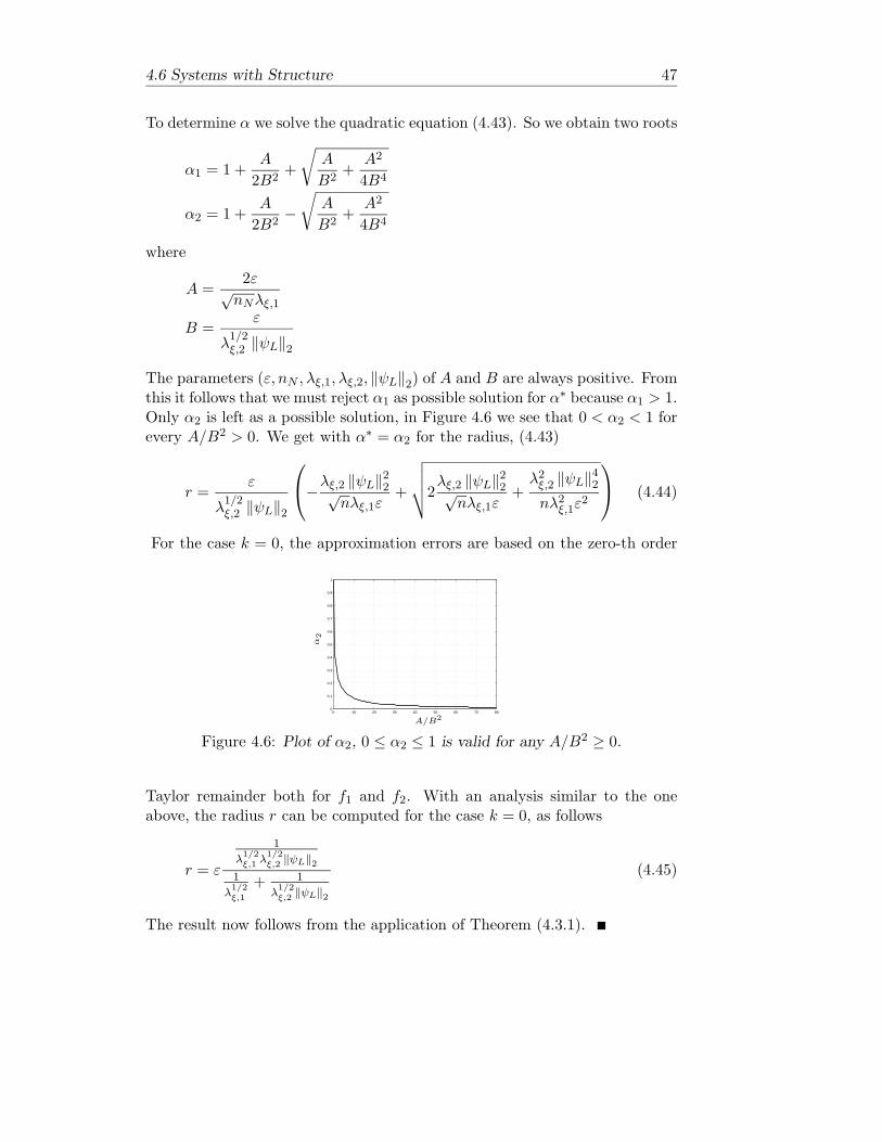
4.6 Systems with Structure 47
To determine α we solve the quadratic equation (4.43). So we obtain two roots
α1 = 1 +A
2B2+
√A
B2+
A2
4B4
α2 = 1 +A
2B2−√
A
B2+
A2
4B4
where
A =2ε√
nNλξ,1
B =ε
λ1/2ξ,2 ‖ψL‖2
The parameters (ε, nN , λξ,1, λξ,2, ‖ψL‖2) of A and B are always positive. Fromthis it follows that we must reject α1 as possible solution for α∗ because α1 > 1.Only α2 is left as a possible solution, in Figure 4.6 we see that 0 < α2 < 1 forevery A/B2 > 0. We get with α∗ = α2 for the radius, (4.43)
r =ε
λ1/2ξ,2 ‖ψL‖2
−λξ,2 ‖ψL‖22√
nλξ,1ε+
√√√√2λξ,2 ‖ψL‖22√
nλξ,1ε+
λ2ξ,2 ‖ψL‖42nλ2ξ,1ε
2
(4.44)
For the case k = 0, the approximation errors are based on the zero-th order
0 10 20 30 40 50 60 70 800
0.1
0.2
0.3
0.4
0.5
0.6
0.7
0.8
0.9
1
A/B2
α2
Figure 4.6: Plot of α2, 0 ≤ α2 ≤ 1 is valid for any A/B2 ≥ 0.
Taylor remainder both for f1 and f2. With an analysis similar to the oneabove, the radius r can be computed for the case k = 0, as follows
r = ε
1
λ1/2ξ,1 λ
1/2ξ,2 ‖ψL‖2
1
λ1/2ξ,1
+ 1
λ1/2ξ,2 ‖ψL‖2
(4.45)
The result now follows from the application of Theorem (4.3.1).
48 Approximation
The result is illustrated by means of two examples. It is clear that thecurse of dimensionality can not be avoided, but the reduction in dimensionconsiderably reduces this problem for a significant number of modelling prob-lems, as we shall illustrate with these examples. The first example shows thecase that rk = r1. The second example illustrates the case that rk = r0.
Example 4.6.4 Consider the following application of Theorem 4.6.3 for thecase k = 1. The objective is to approximate the system
x = f(x, u) = x2 + xu (4.46)
with a PLM
x = g(x, u) =Nm∑i=1
wi(x)gi(x, u)
where
gi(x, u) = Aix + Biu + ai
such that dfg(Ψ) ≤ 1 for Ψ = (x, u) | |x| ≤ 2, |u| ≤ 1. The right-hand sideof (4.46) can be rewritten as follows
f(x, u) = f1(x) + f2(x)u
with
f1(x) = x2 (4.47)f2(x) = x (4.48)
Rewrite (4.47) as follows
f1(x) = f11i(x) + F 1
1i(x)
with the first order Taylor series
f11i(x) = f1(x0i) +
∂f1∂x
(x0i)(x− x0i)
= −x2 + 2x0ix
and the corresponding Taylor remainder
F 11i(x) := f1(x)− f1
1i(x) =12
∂2f1∂x2
(x− x0i)2
4.6 Systems with Structure 49
where ∂2f1
∂x2 = 2. We obtain λξ,1 = 2. Next rewrite (4.48) as follows
f2 (x) = f02i(x) + F 0
2i(x)
with the zero-th order Taylor series
f02i(x) = f2(x0i)
= x0i
and the corresponding Taylor remainder
F 12i(x) := f2(x)− f0
2i(x) =∂f2∂x
(x− x0i)
where ∂f2
∂x = 1. We obtain λξ,2 = 1. We find for the radius (4.28) r1 = 0.618.Then it suffices to construct a PLM with Nm models, where
Nm =⌈
20.618
√1⌉
= 4
Given that the operating regimes are uniformly distributed over the operatingspace we find for the centres of the operating regimes
(x01, x02, x03, x04) = (−1.5,−0.5, 0.5, 1.5)
The corresponding triples defining the polytopic model are
(Ai, Bi, ai) = (2x0i, x0i,−x20i)
see Figure 4.7. The model validity functions are chosen
ρi(x) =1
2 ‖x− x0i‖22Compared to Example 4.5.2 the scheduling space is reduced. The result is a re-duction of local model parameters by a factor two, that is 12 model parametersnow against 24 for Example 4.5.2.
An important practical application of the approximation result, Theorem4.2.2, for the case k = 0, is that it is always possible to eliminate dependenceof the locally valid models on the variables z, at least if Ψ is compact. Thiswas also shown in Theorem 4.2.2 and Theorem 4.6.3, and will be illustratedin the next example.
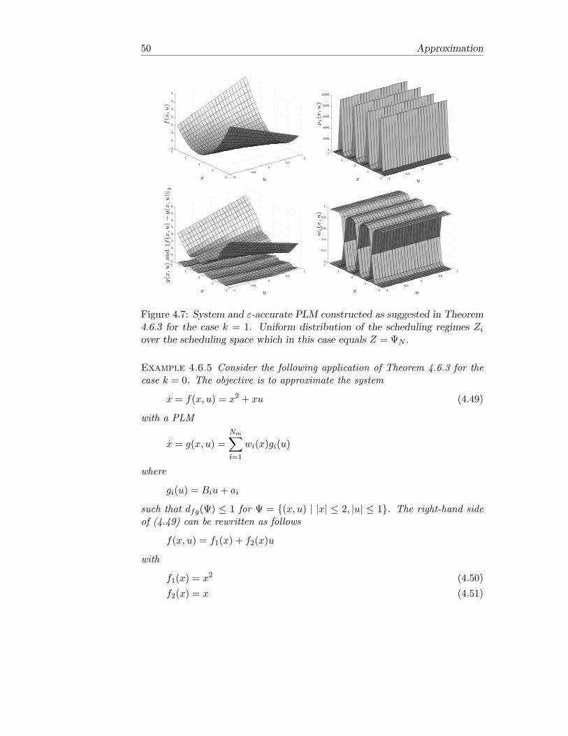
50 Approximation
−1
−0.5
0
0.5
1
−2
−1
0
1
2−1
0
1
2
3
4
5
6
x u
f(x,u)
−1
−0.5
0
0.5
1
−2
−1
0
1
20
2000
4000
6000
8000
10000
x u
ρi(x,u)
−1
−0.5
0
0.5
1
−2
−1
0
1
2−2
−1
0
1
2
3
4
5
6
x u
g(x,u)
and
‖f(x,u)−g(x,u)‖
2
−1
−0.5
0
0.5
1
−2
−1
0
1
20
0.2
0.4
0.6
0.8
1
x u
wi(x,u)
Figure 4.7: System and ε-accurate PLM constructed as suggested in Theorem4.6.3 for the case k = 1. Uniform distribution of the scheduling regimes Zi
over the scheduling space which in this case equals Z = ΨN .
Example 4.6.5 Consider the following application of Theorem 4.6.3 for thecase k = 0. The objective is to approximate the system
x = f(x, u) = x2 + xu (4.49)
with a PLM
x = g(x, u) =Nm∑i=1
wi(x)gi(u)
where
gi(u) = Biu + ai
such that dfg(Ψ) ≤ 1 for Ψ = (x, u) | |x| ≤ 2, |u| ≤ 1. The right-hand sideof (4.49) can be rewritten as follows
f(x, u) = f1(x) + f2(x)u
with
f1(x) = x2 (4.50)f2(x) = x (4.51)

4.6 Systems with Structure 51
Rewrite (4.50) as follows
f1(x) = f01i(x) + F 0
1i(x)
with the zeroth order Taylor series
f01i(x) = f1(x0i)
= x20i
and the corresponding Taylor remainder
F 01i(x) := f1(x)− f0
1i(x) =∂f1∂x
(ξ)(x− x0i)
where∣∣∣∂f1
∂x
∣∣∣ ≤ |x + x0i| = 4. We obtain λξ,1 = 4. Next rewrite (4.51) asfollows
f2 (x) = f02i(x) + F 0
2i(x)
with the zero-th order Taylor series
f02i(x) = f2(x0i)
= x0i
and the corresponding Taylor remainder
F 12i(x) := f2(x)− f0
2i(x) =∂f2∂x
(x− x0i)
where ∂f2
∂x = 1. We obtain λξ,2 = 1. We find for the radius (4.28) r1 = 0.2.Then it suffices to construct a PLM with Nm models, where
Nm =⌈
20.2
√1⌉
= 10
Given that the operating regimes are uniformly distributed over the operatingspace we find for the centres of the operating regimes
(x01, x02, ..., x09, x010) = (−1.8,−1.4, ..., 1.4, 1.8)
The corresponding triples defining the polytopic model are
(Ai, Bi, ai) = (0, x0i, x20i)
see Figure 4.8. Note that in this case the PLM description consists of 10∗2 =20 model parameters (of course not taken into account the 10 structural zeros).In the case of Example 4.6.4 there were 12 model parameters. The modelvalidity functions are chosen
ρi(x) =
1 if 4 ‖x− x0i‖2 − ε ≤ 00 if 4 ‖x− x0i‖2 − ε > 0

52 Approximation
−1
−0.5
0
0.5
1
−2
−1
0
1
2−1
0
1
2
3
4
5
6
x u
f(x
,u)
−1
−0.5
0
0.5
1
−2
−1
0
1
20
0.2
0.4
0.6
0.8
1
x u
ρi(
x,u
)
−1
−0.5
0
0.5
1
−2
−1
0
1
2−2
−1
0
1
2
3
4
5
6
x ug(x
,u)an
d‖f
(x,u
)−
g(x
,u)‖
2
−1
−0.5
0
0.5
1
−2
−1
0
1
20
0.2
0.4
0.6
0.8
1
x u
wi(
x,u
)Figure 4.8: System and ε-accurate PLM constructed as suggested in Theorem4.6.3 for the case k = 0. Uniform distribution of the scheduling regimes Zi
over the scheduling space which in this case equals Z = ΨN .
4.7 Notes and Comments
A universal approximator
We have shown that the right-hand side of a Ck (k ∈ 1, 2) ordinary differ-ential equation that describes the real system can be uniformly approximatedto an arbitrary accuracy ε on any compact operating space with a PLM, bymaking the decomposition into operating regimes sufficiently fine. Sometimesalso systems defined on an unbounded operating space can be approximated toan arbitrary accuracy ε with a finite number of operating regimes. The ideais to use a one to one coordinate transformation that maps the unboundedoperating space into a compact operating space. In the new coordinates thederived results can be applied. More on how the one to one mapping may beconstructed can be found in [83].
Systems with structure
We have seen that system structure, as presented by Corollary 4.6.2 and The-orem 4.6.3, can reduce the dimension of the operating space and thereby com-plexity of the model. Of course, the structures that we have analyzed and for
4.7 Notes and Comments 53
which model reduction, in the sense as described before was possible, dependson the choice of coordinates for the system. Stated otherwise, the distance dfg
that we have used and system structure as we have analyzed are not invariantunder coordinate transformations. Therefore it could be useful to search forcoordinate transformations, in such a way, that within the new coordinates thesystem can be approximated with a PLM consisting of fewer parameters, with-out affecting the approximation accuracy. One can think of transformationsthat transform the system to one of the proposed structures in this section.
More formally the question is under which conditions do there exist, andhow can we find, a nonsingular coordinate transformation
x = T−1(x)
such that within the new coordinates x the system (4.2)
.x = f(x)
can be approximated with a PLM (4.3)
.x = g(x)
in such a way that dfg(X) ≤ ε is achieved, and in such a way that the PLMg(x) consists of less models and/or parameters then g(x), the PLM obtainedfor the untransformed system. Since f(x) − g(x) = ∂T (x)
∂x
(f(x)− g(x)
), it
follows that dfg ≤ ε holds if∥∥∥∂T (x)
∂x
∥∥∥2
∥∥∥f(x)− g(x)∥∥∥2≤ ε or equivalently
(df g(X) ≤ ε)⇒ (dfg(X) ≤ ε)
where ε = ε∥∥∥ ∂T (x)∂x
∥∥∥2
and X = T (X).
It is imaginable that within the new coordinates x, the transformed systemf(x) exhibits some desired system structure in contrast to the untransformedsystem f(x), that could reduce ‘the curse of dimensionality’ and thereforereduce the upper bound Nm. It is conceivable however, that the state trans-formation comes at the expense of a reduced accuracy margin, ε∗ < ε andan increased operating region X > X, that has to be covered by Nm mod-els. It seems natural to search for transformations that reduce dim(z), sinceNm increases inverse proportional with at most
√ε, while Nm increases expo-
nentially with dim(z). Also state transformations that transform a set of nfirst-order nonlinear differential equations into n−nN first-order linear differ-ential equations together with nN nonlinear first order differential equations

54 Approximation
could considerably reduce the number of PLM parameters, at least if the con-tribution of
∥∥∥∂T (x)∂x
∥∥∥2, λξ,x, and X is of less importance2. A more detailed
treatment of simplifying state transformations is not the subject of this thesis,however.
2Note that under observability conditions it is always possible to find locally such statetransformations [57].

Chapter 5
Stability, Controllability andObservability by Duality
5.1 Introduction
In the previous chapters, the PLM structure was introduced as a candidatemodel structure for modeling a class of nonlinear systems, and was shownto be flexible. From an approximation point of view, every other universalapproximator could equally well be chosen, e.g. a polynomial or radial ba-sis function expansion or a neural network [24], [30]. The choice for a PLMis however motivated by the intended application of the model, that is modelbased control. Model based control imposes serious restrictions on the model’scomplexity and structure. For control it is important that the model is accu-rate, and interpretable to some extent, since this may facilitate the design ofa successful control strategy. Furthermore the model by itself should give thedesigner information about relevant properties of the system, such as equi-libria, stability etc.. In addition these system properties have to be revealedfrom the PLM, or incorporated in the PLM constructively, without too mucheffort.
In this chapter the system analytic properties of PLMs are investigated.Besides the practical relevance of PLMs, these models are of course a sub-ject of interest and study on their own. Hence, sometimes only propertiesof the PLM are revealed, while in addition sometimes the relation betweenproperties of the real system and the PLM are given. Due to the resemblancebetween PLMs and linear state-space models, the intention is to derive easyverifiable (algebraic) conditions of practical use for control synthesis, by takingadvantage of linear (and nonlinear) control theory.
In Section 5.3 stability is analyzed, which is a state property of the sys-tem. From a control point of view, stability of the closed loop system, is
55

56 Stability, Controllability and Observability by Duality
one of the most important properties to analyze. Stability will play a cen-tral role in this thesis. A definition of stability is given, and two commonlyused methods, namely the so-called first and second method of Lyapunov, areintroduced to establish stability properties of the system. In Section 5.3 wespecialize to PLMs. The presented Lyapunov methods are used to establishstability properties of the system based upon its approximation, the PLM. InSection 5.4, input-to-state properties of systems are analyzed. More specifi-cally, controllability conditions are derived for PLMs. Controllability will playa role in checking feasibility of a control strategy. Moreover, these propertiesgive insight on how a PLM structure can be chosen, such that after mod-elling a controllable model results. In Section 5.5, observability conditionsare presented based on similarities between controllability and observabilityfor PLMs. These conditions are dual to the ones derived for controllability.Finally, in Section 5.6, some notes and comments are made regarding thepresented analysis of PLMs.
5.2 Lyapunov Stability
In this section stability of a continuous-time autonomous system
x = f(x) (5.1)
and more specifically also stability of its approximation, the PLM
x =Nm∑i=1
wi(x, v)Aix + ai (5.2)
will be discussed. In particular it will be discussed how the PLM descriptioncan be used to establish local or global stability properties of the real system.To guarantee stability of (5.1) based on (5.2) we need to know how the PLMis related to the real system. At that stage the foregoing analysis concerningapproximation with PLMs comes into play. Especially, one can think of theapproximation error bounds derived earlier for the PLM, or the interpretationof the PLM as an uncertainty description for the real system. The ideasand concepts that will be introduced, will also play a central role if one isinterested in control. A main objective then will be the stability of the closedloop system.
To analyze the qualitative behavior of a nonlinear system (5.1) around anequilibrium point x0i, that is
0 = f(x0i) (5.3)

5.2 Lyapunov Stability 57
one often uses Lyapunov methods. More specifically, to decide about stabilityproperties of (4.2) there are two Lyapunov methods available. These are theso-called first and second (or direct) method of Lyapunov. Before stating thesetwo methods it will be made precise what is meant by the notion of stabilityand the type of Lyapunov stability that we want to discuss [64].
Definition 5.2.1 (Stability) Consider the differential equation (4.2) withunique solution ξ(t, x0) passing through x0 at time t = 0, i.e. ξ(0, x0) = x0.
1. An equilibrium point x0i ∈ X is called stable (in the sense of Lyapunov)if for any ε > 0, there exists δ > 0 such that
‖x0i − x0‖2 ≤ δ =⇒ ‖ξ(t, x0)− x0i‖2 ≤ ε for all t ≥ 0
2. The equilibrium point x0i ∈ X is called an attractor if there exists δ > 0with the property that
‖x0i − x0‖2 ≤ δ =⇒ limt→∞ ξ(t, x0) = x0i
3. The equilibrium point is called locally asymptotically stable (in the senseof Lyapunov) if x0i is both stable and an attractor.
4. The equilibrium point is called (locally) exponentially stable (in the senseof Lyapunov) if x0i is (locally) asymptotically stable (in the sense ofLyapunov) with exponentially decay rate α > 0, i.e.
limt→∞ eαt ‖ξ(t, x0)− x0i‖2 = 0
The region of attraction associated with an equilibrium point x0i is definedto be the set of all initial states x0 ∈ X for which ξ(t, x0)→ x0i as t→∞. Ifthis region coincides with X then x0i is said to be a global attractor. We willsay that an equilibrium x0i is globally asymptotically stable if it is stable andglobally attractive. We restrict ourself to (global) asymptotic stability, andsometimes more specifically to (global) exponential stability of an equilibriumpoint x0i of (5.1).
In the first method of Lyapunov the local stability of the equilibrium x0i forthe system (5.1) is related to the stability of the linearization of (5.1) aroundthe equilibrium point (5.3). Thus the linear dynamics in the local coordinatesxi = x− x0i
xi = Aixi (5.4)
58 Stability, Controllability and Observability by Duality
with
Ai =∂f
∂x(x0i) (5.5)
is considered.
Theorem 5.2.2 (First method of Lyapunov) The equilibrium point x0iof (5.1) is locally asymptotically stable if the matrix Ai given in (5.5) is asymp-totically stable, i.e. the matrix Ai has all its eigenvalues in the open left halfplane. The equilibrium point is not stable if at least one of the eigenvalues ofthe matrix A has a positive real part.
Essentially local asymptotic stability and instability of (5.1) can be decidedvia Theorem 5.2.2 provided x0i is a hyperbolic equilibrium point, that meansthe linearized dynamics (5.4) has no eigenvalues with zero real part.
The second or direct method of Lyapunov for deciding about the (local)asymptotic stability of an equilibrium point x0i involves the introduction ofpositive/negative definite functions and invariant sets. A function V is calledpositive definite on some neighborhood N(x0i) of x0i if V (x0i) = 0, and V (x) >0 for each x ∈ N(x0i), x = x0i. A set W ⊂ X is called an invariant set for (4.2)if for all x1 ∈ W the solution ξ(t, x1) of (4.2) remains in W for all t ∈ R
+.The idea of an invariant set is therefore that a solution remains in the setonce it started there. A point x1 is called an equilibrium point of (4.2) if thesingleton W = x1 is an invariant set. Equivalently, an equilibrium pointdefines a constant solution ξ(t, x0) = x0 of (4.2).
Theorem 5.2.3 (Second method of Lyapunov) Consider the dynamics of(5.1) around the equilibrium point x0i. Let V be a C1 positive definite functionon some neighborhood N(x0i) of x0i. Then we have
i x0i is locally stable if
V (x) =∂V
∂xf(x) ≤ 0 for each x ∈ N(x0i) (5.6)
ii x0i is locally asymptotically stable if (5.6) holds and the largest invariantset under the dynamics (5.1) contained in the set
W = x ∈ N(x0i) | ∂V
∂xf(x) = 0
equals x0i, that is
V (x) =∂V
∂xf(x) < 0 for each x ∈ N(x0i), x = x0i (5.7)
5.2 Lyapunov Stability 59
The equilibrium x0i is globally stable respectively globally asymptoticallystable if Theorem 5.2.3 holds with N(x0i) = X, and if in addition V (x) is(globally) proper [67]. A function V satisfying Theorem 5.2.3 is called a Lya-punov function for (5.1). One can interpret a Lyapunov function V as a sortof ‘energy’ measure of states, and in the case of asymptotic stability energydecreases along every nonconstant solution of (5.1) and approaches zero. SinceV (x) → 0 implies x → x0i, then this means that ξ(t) → x0i. The closed (en-ergy) level sets x ∈ X | V (x) = C are always approached from their exteriorto their interior with increasing t and therefore define invariant sets, that isx1 ∈ WC := x ∈ X | V (x) ≤ C implies ξ(t, x1) ∈ WC ∀t ∈ R
+. The secondmethod of Lyapunov is useful in establishing stability properties of systemsthat have nonhyperbolic equilibrium points, that means systems of which thelinearized dynamics (5.4) has some eigenvalues with real part identically zero.Moreover, in contrast to the first method of Lyapunov, the direct method ofLyapunov may be used to determine the region of attraction of an asymptoti-cally stable equilibrium point. This is a desirable property we want to exploit,since one of the main ideas of the PLM framework is to extend model validitywith respect to a single linearized model. In the case of stability this meansthat we want a more precise characterization of the domain of validity of thestability analysis with respect to an analysis based on the linearization. Adrawback of the second method of Lyapunov for the study of the stability ofan equilibrium point x0i, is that in general there is no systematic way to comeup with Lyapunov functions. For linear systems however, the existence of aquadratic Lyapunov function is a necessary and sufficient condition for asymp-totic stability of a linear system. Also for nonlinear systems it is often usefulto try a quadratic candidate Lyapunov function to establish some stabilityproperty. The stability results that follow are all based upon the existenceof a quadratic Lyapunov function. Without loss of generality stability of theorigin is considered. We start with a well known stability result.
Proposition 5.2.4 The following statements are equivalent.
1. The origin is an asymptotic stable equilibrium point of (5.4).
2. All eigenvalues λ(Ai) of Ai have a strictly negative real part.
3. The linear matrix inequality
ATi P + PAi < 0 (5.8)
admits a positive definite solution P = P T > 0.
Moreover, if one of these statements hold, then the equilibrium x0i of (4.2)is asymptotically stable.

60 Stability, Controllability and Observability by Duality
Proof. We will proof only that 3 implies 1 because of its importance forthe results to come. Proofs can be found in standard systems and controlliterature, for instance [67].
From Theorem 5.2.3 we know that the origin (xi = 0) is an asymptoticallystable equilibrium point of (5.4) if there exists a quadratic Lyapunov functionV (xi) = xT
i Pxi with P = P T > 0 such that dV (ξi(t))dt < 0 along every nonzero
trajectory of (5.4). dV (xi)dt = xT
i (ATi P +PAi)xi and we see that V (xi) = xT
i Pxi
is indeed a Lyapunov function for the system (5.4) if ATi P + PAi < 0.
Determining whether or not there exist solutions P to the Linear MatrixInequalities (LMIs) P = P T > 0 and ATP + PA < 0 is called a feasibil-ity problem. These LMIs define a convex optimization problem and can besolved efficiently and in a reliable way using convex optimization routines thatare readily available [1]. Many problems originating from linear systems andcontrol theory can be reformulated using LMIs, see [17], [64]. A lot of workis done to extend some of these LMI results for different types of nonlinearand uncertain systems, confer [17], [64], [39], [61]. Since the PLM shows sim-ilarities with a linear model, we only consider quadratic candidate Lyapunovfunctions and try to arrive at sufficient conditions for stability.
5.3 Stability of a PLM and Implications for the Sys-tem
The objective is to derive easy verifiable stability conditions for both the sys-tem and its approximation, the PLM. The stability conditions are based onthe PLM representation, together with a description of the mismatch betweenthe system and the approximate PLM. Three PLM based stability conditionsare derived that, under appropriate conditions, imply stability of the system.For each of these three conditions, a different viewpoint for the PLM will beadopted. Consecutively, the PLM will be viewed as
An uncertainty model That is, with the PLM an uncertainty model setwill be associated, and under appropriate conditions, the system willbe part of that model set. Thus, stability of the system is implied bystability of the model set.
An ε-accurate model with ε small enough That is, under appropriateconditions, stability of an ε-accurate PLM implies stability of the systemwith the same region of attraction, at least if ε is small enough and ifthe system possesses a local stability property. Since the PLM is auniversal approximator, ε can be made as small as desired with a finiteparametrization.
5.3 Stability of a PLM and Implications for the System 61
An ε-accurate model with bounds on Taylor remainders That is, themismatch between an ε-accurate PLM based upon local linearizations(first order Taylor series) is bounded by Taylor remainders associatedwith the first order Taylor series. Under appropriate conditions, stabil-ity of the PLM implies stability of the system.
5.3.1 An Uncertainty Model
Firstly, an uncertainty model, a model set M will be associated with thePLM. The model set was already defined by (3.15), but since stability issuesare addressed, which is a property of the state, it is restricted to
M(Ai, ai) :=
(5.2)|
Nm∑i=1
ωi(x, v) = 1, ωi(x, v) ≥ 0
(5.9)
Here v ∈ V ⊆ Rl is an external scheduling variable. M is defined as a
collection of PLMs (5.2), where every PLM from the model set is representedby the same set of autonomous nonhomogeneous linear models (Ai, ai). Thismeans that the only difference between two PLMs from the same model setis the realization of the set of scheduling functions, which is constrained by∑Nm
i=1 ωi(x, v) = 1 and ωi(x, v) ≥ 0.
Theorem 5.3.1 M(Ai, 0) is globally asymptotically stable if there existsP = P T > 0 such that
ATi P + PAi < 0 for all i ∈ 1, ..., Nm (5.10)
Proof. From Theorem 5.2.3 we know that the origin is an asymptoticstable equilibrium point of a PLM∈ M(Ai, 0) if there exists a quadraticLyapunov function V (x) = xTPx with P = P T > 0 that decreases along everynonzero trajectory of the PLM. That is, dV (x)
dt =∑Nm
i=1 wi(x, v)xT (ATi P +
PAi)x < 0 for all x = 0. Note that by definition for all x,∑Nm
i=1 ωi(x, v) = 1and ωi(x, v) ≥ 0. If (5.10) is satisfied then dV (x)
dt < 0 for all x = 0 independentof the particular realization of the scheduling functions.
Corollary 5.3.2 If for the system (5.1) it holds that f(0) = 0 and ∂f∂x ∈
CoAi for all x with i ∈ 1, ..., Nm, then global asymptotic stability of theorigin of M(Ai, 0) implies global asymptotic stability of (5.1).
Proof. By the mean-value theorem we have f(x) = f(x0i)+ ∂f∂x (ξ)(x−x0i)
for some ξ that lies on the line segment between x and x0i. Take x0i = 0and f(x) = ∂f
∂x (ξ)x. Since by assumption ∂f∂x ∈ CoAi, and by definition
62 Stability, Controllability and Observability by Duality
CoAi = ∑Nmi=1 wiAi |
∑Nmi=1 wi = 1, wi ≥ 0, it follows that all trajectories
of the system are also trajectories of the model setM(Ai, 0).
Corollary 5.3.2 states that stability of (5.1) can be verified by studyingstability of the model setM, i.e. Theorem 5.3.1 can be applied. In this case,the model set M gives a description of the expected variation (uncertainty)in the system, and can be seen as an uncertainty model of the system.
5.3.2 An ε-Accurate Model with ε Small Enough
The next stability result is based upon [79] and the approximation resultsthat were derived earlier. Informally, it states that stability of a PLM impliesstability of the real system with at least the same region of attraction, ifthe approximation of the PLM to the real system is close enough and if thereal system possesses a local stability property. First we make clear thatconditions like Theorem 5.3.1 imply also exponential stability of the origin ofa corresponding PLM. We therefore need the following preliminary result.
Proposition 5.3.3 ([17]) Suppose that dV (x)dt ≤ −2αV (x) for all trajectories,
then V (x(t)) ≤ V (x(0))e−2αt, so that ‖x(t)‖ ≤ e−αtκ(P )1/2 ‖x(0)‖. Here κ(P )= ‖P‖ ∥∥P−1
∥∥ the condition number of the matrix P .
The condition that dV (x)dt ≤ −2αV (x) for all x, implies exponential stability
of the origin of the corresponding PLM and is equivalent to the LMI
ATi P + PAi + 2αP ≤ 0 for all i ∈ 1, ..., Nm (5.11)
The fact that Corollary 5.3.1 implies exponential stability can be seen as fol-lows. Suppose that indeed AT
i P +PAi < 0 is satisfied. This means that thereexists a positive definite matrix M such that AT
i P +PAi+M ≤ 0. Since therealways exists an α > 0 such that 2αP ≤M , i.e. α ≤ 1
2λmin(D−TMD−1) withP = DTD, exponential stability is implied.
Theorem 5.3.4 Assume that the origin of the system (5.1) is locally asymp-totically stable. Let the origin of an ε-accurate PLM (5.2) be exponentially sta-ble with a region of attraction X and such that (5.11) holds with P = P T > 0.Then this implies asymptotic stability of the origin of the system with regionof attraction X.
Proof. By application of the triangle inequality on norms it holds that
‖ξ(t)‖ ≤ ‖ζ(t)‖+ ‖ξ(t)− ζ(t)‖
5.3 Stability of a PLM and Implications for the System 63
where ξ(t) is the solution of (5.1) and ζ(t) of (5.2). By using the aforemen-tioned norm bound together with Proposition 5.3.3 and (4.10) we obtain
‖ξ(t)‖ ≤ δ(t, ε) = e−αtκ(P )1/2 ‖ζ(0)‖+ εeLt − 1
L
From this expression it is clear that with ε small enough, δ(t, ε) and as a con-sequence ‖ξ(t)‖ will decrease for small times. If δ(t, ε) decreases as a functionof time, then its minimum is attained at
t = tmin =1
−α− Lln(
ε
ακ(P )1/2 ‖ζ(0)‖)
Assume that the origin of the system (5.1) is locally asymptotically stable withregion of attraction Br1(0) ⊆ X. If now ε is small enough such that δ(tmin, ε) ⊂Br1(0), global stability follows. Since δ(tmin, ε) = δ(ε) is a monotonicallyincreasing function of ε on the domain (0,∞) and its limit, i.e. limε→0 δ(ε) = 0it follows that there always exists an ε > 0 such that δ(t, ε) ⊂ Br1(0) for somepositive time t.
Thus under appropriate conditions the PLM preserves global stabilityproperties of the real system, at least if the approximation is close enough,that is ε small enough. Since the PLM is a universal approximator, ε can bemade as small as desired with a finite parametrization.
5.3.3 An ε-Accurate Model with Bounds on Taylor Remain-ders
There is yet another natural way, and from a computational point of viewattractive way to find sufficient conditions for stability of the origin of thesystem based upon an ε-accurate PLM. Consider again the system (5.1) andits ε-accurate approximation, the PLM (5.2), constructed as in Theorem 4.2.2i.e. with Ai = ∂f
∂x (x0i) and ai = f(x0i) − ∂f∂x (x0i)x0i. Note that if x0i is
an equilibrium point of (5.1), then also x0i is an equilibrium of the PLM. So,equilibria of interest are easily preserved by a PLM. Let us consider asymptoticstability of the origin of the system.
The system (5.1) can be rewritten as
x =Nm∑i=1
wi(x)Aix + ai + Fi(x) (5.12)
where Fi(x) = f(x) − f(x0i) − ∂f∂x (x0i)(x − x0i). From the proof of Theorem
4.2.2 we know that the mismatch between the system and the PLM is bounded
64 Stability, Controllability and Observability by Duality
by
Fi(x)TFi(x) ≤ Li(x− x0i)T (x− x0i) (5.13)
Li(x− x0i)T (x− x0i) ≤ ε2 (5.14)
for some finite positive number Li. Remember that ε-accuracy was impliedby letting wi(x) > 0 only if (5.14) holds. The following condition, again basedupon an ε-accurate PLM, and a norm-bound on the mismatch between thesystem and the PLM, is sufficient for stability of the origin of the system (5.1).
Theorem 5.3.5 Given a PLM (5.2) constructed as suggested in Theorem4.2.2. If there exist a matrix P = P T > 0, and scalars τij ≥ 0 with j ∈ 1, 2satisfying for i ∈ 1, ..., Nm such that Lix0i
Tx0i ≤ ε2[AT
i P + PAi + τi1LiI PP −τi1I
]< 0
and for all remaining i ∈ 1, ..., Nm such that Lix0iTx0i > ε2
ATi P + PAi + (τi1 − τi2)LiI P Pai + x0iLi(τi2 − τi1)
P −τi1I 0aTi P + xT
0iLi(τi2 − τi1) 0 LixT0ix0i(τi1 − τi2) + ε2τi2
< 0
then the system (5.1) is asymptotically stable. Furthermore V (x) = xTPxserves as a Lyapunov function for the system (5.1) and the correspondingPLM (5.2).
Proof. From Theorem 5.2.3 we know that the origin is an asymptotic sta-ble equilibrium point of the system (5.12) if there exists a quadratic Lyapunovfunction V (x) = xTPx with P = P T > 0 that decreases along every nonzerotrajectory of the system, that is
dV (x)dt
=Nm∑i=1
wi(x) x
Fi(x)1
T AT
i P + PAi P Pai
P 0 0aTi P 0 0
x
Fi(x)1
Clearly dV (x)dt < 0 is implied by
xFi(x)
1
T AT
i P + PAi P Pai
P 0 0aTi P 0 0
x
Fi(x)1
< 0
for all x = 0, wi(x) > 0. Note that by construction of the ε-accurate PLMwi(x) > 0 only if (5.14) holds, i.e.
xFi(x)
1
T LiI 0 −x0iLi
0 0 0−xT
0iL 0 LixT0ix0i − ε2
x
Fi(x)1
≤ 0
5.4 Controllability 65
Furthermore Fi(x) satisfies (5.13), i.e. the norm bound
x
Fi(x)1
T −LiI 0 x0iLi
0 I 0xT0iLi 0 −Lix
T0ix0i
x
Fi(x)1
≤ 0
Using the S-method [17] a sufficient condition for stability is that there exist amatrix P = P T > 0, and scalars τij ≥ 0 satisfying for all i ∈ 1, ..., Nm suchthat Lix0i
Tx0i > ε2 (that is for regimes that do not contain the origin) AT
i P + PAi + (τi1 − τi2)LiI P Pai + x0iLi(τi2 − τi1)P −τi1I 0
aTi P + xT
0iLi(τi2 − τi1) 0 LixT0ix0i(τi1 − τi2) + ε2τi2
< 0
and for i ∈ 1, ..., Nm such that Lix0iTx0i ≤ ε2 (that is for the remaining
regime that does not contain the origin)[AT
i P + PAi + τi1LiI PP −τi1I
]< 0
Note that by construction of the PLM it holds that for the regime that containsthe origin, ai = 0.
5.4 Controllability
Before any controller design is attempted it is important to know if one cansteer any state to any other state. In other words we want to know if a systemis controllable or not.
A general definition of controllability is given by
Definition 5.4.1 (Controllability) A PLM is (complete or globally) con-trollable, if for each pair of states x1, x2 ∈ X it holds that x1 can be steeredto x2 with a suitable chosen input u(t).
Just as in the linear case controllability is a central property for nonlinearsystems. From the Kalman controllability rank condition [41], we know thata n-dimensional continuous-time linear system
x = Ax + Bu
represented by the pair (A, B), is controllable if and only if rankR(A, B) = nwith
R(A, B) := [B, AB, A2B, ..., An−1B]
66 Stability, Controllability and Observability by Duality
The column space (the space generated by the column vectors) of the con-trollability matrix R(A, B), is the controllability space of (A, B) and will bedenoted by R(A, B).
There is a big resemblance between PLMs and linear systems. In fact, thePLM is based upon Nm representations of linear models (Ai, Bi, ai) togetherwith the scheduling functions wi, i.e.
x =Nm∑i=1
ωi(x, v)Aix + Biu + ai (5.15)
In this section, the objective is to find out if one can decide about controlla-bility of the PLM (5.15) by means of easily verifiable conditions, i.e. throughsimple manipulations on its representation like in the linear case.
Firstly, an uncertainty model, a model set M will be associated with thePLM. The model set was already defined by (3.15), but since controllabilityissues are addressed, which is an input-to-state property, it is restricted to
M(Ai, Bi, ai) :=
(5.15)|
Nm∑i=1
ωi(x, v) = 1, ωi(x, v) ≥ 0
(5.16)
Here v ∈ V ⊆ Rl is an external scheduling variable. M is defined as a col-
lection of PLMs (5.15), where every PLM from the model set is represented bythe same set of nonhomogeneous linear models (Ai, Bi, ai). This means thatthe only difference between two PLMs from the same model set is the realiza-tion of the set of scheduling functions, which is constraint by
∑Nmi=1 ωi(x, v) = 1
and ωi(x, v) ≥ 0.The general problem of finding necessary and sufficient conditions for de-
ciding when a nonlinear system is controllable is still open, even if one restrictsto classes of systems with much extra structure, such as bilinear systems. ForPLMs this is also the case. Hence, we will sometimes specialize to PLMs ofwhich the model set M is restricted. This is done by imposing extra struc-ture on the representation. Sometimes the model set will be restricted. Asan example, consider the model set M(Ai, B, 0 | wi = wi(v)), meaning therestricted model set, consisting of PLMs represented by homogeneous linearmodels (Ai, B), and with scheduling functions wi that depend only on theexternal variable v.
In the sequel of this section we mention a few easy verifiable controllabilityconditions derived for PLMs.
5.4.1 Kalman Controllability Decomposition
We start with a controllability result which follows from Kalman’s controllabil-ity decomposition of linear systems. The column space of the controllability
5.4 Controllability 67
matrix R(A, B), is the controllable space of (A, B) and will be denoted byR(A, B). We have the following necessary condition for controllability of thePLM.
Theorem 5.4.2 The n-dimensional PLM∈ M(Ai, Bi, ai | wi = wi(v)) iscontrollable only if ∪i∈1,...,NmR(Ai, Bi) = R
n.
Proof. Assume that R = ∪i∈1,...,NmR(Ai, Bi) = Rr, r < n. Then there
exists a subspace S such that R ⊕ S = Rn. Let v1, . . . , vr be a basis of R
and w1, . . . , wn−r be a basis of S. With the change of variables x = TxN ,where T := [v1, . . . , vr, w1, . . . , wn−r], the system is transformed into (Kalmancontrollability decomposition)
xN1 =
Nm∑i=1
wi(v)AN
i1xN1 + AN
i2xN2 + BN
i1u + aNi1
xN2 =
Nm∑i=1
wi(v)AN
i3xN2 + aN
i2
where xN1 , xN
2 are r-dimensional and (n − r)-dimensional respectively. It isclear that the xN
2 component of the state cannot be controlled in any way.
Corollary 5.4.3 The n-dimensional PLM∈M(Ai, Bi, ai | wi = wi(xN2 , v))
is controllable only if ∪i∈1,...,NmR(Ai, Bi) = Rn.
Theorem 5.4.2 is exactly the same for discrete-time PLMs [42].
5.4.2 Feedback Equivalence
Sufficient conditions for controllability are derived by explicitly constructing acontroller for a PLM in such a way that the PLM is linearized. If the linearizedPLM is controllable then this implies that also the PLM is controllable.
We first restrict to PLMs from the model setM(Ai, B, ai), i.e. consistingof nonhomogeneous linear models sharing the same input matrix.
Theorem 5.4.4 M(Ai, B, ai) is feedback linearizable (into a nonhomoge-neous linear model) if for all i, j ∈ 1, . . . , Nm it holds that (Ai−Aj , ai−aj)is in the range of B, i.e. (Ai, B, ai) and (Aj , B, aj) are feedback equivalent.M(Ai, B, ai) is controllable if also (Ai, B) is controllable.
Proof. If we apply the feedback control law
u =Nm∑i=1
wi(x, v)Fix + fi+ u∗
68 Stability, Controllability and Observability by Duality
to the PLM
x =Nm∑i=1
wi(x, v) Aix + Bu + ai
the closed-loop system becomes
x =Nm∑i=1
wi(x, v) (Ai + BFi)x + Bfi + ai
Now, since Ai + BFi = Acl, and Bfi + ai = acl, ∀i ∈ 1, . . . , Nm, then
x =Nm∑i=1
wi(x, v)Aclx + Bu∗ + acl
= Aclx + Bu∗ + acl
is linearized. This linearizing feedback law is possible if ai − aj = B(fj − fi)and Ai−Aj = B(Fj−Fi), ∀(i, j) ∈ 1, ..., Nm. This condition can be satisfiedif (Ai −Aj , ai − aj) is in the range of B, ∀(i, j) ∈ 1, ..., Nm.
Next we prove that the closed-loop
x = Aclx + Bu∗ + ai (5.17)
is controllable if and only if (Acl, B) is controllable. From the Kalman control-lability decomposition, see Theorem 5.4.2, we know that (5.17) is controllableonly if (Acl, B) is controllable. If (5.17) is controllable then rank[Acl, B] = n,and thus acl is in the range of [A, B]. This implies that there are x0,u0 suchthat
x = Aclx + Bu∗ + ai = x− x0 = Acl(x− x0) + B(u∗ − u0)
From which it follows that (5.17) is controllable if and only if (Acl, B) iscontrollable. If (Acl, B) = (Ai + BFi, B) is controllable then also the PLM iscontrollable. But rankR(Ai+BFi, B) = n is equivalent with rankR(Ai, B) =n, see [67] and the result follows.
We restrict to single input PLMs from the model setM(Ai, biB, 0) with(Ai, B) in controller form and bi a scalar.
Ai :=
0 1 0 0 00 0 1 0 0...
.... . . . . . 0
0 0 · · · 0 1ai1 ai
2 · · · · · · ain
B =
00......1

5.4 Controllability 69
The idea is to use a preliminary transformation of the control value space, insuch a way that Theorem 5.4.4 can be applied.
Theorem 5.4.5 The PLM ∈M(Ai, biB, 0) with (Ai, B) in controller formand bi a scalar, is controllable if the scheduling functions wi(x, v) are such that∑Nm
i=1 wi(x, v)bin = 0 for all x, v.
Proof. If we use the following input transformation
u =
(Nm∑i=1
wi(x, v)bi
)−1
u∗
for the PLM
x =Nm∑i=1
wi(x, v) Aix + biBu (5.18)
which is well defined if the representation is such that
Nm∑i=1
wi(x, v)bi = 0 ∀ x, v, (5.19)
we obtain the transformed system
x =Nm∑i=1
wi(x, v) Aix + Bu∗ (5.20)
with (Ai, B) in controller form. From Theorem 5.4.4 it follows that (5.20) iscontrollable. This implies that the PLM (5.18) is also controllable, at least ifcondition (5.19) is satisfied.
Corollary 5.4.6 M(Ai, biB, 0) with (Ai, B) in controller form and bi ascalar, is controllable if and only if 0 /∈ Cobin.
Proof. The sufficiency part follows from Theorem 5.4.5. To prove thatthis condition is also necessary we show that 0 ∈ Cobin implies the existenceof at least one PLM ∈M that is uncontrollable. SinceM is controllable onlyif each PLM ∈ M is controllable, we must conclude that the model set isuncontrollable, implying necessity of the condition.
Assume 0 ∈ Cobin, then with a constant realization of the schedulingfunctions wi |
∑Nmi=1 wib
in = 0, the PLM becomes the autonomous linear
model x =∑Nm
i=1 wiAix that is clearly uncontrollable.
The derived controllability results are illustrated with the next example.

70 Stability, Controllability and Observability by Duality
Example 5.4.7 Consider a system described by
x1 = 3x1 + 2 sin(x2) + 5 cos(x2)u (5.21)x2 = 1.5x1 + 1.25x2
y = x2
The approximate PLM
x =2∑
i=1
wi(x2) Aix + biBu
is obtained from [18].
A1 =[
3 21.5 1.25
]A2 =
[3 4/π1.5 1.25
]
b1B = 5[
10
]b2B = 5ξ
[10
]C1 =
[0 1
]C2 =
[0 1
]and ξ = cos(880). This model describes the dynamics of the system (5.21) inthe range x1 ∈ (−π/2, π/2). The scheduling functions, which depend upon x2,are depicted in Figure 5.1.
00
0.2
0.4
0.6
0.8
1
x2
w1w2
−0.5π 0.5π
Figure 5.1: Scheduling functions wi(x2) with i = 1, 2 of a PLM.
Using the control law
u = (2∑
i=1
wi(x2)bi)−1u
u =2∑
i=1
wi(x2)Fix + u∗

5.5 Observability by Duality 71
we obtain the linear system
x = Aclx + Bu∗ (5.22)
where
Acl =[ ∗ ∗
1.5 1.25
]B =
[10
]
and the ∗ can be assigned arbitrary values. Since rankR(Acl, B) = 2 we con-clude that the PLM is controllable.
5.4.3 Stabilizability
A sufficient condition for stabilizability is derived. This is done by constructinga controller for the PLM in such a way that the PLM is controlled to the origin.
We restrict to PLMs from the model setM(Ai, Bi, 0).
Theorem 5.4.8 M(Ai, Bi, 0) is stabilizable if there exists a (n, n) matrixQ = QT > 0 and a scalar σ such that
AiQ + QATi − σBiB
Ti < 0 for all i ∈ 1, ..., Nm (5.23)
Proof. Consider an arbitrary feedback u = Fx. The closed-loop modelset becomesM(Ai +BiF, 0, 0). By application of Corollary 5.10 a sufficientcondition for stabilizability is the existence P = P T > 0, F such that
(Ai + BiF )TP + P (Ai + BiF ) < 0 for all i ∈ 1, ..., Nmor equivalently, after a congruence transformation with Q = P−1, the existenceQ = QT > 0, F such that
Q(Ai + BiF )T + (Ai + BiF )Q < 0 for all i ∈ 1, ..., NmAfter a change of variables, Y = FQ, this yields
QATi + AiQ + Y TBT
i + BiY < 0 for all i ∈ 1, ..., NmBy application of Finler’s lemma (see [17]) this is equivalent to (5.23).
5.5 Observability by Duality
Before any controller design is attempted based on output information, it isimportant to know to which extend state information can be recovered bymeans of input and output information. In other words we want to know if asystem is observable or not. The output of the PLM at time t for the initialstate x0 and admissible input function ω ∈ U is denoted by η(t, x0, ω)
A definition of observability is given by

72 Stability, Controllability and Observability by Duality
Definition 5.5.1 (Observability) A PLM is (complete or globally) observ-able if for some T > 0 and for every admissible input function ω, from theoutput η(t, x1, ω) = η(t, x2, ω) for 0 ≤ t ≤ T it follows that x1 = x2.
Just as in the linear case observability is a central property to be checkedfor nonlinear systems. From the Kalman observability rank condition [41], weknow that a n-dimensional continuous-time linear system
x = Ax
y = Cx
represented by the pair (A, C), is observable if and only if rankO(A, C) = nwith
O(A, C) :=
CCA...
CAn−1
or, equivalently, by duality if and only if the pair (AT , CT ) is controllable,i.e. rankR(AT , CT ) = n. The row space (the space generated by the rowvectors) of the observability matrix O(A, B), is the observable space of (A, C)and will be denoted by O(A, C).
There is a big resemblance between PLMs and linear systems. In fact, thePLM is based upon Nm representations of linear models (Ai, ai, Ci, ci) togetherwith the scheduling functions wi, that is
x =Nm∑i=1
ωi(x, v)Aix + ai (5.24)
y =Nm∑i=1
ωi(x, v)Cix + ci
In this section, the objective is to find out if one can decide about observabilityof the PLM (5.24) by means of easily verifiable conditions, i.e. through simplemanipulations on its representation like in the linear case.
Firstly, an uncertainty model, a model set M will be associated with thePLM. The model set was already defined by (3.15), but since observabilityissues are addressed, it is restricted to
M(Ai, ai, Ci, ci) :=
(5.24)|
Nm∑i=1
ωi(x, v) = 1, ωi(x, v) ≥ 0
(5.25)
5.5 Observability by Duality 73
Here v ∈ V ⊆ Rl is an external scheduling variable. M is defined as
a collection of PLMs (5.24), where every PLM from the model set is repre-sented by the same set of nonhomogeneous linear models (Ai, ai, Ci, ci). Thismeans that the only difference between two PLMs from the same model setis the realization of the set of scheduling functions, which is constraint by∑Nm
i=1 ωi(x, v) = 1 and ωi(x, v) ≥ 0.The general problem of finding necessary and sufficient conditions for de-
ciding when a nonlinear system is observable are still open, even if one restrictsto classes of systems with much extra structure, such as bilinear systems. ForPLMs this is also the case. Hence, we will sometimes specialize to PLMs ofwhich the model set M is restricted. This is done by imposing extra struc-ture on the representation. Sometimes the model set will be restricted. Asan example, consider the model set M(Ai, 0, C, 0 | wi = wi(v)), meaningthe restricted model set, consisting of PLMs specified by homogeneous linearmodels (Ai, C), and with scheduling functions wi that depend only on theexternal variable v.
In the sequel we mention a few easy verifiable observability conditionsderived for PLMs. These conditions are dual to the controllability conditionsand a derivation can be found in [42].
Corollary 5.5.2 The following duality relations hold:
1. x = Ax + Bu controllable if and only if R(A, B) = n or equivalentlyR(A, B) = R
n ⇐⇒ x = ATx, y = BTx observable if and only ifO(AT , BT ) = n or equivalently O(AT , BT ) = R
n
2. x =Nm∑i=1
wi(v)Aix + Biu controllable only if ∪Nmi=1R(Ai, Bi) = Rn ⇐⇒
x =Nm∑i=1
wi(v)ATi x, y =
Nm∑i=1
wi(v)BTi x observable only if ∪Nmi=1O(AT
i , BTi ) =
Rn
3. x =Nm∑i=1
wi(x, v)Aix+Bu controllable if rankR(Ai, B) = n and Ai−Aj
is in the range of B ⇐⇒ x =Nm∑i=1
wi(v, y)ATi x, y = BTx observable if
rankO(ATi , BT ) = n and Ai −Aj is in the range of B
4. M(Ai, biB, 0) with (Ai, B) in controller form is controllable if andonly if 0 /∈ Cobi ⇐⇒ M(AT
i , 0, biBT , 0) with (AT
i , BT ) in observerform is observable if and only if 0 /∈ Cobi
5. M(Ai, Bi, 0) is stabilizable if there exists Q = QT > 0 and a scalarσ such that AiQ + QAT
i − σBiBTi < 0 for all i ∈ 1, ..., Nm ⇐⇒

74 Stability, Controllability and Observability by Duality
M(ATi , 0, BT , 0) is detectable if there exists Q = QT > 0 and a scalar σ
such that AiQ + QATi − σBiB
Ti < 0 for all i ∈ 1, ..., Nm
5.6 Notes and Comments
Lyapunov stability
Stability results for PLMs and related models are also reported in [17], [33],[53], [61] and cited references. The stability conditions formulated as LMIproblems can be constructed with ease from an ε-accurate PLM and are easyverifiable. However since the PLM is based on linear models (often lineariza-tions) only stability of nonhyperbolic equilibria can be proven in this way.This is the price to pay for these easy verifiable conditions.
First method of Lyapunov
A PLM can be constructed on the basis of Nm linearizations of (5.1) aroundoperating points x0i. Note that in that case, equilibria x0i and local stabilityproperties of the nonlinear system (5.1) are easily preserved by a PLM (5.2).For instance by constructing a PLM (5.2) with Ai = ∂f
∂x (x0i), ai = −∂f∂x (x0i)x0i
and the corresponding scheduling function wi(x) such that wi(x0i) = 1 andalso ∂wj
∂x (x0i) = 0 for j = i. In this case the linearization of the PLM (5.2)equals the linearization of the system (5.1) around equilibria x0i, and thelinearization is given by (5.4,5.5). Local stability properties are now preservedas can be verified by application of the first method of Lyapunov, i.e. Theorem5.2.2.
Controllability and observability
Most of the controllability and observability results are weak in the sensethat necessary conditions are far from sufficient and vice-versa. Moreover thePLM class is often restricted, by imposing structure on the representation(Ai, Bi, ai), of the locally valid models. However, the controllability and ob-servability results are constructive, since they reveal how to design a controlleror an observer for the PLM. Moreover, a nice property of a PLM is that, inthe extreme case, where all scheduling functions are constants, the PLM de-generates to a LTI system. As a consequence all the results that were derivedare consistent with the well understood theory of linear systems.
Structural controllability
Reducing the structural complexity of a PLM doesn’t have to limit the sig-nificance of the model. For instance the system matrices of second order
5.6 Notes and Comments 75
mechanical systems, with state variables, position and velocity, have a struc-tural zero and one since the derivative of the position equals the velocity. Thismeans that controllability results for PLMs represented by pairs in controllercanonical form can readily be applied to nonlinear mechanical systems.
Studying controllability for a restricted model set is related to the fieldof structural controllability, see i.e. [67], [33]. Furthermore since with themodel set that we consider a PLDI is associated also the work from [45] couldbe of interest for PLMs. Studying structural controllability within the PLMframework, implies that the PLM is interpreted as an uncertainty model.
An interesting controllability result for differential inclusions is given in[62]. There the same measure of closeness between systems as in this thesis isadopted. Since the PLM can be interpreted as an uncertainty model, i.e. apolytopic linear differential inclusion, this result is of relevance to this work.Informally, it states that under appropriate conditions reachable sets of thereal system are preserved with an ε accurate differential inclusion.
Also controllability results for time variant linear systems can be applied,if one views the PLM as an uncertain time varying linear system of which theparameters vary within a polytope and depend explicitly on time [67].
Nonlinear controllability
The proposed model fits within the class of control affine nonlinear systems.For these systems a lot of work is done regarding controllability and observ-ability, see for instance [57] and cited references. However it seems that thePLM structure does not improve the practical applicability of Lie algebraiccontrollability an observability conditions from nonlinear geometrical controltheory [57], with regard to general control affine systems, except for somespecial cases [42].
First-order local controllability
For nonlinear systems tests based upon the linearization, sufficient for localcontrollability and observability are reported [67]. Since a PLM is based uponmultiple linearizations of the system, it is clear that also local controllabilityand observability properties can be preserved.
It is easy to preserve local controllability in a neighborhood of a finite setof equilibrium points (x0i, u0i) of the nonlinear system
x = f(x, u) (5.26)
with a PLM (5.15), for instance by choosing Ai = ∂f∂x (x0i, u0i), Bi = ∂f
∂u(x0i, u0i)and ai = −(∂f∂x (x0i, u0i)x0i +
∂f∂u(x0i, u0i)u0i and the corresponding scheduling
function wi(x, u) such that wi(x0i, u0i) = 1 and also ∂wj∂x (x0i, u0i) = 0 for

76 Stability, Controllability and Observability by Duality
j = i. In this case the linearization of the PLM (5.15) equals the linearizationof the nonlinear system (5.1) around equilibria (x0i, u0i). The obtained lineardynamics in the local coordinates xi = x− x0i and ui = u− u0i is given by
xi = Aixi + Biui
with
Ai =∂f
∂x(x0i, u0i), Bi =
∂f
∂u(x0i, u0i)
Local controllability properties of the system are now preserved by the PLMas can be verified by application of the following result.
Theorem 5.6.1 ([67]) If the Taylor linearization (Ai, Bi) of a nonlinear sys-tem in an equilibrium point (x0i, u0i) is controllable, then the nonlinear systemis locally controllable around x0i.

Part II
MODELLING
77

Chapter 6
Introduction to Modelling
In the first part of this thesis PLMs were introduced, and the system analyticproperties of PLMs were investigated. We presented and dealt with the basisconcepts underlying the analysis of systems for the purpose of control. Thisresulted in the development of mathematical control and system theory forPLMs.
This part is devoted to modelling methods specifically developed for PLMs,and describes in detail, how to construct a system model of the desired PLMstructure. The main objective is to construct PLMs from a priori availablephysical knowledge and data obtained from the system. A distinction has beenmade between model based and data based modelling methods.
In Chapter 7, a model based modelling method is considered; so it is as-sumed that a nonlinear model of the system is available. The method is basedupon the (worst-case) approximation results that were derived in Chapter 4.It automatically decomposes the operating space in qualitatively different op-erating regimes, and subsequently specifies a scheduling function and a linearmodel for each regime. In contrast to Chapter 4, it constructs the simplestPLM with the pre-imposed desired accuracy. The method is illustrated bymeans of two examples.
In Chapter 8, two data based modelling methods are considered; so itis assumed that measurements have been obtained from the system. Thefirst method is based upon the model based modelling method presented inChapter 7. This method is partially generalized, in the sense that the conditionof a model of the system being available is relaxed. It will be shown that itsuffices that data generated from the system are available. The method will beillustrated by an example. This method is followed by a standard parameteridentification method, referred to in the literature as least squares filtering [22].The applicability of this method is illustrated by means of an example. It isshown how prior knowledge can be incorporated to enhance the applicability
79
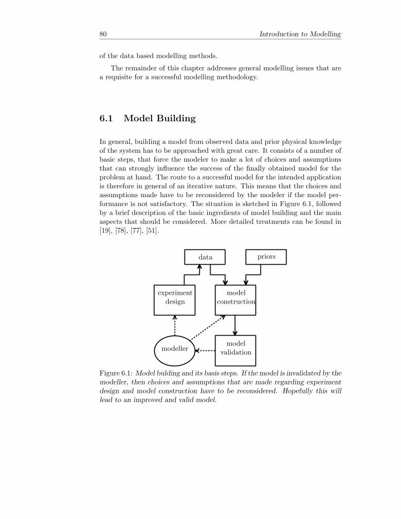
80 Introduction to Modelling
of the data based modelling methods.
The remainder of this chapter addresses general modelling issues that area requisite for a successful modelling methodology.
6.1 Model Building
In general, building a model from observed data and prior physical knowledgeof the system has to be approached with great care. It consists of a number ofbasic steps, that force the modeler to make a lot of choices and assumptionsthat can strongly influence the success of the finally obtained model for theproblem at hand. The route to a successful model for the intended applicationis therefore in general of an iterative nature. This means that the choices andassumptions made have to be reconsidered by the modeler if the model per-formance is not satisfactory. The situation is sketched in Figure 6.1, followedby a brief description of the basic ingredients of model building and the mainaspects that should be considered. More detailed treatments can be found in[19], [78], [77], [51].
data priors
experimentdesign
modelconstruction
modelvalidationmodeller
Figure 6.1: Model bulding and its basis steps. If the model is invalidated by themodeller, then choices and assumptions that are made regarding experimentdesign and model construction have to be reconsidered. Hopefully this willlead to an improved and valid model.

6.2 Experiment Design 81
6.2 Experiment Design
To design an experiment means to design an input signal for the data generat-ing system in order to extract information from the generated data, sufficientto identify1 a PLM from an a priori proposed model set, that is successfulfor the modelling task at hand. Design of a suitable input signal is not aneasy task. The shape of the input signal together with the required numberof data points have to be determined. Since nonlinear systems are considered,not only the frequency range of the input signal but also its amplitude is ofgreat importance, in order to excite the system everywhere in the operatingspace. Satisfactory results were obtained for the PLM by applying a low fre-quent signal with a large amplitude, with on top of it a small amplitude signalcontaining a broad spectrum of higher frequencies [68], [32], [72]. Similar in-put shaping strategies are reported in literature, e.g. [47]. Intuitively, it isclear that the number of data points that are needed depends on the smooth-ness of the system, and the dimensionality of the operating space. If oneviews approximation as an hypersurface reconstruction problem then becauseof limited data it is not known how regular this hypersurface is in betweenthe data points. On the other hand, many more data points are needed tofill a three dimensional cube than a two dimensional cube. This is known asthe curse of dimensionality, because complexity grows exponentially with thedimension. Furthermore, the number of data points needed depends upon thenumber of unknown parameters that have to be identified. One could say thatthe total amount of information that is present in a data sequence is bounded;when this information has to be divided over a larger set of unknown param-eters the information-per-parameter is reduced leading to a lower confidencelevel about the estimates. Of course prior knowledge can reveal some of theseproblems. One can use regime information to create more dense data sets forsome regions, thereby reflecting complexity of the underlying system. If thenumber of scheduling variables can be reduced with respect to the numberof operating variables then also the number of parameters that have to beidentified is reduced. Also, constraining the model set by restricting to locallyvalid models with predefined structure, results in less parameters that have tobe identified. This also positively affects the amount of data needed for theidentification.
1Identification means here building a representative model from the collected data of thesystem.
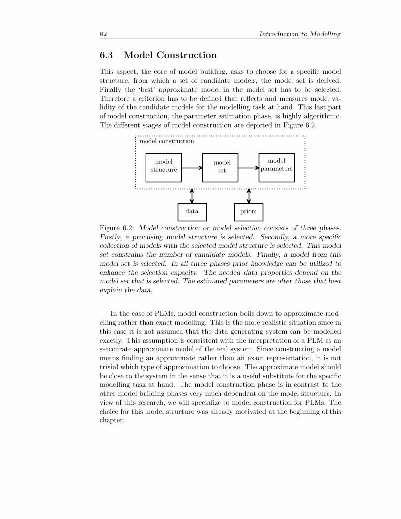
82 Introduction to Modelling
6.3 Model Construction
This aspect, the core of model building, asks to choose for a specific modelstructure, from which a set of candidate models, the model set is derived.Finally the ‘best’ approximate model in the model set has to be selected.Therefore a criterion has to be defined that reflects and measures model va-lidity of the candidate models for the modelling task at hand. This last partof model construction, the parameter estimation phase, is highly algorithmic.The different stages of model construction are depicted in Figure 6.2.
modelstructure
modelset
modelparameters
data priors
model construction
Figure 6.2: Model construction or model selection consists of three phases.Firstly, a promising model structure is selected. Secondly, a more specificcollection of models with the selected model structure is selected. This modelset constrains the number of candidate models. Finally, a model from thismodel set is selected. In all three phases prior knowledge can be utilized toenhance the selection capacity. The needed data properties depend on themodel set that is selected. The estimated parameters are often those that bestexplain the data.
In the case of PLMs, model construction boils down to approximate mod-elling rather than exact modelling. This is the more realistic situation since inthis case it is not assumed that the data generating system can be modelledexactly. This assumption is consistent with the interpretation of a PLM as anε-accurate approximate model of the real system. Since constructing a modelmeans finding an approximate rather than an exact representation, it is nottrivial which type of approximation to choose. The approximate model shouldbe close to the system in the sense that it is a useful substitute for the specificmodelling task at hand. The model construction phase is in contrast to theother model building phases very much dependent on the model structure. Inview of this research, we will specialize to model construction for PLMs. Thechoice for this model structure was already motivated at the beginning of thischapter.

6.3 Model Construction 83
Despite the fact that validity of a given model will depend on its ultimateuse, there are also application independent criteria that reflect the qualityof an approximate model. That is the trade-off between the conflicting re-quirements, a small approximation error and a small estimation error, whichis similar to the bias-variance trade-off in statistics and in system identifica-tion [58]. Firstly, if the system is assumed to be outside the representationcapacity of the selected model set then always an error between the systemand its approximation will exist, even if an infinite data set was available. Inthis context, a class of models that has large representational power is referredto as a class of high model complexity or flexibility. The error that the bestapproximate model in the model set makes is referred to as the approximationerror (bias in statistics). From the preceding chapter on approximation weknow that for PLMs it holds that the approximation error dfg is proportionalto N
−1/nm , where Nm is the number of locally valid models and n equals the di-
mension of the scheduling space. From this it follows that for high dimensionalmodelling problems n 1, the curse of dimensionality complicates model con-struction. Secondly, we do not have an infinite amount of data available butonly a finite set of data points from which we construct the model. There-fore, different data sets convey different information on the system, and themodel constructed from the finite data set might not be the best approximatemodel. This results in an additional error, the estimation error (variance instatistics). With respect to the data side of the problem, the amount andtype of data needed to ensure a small estimation error is referred to as thesample complexity. The approximation error and the estimation error are twocomponents of the generalization error. The model complexity, the samplecomplexity and the generalization error are therefore related. The relation isillustrated in Figure 6.3.
Simply, the approximation error results from a finite parameter set andthe estimation error is due to finite data (and/or noise). Simple models wouldhave high approximation errors but low estimation errors while for complexmodels the opposite would be true. Schematized this is shown in Figure 6.4.Two different sets of eight data points generated by an underlying mapping aregiven and two models different in complexity are fitted to the data. Both havea large generalization error. Whereas in Figure 6.4a this is the result of a largeestimation error, in Figure 6.4b this is the result of a large approximation error.With the more complex model the two different data sets lead to two modelsthat differ substantially; the model is sensitive to the finite data set. The modelof low complexity is much less sensitive to the finite data set; the two differentdata sets lead to two models that do not differ substantially. The trade-offbetween model complexity and sample complexity is manifest in that complexmodels can fit many functions but need large amount of data, while simple
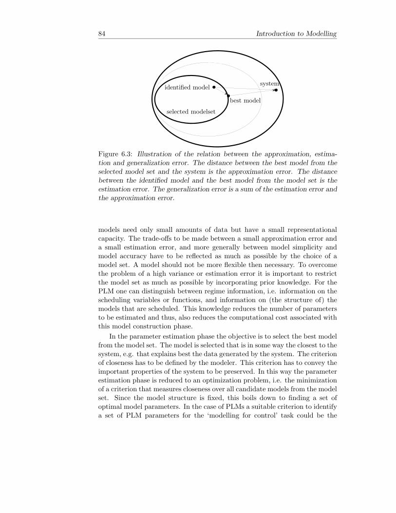
84 Introduction to Modelling
selected modelset
identified model
best model
system
Figure 6.3: Illustration of the relation between the approximation, estima-tion and generalization error. The distance between the best model from theselected model set and the system is the approximation error. The distancebetween the identified model and the best model from the model set is theestimation error. The generalization error is a sum of the estimation error andthe approximation error.
models need only small amounts of data but have a small representationalcapacity. The trade-offs to be made between a small approximation error anda small estimation error, and more generally between model simplicity andmodel accuracy have to be reflected as much as possible by the choice of amodel set. A model should not be more flexible then necessary. To overcomethe problem of a high variance or estimation error it is important to restrictthe model set as much as possible by incorporating prior knowledge. For thePLM one can distinguish between regime information, i.e. information on thescheduling variables or functions, and information on (the structure of) themodels that are scheduled. This knowledge reduces the number of parametersto be estimated and thus, also reduces the computational cost associated withthis model construction phase.
In the parameter estimation phase the objective is to select the best modelfrom the model set. The model is selected that is in some way the closest to thesystem, e.g. that explains best the data generated by the system. The criterionof closeness has to be defined by the modeler. This criterion has to convey theimportant properties of the system to be preserved. In this way the parameterestimation phase is reduced to an optimization problem, i.e. the minimizationof a criterion that measures closeness over all candidate models from the modelset. Since the model structure is fixed, this boils down to finding a set ofoptimal model parameters. In the case of PLMs a suitable criterion to identifya set of PLM parameters for the ‘modelling for control’ task could be the
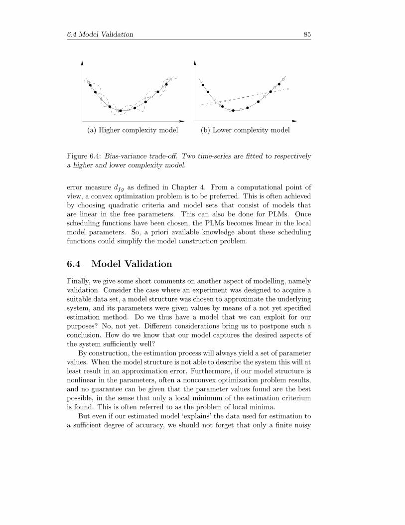
6.4 Model Validation 85
(a) Higher complexity model (b) Lower complexity model
Figure 6.4: Bias-variance trade-off. Two time-series are fitted to respectivelya higher and lower complexity model.
error measure dfg as defined in Chapter 4. From a computational point ofview, a convex optimization problem is to be preferred. This is often achievedby choosing quadratic criteria and model sets that consist of models thatare linear in the free parameters. This can also be done for PLMs. Oncescheduling functions have been chosen, the PLMs becomes linear in the localmodel parameters. So, a priori available knowledge about these schedulingfunctions could simplify the model construction problem.
6.4 Model Validation
Finally, we give some short comments on another aspect of modelling, namelyvalidation. Consider the case where an experiment was designed to acquire asuitable data set, a model structure was chosen to approximate the underlyingsystem, and its parameters were given values by means of a not yet specifiedestimation method. Do we thus have a model that we can exploit for ourpurposes? No, not yet. Different considerations bring us to postpone such aconclusion. How do we know that our model captures the desired aspects ofthe system sufficiently well?
By construction, the estimation process will always yield a set of parametervalues. When the model structure is not able to describe the system this will atleast result in an approximation error. Furthermore, if our model structure isnonlinear in the parameters, often a nonconvex optimization problem results,and no guarantee can be given that the parameter values found are the bestpossible, in the sense that only a local minimum of the estimation criteriumis found. This is often referred to as the problem of local minima.
But even if our estimated model ‘explains’ the data used for estimation toa sufficient degree of accuracy, we should not forget that only a finite noisy

86 Introduction to Modelling
data set was used. It is quite possible that when confronted with a ‘fresh’ dataset from the system, the model will perform not as well due to the estimationerror, which, is the result of a model structure of high complexity combinedwith a small data set. On the other hand, it is also possible that the dataset used for estimation of the model parameter values did not cover all thesystem’s peculiarities or regions to a sufficient degree; this is a problem ofpersistence of excitation.
The last problem can be solved by arranging an experiment which givesus a data set that does fulfill the condition of persistence of excitation. Butas already mentioned, in general this is not an easy task.
To reduce the probability of not reaching the minimal possible value ofthe estimation criterium, the estimation of the parameter values is repeatedseveral times for the same model structure under slightly varying (starting)conditions. This gives us some assurance that the ‘best’ model within a par-ticular model structure, given a particular data set, has been found. However,it is not clear if this is what we want, since this ‘best’ model that minimizesthe estimation criterium is based on a particular finite data set, and a largeestimation error may be the result. We actually want a small generalizationerror. It is possible that the ‘best’ model as the term is used in this paragraphhas a larger generalization error than a slightly ‘worse’ model.
Several validation methods have been devised which all try to alarm us incase we come across some of the mentioned pitfalls. The most obvious andpragmatic way of validation is to investigate how well the model is capableof reproducing the system behavior on a new set of data (the cross-validationdata) that was not used to fit the model. That is, we supply both the modeland the system with an input different from the one used to obtain the esti-mation data set, and compare the model and system output afterwards. Wemay visually inspect the result or use a more quantitative measure of fit, e.g.,the root-mean-square value of the difference between the outputs.
A second basic method for model validation is to examine the residu-als (‘leftovers’) from the estimation process, i.e. the differences between themeasured and the estimated output. The advantage hereby is that separatevalidation data sets are not necessary. A number of statistical residual anal-ysis tests can be performed to see if what the model could not ‘explain’ stillcontains traces of a deterministic nature, e.g., unmodelled dynamics. For adetailed treatment the reader is referred to [21], [50], [15]. These tests can alsobe applied to a validation data set.
If possible, it is wise to use all the available a priori information to validatethe model, for instance, does the model make physically sense? Since thePLM has locally a clear physical interpretation, its parameter values can bequalitatively validated by inspection.
Besides these application independent criteria for assessing the quality of

6.4 Model Validation 87
a model, validity of a proposed model should in the first place be judged byits success within the intended model application.

88 Introduction to Modelling
Chapter 7
Building PLMs from knownNonlinear Models
7.1 Introduction
In this chapter a model based modelling method is considered. It is assumedthat a nonlinear model of the system is available. The method is based uponthe approximation results that were derived in Chapter 4. It automaticallydecomposes the operating space in qualitatively different operating regimes,and subsequently specifies a scheduling function and a linear model for eachregime. For notational convenience the modelling method is presented forsystems without an output equation, i.e. (7.1), nonetheless (by augmenting theright-hand side of the system with the right-hand side of the output equation)it naturally extends to systems with outputs [81].
A novel method is developed that, given an a priori sufficiently smoothnonlinear continuous time state space description of the system
x = f(x, u) (7.1)
with the state x ∈ X ⊆ Rn, the manipulated input u ∈ U ⊆ R
m, automaticallyconstructs a PLM
x =Nm∑i=1
wi(x, u)Aix + Biu + ai (7.2)
= g(x, u)
with Nm as small as possible, and such that within the region of interest, acompact operating space Ψ ⊆ X × U ,
dfg(Ψ) ≤ ε (7.3)
89

90 Building PLMs from known Nonlinear Models
with ε > 0 pre-specified by the modeler.The distance dfg between the right-hand side of the system and the PLM
was already defined in (4.1). It is known from Theorem 4.6.3 that with thisparticular choice of distance between the system and the PLM, an upper boundfor the number of scheduling regimes Nm can be computed, sufficient to ensurethe existence of an ε-accurate PLM. A PLM that achieves this accuracy isbuilt from a set of Nm Taylor series expansions of the system, equidistantlydistributed over the scheduling space Z.
The above-mentioned upper bound, will be denoted by Nupperm and is based
on a worst-case situation. It is assumed that the maximum nonlinearity asmeasured with an upper bound on the Taylor remainders corresponding tothe aforementioned Taylor series expansions, is attained everywhere in thescheduling space, and as a consequence the scheduling space is uniformly par-titioned into scheduling regimes.
Thus the objective is to select an ε-accurate PLM from the model set
M(Nm ≤ Nupperm ) := (7.2) | Nm ≤ Nupper
m (7.4)
with Nm as small as possible. Determination of a PLM∈ M(Nm ≤ Nupperm )
implies that a PLM from the model set has to be selection. The modellingproblem can be divided into three subproblems that are solved sequentially.
problem 1: operating space → scheduling space The scheduling spaceis determined. The dimension of the scheduling space is reduced as muchas possible compared to the operating space, since Nm grows exponen-tially with the dimension of the scheduling space Z.
problem 2: scheduling space → scheduling regimes The Nm schedul-ing regimes Zi are determined. The number of scheduling regimes Nm
is reduced as much as possible. The result is a nonuniform partitioningof the scheduling space.
problem 3: scheduling regimes → PLM parameters The parametersare determined either by linearization of the system in the centers ofthe obtained operating regimes or by a least squares fitting procedure.
In each of the three steps the model set is restricted and the number ofcandidate PLMs is eventually reduced to one. In Section 7.2 through Section7.4 a more in depth description of the three subproblems is given as well asa solution to each of the three subproblems is suggested. The situation isdepicted in Figure 7.1.
In Section 7.5 the modelling method is illustrated by two examples, themodelling of two nonlinear mechanical systems. Finally, in Section 7.6, somenotes and comments are made regarding the proposed method.
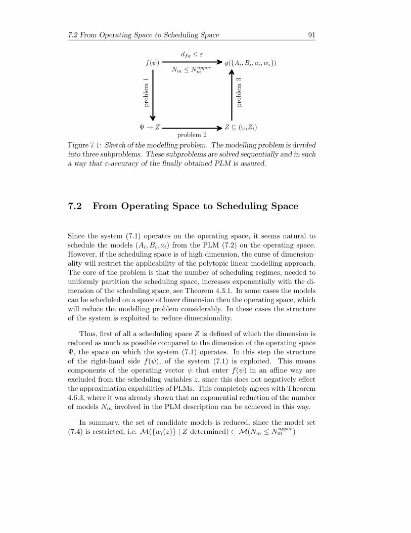
7.2 From Operating Space to Scheduling Space 91
f(ψ)
Ψ→ Z Z ⊆ (∪iZi)
g(Ai, Bi, ai, wi)
prob
lem
1
problem 2
prob
lem
3
dfg ≤ ε
Nm ≤ Nupperm
Figure 7.1: Sketch of the modelling problem. The modelling problem is dividedinto three subproblems. These subproblems are solved sequentially and in sucha way that ε-accuracy of the finally obtained PLM is assured.
7.2 From Operating Space to Scheduling Space
Since the system (7.1) operates on the operating space, it seems natural toschedule the models (Ai, Bi, ai) from the PLM (7.2) on the operating space.However, if the scheduling space is of high dimension, the curse of dimension-ality will restrict the applicability of the polytopic linear modelling approach.The core of the problem is that the number of scheduling regimes, needed touniformly partition the scheduling space, increases exponentially with the di-mension of the scheduling space, see Theorem 4.3.1. In some cases the modelscan be scheduled on a space of lower dimension then the operating space, whichwill reduce the modelling problem considerably. In these cases the structureof the system is exploited to reduce dimensionality.
Thus, first of all a scheduling space Z is defined of which the dimension isreduced as much as possible compared to the dimension of the operating spaceΨ, the space on which the system (7.1) operates. In this step the structureof the right-hand side f(ψ), of the system (7.1) is exploited. This meanscomponents of the operating vector ψ that enter f(ψ) in an affine way areexcluded from the scheduling variables z, since this does not negatively effectthe approximation capabilities of PLMs. This completely agrees with Theorem4.6.3, where it was already shown that an exponential reduction of the numberof models Nm involved in the PLM description can be achieved in this way.
In summary, the set of candidate models is reduced, since the model set(7.4) is restricted, i.e. M(wi(z) | Z determined) ⊂M(Nm ≤ Nupper
m )
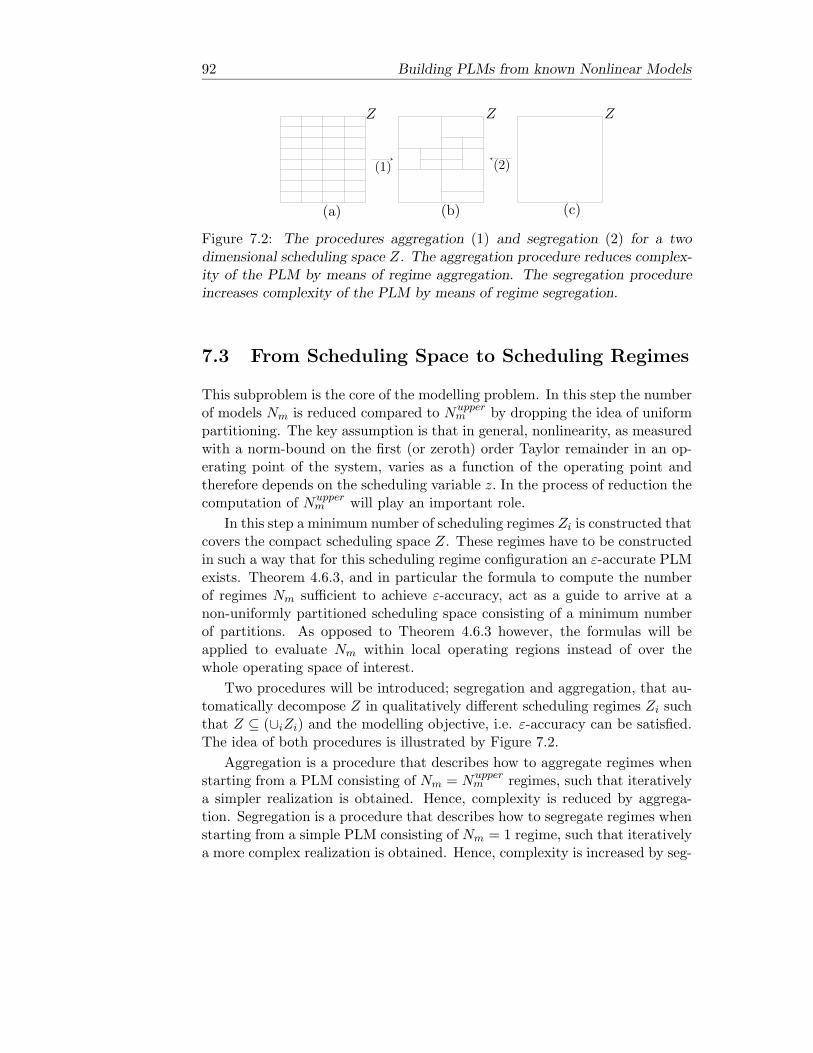
92 Building PLMs from known Nonlinear Models
ZZZ
(1) (2)
(a) (b) (c)
Figure 7.2: The procedures aggregation (1) and segregation (2) for a twodimensional scheduling space Z. The aggregation procedure reduces complex-ity of the PLM by means of regime aggregation. The segregation procedureincreases complexity of the PLM by means of regime segregation.
7.3 From Scheduling Space to Scheduling Regimes
This subproblem is the core of the modelling problem. In this step the numberof models Nm is reduced compared to Nupper
m by dropping the idea of uniformpartitioning. The key assumption is that in general, nonlinearity, as measuredwith a norm-bound on the first (or zeroth) order Taylor remainder in an op-erating point of the system, varies as a function of the operating point andtherefore depends on the scheduling variable z. In the process of reduction thecomputation of Nupper
m will play an important role.In this step a minimum number of scheduling regimes Zi is constructed that
covers the compact scheduling space Z. These regimes have to be constructedin such a way that for this scheduling regime configuration an ε-accurate PLMexists. Theorem 4.6.3, and in particular the formula to compute the numberof regimes Nm sufficient to achieve ε-accuracy, act as a guide to arrive at anon-uniformly partitioned scheduling space consisting of a minimum numberof partitions. As opposed to Theorem 4.6.3 however, the formulas will beapplied to evaluate Nm within local operating regions instead of over thewhole operating space of interest.
Two procedures will be introduced; segregation and aggregation, that au-tomatically decompose Z in qualitatively different scheduling regimes Zi suchthat Z ⊆ (∪iZi) and the modelling objective, i.e. ε-accuracy can be satisfied.The idea of both procedures is illustrated by Figure 7.2.
Aggregation is a procedure that describes how to aggregate regimes whenstarting from a PLM consisting of Nm = Nupper
m regimes, such that iterativelya simpler realization is obtained. Hence, complexity is reduced by aggrega-tion. Segregation is a procedure that describes how to segregate regimes whenstarting from a simple PLM consisting of Nm = 1 regime, such that iterativelya more complex realization is obtained. Hence, complexity is increased by seg-
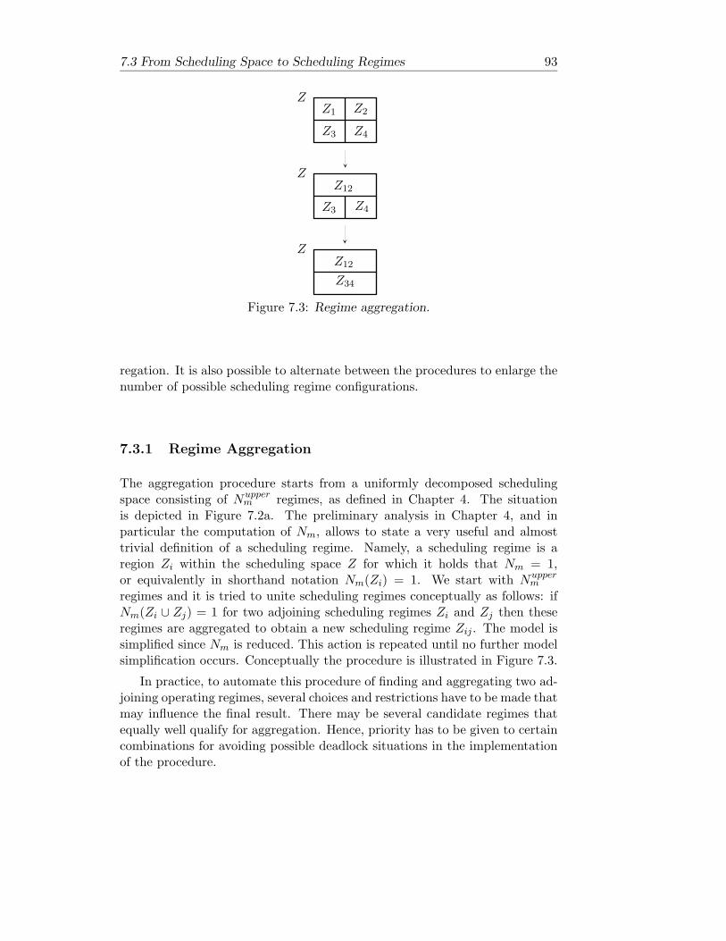
7.3 From Scheduling Space to Scheduling Regimes 93
Z
Z
Z
Z1 Z2
Z3
Z3
Z4
Z4
Z12
Z12
Z34
Figure 7.3: Regime aggregation.
regation. It is also possible to alternate between the procedures to enlarge thenumber of possible scheduling regime configurations.
7.3.1 Regime Aggregation
The aggregation procedure starts from a uniformly decomposed schedulingspace consisting of Nupper
m regimes, as defined in Chapter 4. The situationis depicted in Figure 7.2a. The preliminary analysis in Chapter 4, and inparticular the computation of Nm, allows to state a very useful and almosttrivial definition of a scheduling regime. Namely, a scheduling regime is aregion Zi within the scheduling space Z for which it holds that Nm = 1,or equivalently in shorthand notation Nm(Zi) = 1. We start with Nupper
m
regimes and it is tried to unite scheduling regimes conceptually as follows: ifNm(Zi ∪ Zj) = 1 for two adjoining scheduling regimes Zi and Zj then theseregimes are aggregated to obtain a new scheduling regime Zij . The model issimplified since Nm is reduced. This action is repeated until no further modelsimplification occurs. Conceptually the procedure is illustrated in Figure 7.3.
In practice, to automate this procedure of finding and aggregating two ad-joining operating regimes, several choices and restrictions have to be made thatmay influence the final result. There may be several candidate regimes thatequally well qualify for aggregation. Hence, priority has to be given to certaincombinations for avoiding possible deadlock situations in the implementationof the procedure.
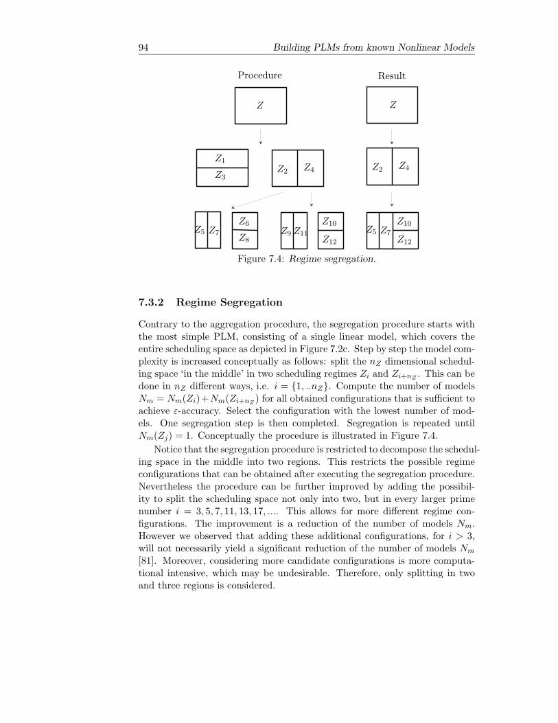
94 Building PLMs from known Nonlinear Models
ZZ
Z1Z2Z2Z3
Z4Z4
Z5Z5
Z6Z7Z7
Z8Z9
Z10Z10Z11
Z12Z12
Procedure Result
Figure 7.4: Regime segregation.
7.3.2 Regime Segregation
Contrary to the aggregation procedure, the segregation procedure starts withthe most simple PLM, consisting of a single linear model, which covers theentire scheduling space as depicted in Figure 7.2c. Step by step the model com-plexity is increased conceptually as follows: split the nZ dimensional schedul-ing space ‘in the middle’ in two scheduling regimes Zi and Zi+nZ . This can bedone in nZ different ways, i.e. i = 1, ..nZ. Compute the number of modelsNm = Nm(Zi)+Nm(Zi+nZ ) for all obtained configurations that is sufficient toachieve ε-accuracy. Select the configuration with the lowest number of mod-els. One segregation step is then completed. Segregation is repeated untilNm(Zj) = 1. Conceptually the procedure is illustrated in Figure 7.4.
Notice that the segregation procedure is restricted to decompose the schedul-ing space in the middle into two regions. This restricts the possible regimeconfigurations that can be obtained after executing the segregation procedure.Nevertheless the procedure can be further improved by adding the possibil-ity to split the scheduling space not only into two, but in every larger primenumber i = 3, 5, 7, 11, 13, 17, .... This allows for more different regime con-figurations. The improvement is a reduction of the number of models Nm.However we observed that adding these additional configurations, for i > 3,will not necessarily yield a significant reduction of the number of models Nm
[81]. Moreover, considering more candidate configurations is more computa-tional intensive, which may be undesirable. Therefore, only splitting in twoand three regions is considered.

7.4 From Scheduling Regimes to PLM Parameters 95
7.4 From Scheduling Regimes to PLM Parameters
Two procedures were presented, aggregation and segregation, that decomposethe scheduling space Z in Nm disjoint regions Zi, such that ε-accuracy canbe achieved. A scheduling regime Zi is characterized by its center z0i andwidth ri. For each scheduling regime Zi a model Mi, the triple (Ai, Bi, ai) willbe defined together with a scheduling function wi(θi), ergo the PLM will bespecified. If the scheduling function parameters θi are to be computed simul-taneously with the model parameters Mi a complex nonlinear programmingproblem results. We like to point out that our experience obtained with theprocedures aggregation and segregation, indicates that the qualitative infor-mation, concerning the validity of the scheduling regimes, provides enoughknowledge to construct the scheduling functions.
The scheduling functions are chosen as normalized basis functions, centeredin the middle of operating regime i and with support in accordance with thesize of scheduling regime Zi. The parameters of the linear models are eitherobtained by linearization of the system in the centers of the scheduling space,or by a least squares fitting procedure.
7.4.1 Constructing Scheduling Functions
The scheduling functions are the result of a normalization of a set of basisfunctions, the model validity functions ρi. For instance as in (3.6)
wi(z, θi) =ρi(z, θi)∑Nmj=1 ρj(z, θi)
A few possible choices for the ρi functions are given in Example 4.2.3. Thebasis functions ρi have support in the region Zi and tend to zero outside thisregion. Furthermore
∑Nmi=1 ρi(z) ≥ 0 for all z ∈ Z. A common choice is the
multivariate Gaussian function (4.8):
ρi(z, θi) = e−(z−θi1)TΘ−1
i (z−θi1)
where Θi = 2diag(σij) with j = 1, ...,dim(z), and θi = [θi1,Θi] are the un-knowns to be determined. The unknowns denoted by θi are expressed as afunction of the centre z0i and width ri of regime Zi. Typically the maximumvalue of ρi(z) is attained in z0i, which is ‘the centre’ of operating regime Zi,that was determined with the procedure aggregation or segregation. Thereforeθi1 = z0i. The variance matrix Θi is expressed as a function of the width riof the scheduling regime, i.e. Θi = γIri. Here γ is a scaling parameter thatconsiders the overlap between the validity functions. A typical value of γ isbetween 0.25 and 2. There will almost be no overlap when γ = 0.25 and a

96 Building PLMs from known Nonlinear Models
large overlap when γ = 2. Sometimes prior knowledge about the system isa good guide for the choice of γ. It may appear that the choice of the typeof validity function has significant impact on the model. However it is ourexperience that both the efficacy of the algorithm and the model predictionsare quite insensitive with respect to this choice, hence the specification of thetype of validity function does not seem to require much prior knowledge ofthe system. On the other hand, the choice of the user specified parameter γappears to be of major influence.
7.4.2 Constructing Linear Model Parameters by Linearizations
It is known from Chapter 4 that with the adopted choice of distance betweensystems, an ε-accurate PLM is ensured if the model parameters are chosen aslinearizations of the system around ψ0i, the centers of the operating regimes.This statement still being valid, a useful choice for the model parameters is:
Ai = ∂f∂x (ψ0i) Bi = ∂f
∂u(ψ0i) ai = f(ψ0i)− ∂f∂ψ (ψ0i)ψ0i (7.5)
7.4.3 Constructing Linear Model Parameters by Least Squares
Another method which yields good results, is to determine the model param-eters with a least squares method. Therefore the system is linearized in Ng
points ψ0i, uniformly scattered over the scheduling space. Evidently it is notpossible to linearize the system in every point of the operating space. It isimportant that Ng Nm, to assure enough information is available to com-pute reliable model parameters. At the points of linearization, i.e. ψ0i withi = 1, ..., Ng the obtained linearized model is an exact representation of thesystem and becomes
x = A(ψ0i)x + B(ψ0i)u + a(ψ0i)
Here the matrices are defined as in (7.5). For the Ng points we can write forthe error between the system and the PLM
A(ψ0i)x + B(ψ0i)u + a(ψ0i)−Nm∑j=1
wj(ψ0i)Aix + Biu + ai = EABa,i
where i = 1, ..., Ng. This error can be split in different parts to reflect thecontribution of the different components of the PLM description, i.e. EABa,i =EA,i + EB,i + Ea,i with
EA,i = A(ψ0i)−Nm∑j=1
wj(ψ0i)Aj

7.4 From Scheduling Regimes to PLM Parameters 97
Similar expressions hold for the matrices EB,i and Ea,i. Note that the numberNm and the scheduling functions wj are already determined as a result of theapplication of the aggregation or segregation procedure.
For the first part of EABa,i, i.e. EA,i, the objective is to minimize the costfunction
J(Aj) =Ng∑i=1
‖EA,i‖2F (7.6)
with respect to the unknown parameters Aj with j = 1, ..., Nm. Here
‖E‖F =√√√√ ∑
1≤i≤n1≤j≤m
|E(i, j)|2
is the Frobenius norm of the matrix E ∈ Rn∗m, i.e. the square root of the
sums of the squares of the entries of the matrix E. Similar expressions holdfor J(Bj) and J(aj). In the sequel the least squares estimates for Ajare derived. The remaining unknown parameters Bj , aj can be obtainedsimilarly. Thus
‖EA,i‖2F =n∑
j,k=1
|EA,i(j, k)|2
=n∑
j,k=1
∣∣∣∣∣A(ψ0i)(j, k)−Nm∑l=1
wl(ψ0i)Al(j, k)
∣∣∣∣∣2
=n∑
j,k=1
∣∣A(ψ0i)(j, k)− w(ψ0i)TAPLM (j, k)∣∣2
where
w(ψ0i)T = [w1(ψ0i), · · · , wNm(ψ0i)]
and
APLM (j, k) = [A1(j, k), · · · , ANm(j, k)]T .
With
W T = [w(ψ01), · · · , w(ψ0Ng)]
and
A(j, k) = [A(ψ01)(j, k), · · · , A(ψ0Ng)(j, k)]T

98 Building PLMs from known Nonlinear Models
the cost function (7.6) becomes
J(Ai) =n∑
j,k=1
‖A(j, k)−WAPLM (j, k)‖2
The least square estimate is
APLM (j, k) = (W TW )−1W TA(j, k)
The other free parameters of the PLM can be determined in the same way,i.e.,
BPLM (j, l) = (W TW )−1W TB(j, l)
and
aPLM (j) = (W TW )−1W Ta(j)
7.5 Examples
The modelling method, as it was described in this section will be illustratedby two examples. In each of the two examples the objective is to derive thesimplest ε accurate PLM. It is assumed that a suitable white-box model for thesystem is available. The two systems under consideration belong to the classof nonlinear mechanical systems that are often encountered in applications[57]. The state space equations describing systems of this particular class are
d
dt
]=[
q−M(q)−1(C(q, q) + k(q))
]+[
0M(q)−1B
]u (7.7)
with input u and state x = [q, q]T , where q are the displacements and q thevelocities. Here M(q) is the positive definite mass matrix, B is denoted thedistribution matrix, k(q) represents the conservative generalized forces, andC(q, q) comprehends the remaining generalized forces such as the Coriolis,centrifugal and friction components. The particular structure of the model(7.7) will be exploited in the two examples. More specifically, since the inputenters the system in an affine way, this variable can be excluded from theset of scheduling variables without affecting the approximation capability ofthe PLM, thereby reducing the complexity of the modelling problem. In thisway the set of candidate PLMs is reduced. This is in fact the result of theapplication of Theorem 4.6.3, and as already mentioned, a possible solution tothe first of the three subproblems in which the modelling problem was divided(see Figure 7.1).

7.5 Examples 99
The first example, i.e. modelling of a rotating robot arm subjected to sig-nificant friction in the drive line, shows a local nonlinearity. This implies thaton any non-compact operating region an ε-accurate PLM exists, consisting ofa finite number of models, in contrast to a system that features a global non-linearity. Because of the strongly local character of the nonlinearity, i.e. thefriction torque characteristic, we expect that the number of models Nm will bereduced significantly as compared to Nupper
m , see Theorem 4.6.3, by droppingthe idea of uniform partitioning and applying the aggregation or segregationprocedure.
The second example, i.e. modelling of an inverted pendulum on a cart,shows a global nonlinearity. This system is more complex in the sense thatthe scheduling space is two dimensional instead of one dimensional. Because ofthe global nonlinearity, the reduction of Nm is expected to be less significant,as compared to the previous example.
The examples will illustrate the modelling method and its features. Thechoice for the two white-box models used in the examples is motivated bythe fact that they show great similarity with those located in our laboratory.The modelling method was automated as a Matlab implementation. A moredetailed description of the modelling method for these specific examples canbe found in [81] and [11].
7.5.1 A Rotational Robotic Manipulator System
Consider the rotating robot arm from Figure 7.5, which is subjected to signifi-cant friction in the driveline. The rotating robot arm is a nonlinear mechanical
q
u
Figure 7.5: Rotational robotic manipulator.
system with one degree of freedom q, where q represents the angular displace-ment of the arm, and u is the motor input current. The state space equations(7.7) reduce to
d
dt
]=[
q−M−1C(q)
]+[
0M−1B
]u (7.8)

100 Building PLMs from known Nonlinear Models
with M = 0.0292 [Nms2] the effective inertia of the motor-transmission-rotating arm combination, B = 16 [NmV −1] is the motor gain, and C(q) isthe friction torque. Friction models that are often used for modelling purposesare depicted in Figure 7.6. A survey on friction models is given in [32]. The
velocityvelocity
velocityvelocity
friction torque
friction torquefriction torque
friction torque
(b)(a)
(c) (d)
Figure 7.6: Friction models. (a) viscous friction model, (b) Coulomb+viscousfriction model, (c) Coulomb+viscous+Stribeck friction model, (d) continuousCoulomb+viscous+Stribeck friction model.
friction torque is assumed to be a continuous friction model consisting of aCoulomb part (Cc), a viscous friction part (Cv), and the Stribeck frictioneffect Cs, i.e.
C(q) = Cc(q) + Cv(q) + Cs(q)
where
Cc(q) = Tc2π
arctan(κq)
Cs(q) = (Ts − Tc)e−(qvs
)2 2π
arctan(κq)
Cv(q) = σq
See Figure 7.6d for the qualitative relation between friction torque and angularvelocity. The friction parameters values are Tc = 0.416 [Nm], Ts = 0.4657[Nm], vs = 0.2 [rad/s], σ = 0.0135 [Nms], κ = 1000[−]. All the parametervalues are estimates obtained from measurements on a real rotating robotarm in the mechanical engineering laboratory. The unknown parameters wereestimated with standard parameter estimation methods [22].
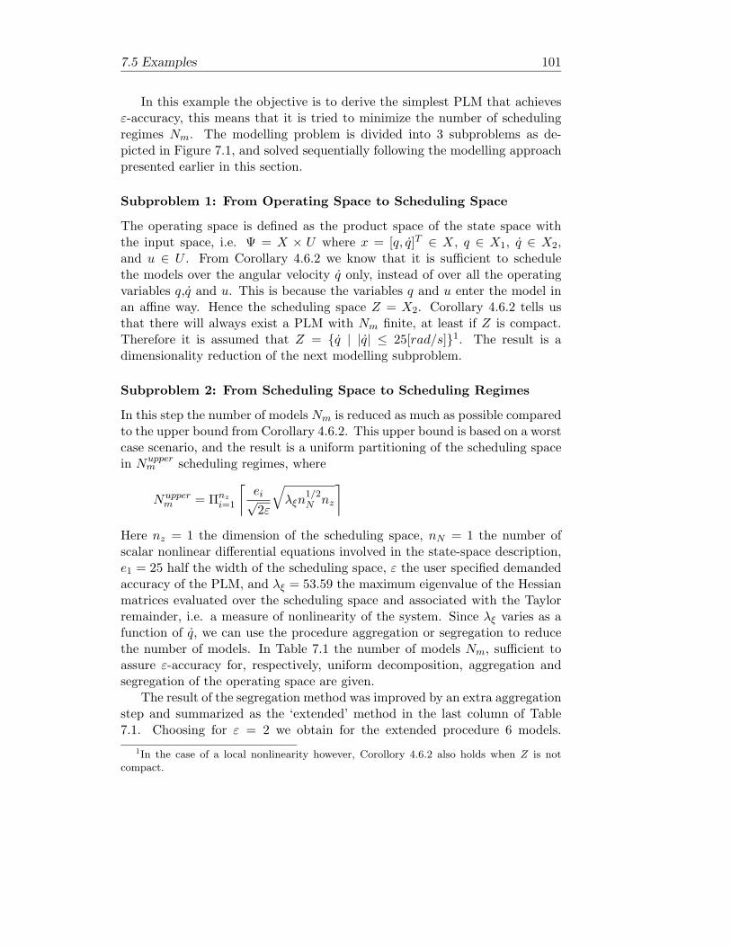
7.5 Examples 101
In this example the objective is to derive the simplest PLM that achievesε-accuracy, this means that it is tried to minimize the number of schedulingregimes Nm. The modelling problem is divided into 3 subproblems as de-picted in Figure 7.1, and solved sequentially following the modelling approachpresented earlier in this section.
Subproblem 1: From Operating Space to Scheduling Space
The operating space is defined as the product space of the state space withthe input space, i.e. Ψ = X × U where x = [q, q]T ∈ X, q ∈ X1, q ∈ X2,and u ∈ U . From Corollary 4.6.2 we know that it is sufficient to schedulethe models over the angular velocity q only, instead of over all the operatingvariables q,q and u. This is because the variables q and u enter the model inan affine way. Hence the scheduling space Z = X2. Corollary 4.6.2 tells usthat there will always exist a PLM with Nm finite, at least if Z is compact.Therefore it is assumed that Z = q | |q| ≤ 25[rad/s]1. The result is adimensionality reduction of the next modelling subproblem.
Subproblem 2: From Scheduling Space to Scheduling Regimes
In this step the number of models Nm is reduced as much as possible comparedto the upper bound from Corollary 4.6.2. This upper bound is based on a worstcase scenario, and the result is a uniform partitioning of the scheduling spacein Nupper
m scheduling regimes, where
Nupperm = Πnz
i=1
⌈ei√2ε
√λξn
1/2N nz
⌉
Here nz = 1 the dimension of the scheduling space, nN = 1 the number ofscalar nonlinear differential equations involved in the state-space description,e1 = 25 half the width of the scheduling space, ε the user specified demandedaccuracy of the PLM, and λξ = 53.59 the maximum eigenvalue of the Hessianmatrices evaluated over the scheduling space and associated with the Taylorremainder, i.e. a measure of nonlinearity of the system. Since λξ varies as afunction of q, we can use the procedure aggregation or segregation to reducethe number of models. In Table 7.1 the number of models Nm, sufficient toassure ε-accuracy for, respectively, uniform decomposition, aggregation andsegregation of the operating space are given.
The result of the segregation method was improved by an extra aggregationstep and summarized as the ‘extended’ method in the last column of Table7.1. Choosing for ε = 2 we obtain for the extended procedure 6 models.
1In the case of a local nonlinearity however, Corollory 4.6.2 also holds when Z is notcompact.
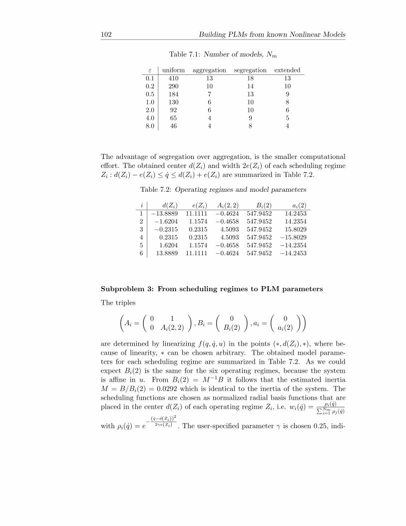
102 Building PLMs from known Nonlinear Models
Table 7.1: Number of models, Nm
ε uniform aggregation segregation extended0.1 410 13 18 130.2 290 10 14 100.5 184 7 13 91.0 130 6 10 82.0 92 6 10 64.0 65 4 9 58.0 46 4 8 4
The advantage of segregation over aggregation, is the smaller computationaleffort. The obtained center d(Zi) and width 2e(Zi) of each scheduling regimeZi : d(Zi)− e(Zi) ≤ q ≤ d(Zi) + e(Zi) are summarized in Table 7.2.
Table 7.2: Operating regimes and model parameters
i d(Zi) e(Zi) Ai(2, 2) Bi(2) ai(2)1 −13.8889 11.1111 −0.4624 547.9452 14.24532 −1.6204 1.1574 −0.4658 547.9452 14.23543 −0.2315 0.2315 4.5093 547.9452 15.80294 0.2315 0.2315 4.5093 547.9452 −15.80295 1.6204 1.1574 −0.4658 547.9452 −14.23546 13.8889 11.1111 −0.4624 547.9452 −14.2453
Subproblem 3: From scheduling regimes to PLM parameters
The triples(Ai =
(0 10 Ai(2, 2)
), Bi =
(0
Bi(2)
), ai =
(0
ai(2)
))
are determined by linearizing f(q, q, u) in the points (∗, d(Zi), ∗), where be-cause of linearity, ∗ can be chosen arbitrary. The obtained model parame-ters for each scheduling regime are summarized in Table 7.2. As we couldexpect Bi(2) is the same for the six operating regimes, because the systemis affine in u. From Bi(2) = M−1B it follows that the estimated inertiaM = B/Bi(2) = 0.0292 which is identical to the inertia of the system. Thescheduling functions are chosen as normalized radial basis functions that areplaced in the center d(Zi) of each operating regime Zi, i.e. wi(q) = ρi(q)∑Nm
i=1 ρj(q)
with ρi(q) = e− (q−d(Zi))2
2γe(Zi) . The user-specified parameter γ is chosen 0.25, indi-

7.5 Examples 103
cating almost no overlap between the models. The scheduling functions areshown in Figure 7.7.
−25 −20 −15 −10 −5 0 5 10 15 20 250
0.5
1
−25 −20 −15 −10 −5 0 5 10 15 20 250
0.5
1
−25 −20 −15 −10 −5 0 5 10 15 20 250
0.5
1
x2[rad/s]
x2[rad/s]
x2[rad/s]
w2
w1
w3
Scheduling functions
Figure 7.7: The scheduling functions w1, w2 and w3. The remaining schedul-ing functions are omitted since they follow from the symmetry around zerovelocity.
Model Validation
The friction torque of the PLM is validated and depicted together with thefriction torque of the real system in Figure 7.8. A visually identical frictioncurve compared to the system is observed. In this case
dfg = M−1 ∗maxq∈X2
‖C(q)− CPLM (q)‖2= 1/0.0292 ∗ 0.0165= 0, 5638
and thus the demanded accuracy dfg ≤ 2 is achieved.The PLM can be unraveled as follows. Regime Z1, Z2 and Z5, Z6 indicate
the viscous friction, while the regimes for low velocities, i.e. regimes Z3 and Z4
introduce a Coulomb friction and Stribeck friction component. The symmetryof the friction torque follows from the PLM parameters in Table 7.2. Theregimes are centered symmetric around zero velocity, and these symmetricregimes share the same absolute model parameter values. The symmetry ofthe system is revealed by the modelling method.

104 Building PLMs from known Nonlinear Models
−25 −20 −15 −10 −5 0 5 10 15 20 25−1
−0.5
0
0.5
1
−25 −20 −15 −10 −5 0 5 10 15 20 250
0.005
0.01
0.015
0.02
x2[rad/s]
x2[rad/s]
C(q
)andC
PL
M(q
)‖C
(q)−C
PL
M(q
)‖2
Figure 7.8: Validation of the modelled friction torque.
7.5.2 An Inverted Pendulum on a Cart
In this example the inverted pendulum as depicted in Figure 7.9 is consideredas a subject for modelling. This is a benchmark example in the literature,confer [82], [44], [85]. The inverted pendulum is again a nonlinear mechanical
q
m
M
2l
u
Figure 7.9: Inverted pendulum on a cart.
system with one degree of freedom q, where q denotes the angular displacementof the arm from the vertical axis, and u is the motor input. The state spaceequations (7.7) reduce to
d
dt
]=
[q
g sin(q)−0.5amlq2 sin(2q)4l/3−aml cos2(q)
]+
[0
−a cos(q)4l/3−aml cos2(q)
]u (7.9)

7.5 Examples 105
and are taken from [13]. Here g = 9.8m/s2 is the gravity constant, m = 2.0kgis the mass of the pendulum, M = 8.0kg is the mass of the cart, 2l = 1.0m isthe length of the pendulum, and a = 1/(m + M).
Once again the objective is to derive the simplest PLM that achieves ε-accuracy, that is the PLM that minimizes the number of scheduling regimesNm. The modelling problem is divided into 3 subproblems as depicted inFigure 7.1, and solved sequentially following the modelling approach presentedearlier in this section.
Subproblem 1: From Operating Space to Scheduling Space
The operating space is defined as the product space of the state space withthe input space, i.e. Ψ = X × U where x = [q, q]T ∈ X, q ∈ X1, q ∈ X2,and u ∈ U . From Theorem 4.6.3 we know that it is sufficient to schedule themodels over the angle q and angular velocity q, instead of over all the operatingvariables q,q and u, because the variable u enters the model in an affine way.Hence the scheduling space Z = X. Theorem 4.6.3 tells us that there willalways exist a PLM with Nm finite that achieves ε-accuracy, at least if Z iscompact, and Theorem 4.6.3 gives an upper bound for Nm. It is assumed thatZ = q, q | |q| ≤ π
2 [rad], |q| ≤ 6.5[rad/s] covers the working range of theinverted pendulum.
Subproblem 2: From Scheduling Space to Scheduling Regimes
In this step the number of models Nm is reduced as much as possible comparedto the upper bound from Theorem 4.6.3. This upper bound is based on a worstcase scenario, and the result is a uniform partitioning of the scheduling space.Since the nonlinearity varies as a function of z ∈ Z, we can use the procedureaggregation or segregation to reduce the number of models. In Table 7.3 thenumber of models Nm, sufficient to assure ε-accuracy for, respectively, uniformdecomposition, aggregation and segregation of the operating space are given.
Table 7.3: Number of models, Nm
ε uniform aggregation segregation extended0.5 324 306 281 2751.0 150 144 137 1372.0 90 88 85 854.0 39 39 43 418.0 27 27 21 2116.0 14 14 15 1332.0 10 8 11 9

106 Building PLMs from known Nonlinear Models
The result of the segregation method was improved by an extra aggregationstep and summarized as the ‘extended’ method in the last column of Table7.3. It can be noticed that, because of the global geometric nonlinearities inthe system, the upper bound is much less conservative than in the previousexample with the local nonlinearity. Choosing ε = 8, we obtain for the segre-gation method 21 models. It is difficult to determine a suitable value of ε inadvance. Typically, one starts with a value, validates the result, and increasesor decreases the value if one is not satisfied with the validation result.
The centres d(Zi) and the widths 2e(Zi) of each operating regime Zi :
d(Zi) − e(Zi) ≤ (z =[
]) ≤ d(Zi) + e(Zi), where d(Zi) =
[d1(Zi)d2(Zi)
]and
e(Zi) =[
e1(Zi)e2(Zi)
]are summarized in Table 7.4.
Table 7.4: Operating regimes and model parameters
i d1(Zi) d2(Zi) e1(Zi) e2(Zi) Ai(2, 1) Ai(2, 2) Bi(2) ai(2)1 -1.0472 -1.4444 0.5236 0.7222 6.0328 -0.1949 -0.0779 -7.04982 -1.0472 0 0.5236 0.7222 5.8512 0 -0.0779 -7.09923 -1.0472 1.4444 0.5236 0.7222 6.0328 0.1949 -0.0779 -7.04984 -0.7854 2.8889 0.7854 0.7222 9.5247 0.4685 -0.1147 -4.43325 -0.7854 4.3333 0.7854 0.7222 9.6619 0.7027 -0.1147 -5.17136 -0.7854 5.7778 0.7854 0.7222 9.8539 0.9369 -0.1147 -6.20477 -0.7854 -5.7778 0.7854 0.7222 9.8539 -0.9369 -0.1147 -6.20478 -0.7854 -4.3333 0.7854 0.7222 9.6619 -0.7027 -0.1147 -5.17139 -0.7854 -2.8889 0.7854 0.7222 9.5247 -0.4685 -0.1147 -4.4332
10 0 0 0.5236 0.7222 17.2941 0 -0.1765 011 0 -1.4444 0.5236 0.7222 16.9259 0 -0.1765 012 0 1.4444 0.5236 0.7222 16.9259 0 -0.1765 013 0.7854 2.8889 0.7854 0.7222 9.5247 -0.4685 -0.1147 4.433214 0.7854 4.3333 0.7854 0.7222 9.6619 -0.7027 -0.1147 5.171315 0.7854 5.7778 0.7854 0.7222 9.8539 -0.9369 -0.1147 6.204716 0.7854 -5.7778 0.7854 0.7222 9.8539 0.9369 -0.1147 6.204717 0.7854 -4.3333 0.7854 0.7222 9.6619 0.7027 -0.1147 5.171318 0.7854 -2.8889 0.7854 0.7222 9.5247 0.4685 -0.1147 4.433219 1.0472 -1.4444 0.5236 0.7222 6.0328 0.1949 -0.0779 7.049820 1.0472 0 0.5236 0.7222 5.8512 0 -0.0779 7.099221 1.0472 1.4444 0.5236 0.7222 6.0328 -0.1949 -0.0779 7.0498
The distribution of the centres d(Zi) over the scheduling space and for theobtained configuration is depicted in Figure 7.10.
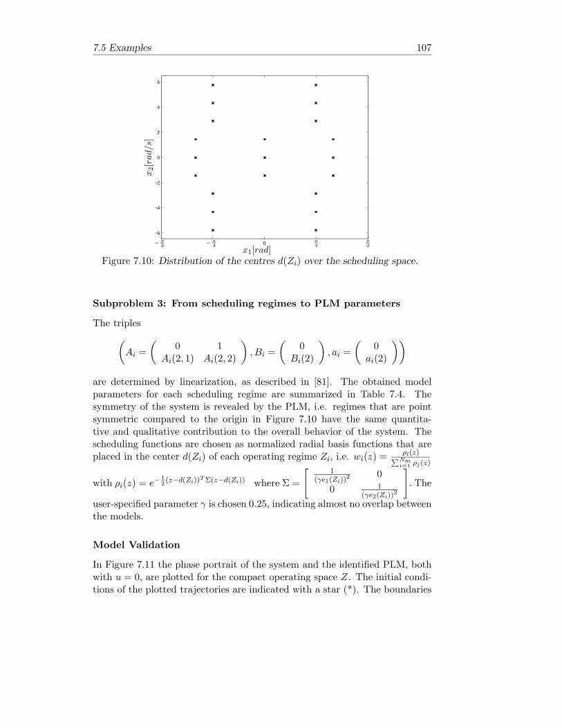
7.5 Examples 107
0
−6
−4
−2
0
2
4
6
x1[rad]
x2[r
ad/s
]
− π2 − π
4π4
π2
Figure 7.10: Distribution of the centres d(Zi) over the scheduling space.
Subproblem 3: From scheduling regimes to PLM parameters
The triples(Ai =
(0 1
Ai(2, 1) Ai(2, 2)
), Bi =
(0
Bi(2)
), ai =
(0
ai(2)
))
are determined by linearization, as described in [81]. The obtained modelparameters for each scheduling regime are summarized in Table 7.4. Thesymmetry of the system is revealed by the PLM, i.e. regimes that are pointsymmetric compared to the origin in Figure 7.10 have the same quantita-tive and qualitative contribution to the overall behavior of the system. Thescheduling functions are chosen as normalized radial basis functions that areplaced in the center d(Zi) of each operating regime Zi, i.e. wi(z) = ρi(z)∑Nm
i=1 ρj(z)
with ρi(z) = e−12(z−d(Zi))
TΣ(z−d(Zi)) where Σ =
[1
(γe1(Zi))2 0
0 1(γe2(Zi))
2
]. The
user-specified parameter γ is chosen 0.25, indicating almost no overlap betweenthe models.
Model Validation
In Figure 7.11 the phase portrait of the system and the identified PLM, bothwith u = 0, are plotted for the compact operating space Z. The initial condi-tions of the plotted trajectories are indicated with a star (*). The boundaries

108 Building PLMs from known Nonlinear Models
of the ellipsoidal validity regions of the operating regimes Zi are also shownby the dotted lines. It is interesting to see how the trajectories are goingthrough the different operating regimes Zi. Almost all of the system trajecto-ries diverge to infinity. The phase portrait shows a saddle point, as indicatedwith the asymptotes along the arrows. As a result in the centre of the plotan unstable equilibrium point can be observed. The difference between thetrajectories of the system and the PLM can be made smaller by repeatingthe procedure for a smaller ε. Qualitatively, the phase portrait of the systemand the PLM are very much alike; the system and the PLM are said to betopological equivalent [60].
0
−6
−4
−2
0
2
4
6
x1[rad]
x2[r
ad/s
]
−π2 −π
4π4
π2
Figure 7.11: Phase portrait of both the system (dashed line) and the PLM(solid line) within the compact scheduling space Z. The dotted ellipsoidalregions centered at d(Zi) are validity regions.
7.6 Notes and Comments
Nonlinearity
Frequently, the term nonlinearity is used in a loose sense when system be-havior is discussed. Think about phrases as: This system is very or stronglynonlinear, or, this system is locally nonlinear. These assertions are often notmade precise, i.e. not supported by mathematical definitions. Within thepresented modelling framework, terms as strongly nonlinear, and locally non-linear, can be given a precise meaning. The decomposition of the system inoperating regimes, allows for an intuitively clear and natural interpretation

7.6 Notes and Comments 109
of these terms. That is, these terms can be qualified and quantified. Next,two definitions are proposed that can contribute to the classification of non-linearities, at least for systems that are defined on a non-compact operatingspace.
Definition 7.6.1 (Locally nonlinear ) A system is locally nonlinear iffor any ε > 0, and for any non-compact operating region, an ε-accurate PLMexists, consisting of a finite number of models.
Definition 7.6.2 (Relatively strongly nonlinear ) A system is rela-tively strongly nonlinear if for any ε > 0 an ε-accurate PLM exists for theregion Ψ such that for some operating region Ψ1 ⊂ Ψ it holds that Nm(Ψ1) !Nm(Ψ) and Ψ1 " Ψ.
Segregation
The segregation procedure relies on a tree construction algorithm for struc-ture optimization. It orthogonally partitions the scheduling space into hyper-rectangles. Similar procedures but for discrete time systems are reported inliterature, see [56] and [34]. A main difference between all these procedures,is the criterion that is used to select the ‘best’ partitioning.

110 Building PLMs from known Nonlinear Models

Chapter 8
Building PLMs fromMeasured Data
8.1 Introduction
As depicted in Figure 6.2, model construction consists of three phases, namelythe selection of a model structure, followed by a model set and finally a modelfrom the model set. Since the model structure is chosen to be a PLM, whatremains to be determined is a model set and the best model has to be selectedfrom the model set. The determination of the model set and a suitable modelfrom the model set depends besides prior knowledge and the type and amountof available data, of course on the objective of modelling.
Two data based modelling methods will be described that automaticallygenerate a PLM from data and prior knowledge. These two methods areoutput error methods, based upon a well known augmented state least squaresfiltering method [22]. A distinction has been made between local and globalparameter estimation methods.
Before presenting the modelling methods, in Section 8.2, the basic aspectsof least squares filtering will be discussed. After that, in Section 8.3, the firstmethod, a local parameter estimation method is presented. It is founded uponthe regime segregation method described earlier. This means that the schedul-ing parameters are identified independently from the local model parameters.In this case the decision to segregate is specified by the output error crite-rion that an augmented state least squares filter tries to minimize. For eachsegregated region, (that is a scheduling regime,) a linear model is estimated.This method is illustrated by an example in Section 8.4. In Section 8.5, thesecond method, a global parameter estimation method is presented. With thesecond method it is shown that it is feasible, at least for small scale problems,to utilize a standard augmented state least squares filter, to estimate for the
111
112 Building PLMs from Measured Data
entire operating space of interest, both the unknown scheduling parametersand the unknown local model parameters simultaneously. This method is il-lustrated by an example in Section 8.6. Finally, in Section 8.7, some notes andcomments are made regarding the proposed methods.
To make the data based modelling methods more clear, first the relevantaspects of least squares filtering will be explained. We will closely follow theformulation presented in [74].
8.2 Least Squares Filtering
In fact, the least squares filter is used as a state reconstruction and parameterestimation method for the determination of the unknown state x and theunknown parameters θ of a continuous time model
x = f(x, u, θ), x(t0) = xt0 (8.1)y = h(x, u, θ)
with state x ∈ Rn, input u ∈ R
m, parameters θ ∈ Rk and output y ∈ R
p. It isthe task of the filtering procedure to estimate the unknowns in some optimalsense given measurements u, yr of the input and the output of the system.The way to formulate and to solve this problem will be outlined below.
By adding a set of k trivial differential equations, θ = 0, to the description(8.1), the combined parameter and state estimation problem is converted intoa pure state reconstruction problem.
x = f(x, u, θ), x(t0) = xt0 (8.2)
θ = 0, θ(t0) = θt0 (8.3)y = h(x, u, θ) (8.4)
Mathematically, the resemblance that exists between the state equation (8.2)and the parameter equation (8.3) clearly suggests that there is no need todistinguish the states x from the parameters θ. Therefore the unknown statex is augmented with the unknown parameters θ, and the new augmented statexa = [xT θT ]T is introduced.
xa = f(xa, u), xa(t0) = xat0 (8.5)y = h(xa, u)
It is assumed that measurements u(t), yr(t) for times t ∈ [t0, te] are avail-able. A model like (8.5) however is only a limited description of reality andthere will always be some discrepancy between the model behavior and the

8.2 Least Squares Filtering 113
measurements. Thus, the measurements will not satisfy (8.5). This discrep-ancy can be taken into account by assuming that the system can be describedby
xa = f(xa, u) + ξ, xa(t0) = xat0 + ζ (8.6)yr = h(xa, u) + η
where ξ(t) and η(t) are called the residuals on the state equation and theoutput equation respectively, and ζ represents the difference between the es-timated initial state xa(t0) and the real initial state xt0 of the system. Ifthe estimate xa is such that the residuals are small in some sense, then thiswill give confidence in the chosen model structure, the measured data andthe obtained estimate. More specifically, optimal filtering refers to the ‘best’estimate xa(t) at the current time t, based upon all past measurements, and isspecified as a least squares estimate xa(t) which minimizes a weighted squaresof the residuals, over the whole interval [t0, t]. For this choice the estimatexa(t) has to minimize the measure
J :=12
∫ t
t=t0
ξ(t)TWξ(t) + η(t)TV η(t)dt +12
ζTR0ζ (8.7)
The matrices W , V and R0 are user specified weighting matrices thatweight the residuals on the state and output equation respectively, they expressconfidence in these equations. As an example, suppose one restricts to modelstructures with constant parameters θ, as is the case in (8.3). By choosing verylarge values for those elements in W that weight the residuals on the parameterequations, it is made sure that the parameter estimates in the augmented statexa will not change significantly with time. In a similar way other prior modelassumptions and knowledge can be incorporated. For instance, the elementsof ξ(t) and ζ(t), besides having different dimensions, often take values thatdiffer substantially from each other in magnitude. Then, such values for theelements in W and V are chosen that the weighted residuals are all of the sameorder of magnitude. After that, to express the confidence we have in certainmodel equations, we can choose larger values for the corresponding elementsin W and V . The matrix W has to be positive definite and V should be asemi-positive definite matrix; often they are chosen diagonal. The column xat0
from ζ = xa(t0)−xat0 represents initial knowledge about the real initial state,and R0 is a positive definite matrix expressing confidence in knowledge of theinitial state.
The optimal estimation or filtering problem is treated extensively in asurvey given in [32] and references therein. An approximate solution xa to the

114 Building PLMs from Measured Data
optimal filtering problem is given by [22]
xa = f(xa, u) + K(yr − h(xa, u)), xa(t0) = xat0 (8.8)
P (t) = F (t)P (t) + P (t)F (t)T
+ W − P (t)H(t)TV −1H(t)P (t), P (t0) = R0 (8.9)
K(t) = P (t)H(t)TV −1 (8.10)
where F = ∂f∂xa
(xa, u) and H = ∂h∂xa
(xa, u), both evaluated at the currentestimated state and current input.
The above filter can also be derived in a statistical setting and interpretedin statistical terms, then called the extended Kalman filter. The state estimateequation (8.8) of the above filter, is nothing more then a copy of the stateequation of the model (8.5), the state of which is improved by taking intoaccount measurements yr of the real system. The measurements are comparedto the output of the model (8.5). The difference between the estimated outputsand the measurements is propagated by the gain matrix K to produce aninnovation signal and to improve the state estimate. The gain K, see (8.9) iscomputed in such a way that it optimally balances the confidence in differentparts of the model, as specified by (8.7).
There is however no guarantee that the approximate filter (8.8,8.9,8.10) willconverge when applied to a system [49]. Nevertheless, in practical applicationthe filter is commonly used, which often leads to useful estimates.
8.3 Local Parameter Estimation
As explained earlier the segregation procedure has as a point of departure themost simple PLM, consisting of only one linear model, which covers the entirescheduling space as depicted in Figure 7.4, and step by step model complexityis increased conceptually as follows: split the nZ dimensional scheduling space‘in the middle’ in two scheduling regimes Zi and Zi+nZ . This can be done innZ different ways, i.e. i = 1, ..nZ. After that a cost criterion is evaluated foreach partitioning, from which the most promising partitioning follows. Onesegregation step is then completed, and segregation is repeated until someprescribed accuracy is achieved, meaning that the criterion that is evaluatedis below some prescribed value.
If there is no model of the system available, the number of models Nm
sufficient to achieve ε-accuracy within some region, cannot be computed andtherefore the suggested criterion for splitting the operating space fails. Auseful criterion however has to measure the distribution of the nonlinearity ofthe system over a grid in the scheduling space.
8.3 Local Parameter Estimation 115
It is assumed that the only information of the system available are measure-ments u, yr of the input u and the output yr, on some time interval [t0, te],and some prior knowledge on the system, such as the order of the system andstructure of the matrices (Ai, Bi, ai, Ci, Di, ci), such as structural zeros andones, involved in the representation of the PLM. The decision to segregate isspecified by the output error criterion that the least squares filter minimizes.For each segregated regime Zi, a linear model (Ai, Bi, ai, Ci, Di, ci), that ispart of the PLM, will be estimated.
8.3.1 Data Based Regime Segregation
The least squares filter (8.8,8.9,8.10) is used as a state reconstruction andparameter estimation method for the determination of the unknown state andthe unknown parameters of the locally valid continuous time models that arepart of the PLM. A locally valid model, i.e. a linear model valid within someregion of the operating space, is described as follows:
x = Aix + Biu + ai, x(t0) = xt0 (8.11)y = Cix + Diu + ci
with state x ∈ Rn, u ∈ R
m and y ∈ Rp. However, in general the state and in
particular the initial state xt0 is unknown, as are some elements θ ∈ Rk of the
matrices Ai, Bi, ..., ci. It is the task of the filter (8.8,8.9,8.10) to estimatethese unknowns.
By adding a set of k trivial differential equations, θ = 0 to the description(8.11), the combined parameter and state estimation problem is converted intoa state reconstruction problem.
x = Ai(θ)x + Bi(θ)u + ai(θ), x(t0) = xt0
θ = 0, θ(t0) = θt0
y = Ci(θ)x + Di(θ)u + ci(θ)
The unknown state x is augmented with the unknown parameters θ, and theaugmented state xa = [xT θT ]T is introduced to obtain (8.5).
First the (optimal) filter (8.8,8.9,8.10) is applied to reconstruct the aug-mented state xa, i.e. the parameters θ and the state x, of the linear model(8.11) based on all the measurements available. Next, the obtained constantparameters θ are substituted in (8.11) and the state x of the model (8.11) isagain reconstructed by a filter. If the underlying nonlinear system is suffi-ciently smooth, then it is expected that within a region small enough, a linearmodel like (8.11) is an acceptable model for the system. Acceptability of the

116 Building PLMs from Measured Data
model (8.11) will be evaluated by a measure similar to (8.7), i.e.
J :=12
∫ t
t=t0
ξ(t)TWξ(t) + η(t)TV η(t)dt +12
ζTR0ζ (8.12)
where ξ(t) = x(t)− Aix(t)−Biu(t)− ai = K(yr(t)− Cix(t)−Diu(t)− ci) isthe filter innovation, η(t) = yr(t)−Cix(t)−Diu(t)− ci the difference betweenthe output of the filter and the measurements, and ζ = x(t0)− xt0 representsuncertainty about the real initial condition. Thus ξ, η and ζ represent errorson the state and output equation due to unmodelled phenomena. A model(8.11) is said to be acceptable if J ≤ ε, with ε > 0 to be specified by theuser. The decision to segregate is specified by a normalized version of (8.12),to account for the time that is spent within some region Zi.
More specifically, we evaluate J(Zi) + J(Zi+nZ ) for all nZ obtained con-figurations, and select the configuration of which the evaluated measure is thesmallest. Here
J(Zi) =1
τ(Zi)
kZi∑j=1
J(Zi, Tj,Zi) (8.13)
J(Zi, Tj,Zi) :=∫t∈Tj,Zi
ξ(t)TWξ(t) + η(t)TV η(t)dt +12
ζTR0ζ (8.14)
were τ(Zi) stands for the time that is spent in region Zi, and Tj,Zi = [t0,j,Zite,j,Zi ] stands for one of the kZi time intervals spent in Zi. Thus
∑kZij=1(te,j,Zi−
t0,j,Zi) = τ(Zi). The situation is depicted in Figure 8.1. Basically, segregationis repeated until for each obtained partitioning J(Zi) ≤ ε. There are how-ever some limitations. If segregation gives no further improvement regardingthe error measure J , in comparison to the error measure of the undividedspace, segregation for that region is stopped. Furthermore, when there arenot enough measurements left to divide, the procedure is stopped. This meansthat either the chosen accuracy, as specified by ε, is too high or the numberof measurements is too small.
For each scheduling regime Zi obtained by segregation, a model (8.1), theset (Ai, Bi, ai, Ci, Di, ci), was already determined by the filter. These modelswill be scheduled by the scheduling functions wi, that are defined as describedin Subsection 7.4, hence the PLM
x =Nm∑i=1
wi(z)Aix + Biu + ai
y =Nm∑i=1
wi(z)Cix + Diu + ci
is specified.
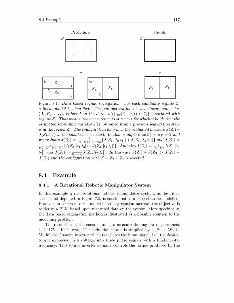
8.4 Example 117
t0t0
t1t2
t3 t4
tete
ZZ
Z1
Z2Z2Z3
Z4Z4
Procedure Result
Figure 8.1: Data based regime segregation. For each candidate regime Zi
a linear model is identified. The parametrization of each linear model, i.e.(Ai, Bi, ..., ci), is based on the data u(t), yr(t) | z(t) ∈ Zi associated withregime Zi. That means, the measurements at times t for which it holds that theestimated scheduling variable z(t), obtained from a previous segregation step,is in the region Zi. The configuration for which the evaluated measure J(Zi)+J(Zi+nZ ) is the smallest is selected. In this example dim(Z) = nZ = 2 andwe evaluate J(Z1) = 1
(t1−t0)+(t4−t3)J(Z1, [t0 t1])+J(Z1, [t3 t4]) and J(Z3) =
1(t3−t1)+(te−t4)
J(Z3, [t1 t3])+J(Z3, [t4 te]). And also J(Z2) = 1(t2−t0)
J(Z2, [t0t2]) and J(Z4) = 1
(te−t2)J(Z4, [t2 te]). In this case J(Z1) + J(Z3) > J(Z2) +
J(Z4) and the configuration with Z = Z2 + Z4 is selected.
8.4 Example
8.4.1 A Rotational Robotic Manipulator System
In this example a real rotational robotic manipulator system, as describedearlier and depicted in Figure 7.5, is considered as a subject to be modelled.However, in contrast to the model based segregation method, the objective isto derive a PLM based upon measured data on the system. More specifically,the data based segregation method is illustrated as a possible solution to themodelling problem.
The resolution of the encoder used to measure the angular displacementis 1.9175 × 10⁻⁴ [rad]. The induction motor is supplied by a ’Pulse WidthModulation’ source inverter which translates the input signal, i.e., the desiredtorque expressed in a voltage, into three phase signals with a fundamentalfrequency. This source inverter actually controls the torque produced by the

118 Building PLMs from Measured Data
motor to the desired torque. The input signal of the source inverter and theTTL encoder signals are respectively sent and read by a dSPACE system [20].During the experiments the sample frequency is set to 1 [kHz].
Prior Knowledge
It is assumed that the robot arm is a nonlinear control affine mechanicalsystem (7.7) with one degree of freedom q, where q represents the angulardisplacement of the arm and u is the input motor voltage. The output y ofthe system is the angular displacement q of the arm.
The mechanical model structure makes it possible to restrict the represen-tation of the PLM by means of structural zeros and ones, i.e.,
Ai =(
0 1Ai(2, 1) Ai(2, 2)
)Bi =
(0
Bi(2)
)ai =
(0
ai(2)
)Ci =
(1 0
)Di = 0 ci = 0
and only the nontrivial parameters, the ones different from 0 and 1 have to beestimated.
From Operating Space to Scheduling Space
The operating space is defined as the product space of the state space withthe input space, i.e. Ψ = X × U where x = [q q]T ∈ X, q ∈ X1, q ∈ X2, andu ∈ U . From Theorem 4.6.3 and the prior knowledge available on the system,we know that it is sufficient to schedule the models over the angle q and angularvelocity q, instead of over all the operating variables q,q and u. This is becausethe variable u enters the model in an affine way. Hence the scheduling spaceZ = X. Theorem 4.6.3 tells us that there will always exist a PLM that achievesarbitrary accuracy, at least if Z is compact and if the system is assumed to besmooth enough. It is expected that the system exhibits nonlinear behavior forlow velocities due to nonlinear friction characteristics. Therefore, it is assumedthat Z = q, q | |q| ≤ π
10 [rad], |q| ≤ 4[rad/s] covers the interesting workingrange of the inverted pendulum.
Experiment Design
First, an experiment has to be designed, i.e. an input signal u has to be ap-plied to the robot arm such that the measurements u, yr contain enoughinformation to determine together with a priori knowledge on the system aPLM that suffices for the modelling task at hand. It is not an easy task to ex-cite the system in the working range of interest. As mentioned earlier, severalcase studies indicated that a relatively high frequency input signal of small

8.4 Example 119
amplitude, superimposed on a low frequency input signal with a relativelylarge amplitude, leads to a data set that contains sufficient information forthe modelling task to be successful. Figure 8.2 shows the data set obtainedfrom the system, that is the input signal together with the output responseof the system. The measurement noise is not visible on the scale of the plot.
0 1 2 3 4 5 6 7 8 9 10−0.2
−0.1
0
0.1
0.2
0 1 2 3 4 5 6 7 8 9 10−0.4
−0.2
0
0.2
0.4
0.6
0.8
1
x1[r
ad]
t [s]
t [s]
u[V
]
Figure 8.2: Experimental data.
The measured angle is differentiated numerically by a zero-phase high passfilter with a cut-off frequency of 200 Hz to reconstruct the angular velocityq. This reconstruction makes it possible to depict the system response in thescheduling space. From Figure 8.3 it can be seen that this trajectory coversthe estimated scheduling space fairly well, which is required for the segrega-tion procedure to work. The reconstructed angular velocity will not be used
−0.3 −0.2 −0.1 0 0.1 0.2 0.3 0.4 0.5 0.6 0.7−5
−4
−3
−2
−1
0
1
2
3
4
x1 = z1 = q[rad]
x2=
z 2=
q[ra
d/s
]
Figure 8.3: System trajectory in the scheduling space Z.

120 Building PLMs from Measured Data
as an additional measurement for the segregation procedure.
Segregation
The data set u, yr is offered to the segregation procedure. The user specifiedaccuracy ε is set as follows, J(Zi) ≤ ε, and the measure J(Zi) is defined in(8.13). Choosing ε = 0.01 we obtain for the segregation method 21 models.
The centres d(Zi) and the widths 2e(Zi) of each operating regime Zi :
d(Zi) − e(Zi) ≤ (z =[
]) ≤ d(Zi) + e(Zi), where d(Zi) =
[d1(Zi)d2(Zi)
]
and e(Zi) =[
e1(Zi)e2(Zi)
]are summarized in Table 8.1. The unknown param-
Table 8.1: Operating regimes and model parameters
i d1(Zi) d2(Zi) e1(Zi) e2(Zi) Ai(2, 1) Ai(2, 2) Bi(2) ai(2)1 0.1683 -2.5673 0.4331 2.1844 -19.6306 -1.3388 474.5737 23.26522 -0.0483 2.8937 0.2165 1.0922 -24.3043 -3.3836 406.8478 -7.01863 -0.0483 1.2554 0.2165 0.5461 -15.0759 -2.9403 369.6105 -5.93024 0.4931 2.8937 0.1083 1.0922 -24.5307 -6.5162 374.8093 1.54095 0.1683 0.2997 0.4331 0.1365 -14.6128 -10.8237 354.7136 -7.48796 0.2224 2.8937 0.0541 1.0922 -20.1223 -4.6237 373.2493 0.28757 0.3307 2.8937 0.0541 1.0922 -25.8769 -3.6231 366.1476 -2.55548 -0.0483 -0.2464 0.2165 0.1365 -21.7033 -9.8994 337.5465 19.81819 0.1683 0.0267 0.4331 0.1365 -12.3130 -41.1949 230.6125 5.4659
10 0.1683 0.5045 0.4331 0.0683 -22.4484 -10.9273 344.9230 -2.827011 0.3307 1.2554 0.0541 0.5461 -24.7331 -6.5735 351.7486 1.667512 0.4931 1.5285 0.1083 0.2731 -23.5115 -9.2669 359.3913 3.134213 0.2765 -0.2464 0.1083 0.1365 -20.1245 -8.6843 338.2395 14.355814 0.1683 0.6069 0.4331 0.0341 -16.7735 -11.4670 332.0291 -2.413415 0.1683 0.6752 0.4331 0.0341 -20.3161 -10.9481 335.3594 -1.228016 0.2224 0.9824 0.0541 0.2731 -21.7525 -8.0048 337.8189 5.092017 0.2224 1.5285 0.0541 0.2731 -22.8421 -9.6383 337.5241 4.374318 0.4931 0.8458 0.1083 0.1365 -25.8317 -11.3728 345.0546 -1.340719 0.4931 1.1189 0.1083 0.1365 -23.5545 -10.6700 343.2975 1.101020 0.4931 -0.3146 0.1083 0.0683 -17.1133 -9.0823 337.7909 13.884521 0.4931 -0.1781 0.1083 0.0683 -15.7904 -8.4212 339.0424 16.1129
eters from Ai =(
0 1Ai(2, 1) Ai(2, 2)
), Bi =
(0
Bi(2)
), ai =
(0
ai(2)
)are determined by the augmented state least squares filter, as a part of thesegregation procedure. The scheduling functions are chosen as normalizedradial basis functions that are placed in the center d(Zi) of each operating
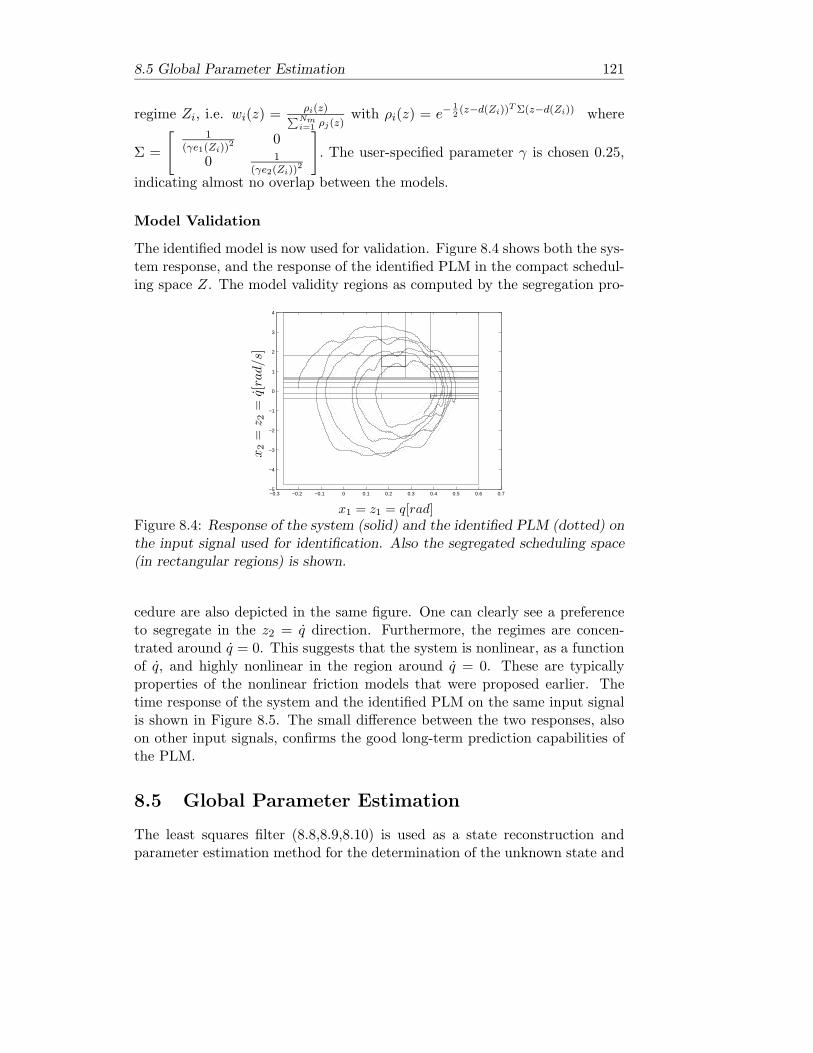
8.5 Global Parameter Estimation 121
regime Zi, i.e. wi(z) = ρi(z)∑Nmi=1 ρj(z)
with ρi(z) = e−12(z−d(Zi))
TΣ(z−d(Zi)) where
Σ =
[1
(γe1(Zi))2 0
0 1(γe2(Zi))
2
]. The user-specified parameter γ is chosen 0.25,
indicating almost no overlap between the models.
Model Validation
The identified model is now used for validation. Figure 8.4 shows both the sys-tem response, and the response of the identified PLM in the compact schedul-ing space Z. The model validity regions as computed by the segregation pro-
−0.3 −0.2 −0.1 0 0.1 0.2 0.3 0.4 0.5 0.6 0.7−5
−4
−3
−2
−1
0
1
2
3
4
x1 = z1 = q[rad]
x2=
z 2=
q[ra
d/s
]
Figure 8.4: Response of the system (solid) and the identified PLM (dotted) onthe input signal used for identification. Also the segregated scheduling space(in rectangular regions) is shown.
cedure are also depicted in the same figure. One can clearly see a preferenceto segregate in the z2 = q direction. Furthermore, the regimes are concen-trated around q = 0. This suggests that the system is nonlinear, as a functionof q, and highly nonlinear in the region around q = 0. These are typicallyproperties of the nonlinear friction models that were proposed earlier. Thetime response of the system and the identified PLM on the same input signalis shown in Figure 8.5. The small difference between the two responses, alsoon other input signals, confirms the good long-term prediction capabilities ofthe PLM.
8.5 Global Parameter Estimation
The least squares filter (8.8,8.9,8.10) is used as a state reconstruction andparameter estimation method for the determination of the unknown state and
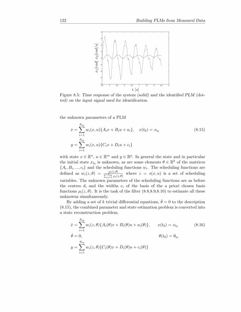
122 Building PLMs from Measured Data
4.5 5 5.5 6 6.5 7 7.5 8 8.5 9−4
−3
−2
−1
0
1
2
3
4
t [s]
x1[r
ad]
x2[r
ad/s
]Figure 8.5: Time response of the system (solid) and the identified PLM (dot-ted) on the input signal used for identification.
the unknown parameters of a PLM
x =Nm∑i=1
wi(x, u)Aix + Biu + ai, x(t0) = xt0 (8.15)
y =Nm∑i=1
wi(x, u)Cix + Diu + ci
with state x ∈ Rn, u ∈ R
m and y ∈ Rp. In general the state and in particular
the initial state xt0 is unknown, as are some elements θ ∈ Rk of the matrices
Ai, Bi, ..., ci and the scheduling functions wi. The scheduling functions aredefined as wi(z, θ) = ρi(z,θ)∑Nm
j=1 ρj(z,θ)where z = s(x, u) is a set of scheduling
variables. The unknown parameters of the scheduling functions are as beforethe centres di and the widths ei of the basis of the a priori chosen basisfunctions ρi(z, θ). It is the task of the filter (8.8,8.9,8.10) to estimate all theseunknowns simultaneously.
By adding a set of k trivial differential equations, θ = 0 to the description(8.15), the combined parameter and state estimation problem is converted intoa state reconstruction problem.
x =Nm∑i=1
wi(z, θ)Ai(θ)x + Bi(θ)u + ai(θ), x(t0) = xt0 (8.16)
θ = 0, θ(t0) = θt0
y =Nm∑i=1
wi(z, θ)Ci(θ)x + Di(θ)u + ci(θ)
8.6 Example 123
The unknown state x is augmented with the unknown parameters θ, and theaugmented state xa = [xT θT ]T is introduced to obtain (8.5).
The optimal filter (8.8,8.9,8.10) is applied to reconstruct the augmentedstate xa, i.e. the parameters θ and the state x, of the PLM (8.15) based on allthe measurements available. Prior system knowledge can be incorporated intothe PLM by restricting the structure, thereby facilitating the applicabilityof the parameter estimation method. Next an experimental case study isreported to illustrate the modelling method, and in particular it is shown howprior knowledge can be incorporated.
8.6 Example
8.6.1 A Rotational Robotic Manipulator System
In this example a real rotational robotic manipulator system, as describedearlier and depicted in Figure 7.5, is considered as a subject for modelling.In conformance with the data based segregation method, the objective is toderive a PLM based upon measured data on the system. More specifically,the global parameter estimation method is illustrated as a possible solution tothe modelling problem.
Prior Knowledge
The state space equations (7.7) describing the robotic manipulator system areassumed to simplify to
d
dt
]=[
q−M−1C(q)
]+[
0M−1Bm
]u
with M the unknown effective inertia of the motor-transmission-rotatingarm combination, Bm = 16 [NmV −1] is the motor gain, and C(q) is thefriction torque. The system is depicted in Figure 7.5. The friction torque is asimplified model of reality, and assumed to be a function of the angular velocityonly. The validity of this assumption is partly confirmed by the outcome ofthe previous example on the subject of data based segregation. There it couldbe seen that segregation dominantly occurred in the q direction. Furthermore,it is assumed that the friction can be modelled by an odd continuous function,i.e.
C(q) = −C(−q)
This is consistent with well known friction models, see Figure 7.6. Forangular velocity equal to zero the model friction torque is zero, which results

124 Building PLMs from Measured Data
in the preservation of equilibrium points of the system. The friction model doesnot describe stiction, since the continuous friction model will always slide (i.e.move) for an applied input u unequal to zero. However if stiction is present inthe system, the stiction regime will be approximated, if the friction functionnear q = 0 is very steep. Then the model can still give acceptable simulationresults, that is angular displacement during stiction will be negligible on ourscale of interest.
The PLM is composed of Nm locally valid models. The structure of eachmodel is chosen equal to the topology of a mechanical system. This makes itpossible to restrict the representation of the PLM, i.e.,
Ai =(
0 10 Ai(2, 2)
)Bi =
(0
Bi(2)
)ai =
(0
ai(2)
)Ci =
(1 0
)Di = 0 ci = 0
and only the nontrivial parameters have to be estimated. With each localmodel (Ai, Bi, ai) a model validity function ρi is associated which, by definitionis close to one for those regions were the corresponding linear model is valid,and zero elsewhere. Here, the validity depends only on the angular velocity q,due to the choice of the nonlinear friction as a function of only q. Hence thescheduling variable z = q. The scheduling functions are defined as normalizedmodel validity functions, i.e. wi(z) = ρi(z)∑Nm
i=1 ρj(z). A typical choice for ρi is the
Gaussian function
ρi(z) = e− (z−d(Zi))2
(2e(Zi))2
where d(Zi) marks the center and 2e(Zi) the width of operating region Zi.The PLM becomes
d
dt
]=
Nm∑i=1
wi(z, θ)Ai(θ) + Bi(θ)u + ai(θ) (8.17)
For the PLM the unknown model parameters that have to be estimated are
θ = [Ai(2, 2), Bi(2), ai(2), d(Zi), e(Zi)]i = 1, ..., Nm
Note that Bi(2) = B(2) = M−1Bm with M unknown. The unknowns θ arefurther reduced by restricting the PLM to construct only odd friction functionsin the following way
• Choose an odd number of local models, i.e. Nm = 2k + 1 with k ∈0, 1, 2, ..., where one local model has no offset, i.e. ai(2) = 0 and thecorresponding center d(Zi) = 0.

8.6 Example 125
• The other Nm−1 models are divided in pairs of two symmetrical aroundz = 0, i.e., the centers are opposite d(Zi) = −d(Zi+1), the widthsare equal e(Zi) = e(Zi+1) as well as the slopes Ai(2, 2) = Ai+1(2, 2)and the offsets are again opposite ai = −ai+1 with i = 2k with k ∈1, 2, ..., 1/2Nm
An advantage of this construction is the reduction of parameters by abouta factor two.
Experiment Design
This same data set was used as for the data based segregation method (seeFigure 8.2).
Filtering
The augmented state least squares filter (8.8,8.9,8.10) was implemented off-line. For the PLM the number Nm is set to three, in order to facilitate theestimation procedure. If this PLM does not lead to a satisfactory model, thencomplexity can be increased gradually by increasing Nm.
In this case θ = [A1(2, 2), e(Z1), A2(2, 2), a2(2), d(Z2), e(Z2), M ], i.e. 7 pa-rameters have to be determined; 6 for the friction model and the inertia M .The filter parameters R0, W, V from (8.8,8.9,8.10), which express consecutivelyconfidence or uncertainty in initial states, model equations and measurementshave to be tuned in order to obtain reliable augmented state estimates. Theinitial state x of the system is known, but the model parameters θ are notknown. The initial model parameters are chosen in such a manner that phys-ical known properties, e.g., positive inertia value or positive viscous dampervalue, are met. (Though we have no guarantee that that will stay that way dur-ing the estimation phase.) Hence, the uncertainty for the initial state estimatesis small while we are not sure of the initial estimates for the model parameters.These considerations lead to the initial augmented state uncertainty matrixR0 = diag(0, 0, 1, . . . , 1) where the non-zero elements express the uncertaintyof initially uncertain parameters. The matrix W can be seen as expressinguncertainty on the augmented state model equations. The model equationsdescribing constant model parameters θ = 0 and d
dtq = q are regarded astrue. The confidence in these equations being large, is expressed by a zero atthe corresponding places at the diagonal matrix W = diag(0, W22, 0, . . . , 0).Here Q22 = 0.001 expresses uncertainty in the proposed friction model. Dueto the finite encoder resolution of 1.9175 10−4 [rad] and the differentiationscheme an uncertainty on the angular velocity reconstruction is introduced.To take this into account the matrix V is constructed as a diagonal matrixV = diag(0.001, 0.01) where 0.001 corresponds to the uncertainty in the angle

126 Building PLMs from Measured Data
measurement and 0.01 to the uncertainty in the arm velocity reconstruction.The filter tuning is mainly based on experience and trial and error. It is impor-tant that the parameters converge to constant values. Different filter tuningwill result in different convergence speeds and even parameter divergence canoccur. The estimated data are passed through the filter several times until theparameter estimates converge. After 10 filter passes the parameter estimatesbecome constant and the sum of eigenvalues of the covariance matrix P (t)has become minimal. The identified inertia value is M = 0.0323 [kgm2rad−1].The obtained model parameters for each scheduling regime Zi are summarizedin Table 8.2. The scheduling functions are shown in Figure 8.6.
Table 8.2: Operating regimes and model parameters
i d(Zi) e(Zi) Ai(2, 2) Bi(2) ai(2)1 0 0.0290 −2040.3 495.7782 02 1.6162 1.4033 −2.2466 495.7782 18.70123 1.6162 1.4033 −2.2466 495.7782 −18.7012
−5 −4 −3 −2 −1 0 1 2 3 4 50
0.5
1
−5 −4 −3 −2 −1 0 1 2 3 4 50
0.5
1
−5 −4 −3 −2 −1 0 1 2 3 4 50
0.5
1
w2
w1
w3
Scheduling functions
x2 = z2 = q[rad/s]Figure 8.6: The scheduling functions w1, w2, and w3.
Model Validation
The identified model is now used for validation. Figure 8.7 shows the timeresponse of the system and of the identified PLM. An input signal similar tothe one used for identification purposes is applied.
The identified friction torque of the PLM with superimposed on it thescaled Kalman filter innovation signal (dotted line) is depicted in Figure 8.8.

8.7 Notes and Comments 127
4.5 5 5.5 6 6.5 7 7.5 8 8.5 9−4
−3
−2
−1
0
1
2
3
4
t [s]
x1[r
ad]
x2[r
ad/s
]
Figure 8.7: Time response of the system (solid) and the identified PLM (dot-ted) on the input signal used for identification.
The innovation is small and seems random and therefore gives no furtherinformation on how to improve the friction characteristic of the PLM. Fromthis observation together with the fact that the filtered output and even thesimulated output is very close to the system, it is concluded that the modelcaptures the main nonlinearity of the system.
Coulomb, viscous and Stribeck friction phenomena can be observed anddistinguished from the estimated friction model. The PLM can be interpretedin terms of regimes as follows. Regimes Z2, Z3 and the associated models areresponsible for the viscous friction part. Regime Z1 and the associated modelis responsible for the Coulomb part. The non-empty intersection of the regionsZ1, Z2 and Z3 and the associated convex combination of the associated modelsis responsible for the Stribeck part of the friction.
8.7 Notes and Comments
Least squares filtering
The least squares filtering toolbox, which includes simulation and validationfacilities, that was used throughout this chapter for the estimation of un-known parameters, is available as a non-commercial Matlab toolbox with auser friendly graphical interface [26].
In principle, the presented second modelling method could be applied on-line in real time applications.
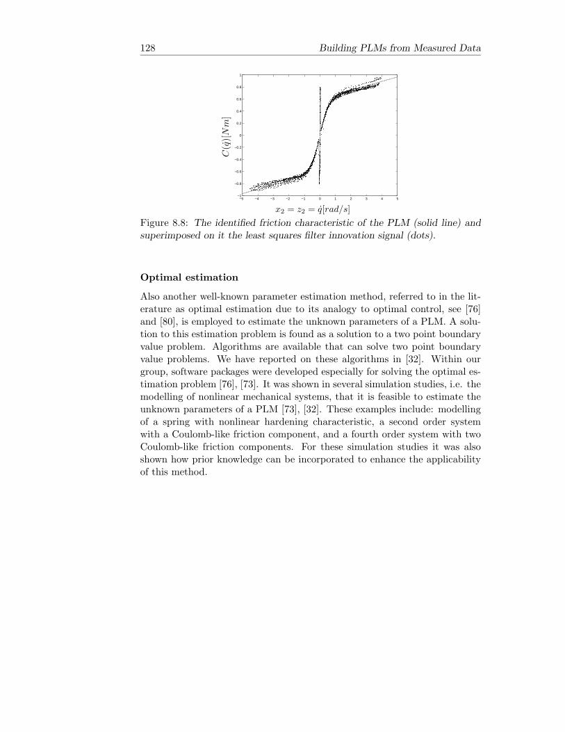
128 Building PLMs from Measured Data
−5 −4 −3 −2 −1 0 1 2 3 4 5−1
−0.8
−0.6
−0.4
−0.2
0
0.2
0.4
0.6
0.8
1
C(q
)[N
m]
x2 = z2 = q[rad/s]Figure 8.8: The identified friction characteristic of the PLM (solid line) andsuperimposed on it the least squares filter innovation signal (dots).
Optimal estimation
Also another well-known parameter estimation method, referred to in the lit-erature as optimal estimation due to its analogy to optimal control, see [76]and [80], is employed to estimate the unknown parameters of a PLM. A solu-tion to this estimation problem is found as a solution to a two point boundaryvalue problem. Algorithms are available that can solve two point boundaryvalue problems. We have reported on these algorithms in [32]. Within ourgroup, software packages were developed especially for solving the optimal es-timation problem [76], [73]. It was shown in several simulation studies, i.e. themodelling of nonlinear mechanical systems, that it is feasible to estimate theunknown parameters of a PLM [73], [32]. These examples include: modellingof a spring with nonlinear hardening characteristic, a second order systemwith a Coulomb-like friction component, and a fourth order system with twoCoulomb-like friction components. For these simulation studies it was alsoshown how prior knowledge can be incorporated to enhance the applicabilityof this method.