Tanveer, Gauntlett, Diaz, Yeh

Design of a Flight Planning System to Reduce

Persistent Contrail Formation to Reduce

Greenhouse Effects

Harris Tanveer

David Gauntlett

Jhonnattan Diaz

Paul Yeh

Department of Systems Engineering and Operations Research

George Mason University

Fairfax, VA 22030-4444

April 23, 2014

SYST 495

Final Report

2

Table of Contents

1.0 Context ...................................................................................................................................... 5

1.1 Global Climate Change ......................................................................................................... 5

1.2 Air Travel Demand ............................................................................................................... 6

1.3 Aircraft Emissions ................................................................................................................ 7

1.3.1 Carbon Dioxide .............................................................................................................. 8

1.3.2 Contrails ....................................................................................................................... 10

1.4 Possible Contrail Mitigation Options.................................................................................. 13

1.4.1 Jet Fuel Additives ........................................................................................................ 13

1.4.2 Jet Engine Redesign ..................................................................................................... 14

1.4.3 Operational Changes to Flight Planning ...................................................................... 14

1.5 Air Traffic Control .............................................................................................................. 15

2.0 Stakeholder Analysis .............................................................................................................. 16

2.1 Stakeholders ........................................................................................................................ 16

2.1.1 Federal Aviation Administration- Air Traffic Organization ........................................ 16

2.1.2 Airlines- Airline Management ..................................................................................... 16

2.1.3 Citizens and Climate Change Advocates ..................................................................... 17

2.1.4 International Civil Aviation Organization (ICAO) ...................................................... 17

2.2 Tensions Amongst Stakeholders ......................................................................................... 17

2.3 Win-Win Analysis .............................................................................................................. 20

3.0 Gap Analysis ........................................................................................................................... 23

3.1 Projected RF from Contrails ............................................................................................... 23

3.2 The Tradeoff ....................................................................................................................... 24

4.0 Need and Problem ................................................................................................................... 25

5.0 Project Scope .......................................................................................................................... 26

5.1 Altitude ............................................................................................................................... 26

5.2 Contrail Type ...................................................................................................................... 26

5.3 Strategic vs. Tactical Maneuvering ..................................................................................... 26

5.4 Regions with High Likelihood of Contrails ........................................................................ 26

5.4.1 NOAA Weather Data- Binary Contrail Formation in ISSR ........................................ 26

3

5.4.2- Geographic Scope ....................................................................................................... 29

5.5 FAA Enhanced Traffic Management System (ETMS) ....................................................... 29

6.0 Functional Requirements ........................................................................................................ 30

6.1 Requirement Hierarchies .................................................................................................... 30

6.2 Requirements Outline ......................................................................................................... 40

7.0 Functional Decomposition ...................................................................................................... 44

8.0 Method of Analysis ................................................................................................................. 54

8.1 Design Alternatives ............................................................................................................. 54

8.2 Design of Experiment ......................................................................................................... 55

9.0 Simulation Design ................................................................................................................... 56

9.1 Simulation Elements ........................................................................................................... 56

9.1.1 Simulation Controller................................................................................................... 56

9.1.2 Flight Object ................................................................................................................ 58

9.1.3 Flight Database Handler .............................................................................................. 58

9.1.4 Weather Database Handler .......................................................................................... 59

9.1.5 Great Circle Distance Router ....................................................................................... 59

9.2 System Inputs ...................................................................................................................... 59

9.2.1 Weather Input............................................................................................................... 59

9.2.2 Aircraft Information ..................................................................................................... 60

9.2.3 Flight Plan Data ........................................................................................................... 60

9.3 Contrail Avoidance Algorithm ........................................................................................... 61

9.4 System Outputs ................................................................................................................... 63

9.4.1 Distance Flown ............................................................................................................ 63

9.4.2 Distance of Contrails Produced ................................................................................... 63

9.4.3 Fuel Burn ..................................................................................................................... 63

9.4.4 Kilograms CO2 Produced ............................................................................................ 63

9.4.5 Radiative Forcing from Contrails ................................................................................ 63

9.4.6 Radiative Forcing from CO2 ....................................................................................... 64

9.5 Physical Processes Modeled ............................................................................................... 65

9.5.1 𝑪𝑶𝟐 Emission Model .................................................................................................. 65

9.5.2 Contrail Formation Model ........................................................................................... 65

4

11.0 Project Management ............................................................................................................. 66

11.1 Budgeting .......................................................................................................................... 71

10.2 Work Breakdown Structure and Schedule ........................................................................ 73

12.0 References ............................................................................................................................. 77

5

1.0 Context

1.1 Global Climate Change

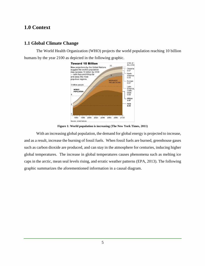
The World Health Organization (WHO) projects the world population reaching 10 billion

humans by the year 2100 as depicted in the following graphic.

Figure 1: World population is increasing (The New York Times, 2011)

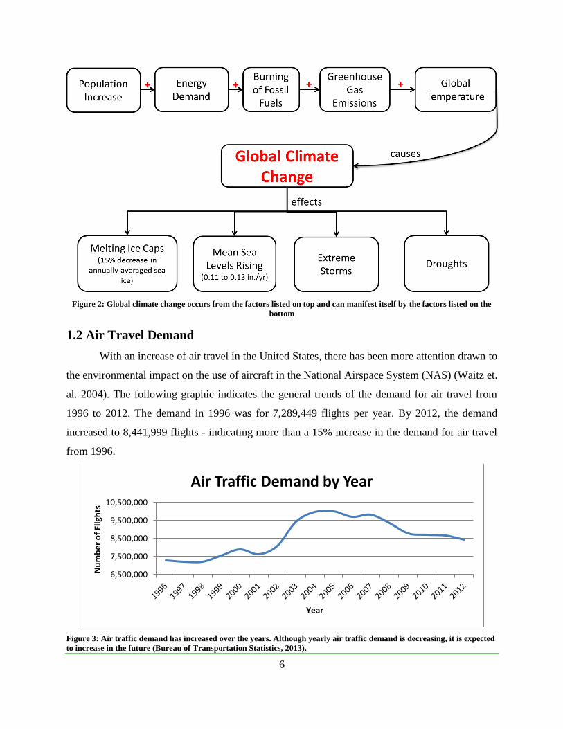
With an increasing global population, the demand for global energy is projected to increase,

and as a result, increase the burning of fossil fuels. When fossil fuels are burned, greenhouse gases

such as carbon dioxide are produced, and can stay in the atmosphere for centuries, inducing higher

global temperatures. The increase in global temperatures causes phenomena such as melting ice

caps in the arctic, mean seal levels rising, and erratic weather patterns (EPA, 2013). The following

graphic summarizes the aforementioned information in a causal diagram.

6

Figure 2: Global climate change occurs from the factors listed on top and can manifest itself by the factors listed on the

bottom

1.2 Air Travel Demand

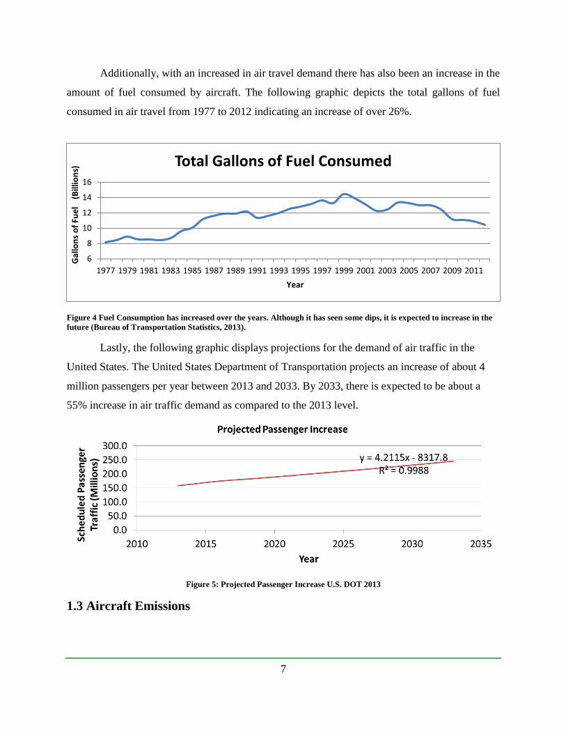
With an increase of air travel in the United States, there has been more attention drawn to

the environmental impact on the use of aircraft in the National Airspace System (NAS) (Waitz et.

al. 2004). The following graphic indicates the general trends of the demand for air travel from

1996 to 2012. The demand in 1996 was for 7,289,449 flights per year. By 2012, the demand

increased to 8,441,999 flights - indicating more than a 15% increase in the demand for air travel

from 1996.

Figure 3: Air traffic demand has increased over the years. Although yearly air traffic demand is decreasing, it is expected

to increase in the future (Bureau of Transportation Statistics, 2013).

6,500,000

7,500,000

8,500,000

9,500,000

10,500,000

Nu

mb

er

of

Flig

hts

Year

Air Traffic Demand by Year

7

Additionally, with an increased in air travel demand there has also been an increase in the

amount of fuel consumed by aircraft. The following graphic depicts the total gallons of fuel

consumed in air travel from 1977 to 2012 indicating an increase of over 26%.

Figure 4 Fuel Consumption has increased over the years. Although it has seen some dips, it is expected to increase in the

future (Bureau of Transportation Statistics, 2013).

Lastly, the following graphic displays projections for the demand of air traffic in the

United States. The United States Department of Transportation projects an increase of about 4

million passengers per year between 2013 and 2033. By 2033, there is expected to be about a

55% increase in air traffic demand as compared to the 2013 level.

Figure 5: Projected Passenger Increase U.S. DOT 2013

1.3 Aircraft Emissions

6

8

10

12

14

16

1977 1979 1981 1983 1985 1987 1989 1991 1993 1995 1997 1999 2001 2003 2005 2007 2009 2011

Gal

lon

s o

f Fu

el

(Bill

ion

s)

Year

Total Gallons of Fuel Consumed

8

The process of the combustion of jet fuel produces carbon dioxide, sulfur oxides, soot,

hydrocarbons, and nitrogen oxides. The following graphic denotes the chemical changes involved

in the combustion process of Jet A fuel.

Figure 6: Jet A fuel combustion process (Sridhar, 2011)

From the above graphic, the impacts of aircraft emissions can create global climate effects

in terms of changes in temperature. The effect of aircraft emissions on the Earth’s climate is one

of the most anthropogenic long-term environmental issues facing the aviation industry (IPCC,

2004). Estimates show that aviation is responsible for 13% of transportation-related fossil fuel

consumption and 2% of all anthropogenic CO2 emissions (Minnis, 2005). The transportation

industry as an entirety is responsible for 28% of CO2 emissions in the United States.

1.3.1 Carbon Dioxide

The increase of Green House Gas (GHG) emissions contributes to global warming through

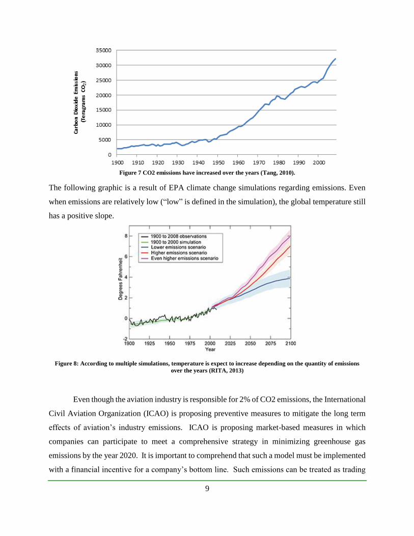
the greenhouse effects (Nolan, 2010). According to the following image, carbon dioxide emissions

from fossil fuels increase exponentially from 1900 to 2008. Understanding this growth paves the

foundation to understanding the magnitude and impact on global climate. Carbon dioxide creates

a net warming effect on the planet.

H2O"

Air'

Fuel'

SOx'

HC'

Soot'

H2O" Aerosols'

Contrails"

NOx'

CO2"

CH4'

O2'

Jet'A'Fuel'Combus8on'Process'

Sridhar,'Banavar'&'Chen,'Neil.'“Design'of'Aircra: 'Trajectories'based'on'Trade/offs'between'Emission'Sources.”'2011.'

Aircra: 'Engine'

Chemical'Reac8ons'

Microphysical'Processes'

Climate'Change'through'Radia8ve'Forcing'

aCnH2n+2'+'bO2'+'3.76bN2'→'cH2O'+'dCO2'+'3.76bN2'+'heat'

9

Figure 7 CO2 emissions have increased over the years (Tang, 2010).

The following graphic is a result of EPA climate change simulations regarding emissions. Even

when emissions are relatively low (“low” is defined in the simulation), the global temperature still

has a positive slope.

Figure 8: According to multiple simulations, temperature is expect to increase depending on the quantity of emissions

over the years (RITA, 2013)

Even though the aviation industry is responsible for 2% of CO2 emissions, the International

Civil Aviation Organization (ICAO) is proposing preventive measures to mitigate the long term

effects of aviation’s industry emissions. ICAO is proposing market-based measures in which

companies can participate to meet a comprehensive strategy in minimizing greenhouse gas

emissions by the year 2020. It is important to comprehend that such a model must be implemented

with a financial incentive for a company’s bottom line. Such emissions can be treated as trading

10

commodities in order to achieve the objective of long term, cost effective, and implementation of

environmental progress (EPA, 2013).

1.3.2 Contrails

In 1992, linear condensation-trails, otherwise known as contrails, were estimated to cover

about 0.1% of the Earth’s surface (ICAO, 2010). The contrail cover was projected to grow to 0.5%

by 2050. Contrails contribute to warming the Earth’s surface, similar to thin cirrus clouds formed

in the troposphere and have an important environmental impact because they artificially increase

the cloud cover and trigger the formation of cirrus clouds; thus altering climate on both, local and

global scales (Heymsfield, 2010).

Persistent contrails form cirrus clouds made of water vapor from engine exhaust or the

aerodynamics of a jet aircraft. Whether or not contrails will be persistent is specified through the

Schmidt-Appleman criterion. At cruising altitudes (between 21,000 feet and 41,000 feet) with

temperature below -40oC and where the relative humidity with respect to ice RHi is greater than

100%, the exhaust mixture freezes, forming ice particles upon contact with the free air, leading to

visible contrail formation. Areas where the RHi exceeds 100% are known as Ice Supersaturated

Regions (Schumann, 2005). Generally, contrails created through the aerodynamics of an aircraft

fade within two to three wingspans of an aircraft. Persistent contrails that occur in ISSR can have

lifetimes ranging from 20 minutes to 3 hours can extend an average of 400 kilometers in length

(Schumann 2011).

Persistent contrails are believed to be responsible for the incremental increase of trapped

solar radiation in the earth’s surface, which contributes to the effect of global warming. Recent

reports state that persistent contrails may have a three to four times greater effect on the climate

than carbon dioxide emissions in a short time horizon of 10 to 20 years (Travis, 2004). Greenhouse

gasses are in the atmosphere for longer periods of time relative to contrails therefore allowing the

gasses to mix in the atmosphere, having the same concentration throughout the world. Contrails

on the other hand, provide more regional affects since they occur only in select areas of the

troposphere that fulfill the conditions for persistent contrail formation (Tang, 2010).

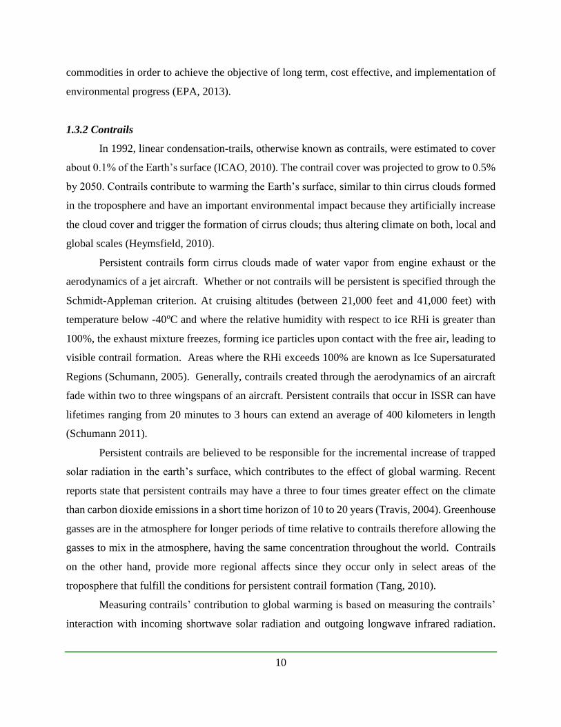
Measuring contrails’ contribution to global warming is based on measuring the contrails’

interaction with incoming shortwave solar radiation and outgoing longwave infrared radiation.

11

This interaction of radiation with contrails creates a net imbalance of energy, known as radiative

forcing (Lee, 2009).

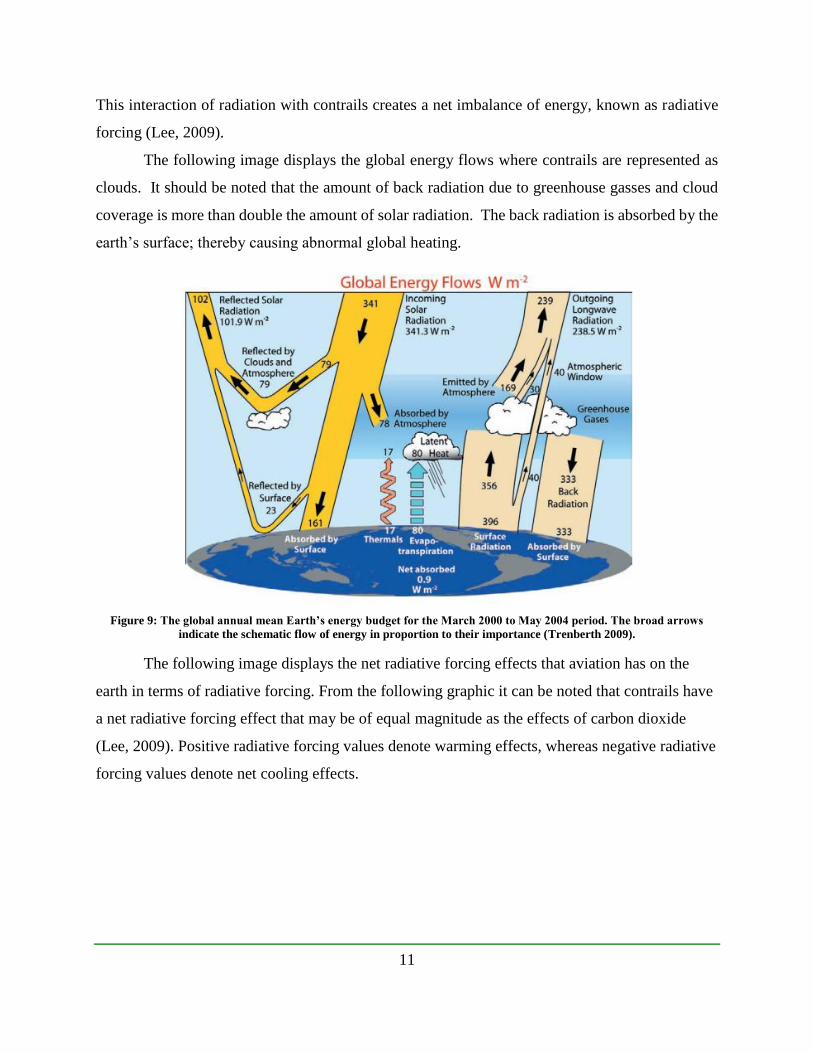
The following image displays the global energy flows where contrails are represented as

clouds. It should be noted that the amount of back radiation due to greenhouse gasses and cloud

coverage is more than double the amount of solar radiation. The back radiation is absorbed by the

earth’s surface; thereby causing abnormal global heating.

Figure 9: The global annual mean Earth’s energy budget for the March 2000 to May 2004 period. The broad arrows

indicate the schematic flow of energy in proportion to their importance (Trenberth 2009).

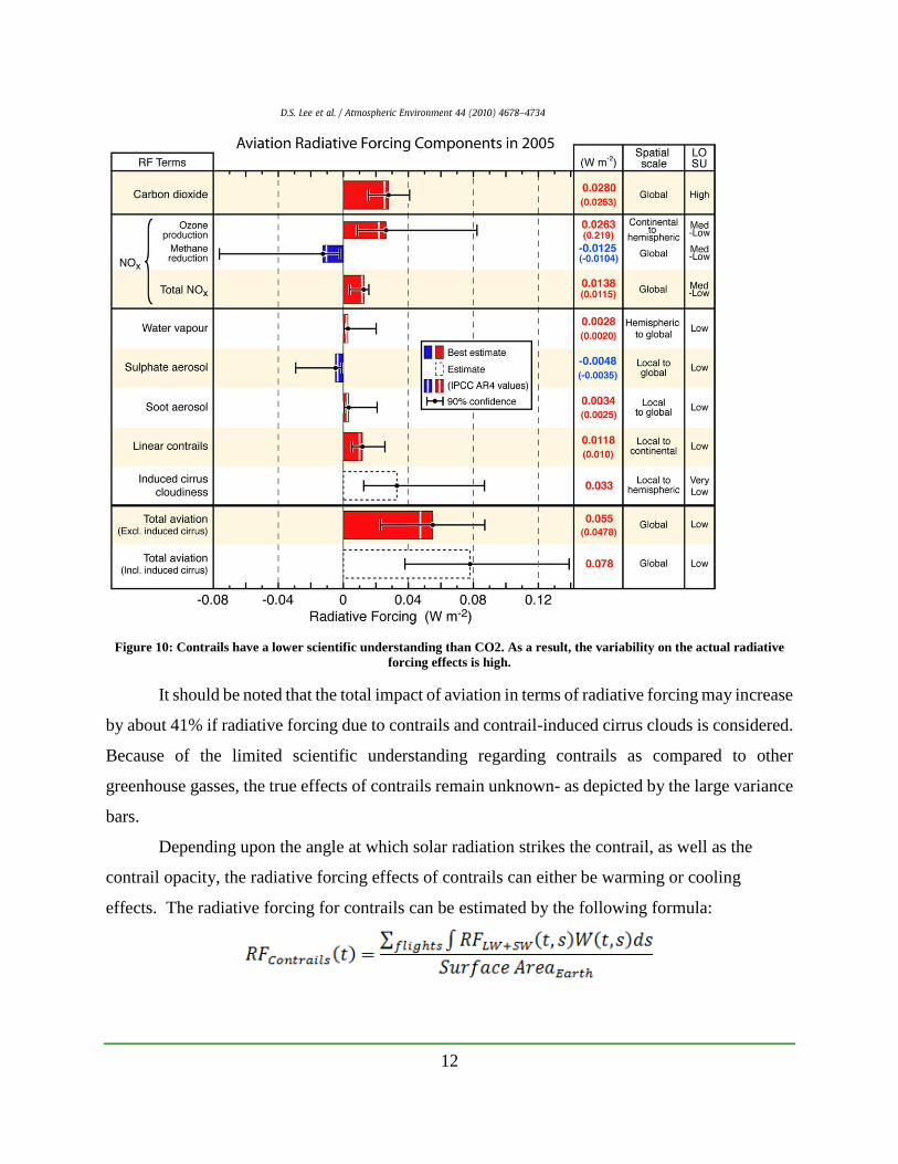
The following image displays the net radiative forcing effects that aviation has on the

earth in terms of radiative forcing. From the following graphic it can be noted that contrails have

a net radiative forcing effect that may be of equal magnitude as the effects of carbon dioxide

(Lee, 2009). Positive radiative forcing values denote warming effects, whereas negative radiative

forcing values denote net cooling effects.

12

Figure 10: Contrails have a lower scientific understanding than CO2. As a result, the variability on the actual radiative

forcing effects is high.

It should be noted that the total impact of aviation in terms of radiative forcing may increase

by about 41% if radiative forcing due to contrails and contrail-induced cirrus clouds is considered.

Because of the limited scientific understanding regarding contrails as compared to other

greenhouse gasses, the true effects of contrails remain unknown- as depicted by the large variance

bars.

Depending upon the angle at which solar radiation strikes the contrail, as well as the

contrail opacity, the radiative forcing effects of contrails can either be warming or cooling

effects. The radiative forcing for contrails can be estimated by the following formula:

13

The RFLW and RFSW terms measure the longwave and shortwave radiative forcing. The longwave

and shortwave radiative forcing term is multiplied by the contrail width and integrated across

space. The entire integration is summed over the number of flights and divided by the surface

area of the earth.

1.4 Possible Contrail Mitigation Options

Methods for contrail mitigation include using fuel that requires lower freezing points than

Jet A-fuel, designing engines that reduce

1.4.1 Jet Fuel Additives

The formation of contrails occurs when hot engine exhaust mixes with ambient temperature

and humidity. As aforementioned, the decomposition of jet emissions consists of carbon dioxide

(CO2), nitrogen oxides (NOx), sulfur oxide (SO2), soot, and water particle (H2O). At cruising

altitudes, the exhaust mixture freezes and forms ice particles upon contact with the surrounding

air. This leads to the formation of visible contrails. The number of ice particles formed in contrails

may be reduced by lowering soot emissions and sulfur content of aviation fuels. However, the

efficiency of such a measure has not yet been quantified (Travis, 2004). Jet fuel additives provide

the optimal ratio of Sulfur (S) content mixture within jet fuel (CnHm+S) during the jet fuel

combustion in order to product an ideal combustion that will reduce contrail formation.

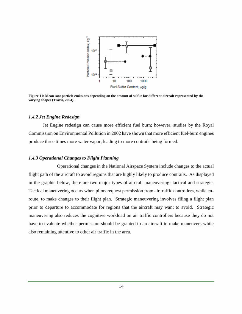
The following figure shows the number of soot and ice particle per kilogram of fuel in

contrails versus fuel sulfur content (FSC) behind the following aircraft: ATTAS (black squares),

B737 (black circles), and A310 (black diamonds). The symbols with dashed lines approximate the

mean soot particle emission indices measured for three aircraft in non-contrail plumes. The grey

rectangles with error bars denote the number of ice particle formed per kg of fuel burned in contrail

for B737 and the ATTAA (Travis, 2004).

14

Figure 11: Mean soot particle emissions depending on the amount of sulfur for different aircraft represented by the

varying shapes (Travis, 2004).

1.4.2 Jet Engine Redesign

Jet Engine redesign can cause more efficient fuel burn; however, studies by the Royal

Commission on Environmental Pollution in 2002 have shown that more efficient fuel-burn engines

produce three times more water vapor, leading to more contrails being formed.

1.4.3 Operational Changes to Flight Planning

Operational changes in the National Airspace System include changes to the actual

flight path of the aircraft to avoid regions that are highly likely to produce contrails. As displayed

in the graphic below, there are two major types of aircraft maneuvering- tactical and strategic.

Tactical maneuvering occurs when pilots request permission from air traffic controllers, while en-

route, to make changes to their flight plan. Strategic maneuvering involves filing a flight plan

prior to departure to accommodate for regions that the aircraft may want to avoid. Strategic

maneuvering also reduces the cognitive workload on air traffic controllers because they do not

have to evaluate whether permission should be granted to an aircraft to make maneuvers while

also remaining attentive to other air traffic in the area.

15

Figure 12: Operational changes due to ISSRs

Furthermore, from the graphic displayed in figure 12, ISSR, or areas with RHi > 100% can

be treated as areas of bad weather that must be avoided. Therefore, as opposed to flying through

those regions as the red dotted line in Figure 12 indicates, the aircraft can fly with the blue dotted

line to avoid the ISSR.

1.5 Air Traffic Control

The Federal Aviation Administration has designated Federal Airways (FARs) that can be

decomposed into the categories of Very High Frequency (VHF) Omnidirectional Range (VOR),

and Colored Airways. The latter is only used in Canada, Alaska, and coastal areas. VORs on the

other hand, are predominately used within the continental United States and were established in

1950’s for aviation navigation (FAA, 2013).

VORs are subdivided into low altitude designated (Victor airways) areas that covers the

range of air space between 1,200 - 17,999 feet above Mean Sea Level (MSL) classification, and

Class A airspace covering high altitude Jet Routes between 18,000 – 45,000 feet above MSL.

While in cruise altitude, aircraft will be passing through different VORs along their destination

until they start the arrival descent towards the airport through the Terminal Radar Approach

Control (TRACON) (FAA, 2013).

16

2.0 Stakeholder Analysis

The motivation for this project is the scarcity of the National Air Space (NAS) due to the

increasing demand for air travel (Bureau of Transportation Statistics, 2013). After careful

consideration and strenuous research for designing a system to manage and create new flight, the

group has identified the stakeholders that will be involved and will be impacted with the

implementation of a flight planning system to reduce persistent contrail formation. The primary

stakeholders are the Federal Aviation Administration (more specifically the Air Traffic

Organization department), airline management for airlines utilizing the NAS, the consumers of air

travel, and other citizens concerned about climate change.

2.1 Stakeholders

The following is a description of key stakeholders impacted by the flight planning system.

2.1.1 Federal Aviation Administration- Air Traffic Organization

Under the umbrella of the Federal Aviation Administration (FAA), there is a complex

network of departments that exist for the operations of everyday commercial aviation in the

National Airspace System (NAS). A major component of this network is composed of the Air

Traffic Organization (ATO), which operates facilities such as Air Traffic Control System

Command Centers (ATSCC), Air Route Traffic Control Centers (ARTCCs), Terminal Radar

Approach Control Facilities (TRACONs), and Air Traffic Control Towers (ATCTs). The branches

of the ATO are necessary to perform essential services starting from the flight plan to the takeoff

of the aircraft following through all the way to the final descent of the aircraft. The primary

objective of the ATO and all its branches is to ensure safe and efficient transportation in the

increasing density of the National Airspace System (Nolan, 2010).

2.1.2 Airlines- Airline Management

Although it is in the best interest of an airline to provide users (customers) with safe

transportation, airlines are in the business of making a profit. Their primary concern is to provide

customers with faster flight times at lower operational costs. At the same time, for the continuity

of operation, airlines are subjected to regulations set forth by the FAA.

17

2.1.3 Citizens and Climate Change Advocates

Because the effects of condensation trails exist mainly on a regional level, citizens and

climate change advocates may be concerned about the net heating conditions in their particular

areas contributing to global warming. Additionally, with the rerouting of aircraft, citizens may be

concerned with pollution from aircraft flying over their region and possibly increasing noise

pollution.

2.1.4 International Civil Aviation Organization (ICAO)

The International Civil Aviation Organization (ICAO) is an agency developed by the

United Nations that sets standards and regulations for the safety and efficiency of international air

space. Currently, the ICAO is comprised of 191 countries that promote security and environmental

protection all around the world.

Apart from the safety and efficiency objectives, another main goal of the ICAO is to

develop a sustainable business model that would enable it to construct a policy framework that

would impart a systematic strategy for a sustainable enterprise. This is an important aspect given

the trends of rising oil prices, rising demand for air travel, and rising operating cost for airline

companies.

The ICAO also promotes environmental policies taking into consideration technological

factors pertaining engine emissions. ICAO is mitigating these problems by restructuring

operational procedures, and the aid of financial tools that can create possibilities of moving

towards a carbon market based trading market.

2.2 Tensions Amongst Stakeholders

The primary goal of the ATO is to maintain a determined level of safety for the successful

air travel operations within the National Airspace System. The airline management’s main goal is

to maintain financial viability while satisfying user demand. Additionally, customers

(citizens/public) demand safe transportation, with minimal monetary costs for air transportation,

while taking into consideration environmental conservation (Nolan, 2010).

18

Although there is a high degree of communication and collaboration amongst these

stakeholders, undoubtedly there will be conflicts along the workings of all operational agencies

that encompass the model of transporting passengers safely, efficiently, and in an environmentally

conscious manner in order to come up with a cohesive solution to the problem of contrail

neutrality.

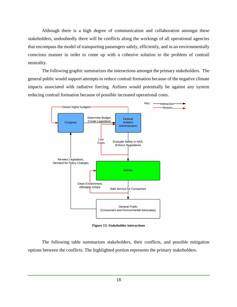
The following graphic summarizes the interactions amongst the primary stakeholders. The

general public would support attempts to reduce contrail formation because of the negative climate

impacts associated with radiative forcing. Airlines would potentially be against any system

reducing contrail formation because of possible increased operational costs.

Figure 13: Stakeholder interactions

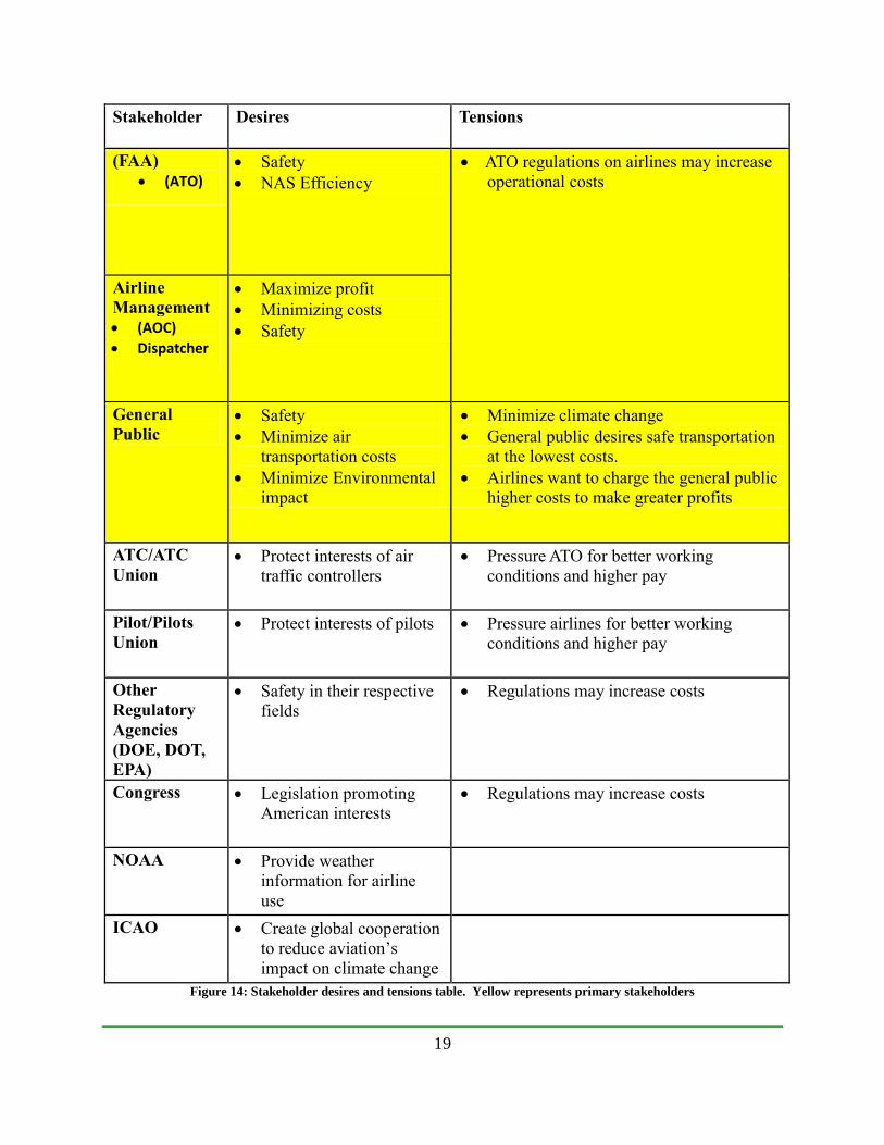
The following table summarizes stakeholders, their conflicts, and possible mitigation

options between the conflicts. The highlighted portion represents the primary stakeholders.

19

Stakeholder Desires Tensions

(FAA)

(ATO) Safety

NAS Efficiency

ATO regulations on airlines may increase

operational costs

Airline

Management

(AOC)

Dispatcher

Maximize profit

Minimizing costs

Safety

General

Public Safety

Minimize air

transportation costs

Minimize Environmental

impact

Minimize climate change

General public desires safe transportation

at the lowest costs.

Airlines want to charge the general public

higher costs to make greater profits

ATC/ATC

Union Protect interests of air

traffic controllers

Pressure ATO for better working

conditions and higher pay

Pilot/Pilots

Union Protect interests of pilots Pressure airlines for better working

conditions and higher pay

Other

Regulatory

Agencies

(DOE, DOT,

EPA)

Safety in their respective

fields

Regulations may increase costs

Congress Legislation promoting

American interests

Regulations may increase costs

NOAA Provide weather

information for airline

use

ICAO Create global cooperation

to reduce aviation’s

impact on climate change

Figure 14: Stakeholder desires and tensions table. Yellow represents primary stakeholders

20

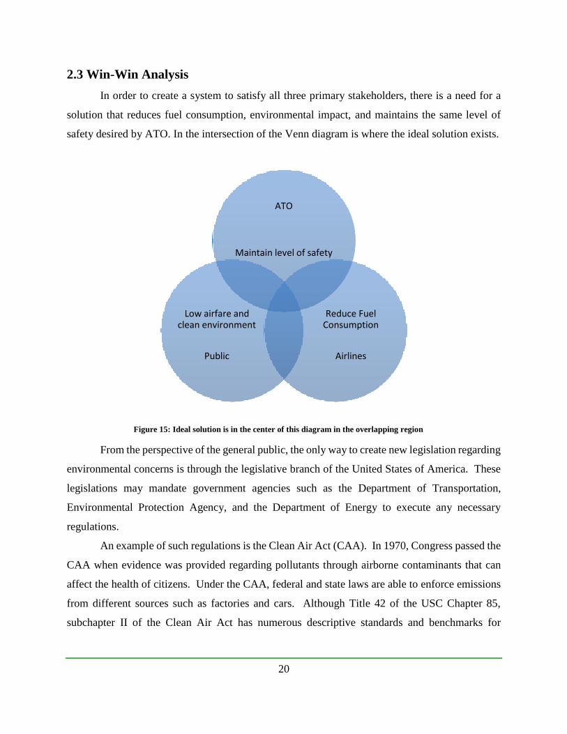
2.3 Win-Win Analysis

In order to create a system to satisfy all three primary stakeholders, there is a need for a

solution that reduces fuel consumption, environmental impact, and maintains the same level of

safety desired by ATO. In the intersection of the Venn diagram is where the ideal solution exists.

Figure 15: Ideal solution is in the center of this diagram in the overlapping region

From the perspective of the general public, the only way to create new legislation regarding

environmental concerns is through the legislative branch of the United States of America. These

legislations may mandate government agencies such as the Department of Transportation,

Environmental Protection Agency, and the Department of Energy to execute any necessary

regulations.

An example of such regulations is the Clean Air Act (CAA). In 1970, Congress passed the

CAA when evidence was provided regarding pollutants through airborne contaminants that can

affect the health of citizens. Under the CAA, federal and state laws are able to enforce emissions

from different sources such as factories and cars. Although Title 42 of the USC Chapter 85,

subchapter II of the Clean Air Act has numerous descriptive standards and benchmarks for

ATO

Maintain level of safety

Reduce Fuel Consumption

Airlines

Low airfare and clean environment

Public

21

emissions for motor vehicles, the broad language and vague delineation of aircraft emission

standards has left the aviation industry with very little current emission regulations (Nolan, 2010).

Because aircraft emissions are a global problem, organizations such as the International

Civil Aviation Organization (ICAO) aim to create cooperative decisions on a global scale. In

2008, the European Union (EU) decided to independently regulate greenhouse gas emissions from

aircraft by means of an Emission Trade System (ETS) in order to decrease the CO2 emissions

produced by all aircraft leaving and entering the EU. By 2012, president Obama and Congress

signed a law prohibiting any type of participation of any EU mandates. As it is becoming apparent,

there is a lack of uniformity of who should regulate greenhouse gasses and how regulations would

be mandated and implemented throughout the globe. This realization is the main objective of the

win-win situation for the stakeholders (specially the airline industry) in the Design of a Flight

Planning System to Reduce Persistent Contrail Formation.

In creating such a system, legislation can be enacted to regulate standards for new engines,

existing engines, airframes, as well as operational standards. For new technology, the innovation

of engine design and airframes will deliver efficiency and close the gap of greenhouse gas

emissions. However, for existing aircraft engines, the continued level of fuel burn will hinder the

goal of carbon neutrality.

Operational standards provide a cost effective and rapid incorporation of testing that will

be beneficial as a first step approach to greenhouse gas emissions. Another aspect is to promote

regulatory tools such as Carbon Emission Trading that will allow the EPA to regulate emissions,

and move towards a system that would be uniform in conjunction with measures taken by the EU

and in the near future (2020) to be adopted around the world with the facilitation of the ICAO

(Richardson, 2013).

Adopting and enforcing rigid guidelines and regulations from the federal government on

airlines will impose great compliance costs (such as increased fuel costs) not only on airlines, but

regulatory agencies, and the general public demanding environmental change by means of taxes

and tariffs. As economists are studying different alternatives, they are in consensus that a less rigid,

and more “flexible” approach to this issue would enable the stakeholders to gradually adapt to a

new system. Economists have been studying the European Union’s ETS and can see the value on

emissions trading as the best cost effective for all parties to adopt. Because aviation’s

environmental impact is global, airlines have to become more open to the idea of environmental

22

responsibility as a whole, and economists believe that the most cost-conscious approach to flexible

regulation will be a market-based economy based on the global trade of pollutants (Richardson,

2013).

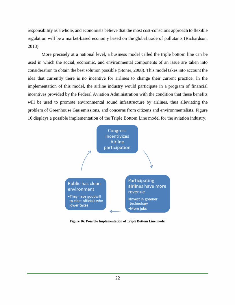
More precisely at a national level, a business model called the triple bottom line can be

used in which the social, economic, and environmental components of an issue are taken into

consideration to obtain the best solution possible (Stoner, 2008). This model takes into account the

idea that currently there is no incentive for airlines to change their current practice. In the

implementation of this model, the airline industry would participate in a program of financial

incentives provided by the Federal Aviation Administration with the condition that these benefits

will be used to promote environmental sound infrastructure by airlines, thus alleviating the

problem of Greenhouse Gas emissions, and concerns from citizens and environmentalists. Figure

16 displays a possible implementation of the Triple Bottom Line model for the aviation industry.

Figure 16: Possible Implementation of Triple Bottom Line model

23

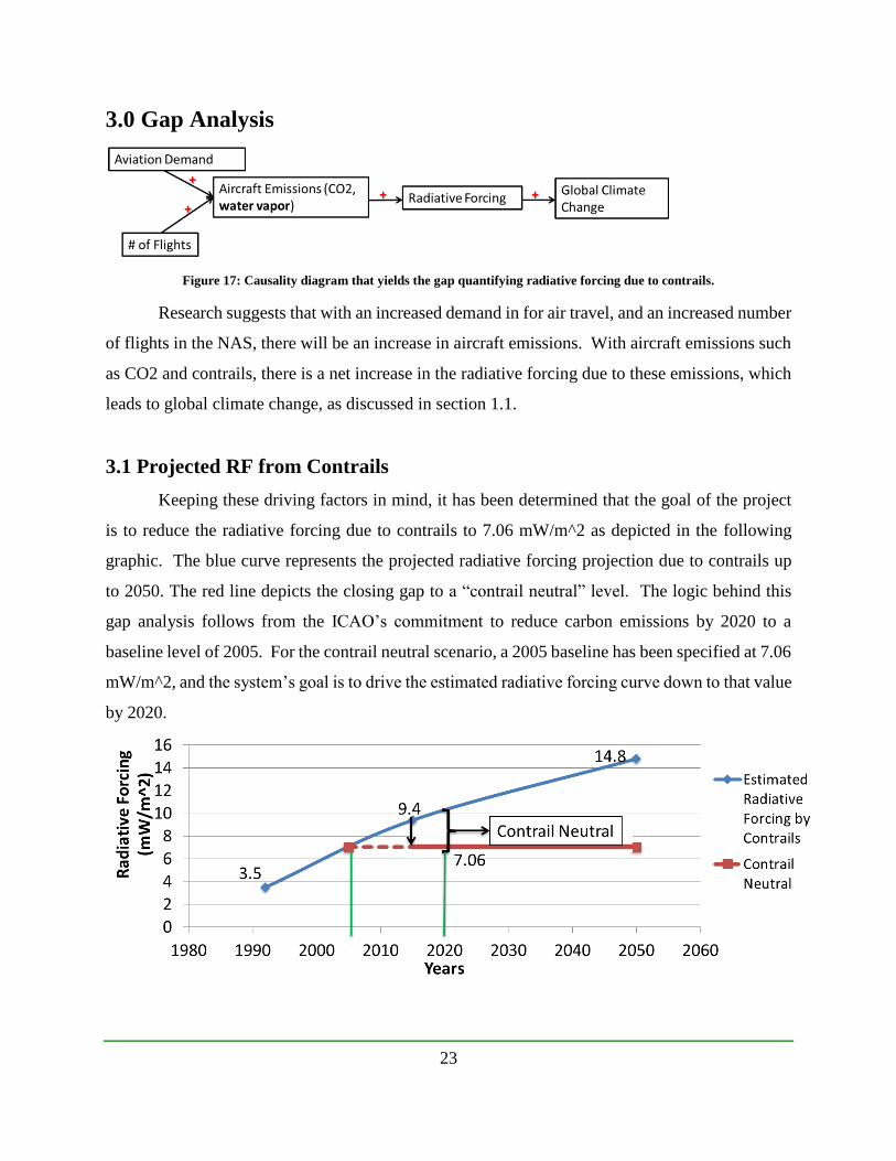
3.0 Gap Analysis

Figure 17: Causality diagram that yields the gap quantifying radiative forcing due to contrails.

Research suggests that with an increased demand in for air travel, and an increased number

of flights in the NAS, there will be an increase in aircraft emissions. With aircraft emissions such

as CO2 and contrails, there is a net increase in the radiative forcing due to these emissions, which

leads to global climate change, as discussed in section 1.1.

3.1 Projected RF from Contrails

Keeping these driving factors in mind, it has been determined that the goal of the project

is to reduce the radiative forcing due to contrails to 7.06 mW/m^2 as depicted in the following

graphic. The blue curve represents the projected radiative forcing projection due to contrails up

to 2050. The red line depicts the closing gap to a “contrail neutral” level. The logic behind this

gap analysis follows from the ICAO’s commitment to reduce carbon emissions by 2020 to a

baseline level of 2005. For the contrail neutral scenario, a 2005 baseline has been specified at 7.06

mW/m^2, and the system’s goal is to drive the estimated radiative forcing curve down to that value

by 2020.

24

In order to decrease the amount of radiative forcing due to contrails, the system would have

to decrease the miles of contrails that are produced as the aircraft travels through ISSR. Decreasing

the miles of contrails decreases the percentage of contrail coverage over the NAS, which would

then decrease the effects of radiative forcing from contrails.

3.2 The Tradeoff

Although avoiding ISSR will decrease the radiative forcing due to contrails, it will

increase the distance the aircraft has to travel, the radiative forcing due to carbon dioxide, the

fuel consumption, as well as the CO2 emissions. Therefore, a method was created for this project

to determine the RF due to carbon dioxide versus the RF due to contrails for a given flight path.

The radiative forcing due to contrails is based off of the interaction of contrails with the

solar zenith angle, the contrail opacity, as well as the ambient temperature. The formula is

described in section 1.3.2. The RF due to contrails would then be dependent upon the length of

the contrails from the proportion of the distance that the aircraft traversed ISSR.

The radiative forcing due to CO2 is assessed by determining the proportion of the global

contribution of CO2 the flight path makes, multiplied by CO2’s global radiative forcing. For

example, in 2005, aviation contributed about 641 Tg of CO2, and about 30 mW/m^2 for

radiative forcing (Lee, 2009). The radiative forcing due to excess CO2 can be determined by

25

4.0 Need and Problem

With an increase in the demand for air travel resulting in the environmental impacts

discussed in the Context Analysis, there is also a need for determining flight paths to reduce the

amount of persistent contrails that can form. Currently there is no existing system that provides

flight paths for aircraft to avoid Ice Super saturated Regions (ISSR) while accounting for the

tradeoffs between fuel consumption, the amount of time aircraft are in the air, as well as the miles

of contrails that are formed by ISSR avoidance flight plans.

In order to solve the problem of radiative heating due to contrails, the ultimate goal of the

project is to design a system for the user to create a flight plan that reduces persistent contrail

formation while taking into consideration the tradeoffs of fuel consumption, the radiative forcing

due to contrails, as well as the radiative forcing due to carbon dioxide emissions.

26

5.0 Project Scope

The complex problem of contrail reduction has been scoped to a manageable scale with

certain assumptions being made. The assumptions include locations of contrail formation, flight

levels of aircraft, as well as flight timings.

5.1 Altitude

The range of altitude of the study has been scoped to flight levels 267 – 414. The

methodology of range are based on average cruising altitude for commercial aviation jets, and

because contrails have a higher likelihood of formation due to atmospheric temperatures being

below -40 degrees Celsius. The limit on height is due to the ceiling of many commercial aircraft

such as the Boeing 737 being at 41,000 feet.

5.2 Contrail Type

The project scope will be limited only to contrails formed by the exhaust of jet engines,

excluding contrails originated by the aerodynamics of jet aircraft. Unlike water vapor exhaust that

can form persistent contrails, aerodynamic contrails are not persistent and dissipate within 2 to 3

wingspans behind the aircraft.

5.3 Strategic vs. Tactical Maneuvering

The methodology of our project has projected two viable solutions for the analysis of

contrail formation due to ISSRs. The first is strategic maneuvering, which consists on preflight

plans that have been approved by the flight dispatcher taking into consideration the weather data

from NOAA, thus knowing where the ISSRs are and planning accordingly. The second is tactical

maneuvering where actual changes in flight paths are done depending if the conditions of ISSR

are present. The recommendation is to research strategic preflight plans for contrail reduction in

contrast to tactical maneuvering.

5.4 Regions with High Likelihood of Contrails

5.4.1 NOAA Weather Data- Binary Contrail Formation in ISSR

27

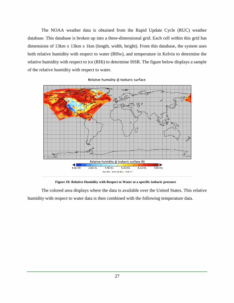
The NOAA weather data is obtained from the Rapid Update Cycle (RUC) weather

database. This database is broken up into a three-dimensional grid. Each cell within this grid has

dimensions of 13km x 13km x 1km (length, width, height). From this database, the system uses

both relative humidity with respect to water (RHw), and temperature in Kelvin to determine the

relative humidity with respect to ice (RHi) to determine ISSR. The figure below displays a sample

of the relative humidity with respect to water.

Figure 18: Relative Humidity with Respect to Water at a specific isobaric pressure

The colored area displays where the data is available over the United States. This relative

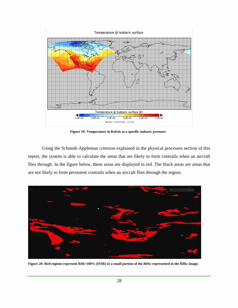
humidity with respect to water data is then combined with the following temperature data.

28

Figure 19: Temperature in Kelvin at a specific isobaric pressure

Using the Schmidt-Appleman criterion explained in the physical processes section of this

report, the system is able to calculate the areas that are likely to form contrails when an aircraft

flies through. In the figure below, these areas are displayed in red. The black areas are areas that

are not likely to form persistent contrails when an aircraft flies through the region.

Figure 20: Red regions represent RHi>100% (ISSR) in a small portion of the RHw represented in the RHw image.

29

This study will assume binary contrail formation. Anytime the RHi is at least 100% an ISSR will

be created. The assumption is that contrails will always be formed in that region.

5.4.2- Geographic Scope

Because of the availability of RUC data, the project was scoped to the Continental United

States (CONUS). The specific flight levels taken into account in this system are 267, 283, 301,

320, 341, 363, 387, and 414. The reason of scoping to only 8 flight levels is also based on the

availability of RUC data. Lastly, radiative forcing was calculated only through deterministic

quantities because of the lack of data available to create a stochastic environment.

5.5 FAA Enhanced Traffic Management System (ETMS)

The system will run a simulation based on 24 hours of flight data obtained from FAA’s

Enhanced Traffic Management System (ETMS) database. The system will use this flight data to

test 45 different days of weather conditions. By using the same flight data, the system is able to

just test the effects of different weather on the total miles of contrails formed, the amount of fuel

used by each aircraft, as well as the flight duration and carbon dioxide emissions.

30

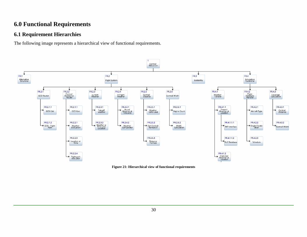
6.0 Functional Requirements

6.1 Requirement Hierarchies

The following image represents a hierarchical view of functional requirements.

Figure 21: Hierarchical view of functional requirements

31

The simulation’s top level requirement states that the system shall reduce the amount of

contrails, measured by area covered, produced by commercial aircraft flying domestically in the

United States. In order to fulfill this high-level requirement, the simulation is decomposed into

four functional requirements. Some of these functional requirements are broken down further. The

hierarchy below shows this breakdown.

Moving from left to right, the contrail reduction requirement is decomposed into the

alternative solutions, flight system, traceability, and simulation controller requirements. The

alternative solutions requirement states that the system shall be able to accept any alternate solution

in order to produce measurable results. The flight system requirement states that the system shall

be able to accept a flight input from a user, and return the miles/width of contrails formed as well

as the extra fuel needed for contrail avoidance. The scalability requirement requires that the system

shall be scalable- in other words, it will be able to run using multiple cores. This will ensure that

the simulation can be used to test various solutions while maintaining a large sample size. Lastly,

the simulation controller requirement states that the simulation shall contain a “controller” that

handles all of the timing and any calculations external to the flight object. Both, the flight system

and simulation requirements, are broken down into sub requirements that will be explained further.

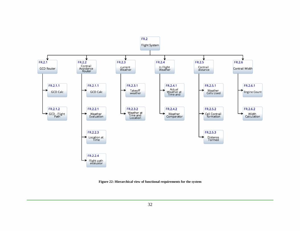
The flight system breakdown, seen on the next page, contains all of the requirements

necessary to meet fulfill the flight system requirement.

32

Figure 22: Hierarchical view of functional requirements for the system

33

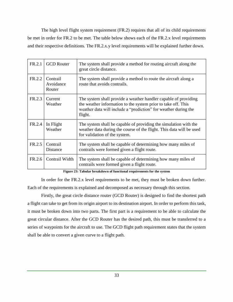
The high level flight system requirement (FR.2) requires that all of its child requirements

be met in order for FR.2 to be met. The table below shows each of the FR.2.x level requirements

and their respective definitions. The FR.2.x.y level requirements will be explained further down.

FR.2.1 GCD Router The system shall provide a method for routing aircraft along the

great circle distance.

FR.2.2 Contrail

Avoidance

Router

The system shall provide a method to route the aircraft along a

route that avoids contrails.

FR.2.3 Current

Weather

The system shall provide a weather handler capable of providing

the weather information to the system prior to take off. This

weather data will include a “prediction” for weather during the

flight.

FR.2.4 In Flight

Weather

The system shall be capable of providing the simulation with the

weather data during the course of the flight. This data will be used

for validation of the system.

FR.2.5 Contrail

Distance

The system shall be capable of determining how many miles of

contrails were formed given a flight route.

FR.2.6 Contrail Width The system shall be capable of determining how many miles of

contrails were formed given a flight route.

Figure 23: Tabular breakdown of functional requirements for the system

In order for the FR.2.x level requirements to be met, they must be broken down further.

Each of the requirements is explained and decomposed as necessary through this section.

Firstly, the great circle distance router (GCD Router) is designed to find the shortest path

a flight can take to get from its origin airport to its destination airport. In order to perform this task,

it must be broken down into two parts. The first part is a requirement to be able to calculate the

great circular distance. After the GCD Router has the desired path, this must be transferred to a

series of waypoints for the aircraft to use. The GCD flight path requirement states that the system

shall be able to convert a given curve to a flight path.

34

Figure 24: Requirements for GCD Router

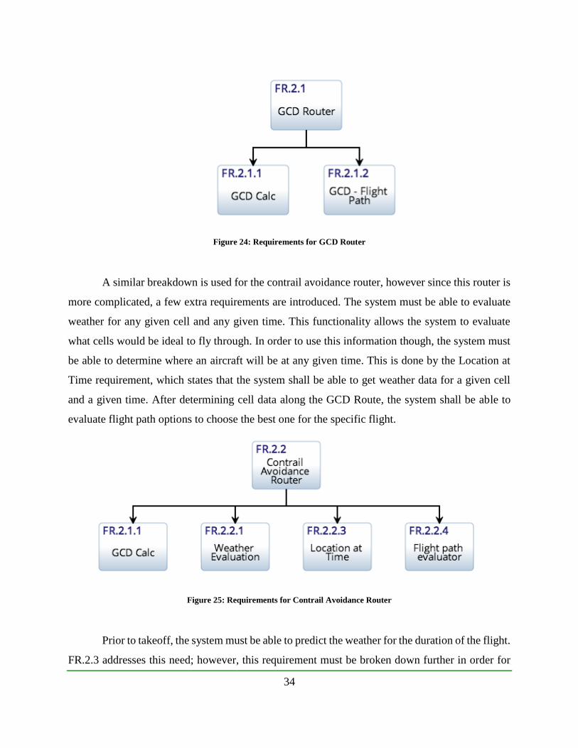
A similar breakdown is used for the contrail avoidance router, however since this router is

more complicated, a few extra requirements are introduced. The system must be able to evaluate

weather for any given cell and any given time. This functionality allows the system to evaluate

what cells would be ideal to fly through. In order to use this information though, the system must

be able to determine where an aircraft will be at any given time. This is done by the Location at

Time requirement, which states that the system shall be able to get weather data for a given cell

and a given time. After determining cell data along the GCD Route, the system shall be able to

evaluate flight path options to choose the best one for the specific flight.

Figure 25: Requirements for Contrail Avoidance Router

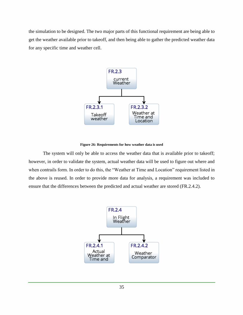
Prior to takeoff, the system must be able to predict the weather for the duration of the flight.

FR.2.3 addresses this need; however, this requirement must be broken down further in order for

35

the simulation to be designed. The two major parts of this functional requirement are being able to

get the weather available prior to takeoff, and then being able to gather the predicted weather data

for any specific time and weather cell.

Figure 26: Requirements for how weather data is used

The system will only be able to access the weather data that is available prior to takeoff;

however, in order to validate the system, actual weather data will be used to figure out where and

when contrails form. In order to do this, the “Weather at Time and Location” requirement listed in

the above is reused. In order to provide more data for analysis, a requirement was included to

ensure that the differences between the predicted and actual weather are stored (FR.2.4.2).

36

Figure 27: Requirements for how weather data is used

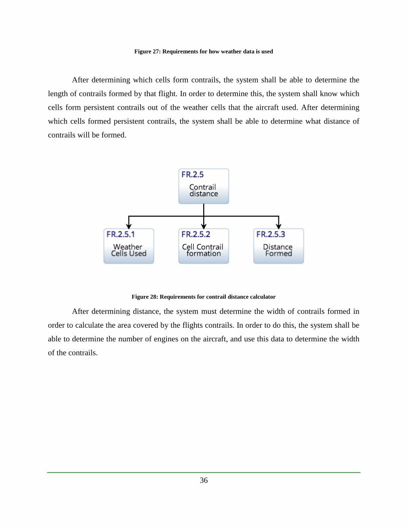
After determining which cells form contrails, the system shall be able to determine the

length of contrails formed by that flight. In order to determine this, the system shall know which

cells form persistent contrails out of the weather cells that the aircraft used. After determining

which cells formed persistent contrails, the system shall be able to determine what distance of

contrails will be formed.

Figure 28: Requirements for contrail distance calculator

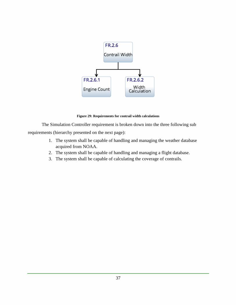
After determining distance, the system must determine the width of contrails formed in

order to calculate the area covered by the flights contrails. In order to do this, the system shall be

able to determine the number of engines on the aircraft, and use this data to determine the width

of the contrails.

37

Figure 29: Requirements for contrail width calculations

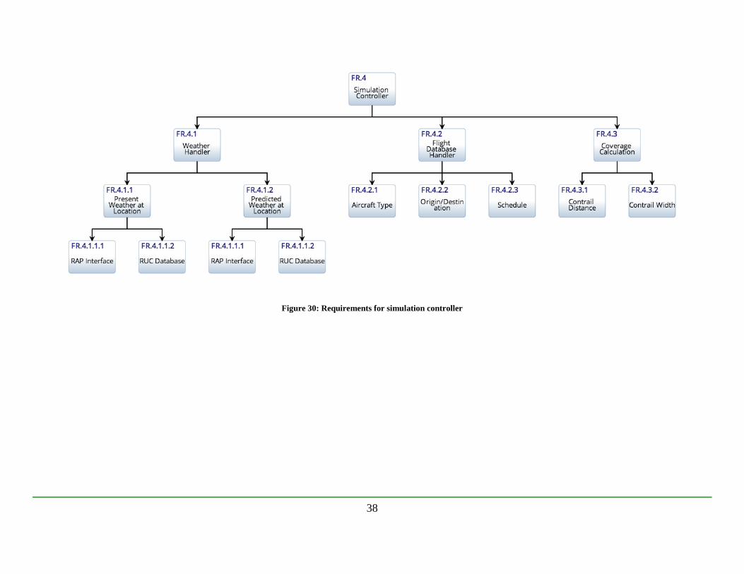
The Simulation Controller requirement is broken down into the three following sub

requirements (hierarchy presented on the next page):

1. The system shall be capable of handling and managing the weather database

acquired from NOAA.

2. The system shall be capable of handling and managing a flight database.

3. The system shall be capable of calculating the coverage of contrails.

38

Figure 30: Requirements for simulation controller

39

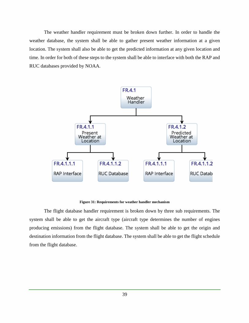
The weather handler requirement must be broken down further. In order to handle the

weather database, the system shall be able to gather present weather information at a given

location. The system shall also be able to get the predicted information at any given location and

time. In order for both of these steps to the system shall be able to interface with both the RAP and

RUC databases provided by NOAA.

Figure 31: Requirements for weather handler mechanism

The flight database handler requirement is broken down by three sub requirements. The

system shall be able to get the aircraft type (aircraft type determines the number of engines

producing emissions) from the flight database. The system shall be able to get the origin and

destination information from the flight database. The system shall be able to get the flight schedule

from the flight database.

40

Figure 32: Requirements for flight database handler mechanism

In order to fulfill the requirement to calculate contrail coverage, the system shall be able to

calculate and sum the contrail distance formed from the flights. The system must also be able to

calculate the width of contrails, and how many miles of each width were formed.

Figure 33: Requirements for contrail coverage calculations

6.2 Requirements Outline

The following is an outline of all the requirements presented above.

1. Alternative Solutions: The simulation shall be able to accept any of the alternative solutions

in order to produce a result.

41

2. Flight System: Each system designed shall accept a flight, and return an amount of extra fuel

needed and miles of contrails formed.

2.1. GCD Router: The system shall provide a method for routing aircraft along the great

circle distance.

2.1.1. GCD Calc: The system shall be capable of calculating the great circle distance

given any two points on a sphere.

2.1.2. GCD - Flight Path: The system shall be capable of forming a flight path from the

calculated great circle distance.

2.2. Contrail Avoidance Router: The system shall provide a method to route the aircraft

along a route that avoids contrails.

2.2.1. Weather Evaluation: The system shall be able to determine which cells of air must

be avoided based on a given time.

2.2.2. GCD Calc: The system shall be capable of calculating the great circle distance

given any two points on a sphere.

2.2.3. Location at time: The system shall be able to determine what location it will be at

for any given time during the flight. Will be based off of the flight path up to that

point.

2.2.4. Flight path evaluator: The system shall be able to compare weather to avoid, as

well as the GCD route in order to determine the best route to take.

2.3. Current Weather: The system shall provide a weather handler capable of providing the

weather information to the aircraft before takeoff.

2.3.1. Takeoff Weather: The system shall be capable of providing the weather

information to the system that is available prior to takeoff.

2.3.2. Weather at time and location: Given a time, and cell the weather handler shall be

able to return a predicted weather, with statistics.

2.4. In flight weather: The system shall be capable of providing the simulation with the

weather data during the course of the flight.

2.4.1. Actual weather at time and location: The system shall be capable of getting the

actual weather data for a specific cell at a certain time.

2.4.2. Weather Comparator: The system shall be able to compare the actual weather to

the predicted weather in order to determine the accuracy of the system

42

2.5. Contrail distance: The system shall be capable of determining which weather cells the

aircraft flew through, and for how many miles the aircraft was in each cell.

2.5.1. Weather Cells used: The system shall be capable of determining which weather

cells the aircraft flew through, and for how many miles the aircraft was in each cell.

2.5.2. Cell contrail formation: Given a cell and weather information, the system shall be

able to determine the probability of persistent contrails being formed.

2.5.3. Distance formed: Given the cells, and contrail formation methods, the system

shall be able to determine the miles of contrails formed by a specific flight.

2.6. Contrail width: The system shall be capable fo returning the width of contrails formed

by the aircraft during its flight.

2.6.1. Engine Count: Given the flight information, the system shall be able to determine

how many engines the aircraft has.

2.6.2. Width Calculation: Given the number of engines, and any other necessary aircraft

information, the system shall be able to determine the width of contrails formed by

the flight.

3. Scalability: The simulation shall be scalable via threading.

4. Simulation Controller: The system shall be able to manage and control a simulation in order

to gather test and reliability results.

4.1. Weather Handler: The system shall be able to handle the weather database in order to

provide the necessary information to flight planner and simulation.

4.1.1. Present weather at location: The system shall be capable of returning the current

weather information for a given location.

4.1.1.1. RAP Interface: The system shall be capable of interfacing with the RAP

database provided by NOAA.

4.1.1.2. RUC Database: The system shall be capable of interfacing with the RUC

database provided by NOAA.

4.1.2. Predicted Weather at location: Given a time and location, the system shall be able

to return the predicted weather at the specified location and time.

4.2. Flight database handler: The system shall be able to handle and manage the database of

flight objects in order to control the clock of the simulation.

43

4.2.1. Aircraft type: The system shall be capable of getting the type of aircraft used for

the specific flight.

4.2.2. Origin/Destination: The system shall be capable of getting the origin and

destination of the flight.

4.2.3. Schedule: The system shall be capable of getting the schedule for a given flight.

4.3. Coverage Calculation: The system shall be able to calculate the percentage of ground

covered over the given time frame for any solution tested.

4.3.1. Contrail distance: The system shall be able to sum and track the total distance of

contrails formed by the many flights in the set time frame.

4.3.2. Contrail Width: The system shall be able to track the width of each of the miles of

contrails formed.

44

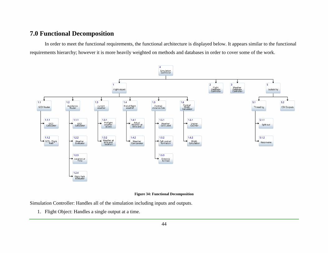
7.0 Functional Decomposition

In order to meet the functional requirements, the functional architecture is displayed below. It appears similar to the functional

requirements hierarchy; however it is more heavily weighted on methods and databases in order to cover some of the work.

Figure 34: Functional Decomposition

Simulation Controller: Handles all of the simulation including inputs and outputs.

1. Flight Object: Handles a single output at a time.

45

2. Flight Database Controller: Interfaces with the flight database in order to gather necessary data.

3. Weather Database Controller: Interfaces with the weather database in order to gather necessary data.

4. Scalability: Handles all of the optimization for the simulation.

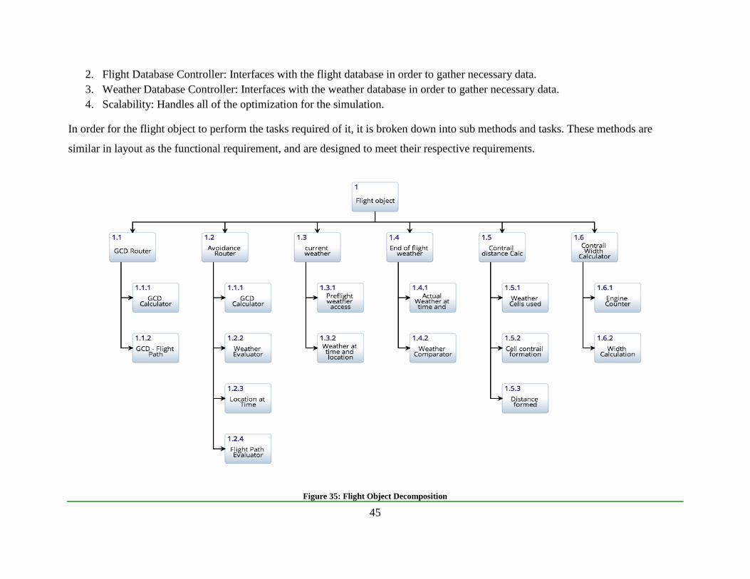
In order for the flight object to perform the tasks required of it, it is broken down into sub methods and tasks. These methods are

similar in layout as the functional requirement, and are designed to meet their respective requirements.

Figure 35: Flight Object Decomposition

46

The following is an outline of descriptions for all the functions represented in the previous

diagram.

1. Flight Object: Handles one flight in order to produce the correct output.

1.1. GCD Router: Routes the aircraft through the great circle path.

1.1.1. GCD Calculator: Calculates the great circle distance and path.

1.1.2. GCD - Flight Path: Converts the distance to a usable flight path.

1.2. Avoidance Router: Routes the aircraft in such a way that avoids contrail formation.

1.2.1. GCD Calculator: Calculates the great circle distance and path.

1.2.2. Weather Evaluator: Evaluates weather cells to determine which are likely to form

contrails.

1.2.3. Location at Time: Determines which location the aircraft would be at for a given

time; based on distance traveled along flight path.

1.2.4. Flight Path Evaluator: Determines the optimal flight path for the aircraft to follow

in order to avoid contrails.

1.3. Current Weather: Gathers the weather data available to the aircraft prior to take off.

1.3.1. Preflight weather access: Accesses the weather database in order to gather the

needed weather data.

1.3.2. Weather Data at Time and Location: Gathers data for a given weather cell at a

given time.

1.4. End of Flight weather: Gathers weather data necessary to determine if contrails formed.

1.4.1. Actual Weather at time and location: Gathers RAP and RUC data for the given

location and time.

1.4.2. Weather Comparator: Compares actual weather data to the predicted weather

data.

1.5. Contrail distance calc: Records the distances of contrails formed.

1.5.1. Weather Cells used: Determines which weather cells were used by an aircraft.

1.5.2. Cell Contrail formation: Determines if an aircraft formed a contrail.

1.5.3. Distance Formed: Determines the miles of contrails a flight formed.

1.6. Contrail width calculator: Calculates the width of contrails formed by an aircraft.

1.6.1. Engine Counter: Determines the number of engines an aircraft has.

1.6.2. Width Calculation: Determines the width of the contrails formed by an aircraft.

47

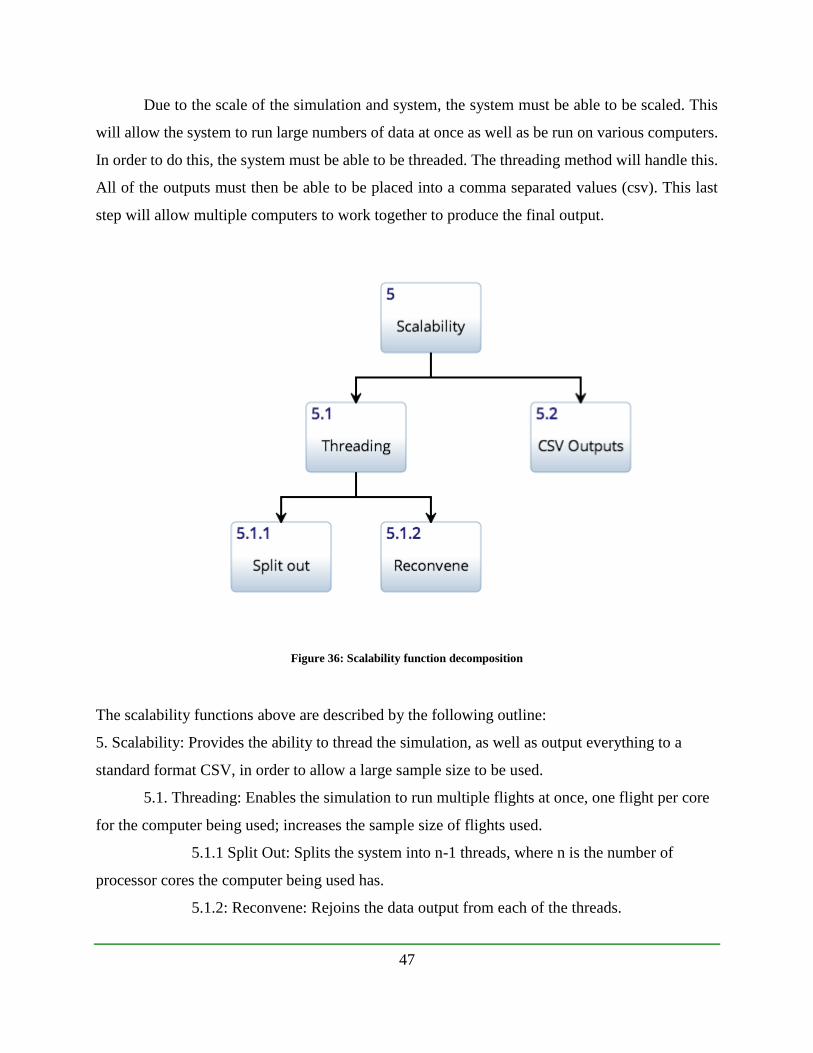
Due to the scale of the simulation and system, the system must be able to be scaled. This

will allow the system to run large numbers of data at once as well as be run on various computers.

In order to do this, the system must be able to be threaded. The threading method will handle this.

All of the outputs must then be able to be placed into a comma separated values (csv). This last

step will allow multiple computers to work together to produce the final output.

Figure 36: Scalability function decomposition

The scalability functions above are described by the following outline:

5. Scalability: Provides the ability to thread the simulation, as well as output everything to a

standard format CSV, in order to allow a large sample size to be used.

5.1. Threading: Enables the simulation to run multiple flights at once, one flight per core

for the computer being used; increases the sample size of flights used.

5.1.1 Split Out: Splits the system into n-1 threads, where n is the number of

processor cores the computer being used has.

5.1.2: Reconvene: Rejoins the data output from each of the threads.

48

5.2: CSV Outputs: Outputs all of the information in order for the system to be able to use

multiple computers at the same time in order to run the simulation, and increase the sample size.

49

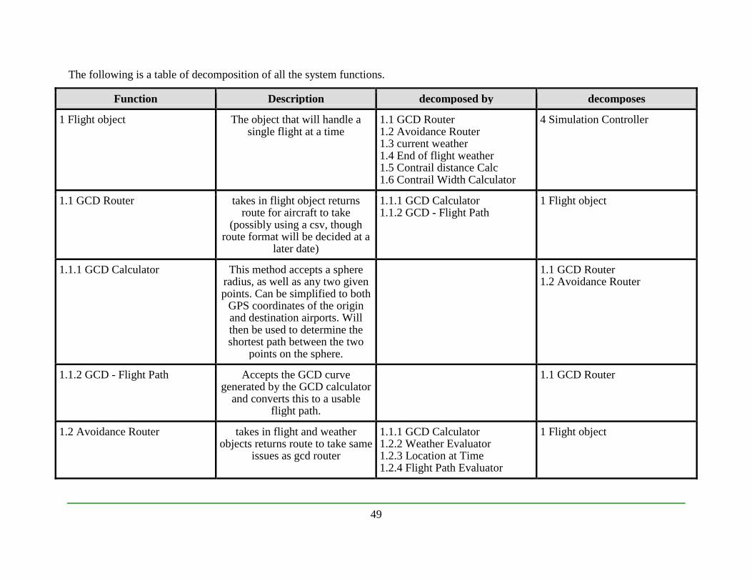
The following is a table of decomposition of all the system functions.

Function Description decomposed by decomposes

1 Flight object The object that will handle a single flight at a time

1.1 GCD Router 1.2 Avoidance Router 1.3 current weather 1.4 End of flight weather 1.5 Contrail distance Calc 1.6 Contrail Width Calculator

4 Simulation Controller

1.1 GCD Router takes in flight object returns route for aircraft to take

(possibly using a csv, though route format will be decided at a

later date)

1.1.1 GCD Calculator 1.1.2 GCD - Flight Path

1 Flight object

1.1.1 GCD Calculator This method accepts a sphere radius, as well as any two given points. Can be simplified to both

GPS coordinates of the origin and destination airports. Will then be used to determine the shortest path between the two

points on the sphere.

1.1 GCD Router 1.2 Avoidance Router

1.1.2 GCD - Flight Path Accepts the GCD curve generated by the GCD calculator

and converts this to a usable flight path.

1.1 GCD Router

1.2 Avoidance Router takes in flight and weather objects returns route to take same

issues as gcd router

1.1.1 GCD Calculator 1.2.2 Weather Evaluator 1.2.3 Location at Time 1.2.4 Flight Path Evaluator

1 Flight object

50

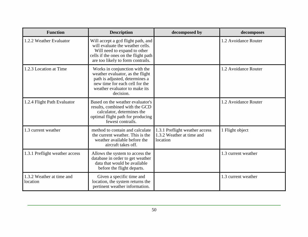
Function Description decomposed by decomposes

1.2.2 Weather Evaluator Will accept a gcd flight path, and will evaluate the weather cells. Will need to expand to other

cells if the ones on the flight path are too likely to form contrails.

1.2 Avoidance Router

1.2.3 Location at Time Works in conjunction with the weather evaluator, as the flight path is adjusted, determines a new time for each cell for the weather evaluator to make its

decision.

1.2 Avoidance Router

1.2.4 Flight Path Evaluator Based on the weather evaluator's results, combined with the GCD

calculator, determines the optimal flight path for producing

fewest contrails.

1.2 Avoidance Router

1.3 current weather method to contain and calculate the current weather. This is the

weather available before the aircraft takes off.

1.3.1 Preflight weather access 1.3.2 Weather at time and location

1 Flight object

1.3.1 Preflight weather access Allows the system to access the database in order to get weather

data that would be available before the flight departs.

1.3 current weather

1.3.2 Weather at time and location

Given a specific time and location, the system returns the pertinent weather information.

1.3 current weather

51

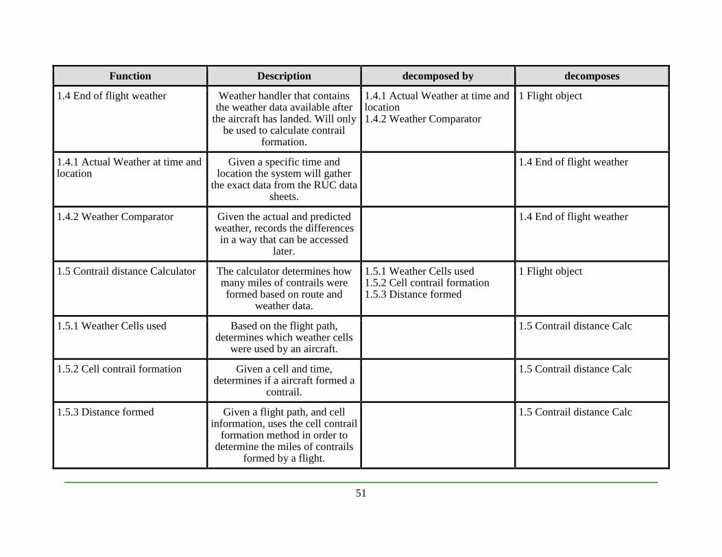
Function Description decomposed by decomposes

1.4 End of flight weather Weather handler that contains the weather data available after

the aircraft has landed. Will only be used to calculate contrail

formation.

1.4.1 Actual Weather at time and location 1.4.2 Weather Comparator

1 Flight object

1.4.1 Actual Weather at time and location

Given a specific time and location the system will gather

the exact data from the RUC data sheets.

1.4 End of flight weather

1.4.2 Weather Comparator Given the actual and predicted weather, records the differences

in a way that can be accessed later.

1.4 End of flight weather

1.5 Contrail distance Calculator The calculator determines how many miles of contrails were formed based on route and

weather data.

1.5.1 Weather Cells used 1.5.2 Cell contrail formation 1.5.3 Distance formed

1 Flight object

1.5.1 Weather Cells used Based on the flight path, determines which weather cells

were used by an aircraft.

1.5 Contrail distance Calc

1.5.2 Cell contrail formation Given a cell and time, determines if a aircraft formed a

contrail.

1.5 Contrail distance Calc

1.5.3 Distance formed Given a flight path, and cell information, uses the cell contrail

formation method in order to determine the miles of contrails

formed by a flight.

1.5 Contrail distance Calc

52

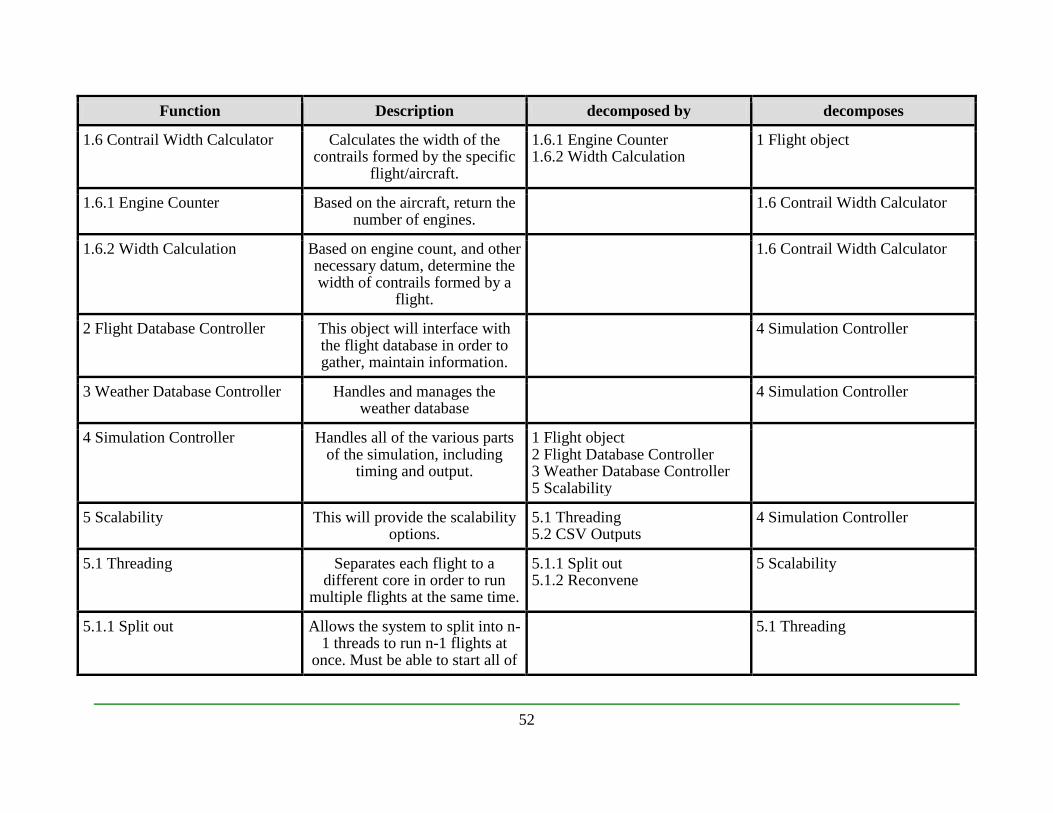
Function Description decomposed by decomposes

1.6 Contrail Width Calculator Calculates the width of the contrails formed by the specific

flight/aircraft.

1.6.1 Engine Counter 1.6.2 Width Calculation

1 Flight object

1.6.1 Engine Counter Based on the aircraft, return the number of engines.

1.6 Contrail Width Calculator

1.6.2 Width Calculation Based on engine count, and other necessary datum, determine the width of contrails formed by a

flight.

1.6 Contrail Width Calculator

2 Flight Database Controller This object will interface with the flight database in order to gather, maintain information.

4 Simulation Controller

3 Weather Database Controller Handles and manages the weather database

4 Simulation Controller

4 Simulation Controller Handles all of the various parts of the simulation, including

timing and output.

1 Flight object 2 Flight Database Controller 3 Weather Database Controller 5 Scalability

5 Scalability This will provide the scalability options.

5.1 Threading 5.2 CSV Outputs

4 Simulation Controller

5.1 Threading Separates each flight to a different core in order to run

multiple flights at the same time.

5.1.1 Split out 5.1.2 Reconvene

5 Scalability

5.1.1 Split out Allows the system to split into n-1 threads to run n-1 flights at

once. Must be able to start all of

5.1 Threading

53

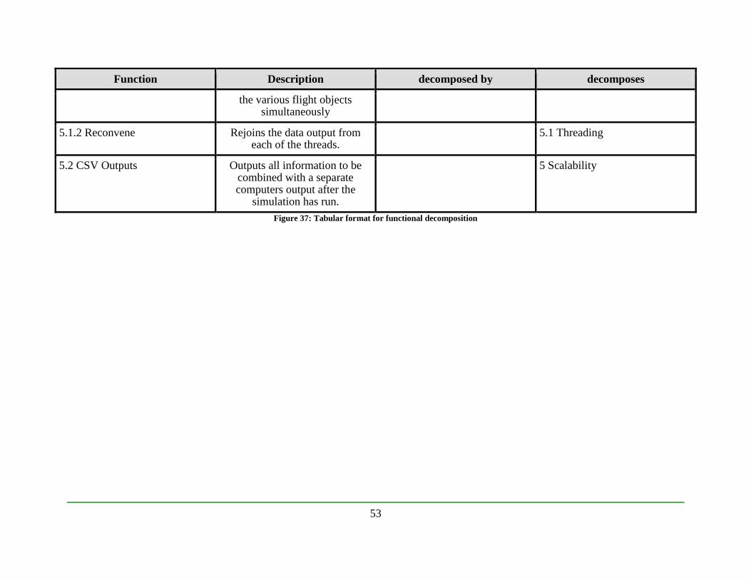
Function Description decomposed by decomposes

the various flight objects simultaneously

5.1.2 Reconvene Rejoins the data output from each of the threads.

5.1 Threading

5.2 CSV Outputs Outputs all information to be combined with a separate computers output after the

simulation has run.

5 Scalability

Figure 37: Tabular format for functional decomposition

54

8.0 Method of Analysis

8.1 Design Alternatives

Flight path adjustment alternatives provide flight paths that avoid regions in which an

aircraft is prone to creating persistent contrails. The goal of the system is to provide a strategic

flight plan for each individual commercial flight. The input of the system is the integration of the

Rapid Update Cycle (RUC) weather system developed by the National Oceanic & Atmospheric

Administration (NOAA) and historical flight paths obtained from the Federal Aviation

Administration (FAA). The flight path computation for the aircraft involves using humidity and

temperature provided by the RUC database to calculate areas with a relative humidity with respect

to ice (RHi) that is greater than or equal to 100% (Bower, 2008). The system will also perform a

tradeoff between creating a flight path, the fuel consumption, as well as the amount of emissions

in the creation of an optimal flight path.

Flight distances have been categorized by Short ( < 500 nm), Medium (500 – 1000 nm),

and Long ( > 1000 nm). Along with these categories, an array of ISSR avoidance aggressiveness

(no avoidance, partial avoidance, total avoidance) was applied to all flights to create different

aggressiveness of ISSR avoidance levels. The no avoidance alternative represents the (GCD), and

the total avoidance alternative represents as much avoidance as possible. The system then

generated a flight path for each flight length and ISSR avoidance aggressiveness.

Combining the contrail avoidance heuristics and the flight distances at which the avoidance

is being attempted results in 9 possible alternatives. The following figure represents the 9 design

alternatives. Note that complete avoidance is only attempted if the origin or destination airport is

not within ISSR.

Design Alternative Avoidance Aggressiveness Flight Length

1 No Avoidance Short

2 No Avoidance Medium

3 No Avoidance Long

55

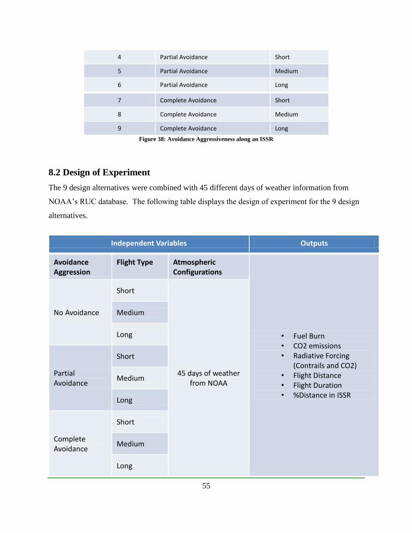
4 Partial Avoidance Short

5 Partial Avoidance Medium

6 Partial Avoidance Long

7 Complete Avoidance Short

8 Complete Avoidance Medium

9 Complete Avoidance Long

Figure 38: Avoidance Aggressiveness along an ISSR

8.2 Design of Experiment

The 9 design alternatives were combined with 45 different days of weather information from

NOAA’s RUC database. The following table displays the design of experiment for the 9 design

alternatives.

Independent Variables Outputs

Avoidance Aggression

Flight Type Atmospheric Configurations

• Fuel Burn

• CO2 emissions • Radiative Forcing

(Contrails and CO2) • Flight Distance

• Flight Duration

• %Distance in ISSR

No Avoidance

Short

45 days of weather from NOAA

Medium

Long

Partial Avoidance

Short

Medium

Long

Complete Avoidance

Short

Medium

Long

56

9.0 Simulation Design

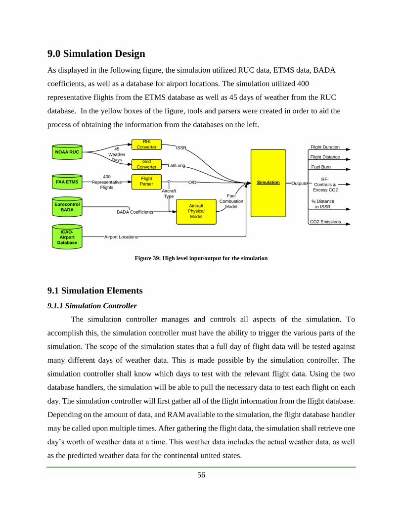
As displayed in the following figure, the simulation utilized RUC data, ETMS data, BADA

coefficients, as well as a database for airport locations. The simulation utilized 400

representative flights from the ETMS database as well as 45 days of weather from the RUC

database. In the yellow boxes of the figure, tools and parsers were created in order to aid the

process of obtaining the information from the databases on the left.

Figure 39: High level input/output for the simulation

9.1 Simulation Elements

9.1.1 Simulation Controller

The simulation controller manages and controls all aspects of the simulation. To

accomplish this, the simulation controller must have the ability to trigger the various parts of the

simulation. The scope of the simulation states that a full day of flight data will be tested against

many different days of weather data. This is made possible by the simulation controller. The

simulation controller shall know which days to test with the relevant flight data. Using the two

database handlers, the simulation will be able to pull the necessary data to test each flight on each

day. The simulation controller will first gather all of the flight information from the flight database.

Depending on the amount of data, and RAM available to the simulation, the flight database handler

may be called upon multiple times. After gathering the flight data, the simulation shall retrieve one

day’s worth of weather data at a time. This weather data includes the actual weather data, as well

as the predicted weather data for the continental united states.

57

The simulation will then create a new flight object for each flight each day. This will create

a very large number of flight objects, and is where the scalability will likely help the most. By

creating a new flight object on open CPU’s, the simulation will be able to run a large number of

flights at once. Once a flight object is finished, the simulation controller shall gather all of the

output data from each flight. This includes flight time, fuel used, and miles of contrails produced.

By combining this information with the information from the other flights using the same routing

methods, the controller is able to generate the total flight time, fuel used, and miles of contrails

formed by each of the alternative routers.

All data used for the simulation will be historic data. This allows for validation of weather

predictions against the actual simulation output. By using the weather data, it can be determined

whether contrails were created when aircraft flew through a certain area of the sky. If the

simulation results match up with historical data, then it will be determined that the system will be

able to correctly avoid forming contrails. In order to control and run the simulation, the controller

will access the flight database, and obtain the “next” flight. It will then use the data from this flight

in order to create a flight object.

58

9.1.2 Flight Object

The flight object will be run many times by the simulation controller. Each instance of the

flight object shall calculate the five different alternate flight routes. Each flight path must then

output the amount of fuel used, flight duration, and miles of contrails formed. This information

will later be combined with the information from other flights that used the same avoidance method

in order to determine totals for each routing method. To do this, the flight object must receive the

flight and weather information. The flight information contains the type of aircraft, origin airport,

destination airport, as well as the time and date of the flight. Based on the type of aircraft, the flight

object shall be able to apply aircraft maneuvering equations such as thrust and drag to determine

how much fuel was used by a certain flight. The fuel used by a flight, however, is not solely

dependent on the type of aircraft, but the weather as well. In order ultimately determine the fuel

costs of each route, the weather data available to the aircraft must be used. By using the weather

data provided by NOAA, and assuming the weather data to be factual, the system is able to

determine how many miles of contrails were formed as well as the amount of fuel and time used

to accomplish the flight.

9.1.3 Flight Database Handler

The flight database handler shall be able to handle the FAA flight database in order to give

the simulation controller a list of flights. The information that will be handed to the controller will

involve the aircraft model, origin airport, destination airport, historically accurate flight path, and

nominal flight information. FAA ETMS Database

A sample of 400 flights on one day was randomly selected from the FAA’s Enhanced

Traffic Management System (ETMS) database. The quantity of flights for this experiment was

constrained by the computational resources available to run the simulation. Additionally, the

sample of 400 flights was subdivided into categories of long, medium, and short distance flights.

Each category contained a representative sample of flights representative of the day of flight data

available to use. Therefore, 39% of the flights were short distance, 20% were medium distance,

and 42% of the flights were long distance.

59

9.1.4 Weather Database Handler

The National Oceanic and Atmospheric Administration (NOAA)’s Rapid Update Cycle

(RUC) database was utilized for this analysis. 45 different days of weather data from NOAA’s

RUC database were used to represent a small sample of atmospheric configurations. The weather

information included Temperature data, Relative Humidity with respect to water, as well as a

multitude of other variables. All of the weather information was encoded into cells of 13.54x13.54

kilometers on a Lambert Conformal Conic map projection. All the data presented in the grid was

in units of kilometers from a reference point; therefore, a tool was created to determine latitude

and longitude values.

9.1.5 Great Circle Distance Router

In order to calculate the shortest route that an aircraft can fly from one airport to another,

the great circle distance is taken into account. In mathematical terms, the great circle distance is

the shortest line that can join any two points on a sphere. Due to the spherical nature of the Earth,

these equations can be applied in order to determine the shortest route between two points

(airports). After computing the shortest curve between the two airports, the system will then be

able to prepare the flight path based off of this route. The process for generating the GCD route is

as follows:

∆𝜎 = arccos(sin𝜑1 sin𝜑2 + cos𝜑1 cos𝜑2 cos ∆𝜆)

where, 𝜑and 𝜆are the latitude and longitude for the airports. ∆𝜆 is the difference in longitude

between the two airports. To calculate the distance between the two airports, and therefore the

route distance, the following equation is used:

𝑑 = 𝑟∆𝜎

where d is the distance and r is the radius of the earth.

9.2 System Inputs

9.2.1 Weather Input

The current weather grid is obtained from NOAA’s Rapid Update Cycle database. Every hour,

NOAA outputs a .grib2 file that can be converted to a csv and then input into the simulation.

60

Specifically, the Relative Humidity with respect to water (RHw) is combined with Temperature

(T) data from the .grib2 file to create another grid with Ice Supersaturated Regions. The following

model, known as the Schmidt-Appleman criterion, represents RHw and T combining as a function

of Relative Humidity with respect to ice (RHi):

(Sridhar, 2011)

If the region will produce a contrail, (RHi > 100%), then the grid is marked with the value of 1. If

the region would not produce a contrail, relative humidity with respect to ice of less than 100%,

then the region is marked with a 0. 2) Aircraft Type (i.e. B737)

9.2.2 Aircraft Information

The type of aircraft flying is gathered from the FAA’s Enhanced Traffic Management System

(ETMS). The type of aircraft and various information specific to the aircraft from the can be input

into aircraft physical models with Eurocontrol’s Base of Aircraft Data (BADA) coefficients to

calculate time in flight, fuel use, and CO2 produced by the aircraft over the course of the flight.

The following model represents aircraft rate of fuel burn where Hp represents the altitude, VTAS

represents true airspeed, and Cx represent BADA coefficients.

(Eurocontrol, 2011) .

Once the fuel consumption is multiplied by time in air, CO2 emissions can be calculated in

kilograms, using the following equation,

(Jardine, 2009)

where f is the fuel in kilograms, and c is a constant equal to 3.175.

9.2.3 Flight Plan Data

Using ETMS tracking data, the origin, destination, and location updates on aircraft can be

𝑓𝑐𝑟 = 𝐶𝑓1 1 +𝑉𝑇𝐴𝑆

𝐶𝑓2 𝐶𝑇𝐶𝑅 ∗ 𝐶𝑇𝐶,1 1 −

𝐻𝑝

𝐶𝑇𝐶,2+ 𝐶𝑇𝐶,3 ∗ 𝐻𝑝

2 𝐶𝑓𝑐𝑟

61

determined. More specifically, for this system, the ETMS data will only be considered for

determining where an aircraft enters into cruising altitude and where it leaves cruising altitude.

Furthermore, the 1-minute updates on location from the ETMS database were used to determine

VTAS and the latitude and longitude information of the aircraft. The 1-minute updates were also

used to determine the flight level at which the aircraft is flying.

9.3 Contrail Avoidance Algorithm

The simulation used a 3-dimensional version of the A* algorithm to determine tradeoffs

between entering ISSR cells in the grid provided by the RUC database and the distance to get to

the destination cell of the aircraft. The following graphics display one instance of the A* algorithm.

Essentially the algorithm uses a greedy heuristic to search the areas around it to determine

the shortest cost to go to each cell. The cost calculation is displayed in the graphic below, and is

denoted as the “F” value. The green cell is where the aircraft currently is located, and the blue cells

represent the open set, or all the areas that the aircraft can go into. The red cell is the destination

cell, and the black cells represent ISSR. Each cell is given a d-value as part of the initialization of

the algorithm. The d-values represent the shortest Manhattan distance from the cell to the

destination cell. In order to provide avoidance aggressiveness, “heuristic” values were specified

to or decreases the penalties of entering each ISSR cell. Higher penalties led to increased

avoidance aggressiveness.

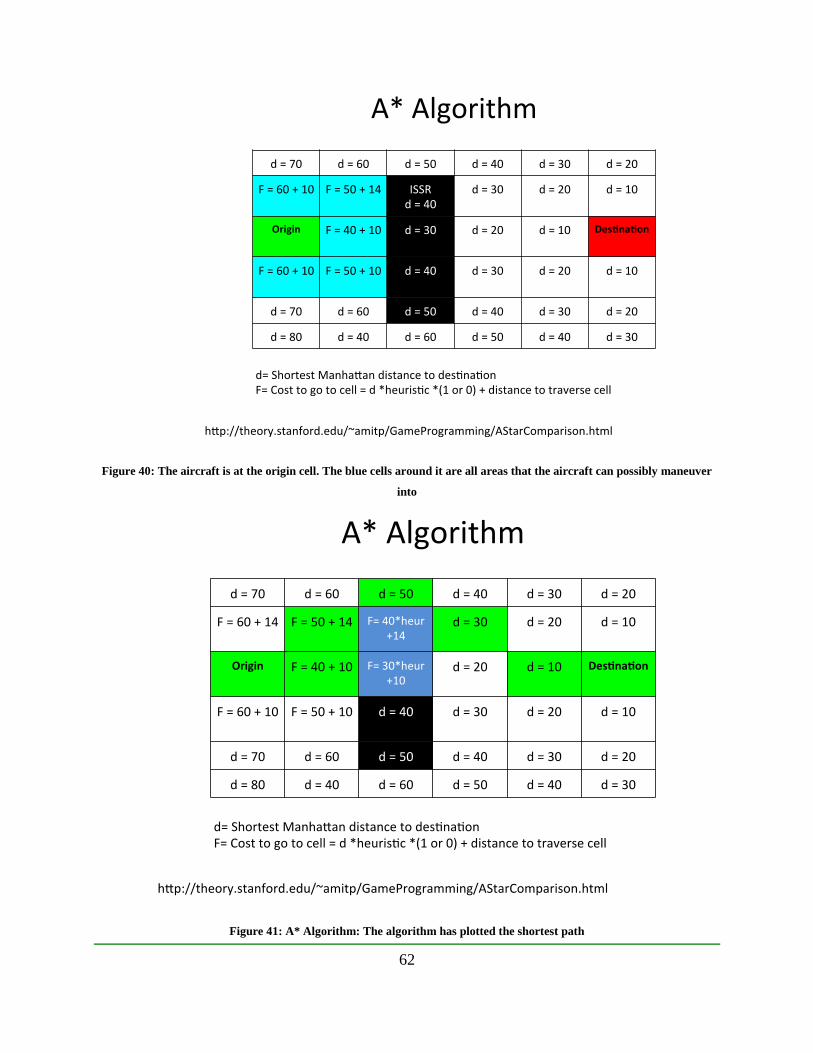
62

Figure 40: The aircraft is at the origin cell. The blue cells around it are all areas that the aircraft can possibly maneuver

into

Figure 41: A* Algorithm: The algorithm has plotted the shortest path

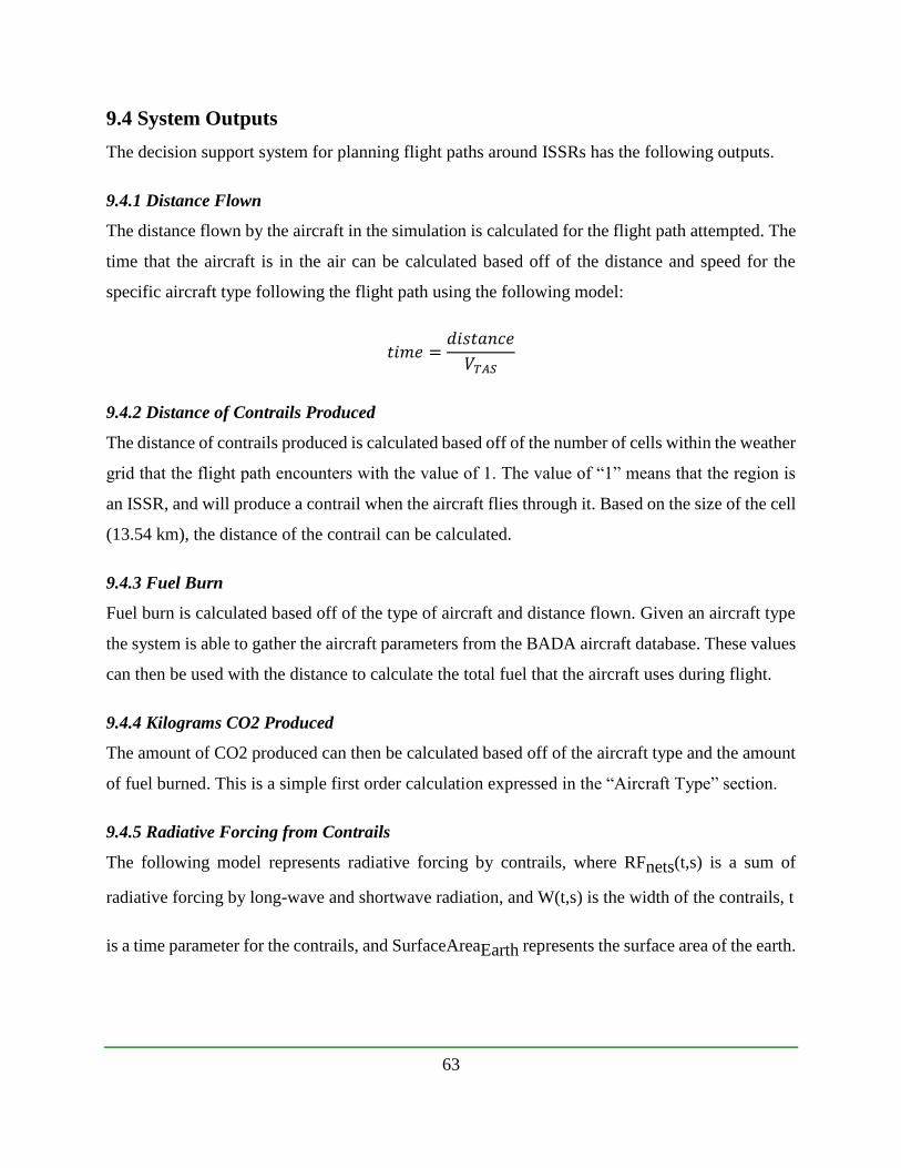
63

9.4 System Outputs

The decision support system for planning flight paths around ISSRs has the following outputs.

9.4.1 Distance Flown

The distance flown by the aircraft in the simulation is calculated for the flight path attempted. The

time that the aircraft is in the air can be calculated based off of the distance and speed for the

specific aircraft type following the flight path using the following model:

𝑡𝑖𝑚𝑒 =𝑑𝑖𝑠𝑡𝑎𝑛𝑐𝑒

𝑉𝑇𝐴𝑆

9.4.2 Distance of Contrails Produced

The distance of contrails produced is calculated based off of the number of cells within the weather

grid that the flight path encounters with the value of 1. The value of “1” means that the region is

an ISSR, and will produce a contrail when the aircraft flies through it. Based on the size of the cell

(13.54 km), the distance of the contrail can be calculated.

9.4.3 Fuel Burn

Fuel burn is calculated based off of the type of aircraft and distance flown. Given an aircraft type

the system is able to gather the aircraft parameters from the BADA aircraft database. These values

can then be used with the distance to calculate the total fuel that the aircraft uses during flight.

9.4.4 Kilograms CO2 Produced

The amount of CO2 produced can then be calculated based off of the aircraft type and the amount

of fuel burned. This is a simple first order calculation expressed in the “Aircraft Type” section.

9.4.5 Radiative Forcing from Contrails

The following model represents radiative forcing by contrails, where RFnets(t,s) is a sum of

radiative forcing by long-wave and shortwave radiation, and W(t,s) is the width of the contrails, t

is a time parameter for the contrails, and SurfaceAreaEarth represents the surface area of the earth.

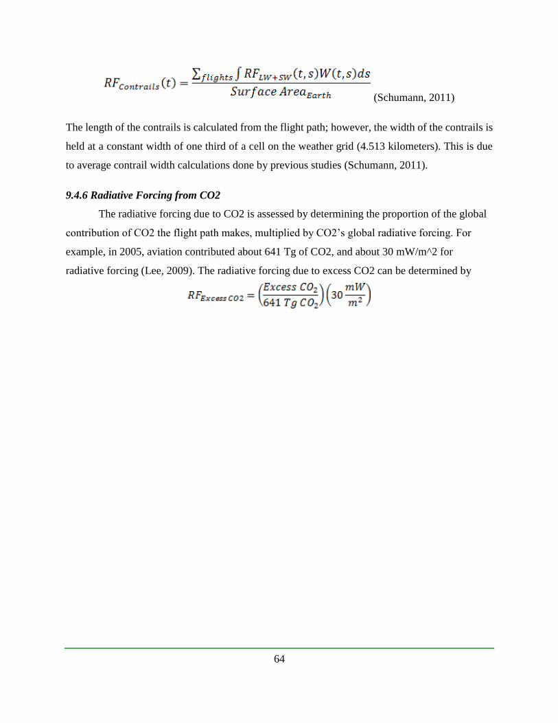
64

(Schumann, 2011)

The length of the contrails is calculated from the flight path; however, the width of the contrails is

held at a constant width of one third of a cell on the weather grid (4.513 kilometers). This is due

to average contrail width calculations done by previous studies (Schumann, 2011).

9.4.6 Radiative Forcing from CO2

The radiative forcing due to CO2 is assessed by determining the proportion of the global

contribution of CO2 the flight path makes, multiplied by CO2’s global radiative forcing. For

example, in 2005, aviation contributed about 641 Tg of CO2, and about 30 mW/m^2 for

radiative forcing (Lee, 2009). The radiative forcing due to excess CO2 can be determined by

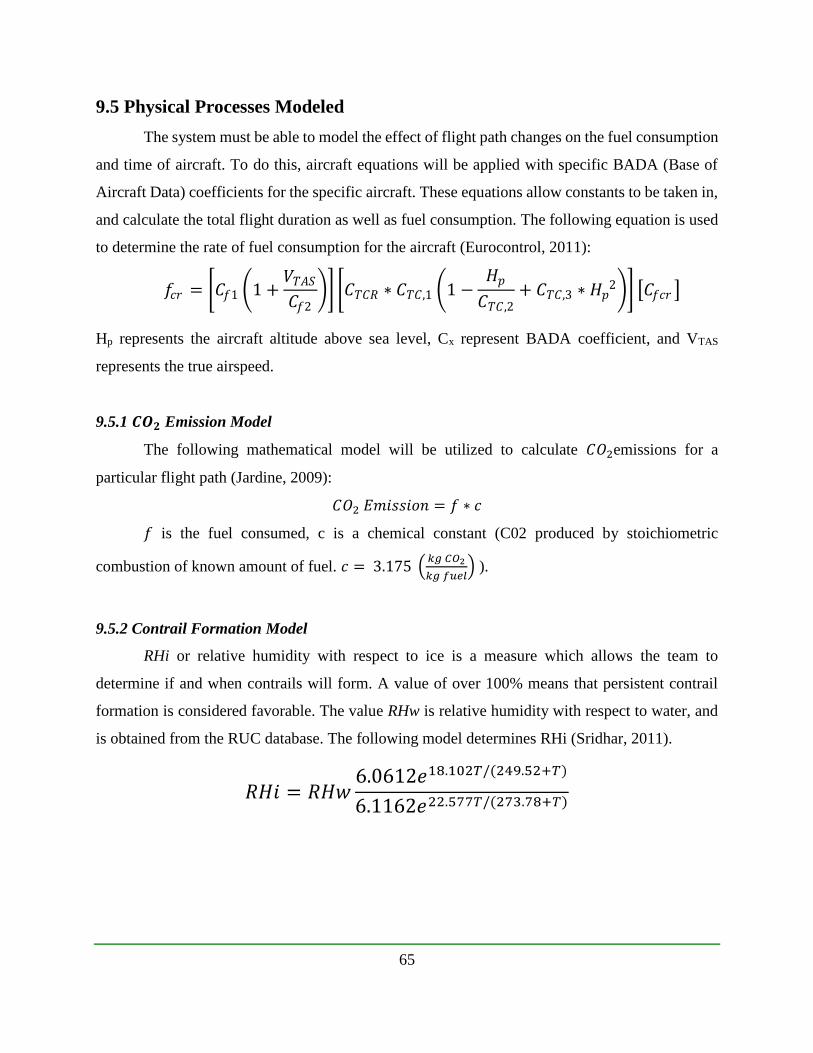
65

9.5 Physical Processes Modeled

The system must be able to model the effect of flight path changes on the fuel consumption

and time of aircraft. To do this, aircraft equations will be applied with specific BADA (Base of

Aircraft Data) coefficients for the specific aircraft. These equations allow constants to be taken in,

and calculate the total flight duration as well as fuel consumption. The following equation is used

to determine the rate of fuel consumption for the aircraft (Eurocontrol, 2011):

Hp represents the aircraft altitude above sea level, Cx represent BADA coefficient, and VTAS

represents the true airspeed.

9.5.1 𝑪𝑶𝟐 Emission Model

The following mathematical model will be utilized to calculate 𝐶𝑂2emissions for a

particular flight path (Jardine, 2009):

𝐶𝑂2𝐸𝑚𝑖𝑠𝑠𝑖𝑜𝑛 = 𝑓 ∗ 𝑐

𝑓 is the fuel consumed, c is a chemical constant (C02 produced by stoichiometric

combustion of known amount of fuel. 𝑐 = 3.175 (𝑘𝑔𝐶𝑂2

𝑘𝑔𝑓𝑢𝑒𝑙) ).

9.5.2 Contrail Formation Model

RHi or relative humidity with respect to ice is a measure which allows the team to

determine if and when contrails will form. A value of over 100% means that persistent contrail

formation is considered favorable. The value RHw is relative humidity with respect to water, and

is obtained from the RUC database. The following model determines RHi (Sridhar, 2011).

𝑓𝑐𝑟 = 𝐶𝑓1 1 +𝑉𝑇𝐴𝑆

𝐶𝑓2 𝐶𝑇𝐶𝑅 ∗ 𝐶𝑇𝐶,1 1 −

𝐻𝑝

𝐶𝑇𝐶,2+ 𝐶𝑇𝐶,3 ∗ 𝐻𝑝

2 𝐶𝑓𝑐𝑟

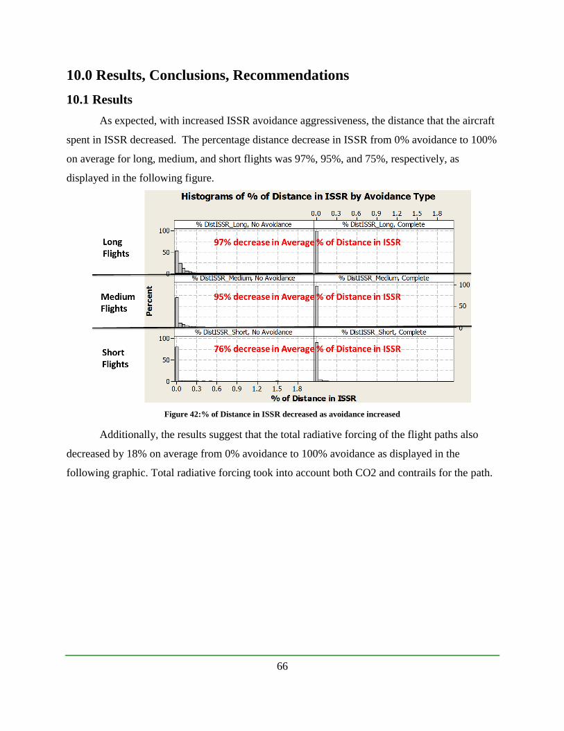
66

10.0 Results, Conclusions, Recommendations

10.1 Results

As expected, with increased ISSR avoidance aggressiveness, the distance that the aircraft

spent in ISSR decreased. The percentage distance decrease in ISSR from 0% avoidance to 100%

on average for long, medium, and short flights was 97%, 95%, and 75%, respectively, as

displayed in the following figure.

Figure 42:% of Distance in ISSR decreased as avoidance increased

Additionally, the results suggest that the total radiative forcing of the flight paths also

decreased by 18% on average from 0% avoidance to 100% avoidance as displayed in the

following graphic. Total radiative forcing took into account both CO2 and contrails for the path.

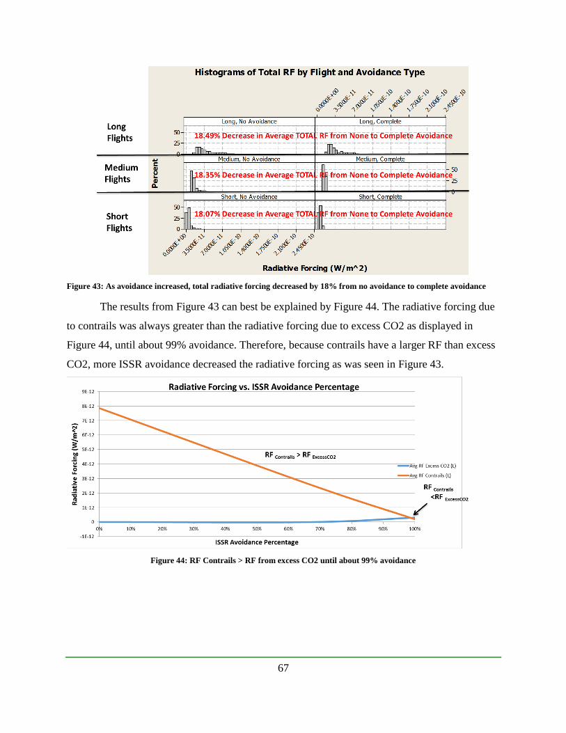
67

Figure 43: As avoidance increased, total radiative forcing decreased by 18% from no avoidance to complete avoidance

The results from Figure 43 can best be explained by Figure 44. The radiative forcing due

to contrails was always greater than the radiative forcing due to excess CO2 as displayed in

Figure 44, until about 99% avoidance. Therefore, because contrails have a larger RF than excess

CO2, more ISSR avoidance decreased the radiative forcing as was seen in Figure 43.

Figure 44: RF Contrails > RF from excess CO2 until about 99% avoidance

68

Similar to Figure 43, Figure 45 displays that the net RF decreased for the flight path as the

avoidance percentage increased. There was about an 18% decrease in RF for each flight type.

Figure 45: About 18% decrease in Total RF as avoidance increases from 0% to 100%

The data also suggested that as the avoidance increased, the cost to avoid ISSR increased,

as was expected. Figure 46 displays a graph for the cost to avoid ISSR for long, medium, and

short flights.

Figure 46: Cost to avoid ISSR increases as ISSR avoidance increases

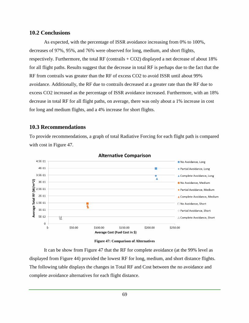
69

10.2 Conclusions

As expected, with the percentage of ISSR avoidance increasing from 0% to 100%,

decreases of 97%, 95%, and 76% were observed for long, medium, and short flights,

respectively. Furthermore, the total RF (contrails + CO2) displayed a net decrease of about 18%

for all flight paths. Results suggest that the decrease in total RF is perhaps due to the fact that the

RF from contrails was greater than the RF of excess CO2 to avoid ISSR until about 99%

avoidance. Additionally, the RF due to contrails decreased at a greater rate than the RF due to

excess CO2 increased as the percentage of ISSR avoidance increased. Furthermore, with an 18%

decrease in total RF for all flight paths, on average, there was only about a 1% increase in cost

for long and medium flights, and a 4% increase for short flights.

10.3 Recommendations

To provide recommendations, a graph of total Radiative Forcing for each flight path is compared

with cost in Figure 47.

Figure 47: Comparison of Alternatives

It can be show from Figure 47 that the RF for complete avoidance (at the 99% level as

displayed from Figure 44) provided the lowest RF for long, medium, and short distance flights.

The following table displays the changes in Total RF and Cost between the no avoidance and

complete avoidance alternatives for each flight distance.

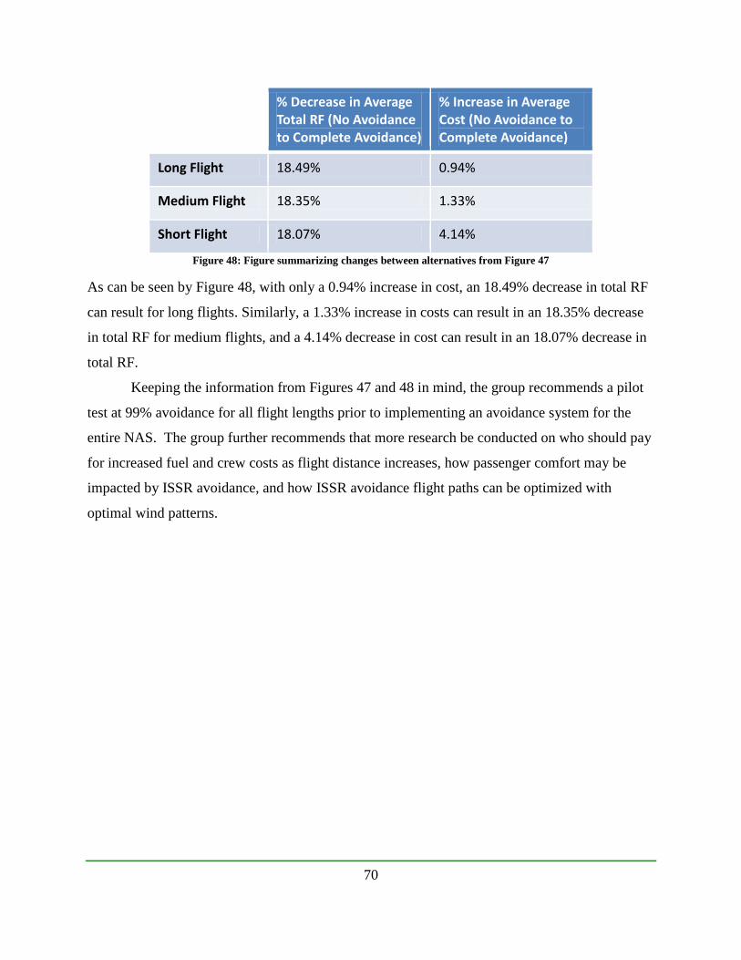
70

% Decrease in Average Total RF (No Avoidance to Complete Avoidance)

% Increase in Average Cost (No Avoidance to Complete Avoidance)

Long Flight 18.49% 0.94%

Medium Flight 18.35% 1.33%

Short Flight 18.07% 4.14%

Figure 48: Figure summarizing changes between alternatives from Figure 47

As can be seen by Figure 48, with only a 0.94% increase in cost, an 18.49% decrease in total RF

can result for long flights. Similarly, a 1.33% increase in costs can result in an 18.35% decrease

in total RF for medium flights, and a 4.14% decrease in cost can result in an 18.07% decrease in

total RF.

Keeping the information from Figures 47 and 48 in mind, the group recommends a pilot

test at 99% avoidance for all flight lengths prior to implementing an avoidance system for the

entire NAS. The group further recommends that more research be conducted on who should pay

for increased fuel and crew costs as flight distance increases, how passenger comfort may be

impacted by ISSR avoidance, and how ISSR avoidance flight paths can be optimized with

optimal wind patterns.

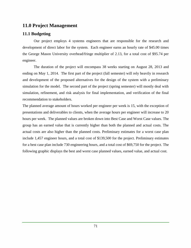
71

11.0 Project Management

11.1 Budgeting

Our project employs 4 systems engineers that are responsible for the research and

development of direct labor for the system. Each engineer earns an hourly rate of $45.00 times

the George Mason University overhead/fringe multiplier of 2.13, for a total cost of $95.74 per

engineer.

The duration of the project will encompass 38 weeks starting on August 28, 2013 and

ending on May 1, 2014. The first part of the project (fall semester) will rely heavily in research

and development of the proposed alternatives for the design of the system with a preliminary

simulation for the model. The second part of the project (spring semester) will mostly deal with

simulation, refinement, and risk analysis for final implementation, and verification of the final

recommendation to stakeholders.

The planned average amount of hours worked per engineer per week is 15, with the exception of

presentations and deliverables to clients, when the average hours per engineer will increase to 20

hours per week. The planned values are broken down into Best Case and Worst Case values. The

group has an earned value that is currently higher than both the planned and actual costs. The

actual costs are also higher than the planned costs. Preliminary estimates for a worst case plan

include 1,457 engineer hours, and a total cost of $139,500 for the project. Preliminary estimates

for a best case plan include 730 engineering hours, and a total cost of $69,750 for the project. The

following graphic displays the best and worst case planned values, earned value, and actual cost.

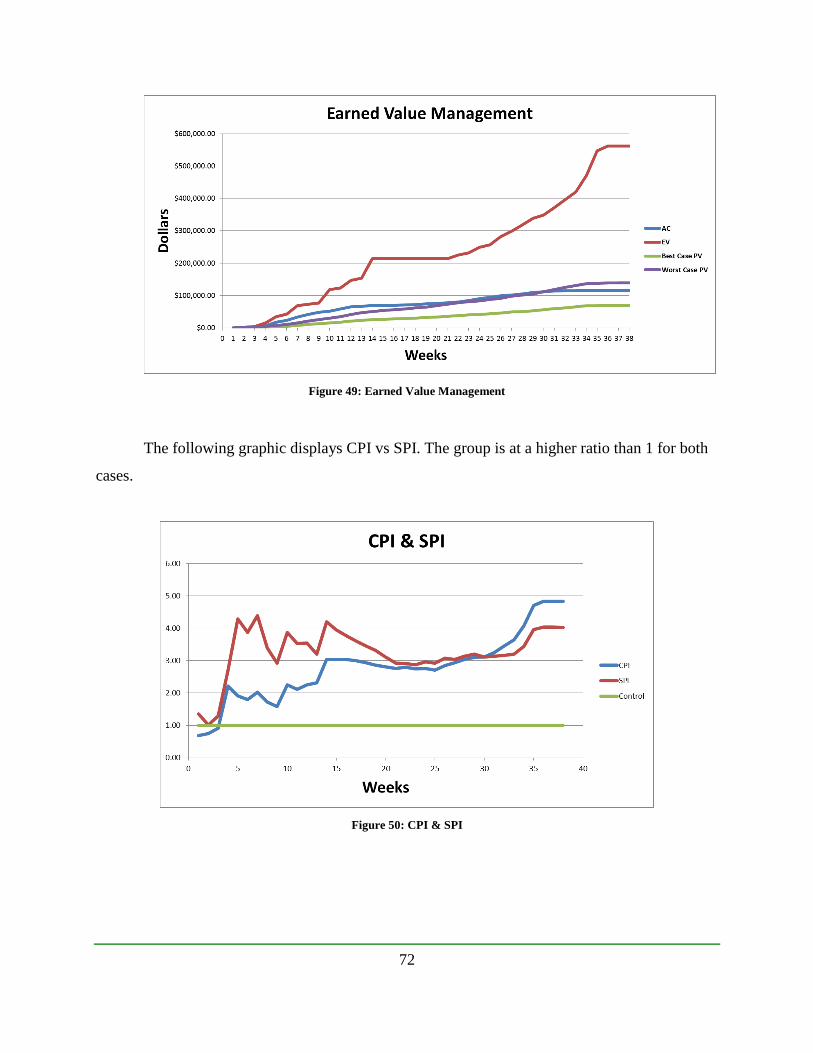
72

Figure 49: Earned Value Management

The following graphic displays CPI vs SPI. The group is at a higher ratio than 1 for both

cases.

Figure 50: CPI & SPI

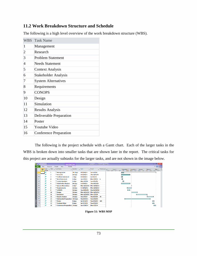
73

11.2 Work Breakdown Structure and Schedule

The following is a high level overview of the work breakdown structure (WBS).

WBS Task Name

1 Management

2 Research

3 Problem Statement

4 Needs Statement

5 Context Analysis

6 Stakeholder Analysis

7 System Alternatives

8 Requirements

9 CONOPS

10 Design

11 Simulation

12 Results Analysis

13 Deliverable Preparation

14 Poster

15 Youtube Video

16 Conference Preparation

The following is the project schedule with a Gantt chart. Each of the larger tasks in the

WBS is broken down into smaller tasks that are shown later in the report. The critical tasks for

this project are actually subtasks for the larger tasks, and are not shown in the image below.

Figure 51: WBS MSP

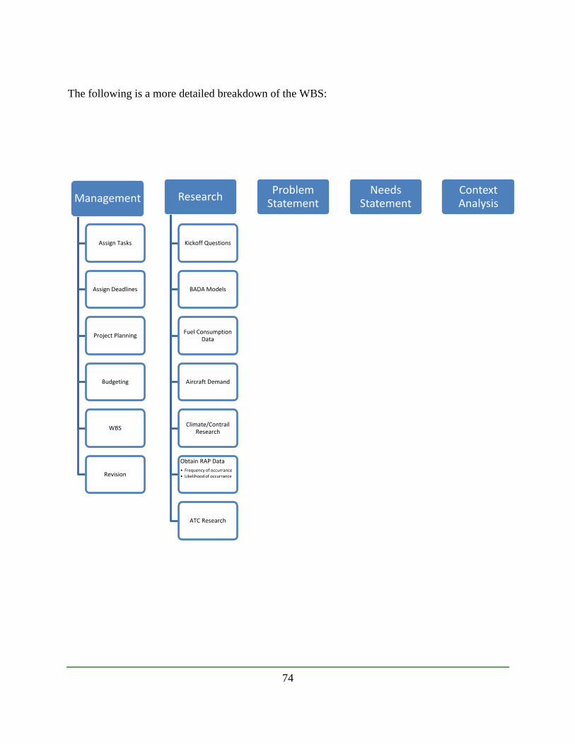
74

The following is a more detailed breakdown of the WBS:

Management

Assign Tasks

Assign Deadlines

Project Planning

Budgeting

WBS

Revision

Research

Kickoff Questions

BADA Models

Fuel Consumption Data

Aircraft Demand

Climate/Contrail Research

Obtain RAP Data

• Frequency of occurrance

• Likelihood of occurrance

ATC Research

Problem Statement

Needs Statement

Context Analysis

75

Stakeholder Analysis

Identify Stakeholders

Win-win situation

System Alternatives

Research high level alternatives

Define flight plan alternatives

Define physical models for alternatives

Conduct weighted analysis

between alternatives

Requirements

Input Requirements

Output Requirements

Functional Requirements

Technology Requirements

CONOPS Design/Modeling

External Systems Design

Functional Hierarchy

Functional Decomposition

76

Simulation

Baseline

Varying Trajectories

Results Analysis

Descriptive Analysis

Inferential Analysis

Results Writeup

Deliverable Preparation

Kickoffs

Prelim Project Plan

Briefing 1 Presentation

Briefing 2 Presentation

Final Project Plan

Briefing 3 Presentation

Faculty Presentation

Proposal Final Report

Proposal Final Presentation

Final Slides

Poster

Proposal Poster

Final Poster

Youtube Video

Conference Prep

Draft of Conference

Paper

Conference Paper

Abstract

77

12.0 References

Airline Fuel Cost and Consumption (U.S. Carriers - Scheduled). (n.d.). (Research and Innovative

Technology Administration) Retrieved from

http://www.transtats.bts.gov/fuel.asp?pn=0&display=data1

Andrew Heymsfield, D. B. (2010). Contrail Microphysics. American Meteorological Society ,

465-472.

Banavar Sridhar, H. N. (2011). Aircraft Trajectory Optimization and Contrails Avoidance in the

Presence of Winds. Journal of Guidance, Control, and Dynamics , 34 (5 ), 1577-1584.

Banavar Sridhar, N. Y. (2013). Energy Efficient Contrail Mitigation Strategies for Reducing the

Environmental Impact of Aviation. 10th USA/Europe Air Traffic Management Research

and Development Semiar (ATM) .

Banavar Sridhar, N. Y. (2010). Fuel Effecient Strategies for Reducing Contrail Formations in

United States Airspace. 29th Digital Avionics Systems Conference .

Bureau of Transportation Statistics (2013). http://www.rita.dot.gov/bts/home

Contrails and Cirrus Clouds from Aviation. (n.d.). (Carbon Offset Research & Education)

Retrieved from http://co2offsetresearch.org/aviation/Contrails.html

EPA United States Environmental Protection Agency. (2013, April ). Retrieved from

http://www.epa.gov/climatechange/ghgemissions/usinventoryreport.html

Federal Aviation Administration. (n.d.). Retrieved September 2013, from

http://aspm.faa.gov/opsnet/sys/Airport.asp

Future Climate Change. (n.d.). (EPA) Retrieved from

http://www.epa.gov/climatechange/science/future.html

Geoffrey C. Bower, I. M. (2008). Multi-objective Aircraft Optimization for Minimum Cost and

Emissions Over Specific Route Networks. 26th international congress of the aeronautical

sciences.

78

Hermann Mannstein, W. K. (2007). Contrail Cirrus Coverage And Radiative Forcing. Proc.

‘Envisat Symposium , 23–27.

Introduction to Greenhouse Gas Emissions from Aviation. (n.d.). (CORE Carbon Offset

Research & Education) Retrieved from

http://co2offsetresearch.org/aviation/AviationImpacts.html

Joyce E. Penner, D. H. (1999). Avaiation And The Blobal Atmosphere. Interngovermental Panel

On Climate Change.

Kevin E. Trenberth, J. T. (2009). Earth's Global Energy Budget. American Meteological Society

, 314.

Lee, D.S. (2009). Aviation and Global Climate Change in the 21st Century. Atmospheric

Environment.

Market-Based Measures. (n.d.). (International Civil Aviation Organization) Retrieved from

http://www.icao.int/environmental-protection/Pages/market-based-measures.aspx

Minnis, P. (2005). Contrails And Cirrus Clouds. NASA Langley Research Center .

Nolan, M. S. Fundamentals of Air Traffic Control, Fifth Edition 2010.

Patrick Minnis, J. K. (2004). Contrails, Cirrus Trends, and Climate. MINNIS ET AL. , 17, 1671-

1684.

Richardson, N. Aviation, Carbon, and the Clean Air Act. Columbia Environmental Law.

Roberto Paoli, J. H. (2004). Contrail formation in aircraft wakes. Journal of Fluid Mechanics,

502, 361-373.

Royal Commission on Environmental Pollution (2002). "The Environmental Effects of Civil

Aviation."

Sassen, K. (1997). Contrail-Cirrus and Their Potential for Regional Climate Change. Bulletin of

the American Meteorological Society , 78 (9), 1885-1903.

79

Schumann, U. (2005). Formation, properties and climatic effects of contrails. Comptes Rendus

Physique, 6 (4), 549-565.

Schumann, U. (2011). “Potential to reduce the climate impact of aviation by flight level

changes.” AIAA Atmospheric Space Environments Conference.

Stoner, J., Wankel, C., & Malleck, S. (2008). Global Sustainability Initiatives: New Models and

New Approaches. Charlotte, N.C.: Information Age Pub..

Tang, S. A. (University of New South Wales). An Assessment of BADA Fuel Flow

Methodologies for In Trail Procedure Evaluation Publication. New South Wales 2010.

The New York Times. (2011, May 3). U.N. Forecasts 10.1 Billion People by Century’s End.

Retrieved October 29, 2013, from

http://www.nytimes.com/2011/05/04/world/04population.html

Travis, D. J. (2004). Regional Variations in U.S. Diurnal Temperature Range for the 11–14

September 2001 Aircraft Groundings: Evidence of Jet Contrail Influence on Climate. J.

Climate , 17 , 1123–1134.

U.S. Air Carrier Traffic Statistics- Domestic Passenger - Revenue Departures Performed (Jan

1996 - Jun 2013). (n.d.). (Research and Innovative Technology Administration) Retrieved

from http://apps.bts.gov/xml/air_traffic/src/datadisp.xml

Ulrike Burkhardt, B. K. (2009). Process-based simulation of contrail cirrus in a global. Journal

Of Geophysical Research, 114, ,doi:10.1029/2008JD011491.