Embed Size (px)
Citation preview
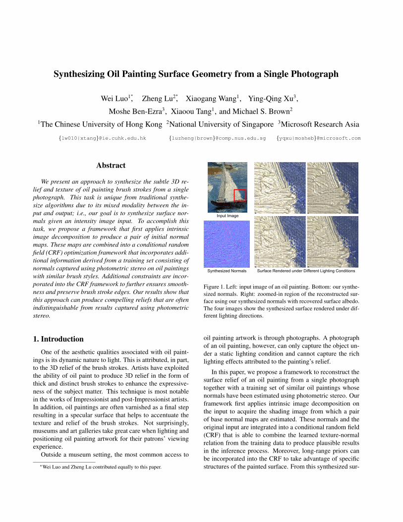
Synthesizing Oil Painting Surface Geometry from a Single Photograph
Wei Luo1∗, Zheng Lu2∗, Xiaogang Wang1, Ying-Qing Xu3,
Moshe Ben-Ezra3, Xiaoou Tang1, and Michael S. Brown2
1The Chinese University of Hong Kong 2National University of Singapore 3Microsoft Research Asia
lw010|[email protected] luzheng|[email protected] yqxu|[email protected]
Abstract
We present an approach to synthesize the subtle 3D re-lief and texture of oil painting brush strokes from a singlephotograph. This task is unique from traditional synthe-size algorithms due to its mixed modality between the in-put and output; i.e., our goal is to synthesize surface nor-mals given an intensity image input. To accomplish thistask, we propose a framework that first applies intrinsicimage decomposition to produce a pair of initial normalmaps. These maps are combined into a conditional randomfield (CRF) optimization framework that incorporates addi-tional information derived from a training set consisting ofnormals captured using photometric stereo on oil paintingswith similar brush styles. Additional constraints are incor-porated into the CRF framework to further ensures smooth-ness and preserve brush stroke edges. Our results show thatthis approach can produce compelling reliefs that are oftenindistinguishable from results captured using photometricstereo.
1. IntroductionOne of the aesthetic qualities associated with oil paint-
ings is its dynamic nature to light. This is attributed, in part,to the 3D relief of the brush strokes. Artists have exploitedthe ability of oil paint to produce 3D relief in the form ofthick and distinct brush strokes to enhance the expressive-ness of the subject matter. This technique is most notablein the works of Impressionist and post-Impressionist artists.In addition, oil paintings are often varnished as a final stepresulting in a specular surface that helps to accentuate thetexture and relief of the brush strokes. Not surprisingly,museums and art galleries take great care when lighting andpositioning oil painting artwork for their patrons’ viewingexperience.
Outside a museum setting, the most common access to
∗Wei Luo and Zheng Lu contributed equally to this paper.
Input Image
Synthesized Normals Surface Rendered under Different Lighting Conditions
Figure 1. Left: input image of an oil painting. Bottom: our synthe-sized normals. Right: zoomed-in region of the reconstructed sur-face using our synthesized normals with recovered surface albedo.The four images show the synthesized surface rendered under dif-ferent lighting directions.
oil painting artwork is through photographs. A photographof an oil painting, however, can only capture the object un-der a static lighting condition and cannot capture the richlighting effects attributed to the painting’s relief.
In this paper, we propose a framework to reconstruct thesurface relief of an oil painting from a single photographtogether with a training set of similar oil paintings whosenormals have been estimated using photometric stereo. Ourframework first applies intrinsic image decomposition onthe input to acquire the shading image from which a pairof base normal maps are estimated. These normals and theoriginal input are integrated into a conditional random field(CRF) that is able to combine the learned texture-normalrelation from the training data to produce plausible resultsin the inference process. Moreover, long-range priors canbe incorporated into the CRF to take advantage of specificstructures of the painted surface. From this synthesized sur-
face normals a 2.5D height field is generated that can pro-duce a visually realistic reconstruction that is hard to distin-guish from that captured by high resolution 3D scans (seeFigure 1).
The remainder of this paper is organized as follows: Sec-tion 2 discusses related work; Section 3 describes the detailsof our framework; Section 4 presents our results. A sum-mary of this work is presented in Section 5.
2. Related WorkWe are unaware of prior work attempting to synthesize
a 2.5D relief of an oil painting from a single photograph,however, several works related to this task are discussed inthe following.
Shape from shading Shape from shading (SfS) [14] isa well-known technique that recovers 3D shapes by usingshading information in an image with known lighting di-rection and surface reflection model. In the case of oilpaintings, directly applying SfS does not produce satis-factory result. This is due to several reasons. First, oneneeds to remove albedo effects before applying SfS byusing techniques such as intrinsic images decomposition[3, 23]. However, a clean separation of shading and re-flectance components is usually hard to obtain [12]. Sec-ond, even with an accurate lighting direction estimation,one intensity value in the image may correspond to differ-ent normals, leading SfS to recover a wrong surface [15].In the case of oil painting surfaces, this one-to-many am-biguity may wrongly recover a convex stroke as a concaveregion. Our method, however, uses an initial normal mapand its mirror reflection estimated from shading as a guid-ance for searching the best-matched normals in the trainingset. This makes our results less sensitive to the mentionedproblems.
Bump mapping and image stylization Bump mappingis a well established technique used to enhance the light-ing effect of a 3D surface by permuting surface normals(e.g., [5, 19]). The map controlling the normal perturba-tion (i.e., the bump map) can be computed using the gradi-ents of an input image that has a distinct texture. This ap-proach typically produces noisy results for oil paintings, asthe content of the painting can be indistinguishable from thestroke relief. Image stylization techniques (e.g., [13, 18])are able to impart artist styles onto input images, videosand renderings of 3D models. These approaches typicallydecompose the input into features that can be parameterizedto guide synthetic brush strokes or particles that simulatebrush strokes. These approaches are not designed to simu-late the 2.5D relief of the strokes themselves. In addition,the input is assumed to be significantly different than thedesired stylized output. Our goal, however, is not to changethe style of the input, but instead to synthesize a 2.5D sur-
face with a similar look and feel.
Imaging relighting, surface modeling, and manipula-tion Other related work involves those targeting image re-lighting (e.g., [6, 28, 27]) and surface modeling and manip-ulation (e.g., [11, 10]) using surface normals. While sharinga commonality of working with normals, these interactiveapproaches would be impractical for specifying individualpaint strokes. As such, our approach performs surface re-construction through surface normal synthesis from train-ing data. Hence, our work is most related to techniques de-signed for constrained texture synthesis (e.g., [7, 20]), andlearning based super resolution (e.g., [8, 24, 22, 25]). Likethese techniques, our approach exploits a training set of ex-emplar patches and uses a learning based method. The maindifference is our focus on synthesizing normals versus pixelvalues.
3. FrameworkThis section briefly describes our oil painting surface
synthesis framework. The overview of the framework andtraining data collection are described first, followed by thedetails of normal synthesis and the surface reconstructionalgorithm. Implementation details are given at the end ofthe section.
3.1. Overview
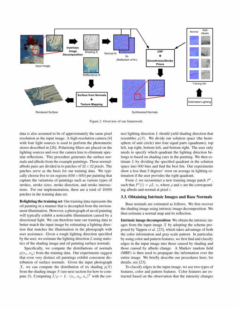
An overview of our framework is shown in Figure 2. Theuser provides an image X which will be used to recover theshading image S and reflection image R through intrinsicimage decomposition. The reflectance R will be used astexture map on the final rendered surface. The shading im-age, S, is used to estimate a pair of initial normal maps,N1 and its reflection N2. We refer to N1, N2 as the basenormals to differentiate from the final synthesized surfacenormals N . In addition, to help tune the training data, ourframework requires the lighting direction of the input im-age, which is estimated from the input image itself with theuser’s help. We then indirectly compute the height field Hby synthesizing the surface normals N . Our normal synthe-sis is a learning based approach exploiting a training set ofexemplar patches whose placement is guided by X , N1 andN2. A CRF is formulated to compute the patch placementonto the output. Through the integration of the synthesizednormals, our method is able to synthesize a convincing 2.5Dgeometry that appears smooth and visually plausible.
3.2. Data Collection
Capture Our training data consists of surface normals andassociated albedos obtained from oil paintings (provided byan art student) that cover the variation of strokes of inputpaintings. Note that the training set is not required to havecomparable aesthetic quality with the input. The training
Input Image
Estimated Lighting
CRF
+Smoothness/Stroke
Priors
Rendered Surface
Shading S
Reflectance R
Relit
AlbedoNormal
Training Set
Instrinsic
Image
Decomposition
Synthesized Normals
Normal N1
N2
(Reflection of N1)
Surface from Normals
+ Texture Mapping
Figure 2. Overview of our framework.
data is also assumed to be of approximately the same pixelresolution as the input image. A high-resolution camera [4]with four light sources is used to perform the photometricstereo described in [26]. Polarizing filters are placed on thelighting sources and over the camera lens to eliminate spec-ular reflections. This procedure generates the surface nor-mals and albedo from the example paintings. These normal-albedo pairs are divided in to patches of 32×32 pixels. Thepatches serve as the basis for our training data. We typi-cally choose five to six regions (600×600) per painting thatcapture the variations of paintings such as various types ofstrokes, stroke sizes, stroke direction, and stroke intersec-tions. For our implementation, there are a total of 48000patches in the training data set.
Relighting the training set Our training data represents theoil painting in a manner that is decoupled from the environ-ment illumination. However, a photograph of an oil paintingwill typically exhibit a noticeable illumination caused by adirectional light. We can therefore tune our training data tobetter match the input image by estimating a lighting direc-tion that matches the illumination in the photograph withuser assistance. Given a rough lighting direction specifiedby the user, we estimate the lighting directionL using statis-tics of the shading image and oil painting surface normals.
Specifically, we compute the distributions of normalsp(nx, ny) from the training data. Our experiments suggestthat even very distinct oil paintings exhibit consistent dis-tribution of surface normals. Given the input photographX , we can compute the distribution of its shading p(S)from the shading image S (see next section for how to com-pute S). Computing I/ρ = L · (nx, ny, nz)T with the cor-
rect lighting direction L should yield shading direction thatresembles p(S). We divide our solution space (the hemi-sphere of unit circle) into four equal parts (quadrants), topleft, top right, bottom left, and bottom right. The user onlyneeds to specify which quadrant the lighting direction be-longs to based on shading cues in the painting. We then es-timate L by dividing the specified quadrant in the solutionspace into 900 bins and find the best bin. Our experimentsshow a less than 5 degrees’ error on average in lighting es-timation if the user provides the right quadrant.
From L we reconstruct a new training image patch P ′ ,such that P ′(i) = ρL ·n, where ρ and n are the correspond-ing albedo and normal at pixel i.
3.3. Obtaining Intrinsic Images and Base Normals
Base normals are estimated as follows. We first recoverthe shading image using intrinsic image decomposition. Wethen estimate a normal map and its reflection.
Intrinsic image decomposition We obtain the intrinsic im-ages from the input image X by adopting the scheme pro-posed by Tappen et al. [23], which takes advantage of boththe color information and gray-scale pattern. In particular,by using color and pattern features, we first find and classifyedges in the input image into those caused by shading andthose caused by albedo change. A Markov random field(MRF) is then used to propagate the information over theentire image. We briefly describe our procedures here; fordetails, see [23].
To classify edges in the input image, we use two types offeatures, color and pattern features. Color features are ex-tracted based on the observation that the intensity changes
due to shading should affect three color channels propor-tionally. Specifically, by normalizing the (R,G,B) tripletat each pixel to unit vector c, we can define the color featureas Fc = arccos (c · c), where c is the average color vectorin neighborhood of c. In our implementation, we use fivescales of neighborhoods sizes, generating five features.
Pattern features are extracted to capture the fact thatshading edges exhibit different shading patterns fromalbedo edges. We define the pattern features as Fg = Ie∗w,where Ie is the patch centered at the edge e, and w is a locallinear filter. In other words, pattern features are extractedby applying a set of linear filters to the neighborhood of anedge. In our implementation, we use Gabor filters with tenorientations and five scales. We found that stroke structuresin the oil painting are well captured using these filters. Intotal, 50 pattern features are generated.
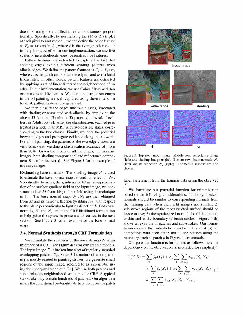
We then classify the edges into two classes, associatedwith shading or associated with albedo, by employing theabove 55 features (5 color + 50 patterns) as weak classi-fiers in AdaBoost [9]. After the classification, each edge istreated as a node in an MRF with two possible states, corre-sponding to the two classes. Finally, we learn the potentialbetween edges and propagate evidence along the network.For an oil painting, the patterns of the two edge classes arevery consistent, yielding a classification accuracy of morethan 90%. Given the labels of all the edges, the intrinsicimages, both shading component S and reflectance compo-nent R can be recovered. See Figure 3 for an example ofintrinsic images.
Estimating base normals The shading image S is usedto estimate the base normal map N1 and its reflection N2.Specifically, by using the gradients of tS as an approxima-tion of he surface gradient field of the input image, we con-struct surfaceM from this gradient field using the techniquein [1]. The base normal maps N1, N2 are then obtainedfrom M and its mirror reflection (yeilding N2) with respectto the plane perpendicular to lighting direction L. Both basenormals, N1 and N2, are in the CRF likelihood formulationto help guide the synthesis process as discussed in the nextsection. See Figure 3 for an example of the base normalmaps.
3.4. Normal Synthesis through CRF Formulation
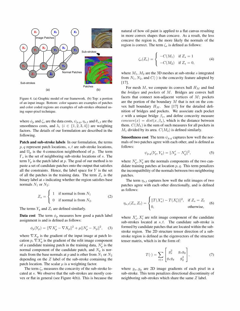
We formulate the synthesis of the normals map N as aninference of a CRF (see Figure 4(a) for our graphic model).The input imageX is broken into a set of regularly sampledoverlapping patches Xp. Since 3D structure of an oil paint-ing is mostly related to painting strokes, we generate smallregions of the input image, referred to as sub-stroke, us-ing the superpixel technique [21]. We use both patches andsub-strokes as neighborhood structures for CRF. A typicalsub-stroke may contain hundreds of patches. Our algorithminfers the conditional probability distribution over the patch
Input Image
Reflectance Shading
N1 N2
Figure 3. Top row: input image. Middle row: reflectance image(left) and shading image (right). Bottom row: base normals N1
(left) and its reflection N2 (right). Zoomed-in regions are alsoshown.
label assignment from the training data given the observedX .
We formulate our potential function for minimizationbased on the following considerations: 1) the synthesizednormals should be similar to corresponding normals fromthe training data when their relit images are similar; 2)sub-stroke regions of the reconstructed surface should beless concave; 3) the synthesized normal should be smoothwithin and at the boundary of brush strokes. Figure 4 (b)shows an example of patches and sub-strokes. Our formu-lation ensures that sub-stroke a and b in Figure 4 (b) arecompatible with each other and all the patches along theboundary, such as patch p in Figure 4, are smooth.
Our potential function is formulated as follows (note thedependency on the observationX is omitted for simplicity):
Ψ(Y, Z) =∑p
φp(Yp) + λ1
∑p
∑q∈Ωp
ψp,q(Yp, Yq)
+ λ2
∑s
ζs(Zs) + λ3
∑s
∑t∈Γs
ηs,t(Zs, Zt)
+ λ4
∑s
∑t∈Γs
θs,t(Zs, Zt, Ys,t),
(1)
Sub-strokes
Patches
pab
(a) (b)
Y2 Y3
Y4 Y6
Y1
X2 X3
X4 X5 X6
X1
Z1
Sub-strokes
Normal Patches
Image Patches
Figure 4. (a) Graphic model of our framework. (b) Top: a portionof an input image. Bottom: color squares are examples of patchesand color coded regions are examples of sub-strokes obtained us-ing super-pixel technique.
where φp and ζs are the data costs, ψp,q , ηs,t and θs,t are thesmoothness costs, and λi (i ∈ 1, 2, 3, 4) are weightingfactors. The details of our formulation are described in thefollowing.
Patch and sub-stroke labels In our formulation, the termsp, q represent patch locations, s, t are sub-stroke locations,and Ωp is the 4-connection neighborhood of p. The termΓs is the set of neighboring sub-stroke locations of s. Theterm Yp is the patch label at p. The goal of our method is topaste a set of candidate patches onto the output that satisfiesall the constraints. Hence, the label space for Y is the setof all the patches in the training data. The term Zs is thebinary label at s indicating whether the region satisfies basenormals N1 or N2:
Zs =
1 if normal is from N1
0 if normal is from N2.(2)
The terms Yq and Zt are defined similarly.
Data cost The term φp measures how good a patch labelassignment is and is defined as follows:
φp(Yp) = ‖∇X ′p −∇Xp‖2 + µ‖N ′
p −Np‖2, (3)
where ∇Xp is the gradient of the input image at patch lo-cation p, ∇X ′
p is the gradient of the relit image componentof a candidate training patch in the training data, N ′
p is thenormal component of the candidate patch, and Np is nor-mals from the base normals at p and is ether from N1 or N2
depending on the Z label of the sub-stroke containing thepatch location. The scalar µ is a weighting factor.
The term ζs measures the concavity of the sub-stroke lo-cated at s. We observe that the sub-strokes are mostly con-vex or flat in general (see Figure 4(b)). This is because the
natural of how oil paint is applied to a flat canvas resultingin more convex shapes than concave. As a result, the lessconcave the region is, the more likely the normals of theregion is correct. The term ζs is defined as follows:
ζs(Zs) =
−C(M1) if Zs = 1
−C(M2) if Zs = 0,(4)
where M1,M2 are the 3D meshes at sub-stroke s integratedfrom N1, N2, and C(·) is the concavity feature adopted by[17].
For mesh M , we compute its convex hull HM and findthe bridges and pockets of M . Bridges are convex hullfacets that connect non-adjacent vertices of M ; pocketsare the portion of the boundary M that is not on the con-vex hull boundary HM . See [17] for the detailed defi-nition of bridges and pockets. We associate each pocketx with a unique bridge βx, and define concavity measureconcave(x) = dist(x, βx), which is the distance betweenthem. C(M1) is the sum of such measures for all pockets inM1 divided by its area. C(M2) is defined similarly.
Smoothness cost The term ψp,q captures how well the nor-mals of two patches agree with each other, and is defined asfollows:
ψp,q(Yp, Yq) = ‖N ′p −N ′
q‖2, (5)
where N ′p, N
′q are the normals components of the two can-
didate training patches at location p, q. This term penalizesthe incompatibility of the normals between two neighboringpatches.
The term ηs,t captures how well the relit images of twopatches agree with each other directionally, and is definedas follows:
ηs,t(Zs, Zt) =
‖T (X ′s)− T (X ′
t)‖2, if Zs = Zt
0, otherwise,(6)
where X ′s, X
′t are relit image component of the candidate
sub-strokes located at s, t. The candidate sub-stroke isformed by candidate patches that are located within the sub-stroke region. The 2D structure tensor direction of a sub-stroke region is defined as the eigenvectors of the structuretenser matrix, which is in the form of:
T (·) =∑i∈s
g2x gxgy
gxgy g2y
, (7)
where gx, gy are 2D image gradients of each pixel in asub-stroke. This term penalizes directional discontinuity ofneighboring sub-strokes which share the same Z label.
Algorithm 1 Minimizing potential Ψ
Initialization: set all Z label to 0. For each patch p, set Yp to thepatch in the training data returned by 1 Nearest Neighbor searchusing Np.Till convergence:
1. Minimize
Ψ1(Y | Z) =∑p
φp + λ1
∑p
∑q∈Ωp
ψp,q
+ λ4
∑s
∑t∈Γs
θs,t,
conditioned on X and Z using Loopy Belief Propagation.
2. Minimize
Ψ2(Z | Y ) = λ2
∑s
ζs + λ3
∑s
∑t∈Γs
ηs,t
+ λ4
∑s
∑t∈Γs
θs,t,
conditioned on X and Y using Loopy Belief Propagation.
Return: Labels Yp. A best cut (see Section 3.5) at each overlap-ping region is found between patches to ensure smoothness.
The term θs,t captures how well the normals of two sub-strokes agree with each other, and is defined as follows:
Dp = min (‖N ′p −N1p‖2, ‖N ′
p −N2p‖2) (8)
θs,t(Zs, Zt, Ys,t) =
∑
p∈Ys,tDp, if Zs 6= Zt
0, otherwise,(9)
where Ys,t is the collection of patches that belong to bothsub-stroke s and t, andN1p,N2p are two base normals at p.This term is used to smooth normals between neighboringsub-strokes. The idea is that the patches at the sub-strokeboundaries should share the same Z label and should besimilar to N1 or N2.
Optimization To minimize our potential function shownin Equation 1, we find the label assignments for patchesand sub-strokes by alternatively minimizing the two poten-tial functions using Loopy Belief Propagation [29], as statedin Algorithm 1. Typically in our experiments, convergenceis obtained after 3 to 4 iterations.
3.5. Implementation Details
We use K nearest neighbor search (KNN) to find patchcandidates in the training data where K is chosen to be 40.We employ PatchMatch [2] to speed up the KNN search,since in our case, both the input image and the training setcontain densely sampled patches. As a result, each KNNsearch takes 0.02s on our training set. For a 2000 × 2000image, it takes 15 minutes in searching and 5 minutes in
inference. Graphcut [16] is used to find the best cut in theoverlapping region between neighboring patches. However,in our case, we use normals instead of using intensity orcolors. As the last step of our framework, the height field isreconstructed from the synthesized normals using the tech-nique presented in [27].
4. ResultsResults from our framework are shown in Figure 5, Fig-
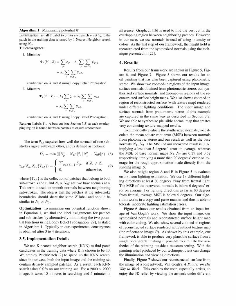
ure 6, and Figure 7. Figure 5 shows our results for anoil painting that has also been captured using photometricstereo. We show two zoomed-in regions of the input image,surface normals obtained from photometric stereo, our syn-thesized surface normals, and zoomed-in regions of the re-constructed surface height maps. We also show a zoomed-inregion of reconstructed surface (with texture map) renderedunder different lighting conditions. The input image andsurface normals from photometric stereo of this exampleare captured in the same way as described in Section 3.2.We are able to synthesize plausible normal map that createsvery convincing texture-mapped results.
To numerically evaluate the synthesized normals, we cal-culate the mean square root error (MSE) between normalsfrom photometric stereo and our result as well as the basenormals N1, N2. The MSE of our recovered result is 0.07,implying a less than 5 degrees’ error on average, whereasthe MSE of base normal maps N1, N2 are 0.37 and 0.52respectively, implying a more than 20 degrees’ error on av-erage for the rough approximation made directly from theshading image S.
We also relight region A and B in Figure 5 to evaluateerrors from lighting estimation. We use 18 different light-ing directions at least 30 degrees away from frontal light.The MSE of the recovered normals is below 6 degrees’ er-ror on average. For lighting directions as far as 60 degreesfrom frontal, average MSE is below 9 degrees. Our algo-rithm works in a copy-and-paste manner and thus is able totolerate moderate lighting estimation errors.
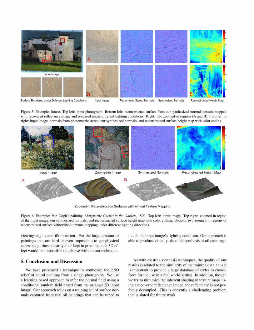
Figure 6 shows our results obtained from an input im-age of Van Gogh’s work. We show the input image, oursynthesized normals and reconstructed surface height mapwith color coding. We also show several zoomed-in regionsof reconstructed surface rendered with/without texture map(the reflectance image R). As shown by this example, ourframework is able to produce very plausible surface from asingle photograph, making it possible to simulate the aes-thetics of the painting outside a museum setting. With thepainting relief produced by our technique, users can changethe illumination and viewing directions.
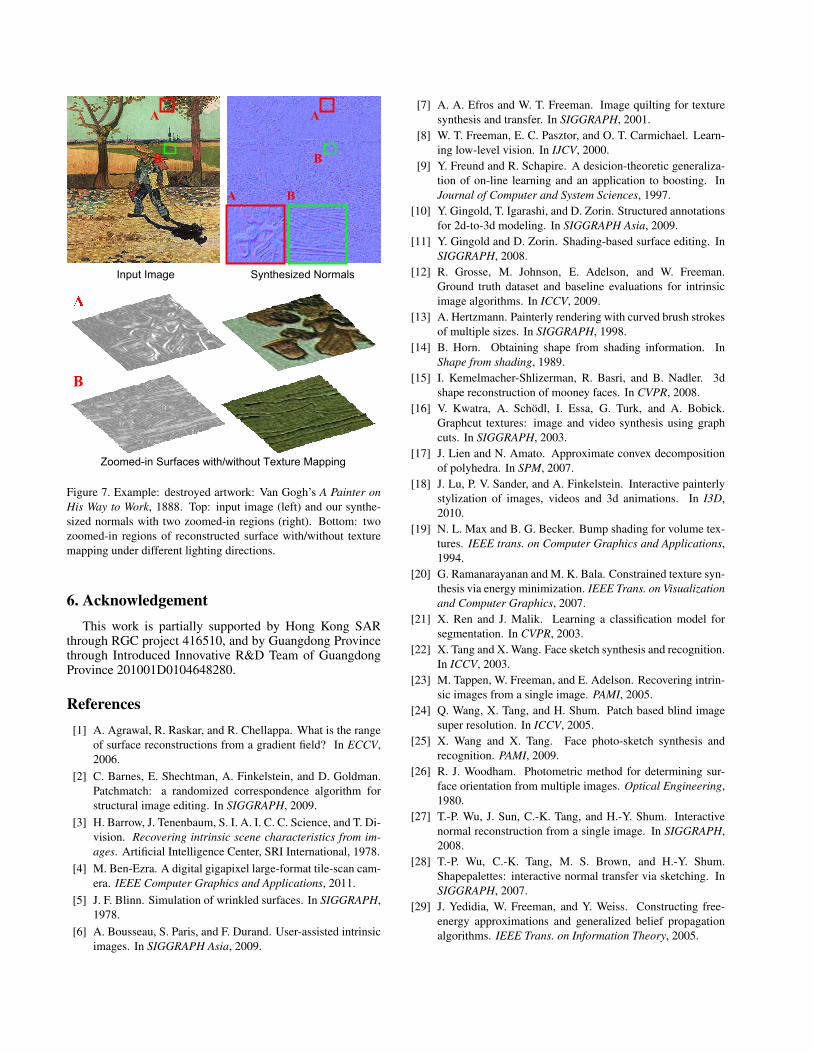
Finally, Figure 7 shows our reconstructed surface fromthe image of a lost artwork, Van Gogh’s A Painter on HisWay to Work. This enables the user, especially artists, toenjoy the 3D relief by viewing the artwork under different
B
A
A
B
25
10
15
20
5
20
15
10
25
5
Input Image
Surface Rendered under Different Lighting Conditions Input Image Photometric Stereo Normals Synthesized Normals Reconstructed Height Map
Figure 5. Example: house. Top left: input photograph. Bottom left: reconstructed surface from our synthesized normals texture mappedwith recovered reflectance image and rendered under different lighting conditions. Right: two zoomed-in regions (A and B), from left toright: input image, normals from photometric stereo, our synthesized normals, and reconstructed surface height map with color coding.
A
B
A B
2
4
66
8
10
12
Input Image Zoomed-in Image Synthesized Normals Reconstructed Height Map
Zoomed-in Reconstruction Surfaces with/without Texture Mapping
Figure 6. Example: Van Gogh’s painting, Marguerite Gachet in the Garden, 1890. Top left: input image. Top right: zoomed-in regionof the input image, our synthesized normals, and reconstructed surface height map with color coding. Bottom: two zoomed-in regions ofreconstructed surface with/without texture mapping under different lighting directions.
viewing angles and illumination. For the large amount ofpaintings that are hard or even impossible to get physicalaccess (e.g., those destroyed or kept in private), such 3D ef-fect would be impossible to achieve without our technique.
5. Conclusion and Discussion
We have presented a technique to synthesize the 2.5Drelief of an oil painting from a single photograph. We usea learning based approach to infer the normal field using aconditional random field based from the original 2D inputimage. Our approach relies on a training set of surface nor-mals captured from real oil paintings that can be tuned to
match the input image’s lighting condition. Our approach isable to produce visually plausible synthesis of oil paintings.
As with existing synthesis techniques, the quality of ourresults is related to the similarity of the training data, thus itis important to provide a large database of styles to choosefrom for the use in a real world setting. In addition, thoughwe try to minimize the inherent shading in texture maps us-ing a recovered reflectance image, the reflectance is not per-fectly decoupled. This is currently a challenging problemthat is slated for future work.
A
B
A
B
A
B
A B
Input Image Synthesized Normals
Zoomed-in Surfaces with/without Texture Mapping
Figure 7. Example: destroyed artwork: Van Gogh’s A Painter onHis Way to Work, 1888. Top: input image (left) and our synthe-sized normals with two zoomed-in regions (right). Bottom: twozoomed-in regions of reconstructed surface with/without texturemapping under different lighting directions.
6. AcknowledgementThis work is partially supported by Hong Kong SAR
through RGC project 416510, and by Guangdong Provincethrough Introduced Innovative R&D Team of GuangdongProvince 201001D0104648280.
References[1] A. Agrawal, R. Raskar, and R. Chellappa. What is the range
of surface reconstructions from a gradient field? In ECCV,2006.
[2] C. Barnes, E. Shechtman, A. Finkelstein, and D. Goldman.Patchmatch: a randomized correspondence algorithm forstructural image editing. In SIGGRAPH, 2009.
[3] H. Barrow, J. Tenenbaum, S. I. A. I. C. C. Science, and T. Di-vision. Recovering intrinsic scene characteristics from im-ages. Artificial Intelligence Center, SRI International, 1978.
[4] M. Ben-Ezra. A digital gigapixel large-format tile-scan cam-era. IEEE Computer Graphics and Applications, 2011.
[5] J. F. Blinn. Simulation of wrinkled surfaces. In SIGGRAPH,1978.
[6] A. Bousseau, S. Paris, and F. Durand. User-assisted intrinsicimages. In SIGGRAPH Asia, 2009.
[7] A. A. Efros and W. T. Freeman. Image quilting for texturesynthesis and transfer. In SIGGRAPH, 2001.
[8] W. T. Freeman, E. C. Pasztor, and O. T. Carmichael. Learn-ing low-level vision. In IJCV, 2000.
[9] Y. Freund and R. Schapire. A desicion-theoretic generaliza-tion of on-line learning and an application to boosting. InJournal of Computer and System Sciences, 1997.
[10] Y. Gingold, T. Igarashi, and D. Zorin. Structured annotationsfor 2d-to-3d modeling. In SIGGRAPH Asia, 2009.
[11] Y. Gingold and D. Zorin. Shading-based surface editing. InSIGGRAPH, 2008.
[12] R. Grosse, M. Johnson, E. Adelson, and W. Freeman.Ground truth dataset and baseline evaluations for intrinsicimage algorithms. In ICCV, 2009.
[13] A. Hertzmann. Painterly rendering with curved brush strokesof multiple sizes. In SIGGRAPH, 1998.
[14] B. Horn. Obtaining shape from shading information. InShape from shading, 1989.
[15] I. Kemelmacher-Shlizerman, R. Basri, and B. Nadler. 3dshape reconstruction of mooney faces. In CVPR, 2008.
[16] V. Kwatra, A. Schodl, I. Essa, G. Turk, and A. Bobick.Graphcut textures: image and video synthesis using graphcuts. In SIGGRAPH, 2003.
[17] J. Lien and N. Amato. Approximate convex decompositionof polyhedra. In SPM, 2007.
[18] J. Lu, P. V. Sander, and A. Finkelstein. Interactive painterlystylization of images, videos and 3d animations. In I3D,2010.
[19] N. L. Max and B. G. Becker. Bump shading for volume tex-tures. IEEE trans. on Computer Graphics and Applications,1994.
[20] G. Ramanarayanan and M. K. Bala. Constrained texture syn-thesis via energy minimization. IEEE Trans. on Visualizationand Computer Graphics, 2007.
[21] X. Ren and J. Malik. Learning a classification model forsegmentation. In CVPR, 2003.
[22] X. Tang and X. Wang. Face sketch synthesis and recognition.In ICCV, 2003.
[23] M. Tappen, W. Freeman, and E. Adelson. Recovering intrin-sic images from a single image. PAMI, 2005.
[24] Q. Wang, X. Tang, and H. Shum. Patch based blind imagesuper resolution. In ICCV, 2005.
[25] X. Wang and X. Tang. Face photo-sketch synthesis andrecognition. PAMI, 2009.
[26] R. J. Woodham. Photometric method for determining sur-face orientation from multiple images. Optical Engineering,1980.
[27] T.-P. Wu, J. Sun, C.-K. Tang, and H.-Y. Shum. Interactivenormal reconstruction from a single image. In SIGGRAPH,2008.
[28] T.-P. Wu, C.-K. Tang, M. S. Brown, and H.-Y. Shum.Shapepalettes: interactive normal transfer via sketching. InSIGGRAPH, 2007.
[29] J. Yedidia, W. Freeman, and Y. Weiss. Constructing free-energy approximations and generalized belief propagationalgorithms. IEEE Trans. on Information Theory, 2005.