SYNTHESIS OF DIFFERENCE PATTERNS FOR MONOPULSE ANTENNAS ... · SYNTHESIS OF DIFFERENCE PATTERNS FOR MONOPULSE ANTENNAS WITH OPTIMAL COMBINA- ... antenna array by observing the shape

Progress In Electromagnetics Research B, Vol. 21, 257–280, 2010

SYNTHESIS OF DIFFERENCE PATTERNS FORMONOPULSE ANTENNAS WITH OPTIMAL COMBINA-TION OF ARRAY-SIZE AND NUMBER OF SUBARRAYS— A MULTI-OBJECTIVE OPTIMIZATION APPROACH

S. Pal, S. Das, and A. Basak

Department of Electronics and Telecommunication EngineeringJadavpur UniversityKolkata 700032, India

P. N. Suganthan

School of Electrical and Electronic EngineeringNanyang Technological UniversitySingapore 639798, Singapore

Abstract—Monopulse antennas form an important methodologyof realizing tracking radar. They are based on the simultaneouscomparison of sum and difference signals to compute the angle-error and to steer the antenna patterns in the direction of thetarget (i.e., the boresight direction). In this study, we consider thesynthesis problem of difference patterns of monopulse antennas inthe framework of Multi-objective Optimization (MO). The synthesisproblem is recast as an MO problem (for the first time, to the bestof our knowledge), where the Maximum Side-Lobe Level (MSLL) andBeam Width (BW) of principal lobe are taken as the two objectives tobe minimized simultaneously. The approximated Pareto Fronts (PFs)are obtained for different number of elements and sub-arrays using arecently developed and very competitive Multi-Objective EvolutionaryAlgorithm (MOEA) called MOEA/D-DE that uses a decompositionapproach for converting the problem of approximation of the PF intoa number of single objective optimization problems. This algorithmemploys Differential Evolution (DE), one of the most powerful realparameter optimizers in current use, as the search method. The qualityof solutions obtained is compared with the help of the trade-off graphs(plots of the approximated PF) generated by MOEA/D-DE on thebasis of the two objectives to investigate the dependence of the number

Corresponding author: S. Das ([email protected]).

258 Pal et al.

of array-elements and the number of sub-arrays on the final solution.Then we find the best compromise solutions for 20 element arraysand compare the results with standard single-objective algorithms suchas the Differential Evolution (DE) and Particle Swarm Optimization(PSO) and hybrid techniques like Hybrid Contiguous Partition Method(HCPM) that has been reported in literature so far for the synthesisproblem. Our experimental results indicate the MOEA/D-DE yieldsmuch better final results as compared to the standard single-objectiveand hybrid approaches over all the test cases covered here.

1. INTRODUCTION

The conventional way of enhancing angular accuracy amounts to takingseveral measurements while the antenna rotates through an area ofinterest, and then to compare the results. However, this methodhas its drawbacks even if the antenna is properly calibrated. As themeasurements are taken one after the other, the target may shift toanother place in-between and the aspect angle may change too. Thischange of aspect angle can lead to significant variation in the strengthof the echo signal (this is called fluctuation) and render a comparisonof consecutive measurements utterly useless. The monopulse techniquewas invented to eliminate this source of measurement error. Amonopulse antenna [1–4] also takes several measurements with beamspointing into different directions, but as the name implies, thesemeasurements are taken simultaneously, with a single pulse. Theword “monopulse” implies that with a single pulse, the antenna cangather angle information, as opposed to spewing out multiple narrow-beam pulses in different directions and looking for the maximumreturn. Therefore, this technique can determine angle very precisely.Monopulse antennas are in widespread use for military applications liketarget-tracking radars and missile-seeker heads. Civilian applicationsinclude automotive radars, secondary radars for air traffic control andcontrol systems, which need to know the precise whereabouts of a TV-,GPS- or other type of satellite [1, 5].

A key issue in the design of monopulse antennas is that thesum pattern and the difference pattern have to be synthesized by thesame array configuration. In this context Lopez et al. [6] proposedan interesting method that is based on a subarray configuration anduses a standard binary Genetic Algorithm (GA) to determine theweights of the subarrays. While one of the excitation sets (for thesum or difference pattern) is assumed to be known (and optimum),the other set is synthesized by using a subarray configuration toreduce the feeding complexity. The optimization in [6] has been

Progress In Electromagnetics Research B, Vol. 21, 2010 259

performed by considering a cost function constituted with a single termpenalizing the MSLL exceeding a prescribed value. Caorsi et al. [7]tackled the same synthesis problem with the Differential Evolution(DE) method [8], in which hybrid chromosomes (constituted by realand integer genes) are used to avoid the need for coding and decodingthe real variables (weights of the subarrays). In their method, anobjective function is formulated and minimized to determine for eacharray element, the corresponding subarray, the weights of all subarrays,and the excitation sets of the difference pattern. The approach of [7]is extended by Massa et al. [8] to the optimization of the directivity ofthe difference pattern by means of a hybrid real/integer DE algorithm.

Recently, the use of a hybrid approach called simulated annealingconvex programming (Hybrid-SA) method [9] for the synthesis ofsubarrayed monopulse linear antennas has improved performance inshaping compromise patterns with respect to the previous results. Inorder to overcome the considerable computational costs associated withthe method proposed in [9], Manica et al. presented an innovativeapproach in [10] based on an optimal pattern-matching technique calledthe Contiguous Partition Method (CPM) [11], which was integrated inan iterative procedure considering different reference patterns to dealwith constraints on the Side Lobe Levels (SLL), as well. In [12, 13]Rocca et al. presented a hybrid approach (Hybrid-CPM method),which integrates the CPM with a gradient-based Convex Programming(CP) procedure [9] to profitably benefit from the positive features ofboth CPM and CP, is carefully described and validated. Recently fordealing with an excitation matching method, Rocca et al. [14] presenteda global optimization strategy for the optimal clustering in sum-difference compromise linear arrays. Starting from a combinatorialformulation of the problem at hand, the authors use the Ant ColonyOptimization (ACO) metaheuristics for determining the subarrayconfiguration expressed as the optimal path inside a directed acyclicgraph structure modeling the solution space. Some other recent andsignificant research efforts in this direction can be found in [15–21].

As can be perceived from a literature survey, the design ofmonopulse antenna arrays can be formulated in several possible waysand with emphasis on various aspects of the final output expected.Under such circumstances there may not exist a single optimal solutionbut rather a whole set of possible solutions of equivalent quality [22].A natural choice for handling this kind of design problems is to useMulti-objective Optimization (MO) algorithms [23] that deal with suchsimultaneous optimization of multiple, possibly conflicting, objectivefunctions. To the best of our knowledge, there has been no researchwork reporting the design of monopulse antenna arrays from an MO

260 Pal et al.

perspective. This article can be treated as a first humble attempttowards this direction.

In this study, we employ a decomposition-based MOEA, calledMOEA/D-DE [24, 25], that ranked first among 13 state-of-the-artMOEAs in the unconstrained MOEA competition held under the IEEECongress on Evolutionary Computation (CEC) 2009 [26]. MOEA/D-DE uses Differential Evolution (DE) [27, 28] as its main search strategyand decomposes an MO problem into a number of scalar optimizationsub-problems to optimize them simultaneously. Each sub-problemis optimized by only using information from its several neighboringsub-problems and this feature considerably reduces the computationalcomplexity of the algorithm. Here MOEA/D-DE is used for twopurposes: firstly to design monopulse arrays that could simultaneouslyminimize the Maximum Side-Lobe Level (MSLL) and principal lobeBeam Width (BW), and secondly to study the effects of numberof elements and number of subarrays on the performance of theantenna array by observing the shape of the approximation of optimalPFs generated with MOEA/D-DE for various combinations of thesetwo numbers. For the multi-objective design of monopulse array, afuzzy membership function based approach described in [29] is takento select the best compromise solution from the approximated PF.Comparison with the single objective design results with DE, anotherreal parameter optimizer of current interest, called Particle SwarmOptimization (PSO) [30] and a Hybrid Contiguous Partition Method(HCPM) [12, 13] reflects the superiority of the multi-objective approachin terms of final accuracy of design results. Since multi-objectiveapproach is superior to single objective cases where more than onedesign objectives are combined through weighted sum, the trade-offcurves generated by a reliable MO algorithm, like MOEA/D-DE, canprovide a means of identifying the optimal number of design variables(through number of elements and number of subarrays). To the bestof our knowledge, such study is undertaken here for the first time inthe related area.

2. FORMULATION OF THE DESIGN PROBLEM

An antenna array is a configuration of individual radiating elementsthat are arranged in space and can be used to produce a directionalradiation pattern. For a linear antenna array with 2N isotropicradiators the array factor can be expressed as below:

AF (θ) =−1∑

n=−N

an·ej(n+ 12)kd cos θ +

N∑

n=1

an·ej(n− 12)kd cos θ, (1)


where an is the excitation of the nth radiating elements, k is thewave number of the medium in which the antenna is located, d isthe distance between the elements, and θ defines the angle at whichAF (θ) is calculated with respect to a direction orthogonal to thearray. The required sum pattern is obtained by the excitations as

n,n = −N, . . . ,−1, 1, . . . , N , which are assumed to be symmetric aboutthe array centre and fixed. Thus we will have as

n = as−n. Theexcitations are obtained by using the Dolph-Chebyshev method [31].Using the symmetry property the array factor reduces to:

AFs(θ) =N∑

n=1

asn · cos

[12

(2n− 1) · kd · cos θ

]. (2)

Excitations for the difference pattern are obtained by:

adn = as

n

P∑

p=1

δcnpgp n = 1, 2, . . . , N. (3)

δcnp represents the Kronecker delta function [32], i.e., δcnp = 1 if cn = p,otherwise δcnp = 0. If cn = 0, then ad

n = asn. The subarrayed geometry

of the linear monopulse array has been schematically shown in Figure 1.In order to obtain the difference pattern, the excitations must be anti-symmetric, i.e., as

n = −as−n. Thus the array factor for the differencepattern reduces to expression (4).

AFd(θ) =N∑

n=1

adn · sin

[12

(2n− 1) · kd · cos θ

]. (4)

AFd(θ) is a function of θ which is symmetric about 0. Let θmax be theangle at which AFd(θ) attains global maxima. We calculate AFd(θ)for discrete values of θ picked up from the interval ψ = [0, π/2]. Letthe discrete steps in which AFd(θ) is calculated be ∆θ.

For obtaining multi-objective formulation of the present problemwe need to find the MSLL and the width of the principal lobe. MSLLis taken as the decibel level of the maximum sidelobe. To calculateMSLL, we first calculate where the array factor reaches local maxima,and then the maximum value of all the local maxima gives us theSLL value. Let, ζ = [θ ∈ ψ|AFd(θ) > AFd(θ −∆θ)ΛAFd(θ) >AFd(θ + ∆θ)Λθ 6= θmax] be the set of angles where local maxima ofAFd(θ) occur. One null of the principal lobe is located at 0 becauseof the anti-symmetric property of difference pattern. Let:

Φ=θ ∈ ψ |AFd (θ)<AFd (θ −∆θ) Λ AFd (θ)<AFd (θ+∆θ) Λθ 6= 0

262 Pal et al.

1g

2g

Pg

=

P

pppc g

11

sa1

sNa

DifferencePattern

Sum Pattern

Subarray WeightsSubarray

ConfigurationSum Pattern

.....

.

....

.

.

.... .

.

....

...∆

Σ

Σδ

=

P

pppc g

1Σδ N

Figure 1. Geometry of subarrayed linear array.

be the set of angles where local minima of AFd(θ) is reached. Let thelocal minimum closest to 0 be α. Therefore α = min(Φ). Now we arein a position to define the two objective functions:

f1 = 10 log10

(max

(AFd (θmax)

AFd (ζ)

))dB. (5a)

f2 = min (Φ) degrees. (5b)

The first objective function f1 actually deals with the MaximumSidelobe Level. It first takes the ratio of the maximum array factorobtained and the array factor obtained at the maximum sidelobe.The maximum array factor is given by AFd (θ) and the array factorat the angle of maximum sidelobe is AFd (ζ). The second objectivefunction f2 stores the beamwidth of the array pattern. To calculatethe beamwidth we find the angles Φ where the array factor is aminimum. The angle which belongs to Φ and is closest to 0 is theangle corresponding to one end of the primary lobe. The other endof primary lobe is 0 by virtue of antisymmetric property of differencepattern.

3. THE MOEA/D-DE ALGORITHM-AN OUTLINE

Due to the multiple criteria nature of most real-world problems, Multi-objective Optimization (MO) problems are ubiquitous, particularlythroughout engineering applications. As the name indicates, multi-objective optimization problems involve multiple objectives, whichshould be optimized simultaneously and that often are in conflictwith each other. This results in a group of alternative solutions


which must be considered equivalent in the absence of informationconcerning the relevance of the others. The concepts of dominanceand Pareto-optimality may be presented more formally in the followingway [33, 34]:

3.1. General MO Problems

Definition 1: Consider without loss of generality the followingmulti-objective optimization problem with D decision variables x(parameters) and n objectives y:

Minimize : ~Y = f(

~X)

= (f1(x1, . . . , xD), . . . , fn(x1, . . . , xD)), (6)

where ~X = [x1, . . . , xD]T ∈ P and ~Y = [y1, . . . , yn]T ∈ O and ~X

is called decision (parameter) vector, P is the parameter space, ~Y isthe objective vector, and O is the objective space. A decision vector~A ∈ P is said to dominate another decision vector ~B ∈ P (also writtenas ~A ≺ ~B for minimization) if and only if:

∀i ∈ 1, . . . , n : fi( ~A) ≤ fi( ~B)∧∃j ∈ 1, . . . , n : fj( ~A) < fj( ~B) (7)

Based on this convention, we can define non-dominated, Pareto-optimal solutions as follows:Definition 2: Let ~A ∈ P be an arbitrary decision vector.

(a) The decision vector ~A is said to be non-dominated regardingthe set P ′ ⊆ P if and only if there is no vector in P ′ which can dominate~A.

(b) The decision (parameter) vector ~A is called Pareto-optimal ifand only if ~A is non-dominated regarding the whole parameter spaceP.

3.2. The MOEA/D-DE Algorithm

Multi-objective evolutionary algorithm based on decomposition wasfirst introduced by Zhang and Li in 2007 [35] and extended withDE-based reproduction operators in [24, 25]. Instead of using non-domination sorting for different objectives, the MOEA/D algorithmdecomposes a multi-objective optimization problem into a number ofsingle objective optimization sub-problems by using weights vectors λand optimizes them simultaneously. Each sub-problem is optimizedby sharing information between its neighboring sub-problems withsimilar weight values. MOEA/D uses Tchebycheff decompositionapproach [36] to convert the problem of approximating the PF intoa number of scalar optimization problems. Let ~λ1, . . . , ~λN be a set of

264 Pal et al.

evenly spread weight vectors and ~Y ∗ = (y∗1, y∗2, . . . , y

∗M ) be a reference

point i.e., for minimization problem, y∗i = minfi( ~X)| ~X ∈ Ω for eachi = 1, 2 . . . M . Then the problem of approximation of the PF can bedecomposed into N scalar optimization subproblems by Tchebycheffapproach and the objective function of the j-th subproblem is:

gte( ~X|~λj , ~Y ∗) = max1≤i≤M

λj

i |fi(x)− y∗i |

, (8)

where ~λj = (λj1, . . . , λj

M)T , j = 1, . . ., N is a weight vector i.e., λj

i≥ 0

for all i = 1, 2, . . ., m andm∑

i=1λj

i = 1. MOEA/D minimizes all these

N objective functions simultaneously in a single run. Neighborhoodrelations among these single objective subproblems are defined basedon the distances among their weight vectors. Each subproblem isthen optimized by using information mainly from its neighboringsubproblems. In MOEA/D, the concept of neighborhood, based onsimilarity between weight vectors with respect to Euclidean distances,is used to update the solution. The neighborhood of the i-thsubproblem consists of all the subproblems with the weight vectorsfrom the neighborhood of ~λi. At each generation, the MOEA/Dmaintains following variables:

1. A population ( ~X1, . . . , ~XN ) with size N , where ~Xi is the currentsolution to the i-th subproblem.

2. The fitness values of each population corresponding to a specificsubproblem.

3. The reference point ~Y ∗ = (y∗1, y∗2, . . . , y

∗M ), where y∗i is the best

value found so far for objective i.

4. An external population (EP), which is used to store non-dominated solutions found during the search.

The MOEA/D-DE algorithm is schematically presented inTable 1.

4. STUDY OF TRADE-OFF CURVES FOR DESIGNINGMONOPULSE ANTENNA

This section is primarily meant to study how the parameters such asnumber of elements and number of subarrays affect design of monopulseantennas in terms of two important figures of merit: the BW andMSLL. For a fixed number of elements we can use an MO algorithm todecide the number of subarrays that produces a good trade-off betweenthe two design objectives. Then we fix the number of elements and


Table 1. The MOEA/D-DE algorithm.

1. Initialization Initialize the External Population (EP)

Compute the Euclidean distances between any two

weight vectors and find out the T closest weight vectors

to each weight vector where T is the neighborhood size.

Randomly generate an initial population ~X1, . . . , ~XN

and evaluate the fitness values.

Initialize the reference points by a problem-specific method.

2.Update Reproduction: reproduce the offspring ~Ui corresponding to

parent ~Xi by DE/rand/1/bin scheme (Page 37–42, [28]). For

j-th component of the i-th vector: ui,j = xri1,j

+ F · (xri2,j

−xri3,j

), with probability Cr = xj,i, with probability 1− Cr

Repair: Repair the solution if ~U is out of the boundary and

the value is reset to be a randomly selected value inside

the boundary.

Update of reference points, if the fitness value of ~U is better

than the reference point.

Update the neighboring solutions, if the fitness value of ~U

is better.

Update of EP by removing all the vectors that are dominated

by ~U and add ~U to EP if no vector in EP dominates it.

3. Termination

CriteriaIf stopping criteria is satisfied, then stop and output EP.

Otherwise, go to Step 2

number of subarrays to find the best solution from the PF consideringthe same two design objectives, but this is taken up in Section 6. Inthis section we will investigate the effects of the number of elementsand subarrays on the PF and thus on the final design results obtainedthrough MOEA/D-DE.

The best compromise solution was chosen from the OPF using themethod described in [13]. The ith objective function fi is representedby a membership function µi defined as

µi =

1 fi ≤ fmini

fmaxi −fi

fmaxi −fmin

ifmin

i < fi < fmaxi

0 fi ≥ fmaxi

(9)

where fmini and fmax

i are the minimum and maximum value of the ith

266 Pal et al.

objective solution among all nondominated solutions, respectively.For each nondominated solution q, the normalized membership

function µq is caculated as:

µq =

Nobj∑i=1

µqi

Ns∑k=1

Nobj∑i=1

µki

, (10)

where Ns is the number of non-dominated solution. The bestcompromise is the one having the maximum value of µq.

While running MOEA/D-DE, in all cases, for the DE operator wetook F = 0.5, CR = 1, distribution index η = 20, and the mutationrate pm = 1/D as per [24]. In what follows we report the best resultsobtained from a set of 25 independent runs of the algorithm where eachrun was continued up to 3× 105 Function Evaluations (FEs).

4.1. Case 1: 20 Element Array

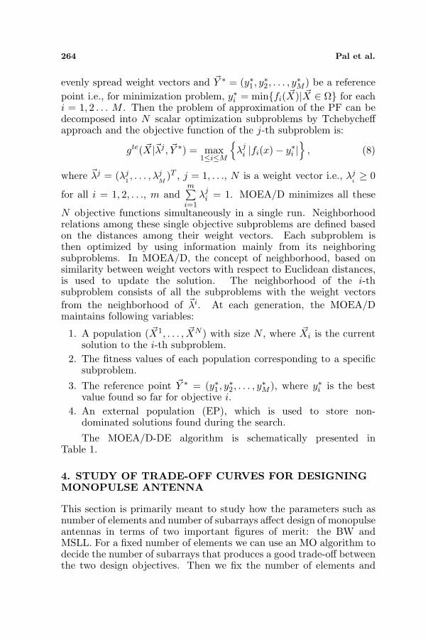
Fixing the number of elements to 20, we run MOEA/D-DE varying thenumber of subarrays P from 2 to 10 in steps of 2. The correspondingapproximated PFs have been shown in Figure 2.

A close inspection of Figure 2 shows that the best trade-off can beachieved for 10 subarrays as points near the knee of the approximatedPF are closest to the origin corresponding to least values of MSLL andBW in comparison to the trade-off curves obtained with other numbersof subarrays. The best compromise solution is chosen from the PFsusing the fuzzy based method as described. The solution for P = 6 is

5 10 15 20 25 30 35-70

-60

-50

-40

-30

-20

-10

0

Beamwidth in Degrees

Maxim

um

Sid

elo

be L

evel in

dB

N=10, P=2

N=10, P=4

N=10, P=6

N=10, P=8

N=10, P=10

Figure 2. Trade-off curves for 20 element array (N = 10).


also sufficiently good. Beamwidth of 15.95 and MSLL of −38.78 dBis obtained compared to 15.35 and −40.78 dB for 10 subarrays. Wecould go for 6 subarrays because it gives sufficiently low beamwidthand MSLL. Increasing the number of subarrays improves the resultslightly at the cost of design complexity.

4.2. Case 2: 40 Element Array

Figures 3 and 4 show the trade-off curve obtained for 40 element arraywith number of subarrays = 2, 4, 6, 8, 10, 12, 14, 16, 18, and 20. Wehave presented the best compromise solution in Table 3. In comparisonto 20 element array it is clearly evident that 40 element array patternshave very narrow beamwidth. From Table 3 we see that with lessernumber of subarrays sufficiently low SLLs are not obtained. MinimumMSLL is obtained for 20 subarrays but it is only 3.69 dB lower thanthat for 14 subarrays and 0.69 dB lower than for 12 subarrays. So fordesigning a 40 element monopulse array with no exact specifications assuch, we could go for 14 or 12 subarrays because sufficiently low MSLLis achieved with narrow beamwidth for these cases.

4.3. Case 3: Number of Subarrays Constant

Here we have fixed the number of subarrays to P = 8. In this casewe can observe that keeping P constant increasing N decreases thebeamwidth steadily.

We see that till N = 14 MSLL is steadily minimized. Increasingthe number of elements further leads to narrower beamwidth.

2 4 6 8 10 12 14 16 18 20-40

-35

-30

-25

-20

-15

-10

-5

0


Maxim

um

Sid

elo

be L

evel in

dB

N=20, P=2

N=20, P=4

N=20, P=6N=20, P=8

N=20, P=10

Figure 3. Trade-off curve for 40 element array (N = 20, P =2, 4, 6, 8, 10).

268 Pal et al.

4 6 8 10 12 14 16-45

-40

-35

-30

-25

-20

-15

-10


Maxim

um

Sid

elo

be L

evel in

dB

N=20, P=12

N=20, P=14

N=20, P=16

N=20, P=18

N=20, P=20

Figure 4. Trade-off curves for 40 element array (N = 20, P =12, 14, 16, 18, 20).

Table 2. Optimal compromise table for 20 element array.

No. of Subarrays (P ) BW MSLL

2 11.54 −17.1

4 12.04 −24.98

6 15.95 −38.78

8 15.96 −40.41

10 15.35 −40.78

Table 3. Optimal compromise table for 40 element array.

No. of Subarrays (P ) BW MSLL

2 5.72 −18.86

4 5.48 −20.33

6 6.31 −29.16

8 11.44 −29.74

10 9.63 −30.32

12 14.89 −40.45

14 12.64 −37.45

16 11.3 −39.1

18 11.26 −38.6

20 12.6 −41.14


Thus keeping subarrays constant and increasing N decreases thebeamwidth but increases Maximum Sidelobe Level. MaximumSidelobe suppression is obtained for N = 10 and minimum beamwidthis obtained with N = 18. For N = 20 some solutions have extremelylow beamwidth but not so low MSLL. The best compromise solutionfor N = 20 has higher beamwidth but much lower MSLL compared tothat for N = 18.

4.4. Case 4: P/N Constant

In this case we show how the quality of design improves whenthe number of elements and subarrays are increased in the sameproportion. As N and P increases the improvement in Beamwidth andMSLL is clear from the Optimal Compromise Table. The Beamwidthimproves from 20.17 for N = 5, P = 3 to 14.89 for N = 20, P = 12.MSLL improves from −13.93 dB for N = 5, P = 3 to −42.45 dB forN = 20, P = 12. From Figure 6 it is also evident that the improvementof solution is less pronounced as N and P increases as the PFs get closerand closer with increase in N and P . It can also be observed from thePFs that greater number of elements can achieve a particular sidelobelevel in lesser beamwidth.

The aim of this section was to investigate how the optimalcombination of two vital parameters related to the design problem viz.number of elements and number of subarrays can be estimated usingan MO algorithm. The next section is devoted to the actual designof the monopulse array using MOEA/D-DE with the subarray weightsand the element grouping kept as decision variables.

4 6 8 10 12 14 16 18 20 22-45

-40

-35

-30

-25

-20

-15

-10

-5


Maxim

um

Sid

elo

be L

evel in

dB

N=8, P=8

N=10, P=8

N=12, P=8

N=14, P=8

N=16, P=8

N=18, P=8

N=20, P=8

Figure 5. Trade-off curve for fixed number of subarrays (P = 8).

270 Pal et al.

0 5 10 15 20 25 30 35-70

-60

-50

-40

-30

-20

-10

0


Maxim

um

Sid

elo

be L

evel in

dB

N=5, P=3

N=10, P=6

N=15, P=9

N=20, P=12

Figure 6. Trade-off curve for P/N = 0.6.

5. DESIGNING MONOPULSE ANTENNA ARRAYSWITH MOEA/D-DE

Suppose we have the task of designing a 20 element monopulse antennaarray with the following specifications:

i) SLL of sum pattern = −25 dBii) MSLL of difference pattern = −27 dBiii) Beamwidth of difference pattern = 12

A good design would aim at minimizing the cost and complexitysimultaneously. Thus, it follows that we should go for the minimumnumber of subarrays that meet the above design specifications for20 element array. This can be easily achieved by a multi-objectiveoptimization approach. We can easily generate a sum-pattern thatmeets the design specification using a standard technique like Dolph-Chebyshev array design. Then we utilize the sum pattern excitationsto obtain the difference pattern excitations by appropriate subarrayweighting and grouping configuration. We generated approximatedPFs by running MOEA/D-DE for all possible number of subarrays tillwe meet the design specification.

Figure 7 shows the approximated PFs for N = 10 and P = 2, 3, 4and 5. The design specifications were met for 5 subarrays as isevident from the figure. The Pareto curve consists of points each ofwhich corresponds to a specific subarray grouping and weighting. Thedesired point on the Pareto curve has the following subarray weights0.6607, 0.7228, 0.3671, 0.1175, 1 and subarray grouping configuration4, 3, 1, 2, 0, 5, 0, 5, 0, 3.


7 8 9 10 11 12 13 14 15 16 17-35

-30

-25

-20

-15

-10

-5

0


Maxim

um

Sid

elo

be L

evel in

dB

N=10, P=2N=10, P=3N=10, P=4N=10, P=5

Desired point

Figure 7. Trade-off curves for 20 element design.

We also consider another set of design specifications for narrowbeamwidth and low SLL applications:

i) No. of elements = 40ii) SLL of sum pattern = −25 dBiii) MSLL of difference pattern = −30 dBiv) Beamwidth of difference pattern = 7.

Figure 8 shows the approximated PFs obtained with MOEA/D-DE for N = 20 and P = 2, 3, 4, 5 and 6. The design specificationswere met with 6 subarrays as is evident from the figure. The de-sired point on the Pareto curve has the following subarray weights0.6095, 0.1, 0.2581, 0.4724, 0.9831, 0.7018 and subarray grouping con-figuration 2, 3, 3, 4, 1, 6, 6, 5, 0, 0, 0, 5, 0, 0, 5, 1, 6, 1, 1, 4. Thus multi-objective design provides an extremely straightforward method for de-signing monpulse antenna arrays which can be taken up the antennadesigners for their purpose.

6. COMPARATIVE STUDY WITH OTHER DESIGNMETHODS

In this section, we compare the design results obtained with MOEA/D-DE with the Hybrid Contiguous Partition Method (HPCM) [12, 13]and two single-objective optimization algorithms namely DE and PSO.For DE and PSO we followed the same hybrid real/integer codingas reported in [7, 8]. For DE the parametric setup is also taken

272 Pal et al.

3 3.5 4 4.5 5 5.5 6 6.5 7 7.5-35

-30

-25

-20

-15

-10

-5

0


Maxim

um

Sid

elo

be L

evel in

dB

N=20, P=2

N=20, P=3

N=20, P=4

N=20, P=5

N=20, P=6

Desired solution

Figure 8. Trade-off curves for 40 element design.

Table 4. Optimal compromise table for 8 subarrays.

No. of Elements/2 (N) BW MSLL8 14.75 −26.2510 15.96 −40.4112 14.98 −38.4114 14.75 −36.1116 9.63 −27.9818 7.52 −23.9920 11.44 −29.74

Table 5. Optimal compromise table for P/N = 0.6.

N P BW MSLL5 3 20.17 −13.9310 6 15.95 −38.7815 9 15.11 −39.5620 12 14.89 −40.45

from [8]. For PSO, we used swarm size = 200, acceleration coefficientsC1 = C2 = 2.00, inertia weight ω linearly decreasing from 0.9 to 0.4and for dth component of maximum velocity vd,max = 0.9 ∗ rd whererd is the difference between the maximum and minimum values of thedth decision variable.


Below we provide the results for three instantiations of the designproblem corresponding to three different numbers of subarrays. Thesum pattern corresponds to a Dolph-Chebyshev array with distancebetween elements d = λ/2 and SLL = −25 dB. The objective functionfor single-objective algorithms was taken as f1 + f2 where f1 and f2

are given by (5a) and (5b).HCPM was run according to the guidelines given in Rocca et

al. [12]. The reference Zolotarev pattern for Case A and Case B wascharacterized by SLLref = −25 dB and for Case C SLLref = −42 dBwas assumed. Note that MOEA/D-DE, PSO and DE were run up to3× 105 FEs for all problems. As results we provide the best solutionsfound in 25 independent trials of each algorithm. The approximatedPareto curves for MOEA/D-DE were first obtained for the three caseswhich are shown in Figure 9. Then the best compromise solution waschosen by the fuzzy membership based method described in Section 4.The details of the best compromise solution are tabulated along withresults obtained by other competing algorithms. The array patternsare also plotted for demonstrating the viability of our approach.

7 8 9 10 11 12 13 14 15 16 17-45

-40

-35

-30

-25

-20

-15

-10

-5


Maxim

um

Sid

elo

be L

evel in

dB

N=10, P=3

N=10, P=5

N=10, P=8

Figure 9. Trade-off curve for comparative results section.

274 Pal et al.

6.1. Case A: 20 Elements, 3 Subarrays

Table 6. Subarray configuration (Case A).

Algorithms c1 c2 c3 c4 c5 c6 c7 c8 c9 c10

MOEA/D-DE 3 2 1 1 0 0 0 0 0 2HCPM 3 3 1 1 2 2 2 2 2 3

DE 1 1 3 2 2 2 2 2 2 2PSO 3 2 1 1 1 0 1 2 2 2

Table 7. Subarray weights (Case A).

Algorithms g1 g2 g3

MOEA/D-DE 0.6513 0.3589 0.1079HCPM 0.5211 1 0.2963

DE 0.2249 0.9938 0.4810PSO 0.7763 0.7564 0.1007

Table 8. Design objectives achieved (Case A).

Objectives MOEA/D-DE HCPM DE PSOBW (degrees) 11.32 11.56 12.81 11.438

MSLL −24.87 −18.12 −13.45 −14.97

-100 -80 -60 -40 -20 0 20 40 60 80 100-60

-50

-40

-30

-20

-10

0

Elevation angle (deg)

Gain

(d

B)

MOEA/D-DE

HCPM

DE

PSO

Figure 10. Normalized patterns for 20 elements array (Case A).


6.2. Case B: 20 Elements, 5 Subarrays

Table 9. Subarray configuration (Case B).


MOEA/D-DE 4 3 1 2 0 5 0 5 0 3HCPM 5 2 1 1 4 4 3 3 1 5

DE 3 2 1 4 4 5 4 1 3 3PSO 3 3 1 0 2 2 5 4 0 1

Table 10. Subarray weights (Case B).

Algorithms g1 g2 g3 g4 g5

MOEA/D-DE 0.607 0.723 0.367 0.117 1.00HCPM 0.681 0.385 0.999 1.000 0.182

DE 0.734 0.393 0.171 0.991 0.985PSO 0.641 1.000 0.351 1.000 0.843

Table 11. Design objectives achieved (Case B).

Objectives MOEA/D-DE HCPM DE PSOBW(degrees) 12.04 12.34 13.846 13.224

MSLL −26.95 −24.24 −23.73 −19.11

-100 -80 -60 -40 -20 0 20 40 60 80 100-80

-70

-60

-50

-40

-30

-20

-10

0


Gain

(d

B)

MOEA/D-DE

HCPM

DE

PSO

Figure 11. Normalized patterns for 20 elements array (Case B).

276 Pal et al.

6.3. Case C: 20 Elements, 8 Subarrays

Table 12. Subarray configuration (Case C).


MOEA/D-DE 5 7 3 2 6 1 4 4 6 8HCPM 2 7 1 5 4 6 6 3 8 5

DE 6 7 1 5 2 3 3 5 8 4PSO 6 7 1 2 5 3 8 5 7 4

Table 13. Subarray weights (Case C).

Algorithms g1 g2 g3 g4 g5 g6 g7 g8

MOEA/D-DE 0.8056 0.5903 0.4408 0.8521 0.1000 0.7190 0.2824 0.7012

HCPM 0.5041 0.1012 0.9951 0.8241 0.6646 0.9235 0.3100 0.8191

DE 0.4757 0.6877 0.8107 0.1205 0.6953 0.1089 0.2885 0.3448

PSO 0.4744 0.6880 0.8189 0.1195 0.6937 0.1045 0.2287 0.8018

Table 14. Design objectives achieved (Case C).

Objectives MOEA/D-DE HCPM DE PSOBW(degrees) 15.96 16.01 16.02 15.98

MSLL −40.41 −37.76 −28.49 −27.58

-100 -80 -60 -40 -20 0 20 40 60 80 100-100

-90

-80

-70

-60

-50

-40

-30

-20

-10

0


Gain

(dB

)

MOEA/D-DE

HCPM

DE

PSO

Figure 12. Normalized patterns for 20 elements array (Case C).


The subarray grouping configuration for three cases is provided inTables 6, 9 and 12. The subarray weights for the three cases are givenin Tables 7, 10 and 13. A keen observation of Tables 8, 11 and 14 andalso Figures 10–12 show that in all test cases, MOEA/D-DE achievesmuch better design objectives as well as array factors with lower MSLLin comparison with both the single-objective algorithms — DE, PSO,and HCPM.

7. CONCLUSION

This article has presented a new approach to the synthesis problemof the difference patterns of monopulse antenna arrays in a multi-objective optimization framework. One of the most recent and best-known MO algorithms, called MOEA/D-DE, has been applied overdifferent instances of the design problem, keeping minimum MaximumSidelobe Level (MSLL) and principal lobe Beam Width (BW) as twodesign-objectives to be simultaneously achieved. Through extensivesimulation experiments, we illustrated that this design method can beadopted by an antenna designer to detect an optimal combination ofthe number of elements (2N) and number of subarrays (P ) such thatthe best trade-off between quality of solution and design complexity ismaintained.

The subarray grouping information and weights are obtained fromthe best compromise solution of the approximated PFs correspondingto N and P as determined before. The best compromise solution forN = 10 and P = 3, 5, and 8 are obtained from their approximated PFsand the figure of merit of solution (i.e., MSLL and BW) are shown tobeat those obtained with two well-known single-objective optimizationalgorithms DE, PSO, and HCPM. We have also demonstrated that theoptimal 20 element array design should be with 6 subarrays. Increasingthe number of subarrays increases the complexity of design withoutimproving the quality of solution appreciably. In conclusion we can saythat MO algorithms have a dual role in the design process viz. theycan be used for fixing N and P as well as for determining the subarrayconfiguration and subarray weights. The method of design presentedin this paper can be directly put to use by the antenna designers.

Finally, we would like to point out that in this article we presentedonly one of the possible synthesis problems. There may be someother design objectives based on different formulations and it will beinteresting to extend the multi-objective approach to those in future.

278 Pal et al.

REFERENCES

1. Skolnik, I. M., Radar Handbook, McGraw-Hill, 1990.2. Sherman, S. M., Monopulse Principles and Techniques, Artech

House, 1984.3. Bayliss, E. T., “Design of monopulse antenna difference patterns

with low sidelobes,” Bell Syst. Tech. J., Vol. 47, 623–650, 1968.4. McNamara, D. A., “Synthesis of sum and difference patterns for

two section monopulse arrays,” Proc. Inst. Elect. Eng., Part H,Vol. 135, No. 6, 371–374, Dec. 1988.

5. Elliott, R. S., Antenna Theory and Design, Prentice Hall,Englewood Cliffs, NJ, 1981.

6. Lopez, P., J. A. Rodrıguez, F. Ares, and E. Moreno, “Subarrayweighting for the difference patterns of monopulse antennas:Joint optimization of subarray configurations and weights,” IEEETrans. Antennas Propag., Vol. 49, No. 11, 1606–1608, Nov. 2001.

7. Caorsi, S., A. Massa, M. Pastorino, and A. Randazzo,“Optimization of the difference patterns for monopulse antennasby a hybrid real/integer coded differential evolution method,”IEEE Trans. Antennas Propag., Vol. 53, No. 1, 372–376,Jan. 2005.

8. Massa, A., M. Pastorino, and A. Randazzo, “Optimization of thedirectivity of a monopulse antenna with a subarray weighting bya hybrid differential evolution method,” IEEE Antennas WirelessPropag. Lett., Vol. 5, 155–158, 2006.

9. D’Urso, M., T. Isernia, and E. F. Meliado, “An effective hybridapproach for the optimal synthesis of monopulse antennas,” IEEETrans. Antennas Propag., Vol. 55, 1059–1066, Apr. 2007.

10. Manica, L., P. Rocca, A. Martini, and A. Massa, “Aninnovative approach based on a tree-searching algorithm for theoptimal matching of independently optimum sum and differenceexcitations,” IEEE Trans. Antennas Propag., Vol. 56, 58–66,Jan. 2008.

11. Rocca, P., L. Manica, and A. Massa, “Synthesis of monopulse an-tennas through iterative contiguous partition method,” Electron.Lett., Vol. 43, No. 16, 854–856, Aug. 2007.

12. Rocca, P., L. Manica, R. Azaro, and A. Massa, “A hybridapproach to the synthesis of subarrayed monopulse linear arrays,”IEEE Trans. Antennas Propag., Vol. 57, 280–283, Jan. 2009.

13. Rocca, P., L. Manica and A. Massa, “Hybrid approach for sub-arrayed monopulse antenna synthesis,” Electron. Lett., Vol. 44,


No. 2, Jan. 2008.14. Rocca, P., L. Manica, and A. Massa, “An improved excita-

tion matching method based on an ant colony optimizationfor suboptimal-free clustering in sum-difference compromise syn-thesis,” IEEE Trans. Antennas Propag., Vol. 57, 2297–2306,Aug. 2009.

15. Rocca, P., L. Manica, and A. Massa, “An effective excitationmatching method for the synthesis of optimal compromisesbetween sum and difference patterns in planar arrays,” ProgressIn Electromagnetic Research B, Vol. 3, 115–130, 2008.

16. Rocca, P., L. Manica, and A. Massa, “Directivity optimization inplanar sub-arrayed monopulse antenna,” Progress In Electromag-netics Research Letters, Vol. 4, 1–7, 2008.

17. Manica, L., P. Rocca, and A. Massa, “Design of sub-arrayed lineararray antennas with SLL control based on an excitation matchingapproach,” IEEE Trans. Antennas Propagat., Vol. 57, No. 6, 1684–1691, Jun. 2009.

18. Manica, L., P. Rocca, and A. Massa, “A fast graph-searchingalgorithm enabling the efficient synthesis of sub-arrayed planarmonopulse antennas,” IEEE Trans. Antennas Propagat., Vol. 57,No. 3, 652–664, Mar. 2009.

19. Manica, L., P. Rocca, and A. Massa, “An excitation matchingprocedure for sub-arrayed monopulse arrays with maximumdirectivity,” IET Radar, Sonar, and Navigation, Vol. 3, No. 1,42-48, Feb. 2009.

20. Manica, L., P. Rocca, M. Pastorino, and A. Massa, “Boresightslope optimization of sub-arrayed linear arrays through thecontiguous partition method,” IEEE Antenna and PropagationLetters, Vol. 8, 253–257, 2008.

21. Rocca, P., L. Manica, A. Martini, and A. Massa, “Compromisesum-difference optimization through the iterative contiguouspartition method,” IET Microwaves, Antennas, and Propagation,Vol. 3, No. 2, 348–361, 2009.

22. Massa, A., M. Pastorino, and A. Randazzo, “Optimization of thedirectivity of a monopulse antenna with a subarray weighting bya hybrid differential evolution method,” IEEE Antennas WirelessPropag. Lett., Vol. 5, 155–158, 2006.

23. Deb, K., Multi-objective Optimization Using EvolutionaryAlgorithms, John Wiley & Sons, 2001.

24. Li, H. and Q. Zhang, “Multiobjective optimization problems withcomplicated pareto sets, MOEA/D and NSGA-II,” IEEE Trans.

280 Pal et al.

on Evolutionary Computation, Vol. 12, No 2, 284–302, 2009.25. Zhang, Q., W. Liu, and H. Li, “The performance of a new

MOEA/D on CEC09 MOP test instances,” Proceedings of theEleventh Conference on Congress on Evolutionary Computation,(Trondheim, Norway, May 18–21, 2009). 203–208, IEEE Press,Piscataway, NJ, 2009.

26. Zhang, Q., A. Zhou, S. Z. Zhao, P. N. Suganthan, W. Liu, andS. Tiwari, “Multiobjective optimization test instances for the CEC2009 special session and competition,” Technical Report CES-887,University of Essex and Nanyang Technological University, 2008.

27. Storn, R. and K. Price, “Differential evolution — A simple andefficient heuristic for global optimization over continuous spaces,”Journal of Global Optimization, Vol. 11, No. 4, 341–359, 1997.

28. Price, K., R. Storn, and J. Lampinen, Differential Evolution — APractical Approach to Global Optimization, Springer, Berlin, 2005.

29. Abido, M. A., “A novel multiobjective evolutionary algorithm forenvironmental/economic power dispatch,” Electric Power SystemsResearch, Vol. 65, 71–81, Elsevier, 2003.

30. Kennedy, J., R. C. Eberhart, and Y. Shi, Swarm Intelligence,Morgan Kaufmann, San Francisco, CA, 2001.

31. Dolph, C. L., “A current distribution for broadside arrays,” Proc.IRE, Vol. 34, 335–348, Jun. 1946.

32. Abramovitz, M. and I. A. Stegun, Handbook of MathematicalFunctions, Dover Publications, New York, 1965.

33. Abraham, A., L. C. Jain, and R. Goldberg, Evolutionary Mul-tiobjective Optimization: Theoretical Advances and Applications,Springer Verlag, London, 2005.

34. Coello Coello, C. A., G. B. Lamont, and D. A. van Veldhuizen,Evolutionary Algorithms for Solving Multi-objective Problems,Springer, 2007.

35. Zhang, Q. and H. Li, “MOEA/D: A multi-objective evolutionaryalgorithm based on decomposition,” IEEE Trans. on EvolutionaryComputation, Vol. 11, No. 6, 712–731, 2007.

36. Miettinen, K., Nonlinear Multiobjective Optimization, KuluwerAcademic Publishers, 1999.

Documents

SYNTHESIS OF DIFFERENCE PATTERNS FOR MONOPULSE ANTENNAS ... · SYNTHESIS OF DIFFERENCE PATTERNS FOR MONOPULSE ANTENNAS WITH OPTIMAL COMBINA- ... antenna array by observing the shape