Synthesis Lectures on Communication Networks

Series ISSN: 1935-4185

Synthesis Lectures onCommunication Networks


store.morganclaypool.comR. Srikant, Series Editor

WA

LRA

ND

• PAR

EKH

CO

MM

UN

ICAT

ION

NE

TW

OR

KS, 2N

D ED

ITIO

N

MO

RG

AN

& C

LAY

PO

OL

Series Editor: R. Srikant, University of Illinois at Urbana-Champaign

Communication NetworksA Concise Introduction, Second EditionJean Walrand, University of California, BerkeleyShyam Parekh, AT&T Labs Research and University of California, Berkeley (Adjunct)

After an overview of the Internet design and operating principles, the book presents the main ideas behind Ethernet, WiFi networks, routing, internetworking, and TCP. It then covers models, the key aspects of the modern LTE based wireless networks, QoS, and the prevalent physical layer technologies. The book then discusses content delivery and peer-to-peer networks, sensor networks, distributed algorithms, Byzantine agreement, source compression, SDN and NFV, and Internet of Things.

“...informed, informative, and useful to students, faculty, and practitioners in the field.” – Anthony Ephremides, University of Maryland

“A concise and refreshing treatment that focuses on the fundamental principles …” – Massimo Franceschetti, University of California, San Diego

“The most important principles of communication network design, with emphasis on the Internet, in a crisp and clear fashion.” – Bruce Hajek, University of Illinois at Urbana-Champaign

“Conceptual clarity, simplicity of explanation, and brevity are the soul of this book. I wish there had been such a book when I was learning about communication networks.” – P.R. Kumar, Texas A&M

“A holistic account of this critical yet complex infrastructure and explains the essential ideas clearly and precisely … It is the best introduction to networking …” – Steven Low, Caltech

“An amazing book. … Jean and Shyam are in the unique position for writing this book … It is certainly a must-have book.” – Lei Ying, Arizona State University

About SYNTHESIS

This volume is a printed version of a work that appears in the Synthesis Digital Library of Engineering and Computer Science. Synthesis books provide concise, original presentations of important research and development topics, published quickly, in digital and print formats.

ii

Praise forCommunicationNetworks: A Concise IntroductionThis book is a welcome addition to the Networking literature. It presents a comprehensive set oftopics from an innovative and modern viewpoint that observes the rapid development that thefield has undergone. It is informed, informative, and useful to students, faculty, and practitionersin the field. This book is a must have!

-Anthony Ephremides, University of Maryland

Computer networks are extremely complex systems, and university-level textbooks often containlengthy descriptions of them that sacrifice basic conceptual understanding in favor of detailedoperational explanations. Walrand and Parekh depart from this approach, offering a concise andrefreshing treatment that focuses on the fundamental principles that students can (and should)carry forward in their careers.The new edition has been updated to cover the latest developmentsand is of great value for teaching a first upper-division course on computer networks.

-Massimo Franceschetti, University of California, San Diego

The book presents the most important principles of communication network design, with em-phasis on the Internet, in a crisp and clear fashion. Coverage extends from physical layer issuesthrough the key distributed applications. The book will be a valuable resource to students, in-structors, and practitioners for years to come.

-Bruce Hajek, University of Illinois at Urbana-Champaign

Conceptual clarity, simplicity of explanation, and brevity are the soul of this book. It covers avery broad swathe of contemporary topics, distills complex systems into their absolutely basicconstituent ideas, and explains each idea clearly and succinctly. It is a role model of what aclassroom text should be. I wish there had been such a book when I was learning about com-munication networks.

-P. R. Kumar, Texas A&MUniversity

PRAISE FORCOMMUNICATIONNETWORKS: A CONCISE INTRODUCTION iii

This book focuses on the basic principles that underlie the design and operation of the Inter-net. It provides a holistic account of this critical yet complex infrastructure and explains theessential ideas clearly and precisely without being obscured by unessential implementation oranalytical details. It is the best introduction to networking from which more specialized treat-ment of various topics can be pursued.

-Steven Low, California Institute of Technology (Caltech)

Communication Networks: A Concise Introduction by Jean Walrand and Shyam Parekh is an amaz-ing book. Jean and Shyam are in the unique position for writing this book because of the foun-dational contributions they made to the area and their many years of teaching this course atUC Berkeley. This book covers many important topics ranging from the architecture of the In-ternet, to today’s wireless technologies, and to emerging topics such as SDN and IoT. For eachtopic, the book focuses on the key principles and core concepts, and presents a concise discussionof how these principles are essential to scalable and robust communication networks. Mathe-matical tools such as Markov chains and graph theory are introduced at a level that is easilyunderstandable but also adequate for modeling and analyzing the key components of communi-cation networks. The comprehensive coverage of core concepts of communication networks andthe intuition/principle-driven approach make this book the best textbook for an introductorycourse in communication networks for those students who are interested in pursuing researchin this field. It is certainly a must-have book for students and researchers in the field.

-Lei Ying, Arizona State University


EditorR. Srikant,University of Illinois at Urbana-Champaign

Founding Editor EmeritusJean Walrand,University of California, Berkeley

Synthesis Lectures on Communication Networks is an ongoing series of 50- to 100-page publicationson topics on the design, implementation, and management of communication networks. Eachlecture is a self-contained presentation of one topic by a leading expert. The topics range fromalgorithms to hardware implementations and cover a broad spectrum of issues from security tomultiple-access protocols. The series addresses technologies from sensor networks to reconfigurableoptical networks.The series is designed to:

• Provide the best available presentations of important aspects of communication networks.

• Help engineers and advanced students keep up with recent developments in a rapidlyevolving technology.

• Facilitate the development of courses in this field

Communication Networks: A Concise Introduction, Second EditionJean Walrand and Shyam Parekh2017

BATS Codes: Theory and PracticeShenghao Yang and Raymond W. Yeung2017

Analytical Methods for Network Congestion ControlSteven H. Low2017

Advances in Multi-Channel Resource Allocation: Throughput, Delay, and ComplexityBo Ji, Xiaojun Lin, Ness B. Shroff2016

viA Primer on Physical-Layer Network CodingSoung Chang Liew, Lu Lu, and Shengli Zhang2015

Sharing Network ResourcesAbhay Parekh and Jean Walrand2014

Wireless Network PricingJianwei Huang and Lin Gao2013

Performance Modeling, Stochastic Networks, and Statistical Multiplexing, SecondEditionRavi R. Mazumdar2013

Packets with Deadlines: A Framework for Real-Time Wireless NetworksI-Hong Hou and P.R. Kumar2013

Energy-Efficient Scheduling under Delay Constraints for Wireless NetworksRandall Berry, Eytan Modiano, and Murtaza Zafer2012

NS Simulator for BeginnersEitan Altman and Tania Jiménez2012

Network Games: Theory, Models, and DynamicsIshai Menache and Asuman Ozdaglar2011

An Introduction to Models of Online Peer-to-Peer Social NetworkingGeorge Kesidis2010

Stochastic Network Optimization with Application to Communication and QueueingSystemsMichael J. Neely2010

Scheduling and Congestion Control for Wireless and Processing NetworksLibin Jiang and Jean Walrand2010

viiPerformance Modeling of Communication Networks with Markov ChainsJeonghoon Mo2010

Communication Networks: A Concise IntroductionJean Walrand and Shyam Parekh2010

Path Problems in NetworksJohn S. Baras and George Theodorakopoulos2010

Performance Modeling, Loss Networks, and Statistical MultiplexingRavi R. Mazumdar2009

Network SimulationRichard M. Fujimoto, Kalyan S. Perumalla, and George F. Riley2006

Copyright © 2018 by Morgan & Claypool

All rights reserved. No part of this publication may be reproduced, stored in a retrieval system, or transmitted inany form or by anymeans—electronic, mechanical, photocopy, recording, or any other except for brief quotationsin printed reviews, without the prior permission of the publisher.

Communication Networks: A Concise Introduction, Second Edition

Jean Walrand and Shyam Parekh

www.morganclaypool.com

ISBN: 9781627058872 paperbackISBN: 9781627058995 ebookISBN: 9781681732060 epubISBN: 9781681736150 hardcover

DOI 10.2200/S00804ED2V01Y201709CNT020

A Publication in the Morgan & Claypool Publishers seriesSYNTHESIS LECTURES ON COMMUNICATION NETWORKS

Lecture #20Series Editor: R. Srikant, University of Illinois at Urbana-ChampaignFounding Editor Emeritus: Jean Walrand, University of California, BerkeleySeries ISSNPrint 1935-4185 Electronic 1935-4193

www.morganclaypool.com

Communication NetworksA Concise IntroductionSecond Edition

Jean WalrandUniversity of California, Berkeley

Shyam ParekhAT&T Labs Research and University of California, Berkeley (Adjunct)

SYNTHESIS LECTURES ON COMMUNICATION NETWORKS #20

CM&

cLaypoolMorgan publishers&

ABSTRACT TO THE SECOND EDITIONThis book results from many years of teaching an upper division course on communication net-works in the EECS department at the University of California, Berkeley. It is motivated by theperceived need for an easily accessible textbook that puts emphasis on the core concepts behindcurrent and next generation networks. After an overview of how today’s Internet works and adiscussion of the main principles behind its architecture, we discuss the key ideas behind Eth-ernet, WiFi networks, routing, internetworking, and TCP. To make the book as self-containedas possible, brief discussions of probability and Markov chain concepts are included in the ap-pendices. This is followed by a brief discussion of mathematical models that provide insight intothe operations of network protocols. Next, the main ideas behind the new generation of wirelessnetworks based on LTE, and the notion of QoS are presented. A concise discussion of the phys-ical layer technologies underlying various networks is also included. Finally, a sampling of topicsis presented that may have significant influence on the future evolution of networks, includingoverlay networks like content delivery and peer-to-peer networks, sensor networks, distributedalgorithms, Byzantine agreement, source compression, SDN and NFV, and Internet of Things.

KEYWORDSInternet, Ethernet, WiFi, Routing, Bellman-Ford algorithm, Dijkstra algorithm,TCP, Congestion Control, Flow Control, QoS, LTE, Peer-to-Peer Networks,SDN, NFV, IoT

xi

ContentsPraise forCommunication Networks: A Concise Introduction . . . . . . . . . . . . . . . . ii

Preface . . . . . . . . . . . . . . . . . . . . . . . . . . . . . . . . . . . . . . . . . . . . . . . . . . . . . . . . . . xix

1 The Internet . . . . . . . . . . . . . . . . . . . . . . . . . . . . . . . . . . . . . . . . . . . . . . . . . . . . . . . 11.1 Basic Operations . . . . . . . . . . . . . . . . . . . . . . . . . . . . . . . . . . . . . . . . . . . . . . . . . 1

1.1.1 Hosts, Routers, Links . . . . . . . . . . . . . . . . . . . . . . . . . . . . . . . . . . . . . . . . 11.1.2 Packet Switching . . . . . . . . . . . . . . . . . . . . . . . . . . . . . . . . . . . . . . . . . . . . 11.1.3 Addressing . . . . . . . . . . . . . . . . . . . . . . . . . . . . . . . . . . . . . . . . . . . . . . . . . 21.1.4 Routing . . . . . . . . . . . . . . . . . . . . . . . . . . . . . . . . . . . . . . . . . . . . . . . . . . . 31.1.5 Error Detection . . . . . . . . . . . . . . . . . . . . . . . . . . . . . . . . . . . . . . . . . . . . . 41.1.6 Retransmission of Erroneous Packets . . . . . . . . . . . . . . . . . . . . . . . . . . . . 51.1.7 Congestion Control . . . . . . . . . . . . . . . . . . . . . . . . . . . . . . . . . . . . . . . . . . 51.1.8 Flow Control . . . . . . . . . . . . . . . . . . . . . . . . . . . . . . . . . . . . . . . . . . . . . . . 5

1.2 DNS, HTTP, and WWW. . . . . . . . . . . . . . . . . . . . . . . . . . . . . . . . . . . . . . . . . . 61.2.1 DNS . . . . . . . . . . . . . . . . . . . . . . . . . . . . . . . . . . . . . . . . . . . . . . . . . . . . . 61.2.2 HTTP and WWW. . . . . . . . . . . . . . . . . . . . . . . . . . . . . . . . . . . . . . . . . . 6

1.3 Summary . . . . . . . . . . . . . . . . . . . . . . . . . . . . . . . . . . . . . . . . . . . . . . . . . . . . . . . 61.4 Problems . . . . . . . . . . . . . . . . . . . . . . . . . . . . . . . . . . . . . . . . . . . . . . . . . . . . . . . . 71.5 References . . . . . . . . . . . . . . . . . . . . . . . . . . . . . . . . . . . . . . . . . . . . . . . . . . . . . . . 7

2 Principles . . . . . . . . . . . . . . . . . . . . . . . . . . . . . . . . . . . . . . . . . . . . . . . . . . . . . . . . . . 92.1 Sharing . . . . . . . . . . . . . . . . . . . . . . . . . . . . . . . . . . . . . . . . . . . . . . . . . . . . . . . . . 92.2 Metrics . . . . . . . . . . . . . . . . . . . . . . . . . . . . . . . . . . . . . . . . . . . . . . . . . . . . . . . . 10

2.2.1 Link Rate . . . . . . . . . . . . . . . . . . . . . . . . . . . . . . . . . . . . . . . . . . . . . . . . . 102.2.2 Link Bandwidth and Capacity . . . . . . . . . . . . . . . . . . . . . . . . . . . . . . . . 112.2.3 Delay . . . . . . . . . . . . . . . . . . . . . . . . . . . . . . . . . . . . . . . . . . . . . . . . . . . . 122.2.4 Throughput . . . . . . . . . . . . . . . . . . . . . . . . . . . . . . . . . . . . . . . . . . . . . . . 122.2.5 Delay Jitter . . . . . . . . . . . . . . . . . . . . . . . . . . . . . . . . . . . . . . . . . . . . . . . 142.2.6 M/M/1 Queue . . . . . . . . . . . . . . . . . . . . . . . . . . . . . . . . . . . . . . . . . . . . 142.2.7 Little’s Result . . . . . . . . . . . . . . . . . . . . . . . . . . . . . . . . . . . . . . . . . . . . . . 162.2.8 Fairness . . . . . . . . . . . . . . . . . . . . . . . . . . . . . . . . . . . . . . . . . . . . . . . . . . 17

xii2.3 Scalability . . . . . . . . . . . . . . . . . . . . . . . . . . . . . . . . . . . . . . . . . . . . . . . . . . . . . . 18

2.3.1 Location-based Addressing . . . . . . . . . . . . . . . . . . . . . . . . . . . . . . . . . . 182.3.2 Two-level Routing . . . . . . . . . . . . . . . . . . . . . . . . . . . . . . . . . . . . . . . . . . 192.3.3 Best Effort Service . . . . . . . . . . . . . . . . . . . . . . . . . . . . . . . . . . . . . . . . . 202.3.4 End-to-end Principle and Stateless Routers . . . . . . . . . . . . . . . . . . . . . 202.3.5 Hierarchical Naming . . . . . . . . . . . . . . . . . . . . . . . . . . . . . . . . . . . . . . . . 20

2.4 Application and Technology Independence . . . . . . . . . . . . . . . . . . . . . . . . . . . 212.4.1 Layers . . . . . . . . . . . . . . . . . . . . . . . . . . . . . . . . . . . . . . . . . . . . . . . . . . . 21

2.5 Application Topology . . . . . . . . . . . . . . . . . . . . . . . . . . . . . . . . . . . . . . . . . . . . . 222.5.1 Client/Server . . . . . . . . . . . . . . . . . . . . . . . . . . . . . . . . . . . . . . . . . . . . . . 222.5.2 P2P . . . . . . . . . . . . . . . . . . . . . . . . . . . . . . . . . . . . . . . . . . . . . . . . . . . . . 232.5.3 Cloud Computing . . . . . . . . . . . . . . . . . . . . . . . . . . . . . . . . . . . . . . . . . . 232.5.4 Content Distribution . . . . . . . . . . . . . . . . . . . . . . . . . . . . . . . . . . . . . . . 242.5.5 Multicast/Anycast . . . . . . . . . . . . . . . . . . . . . . . . . . . . . . . . . . . . . . . . . . 242.5.6 Push/Pull . . . . . . . . . . . . . . . . . . . . . . . . . . . . . . . . . . . . . . . . . . . . . . . . . 242.5.7 Discovery . . . . . . . . . . . . . . . . . . . . . . . . . . . . . . . . . . . . . . . . . . . . . . . . . 24

2.6 Summary . . . . . . . . . . . . . . . . . . . . . . . . . . . . . . . . . . . . . . . . . . . . . . . . . . . . . . 242.7 Problems . . . . . . . . . . . . . . . . . . . . . . . . . . . . . . . . . . . . . . . . . . . . . . . . . . . . . . . 252.8 References . . . . . . . . . . . . . . . . . . . . . . . . . . . . . . . . . . . . . . . . . . . . . . . . . . . . . . 28

3 Ethernet . . . . . . . . . . . . . . . . . . . . . . . . . . . . . . . . . . . . . . . . . . . . . . . . . . . . . . . . . . 293.1 Typical Installation . . . . . . . . . . . . . . . . . . . . . . . . . . . . . . . . . . . . . . . . . . . . . . . 293.2 History of Ethernet . . . . . . . . . . . . . . . . . . . . . . . . . . . . . . . . . . . . . . . . . . . . . . 29

3.2.1 Aloha Network . . . . . . . . . . . . . . . . . . . . . . . . . . . . . . . . . . . . . . . . . . . . 293.2.2 Cable Ethernet . . . . . . . . . . . . . . . . . . . . . . . . . . . . . . . . . . . . . . . . . . . . 313.2.3 Hub Ethernet . . . . . . . . . . . . . . . . . . . . . . . . . . . . . . . . . . . . . . . . . . . . . 323.2.4 Switched Ethernet . . . . . . . . . . . . . . . . . . . . . . . . . . . . . . . . . . . . . . . . . 33

3.3 Addresses . . . . . . . . . . . . . . . . . . . . . . . . . . . . . . . . . . . . . . . . . . . . . . . . . . . . . . 333.4 Frame . . . . . . . . . . . . . . . . . . . . . . . . . . . . . . . . . . . . . . . . . . . . . . . . . . . . . . . . . 333.5 Physical Layer . . . . . . . . . . . . . . . . . . . . . . . . . . . . . . . . . . . . . . . . . . . . . . . . . . . 343.6 Switched Ethernet . . . . . . . . . . . . . . . . . . . . . . . . . . . . . . . . . . . . . . . . . . . . . . . 35

3.6.1 Example . . . . . . . . . . . . . . . . . . . . . . . . . . . . . . . . . . . . . . . . . . . . . . . . . . 353.6.2 Learning . . . . . . . . . . . . . . . . . . . . . . . . . . . . . . . . . . . . . . . . . . . . . . . . . 353.6.3 Spanning Tree Protocol . . . . . . . . . . . . . . . . . . . . . . . . . . . . . . . . . . . . . . 36

3.7 Aloha . . . . . . . . . . . . . . . . . . . . . . . . . . . . . . . . . . . . . . . . . . . . . . . . . . . . . . . . . 373.7.1 Time-slotted Version . . . . . . . . . . . . . . . . . . . . . . . . . . . . . . . . . . . . . . . 37

xiii3.8 Non-slotted Aloha . . . . . . . . . . . . . . . . . . . . . . . . . . . . . . . . . . . . . . . . . . . . . . . 383.9 Hub Ethernet . . . . . . . . . . . . . . . . . . . . . . . . . . . . . . . . . . . . . . . . . . . . . . . . . . . 38

3.9.1 Maximum Collision Detection Time . . . . . . . . . . . . . . . . . . . . . . . . . . . 383.10 Appendix: Probability . . . . . . . . . . . . . . . . . . . . . . . . . . . . . . . . . . . . . . . . . . . . 39

3.10.1 Probability . . . . . . . . . . . . . . . . . . . . . . . . . . . . . . . . . . . . . . . . . . . . . . . . 403.10.2 Additivity for Exclusive Events . . . . . . . . . . . . . . . . . . . . . . . . . . . . . . . 403.10.3 Independent Events . . . . . . . . . . . . . . . . . . . . . . . . . . . . . . . . . . . . . . . . 413.10.4 Slotted Aloha . . . . . . . . . . . . . . . . . . . . . . . . . . . . . . . . . . . . . . . . . . . . . 413.10.5 Non-slotted Aloha . . . . . . . . . . . . . . . . . . . . . . . . . . . . . . . . . . . . . . . . . 423.10.6 Waiting for Success . . . . . . . . . . . . . . . . . . . . . . . . . . . . . . . . . . . . . . . . . 433.10.7 Hub Ethernet . . . . . . . . . . . . . . . . . . . . . . . . . . . . . . . . . . . . . . . . . . . . . 43


4 WiFi . . . . . . . . . . . . . . . . . . . . . . . . . . . . . . . . . . . . . . . . . . . . . . . . . . . . . . . . . . . . 474.1 Basic Operations . . . . . . . . . . . . . . . . . . . . . . . . . . . . . . . . . . . . . . . . . . . . . . . . 474.2 Medium Access Control (MAC) . . . . . . . . . . . . . . . . . . . . . . . . . . . . . . . . . . . . 48

4.2.1 MAC Protocol . . . . . . . . . . . . . . . . . . . . . . . . . . . . . . . . . . . . . . . . . . . . . 484.2.2 Enhancements for Medium Access . . . . . . . . . . . . . . . . . . . . . . . . . . . . 504.2.3 MAC Addresses . . . . . . . . . . . . . . . . . . . . . . . . . . . . . . . . . . . . . . . . . . . 51

4.3 Physical Layer . . . . . . . . . . . . . . . . . . . . . . . . . . . . . . . . . . . . . . . . . . . . . . . . . . . 524.4 Efficiency Analysis of MAC Protocol . . . . . . . . . . . . . . . . . . . . . . . . . . . . . . . . 53

4.4.1 Single Device . . . . . . . . . . . . . . . . . . . . . . . . . . . . . . . . . . . . . . . . . . . . . . 534.4.2 Multiple Devices . . . . . . . . . . . . . . . . . . . . . . . . . . . . . . . . . . . . . . . . . . . 53

4.5 Recent Advances . . . . . . . . . . . . . . . . . . . . . . . . . . . . . . . . . . . . . . . . . . . . . . . . 574.5.1 IEEE 802.11n—Introduction of MIMO in WiFi . . . . . . . . . . . . . . . . 574.5.2 IEEE 802.11ad—WiFi in Millimeter Wave Spectrum . . . . . . . . . . . . . 584.5.3 IEEE 802.11ac—Introduction of MU-MIMO in WiFi . . . . . . . . . . . 594.5.4 IEEE 802.11ah—WiFi for IoT and M2M . . . . . . . . . . . . . . . . . . . . . . 594.5.5 Peer-to-peer WiFi . . . . . . . . . . . . . . . . . . . . . . . . . . . . . . . . . . . . . . . . . . 60

4.6 Appendix: Markov Chains . . . . . . . . . . . . . . . . . . . . . . . . . . . . . . . . . . . . . . . . . 604.7 Summary . . . . . . . . . . . . . . . . . . . . . . . . . . . . . . . . . . . . . . . . . . . . . . . . . . . . . . 634.8 Problems . . . . . . . . . . . . . . . . . . . . . . . . . . . . . . . . . . . . . . . . . . . . . . . . . . . . . . . 634.9 References . . . . . . . . . . . . . . . . . . . . . . . . . . . . . . . . . . . . . . . . . . . . . . . . . . . . . . 65

xiv

5 Routing . . . . . . . . . . . . . . . . . . . . . . . . . . . . . . . . . . . . . . . . . . . . . . . . . . . . . . . . . . 675.1 Domains and Two-level Routing . . . . . . . . . . . . . . . . . . . . . . . . . . . . . . . . . . . . 67

5.1.1 Scalability . . . . . . . . . . . . . . . . . . . . . . . . . . . . . . . . . . . . . . . . . . . . . . . . 675.1.2 Transit and Peering . . . . . . . . . . . . . . . . . . . . . . . . . . . . . . . . . . . . . . . . . 68

5.2 Inter-domain Routing . . . . . . . . . . . . . . . . . . . . . . . . . . . . . . . . . . . . . . . . . . . . 685.2.1 Path Vector Algorithm . . . . . . . . . . . . . . . . . . . . . . . . . . . . . . . . . . . . . . 695.2.2 Possible Oscillations . . . . . . . . . . . . . . . . . . . . . . . . . . . . . . . . . . . . . . . . 705.2.3 Multi-exit Discriminators . . . . . . . . . . . . . . . . . . . . . . . . . . . . . . . . . . . . 71

5.3 Intra-domain Shortest Path Routing . . . . . . . . . . . . . . . . . . . . . . . . . . . . . . . . . 725.3.1 Dijkstra’s Algorithm and Link State . . . . . . . . . . . . . . . . . . . . . . . . . . . . 725.3.2 Bellman-ford and Distance Vector . . . . . . . . . . . . . . . . . . . . . . . . . . . . . 73

5.4 Anycast, Multicast . . . . . . . . . . . . . . . . . . . . . . . . . . . . . . . . . . . . . . . . . . . . . . . 755.4.1 Anycast . . . . . . . . . . . . . . . . . . . . . . . . . . . . . . . . . . . . . . . . . . . . . . . . . . 755.4.2 Multicast . . . . . . . . . . . . . . . . . . . . . . . . . . . . . . . . . . . . . . . . . . . . . . . . . 765.4.3 Forward Error Correction . . . . . . . . . . . . . . . . . . . . . . . . . . . . . . . . . . . . 775.4.4 Network Coding . . . . . . . . . . . . . . . . . . . . . . . . . . . . . . . . . . . . . . . . . . . 79

5.5 Ad Hoc Networks . . . . . . . . . . . . . . . . . . . . . . . . . . . . . . . . . . . . . . . . . . . . . . . 805.5.1 AODV . . . . . . . . . . . . . . . . . . . . . . . . . . . . . . . . . . . . . . . . . . . . . . . . . . . 805.5.2 OLSR . . . . . . . . . . . . . . . . . . . . . . . . . . . . . . . . . . . . . . . . . . . . . . . . . . . 815.5.3 Ant Routing . . . . . . . . . . . . . . . . . . . . . . . . . . . . . . . . . . . . . . . . . . . . . . 815.5.4 Geographic Routing . . . . . . . . . . . . . . . . . . . . . . . . . . . . . . . . . . . . . . . . 815.5.5 Backpressure Routing . . . . . . . . . . . . . . . . . . . . . . . . . . . . . . . . . . . . . . . 81


6 Internetworking . . . . . . . . . . . . . . . . . . . . . . . . . . . . . . . . . . . . . . . . . . . . . . . . . . . 876.1 Objective . . . . . . . . . . . . . . . . . . . . . . . . . . . . . . . . . . . . . . . . . . . . . . . . . . . . . . . 876.2 Basic Components: Mask, Gateway, ARP . . . . . . . . . . . . . . . . . . . . . . . . . . . . 88

6.2.1 Addresses and Subnets . . . . . . . . . . . . . . . . . . . . . . . . . . . . . . . . . . . . . . 896.2.2 Gateway . . . . . . . . . . . . . . . . . . . . . . . . . . . . . . . . . . . . . . . . . . . . . . . . . . 896.2.3 DNS Server . . . . . . . . . . . . . . . . . . . . . . . . . . . . . . . . . . . . . . . . . . . . . . . 906.2.4 ARP . . . . . . . . . . . . . . . . . . . . . . . . . . . . . . . . . . . . . . . . . . . . . . . . . . . . . 906.2.5 Configuration . . . . . . . . . . . . . . . . . . . . . . . . . . . . . . . . . . . . . . . . . . . . . 90

6.3 Examples . . . . . . . . . . . . . . . . . . . . . . . . . . . . . . . . . . . . . . . . . . . . . . . . . . . . . . 906.3.1 Same Subnet . . . . . . . . . . . . . . . . . . . . . . . . . . . . . . . . . . . . . . . . . . . . . . 90

xv6.3.2 Different Subnets . . . . . . . . . . . . . . . . . . . . . . . . . . . . . . . . . . . . . . . . . . 916.3.3 Finding IP Addresses . . . . . . . . . . . . . . . . . . . . . . . . . . . . . . . . . . . . . . . 916.3.4 Fragmentation . . . . . . . . . . . . . . . . . . . . . . . . . . . . . . . . . . . . . . . . . . . . . 92

6.4 DHCP . . . . . . . . . . . . . . . . . . . . . . . . . . . . . . . . . . . . . . . . . . . . . . . . . . . . . . . . 926.5 NAT . . . . . . . . . . . . . . . . . . . . . . . . . . . . . . . . . . . . . . . . . . . . . . . . . . . . . . . . . . 936.6 Summary . . . . . . . . . . . . . . . . . . . . . . . . . . . . . . . . . . . . . . . . . . . . . . . . . . . . . . 946.7 Problems . . . . . . . . . . . . . . . . . . . . . . . . . . . . . . . . . . . . . . . . . . . . . . . . . . . . . . . 946.8 References . . . . . . . . . . . . . . . . . . . . . . . . . . . . . . . . . . . . . . . . . . . . . . . . . . . . . . 95

7 Transport . . . . . . . . . . . . . . . . . . . . . . . . . . . . . . . . . . . . . . . . . . . . . . . . . . . . . . . . . 977.1 Transport Services . . . . . . . . . . . . . . . . . . . . . . . . . . . . . . . . . . . . . . . . . . . . . . . 977.2 Transport Header . . . . . . . . . . . . . . . . . . . . . . . . . . . . . . . . . . . . . . . . . . . . . . . . 987.3 TCP States . . . . . . . . . . . . . . . . . . . . . . . . . . . . . . . . . . . . . . . . . . . . . . . . . . . . . 997.4 Error Control . . . . . . . . . . . . . . . . . . . . . . . . . . . . . . . . . . . . . . . . . . . . . . . . . . 100

7.4.1 Stop-and-wait . . . . . . . . . . . . . . . . . . . . . . . . . . . . . . . . . . . . . . . . . . . . 1007.4.2 Go Back N . . . . . . . . . . . . . . . . . . . . . . . . . . . . . . . . . . . . . . . . . . . . . . 1007.4.3 Selective Acknowledgments . . . . . . . . . . . . . . . . . . . . . . . . . . . . . . . . . 1017.4.4 Timers . . . . . . . . . . . . . . . . . . . . . . . . . . . . . . . . . . . . . . . . . . . . . . . . . . 102

7.5 Congestion Control . . . . . . . . . . . . . . . . . . . . . . . . . . . . . . . . . . . . . . . . . . . . . 1037.5.1 AIMD . . . . . . . . . . . . . . . . . . . . . . . . . . . . . . . . . . . . . . . . . . . . . . . . . . 1037.5.2 Refinements: Fast Retransmit and Fast Recovery . . . . . . . . . . . . . . . . 1047.5.3 Adjusting the Rate . . . . . . . . . . . . . . . . . . . . . . . . . . . . . . . . . . . . . . . . 1067.5.4 TCP Window Size . . . . . . . . . . . . . . . . . . . . . . . . . . . . . . . . . . . . . . . . 1067.5.5 Terminology . . . . . . . . . . . . . . . . . . . . . . . . . . . . . . . . . . . . . . . . . . . . . 107

7.6 Flow Control . . . . . . . . . . . . . . . . . . . . . . . . . . . . . . . . . . . . . . . . . . . . . . . . . . 1077.7 Alternative Congestion Control Schemes . . . . . . . . . . . . . . . . . . . . . . . . . . . . 1087.8 Summary . . . . . . . . . . . . . . . . . . . . . . . . . . . . . . . . . . . . . . . . . . . . . . . . . . . . . 1097.9 Problems . . . . . . . . . . . . . . . . . . . . . . . . . . . . . . . . . . . . . . . . . . . . . . . . . . . . . . 1097.10 References . . . . . . . . . . . . . . . . . . . . . . . . . . . . . . . . . . . . . . . . . . . . . . . . . . . . . 114

8 Models . . . . . . . . . . . . . . . . . . . . . . . . . . . . . . . . . . . . . . . . . . . . . . . . . . . . . . . . . . 1158.1 Graphs . . . . . . . . . . . . . . . . . . . . . . . . . . . . . . . . . . . . . . . . . . . . . . . . . . . . . . . 115

8.1.1 Max-flow, Min-cut . . . . . . . . . . . . . . . . . . . . . . . . . . . . . . . . . . . . . . . . 1158.1.2 Coloring and MAC Protocols . . . . . . . . . . . . . . . . . . . . . . . . . . . . . . . 116

8.2 Queues . . . . . . . . . . . . . . . . . . . . . . . . . . . . . . . . . . . . . . . . . . . . . . . . . . . . . . . 1188.2.1 M/M/1 Queue . . . . . . . . . . . . . . . . . . . . . . . . . . . . . . . . . . . . . . . . . . . 119

xvi8.2.2 Jackson Networks . . . . . . . . . . . . . . . . . . . . . . . . . . . . . . . . . . . . . . . . . 1208.2.3 Queuing vs. Communication Networks . . . . . . . . . . . . . . . . . . . . . . . . 120

8.3 The Role of Layers . . . . . . . . . . . . . . . . . . . . . . . . . . . . . . . . . . . . . . . . . . . . . . 1228.4 Congestion Control . . . . . . . . . . . . . . . . . . . . . . . . . . . . . . . . . . . . . . . . . . . . . 123

8.4.1 Fairness vs. Throughput . . . . . . . . . . . . . . . . . . . . . . . . . . . . . . . . . . . . 1238.4.2 Distributed Congestion Control . . . . . . . . . . . . . . . . . . . . . . . . . . . . . . 1268.4.3 TCP Revisited . . . . . . . . . . . . . . . . . . . . . . . . . . . . . . . . . . . . . . . . . . . . 128

8.5 Dynamic Routing and Congestion Control . . . . . . . . . . . . . . . . . . . . . . . . . . 1298.6 Wireless . . . . . . . . . . . . . . . . . . . . . . . . . . . . . . . . . . . . . . . . . . . . . . . . . . . . . . 1328.7 Appendix: Justification for Primal-dual Theorem . . . . . . . . . . . . . . . . . . . . . . 1358.8 Summary . . . . . . . . . . . . . . . . . . . . . . . . . . . . . . . . . . . . . . . . . . . . . . . . . . . . . 1368.9 Problems . . . . . . . . . . . . . . . . . . . . . . . . . . . . . . . . . . . . . . . . . . . . . . . . . . . . . . 1378.10 References . . . . . . . . . . . . . . . . . . . . . . . . . . . . . . . . . . . . . . . . . . . . . . . . . . . . . 140

9 LTE . . . . . . . . . . . . . . . . . . . . . . . . . . . . . . . . . . . . . . . . . . . . . . . . . . . . . . . . . . . . 1419.1 Cellular Network . . . . . . . . . . . . . . . . . . . . . . . . . . . . . . . . . . . . . . . . . . . . . . . 1419.2 Technology Evolution . . . . . . . . . . . . . . . . . . . . . . . . . . . . . . . . . . . . . . . . . . . 1439.3 Key Aspects of LTE . . . . . . . . . . . . . . . . . . . . . . . . . . . . . . . . . . . . . . . . . . . . . 144

9.3.1 LTE System Architecture . . . . . . . . . . . . . . . . . . . . . . . . . . . . . . . . . . . 1469.3.2 Physical Layer . . . . . . . . . . . . . . . . . . . . . . . . . . . . . . . . . . . . . . . . . . . . 1479.3.3 QoS Support . . . . . . . . . . . . . . . . . . . . . . . . . . . . . . . . . . . . . . . . . . . . . 1509.3.4 Scheduler . . . . . . . . . . . . . . . . . . . . . . . . . . . . . . . . . . . . . . . . . . . . . . . . 150

9.4 LTE-advanced . . . . . . . . . . . . . . . . . . . . . . . . . . . . . . . . . . . . . . . . . . . . . . . . . 1519.4.1 Carrier Aggregation . . . . . . . . . . . . . . . . . . . . . . . . . . . . . . . . . . . . . . . 1529.4.2 Enhanced MIMO Support . . . . . . . . . . . . . . . . . . . . . . . . . . . . . . . . . . 1529.4.3 Relay Nodes (RNs) . . . . . . . . . . . . . . . . . . . . . . . . . . . . . . . . . . . . . . . . 1529.4.4 Coordinated Multi Point Operation (CoMP) . . . . . . . . . . . . . . . . . . . 153

9.5 5G . . . . . . . . . . . . . . . . . . . . . . . . . . . . . . . . . . . . . . . . . . . . . . . . . . . . . . . . . . . 1539.6 Summary . . . . . . . . . . . . . . . . . . . . . . . . . . . . . . . . . . . . . . . . . . . . . . . . . . . . . 1549.7 Problems . . . . . . . . . . . . . . . . . . . . . . . . . . . . . . . . . . . . . . . . . . . . . . . . . . . . . . 1559.8 References . . . . . . . . . . . . . . . . . . . . . . . . . . . . . . . . . . . . . . . . . . . . . . . . . . . . . 156

10 QOS . . . . . . . . . . . . . . . . . . . . . . . . . . . . . . . . . . . . . . . . . . . . . . . . . . . . . . . . . . . 15710.1 Overview . . . . . . . . . . . . . . . . . . . . . . . . . . . . . . . . . . . . . . . . . . . . . . . . . . . . . 15710.2 Traffic Shaping . . . . . . . . . . . . . . . . . . . . . . . . . . . . . . . . . . . . . . . . . . . . . . . . . 158

10.2.1 Leaky Buckets . . . . . . . . . . . . . . . . . . . . . . . . . . . . . . . . . . . . . . . . . . . . 158

xvii10.2.2 Delay Bounds . . . . . . . . . . . . . . . . . . . . . . . . . . . . . . . . . . . . . . . . . . . . 158

10.3 Scheduling . . . . . . . . . . . . . . . . . . . . . . . . . . . . . . . . . . . . . . . . . . . . . . . . . . . . 15910.3.1 GPS . . . . . . . . . . . . . . . . . . . . . . . . . . . . . . . . . . . . . . . . . . . . . . . . . . . . 16010.3.2 WFQ . . . . . . . . . . . . . . . . . . . . . . . . . . . . . . . . . . . . . . . . . . . . . . . . . . . 161

10.4 Regulated Flows and WFQ . . . . . . . . . . . . . . . . . . . . . . . . . . . . . . . . . . . . . . . 16210.5 End-to-end QoS . . . . . . . . . . . . . . . . . . . . . . . . . . . . . . . . . . . . . . . . . . . . . . . 16310.6 End-to-End Admission Control . . . . . . . . . . . . . . . . . . . . . . . . . . . . . . . . . . . 16310.7 Net Neutrality . . . . . . . . . . . . . . . . . . . . . . . . . . . . . . . . . . . . . . . . . . . . . . . . . 16310.8 Summary . . . . . . . . . . . . . . . . . . . . . . . . . . . . . . . . . . . . . . . . . . . . . . . . . . . . . 16410.9 Problems . . . . . . . . . . . . . . . . . . . . . . . . . . . . . . . . . . . . . . . . . . . . . . . . . . . . . . 16410.10 References . . . . . . . . . . . . . . . . . . . . . . . . . . . . . . . . . . . . . . . . . . . . . . . . . . . . . 166

11 Physical Layer . . . . . . . . . . . . . . . . . . . . . . . . . . . . . . . . . . . . . . . . . . . . . . . . . . . . 16711.1 How to Transport Bits? . . . . . . . . . . . . . . . . . . . . . . . . . . . . . . . . . . . . . . . . . . 16711.2 Link Characteristics . . . . . . . . . . . . . . . . . . . . . . . . . . . . . . . . . . . . . . . . . . . . . 16811.3 Wired and Wireless Links . . . . . . . . . . . . . . . . . . . . . . . . . . . . . . . . . . . . . . . . 168

11.3.1 Modulation Schemes: BPSK, QPSK, QAM . . . . . . . . . . . . . . . . . . . . 16911.3.2 Inter-cell Interference and OFDM . . . . . . . . . . . . . . . . . . . . . . . . . . . 171

11.4 Optical Links . . . . . . . . . . . . . . . . . . . . . . . . . . . . . . . . . . . . . . . . . . . . . . . . . . 17211.4.1 Operation of Fiber . . . . . . . . . . . . . . . . . . . . . . . . . . . . . . . . . . . . . . . . . 17311.4.2 OOK Modulation . . . . . . . . . . . . . . . . . . . . . . . . . . . . . . . . . . . . . . . . . 17311.4.3 Wavelength Division Multiplexing . . . . . . . . . . . . . . . . . . . . . . . . . . . . 17411.4.4 Optical Switching . . . . . . . . . . . . . . . . . . . . . . . . . . . . . . . . . . . . . . . . . 17511.4.5 Passive Optical Network . . . . . . . . . . . . . . . . . . . . . . . . . . . . . . . . . . . . 176

11.5 Summary . . . . . . . . . . . . . . . . . . . . . . . . . . . . . . . . . . . . . . . . . . . . . . . . . . . . . 17611.6 References . . . . . . . . . . . . . . . . . . . . . . . . . . . . . . . . . . . . . . . . . . . . . . . . . . . . . 177

12 Additional Topics . . . . . . . . . . . . . . . . . . . . . . . . . . . . . . . . . . . . . . . . . . . . . . . . . 17912.1 Switches . . . . . . . . . . . . . . . . . . . . . . . . . . . . . . . . . . . . . . . . . . . . . . . . . . . . . . 179

12.1.1 Modular Switches . . . . . . . . . . . . . . . . . . . . . . . . . . . . . . . . . . . . . . . . . 17912.1.2 Switched Crossbars . . . . . . . . . . . . . . . . . . . . . . . . . . . . . . . . . . . . . . . . 182

12.2 Overlay Networks . . . . . . . . . . . . . . . . . . . . . . . . . . . . . . . . . . . . . . . . . . . . . . . 18312.2.1 Applications: CDN and P2P . . . . . . . . . . . . . . . . . . . . . . . . . . . . . . . . 18412.2.2 Routing in Overlay Networks . . . . . . . . . . . . . . . . . . . . . . . . . . . . . . . . 185

12.3 How Popular P2P Protocols Work . . . . . . . . . . . . . . . . . . . . . . . . . . . . . . . . . 18512.3.1 1st Generation: Server-client Based . . . . . . . . . . . . . . . . . . . . . . . . . . . 186

xviii12.3.2 2nd Generation: Centralized Directory Based . . . . . . . . . . . . . . . . . . . 18612.3.3 3rd Generation: Purely Distributed . . . . . . . . . . . . . . . . . . . . . . . . . . . 18612.3.4 Advent of Hierarchical Overlay—Super Nodes . . . . . . . . . . . . . . . . . . 18712.3.5 Advanced Distributed File Sharing: BitTorrent . . . . . . . . . . . . . . . . . . 187

12.4 Sensor Networks . . . . . . . . . . . . . . . . . . . . . . . . . . . . . . . . . . . . . . . . . . . . . . . 18712.4.1 Design Issues . . . . . . . . . . . . . . . . . . . . . . . . . . . . . . . . . . . . . . . . . . . . . 188

12.5 Distributed Applications . . . . . . . . . . . . . . . . . . . . . . . . . . . . . . . . . . . . . . . . . 19012.5.1 Bellman-Ford Routing Algorithm . . . . . . . . . . . . . . . . . . . . . . . . . . . . 19012.5.2 Power Adjustment . . . . . . . . . . . . . . . . . . . . . . . . . . . . . . . . . . . . . . . . . 190

12.6 Byzantine Agreement . . . . . . . . . . . . . . . . . . . . . . . . . . . . . . . . . . . . . . . . . . . . 19212.6.1 Agreeing over an Unreliable Channel . . . . . . . . . . . . . . . . . . . . . . . . . 19312.6.2 Consensus in the Presence of Adversaries . . . . . . . . . . . . . . . . . . . . . . 193

12.7 Source Compression . . . . . . . . . . . . . . . . . . . . . . . . . . . . . . . . . . . . . . . . . . . . . 19512.8 SDN and NFV . . . . . . . . . . . . . . . . . . . . . . . . . . . . . . . . . . . . . . . . . . . . . . . . . 195

12.8.1 SDN Architecture . . . . . . . . . . . . . . . . . . . . . . . . . . . . . . . . . . . . . . . . . 19612.8.2 New Services Enabled by SDN . . . . . . . . . . . . . . . . . . . . . . . . . . . . . . 19712.8.3 Knowledge-defined Networking . . . . . . . . . . . . . . . . . . . . . . . . . . . . . . 19912.8.4 Management Framework for NFV . . . . . . . . . . . . . . . . . . . . . . . . . . . . 200

12.9 Internet of Things (IoT) . . . . . . . . . . . . . . . . . . . . . . . . . . . . . . . . . . . . . . . . . . 20212.9.1 Remote Computing and Storage Paradigms . . . . . . . . . . . . . . . . . . . . 202

12.10 Summary . . . . . . . . . . . . . . . . . . . . . . . . . . . . . . . . . . . . . . . . . . . . . . . . . . . . . 20312.11 Problems . . . . . . . . . . . . . . . . . . . . . . . . . . . . . . . . . . . . . . . . . . . . . . . . . . . . . . 20312.12 References . . . . . . . . . . . . . . . . . . . . . . . . . . . . . . . . . . . . . . . . . . . . . . . . . . . . . 205

Bibliography . . . . . . . . . . . . . . . . . . . . . . . . . . . . . . . . . . . . . . . . . . . . . . . . . . . . . 207

Authors’ Biographies . . . . . . . . . . . . . . . . . . . . . . . . . . . . . . . . . . . . . . . . . . . . . . 215

Index . . . . . . . . . . . . . . . . . . . . . . . . . . . . . . . . . . . . . . . . . . . . . . . . . . . . . . . . . . . 217

xix

PrefaceThese lecture notes are based on an upper division course on communication networks that theauthors have taught in the Department of Electrical Engineering and Computer Sciences of theUniversity of California at Berkeley.

Over the thirty years that we have taught this course, networks have evolved from the earlyArpanet and experimental versions of Ethernet to a global Internet with broadband wirelessaccess and new applications from social networks to sensor networks.

We have used many textbooks over these years. The goal of this book is to be more faithfulto the actual material we present. In a one-semester course, it is not possible to cover an 800-pagebook. Instead, in the course and in these notes we focus on the key principles that we believethe students should understand. We want the course to show the forest as much as the trees.Networking technology keeps on evolving. Our students will not be asked to re-invent TCP/IP.They need a conceptual understanding to continue inventing the future.

Besides correcting the known errors and adding some clarifications, the main changes inthis second edition are as follows. Chapter 4 on WiFi has been updated to cover recent ad-vances. Chapter 7 on Transport includes a discussion of alternative congestion control schemes.Chapter 8 on Models has been expanded with sections on graphs and queues. Furthermore, thechapter now explains the formulation of TCP and of sharing a wireless link as optimizationproblems. Chapter 9 on LTE now discusses the basics of cellular networks and a further expo-sition of a number of key aspects of LTE. It also includes presentations of LTE-Advanced and5G. Discussion of WiMAX has been dropped in light of the overwhelming acceptance of LTE.In the Additional Topics chapter (Chapter 12), we have added the following topics: Switches(including Modular Switches, Switched Crossbars, Fat Trees), SDN and NFV, and IoT.

These lecture notes have an associated website1 that we plan to use for future updates. Inrecent years, our Berkeley course has also included a research project where the students applythe fundamental concepts from the course to a wide variety of topics related to networking. In-terested readers can also find the extended abstracts from these research projects on this website.

Many colleagues take turns teaching the Berkeley course. This rotation keeps the materialfresh and broad in its coverage. It is a pleasure to acknowledge the important contributions tothe material presented here of Kevin Fall, Randy Katz, Steve McCanne, Abhay Parekh, VernPaxson, Sylvia Ratnasamy, Scott Shenker, Ion Stoica, David Tse, and Adam Wolicz. We alsothank the many teaching assistants who helped us over the years and the inquisitive Berkeleystudents who always keep us honest.

1https://bit.ly/2zPXDL3

https://bit.ly/2zPXDL3

https://bit.ly/2zPXDL3

xx PREFACEWe are grateful to reviewers of early drafts of this material. In particular, Assane Gueye,

Libin Jiang, Jiwoong Lee, Steven Low, John Musacchio, Jennifer Rexford, and Nikhil Shettyprovided useful constructive comments. We thank Mike Morgan of Morgan & Claypool for hisencouragement and his help in getting this text reviewed and published.

The first author was supported in part byNSF and by aMURI grant fromAROduring thewriting of this book. The second author is thankful to his colleagues and management at AT&TLabs Research for their encouragement. In particular, he is thankful to Gagan Choudhury,Mazin Gilbert, Carolyn Johnson, Kathy Meier-Hellstern, and Chris Rice for their support.

Most importantly, as always, we are deeply grateful to our families for their unwaveringsupport.

Jean Walrand and Shyam ParekhOctober 2017

1

C H A P T E R 1

The InternetThe Internet grew from a small experiment in the late 1960s to a network that connects about3.7 billion users (in June 2017) and has become society’s main communication system. Thisphenomenal growth is rooted in the architecture of the Internet that makes it scalable, flexible,and extensible, and provides remarkable economies of scale. In this chapter, we explain how theInternet works.

1.1 BASIC OPERATIONSThe Internet delivers information by first arranging it into packets. This section explains howpackets get to their destination, how the network corrects errors and controls congestion.

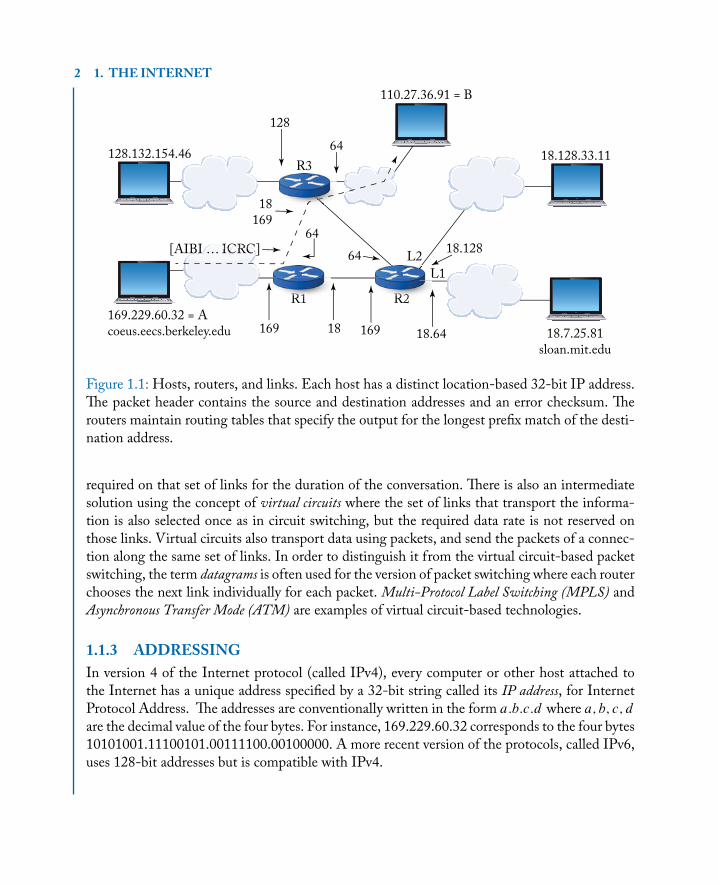
1.1.1 HOSTS, ROUTERS, LINKSThe Internet consists of hosts and routers attached to each other with links. The hosts are sourcesor sinks of information. The name “hosts” indicates that these devices host the applicationsthat generate or use the information they exchange over the network. Hosts include computers,printers, servers, web cams, etc. The routers receive information and forward it to the next routeror host. A link transports bits between two routers or hosts. Links are either optical, wired(including cable), or wireless. Some links are more complex and involve switches, as we studylater. Figure 1.1 shows a few hosts and routers attached with links. The clouds represent othersets of routers and links.

1.1.2 PACKET SWITCHINGThe original motivation for the Internet was to build a network that would be robust againstattacks on some of its parts. The initial idea was that, should part of the network get disabled,routers would reroute information automatically along alternate paths. This flexible routing isbased on packet switching. Using packet switching, the network transports bits grouped in packets.A packet is a string of bits arranged according to a specified format. An Internet packet containsits source and destination addresses. Figure 1.1 shows a packet with its source address A anddestination address B . Switching refers to the selection of the set of links that a packet followsfrom its source to its destination. Packet switching means that the routers make this selectionindividually for each packet. In contrast, the telephone network uses circuit switching where itselects the set of links only once for a complete telephone conversation and reserves the data rate

2 1. THE INTERNET

128

169 16918

64

64

64

18169

18.128

18.64

18.128.33.11R3

R1 R2

L1

L2

18.7.25.81sloan.mit.edu

R1R1R1R1R1R1R1R1R1R1R1R1R1 R2R2R2R2R2R2R2R2R2R2R2R2R2

L1L1

128.132.154.46

110.27.36.91 = B

169.229.60.32 = Acoeus.eecs.berkeley.edu

[AIBI … ICRC]

Figure 1.1: Hosts, routers, and links. Each host has a distinct location-based 32-bit IP address.The packet header contains the source and destination addresses and an error checksum. Therouters maintain routing tables that specify the output for the longest prefix match of the desti-nation address.

required on that set of links for the duration of the conversation. There is also an intermediatesolution using the concept of virtual circuits where the set of links that transport the informa-tion is also selected once as in circuit switching, but the required data rate is not reserved onthose links. Virtual circuits also transport data using packets, and send the packets of a connec-tion along the same set of links. In order to distinguish it from the virtual circuit-based packetswitching, the term datagrams is often used for the version of packet switching where each routerchooses the next link individually for each packet. Multi-Protocol Label Switching (MPLS) andAsynchronous Transfer Mode (ATM) are examples of virtual circuit-based technologies.

1.1.3 ADDRESSINGIn version 4 of the Internet protocol (called IPv4), every computer or other host attached tothe Internet has a unique address specified by a 32-bit string called its IP address, for InternetProtocol Address. The addresses are conventionally written in the form a:b:c:d where a; b; c; dare the decimal value of the four bytes. For instance, 169.229.60.32 corresponds to the four bytes10101001.11100101.00111100.00100000. A more recent version of the protocols, called IPv6,uses 128-bit addresses but is compatible with IPv4.

1.1. BASIC OPERATIONS 3

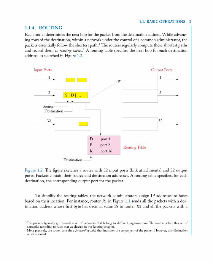
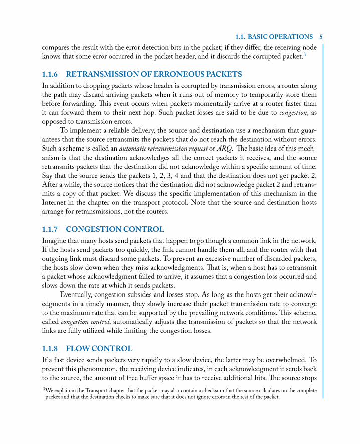
1.1.4 ROUTINGEach router determines the next hop for the packet from the destination address. While advanc-ing toward the destination, within a network under the control of a common administrator, thepackets essentially follow the shortest path.1 The routers regularly compute these shortest pathsand record them as routing tables.2 A routing table specifies the next hop for each destinationaddress, as sketched in Figure 1.2.

S | D | …

D port 1

F port 2

K port 16Routing Table

Input Ports Output Ports

1

2

32

1

2

32

SourceDestination

Destination

Figure 1.2: The figure sketches a router with 32 input ports (link attachments) and 32 outputports. Packets contain their source and destination addresses. A routing table specifies, for eachdestination, the corresponding output port for the packet.

To simplify the routing tables, the network administrators assign IP addresses to hostsbased on their location. For instance, router R1 in Figure 1.1 sends all the packets with a des-tination address whose first byte has decimal value 18 to router R2 and all the packets with a

1The packets typically go through a set of networks that belong to different organizations. The routers select this set ofnetworks according to rules that we discuss in the Routing chapter.

2More precisely, the router consults a forwarding table that indicates the output port of the packet. However, this distinctionis not essential.

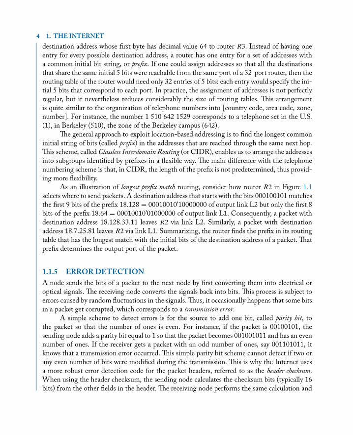
4 1. THE INTERNETdestination address whose first byte has decimal value 64 to router R3. Instead of having oneentry for every possible destination address, a router has one entry for a set of addresses witha common initial bit string, or prefix. If one could assign addresses so that all the destinationsthat share the same initial 5 bits were reachable from the same port of a 32-port router, then therouting table of the router would need only 32 entries of 5 bits: each entry would specify the ini-tial 5 bits that correspond to each port. In practice, the assignment of addresses is not perfectlyregular, but it nevertheless reduces considerably the size of routing tables. This arrangementis quite similar to the organization of telephone numbers into [country code, area code, zone,number]. For instance, the number 1 510 642 1529 corresponds to a telephone set in the U.S.(1), in Berkeley (510), the zone of the Berkeley campus (642).

The general approach to exploit location-based addressing is to find the longest commoninitial string of bits (called prefix) in the addresses that are reached through the same next hop.This scheme, called Classless Interdomain Routing (or CIDR), enables us to arrange the addressesinto subgroups identified by prefixes in a flexible way. The main difference with the telephonenumbering scheme is that, in CIDR, the length of the prefix is not predetermined, thus provid-ing more flexibility.

As an illustration of longest prefix match routing, consider how router R2 in Figure 1.1selects where to send packets. A destination address that starts with the bits 000100101 matchesthe first 9 bits of the prefix 18.128 D 00010010’10000000 of output link L2 but only the first 8bits of the prefix 18.64 D 00010010’01000000 of output link L1. Consequently, a packet withdestination address 18.128.33.11 leaves R2 via link L2. Similarly, a packet with destinationaddress 18.7.25.81 leaves R2 via link L1. Summarizing, the router finds the prefix in its routingtable that has the longest match with the initial bits of the destination address of a packet. Thatprefix determines the output port of the packet.

1.1.5 ERROR DETECTIONA node sends the bits of a packet to the next node by first converting them into electrical oroptical signals. The receiving node converts the signals back into bits. This process is subject toerrors caused by random fluctuations in the signals. Thus, it occasionally happens that some bitsin a packet get corrupted, which corresponds to a transmission error.

A simple scheme to detect errors is for the source to add one bit, called parity bit, tothe packet so that the number of ones is even. For instance, if the packet is 00100101, thesending node adds a parity bit equal to 1 so that the packet becomes 001001011 and has an evennumber of ones. If the receiver gets a packet with an odd number of ones, say 001101011, itknows that a transmission error occurred. This simple parity bit scheme cannot detect if two orany even number of bits were modified during the transmission. This is why the Internet usesa more robust error detection code for the packet headers, referred to as the header checksum.When using the header checksum, the sending node calculates the checksum bits (typically 16bits) from the other fields in the header. The receiving node performs the same calculation and

1.1. BASIC OPERATIONS 5compares the result with the error detection bits in the packet; if they differ, the receiving nodeknows that some error occurred in the packet header, and it discards the corrupted packet.3

1.1.6 RETRANSMISSION OF ERRONEOUS PACKETSIn addition to dropping packets whose header is corrupted by transmission errors, a router alongthe path may discard arriving packets when it runs out of memory to temporarily store thembefore forwarding. This event occurs when packets momentarily arrive at a router faster thanit can forward them to their next hop. Such packet losses are said to be due to congestion, asopposed to transmission errors.

To implement a reliable delivery, the source and destination use a mechanism that guar-antees that the source retransmits the packets that do not reach the destination without errors.Such a scheme is called an automatic retransmission request or ARQ. The basic idea of this mech-anism is that the destination acknowledges all the correct packets it receives, and the sourceretransmits packets that the destination did not acknowledge within a specific amount of time.Say that the source sends the packets 1, 2, 3, 4 and that the destination does not get packet 2.After a while, the source notices that the destination did not acknowledge packet 2 and retrans-mits a copy of that packet. We discuss the specific implementation of this mechanism in theInternet in the chapter on the transport protocol. Note that the source and destination hostsarrange for retransmissions, not the routers.

1.1.7 CONGESTION CONTROLImagine that many hosts send packets that happen to go though a common link in the network.If the hosts send packets too quickly, the link cannot handle them all, and the router with thatoutgoing link must discard some packets. To prevent an excessive number of discarded packets,the hosts slow down when they miss acknowledgments. That is, when a host has to retransmita packet whose acknowledgment failed to arrive, it assumes that a congestion loss occurred andslows down the rate at which it sends packets.

Eventually, congestion subsides and losses stop. As long as the hosts get their acknowl-edgments in a timely manner, they slowly increase their packet transmission rate to convergeto the maximum rate that can be supported by the prevailing network conditions. This scheme,called congestion control, automatically adjusts the transmission of packets so that the networklinks are fully utilized while limiting the congestion losses.

1.1.8 FLOW CONTROLIf a fast device sends packets very rapidly to a slow device, the latter may be overwhelmed. Toprevent this phenomenon, the receiving device indicates, in each acknowledgment it sends backto the source, the amount of free buffer space it has to receive additional bits. The source stops3We explain in the Transport chapter that the packet may also contain a checksum that the source calculates on the completepacket and that the destination checks to make sure that it does not ignore errors in the rest of the packet.

6 1. THE INTERNETtransmitting when this available space is not larger than the number of bits the source has alreadysent and the receiver has not yet acknowledged.

The source combines the flow control scheme with the congestion control scheme discussedearlier. Note that flow control prevents overflowing the destination buffer, whereas congestioncontrol prevents overflowing router buffers.

1.2 DNS, HTTP, AND WWW1.2.1 DNSThe hosts attached to the Internet have a name in addition to an IP address. The names areeasier to remember (e.g., google.com). To send packets to a host, the source needs to know theIP address of that host. The Internet has an automatic directory service called the Domain NameService, or DNS, that translates the name into an IP address. DNS is a distributed directory ser-vice. The Internet is decomposed into zones, and a separate DNS server maintains the addressesof the hosts in each zone. For instance, the department of EECS at Berkeley maintains thedirectory server for the hosts in the eecs.berkeley.edu zone of the network. The DNS server forthat zone answers requests for the IP address of hosts in that zone. Consequently, if one adds ahost on the network of our department, one needs to update only that DNS server.

1.2.2 HTTP AND WWWTheWorldWideWeb is arranged as a collection of hyperlinked resources such as web pages, videostreams, and music files. The resources are identified by a Uniform Resource Locator or URL thatspecifies a computer and a file in that computer together with the protocol that should deliverthe file.

For instance, the URL http://www.eecs.berkeley.edu/~wlr.html specifies a homepage in a computer with name www.eecs.berkeley.edu and the protocol HTTP.

HTTP, the Hyper Text Transfer Protocol, specifies the request/response rules for gettingthe file from a server to a client. Essentially, the protocol sets up a connection between the serverand the client, then requests the specific file, and finally closes the connection when the transferis complete.

1.3 SUMMARY• The Internet consists of hosts that send and/or receive information, routers, and links.

• Each host has a 32-bit IP address (in IPv4; 128-bit in IPv6) and a name. DNS is a dis-tributed directory service that translates the name into an IP address.

• The hosts arrange the information into packets that are groups of bits with a specifiedformat. A packet includes its source and destination addresses and error detection bits.

http://www.eecs.berkeley.edu/~wlr.html

1.4. PROBLEMS 7• The routers calculate the shortest paths (essentially) to destinations and store them in rout-

ing tables. The IP addresses are based on the location of the hosts to reduce the size ofrouting tables using longest prefix match.

• A source adjusts its transmissions to avoid overflowing the destination buffer (flow control)and the buffers of the routers (congestion control).

• Hosts remedy transmission and congestion losses by using acknowledgments, timeouts,and retransmissions.

1.4 PROBLEMSP1.1 How many hosts can one have on the Internet if each one needs a distinct IPv4 address?

P1.2 If the addresses were allocated arbitrarily, how many entries should a routing table have?

P1.3 Imagine that all routers have 16 ports. In the best allocation of addresses, what is the sizeof the routing table required in each router?

P1.4 Assume that a host A in Berkeley sends a stream of packets to a host B in Boston. Assumealso that all links operate at 100 Mbps and that it takes 130 ms for the first acknowledg-ment to come back after A sends the first packet. Say that A sends one packet of 1 KByteand then waits for an acknowledgment before sending the next packet, and so on. Whatis the long-term average bit rate of the connection? Assume now that A sends N packetsbefore it waits for the first acknowledgment, and that A sends the next packet every timean acknowledgment is received. Express the long-term average bit rate of the connectionas a function ofN . [Note: 1 Mbps D 106 bits per second; 1 ms D 1 millisecond D 10�3 s.]

P1.5 Assume that a host A in Berkeley sends 1-KByte packets with a bit rate of 100 Mbps to ahost B in Boston. However, B reads the bits only at 1 Mbps. Assume also that the devicein Boston uses a buffer that can store 10 packets. Explore the flow control mechanism andprovide a time line of the transmissions.

1.5 REFERENCESPacket switching was independently invented in the early 1960s by Paul Baran [14], DonaldDavies, and Leonard Kleinrock who observed, in his MIT thesis [56], that packet-switchednetworks can be analyzed using queuing theory. Bob Kahn and Vint Cerf invented the basicstructure of TCP/IP in 1973 [52].The congestion control of TCPwas corrected by Van Jacobsonin 1988 [49], partly motivated by the analysis by Chiu and Jain [25] and [26] and also by thestability of linear systems. Paul Mockapetris invented DNS in 1983. CIDR is described in [34].Tim Berners-Lee invented the WWW in 1989. See [40] for a discussion of the AutonomousSystems.

9

C H A P T E R 2

PrinciplesIn networking, connectivity is the name of the game. The Internet connects a few billion com-puters across the world, plus associated devices such as printers, servers, and web cams. Withthe development of the Internet of Things, hundreds of billions of devices will soon be con-nected via the Internet. By “connect,” we mean that the Internet enables these hosts to transferfiles or bit streams among each other. To reduce cost, all these hosts share communication links.For instance, many users in the same neighborhood may share a coaxial cable to connect to theInternet; many communications share the same optical fibers. With this sharing, the networkcost per user is relatively small.

To accommodate its rapid growth, the Internet is organized in a hierarchical way andadding hosts to it only requires local modifications. Moreover, the network is independent ofthe applications that it supports. That is, only the hosts need the application software. For in-stance, the Internet supports video conferences even though its protocols were designed beforevideo conferences existed. In addition, the Internet is compatible with new technologies such aswireless communications or improvements in optical links.

We comment on these important features in this chapter. In addition, we introduce somemetrics that quantify the performance characteristics of a network.

2.1 SHARING

Imagine designing a network to interconnect a few billion devices such as computers, smartphones, thermostats, etc. It is obviously not feasible to connect each pair of devices with a ded-icated link. Instead, one attaches devices that are close to each other with a local network. Onethen attaches local networks together with an access network. One attaches the access networkstogether in a regional network. Finally, one connects the regional networks together via one ormore backbone networks that go across the country, as shown in Figure 2.1.

This arrangement reduces considerably the total length of wires needed to attach the de-vices together, when compared with pairwise links. Many devices share links and routers. Forinstance, all the devices in the leftmost access network of the figure share the link L as theysend information to devices in another access network. What makes this sharing possible is thefact that the devices do not transmit all the time. Accordingly, only a small fraction of devicesare active and share the network links and routers, which reduces the investment required perdevice.

10 2. PRINCIPLES

Backbone

Regional

Access

Local

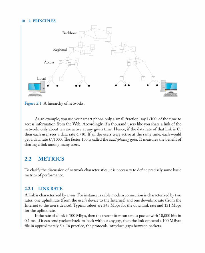
Figure 2.1: A hierarchy of networks.

As an example, you use your smart phone only a small fraction, say 1=100, of the time toaccess information from the Web. Accordingly, if a thousand users like you share a link of thenetwork, only about ten are active at any given time. Hence, if the data rate of that link is C ,then each user sees a data rate C=10. If all the users were active at the same time, each wouldget a data rate C=1000. The factor 100 is called the multiplexing gain. It measures the benefit ofsharing a link among many users.

2.2 METRICS

To clarify the discussion of network characteristics, it is necessary to define precisely some basicmetrics of performance.

2.2.1 LINK RATEA link is characterized by a rate. For instance, a cable modem connection is characterized by tworates: one uplink rate (from the user’s device to the Internet) and one downlink rate (from theInternet to the user’s device). Typical values are 343 Mbps for the downlink rate and 131 Mbpsfor the uplink rate.

If the rate of a link is 100 Mbps, then the transmitter can send a packet with 10,000 bits in0.1 ms. If it can send packets back-to-back without any gap, then the link can send a 100 MBytefile in approximately 8 s. In practice, the protocols introduce gaps between packets.

2.2. METRICS 11A link that connects a user to the Internet is said to be broadband if its rate exceeds 25Mbps

downlink and 4 Mbps uplink. (This is the value defined by the Federal Communication Com-mission in 2015.) Otherwise, one says that the link is narrowband.

2.2.2 LINK BANDWIDTH AND CAPACITYA signal of the form V.t/ D A sin.2�f0t/ makes f0 cycles per second. We say that its frequencyis f0 Hz. Here, Hz stands for Hertz and means one cycle per second. For instance, V.t/may bethe voltage at time t as measured across the two terminals of a telephone line. The physics of atransmission line limits the set of frequencies of signals that it transports. The bandwidth of acommunication link measures the width of that range of frequencies. For instance, if a telephoneline can transmit signals over a range of frequencies from 300 Hz to 1 MHz ( = 106 Hz), wesay that its bandwidth is about 1 MHz.

The rate of a link is related to its bandwidth. Intuitively, if a link has a large bandwidth, itcan carry voltages that change very quickly and it should be able to carry many bits per seconds,as different bits are represented by different voltage values. The maximum rate of a link dependsalso on the amount of noise on the link. If the link is very noisy, the transmitter should send bitsmore slowly. This is similar to having to articulate more clearly when talking in a noisy room.

An elegant formula due to Claude Shannon indicates the relationship between the maxi-mum reliable link rate C , also called the Shannon Capacity of the link, its bandwidth W , and thenoise. That formula is

C D W log2.1C SNR/:

In this expression, SNR, the signal-to-noise ratio, is the ratio of the power of the signal at thereceiver divided by the power of the noise, also at the receiver. For instance, if SNR D 106 �

220 andW D 1MHz, then we find thatC D 106 log2.1C 106/bps � 106 log2.220/bps D 106 �

20 bps D 20 Mbps. This value is the theoretical limit that could be achieved, using the bestpossible technique for representing bits by signals and the best possible method to avoid orcorrect errors. An actual link never quite achieves the theoretical limit, but it may come close.

The formula confirms the intuitive fact that if a link is longer, then its capacity is smaller.Indeed, the power of the signal at the receiver decreases with the length of the link (for a fixedtransmitter power). For instance, a Digital Subscriber Loop (DSL) link over a telephone line thatis very long has a smaller rate than a shorter line. The formula also explains why a coaxial cablecan have larger rate than a telephone line if one knows that the bandwidth of the former is wider.

In a more subtle way, the formula shows that if the transmitter has a given power, it shouldallocate more power to the frequencies within its spectrum that are less noisy. Over a cello, onehears a soprano better than a basso profundo. A DSL transmitter divides its power into smallfrequency bands, and it allocates more power to the less noisy portions of the spectrum.

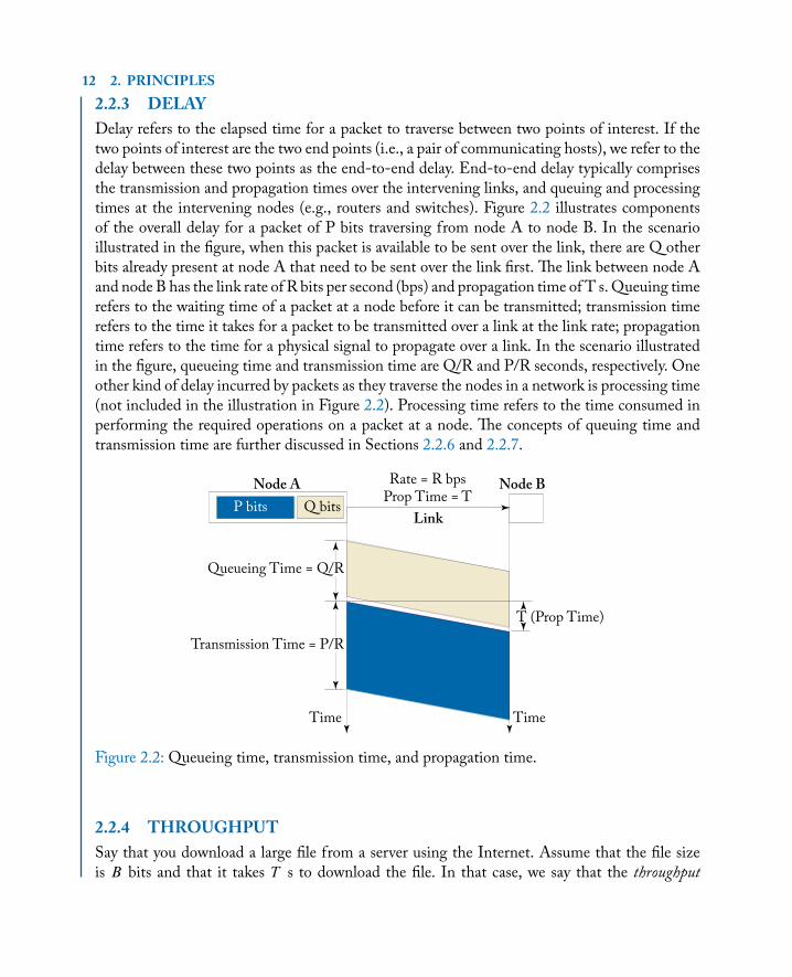
12 2. PRINCIPLES2.2.3 DELAYDelay refers to the elapsed time for a packet to traverse between two points of interest. If thetwo points of interest are the two end points (i.e., a pair of communicating hosts), we refer to thedelay between these two points as the end-to-end delay. End-to-end delay typically comprisesthe transmission and propagation times over the intervening links, and queuing and processingtimes at the intervening nodes (e.g., routers and switches). Figure 2.2 illustrates componentsof the overall delay for a packet of P bits traversing from node A to node B. In the scenarioillustrated in the figure, when this packet is available to be sent over the link, there are Q otherbits already present at node A that need to be sent over the link first. The link between node Aand node B has the link rate of R bits per second (bps) and propagation time of T s.Queuing timerefers to the waiting time of a packet at a node before it can be transmitted; transmission timerefers to the time it takes for a packet to be transmitted over a link at the link rate; propagationtime refers to the time for a physical signal to propagate over a link. In the scenario illustratedin the figure, queueing time and transmission time are Q/R and P/R seconds, respectively. Oneother kind of delay incurred by packets as they traverse the nodes in a network is processing time(not included in the illustration in Figure 2.2). Processing time refers to the time consumed inperforming the required operations on a packet at a node. The concepts of queuing time andtransmission time are further discussed in Sections 2.2.6 and 2.2.7.

Node A Node B

LinkP bits Q bits

Queueing Time = Q/R

Transmission Time = P/R

T (Prop Time)

Time

Rate = R bpsProp Time = T

Time

Figure 2.2: Queueing time, transmission time, and propagation time.

2.2.4 THROUGHPUTSay that you download a large file from a server using the Internet. Assume that the file sizeis B bits and that it takes T s to download the file. In that case, we say that the throughput

2.2. METRICS 13of the transfer is B=T bps. For instance, you may download an MP4 video file of 3 GBytes =24 Gbits in 4 min, i.e., 240 s. The throughput is then 24 Gbits/240 s D 0.1 Gbps or 100 Mbps.(For convenience, we approximate 1 GByte by 109 bytes even though it is actually 230 D

1,073,741,824 bytes. Recall also that one defines 1 Mbps = 106 bps and 1 Kbps D 103 bps.)The link rate is not the same as the throughput. For instance, in the example above, your

video download had a throughput of 100 Mbps. You might have been using a cable modem witha downlink rate of 343 Mbps. The difference comes from the fact that the download correspondsto a sequence of packets and there are gaps between the packets.

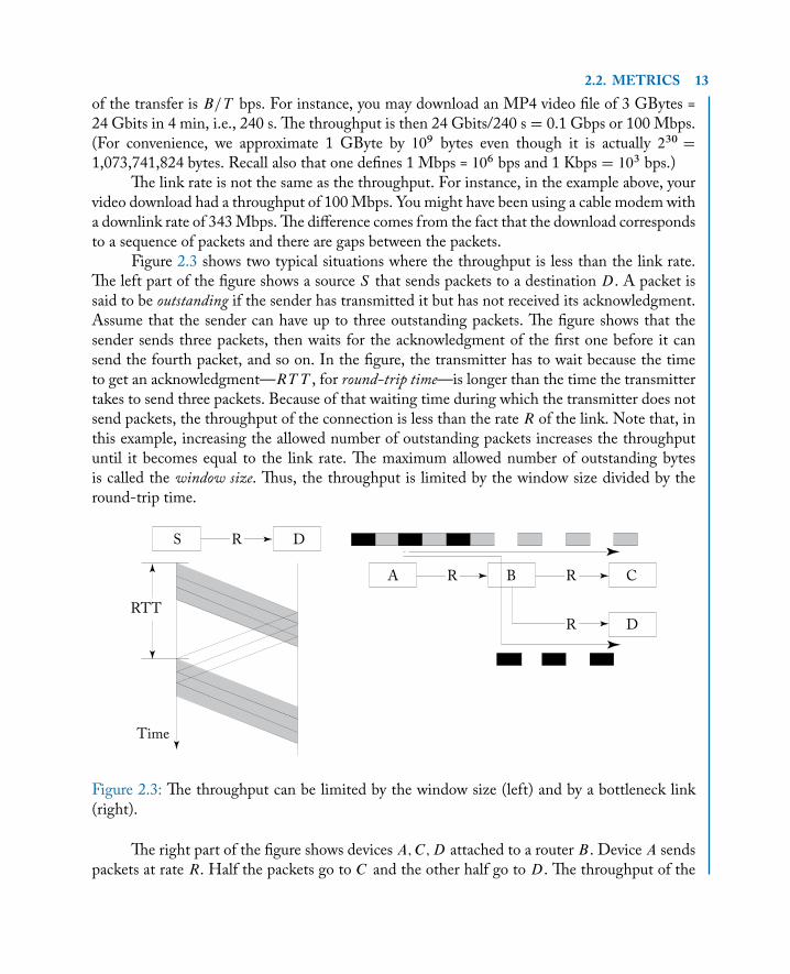
Figure 2.3 shows two typical situations where the throughput is less than the link rate.The left part of the figure shows a source S that sends packets to a destination D. A packet issaid to be outstanding if the sender has transmitted it but has not received its acknowledgment.Assume that the sender can have up to three outstanding packets. The figure shows that thesender sends three packets, then waits for the acknowledgment of the first one before it cansend the fourth packet, and so on. In the figure, the transmitter has to wait because the timeto get an acknowledgment—RT T , for round-trip time—is longer than the time the transmittertakes to send three packets. Because of that waiting time during which the transmitter does notsend packets, the throughput of the connection is less than the rate R of the link. Note that, inthis example, increasing the allowed number of outstanding packets increases the throughputuntil it becomes equal to the link rate. The maximum allowed number of outstanding bytesis called the window size. Thus, the throughput is limited by the window size divided by theround-trip time.

A B C

D

S DR

R R

R

Time

RTT

Figure 2.3: The throughput can be limited by the window size (left) and by a bottleneck link(right).

The right part of the figure shows devices A;C;D attached to a router B . Device A sendspackets at rate R. Half the packets go to C and the other half go to D. The throughput of the

14 2. PRINCIPLESconnection fromA to C isR=2whereR is the rate of the links. Thus, the two connections (fromA to C and from A to D) share the rate R of the link from A to B . This link is the bottleneck ofthe system: it is the rate of that link that limits the throughput of the connections. Increasingthe rate of that link would enable to increase the throughput of the connections.

2.2.5 DELAY JITTERThe successive packets that a source sends to a destination do not face exactly the same delayacross the network. One packet may reach the destination in 50 ms whereas another one maytake 120 ms. These fluctuations in delay are due to the variable amount of congestion in therouters. A packet may arrive at a router that has already many other packets to transmit. Anotherpacket may be lucky and have rarely to wait behind other packets. One defines the delay jitter ofa connection as the difference between the longest and shortest delivery time among the packetsof that connection. For instance, if the delivery times of the packets of a connection range from50 ms to 120 ms, the delay jitter of that connection is 70 ms.

Many applications such as streaming audio or video and voice-over-IP are sensitive todelays. Those applications generate a sequence of packets that the network delivers to the des-tination for playback. If the delay jitter of the connection is J , the destination should store thefirst packet that arrives for at least J seconds before playing it back, so that the destination neverruns out of packets to play back. In practice, the value of the delay jitter is not known in ad-vance. Typically, a streaming application stores the packets for T s, say T D 4, before startingto play them back. If the playback buffer gets empty, the application increases the value of T ,and it buffers packets for T s before playing them back. The initial value of T and the rule forincreasing T depend on the application. A small value of T is important for interactive applica-tions such as voice over IP or video conferences; it is less critical for one-way streaming such asInternet radio, IPTV, or YouTube.

2.2.6 M/M/1 QUEUETo appreciate effects such as congestion, jitter, and multiplexing, it is convenient to recall a basicresult about delays in a queue. Imagine that customers arrive at a cash register and queue upuntil they can be served. Assume that one customer arrives in the next second with probability�, independently of when previous customers arrived. Assume also that the cashier completesthe service of a customer in the next second with probability �, independently of how long hehas been serving that customer and of how long it took to serve the previous customers. Thatis, � customers arrive per second, on average, and the cashier serves � customers per second, onaverage, when there are customers to be served.Note that the average service time per customer is1=� s since the cashier can serve � customers per second, on average. One defines the utilizationof the system as the ratio � D �=�. Thus, the utilization is 80% if the arrival rate is equal to 80%of the service rate.

2.2. METRICS 15Such a system is called an M/M/1 queue. In this notation, the first M indicates that the

arrival process is memoryless: the next arrival occurs with probability � in the next second, nomatter how long it has been since the previous arrival. The second M indicates that the serviceis also memoryless. The 1 in the notation indicates that there is only one server (the cashier).

Assume that � < � so that the cashier can keep up with the arriving customers. The basicresult is that the average time T that a customer spends waiting in line or being served is givenby

T D1

� � �:

If � is very small, then the queue is almost always empty when a customer arrives. In that case,the average time T is 1=� and is equal to the average time the cashier spends serving a customer.Consequently, for any given � < �, the difference T � 1=� is the average queuing time that acustomer waits behind other customers before getting to the cashier.

Another useful result is that the average number L of customers in line or with the serveris given by

L D�

� � �:

Note that T and L grow without bound as � increases and approaches �.To apply these results to communication systems, one considers that the customers are

packets, the cashier is a transmitter, and the waiting line is a buffer attached to the transmitter.The average packet service time 1=� (in seconds) is the average packet length (in bits) dividedby the link rate (in bps). Equivalently, the service rate � is the link rate divided by the averagelength of a packet. Consider a computer that generates � packets per second and that thesepackets arrive at a link that can send � packets per second. The formulas above provide theaverage delay T per packet and the average number L of packets stored in the link’s transmitterqueue.

For concreteness, say that the line rate is 10 Mbps, that the packets are 1 Kbyte long, onaverage, and that 1,000 packets arrive at the transmitter per second, also on average. In this case,one finds that

� D107

8 � 103D 1,250 packets per second:

Consequently,

T D1

� � �D

1

1,250 � 1,000 D 4ms and L D�

� � �D

1,0001,250 � 1,000 D 4:

Thus, an average packet transmission time is 1=� D 0.8ms, the average delay through the systemis 4 ms, and four packets are in the buffer, on average. A typical packet that arrives at the bufferfinds 4 other packets already there; that packet waits for the 4 transmission times of those packetsthen for its own transmission time before it is out of the system. The average delay corresponds

16 2. PRINCIPLESto 5 transmission times of 0.8 ms each, so that T D 4 ms. This delay T consists of the queuingtime 3.2 ms and one transmission time 0.8 ms.

Because of the randomness of the arrivals of packets and of the variability of the transmis-sion times, not all packets experience the same delay. With the M/M/1 model, it is, in principle,possible for a packet to arrive at the buffer when it contains a very large number of packets. How-ever, that is not very likely. One can show that about 5% of the packets experience a delay largerthan 12 ms and about 5% will face a delay less than 0.2 ms. Thus, most of the packets have adelay between 0.2 ms and 12 ms. One can then consider that the delay jitter is approximately12 ms, or three times the average delay through the buffer.

To appreciate the effect of congestion, assume now that the packets arrive at the rate of1,150 packets per second. One then finds that T D 10 ms and L D 11:5. In this situation, thetransmission time is still 0.8 ms but the average queuing time is equal to 11.5 transmission times,or 9.2 ms. The delay jitter for this system is now about 30 ms. Thus, the average packet delayand the delay jitter increase quickly as the arrival rate of packets � approaches the transmissionrate �.

Now imagine that N computers share a link that can send N� packets per second. In thiscase, replacing � by N� and � by N� in the previous formulas, we find that the average delayis now T=N and that the average number of packets is still L. Thus, by sharing a faster link,the packets face a smaller delay. This effect, which is not too surprising if we notice that thetransmission time of each packet is now much smaller, is another benefit of having computersshare fast links through switches instead of having slower dedicated links.

Summarizing, the M/M/1 model enables us to estimate the delay and backlog at a trans-mission line. The average transmission time (in seconds) is the average packet length (in bits)divided by the link rate (in bps). For a moderate utilization � (say � � 80%), the average delayis a small multiple of the average transmission time (say 3–5 times). Also, the delay jitter can beestimated as about 3 times the average delay through the buffer.

2.2.7 LITTLE’S RESULTAnother basic result helps us understand some important aspects of networks: Little’s Result,discovered by John D. C. Little in 1961. Imagine a system where packets arrive with an averagerate of � packets per second. Designate by L the average number of packets in the system andby W the average time that a packet spends in the system. Then, under very weak assumptionson the arrivals and processing of the packets, the following relation holds:

L D �W:

Note that this relation, calledLittle’s Result, holds for theM/M/1 queue, as the formulas indicate.However, this result holds much more generally.

To understand Little’s Result, one can argue as follows. Imagine that a packet pays onedollar per second it spends in the system. Accordingly, the average amount that each packet pays

2.2. METRICS 17is W dollars. Since packets go through the system at rate �, the system gets paid at the averagerate of �W per second. Now, this average rate must be equal to the average number L of packetsin the system since they each pay at the rate of one dollar per second. Hence L D �W .

As an illustration, say that 1 billion users send 10 MBytes per day each via the Internet,on average. Assume also that each packet spends 0.4 s in the Internet, on average. The averagenumber of bits in transit on the Internet is then L where

L D �W D

�109

�8 � 107

24 � 3; 600bps

�� 0:4 s � 3:7 � 1011 bits � 43Gbytes:

Some of these bits are in transit in the fibers, the others are mostly in the routers.As another example, let us try to estimate how many bits are stored in a fiber. Consider

a fiber that transmits bits at the rate of 2.4 Gbps and the fiber is used at 20% of its capacity.Assume that the fiber is 100 km long. The propagation time of light in a fiber is about 5 �sper km. This is equal to the propagation time in a vacuum multiplied by the refractive indexof the fiber. Thus, each bit spends a time W in the fiber where W D 5�s � 100 D 5 � 10�4 s.The average arrival rate of bits in the fiber is � D 0:2 � 2:4 Gbps D 0:48 � 109 bps. By Little’sResult, the average number of bits stored in the fiber is L where

L D �W D�0:48 � 109 bps

��5 � 10�4 s

�D 2:4 � 105 bits D 30Kbytes:

A router also stores bits. To estimate how many, consider a router with 16 input ports at1 Gbps. Assume the router is used at 10% of its capacity. Assume also each bit spends 5 ms inthe router. We find that the average arrival rate of bits is � D 0:1 � 16 � 109 bps. The averagedelay is W D 5 � 10�3 s. Consequently, the average number L of bits in the router is

L D �W D�1:6 � 109 bps

��5 � 10�3 s

�D 8 � 106 bits D 1MByte:

2.2.8 FAIRNESSConsider two flows that share a link with rate 1 Mbps and assume that flow 1 values a givenrate twice as much as flow 2. How should they share the link capacity? One possibility is tomaximize the total value that the two flows derive from using the link. In this case, flow 1

should get the full capacity of the link, i.e., 1 Mbps, because it values it more than flow 2. Thisis called the max-sum allocation, or maximizing the social welfare. This solution does not seemfair to flow 2. Another possibility is to maximize the minimum utility of the two flows. If flow1 gets a rate x and flow 2 a rate 1 � x, the utility of flow 1 is A2x for some constant A and thatof flow 2 is A.1 � x/. To maximize the minimum, one chooses x so that A2x D A.1 � x/, i.e.,x D 1=3 and both flows get a utility equal to 2A=3. This is called the max-min allocation. Yetanother possibility is to maximize the product of the utilities 2Ax and A.1 � x/. In this case,x D 1=2 and the utility of flow 2 is equal to A whereas that of flow 2 is A=2. This allocationis called proportional fairness. Achieving fairness across a network is more challenging than thesimple example of the single link considered here. This can often lead to a trade-off between thenetwork efficiency and fairness. We will explore this issue further in the chapter on models.

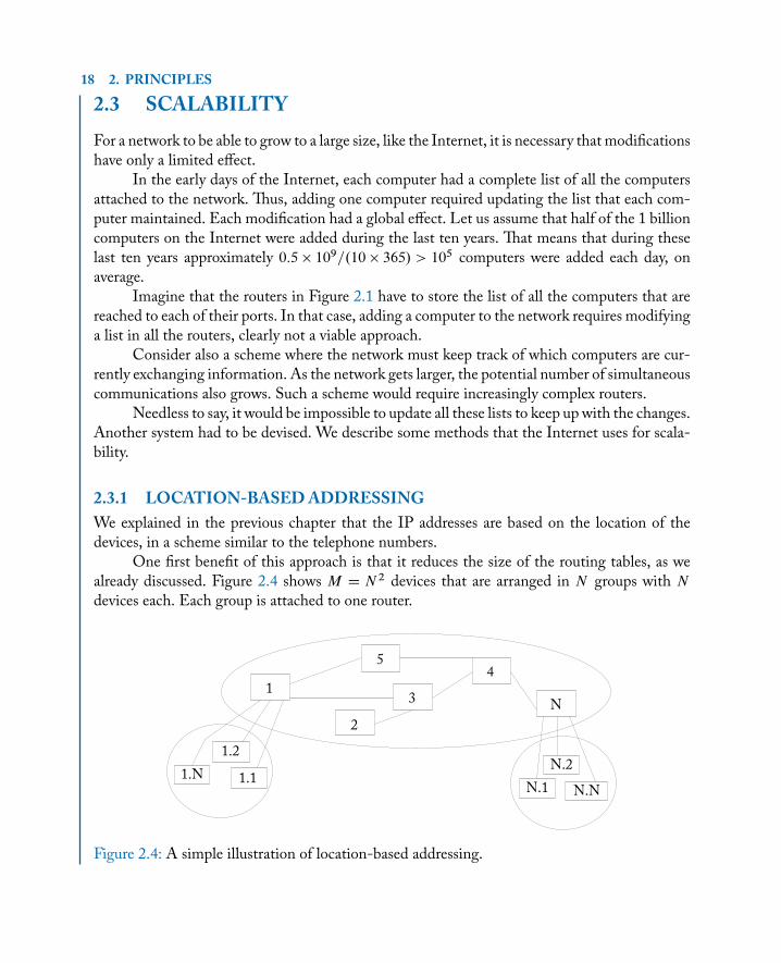
18 2. PRINCIPLES

2.3 SCALABILITYFor a network to be able to grow to a large size, like the Internet, it is necessary that modificationshave only a limited effect.

In the early days of the Internet, each computer had a complete list of all the computersattached to the network. Thus, adding one computer required updating the list that each com-puter maintained. Each modification had a global effect. Let us assume that half of the 1 billioncomputers on the Internet were added during the last ten years. That means that during theselast ten years approximately 0:5 � 109=.10 � 365/ > 105 computers were added each day, onaverage.

Imagine that the routers in Figure 2.1 have to store the list of all the computers that arereached to each of their ports. In that case, adding a computer to the network requires modifyinga list in all the routers, clearly not a viable approach.

Consider also a scheme where the network must keep track of which computers are cur-rently exchanging information. As the network gets larger, the potential number of simultaneouscommunications also grows. Such a scheme would require increasingly complex routers.

Needless to say, it would be impossible to update all these lists to keep up with the changes.Another system had to be devised. We describe some methods that the Internet uses for scala-bility.

2.3.1 LOCATION-BASED ADDRESSINGWe explained in the previous chapter that the IP addresses are based on the location of thedevices, in a scheme similar to the telephone numbers.

One first benefit of this approach is that it reduces the size of the routing tables, as wealready discussed. Figure 2.4 shows M D N 2 devices that are arranged in N groups with Ndevices each. Each group is attached to one router.

1

2

4

3N

5

1.1

1.2

1.N

N.N

N.2

N.1

Figure 2.4: A simple illustration of location-based addressing.

2.3. SCALABILITY 19In this arrangement, each router 1; : : : ; N needs one routing entry for each device in its

group plus one routing entry for each of the otherN � 1 routers. For instance, consider a packetthat goes from device 1.2 to device N.1. First, the packet goes from device 1.2 to router 1. Router1 has a routing entry that specifies the next hop toward routerN , say router 5. Similarly, router 5has a routing entry for the next hop, router 4, and so on. When the packet gets to router N , thelatter consults its routing table to find the next hop toward device N:1. Thus, each routing tablehas size N C .N � 1/ � 2

pM .

In contrast, we will explain that the Ethernet network uses addresses that have no relationto the location of the computers. Accordingly, the Ethernet switches need to maintain a list ofthe computers attached to each of their ports. Such an approach works fine for a relatively smallnumber of computers, say a few thousands, but does not scale well beyond that. If the networkhasM devices, each routing table needsM entries.

Assume that one day most electric devices will be attached to the Internet, such as lightbulbs, coffee machines, door locks, curtain motors, cars, etc. What is a suitable way to select theaddresses for these devices?

2.3.2 TWO-LEVEL ROUTINGThe Internet uses a routing strategy that scales at the cost of a loss of optimality. The mechanism,whose details we discuss in the chapter on routing, groups nodes into domains.

Each domain uses a shortest-path algorithm where the length of a path is defined as thesum of the metrics of the links along the path. A faster link has a smaller metric than a slowerlink.

To calculate the shortest path between two nodes in a domain, the switches must exchangequite a bit of metric information. For instance, each node could make up a message with thelist of its neighbors and the metrics of the corresponding links. The nodes can then send thesemessages to each other. For a simple estimate of the necessary number of messages, say thatthere are N routers and that each router sends one message to each of the other N � 1 routers.Thus, each router originates approximately N messages. For simplicity, say that each messagegoes through some average number of hops, say 6, that does not depend onN . The total numberof messages that the N routers transmit is then about 6N 2, or about 6N messages per router.This number of messages becomes impractical when N is very large.

To reduce the complexity of the routing algorithms, the Internet groups the routers intodomains. It then essentially computes a shortest path across domains and each domain computesshortest paths inside itself. Say that there are N domains with N routers inside each domain.Each router participates in a shortest path algorithm for its domain, thus sending about 6Nmessages. In addition, one representative router in each domain participates in a routing algo-rithm across domains, also sending of the order of 6N messages. If the routing were done in onelevel, each router would transmit 6N 2 messages, on average, which is N times larger than whenusing two-level routing.

20 2. PRINCIPLESIn the chapter on routing, we explain another motivation for a two-level routing approach.

It is rooted in the fact that inter-routing may correspond to economic arrangements as the do-mains belong to different organizations.

2.3.3 BEST EFFORT SERVICEA crucial design choice of the Internet is that it does not guarantee any precise property ofthe packet delivery such as delay or throughput. Instead, the designers opted for simplicity anddecided that the Internet should provide a “best effort service,” which means that the networkshould try to deliver the packets as well as possible, whatever this means. This design philosophyis in complete contrast with that of the telephone network where precise bounds are specifiedfor the time to get a dial tone, to ring a called party, and for the delay of transmission of the voicesignal. For instance, voice conversation becomes very unpleasant if the one-way delay exceeds250 ms. Consequently, how can one hope to use the Internet for voice conversations if it cannotguarantee that the delay is less than 250 ms? Similarly, a good video requires a throughput of atleast 50 Kbps. How can one use the Internet for such applications? The approach of the Internetis that, as its technology improves, it will become able to support more and more demandingapplications. Applications adapt to the changing quality of the Internet services instead of theother way around.

2.3.4 END-TO-END PRINCIPLE AND STATELESS ROUTERSBest effort service makes it unnecessary for routers (or the network) to keep track of the num-ber or types of connections that are set up. Moreover, errors are corrected by the source anddestination that arrange for retransmissions. More generally, the guiding principle is that tasksshould not be performed by routers if they can be performed by the end devices. This is calledthe end-to-end principle.

Thus, the routers perform their tasks for individual packets. The router detects if a givenpacket is corrupted and discards it in that case. The router looks at the packet’s destination ad-dress to determine the output port.The router does not keep a copy of a packet for retransmissionin the event of a transmission or congestion loss on the next hop. The router does not keep trackof the connections, of their average bit rate or of any other requirement.

Accordingly, routers can be stateless: they consider one packet at a time and do not haveany information about connections. This feature simplifies the design of routers, improves ro-bustness, and makes the Internet scalable.

2.3.5 HIERARCHICAL NAMINGThe Internet uses an automated directory service called DNS (for Domain Name System). Thisservice translates the name of a computer into its address. For instance, when youwant to connectto the Google server, the service tells your web browser the address that corresponds to the namewww.google.com of the server.

Documents

Synthesis Lectures on Communication Networks