Synthesis and characterization of spin

frustrated Fe doped LiCrO2

A thesis submitted in partial fulfillment for award of degree in

Master in science

In

Physics

Ms. Aakanksha Sahu

Roll No-412ph2111

Academic year: 2012-2014

Under the guidance of

Dr. Anil K. Singh

Department of Physics and Astronomy

National Institute of Technology,

Rourkela-769008, Odisha, India .

[1]

Aakanksha Sahu

Roll no:- 412ph2111

Department of Physics and Astronomy

National Institute of Technology

Rourkela-769008

DECLARATION

I hereby declare that the work carried out me at Department of Physics, National Institute of

Technology, Rourkela. I further declare that to best of my knowledge the carried out

experimental work has not formed the basis for the award of any degree, diploma, or similar title

of any university or institution.

Date:

Place:

[2]

ACKNOWLEDGEMENT

First of all I would like to thank the Almighty who enabled me to write this

acknowledgement. I would like to express my sincere gratitude to my advisor, Dr. A. K. Singh

for giving me the opportunity to work on the exciting research area of condensed matter physics.

I deeply appreciate all the time and effort he spent discussing my projects and advising me every

now and then. Without his guidance I would have never reached to the completion.

I would also like to thank all other faculty members in the Department of Physics &

Astronomy, NIT Rourkela. Specially I would like to thank Professor E. V. Sampathkmaran, Tata

Institute of Fundamental Research (TIFR), Mumbai for magnetization measurement. Also, I owe

my sincere thanks to the lab members Mr. Soumya Ranjan Mohapatra and Mr. Binayak Sahu of

Department of Physics for their guidance. Lastly, I would like to express my heartfelt thanks to

my beloved parents for their blessing and my friends for their kind help and wishes for the

successful completion of this project.

[3]

Department of Physics and Astronomy,

National Institute of Technology Rourkela

Rourkela-769008, Odisha, India

CERTIFICATE

This is to certify that the thesis entitled “Synthesis and Characterization of spin frustrated Fe

doped LiCrO2” being submitted by Ms. AAKANKSHA SAHU in partial fulfilment of the

requirements for the award of the degree of Masters of Science in Physics at National Institute of

Technology, Rourkela is an authentic experimental work carried out by her under our

supervision. To the best of our knowledge, the experimental matter embodied in the thesis has

not been submitted to any other University/Institute for the award of any degree or diploma.

Date: Dr. Anil K. Singh

[4]

Abstract

LiCrO2 and Fe doped LiCrO2 are prepared by solid state reaction method using LiCO3, Cr2O3,

and Fe2O3. From XRD data analysis we could confirm the phase purity of all the samples;

LiCrO2, LiCr0.98Fe0.02O2, and LiCr0.95Fe0.05O2. All the three samples show dispersion in dielectric

constant (εr) and dielectric loss factor (tan δ) values. The dielectric constant as a function of

frequency at different bias voltage has also been studied. Magnetization measurement for LiCrO2

using a SQUID magnetometer in a constant magnetic field of 100 Oe under zero field cooled and

field cooled condition show the antiferromagnetic transition temperature, TN ~ 64 K. The UV

visible plot reveals the slightly increase in band gap due to doping.

[5]

CONTENTS

1. INTRODUCTION Page no

1.1Magnetism 6

1.2. Ferroelectric material 7

1.3. Ferromagnetic material 8

1.4. Ferro elastic material 8

2. SPIN FRUSTRATION 9

3. MULTIFERROIC

3.1. Classification 9

3.2. Magneto electric coupling 10

4. APPLICATION 11

5. MOTIVATION 12

6. CRYSTAL STRUCTURE 12 7. SAMPLE PREPARATION 13

8. CHARACTERISATION TECHNIQUES

8.1. X-ray diffraction 15

8.2. Impedance spectroscopy 16

8.3. FESEM and EDAX 17

8.4. UV visible 18

8.5. SQUID measurement 19

9. RESULTS AND DISCUSSION

9.1. XRD 20

9.2. FESEM 21

9.3. UV visible 22

9.4. Impedance spectroscopy 23

9.5. SQUID data of LiCrO2 24

10. CONCLUSION 25

12. FUCTURE WORK 25

11. REFERENCES 26

[6]

1. INTRODUCTION

Magnetic materials play a very important role in modern life as we know that vast

numbers of devices are employed in electromagnetic industry. Before the confinement of

quantum mechanics a logical classification of magnetic materials was based up on the response

of every material to the magnetic field [1]. In general, it is classified into three categories. They

are as follows:

1.1 TYPES OF MAGNETISM

1.1.1 DIAMAGNETISM

Material having no net magnetic moments is called diamagnetic having negative

susceptibility. It is the weak form of magnetism. It is induced by a change in orbital motion of

electron due to an applied magnetic field. Most of the superconductors shows diamagnetism.

Example- Copper, Gold, Bismuth, Water.

1.1.2 PARAMAGNETISM

Substance which are weakly attracted by magnetic field having net magnetic moments,

positive susceptibility, obey curie’s law in which susceptibility is inversely proposal to

temperature (χ = C/T ) are known as paramagnetic materials. Magnetic permeability is greater

than μ0. In this kind of materials, magnetic moments are randomly aligned but when magnetic

field is applied some of the moments align along the field direction. Paramagnetic material are

used to produce very low temperature by adiabatic demagnetization.

Example- Lithium, Cesium, Tantalum, Sodium.

1.1.3 FERROMAGNETISM

Ferromagnetic materials are strongly attracted by magnetic field. Due to having unpaired

electron net magnetic moment exist, shows positive susceptibility, obeys Curie Weiss law (χ =C/

(T-TC)). Temperature at which the exchange energy is greater than the thermal energy and

ferromagnetism occurs at that temperature is called Curie temperature (Tc). Exchange energy is

minimized when all electrons have same spin.

[7]

Now we shall discuss about ferroics. There are three types of ferroics.

1.2 FERROELECTRIC MATERIALS

Ferroelectric materials show spontaneous polarization even in the absence of an electric

field. Ions in absence of the field, the positive and negative center do not coincide as a result it

creates a dipole moment. Due to the variation of polarization with electric field, it creates a

closed loop called the hysteresis loop. The ferroelectric material changes to para electric material

after certain temperature Tc, i.e. transition temperature or Curie temperature. These types of

crystals are classified in 2 groups: (a) Order-disorder group where the ferroelectric transition

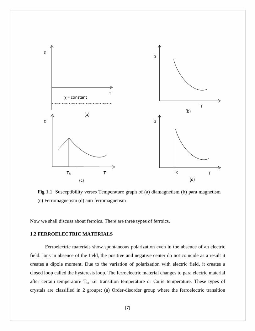
Fig 1.1: Susceptibility verses Temperature graph of (a) diamagnetism (b) para magnetism

(c) Ferromagnetism (d) anti ferromagnetism

(a)

(b)

(c)

(d)

χ = constant T

χ

(a)

χ

TN T

χ

(c)

TC T

χ

(d)

T

χ

(b) (a)

[8]

associates with individual ordering of ions. Example of this group is potassium dihydrogen

phosphate (b) Displacive group where the ferroelectric transition associates with the

displacement of a whole sublattice of ion of one type. The example of displacive group is

perovskite and ilmenite structure. And the examples of ferroelectric crystals are barium titanate,

Rochelle salt.

1.3 FERROMAGNETIC MATERIALS

Ferromagnetic materials possess spontaneous magnetization, i.e., magnetization exists

even in the absence of magnetic field. Large magnetization can be acquired by the material in

presence of even a weak external magnetic field. It also possesses a large value of susceptibility

but varies with field strength. This variation of magnetization with field strength creates

hysteresis curve. The example of these materials Fe, Ni, Co, Gd, Dy and some alloy like MnBi,

MnAs, CrO2.

1.4 FERROELASTIC MATERIALS

Ferroelastic materials possess spontaneous deformation and can be switched

hysteretically by an applied stress. Example- Nikel, Titanium.

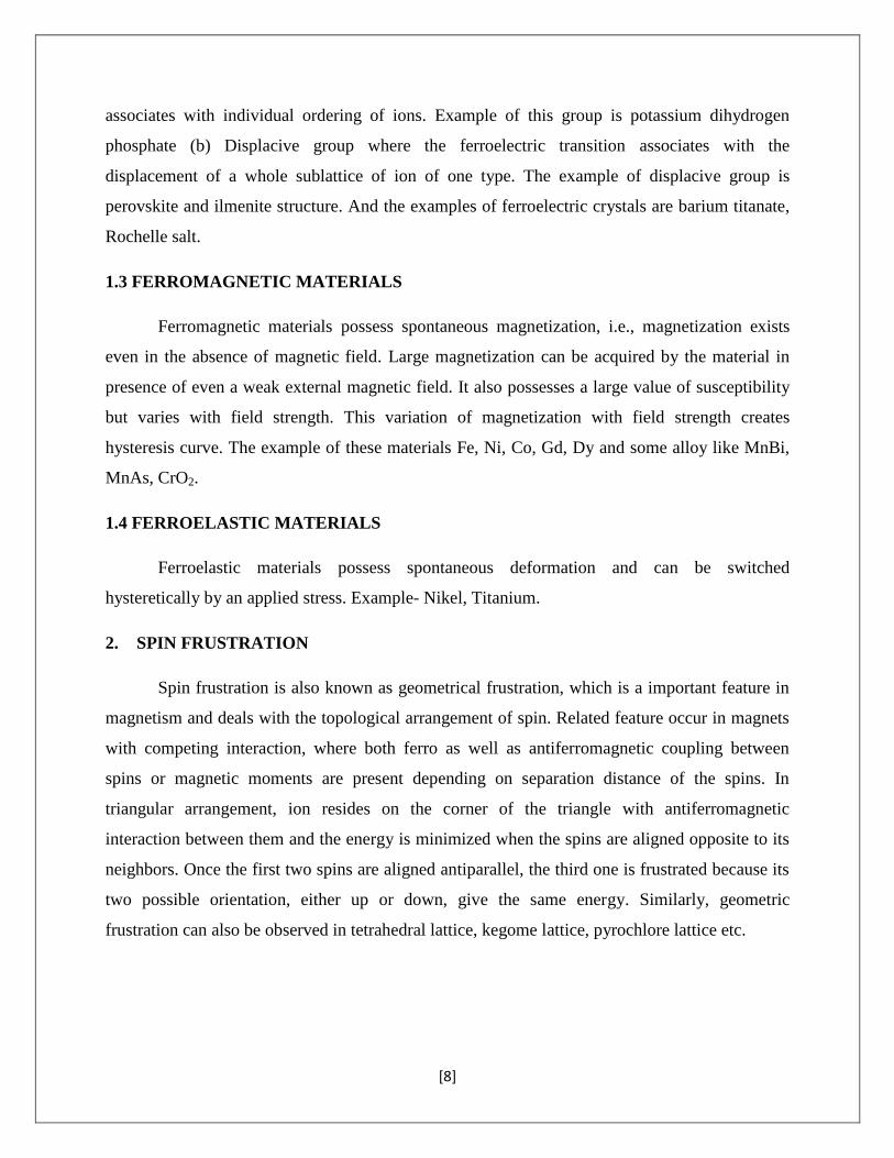
2. SPIN FRUSTRATION

Spin frustration is also known as geometrical frustration, which is a important feature in

magnetism and deals with the topological arrangement of spin. Related feature occur in magnets

with competing interaction, where both ferro as well as antiferromagnetic coupling between

spins or magnetic moments are present depending on separation distance of the spins. In

triangular arrangement, ion resides on the corner of the triangle with antiferromagnetic

interaction between them and the energy is minimized when the spins are aligned opposite to its

neighbors. Once the first two spins are aligned antiparallel, the third one is frustrated because its

two possible orientation, either up or down, give the same energy. Similarly, geometric

frustration can also be observed in tetrahedral lattice, kegome lattice, pyrochlore lattice etc.

[9]

3. MULTIFERROICS

Single phase material which simultaneously possess two or more primary ferroic

properties [2] are known as multiferroics. Boracites were probably the first known multiferroics.

At first in BiFeO3, discovery of a new class of multiferroics shows a large magneto electric

effect. A large magnetoelectric effect (a sudden change of electric polarization by the application

of magnetic fields) has been observed at the inception field in BiFeO3. It was established recently

in a class of materials known as ‘frustrated magnets’. There is Perovskites RMnO3, RMn2O5 (R:

rare earths), Ni3V2O8, CuFeO2, Spinel CoCr2O4, MnWO4.

3.1 CLASSIFICATION OF MULTIFERROICS

The magnetism in materials arises due to presence of localized electrons, mostly partially

filled d or f shells of transition metals or rare earth ions. But there are several different

microscopic sources of ferroelectricity [3] and accordingly we can categorize multiferroics in

two classes:

1) Type-I multiferroics

2) Type-II multiferroics

1) Type-I: In Type-I multiferroics, the cause of ferroelectricity and magnetism are from different

sources. In this class of materials, the ferroelectricity typically appears at higher temperatures

than magnetism and spontaneous polarisation P is often large (of the order 10-100 μC/cm2). Due

to this fact, the magnetism and ferroelectricity are independent of each other causing weak

coupling between them. e.g. BiFeO3, YMnO3, LuFe2O4 etc.

?

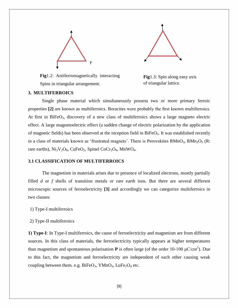
Fig1.2: Antiferromagnetically interacting

Spins in triangular arrangement.

spins in triangular arrangement

Fig1.3: Spin along easy axis

of triangular lattice.

[10]

2) Type–II: In Type-II multiferroics, magnetism causes ferroelectricity implying a strong

coupling between the two. In this class of materials, the value of ferroelectric polarization is

usually much smaller (~ 10-2

μC/cm2) and appear at very low temperature (below liquid N2

temperature) e.g. TbMnO3, TbMn2O5, Ni3V2O8 etc.

3.2 MAGNETOELECTRIC COUPLING (ME Coupling)

Magnetoelectric coupling has the potential to influence the magnetic state of matter

through the application of electric field. In the 1st single phase multiferroics combine both

electric and magnetic dipole moments in the same phase but only display low ordering

temperature. In 2nd

ferroelectric and ferromagnetic phases can be brought in to close contact so

that electric and magnetic dipoles coupled via the interface. In both the approaches, the

polarization can be a free electron charge near the surface. This phenomenon has been observed

in insulating material such as complex multiferroic oxides but not observed in bulk metallic

system because applied electric field is screened by a free electron charge near the surface.

The magneto electric effect in a single-phase crystal is described in landau theory, where

free energy is a function of electric field and magnetic field. It may be represented as an infinite

homogeneous and stress-free medium by F under the Einstein summation convention in S.I unit

as:

....2

1.

2

1

2

1

2

1),( 00 ijkkjiijkkjiijjiijjiijji EEHHHEHEHHEEHEF

Where, 0 = Permittivity of free space

µ0 = Permeability of free space

ij = Second rank tensor

µij = Relative permeability

βijk = Third rank tensor

The magneto electric (ME) effect is the phenomenon of inducing magnetic (electric) polarization

by applying an external electric (magnetic) field. The effects can be linear or non-linear with

[11]

respect to the external fields. In general, this effect depends on temperature. The effect can be

expressed in the following form.

...2

1

...2

1

0

kiijkijii

kjjkijjii

EEEM

HHHP

4. APPLICATION

Multiferroics have tremendous application in areas as diverse as data storage, sensing,

actuation and spintronics where electric field control of magnetic spin would consume

significantly less power than magnetic field control, which requires electric current to generate

magnetic fields [4, 5, & 6]. Magnetic field sensor is easier to measure small voltage at zero

applied current than small magnetization or small charges in resistivity [7]. Multistage memory

elements information are saved in both ferromagnetically and ferroelectric polarization. There is

a big hand of magnetoelectric material to improve behind magnetic field sensor.

5. MOTIVATION

In LiCrO2, lithium has very high storage capacities and chromium oxides have been

studied as potential cathode material for rechargeable batteries due to the three electron transfer

nature [8]. It is having triangular lattice antiferromagnetic structure, which is the simplest

structure among the other spin frustration structure. Its transition temperature TN = 62 K, which

is below the liquid nitrogen temperature. By doping we want to increase the transition

temperature to study the magnetoelectric coupling very near to room temperature.

6. STRUCTURE OF LiCrO2

The element is similar to other ACrO2 (A = Cu, Ag, Li, Na) having triangular lattice

antiferromagnetic where CuCrO2 and AgCrO2 have delafossite structure. Each element forms the

triangular lattice and stacks along the c-axis. LiCrO2 and NaCrO2 crystal are rocksalt structure.

Both belongs to same space group mR3 [9]. From powder diffraction data LiCrO2 are non-equal

two modulations Q= (1/3, 1/3, l), l=0 and l=1/2. This implies either the magnetic ordering of

[12]

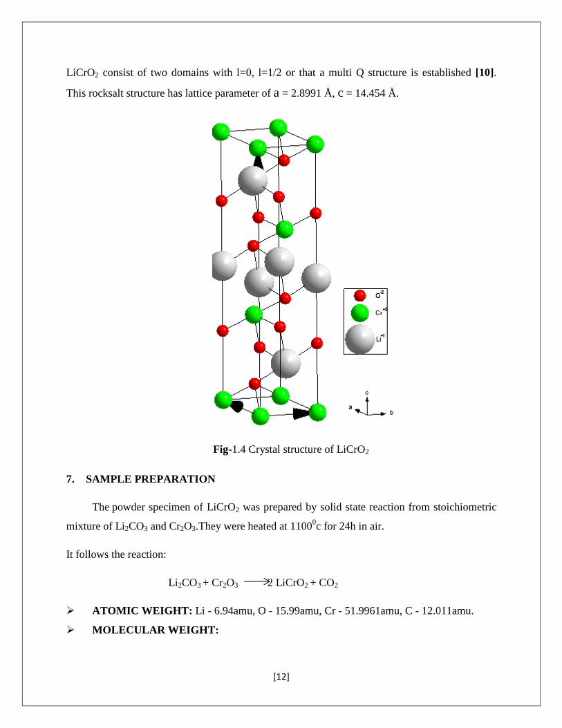
LiCrO2 consist of two domains with l=0, l=1/2 or that a multi Q structure is established [10].

This rocksalt structure has lattice parameter of a = 2.8991 Å, c = 14.454 Å.

7. SAMPLE PREPARATION

The powder specimen of LiCrO2 was prepared by solid state reaction from stoichiometric

mixture of Li2CO3 and Cr2O3.They were heated at 11000c for 24h in air.

It follows the reaction:

Li2CO3 + Cr2O3 2 LiCrO2 + CO2

ATOMIC WEIGHT: Li - 6.94amu, O - 15.99amu, Cr - 51.9961amu, C - 12.011amu.

MOLECULAR WEIGHT:

Fig-1.4 Crystal structure of LiCrO2

[13]

LiCrO2 = 6.94 + 51.9961 + 2 × (15.999) = 90.9341g

Li2CO3 = 2× (6.94) +12.011+3 × (15.999) = 73.888g

½ Li2CO3 = 36.9444g

Cr2O3 = 2 × 51.9961 + 3 × 15.999 = 151.9892g

½ Cr2O3 = 75.9946g

For 2g of LiCrO2, required Li2CO3 is = (36.944/90.9341) × 2 = 0.81254469 g

For 2g of LiCrO2, required Cr2O3 is = (75.9946/90.9341) ×2 = 1.671421g

7.1. SYNTHESIS OF LiCr0.95 Fe0.05 O2:

2g of LiCr0.95Fe0.05O2 prepared by solid state reaction method with 0.81829g of Li2CO3, 1.5844g

of Cr2O3 and 0.08761g of Fe2O3.

Followed by the equation-

0.5Li2CO3 + 0.475Cr2O3 + 0.025Fe2O3 LiCr0.95Fe0.05O2 + 0.5CO2

Molecular weight of Fe2O3 = 2 × 55.845 + 3 × 15.999

= 111.69 + 47.997 = 159.687g

Molecular weight of LiCr0.95Fe0.05O2 = 6.94 + (0.95) × 51.9961 + (0.05) × 55.845 + 2 × 15.999

= 91.12645g

7.2. SYNTHESIS OF LiCr0.98Fe0.02O2:

2g of LiCr0.98Fe0.02O2 prepared by solid state reaction method with 0.405928 g of

Li2CO3,1.6366075g of Cr2O3,0.017548g of Fe2O3.

Followed by the equation-

0.5Li2CO3 + 0.49Cr2O3 + 0.015Fe2O3 LiCr0.98Fe0.02O2 + 0.5CO2

Molecular weight of LiCr0.98Fe0.02O2 = 6.94 + (0.98) ×51.9961+ (0.02) × 55.845 + 2 × 15.999

=91.011078g

[14]

Li2CO3

(0.810g )

Cr2O3

(1.584g)

1.584g

Fe2O3

(0.084g)

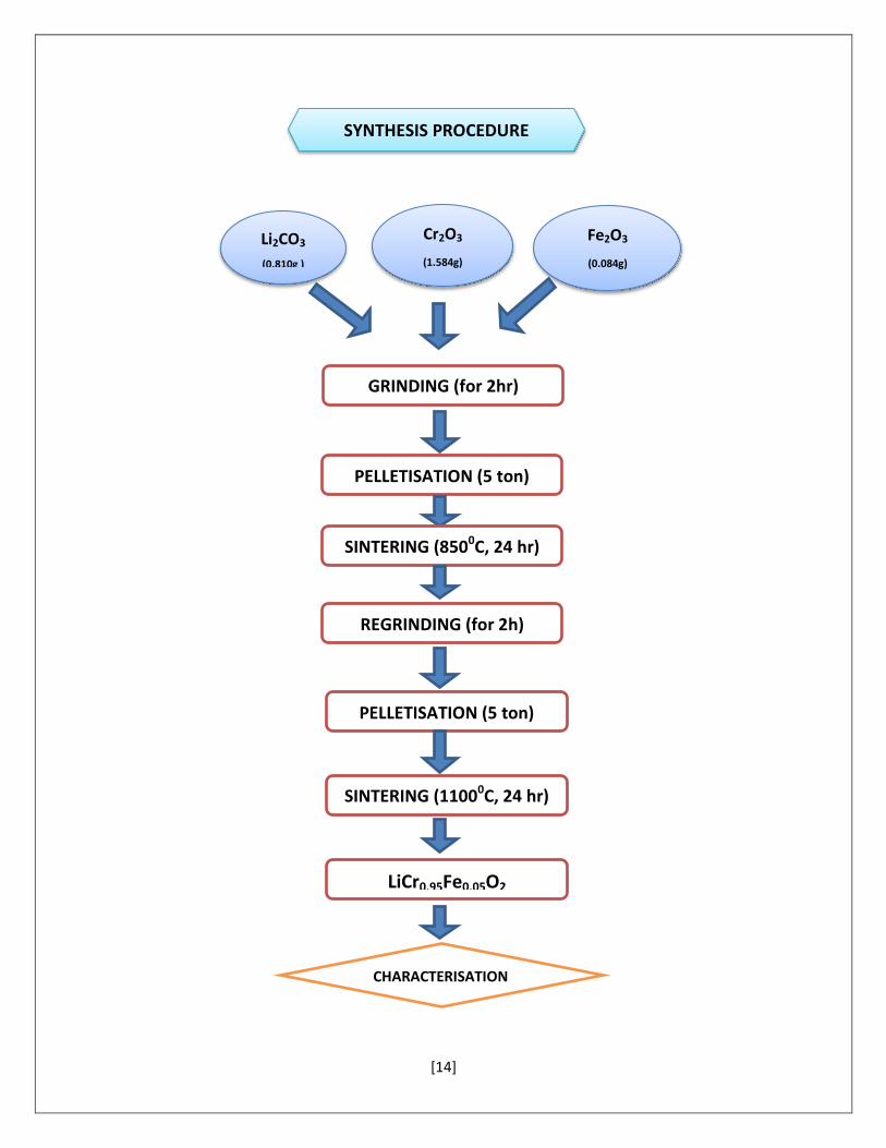
SYNTHESIS PROCEDURE

PELLETISATION (5 ton)

pressure)

SINTERING (8500C, 24 hr)

REGRINDING (for 2h)

PELLETISATION (5 ton)

PELLETISATION (5 ton pressure)

LiCr0.95Fe0.05O2

SINTERING (11000C, 24 hr)

CHARACTERISATION

N

GRINDING (for 2hr)

BREAKING OF PELLETS

BREAKING OF

PELLETS

[15]

Similarly, LiCr0.98Fe0.02O2 was also prepared following the above procedure.

PRESSING

At first all the sample are grounded in a mortar pestle for 2h in order to maintain uniform size,

then pellets were made by using 10mm diameter of stainless steel die set. We use hydrolic

pressed to apply pressure to the powder sample that is of 5 tons. As a result we get a pallets of

thickness 1mm.

SINTERING

The pellets were sintered at 850 0C for 2 hours. The ramping rate for cooling and heating was

kept at 5 ˚C/min. Then after first sintering the pellets were broken, again ground for half an hour

and again pellets were made. Then it was kept in furnace for second sintering at 1100˚C for 24

hours keeping heating rate the same.

8. CHARACTERISATION TECHNIQUES

8.1 X-ray Diffraction

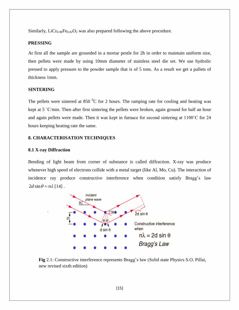
Bending of light beam from corner of substance is called diffraction. X-ray was produce

whenever high speed of electrons collide with a metal target (like Al, Mo, Cu). The interaction of

incidence ray produce constructive interference when condition satisfy Bragg’s law

nd sin2 [14] .

.

Fig 2.1: Constructive interference represents Bragg’s law (Solid state Physics S.O. Pillai,

new revised sixth edition)

)

[16]

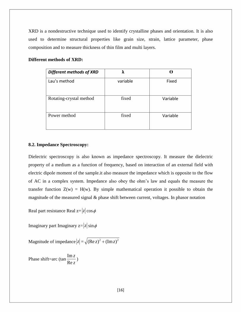
XRD is a nondestructive technique used to identify crystalline phases and orientation. It is also

used to determine structural properties like grain size, strain, lattice parameter, phase

composition and to measure thickness of thin film and multi layers.

Different methods of XRD:

Different methods of XRD λ Ө

Lau’s method variable

Fixed

Rotating-crystal method

fixed Variable

Power method

fixed Variable

8.2. Impedance Spectroscopy:

Dielectric spectroscopy is also known as impedance spectroscopy. It measure the dielectric

property of a medium as a function of frequency, based on interaction of an external field with

electric dipole moment of the sample.it also measure the impedance which is opposite to the flow

of AC in a complex system. Impedance also obey the ohm’s law and equals the measure the

transfer function Z(w) = H(w). By simple mathematical operation it possible to obtain the

magnitude of the measured signal & phase shift between current, voltages. In phasor notation

Real part resistance Real z= z cos

Imaginary part Imaginary z= z sin

Magnitude of impedance z =22 )(Im)(Re zz

Phase shift=arc (tanz

z

Re

Im)

[17]

The nature of dielectric material is that dielectric constant decreases with increases in frequency,

and constant at higher frequency. The decrease in frequency is due to polarization .This

polarization are of three types: 1) Electronic polarization

2) Ionic polarization

3) Dipolar polarization

Variation of polarization can be explained in the basis of relaxation times of above various

polarization process. The relaxation time minimum for electronic polarization but maximum for

dipolar polarization .

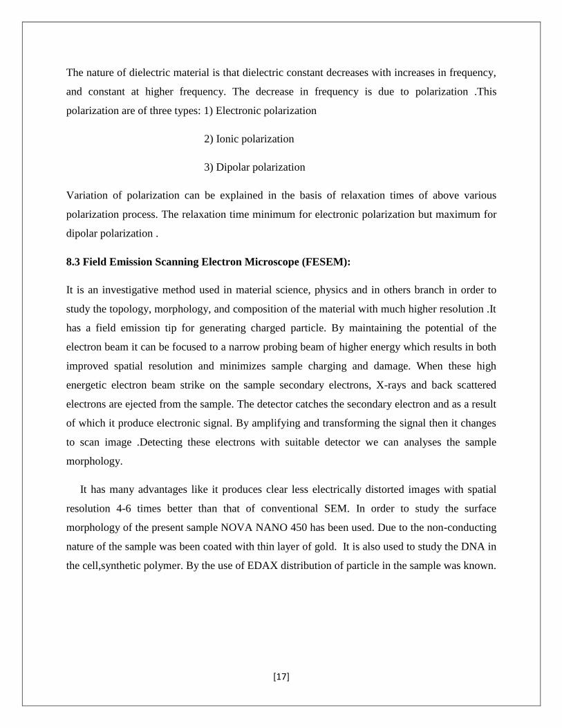
8.3 Field Emission Scanning Electron Microscope (FESEM):

It is an investigative method used in material science, physics and in others branch in order to

study the topology, morphology, and composition of the material with much higher resolution .It

has a field emission tip for generating charged particle. By maintaining the potential of the

electron beam it can be focused to a narrow probing beam of higher energy which results in both

improved spatial resolution and minimizes sample charging and damage. When these high

energetic electron beam strike on the sample secondary electrons, X-rays and back scattered

electrons are ejected from the sample. The detector catches the secondary electron and as a result

of which it produce electronic signal. By amplifying and transforming the signal then it changes

to scan image .Detecting these electrons with suitable detector we can analyses the sample

morphology.

It has many advantages like it produces clear less electrically distorted images with spatial

resolution 4-6 times better than that of conventional SEM. In order to study the surface

morphology of the present sample NOVA NANO 450 has been used. Due to the non-conducting

nature of the sample was been coated with thin layer of gold. It is also used to study the DNA in

the cell,synthetic polymer. By the use of EDAX distribution of particle in the sample was known.

[18]

Fig2.2: Schematic diagram of FESEM (www.intechopen.com)

8.4 UV-Vis Spectroscopy:

It generally refers to absorption, reflection spectroscopy in UV-visible spiral region. The

absorption or reflection in visible range directly effects the color of the chemicals involved. In

the region of electromagnetic spectrum molecules undergoes electronic transition .This technique

is while absorbance transition is from the ground state to the excited state. Most of the molecule

transition from the to *, it is the best method for determination of impurities in organic

molecules. The additional peaks can be observed due to impurities in the standard raw material.

We are calculating the band gap by using Tauc equation, which is given as:

)()( /1

g

n EhAh

Where n = 1/2 for direct band gap, n = 2 for indirect band gap.

[19]

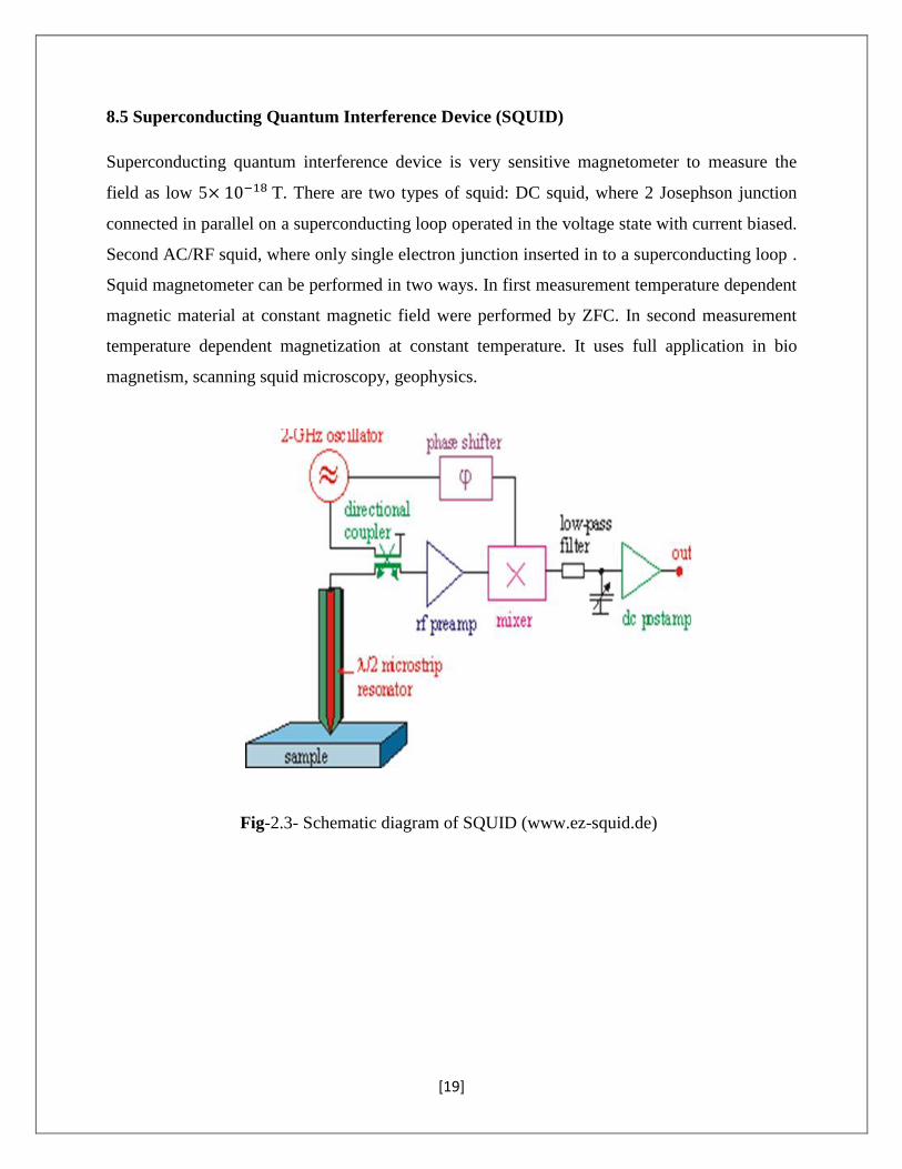
8.5 Superconducting Quantum Interference Device (SQUID)

Superconducting quantum interference device is very sensitive magnetometer to measure the

field as low 5 T. There are two types of squid: DC squid, where 2 Josephson junction

connected in parallel on a superconducting loop operated in the voltage state with current biased.

Second AC/RF squid, where only single electron junction inserted in to a superconducting loop .

Squid magnetometer can be performed in two ways. In first measurement temperature dependent

magnetic material at constant magnetic field were performed by ZFC. In second measurement

temperature dependent magnetization at constant temperature. It uses full application in bio

magnetism, scanning squid microscopy, geophysics.

Fig-2.3- Schematic diagram of SQUID (www.ez-squid.de)

[20]

9. RESULTS AND DISCUSSION

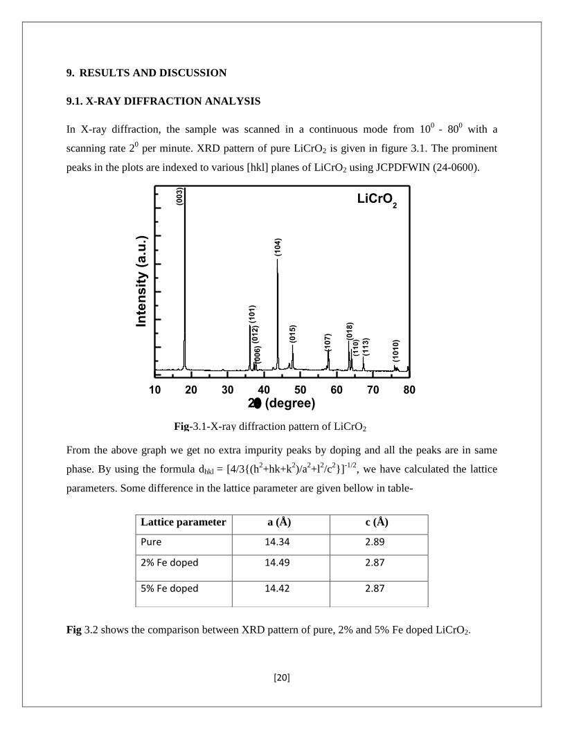
9.1. X-RAY DIFFRACTION ANALYSIS

In X-ray diffraction, the sample was scanned in a continuous mode from 100

- 800 with a

scanning rate 20 per minute. XRD pattern of pure LiCrO2 is given in figure 3.1. The prominent

peaks in the plots are indexed to various [hkl] planes of LiCrO2 using JCPDFWIN (24-0600).

From the above graph we get no extra impurity peaks by doping and all the peaks are in same

phase. By using the formula dhkl = [4/3{(h2+hk+k

2)/a

2+l

2/c

2}]

-1/2, we have calculated the lattice

parameters. Some difference in the lattice parameter are given bellow in table-

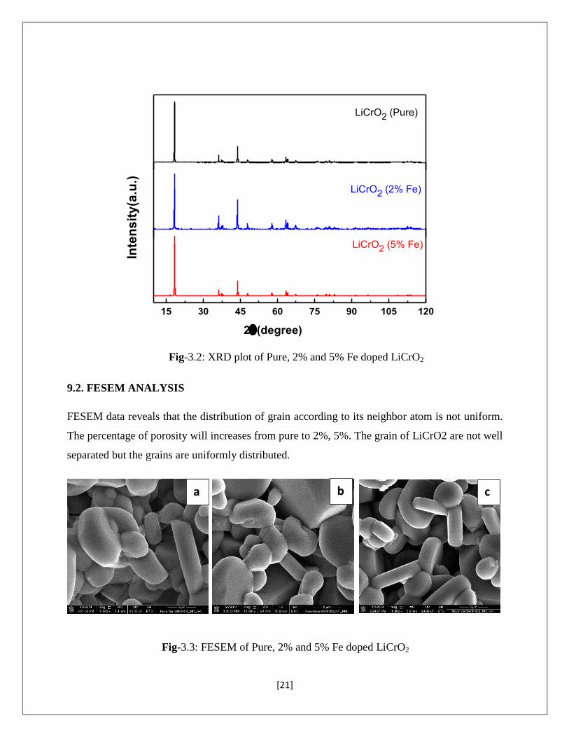
Fig 3.2 shows the comparison between XRD pattern of pure, 2% and 5% Fe doped LiCrO2.

Lattice parameter a (Å) c (Å)

Pure 14.34 2.89

2% Fe doped 14.49 2.87

5% Fe doped 14.42 2.87

Fig-3.1-X-ray diffraction pattern of LiCrO2

10 20 30 40 50 60 70 80

(113)

(11

0)

(1010)(0

18)

(107)

(015)

(006)

(012)

(104)

(101)

(003)

Inte

nsit

y (

a.u

.)

2 (degree)

LiCrO2

[21]

9.2. FESEM ANALYSIS

FESEM data reveals that the distribution of grain according to its neighbor atom is not uniform.

The percentage of porosity will increases from pure to 2%, 5%. The grain of LiCrO2 are not well

separated but the grains are uniformly distributed.

Pure LiCrO2

Fig-3.2: XRD plot of Pure, 2% and 5% Fe doped LiCrO2

15 30 45 60 75 90 105 120

LiCrO2 (Pure)

Inte

ns

ity

(a.u

.)

2(degree)

LiCrO2 (2% Fe)

LiCrO2 (5% Fe)

a b c

Fig-3.3: FESEM of Pure, 2% and 5% Fe doped LiCrO2

[22]

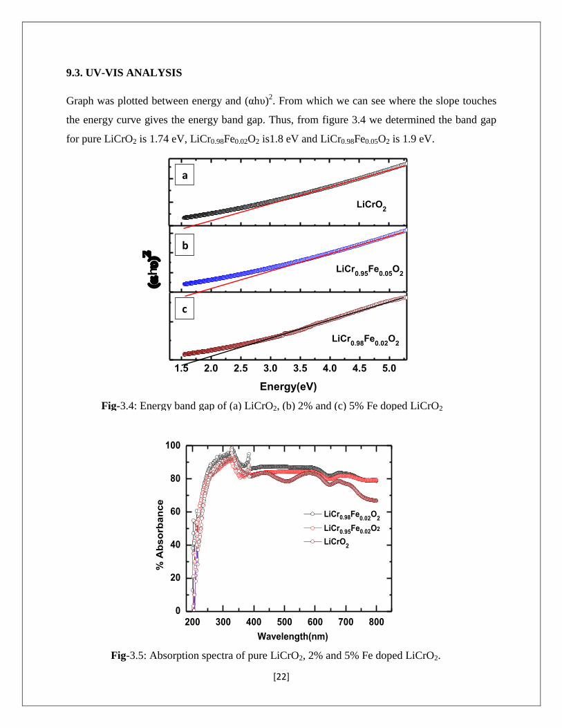
9.3. UV-VIS ANALYSIS

Graph was plotted between energy and (αhυ)2. From which we can see where the slope touches

the energy curve gives the energy band gap. Thus, from figure 3.4 we determined the band gap

for pure LiCrO2 is 1.74 eV, LiCr0.98Fe0.02O2 is1.8 eV and LiCr0.98Fe0.05O2 is 1.9 eV.

200 300 400 500 600 700 8000

20

40

60

80

100

% A

bso

rban

ce

Wavelength(nm)

LiCr0.98Fe0.02

O2

LiCr0.95Fe0.02O2

LiCrO2

Fig-3.4: Energy band gap of (a) LiCrO2, (b) 2% and (c) 5% Fe doped LiCrO2

Fig-3.5: Absorption spectra of pure LiCrO2, 2% and 5% Fe doped LiCrO2.

1.5 2.0 2.5 3.0 3.5 4.0 4.5 5.0

LiCr0.95

Fe0.05

O2

Energy(eV)

h

LiCr0.98

Fe0.02

O2

LiCrO2

a

b

c

[23]

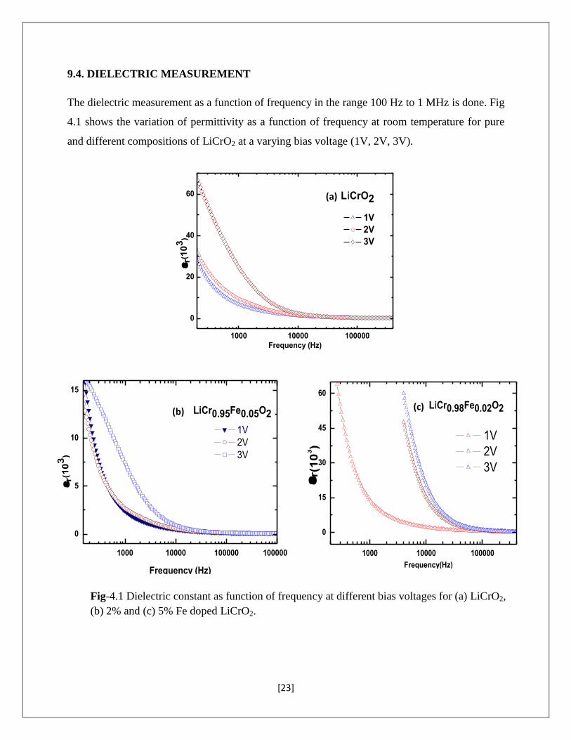
9.4. DIELECTRIC MEASUREMENT

The dielectric measurement as a function of frequency in the range 100 Hz to 1 MHz is done. Fig

4.1 shows the variation of permittivity as a function of frequency at room temperature for pure

and different compositions of LiCrO2 at a varying bias voltage (1V, 2V, 3V).

1000 10000 100000

0

20

40

60

r(

10

3)

Frequency (Hz)

1V

2V

3V

LiCrO2

Fig-4.1 Dielectric constant as function of frequency at different bias voltages for (a) LiCrO2,

(b) 2% and (c) 5% Fe doped LiCrO2.

1000 10000 100000

0

15

30

45

60

r(

10

3)

Frequency(Hz)

LiCr0.98Fe0.02O2

1V

2V

3V

1000 10000 100000 1000000

0

5

10

15

LiCr0.95Fe0.05O2

1V

2V

3V

r(

103

)

Frequency (Hz)

(a)

(b) (c)

[24]

100 1000 10000 100000

0

100

200

300

400

LiCrO2

LiCr0.98

Fe0.02

O2

LiCr0.95

Fe0.05

O2

r(

103)

Frequency(Hz)

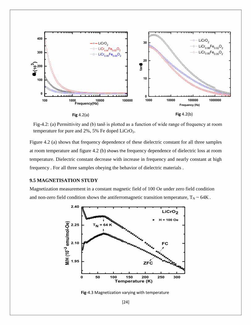
Figure 4.2 (a) shows that frequency dependence of these dielectric constant for all three samples

at room temperature and figure 4.2 (b) shows the frequency dependence of dielectric loss at room

temperature. Dielectric constant decrease with increase in frequency and nearly constant at high

frequency . For all three samples obeying the behavior of dielectric materials .

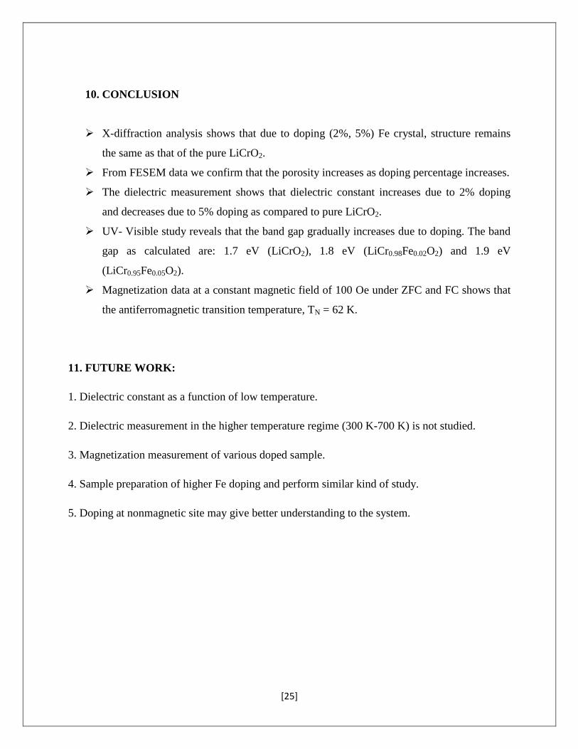
9.5 MAGNETISATION STUDY

Magnetization measurement in a constant magnetic field of 100 Oe under zero field condition

and non-zero field condition shows the antiferromagnetic transition temperature, TN ~ 64K .

0 50 100 150 200 250 300

1.95

2.10

2.25

2.40

M/H

(10

-3 e

mu

/mo

l-O

e)

Temperature (K)

H = 100 Oe

LiCrO2

FC

ZFC

TN = 64 K

1000 10000 100000 10000000

10

20

30

tan

Frequency (Hz)

LiCrO2

LiCr0.98

Fe0.02

O2

LiCr0.95Fe0.05

O2

Fig 4.2(a) Fig 4.2(b)

Fig-4.3 Magnetization varying with temperature

Fig-4.2: (a) Permittivity and (b) tanδ is plotted as a function of wide range of frequency at room

temperature for pure and 2%, 5% Fe doped LiCrO2.

[25]

10. CONCLUSION

X-diffraction analysis shows that due to doping (2%, 5%) Fe crystal, structure remains

the same as that of the pure LiCrO2.

From FESEM data we confirm that the porosity increases as doping percentage increases.

The dielectric measurement shows that dielectric constant increases due to 2% doping

and decreases due to 5% doping as compared to pure LiCrO2.

UV- Visible study reveals that the band gap gradually increases due to doping. The band

gap as calculated are: 1.7 eV (LiCrO2), 1.8 eV (LiCr0.98Fe0.02O2) and 1.9 eV

(LiCr0.95Fe0.05O2).

Magnetization data at a constant magnetic field of 100 Oe under ZFC and FC shows that

the antiferromagnetic transition temperature, TN = 62 K.

11. FUTURE WORK:

1. Dielectric constant as a function of low temperature.

2. Dielectric measurement in the higher temperature regime (300 K-700 K) is not studied.

3. Magnetization measurement of various doped sample.

4. Sample preparation of higher Fe doping and perform similar kind of study.

5. Doping at nonmagnetic site may give better understanding to the system.

[26]

11. REFERENCE

1) Introduction to Solid State Physics, Charles Kittel, Wiley Student’s 7th Edition and solid

state physics V. K. Babbar, R.K. Puri.

2) D. I. Khomskii, Bull. Am. Phys. Soc. C 21.002 (2001).

3) Classifying multiferroics: Mechanisms and effects, D. Khomskii, Phys. 77, 50937 (2009).

4) M. Fiebig, J. Phys. D Appl. Phys. 38, R123 73, 235113(2006)

5) Special issue, J. Phys. Condens. Matter 20, 434201 (2008).

6) R. Ramesh and N. A Spaldin, Nature Mater. 6, 21 (2007);

7) J. Zhai et al., Appl. Phys. Lett. 88, 062510 (2006).

8) G. X. Feng, L. F. Li, J. Y. Liu, N. Liu, H. Li, X. Q. Yang, X. J. Huang, L. Q. Chen, K. W.

Nam and W.S. Yoon J.Mater.chem,19, 2993 (2009).

9) S. Seki, Y.Onose and Y.Tokura Cond-mat. Str-el arXiv:0801.3151V(2008)

10) H. Kadowaki et al., J. Phys.: Condens. Matter 7, 6869 (1995)

11) Fig-2.1-constuctive interference represent BRAGG’S LAW (Introduction to Solid State

Physics, Charles Kittel, Wiley Student’s 7th Edition)

12) Fig2.2-Schematic diagram of FESEM (www.intechopen.com)

13) Fig-2.3- Schematic diagram of SQUID (www.ez-squid.de)

14) Element of x-ray diffraction by B.D.CULLITY