Syntax - Data Analysis and Statistical Software | Stata€¦ · · 2014-12-10power twoproportions — Power analysis for a two-sample proportions test ... Syntax Compute sample

Title stata.com

power twoproportions — Power analysis for a two-sample proportions test

Syntax Menu Description OptionsRemarks and examples Stored results Methods and formulas ReferencesAlso see

Syntax

Compute sample size

power twoproportions p1 p2[, power(numlist) options

]

Compute power

power twoproportions p1 p2 , n(numlist)[

options]

Compute effect size and experimental-group proportion

power twoproportions p1 , n(numlist) power(numlist)[

options]

where p1 is the proportion in the control (reference) group, and p2 is the proportion in the experimental(comparison) group. p1 and p2 may each be specified either as one number or as a list of valuesin parentheses (see [U] 11.1.8 numlist).

1

http://stata.com

http://www.stata.com/manuals13/u11.pdf#u11.1.8numlist





2 power twoproportions — Power analysis for a two-sample proportions test

options Description

test(test) specify the type of test; default is test(chi2)

Main∗alpha(numlist) significance level; default is alpha(0.05)∗power(numlist) power; default is power(0.8)∗beta(numlist) probability of type II error; default is beta(0.2)∗n(numlist) total sample size; required to compute power or effect size∗n1(numlist) sample size of the control group∗n2(numlist) sample size of the experimental group∗nratio(numlist) ratio of sample sizes, N2/N1; default is nratio(1), meaning

equal group sizescompute(n1 | n2) solve for N1 given N2 or for N2 given N1

nfractional allow fractional sample sizes∗diff(numlist) difference between the experimental-group and

control-group proportions, p2 − p1; specify instead of theexperimental-group proportion p2

∗ratio(numlist) ratio of the experimental-group proportion to thecontrol-group proportion, p2/p1; specify instead of theexperimental-group proportion p2

∗rdiff(numlist) risk difference, p2 − p1; synonym for diff()∗rrisk(numlist) relative risk, p2/p1; synonym for ratio()∗oratio(numlist) odds ratio, {p2(1− p1)}/{p1(1− p2)}effect(effect) specify the type of effect to display; default is

effect(diff)

continuity apply continuity correction to the normal approximationof the discrete distribution

direction(upper|lower) direction of the effect for effect-size determination; default isdirection(upper), which means that the postulated valueof the parameter is larger than the hypothesized value

onesided one-sided test; default is two sidedparallel treat number lists in starred options as parallel when

multiple values per option are specified (do notenumerate all possible combinations of values)

Table[no]table

[(tablespec)

]suppress table or display results as a table;

see [PSS] power, tablesaving(filename

[, replace

]) save the table data to filename; use replace to overwrite

existing filename

Graph

graph[(graphopts)

]graph results; see [PSS] power, graph













http://www.stata.com/manuals13/psspower.pdf#psspowertwoproportionsSyntaxtablespec

http://www.stata.com/manuals13/psspowertable.pdf#psspower,table

http://www.stata.com/manuals13/u11.pdf#u11.6Filenamingconventions

http://www.stata.com/manuals13/psspowergraph.pdf#psspower,graphSyntaxgraphopts

http://www.stata.com/manuals13/psspowergraph.pdf#psspower,graph

power twoproportions — Power analysis for a two-sample proportions test 3

Iteration

init(#) initial value for sample sizes or experimental-group proportioniterate(#) maximum number of iterations; default is iterate(500)

tolerance(#) parameter tolerance; default is tolerance(1e-12)

ftolerance(#) function tolerance; default is ftolerance(1e-12)[no]log suppress or display iteration log[

no]dots suppress or display iterations as dots

notitle suppress the title

∗Starred options may be specified either as one number or as a list of values; see [U] 11.1.8 numlist.notitle does not appear in the dialog box.

test Description

chi2 Pearson’s chi-squared test; the defaultlrchi2 likelihood-ratio testfisher Fisher–Irwin’s exact conditional test

test() does not appear in the dialog box. The dialog box selected is determined by the test() specification.

effect Description

diff difference between proportions, p2 − p1; the defaultratio ratio of proportions, p2/p1rdiff risk difference, p2 − p1rrisk relative risk, p2/p1oratio odds ratio, {p2(1− p1)}/{p1(1− p2)}

where tablespec is

column[:label

] [column

[:label

] [. . .] ] [

, tableopts]

column is one of the columns defined below, and label is a column label (may contain quotes andcompound quotes).


http://www.stata.com/manuals13/psspower.pdf#psspowertwoproportionsSyntaxcolumn

http://www.stata.com/manuals13/psspowertable.pdf#psspower,tableSyntaxtableopts



column Description Symbol

alpha significance level αalpha a observed significance level αapower power 1− βbeta type II error probability βN total number of subjects NN1 number of subjects in the control group N1

N2 number of subjects in the experimental group N2

nratio ratio of sample sizes, experimental to control N2/N1

delta effect size δp1 control-group proportion p1p2 experimental-group proportion p2diff difference between the experimental-group proportion p2 − p1

and the control-group proportionratio ratio of the experimental-group proportion to p2/p1

the control-group proportionrdiff risk difference p2 − p1rrisk relative risk p2/p1oratio odds ratio θtarget target parameter; synonym for p2all display all supported columns

Column beta is shown in the default table in place of column power if specified.Column alpha a is available when the test(fisher) option is specified.Columns nratio, diff, ratio, rdiff, rrisk, and oratio are shown in the default table if specified.

MenuStatistics > Power and sample size

Description

power twoproportions computes sample size, power, or the experimental-group proportionfor a two-sample proportions test. By default, it computes sample size for given power and thevalues of the control-group and experimental-group proportions. Alternatively, it can compute powerfor given sample size and values of the control-group and experimental-group proportions or theexperimental-group proportion for given sample size, power, and the control-group proportion. Alsosee [PSS] power for a general introduction to the power command using hypothesis tests.

Optionstest(test) specifies the type of the test for power and sample-size computations. test is one of chi2,

lrchi2, or fisher.

chi2 requests computations for the Pearson’s χ2 test. This is the default test.

lrchi2 requests computations for the likelihood-ratio test.

fisher requests computations for Fisher–Irwin’s exact conditional test. Iteration options are notallowed with this test.

http://www.stata.com/manuals13/psspower.pdf#psspower


� � �Main �

alpha(), power(), beta(), n(), n1(), n2(), nratio(), compute(), nfractional; see[PSS] power.

diff(numlist) specifies the difference between the experimental-group proportion and the control-group proportion, p2 − p1. You can specify either the experimental-group proportion p2 as acommand argument or the difference between the two proportions in diff(). If you specifydiff(#), the experimental-group proportion is computed as p2 = p1 + #. This option is notallowed with the effect-size determination and may not be combined with ratio(), rdiff(),rrisk(), or oratio().

ratio(numlist) specifies the ratio of the experimental-group proportion to the control-group proportion,p2/p1. You can specify either the experimental-group proportion p2 as a command argument orthe ratio of the two proportions in ratio(). If you specify ratio(#), the experimental-groupproportion is computed as p2 = p1×#. This option is not allowed with the effect-size determinationand may not be combined with diff(), rdiff(), rrisk(), or oratio().

rdiff(numlist) specifies the risk difference p2 − p1. This is a synonym for the diff() option,except the results are labeled as risk differences. This option is not allowed with the effect-sizedetermination and may not be combined with diff(), ratio(), rrisk(), or oratio().

rrisk(numlist) specifies the relative risk or risk ratio p2 − p1. This is a synonym for the ratio()option, except the results are labeled as relative risks. This option is not allowed with the effect-sizedetermination and may not be combined with diff(), ratio(), rdiff(), or oratio().

oratio(numlist) specifies the odds ratio {p2(1 − p1)}/{p1(1 − p2)}. You can specify ei-ther the experimental-group proportion p2 as a command argument or the odds ratio inoratio(). If you specify oratio(#), the experimental-group proportion is computed asp2 = 1/{1 + (1− p1)/(p1 × #)}. This option is not allowed with the effect-size determinationand may not be combined with diff(), ratio(), rdiff(), or rrisk().

effect(effect) specifies the type of the effect size to be reported in the output as delta. effect isone of diff, ratio, rdiff, rrisk, or oratio. By default, the effect size delta is the differencebetween proportions. If diff(), ratio(), rdiff(), rrisk(), or oratio() is specified, theeffect size delta will contain the effect corresponding to the specified option. For example, iforatio() is specified, delta will contain the odds ratio.

continuity requests that continuity correction be applied to the normal approximation of the discretedistribution. continuity cannot be specified with test(fisher) or test(lrchi2).

direction(), onesided, parallel; see [PSS] power.

� � �Table �

table, table(tablespec), notable; see [PSS] power, table.

saving(); see [PSS] power.

� � �Graph �

graph, graph(); see [PSS] power, graph. Also see the column table for a list of symbols used bythe graphs.

� � �Iteration �

init(#) specifies the initial value for the estimated parameter. For sample-size determination, theestimated parameter is either the control-group size N1 or, if compute(n2) is specified, theexperimental-group size N2. For the effect-size determination, the estimated parameter is the













experimental-group proportion p2. The default initial values for sample sizes for a two-sided testare based on the corresponding one-sided large-sample z test with the significance level α/2. Thedefault initial value for the experimental-group proportion is computed using the bisection method.

iterate(), tolerance(), ftolerance(), log, nolog, dots, nodots; see [PSS] power.

The following option is available with power twoproportions but is not shown in the dialog box:

notitle; see [PSS] power.

Remarks and examples stata.com

Remarks are presented under the following headings:

IntroductionUsing power twoproportionsComputing sample sizeComputing powerComputing effect size and experimental-group proportionTesting a hypothesis about two independent proportions

This entry describes the power twoproportions command and the methodology for power andsample-size analysis for a two-sample proportions test. See [PSS] intro for a general introduction topower and sample-size analysis and [PSS] power for a general introduction to the power commandusing hypothesis tests.

IntroductionThe comparison of two independent proportions arises in studies involving two independent

binomial populations. There are many examples of studies where a researcher would like to comparetwo independent proportions. A pediatrician might be interested in the relationship between lowbirthweight and the mothers’ use of a particular drug during pregnancy. He or she would like totest the null hypothesis that there is no difference in the proportion of low-birthweight babies formothers who took the drug and mothers who did not. A drug manufacturer may want to test thedeveloped new topical treatment for a foot fungus by testing the null hypothesis that the proportionof successfully treated patients is the same in the treatment and placebo groups.

Hypothesis testing of binomial outcomes relies on a set of assumptions: 1) a Bernoulli outcomeis observed a fixed number of times; 2) the probability p of observing an event of interest in onetrial is fixed across all trials; and 3) individual trials are independent. Each of the two populationsmust conform to the assumptions of a binomial distribution.

This entry describes power and sample-size analysis for the inference about two populationproportions performed using hypothesis testing. Specifically, we consider the null hypothesis H0 :p2 = p1 versus the two-sided alternative hypothesis Ha: p2 6= p1, the upper one-sided alternativeHa: p2 > p1, or the lower one-sided alternative Ha: p2 < p1.

The large-sample Pearson’s χ2 and likelihood-ratio tests are commonly used to test hypothesesabout two independent proportions. The test of Fisher (1935) and Irwin (1935) is commonly used tocompare the two proportions in small samples.

The power twoproportions command provides power and sample-size analysis for these threetests. For Fisher’s exact test, the direct computation is available only for the power of the test.Estimates of the sample size and effect size for Fisher’s exact test are difficult to compute directlybecause of the discrete nature of the sampling distribution of the test statistic. They can, however, beobtained indirectly on the basis of the power computation; see example 8 for details.



http://stata.com

http://www.stata.com/manuals13/pssintro.pdf#pssintro



Using power twoproportions

power twoproportions computes sample size, power, or experimental-group proportion for atwo-sample proportions test. All computations are performed for a two-sided hypothesis test where,by default, the significance level is set to 0.05. You may change the significance level by specifyingthe alpha() option. You can specify the onesided option to request a one-sided test. By default,all computations assume a balanced or equal-allocation design; see [PSS] unbalanced designs for adescription of how to specify an unbalanced design.

power twoproportions performs power analysis for three different tests, which can be specifiedwithin the test() option. The default is Pearson’s χ2 test (test(chi2)), which approximatesthe sampling distribution of the test statistic by the standard normal distribution. You may insteadrequest computations based on the likelihood-ratio test by specifying the test(lrchi2) option.To request Fisher’s exact conditional test based on the hypergeometric distribution, you can specifytest(fisher). The fisher method is not available for computing sample size or effect size; seeexample 8 for details.

To compute the total sample size, you must specify the control-group proportion p1, the experimental-group proportion p2, and, optionally, the power of the test in the power() option. The default poweris set to 0.8.

Instead of the total sample size, you can compute one of the group sizes given the other one. Tocompute the control-group sample size, you must specify the compute(n1) option and the samplesize of the experimental group in the n2() option. Likewise, to compute the experimental-groupsample size, you must specify the compute(n2) option and the sample size of the control group inthe n1() option.

To compute power, you must specify the total sample size in the n() option, the control-groupproportion p1, and the experimental-group proportion p2.

Instead of the experimental-group proportion p2, you can specify other alternative measures ofeffect when computing sample size or power; see Alternative ways of specifying effect below.

To compute effect size and the experimental-group proportion, you must specify the total samplesize in the n() option, the power in the power() option, the control-group proportion p1, andoptionally, the direction of the effect. The direction is upper by default, direction(upper), whichmeans that the experimental-group proportion is assumed to be larger than the specified control-groupvalue. You can change the direction to be lower, which means that the experimental-group proportionis assumed to be smaller than the specified control-group value, by specifying the direction(lower)option.

There are multiple definitions of the effect size for a two-sample proportions test. The effect()option specifies what definition power twoproportions should use when reporting the effect size,which is labeled as delta in the output of the power command. The available definitions are thedifference between the experimental-group proportion and the control-group proportion (diff), the ratioof the experimental-group proportion to the control-group proportion (ratio), the risk difference p2−p1(rdiff), the relative risk p2/p1 (rrisk), and the odds ratio {p2(1− p1)}/{p1(1− p2)} (oratio).When effect() is specified, the effect size delta contains the estimate of the corresponding effectand is labeled accordingly. By default, delta corresponds to the difference between proportions. Ifany of the options diff(), ratio(), rdiff(), rrisk(), or oratio() are specified and effect()is not specified, delta will contain the effect size corresponding to the specified option.

Instead of the total sample size n(), you can specify individual group sizes in n1() and n2(), orspecify one of the group sizes and nratio() when computing power or effect size. Also see Twosamples in [PSS] unbalanced designs for more details.

http://www.stata.com/manuals13/pssunbalanceddesigns.pdf#pssunbalanceddesigns

http://www.stata.com/manuals13/pssunbalanceddesigns.pdf#pssunbalanceddesignsRemarksandexamplesTwosamples




Alternative ways of specifying effect

As we mentioned above, power twoproportions provides a number of ways to specify thedisparity between the control-group and experimental-group proportions for sample-size and powerdeterminations.

You can specify the control-group proportion p1 and the experimental-group proportion p2 directly,after the command name:

power twoproportions p1 p2 , . . .

For this specification, the default effect size delta displayed by the power command is thedifference p2 − p1 between the proportions. You can use the effect() option to request anothertype of effect. For example, if you specify effect(oratio),

power twoproportions p1 p2 , effect(oratio) . . .

the effect size delta will correspond to the odds ratio.

Alternatively, you can specify the control-group proportion p1 and one of the options diff(),ratio(), rdiff(), rrisk(), or oratio(). For these specifications, the effect size delta willcontain the effect corresponding to the option. If desired, you can change this by specifying theeffect() option.

Specify difference p2 − p1 between the two proportions:

power twoproportions p1 , diff(numlist) . . .

Specify risk difference p2 − p1:

power twoproportions p1 , rdiff(numlist) . . .

Specify ratio p2/p1 of the two proportions:

power twoproportions p1 , ratio(numlist) . . .

Specify relative risk or risk ratio p2/p1:

power twoproportions p1 , rrisk(numlist) . . .

Specify odds ratio {p2(1− p1)}/{p1(1− p2)}:

power twoproportions p1 , oratio(numlist) . . .

In the following sections, we describe the use of power twoproportions accompanied byexamples for computing sample size, power, and experimental-group proportions.

Computing sample size

To compute sample size, you must specify the control-group proportion p1, the experimental-groupproportion p2, and, optionally, the power of the test in the power() option. A default power of 0.8is assumed if power() is not specified.

Example 1: Sample size for a two-sample proportions test

Consider a study investigating the effectiveness of aspirin in reducing the mortality rate due tomyocardial infarction (heart attacks). Let pA denote the proportion of deaths for aspirin users in thepopulation and pN denote the corresponding proportion for nonusers. We are interested in testing thenull hypothesis H0: pA − pN = 0 against the two-sided alternative hypothesis Ha: pA − pN 6= 0.







Previous studies indicate that the proportion of deaths due to heart attacks is 0.015 for nonusersand 0.001 for users. Investigators wish to determine the minimum sample size required to detect anabsolute difference of |0.001− 0.015| = 0.014 with 80% power using a two-sided 5%-level test.

To compute the required sample size, we specify the values 0.015 and 0.001 as the control-and experimental-group proportions after the command name. We omit options alpha(0.05) andpower(0.8) because the specified values are their respective defaults.

. power twoproportions 0.015 0.001

Performing iteration ...

Estimated sample sizes for a two-sample proportions testPearson’s chi-squared testHo: p2 = p1 versus Ha: p2 != p1

Study parameters:

alpha = 0.0500power = 0.8000delta = -0.0140 (difference)

p1 = 0.0150p2 = 0.0010

Estimated sample sizes:

N = 1270N per group = 635

A total sample of 1,270 individuals, 635 individuals per group, must be obtained to detect an absolutedifference of 0.014 between proportions of aspirin users and nonusers with 80% power using atwo-sided 5%-level Pearson’s χ2 test.

Example 2: Alternative ways of specifying effect

The displayed effect size delta in example 1 is the difference between the experimental-groupproportion and the control-group proportion. We can redefine the effect size to be, for example, theodds ratio by specifying the effect() option.

. power twoproportions 0.015 0.001, effect(oratio)



Study parameters:

alpha = 0.0500power = 0.8000delta = 0.0657 (odds ratio)

p1 = 0.0150p2 = 0.0010



The effect size delta now contains the estimated odds ratio and is labeled correspondingly.

Instead of the estimate of the proportion in the experimental group, we may have an estimateof the odds ratio {p2(1 − p1)}/{p1(1 − p2)}. For example, the estimate of the odds ratio in thisexample is 0.0657. We can specify the value of the odds ratio in the oratio() option instead ofspecifying the experimental-group proportion 0.001:


. power twoproportions 0.015, oratio(0.0657)



Study parameters:

alpha = 0.0500power = 0.8000delta = 0.0657 (odds ratio)

p1 = 0.0150p2 = 0.0010

odds ratio = 0.0657



The results are identical to the prior results. The estimate of the odds ratio is now displayed in theoutput, and the effect size delta now corresponds to the odds ratio.

We can also specify the following measures as input parameters: difference between proportionsin the diff() option, risk difference in the rdiff() option, ratio of the proportions in the ratio()option, or relative risk in the rrisk() option.

Example 3: Likelihood-ratio test

Instead of the Pearson’s χ2 test as in example 1, we can compute sample size for the likelihood-ratiotest by specifying the test(lrchi2) option.

. power twoproportions 0.015 0.001, test(lrchi2)


Estimated sample sizes for a two-sample proportions testLikelihood-ratio testHo: p2 = p1 versus Ha: p2 != p1

Study parameters:


p1 = 0.0150p2 = 0.0010



The required total sample size of 1,062 is smaller than that for the Pearson’s χ2 test.

Example 4: Computing one of the group sizes

Suppose we anticipate a sample of 600 aspirin users and wish to compute the required numberof nonusers given the study parameters from example 1. We specify the number of aspirin users inn2(), and we also include compute(n1):


. power twoproportions 0.015 0.001, n2(600) compute(n1)



Study parameters:


p1 = 0.0150p2 = 0.0010N2 = 600


N = 1317N1 = 717

We require a sample of 717 nonusers given 600 aspirin users for a total of 1,317 subjects. The totalnumber of subjects is larger for this unbalanced design compared with the corresponding balanceddesign in example 1.

Example 5: Unbalanced design

By default, power twoproportions computes sample size for a balanced or equal-allocationdesign. If we know the allocation ratio of subjects between the groups, we can compute the requiredsample size for an unbalanced design by specifying the nratio() option.

Continuing with example 1, we will suppose that we anticipate to recruit twice as many aspirinusers as nonusers; that is, n2/n1 = 2. We specify the nratio(2) option to compute the requiredsample size for the specified unbalanced design.

. power twoproportions 0.015 0.001, nratio(2)



Study parameters:


p1 = 0.0150p2 = 0.0010

N2/N1 = 2.0000


N = 1236N1 = 412N2 = 824

We need a total sample size of 1,236 subjects.

Also see Two samples in [PSS] unbalanced designs for more examples of unbalanced designs fortwo-sample tests.




Computing power

To compute power, you must specify the total sample size in the n() option, the control-groupproportion p1, and the experimental-group proportion p2.

Example 6: Power of a two-sample proportions test

Continuing with example 1, we will suppose that we anticipate a sample of only 1,100 subjects.To compute the power corresponding to this sample size given the study parameters from example1, we specify the sample size in n():

. power twoproportions 0.015 0.001, n(1100)

Estimated power for a two-sample proportions testPearson’s chi-squared testHo: p2 = p1 versus Ha: p2 != p1

Study parameters:

alpha = 0.0500N = 1100

N per group = 550delta = -0.0140 (difference)

p1 = 0.0150p2 = 0.0010

Estimated power:

power = 0.7416

With a smaller sample of 1,100 subjects, we obtain a lower power of 74% compared with example 1.

Example 7: Multiple values of study parameters

In this example, we would like to assess the effect of varying the proportion of aspirin users on thepower of our study. Suppose that the total sample size is 1,100 with equal allocation between groups,and the value of the proportion in the nonusing group is 0.015. We specify a range of proportionsfor aspirin users from 0.001 to 0.009 with a step size of 0.001 as a numlist in parentheses as thesecond argument of the command:

. power twoproportions 0.015 (0.001(0.001)0.009), n(1100)

Estimated power for a two-sample proportions testPearson’s chi-squared testHo: p2 = p1 versus Ha: p2 != p1

alpha power N N1 N2 delta p1 p2

.05 .7416 1100 550 550 -.014 .015 .001

.05 .6515 1100 550 550 -.013 .015 .002

.05 .5586 1100 550 550 -.012 .015 .003

.05 .4683 1100 550 550 -.011 .015 .004

.05 .3846 1100 550 550 -.01 .015 .005

.05 .3102 1100 550 550 -.009 .015 .006

.05 .2462 1100 550 550 -.008 .015 .007

.05 .1928 1100 550 550 -.007 .015 .008

.05 .1497 1100 550 550 -.006 .015 .009



From the table, the power decreases from 74% to 15% as the proportion of deaths for aspirin usersincreases from 0.001 to 0.009 or the absolute value of the effect size (measured as the differencebetween the proportion of deaths for aspirin users and that for nonusers) decreases from 0.014 to0.006.

For multiple values of parameters, the results are automatically displayed in a table, as we seeabove. For more examples of tables, see [PSS] power, table. If you wish to produce a power plot,see [PSS] power, graph.

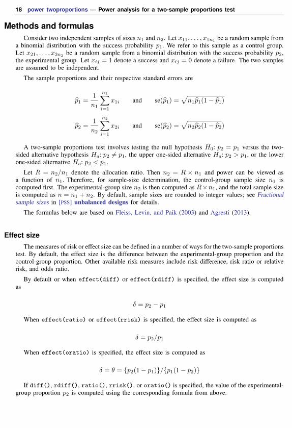
Example 8: Saw-toothed power function

We can also compute power for the small-sample Fisher’s exact conditional test. The samplingdistribution of the test statistic for this test is discrete. As such, Fisher’s exact test shares the sameissues arising with power and sample-size analysis as described in detail for the binomial one-sampleproportion test in example 7 of [PSS] power oneproportion. In particular, the power function ofFisher’s exact test has a saw-toothed shape as a function of the sample size. Here, we demonstrate thesaw-toothed shape of the power function and refer you to example 7 of [PSS] power oneproportionfor details.

Let’s plot powers of the Fisher’s exact test for a range of experimental-group sizes between 50and 65 given the control-group proportion of 0.6, the experimental-group proportion of 0.25, andthe control-group size of 25. We specify the graph() option to produce a graph and the table()option to produce a table; see [PSS] power, graph and [PSS] power, table for more details about thegraphical and tabular outputs from power. Within graph(), we specify options to request that thereference line be plotted on the y axis at a power of 0.8 and that the data points be labeled withthe corresponding sample sizes. Within table(), we specify the formats() option to display onlythree digits after the decimal point for the power and alpha a columns.

. power twoproportions 0.6 0.25, test(fisher) n1(25) n2(50(1)65)> graph(yline(0.8) plotopts(mlabel(N)))> table(, formats(alpha_a "%7.3f" power "%7.3f"))

Estimated power for a two-sample proportions testFisher’s exact testHo: p2 = p1 versus Ha: p2 != p1

alpha alpha_a power N N1 N2 delta p1 p2

.05 0.026 0.771 75 25 50 -.35 .6 .25

.05 0.025 0.793 76 25 51 -.35 .6 .25

.05 0.026 0.786 77 25 52 -.35 .6 .25

.05 0.026 0.782 78 25 53 -.35 .6 .25

.05 0.025 0.804 79 25 54 -.35 .6 .25

.05 0.026 0.793 80 25 55 -.35 .6 .25

.05 0.028 0.786 81 25 56 -.35 .6 .25

.05 0.025 0.814 82 25 57 -.35 .6 .25

.05 0.025 0.802 83 25 58 -.35 .6 .25

.05 0.025 0.797 84 25 59 -.35 .6 .25

.05 0.028 0.823 85 25 60 -.35 .6 .25

.05 0.026 0.813 86 25 61 -.35 .6 .25

.05 0.026 0.807 87 25 62 -.35 .6 .25

.05 0.025 0.819 88 25 63 -.35 .6 .25

.05 0.028 0.821 89 25 64 -.35 .6 .25

.05 0.027 0.816 90 25 65 -.35 .6 .25



http://www.stata.com/manuals13/psspoweroneproportion.pdf#psspoweroneproportionRemarksandexamplesex7

http://www.stata.com/manuals13/psspoweroneproportion.pdf#psspoweroneproportion

http://www.stata.com/manuals13/psspoweroneproportion.pdf#psspoweroneproportionRemarksandexamplesex7

http://www.stata.com/manuals13/psspoweroneproportion.pdf#psspoweroneproportion




50

51

52

53

54

55

56

57

58

59

60

61

62

6364

65

.77

.78

.79

.8

.81

.82

Pow

er (

1−β)

50 55 60 65Experimental−group sample size (N2)

Parameters: α = .05, N1 = 25, δ = −.35, p1 = .6, p2 = .25

Fisher’s exact testH0: p2 = p1 versus Ha: p2 ≠ p1

Estimated power for a two−sample proportions test

Figure 1. Saw-toothed power function

The power is not a monotonic function of the sample size. Also from the table, we see that all theobserved significance levels are smaller than the specified level of 0.05.

Because of the saw-toothed nature of the power curve, obtaining an optimal sample size becomestricky. For example, if we wish to have power of 80%, then from the above table and graph, we seethat potential experimental-group sample sizes are 54, 57, 58, 60, and so on. One may be temptedto choose the smallest sample size for which the power is at least 80%. This, however, would notguarantee that the power is at least 80% for any larger sample size. Instead, Chernick and Liu (2002)suggest selecting the smallest sample size after which the troughs of the power curve do not go belowthe desired power. Following this recommendation in our example, we would pick a sample size of60, which corresponds to the observed significance level of 0.028 and power of 0.823.

Computing effect size and experimental-group proportion

There are multiple definitions of the effect size for a two-sample proportions test. By default, effectsize δ is defined as the difference between the experimental-group proportion and the control-groupproportion, δ = p2 − p1, also known as a risk difference. Other available measures of the effect sizeare the ratio of the experimental-group proportion to the control-group proportion δ = p2/p1, alsoknown as a relative risk or risk ratio, and the odds ratio δ = {p2(1− p1)}/{p1(1− p2)}.

Sometimes, we may be interested in determining the smallest effect and the correspondingexperimental-group proportion that yield a statistically significant result for prespecified sample sizeand power. In this case, power, sample size, and control-group proportion must be specified. Inaddition, you must also decide on the direction of the effect: upper, meaning p2 > p1, or lower,meaning p2 < p1. The direction may be specified in the direction() option; direction(upper)is the default.

The underlying computations solve the corresponding power equation for the value of theexperimental-group proportion given power, sample size, and other study parameters. The effectsize is then computed from the specified control-group proportion and the computed experimental-group proportion using the corresponding functional relationship. The difference between proportionsis reported by default, but you can request other measures by specifying the effect() option.


Example 9: Minimum detectable change in the experimental-group proportion

Continuing with example 6, we will compute the smallest change in the proportion of deaths foraspirin users less than that for nonusers that can be detected given a total sample of 1,100 individualsand 80% power. To solve for the proportion of aspirin users in the experimental group, after thecommand name, we specify the control group (nonaspirin users), proportion of 0.015, total samplesize n(1100), and power power(0.8):

. power twoproportions 0.015, n(1100) power(0.8) direction(lower)


Estimated experimental-group proportion for a two-sample proportions testPearson’s chi-squared testHo: p2 = p1 versus Ha: p2 != p1; p2 < p1

Study parameters:

alpha = 0.0500power = 0.8000


p1 = 0.0150

Estimated effect size and experimental-group proportion:

delta = -0.0147 (difference)p2 = 0.0003

We find that given the proportion of nonusers of 0.015, the smallest (in absolute value) differencebetween proportions that can be detected in this study is −0.0147, which corresponds to the proportionof aspirin users of 0.0003.

Although the difference between proportions is reported by default, we can request that anotherrisk measure be reported by specifying the effect() option. For example, we can request that theodds ratio be reported instead:

. power twoproportions 0.015, n(1100) power(0.8) direction(lower) effect(oratio)


Estimated experimental-group proportion for a two-sample proportions testPearson’s chi-squared testHo: p2 = p1 versus Ha: p2 != p1; p2 < p1

Study parameters:

alpha = 0.0500power = 0.8000


p1 = 0.0150

Estimated effect size and experimental-group proportion:

delta = 0.0195 (odds ratio)p2 = 0.0003

The corresponding value of the odds ratio in this example is 0.0195.

In these examples, we computed the experimental-group proportion assuming a lower direction,p2 < p1, which required you to specify the direction(lower) option. By default, experimental-group proportion is computed for an upper direction, meaning that the proportion is greater than thespecified value of the control-group proportion.


Testing a hypothesis about two independent proportions

After the initial planning, we collect data and wish to test the hypothesis that the proportionsfrom two independent populations are the same. We can use the prtest command to perform suchhypothesis tests; see [R] prtest for details.

Example 10: Two-sample proportions test

Consider a 2 × 3 contingency table provided in table 2.1 of Agresti (2013, 38). The table isobtained from a report by the Physicians’ Health Study Research Group at Harvard Medical Schoolthat investigated the relationship between aspirin use and heart attacks.

The report presents summary data on fatal and nonfatal heart attacks. In the current example, wecombine these two groups into a single group representing the total cases with heart attacks for aspirinusers and nonusers. The estimated proportion of heart attacks in the control group, nonaspirin users,is 189/11034 = 0.0171 and in the experimental group, aspirin users, is 104/11037 = 0.0094.

. prtesti 11034 0.0171 11037 0.0094

Two-sample test of proportions x: Number of obs = 11034y: Number of obs = 11037

Variable Mean Std. Err. z P>|z| [95% Conf. Interval]

x .0171 .0012342 .014681 .019519y .0094 .0009185 .0075997 .0112003

diff .0077 .0015385 .0046846 .0107154under Ho: .0015393 5.00 0.000

diff = prop(x) - prop(y) z = 5.0023Ho: diff = 0

Ha: diff < 0 Ha: diff != 0 Ha: diff > 0Pr(Z < z) = 1.0000 Pr(|Z| < |z|) = 0.0000 Pr(Z > z) = 0.0000

Let pA and pN denote the proportions of heart attacks in the population for aspirin users andnonusers, respectively. From the above results, we find a statistically significant evidence to reject thenull hypothesis H0: pA = pN versus a two-sided alternative Ha: pA 6= pN at the 5% significancelevel; the p-value is very small.

We use the parameters of this study to perform a sample-size analysis we would have conductedbefore the study.

. power twoproportions 0.0171 0.0094



Study parameters:


p1 = 0.0171p2 = 0.0094


N = 6922N per group = 3461

http://www.stata.com/manuals13/rprtest.pdf#rprtest


We find that for Pearson’s χ2 test, a total sample size of 6,922, assuming a balanced design, is requiredto detect the difference between the control-group proportion of 0.0171 and the experimental-groupproportion of 0.0094 with 80% power using a 5%-level two-sided test.

Stored resultspower twoproportions stores the following in r():

Scalarsr(alpha) significance levelr(alpha a) actual significance level of the Fisher’s exact testr(power) powerr(beta) probability of a type II errorr(delta) effect sizer(N) total sample sizer(N a) actual sample sizer(N1) sample size of the control groupr(N2) sample size of the experimental groupr(nratio) ratio of sample sizes, N2/N1

r(nratio a) actual ratio of sample sizesr(nfractional) 1 if nfractional is specified; 0 otherwiser(onesided) 1 for a one-sided test; 0 otherwiser(p1) control-group proportionr(p2) experimental-group proportionr(diff) difference between the experimental- and control-group proportionsr(ratio) ratio of the experimental-group proportion to the control-group proportionr(rdiff) risk differencer(rrisk) relative riskr(oratio) odds ratior(separator) number of lines between separator lines in the tabler(divider) 1 if divider is requested in the table; 0 otherwiser(init) initial value for sample sizes or experimental-group proportionr(continuity) 1 if continuity correction is used; 0 otherwiser(maxiter) maximum number of iterationsr(iter) number of iterations performedr(tolerance) requested parameter tolerancer(deltax) final parameter tolerance achievedr(ftolerance) requested distance of the objective function from zeror(function) final distance of the objective function from zeror(converged) 1 if iteration algorithm converged; 0 otherwise

Macrosr(type) testr(method) twoproportionsr(test) chi2, lrchi2, or fisherr(direction) upper or lowerr(columns) displayed table columnsr(labels) table column labelsr(widths) table column widthsr(formats) table column formats

Matrixr(pss table) table of results


Methods and formulasConsider two independent samples of sizes n1 and n2. Let x11, . . . , x1n1 be a random sample from

a binomial distribution with the success probability p1. We refer to this sample as a control group.Let x21, . . . , x2n2

be a random sample from a binomial distribution with the success probability p2,the experimental group. Let xij = 1 denote a success and xij = 0 denote a failure. The two samplesare assumed to be independent.

The sample proportions and their respective standard errors are

p1 =1

n1

n1∑i=1

x1i and se(p1) =√n1p1(1− p1)

p2 =1

n2

n2∑i=1

x2i and se(p2) =√n2p2(1− p2)

A two-sample proportions test involves testing the null hypothesis H0: p2 = p1 versus the two-sided alternative hypothesis Ha: p2 6= p1, the upper one-sided alternative Ha: p2 > p1, or the lowerone-sided alternative Ha: p2 < p1.

Let R = n2/n1 denote the allocation ratio. Then n2 = R × n1 and power can be viewed asa function of n1. Therefore, for sample-size determination, the control-group sample size n1 iscomputed first. The experimental-group size n2 is then computed as R×n1, and the total sample sizeis computed as n = n1 + n2. By default, sample sizes are rounded to integer values; see Fractionalsample sizes in [PSS] unbalanced designs for details.

The formulas below are based on Fleiss, Levin, and Paik (2003) and Agresti (2013).

Effect sizeThe measures of risk or effect size can be defined in a number of ways for the two-sample proportions

test. By default, the effect size is the difference between the experimental-group proportion and thecontrol-group proportion. Other available risk measures include risk difference, risk ratio or relativerisk, and odds ratio.

By default or when effect(diff) or effect(rdiff) is specified, the effect size is computedas

δ = p2 − p1

When effect(ratio) or effect(rrisk) is specified, the effect size is computed as

δ = p2/p1

When effect(oratio) is specified, the effect size is computed as

δ = θ = {p2(1− p1)}/{p1(1− p2)}

If diff(), rdiff(), ratio(), rrisk(), or oratio() is specified, the value of the experimental-group proportion p2 is computed using the corresponding formula from above.

http://www.stata.com/manuals13/pssunbalanceddesigns.pdf#pssunbalanceddesignsRemarksandexamplesFractionalsamplesizes

http://www.stata.com/manuals13/pssunbalanceddesigns.pdf#pssunbalanceddesignsRemarksandexamplesFractionalsamplesizes



Pearson’s chi-squared test

For a large sample size, a binomial process can be approximated by a normal distribution. Theasymptotic sampling distribution of the test statistic

z =(p2 − p1)− (p2 − p1)√p(1− p)

(1n1

+ 1n2

)is standard normal, where p = (n1p1 + n2p2)/(n1 + n2) is the pooled proportion and p is itsestimator. The square of this statistic, z2, has an approximate χ2 distribution with one degree offreedom, and the corresponding test is known as Pearson’s χ2 test.

Let α be the significance level, β be the probability of a type II error, and z1−α and zβ be the(1− α)th and the βth quantiles of the standard normal distribution.

Let σD =√p1(1− p1)/n1 + p2(1− p2)/n2 be the standard deviation of the difference between

proportions and σp =√p(1− p) (1/n1 + 1/n2) be the pooled standard deviation.

The power π = 1− β is computed using

π =

Φ{

(p2−p1)−c−z1−ασpσD

}for an upper one-sided test

Φ{

−(p2−p1)−c−z1−ασpσD

}for a lower one-sided test

Φ{

(p2−p1)−c−z1−α/2σpσD

}+ Φ

{−(p2−p1)−c−z1−α/2σp

σD

}for a two-sided test

(1)

where Φ(·) is the cdf of the standard normal distribution, and c is the normal-approximation continuitycorrection. For equal sample sizes, n1 = n2 = n/2, the continuity correction is expressed as c = 2/n(Levin and Chen 1999).

For a one-sided test, given the allocation ratio R = n2/n1, the total sample size n is computedby inverting the corresponding power equation in (1),

n =

{z1−α

√p(1− p)− zβ

√w2p1(1− p1) + w1p2(1− p2)

}2

w1w2 (p2 − p1)2 (2)

where w1 = 1/(1 +R) and w2 = R/(1 +R). Then n1 and n2 are computed as n1 = n/(1 +R)and n2 = R × n1, respectively. If the continuity option is specified, the sample size nc for aone-sided test is computed as

nc =n

4

(1 +

√1 +

2

nw1w2|p2 − p1|

)2

where n is the sample size computed without the correction. For unequal sample sizes, the continuitycorrection generalizes to c = 1/(2nw1w2) (Fleiss, Levin, and Paik 2003).

For a two-sided test, the sample size is computed by iteratively solving the two-sided powerequation in (1). The initial values for the two-sided computations are obtained from (2) with thesignificance level α/2.

If one of the group sizes is known, the other one is computed by iteratively solving the correspondingpower equation in (1). The initial values are obtained from (2) by assuming that R = 1.

The experimental-group proportion p2 is computed by iteratively solving the corresponding powerequations in (1). The default initial values are obtained by using a bisection method.


Likelihood-ratio testLet q1 = 1−p1, q2 = 1−p2, and q = 1−p = 1−(n1p1+n2p2)/(n1+n2). The likelihood-ratio

test statistic is given by

G =

√2n

{n1p1n

ln(p1p

)+n1q1n

ln(q1q

)+n2p2n

ln(p2p

)+n2q2n

ln(q2q

)}The power π = 1− β is computed using

π =

Φ (G− z1−α) for an upper one-sided testΦ (−G− z1−α) for a lower one-sided testΦ(G− z1−α/2

)+ Φ

(−G− z1−α/2

)for a two-sided test

(3)

For a one-sided test, given the allocation ratio R, the total sample size n is computed by invertingthe corresponding power equation in (3),

n =(z1−α − zβ)

2

2{w1p1 ln

(p1p

)+ w1q1 ln

(q1q

)+ w2p2 ln

(p2p

)+ w2q2 ln

(q2q

)} (4)

where w1 = 1/(1 +R) and w2 = R/(1 +R). Then n1 and n2 are computed as n1 = n/(1 +R)and n2 = R× n1, respectively.

For a two-sided test, the sample size is computed by iteratively solving the two-sided powerequation in (3). The initial values for the two-sided computations are obtained from equation (4) withthe significance level α/2.

If one of the group sizes is known, the other one is computed by iteratively solving the correspondingpower equation in (3). The initial values are obtained from (4) by assuming that R = 1.

The experimental-group proportion p2 is computed by iteratively solving the corresponding powerequations in (3). The default initial values are obtained by using a bisection method.

Fisher’s exact conditional testPower computation for Fisher’s exact test is based on Casagrande, Pike, and Smith (1978). We

present formulas from the original paper with a slight change in notation: we use p1 and p2 in placeof p1 and p2 and η in place of θ. The change in notation is to avoid confusion between our use ofgroup proportions p1 and p2 and their use in the paper—compared with our definitions, the roles ofp1 and p2 in the paper are reversed in the definitions of the hypotheses and other measures such asthe odds ratio. In our definitions, p1 = p2 is the proportion in the experimental group, p2 = p1 isthe proportion in the control group, and η = 1/θ. Also we denote n1 = n2 to be the sample size ofthe experimental group and n2 = n1 to be the sample size of the control group.

Let k be the number of successes in the experimental group, and let m be the total number ofsuccesses in both groups. The conditional distribution of k is given by

p(k|m, η) =

(n1

k

)(n2

m−k)ηk∑

i

(n1

i

)(n2

m−i)ηi

where η = {p1(1 − p2)}/{p2(1 − p1)}, and the range of i is given by L = max(0,m − n2) toU = min(n1,m).


Assume an upper one-sided test given by

H0: p1 = p2 versus Ha: p1 > p2 (5)

The hypothesis (5) in terms of η can be expressed as follows:

H0: η = 1 versus Ha: η > 1

Let ku be the critical value of k such that the following inequalities are satisfied:

U∑i=ku

p(i|m, η = 1) ≤ α andU∑

i=ku−1

p(i|m, η = 1) > α (6)

The conditional power is

β(η|m) =

U∑i=ku

p(i|m, η)

For a lower one-sided hypothesis Ha : p1 < p2, the corresponding hypothesis in terms of η isgiven by

H0: η = 1 versus Ha: η < 1

The conditional power in this case is

β(η|m) =

kl∑i=L

p(i|m, η)

where kl is the critical value of k such that the following inequalities are satisfied:

kl∑i=L

p(i|m, η = 1) ≤ α andkl+1∑i=L

p(i|m, η = 1) > α (7)

.

For a two-sided test, the critical values kl and ku are calculated using the inequalities (6) and (7)with α/2, respectively.

Finally, the unconditional power is calculated as

β(η) =∑j

β(η|j)P (j)

where j takes the value from 0 to n, and

P (j) =

U∑i=L

(n1i

)p1i(1− p1)n1−i

(n2j − i

)p2j−i(1− p2)n2−j+i

where L = max(0, j − n2) and U = min(n1, j).


ReferencesAgresti, A. 2013. Categorical Data Analysis. 3rd ed. Hoboken, NJ: Wiley.

Casagrande, J. T., M. C. Pike, and P. G. Smith. 1978. The power function of the “exact” test for comparing twobinomial distributions. Journal of the Royal Statistical Society, Series C 27: 176–180.

Chernick, M. R., and C. Y. Liu. 2002. The saw-toothed behavior of power versus sample size and software solutions:Single binomial proportion using exact methods. American Statistician 56: 149–155.

Fisher, R. A. 1935. The Design of Experiments. Edinburgh: Oliver & Boyd.

Fleiss, J. L., B. Levin, and M. C. Paik. 2003. Statistical Methods for Rates and Proportions. 3rd ed. New York:Wiley.

Irwin, J. O. 1935. Tests of significance for differences between percentages based on small numbers. Metron 12:83–94.

Levin, B., and X. Chen. 1999. Is the one-half continuity correction used once or twice to derive a well-knownapproximate sample size formula to compare two independent binomial distributions? American Statistician 53:62–66.

Also see[PSS] power — Power and sample-size analysis for hypothesis tests

[PSS] power, graph — Graph results from the power command

[PSS] power, table — Produce table of results from the power command

[PSS] Glossary[R] bitest — Binomial probability test

[R] prtest — Tests of proportions

http://www.stata.com/bookstore/smrp.html




http://www.stata.com/manuals13/pssglossary.pdf#pssGlossary

http://www.stata.com/manuals13/rbitest.pdf#rbitest

http://www.stata.com/manuals13/rprtest.pdf#rprtest

Documents

Syntax - Data Analysis and Statistical Software | Stata€¦ · · 2014-12-10power twoproportions — Power analysis for a two-sample proportions test ... Syntax Compute sample