<JClD-l960<?

SYNFUELS FROM FUSION -/USING THE TANDEM MIRROR REACTOR AND A THERMOCHEMICAL CVCLE TO PRODUCE HYDROGEN

-QSCLAMEn Edited by: Richard W. Werner

November 1 , 1982 O C I D - 1 S 6 0 9

DSS3 005216

A Collaborative Study by: Lawrence Livermore National Laboratory, P. 0. Box 808, Livermore, CA 94550:

Richard W. Werner (Principal Investigator) Edward N. C. Dalder David W, Dorn Robert G. Hickman Gary L. Johnson Oscar H. Krikorian R. Carroll Maninger

U. C. Davis, Department of Machanical Engineering, Davis, CA 95616: Myron A. Hoffman

University of Washington, Nuclear Engineering Department, Seattle, WA 98195: Fred L. Ribe (Principal Investigator) Gene L. Woodruff M. E. Abhold A. L. Babb Mike Lloid J. Oelund T. H. Zerguini

Rowe & Associates, 14400 Bellevue Redmond Rd. Suite 208, Bellevue, WA 98007: Don S. Rowe

General Atomic Co., P. 0. Box 81608, San Diego, CA 92138:

Lloyd C. Brown John H. Norman

NOTICE

PORTIONS OF THIS BEPORT ABE ULECIBlt i j work Performed for: fias been rcarori'ii-e-i frn" >"he bett available '/ Office of Fusion Energy copy to permit tfie broaden: -issitle ivtlfc U. S. Department of Energy •bility.

U. S. Department of Energy Contracts: W-7405-Eng-48 at the Lawrence Livermore National Laboratory; DE-AM0G-76RL 0222S and TA-DE AT06-76ET 52047 at the University of Washington.

i toBTMEUiiKi Of fha:.[_;. ';•:! ;s I I I M I T E D

PREFACE

Our study on synfuels is intended to focus primarily on the engineering aspects of coupling a tandem mirror fusion reactor (TMR) to a thermochemical cycle for the express purpose of producing hydrogen. The hydrogen is then to be used:

• As a portable fuel

• As a feedstock to synthesize other fuels such as gasoline or methanol

• To produce other useful hydrocarbons, NH 3, etc.

The detailed "how to" of hydrogen utilization is beyond the scope of this report. We have concentrated solely on the thermochemistry of the hydrogen production process, although a brief Section 12 discusses "Synfuels Beyond Hydrogen."

The physics data are supportive to the study and are based on the most recent plasma theory and experiment. The model used is that of the tandem mirror reactor and the physics parameters of MARS.

ii

TABLE OF CONTENTS

Title EXECUTIVE SUMMARY MOTIVATION FOR THE STUDY THE TANDEM MIRROR REACTOR AND ITS PHYSICS ENERGY BALANCE - THE TANDEM MIRROR REACTOR AS AN ENERGY SOURCE THE LITHIUM OXIDE CANISTER BLANKET SYSTEM HIGH-TEMPERATURE BLANKET ENERSY TRANSPORT SYSTEM - REACTOR TO PROCESS THERMOCHEMICAL HYDROGEN PROCESSES INTERFACING THE GA CYCLE MATCHING POWER AND TEMPERATURE DEMANDS - PERFORMANCE AND EFFICIENCY EVALUATIONS PRELIMINARY COST ESTIMATES SYNFUELS BEYOND HYDROGEN SIMULATION OF SECTION II OF GENERAL ATOMIC THERMOCHEMICAL CYCLE AND THE THERMODYNAMICS OF THE H„SO.-H,0 SYSTEM

iii

SECTION 1 EXECUTIVE SUMMARY

Contributor: R. W. Werner

TABLE OF CONTENTS ion Page

INTRODUCTION 1-1 HIGHLIGHTS 1-1 THE TANDEM MIRROR REACTOR DRIVER . . 1-4 THE THERMOCHEMICAL PLANT PROCESS 1-5 REACTOR BLANKET DESIGN, TKE CANISTER BLANKET WITH THE JOULE-BOOSTED DECOMPOSER - OUR OPTION 1 1-11 1.5.1 The Canister Structural Envelope: Data Summary

and Conclusions 1-17 1.5.2 The Canister Moderating Volume and Hot Shield 1-19 RECTOR BLANKET DESIGN, THE CANISTER/HIGH TEMPERATURE AXIALLY ZONED BLANKET WITH THE FLUIDIZED BED DECOMPOSER -OPTION 2 1-22 1.6.1 The Canister Structural Envelope: Data Summary

and Conclusions 1-24 1.6.2 The Canister High Temperature Region 1-24 1.6-3 General Conclusions 1-28 "IN SITU" TRITIUM CONTROL - PRODUCING A TRITIUM-FREE HYDROGEN PLANT 1-29

i

TABLE OF CONTENTS Section Page 1.8 PROGRESS IN NEUTRONICS 1-31 1.9 THE JOULE-BOOSTED DECOMPOSER . . . . . 1-32 1.10 THE FLUIDIZED BED DECOMPOSER 1-3Z 1.11 MATERIALS 1-36 1.12 A PLOT PLAN FOR THE HYDROGEN PLANT 1-38 1.13 PROGRESS IN MEETING THE HIGH TEMPERATURE REQUIREMENTS

OF THE PROCESS 1-38 1.14 MATCHING POWER AND TEMPERATURE OEMANDS - PERFORMANCE

AND EFFICIENCY EVALUATIONS FOR THE JOULE-BOOSTED DECOMPOSER 1-41 1.14.1 Option 1 1-41 1.14.2 Option 2 1-44

1.15 COST OF PRODUCING THE HYDROGEN 1-44 1.16 CHEMICAL PLANT OPERATIONAL DEPENDABILITY 1-46 1.17 PROBLEM AREAS 1-46 1.18 RECOMMENDATIONS FOR FUTURE STUDY 1-46

LIST OF TABLES Table Page 1.1 Design parameters for the Tandem Mirror Reactor as a

driver for the thermochemical plant 1-8 1.2 The Canister structural envelope and first wall data

summary 1-18 1.3 Summary of the Canister performance data 1-20 1.4 The high temperature Canister structural envelope and

first wall data summary 1-26 1.5 Summary of the high temperature Canister performance 1-27 1.6 Material candidates for handling process fluids

containing HI X and I2 1-37 1.7 Candidate materials of construction for sulfuric acid 1-39

LIST OF FIGURES Figure Page 1.1 The Tandem Mirror Reactor 1-6 1.2 Tandem Mirror Reactor (MARS) 1-7 1.3 Power balance of a Tandem Mirror Reactor used for

producing synfuels, Q = 25.D and M = 1.20 1-9 1.4 The General Atomic sulfur-iodine cycle 1-10 1.5 Cross section through the Canister blanket showing

its main features 1-12 1.6 Manifolding to ring headers is offset for assembly 1-14 1.7 Ring module assembly 1-15 1.8 The ring module installation is straightforward -

solenoids stay in place 1-16 1.9 Schematic of an axial-zoned TMR with low and high

temperature modules . . . . . 1-23

m

LIST OF FIGURES Figure f_a£e 1.10 Cross section illustration of the high temperature

blanket Canister 1-25 1.11 Isolation of the LigO from mainstream coolant provides

for "tritium-free" hydrogen product 1-30 1.12 Joule-Boosted decomposer 1-33 1.73 Equilibrium decomposition curves for SO3 1-34 1.14 Fluidized bed decomposer 1-35 1.15 Plot plan for the hydrogen plant „ 1-40 ^.>5 Pr&grevs iTi ttirerri-mj Vicmfcet Yempwature HTH! raiding

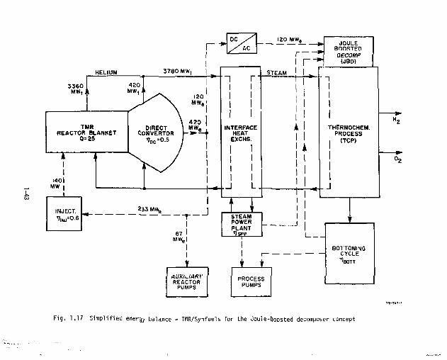
decomposer temperature 1-42 1.17 Simplified energy balance - TMR/Synfuels for the Joule-

Boosted decomposer concept 1-43 1.18 Power balance diagram for the Joule-Boosted decomposer

concept (with vapor recompression in Section III and some pressure staging in Section II) 1-S5

iv

1.0 EXECUTIVE SUMMARY

l.J INTRODUCTION

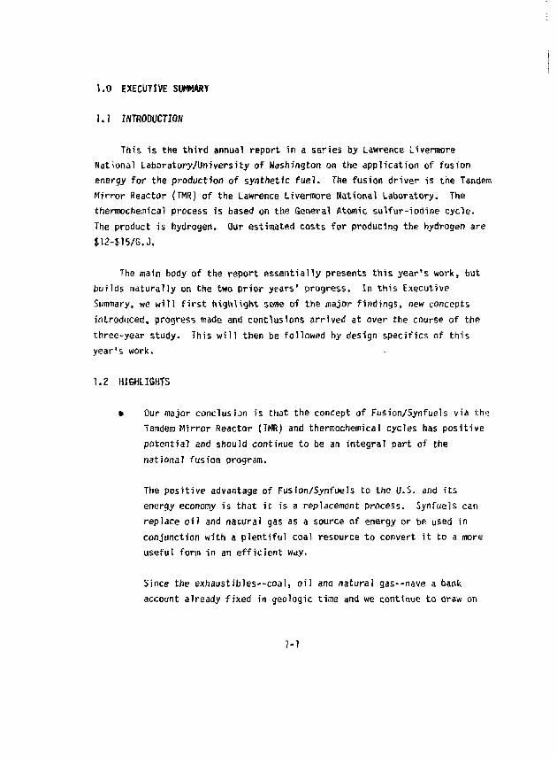
This is the third annual report in a series by Lawrence Livermore National Laboratory/University of Washington on the application of fusion energy for the production of synthetic fuel. The fusion driver is the Tandem Mirror Reactor (TMR) of the Lawrence Livermore National Laboratory. The thermoche.nical process is based on the General Atomic sulfur-iodine cycle. The product is hydrogen. Our estimated costs for producing the hydrogen are tl2-$15/G.J.

The main body of the report essentially presents this year's work, but builds naturally on the two prior years' progress. In this Executive Summary, we will first highlight sons of the major findings, new concepts introduced, progress made and conclusions arrived at over the course of the three-year study. This will then be followed by design specifics of this year's work.

1.2 HIGHLIGHTS

• Our major conclusion is that the concept of Fusion/Synfuels via the Tandem Mirror Reactor (TMR) and thermochemical cycles has positive potential and should continue to be an integral part of the national fusion program.

The positive advantage of Fusion/Synfuels to the U.S. and its energy economy is that it is a replacement process. Synfuels can replace oil and natural gas as a source of energy or be used in conjunction with a plentiful coal resource to convert it to a more useful form in an efficient way.

Since the exhaustibles--coal, oil and nature,] gas--have a bank account already fixed in geologic time and we continue to draw on

1-1

this bank account in ever increasing amount, it is important to begin to reverse this process. The reversal may be accomplished in two ways that are complementary:

Making use of Fusion/Electric, which reduces the demand on the exhaustibles

and Utilizing Fusion/Synfuels, which adds to the bank account.

t The production of hydrogen using thermochemical cycles continues to have a demonstrated experimental base at the laboratory level with positive progress. Production rates of 100 liters/hour have been achieved. Production rates of 10,000 liters/hour will occur in CY82 or by mid CY83 at Ispra, Italy, in the Christina project.

• A thermochemicaJ cycle for hydrogen production is a process in which water is used as the feedstock along with a non-fossil high temperature heat source to produce H 2 and Op as product gases. Three cycles of about 25 cycles proposed worldwide continue to dominate the production of W? from water. These cycles are:

1. The General Atomic Sulfure Iodine cycle (our design base)

2. The Westinghouse cycle

3. The Ispra cycle (our international collaboration backup).

• Potential drivers for these thermochemical cycles that can provide a viable energy source are limited. There are only three:

1. The fusion reactor

2. The HSTfi or VHTR

3. Solar.

1-2

• Of the three drivers, the '•usion reactor and the KGTR Continue to have an edge over solar concentrators due to the diurnal nature of solar and the need for thermochemical plants to be run on a continuous basis.

• Assuming that an economically competitive fusion reactor can be created, the reasons for using a fusion reactor in preference to the HGTR as an energy source for synfuol production wer e not addressed within the conte, of this study. Either could do the job. Both may be appropriate.

• The TMR has some advantage over the Tokamak for synfuels, due principally to its relatively sample central cell topology, when further progress is made in increaiing the Q of the TMRS it will have the additional advantage over both the Tokamak and the HGTR of directly supplying electricity for the bulk of the high temper­ature SO, decomposition process step rather than supplying high temperature via thermal energy. This will allow the reactor blanket to run substantially cooler.

• The design of a synfuel plant remains extremely complicated. It is large—like an oil refinery—and has many units to design, tn working on the des ign of the individual parts rather thgn the total complex we were justifiably encouragad, through our conceptual design results, to find that the components perceived to be the most dTv'ffcu ft—the SO? decomposer, tne ffgSff Goffer mot tt\e fusion reactor blanket--all had potentially good design solutions and also a credible materials base.

• The Fusion Reactor/Synfuel total plant complex is substantially more difficult to analyze than a Fusion Reac.jr/Electric;ai p.ant. In this area of anal :is we have done some significant work and made substantial contributions in developing standardized procedures for flow sheeting and for matching plant loaq lines and

1-3

temperatures to the energy source. The procedures will be useful for all combinations of energy sources and thermochemical plants.

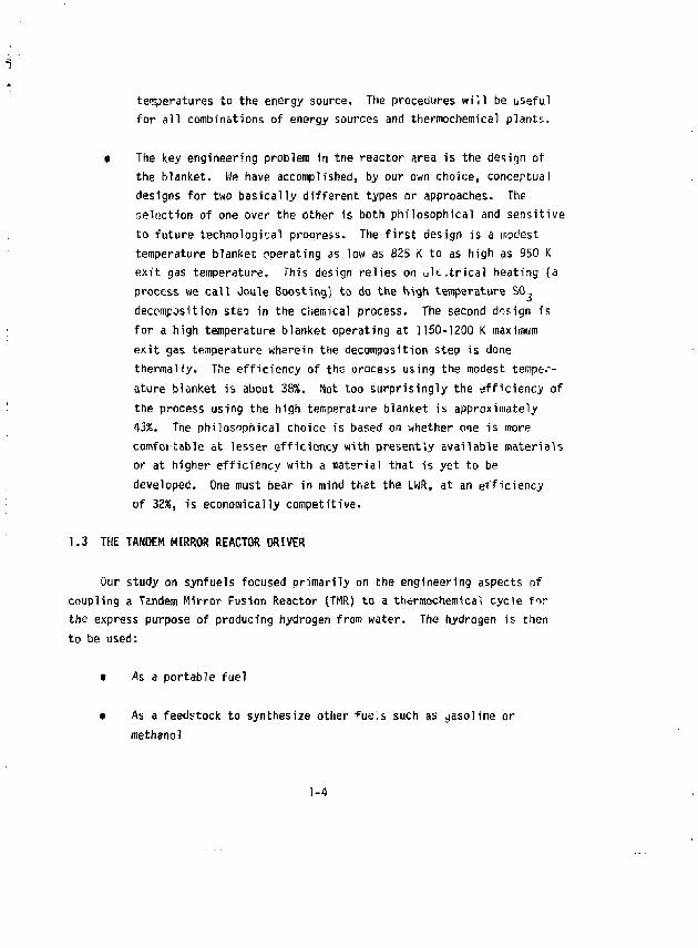
• The key engineering problem in tne reactor area is the design of the blanket. We have accomplished, by our own choice, conceptual designs for two basically different types or approaches. The selection of one over the other is both philosophical and sensitive to future technological proqress. The first design is a modest temperature blanket ^Derating as low as 825 K to as high as 950 K exit gas temperature. This design relies on ult.trical heating (a process we call Joule Boosting) to do the t\Sgh temperature SO, decomposition stes in the chemical process. The second design is for a high temperature blanket operating at 1150-1200 K maximum exit gas temperature wherein the decomposition step is done thermally. The efficiency of the process using the modest temper­ature blanket is about 38%. Not too surprisingly the efficiency of the process using the high temperature blanket is approximately 43%. The philosophical choice is based on whether one is more comfortable at lesser efficiency with presently available materials or at higher efficiency with a material that is yet to be developed. One must bear in mind that the LWR, at an efficiency of 32fc, is economically competitive.

1.3 THE TANOEM MIRROR REACTOR DRIVER

Our study on synfuels focused primarily on the engineering aspects of coupling a Tandem Mirror fusion Reactor (TMR) to a thcrmochemical cycle for the express purpose of producing hydrogen from water. The hydrogen is then to be used:

• As a portable fuel

• As a feedstock to synthesize other *ue,s such as gasoline or methanol

1-4

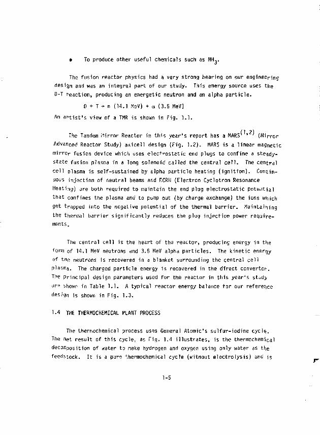
• To produce other useful chemicals such as NH

The fusion reactor physics had a very strong bearing on our engineering design and was an integral part of our study. This energy source uses the D-T reaction, producing an energetic neutron and an alpha particle.

D + T + n (14.1 MeV) + a (3.5 MeV) An artist's view of a TMR is shown in Fig. 1.1.

(1 2) The Tandem ilirror Reactor in this year's report has a MARS ' ' (Mirror Advanced Reactor Study) axicell design (Fig. 1.2). MARS is a linear magnetic mirror fusion device which uses electrostatic end plugs to confine a steady-state fusion plasma in a long solenoid called the central cell. The central cell plasma is self-sustained by alpha particle heating (ignition). Contin­uous injection of neutral beams ar.d ECRH (Electron Cyclotron Resonance Heating) are both required to maintain the end plug electrostatic potfe.itial that confines the plasma and to pump out (by charge exchange) the ions which get trapped into the negative potential of the thermal barrier. Maintaining the thermal barrier significantly reduces the plug injection power require­ments.

The central cell is the heart of the reactor, producing energy in the form of 14.1 MeV neutrons and 3.5 MeV alpha particles. The kinetic energy of the neutrons is recovered in a blanket surrounding the central cell plasma. The charged particle energy is recovered in the direct convertor-. The principal design parameters used for the reactor in this year's stud}/ arp shown in Table 1.1. A typical reactor energy balance for our reference design is shown in Fig. 1.3.

1.4 THE THERMOCHEMICAL PLANT PROCESS

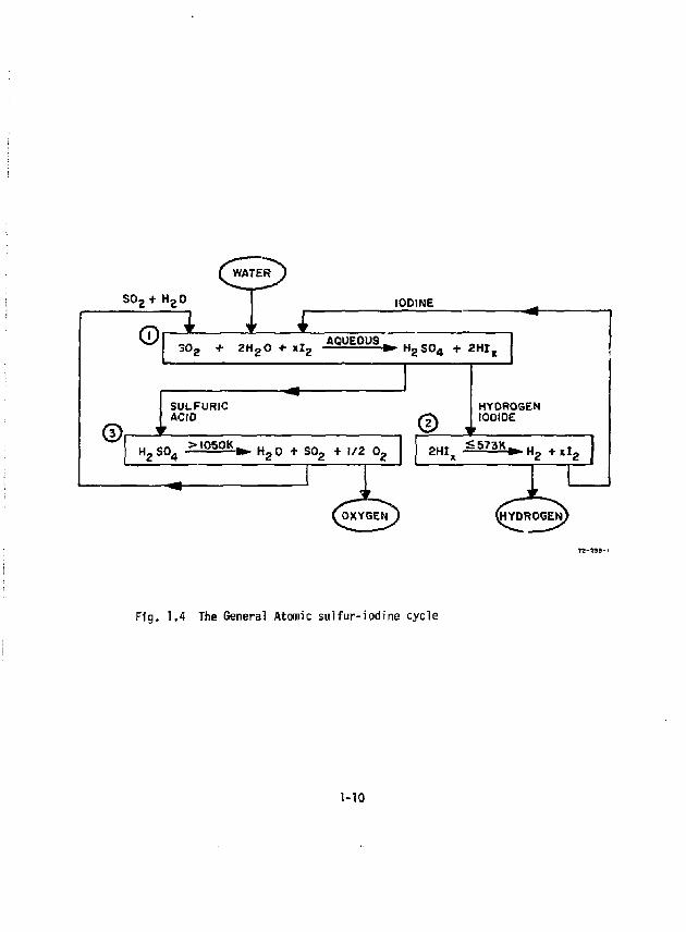
The therriochemical process uses General Atomic's sulfur-iodine cycl§. The net result of this cycle, as Fig. 1.4 illustrates, is the thermochemicai decomposition of water to make hydrogen and oxygen using only water as the feedstock. It is a pur« thermochemical cycle (without electrolysis) and is

1-5

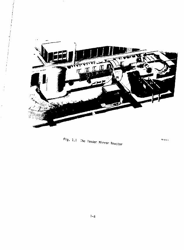
F f 9 - U The Tandem Mirror Reactor

1-6

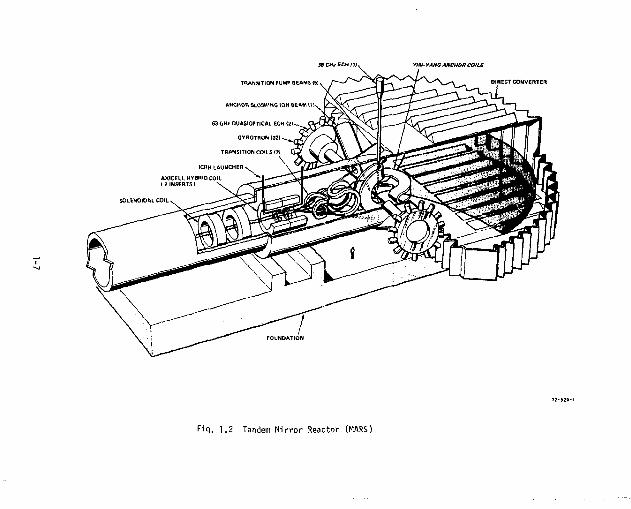
st-etiiECHfjf. y-w-y-wc ANCHOR cofis

TRANSITION PUMP BEAMS <5] ^

ANCHOR SLOSH'NG ION BEAM ( 1 ! v

63 GHt QUASIOPTICAL ECH (21-^

GVROTRON(32l-

TRANSITION COILS (2)

\ ICRH LAUNCHER \

DIRECT CONVERTER

SOLEN01DALCOIL s

FOUNDATION

Fiq. 1.2 Tandem Mirror Reactor (MARS)

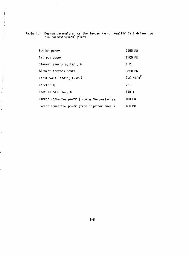
Table 1.1 Design parameters for the Tandem Mirror Reactor as a driver for the thermchemical plant

Fusion power 3500 MW Neutron power 2800 MW Blanket energy multip., M !.2 Blanket thermal power 3360 MM First wall loading (ave.) 2.0 MW/m 2

Raactor Q 25. Central cell length 150 m Direct convertor pover [from alpha particles) 700 MW Direct convertor power (from injector power) 140 MW

1-8

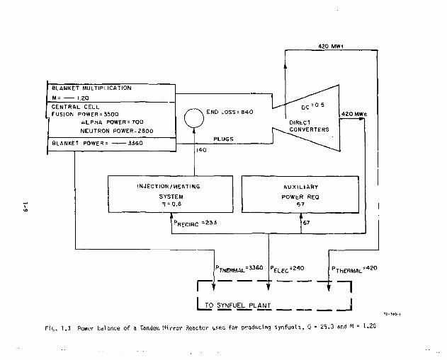
420 MWt

SWUEL_PLANT j

Fig, 1,3 Power balance of a Tandem Mirror Reactor u*ed for producing synfuels, Q = 25.0 and M = 1.:

^WATER^

S 0 2 + H E 0

O 1 IODINE

4 *. 3 0 2 + 2HgO + Xl 2

AQUEOUS. H 2 S 0 4 + 2 H I x

Q SULFURIC ACID

H 2 S 0 4

> l 0 5 0 K l » H gO + S 0 2 + 1/2 Oz

0 v HYDROGEN IODIDE

2HI. <573K * - H 2 + xlg

Fig. 1.4 The General Atomic sulfur-iodine cycle

1-10

described by the major reaction steps shown in Fig. 1,4. Major parts of the process are associated with separation and purification of the reaction products. For example, a critical aspect for the successful operation of the process is in the separation of the aqueous reaction products in reaction (]). Researchers at the General Atomic Company have solved this problem by using an excess of I,, which leeds to separation of the products into a lower density liquid phase, containing HoSO^ and HjO, and a higher density liquid phase containing HI, I, and H~0.

Reaction {2} shows the catalytic decomposition of HI, which is in the purified liquid form (50 atmj. Pure H~ is obtained by scrubbing out I 2 with H 20.

The equilibrium for reaction (3) lies to the right at temperatures above 1000 K, but catalysts or higher temperatures are needed to attain suffi­ciently rapid decomposition rates below 1250 K. Catalysts are available for this process, but careful consideration needs to be given to their costs versus effectiveness.

1.5 REACTOR BLANKET DESIGN* THE CANISTER BLANKET WITH THE JOULE-BOOSTED DECOMPOSER - OUR OPTION

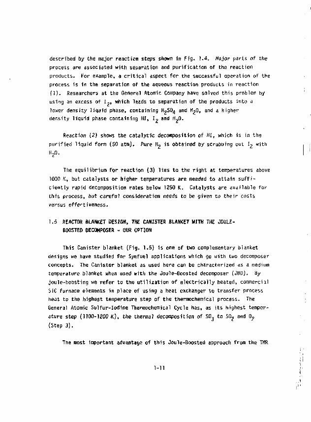
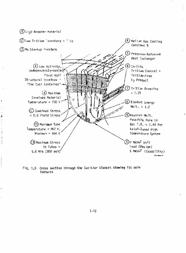
This Canister blanket (Fig, 1.5) is one of two complementary blanket designs we have studied for Synfuel applications which go with two decomposer concepts. The Canister blanket as used here can be characterized as a medium temperature blanket when used with the Joule-Boosted decomposer (JBD). By joule-boosting we refer to the utilization of electrically heated, commercial SiC furnace elements in place of using a heat exchanger to transfer process heat to the highest temperature step of the thermochemical process. The General Atomic Sulfur-Iodine Thermochemical Cycle has, as its highest temper­ature step (1100-1200 K ) , the thermal decomposition of S0 3 to S0 ? and Q?

(Step 3).

The most important advantage of this Joule-Boosted approach from the TMR

1-11

(pt-i^O Breeder Material

(2)Low Tritium 'nventory < 1 kg

(3)No Startup Problems

Low Activity, Independently-cooledf

First Wall Structural Envelope = "The Cool Container"-

\BJ Maximum Envelope Material

Temperature = 730 K'

(o) Combined Stress < 0.5 Yield Stress'

(jj) Maximum Tube Temperature = 962 K,

Minimum = 566 K

(jj) Maximum Stress in Tubes =

5.6 MPa (800 psi)

Helium Gas Cooling Constant Ti

Pressure-Balanced Heat Exchanger

C D In-Situ Tritium Control = Tritium-Free Hg Product

Tritium Breeding > 1.25

( D Blanket Energy Mult. s. I.?

©Neutron Mult. Possible Here to Get T.B. % 1.44 for Axial-Zoned High Temperature System

® 2 MW/m? Wall Load (Dfosign) 5 MW/m2 (Caoability)

Fig. 1.5 Cross section through the Canister blanket showing its main features

1-12

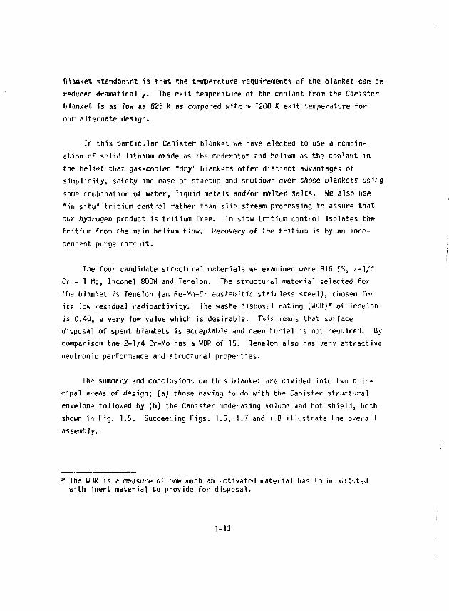
Blanket standpoint is that the temperature requirements of the blanket car. be reduced dramatically. The exit temperature of the coolant from the Carister blanket is as low as 825 K as compared with -v, 1200 K exit temperature for our alternate design.

In this particular Canister blanket we have elected to use a combin­ation o* sol id lithium oxide as the moderator and helium as the coolant in the belief that gas-cooled "dry" blankets offer distinct advantages of simplicity, safety and ease of startup and shutdown over those blankets using some combination of water, liquid metals and/or molten salts. We also use "in situ" tritium control rather than slip stream processing to assure that our hydrogen product is tritium free. In situ tritium control isolates the tritium from the main helium flow. Recovery of the tritium is by an inde­pendent purge cirruit.

The four candidate structural materials we examined were 316 SS, c-M^ Cr - 1 Mo, Inconel 800H and Tenelon. The structural material selected for the blanket is Tenelon (an Fe-Mn-Cr austem'tic stairless steel), chosen for its loh residual radioactivity- The waste disposal rating (WDR)* of Tenelon is 0.40, a very low value which is desirable. This means that surface disposal of spent blankets is acceptable and deep turial is not required. By comparison the 2-1/4 Cr-Mo has a WDR of 15. Tenelon also has very attractive neutronic performance and structural properties.

The summary and conclusions on this blanket are divided into two prin­cipal areas of design,- (a) those having to do with the Canister structural envelope followed by (b) the Canister moderating volume and hot shield, both shown in Fig. 1.5. Succeeding Figs. 1.6, 1.7 and i.8 illustrate the overall assembly.

* The WDfi is a measure of how much an actiyated material has to be diluted with inert material to provide for disposal.

1-13

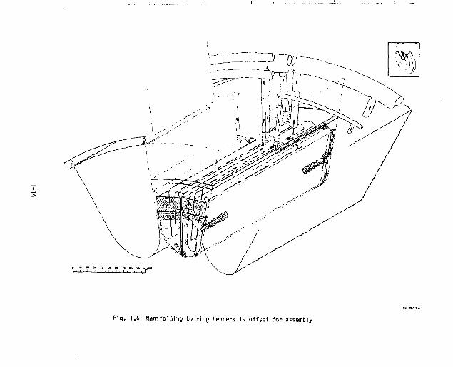
Fig, 1,6 Manifolding to ring headers is offset for assembly

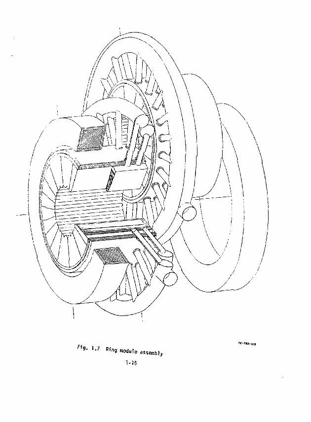
" 9 . 1.7 Rf n g module assembly

1-15

' i - n j - o , ,

V(EW R0TAT60 180»

100 l M 200 250 100 S5Q 400 490 CM 'J"'

Fig. 1.8 The ring module installation is straightforward - solenoids stay in place

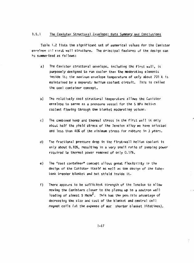
1.5,1 The Canister Structural Envelope: Data Summary and Conclusions

Table 1.2 lists the significant set of numerical values for the Canister envelope ?"•:'• Tir-it wall structure. The principal features of the design can ha summarized as follows:

a) The Canister structural envelope, including the first wall, is purposely designed to run cooler than the moderating elements inside it; the maximum envelope temperature of only about 731 K is maintained by a separate helium coolant circuit. This is called the cool container concept.

b) The relatively cool structural temperature allows the Canister envelope to serve as a pressure vessel for the 5 MPa helium coolant flowing through the blanket moderating volume

c) The combined hoop and thermal stress in the first wall is only about half the yield stress of the Tenelon alloy we have selected and less than 405» of the minimum stress for rupture in 3 years.

d) The fractional pressure drop in the first-wall helium coolant is only about 0.10%, resulting in a very small ratio of pumping power required to thermal power removed of only 0.173i.

e) The "cool container" concept allows great flexibility ir the design of the Canister itself as well as the design of the tube-bank breeder blanket and hot shield inside it.

f) There appears to be sufficient strength of the Tenelon to allow moving the Canisters closer to the plasma up to a neutron wall 2 loading of almost 5 MW/m . This has the possible advantage of decreasing the size and cost of the blanket and central cell magnet coils lit the expense of muc shorter blanket lifetimes).

1-17

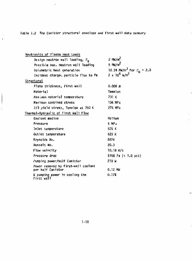
Table 1.2 The Canister structural envelope and first wall data summary

Neutronics of Plasma Heat Loads — — — — — — — ^ — — — .

Design neutron wall loading, r N 2 MW/itr Pcssible max. neutron wall loading 5 MW/m Volumetric heat, generation 18.34 MW/m for r„ = 2.0

A ? Incident charges particle flux to FH 2 x 10 W/m

Structural Plate thickness, f irst wall 0.006 m Material Tenelon Maximum material temperature 731 K Maximum combined stress 136 MPa 2/3 yield stress, Tenelon at 750 K 275 MPa

Thermal-Hydraulic of Fi rst Wall Flow Helium Coolant medium Helium

Pressure 5 MPJ Inlet temperature 525 K Outlet temperature 625 K Reynolds No. 5676 Nusselt No. 20.3 Flow velocity 10.18 m/s Pressure drop 5158 Pa {< 1.0 psi) Pumping power/half Canister 210 W Power removed by f per half Canister

irst-wall coolant 0.12 MW

% pumping power in cooling the 0.17% first wall

1-18

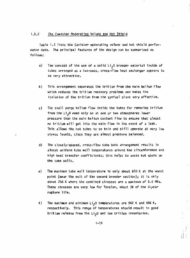
1.5.2 The Canister Moderating Volume and Hot Shield

Table 1.3 lists the Canister moderating volume and hot shield perfor­mance data. The principal features of the design can be summarized as follows:

a) The concept of the use of a solid Li z0 breeder material inside of tubes arranged as a two-pass, cross-flow heat exchanger appears to be very attractive.

b) This arrangement separates the tritium from the main helium flow which reduces the tritium recovery problems and makes the isolation of the tritium from the synfuel plant very effective.

c) The small purge helium flow inside the tubes for removing tritium from the Li ?0 need only be at one or two atmospheres lower pressure than the main helium coolant flow to ensure that almost no tritium will get into the main flow in the event of a leak. This allows the hot tubes to be thin and still operate at very low stress levels, since they are aTmost pressure balanced.

d) The closely-spaced, cross-flow tube bank arrangement results in almost uniform tube wall temperatures around the circumference and high heat transfer coefficients; this helps to avoid hot spots on the tube walls.

e) The maximum tube wall temperature is only about 810 K at the worst point (near the exit of the second breeder section); it is only about 758 K where the combined stresses are a maximum of 5.6 MPa. These stresses are very low for Tenelon, about 3% of the 3-yee.r rupture life.

f) The maximum and minimum Li 20 temperatures are 962 K and 666 K, respectively. This range of temperatures should result in good tritium release from the Li 20 and low tritium inventories.

1-19

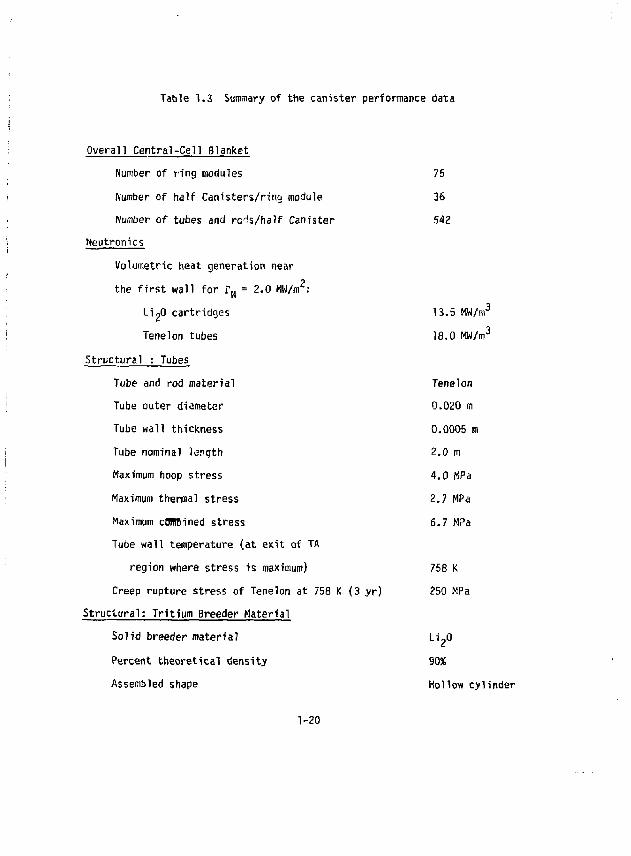
Table 1.3 Summary of the canister performance data

Overall Central-Cell Blanket Number of ring modules 75 Number of half Canisters/ring module 36 Number of tubes and rc^s/half Canister 542

Meutronics Volumetric heat generation near the first wall for r N = 2.0 MW/m2:

Li'20 cartridges 13.5 MW/m 3

Tenelon tubes 18.0 MW/m 3

Structural : Tubes Tube and rod material Tenelon Tube outer diameter 0.020 m Tube wall thickness 0.0005 m Tube nominal length 2.0 m Maximum hoop stress 4.0 MPa Maximum thermal stress 2.7 MPa Maximum cBTOined stress 6.7 MPa Tube wall temperature {at exit of TA

region where stress is maximum) 758 K Creep rupture stress of Tenelon at 758 K (3 yr) 250 MPa

Structural: Tritium Breeder Material Solid breeder material Li ?0 Percent theoretical density 90% Assembled shape Hollow cylinder

1-20

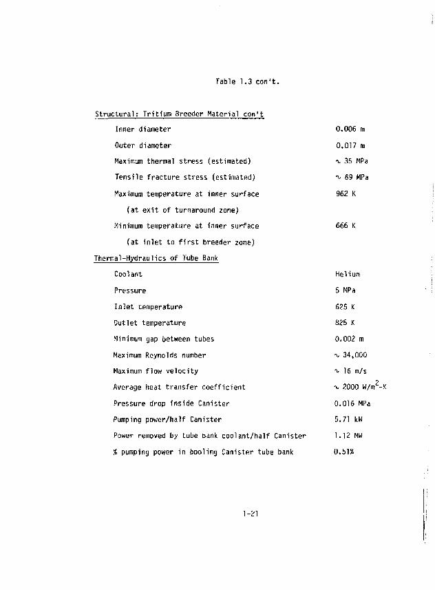
Table 1.3 con't.

Structural; Tritium Breeder Material con't Inner diameter 0.006 m Outer diameter 0.017 m Maximum thermal stress (estimated) ^ 35 MPa Tensile fracture stress (estimated) ^ 69 MPa Maximum temperature at inner surface 962 K

(at exit of turnaround zone) Minimum temperature at inner surface 666 K

(at inlet to first breeder zone) Thermal-Hydraulics of Tube Bank

Coolant Helium Pressure 5 MPa Inlet temperature 625 K Outlet temperature 825 K Minimum gap between tubes 0.002 m Maximum Reynolds number i. 34,000 Maximum flow velocity •*- 16 m/s Average heat transfer coefficient ^ 2000 W/m -K Pressure drop inside Canister 0.016 MPa Pumping power/half Canister 5.71 kW Power removed by tube bank coolant/half Canister 1.12 MW % pumping power in booling Canister tube bank 0.51%

1-21

g) The fractional pressure drop across the tube bank is only 0.3218, which results in a ratio of the pumping power required to the thermal power removed of only 0.51%.

h) A great deal of refinement and optimization of the tube bank design is possible, since same tailoring of the tube diameters and spacings can be used tc compens?*-; for the near-exponential decrease in the internal heat generation.

1.6 REACTOR BLANKET DESIGN, THE CANISTER/HIGH TEMPERATURE AXIALLY ZONED BLANKET WITH THE FLUIDIZED BED DECOMPOSER - OPTION 2

The Canister blanket discussed here is a high temperature design to be used in conjunction with the medium temperature design discussed in Section 1.5. This high temperature design does not breed tritium but instead relies upon the medium temperature design to provide the tritium breeding. The high temperature energy partition is accomplished by axially zoning the TMR into high and medium temperature zones as shown in Fig. 1.9. The required fraction of axial length for high temperature thermal energy involves a tradeoff between the fraction of high temperature energy supplied to the thermochemical process and the overall tritium breeding ratio.

Tritium breeding was excluded from the high temperature blanket to allow direct coupling with the 5 0 3 decomposer (1100 K) without concern for tritium contamination of the thermochemical process. An intermediate heat exchanger could be used to provide tritium isolation; however, this would increase maximum blanket temperature (from 1175 K to about 1375 K) to account for the necessary temperature differences in the heat exchanger. This was not considered to be an acceptable option at this stage of the study.

The primary advantage of providing high temperature thermal energy direct to the decomposer is the higher thermal energy utilization. The overall plant efficiency when using the direct-coupled fluidized bed decomposer is 43X as compared to 38% for the medium temperature blanket and

1-22

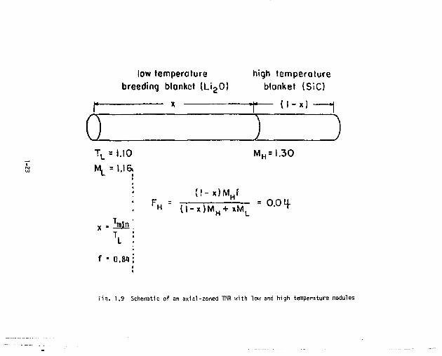
low temperature high temperature breeding blanket ( L i 2 0 ) blonket (SiC)

p x _^. ( | _ x ) ^

a )

\ = 1.10 M L = 1.16.

f • 0.81

M H = I . 30

{ ! - x ) M H f

l l - x ) M u + x M . = °'°^

Fiq. 1.9 Schematic of an axial-zoned TNR with low and high temperature modules

the Joule-Boosted decomposer. The primary disadvantage is the problem of finding materials with acceptable strength and chemical properties operating at -v. 1100 K.

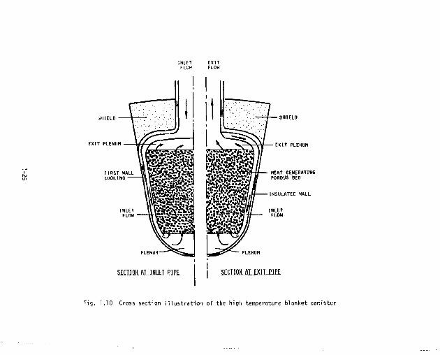
The design philosophy for the high temperature blanket is very similar to the medium temperature blanket. A gas-cooled Canister design was selected as shown in Fig. 1.10. It is intended to fit into the same modular structure shown in Figs. 1.6, 1.7 and 1.8.

1.6.1 The Canister Structural Envelope: Data Summary and Conclusions

Table 1.4 lists performance data for the Canister envelope and first wall structure. The principal features of the design can be summarized as follows:

a) The Canister wall is cooled by helium entering at 750 K and exiting at 800 K. The maximum wall temperature is 835 K and occurs at the "nose" of the Canister.

b) The relatively cool Canister wall allows the Canister to serve as the pressure vessel and contain the system pressure (50 atm).

c) The arrangement of Canisters is such that they are mutually self supporting. The stresses of concern are primarily thermal stresses and hoop stresses in the nose region. The hoop stress for a 6-mm-thick wall is a reasonable 110 HPa (13000 psi).

d) The pressure drop through the 3 mm coolant channel is 0.56 atm.

1.6.; The Canister High Temperature Region

Table 1,5 lists performance data for the high temperature region. The principal features of the design are summarized as follows:

1-24

INLET FLOW

EXIT FLOW

EXIT PLENUM

FIRST WALL COOLING

INLET FLOW

SECIiQH.AUNLET PIPE

EXIT PLENUM

HEAT GENERATING POROUS BED

INSULATED WALL

Fig. 1.10 Cross section illustration of the high temperature blanket canister

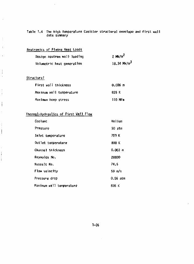
Table 1.4 The high temperature Canister structural envelope and first wall data summary

Neutronics of Plasma Heat Loads Design neutron wall loading Volumetric heat generation 18.34 MU/nr Design neutron wall loading 2 MW/m z

Structural First wall thickness 0.006 m Maximum wall temperature 835 K Maximum hoop stress 110 HPa

Thermal-Hydraulics of First Wall Flow Coolant Helium Pressure 50 atm Inlet temperature 750 K Outlet temperature 800 K Channel thickness 0,003 m Reynolds No. 26800 Nusselt No. 74.5 Flow velocity 59 m/s Pressure drop 0.56 atm Maximum wall temperature 835 K

1-26

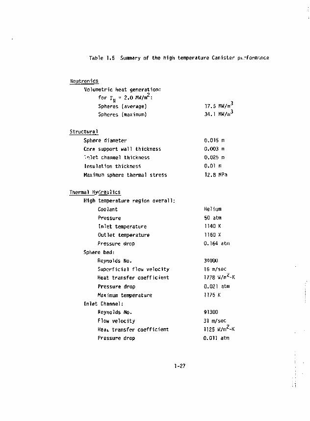
Table 1.5 Summary of the high temperature Canister pt.-form-.nce

Neutronics Volumetric heat generation:

for r„ = 2.0 MW/m 2: N

Spheres (average) Spheres (maximum)

17.5 MW/mJ

34.1 MW/m3

Structural Sphere diameter 0.015 m Core support wall thickness 0.003 m '• let channel thickness 0.02b m Insulation thickness 0.01 m Maximum sphere thermal stress 12.8 MPa

Thermal Hydraulics High temperature region overall;

Coolant Helium Pressure 50 atm Inlet temperature 1140 K Outlet temperature 1160 X Pressure drop 0.164 atm

Sphere bed: Reynolds No. 34000 Superficial flow velocity 16 m/sec Heat transfer coefficient 1778 W/m 2-K Pressure drop 0.021 atm Maximum temperature 1175 K

Inlet Channel: Reynolds No. 91300 Flow velocity 31 m/sec Heai, transfer coefficient 1125 W/m 2-K Pressure drop 0.011 atm

1-27

a) The non-breeding high temperature neutron moderating region is considered to be a porous bed of 15 mm diameter silicon carbide spheres. (While spheres were used for the current design, other forms could possibly be used to advantage.)

b) The high temperature region is separated from the Canister wall by the first wall cooling channel, an insulated wall, and the inlet flow channel. The insulated wall reduces the heat loss from the high temperature inlet stream to the first wall coolant.

c) The total energy available a.t high temperature is 84%. The remaining 16% is lost to the first wall coolant (12%) and to the shield (45!).

d) The high temperature region operate;, at 50 atm and is pressure balanced with the first wall coolant. The high temperature structure need only be se?f supporting.

e) The pressure drop of the primary helium flow through the entire Canister is 0.17 atm.

f) The maximum structural temperature is estimated to be 117S K.

1.6.3 General Conclusions

Since the high temperature Canister blanket must operated in conjunc­tion with the medium temperature blanket and synfuel plant, the following general conclusions are made:

a) Axial zoning is an attractive option for a fusion reactor designed to produce high temperature heat for a synfuel plant. The physical separation of the high temperature energy recovery and tritium breeding has the virtue of blanket module simplicity.

1-28

b) Since the high temperature blanket does not breed tritium, the medium temperature blanket must be a high breeder for the overall breeding ratio to be 1.1. This would require the use of a neutror multiplier to enh.nce the tritium breeding ratio to ^ 1.4. Of the options considered thus far, the most promising appears to be a Li^n design with a lead-zirconate multiplier.

c) Absolute helium pressure of aoout 50 atm is necessary to maintain acceptable pressure drop. The system pressure is contained by the specially cooled first wall (pressure boundary) and helium transport piping. The heat exchanger tubes of the fluidized bed decomposer must also contain system pressure and at high temperature.

d) The direct-coupled high temperature blanket concept presented here offers a high thermal efficiency for hydrogen production. The success of realizing this efficiency will require a high breeding medium temperature blanket and a successful heat exchanger design for the SO, decomposer.

1.7 "IN SITU" TRITTUM CONTROL - PRODUCING A TRITIUM-FREE HYDROGEN PLANT

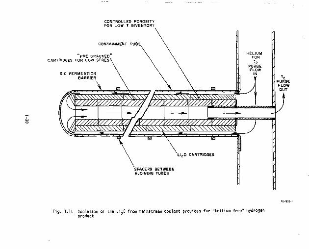
We propose to fill the tubes shown in the Canister blanket module of Fig. 1.5 with half washers or split rings of IU°- ^ n e advantage of this shape is that the LioO cartrides are "pre-cracked" axially and radially so that thermal stress problems can be minimized. The sub-assembly is thus a long tube filled with half washers or split rings, as shown in Fig. 1.11. These filled tubes are assembled in the Canister normal to the helium coolant flow. The tubes are rigidly mounted in a tube sheet at one end of the blanket only, to allow for thermal expansion.

Purge flow helium is introduced into the annular gap around the outside of the Li ?0 and returns through the tuba center for tritium removal. The purge flow quantity may be less than ~\% of the total flow. This circuit is

1-29

CONTROLLED POROSITY FOR LOW T INVENTORY

CONTAINMENT TUBE

PRE CRACKED CARTRIDGES FOR LOW STRESS

SiC PERMEATION BARRIER

SPACERS BETWEEN AJOINING TUBES

Fig. 1.11 Isolat ion of the LipO from mainstream coolant provides for " t r i t ium- f ree" hydrogen product

completely separate from the main stream helium. The purge helium pressure is adjusted to be slightly less than the main flow helium pressure. The assembly of tubes are mutually supporting, separated by helically wound wires or by staggered rings.

The tubes must have low permeation for tritium since the main reason the tubes are used is to minimize the tritium release from the LigO to the main helium coolant stream. The other reason for placing the t^O in a tube container is to protect the Li 20 from possible disintegration due to the high velocity helium flow or chemical attack by trace impurities in the main helium flow.

The practical metals, such as our design choice of Tenelon, for use as Canister material or high temperature heat exchanger:: are too permeable to tritium to act as significant barriers. A thin coating (100 k"n) of sili­conized SiC on the inside or the outside of each tube would greatly reduce the permeation of tritium into the main helium coolant. At the operating temperature it can be postulated that the coating is self healing. It is calculated that only 900 std cc per day would permeate at 950 K into the main coolant. By slip stream processing 10" of the main helium coolant for tritium removal following the in situ control, the amount permeating into our intermediate process steam cycle, for example, would be only 1 std cc/day. This assumes another permeation barrier such as alumina is used on the tubes in the intermediate heat exchanger.

1.8 PROGRESS IN NEUTR0MCS

In addition to the development of the neutronics data base r.acessary to support the present design of both the Joule-Boosted and the two-zone blankets, neutronics results have been obtained which have more general significance.

The combined use of a high density solid lead neutron multiplier together with a Li ?0 breeding region makes a very versatile and synergistic

1-31

combination. Such a combination is very attractive in achieving acceptable tritium breeding rates with relatively thin olankets, very high tritium breeding rates (for auxiliary tritium supplies), or increasing energy deposi­tion in a hot shield. Although lead zirconate (Zr-Pb,) has been used in the present work, some other solid lead compound might also be used if ZrgPb3 is unacceptable for some reason.

The presence of a high Z material immediately uehind the first wall has been shown to be an effective method for reducing the first wall power density for a given first wall loading. This result is produced by prefer­ential absorption of gamma rays in the high Z material.

Tenelon has been shown to be a very attractive structural material. The combination of impressive neutronics performance together with high tempera­ture materials properties is impressive and perhaps unique among structural materials that have been studied thus far.

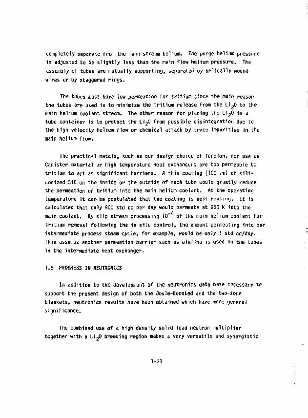
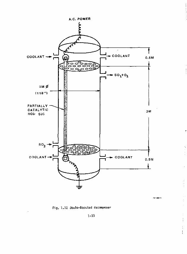
1.9 THE JOULE-BOOSTED DECOMPOSER

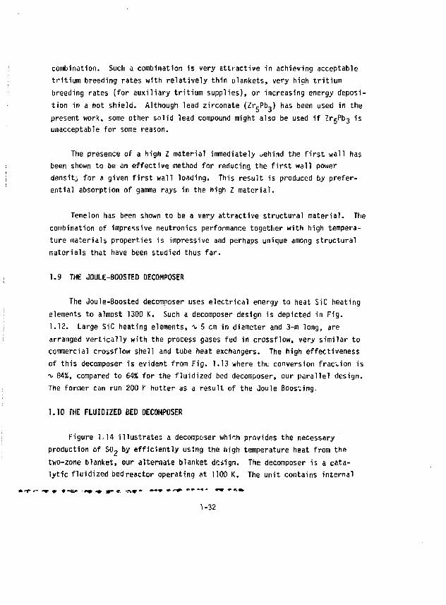
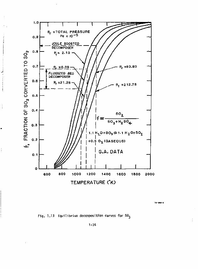
The Joule-Boosted decomposer uses electrical energy to heat SiC heating elements to almost 1300 K. Such a decomposer design is depicted in Fig. 1.12. Large SiC heating elements, ^ 5 cm in diameter and 3-m long, are arranged vertically with the process gases fed in crossflow, very similar to commercial crossflow shell and tube heat exchangers. The high effectiveness of this decomposer is evident from Fig. 1.13 where thb conversion fraction is i. 84%, compared to 64% for the fluidized bed decomposer, our parallel design. The former can run 200 Y hotter as a result of the Joule Boosting.

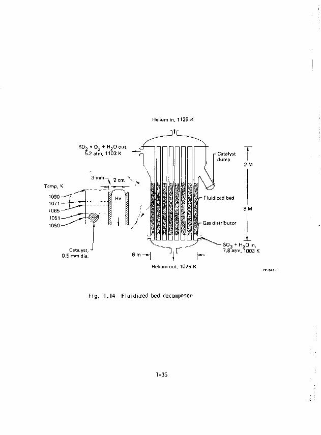
1.10 THE FLUIDIZED BED DECOMPOSER

Figure 1,14 illustrates a decomposer whi^h provides the necessary production of SO- by efficiently using the high temperature heat from the two-zone blanket, our alternate blanket design. The decomposer is a cata­lytic fluidized bed reactor operating at 1100 K. The unit contains internal

1-32

A.C. POWER

COOLANT

3M 0 ( 1 1 8 " )

PARTIALLY CATALYTIC ROD SiC

SO,

COOLANT -

F ig . 1.12 Joule-Boosted decomposer

1-33

1.0

600 BOO 1000 1200 1400 1600 1800 2000

TEMPERATURE (°K)

Fig. 1.13 Equilibrium decomposition curves for S03

1-34

Helium in, 1125 K

Temp, K

1090-1071 1065 1051 1050

S 0 2 + 0 2 + H 2 0 out, 5.2 atm, 1103 K Catalyst

dump

Fluidized bed

s i r Gas distributor

T 2 M

8 M

Catalyst 0.5 mm dia 6 m — | I K-

Helium out, 1075 K

S 0 3 + H ,0 in, 7.8 atm, 1003 K

Fig. 1.14 Fluidized bed decomposer

1-35

heat exchanger tubes to provide the heat for the highly eodotnermic SO, decomposition, A 65% conversion can be obtained using a CuO catalyst, if sulfation of the substrate does not became a problem around 1050 K, or a more expensive platinum catalyst on a titania support can be used if sulfation is a serious pro^'em.

1.11 MATERIALS

For the selection of materials in the corrosive atmosphere of tYis GA cycle four equations describe the four sections of the thermochemical plant:

Section I S0 Z + xl ? + HgO £H 2S0 4{1) + 2HIO) Section II H 2 S 0 4 + H 20 + S 0 2 + 1/2 0 2

Section III 2HI X - 2HI +(x-l)I2

Section IV 2HI * H? + l^

An extensive materials testing program be carried out by 6A during the process development effort. Since sulfuric acid is common to other thermo-cheraical cycles and is industrially significant, other workers have exten­sively investigated materials for the H^SO^-H^O system which we have taken advantage of in choosing materials-

A great deal of data exists on corrosion in iodine syst&ns. Table 1.6 presents a summary of the test results. Early results indicated that niobium was an additional material impervious to attack by the HI-I,-H20 solutions typical of the main solution reactor, but the most recent work regarding the effect of the H~S0- upon the system questions the use of niobium in this portion of the process. Tantalum can be substituted for the niobium, at higher cost, but this has not been done in the present equipment design.

Although glass-lined steel is an ideal material for use with the HI-I2-HpO system, it is unavailable in the equipment s?2es required for the TMR-powered plant. Fluorocarbon-lined steel performs the same function and is available in the desired equipment sizes.

1-36

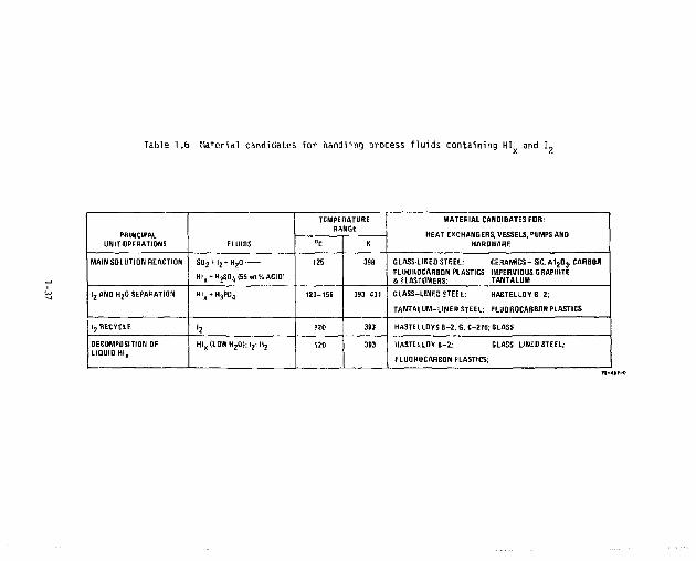
Table 1.6 Material candidates for handling process fluids containing HI and I

PRINCIPAL UNIT OPERATIONS FLUIDS

TEMPERATURE RANGE

MATERIAL CANDIDATES FOR:

HEAT EXCHANGERS, VESSELS, PUMPS AND HARDWARE

PRINCIPAL UNIT OPERATIONS FLUIDS °C K

MATERIAL CANDIDATES FOR:

HEAT EXCHANGERS, VESSELS, PUMPS AND HARDWARE

MAIN SOLUTION REACTION SOj +l 2-t H 20

HI , + H2SQ4(5S««t%AC10l

125 398 GLASS-LINED STEEL. CERAMICS - SiC. A1 2 0 3 . CARBON FLUOROCARBON PLASTICS IMPERVIOUS GRAPHITE a ELASTOMERS: TANTALUM

l 2 AND H 20 SEPARATION H I^H jPO, 120-158 393-131 GLASS-LINED STEEL: HASTELLOV B-2;

TANTALUM-LINED STEEL: FLUOROCARBON PLASTICS

l 2 RECYCLE '2 120 393 HASTEl LOVS B-2, G, C-276: GLASS

DECOMPOSITION OF I,QUID HI ,

Hl x ( lO«VH 2 0); l z ; H 2 120 393 HASTEllDV B-2: GLASS-LINED STEEL;

FlUOROCARBON PLASTICS:

Material selection for Sections III and IV is similar to that selected for Sections I and II. The information in Table 1.7 is applicable to the sulphuric acid section of the process.

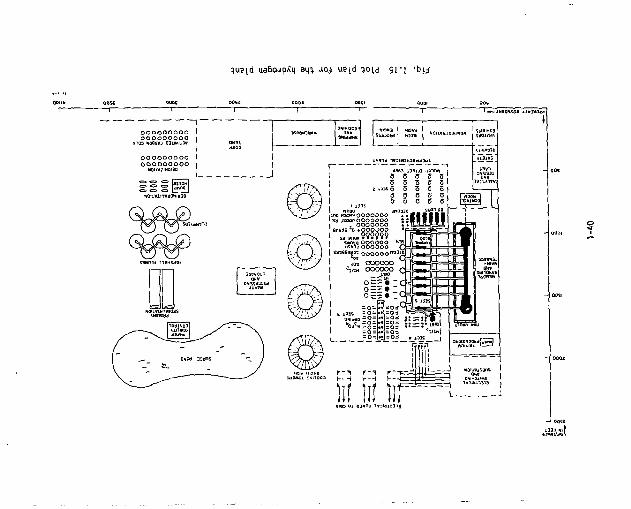
1.1E A PLOT PiM FOR THE HYDROGEN PLANT

An artist's conceptual drawing of the plot plan as given in last year's report is shown in Fig. 1.15. Changes in this year's design did not materially affect space requirements, so this plot plan still gives a rough idea of the approximate land area and relative sizes of the TMR nuclear island, turbine generator, steam generator and process he.t exchanger building, as well as the rest of the chemical plant. He conclude from the plot plan that this plant is quite compact, and raises no new issues regarding heat transport distances, safety, etc.

1.13 PROGRESS IN MEETING THE HIGH TEMPERATURE REQUIREMENTS OF THE PROCESS

Roughly 22-25% of the energy demand of the thermochemical plant is at high temperature (> 1050 K) and is required to decompose SO^ to S0~, which is the final step .n the HjSO^ decomposition. The remaining energy requirement is at much lower temperature.

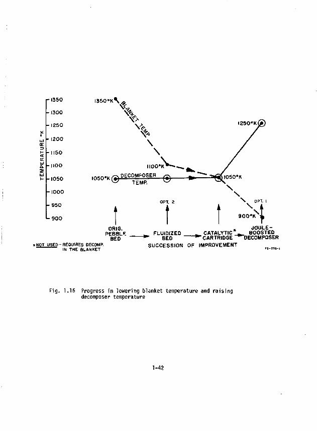
Our introduction of the Joule-Boosted decomposer concept is an important system improvement in Fusion/Synfuels compatibility allowing very high 50, decomposition temperatures ( 1Z50 K) to be provided electrically but significantly relaxing temperature demands on the reactor blanket to as low as 82b K exit gas temperature. This Joule Boosting works by using the unique high voltage direct current output from the TMR plus some additional elec­tricity that is thermally derived from the blanket. The electric power produces high temperatures using electrical heating elements right in the decomposer itself rather than del'! ering high temperature process heat.

A fluidized bed decomposer, which we also introduced during the course of our study, requires the use of higher temperature t 1200 K blankets.

1-38

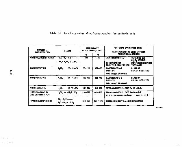
Table 1.7 Candidate materials-of-construction for sulfuric acid

PRINCIPAL UNIT OPERATION FLUIDS

APPROXIMATE FLUID TEMPERATURES

MATERIAL CANDIDATES FOR:

HEAT EXCHANGERS. VESSELS. PUMPS AND OTHER HARDWARE

PRINCIPAL UNIT OPERATION FLUIDS

°C °K

MATERIAL CANDIDATES FOR:

HEAT EXCHANGERS. VESSELS. PUMPS AND OTHER HARDWARE

MAIN SOLUTION REACTION S D 2 H 2 * H 2 0

Hl x *H 2 S0 4 <S5«wKI

125 39) GL>1SS-LINED STEEL; CERAMICS-SC, A 1 z 0 3 . CARBON;

FLUOROCARBON IMPERVIOUS GRAPHITE PLASTICS A ELASTOMERS; TANTALUM

CONCENTRATION H 2 S0 4 65-6SwtK SS-1SD 368-423 HASTELLOVSB-2 GLASS OR ORC-27E BRICK-LINED STEEL IMPERVIOUS GRAPHITE

CONCENTRATION HjSO,, 65-75 wl% 150-180 «3-453 HASTELLOVSB-2 GLASS OR ORC-276 BRICK-LINED STEEL IMPERVIOUS GRAPHITE

CONCENTRATION HjSfl, 75-9«wl% 1M-»20 •,53-693 BRICK-LINED STEEL;CAST F f - H ntSSi

VAPOR FORMATION AND DECOMPOSITION

H 2S0 4 — - H 2 0 t S0 3 330-600 603-873 BRICK-LINED STEEL; CAST Ft-14 wt SSi SILICIDE COATINGS ON STEEL; HASTELLOY G

VAPOR DECOMPOSITION HjO+SOj + 1/2 0 2

500-850 173-1123 INCOLOY 8D0H WITH ALUMINIDE COATING

T f - U M

}uBi<i U3fiojip/CM 3q} JOJ- u»[d *oid 9L'l "bij

DDS(

1 -jMTCNncte j i * j - fO*d

Jassssss ooooooooo ooooooooo

NDUVZINOISO

XN«1d l*3IH3«30nW3Hi

a 5 a 5

on BO d l*Q33Q ,jfK3 W O N * OOOOOOO My iEOOO OOOOOOO

, OGOOOOO annas 'o »00Oi>O0

0 0 0 0 0 0 ~Stftiia QOOOOO HS*ii OOOOOO

4W3 133*J3-lllr«

in in jir

The fluidized bed is also a significant system improvement in reducing blanket temperatures compared to its pebble bed predecessor that started our study. Figure 1.16 illustrates very vividly how we have been able to reduce blanket temperatures using fluidized bed or Joule Boosting.

1.14 HATCHING POWER AND TEMPERATURE DEMANDS - PERFORMANCE AND EFFICIENCY EVALUATIONS FOR THE JOULE-BOOSTED DECOMPOSER

1.14.1 Option 1

In order to satisfy the interfacing requirements, the Tandem Mirror Reactor (TMR) interface must be designed to supply all the electrical and thermal power demands of the thermochemical plant (TCP) after satisfying all the TMR internal and auxiliary demands. In addition, the TCP thermal power demands must be supplied to each section of the synfuel plant at the correct temperatures. The heat exchangers, steam generators and power plants which comprise the actual interface are shown on Fig. 1.17 in greatly simplified form for the Joule-Goosted decomposer (JBD) concept.

A straightforward procedure has been presented for performing the inter­face power and temperature matching between the TMR and the thermochemical plant (TCP) for preliminary design purposes. For the Joule-Boosted decom­poser fJBD) concept, an overall TCP efti-iency of about 30% is predicted for the reference case (with a steam power plant efficiency of 35%). Improve­ments in the thermochemical plant which reduce the thermal demand by 100 kJ./mole H„ and the electrical demand by 20 kJ /mole H~ can raise the TCP efficiency to about 36% (using the improved estimate of the steam power plant efficiency of 38%).

This TCP efficiency appears to be achievable with remarkably low helium coolant temperatures compared to most other processes for synthetic H 2

production. The helium exiting the blanket and direct converters need only be at about 825 K, while the helium exiting the first wall need only be at about 625 K. This should lead to a v&ry credible and cost-effective synfuel plant.

1-41

2£ a UJ = > 1-

-1350

-1300

-1250

-1200

-1150

I 3 5 0 ° K \ A

\ \

EM

PE

R/

-1100

-1050

-1000

I I O O ' K * - - . ^

. „ , - . . . . ^ DECOMf-OSER ~ t *"** —fjfno?0* r-

-1100

-1050

-1000

^ TEMP. ^ t

\

- 9 5 0

- 9 0 0

OPT. 2

| t ! ORIG.

PEBBLE ^ . FLUIDIZEO BED ^ BED

^ CATALYTIC^ •" CARTRIDGE

NOT USED-REQUIRES OECOMP. SUCCESSION IN THE BLANKET

OF IMPROVEMENT

1250'K

\ OPT. I \ i 900*K L

JOULE-BOOSTED

DECOMPOSER

Fig. 1.16 Progress in lowering blanket temperature and raising decomposer temperature

1-42

3360 M W t n

TMR REACTOR BLANKET

0=25

1401 MW

INJECT.

420 MW, i l

,=0.6

F i g . 1.17 S i m p l i f i e d energy balance - TMR/Synfuels fo r the Ooule-i)oosted decomposer concept

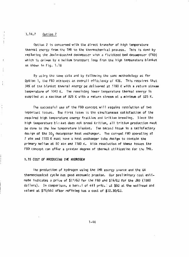
1.14.2 Option 2

Option 2 is concerned with the direct transfer of high temperature thermal energy from the TMR to the ttiermochemical process. This is done by replacing the Joule-Boosted decomposer with a fluidized bed decomposer (FBD) which is driven by a helium transport loop from the high temperature blanket as shown in Fig. 1.18

By using the same data and by following the same methodology as for Option 1, the FBD achieves an overall efficiency of 43%, This requires that 34% of the blanket thermal energy be delivered at 7160 K with a return stream temperature of 1040 K. The remaining lower temperature thermal energy is supplied at a maximum of 825 K with a return stream at a minimum of 525 K.

The successful use of the FBD concept will require resolution of two important issues. The first issue is the simultaneous satisfaction of the required high temperature energy fraction and tritium breeding. Since the high temperature bl?:,ket does not breed tritium, all tritium production must be done in the low temperature blanket. The second issue is a satisfactory design of the SO, decomposer heat exchanger. The current F80 operating at 7 atm and 1100 K must have a heat exchanger tube design to contain the primary helium at 50 atm and 1160 K. With resolution of these issues the FBD concept can offer a greater degree of thermal utilization for the TMR.

1.15 COST OF PRODUCING THE HYDROGEN

The production of hydrogen using the TMR energy source and the GA thermochemical cycle has good economic promise. Our preliminary cost esti­mate indicates a price of $l'/fiJ for the FBD and $15/GJ for the JBO (1980 dollars). In comparison, a b a n d of oil prict,.: at $50 at the wellhead and valued at f75/bbl after refining has a cost of $12.30/GJ.

1-44

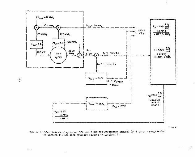
Fig. 1.18 Power balance diagram for the Joule-Boosted decomposer concept (with vapor recompression in Section III and some pressure staging in Section 11)

1.76 CHEMICAL PLANT OPERATIONAL DEPENDABILITY

With an appropriate degree of process unit redundancy that we have included, we can predict a high, combined TMR/chemical plant availability of v 74%, and this figure is included in our cost figures for the hydrogen produced.

1 .17 PROBLEM ARiTAS

Blanket design remains er, area of principal concern out is progressing well. Even with Joule Boosting or fluidized bed decomposers relaxing the temperature demands of the blanket, the design is difficult because of the myriad demands the blanket must satisfy. Much more attention is needed here. This concern is true for all blankets—for synfuels, for electricity, for co-generation, for hybrids. We feel that we have converged on a highly effective design approach using the non-flowing lithium-oxide blanket module with helium as a coolant. The module shows strong promise of being functional over a range of temperatures useful for synfuel production for electrical power production, or both.

In the chemical plant we wish to make substantial improvements in the HI separation and purification. This process requires a large amount cf power and has high capital costs (•>- 1/3 of the chemical plant).

The fluidized bed decomposer also needs additional design development for its high temperature and pressure service in a hostile chemical environ­ment.

1.18 RECOMMENDATIONS FOR FURTHER STUDY

Our analytical strdies have been very fruitful and produced innovative ideas and technical crntributions that help to lend good credibility to the Fiision/Synfuel tie. he recommer.' that the conceptual design for the reactor and chemical plant components continue to be refined and that an experi-

1-46

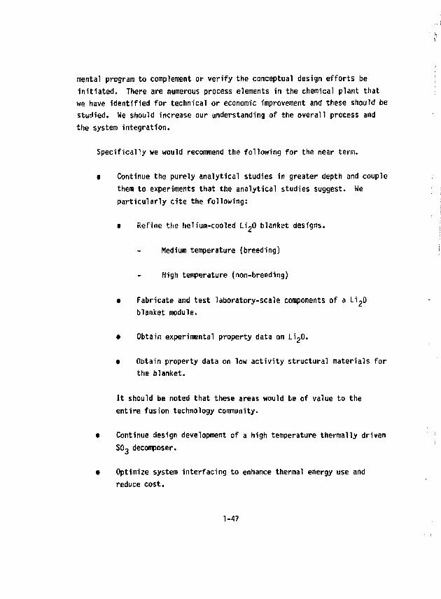
mental program to complement or verify the conceptual design efforts be initiated. There are numerous process elements in the chemical plant that we have identified for technical or economic improvement and these should be studied. We should increase our understanding of the overall process and the system integration.

Specifically we would recommend the following for the near term.

• Continue the purely analytical studies in greater depth and couple them to experiments that the analytical studies suggest. We particularly cite the following:

• Refine the helium-cooled LigO blanket designs.

Medium temperature (breeding)

High temperature (non-breeding)

• Fabricate and test laboratory-scale components of a Li 20 blanket module.

• Obtain experimental property data on Li^O.

• Obtain property data on low activity structural materials for the blanket.

It should be noted that these areas would be of value to the entire fusion technology community.

• Continue design development of a high temperature thermally driven SOo decomposer.

• Optimize system interfacing to enhance thermal energy use and reduce cost.

1-47

SECTION 2 MOTIVATION FOR THE STUDY

Contributor: R. W. Werner

TABLE OF CONTENTS Section Page 2.0 MOTIVATION FOR THE STUDY 2-1

LIST OF FIGURES Figure Page 2.1 U.S. energy flow - 1979 2-2 2.2 Contribution of various energy sources 2-4

2.0 MOTIVATION FOR THE STUM

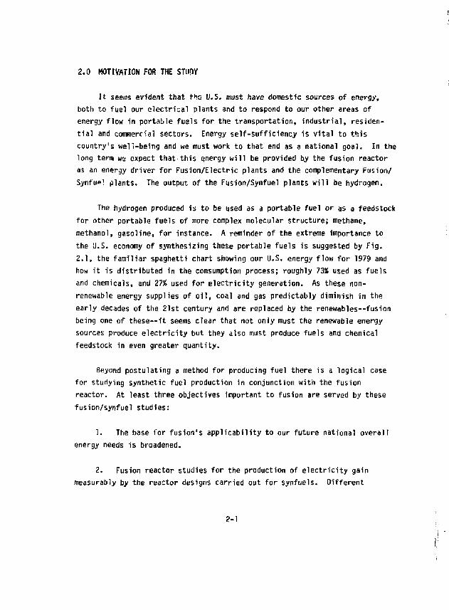
It seems evident that the- U.S. must have domestic sources of energy, both to fuel our electrical plants and to respond to our other areas of energy flow in portable fuels for the transportation, industrial, residen­tial and commercial sectors. Energy self-sufficiency is vital to this country's well-being and we must work to that end as a national goal. In the long term we expect that this energy will be provided by the fusion reactor as an energy driver for Fusion/Electric plants and the complementary Fusion/ Synfuel plants. The output of the Fusion/Synfuel plants will be hydrogen.

The hydrogen produced is to be used as a portable fuel or as a feedstock for other portable fuels of more complex molecular structure; methane, methanol, gasoline, for instance. A reminder of the extreme importance to the U.S. economy of synthesizing these portable fuels is suggested by Fig. 2.1, the familiar spaghetti chart showing our U.S. energy flow for 1979 and how it is distributed in the consumption process; roughly 7356 used as fuels and chemicals, and 27i£ used for electricity generation. As these non­renewable energy supplies of oil, coal and gas predictably diminish in the early decades of the 21st century and are replaced by the renewables—fusion being one of these—it seems clear that not only must the renewable energy sources produce electricity but they also must produce fuels and chemical feedstock in even greater quantity.

Beyond postulating a method for producing fuel there is a logical case for studying synthetic fuel production in conjunction with the fusion reactor. At least three objectives important to fusion are served by these fusion/synfuel studies:

1. The base for fusion's applicability to our future national overall energy needs is broadened.

2. Fusion reactor studies for the production of electricity gain measurably by the reactor designs carried out for synfuels. Different

2-1

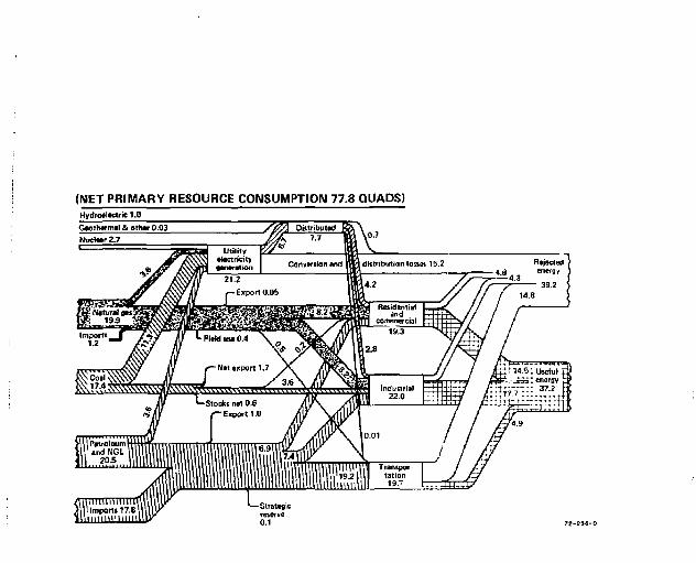
(NET PRIMARY RESOURCE CONSUMPTION 77.8 QUADS) Hytfrotltctricl.O

G t o t h f mil & othtr 0.03 NacHW 2.7

scientific disciplines become involved. Different industrial partnpr<; become aware of fusion.

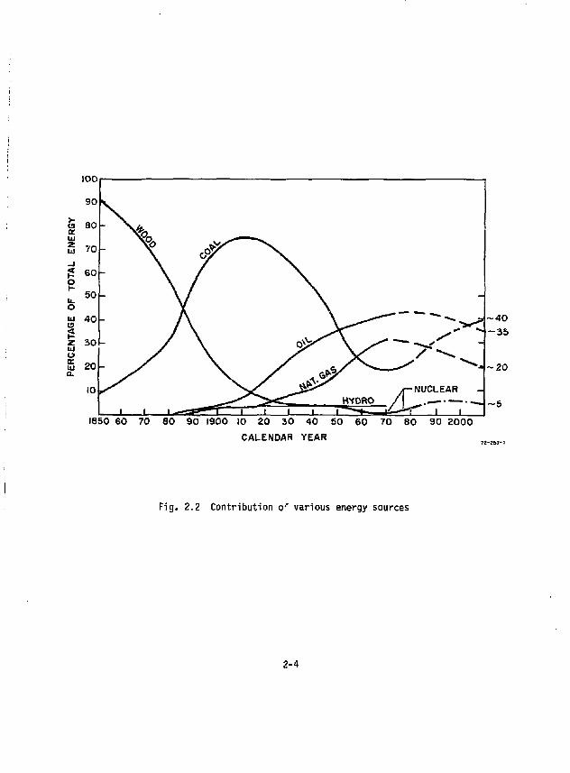
3. The timing of fusion's availability and the need for synfuels coincide. At"-Jt the time when fusion energy sources are on the threshold of commercial reality, synthetic fuels will be needed to bolster the waning supplies of the exhaustibles. Figure 2.2 illustrates the rise and fall of our various exhaustible energy sources starting with wood from 1850 up through the 2000's. Somewhere around 2010 or perhaps a decade thereafter tl ,re is a high probability of an energy shortfall and it is then that fusion must begin to be commercialized using the inexhaustib'les.

2-3

HYDRO /-NUCLEAR

~ 4 0 - 3 5

- 2 0

1650 60 70 SO 90 1900 IO 20 30 40 SO 60 70 80 90 2000 CALENDAR YEAR

Fig. 2.2 Contr ibut ion of various energy sources

2-4

SECTION 3 THE TANDEM MIRROR REACTOR AND ITS PHYSICS

Contributors: T. H. Zerguini and F. L. Ribe

TABLE OF CONTENTS Section Page 3.1 GENERAL DESCRIPTION OF THE REACTOR AND ITS PHYSICS . . 3-1 3.2 THE PLASMA MODELING COOE . 3-S

3.2.1 General Description of the Plasma Model . 3-8 3.2.2 Input and Output Variables . 3-8 3.2.3 General Description of the TMRBAR Code . 3-n

3.3 COMPUTED TANDEM MIRROR PARAMETERS . . 3-14 APPENDIX 3.1 . 3-19 REFERENCES . 3-30

l

LIST Of TABLES Tables page 3.1 TMR parameters for coupling to a plant using Ppus =

3500 Hwf and iy = 5 MW/m2 3-16

LIST Of FIGURES Figures Page 3.1 Tandem Mirror Reactor {MARS) 3-2 3.2 Comparison of A-cell and axicell magnet set

configurations 3-3 3.3 Axicell (MARS) magnetic field, ambipolar potential and

total density along axis 3-5 3.4 Profile of electron (a) and ion (b) densities within

the end cell regions of an axicell operated TMR 3-7 3.5 TMRBAR program flow chart 3-15 3.6 Power balance of an electricity producing Tandem

Mirrtr Reactor plant . . . . . . . . . . 3-18

ii

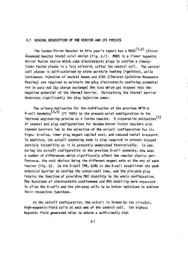
3.1 GENERAL DESCRIPTION OF THE REACTOR AND ITS PHYSICS

The Tandem Mirror Reactor in this year's report has a MARS1 ' ' (Mirror Advanced Reactor Study) axial design (Fig. 3.1). MARS is a linear magnetic mirror fusion device which uses electrostatic plugs to confine a steady-state fusion plasma in a long solenoid, called the central cell. The central cell plasma is self-sustained by alpha particle heating (ignition), while continuous injection of neutral beams and ECRH (Electron Cyclotron Resonance Heating) are required to maintain the plug electrostatic confining potential and to pump out (by charge exchange) the ions which get trapped into the negative potential of the thermal barrier. Maintaining the thermal barrier moderates significantly the plug injection power.

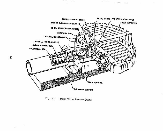
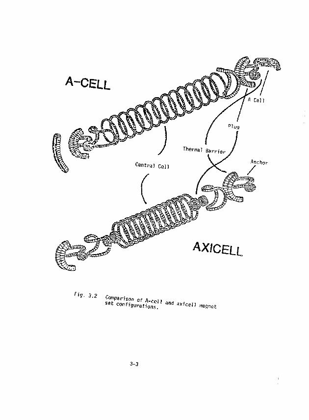
The primary motivation for the modification of the previous MFTF-B A-cell Geometry^ ' ' (FY 1981) to the present axial configuration is its improved engineering promise as a fusion reactor. A comparative evaluation' • of several end plug configurations for tandem mirror fusion reactors with thermal barriers led to the selection of the axicell configuration for its highc.- Q-value, lower plug magnet capital cost, and reduced radial transport. In addition, the axicell operating mode is also required to prevent trapped particle instability as it is presently understood theoretically. In com­paring the axicell configuration to the previous A-cell geometry, one sees a number of differences which significantly affect the reactor physics per­formance, the most obvious being the different magnet sets at the end of each reactor (Fig. 2). In the A-cell TMR, ECRH in the A-cell establishes the peak potential barrier to confine the center-cell ions, and the yin-yang plug retains the function of providing MHD stability to the whole configuration. The functions of electrostatic confinement and MHD stability were separated to allow the A-cells and the yin-yang cells to be better optimized to achieve their respective functions.

In the axicell configuration, the axicell is formed by two circular, high-magnetic-field coils at each end of the central cell. The highest magnetic field generated helps to obtain a sufficiently high

3-1

AXICELLPUMP BEAMS Ml.

ANCHOR SLOSHING ION BEAM ( I I

S t OH, OUASIOPTICAL ECHISI

GYROTRON « l l „

AXKCLL ION BEAMS 131,

AXICELL HYBRID COILS (21

ALPHA PUMPING COIL.

SOLCNOIOAL COIL.

^ G H , ECHtll^YIN-YANO ANCHOR COILS

OIRECT CONVERTER

TRANSITION COIL

FOUNOAYION SUPPORT

Tanden Min-or Reactor (MARS)

A-CELL

AXJCEL.L

? ? ' 3 - 2 ComParUon o f A - C e i i * A magnet

3-3

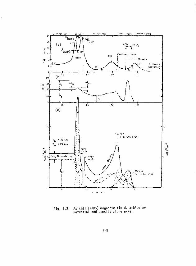
central cell density relative to plug density and results in a suffi­ciently high 0 value. The combination of magnetic constriction and reflection from a potential peak formed by mirror trapped ions in the axicell throttles the flow of ions to the end cells. Those ions con­fined in the central cell by the axicell see only axisyimietric magnetic and electrostatic fields. There is a minimum fraction of central cell ions that must be confined by the end cells to stabilize the trapped particle m o d e w / which is a curvature driven electrostatic instabil­ity sensitive to the fraction of particles passing between regions of good and bad magnetic curvature, becoming severe in configurations having a small fraction of such particles. Regulating this minimum flow of ions from the axicell led to redesigning the ion confining potential iii the yin-yang cells so that more ions reach the end regions. Fig. 3.3a illustrates the magnetic field variation along the axis generated by the axicell magnet configuration of Fig. 3.2. The anchors at the ends of the reactor have the function of providing MHD stability to the whole configuration. Figs. 3.3.b and c show the ambipolar potential and the density profiles at one end of the reactor. These are tailored by the magnetic field, ECRH heating, and neutral beam injection:

• Neutral beams in the axicell generate the first ion confining ootential and fuel the central cell (since the lowest axicell mirror magnetic field is toward the central cell).

• Neutral beams in the transition region are used to pump out particles (by charge exchange and also to fuel the central cell. The ions formed have enough energy to pass over the axicell potential hill into the central cell but not over the potential peak (<j> ) at the ends of the reactor.

• Neutral beam injection off-midplane in the anchor (point a') forms sloshing ions which bounce back and forth in the yin-yang cell, creating density maxima near their turning points. These ions help form the final ion confining potential (<V) and the potential barrier which separates central-cell and yin-yang electrons. The injection of beams on the inside of the yin-yang is preferred to avoid the cooling effect on the ECRH

3-4

CC-n»_rjl c e l l d K l C e ' l t r a n s i t i o n y i n vanrj AnC'-Dr t p i u^

Fig. 3.3 Axicell (MARS) magnetic f i e ld , ambipolar potential and density along axis.

3-5

heated electrons in the potential peak * by the newly formed electrons from the injection.

9 ECRU at the thermal barrier minimum (point b) serves to reduce the fraction of cold central cell electrons passing into the anchor and confine them magnetically. A reduction of the cold-electron density required for quasineutrality further deepens the thermal barrier potential minimum.

• ECRU heats electrons trapped within the outer peak in ion density in the anchor. This heating increases dramatically the height of the corresponding potential peak forming the final ion confining potential.

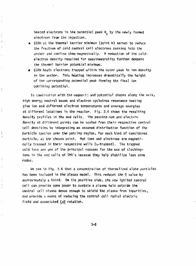
In combination with the magnetic and potential shapes along the axis, high energy neutral beams and electron cyclotron resonance heating give ion and different electron temperatures and average energies at different locations in the reactor. Fig. 3.4 shows the resulting density profiles in the end cells. The passing-ion and electron density at different points can be scaled from their respective central cell densities by integrating an assumed distribution function of the particle species over the pasiing region, for each kind of considered particle, at the chosen point. Hot ions and electrons are magneti­cally trapped in their respective wells (u-trapped). The trapped cold ions are one of the principal reasons for the use of sloshing-ions in the end cells of THR's because they help stabilize loss cone modes.

Vie see in Fig. 3.4 that a concentration of thermaiized alpha particles has been included in the plasma model. This reduces the Q value by approximately a third. On the positive side, the now ignited central cell can provide some power to sustain a plasma halo outside the central cell plasma dense enough to shield the plasma from impurities, and provide a means of reducing the central cell radial electric field and associated E_xB_ rotation.

3-6

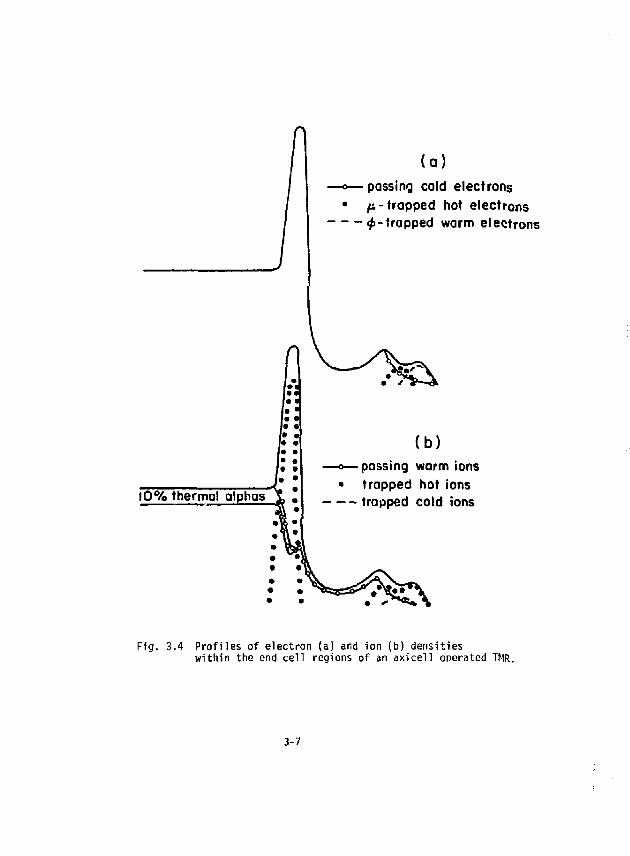
(a ) passing cold electrons

• fi-trapped hot electrons — ^-trapped warm electrons

10% thermal alphas

passing worm ions trapped hot ions trapped cold ions

Fig. 3.4 Profiles of electron (a) and ion (b) densities within the end cell regions of an axicell operated TMR.

3-7

3=2 THE PLASMA MODELING CODE

3.2.1 General Description of the Plasma Model

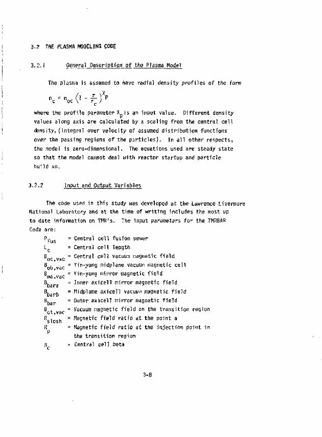
The plasma is assumed to have radial density profiles of the form

"c"%cO-f) P

where the profile parameter X is an input value. Different density values along axis are calculated by a scaling from the central cell density, (integral over velocity of assumed distribution functions over the passing regions of the particles). In all other respects, the model is zero-dimensional. The equations used are steady state so that the model cannot deal with reactor startup and particle build up.

3.2.2 Input and Output Variables

The code used in this study was developed at the Lawrence Livermore National Laboratory and at the time of writing includes the most up to date information on TMR's. The input parameters for the TMRBflfi Code are:

P p u s = Central cell fusion power L = Central cell length B r ., = Central cell vacuum magnetic field B , = Yfn-yang midplane vacuum magnetic cell B = Yin-yang mirror magnetic field B, = Inner axicell mirror magnetic field B. . = Midplane axicell vacuum magnetic field B b = Outer axicell mirror magnetic field B . „,„ = Vacuum magnetic field on the transition region OL»vac R 1 , = Magnetic field ratio at the point a R = Magnetic field ratio at the injection point in

the transition region g = Central cell beta

3-8

6 = Axicell beta P Bjj = Ym-yanp beta C Q = AlDha particle fraction confined in the central cell X = Plasma density profile exponent

LA-cell = Y i n">' a n5 c e 1 1 length Lj = Transition region length G = Ratio of total ior. density to passing ion density

at the point b FIom'z = C h a r 9 e exchange ionization parameter in the transition

region (the neutral product after a charge exchange reaction can be ionized, and has to be pumped out again).

Pcx = Charge exchange coefficient in the transition region

The output parameters consist of • All the particle energy exchange rates f The particle loss rates from the different reqions of the reactor • The temperature/average energy of the different particle kinds • The different densities and potentials in the central cell,

the axicell (pb and pc), the pump beam injection point (i), the transition region (t), the sloshing ion injection point (a'}, the thermal barrier potential minimum (b), the inner mirror of the anchor (mp), and at the potential maximum in the anchor (a).

• Injection powers and ECRH powers required • The plasma radius, the first wall neutron loading and the reactor

0 value.

3-9

3.2.3 General Jescription of the TMRBAR Coti"

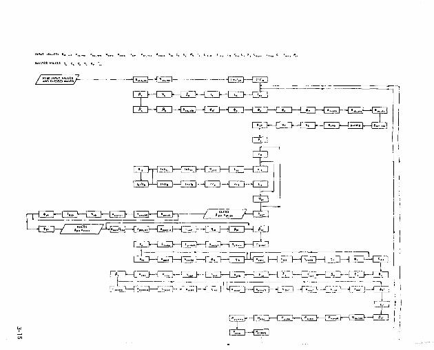
A complete 1is;ing of all the equations used in the TMRBAR code is given in Appendix 1. The program contains eleven iterative loops (see Fig. 3.5). Starting from the inner ones, we have

• Three nested loops to calculate all the axicell parameters. (8) The equations used form the Logan-Rensink plug modeV .

• Six simple loops to calculate the density of the different particle kinds and the ambtpolar potential (using quasineutrality) at the points pb, i, b, t, mp, and a', respectively.

• One loop to compute the electron temperature in the central cell (T ) and the electron potential to temperature ratio (n e). This loop uses the quasi neutrality equation and the electron energy balance. A Newton's method' ' (with two unknowns) helps to solve for T and n e-

• Finally, the outermost loop uses the ion energy balance to compute 7)c = 4>C/TC.

After reading the input parameter, the program calculates (the equations listed below are in the Appendix):

• The plasma magnetic field in the axicell (Eq. 1) • The vacuum magnetic field at the injection point (Eq. 2) • The fusion reaction parameter (Eq. 3) 9 The alpha particle confining parameter (Ea. 4)

After entering the ion energy loop and the central cell quasineutrality and electron energy loop, the program calculates

• The slowing down alpha particle energy fraction on electrons (Eq. 5) • The central cell density (Eq. 7) • The central cell plasma radius (Eq. 9) • The first-wall loading (Eq, 10) • The central cell plasma volume (Eq. 11) • The profile averaged betas in the central cell, axicell, and

anchor, respectively {Eq. 12, 13, 14) • The plasma magnetic field in the axicell (Eq. 15) • The potentials 4>a,, <f>b, <(>c, * e, <)>t (Eq. 16)

3-10

• The effective anchor injection energy (Eq. 17) • The plasma magnetic fields at the points b, a, and a',

respectively (Eqs. 18, 19, 20) t The mirror ratio at the sloshing ion injection point (Eq. 21) • The effective mirror ratio of the sloshing ions (Eq. 22) • The barrier and the transition reqion volumes (Eqs. 23, 24) • The axicell inner mirror ratio (Eq. 25) • All the axicell parameters (Eq. 36-40). These equations are a

self consistent set which form the Logan-Rensink plug model. A maxwellian formula is used to calculate the potential difference A (Eq. 40). pc

• The axicell neutral beam current (Eq. 41) • The plasma axicell outer mirror ratio (Eq. 42)

The next step in the program is to guess the values of the potential * L, and the passing ion density at the pm'nt pb. These guesses will be used tc calculate the passing ion density, the passing alpha-particle density, the potential-to-electron-temperature ratio n ., the alpha particle fraction and the potential A . (Eq. 43, 44, 45). A few iterations are needed for the code to converge toward the solution of the potential <J> . .

The program uses a quasineutrality condition at the point pb. The different densities which are used to help calculate the potential ^pb a r e f o L , r , c l through a mapping from the central cell where magnetic field, ambipolar potential and density are known. '

The code then calculates the plasma magnetic field at the pumping injection point (Eq. 46) and follows the same procedure, which is used to calculate the potential Q ., to compute the potential $ . (Fq. 48, 49). The mirror-ratio calculations of Rj, o 1 d and R t o l d are intermediate steps to evaluate the different densities at the point i.

3-11

After exiting the A . loop, the code computes: t The beta value at the injection point (Eq. 50) • T h e m i r r o r r a t i o s Rplrnir a n d RpRmir (Ec>- 5 1 ' • The pumping energy at the point i (Eq. 54).

The same procedure followed to calculate the potentials a . and <j>i ii carried out to evaluate the barrier and the transition region potentials (<j>b, <p.) (EQ. 56. and Eq. 58),

The program then calculate • The alpha particle fraction and the beta in the transition

region {Eq. 60 ; t The electron cutoff energy E^ (Eq.61 ) • The parallel pressure in the barrier region {Eq. 62 ) • The rest of the pressure in the barrier region (Eq.63 ) t The hot electron average energy in the barrier (Eq.64 ) • The passing cold electron fraction {Eq.65 ) t The hot elecf.'an density in the barrier (Eq.66 )

t ine cold electron density in the barrier (Eq. 67) • The hot electron density at the point a (Eq, 68) • The sloshing ion density at point a (Eq. 69) t The warm electron density at a (Eq. 70) • The profile-averaged beta at a (Eq. 71)

Quasineutrality conditions are again used to find the potential at the sloshing ion injection point a' and at the inner maximum f =1d of the anchor (point mp). Other parameters calculated in the a' loop are the sloping ion density and the hot electron density at the point a' (Eos. 73, 74).

3-12

The effective beta value and the vacuum magnetic field at the point a' are computed, followed by

t The barrier pumping power (Eq. 77) • The transition pumping power (Eo. 78) • The total pumping power (Eo. 7*3) • The neutral beam power at the point a' (Eq. 80) • The ECRH power at a (Eq. 81) • The Syncrotron power (Eo. 82) • The ECRH power at b (Eq. 83)

As mentioned above, the quasineutrality condition and the electron energy equation in the central cell close the first big loop. The quasineutrality condition includes (Eq. 101), respectively

t The loss of ions by burn through fusion reactions (Eq. 99) • The loss of ions and electrons through the ends (Eq. K l ) t The addition of electrons from sloshing ion beams (Eq. 85)

The electron energy balance includes: • Cooling from the axicell injection beam electrons (Eq. 101) • ECRH heating at a and at b (Eos. 103, 104) i Drag from ions in the central cell (Eii. 105} • Cooling from the sloshing ion-beam electrons (Eq. 106) • Pastukhov loss of electrons (Eq. 107) « Addition of energy from alpha particle (Eq. 108) • Loss of electrons through charge exchange pumping (Eq. 109)

The ion energy balance written in a newton's form (newton's method) concludes the calculations in the most outer loop. The ion energy balance includes:

• Pastukhov energy losses (Eqs. Ill , 112) • Addition of eneray from alpha particles (Eq. 113) • Addition of ions from the axicell beams (Eq. 114) • Addition of ions from the pumping beams (Eqs. 115, 116).

3-13

Before ending, the program calculates t The total ion fueling rate/loss rate from the whole reactor

(Eq. 119) • The reactor Q value (Eq. 120) • The beaM trapping fractions for the sloshing ions and for

the axicell (Eqs. 124, 126).

The Code ends by checking the adiabaticity condition (Eq. 127) and by reading the output values.

3.3 COMPUTED TANDEM MIRROR PARAMETERS

Table 3.1 shows the reactor parameters for coupling to a synfuel plant 2 which uses a fusion power of 3500 Mwf, a first wall loading of 5 MW/m

and a first wall radius of 0.6 m. Thsse numbers represent state of the art TMR fusion parameters in considering reactor Q value, magnet cost, radial transport, and trapped particle instability; but are not appro­priate for coupling to the blr.nket used in other sections of this

p report, where P p = 2600 Mwf, r w = 2 MR/m and r w = 1.5 m are taken. These later numbers will be sealed in future work to match the MARS TMR parameters. Figure 3.6 shows the power balance of a MARS electri­city producing plant^ ' which uses the TMR parameters of Table 3.1. The overall efficiency of the system is 0.34 or 0.39, depending on the blanket multiplication factor (1.37 or 1.16).

3-14

CuuMO v»VVlS \- ^ , v, i^ 1), t # i

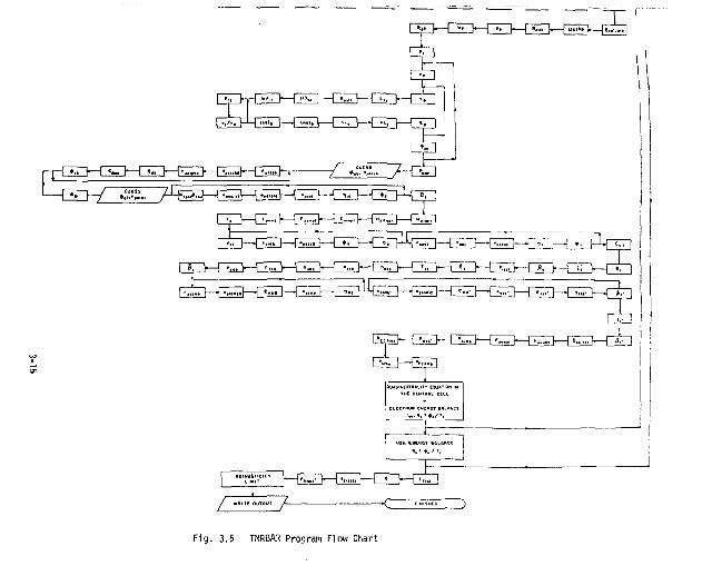
F1g. 3.5 TMRBAR Proqram Flow Chart

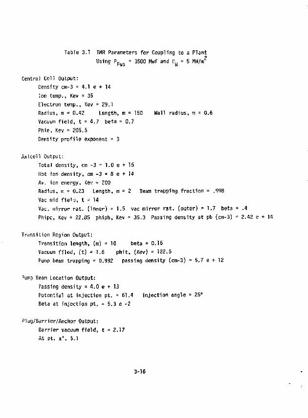
Table 3.1 TMR Parameters for Coupling to a Plant Using P p u s = 3500 Mwf and r H = 5 MW/m 2

Central Cell Output: Density cm-3 =4.1 e + 14 Ion temp., Kev = 35 Electron temp., Kev =29.1 Radius, m = 0.42 Length, m = 150 Wall radius, m = 0.6 Vacuum field, t = 4.7 beta = 0.7 Phie, Kev = 205.5 Density profile exponent = 3

Axicell Output: Total density, cm -3 = 1.0 e + 15 Hot ion density, cm -3 = 8 e + 14 Av. ion energy, Kev = 200 Radius, m = 0.23 Length, m = 2 Beam trapping fraction = .998 Vac mid fieij, t = 14 Vac. mirror rat. (inner) = 1.5 vac mirror rat. (outer) = 1,7 beta = .4 Phipc, Kev = 22.85 phipb, Kev = 35.3 Passing density at pb (cm-3) = 2.42 e + 14

Transition Region Output: Transition length, (m) = 10 beta = 0.16 Vacuum filed, (t) = 1.6 phit, (Kev) = 122.5 Pump beam trapping = 0.992 passing density (cm-3) = 5.7 e + 12

Pump Beam Location Output: Passing density = 4.0 e + 13 Potential at injection pt. = 61.4 injection angle = 25° Beta at injection pt. = 5.3 e -2

Plug/Barrier/Anchor Output: Barrier vacuum field, t = 2.17 At pt. a', 5.1

3-16

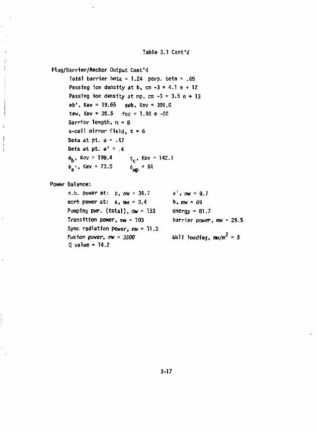
Table 3.1 Cont'd

Plug/Barrier/Anchor Output Cont'd Total barrier beta = 1.24 perp. beta * .65 Passing 1on density at b, cm -3 = 4.1 e + 12 Passing ion density at mp, cm -3 = 3.5 e + 13 eb", Kev = 19.65 eeh, Kev = 391.S tew, Kev = 35.5 fee = 1.98 e -02 Barrier length, m = 8 a-cell mirror f i e l d , t = 6 Beta at pt. a = .47 Beta at pt. a' = .4 <|>b, Kev = 198.4 $ c , Kev = 142.1 <|>a>, Kev = 73.S A - 64

Power Balance: n.b. power at: p, mw = 34-7 ecrh power at: a, mw = 3.4 Pumping pwr. (total), row = 133 Transition power, mw = 103 Sync radiation power, mw = 11.3 Fusion power, m = 3500 Q value = 14.2

a', mw = 8.7 b, mw = 69 energy = 81.7 barrier power, mw = 29.5

o Wa7j 7oadfng, m/m = S

3-17

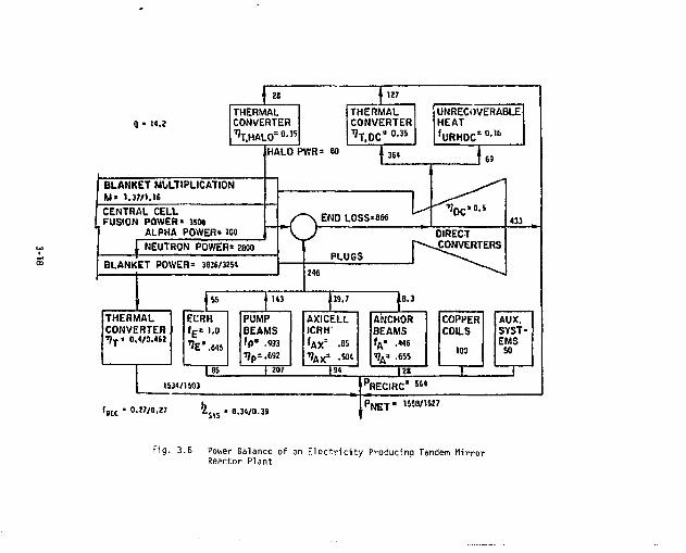
f p [ c • 0.27/0.27 £ S Y S • 0.34/0.39

F ig . 3.6 Power Balance o f an E l e c t r i c i t y Producina Tandem Mi r ro r Resctor Plant

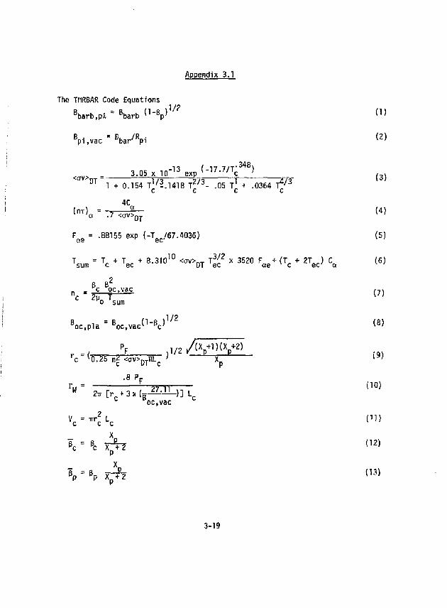
Appendix 3.1

The TMRBAR Code Equations W P * - <Wb " V ^ o> Bpi,vac = B bar / R p i ( 2 )

<av> 3 .05x 1 0 - 1 3 exp<-^^ T c 3 4 8 ) , 3 ) a v DT T71 27? 1 275" **' 1 1 + 0.154 TV*.1418 vj • .05 r + .0364 1Z c c c c

4C

F Q a = -BS155 exp {-Te c/67.4036) (5)

Tsun, " T c + Tec + 8 - 3 ' ° 1 0 < 0 V > DT T e f * 3 5 2 ° F a e + <Tc + 2 V C« ™

_ _ c oc, vac in*. n c " 2p T ( 7 )

o sum Boc,Pla = V * ^ V * < 8 >

(10)

(12)

(13)

/ PF ,i/ 2/^V 1 ) {V } XP

*) 'c l0.25 n£ <cv>DTnLc

,i/ 2/^V 1 ) {V } XP

r w = .8 P F r w =

277 [r c + 3 oc.vac

V " ? L c

V pc V

X p + 2

V BP XP

X +2

3-19

Bop,pla = Bop,vac » V " (15)

V = n a < T e C W e e ' V c V W e e ' *T = , V e c ( 1 6 )

E in jab = ETnja> + * b " V 0 ' )

Bob,PU * B ob l W c ( 1 V * < 1 8 >

V p l a = * l « * * a o b . » a c " V / 2 <">

B oa . , P l a l + ( V - * a . - V E i n j a .

s l o s h

P

= B o a " W B o b , p l a ( Z 1 )

B „ = ma, vac e f f S " s l o s h B o b , v a c ^ - p K ) 1 / 2 n + ( ^ U / E , - r i s a ] (ZZ)

b c Aceil B o b j V a c \^_^ )

if 2(}i

P I + n c ( . 9 E p - T c ) e X p ( l - ^ ) + ( . 9 E p - T c - T e c ) n c C a e x p ( - - ^ ) (27) n„ s

• 9 E P + T e c

3-20

n ih = np ' nc e x p l-f*) - C

a

n c e x p f " - T 2 ^ ( 2 8 )

Ecp = yiRpg-D (29)

Vff = V / ( T + V E inJP ) ( 3 0 )

an U e . ) = in (5.7xlO 1 3 T £ C/nJ / 2) (31)

An ( A . ) = * n ( l . 4 x l 0 1 5 ^ p ) (32) P '

E = U. . +E — ] / ( l + — \ (33) Lp \ i n j p cp t D } f \ T D ; <• '

E-!„4„ 3/Z

^ = . „ _ e c 1 ( 3 4 )

E L P

^ s = 3 - 9 x 1 ° 1 2 E i n j p

3 / 2 l B 1 0 R

P e f f f c n X i i - ( 3 5 )

2 x l 0 1 3 T 3 / 2 / E , . \

(iw)p " (nT) s(nT)D/[(n T) s+(rT)D] (37)

? i n 1 3 T 3 / 2

d r a g *n A e i

E p = ( E i n j p - E L p ) ^ y f i + 1 - 5 T

e C <39)

V = Tec * n l ^ i r ) ( 4 0>

3-21

PNBp = e ^p ^ b Einjp Tnifl (41)

'bar ° W'V* ec

V - V " in X1i1gpb "paspb + 2 "paspba "paspbe «P H p * >

r = paspb _ T

a P b " Vspb ' Pb " Pb e c

B , • = B • J 1 -B . p la .p i vac,pi pi

B R,

bar B . K bar

bold _ ~ n . ,1 /2 ' " to ld • , , , 1/2

'pi pc

*pi = n p i T ec

1.16 X . . „ ., . + 2,-

V P i «P ^ V * * ec

2 , J o * ^ ^ ^ i f l V s p l t V T e c ^ ( 2 T

e c ! V % a i p i a Pi

R. 'plffljr B

paspi B 2 . pi,vac

- bar D _ barb R p i

p2mir B Pi

"pumpl rjL

^ p l m i r s i " 2 G i n j p i

V -*pb pump2 " , _ . 2 „

1 H p l m i r S 1 " y i n j p i

(42)

(44)

(45)

(46)

(47)

(49)

(50)

(51)

(52)

(53)

3-22

Epump " M a x ( E pumpT Epump2^ (54)

(55)

T pc ec

n+ = TI + an

( 1 . e x p e ) ( ec pasb ec ec

ec

I u 0 1 JHSbSL, + e x p ( ^ _ , (56)

ec J

* Pc L X ^ g n p a s t + 2 n p a s t a .

h = n t T ec

pas tot a t n past

fl _ % huu "past t y T e c ) H 2 T e c + T c ) n D a s t a

1 B 2

ot,vac F , . *b

b " V1"

V = 2 y o "pasb | -5 T c + W + ( 1 - F e c } G x ' 2 E b

^~1 B ob.vac

(G" X£i£c 1^t 1-iTW ) E in.ia'^b-^-] + M B 2 (

ob,vac J

2u„ n„ X.*.«T + GF T +E. . . { ^ rest o pasb JlUg c ec ec in ja ' *sloshp

2 F - ob.vac ^bp" rest

)

1 ec \3/2

1 + ec

(57)

(58)

(59)

(60)

(61)

(62)

(63)

(64)

(65)

3-23

n e h b = { 1 - F e c ) G n p a s b

"ecb = G Fecnpasb

=

nehV ma.vac " oa.pjta) e h a " / T + A * V 1 ' 7

f f i B , 1 i0ma,vac ob,p£av

.2E. •.-•«• ww ( '^fesr newa = nisa" neha

B a = ( " e w a T e W

+ - V e h a 1 ^ 2 * E1nJ»w1sa) 2»o sMa_

< B o b , v a c x s 1 o s h >

V V * 4 " 1 e x p

" isa J " ( G - X J t i V n p a s b

ffynpA "ectnp ^ T e c ' lXAUgnpasmp +

/V*ap.\

£g"pasmp ' "pasmpa'

1 /2 / „ \ 1.24 ' oa' ,pita i

B. ob,p£a

(66)

(67)

(68)

(69)

(70)

(7)}

(72)

(73)

"eha' "ehb * ma.vac~ oa'.pia)

• 2L f B - B ) * ma,vac op,paa' [

a 2 Vpasa' T

C

n isa* W W e e * ^ J ^ ^ ) "eha"

e • l

f a '

TZ "oa'.pAa

n °oa',vac

ob,paa

p oa'.pla 1 -B a ,

(74)

(75)

(76)

3-24

W = 4.49X10" 3 3 n ^ V b x | ( H . 0 4 4 1 R b o l d ) 3 - 3 3 ( 1 + 4 C a b + 1 6 C ^ ) E p u m p

/ ll15Xai*fl\ Fiomzhu9 , 7 7 )

l l . l6X„,- 0 r l-V ITT n 2 . 3 3 n T 1.5 K ' n

\ * U g / ( X i U g _ 1 ) PcxTc

W • 4 - 4 9 x l ° 3 3 v t " p a s t ( 1 + 0 . 0 4 4 1 R t o 1 d ) ( l + 4 C a t + 1 6 c 2 t ) X

p / K 1 6 X a i £ q I F

X&ifcg , „ ,

rNBa' 1 0 , / ? 0 «»in R--ffc ( 1 . 5 8 x l 0 l u E ^ t ) R " , r ~ " 10 effs inja B o b j p i a

10.66 x l O - ^ V ^ f f ^ - T , . )

"sync = Xksync Bob,vac "pasb Vb ( V ^ T ) < 8 2'

[ 2 - n / .68 \ Xkmub T"Fec npasbEh*TVb feal^p^R^/

( f ) 2 ] (83) + P sync

P 1 - pump p u m | > / v ' Epump ! 8 4 >

inja"

I- - P^ (86) X E1njp

3-25

15. An * . . = An {2 1 0 ' V T T / n ) n 4 ec c c '

T_ *" Aee = *" ^ ' ^ 6 " "

n ec \

VT > ec T

An X. = An { 9 . 3 4 x l 0 1 3 - 7 7 2 6 1 %

a(R) = ( l + i ) 1 / 2 An

tf(f) = 0 + f ) 1 / 2 An

( l+i) 1 / 2+V

( i+ i ) i / 2 + f 1 1 )^TT

(/IT) 3. I x l O 1 1 cr{§)

cct

(n t )

[An x ^ ( l + 4 C a ) T y 2 ] * exp J 1

4C

acreated .7<ov> DT

(87)

(88)

(89)

(90)

(91)

(92)

(93)

(n t )

(nx)

(n t )

(nx)

c i = ^ n T > c a + t n T } c r e a t e d

3.6 xlCT a(R) ea

( t o Xee T e c 2 ) *e ^ i f

( l + 2C a )4C a

er .7<av> DT

1 ce 1 1

(94)

(95)

(96)

(97)

3-26

'ei

T 1.5 t^\ - i n 1 3 - ec

1 2 en„ < cxv > „ V X

'pburn ~ I e n c DT T c{X p +l j (X p +2)

(98)

(99)

T = en V 1 <l*2C«>i

(nxl . " (nx), 'ci (X +1)(X +2) ce J 1 p '' p (100)

F n = T . + T ,. + I , pB pburn ptran a'

ex ~ * injp " loss " *pc' pc' x

TECRHa B PECRHa

TECRHb = PECRHb

TEei ( nx ) e i (X p+U(X p+2)

TEslosh = ( V " *pc} V

*"? (*„ +Tj M1+2CJ2

T - o e c' u p* or 'Eetran " ( n t ) c e

v c (X p+l)(X p+2)

TEfus = e n c < o v > D T Ea Fae Vc (X p*l?(X p+2)

Epump ~ pump ' cx'**pi~*pc

(101)

(102)

(103)

(104)

(105)

(106)

(107)

(108)

(109)

3-27

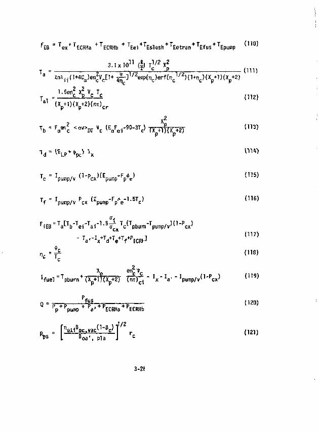
FEB = T ex + T ECRHa +TECRHfa + T E e i 4 TEslosh + T E e t r a n + T Efus + TEpump t l l Q )

T = z V-T/2 J 1/2 ~ • ( 1 1 1 )

a tnA^d^Jen^n+gf-r^eap^Jerfdj^'^d+ncXX+lXX +2) c

l.Senj: xj; V„ T j = C p C C ( 1 1 2 j

t X p + 0 ( x p + z ) { n T ) c r

X 2

Tb = F B « | « *>DT VC < E a F a , - 9 0 - 3 V < X p * 1 ? ( y 2 ) { 1 1 3 )

Tf" W v ^ ( W F p V 1 > 5 V 0 1 6 )

ffi FiE8 = T a [ T b " T e r T a i " 1 , 5 b ^ x

T c l T p b u n ) " T p u n i p / v ) , 1 " P c x )

T a < - W V T f + P I C R ^

X. er?V„

P fus Pp + Ppu!tip + P a ' + PECRHa + PECRHb

%S

(117)

(118)

!fue1 =Tpburn+(X+l)(x+2) XmH " V V " ^ump/v 0 "^ ( 1 1 9 )

P P c l

(120)

NM^f r (121) L B o a ' , pla J c

3-26

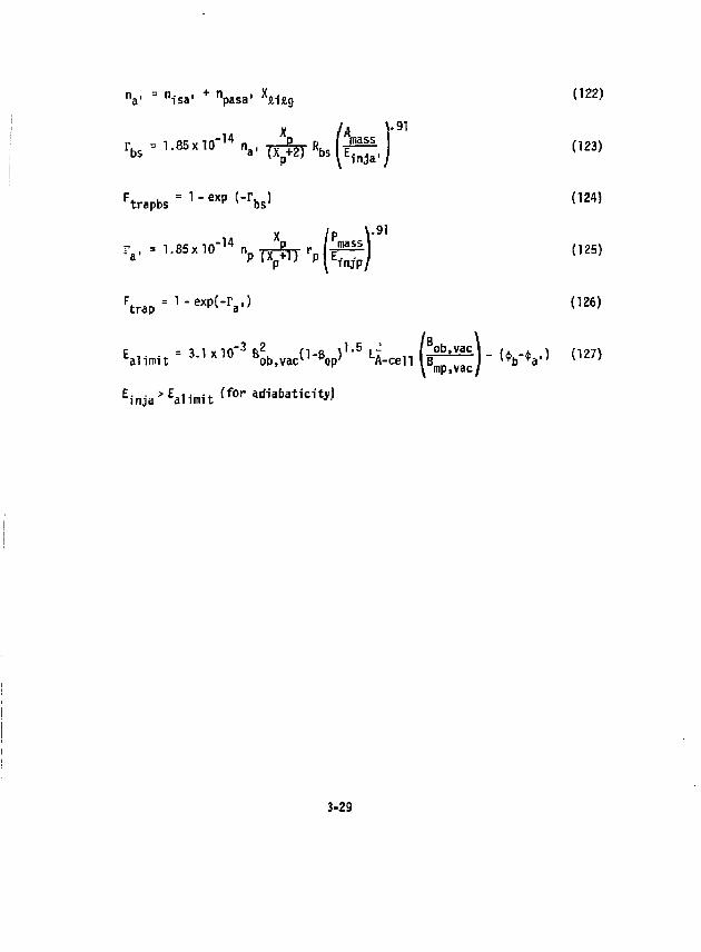
V = "isa' + npasa' hu5

( 1 2 2 )

r t e - l .« ixlO- 1 4 n, l T 3 i^ r I l t e ^ i J (123)

Ftrapbs = 1 - e x ^ - r b s 5 < 1 2 4>

F t r a p = 1-exp{-r a,) 026)

E a1 i . i t = 3 J x 1 0 " 3 ^ b . v a c ^ V 1 ' 5 L i c e l l ( ^ ) " < V V > < 1 2 / )

E i n j a > E aHmi t f o r arffatatfcity]

3-29

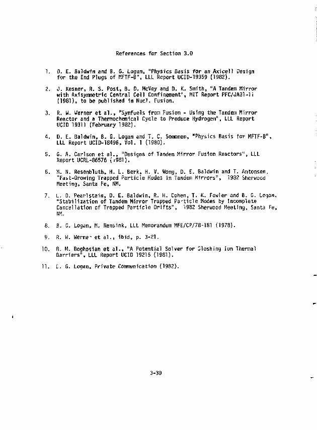
References for Section 3.0

1. D. £. Baldwin and B. S. Logan, "Physics Basis for an Axicell Design for the End Plugs Of MFTF-B", LLL Report UCID-19359 (1982).

2. J. Kesner, R. S. Post, B. D. McVey and D. K. Smith, "A Tandem Mirror with Axisymmetric Central Cell Confinement", MIT Report PFC/JA31-1i (1981), to be published in Nucl. Fusion.

3. R. W. Werner et al., "Synfuels from Fusion - Using the Tandem Mirror Reactor and a Thermochemical Cycle to Produce Hydrogen", LLL Report UCID 19311 (February 1982).

4. D. E. Baldwin, B. G. Logan and T. C. Somonen, "Physics Basis tor MFTF-B", LLL Report UCID-18496, Vol. 1 (1980).

5. G. A. Carlson et al., "Designs of Tandem Mirror Fusion Reactors", LLL Report UCRL-86576 (i981).

6. tl N. Resenbluth, H. L. Berk, H, V. Wong z D. £. Baldwin and T. Antonsen, "Fast-Growing Trapped Particle Modes in Tandem Mirrors", 1982 Sherwood Meeting, Santa Fe, NM.

7. L. D. Pearlstein, D. E. Baldwin, R. H. Cohen, T. K. Fowler and B. G. Logan, "Stabilization of Tandem Mirror Trapped Particle Modes by Incomplete Cancellation cf Trapped Particle Drifts", 1982 Sherwood Meeting, Santa Fe, NM.

8. B. G. Logan, M. Rensink, LLL Memorandum MFE/CP/78-181 (1978). 9. R. W. Werne- et al., ibid, p. 3-21.

10. B. M. Boghosian et al., "A Potential Solver for Sloshing Ion Thermal Barriers", LLL Report UCID 19215 (1981).

11. I. G. Logan, Private Communication (1982).

3-30

SECTION 4 ENERGY BALANCE - THE TANDEM MIRROR REACTOR

AS AN ENERGY SOURCE Contributors:

F. L. Ribe, R. W. Werner, T. H. Zerguini

TABLE OF CONTENTS Section 4.1 TANOEH MIRROR PARAMETERS 4.2 THE INFLUENCE OF Q ON THE REACTOR ENERGY BALANCE

AND ON THE SYNFUEL PLANT

LIST OF TABLES T^b,e 4.1 Physics parameters for a TMR producing 3500 Mwe at

a q = 14.2

LIST OF FIGURES Figure 4.3 Power balance of a TMR used for producing Synfuels,

Q = 25 and M = 1.37 or 1.2 (Synfuel model) . . . . 4.2 Power balance of a TMR used for producing Synfuels,

Q = 14.2 and M = 1.37 or 1.2 (current MARS model)

I

4.1 TANDEM MIRROR PARAMETERS

Table 4.1 shows the physics parameters for a reactor producing 3500 Mw of fusion power at a Q value of 14.2 as computed with the TMRBAR C O d e described in Section 3. These values are not appropriate for coupling the reactor plasma physics to the engineered blanket found in other sections of this report and to the synfuel plant itself.

Late in the synfuel study year the parallel MARS study, whose physics parameters we follow for synfuel use, indicated this lesser value of Q than the value of 25 we have cited in other portions of this study. At the writing of this report the WARS Q was (4.1. Die impact of tni's smarter Q l's felt both in the reactor pt orroance and its energy balance but ft also impacts the synfuel plant and its requirement for energy in both electrical and thermal form.

4.2 THE INFLUENCE OF Q ON THE REACTOR ENERGY BALANCE ANO ON THE SYNFUEL PLANT

Figure 4.1 illustrates the energy balance for a Q of 25 and a reactor injection/heating iystem used for the synfuel work.

Figure 4.2 illustrates the energy balance for the more recent Q value of 14.2 plus the use of a more sophisticated injection/plasma heating system .aad a sos>r& detailed energy recovery system fcr the direct CDnveri&r.

Comparing these two figures in terms of energy delivered to the synfuel plant by a 3500 Mwf reactor it can be seen that both the thermal differences and the electrical dif dr ices are significant. The reason is m^niy due to the fact that at the 14.2 Q value the reactor is very nearly at I). -akeven as far as utilization of the direct convertor output is concerned. Both the high voltage dc electrical energy and the direct convertor thermal energy, after its conversion to electricity, have to be fed back to the reactor to drive it. When Q is as high as 25, not only can the thermal energy f r o m the

4-1

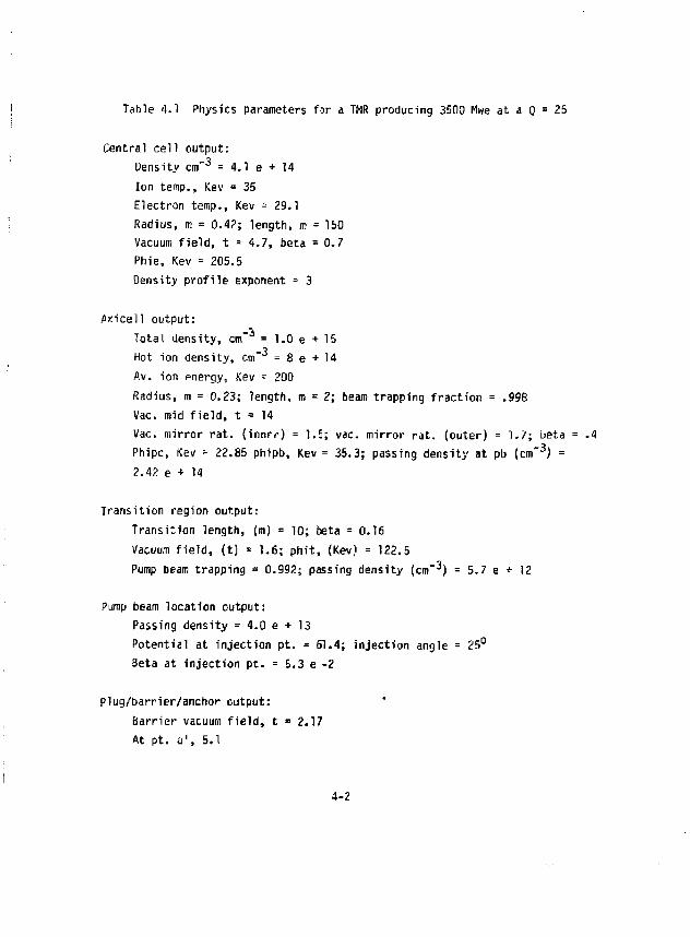
Table 4.1 Physics parameters for a TMR producing 3500 Mwe at a Q = 25

Central cell output: Density cm = 4.1 e + 14 Ion temp., Kev = 35 Electron temp., Kev = 29.1 Radius, m = 0.42; length, m = 150 Vacuum field, t = 4.7, beta = 0.7 Phie, Kev = 205.5 Density profile exponent = 3

Axicell output: Total density, cm" = 1.0 e + 15 Hot ion density, cm = 8 e + 14 Av. ion energy. Kev = 200 Radius, m = 0.23; length, m = 2; beam trapping fraction = .998 Vac. mid field, t = 14 Vac. mirror rat. (innrr) = 1.5; vac. mirror rat. (outer) =1.7; beta Phipc, Kev = 22.85 phipb, Kev = 35.3; passing density at pb (cm" 3) = 2.42 e + 14

Transition region output: Transition length, (m) = 10; beta = 0.16 Vacuum field, (t) = 1.6; phit, (Kev) = 122,5 Pump beam trapping = 0.992; passing density (cm - 3) = 5.7 e + 12

Pump beam location output: Passing density = 4.0 e + 13 Potential at injection pt. = 61.4; injection angle = 25° Beta at injection pt. = 5.3 e -2

plug/barrier/anchor output: Barrier vacuum field, t = 2.17 At pt. a', 5.1

4-2

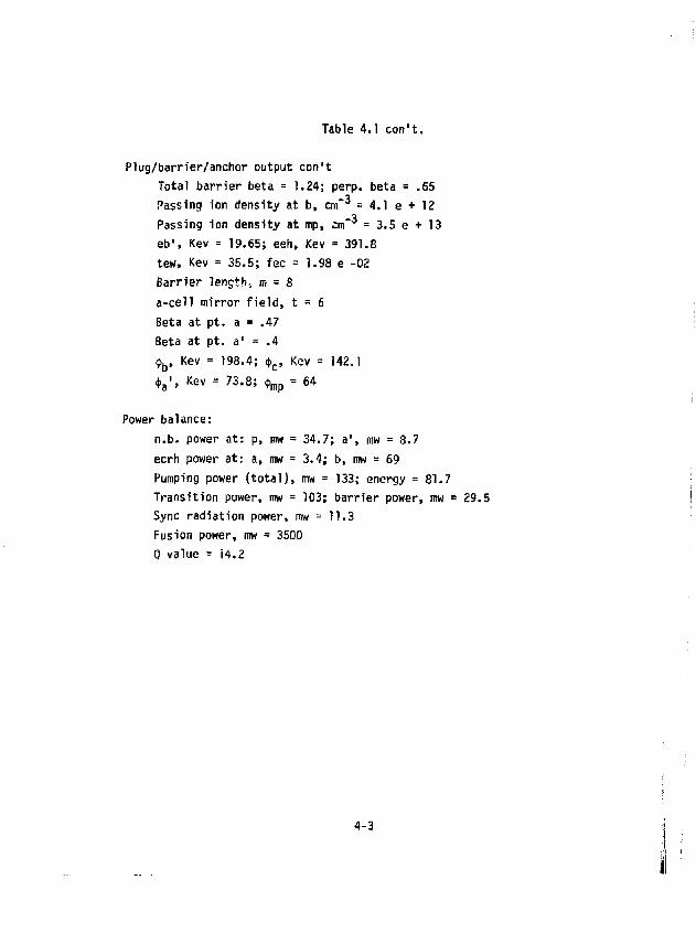
Table 4.1 con't.

Plug/barrier/anchor output con't Total barrier beta = 1.24; perp. beta = .65 Passing ion density at b, cm = 4.1 e + 12 Passing ion density at mp, cm = 3.5 e + 13 eb', Kev = 19.65; eeh, Kev = 391.8 tew, Kev = 35.5; fee = 1.98 e -02 Barrier length; m = 8 a-cell mirror field, t = 6 Beta at pt. a = .47 Beta at pt. a 1 = .4 <t>b, Kev = 1 9 8 . 4 ; <t>c, Kev = 142.1

$ a ' , Kev = 7 3 . 8 ; $ m p = 64

Power balance: n.b. power at: p, mw = 34.7; a", mw = 8.7 ecrh power at: a, mw = 3.4; b, mw = 69 Pumping power (total), mw = 133; energy =81.7 Transition power, mw = 103; barrier power, mw = 29.5 Sync radiation power, mw = 11.3 Fusion power, mw = 3500 Q value = i4.2

4-3

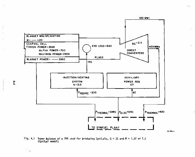
420 MWI

BLANKET MULTIPLICATION M = 1.20 CENTRAL CELL FUSION POWER = 3500

ALPHA POWER=700 NEUTRON POWER=2800

BLANKET POWER = -3360

o END LOSS = 8 4 0

PLUGS

INJECTI0N/HEATIN6 SYSTEM 1> = 0.6

RECIRC

n

= 0.5

OIRECT CONVERTERS

AUXILIARY POWER REQ

67

P T H E R M A L = 3 3 6 °

67

P E L E C = 2 4 0

420 MWe

tn 1 TO SYNFUEL PLANT _ _ _ ___ \

Fig. 4.1 Power balance of a THR used for producing Synfuels, Q • 25 and H = 1.37 or 1.1: (Synfuel model)

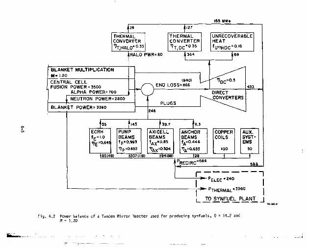
, 28

THERMAL CONVERTER

0.35 'T,HALO ;

HALO PWR=80

BLANKET MULTIPLICATION M = 1.20 CENTRAL CELL FUSION POWER = 3500

ALPHA POWERS TOO

i I 2 f

T H E R M A L

CONVERTER ^ T . D C " 0 3 5

155 MWt

UNRECOVERABLE HEAT f U R H D C ° 0 1 6

NEUTRON P0WER=2800

BLANKET P0WER=3360

55 f l43

ECRH f E . . . 0 7; E=0.S4!

•85148)

PUMP BEAMS fp=0.993 -r\ p =0.692

139.7 AXICELL BEAMS f A X - - 0 . 8 5

^ A x = 0 . 5 0 4

•2071118) (94188)

8.3

ANCHOR BEAMS f A =0.446

1JA=0.655

' P R E C I R C = 5 6 4

)28

COPPER COILS

100

AUX. SYST­EMS

50

586

r: ~ r E L E C * " u

* - p T H E R M A L ' 3 3 6 0 I U _I? SYNFUEL PLANT J

Fig. 4.2 Power balance of a Tandem Mirror Reactor used for producing synfuels, Q • 14.2 and M = 1,20

direct convertor go directly to the thermochemical plant but there is also an excess of high voltage dc that can also be utilized Since the synfue! plant has significant internal electric demands this extra convertor elec­trical is quite significant. This is true in either our Joule-Boosted or our Fluidized Bed design case. Clearly high Q values are desirable. This applies also to the case where the reactor is used for the production of electricity as well as synfuels.

4-6

SECTION 5 THE LITHIUM OXIDE CANISTER BLANKET SYSTEM

Contributors: R. W. Werner, E. N. C. Dalder, D. W. Dorn, R. G. Hickman,

M. A. Hoffman, 6. L. Johnson, 0. H. Krikorian, R. C. Maning^r TABLE OF CONTENTS

Section Page 5.0 THE LITHIUM OXIDE CANISTER BLANKET SYSTEM 5-1 5.1 GENERAL DESCRIPTION . 5-1

5.). ? T/ie Centra} Cel) of the Fusion Reactor . 5-3

5.1.2 The Axial Blanket Module - The Ring Modules Within the Central Cell . 5-5

5.1.3 Fitting the Canister: in the Ring Module 5-8 5.1.4 Lithium Oxide Cartridges - The Moderator

for the Canisters . 5-10 5.2 THE CANISTER HCJULE FIRST WALL AND STRUCTURAL

ENVELOPE - THE "COOL" CONTAINER . 5-14 5.2.1 Stresses in the First Wall of the Canister

Blanket Module 5-14 5.2.5 Hoop Stresses Due to Pressure Loading . . . . . . . . . 5-77 5.2.3 Thermal Stress Due to Power Density at the

First Wall . 5-13 5.2.4 Material Temperatures at the First Wall 5-24 5.2.5 Conclusions on the Stresses in the First Wall . . . . . 5-28 5.2.6 Comparison With an Alternate Canister Design . . . . . . 5-30 5.2.7 Coolant Pressure Drop and Pumping Power in

the First Wall 5-32

i

TABLE OF CONTENTS Section Page

5.2.8 Pressure Balancing the Side Walls of the Canister Module - The Effect of Leaks 5-33

5.2.9 The Canister Structural Envelope: Data Summary and Conclusions . . . . . 5-35

5.3 HEAT TRANSFER IN THE CANISTER VOLUME 5-38 5.3.1 Li? Fractions in the Canister Blanket for

Heutronics and Heat Transfer 5-42 5.3.2 Tube Bundles in Crossflow 5-47 5.3.3 Heat Removal and Pressure Drop - Empirical

Correlation Equations 5-48 5.3.4 The Analytical Model Equations 5-50 5.3.5 Illustration of a Design Case 5-60 5.3.6 The Influence of Structural Material Composition

on Canister Design 5-60 5.3.7 Parameter Study Preliminary Results - Minimum

and Maximum Lithium Oxide Temperatures 5-64 5.3.8 Parametric Study - Maximum Tube Temperatures 5-67 5.3.9 Stresses in the Thin-Walled Tubes . . . . . 5-71 5.3.10 Thermal Stresses in the Li,0 Cartridges . 5-73 5.3.11 Pressure Losses and Pumping Power 5-78 5.3.12 Heat Losses Through Insulation and Pipe Lagging . . . . 5-86 5.3.13 Canister Blanket and Hot Shield: Performance

Summary and Conclusions 5-92

ii

TABLE OF CONTENTS Section Page 5.4 TRITIUM CONTROL IN THE BLANKET 5-96

5.4.1 Tritium Processing and Control 5-96 5.4.2 Tritium Inventory 5-105 5.4.3 Volatilization of LiOT 5-114

5.5 NEUTRONICS 5-117 5.5.1 Lithium Oxide Initial Reference Blanket Design 5-124 5.5.2 Radiation Damage 5-124 5.5.3 Zr gPb 3 Blanket 5-127 5.5.4 Blanket Structure 5-131 5.5.5 Reduced First Wall Radius 5-137 5.5.6 Neutronics Conclusions 5-137

5.6 ESTIMATION OF THE PHYSICAL AND MECHANICAL PROPERTIES OF LIgO 5-140 5.6.1 LigO Microstructure 5-140 5.6.2 Thermal Conductivity 5-142 5.6.3 Thermal Expansivity 5-142 5.6.4 Mechanical Properties 5-144 5.6.5 Thermal Stress Parameter 5-153

5.7 MATERIALS PROPERTIES AND INFORMATION TO SATISFY FIRST WALL ENVIRONMENTS 5-159

5.8 THE INFLUENCE OF HASTE DISPOSAL ON MATERIAL SELECTION 5-179 5.9 SUMMARY 5-184

SECTION 5 NOMENCLATURE 5-186 REFERENCES 5-189

iii

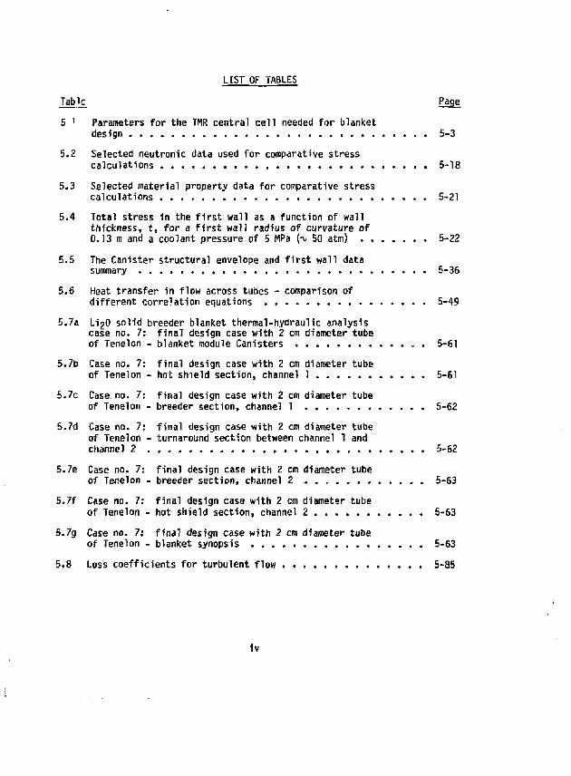
LIST OF TABLES Tabic Page 5 7 Parameters for the TMR central cell needed for blanket

design 5-3 5.2 Selected neutronic data used for comparative stress

calculations 5-18 5.3 Selected material property data for comparative stress

calculations 5-21 5.4 Total stress in the first wall as a function of wall

thickness, t, for a first wall radius of curvature of 0.13 m and a coolant pressure of 5 MPa ( 50 atm) 5-22

5.5 The Canister structural envelope and first wall data summary 5-36

5.6 Heat transfer in flow across tubes - comparison of different correlation equations 5-49

5.7a LigO solid breeder blanket thermal-hydraulic analysis case no. 7: final design case with 2 cm diameter tube of Tenelcn - blanket module Canisters . . . . . . 5-61

5.7b Case no. 7: final design case with 2 cm diameter tube of Tenelon - hot shield section, channel 1 5-61

5.7c Case. no. 7: final design case with 2 cm diameter tube of Tenelon - breeder section, channel 1 5-62

5.7d Case no. 7: final design case with 2 cm diameter tube of Tenelon - turnaround section between channel 1 and channel 2 5-62

5.7e Case no. 7: final design case with 2 cm dianieter tube of Tenelon - breeder section, channel 2 5-63

5.7f Case no. 7: final design case with 2 cm diametar tube of Tenelon - hot shield section, channel 2 5-63

5.7g Case no. 7; final design case with 2 cm diameter tube of Tenelon - blanket synopsis 5-63

5.8 Loss coefficients for turbulent flow , 5-85

iv

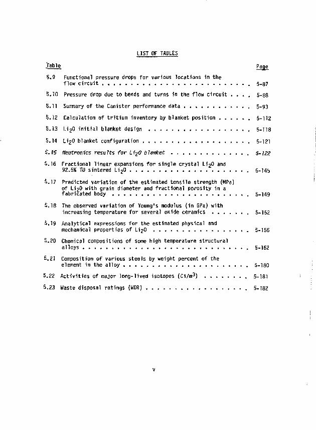
LIST OF TABLES .Table Page 5.9 Functional pressure drops for various locations in the

flow circuit 5-87 5.10 Pressure drop due to bends and turns in the flow circuit .... 5-88 5.11 Summary of the Canister performance data 5-93 5.12 Calculation of tritium inventory by blanket position 5-112 5.13 Li 20 initial blanket design 5-118 5.14 Li£0 blanket configuration 5-121 S. i5 iTeutronfcs results f a r tfgtf blanket 5-122

5.16 Fractional linear expansions for single crystal L12O and 92.5% TO sintered Li 20 5-145

5.17 Predicted variation of the estimated tensile strength (MPa) of LigO with grain diameter and fractional porosity in a fabricated body 5-149

5.18 The observed variation of Young's modulus (in GPa) with increasing temperature for several oxide ceramics 5-152

5.19 Analytical expressions for the estimated physical and mechanical properties of LigO 5-155

5.20 Chemical compositions of some high temperature structural alloys 5-162

5.21 Composition of various steels by weight percent of the element in the alloy 5-180

5.22 Activities of najor long-lived isotopes (Ci/m3) 5-181 5.23 Waste disposal ratings (WDR) . 5-182

v

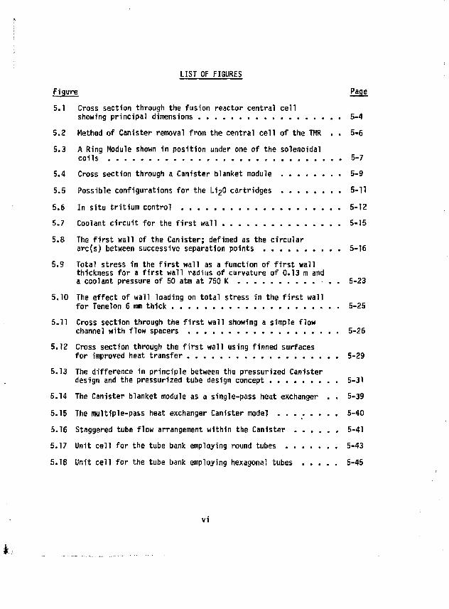
LIST OF FISURES Figure Page 5.1 Cross section through the fusion reactor central cell

showing principal dimensions 5-4 5.2 Method of Canister removal from the central cell of the TMR . . 5-6 5.3 A Ring Module shown in position under one of the solenoidal

coils . . . . . . . . . . . . . . . . . . . 5-7 5.4 Cross section through a Canister blanket module 5-9 5.5 Possible configurations for the LigO cartridges 5-11 5.6 In situ tritium control 5-12 5.7 Coolant circuit for the first wall 5-15 5.8 The first wall of the Canister; defined as the circular

arc(s) between successive separation points 5-16 5.9 Total stress in the first wall as a function of first wall

thickness for a first wall radius of curvature of 0.13 m and a coolant pressure of 50 atm at 750 K - . . 5-23

5.10 The effect of wall loading on total stress in the first wall for Tenelon 6 mm thick 5-25

5.11 Cross section through the first wall showing a simple flow channel with flow spacers 5-26

5.12 Cross section through the first wall using finned surfaces for improved heat transfer 5-29

5.13 The difference in principle between the pressurized Canister design and the pressurized tube design concept 5-31

5.14 The Canister blanket module as a single-pass heat exchanger . . 5-39 5.15 The multiple-pass heat exchanger Canister model , 5-40 5.16 Staggered tube flow arrangement within the Canister 5-41 5.17 Unit cell for the tube bank employing round tubes 5-43 5.18 Unit cell for the tube bank employing hexagonal tubes 5-45

vi

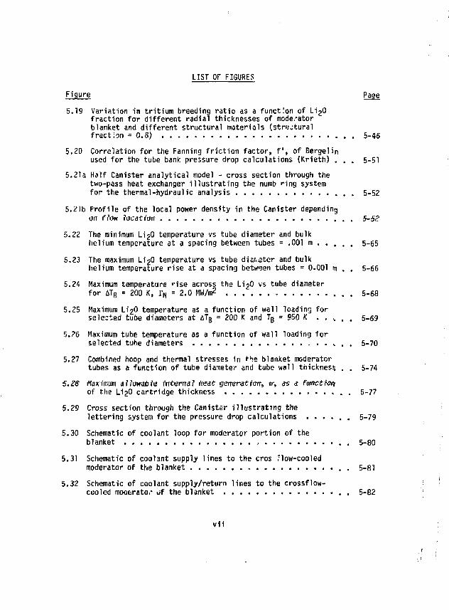
LIST OF FIGURES Figure Page 5.19 Variation in tritium breeding ratio as a function of LijO

fraction for different radial thicknesses of moderator blanket and different structural materials (structural fraction = 0.8) 5-46

5.20 Correlation for the Fanning friction factor, f, of Bergelin used for the tube bank pressure drop calculations (Krieth) . . . 5-51

5.21a Half Canister analytical model - cross section through the two-pass heat exchanger illustrating the numb >"ing system for the thermal-hydraulic analysis 5-52

5.21b Profile of the local power density in the Canister depending on f tow iacatran 5-52

5.22 The minimum U2O temperature vs tube diameter and bulk helium temperature at a spacing between tubes = .001 m 5-65

5.23 The maximum Li?0 temperature vs tube diar..eter and bulk helium temperature rise at a spacing between tubes = 0.001 hi . . 5-66

5.24 Maximum temperature •"ise across the L12O vs tube diameter for 6TB = 200 K, I'M = 2.0 MW/m2 5-68

5.25 Maximum LijO temperature as a function of wall loading for selected tube diameters at AT B = 200 K and T B = 950 K 5-69

5.26 Maximum tube temperature as a function of wall loading for selected tube diameters •. . . 5-70

5.27 Combined hoop and thermal stresses in the blanket moderator tubes as a function of tube diameter and tube wall thickness . . 5-74

5.28 ifaxratmr aftowafrfe frTCerrraF fte&t gerrerectftrrr, w, <rs <f f m c t i o t t of the LigO cartridge thickness * . . 5-77

5.29 Cross section through the Canister illustrating the lettering system for the pressure drop calculations . . . . . . 5-79

5.30 Schematic of coolant loop for moderator portion of the blanket „ . 5-8O

5.31 Schematic of coolant supply lines to the cros How-cooled moderator of the blanket , . 5-81

5.32 Schematic of coolant supply/return lines to the crossflow-cooled mooerato,* of the blanket . 5-82

vn

LIST OF FIGURES Figure Page 5.33 Schematic of coolant return lines from the crossflow-cooled

moderator of the blanket 5-83 5.34 Cross section through a typical helium transport pipe

showing insulation 5-90 5.35 End view representation of a LigO element on 14 urn centers

by a 12 nn diameter right circular cylinder 5-107 5.36 Li20 temperatures as a function of position in the blanket . . . 5-110 5.37 Tritium breeding ratio (TBP.) vs LigO volume fraction 5-119 5.38 Tritium breeding ratio (TBR) vs L12O thickness 5-120 5.39 Spatial distribution of power density ip U 2 O blanket 5-125 5.40 Spatial diitribut' n of tritium breeding in LigO blanket . . . . 5-126 5.41 Spatial distribution of atom displacement rate in Li^O

blanket 5-128 5.42 Spatial distribution of He production rate in Li^O blanket . . . 5-129 5.43 Spatial distribution of hydrogen production rate in Li^O

blanket 5-130 5.44 A lead zirconate/LijO blanket design 5-132 5.45 Spatial distribution of tritium breeding in an Li 20 blanket

with Z.r5Pb3 multiplier 5-133 5.46 Blanket energy/tritium breeding ratio trade-offs for

varying LljQ and multiplier thicknesses S-^34 5.47 Tritium breeding ratio (TBR) vs l.i20 volume fraction 5-136 5.48 Total blanket energy disposition vs tritiiffl breeding ratio

(TBR) for different structura1 materials --13B 5.49 The dependence of open and closed porosity in LigO as a

function of overall specimen density 5-141 5.50 Thermal conductivities of LigO as a function of

percentage of theoretical density and temperature 5-743

vm

LIST OF FIGURES Figure Page 5.51 A correlation of Knoop microhardness with tensile

strength for several oxide ceramics 5-147 5.52 The correlation of Young's modulus of elasticity with

melting point for cubic oxides and metals 5-150 5.53 Poisson's ratio as a function of temperature for several

oxides . , 5-156 5.54 Variation of the thermal stress factor M for Li 20 as a

function of temperature and porosity 5-157 5.55 Elastic modulus vs temperature for various high temperature

materials 5-161 5.56 Coefficient of thermal expansion vs temperature in some

high temperature materials . . . . . . . . 5-164 5.57 Thermal conductivity vs temperature for some high

temperature materials 5-165 5.58 Minimum expected yield strength vs temperature for several

high temperature materials . . . . . . . . 5-168 5.59 Minimum rijpture life in three years vs temperature for some

high temperature materials 5-171 5.60 Stress to produce 1.0% total strain in three years vs

temperature for some high temperature materials 5-173 5.61 Stress for- a three-year life vs temperature for various

vanadium <#,£ fasa all&ys , , , , , , , . . - , . , . 5-375 5.62 Swelling behavior of austenitic Fe-Cr-Ni, Fe-Cr-Mn-Ni, and

ferritic steels irradiated in various sources 5-177

ix

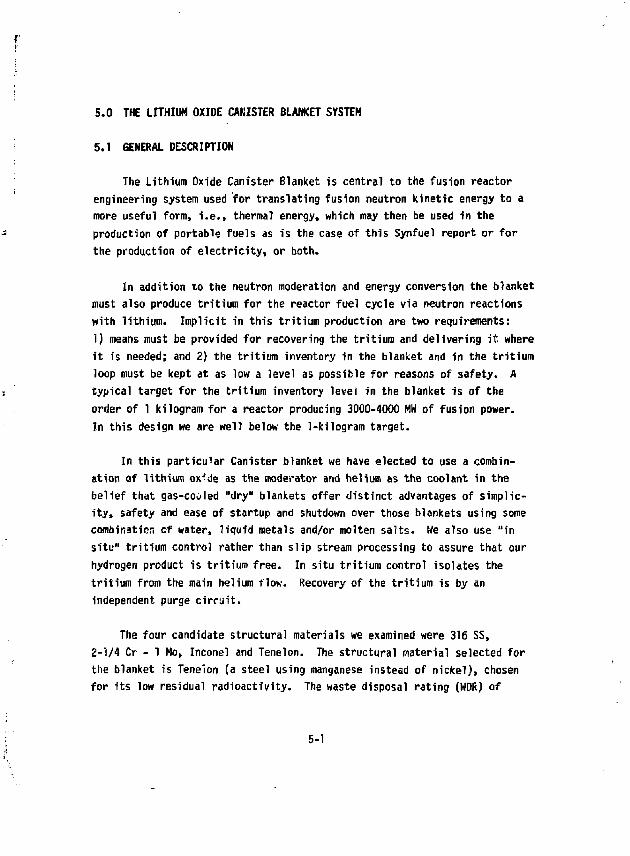
5.0 THE LITHIUM OXIDE CANISTER BLANKET SVSTEH

5.1 GENERAL DESCRIPTION

The Lithium Oxide Canister Blanket is central to the fusion reactor engineering system used for translating fusion neutron kinetic energy to a more useful form, i.e., thermal energy, which may then be used in the production of portable fuels as is the case of this Synfuel report or for the production of electricity, or both.

In addition to the neutron moderation and energy conversion the blanket must also produce tritium for the reactor fuel cycle via neutron reactions with lithium. Implicit in this tritium production are two requirements: 1) means must be provided for recovering the tritium and delivering it where it is needed; and 2) the tritium inventory in the blanket and in the tritium loop must be kept at as low a level as possible for reasons of safety. A typical target for the tritium inventory level in the blanket is of the order of 1 kilogram for a reactor producing 3000-4000 HH of fusion power. In this design we are well below the 1-kilogram target.

In this particular Canister blanket we have elected to use a combin­ation of lithium ox^de as the moderator and helium as the coolant in the belief that gas-cooled "dry" blankets offer distinct advantages of simplic­ity, safety and ease of startup and shutdown over those blankets using some combination cf water, liquid metals and/or molten salts. We also use "in situ" tritium control rather than slip stream processing to assure that our hydrogen product is tritium free. In situ tritium control isolates the tritium from the main helium flow. Recovery of the tritium is by an independent purge circuit.

The four candidate structural materials we examined were 316 SS, 2-1/4 Cr - 1 Mo, Inconel and Tenelon. The structural material selected for the blanket is Tenelon (a steel using manganese instead of nickel), chosen for its low residual radioactivity. The waste disposal rating (WDR) of

5-1

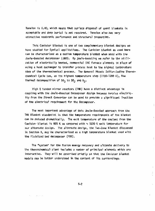
Tenelon is 0.40, which means that surface disposal of spent blankets is acceptable and deep burial is not required. Tenelon also has very attractive neutronic performance and structural properties.

This Canister blanket is one of two complementary blanket designs we have studied for Synfuel applications. The Canister blanket as used here can be characterized as a medium temperature blanket when used with the Joule-Boosted decomposer (JBO). By joule-boosting we refer to the utili­zation of electrically heated, commercial SiC furnace elements in place of using a heat exchanger to transfer process heat to the highest temperature step of the thermochemical process. The General Atomic Sulfur-Iodine Thermo chemical Cycle has, as its highest temperature step {1100-1200 K), the thermal decomposition of S0 3 to S0~ and 0,.

High Q tandem mirror reactors (TMR) have a distinct advantage in coupling with the Joule-Boosted Decomposer design because surplus electric­ity from the Direct Converter can be used to provide a significant fraction of the electrical requirement for the Decomposer.

The most important advantage of this Joule-Boosted approach from the TMR Blanket standpoint is that the temperature requirements of the blanket can be reduced dramatically. The exit temperature of the coolant from the Canister blanket is 825 K as compared with ^ 1200 K exit temperature for our alternate design. The alternate design, the Two-Zone blanket discussed in Section 6, may be characterized as a high temperature blanket used with the fluidized bed decomposer (FBD).

The "system" for the fusion energy recovery and ultimate delivery to the thermochemical plant includes a number of principal elements which are interactive. They will be described briefly so that the Canister blanket module may be better understood in the context of its surroundings.

5-2

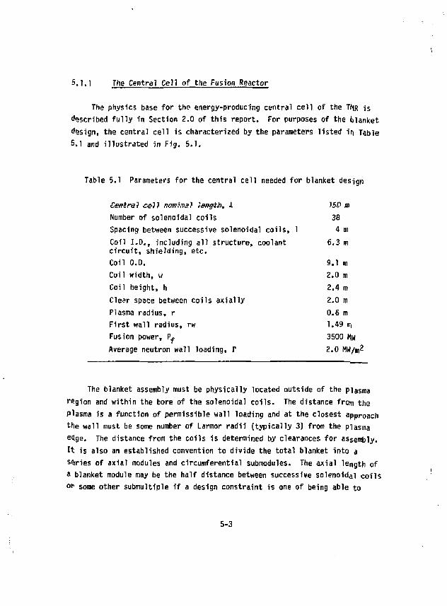
5.1.1 The Central Cell of the Fusion Reactor

The physics base for the energy-producing central cell of the TMR is described fully in Section 2.0 of this report. For purposes of the blanket design, the central cell is characterized by the parameters listed ir> Table 5,1 and illustrated in Fig. 5.1.

5.1 Parameters for the central cell needed for blanket design

£&?tral £•#?? iTCWJiTO? t&tgtb, I JBD x»

Number of solenoidal coils 38 Spacing between successive solenoida coils, 1 4 m Coil I.D., including all structure, circuit, shielding, etc.

:oolant 6.3 m

Coil O.D. 9.1 m Coil width, w 2.0 m Coil height, h 2.4 m Clear space between coils axially 2.0 m Plasma radius, r 0.6 m First wall radius, rw 1.49 rr, Fusion power, P- 3500 hW Average neutron wall loading, r 2.0 MH/ m2

The blanket assembly must be physically located outside of the plasma region and within the bore of the solenoidal coils. The distance from the plasma is a function of permissible wall loading and at the closest approach the wall must be some number of Larmor radii (typically 3) from the plasma edge. The distance from the coils is determined by clearances for assembly. It is also an established convention to divide the total blanket into a series of axial modules and circumferential submodules. The axial length of a blanket module may be the half distance between successive solenoidal coils or* some other submultiple if a design constraint is one of being able to

5-3

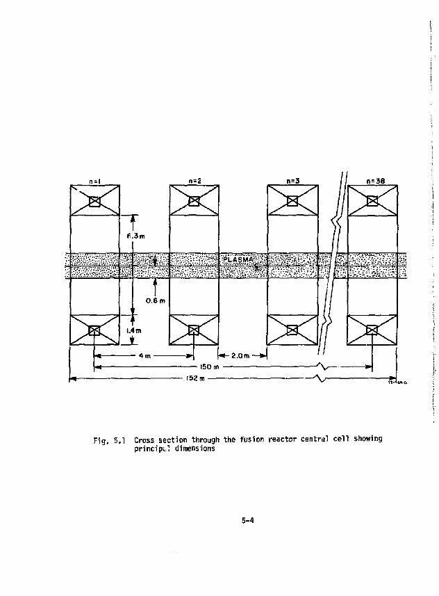
n=38

Fig. 5,1 Cross section through the fusion reactor central cell showing principal dimensions

5-4

leave the coils in place when blanket installation or removal is required. This is a highly practical consideration and one adopted here since the superconducting solenoidal coils and all their associated circuitry are generally designed for the life of the plant ( 30 years), whereas blanket module life expectancy is limited to approximately 3 to 5 years.

Figure 5.2 illustrates, in a highly schematic way, the principle of module placement or removal for the blanket design to be discussed in this section. Module A, shown in place, is installed by a vertical motion to the reactor ([, followed by an axial translation placing it partially under the solenoid. Module B, a mirror inage of A, is shown partially installed and need only be lowered to the reactor Q^to be in place. Structural supports between the fixed solenoidal coils are spaced so that vertical placement or removal of the blanket can be accommodated. Ring manifold piping is separately installed after the ring module is in place.

5.1.2 The Axial Blanket Module - The "Ring" Modules Within the Central Cell

The central cell is filled with a number (75) of ring modules arranged in series axially along the 150-m central cell. The ring module is illus­trated in Fig. 5.3. One ring module occupies the half space between the solenoidal coils. Module A, as Fig. 5.2 indicated, is partially under the solenoid, while module B lies in the free space between coils. The modules are exactly identical, one being turned 180 degrees with respect to the other. The ring manifolding transfers the coolant (helium) to the supply and return headers located outboard of the solenoidal coils. The set of four header circuits run longitudinally along the length of the central cell and terminate in a set of intermediate steam-generator heat exchangers (IHX) that are located as close7y as possible to the fusion reactor but is isolated by protective concrete wall barriers.

Radially inward from the ring headers the cold shield forms the support structure for both the ring headers and the moderating blanket/hot shield.

5-5

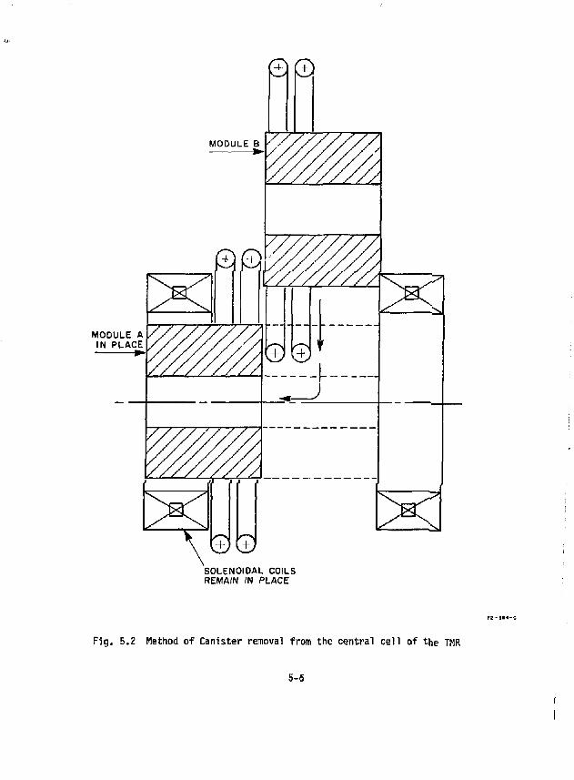
0

MODULE B

SOLENOIDAL COILS REMAIN IN PLACE

Fig. 5.2 Method of Canister removal from the central ce l l of the TMR

5-6

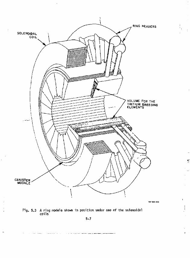
RING HEADERS

SOLENOIDAL i COIL

CANISTER MODULE

VOLUME FOR THE TRITIUM BREEDING ELEMENTS

Fig. 5.3 A ring module shown in position under one of the solenoidal coils

5-7

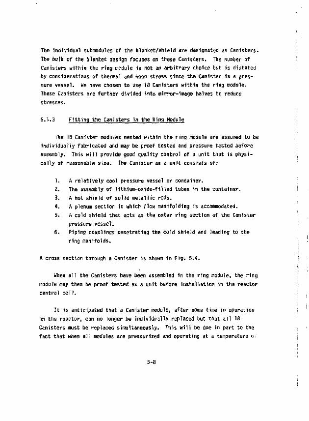
The individual submodules of the blanket/shield are designated as Canisters. The bulk of the blanket design focuses on these Canisters. The number of Canisters within the ring mrdule is not an arbitrary choice but is dictated by considerations of thermal and hoop stress since the Canister is a pres­sure vessel. We have chosen to use IS Canisters within the ring module. These Canisters are further divided into mirror-image halves to reduce stresses.

5.1.3 Fitting the Canisters in the Ring Module

The 18 Canister modules nested within the ring module are assumed to be individually fabricated and may be proof tested and pressure tested before assembly. This will provide good quality control of a unit that is physi­cally of reasonable size. The Canister as a unit consists of:

1. A relatively cool pressure vessel or container. 2. The assembly of lithium-oxide-filled tubes in the container. 3. A hot shield of solid metallic rods. 4. A plenum section in which flow manifolding is accommodated. 5. A cold shield that acts as the outer ring section of the Canister

pressure vessel. 6. Piping couplings penetrating the cold shield and leading to the

ring manifolds.

A cross section through a Canister is shown in Fig. 5.4.

When all the Canisters have been assembled in the ring module, the ring module may then be proof tested as a unit before installation in the reactor central cell.

It is anticipated that a Canister module, after some time in operation in the reactor, can no longer be individually replaced but that all 18 Canisters must be replaced simultaneously. This will be due in part to the fact that when all modules are pressurized and operating at a temperature c:

5-8

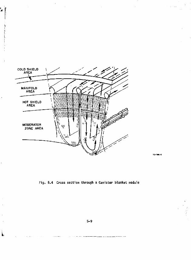
COLD SHIELD AREA

Fig. 5.4 Cross section through a Canister blanket module

5-9

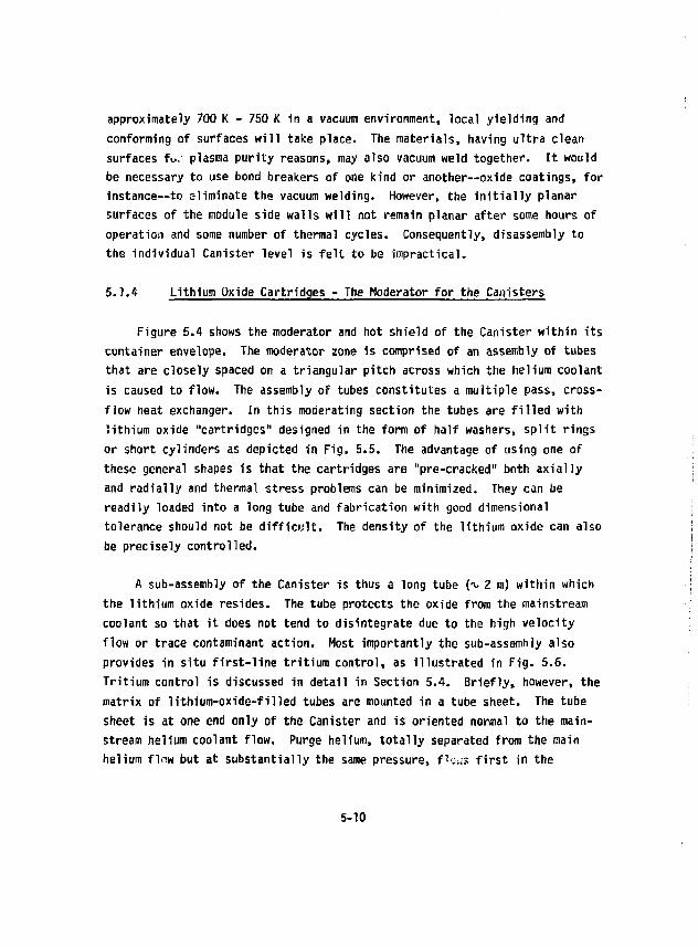
approximately 700 K - 750 K in a vacuum environment, local yielding and conforming of surfaces will take place. The materials, having ultra clean surfaces fu. plasma purity reasons, may also vacuum weld together. It would be necessary to use bond breakers of one kind or another—oxide coatings, for instance—to eliminate the vacuum welding. However, the initially planar surfaces of the module side walls will not remain planar after some hours of operation and some number of thermal cycles. Consequently, disassembly to the individual Canister level is felt to be impractical.

5.1.4 Lithium Oxide Cartridges - The Moderator for the Canisters

Figure 5.4 shows the moderator and hot shield of the Canister within its container envelope. The moderator zone is comprised of an assembly of tubes that are closely spaced on a triangular pitch across which the helium coolant is caused to flow. The assembly of tubes constitutes a multiple pass, cross-flow heat exchanger. In this moderating section the tubes are filled with lithium oxide "cartridges" designed in the form of half washers, split rings or short cylinders as depicted in Fig. 5.5. The advantage of using one of these general shapes is that the cartridges are "pre-cracked" both axially and radially and thermal stress problems can be minimized. They can be readily loaded into a long tube and fabrication with good dimensional tolerance should not be difficult. The density of the lithium oxide can also be precisely controlled.

A sub-assembly of the Canister is thus a long tube ( 2 m) within which the lithium oxide resides. The tube protects the oxide from the mainstream coolant so that it does not tend to disintegrate due to the high velocity flow or trace contaminant action. Host importantly the sub-assembly also provides in situ first-line tritium control, as illustrated in Fig. 5.6. Tritium control is discussed in detail in Section 5.4. Briefly, however, the matrix of lithium-oxide-filled tubes are mounted in a tube sheet. The tube sheet is at one end only of the Canister and is oriented normal to the main­stream helium coolant flow. Purge helium, totally separated from the main helium flow but at substantially the same pressure, fle.;s first in the

5-10

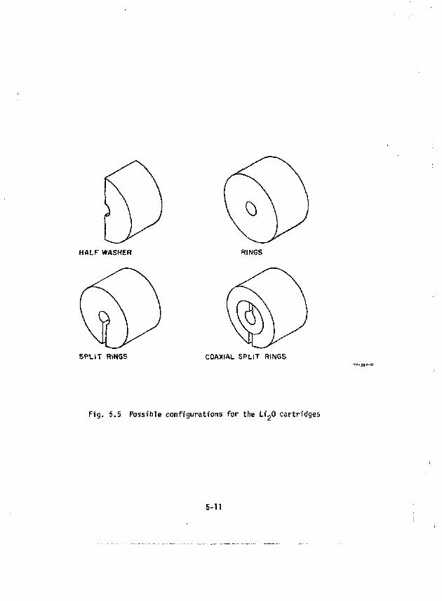
HALF WASHER RINGS

SPLIT RINGS COAXIAL SPLIT RINGS

Fig. 5.5 Possible conf igurat ions fo r the L i ? 0 cartr idges

5-11

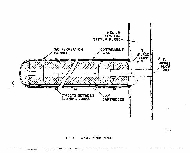
HELIUM FLOW FOR

TRITIUM PUR6E-

,SiC PERMEATION BARRIER

CONTAINMENT TUBE

tnwwwmm»»a

SPACERS BETWEEN AJOINING TUBES

L i £ 0 CARTRIDGES

Fig. 5.6 In situ tritium control

annular spac«> between the tube wall and the Li„0 cartridge and then returns through the central hole in the cartridge. The mass flow of this helium used to purge the tritium is very low and inconsequential compared to the main­stream coolant flow.

In the hit shield zone of the Canister the tubes are replaced by solid rods. In the casis that were studied for the Canister tnermal-hydraulie performance, ail tubes and rods were assumed to be the same diameter. This need not be the case nor is it necessary to have all moderating tubes the same diameter. In fact, tubes could progressively increase in diametr, as a function of increasing blanket radius to partially compensate for the exponentially decreasing energy deposition. For this particular study we concentrated masnly on sizing the tubes to match overall neutronics/thermal-hydraulic needs and have not as yet used the second order refinement of having graded sizes.

5-13

5.2 THE CANISTER FIRST WALL AND STRUCTURAL ENVELOPE—THE "COOL" CONTAINER

The Canister structural container is an independently cooled, double-walled envelope surrounding the lithium-oxide-moderating medium and the hot shield. The coolant circuit for the first wall is shown in Fig. 5.7. High pressure helium enters the Canister at its cen1;erline at a temperature of 525 K, flows radially inward to the first wall where the flow divides equally, flowing outward in an enveloping flow around the Cfliister module to collecting plenums. The helium exit temperature is 625 K. The pressure of the first wall helium coolant circuit is in the range of 40 to 60 atmo­spheres, dictated by the pressure of the mainstream coolant flow, to which it is set equal, and further dictated by the need to have highly efficient heat transfer in the first wall. From 5 to 15% of the total blanket energy can be deposited in the first wall. The helium temperature and flow rate is selected so as to limit the maximum material temperature in the first wall structural envelope to approximately 750 K. This maximum material temper­ature is chosen to limit radiation damage (discussed in Section 5.6 on materials) and to stay below the threshold of creep behavior so as to design for stresses based on yield strength. The principal stress in the first wall is a membrane stress arising because the Canister is a pressure vessel with a first wall curved surface subjected to hoop stress. Thermal stresses also occur due to heat removal from one side only of the first wall. The thermal stresses are additive to the hoop stresses at the inner surface of the first wall.

5.2.1 Stresses in the First wall of the Canister Blanket Module

For our reference design we have assumed that there are 18 Canisters or blanket submodules in a ring module. We have further assumed that the indi­vidual modules bear one against the other circumferentially until a point is reached where they separate. The first wall of any one Canister is defined as the curved surfr.ce that exists between successive separation points. The first wall and its separation points are depicted in Fig. 5.8A and B.

5-14

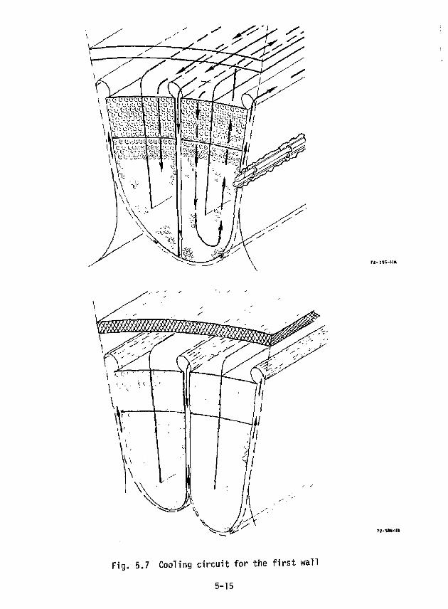
Fig, 5,7 Cooling circuit for the first wall

5-15

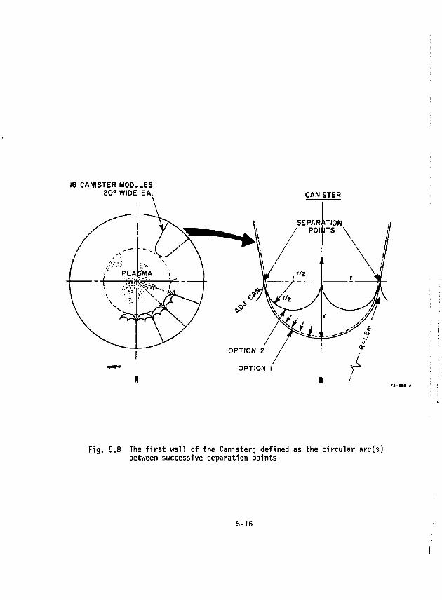
18 CANISTER MODULES 20° WIDE EA. CANISTER

Fig. 5.8 The first wall of the Canister; defined as the circular arc(s) between successive separation points

5-16

5.2.2 Hoop Stresses Due to Pressure Loading

At the point of separation of the curved first wall from the side walls, eac.'' module has a circular arc first wall of some radius, r. The value of r will determine the hoop stress in the first wall. The stresses arise because the blanket module is a pressure vessel operating at a pressure, P. The reference design pressure is 50 atm.

We take 7.5 meters as the distance f:osi the plasma centerline to the separation point of the first we77. The least value of r for a circular arc first wall for the entire Canister (option 1 in Fig. 5.7) is when the arc is a half circle. For the half circle:

r " T8TT " °-26 " This least value r yields the lowest stress from the simple hoop stress

equation:

The least value of r also minimizes any bending stresses that occur at the separation point between first wall and side wall.

There is no dlscemable advantage in increasing the radius of curvature of the first wall in order to move the point of closest approach of the first wall away from the plasma. The small decrease in wall loading that results cannot compensate for the increased level of stresses due both to hoop stress and to the bending stress introduced near the separation point. If the stresses were quite low then the situation might he different. Such is not the case and therefore we not only used the least value of r but also looked to other means of lowering the hoop stress since* when it was combined with the thermal stress, we found the allowable design stress to be exceeded. Referring back to Figs. 5.7 and 6.8, it may be noted that two options for the first wall radius are shown. Option 1, where r * 0.26 m, has just been discussed. As a straightforward means of decreasing stress, option 2

5-17

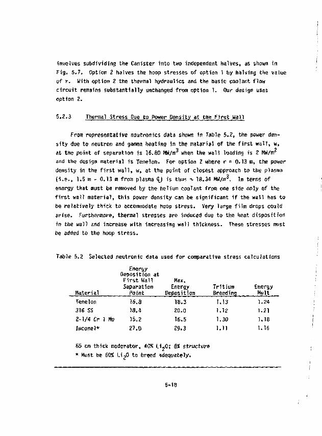
involves subdividing the Canister into two independent halves, as shown in Fig. 5,7. Option 2 halves the hoop stresses of option 1 by halving the value of r. With option 2 the thermal hydraulics and the basic coolant flow circuit remains substantially unchanged from option 1. Our design uses option 2.

5.2.3 Thermal Stress Due to Power Dejisity at the .First Wall

From representative nautronics data shown in Table 5.2, the power den­sity due to neutron and gamma heating in the material of the first wall, w, at the point of separation is 16.80 MW/irr when the wall loading is 2 MW/irr and the design material is Tenelon. For option H where r s 0.13 m, the power density in the first wall, w, at the point of closest approach to the plasma (i.e., 1.5 in - 0.13 BI from plasma <{.) is thu< -v 18.34 MW/m3. In tenre of energy that must be removed by the helium coolant from one side only of the first wall material, this power density can be significant if the wall has to be relatively thick to accommodate hoop stress. Very large film drops could arise. Furthermore, thermal stresses are induced due to the heat disposition in the wall and increase with increasing wall thickness. These stresses must be added to the hoop stress.

Table 5.2 Selected neutronic data used for comparative stress calculations Energy

Deposition at First Wall Max. Separation Energy Tritium Energy

Material Point Deposition Breeding Mult Tenelon 16.8 18.3 1.13 1.24 316 SS 18.4 20.0 1.12 1.21 2-1/4 Cr 1 Mo 15.2 16.5 1.30 1.18 Inconel* 27.0 29.3 1.11 1.16

65 cm thick moderator, 4CS Li-O; 8% structure * Must be 6 W Li~0 to breed adequately.

5-18

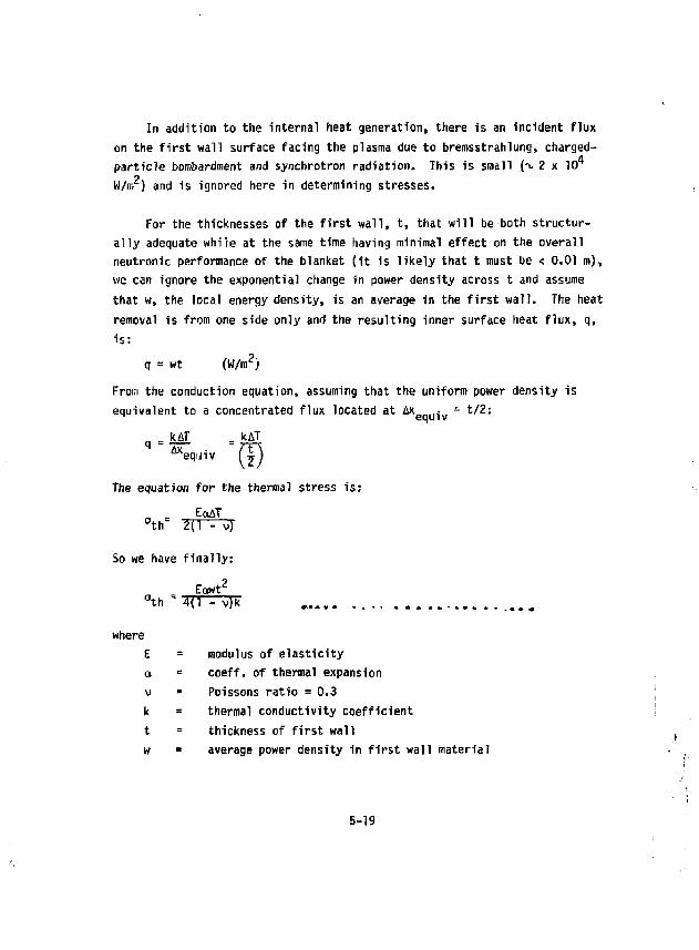
In addition to the internal heat generation, there is an incident flux on the first wall surface facing the plasma due to bremsstrahlung, charged-particle bombardment and synchrotron radiation. This is small K Z x 10^ W/m Z) and is ignored here in determining stresses.

For the thicknesses of the first wall, t, that will be both structur­ally adequate while at the same time having minimal effect on the overall neutronic performance of the blanket (it is likely that t must be < 0.01 m ) , we can ignore the exponential change in power density across t and assume that w, the local energy density, is an average In the first wall. The heat removal is from one side only and the resulting inner surface heat flux, q, is:

q = wt (W/m 2) From the conduction equation, assuming that the uniform power density is equivalent to a concentrated flux located at ^gnui,, = t/ 2 :

q"«.q.i1v '(f) The equation for the thermal stress is:

. EoAT ath" 2(1 - v)

So we have finally:

Eawt 2

°th " 4(1 - v)k

where E = modulus of elasticity a = coeff. of thermal expansion v = Poissons ratio = 0.3 k = thermal conductivity coefficient t = thickness of first wall w = average power density in first wall material

5-19

Example: For t • 0.01 m using a familiar structural material such as 316

stainless steel

„ _ 1.65 x 10 1 1 x 20 x 10~ 6 x 20.0 x 10 6(.O1) 2

aTH 4(1 - 0.3J 17

= 138 MPa = 20000 psi

For structural materials with much higher strength than 316 SS, such as Inconel fiOOH, the thermal conductivity is higher (24 vs 17), the coefficient of expansion is lower (17 vs 20), but the local internal heat generation is much higher (29.3 w/cm vs 20.0) due to the high nickel content of the alloy. The resulting thermal stresses are slightly lower for the Inconel than for the 316 SS, "v 127 HPa for the example cited.

Tor Tenelon, our choice for the first wall material, optimum for its low residual radioactivity and minimal waste disposal problems, the thermal stress level is the lowest of the materials considered~78 HPa for the same example. This low stress is <?ue to both lower internal heat generation and a thermal conductivity that is reasonably high. The 2-1/4 Cr Mo provides an attractive alternate but has a higher waste disposal rating (WDR) (15 vs 0.4 for the Tenelon). The WDR is the dilution factor that must be used in dis­poning of the spent material. For instance, a WDR of 15 means that 15 m 3

o. inert diluent would have to be added to 7 m of spent materia? and the total then homogenized and sealed in containers for acceptable disposal.

Complete property data for all four materials can be found in the appropriate subsection. T*ble 5.3 provides the data required here for the thermal stress calculations. The data are at 750 K.

5-20

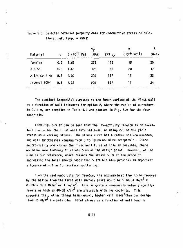
Table 5.3 Selected material property data for comparative stress calcula­tions, ref. temp. = 750 K

ay a k Material v E {lO^ Pa) (MPA) 2/3o y (10"6 °C"1) (W-K)

Tenelon 0.3 1.65 275 175 18 25 316 SS 0.3 1.65 125 83 20 17 2-1/4 Cr 7 Mo 0.3 1.80 205 137 15 32 Inconel 800H 0.3 1.72 900 597 17 24

The combined tangential stresses at the inner surface of the first wall as a function of wall thickness for option 2, where the radius of curvature is 0.13 m, are compiled in Table 5.4 and plotted in Fig. 5.9 for the four materials.

From Fig. 5.9 it can be seen that the low-activity Tenelon is an excel­lent choice for the first wall material based on using 2/1 of the yield stress as a working stress. The stress curve has a rather shallow minimum, and wall thicknesses ranging from 5 to 10 mm would be acceptable. Since neutrom'cally one wishes the first wall to be as thin as possible, there would be some tendency to choose 5 mm as the design point. However, we use 6 mm as our reference, which lessens the stress •>• 85, at the price of increasing the local energy deposition ^ 17X but also provides an important allowance of ^ 1 mm for surface sputtering.

From the neutronic data for Tenelon, the maximum heat flux to be removed by the helium from the first wall surface (max) would be -v 18.34 MW/m3 x 0.006 = 0.11 MW/nr or 11 w/cnr. This is quite a reasonable value since flux levels as high as 40-50 w/cm are plausable with gas cool-^ts. This suggests that, other things being equal, higher wall loads'than our design level Z MW/m are possible. Total stress as a function of wall load is

5-21

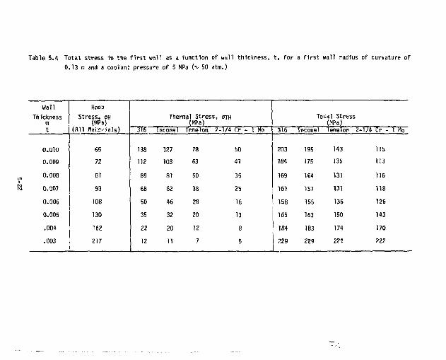
Table 5.4 Total stress in the first wall as a function of wall thickness, t, for a first wall radius of curvature of 0.13 m and a coolant pressure of 5 MPa ( 50 atm.)

Wall Hoop Thickness

m Stress, OH

(MPa) (All HatCiials)

Thermal Stress, OTH (MPa)

Total Stress (NPa)

t Stress, OH

(MPa) (All HatCiials) 316 [nconel Tenelon 2-1/4 Cr - 1 Mo 316 Inconel Tenelon 2 -1/4 Cr - 1 Ho

0.010 65 138 127 78 50 203 195 143 115 0.009 72 112 103 63 41 184 175 135 113 0.008 81 88 81 50 35 169 164 131 116 0.007 93 68 62 38 25 151 157 131 118 0.006 108 50 46 28 18 158 155 136 126 0.005 130 35 32 20 13 165 163 150 143 .004 162 22 20 12 8 184 183 174 170 .003 217 12 11 7 5 229 229 224 222

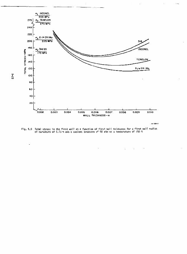
crv INCONEL 900 MPa

275 I o-y TENELON •S 275 MPa

240 (-

220

200

180

160

140

120

100

80

60

40

20

kA-L-0.003 0.004 0.005 0.006 0.007

WALL THICKNESS-m 0.00S 0.009

F ig . 5.9 Total stress i n the f i r s t wal l as a func t ion o f f i r s t wa l l th ickness f o r a f i r s t wa l l radius of curvature o f 0.13 m and a coolant pressure o f 50 atm at a temperature of 750 K

plotted in Fig. 5.10. The acceptable design stress, 2/3 the yield stress, is not reached until the wall loading is 5.0 MW/m . This is a very favorable Situation. The effect of wall loading on the heat transfer in the canister moderating volume is discussed in Section 5.3. Here it will be seen also 2 that wall loadings substantially higher than our 2 MW/m are feasible.

<>.2.4 Material Temperature at the First Hall

To optimize the interfacing oi the overall reactor blanket modules with the thermochemical plant (see Section 10 for details), the following specific design parameters were chosen for the wall coolant circuit:

o Coolant - helium o Inlet temperature, Tgj N = 525 K o Outlet temperature, T g 0 U T = 625 K o Coolant pressure, P = 50 atm o First wall is independently and integrally cooled o A quasi-adiabatic surface is assumed to exist between the first

wall coolant circuit and the main body of the moderating blanket o Wall thickness = 0.006 m

With these data and one further simplifying assumption, it is possible to closely estimate the maximum material temperature in the first wall- The approximation is that all energy deposition occurs in the curved surface of tbfi f ir^t DW.U if lewjtlk, «. = Q~13. *. i = 0*4.1. w,, vi ttwA, esseiKti&Uy w* energy deposition takes place in the lead-in and lead-out lengths. The annular spacing, 6, between the first wall and the adiabatic surface forms the cooling channel. This channe7 is kept intentionally small to enhance heat transfer. Flow spacers can be provided as illustrated in Fig. 5.11-The hydraulic diameter of this channel is 2 6.

The quantities to be determined in arriving at the material temperature are:

a) The energy to be removed

5-24

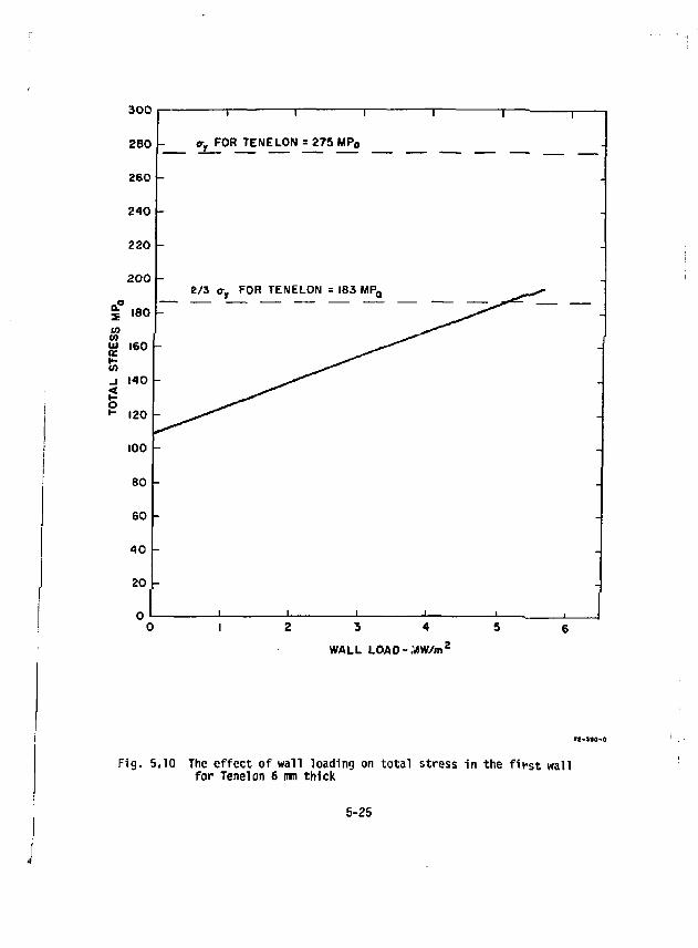
300

280

260

240

220

2001-

£ 180 -

100

80

60

40

20

O

<r, FOR TENELON = 275 MP„

2/3 cr. FOR TENELON = 183 MP„

3 4

WALL L0AD-.VW/m 2

Fig. 5.10 The effect of wall loading on total stress in the first wall for Tenelon 6 mm thick

5-25

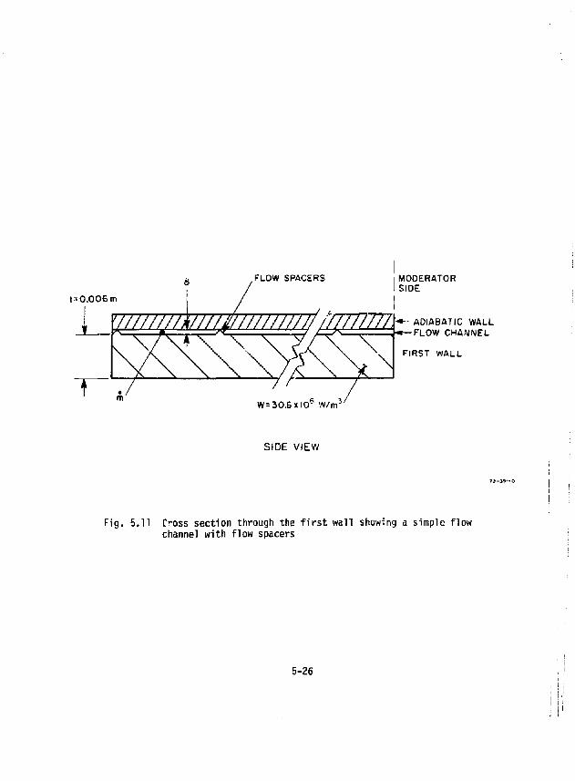
t--0.0 06 m

MODERATOR SIDE

ADIABATIC WALL -FLOW CHANNEL

FIRST WALL

W = 30.&xl0 6 W/m 3 /

SIDE VIEW

Fig. 5.11 f-oss sect ion through the f i r s t wal l showing a simple f low channel wi th f low spacers

5-26

%IIT = w U = 1 8 ' 3 4 * 1 ( ) 5 X ° ' 0 0 6 ' , 4 1 = 4 5 ' 1 1 6 w / " l WIDTH

b) The mass flow rate

m = - S _ = 45,116 C p A T B 5.2 x 103 x 100

= 0.085 kg/s (per mete, of widthi

c) The average flow velocity assuming flow gap & = 0.002 m

- in 0.085 , n 1 0 , u = ^ s 0.002(4.18) - ™-18ni/s

**"* ' - Jf - a r a ^ - * M **** J) The average Reynolds number, based on the hydraulic diameter, is

^ = 26l?(p) = .004 x 10.18(4.18) = 5 6 7 6

u 300 x 10* 7

To determine the average film coefficient, h, we may use the correlating equation:

N u = _ H = 0.023(Re)°- 8(Pr) 0 , 3 3

= .023 (5676)°* 8(.67) 0 - 3 3 = 20.3

T- _ 20.3 x 0.233 _ , , „ X,,J.V * O o l 1183 w/mK

Finally, with a heat f lux, q» equal to 18.34 x 106 x .006 = i . io x 105

W/m we obtain

AT - 1-1Q x 10S _ Q , ,, ATFILM " TTal 9 3 K

5-27

The temperature drop across the wall is

AT - al - i.i x io 5 * .006 . „ , K

The maximum material temperature is thus: TMAX = TB0UT + A TFILM + A TWALL

= 625 + 9 3 + 1 3 * 731 K

The film temperature drop of 93 K is somewhat high but acceptable since the material temperature of 731 K is well below a design limit of 823 K impeded by radiation damage considerations and Tow enough to be below the creep stress regime. However, it is desirable to reduce the film tempera­ture drop as much as is reasonably possible and one method for doing this is to resort to a grooved first wall design. The grooved first wall increases the area available for heat transfer and decreases the average inner surface flux, q. The complication, beyond that of having introduced a first wall that is more costly and difficult to fabricate, has to do with enhancing the heat transfer by making the first wall into a finned surface as shown in Fig. 5.12 results in the hydraulic diameter of the finned surface being intrinsically less than the hydraulic diameter for a simple gap. When the same flow velocity is retained, the Reynolds number thus decreases and tends to offset somewhat the surface area gain made by introducing the fin. Figure 5.12 illustrates a rough optimum for the fin proportions where the fin height (equal to its width) is equal to two-thirds of t.

5.2.5 Conclusions on the Stresses in the First Wall

It is important to note that the stresses in this curved first wall sheet are purely tensile membrane stresses and local thermal stresses. There are no bending stresses that can be caused by the pressure-vessel-type load­ing (except at the ends where a transition is made from the first wall to the end walls or from the first wall to the side walls). Therefore there is no

5-28

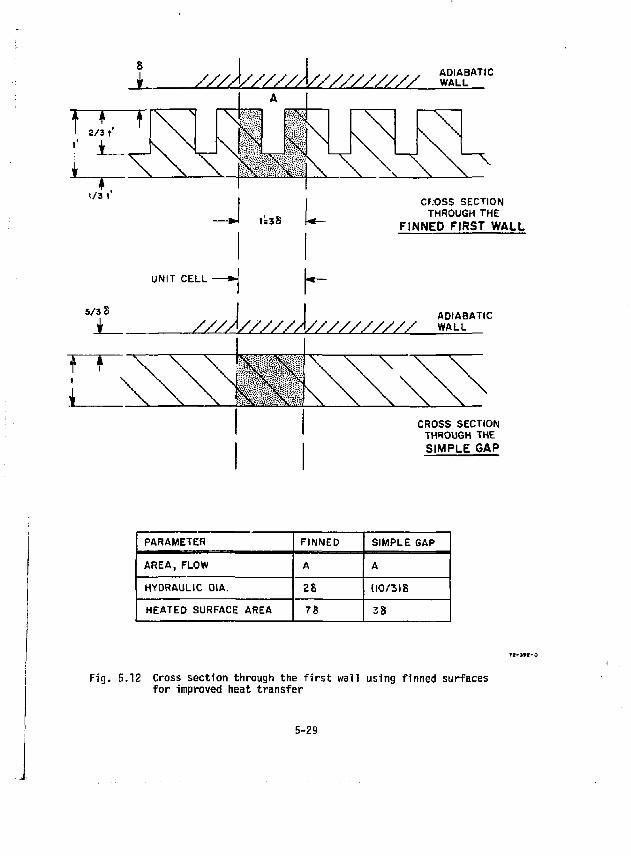
A ///A/////A////////// g"11

J t=3S U— CF:OSS SECTION

THROUGH THE FINNED FIRST WALL

5/3 S

1_

UNIT CELL \ -

'A/////X ADIABATIC ///A/////A////////// WALL

CROSS SECTION THROUGH THE SIMPLE GAP

PARAMETER FINNED SIMPLE GAP

AREA, FLOW A A

HYDRAULIC OIA. 26 110/3)8

HEATED SURFACE AREA 78 38

Fig. 5.12 Cross section through the f i r s t wall using f inned surfaces f o r improved heat t ransfer

5-29

additional strength benefit to be derived by adding fins for stiffening since th^re is no moment of inertia term in the hoop stress equation or in the thermal stress equation. The fins do help the heat transfer as was just inqicated. However, our choice for the first wall design is the flat plate with the uniform flow gap, based mainly on its simplicity, its structural adequacy and the fact that it is tolerant of wall loads as high as 5 Mw/m 2.

5-3.6 Comparison with an Alternate Canister Design

The first wall presents a significant but manageable stress problem as ft fs present ty corrffgurea'. if it sitarfa" prove ctes irab?e to depart from the pressurized, curved sheet approach presently used (actually the Canister is two coaxial curved sheets separated by a cooling space) then the way the module is pressure loaded must be changed. A possibility may appear t 0 exist of making the curved sheets into a tube array where the tube radius would be a Characteristic dimension for hoop stress caused by first wall coolant (Fig. 5.13). However, the pressure loading from the mainstream coolant flow would still create a hoop stress on the tubes which is still determined by the radius of curvature of the first wall. Thust in order to unload this pressure from the Canister first wall so as to decrease the stress, it would he necessary to flow the mainstream coolant within tubes that pass through the solid Li-O moderator rather than having the Li-O on the inside of the tubes and the flow on the outside.

Figure 5.13 illustrates the main differences in principle between the pressurized Canister design concept and the pressurized tube design concept. The pressurized tubes making up the first wall must be welded continuously, one to the next, presenting additional problems of structural integrity and first wall life.

It is our contention that the pressurized Canister design is a much setter choice than the pressurized tube design. The only proviso is that the structural envelope (the cool container) comprising the pressurized Canister must be independently cooled and held at modest temperatures as we havs done.

5-30

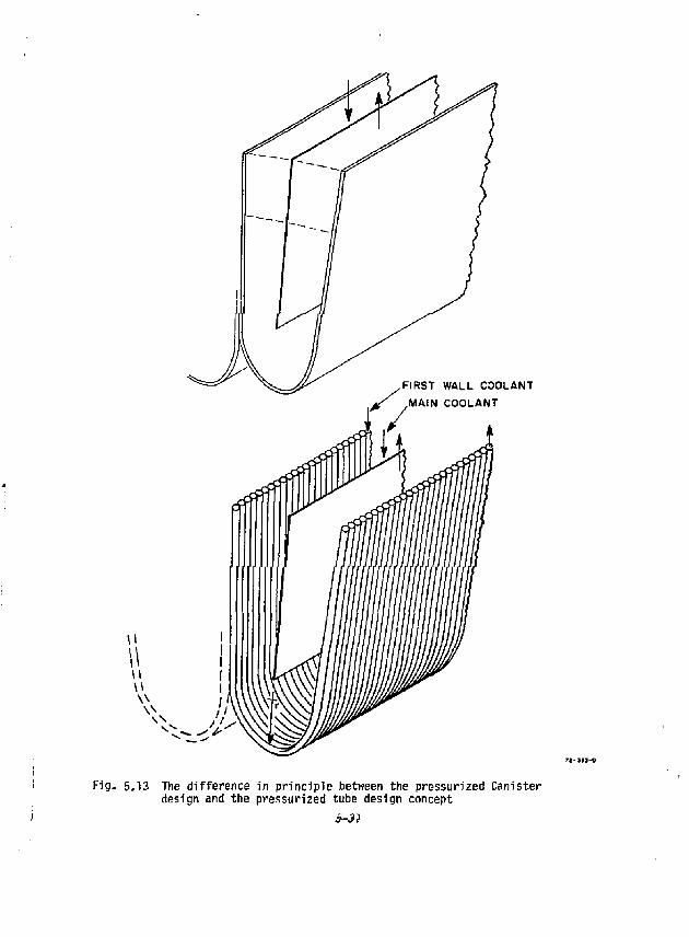
FIRST WALL COOLANT MAIN COOLANT

Fig- 5.13 The difference in principle between the pressurized Canister design and the pressurized tube design concept

j-JJ

With the pressurized Canister design concept, the helium pressure across the tubes containing the LigO in the moderator zone can be balanced. Even though the tube temperatures are high, the stresses are very low because of the pressure balancing. With the non-pressurized Canister the pressurized tubes in the moderator zone have relatively high hoop stresses which cannot be accommodated at high temperatures without resorting to materials that are much less desirable than Tene'on for low residual radioactivity.

5.2,7 Coolant Pressure Drop and Pumping Power in the First Wall

The frictional pressure drop in the first wall is given by the equation:

The Oarcy-Weisbach friction factor, f, for flow between parallel plates may be obtained from (Ref. Rohsenow & Hartnrtt, Handbook of Heat Transfer -McGraw Hill):

f = 0.316 ( R e ) " 0 , 2 5

(6000 < Re < 300,000) The turning loss where the flow divides at the first wall is:

*Pt * 4 - * KL where K^ = loss coefficient = 1.0,

For the reference c<se we have:

f = 0.316(5676) - 0 - 2 5 » 0.0365 Lp « 2.5 m = flow length D H = 0.004 W = Canister axial length = 2 m

S-32

APT 0 T - iP f + tPt - 0.0365 ^ g J O M

+ ( i s i a x z i o s i a i ) x K O

= 4941 + 217 = 5158 Pa (< 1. psi)

where we have neglected the small acceleration pressure drop, and where entrance and exit losses are accounted for elsewhere.

The pumping power per Canister half module, the pressure drop times the volumetric flow rate, is:

PP = AP T 0 T(Au)

= 5158(2 x 0.002 x 10.18) = 210 W per half Canister

The thermal power to the first-wall coolant flow per half Canister is « 0.12 Mw:

p _ 3500 x 1.2 x .8 x .1 n ,-, M L I pth{pw) ;s x is x i °-m M W t

for 10% of the neutron power to the first wall. Clearly the pressure drop and the pumping power are of little consequence for the first wall coolant.

5.2.8 Pressure Jalancinq the Side Walls of the Canister Module - The Effect of Leaks

As mentioned in Section 5.2.1, the individual Canisters assembled in the ring module bear against one another circumferentially until the point of separation between adjacent Canisters is icached and the first wall begins. Moving radially outward from the point of separation and away from the region of the first wall, the pressures between adjacent Canisters are balanced during normal operation and the assembly is mutually supporting. The common manifolding that ties the coolant flow of these Canisters together serves as a means or keeping pressures in balance. In the event of a pr ssure leak in

5-33

any one Canister or in the ring module, it is reasonable evident that the common manifolding of both the inlet and outlet ring headers will tend to freeze pressures to remain in balance from one side wall to the next and also from ring module to ring module. This should preclude any "domino" effect where the Canisters would progressively fail circumferentially around the ring module or failure would progress from ring module to ring module. In principle the assembly of Canisters and ring modules should be fail-safe in this conceptual design. However, the dynamics and time constants of this system must be studied to verify this assumption. The following calculation gives some insight into the dynamics. The size of a leak naturally is significant. He do know the tota7 mass flow of helium in the blanket assembly. We know also that the velocity of the helium venting across a hole or fault is the acoustic velocity because of the high pressure ratio, i.e., -\. 50 atmospheres on one side and vacuum on the other.

The mass flow rate through the hole or fault is

m F- "puA = 4.18 x 1587 x A = 6634 x A kg/s = 6600 x A kg/s

where the acoustic velocity I = ^yRT = ^1.67 x 2079 x 725 = 1587 m/s.

The; total mass flow of the system coolant is

Z - Q - (3360 - 285) .- 10 6 _ ,0I-7 , „ ,c

t 0 T W 5.2 x 10 3 x 200

Leaks typically are pin-hole size. However, if we assume a very large fault diameter of 1 cm or a long crack of equivalent area, then the loss rate is

m F = 6600 x iLiOlL =o.5 kg/s

Compared to the total mass flow the venting flow is only 0.017X. Long before the flow or the pressure balancing is perturbed the plasma would be quenched or the system vacuum pumps would be overloaded, or both.

5-34

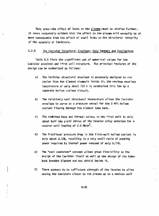
This area—the effect of leaks on the plasma—must be studied further. It seems reasonably evident that the effect on the plasma will normally be of more consequence than the effect of small leaks on the structural integrity of the assembly of Canisters.

5.2.9 The Canister Structural Envelope: Data Summary and Conclusions

Table 5.5 lists the significant set of numerical values for the Canister envelope and first wall structure. The principal features of the design can be summarized as follows:

a) The Canister structural envelope is purposely designed to run cooler than the blanket elements inside it; the maximum envelope temperature of only about 731 K is maintained this low by a separate helium coolant circuit.

b) The relatively cool structural temperature allows the Canister envelope to serve as a pressure vessel for the 5 MPa helium coolant flowing through the blanket tube bank.

c) The combined hoop and thermal stress in the first wall is only about half the yield stress of the Tenelon alloy selected for a

2 neutron wall loading of 2.0 HW/m .

d) The fractional pressure drop in the first-wall helium coolant is only about 0.102, resulting in a very small ratio of pumping power required to thermal power removed of only Q.17X.

e) The "cool container" concept allows great flexibility in the design of the Canister itself as well as the design of the tube-bank breeder blanket and hot shield inside it.

f) There appears to be sufficient strength of the Tenelon to allow moving the Canisters closer to the plasma up to a neutron wall

5-35

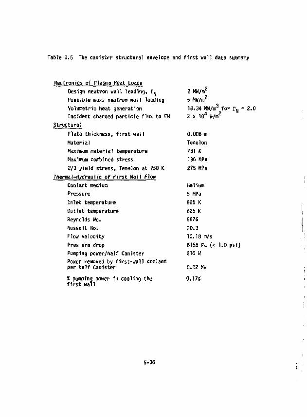
TabJe a.5 The canister structural envelope and first wall data summary

Neutromcs of Plasma Heat Loads Design neutron wall loading, F N 2 MW/m Possible max. neutron wall loading 5 MW/m Volumetric heat generation 18.34 MW/m3 for r N - 2.0 Incident charged particle flux to FH 2 x 10 W/m

Structural Plate thickness, first wall 0.006 m Material Tenelon Maximum material temperature 731 K Maximum combined stress 136 MPa 2/3 yield stress, Tenelon at 750 K 275 MPa

Thermal-Hydraulic of First Hall Flow Helium Coolant medium Helium

Pressure 5 MPa Inlet temperature 525 K Outlet temperature 625 K Reynolds No. 5676 Nusselt No. 20.3 Flow velocity 10.18 m/s Pres ure drop 5158 Pa (< 1.0 psiJ Pumping power/half Canister 210 W Power removed by first-wall coolant per half Canister 0.12 MW X pumping power in cooling the 0.17* first wall

5-36

loading of almost 5 MW/m . This has the possible advantage of decreasing the size and cost of the blanket and central cell magnet coils (at the expense of much shorter blanket lifetimes).

5-37

5.3 HEAT TRANSFER IN THE CANISTER VOLUME

Early calctlations in our first model of the Canister blanket indicated that it would be difficult to obtain a relatively large rise in the bulk coolant temperature (say 300 or 400 K) as the coolant flows across the lithium-oxide-filled tubes. The reason for the difficulty was the short travel distance, h, of the coolant since in this model of the Canister it was initially designed as a single pass heat exchanger as illustrated in Fig. 5.14. As a single pass system the thermal hydraulics were characterized by very low flow velocities, poor film coefficients of heat transfer, larger centerline temperatures in the lithium oxide than would be manageable, and higher tube temperatures than could be tolerated. Furthermore, in this model the first wall was not independently cooled.

Since the heat load and temperature range requirements are significantly different for the first wall than for the moderator volume, it was considered a better choice to provide separate cooling circuits. To cope with these anticipated design wsiderations of improving the thermal hydraulics and providing separate circuitry, a multiple pass heat exchanger was adopted as shown in Fig. 5.15. The illustration shows a two-pass heat exchanger. However, it is possible to use multiples of two passes with the same calcu-lational procedure. Because of the independent cooling circuit adopted for the first wall and the way this circuit is routed to deliver coolant down the center of the Canister and then up the sides, a half Canister serves as the calculational model for the thermal hydraulics and neutronics of the moderator/shield volume.

The calculational model for the blanket heat transfer may be described as a staggered tube, triangular pitch, crossflow heat exchanger. The dimen­sional parameters for the tubes and rods in this heat exchanger are shown in Fig. 5.16. All nomenclature used in the calculations and illustrations are listed in the appendices to this section.

5-38

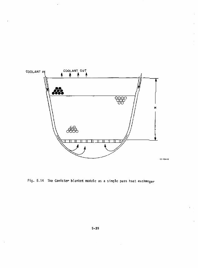
COOLANT IN COOLANT OUT T T t T

Fig. 5.14 The Canister blanket module as a single pass heat exchanger

5-39

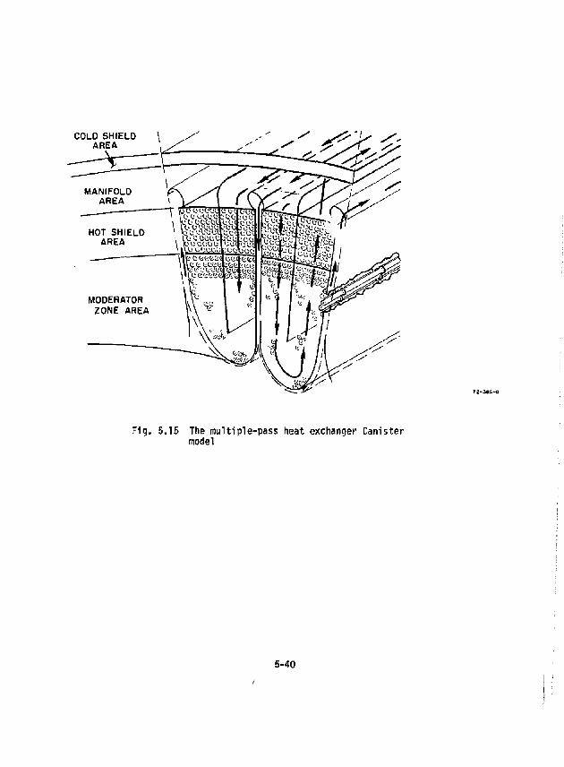
COLD SHIELD AREA

Fig, 5,15 The multiple-pass heat exchanger Canister model

5-40

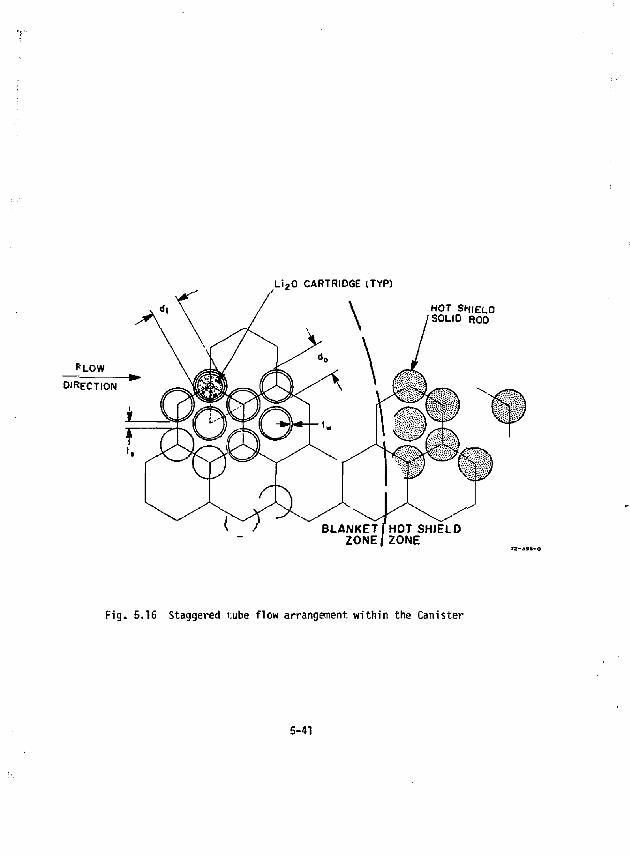
Li jO CARTRIDGE (TYP)

*LOW

DIRECTION

HOT SHIELD SOLID ROD

BLANKET fHOT SHIELD ZONE/ZONE

Fig . 5.16 Staggered tube f low arrangement w i th in the Canister

5-41

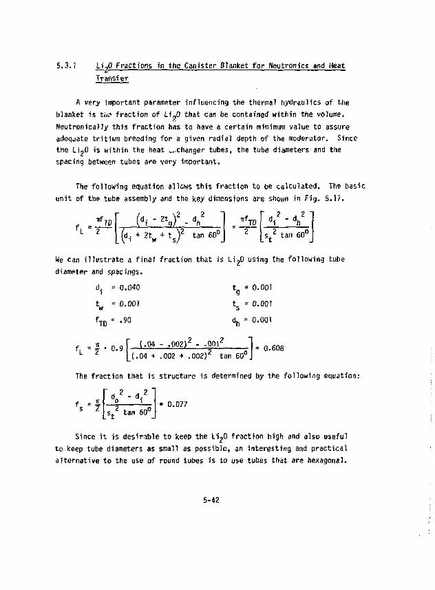
5.3.1 LigO Fractions in the Canister Blanket for Neutrom'cs and Heat Transfer

A very important parameter influencing the thermal hydraulics of the blanket is tha fraction of Li ?0 that can be contained within the volume, Neutronically this fraction has to have a certain minimum value to assure adequate tritium breeding for a given radial depth of the moderator. Since the LipO is within the heat changer tubes, the tube diameters and the spacing between tubes are very important.

The following equation allows this fraction to be calculated. The basic unit of the tube assembly and the key dimensions are shown in Fig. 5.1/,

\2 , 2 nf TD (-• - x - v (d. + 2t + t T tan V i w s/ 60u

iff. TO r H 2 A Z 1 di ~\ s t

2 tan 60°

We can illustrate a final fraction that is Li 20 using the following tube diameter and spacings.

d. = 0.040 t = 0.001 t = 0.001 w t s = 0.007 f T 0 = ,90 d h = 0.001

1 5 . o o r *• 04 - .002) 2 - .00 2 l - „ 2 U.M + .002 + .002) 2 tan 60°J 608

The fraction that is structure is determined by the following equation:

f. = d 2 - d . 2

o i s t

2 tan 60° 0.077

Since it is desirable to keep the LigO fraction high and also useful to keep tube diameters as small as possible, an interesting and practical alternative to the use of round tubes is to use tubes that are hexagonal.

5-42

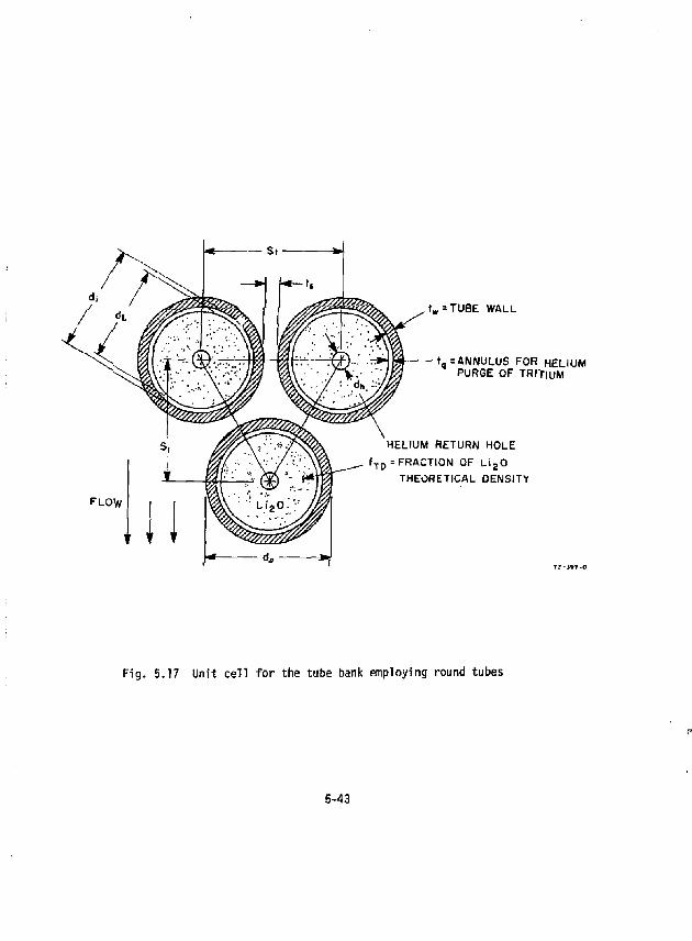
FLOW

1 iF-^<

«

t„ = TUBE WALL

t,=ANNULUS FOR HELIUM PURGE OF THIriuM

HELIUM RETURN HOLE f T p = FRACTION OF LigO

THEORETICAL DENSITY

Fig. 5.17 Unit cell for the tube bank employing round tubes

5-43

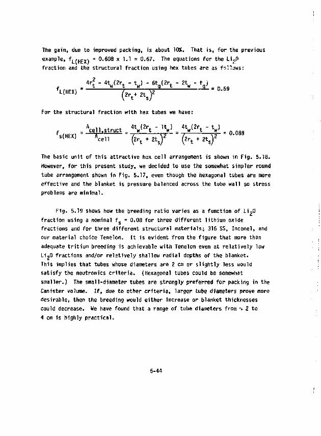
The gain, due to improved packing, is about 10%. That is, for the previous example, f|(nm * 0.608 x 1.1 = 0.67. The equations for the Li.,0 fraction and the structural fraction using hex tubes are as follows:

4 r t " 4 t w ( 2 r t " V _ 6 ta ( 2 rt • 2 tw " V f. , H m = —S *— j w i-I * S 3_ = 0.69

For the structural fraction with hex tubes we have:

f _ W s t r u c t V ^ ^ V V V fs(HEX) T ^ — - ( 2 P t + tts)Z~ " (2r t • 2 t s ) Z

= 0.088

The basic unit of this attractive hax cell arrangement is shown in Fig. 5.18. However, for this present study, we decided to use the somewhat simpler round tube arrangement shown in Fig. 5.17, even though the hexagonal tubes are more effective and the blanket is pressure balanced across the tube wall so stress problems are minimal.

Fig. 5.19 shows how the breeding ratio varies as a function of LigO fraction using a nominal f s = 0.08 for three different lithium oxide fractions and for three different structural materials; 316 SS, Inconel, and our material choice Tenelon. It is evident from the figure that more than adequate tritium breeding is achievable with Tenelon even at relatively low Li-0 fractions and/or relatively shallow radial depths of the blanket. This implies that tubes whose diameters are 2 cm or slightly less would satisfy the neutronics criteria. (Hexagonal tubes could be somewhat smaller.) The small-diameter tubes are strongly preferred for packing in the Canister volume. If, due to other criteria, larger tube diameters prove more desirable, then the breeding would either increase or blanket thicknesses could decrease. We have found that a range of tube diameters from *v 2 to 4 cm is highly practical.

5-44

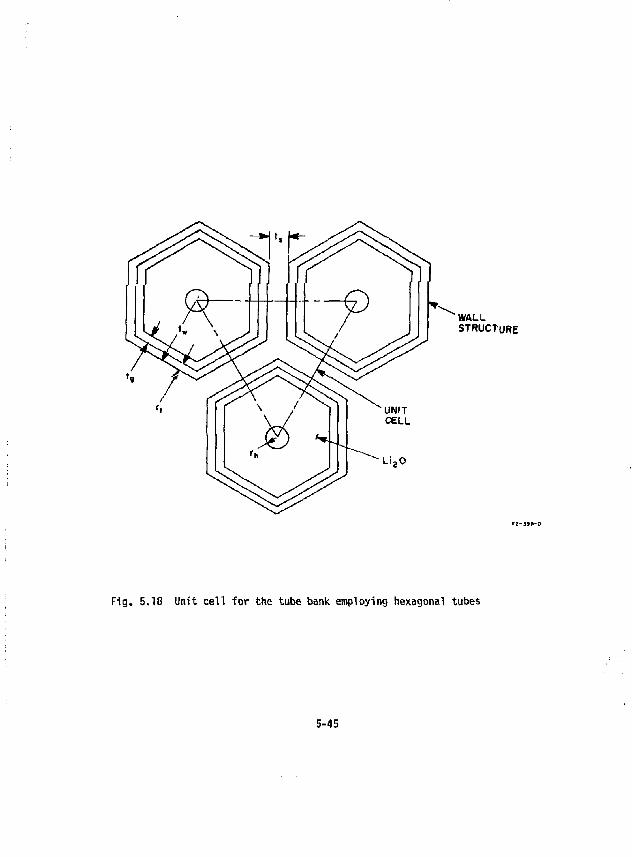
WALL STRUCTURE

F ig . 5.18 Unit ce l l f o r the tube bank employing hexagonal tubes

5-45

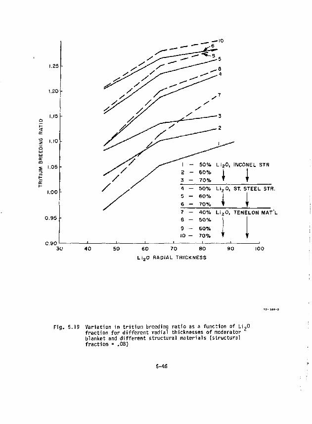
1.25

i.ao

<r en

3

ir

.15

1.10

1.05

1.00

0 .95

C .90 1

NCONEL STR

4 — 50% L i 2 0 , ST. STEEL STR. 5 - 60% 1 1 6 - 70% 1 1 7 - 40% L i 2 0 , TENELON MAT'L S - 50%

9 - 60% 10 - 70%

i i \

i

3U 4 0 50 6 0 7 0 8 0

L i 2 0 RADIAL THICKNESS

9 0 100

T2-199-0

Fig. 5.19 Variation in tritium breeding ratio as a function of Li 20 fraction for different radial thicknesses of moderator blanket and different structural materials (structural fraction = .08)

5-46

5.3.2 Tube Bundles in Crossflow

The heat transfer in flow over tubes in crossflow depends to a large extent on:

0 flow pattern 0 degree of turbulence 0 velocity of the coolant 0 size and arrangement of tubes 0 entrance effects 0 first row effects 0 numbers of rows and columns 0 side wall geometry

Furthermore, these influences are interrelated and consequently the flow pattern is too complicated to be treated purely analytically. Fortunately, there are experimental data available and empirical correlation equations have been developed that may be used to accomplish the heat transfer calcula­tions with good accuracy. It is interesting that these experiments indicate the transition from laminar to turbulent flow for staggered tubes in cross-flow is more gradual than in flow through a pipe, whereas for in-line tube bundles in crossflow the transition phenomena resemble those in pipe flow. This seems contrary to intuition since one would guess that the continuous velocity deflection in staggered tubes would more quickly induce turbulence. For our analysis this is informative but not directly relevant because the staggered tube arrangement is, in fact, a necessary selection over the in-line arrangement for minimizing neutron streaming. In either staggered or parallel tubes, the transition Reynold's number, important for our heat transfer calculations, begins at about 200, based on the velocity at the minimum flow araa specified by t of Pig. 5,17. The flow is fully turbulent at a Reynold's number = 6000.

For our engineering calculations, where the local internal heat genera­tion, w, in the Li ?0 and in the tube material falls off exponentially with

5-47

increasing radial distance from the first wall facing the plasma, we must l ; interested in both the local heat transfer coefficient, h„, and the average heat transfer coefficient h for the entire tube bundle. The local h„ and its accurate determination can be critical, particularly at the first row or so of tubes if this is where the energy deposition is the highest because the flow phenomena is singularly different than in the homogenized flow further into the array. For our particular model the energy deposition per unit volume falls off by about a factor of 20 from the first wall region to the back of the blanket (see the section on blanket neutronics). A built-in advantage of the flow model of our blanket heat exchanger is that flow enters at the hot shield at the back of the blanket where power density is least. Thereafter the flow across the continuously packed tubes is beyond the entrance effects. Local heat transfer coefficients are therefore not critical at the entrance region because heat fluxes are low and film temper­ature drops small. Recalling our first model single-pass heat exchanger, flow would flow across the tubes at the first wall where the power density is highest producing a much more severe condition of local heat transfer. This is another reason for preferring the multiple-pass system.

5.3.3 Heat Removal and Pressure Drop - Empirical Correlation Equations

The experimental data for flow across tube banks can be correlated by an equation of the form

{Wu) D = const(Re)1" (Pr) n

which can be recognized as being similar in form to correlations for flow in a tube or flow across a single tube. We have investigated the correlation equations of Kreith/ ' of Kays and London/ 2' of Grimison^, and of Eckert and Drake.^ ' They differ in detail, as for instance, how the velocity is determined or what reference length should be used in calculating the Reynold's number. However, the results of the four methods are comparable within -v 10%, which is quite good. Table 5.6 illustrates how well the methods compare.

5-48

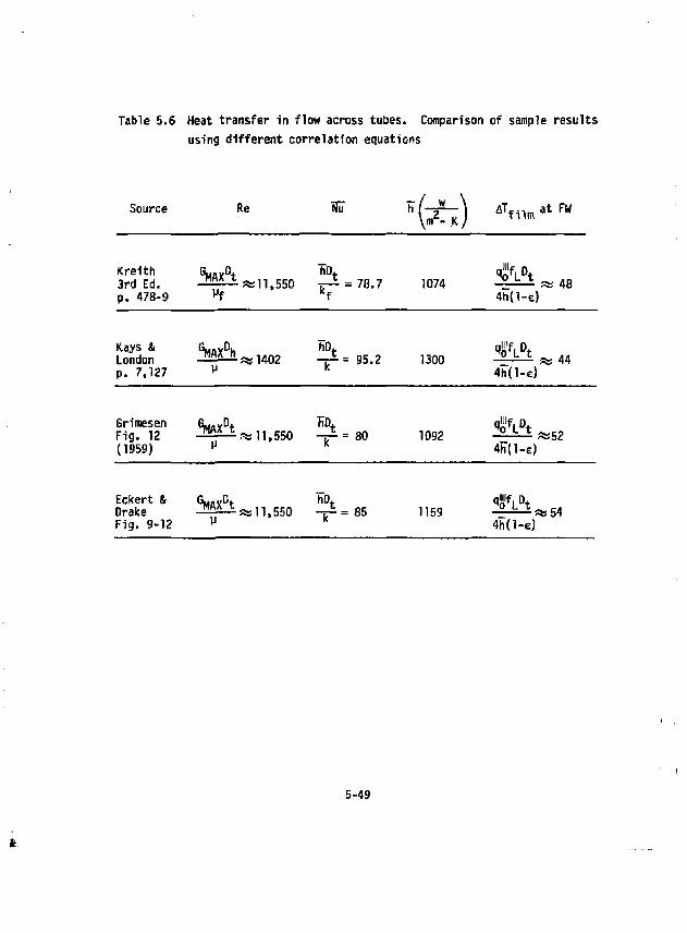
Table 5.6 Heat transfer in flow across tubes. Comparison of sample results using different correlation equations

Source Re Nu K ( ^ ) A T f i l * a t F W

Kreith GL..VD+ hD t q"'f, D t

3rd Ed. -££ * -= • as 11,550 T - ^ = 78.7 1074 _ » p . 478-9 vf K f 4h(l-e)

48

Kays & GuflvDu hDt qiilf. D London " " * n ^ 1402 - r ^ = 95.2 1300 ° L z as 44 p. 7,127 ^ K 4h(l-e)

Grimesen GMAA n£>* off. D t

Fig. 12 ™ * c ? a 11,550 - ^ = 8 0 1092 ° L c «s52 (1959) ^ K 4h(l-e)

Eckert & G^C,. hD. qW, 0f

Drake M f l * z as 11,550 - ^ = 8 5 1159 ° L ^ 5 4 Fig. 9-12 g K 4h(l-e)

5-49

In the data that follow the equations of Krei'th have been used. In the correlation equation for the average ff found in Kreith, the ve?ocity from which the Reynold's number is calculated is based on the minimum free area available for flow (t ). Since our tube arrangement is an equilateral triangle, the value of t. {the space between tubes shown in Fig. 5.17) is the same whether it is measured between tubes normal to the flow or on the diagonal.

The correlation for the Fanning friction factor, f , of Bergelin given in Fig. 5.20 was used for the tube bank pressure drop calculations (Kreith).

5.3.4 The Analytical Model Equations

Figure 5.21a shows the trace of the helium flow through the Canister as a two-pass heat exchanger. Figure 5.21b illustrates the local power density in the Canister for the numbered flow locations. It can be seen that the local power density repeats every two passes so that the general form of analysis presented here could be used for 2-n-pass systems. It was found early in our calculations that the two-pass heat exchanger was most appro­priate for this particular blanket design because of required tube diameters (2-4 cm) and the need to have a sufficient number of tube rows and columns so that the correlation equations for large tube banks would be valid. However, we also check film coefficients for the first tube row and check for edge effects for a tube that is in a first or last column.

The analysis deals first with the assembly of tubes followed by single tube analysis at appropriate locations.

The assumptions used in the analysis are as follows:

-r/r* 1) The power density has the form w = w e ' ror each pass,

where r is measured from the first wall region. 2) Negligible effect of turnarounds on temperature profiles. 3) Constant tube diameter of the staggered array.

5-50

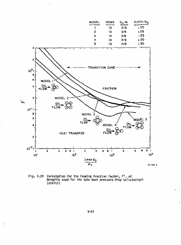
iflODEL ROWS Do IN. P l T C H / 0 0

i - • J » =T==fi=--^*-=

1 10 3/e 1.25 2 10 3 /8 1.25 3 14 3/8 1.25 A 10 3 /8 1.50 5 to 3 / 8 1.50

FLOW

|0 ' r 6

6 -

4

cQ- £ -

01L FLOW

HEAT TRANSFER FLOVT

l

I0 !

6 8 I

10 2

8 I

I 0 3

e i io 4

3 mat. D 0

Fig. 5.20 Correlation for the Faming fraction factor, f , of Bergelin used for the tube bank pressure drop calculat ion (Kreith)

5-51

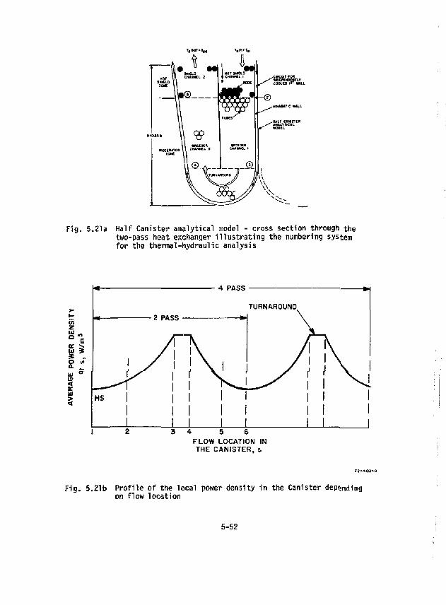
fHOMNKNTlV COOLCO (<> WALL

AOUUTIC WALL

HALF CIW1TEK ANAlflTKM. UOOCL

Fig. 5.21a Half Canister analytical model - cross section through the two-pass heat exchanger illustrating the numbering system for the thermal-hydraulic analysis

v> z HI o K Ul o a. LU a < id

3

FLOW LOCATION IN THE CANISTER,s

F ig . 5.21b P ro f i l e of the local power density i n the Canister depending on f low locat ion

5-52

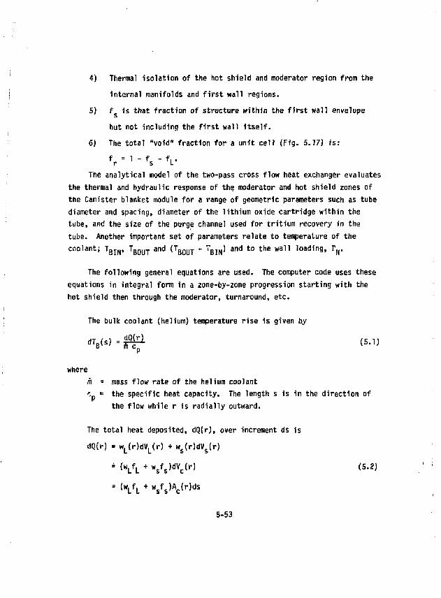
4) Thermal isolation of the hot shield and moderator region from the internal manifolds and first wall regions.

5) f is that fraction of structure within the first wall envelope but not including the first wall itself.

6) The total "void" fraction for a unit cell (Fig. 5.17) is: f = 1 - f - f, . r s L

The analytical model of the two-pass cross flow heat exchanger evaluates the thermal and hydraulic response of the moderator and hot shield zones of the Canister blanket module for a range of geometric parameters such as tube diameter and spacing, diameter of the lithium oxide cartridge within the tube, and the size of the purge channel used for tritium recovery in the tube. Another important set of parameters relate to temperature of the coolant; T B J N , T B 0 U T and ( T B 0 U T - " B j N ) and to the wall loading, r N.

The following general equations are used. The computer code uses these equations in integral form in a zone-by-zone progression starting with the hot shield then through the moderator, turnaround, etc.

The bulk coolant (helium) temperature rise is given by d T B ( s ) = £ 2 i l i (5.1,

where m = mass flow rate of the helium coolant c = the specific heat capacity. The length s is in the direction of

the flow while r is radially outward.

The total heat deposited, dQ(r), over increment ds is dQ(r) = w L(r)dV L(r) + w s(r)dv s(r)

= (w Lf L + w sf s,dV c(r) (5.2)

= £w Lf L + w sf s)A c(r)ds

5-53

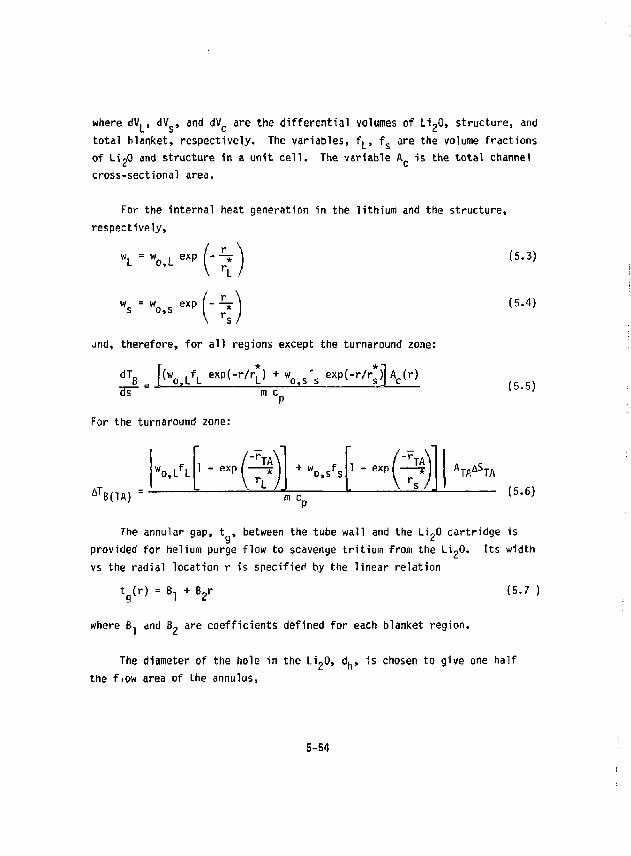
where dV. , dV , and dV c are the differential volumes of Li 20, structure, and total blanket, respectively. The variables, f L, f are the volume fractions of Li,0 and structure in a unit cell. The variable A is the total channel cross-sectional area.

For the internal heat generation in the lithium and the structure, respectively,

w L = w 0 j L exp I- — (5.3)

W s = wo,s e*P[-7 (5.4)

and, therefore, for all regions except the turnaround zone:

d T B _ K , L f L e x P < - ^ r L J + w o , s ' s exp(-r/r*j|Ac(r) Hs m c_ (5.5)

For the turnaround zone:

AT,

w o , L f L

B(TA)

1 - exp | 'TA 1

D,S S ' - -9* A T f t A S T A

m c„ (5.6)

The annular gap, t , between the tube wall and the Li^O cartridge is provided for helium purge flow to scavenge tritium from the Li 20. Its width vs the radial location r is specified by the linear relation

t g(r) = B 1 + B 2r (5.7 )

where B. and B~ are coefficients defined for each blanket region.

The diameter of the hole in the Li^O, d h, is chosen to give one half the fIOW area of the annulus,

5-54

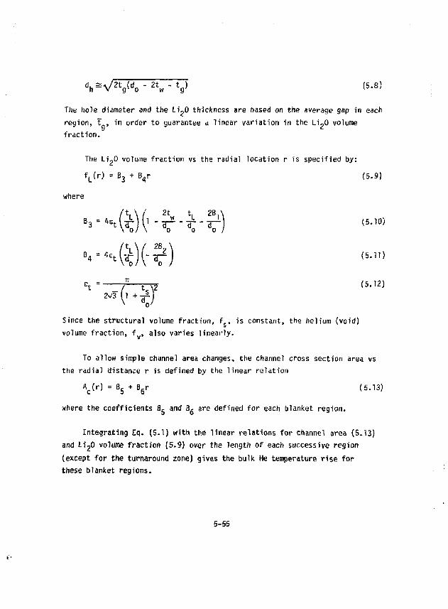
The hole diameter and the Li^O thickness are based on the average gap in each region, t-, in order to guarantee a linear variation in the Li,0 volume fraction.

The Li^O volume fraction vs the radial location r is specified by: f L(r) = B 3 + B 4r (5.9)

where

(5.12)

Since the structural volume fraction, f , is constant, the helium (void) volume fraction, f , also varies linearly.

To allow simple channel area changes, the channel cross section area vs the radial distance r is defined by the linear relation

A c(r) = B 5 + B 6r (5.13)

where the coefficients B g and B, are defined for each blanket region.

Integrating Eq. (5.1) with the linear relations for channel area (5.13) and Li'20 volume fraction (5.9) over the length of each successive region (except for the turnaround zone) gives the bulk He temperature rise for these blanket regions.

5-55

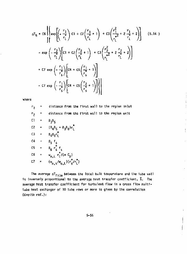
AT B = C6

where

'2 CI C2 C3 C4 C5 C6 a

exp - -j. + 2 - ^ + 2

- C7 exp

H")] (5.14 )

+ C7 exp - -y

^hK?" distance from the first wall to the region inlet distance from the first wall to the region exit

B3 85 (B 4B 5 • B 3B 6)r L

B 4B 6r* B 5 f S B6 rs ' s wo,L rV<m ty ( wo,s / wo,L» rs / rL>

The average AT f-, between the local bulk temperature and the tube wall is inversely proportional to the average heat transfer coefficient, h. The average heat transfer coefficient for turbulent flow in a cross flow multi-tube heat exchanger of 10 tube rows or more is given by the correlation iKreith ref.):

5-56

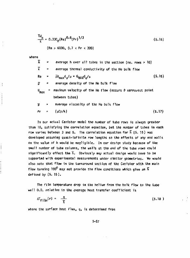
-|j£- 0.33C H{Re)°' 6{Pr) ? / 3 (5.15)

(Re > 6000, 0.7 < Pr < 300)

where h » average h over all tubes in the section (no. rows > 10) k" = average thermal conductivity of the He bulk flow R e ' P^axVn = G M A X d o ^ < 5 J 6 > p = average density of the He bulk flow U „ = maximum velocity of the He flow (occurs @ narrowest point 111 a A

between tubes) V = average viscosity of the He bulk flow Pr = (»iCp/k) (5.17) In our actual Canister model the number of tube rows is always greater

than 10, satisfying the correlation equation, but the number of tubes in each row varies between 3 and 6. The correlation equation for ¥ (5. 15) was developed assuming quasi-infinite row lengths so the effects of any end walls on the value of h would be negligible. In our design study because of the small number of tube columns, the walls at the end of the tube rows could significantly effect the h. Obviously any actual design would have to be supported with experimental measurements under similar geometries. We would also note that flow in the turnaround section of the Canister with the main flow turning 180 may not provide the flow conditions which give an h defined by (5. 15).

The film temperature drop in the helium from the bulk flow to the tube wall O.D. relative to the average heat transfer coefficient is

where the surface heat flux, q, is determined from

5-57

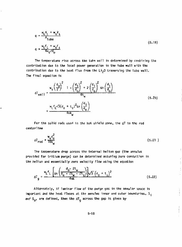
q =

q =

"lA * ws Vs tube

w L f L + w s f s (5.19)

The temperature rise across the tube wall is determined by combining the contribution due to the local power generation in the tube wall with the contribution due to the heat flux from the Li^O traversing the tube wall. The final equation is

Mr) i -AT,

+ 2 S.n wall 4k.

w L f L V 3 ( d Q + t/ln (Jjij + znnr —

(5.20)

For the solid rods used in the hot shield zone, the AT to the rod center!ine

AT rod $ (5.21 )

The temperature drop across the internal helium gap (the annulus provided for tritium purge) can be determined assuming pure conduction in the helium and essentially zero velocity flow using the equation

wiA *V

£.n / do- 2 tw V

y^K+ s) 2

(5.22)

Alternately, if laminar flow of the purge gas in the annular space is important and the heat fluxes at the annulus inner and outer boundaries, S^ and S Q, are defined, then the AT across the gap is given by

5-58

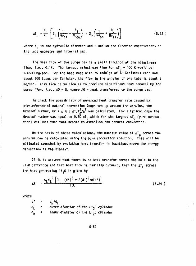
where d. is the hydraulic diameter and e and Nu are function coefficients of the tube geometry and internal gap.

The mass flow of the purge gas is a small fraction of the mainstream flow, i.e., 0.1%. The largest mainstream flow for ATg = 100 K would be ^ 6500 kg/sec. For the base case with 75 modules of 18 Canisters each and about 600 tubes per Canister, the flow in the annulus of one tube is about 8 mg/sec. This flow is so slow as to preclude significant heat removal by the purge flow, i.e., AQ « 0, where AQ = heat transferred to the purge gas.

To check the possibility of enhanced heat transfer rate caused by circumferential natural convection loops set up around the annulus, the Grashof number, Gr = p g 6 AT„t|l/u was calculated. For a typical case the Grashof number was equal to 0.30 AT which for the largest AT (pure conduc­tion) was less than that needed to establish the natural convection.

On the basis of these calculations, the maximum value of AT across the annulus can be calculated using the pure conduction solution. This will be mitigated somewhat by radiation heat transfer in locations where the energy deposition is the highes*.

If it is assumed that there is no heat transfer across the hole in the LipO cartridge and that heat flow is radially outward, then the AT. across the heat generating LipO is given by

w.d. 2 [l - ( d 1 ) 2 + 2(d')2tn(d')l i T L = - L L J T6T L T6L L t 5-* 4 >

where d' = d h/d L

d L = outer diameter of the LigO cylinder d. = inner diameter of the Li,0 cylinder

5-59

5.3.5 Illustration of a Design Case

Tables 5.?a through 5.7g contain sample output for a reference case where T B I N = 625 K and T B Q U T = 825 K.

5.3.6 The Influence of Structural Material Composition an Canister Design

The influence of structural materials and their composition on the neutronic performance of the Canister blanket was found to be a highly impor­tant, if not the most important, consideration in design. As can he inferred from Fig, 5.19, the use of materials such as Inconel drives the system to high lithium oxide fractions in order to get the tritium breeding greater than 1.0. Structurally, because the lithium oxide is contained within the tubes, the tube diameters must increase. With Inconel, tube diameters must be approximately 4 cm to achieve proper tritium breeding. With Urge tube diameters the inner temperature of the lithium oxide at tha purge hole surface increases a.nd this sets a constraint on the design. Inconel also has high internal heat generation due to high neutron/gamma capture, the net result of which is to lower the blanket energy multiplication, M. Topolog­i c a l , larger tube diameters also make it more difficult to load a given Canister uniformally with tubes. The number of tube columns and the number of tube rows simply cannot be an integer multiple of a dimension as large as 4 cm.

The non-nickel alloys, such as Tenelon or 2.25 Cr-1 Mo or 316 SS, allow substantially lower lithium oxide fractions and hence smaller tube diameters (if temperature permits). Tube diameters of 2 cm, producing 0.4 lithium oxide fraction, intrinsically yield breeding ratios greater than 7,10 for our Tenelon design case where the moderator radial thickness is 0.65 m. Further­more, for Tenelon, the blanket multiplication factor is 1.24 as compared with the Inconel case where M was 1.16, a gain of aJmost 7% or, in terms of power, an additional 224 MW. If the 0.4 lithium oxide fraction is retained and the blanket radial thickness decreased to 0.45 m, the blanket multiplication increases to 1.26, yielding approximately 280 MW more than would be obtain-

5-60

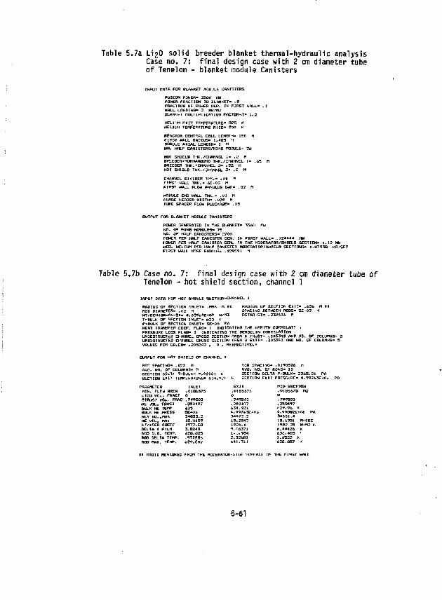
Table 5,7a LigO solid Case no, 7; of Tenelon •

breeder blanket thermal-hydraulic analysis final design case with 2 cm diameter tube blanket module Canisters

INPUT DATA FOR BLANKET MODULE CANISTERS FUSION POWER- 3500 MM PdMER FRACTION TD BLANKET- .6 FRACTION OF PDweft DEP. IN FIRST WALL-MALL LOADING- 2 nw/M2 BLANKET MULTIPLICATION FACTOR-IT- 1.2

REACTOR CENTRAL CELL LENGTH- ISO ri fIRBT WALL RADrUS- 1.463 II MODULE AXIAL LENGTH- 2 H NO. HALF CANISTERS/RING MQDULE= 36 HOT SHIELD THK./CHANNEL 1- .2 M BREEDER'TURNAROUND THK./CHANNEL I- . PftEEDER THK.fCHANNEL 2- .52 M HOT SHIELD THK./CHANNEL 2- .2 H CHANNEL DIVIDER THK.- .01 ft FIRST WALL THK.- AE-P7 M FIRST MAIL FLOW AFWULUS GAP- .02 PI MODULE EMp UAU, TW,- -01 M PUAQE HEADER MTDTHB .O?? M TLIPE SPACER FLQw K.OCKWJE- .05

OUTPUT FOfi BLANKET MODULE CANISTERS POWER GENERATED IN THE BLANKET* 134 Ci KU NO. OF RINB MODULES- 75 NO. OF HALF CANISTERS- 270O POWER PER HALF CANISTER GEN. IN FIRST MALL- .124444 MM rawen PER HALF CANISTER GEN. TN THE MODERATOR/SHIELD SECTION- 1.12 MH HEO. HELIUM PER HALF CANISTER HODERAT0ft/SHIELD SECTIONS- 1.0793B KG/SEC FIRST HAUL NDSE RADIUS- .129591 H

Table 5,7b Case no. Tenelon

7: final design case with 2 cm diameter tube of • hot shield section, channel 1

INPUT DATA FOR HOT SHIELD SECTION-CHANNEL 1

RADIUS OF SECTION E U T - . 6 3 6 SPACING BETWEEN RODS- 2 E - 0 3 RSTAR-ST- .2-30636 PI

M tt RADIUS OF SECTION INLET- ,856 rti* ROD DIAMETER- ,03 (1 HT/GEMtiR-O-ST- 4,.63969E+07 M/H3 T-BULK OF SECTION INLET- 623 K P-BOLfc OF SECTION INLET- 5E+06 PA HEAT TRANSFER COEF. FLAG- 1 INOICATINO THE KREITH CORRELAT' * PRESSURE LOSS FLAG- 1 INDICATING THE BERGE1IN CORRELATION UNOBSTRUCTED CHANNEL CROSS SECTION AREA 3 INLET- .205343 AND NO. OF COLUMNS- 3 UNOBSTRUCTED CHANNEL CROSS SECTION AREA 3 EXIT- .205343 AND NO. DF COLUMNS- S VALUES FOR CA.CB- .205343 . O . RESPECTIVELY

OUTPUT FOR HOT 5HIELD OF CHANNEL I ROD SPACING- .027 H AVG* MO, OF COLUMNS- 5 SECTIDN DELI* 1-BULY.- 9.92051 K SECTION EXP TEMPERATURE" 634.921

ROW SPACING- .0)70-326 H AVB. NO. OF ROUS- 1& SECTIDN DELTA P-BULK- 2363.Bt PA SECTION EIIT PRESSURE- 4r997bZE+0L

PARAMETER INLET EXIT MID SECTION n i N . FLPU AREA . 0 1 B 6 6 7 3 .0 IB6!»75 . 0 3 0 6 6 7 5 HZ L I 2 D VOL. FRACT 0 0 0 STRUT! f VOL. FflAC . 7 4 9 5 0 3 . 7 4 9 5 0 3 . 7 4 9 3 0 J HE JOL. FBACT . 2 3 0 4 9 7 . 2 5 0 4 9 7 -Z30497 BULK HE T E W 623 6 3 1 . 9 2 1 *2«* .94 K BULK HE PRESS 3 E * 0 6 4.<?<?7fr!£+C'A 4 . q v 0 g 3 E * o i , pa REV MO.,MAT 34H33 .2 3 4 4 7 2 . 2 3 4 6 6 1 , 4 HE VEL, MAX 1 3 . 0 1 3 9 I S . 2 3 4 7 13 .1391 H/SEC H f / x F E A COCFF 1977.BH 1 9 D 6 . 6 1982 .23 HVH2 K DELTA f fILH 3. B24B 9 . i1&37l 6 . 4 4 4 7 6 K ROD O.D. TEMP. 6 2 0 , 6 2 5 t- J.9BA 6 3 6 . 4 0 3 ' ROD bELTA TEMP, -9773B6 2 . 3 2 6 9 1 1 . 6 3 2 2 K ROD MAX. TEMP. 6 2 9 . 8 0 2 6 4 6 . 3 1 1 6 3 0 . 0 3 7 K

• • RADI I MEASURED FROM THE MODERATQR-Sll/E SURFACE OF THE FIRST WALL

5-61

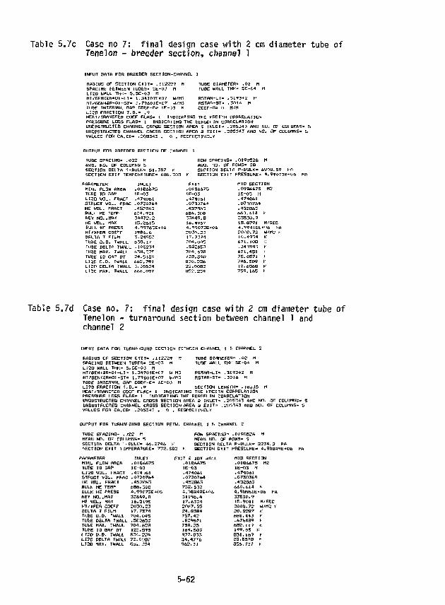
Table 5.7c Case no 7: f inal design case with 2 cm diameter tube of Tenelon - breeder section* channel 1

TUBE DJAM£TER« .OZ M TU&C WALL THK- 5E-04

INPUT DATA FOR BREEDER SECTION-CHANNEL 1

RADIUS OF SECTION EKIT" .1122:29 PI SPACING &ETHEEN TUDES- 2E-03 M LI213 WALL THK- 5.3E-03 H H T / G E N ( 5 ) R » 0 I - L 1 - 1 . 3 4 7 0 I E + 0 7 W^t f j H J V G E N * a R * O J - 5 T - J . 7 9 6 0 1 E * D 7 W/M3 TU&E INTERNAL GAP C O E F - F o 1 E - 0 3 H L I 2 0 FRACTION T . D . - . 9 HEf tT /TRANEFER COEF F L A f l " 1 I N D I C A T I N G THE K R E I T H CORRELATION PRESSURE LOSS F L A B - I I N D I C A T I N G THE BERQEl I N CORRELATION UNOBSTRUCTED CHANNEL CROSS SECTION AREA S I N L E T - , 2 0 5 3 4 ? AND NO. OF COLUMNS-UNOBSTRUCTED, CHANNEL CROSS GECT ION AREA 3 E X I T - . Z 0 5 ! M 3 AND N O . OF COLUMNS" ! VALUES FOR C A . C B « • 2 0 5 3 4 3 . 0 . RESPECTIVELY

RBTAR-LI-RSTAR-ST-COEF-G= 0

.319342

.3016 M

OUTPUT FOR &REEDER SECTION OF CHANNEL 1

IUBE SPACING- .022 M AVG. NO. OF COLUMNS S SECTION DELTA T - B U L K " 5 I . 3 B 7 r. S E C T I O N E X I T TEMPERATURE- 6 8 6 . 3 0

PARAMETER n i N . FLOW fitter* TUBE I P CAP L I 2 0 V O L , FRACT STf iUCT V D L . FRAG HE V D L . FRACT BULK HE TEMP KEY N O . * M A * HE V E L , M&x BULK H r PRESS HTi-XFER CQEFF DELTA T F I L M 1U&E fl.O. TWALL TUBE DELTA THALL TU&E MAX. TUALL TU&E I D GAP DT H 3 D Q . D . TWALL L I 2 0 DELTA TWALL L I S n MAX* TWALL

RDM S P A C I N G * , 0 1 9 Q 3 2 4 M AVG. NO. OF ROMS" 2B SECTION! DELTA P-PULK- 6908.39 PA SECTION ES1T PRES5URE- 4.99073E+06

INLET EKTT H I D S E C T I O N . 0 1 6 6 6 7 5 . 0 1 9 6 6 7 5 . 0 1 8 6 6 7 5 T12 I E - 0 3 I E - 0 3 I E - 0 3 t i . 4 7 4 0 6 1 .A74< j£ h | . 4 7 4 0 4 1 . 0 7 3 0 7 4 4 . 0 7 3 ( 3 7 6 4 . 0 7 3 0 7 4 4 . 4 5 2 B 6 3 . 4 5 2 B 6 3 . 4 5 I B 6 3 6 3 4 , 9 2 1 6 B 6 . 3 0 S 6 6 0 , 6 1 4 y 3 4 1 7 2 , 2 3 2 6 4 9 , G 3 3 5 3 0 . 9 1 5 . 2 6 1 5 1 6 . 1 7 6 7 1 5 . 8 7 9 1 He-SEC 4 . 9 9 7 6 3 E * 0 6 4 . *3 *?073E*06 4 . 9 P 4 1 S E - f ' 6 P< 1 9 0 6 . 6 r o s r t . 2 3 r O t f f l . 7 2 W/M? J 3 . 2 4 9 5 3 1 7 . 7 ^ 7 4 1 0 . 4 9 3 4 K 6 3 0 , 1 7 7 0 4 , 0 4 5 6 7 1 . | 0 G k . 1 0 5 2 3 4 . 5 3 2 6 5 3 . 3 4 1 9 4 3 Y 6 3 0 , 2 7 5 7 0 4 . 6 2 A 6 7 1 , 4 5 1 \ 2 4 . 5 r 3 ? f 2 5 . 3 ? S 7 5 , 0 3 7 1 > 6 6 2 * 7 9 1 B3t>. 2 2 6 7 4 6 . 5 0 9 1' 3 . 3 0 5 3 1 2 2 . 0 0 B 2 1 2 . 6 5 6 8 K 6 6 6 , 0 9 7 B 5 2 . 2 3 4 7 5 9 . 1 6 5 t

Table 5.7d Case no. Tenelon channel

7: final design case with 2 cm diameter tube of - turnaround section between channel 1 and

INPUT DATA FOR TURNAROUND S E C T I O N K T W E E N CHANNEL I !< CHANNEL 2

RADIUS OF S E C T I O N E K T T - . 1 1 2 2 2 9 Ft SPACING BETWEEN T U P E S " 2 E - 0 3 M L I 2 D WALL T H K - S , 5 E ~ Q 2 M H T / G E N O R - O I - L l - 1 . 3 4 7 0 1 E + 0 7 W H3 H T / G E N O R * 0 > - B T » 1 . 7 9 6 0 1 E + 0 7 h / f i 3 TU&E INTEftFWL C V C D E F - C " J E - O i M L I 5 D FRACTION T . D . - . 9 HEAT/TRANSFER CQEF F L A G - 1 I N D I C A T I N G THE K R E I T H CORRELATION PRESSURE LOS.P F L A G - 1 I N D I C A T I N G THE BERGEL IN CORRELATION UNOBSTRUCTED CHAN'JEL CROSS S E C T I O N AREA 5 INVFTT-. , 2 0 5 3 * 3 AND NO. OF COLUMNS^ UNOBSTRUCTED CHANNEL CROSS S E C T I O N AREA A E X I T - . 2 0 5 3 4 3 AND NO. OF COLUMNS* : VALUES FOR C A . C B - , 2 0 3 3 4 3 • 0 . RESPECTIVELY

TUBE DlAnETER" . 0 2 TU&E WALL TH> 5 E - 0 *

R S T A R - L I * R S T A R - S T *

SECTION L E N G T H - • 1 0 3 3 5

OUTPUT FGR TURNAROUND S E C T I U N RETW. CHANNEL 1 h CHANNEL 2

TUBE S P A C I N G - . J22 Ft H£AN NQ, OF Cp l UWNB- E SECTION DELTA ' -BULK«> 4 6 . 2 7 4 6 SECTION E K I T 1=MPERATURE- 7 3 2 , 1

PAfVWElER H i r ( . FLOW AREA ILf&E I D SAP L I 2 0 V O L . FRACT STRUCT V O L . FRAC HE UDL. FRAHT BULK ME TEMP &UL.K HE PRESS KEY NO. .MAX HE V E L , MA I HT.-KFEfi CDEFF DELTA T F I L n TJJBE O . D . TWALL TUBE 0 £ L T f l THALL TUbE HAX. 7UALL TUBE I D GAP PT LIZO (?•!>• THALL L I 2 D DELTA TwALL L T J O MAX- THALL

ROW 5PAC»WG= . O J 9 0 5 2 A ft MEAN NO. OF ROWS* 9 SECTION DELTA P-BULK~ 2234.2 PA SECT1DN EXIT PRESSURE- 4. <JaB49E+06

IWLET cxn a IBT WALL M I D SECTION . 0 1 ^ 6 6 7 5 . 0 1 ^ 6 6 7 5 . 0 1 0 6 4 7 5 M2 I E - 0 3 1 E - 0 3 1 E - 0 3 f t . 4 7 4 ,6,1 . 4 7 4 0 4 1 . 4 7 4 0 6 1 . 0 7 i 0 7 4 4 . 0 7 3 0 7 6 4 . 0 7 S 0 7 6 4 . 4 5 2 ( 7 6 3 . 4 3 2 0 6 3 . 4 5 2 B 6 3 6 B 6 , 3 0 B 7 3 2 . 5 6 2 6 6 0 , 6 1 4 K 4 . 9 9 0 7 3 E * 0 6 4.7as49E-«->' i6 4 . 9 B 9 6 1 E * C I 4 PA 3 2 6 4 9 , 0 3 1 1 9 6 , 4 3 3 5 3 0 , 9 1 6 . 3 1 9 5 1 7 . 4 3 3 4 I E . 9 0 1 1 M/SEC 2 0 3 0 . 2 3 2 0 6 7 . 5 5 2ooa.72 w/na t-t 7 - 7 3 7 4 Z 4 - 9 5 f l 4 2 0 . 0 2 B 7 t: 7 0 4 . 0 4 5 7 5 7 . 4 2 6 0 1 . 4 4 3 h' . 5 B 2 6 5 ; . B 2 9 5 7 1 . 6 7 & 4 B 9 » 7 0 4 . 6 2 G 7 5 H . 2 5 6 B 2 . 1 1 9 t. 1 2 3 . 5 9 9 1 6 9 , 5 0 3 1 4 9 . 0 5 >:

33*. r r * 9 J 7 . 0 3 3 0 3 1 . 1 6 ? r 2 2 . 0 0 B ? 3 4 . 4 7 7 6 2 5 , 5 3 7 0 ^ G a l . :34 9 4 2 . 3 1 0 5 6 . 7 ^ 7 t:

5-62

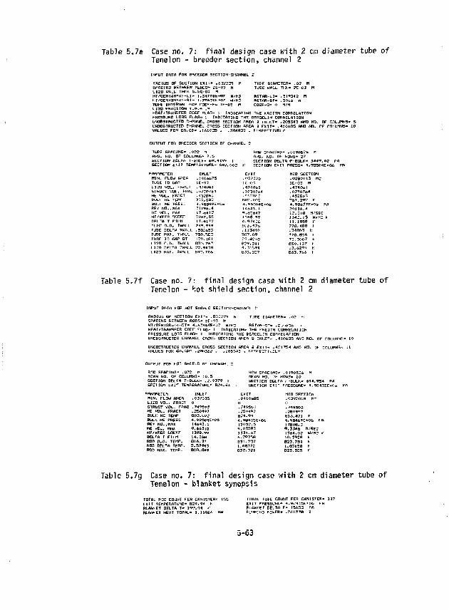
Table 5«7e Case no. 7: f inal design case with 2 cm diameter tube of Tenelon - breeder section, channel 2 INPUT DATA FDR BREEDER SECTION-CHANNEL 2

RADIUS OF SECTION E I I T * . 6 3 2 2 2 9 M SPACING BETWEEN T L l K S - ZE-03 n L I Z O UflLL THK= 5 . 5 E - 0 I M HT/'GEJUiR=0)-LI- ].34701E+07 N/MJ HT/GENOP-Ol-Sf- l.79AOI£*07 u/ni TUGE INTERNAL GAP CrjEF-F= 1E-OJ M UI30 FRACTION T.O.- .<» HEAT/TRANSFER COEF Pi.AG- i INDICATING THE r.RErTH CORRELATION PRESSURE LOSS FLAG- 1 INDICATING THE EERGELlN CORRELATION UNOBSTRUCTED CHANNEL CROSS SECTION AREA i INLET- .303343 AND NO. OF COLUMNS- 5 UNOBSTRUCTED CHANNEL CROSS SECTION AREA 9 CHIT' -4I06B3 AND MO. OF COLUMNS- 10 VALUES FOR CA.CB* .161025 . .394809 , F-.SPECTIVELV

RSTf lR -L l= . 3 1 9 3 4 2 RSTAR-9T- . 3016 r C O E F - G B O M/M

OUTPUT FOR BREEDER SECTION OF CHANNEL :

TUfE SPACING- . W 2 n AVG. NO. OF COLUMNS* 7,5 SECTION DELTA T-Bill-.- 69. 4Jt9? 1 SECTION E*JT TEMPERATURE- B02.O02 K

FtOW SPACING" .0190516 M AVE. NO. OF ROWS- 27 SECTION DELTA P-BULK- 3 4 4 9 . 4 S fit SECTION EXIT PflESS- 4 .?B5C" lE f06

PARAMETER tttLBT EXIT MID SECTION M I N . FLO.J AREA .£•104475 . 0 3 7 3 3 5 . 0 2 6 0 0 1 3 m TUBE ID DAP 1E-07 IE -07 1E-03 M L I 2 0 VOL, FRACf .47*Oi>l .4 7 4 P M . 4 7 4 0 o l STRUCT VOL. F^AC .<• 73P744 . 0730764 . 0730764 H i VOL. FHACT , 4 5 ^ 0 6 ^ . i L r a & ; . 4 5 2 3 * 3 &L*-V ME T p V 1 7 T : r s e r E f c . c o ; 7&7.-29Z V BU_I ME Pf.E&r •).SB049E»O6 *.<»B504E"?ft 4 . 9 S 6 7 7 E - 2 ! , 1 REv IMO. , ClAX " I I S * , , 4 1 4 * 4 3 . i 2 r t l 3A. 4 HE VEL, MAX 17.64 12 9 . i 3 t i 4 7 i r . ^ i d M/s£c HT/<FER CCF.FF 2i«A7. S3 1 3 9 3 , 9 9 i £ 4 ± . j 9 M/nz DELTA T F ILM 17 .4172 fl.97436 11 .1959 I" TUI-E O . D . TWALL 7-19.799 B O i . 9 7 6 7 7 6 , 4 0 0 1 TUBE DELTA TUALL . 5 0 ^ 6 3 3 .11340V .34BO? t: TUT€ MAH. TWALL 7S0 .5B2 8 0 7 . 0 9 7 7 9 . B 3 6 t TUBE ID GAP DT 120. 1B1 2 2 . 4 1 0 8 7 1 . 3 0 0 7 * 1.120 O.D. TWALL B70.7&3 9 2 9 . 3 1 1 0 3 0 . 1 3 7 f L I 2 0 DELTA 7WALL 2 2 . 9 4 3 0 4 .31S9A 13 .A299 K L I 2 0 MA If. 1WALL B93. 706 B33 .B27 BA3.76(> ^

Table 5.7f Case no. 7: f inal design case with 2 cm diameter tube of Tenelon - hot shield section, channel 2

INPUT DATA FOR HOT S K I E L D SECTICN'-CHfitW^L Z:

RADIUS OF 5ECTI0N EX IT - . 0 ^ 2 1 7 9 h TUBE DIAnETER- . 0 2 *l SPACING BETWEEN RODS-- 2E-03 H HT/GEN13R=0)~ST= 4 . 6 3 9 6 9 E - 0 7 UVH3 RSTAR-STw . 2 U i 6 3 6 i HEAT/TRANSFER GOEF FLAG* 1 INDICATING THE Kf iEITH CORRELATION PRESSURE LOSS FLAG- 1 INDICATING THE BERGELIN CORRELATION UNOBSTRUCTED CHANNEL CRflSE. SECTION AHEA 3 INLET=f .4104SS AND MO. OF COLUTtNS- 10

.151 34 AND NO. DF COLUMNS'*

OUTPUT FOR HOT SHIELD or CHANNEL r RDD SPACING" .022 H MEAN NO. OF COLUMNS- 10.5 SECTION DELTA T-&UJ.K- ^J. 9379 I SECTION EXIT TEMPERATURE" B24.94 i

ROW SPACING- .0I90S2& M MEAig HO. OP ROUS' 10 SECTtOfl DELTA f -BULK* 6 9 4 . 7S« PA SECTION EXIT PRESSURE- 4.9B433E*0i

PARAMETER INLET EXIT MED SECTIOM M[N. FLOW AREA . 0 3 7 3 3 5 .0410bSS . 0 3 9 2 0 1 8 M I L1Z0 VOL. FRACT 0 ( I 0 STRUCT VOL. FfiAC : .74J9-03 , 749SO?- . 7 4 9 5 0 3 HE VOL. FRACT .250497 . 250497 . 2 5 ^ 4 9 7 BULK HE TEMP Q02. V02 H 2 4 . 9 4 B l i . 4 7 1 r BULK ME PRESS 4 .9 f f 3p iE *P f r 4 . ' *a4 3 5 E - 0 b 4,SB46SE*0fc I'A A E V f i o . , n f l * I 4 & 4 3 , 1 13032 .3 t 7B0S.3 he VEL, HAK 9 , 4 6 3 i g 9 . 0 3 3 9 3 9 . 3 J 4 6 rl/SEC HTVxFEA tOEPf I 3 9 8 . V 9 1 3 3 1 . 6 7 1 3 6 4 . o r W / n r K DELTA T F ILM lA.?h& fc.3975B i o . 2 B 2 a • ROD P.O. TEMP-. Q16. 27 B 3 1 . 2 3 7 B 2 3 . 7 5 4 k ftOD DELTA TEMP. 7.37943 1.0B371' 1 .031S9 I-' ROD MAK. TEMP. B I B . 6 4 9 0 3 2 . 3 2 1 B23.SB5 k

Table 5«7g Case no, 7: f inal design case with 2 en diameter tube of Tenelon - blanket synopsis

TQIAL ROD COLWT FER CANISTER" E U T TEMPERATURE- H 2 4 . 9 * t-BLAr^tET DELTA T - 1 9 9 . 9 4 ¥ BLAfJ> ET HEAT TOTAL- 1.1196A *

1UIAL l u t e COUNT FER CANISTER-EXIT PRESSURE- 4.93432E»C*> PA P L A N I E T DELTA P . 13653 PA PUT*»lH3 FEWER- . 31137B Z

5-63

able with the Inconel. The provision in this case would be that the tube diameters would have to be 3 cm. As can be seen from the above examples, there are many combinations of tube diameters, lithium oxide fraction, breeder radial thickness, etc., that will produce a good blanket assembly. What follows are some of the preliminary results of the parametric studies.

5.3.7 Parameter Study Preliminary Results - Minimum and Maximum Lithium Oxide Temperatures

Figure 5.22 illustrates the minimum lithium oxide temperature as a function of tube diameter for four different helium coolant flow rates pro­ducing four different levels of helium bulk temperature rise from inlet to outlet of the blanket. In this figure it can be seen that there is essen­tially zero sensitivity of the oxide minimum temperature due to tube diameter, which is as one would e/pect since the minimum temperatures occur at the flow entry into the blanket where the energy deposition is the least. The strong influence is the bulk temperature rise which determines the flow velocities and hence film temperature coefficients of heat transfer. At the reference case where the bulk temperature rise is 200 K, the lithium oxide minimum temperature is estimated to be approximately 770 K, well above the minimum temperature required to maintain a tritium inventory less than 1 kilogram (see Section 5.6).

Figure 5.23 shows the more important maximum lithium oxide temperature as a function of tube diameter and bulk helium temperatu.-e rise. In this case the maximum temperature occurs at the inner surface of the lithium oxide for the cartridge located at the point of maximum energy deposition, i.e., near the exit of the turnaround in the blanket near the first wall. Here the bulk temperature rise has little effect but the dominant influence is the tube diameter. This dominance of the diameter is because the energy deposi­tion is increasing in proportion to the diameter squared and at the same time the path length for energy removal is increasing with the diameter so the effect is roughly a cubic. Of concern here is to stay well below the teroper-

5-64

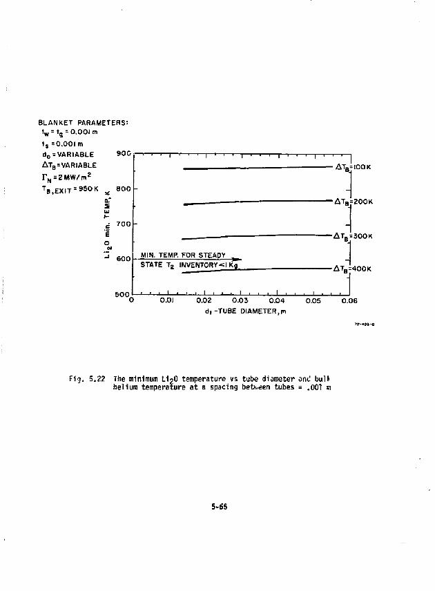
BLANKET PARAMETERS: t w = tg - 0.001 m t s =0.001 m d 0 = VARIABLE 900 AT B = VARIABLE r N =2MW/m z

TB,EXIT = 950K

TEM

P.K

800

i o

700

€00

5 0 0

MIN, TEMP. FOR STEADY STATE T 2 INVENTORY-el Kg

JL_i_ _L

— AT B=IOOK

0.01 0.02 0.03 0.04 d, -TUBE DIAMETER,m

0.05

•AT B=200K

•AT B=300K

•ATB=400K

J l__l L. 0.06

Fig. 5.22 The minimum LioO temperature vs tube diameter and bu1fr helium temperature at a spacing betv.den tubes = .001 m

5-65

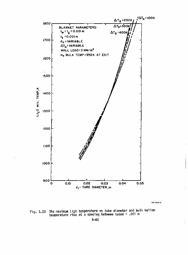
A T B =200K J

900'

1 ( BLANKET PARAMETERS t w = t„ = 0.001 m

d 0 = VARIABLE AT e = VARIABLE WALL L0A0= 2 MW/m H. BULK TEMP=950K AT EXIT

AT B=300K'

AT B = 4 0 0 K | J I

,'ATB = lO0K

0.01 0.02 0,03 d t-TUBE DIAMETER,m

0.04 0.05

23 The maximum L12O temperature vs tube diameter and bulk helium temperature rise at a spacing between tubes = .001 m

5-66

ature at which the lithium oxide melts (1970 K ) . Initially, -it was felt that there was a critical sintering temperature but a new method of fabricating the lithium oxide may eliminate that problem. This sintering and the method for LijO fabrication are discussed in Section 5.4 on tritium recovery. Nevertheless, it is advantageous to use the smaller diameter tubes. The actual temperature rise across the lithium oxide as a function of tube diameter is shown in Fig, 5,24.

Figure 5.25 illustrates lithium oxide maximum temperature as a function of neutron wall loading for a family of tube diameters. Clearly the smaller tube diameters are superior and if the higher wall loadings are to be achieved, then tube diameters of about 2 cm or 2.5 cm are to be strongly preferred. We do not know definitively how near to the melting point it is possible to operate the Li^O ijut a safe value may be approximately 0.80 or about 1575 K, This may be unduly optimistic, forcing the design to smaller diameter tubes.

5.3.8 Parametric Study - Maximum Tube Temperatures

Figure 5.26 shows maximum tube temperatures as a function of wall loadinp for selected tube diameters. For this parametric study, the wall loading was increased by moving the Canisters closer to the central-cell plasma while keeping the total fusion power constant. In addition, the radius of the first wall of the Canisters was kept constant, and the number of Canisters per ring module was reduced appropriately as the Canisters were moved closer to the plasma. The helium inlet and exit bulk temperatures were also held fixed at 625 K and 825 K, respectively.

The maximum tube-wall temperatures were found to occur close to the exit of the second breeder zone (point 5 on Fig. 5.21). As can be seen from the results in Fig. 5.26, this temperature, T 5, does not vary appreciably for a factor of 2.5 change in the wall loading or a factor of 2 change in the tube diameter. This result can be explained as follows. The total helium flow rate to each ring module did not change for all of the above calculations,

5-67

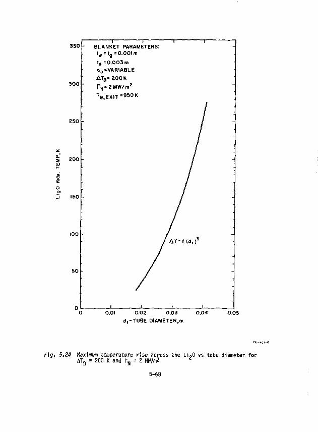
350

300

250

1 —T~ - BLANKET PARAMETERS:

i w = tg = 0.001 m 1t =0.003 in t i 0 = VARIABLE AT B =200K TH=ZUW/mz

T B l EXIT = 950 K

a. s

200

150

100

50

ATM <d,r

0.01 0.02 0.03 d|-TUBE DIAMETER,m

O.04 0.05

Fig, 5.24 Maximum temperature rise across the Li-0 vs tube diameter for ATfi = 200 K and r N = 2 MW/m2 c

5-68

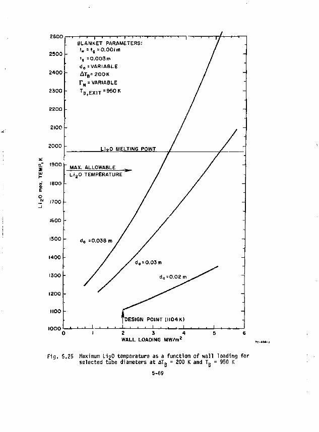
2600

2500

2400

2300

2200

2100

2000 XL

D." 1900 z w 1 -

«' 1800 o E u 1700

— i — i — i — i — i — i — i — i — i — i — r BLANKET PARAMETERS:

'« . = 'g = 0.001 m t , = 0.003m d„-VARIABLE AlB=200K

T N = VARIABLE T B , E X I T = 9 5 0 K

L i ? 0 MELTING POINT

1600

1500

1400

1300

1200 -

1100

1000

MAX. ALLOWABLE • L i 2 0 TEMPERATURE

[DESIGN POINT [1104 K) J — i • _ • I .i . . ^ _ L 2 3 4 WALL LOADING MW/m2

Fig. 5,25 Maximum LigO temperature as a function of wall loading for selected tube diameters at AT„ = 200 K and Tg = 950 K

5-69

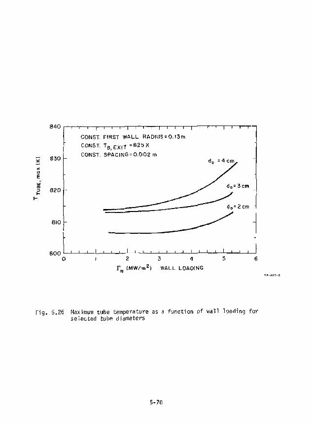
8 4 0

830

820

Q)0

8 0 0

l — i — | — i — i — ! — | — i — i — i — | — l — l — l — T

CONST. FIRST WALL RADIUS = O.I3m

CONST. T 6 E X ( T = 8 2 5 K

CONST. SPACING^ 0 .002 m

-r—i—p—|—r

3 cm

= 2 cm

. . . I -1 J I I I U l_ i i I J i_

T . ( M W / m z ) WALL LOADING N

Fig. 5.26 Maximum tube temperature as a function of wall loading for selected tube diameters

5-70

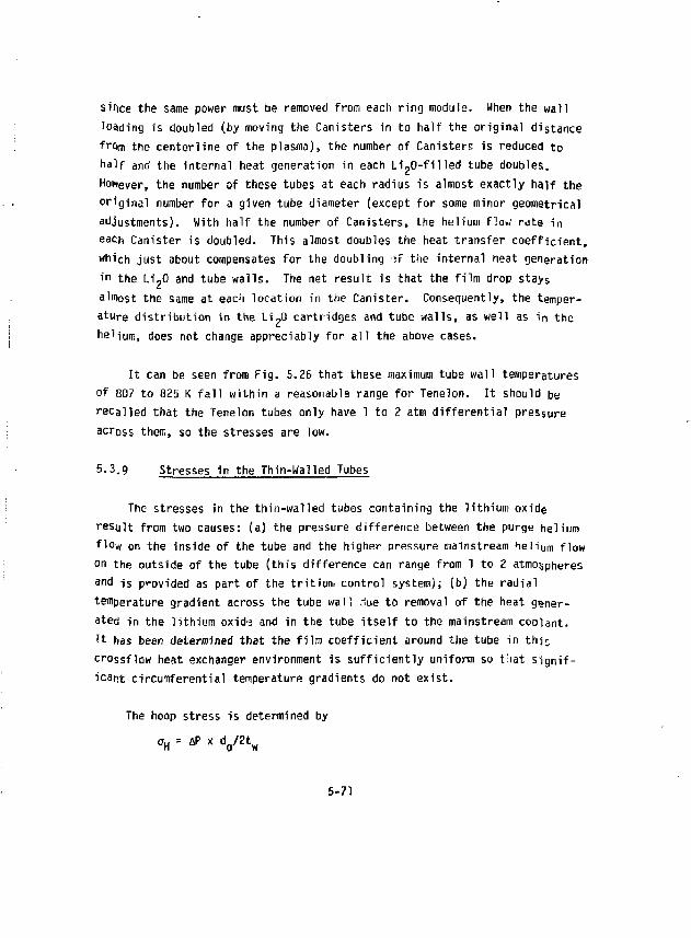
since the same power must be removed from each ring module. When the wall loading is doubled (by moving the Canisters in to half the original distance from the centerline of the plasma), the number of Canisters is reduced to half and the internal heat generation in each Li"20-fi 1 led tube doubles. However, the number of these tubes at each radius is almost exactly half the original number for a given tube diameter (except for some minor geometrical adjustments). With half the number of Canisters, the helium flo*; rate in each Canister is doubled. This almost doubles the heat transfer coefficient, which just about compensates for the doubling of the internal heat generation in the Li^O and tube walls. The net result is that the film drop stays almost the same at each location in the Canister. Consequently, the temper­ature distribution in the Li ?0 cartridges and tube walls, as well as in the helium, does not change appreciably for all the above cases.

It can be seen from Fig. 5.26 that these maximum tube wall temperatures of 8D7 to 825 K fall within a reasonable range for Tenelon. It should be recalled that the Tenelon tubes only have 1 to 2 atm differential pressure across them, so the stresses are low.

5.3.9 Stresses in the Thin-walled Tubes

The stresses in the thin-walled tubes containing the lithium oxide result from two causes: (a) the pressure difference between the purge helium flow on the inside of the tube and the higher pressure mainstream helium flow on the outside of the tube (this difference can range from 1 to 2 atmospheres and is provided as part of the tritium control system); (b) the radial temperature gradient across the tube wall rlue to removal of the heat gener­ated in the lithium oxids and in the tube itself to the mainstream coolant. ?t has been determined that the film coefficient around the tube in thj-crossflow heat exchanger environment is sufficiently uniform so that signif­icant circumferential temperature gradients do not exist.

The hoop stress is determined by a H - fiP x d Q/2t w

5-71

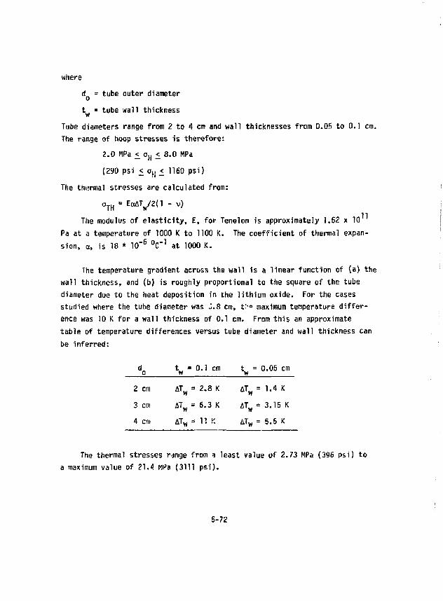
where d = tube outer diameter o t = tube wall thickness w

Tube diameters range from 2 to 4 cm and wall thicknesses from O.OB to 0.1 cm. The range of hoop stresses is therefore:

2.0 MPa < o H < 8.0 MPa (290 psi <_ oj, <_ 1160 psi)

The thermal stresses are calculated from: o T H = EccATw/2(l - v}

The modulus of elasticity, £, for Tension is approximately 1.52 x 10 Pa at a temperature of 1000 K to 1100 K. The coefficient of thermal expan­sion, a, is 18 * 10" 6 0 C _ 1 at 1000 K.

The temperature gradient across the wall is a linear function of (a) the wall thickness, and (b) is roughly proportional to the square of the tube diameter due to the heat deposition in the lithium oxide. For the cases studied where the tube diameter was J.8 cm, t.'-° maximum temperature differ­ence was 10 K for a wall thickness of 0.1 cm. From this an approximate table of temperature differences versus tube diameter and wall thickness can be inferred:

d„ t„ = 0.1 cm t = 0.0S cm o w w 2 cm AT W = 2.8 K AT W = 1.4 K 3 cm AT W = 6.3 K AT W = 3.15 K 4 cm AT W = 11 K AT W = 5.5 K

The thermal stresses range from a least value of 2.73 MPa (396 psi) to a maximum value of 21.4 MPa (3111 psi).

5-72

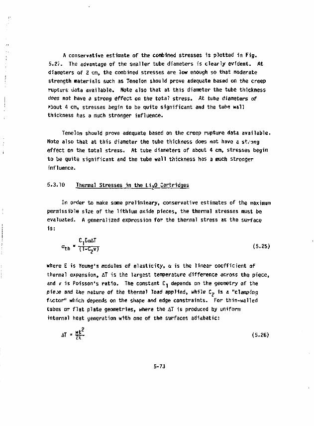
A conservative estimate of the combined stresses is plotted in Fig. 5.25. The advantage of the smaller tube diameters is clearly evident. At diameters of 2 cm, the combined stresses are low enough so that moderate strength materials such as Tenelon should prove adequate based on the creep rupture data available. Note also that at this diameter the tube thickness does not have a strong effect on the total stress. At tube diameters of ?bout 4 cm, stresses begin to be quite significant and the tube wall thickness has a much stronger influence.

Tenelon should prove adequate based on the creep rupture data available. Note also that at this diameter the tube thickness does not have a strong effect on the total stress. At tube diameters of about 4 cm, stresses begin to be quite significant and the tube wall thickness has a much stronger influence.

5.3.10 Ihermal Stresses in the LigO Cartridges

In order to make some preliminary, conservative estimates of the maximum permissible size of the lithium oxide pieces, the thermal stresses must be evaluated. A generalized expression for the thermal stress at the surface is:

C^EoAT ath = (1-C2v) < 5' 2 5 )

where E is Young's modules of elasticity, a is the linear coefficient of thermal expansion, AT is the largest temperature difference across the piece, and v is Poisson's ratio. The constant C 1 depends on the geometry of the pieje and the nature of the thermal load applied, while C 2 is a "clamping factor" which depends on the shape and edge constraints. For thin-walled tubes or flat plate geometries, where the AT is produced by uniform internal heat generation with one of the surfaces adiabatic:

wt 2

AT=f|- (5.26)

5-73

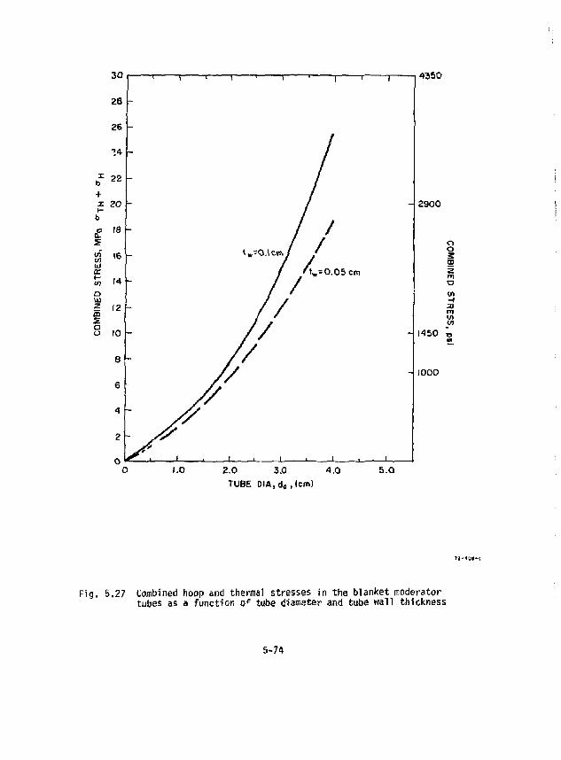
4350

2900

o 3 01

H 33 m wi V)

~ 1450 T3

- 1000

1.0 2.0 3.0 4.0 5.0 TUBE DIA,d 0,(cmJ

Fig. 5.27 Combined hoop and thermal stresses in the blanket moderator tubes as a function o* tube diaraeter and tube wall thickness

5-7*

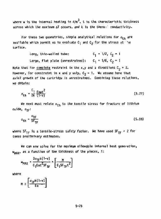
3 where VJ is the internal heating in W/m , t is the characteristic thickness across which the maximum AT occurs, and k is the thernw* conductivity.

For these two geometries, simple analytical relations for o t^ are available which permit us to evaluate C-| and Cg for the stress at 'ie surface.

Long, thin-walled tube: C, = 1/2, Cg = 1 Large, flat plate {unrestrained}: C-j = 1/6, C 2 = 1

Note that for complete restraint in the x,y and z directions C, = 2. However, for constraint in x and y only, Cg = 1 - We assume here that axial growth of the cartridge is unrestrained. Combining these relations, we obtain:

_ 1 EOtWt fr „ l

We next must relate a ^ to the tensile stress for fracture of lithium oxide, o-j-p:

Jth = W a,„ = 5 ^ (5.28) TF

where S F T F is a tensile-stress safety factor. We have used SF T F = 2 for these preliminary estimates.

We can now solve for the maximum allowable internal heat generation, W M A X , as a function of the thickness of the pieces, t:

_ 2g T F k( l -v) _ M A X C^Eaf'SF

o T F kU-v ) r M I

lEat z SF T f L C l S F T F t Z J

where

fcrT Fk(l-v)*[

5-75

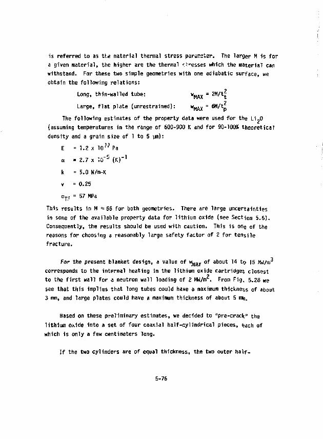
is referred to as tt.e material thermal stress parameter. The larger M is for a given material, the higher are the thermal r.Besses which the material can withstand- For these two simple geometries with one adiabatic surface, we obtain the following relations:

o Long, thin-walled tube: vm,t ~ Z M^*t Large, flat plate (unrestrained): w , ^ = 6M/t

The following estimates of the property data were used for the Li ?0 (assuming temperatures in the range of 600-900 K and for 90-100% theoretical density and a grain size of 1 to 5 um):

E = 1 . 2 x l o " Pa a = 2.7 x 'G~ 5 (K)" 1

k =5.0 W/m-K v = 0.25 o T ? = 57 MPa

This results in M =66 for both geometries. There are large uncertainties in son.e of the available property data for lithium oxide (see Section 5.6). Consequently, the results should be used with caution. This is one of the reasons for choosing a reasonably large safety factor of 2 for tensile fracture.

For the present blanket design, a value of w „ ^ of about 14 to J5 fW/m 3

corresponds to the internal heating in the lithium oxide cartridges closest to the first wall for a neutron wall loading of 2 Mw/m . From Fig, 5.28 we see that this implies that long tubes could have a maximum thickness of about 3 mm, and large plates could have a maximum thickness of about 5 mm.

Based on these preliminary estimates, we decided to "pre-cracls" the lithium oxide into a set of four coaxial half-cylindrical pieces, §ach of which is only a few centimeters long.

If the two cylinders are of equal thickness, the two outer half-

5-76

«,--%?.

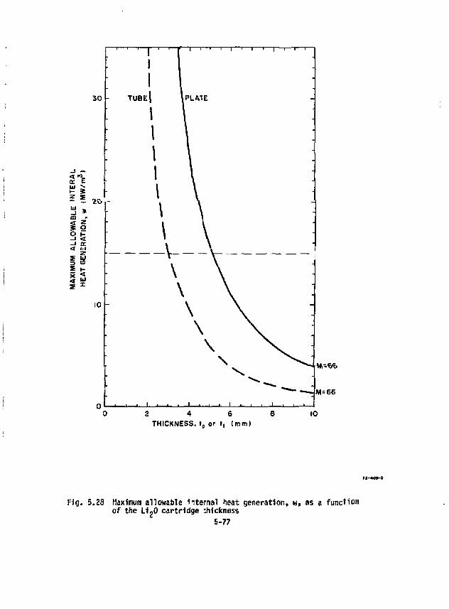
M=66

2 4 6 THICKNESS. I , or I, (mrn>

10

Fig. 5.2fl Maximum allowable internal heat generation, w, as a function of the LiJO cartridge thickness

5-77

cylinders will have f.igher thermal stresses than the inner two, since the heat flow is radially outward. This causes the outer pieces to have both the AT due to the Internal heat generation and a &T due to the heat flow from the inner pieces. Consequently, the outer half-cylindrical pieces will probably have to be somewhat thinner than the inner pieces.

The thermal stresses for this pre-cracked design lie somewhere between those of the tube and those of the .mrestrained flat plate shown on Fig. 5.28. If the half-cylinders are not tightly restrained, this design should be closer to the flat plate case than the tube caoc. Consequently, after some refinement, this geometry should insure that the thermal stresses will not cause premature failure. However, a more detailed 3-D computer stress analysis for the final geometry is certainly warranted as soon a- more reliable LipO data are available.

5.3.11 Pressure Losses and Pumping Power

A series of schematics of the network of coolant pipes from the reactor blanket Canister to the primary side of the intermediate heat exchanger is shown in Figs. 5.29 through 5.33.

Calculations were run to estimate the total pressure drop and pumping power for the entire blanket coolant circuit including the primary side of the IHX. The equations used for these different losses follow.

The frictional pressure drop for flow in pipes is defined by:

where «, = pipe length, m d = pipe Inside diameter, m

3 p = helium gas density, kg/nr

5-78

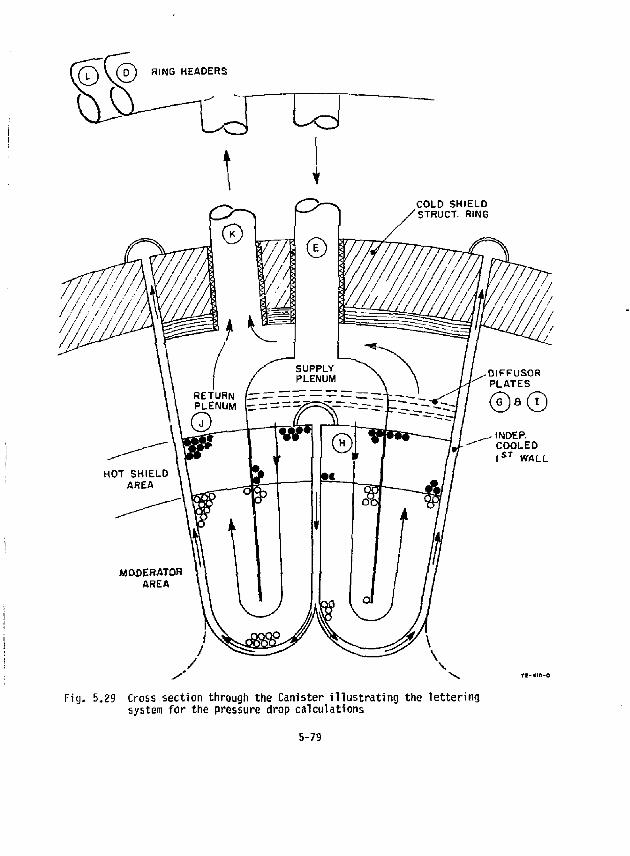
Fig. 5,29 Cross section through the Canister illustrating the lettering system for the pressure drop calculations

5-79

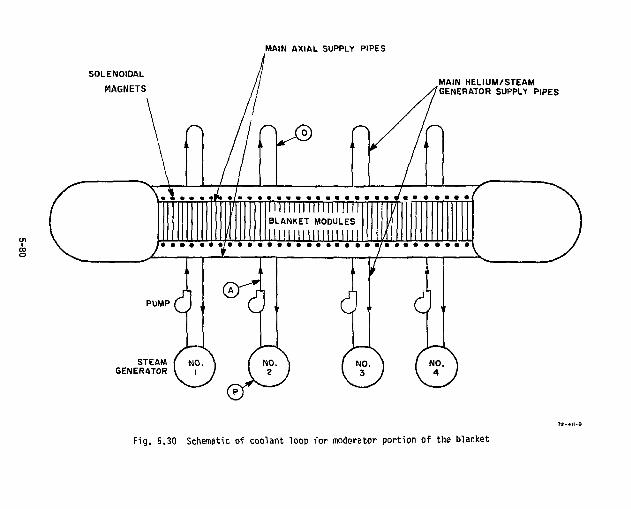
MAIN AXIAL SUPPLY PIPES

SOLENOIOAL

MAGNETS

cv®

iniii i i i i i i i i i i i BLANKET MODULES

PUMP

STEAM GENERATOR

0\ ®3l rt

Ql

NO. JS © (FJ

MAIN HELIUM/STEAM GENERATOR SUPPLY PIPES

NO.

X

Fig. 5.30 Schematic of coolant loop for moderator portion of the blanket

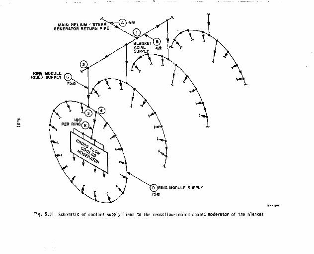
MAIN HELIUM ' STEAM GENERATOR RETURN PIPE

RING MODULE RISER SUPPLY (.C

MODULE SUPPLY

Fig, 5.31 Schematic of coolant supply lines to the crossflow-cooled cooled moderator of the blanket

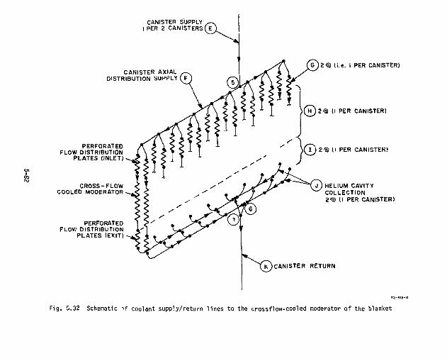
CANISTER SUPPLY I PER 2 CANISTERSfE

CANISTER AXIAL DISTRIBUTION SUPPLY ( F

PERFORATED FLOW DISTRIBUTION

PLATES (INLET)

CROSS-FLOW COOLED MODERATOR

PERFORATED FLOW DISTRIBUTION

PLATES (EXIT)

2 ® (i.e. I PER CANISTER)

2<3 (I PER CANISTER)

2 ® (I PER CANISTER!

J j HELIUM CAVITY COLLECTION 2-a (I PER CANISTER)

K ) CANISTER RETURN

Fig. 5.32 Schematic ->f coolant supply/return l ines to the crossf low-cooled moderator of the blanket

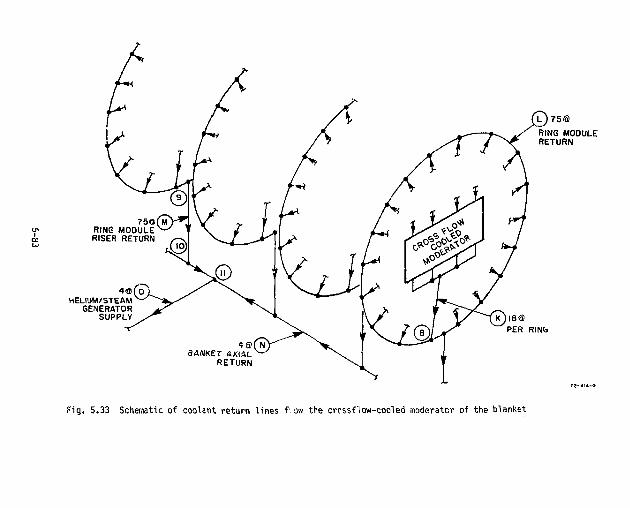
75G RING MODULE RISER RETURN

4«[o HELIUM/STEAM

GENERATOR SUPPLY

8AWKCT AXIAL RETURN

RING MODULE RETURN

PER RING

Fig. 5.33 Schematic of coolent return lines f'. om the crcssf'low-cooled moderatcr of the blanket

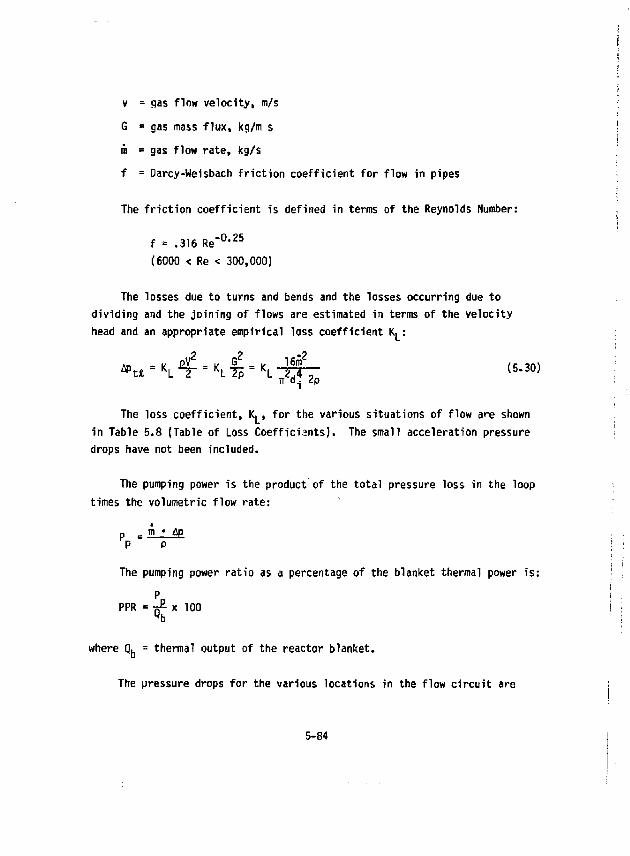
v - gas flow velocity, m/s G = gas mass flux, kg/m s m = gas flow rate, kg/s f = Darcy-Weisbach friction coefficient for flow in pipes

The friction coefficient is defined in terms of the Reynolds Number:

f = .316 R e " 0 " 2 5

(6000 < Re < 300,000)

The losses due to turns and bends and the losses occurring due to dividing and the joining of flows are estimated in terms of the velocity head and an appropriate empirical loss coefficient K. :

ir d i Zp

The loss coefficient, K., for the various situations of flow are shown in Table 5.8 (Table of Loss Coefficients). The small acceleration pressure drops have not been included.

The pumping power is the product of the total pressure loss in the loop times the volumetric flow rate:

p _ m • ap P P

The pumping power ratio as a percentage of the blanket thermal power is: P n

PPR = jf- x 100 g b

where Q. = thermal output of the reactor blanket.

The pressure drops for the various locations in the flow circuit are

5-84

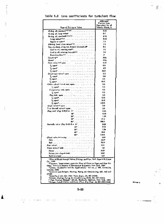
Table 5.8 Loss coefficients for turbulent flow

Typr of Filling ot Valve

Additional Fritiinn Lou.

Equivalent No. of Velocity Heads. K

*.S-ciej ell slirxUrd ••»••»•« 0.35 0.2 0 7 3 0.(5 :.3 1.5 0 4 1 0 1 0 1" 004 004 0 ) 7 0.9 4 S

24.0 23 2 6

0.35 0.2 0 7 3 0.(5 :.3 1.5 0 4 1 0 1 0 1" 004 004 0 ) 7 0.9 4 S

24.0 23 2 6

0.35 0.2 0 7 3 0.(5 :.3 1.5 0 4 1 0 1 0 1" 004 004 0 ) 7 0.9 4 S

24.0 23 2 6

Tee. standard, along run, branch blanked off* . . . .

0.35 0.2 0 7 3 0.(5 :.3 1.5 0 4 1 0 1 0 1" 004 004 0 ) 7 0.9 4 S

24.0 23 2 6

0.35 0.2 0 7 3 0.(5 :.3 1.5 0 4 1 0 1 0 1" 004 004 0 ) 7 0.9 4 S

24.0 23 2 6

0.35 0.2 0 7 3 0.(5 :.3 1.5 0 4 1 0 1 0 1" 004 004 0 ) 7 0.9 4 S

24.0 23 2 6

0.35 0.2 0 7 3 0.(5 :.3 1.5 0 4 1 0 1 0 1" 004 004 0 ) 7 0.9 4 S

24.0 23 2 6

0.35 0.2 0 7 3 0.(5 :.3 1.5 0 4 1 0 1 0 1" 004 004 0 ) 7 0.9 4 S

24.0 23 2 6

0.35 0.2 0 7 3 0.(5 :.3 1.5 0 4 1 0 1 0 1" 004 004 0 ) 7 0.9 4 S

24.0 23 2 6

0.35 0.2 0 7 3 0.(5 :.3 1.5 0 4 1 0 1 0 1" 004 004 0 ) 7 0.9 4 S

24.0 23 2 6

0.35 0.2 0 7 3 0.(5 :.3 1.5 0 4 1 0 1 0 1" 004 004 0 ) 7 0.9 4 S

24.0 23 2 6

0.35 0.2 0 7 3 0.(5 :.3 1.5 0 4 1 0 1 0 1" 004 004 0 ) 7 0.9 4 S

24.0 23 2 6

0.35 0.2 0 7 3 0.(5 :.3 1.5 0 4 1 0 1 0 1" 004 004 0 ) 7 0.9 4 S

24.0 23 2 6

'/, open' Glolie valve/.' Iirvel seat, open . .

|.j open* Composition M?al, open . . . .

% °P">* Plug dill, open .' v. .

'/. opcn» % °P">* V. <JP"l*

Angle valve,"* open , Y or btoworT valve,*-1 open . . . Plug coci'(Fig 5-39)0= 5' , .

10" . . 20" . . 40" . . 60' . .

Butterfly valve' (Fig. 5-401 » = 5" 10" 20* 40" 60"

Cllecpl vaiVe,**''"siv|iig-Disk Ball

Foot valve* Water meter." disli

Tislon Botary (stai.shaped disk) . . . . Turr'ne-wlieel

4.3 21.0 6.0 9 5 60 65 90

130 360

112.0 2 0 3.0 005 029 1S6

17.3 206.0

0.24 052 1.54

108 HBO

2.t» 10.0" 70.0" 150 7.C

IS.fr 100-

tar •Flow oJ Fluids through Valves. Fillings, and Pip*, Trrh. Paper 410, Crane

Co.. 1969. "Freeman, "Experiments upon tlie Flow of Water in Pipes and Pipe Fit­

tings," American Society ol Mechanical Engineers. New York, 1941. rCil»on, "Hydraulic* and lis Applications." 5l)i ed„ p. 250, ConsuMe,

London. 1952. 'CieseiLe and Badgelt, Heating. Piping Air Conrfin'ontng. 4(6), 443-447

(1932). •Cicsrrle,/ Am. fee. Hal. Vent, frig™., 32, 46} (1926). 'Oilman, /'rafinfc Pirrinf Air Cc-rrfirimiinr, 57(4), 141-147 (195S). '"Pipe Friction Manual." 3d ed., Hydraulic Institute, New York, 1961. 'Hoopes, kakoff, CI u l e . and Drew, Chan. Inf. Prog.,. 44.691-696 (1948).

5-85

shown in Table 5.9 for the frictional pressure drops and in Table S.10 for the pressure drops due to bends and turns, etc. The location of these pressure drops may be found by referring to the appropriate figure. The circled letters in the figures refer to frictional pressure drops and the circled numbers refer to turns and bends.

The total pressure drop is about 57 kPa {^ 8.3 psi), a modest number that could possibly be reduced further by optimization. In terms of percen­tage of the blanket thermal power, about 1.3% is required to overcome these flow losses. It can be noted that the blanket/shield part of this flow circuit, i.e., the crossflow heat exchanger, accounts for less than 25% of the total pressure loss, whereas more than 50% is attributable to losses due to turns, bends, dividing flows and joining flows.

The relatively high velocity flow in pipes that terminates in a plenum section with an abrupt expansion of flow area is a cause for concern that needs further study. We have introduced diffusers in these regions that are used to smooth out the flow and distribute it uniformly to the blanket. They have not been designed in detail but it has been assumed that the perfora­tions in the diffusor plates can be v;>-ied axially to balance the flow.

5.3.12 Heat Losses Through Insulation and Pipe Lagging

The coolant pipes in the immediate area of the reactor must, of neces­sity, be well insulated and thermally shielded to keep heat losses at a minimum. The energy transfer to components such as the superconducting coils must be guarded against since roughly 10 watts of refrigeration power are required to remove 1 watt of energy inadvertantly deposited in the liquid nitrogen coolant surrounding the helium-cooled coils. This is a serious design problem beyond the scope of this report but solutions must center on operating the rea^.or in a vacuum or near-vacuum environment so as to avoid the setting up of convective heat transfer loops and intolerable heat transfer.

5-86

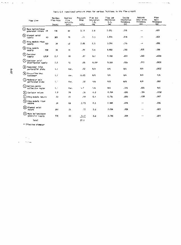
Table 5.9 Functional pressure drops fo r various tocatfons in Che f low c i r c u i t

Pipe Line Maximum Flow Rate

(kq/s)

Average Flow Velocity (m/5)

Pressure Drop

(kPa)

Piqe and Insulation

I.D. (ml

Pipe and Insulation

O.D. (m)

Inside Insulation Thickness

(m)

Outside Insulation Thickness

(ml

Pipe Wall

Thickness (ml

( A ) Main helium/steam generator return 4@ 736 60 3.12 2.0 2.072 .015 -- .021

(i) Blanket axial supply 40 368 19 .17 2.0 2.074 .016 " .021

(jf) Ring module riser supply 750 39 52 2.05 0.5 0.544 .016 - .006

QT) Ring module supply 750 20 16 .44 0.5 0.662 .050 .025 .006

(T) Canister supply 13509 2.2 18 .27 0.2 0.306 .030 .020 .0028

Q Q Canister axial distribution supply 2.1 12 .05 0.25* 0.334 .026 .013 .003Z

QT) Moderator inlet perforation plate 1.1 Var. .02 N/A N/A N/A N/A .0032

( H ) Cross-flow heat exchanger 1.1 Var. 13.65 N/A N/A N/A N/A N/A

(7) Moderator exit perforated plate 1.1 Var. .02 H/A N/A N/A N/A .003

(j) Helium cavity collection region 1.1 Var. •v. 0 N/A N/A .025 .025 N/A

M O Canister return 2.2 24 .56 0.2 0.384 .065 .024 .0032

(T) Ring module return 20 21 .59 0.5 0.756 .093 .028 .007

[MJ Ring module riser return 39 68 2.73 0.5 0.564 .026 -- .006

( N ) Blanket axial return 368 25 .22 2.0 2.094 .026 -- .021

(o) Main herium/steam generator supply 736 80 4.11 2.0 2.09D .024 -- .021

Total 27.8

* Effective diameter

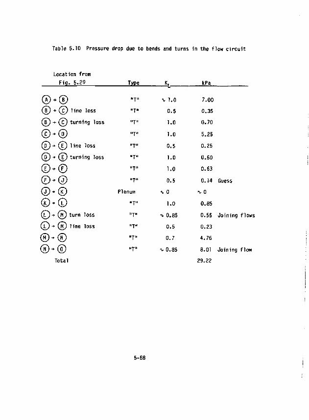
Table 5.10 Pressure drop due

Location from Fig. 5.29 Type

0,0 •T"

0 + 0 1 ine loss I I TH

0 -»- 0 turning loss H T M

©*® IITJI

0 + 0 line loss II T i l

0 + 0 turning loss M T H

©-© II T i l

0*0 II T i l

0+© Plenum

©*© It T i l

© H- 0 turn loss I ITH

© - * © line loss rrTt*

0 + 0 I I T I I

©+© HTI I

Total

bends and turns in the flow circuit

K L kPa

-u 1.0 7.00 0.5 0.35 1.0 0.70 1.0 5.25 0.5 0.25 1.0 0.50 1.0 0.63 0.5 0.14 Guess

•v, 0 -v 0

1.0 0.85 T- 0.85 0.55 Joining flows

0.6 0.23 0.7 4.76

^ 0.85 8.01 Joining flow 29.22

5-88

Once beyond the immediate area of the reactor and its evacuated chamber, the problem reduces to one of relatively simple heat transfer that permits tolerable energy balances to be made. We assume in this region that the Pipe wall is made up of both its structural components and the necessary insula­tion- Figure 5.34 illustrates a typical pipe in cross section. Following the method suggested by General Atomic, the theory is that the high temper­ature coolant is carried by an inner, essentially zero-stressed pipe filled with small-diameter pores through whicli the helium can permeate into an annular space between the inner pipe and an outer pipe that carries the structural load. The outer pipe is at a substantially lower temperature than the inner pipe due to the temperature gradient developed in the non-flowing helium in the annular space between pipes. Pressures are essentially balanced so that the inner pipe is stress free except for those stresses due to gravity forces. The outer pipe bears the brunt of the pressure-induced stresses. The annulus may be filled with a high-porosity matt insulator to prevent local convective mixing or the space may be filled only with the stagnant helium. The outer pipe is lagged further to decrease the heat loss from the system but not so much as to approach an adiabatic condition which would force the outer pipe temperature to approach the inner pipe temper­ature-

The outer diameter of the pipe can be defined in terms of the allowable heat loss, the maximum allowable temperature of the structural pipe wall* and the average bulk temperature of the helium flowing in the inner pipe. Trie average bulk temperature of the helium is determined from:

0 2m C b.in P

fraction of heat lost bj the pipe total blanket heat generation helium flow rate

where f„

%

5-89

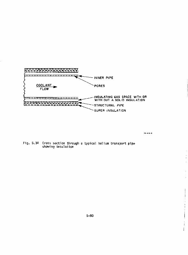
/yyyyyyyyyyyyy^L ' ' I I - I i i i i i i i i^r -^_

COOLANT FLOW

I I I I I I I I I I I l"l I I I I T

INNER PIPE

•PORES

INSULATING GAS SPACE WITH OR WITH OUT A SOLID INSULATION

•STRUCTURAL PIPE SUPER INSULATION

F ig . 5.34 Cross section through a typ ica l helium transport pipe showing insu la t ion

5-90

C = specific heat capacity of the helium T. . = bulk temperature of the helium at the inlet of the pipes b,in

The hot side insulation thickness, t. h, in the stagnant gas-filled annular space is given by the equation

^ Nj^ " w K h ^ where the thermal resistance of the inner pipe wall has been neglected and where

h = heat transfer coefficient given by Eq. (5.15) D, = outer pipe hot-side diameter (i.e., inner diameter) i, = pipe length T . = maximum inner wall temperature of the outer pipe k. . = hot side insulation thermal conductivity he cold side insulation thickness, t, , is given by

t .

where k = pipe thermal conductivity k. = cold side insulation thermal conductivity i,c T = maximum cold surface temperature of the outer pipe

The pipe wall thickness is determined by setting hoop stress for a 50-spher

equation atmosphere delta pressure equal to the )% creep stress (a) at T . from the

& * ( D h + 2 t i h ) / 2

p » c "creep

5-91

5.3.13 Canister Blanket and Hot Shield: Performance Summary and Conclusions

The details of the thermal-hydraulic performance for the FY82 reference Canister blanket design are given in Tables 5.7a-g. A simplified summary of the key data are given in Table 5.11. We can draw the following conclusions about this blanket design:

a) The concept of the use of a solid LioO breeder material inside of tubes arranged as a two-pass, cross-flow heat exchanger appears to be very attractive.

b) This arrangement separates the tritium from the main helium flow which reduces the tritium recovery problems and snakes the isolation of the tritium from the synfuel plant very effective.

c) The small purge helium flow inside the tubes for removing tritium from the Li-0 need only be at one or two atmospheres lower pressure than the main helium coolant flow to ensure that almost no tritium will get into the main flow in the event of a leak. This allows the hot tubes to be thin and still operate at very low Stress levels, since they are almost pressure balanced.

d) The closely-spaced, cross-flow tube bank arrangement results in almost uniform tube wall temperatures around the circumference and high neat transfer coefficients; this helps to avoid hot spots on the tube walls.

e) The maximum tube wall temperature is only about 810 K at the worst point (near the exit of the second breeder section); it is only about 758 K where the combined stresses are a maximum of 5.6 MPa. These stresses are very low for Tenelon.

f) The maximum and minimum Li 20 temperatures are 962 K and 666 K,

5-92

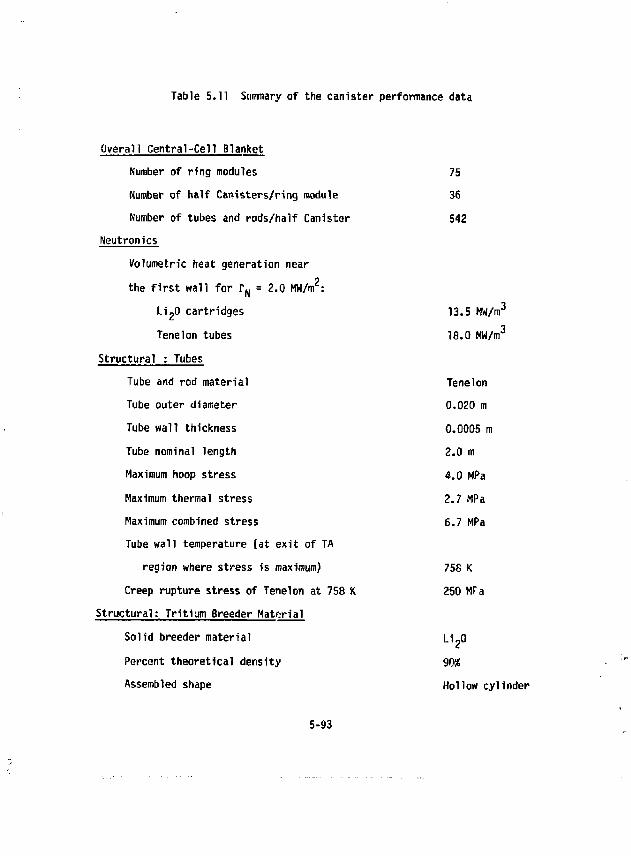
Table 5.11 Summary of the canister performance data

Overall Central-Cell Blanket Number of ring modules 75 Number of half Canisters/ring module 36 Number of tubes and rods/half Canister 542

Neutronics Volumetric heat generation near the first wall for r N = 2.0 MW/m2:

Li 20 cartridges 13.5 MW/m 3

Tenelon tubes 18.0 MW/m3

Structural : Tubes Tube and rod material Tenelon Tube outer diameter 0.020 m Tube wall thickness 0.0005 m Tube nominal length 2.0 m Maximum hoop stress 4.0 MPa Maximum thermal stress 2.7 MPa Maximum combined stress 6.7 MPa Tube wall temperature {at exit of TA

region where stress is maximum) 75S K Creep rupture stress of Tenelon at 758 K 250 Wa

Structural: Tritium Breeder Material Solid breeder material Li ?0 Percent theoretical density 90* Assembled shape Hollow cylinder

5-93

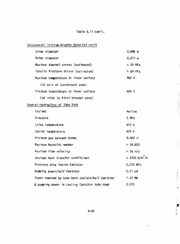
Table 5.11 con't.

Structural: Tritium Breeder Material con't Inner diameter 0.006 m Outer diameter 0.017 m Maximum thermal stress (estimated) % 35 MPa Tensile fracture stress (estimated) ^ 69 MPa Maximum temperature at inner surface 962 K

(at exit of turnaround zone) Minimum temperature at inner surface 666 K

(at inlet to first breeder zone) Thermal-Hydraulics of Tube Bank

Coolant Helium Pressure 5 MPa Inlet temperature 625 K Outlet temperature 825 K Minimum gap between tubes 0.002 m

Maximum Reynolds number -v. 34,000 Maximum flow velocity i. 16 m/s

2

Average heat transfer coefficient -\. 2000 W/m -K Pressure drop inside Canister 0.016 MPa Pumping power/half Canister 5.71 kW Power removed by tube bank coolant/half Canister 1.12 MW % pumping power in cooling Canister tube bank 0.51K

5-94

respectively^ This range of temperatures should result in good tritium release from the Li^O and low tritium inventories.

g) The fractional pressure drop across the tube bank is only 0.32%, which results in a ratio of the pumping power requireo to the thermal power removed of only 0.51%.

h) A greet deal of refinement and optimization of the tuoc- bank design is possible, since some tailoring of the tr;!?o diameters and spacings can be used to compensate for the r?ar-exponential decrease in the internal heat generation.

5-95

5.4 TRITIUM CONTROL IN THE BLANKET

5.4.1 Tritium Processing and Control

There are significant advantages associated with having the breeder material, L7,0, in tubes that isolate it from the main helium coolant flow. An obvious one is that imposition of an additional barrier protects the Li 20 from degradation by, and possible reaction with, contaminants that might intrude into the main helium coolant. The most likely contaminant is water. It could enter the main helium coolant due to a heat exchanger failure or a water-lubricated bearing failure on one of the helium circulators. The other obvious advantage is keeping the bulk of the tritium out of the main coolant. Reduced contamination of large parts of the system by tritium results. This makes maintenance easier. A high probability of reduced tritium losses is obtained. The volume of gas that must be processed in the tritium recovery system is greatly reduced, so equipment si2e can be minimized. With the reduced flow to the recovery system (that operates at room temperature), less waste heat is produced and plant efficiency is increased. Even if high temperature recovery processes are developed, all the other advantages are retained.

For adequate isolation of tritium in the high temperature regions, successful development of permeation barriers is required. Work in this area of tehcnology seems to have been stopped a few years ago. Prior to that, workers at ANL (Argonne National Laboratory) and NCSU (North Carolina State University) had both shown modest success along these lines. The most striking results were those of Tom Elleman and his co-workers at NCSU, but they were not all formally published. One of his papers gives the diffusion coefficient of tritium in a number of materials, most notably SiC. ' This can be expressed as

/-54 g!L«l\ D = 1.09 x 10" 2 exp ^ L

R f /

5-96

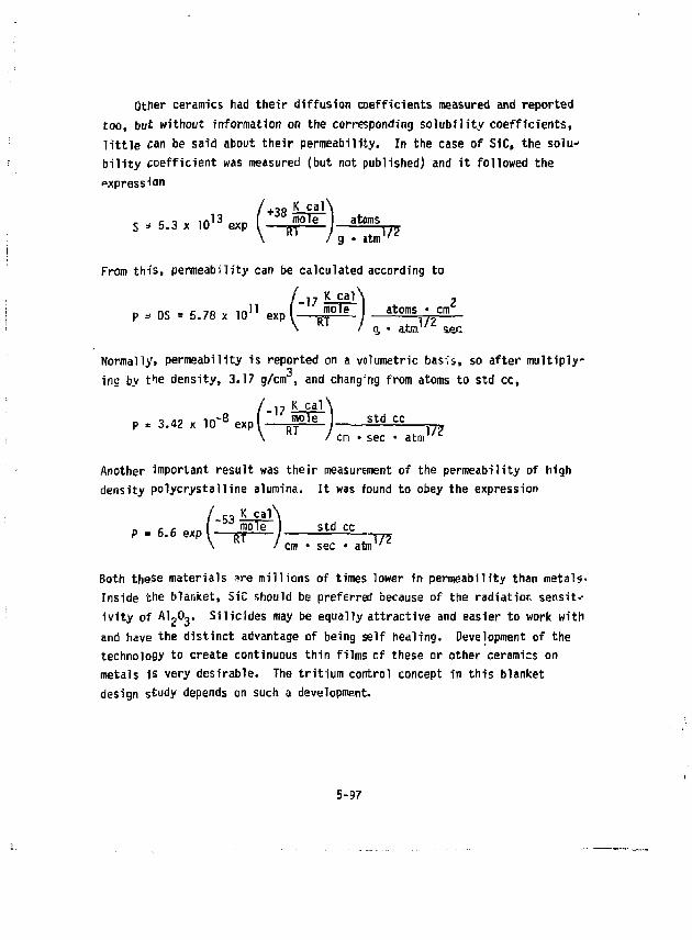
Other ceramics had their diffusion coefficients measured and reported too, but without information on the corresponding solubility coefficients, little can be said about their permeability. In the case of SiC, the solu­bility coefficient was measured (but not published) and it followed the expression

/ +3 8iLcal\ c - <; i v in 1 3 ovn I "K>le atoms

From this, permeability can be calculated according to / 77 K"A z

P * DS = 5.78 x 10 1 1 e x p l — # ^ atoms -cm \ K l / <j • aim1'* sec

Normally", permeability is reported on a volumetric basis, so after multiply-ins by the density, 3.17 g/cm , and changng from atoms to std cc,

17 K c a 1 \ P = 3.42 x 10 ° exp -8 mole std cc

R T /cm • sec • atm 1 / E

Another important result was their measurement of the permeability of high density polycrystalline alumina. It was found to obey the expression

/ 5 3 K cal\ D - « f, ovn m o 1 e std cc p = 6.6 exp l *rj I rp,

\ R T / cm • sec • atm 1 / 2

Both these materials sre millions of times lower in permeability than metals-Inside the blanket, SiC should be preferred because of the radiation sensit--ivity of A 12°3" filicides may be equally attractive and easier to work with and have the distinct advantage of being self healing. Development of the technology to create continuous thin films cf these or other ceramics on metals is very desirable. The tritium control concept in this blanket design study depends on such a development.

5-97

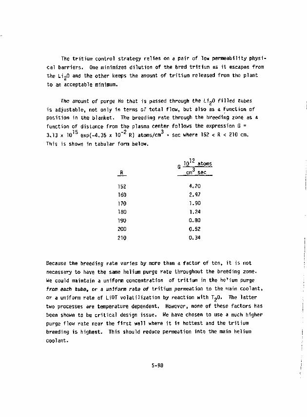
The tritium control strategy relies on a pair of low permeability physi­cal barriers. One minimizes dilution of the bred tritium as it escapes from the LipO and the other keeps the amount of tritium released from the plant to an acceptable minimum.

The amount of purge He that is passed through the LioO filled tubes is adjustable, not only in terms o" total flow, but also as a function of position in the blanket. The breeding rate through the breeding zone as a function of distance from the plasma center follows the expression G = 3.13 x 1 0 1 5 exp(-4.35 x 10" 2 R) atoms/cm3 = sec where 152 < R < 210 cm. This is shown in tabular form below.

R „ 1 0 1 2 atoms G 3 cm sec

152 4.20 160 2.97 170 1.90 180 1.24 190 0.80 200 0.52 210 0.34

Because the breeding rate varies by more than a factor of ten, it is not necessary to have the same helium purge rate throughout the breeding zone. We could maintain a uniform concentration of tritium in the helium purge from each tube, or a uniform rate of tritium permeation to the wain coolant, or a uniform rate of LiOT volatilization by reaction with TgO. The latter two processes are temperature dependent. However, none of these factors has been shown to be critical design issue. We have chosen to use a much higher purge flow rate near the first wall where it is hottest and the tritium breeding is highest. This should reduce permeation into the main helium coolant.

5-98

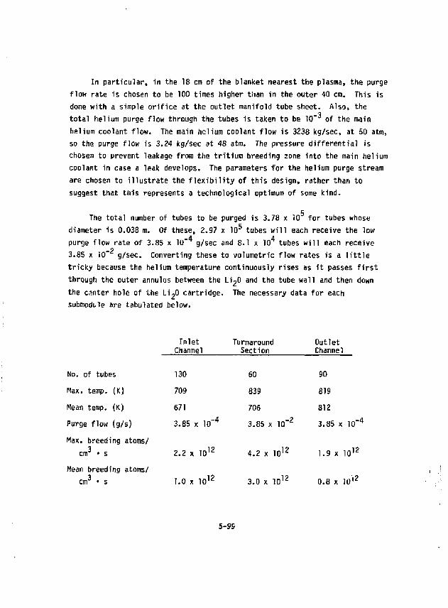
In particular, in the 18 cm of the blanket nearest the plasma, the purge flow rate is chosen to be 100 times higher than in the outer 40 cm. This is done with a simple orifice at the outlet manifold tube sheet* Also, the total helium purge flow through the tubes is taken to be 10 of the main helium coolant flow. The main helium coolant flow is 3238 kg/sec, at 50 atm, so the purge flow is 3.24 kg/sec at 48 atm. The pressure differential is chosen to prevent leakage from the tritium breeding zone into the main helium coolant in case a leak develops. The parameters for the helium purge stream are chosen to illustrate the flexibility of this design, rather than to suggest that this represents a technological optimum of some kind.

5 The total number of tubes to be purged is 3.78 x 10 for tubes whose diameter is 0.038 m. Of these, 2.97 x 10 5 tubes will each receive the low purge flow rate of 3.85 x 10" g/sec and 8.1 x 10 tubes will each receive 3.85 x 10 g/sec. Converting these to volumetric flow rates is a little tricky because the helium temperature continuously rises as it passes first through the outer annulus between the Li,0 and the tube wall and then down the canter hole of the Li^O cartridge. The necessary data for each submodtle are tabulated below.

Inlet Turnaround Outlet Channel Section Channel

No. of tubes 130 60 90 Max. temp. (K) 709 839 819 Mean temp. (K) 671 706 812 Purge flow (g/s) 3.85 x 10" 4 3.85 x 10" 2 3.85 x 10" 4

Max. breeding atoms/ cm 3 • s 2.2 x 1 0 1 2 4.2 x 1 0 1 2 1.9 x 1 0 1 2

Mean breeding atoms/ cm 3 • s 1.0 x 1 0 1 2 3.0 x 1 0 1 2 0.8 x JO' 2

5-99

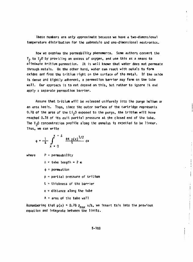
These numbers are only approximate because we have a two-dimensional temperature distribution for the submodule and one-dimensional neutronics.

Now we examine the permeability phenomenon. Some authors convert the T 2 to T 20 by providing an excess of oxygen, and use this as a means to eliminate tritium permeation. It is well known that water does not permeate through metals. On the other hand, water can react with metals to form oxides and free the tritium right on the surface of the metal. If the oxide is dense and tightly adherent, a permeation barrier may form on the tube wall. Our approach is to not depend on this, but rather to ignore it and apply a separate permeation barrier.

Assume that tritium will be released uniformly into the purge helium or an area basis. Then, since the outer surface of the cartridge represents 0.78 of the area of the Li-0 exposed to the purge, the tritium will have reached 0.78 of its exit partial pressure at the closed end of the tube. The TpO concentration profile along the annulus is expected to be linear. Thus, we can write

• --J-/"' i^O^dx x = 0

where P = permeability a - tube length = 2 m $ - permeation p = partial pressure of tritium t = thickness of the barrier x = distance along the tube A = area of the tube wall

Remembering that p(x) = 0.78 p__„ x/£, we insert this into the previous max

equation and integrate between the limits.

5-100

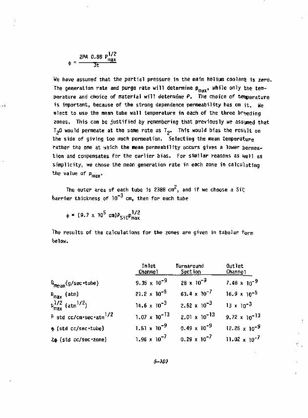
2PA 0.88 P \ [ 1 . _ max * 3t

We have assumed that the partial pressure in the main heliun coolant is zero. The generation rate and purge rate will determine p m a x , while only the tem­perature and choice of material will determine P. The choice of ternperature is important, because of the strong dependence permeability has on it, Me elect to use the mean tube wall temperature in each of the three breeding zones. This can be justified by remembering that previously we assumed that T^O would permeate at the same rate as T~. This would bias the result on the side of giving too much permeation. Selecting the mean temperature rather the one at which the mean permeability occurs gives a lower Permea­tion and compensates for the earlier bias. For similar reasons as well as Simplicity, we chose the mean generation rate in each zone in calculating the value of P m a x .

The outer area of each tube is 2388 cm , and if we choose a Si'C barrier thickness of 10" cm, then for each tube

* = (9.7 x 10 5 a ) P S i c P ; g

The results of the calculations for the zones are given in tabular form 'ie low.

Inlet Channel

Turnaround Section

Outlet Channel

( W a n ( 9 / s e c * t u b e > 9.35 x 10"9 28 x 10"3 7.48 x l o " 9

fimax < a t m ) 21.2 x 10"6 63.4 x 10" 7 16.9 x i o " 5

C c-1/2> 14.6 x 70" 3 2.52 x 10"3 13 x l o - 3

1 /2 f std cc/cm'secatm ' 1.07 x 10" 1 3 2.01 x 10" 1 3 9.72 x l o - 1 3

$ (std cc/sec«tube) 1.51 x 10~9 0.49 x 10" 9 12.25 x 10" 9

S$ (std cc/sec«zone) 1.96 x 10"7 0.29 x 10"7 11.02 x 10" 7

5-W?

The sum of the figures in the last line give the total for half of a submodule. Multiplying this by 2 x 18 x 75 gives the total for the blanket which is 3.6 x 10 std cc/sec. It may be noted that a reduction in total permeation could probably have been achieved by using a higher purge rate in the outlet channel and a lower purge rate in the turnaround section.

The partial pressure in the main coolant was assumed to be zero for this permeation calculation. Using the calculated rate of 3.6 x 10" 3 std cc/sec and the processing removal rate from the main coolant, this assumption can be verified. At steady state, the rate that tritium permeates into the main coolant must be equal to the rate at which it is removed. The removal rate consists of the processing removal rate plus the losses due to leakage and permeation into other parts of the plant. Again, we expect the losses to be minimal, so initially they are i^ored. Then,

3.6 x 10" 3 S t ^ c = nC T(fV) + losses

where fV is the volumetric flow rate going through the tritium removal pro­cessor. It is written as a fraction, f, of th3 total main helium flow, V. The concentration of tritium in the main helium flow as it enters the pro­cessor is C-p, and r\ is the fraction of this concentration that is removed in the processing section. Current technology allows n to be set at 0.99. The value of f is a design variable and is arbitrarily set at 10 . The mass flow rate is 3238 kg/sec, so at 50 atm, the volumetric flow rate is 3.63 x 10 cm sec. Substituting above, the concentration of tritium in the main helium is calculated to be 1.0 x 10" atm. This is a negligible "back pressure" for the permeation calculation, so the original approximation is justified and a second iteration is unnecessary.

Now we go to the next step and examine the amount of tritium that gets into the steam cycle that is the other side of the intermediate heat exchanger (IHX). Again, we will have the opportunity to check the validity of our assumption that losses can be ignored. The intermediate heat exchanger handles all of the thermal energy from the reactor, including the

5-102

direct converter. The methods for keeping tritium out of the direct conver­ter have not been established. Tritium-free coolants for beam dumps appear feasible, so we assume here that the helium from the direct converter ha s

the same tritium concentration as the blanket helium coolant.

The total thermal load on the He/steam IHX is 3780 MW. The first wall helium coolant is delivered at 625 K and falls to 525 K. The blanket and direct converter helium are delivered at 825 K and drop to 625 K. On the water (or steam) side, the temperatures range from 50 K to 200 K lower in temperature due to the film and tube wall drops that contribute to the over-•??? tewi tr<wfsfer coefficient. Most of the temperature drop is or> the belim side, so we will make the estimate that the IHX wall temperature is 30 (< below the helium temperature. These figures will be used to estimate the heat exchanger area and subsequently the permeation of tritium into the steain cycle. Because the helium system runs at 50 atm or 750 psi and the steam system runs above 1200 psi, any leaks that occur in the IHX will riot add tritium to the steam system. The loss question really is restricted to permeation.

In the section of this report on thermal interfacing, it is clear that no single temperature properly represents the IHX. Furthermore, the he«t transfer mechanism is not uniform on the steam side. Sometimes water i= present, sometimes it is superheated steam. Consequently, the area required to transfer a given heat load is also a variable.

This calculation will turn out not to be a critical one, so from Fig. 4, w§ will choose an overall U and &T to represent the IHX, and evaluate the Permeation at the average outside wall temperature, which is 30 K below the Average He temperature. The outside wall is where the permeation barrier is located. The assumed v?lues are U f l V E = 1000 w/m • K and AT. = 50 K, so knowing that Q = 3780 MW, the area is calculated to be 75,600 m . Although the surface temperature ranges from 495 K to 795 K, only the surface area at relatively high temperaturs contributes to the permeation. Alumina is oqr choice of material barrier on the IHX and we select a barrier 10"3 cm

5-103

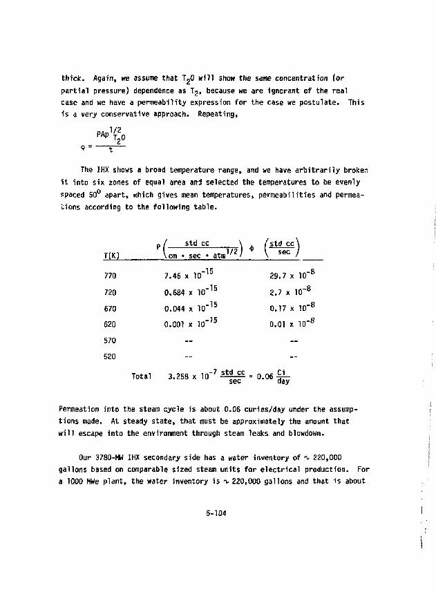
thick. Again, we assume that T 20 wi)J show the same concentration (or partial pressure) dependence as T 2, because we are ignorant of the real case and we have a permeability expression for the case we postulate. This is a very conservative approach. Repeating,

"-'ft * = i

The IHX shows a broad temperature range, and we have arbitrarily broken it into six zones of equal area and selected the temperatures to be evenly spaced 50° apart, which gives mean temperatures, permeabilities and permea­tions according to the following table.

std cc T(K) 1/2 *

\cm • sec • atm ' / ^ sec /

770 7.46 x 10" 1 5 29.7 x 10" 8

720 0.6e4 x 10" 1 5 2.7 x 10" 8

670 0.044 x 10" 1 5 0.17 x 10" 8

620 0.001 x 10"' 5 Q.01 x 10" 8

570 — — 520 — —

Total 3.258 x 10" 7 std cc _ sec °-06£y-

Permeation into the steam cycle is about 0.06 curies/day under the assump­tions made. At steady state, that must be approximately the amount that will escape into the environment through steam leaks and blowdown.

Our 3780-MW IHX secondary side has a water inventory of -*- 220,000 gallons based on comparable sized steam units for electrical production. For a 1000 HWe plant, the water inventory is *v 220,000 gallons and that is about

5-104

3500 KW t h. The makeup rate is as low as 77,000 gallons per day. Thus, the blowdown (and to a smaller extent leakage) removes a third of the water inventory per day. Consequently, the steady-state inventory of the steam plant is in the neighborhood of 0.18 curies. On a weight basis, this is about 6 x 10" . The amount of tritium that gets into the chemical plant will surely be a small fraction of that in the steam cycle, and it will be diluted by a very large flow of water into, and hydrogen out of, the thermo-_3 chemical plant. If we assume a concentration drop of 10 or more, we are barely above the background level of tritium in the biosphere. It is detect­able only with extraordinary procedures.

5.4.2 Tritium Inventory

Tritium inventory in the reactor blanket was investigated. The calcu­lated value is under 1 kg, and if our assumptions are correct and our approx­imations are reasonably valid, it should be a good number for this design.

The inventory is strongly influenced by local temperature, both through­out the blanket in general as well as across the individual Li^O cartridges inside each tube. In a real sense, it is a two-dimensional problem in two different regimes of size, and they are superimposed on one another. The strong dependence on temperature results from the exponential temperature dependence of tritium's diffusion coefficient in Li'oO. Another crucial parameter that must be known is the local tritium breeding rate. This, too, is a two-dimensional problem, particularly with our fluted first wall and cylindrical blanket configuration. So far these calculations are available only for one-dimensional geometries. Finally, the inventory depends on the amount and morphology of the Li~0 itself.

Let us first direct our attention to the lithium oxide. The Li g0 is shaped into hollow half cylinders. They are of radii such that they can be "nested" to form a fairly thick-walled hollow cylinder. When these pieces are formed, they are pressed from powder and then fired to create pieces that are ver^ near 100* theoretical density. After conventional ceramic

5-105

fabrication, stacks of these pieces are made to be 10% porous in either of two rather unusual ways.

The first is to use a modification of the "pore former" technique. Very fine fibers would be chopped to short lengths of a millimeter or two. They would be in the micron range of diameters and have two chemical qualities. They wouldn't react with LipO, even at high temperature. They also could be burneu or evaporated out, leaving a channel, if exposed to hot pure oxygen or some other suitable environment. That might just be high temperature in high vacuum, if the fiber is to evaporate. Any number of hydrocarbon fibers might workj or cadmium, and with study other alternatives would be discovered. The chopped fibers would be premixed with the LipO powder and hot-pressed to full density. Then a light cut would be taken off the inner and outer surfaces of the cartridge part to ensure the fibers actually were connected with the outside surface. Subsequent exposure to hot oxygen or vacuum would leave a 90SS-dense, microporous ceramic body. The holes would be round^ so the tendency to sinter would be minimal.

Alternatively, an array of holes are bored radially through the Li o tube wall to allow the tritium to escape after having diffused only a short distance in the solid. This array is a rectangular pattern on 14 um centers. The hole diameter is 5 um, and these holes needn't be perfectly straight or round. This array is produced very quickly by boring a very "targe number of holes simultaneously with laser beams. The array spacing and hole dianieter were chosen to meet the requirements of Li,0 density, acceptable tritium inventory, and the ability of laser drilling technology to make the parts in a few years. Today there are commercial methods for creating porous surfaces on high speed aircraft using laser drilling. The holes are about 2 mm deep but are 50 um in diameter. People working in this field believe 5 um boles could be developed in a year or two of development time. Given the rapid progress in fiber optics, high powered lasers, and laser- based fabrication technologies, this seems like a reasonable extrapolation.

One element of an array like this is shown in Fig. 5-35. The heavy

5-106

f

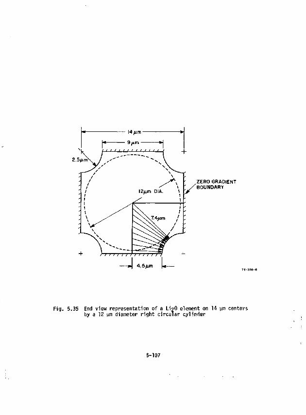
ZERO GRADIENT BOUNDARY

Fig. 5.35 End view representation of a U2O element on 14 \m centers by a 12 uni diameter right circular cylinder

5-107

lines indicate planes across which trit'um does not diffuse. This element is slightly tapered because it runs radially through the Li-O piece, hut this taper is ignored. The end planes of the element are curved because of the boundary planes on the LipO piece, and this is ignored. Now we approximate this element as a solid right circular cylinder of infinite length. The distance a tritium atom must diffusa ranges from 4.5 nn to 7.4 um, depending on where the atom is formed. For the purpose of estimating the tritium inventory, we set this element's distance for diffusion purposes to be 6 fin, which will be the radius of the cylinder that approximates the element. To account for the fact that much of the element's boundary does not allow tritium to escape, we increase the concentration of tritium in proportion to the fraction of inactive boundary, while using mathematics appropriate to a fully active boundary. Some of these approximations are more appealing than others. A full two- or three-dimensional numerical model with good data is needed to exactly calculate the behavior that will be observed. Under the circumstances the approach seems reasonable.

The calculation i :arts by writing the diffusion equation with a continuous uniform source term, 5.

After integrating once and using the fact that dc/dr = 0 at r = 0, we have j£ Gr dr ~ 2D

This is integrated again, and the homogeneous boundary condition is invoked at the outer boundary» i.e., C = 0 at r• = x

C ( r ) = - | j ( r 2 - x 2 )

The inventory is obtained by integrating the concentration over the volume of the element and applying the fudge factor, f, for the partially blocked boundary:

5-108

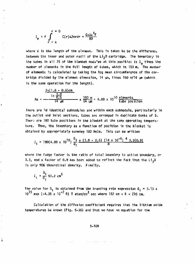
r = 0 4

I e = f f C(r)i2nrdr = Gl^* f

r = x

where «, is the length of the elenient. This is taken to be the difference between the inner and outer radii of the LigO cartridge. The inventory in the tubes in all 75 of the blanket modules at this position is JL times the number of elements in the full length of tubes, which is 150 m. The number of elements is calculated by taking the log mean circumference of the car­tridge divided by the element dimension, 14 urn, times 150 m/14 \m (which is the same operation for the length).

2n(1.8 - 0.5)cm In '*8

N. _ TF5 150 m _ . flfl l n 1 0 elements ™ e " 14 um x TTim ' 4 , a B * u tube position

There are 18 identical submodules and within each submodule, particularly in the outlet and inlet sections, tubes are arranged in duplicate banks of 5. Ther': are 180 tube positions in the blanket at the same operating tempera­ture. Thus, the inventory as a function of position in the blanket is obtained by appropriately summing 180 Nele. This can be written

I. = 180(4.88 x 10 1 0) ! l M l - 8 - 0 . 5 ) (14 x 10' 4) 4 3.3(0.9)

where the fudge factor is the ratio of total boundary to active boundary, or 3.3, and a factor of 0.9 has been added to reflect the fact that the Li ?0 is only 90% theoretical density. Finally,

Gi S I. = -s1 SI.2 cm 3

i

The value for G is obtained from the breeding rate expression G. = 3.13 x 1 0 1 5 exp {-4.35 x 10" 2 R) T atom/cm3 sec where 152 cm < R < 210 cm.

Calculation of the diffusion coefficient requires that the lithium oxide temperatures be known (Fig. 5-36) and that we have =tn equation for the

5-109

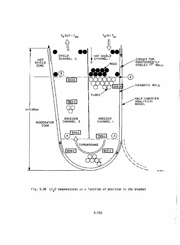
T B 0 U T = T B 6 T B I N = T B |

H=0.85m

CIRCUIT FOR INDEPENDENTLY COOLED I S T WALL

ADIABATIC WALL

HALF CANISTER ANALYTICAL MODEL

Fig. 5.36 Li^O temperatures as a function of position in the blanket

5-110

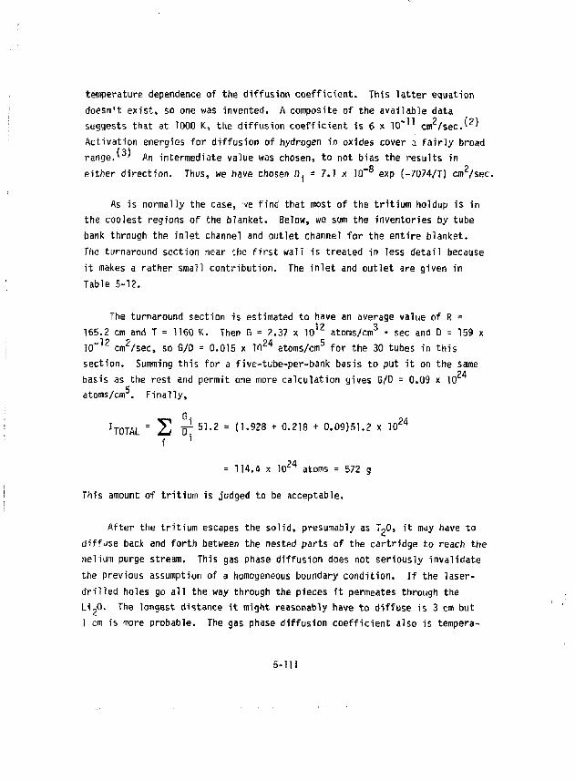
temperature dependence of the diffusion coefficient. This latter equation doesn't exist, so one was invented. A composite of the available data suggests that at 1000 K, the diffusion coefficient is 6 x 10" 1 1 c m 2 / s e c . ^ Activation energies for diffusion of hydrogen in oxides cover a fairly broad range.* ' An intermediate value was chosen, to not bias the results in either direction. Thus, we have chosen D. = 7.1 x 10 ° exp (-7074/T) cnr/sec.

As is normally the case, we find that most of the tritium holdup is in the coolest regions of the blanket. Below, we sum the inventories by tube bank through the inlet channel and outlet channel for the entire blanket. The turnaround section near the first wall is treated in less detail because it makes a rather small contribution. The inlet and outlet are given in Table 5-12.

The turnaround section is estimated to have an average value of R = 165.2 cm and T = 1160 K. Then G = 2.37 x 10 atoms/cm3 • sec and D = 159 x 10 cm2/sec, so G/D = 0.015 x 1 0 2 4 atoms/cm5 for the 30 tubes in this section. Summing this for a five-tube-per-bank basis to put it on the same basis as the rest and permit one more calculation gives G/D = 0.09 x 10

c atoms/cm . Finally,

I T 0 T A L = 2 JJ 1 51.2 = (1.928 + 0.218 + 0.09)51.2 x 1 0 2 4

= 114.4 x 1 0 2 4 atoms = 572 g

This amount of tritium is judged to be acceptable.

After the tritium escapes the solid, presumably as ToO, it may have to diffuse back and forth between the nested parts of the cartridge to reach the helium purge stream. This gas phase diffusion does not seriously invalidate the previous assumption of a homogeneous boundary condition. If the laser-drilled holes go all the way through the pieces it permeates through the Li20. The longest distance it might reasonably have to diffuse is 3 cm but 1 cm is more probable. The gas phase diffusion coefficient also is tempera-

5-111

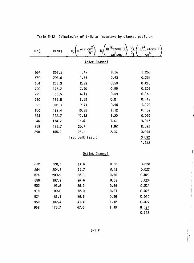
Table 5-12 Calculation of tritium inventory by blanket position

™ ••-> «W) ' fc 1 ) £ K H Inlet Channel

1.42 0.36 0.253 1.81 0.43 0.237 2.29 0.50 0.218 2.90 0.59 0.203 4.11 0.69 0.168 5.69 0.81 0.142 7.71 0.96 0.124

10.25 1.12 0.109 13.13 1.30 0.099 16.6 1.62 0.097 20.7 1.92 0.092 25.1 2.37 0.094

last bank (est.) 0.092 1.928

654 203.3 669 204.6 684 200.9 700 197.2 725 193.5 750 189.8 775 186.1 800 182.4 823 178.7 846 174.2 869 169.7 890 165.2

Outlet Channel

852 208.3 17.6 0.36 0.020 864 204.6 19.7 0.43 0.022 876 200.9 22.1 0.50 0.023 888 197.2 24.6 0.59 0.024 903 193.5 28.2 0.69 0.024 918 189.8 32.0 0.81 0.025 934 186.1 36.5 0.96 0.026 950 182.4 41.4 1.12 0.027 968 178.7 47.6 1.30 0.027

5-112

0.218

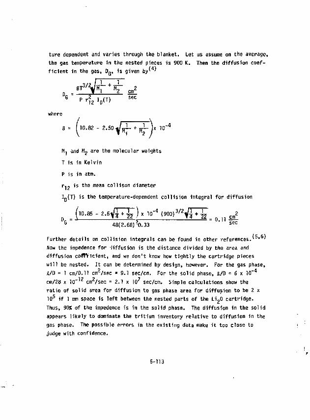
ture dependent and varies through the blanket. Let us assume on the average, the gas temperature in the nested pieces is 900 K. Then the diffusion coef­ficient in the gas, D G , is given by* '

= _J^[ZTcml G P rf 2 ID(T, « *

B T 3 ^

2.50

Mi and M 2 are the molecular weights T is in Kelvin P is in atm. r,? is the mean colli son diameter LJT) is the temperature-dependent collision integral for diffusion

D (l0-85 - 2.sVF¥) x !0-4 (900)^^7^ ^ cfZ G 48(2.68)?0.33 " s e c

Further details on collision integrals can be found in other references. * ' Now the impedence for liffusion is the distance divided by the area and diffusion coeTYicient, and we don't know how tightly the cartridge pieces will be nested. It can be determined by design, however. For the gas phase, 1/0 = 1 cm/0.11 cm2/sec = 9.1 sec/cm. For the solid phase, 1/0 = 6 x TO" 4

cm/28 x 10 cm2/sec = 2.1 x 10 7 sec/cm. Simple calculations show the ratio of solid area for diffusion to gas phase area for diffusion to be 2 x ID 5 if 1 mm space is left between the nested parts of the Li„0 cartridge. Thus, 90* of the impedence is in the solid phase. The diffusion in the solid appears likely to dominate the tritium inventory relative to diffusion in the gas phase. The possible errors in the existing data make it too close to judge with confidence.

5-113

Another factor needs to be considered, however. As the purge flow passes through the tube, the TjO content increases along both the external and internal traverse of the cartridge assembly. Consequently, there is a varying partial pressure throughout the tube, and it varies between tubes according to the generation rate and purge rate. The amount of LiOT dis­solved in the Li,0 depends on all these factors as well as the temperature of the Li 20, which varies within a given tube and also throughout the blanket depth.

Some work at ANL on determining the solubility experimentally was reported, but so far there are no results at our mean Li^O temperature of 900 K. This*could be one of the more significant effects influencing the total tritium inventory and deserves more study.

Using their lowest temperature data (1123 K), a rough calculation suggests an additional tritium inventory of ?.3 kg. Their data are not easy to extrapolate to lower temperatures, but the trend suggests the inventory would be lower at lower temperatures. Furthermore, by increasing the purge rate to 10" z of the bulk helium flow from the present value of 10 , the estimate above would drop to 230 g. This assumes that Henry's law is obeyed. That would keep the total blanket inventory below 1 kg even without taking advantage of the lower solubility expected at our temperatures.

5.4.3 Volatilization of LiQT

A question that has been raised in the past is that of volatilization of LiOT when it is in the presence of water vapor. This concern is quite valid, for we anticipate most of the tritium produced will be in the form of Tfl. The extent of volatilization and Li-0 loss can be seen to depend on both the temperature as well as the partial pressure of water vapor from the following equation' ':

l 0 9 PLiOH = " + 1 0 9 PH„0 + 5' 0 4 0)

5-114

where pressure is atm and temperature is Kelvin. The partial pressure of water vapor depends on the local breeding rate as well as the sweep rate of the helium purge gas through the tubes.

Referring to Section 5.4.7 on tritium processing and control, it may be seen that the flow is not uniform. The purge mass flow rate through the hottest, highest breeding rate zone is selected to be 100 times larger than through other parts of the breeding blanket. In the hottest part, the flow through each tube was therefore set at 3.85 x 10 ' g/sec. The volumetric flow rate is harder to work with for it increases constantly as the purge helium heats up as it passes through the tube. The breeding rate equals the evolution rate at steady state, so from the breeding rate equation, at the first wall where R = 152,

G = 3.13 x 1 0 1 5 exp(-4.35 x 10~ 2 R) * t o C T S

cm • sec and from the volume of lithium oxide in the tube

V = n(1.8 2 - 0.52)200 cm 3

15 the evolution rate is found to be 7.89 x 10 atoms/sec. Multiplying the flow rates by the appropriate factors, we can convert this information to that needed to calculate partial pressure.

.39 x 1 0 1 5 a t o m s " 9 H e

sec mole He 3.B5 x 10" 2 ||| 2 atoms 6.02 x 1 0 2 3 molecules

molecule mole 7 mole T ?0

If '.lis were a 1-atm system, the pressure would be very nearly 6.8 x 10 atm, but since it is a 48-atm system, the T 20 pressure is 3.27 x 10 atin. Inserting into Eq. (1),

109 "UOT = " TUJ + 1 o 9 ( 3 - 2 7 x 1°"5> + 5"04

5-115

where I have chosen the mean of the maximum Li,0 temperatures (on the inner diameter of the Li,0) within this high breeding rate zone of the submodule. The calculated pressure is PI.-QJ = 1.4 x 10 atm. The mass ratio of LiOT(g) to T-Ojg) is the molar (or partial pressure) ratio times appropriate molecular weight factors

1.4 x 10 7 .. 25 _ -'5 x "2? " 3.29 x 10 ° "

0.005 f ™

The mass flow rate of TgO is

7 89 x 1 0 1 5 a t 0 m s x m ? l f C U l e TJ0 * m ] e If 7 - 8 9 * 1 0 S T " * * atoms t * 6 > ( ? 2 x 10Xmlecules

22g T,0 , g T,0 mole T ?0 sec

So, the rate of LiOT loss is 0.005 x 1.44 x 10' 7 = 7.2 x 1 0 - 1 0 g/sec

This turns out to bo about 7 mg from this tube during a lifetime of three operating years. Deeper in the blanket, the breeding rates and temperatures are lower, which will reduce the volatility. Offsetting this partially is the purge flow rate that is reduced by a factor of 100. Nevertheless, it does not seem to pose a serious problem in this design.

5-116

5.5 NEUTRONICS

All of the neutronics calculations were performed with the one-dimensional code, ONEDANT. This is the most recent version of the discrete ordinates neutron transport code ONETIWP ' and includes the synthetic diffusion approximation

(9) developed by Alcouffe. ' The calculations were performed with S. quadrature and used 30 neutron groups coupled with 12 gamma groups to facilitate neutron transport and gamma ray production and transport. The group constants are of order P, and wer? obtained from the MATXS library by the TRANSX code.f 1 0' A similar translation produced the neutron and gamma kerna factors utilized in the heating edits. All of the cross section data are from the ENDF V files.

The initial blanket design was a helium cooled, lithium oxide design with Inconel structure. The initial design had excess breeding capacity, and neutronics work focused on lowering the breeding ratio and improving the overall blanket performance by placing additional structure in the breeding zone (see Table 5.13 ). The additional structure reduced the breeding ratio and increased the blanket energy multiplication, and also provided additional shielding for the superconductor coil. These results suggest that, in general, when excess tritium breeding is available, neutronics performance can be im­proved by adding structure beyond the amounts required for physical integrity.

Tritium recovery later became a primary concern, and led to the develop­ment of the blanket design described in Section 5.5.1. Neutronically, this design is similar to the previous designs, but contains a smaller Li 20 volume fraction, and correspondingly greater void and structural fractions. The work at this point focused on finding the best combination of breeding region thickness, Li^O volume fraction, and structure fraction that would satisfy all the requirements. Figures 5.37 and 5,38 show the results of some of this work. Details of this design are given in Table 5.14 and the results are presented in Table 5.15..

5-117

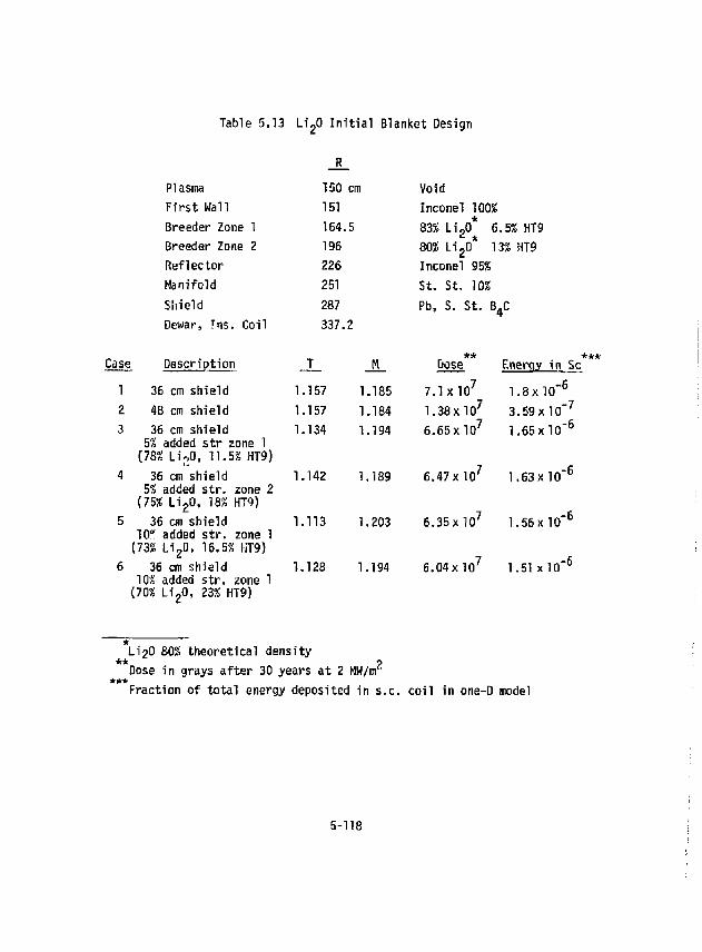
Table 5.13 L i -0 I n i t i a l Blanket Design

Plasma 150 cm Void First Wall 151 Inconel TOO? Breeder Zone 1 164.5 83% L i 2 0* 6.5% HT9 Breeder Zone 2 196 80% L i 2 0* 13% HT9 Reflector 226 Inconel 95? Manifold 251 St. St. 10% Shield 287 Pb, S. St. B4C Dewar, Tns. Coil 337.2

Case Description T M **

Dose Enerqy in Sc

1 36 cm shield 1.157 1.185 7.1 x l O 7 1 .8x l0 " 6

2 48 cm shield 1.157 1.184 1.38xl0 7 3.59 xlO""7

3 36 cm shield 5% added str zone 1

(78% LioO, 11.52 HT9)

1.134 1.194 6 .65x l0 7 1.65xl0" 6

36 cm shield 1.142 1.189 5% added s t r . zone 2

(75% L l 2 0 , 18% HT9) 36 cm shie ld 1.113 1.203

10" added s t r . zone 1 (73% L i 2 D , 16.5% HT9)

36 cm shie ld 1.128 1.194 10% added s t r . zone 1

(70% L i ' 2 0 , 23% HT9)

6 . 4 7 x l 0 7 1 .63X10" 6

6.35 x l O 7 1.56 x l O " 6

6 . 0 4 x l 0 7 1.51 x 1Q"6

LipO 80% theore t ica l densi ty * * o

Dose in grays a f te r 30 years a t 2 MW/m * * *

Fraction o f t o t a l energy deposited in s .c . c o i l i n one-D model

5-118

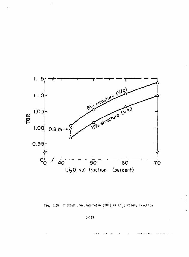
QD

0 .95 -

40 50 60 L i 2 0 vol. froction (percent)

70

Fiq. 5.37 Tritium breeding ratio (TBR) vs Li-0 volume fraction

6-119

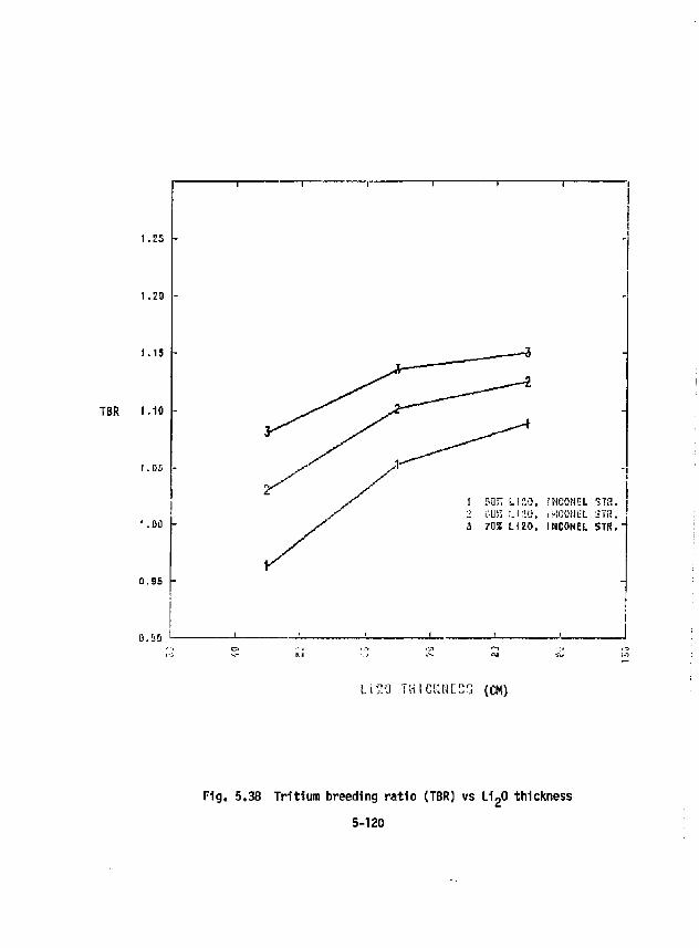
1.25

1.29

1.15

TBR 1.10

t.os

' .00

0.95

Q.fiO

1 ?as Lino, tne»ia •sra. 2 l-UK t .Ul i : . IMCfiWtL STB. 3 70% LIZO, IHCOHEL STR."

LI7.0 THICKNESS (CM)

Fig, 5.3B Tritium breeding rat io (TBR) vs LioO thickness

5-120

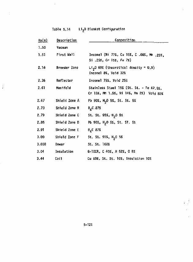
Table 5.14 LigO Blanket Configuration

Ro(m) Description Composition

1.50 Vacuum

1.51 First Wall Inconel (Ni 77%, Cu 15%, C .085',, Mh .25%, Si .25%, Cr 15%, Fe 11)

2.16 Breeder Zone Li«0 60? (theoretical density = 0,9)

Inconel 8%, Void 32%

2.36 Reflector Inconel 75%, Void 25%

2.61 Manifold Stainless Steel 1556 (St. St. - Fe 6>.5<&,

Cr 15%, Mn 1.5*, Ni 14%, Mn 2%) Void 85%

2.67 Shield Zone A Pb 90%, hy) 5%, St. St. 5%

2.73 Shield Zone B B4C87%

2.79 Shield Zone C St. St. 55%,-HgO 5%

2.85 Shield Zone D Pb 90%, H?0 5%, St. ST. 5%

2.91 Shield Zone E B4C 87%

3.00 Shield Zone F St. St. 95%, HgO 5%

3.038 Dewar St. St. 100%

3.04 Insulation G-10CR, C 40%, H 52%, 0 8%

3.44 Coil Cu 65%, St. St. 10%, Insulation 10%

5-121

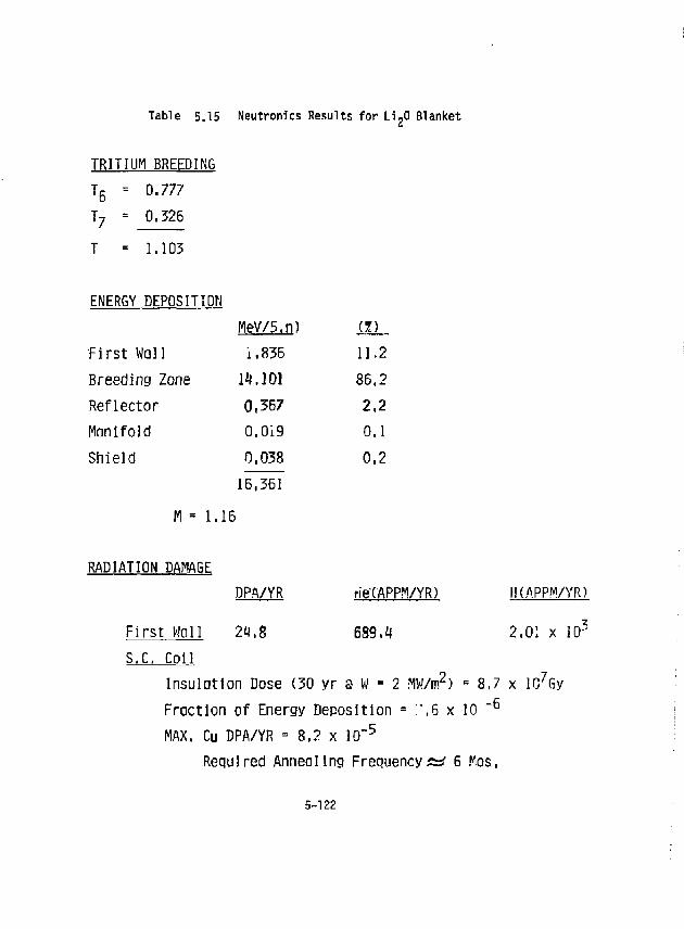
Table 5.15 Neutrom'cs Results for Li,0 Blanket

TRITIUM BREEDING T 5 = 0.777 T 7 = 0.326 T = 1.103

ENERGY DEPOSITION MeV/5,n) (Z)

First Wall i.836 11,2 Breeding Zone 14.101 86,2 Reflector 0,367 2,2 Manifold 0,019 0.1 Shield 0,038 0,2

16,361 M = 1.16

RADIATION DAMAGE

DPA/YR rie'CAPPM/YR) H(APPM/YR)

F i rs t Wall 2H.8 689.4 2.01 x 10 3

S.C, Col l

Insulation Dose (30 yr a W = 2 MW/m2) = 8,7 x 107Gy Fraction of Energy Deposition = :\6 x 10 " 6

MAX. Cu DPA/YR = 8.2 x 10~ 5

Required Annealing FrequencyzsJ 6 Mos,

5-122

Later in the project year it became apparent +tiat the use of Inconel as a structural material imposed significant penalties in neutronic performance. A systematic comparison of neutronic results was then performed for four structural materials:

(1) Inconel (2 1 Stainless steel (3) Tenelon (4) 2.25 Cr - 1 Mo These results are discussed in Section 5.5.4. Much of the work described

here is for the Initial Reference Blanket Design which includes Inconel structure. The final Reference Blunket Design, which is described in Section 5.5.4, is based on the use of Tenelon as the structural material. As shown below, '.he latter is a superior choice which offers the combination of better neutronic performance together with the needed materials characteristics.

Work has also begun on a low temperature, high breeding blanket. The axial-zoned high temperature blanket design described in Section 6.1 requires a low temperature blanket design with a breeding ratio of at least 1.4. The reference blanket design described in Section 5.5.1 does not provide adequate breeding for a two-axial-zone blanket concept as presently structured. How­ever, some very promising results have been obtained with a modification to this blanket design using a lead zirconate {Zr gPb 3) neutron multiplier. This design should be capable of producing high tritium breeding ratios (1.4 or greater) with enriched lithium oxide, or a tritium breeding ratio of 1.1 with approximately 20% of the blanket high temperature energy being deposited in a .iot shield as in a radially zoned blanket design. In the seconu option, the coola-it system would be split immediately after pass 3 through the breeding region, with the majority of the coolant bypassing the hot shield. The remaining coolant would pass through the hot shield and emerge at a substan­tially higher temperature.

The improved neutronic performance of the final reference blanket design may be sufficient to permit its use as the low temperature, high breeding blanket in an axial-zoned reactor without the presence of a neutron multiplier.

5-123

As described below in Section 5,5.4 the breeding ratio of this design can be fairly high for high volume fractions of Li"20. Depending on the Retails of the system integration, larger volume fractions might be acceptable in an axial-zoned reactor. In any event the improved neutronic results associated with the use of Teneion provides substantially greater design flexibility for both axial-and radial-zoned system, both with and without the use of a neutron multiplier.

5.5.1 Lithium Oxide initial Reference Blanket Design

The one dimensional representation of the reference LigO blanket is presented in Table 5.14. The breeding ratio has been homogenized, but this should not significantly affect the results.

The radial power density is shown in Figure 5.39. The power density is based on blanket volume rather than material volume. This particular design has a very high power density in the first wall, which is probahly due to a combination of the large amount of nickel in the Inconel structure, and the predominantly low Z material nearby.

Figure 5.40 shows the spatial distribution of the tritium breeding from both Lithium-6 and Lithtum-7. The small upturn at 210 cm is due to peaking off of the reflector. The Li-7 tritium production is exponential.

5.5.2 Radiation Damage

Radiation damage is an important consideration in any blanket design. Adequate shading is necessary to prevent damage to the superconducting coils, and to reduce the heat lead on the coil coolant system. Radiation damage to the first wall and blanket structure will cause a reduction in structural integrity. The most common means of measuring radiation damage are atomic displacements and gas production. Atomic displacements occur as a result of reactions with high energy neutrons. Atoms in a solid structure are displaced from their equilibrium lattice position, leaving a vacancy. Gas production occurs through both (n,p) and (n.alpha) reactions. Displacements are typically

5-124

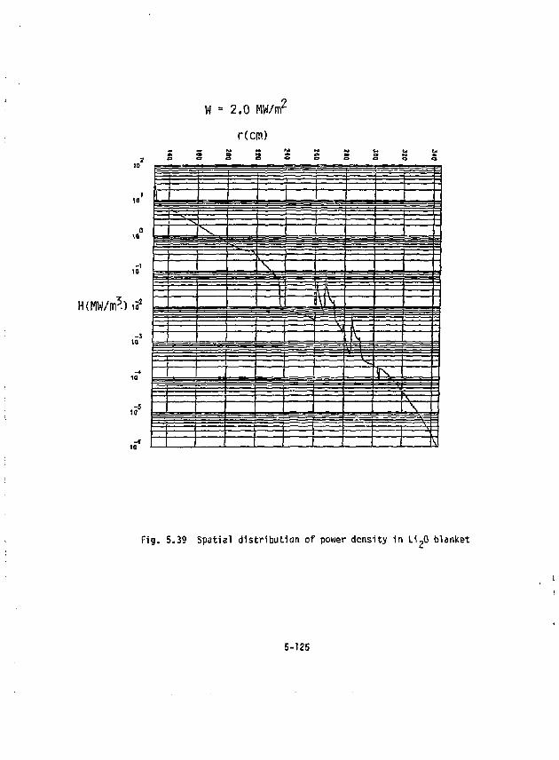
W • 2 . 0 MW/nf

r(OT) M f« Ftk N

0 Q

H(MW/m3-) i5 2

o o

1«

Fig. 5.39 Spatial distribution of power density in Li-0 blanket

5-125

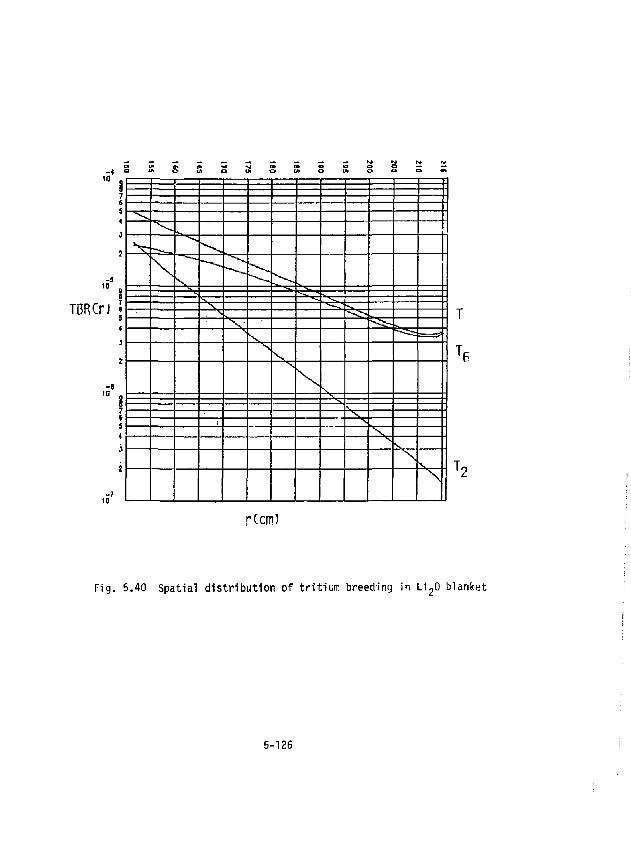
Q I f t O t / i a t f t O I S I Q Lh O CJi

4 nt

3 • *

1

"-V.

\ V

^ ^ V. "«-•> • O * ^ — V , v> v ** ^ N ^ • »

• •£

v

v V.

V s V \ v

\

r(cm)

Fig. 5.40 Spatial distr ibution of tr i t ium breeding in LijO blanket

5-126

reported in displacements per atom per year, and gas production in atom parts per million per year. All of these values are dependent upon the wall loading. Shielding requirements are generally determined by the radiation dose to the superconductor electrical insulation and by the displacements in the copper stabilizer. An additional consideration is the amount of energy deposited in the coil and dewar. Probably the most critical of these requirements is the superconductor insulation radiation dose. Current insulating materials are fairly radiation sensitive, and breakdown of the insulation would cause a failure of the coil. A widely used limit for the dose to the superconductor insulation is 5 x TO grays over the life time of the coil. Displacements in the copper stabilizer may not be as serious a problem if they can be annealed out with an acceptable cycle frequency.

In general, for every joule deposited in the superconducting coil ami dewar, 1000 joules are required to remove it. Because of this problem, an additional shielding requirement has been defined, namely, that the fraction of the total blanket energy deposited in +he superconducting coils and dewar be less than 10" , The amount of shielding required to meet this limit is usually sufficient to provide adequate protection of the superconducting coil insulation. The shield design used here is similar to the shield used in the WITAMIR report, consisting of alternating layers of lead, boron carbide, and steel.

Displacements and gas production rates have been computed by ONEDANT by taking constitutent edits and using displacement and gas production cross sections. The results of these calculations are shown in Figure 5.41, 5.42, and 5.43. A summary of this information is presented in Table 5.15.

5.5.3 ZrgPb3 Blanket

The use of a Zr 5Pb 3 as a neutron multiplier was first suggested in the STARFIRE study. The properties of ZfgPb 3 (Lead Zirconate) are mostly un­known, and its characteristics can only be imp'sied from information on other intermetalic compounds. The properties are generally considered to be

5-127

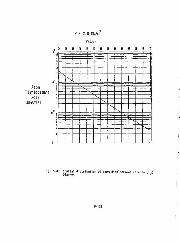
w - 2,0 i w r r(cra)

L* o » o *-»

Atom j Displacement ]

Rate J CDPA/YR)

- i ta

=4= — i — > — h i i

i i

i

V 1 x. K *-

^ ^

x \ ^

\ \ *s.

V V S k

Fig. 5.41 Spatial distribution of atom displacement rate in Li^O

5-128

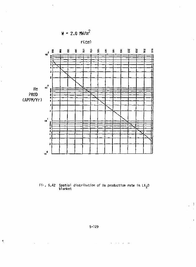
W • 2,0 HN/nf

r(cm)

hi M h»

He PROD

(APPM/Yr)

s — B»

r1—•**• t * a

T >•

T* t> a E» O LA a t*

t ^H— i 1 "* "*

5 V i i 1 v I

NL !

\ V

ft

N \

a , — J t = - X l ^

X V

IX V \ . s

i — i i — _ *v- ' j . *v.

s \ V

\

P i ' . 5.42 Spatial distribution of He production rate in Li~0 blanket c

5-129

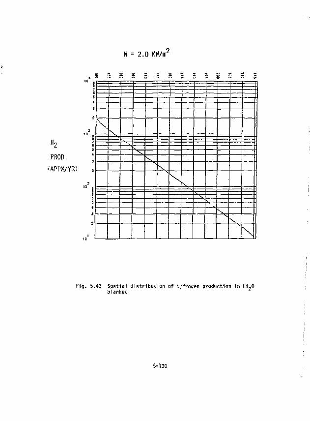
W = 2 . 0 HH/nr

K» N

H 2

PROD,

•APPH/YR)

t

1 a f L* • l * a •m a HI

r o a m t

1 1 I j 1 1

* 1 | • f

\ X -

« 'V

j. " N

, 1 -. J" V

' V "v

\ s, k =v-

3 *V \ s.

s \ X

N X

Fig. 5.43 Spatial d i s t r i b u t i o n of l\ -Voyen production in L i , 0 blanket i

5-130

attractive, particularly the high melting point (1400 C).

An initial design using a 19.5 cm Zr 5Pb, multiplier directly behind the first wall is shown schematically in Figure 5,44 This type of design has several advantages. The blanket energy miltiplication is much higher than a non-multiplier design. Also, the breeding region can be relatively thick with fairly uniform lithium burnup (Figure 5.45). The multiplier also provides an additional benefit. The high Z multiplier material near the first wall acts as a shield to gammas generated internally in the Blanket. This results in a significant reduction in the energy deposition in the first wall.

Additional work on this design indicates that a breeding ratio of 1.1 can be obtained with a 10 on multiplier region and a 10 cm breeding zone with 60% Li-6 enrichment. There are any number of combinations of multiplier thick­ness and breeding zone thickness that will provide a tritium breeding ratio of 1.1, with the general trend of increasing M value with increasing multiplier thickness (Figure 5.46). In all cases, at a T value of 1,1 the amount of energy deposited in the hot shield is approximately 25%.

This particular blanket design can also achieve very high breeding ratios by increasing the Li,0 thickness. A breeding ratio greater than 1.4 is quite possible. This one blanket design has the flexibility, therefore, to be adapted to either a radially zoned design, or an axially zoned design.

5.5,4 Blanket Structure

The initial reference low temperature blanket design achieves a breeding ratio that 1s only barely adequate despite the fact that it contains a large amount of MoO. The reason for this poor neutronic performance was previously thought to be due ty the high structure fraction 1n the breeding zone. But a comparison with a similar design using different structural materials indicated thai the problem was due more to the type of structure rather than the amount of structural material used.

5-131

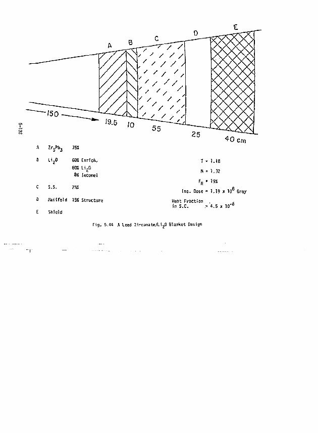
40 cm A Zr5Pb3 752

0 u2o 60X £nrich. 60% LijO 8% Inconel

C S.S. 75%

0 Manifold 1555 Structure

E Shield

Fig. 5.14 ft Lead Zirconate/LijO Blanket Design

T « 1.18 M = 1,32 F„ = 1 M

Ins. Dose = 1.19 x 10 Gray Heat Fraction in S.C. 4.5 x 10'

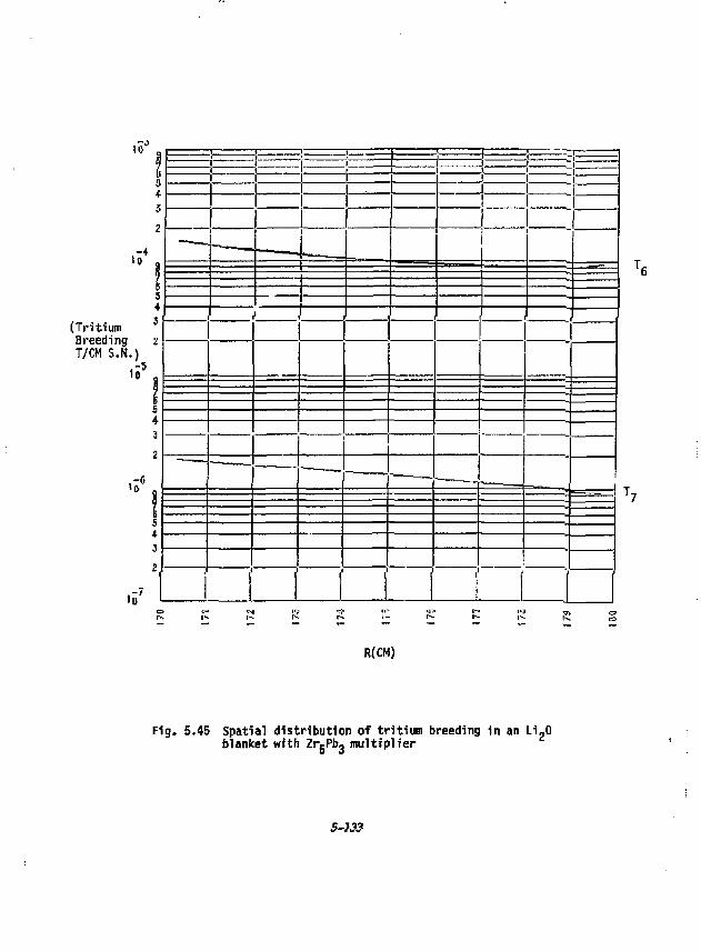
10

to

(Tritium Breeding T/CM S.N.)

i iS 5

rf

-7 ID

R(CM)

Fig. 5.45 Spatial distribution of t r i t ium breeding in an Li-0 blanket with ZrgPb3 mult ipl ier

3-739

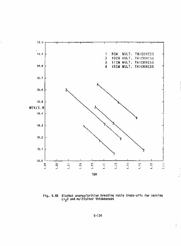
i».1 -

1 BCM MULT. THICKNESS 2 10CM MULT. THICKNESS o 11 CM MULT. THICKNESS 4 1SCM MULT. THICKNESS

TBR

Fig. 5.46 Blanket energy/tritium breeding ratio trade-offs for varying LipO and multiplier thicknesses

5-134

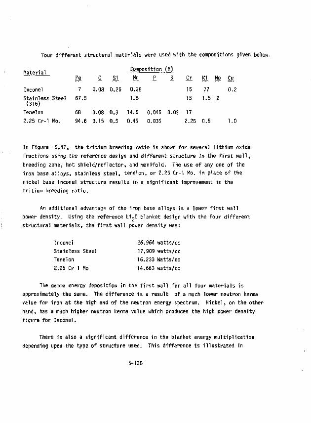
Four different structural materials were used with the compositions given below.

Material Fe C Si Composition Kn P

m s Or Ni Mo Cu

Inconel 7 0.08 0.25 0.25 15 77 0.2 Stainless Steel (316)

57.5 1.5 15 1.5 2

Tenelon 68 0.08 0.3 14.5 0.045 0.03 17 2.25 Cr-1 Mo. 94.6 0.15 0.5 0.45 0.035 2.25 0.5 1.0

In Figure 5.47, the tritium breeding ratio is shown for several lithium oxide fractions using the reference design and different structure in the first wall, breeding zone, hot shield/reflector, and manifold. The use of any one of the iron base alloys, stainless steel, tenelon, or 2.25 Cr-1 Mo. in place of the nickel base Inconel structure results in a significant improvement in the tritium breeding ratio.

An additional advantage of the iron base alloys is a lower first wall power density. Using the reference Li^O blanket design with the four different structural materials, the first wall power density was:

Inconel 26.964 watts/cc Stainless Steel 17.909 watts/cc Tenelon 16.233 Watts/cc 2.25 Cr 1 Mo 14.663 watts/cc

The gamma energy deposition in the first wall for all four materials is approximately the same. The difference is a result of a much lower neutron kerma value for iron at the high end of the neutron energy spectrum. Nickel, on the other hand, has a much higher neutron kerma value which produces the high power density figure for Inconel.

There is also a significant difference in the blanket energy multiplication depending upon the type of structure used. This difference is illustrated in

5-135

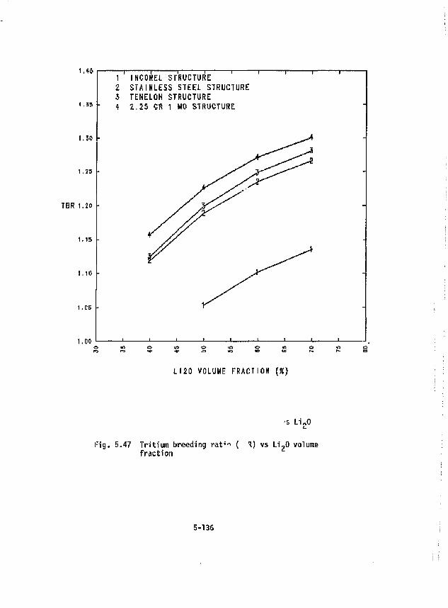
l.tft i i 1 1 1 1 1 1 1 r 1 INCOHEL S T R U C T U R E 2 STAINLESS STEEL STRUCTURE i TENELON STRUCTURE

' " - 4 1.25 CR 1 MO STRUCTURE

1.3* r

1.25 -

TBR 1.20 -

1.15 -

1.10 -

1.05 -

1. po ' ' ' ' ' ' ' ' ' ' '. n r s - * - - 4 ' W i r a » a j i w r ~ m

L I20 VOLUME FRACTION (%}

'S LioO L.

Fig. 5.47 Tritium breeding rat**1 ( 1) vs Li^O volume fraction

5-136

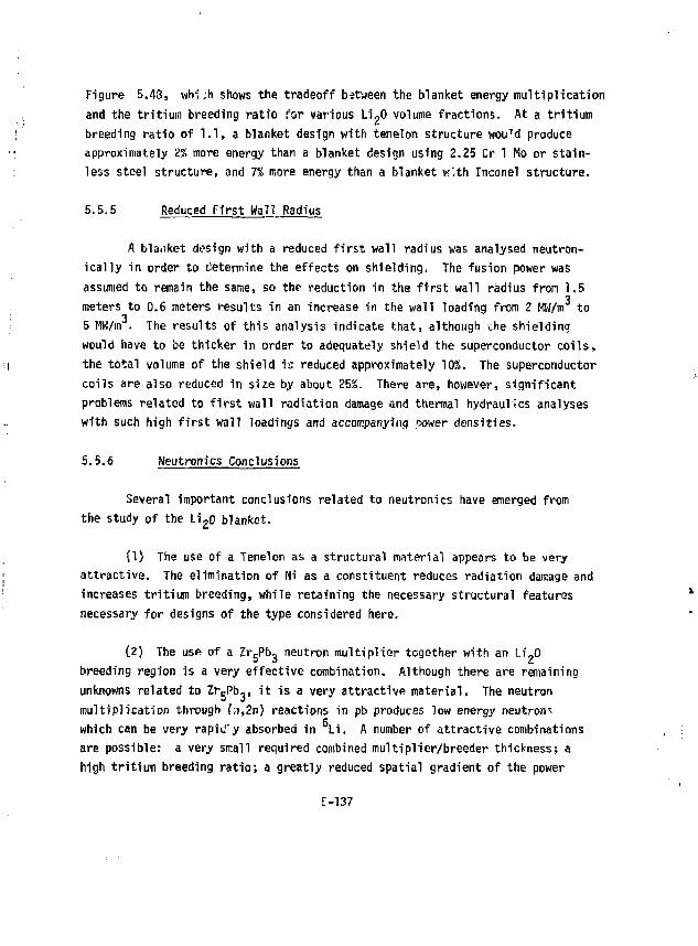
Figure 5.43, whi ;h shows the tradeoff between the blanket energy multiplication and the tritium breeding ratio r'or various LigO volume fractions. At a tritium breeding ratio of 1.1, a blanket design with tenelon structure wou 7d produce approximately It more energy than a blanket design using 2.25 Cr 1 Mo or stain­less steel structure, and 7% more energy than a blanket v;!th Inconel structure.

5.5.5 Reduced First Wall Radius

A blanket dosign with a reduced first wall radius was analysed neutron-ically in order to determine the effects on shielding. The fusion power was assumed to remain the same, so the reduction in the first wall radius from 1.5 meters to 0.6 meters results in an increase in the wall loading from 2 MW/m to

3 5 MW/m . The results of this analysis indicate that, although che shielding would have to be thicker in order to adequately shield the superconductor coils, the total volume of the shield is reduced approximately 102S. The superconductor coils are also reduced in size by about 25%. There are, however, significant problems related to first wall radiation damage and thermal hydraulIcs analyses with such high first wall loadings and accompanying sower densities.

5.5.6 Neutrom'cs Conclusions

Several important conclusions related to neutronics have emerged from the study of the Li 2o blanket.

(1) The use of a Tenelon as a structural material appears to be very attractive. The elimination of Ni as a constituent reduces radiation damage and increases tritium breeding, whiTe retaining the necessary structural features necessary for designs of the type considered here.

(2) The use of a Zr gPb 3 neutron multiplier together with an Li' 0 breeding region is a very effective combination. Although there are remaining unknowns related to ZrgPb,, it is a very attractive material. The neutron multiplication through (;i,2n) reactions in pb produces low energy neutron-which can be very rapic"y absorbed in Li. A number of attractive combinations are possible: a very small required combined multiplier/breeder thickness; a high tritium breeding ratio; a greatly reduced spatial gradient of the power

£-137

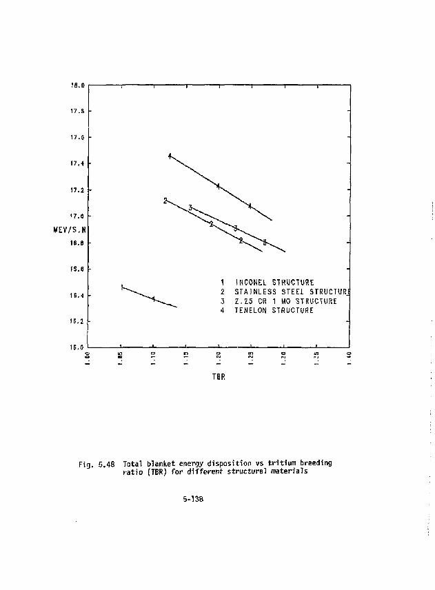
1 INCONEL STRUCTURE 2 STAINLESS STEEL STRUCTURJ 3 2,15 CR 1 MO STRUCTURE 4 TENELON STRUCTURE

TBR

Fig. 5.48 Total blanket energy disposition vs t r i t ium breeding rat io (TBR) for different structural materials

5-138

density; a relatively high percentage of energy deposited in the hot shield (with a constr . of T>.1,1).

(3) The power density in the first wall of a typical blanket design is significantly impacted by the type of material used in the adjacent region. The use of a high Z material, such as Zr 5Pb 3 or LiPb for example, causes gamma ray absorption to be concentrated there rather than in the first wall. This reduces the first wall power density and makes its design less difficult.

5-139

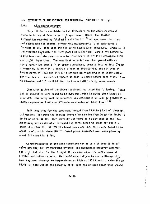
5.6 ESTIMATION OF THE PHYSICAL AND MECHANICAL PROPERTIES OF LIgO 5.6.1 Li„0 Microstructure

Very little is available in the literature on the microstructural characteristics of fabricated Li„0 specimens. Hence, the limited

(12) information reported by Takahashi and Kikuchv ' on specimens that they had fabricated for thermal diffusivity measurements is of considerable interest to us. They used the following fabrication procedure. Granules of the starting LioO material (designated as CERAC/PURE) were first heated in a platinum crucible under vacuum for four hours at 973 K to decompose L10H and li'CO, impurities. The resultant material was then ground with an agate mortar and pestle in an argon atmosphere, pressed into pellets (10 mm diameter by 13 mm high) without a binder at 100-500 ^Pa, and sintered at temperatures of 1373 and 1473 K in covered pla+lnum crucibles under vacuum for four hours. Specimens prepared in this way were sliced into discs lo mm in diameter and 1,3 mm thick for the thermal diffusivity measurements.

Characterization of the above specimens indicated the following. Total cation impurities were found to be 0.05 wt%, with Ca being the highest a.t 0.02 wt%. The x-ray lattice parameter was determined as 0.46117 ± 0.00Q05 nm which compares well with an NBS reference value of 0.46114 nm. '

Bulk densities for the specimens ranged from 70.8 to 93.4% of theoreti­cal density (TD) with the average grain size ranging from 20 um for 70.$% TD to 60 ^, at 93.4% TD. Open porosity was found to be dominant at the lower densities, but as density increased the pores began to close off rapidly abovs about 86% TD. At 88% TD-closed pores and open pores were found to be about equal, while above 90% TD closed pores dominated over open pores by about 5:1 (see Fig. 5.49).

An understanding of the pore structure variation with density is of valu§ not only for interpreting physical and mechanical property behavior for Li 0, but also for the insight it can give us on the mechansisms of trittum and helium release. We should especially note that although Li 20 that has been sintered to temperatures as high as 1473 K and to a density of 93.4SJ TD, some 20% of the porosity still consists of open pores that should

5-14&

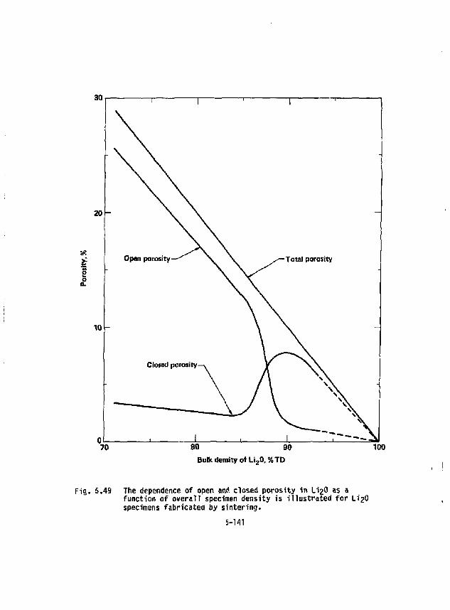
70 80 90 100 Bulk density of Li z0, %TD

Fig. 5.49 The dependence of open and closed porosity in U2O as a function of overall specimen density is i l lustrated for LigO specimens fabricated by sintering.

5-141

provide a network of passages throughout, the structure for release of tritium and helium.

5.6.2 Thermal Conductivity

Using the methods of specimen preparation described above, Takahashi and Kikuchv ^' measured thermal diffusivities of Li ?0 in the range of 70.8 to 1'iA% TD and temperatures of 473 to 1173 K. Thermal conductivities were then calculated from the thermal diffusivity values using literature information on specific heat and density to make the calculation. The data thus derived are summarized in Fig. 5.50, which also shows an extrapolation to 100* TD using the Maxwell-Eucken equation to make the extrapolation. The analytical expression used by Takahashi and Kikuchi to fit their data is slightly modified here to express it in terms of volume fraction porosity (instead of fraction of theoretical density) as follows:

k = (1 - p ) 1 * 9 4 (0.0?<tf + 1.784 x 10" 4 T)"' (5.331

5.6.3 Thermal Expans'vity

Kurasawa' ' has recently measured the percent thermal expansion up to "V1200 K for both single crystal and sintered specimens of Li" 0 using a dilatometer to make the measurements. Two single crystal specimens, prepared from molten Li„0 by a floating zone technique, were used. Each specimen was 8 mm in diameter by 88 mm long. Five sintered specimens were prepared for the measurements using the method described by Takahashi and Kikuchv ' {see above). The sintered specimens were in the form of bars 4 x 4 x 10 mm, and had densities of 75.5, 80.0, 86.7, and 92.5% TD.

Kurasawa's measurements on the single crystals showed a fair degree of variability between runs, especially at the higher temperatures. For example, the percent linear expansion from room temperature to 1173 K ranged from 2.47 to 2.82% for five different runs, which gives a spread of ± 6.6% aDOut the mean. For each individual run, however, the standard deviation about a fitted curve for that run was quite good, being about 1-2%. Individual data points are not given for the sintered samples, but standard

5-142

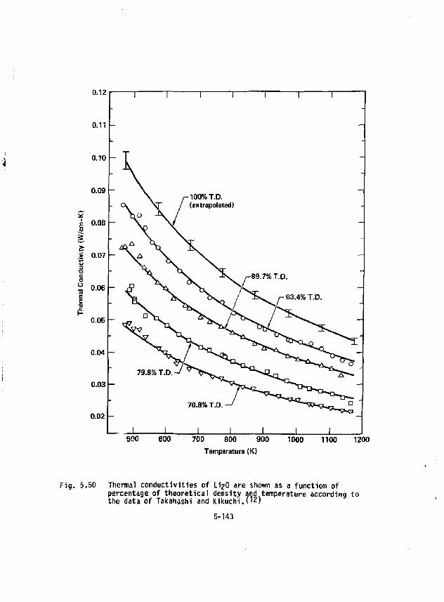
0.12

700 800 900 Temperature (K)

1000 1100 1200

Fig. 5.50 Thermal conductivities of LigO are shown as a function of percentage of theoretical densit. the data of Takahashi and Kikuch percentage of theoretical density arid temperature according to 1.(12)

5-143

deviations are indicated to be of the order of \% about the fitted curves. Agreement appears to be good for percent thermal expanfion from room temperature up to about 110u K for the averaged singla crystal data and the sintered samples. Above 1100 K, the percent expansion curve shows a drop-off in slope with increasing temperature for samples with 80.0, 86.7, and 91.1% TD, but a normal continuation of the curves for 75.5, 92.5, and 100.OK TO.

In order to obtain thermal expansivity values from Kurasawa's data, we need to differentiate the fractional expansion curves. We have a problem in dointj this because of the variations in the data, especially at high temperatures. Therefore, our approach is to fit an average curve to the data up to 1100 K, and then allow the curve to rise in a normal manner above tnat temperature. The functional form of the curve is taken to be one that has previously been shown to be applicable to a large number of substances, including metals, oxides, borides, carbides, and nitrides.^ ' Thus, the averaged expression for fractional linear expansion,AL/L, and the derived linear thermal expansivity, a, are found to be as follows:

dL/L 0 = - 4.275 x 10" 3 + 1.4692 x 10" 6 T 1 ' 4 (5.34)

a = d(dL/L0)/dT = 2.0569 x 10" 6 T 0 - 4 , K" 1 (5.35)

Fractional linear expansions calculated using equation (5.34) are compared in Table 5.16 with the averaged single crystal data and the 92.5% TD sintered data given by Kurasawa.^ ' The linear thermal expansivity obtained from equation (5.35) is also summarized in Table 5.16.

5-6.4 Mechanical Properties

Experimental information on the mechanical properties of Li'oO is totally lacking at the present time. We must therefore rely on correlations based on other oxides to obtain some rough values with which to proceed with design calculations. Some theoretical guidance is also available in regard to variation of mechanical properties with grain size and specimen porosity. The main design need for mechanical properties for Li-G is to

5-144

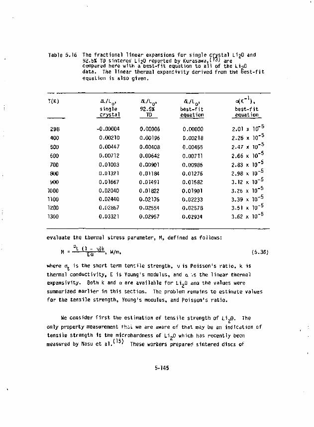
Table 5.16 The fractional linear expansions for single crystal LigO and 92.5% TO sintered LigO reported by Kurasawa,('3) are compared here with a best-fit equation to all of the Li?0 data. The linear thermal expansivity derived from the best-fit equation is also given.

T(K) fl./L„. single crystal

-0.00004

a/L0, 92.5*

TD

0.00006

best-fit equation

0.00000

best-fit equation

298

fl./L„. single crystal

-0.00004

a/L0, 92.5*

TD

0.00006

best-fit equation

0.00000 2.01 x 10" 5

400 0.00210 0.00196 0.00218 2.26 x 10" 5

500 0.00447 0.00408 0.00455 2.47 x 10" 5

600 0.00712 0.00642 0.00711 2.66 x 10" 5

700 0.01003 0.00901 0.00986 2.83 x 10" 5

800 0.01321 0.01184 0.01276 2.98 x 10" 5

900 0.01667 0.01491 0.01582 3.12 x 10' 5

100C 0.02040 0.01822 0.01901 3.26 x 10" 5

1100 0.02440 0.02176 0.02233 3.39 x 10" 5

1200 O.t'2867 0.02554 0.02578 3-51 x 10" 5

1300 0.03321 0.02957 0.02934 3.62 x 10" 5

evaluate the thermal stress parameter, M, defined as follows:

Ea -, W/m, (5.36)

where o t is the short term tensile strength, v> is Poisson's ratio, k is thermal conductivity, E is Young's modulus, and a .s the linear thermal expansivity. Both k and a are available for Li«0 and the values were summarized earlier in this section. The problem remains to estimate values for the tensile strength, Young's modulus, and Poisson's ratio.

We consider first the estimation of tensile strength of Li_0. The only property measurement thii. we are aware of that may be an indication of tensile strength is the microhardness of Li~0 which has recently been measured by Nasu et al. (15) These workers prepared sintered discs of

5-145

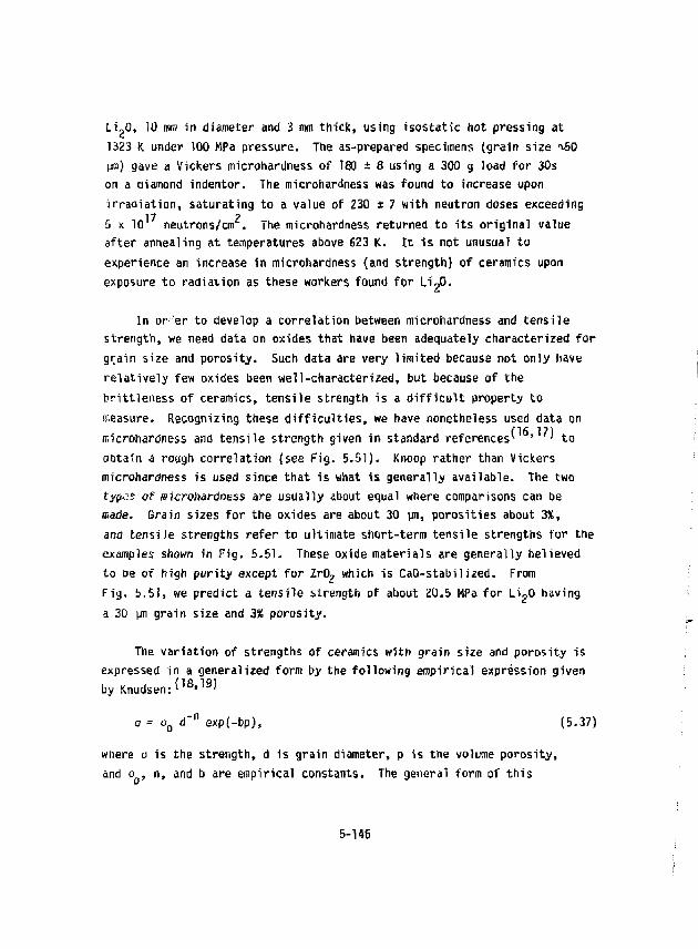
li ?0, 10 mm in diameter and 3 mm thick, using isostatic hot pressing at 1323 K under 100 MPa pressure. The as-prepared specimens (grain size ^60 \M) gave a Vickers microhardness of 180 ± 8 using a 300 g load for 30s on a diamond indentor. The microhardness was found to increase upon irradiation, saturating to a value of 230 s 7 with neutron doses exceeding

17 2 5 x 10 neutrons/cm . The microhardness returned to its original value after annealing at temperatures above 623 K. It is not unusual to experience an increase in microhardness (and strength) of ceramics upon exposure to radiation as these workers found for LioO.

In or'er to develop a correlation between microhardness and tensile strength, we need data on oxides that have been adequately characterized for grain size anil porosity. Such data are very limited because not only have relatively few oxides been well-characterized, but because of the brittleness of ceramics, tensile strength is a difficult property to measure. Recognizing these difficulties, we have nonetheless used data on fflicrohardness and tensile strength given in standard references^ J ' to obtain a rough correlation (see Fig. 5.51). Knoop rather than vickers microhardness is used since that is what is generally available. The two ty{k?s of microhardness are usually about equal where comparisons can be made. Grain sizes for the oxides are about 30 un, porosities about 3%, and tensile strengths refer to ultimate short-term tensile strengths for the examples shown in Fig. 5.51. These oxide materials are generally believed to be of high purity except for Zr0 2 which is CaQ-stabilized. From Fig. 5.51, we predict a tensile strength of about 20.5 MPa for Li^O having a 30 UTI grain size and 3% porosity.

The variation of strengths of ceramics with grain size and porosity is expressed in a generalized form by the following empirical expression given by Knudsen:* 1 8' 1 9*

<7= a Q d' n exp(-bp), (5.37)

wiiere o is the strength, d is grain diameter, p is the volume porosity, and o , n, and b are empirical constants. The general form of this

5-146

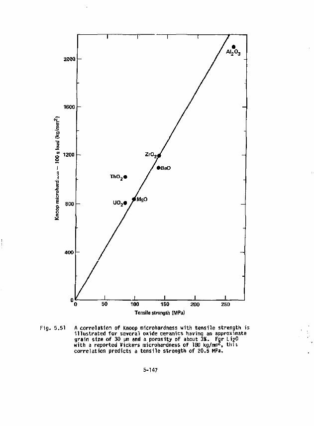
2000

1600 -

i I

1200

800

400 -

100 150 Tensile strength (MPa)

200 250

Fig. 5.51 A correlation of Knoop microhardness with tensile strength is illustrated for several oxide ceramics having an approximate grain size of 30 \m and a porosity of about 3%. For LigO with a reported Vickers microhardness of 180 kg/mmz, this correlation predicts a tensile strength of 20.5 MPa.

5-147

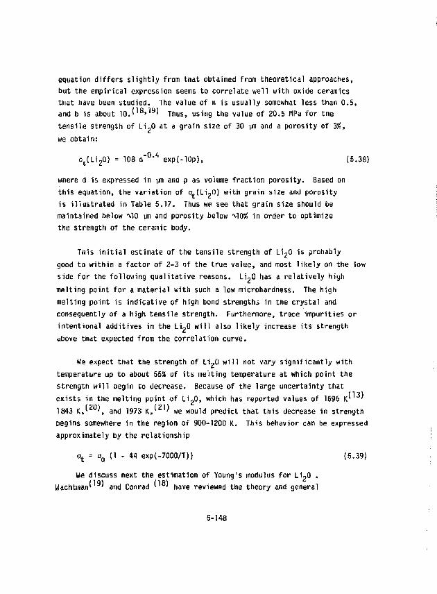
equation differs slightly from that obtained from theoretical approaches, but the empirical expression seems to correlate well with oxide ceramics that have been studied. The value of n is usually somewhat less than 0.5, and b is about 10.( 1 8> 1 9) Thus, using the value of 20.5 MPa for tne tensile strength of Li ?0 at a grain size of 30 \rt\ and a porosity of 2%, we obtain:

o t(Li 20) = 108 d ~ 0 - 4 exp(-lOp), (5.38)

wnere d is expressed in \m and p as volume fraction porosity. Based on this equation, the variation of a(Li 20) with grain size and porosity is illustrated in Table 5.17. Thus we see that grain size should be maintained below V|o un and porosity below ^\Q% in order to optimize the strength of the ceramic body.

This initial estimate of the tensile strength of Li^O is probably good to within a factor of 2-3 of the true value, and most likely on the low side for the following qualitative reasons. Li-0 has a relatively high melting point for a material with such a low microhardness. The high melting point is indicative of high bond strengths in the crystal and consequently of a high tensile strength. Furthermore, trace impurities or intentional additives in the LioO will also likely increase its strength above that expected from the correlation curve.

We expect that the strength of LioO will not vary significantly with temperature up to about 55% of its melting temperature at which point the strength will begin to decrease. Because of the large uncertainty that

(131 exists in the melting point of Li-0, which has reported values of 1695 Kv ' 1843 K J Z 0 \ and 1973 K,^ 2 1^ we would predict that this decrease in strength begins somewhere in the region of 900-1200 K. This behavior can be expressed approximately by the relationship

o t = o 0 (1 - 44 exp(-7000/T)) (5.39)

We discuss next the estimation of Young's modulus for Li«0 . Wachtman* ' and Conrad ^'"' have reviewed the theory and general

5-148

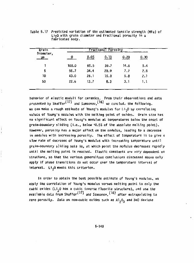
Table 5.17 Predicted variation of the estimated tensile strength (MPa) of LigO with grain diameter and fractional porosity in a fabricated body.

Grain Fractional Poros i t y Diameter,

0 0.05 0.10 0.20 0.30

1 108.0 65.5 39.7 14.6 5.4 5 56.7 34.4 20.9 7.7 2.8

10 43.0 26.1 15.8 5.8 2.1 50 22.6 13.7 8.3 3.1 1.1

behavior of elastic moduli for ceramics. From their observations and data presented by Shaffer^ ' and Samsonov,' ' we conclude the following. We can make a rough estimate of Young's modulus for Li,0 by correlating values of Young's modulus with the melting point of oxides. Grain size has no significant effect on Young's modulus at temperatures below the onset of grain-boundary sliding (i.e., below "V).55 of the absolute melting point). However, porosity has a major effect on the modulus, leading to a decrease in modulus with increasing porosity. The effect of temperature is to give a slow rate of decrease of Young's modulus with increasing temperature until grain-boundary sliding sets in, at which point the modulus decreases rapidly until the melting point is reached. Elastic constants are very dependent on structure, so that the various generalized conclusions discussed above only apply if phase transitions do not occur over the temperature interval of interest. Li ?0 meets this criterion.

In order to obtain the best possible estimate of Young's modulus, we apply the correlation of Young's modulus versus melting point to only the cubic oxides (Li-0 has a cubic inverse fluorite structure), i>nd use the available data from Shaffer' 1 7' and Samsonov,' ' after extrapolating to zero porosity. Data on non-cubic oxides such as Al„0, and BeQ deviate

5-149

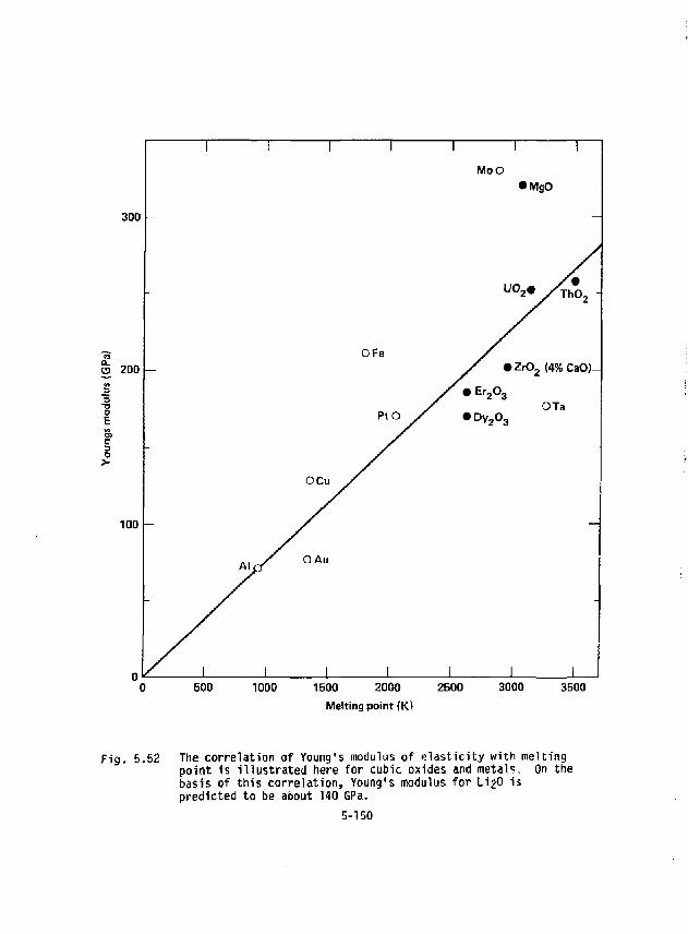
I I I I I I I MoO

• MgO

300

_ U ° 2 » / T h 0 2 -

"eo OFe O 200 / • Z r 0 2 ( 4 % C a O ) -

.3 "5 o E

PtO / / • E r 2 ° 3

f OTa • D y 2 0 3

Youn

gs

OCu

-

100

AlrT OAu

-

_L 500 1000 1500 2000

Melting point (Kl 2500 3000 3500

Fig. 5.52 The correlation of Young's modulus of elasticity with melting point is illustrated here for cubic oxides and metals. On the basis of this correlation, Young's modulus for LijO is predicted to be about 140 GPa.

5-150

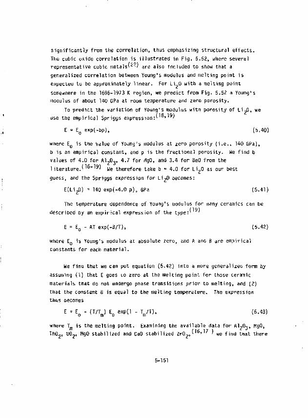
significantly from the correlation, thus emphasizing structural effects. The cubic oxide correlation is illustrated in Fig. 5.52, where several representative cubic metals'^' are also included to show that a generalized correlation between Young's modulus and melting point is expected to be approximately linear. For Li 0 with a welting point somewhere in the 1696-1973 K region, we predict from Fig. 5.52 a Young's modulus of about 140 GPa at room temperature and zero porosity.

To predict the variation of Young's modulus with porosity of Li,0, we use the empirical Spriggs expression:1 ' '

E = E Q exp(-bp), (5.40)

where E is the value of Young's modulus at zero porosity (i.e., 140 GPa), b is an empirical constant, and p is the fractional porosity. We find b values of 4.0 for A1 20 3, 4.7 for MgO, and 3.4 for BeO from the literature.' 1 6" 1 9) w e therefore take b = 4.0 for LigO as our best guess, and the Spriggs expression for LigO becomes:

E(Li20) = 140 exp(-4.0 p), GPa (5.41)

The temperature dependence of Young's modulus for many ceramics can be described by an empirical expression of the type:v '

E = E 0 - AT exp(-B/T), (5.42)

where E Q is Young's modulus at absolute zero, and A and B are empirical constants for each material.

We finu that we can put equation (5.42) into a more generalized form by assuming (1) that E goes to zero at the melting point for those ceramic materials that do not undergo pnase transitions prior to melting, and (2) that the constant 8 is equal to the melting temperature. The expression thus becomes

E = E Q - (T/Tj E Q exp(l - Jjl), (5.43)

where T_ is the melting point. Examining the available data for Al,0 3, MgO, ThQ z, U0 2, MgO stabilized and CaO stabilized Z r O ^ ^ 1 6 ' 1 7 ) we find that there

5-151

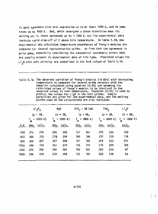
is good agreement with this expression up to at least 1200 K, and in some cases up to 1800 K, BeO, which undergoes a phase transition near its melting po! t, shows agreement up to -v 1300 K, but the experimental data indicate rapid drop-off of E above this temperature. In Table 5.18, the experimental and calculated temperature dependences of Young's modulus are compared for several representative oxides. We find that the agreement is quite gooo, expecially considering the substantial systematic errors that are usually present in experimental data of this type. Predicted values for Li p0 with zero porosity are summarized in the last column of Table 5.18.

Table 5.18 The observed variation of Young's modulus (in GPa) with increasing temperature is compared for several oxide ceramics with the behavior calculated using equation (5.43) and assuming the calculated values of Young's modulus to be identical to the observed values at room temperature. Equation (5.43) is used to predict the values for l_i?0 in the last column. Sample porosities are given for the experimental data, and the melting points used in the calculations are also indicated.

A' i 2o 3 MgO ZrO ? • • +X CaO ThO ? Li 20

(P = 2%, (P = 2%, (P = 4St, (P = 3%, (P = 03 T = m 2320 K) T = m 2850 K) T =

m 3000 K) T =

m 3490 K) T = 185C m

T,K obs. calc. obs. calc. obs. calc. obs. calc. calc.

298 376 376 295 295 167 167 235 235 140 600 366 370 278 294 164 166 231 235 134 800 356 357 267 289 161 164 224 233 124 1000 344 333 257 279 155 159 216 229 108 1200 324 300 246 264 149 152 209 223 87 1400 294 258 234 244 122 142 200 214 63

5-152

Finally, we need to estimate Poisson's ratio for Li,0- When a specimen is loaded in tension, there occurs a decrease in thickness along with the increase in length. The ratio of this decrease in thickness to increase in length is called Poisson's ratio and is given by

Poisson's ratio is also related to Young's modulus and the shear modulus by the following equation:

v ^ - l (5.45}

Poisson's ratio for most materials, including ceramics, generally is between 0.15 and 0.4.

To a first approximation, Poisson's ratio should be independent of specimen porosity and temperature since both Young's modi'lus and the shear modulus show nearly the same porosity and temperature dependence. There are minor differences, however, and we especially might expect an increase in v at high temperatures when grain boundary sliding becomes important {e.g., see Fig. 5.63). Small amounts of chemical additives may also influence Poisson's ratio. For example ThO., that contains 0.5% CaO exhibits a Poisson's ratio of twice that of pure Th0 2 (see Fig. 5.53).

It is difficult to make an accurate estimate of Poisson's ratio for Li ?0. Wide variations are seen in the reported data for even conventional ceramic materials such as Al-O, and HgO* 6' 1 7' 2 3^ (see Fig. 5.53). We therefore choose to take roughly a mean value, based on all materials, of v = 0.25 for Li^O, and further assume that v is independent of porosity, temperature, and chemical purity. The uncertainty in this value could be as much a factor of two.

5,6.5 Thermal Stress Parameter

We are now in a position to calculate values of the thermal stress parameter M for Li^O as defined in equation (5.36). Analytical

5-153

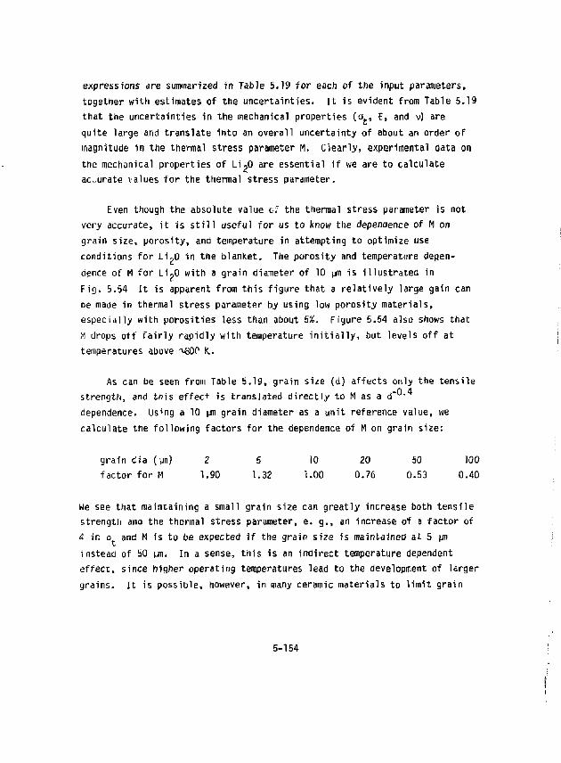
expressions are summarized in Table S.19 for each of the input parameters, together with estimates of the uncertainties. It is evident from Table 5.19 that the uncertainties in the mechanical properties (o , E, and v) are quite large and translate into an overall uncertainty of about an order of magnitude in the thermal stress parameter M. Clearly, experimental data on the mechanical properties of Li,0 are essential if we are to calculate accurate values for the thermal stress parameter.

Even though the absolute value of the thermal stress parameter is not very accurate, it is still useful for us to know the dependence of M on grain size, porosity, and temperature in attempting to optimize use conditions for Li~0 in the blanket. The porosity and temperature depen­dence of M for Li ?0 with a grain diameter of 10 yn is illustrated in Fig. 5.54 It is apparent from this figure that a relatively large gain can De made in thermal stress parameter by using low porosity materials, especially with porosities less than about 5%. Figure 5.54 also shows that M drops off fairly rapidly with temperature initially, but levels off at temperatures above ^W0 K.

As can be seen from Table 5.19, grain size (d) affects only the tensile strength, and tnis effect j s translated directly to M as a d" 0 -

dependence. Us^ng a 10 urn grain diameter as a unit reference value, we calculate the following factors for the dependence of M on grain size:

grain dia (un) 2 5 10 20 50 100 factor for M 1.90 1.32 1.00 0.76 0.53 0.40

We see that maintaining a small grain size can greatly increase both tensile strength and the thermal stress parameter, e. g., an increase of a factor of 4 in o, and M is to be expected if the grain size is maintained at 5 ur> instead of SO urn. In a sense, this is an indirect temperature dependent effect, since higher operating temperatures lead to the development of larger grains. It is possible, however, in many ceramic materials to limit grain

5-154

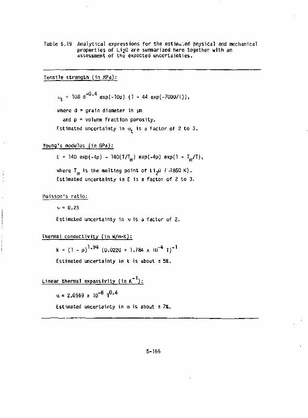
Table 5.19 Analytical expressions for the estimated physical and mechanical properties of LigO are summarized here together with an assessment of the expected uncertainties.

Tensile strength (in MPa):

o t = 108 d ~ 0 , 4 exp(-lOp) (1 - 44 exp(-7000/T)),

where d = grain diameter in um and p = volume fraction porosity.

Estimated uncertainty in o t is a factor of 2 to 3.

young's modulus (in SPa): E = 140 exp(-4p) - 140{T/Tm) exp(-4p) exp(l - y T ) ,

where T is the melting point of Li«0 (-1850 K). Estimated uncertainty in E is a factor of 2 to 3.

Poisson's ratio: v = 0.25 Estimated uncertainty in v is a factor of 2.

Thermal conductivity (in w/m-K):

k = (1 - p ) 1 ' * * (0.0220 + 1.784 x 10 T) Estimated uncertainty in k is about i 5%.

Linear thermal expansivity (in K" ):

a = 2.0569 x 1 0 - 6 T 0 , 4

Estimated uncertainty in a is about * 1%.

5-155

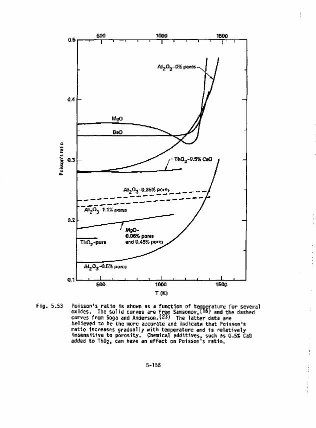
0.5 500 1000 1500

0.1

AI 2O 3-0% pores-

Al zO 3-0.5% pores

_. I . L . -L 500 1000 T O O

1500

Fig. 5.53 Poisson's ratio is shown as a function of temperature for several oxides. The solid curves are from Samsonov,(16) and the dashed curves from Soga and Anderson.! 2 3) The latter data are believed to be the more accurate and indicate that Poisson's ratio Increases gradually with temperature and is relatively Insensitive to porosity. Chemical additives, such as 0.5X CaO added to Th02i can have an effect on Poisson's ratio.

5-156

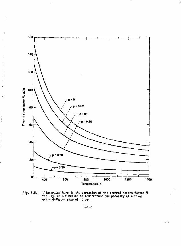
0 I 1 • I I I I I I I 1 400 600 800 1000 1200 1400

Temperature, K

Fig, 5.54 Illustrated here is the variation of the thermal stiess factor M for U 2 O as a function of temperature and porosity at a fixed grain diameter size of 10 un.

5-157

growth by the use of suitable chemical additives. This then points out an important area for future research on fabrication studies of Li,D to obtain materials with controlled grain sizes.

5-158

5.7 MATERIALS PROPERTIES AND INFORMATION TO SATISFY FIRST MALL ENVIRONMENTS

To permit a meaningful assessment of candidate first-wall structural materials to be conducted, an extensive data base covering the four classes of property information discussed below, i.e., physical properties, unirradiated mechanical properties, irradiation performance properties, and compatibility with expected special environments, such as breeding materials, and heat transport fluids, must be available for these materials. While the ideal situation is to select a material based on review of extensive data bases for numerous candidates, the usual situation is to select a material for which either (1) the available data base is complete enough to indicate that no obvious shortcomings (i.e., melting, vaporization, or total loss of ductility for prototypic irradiation conditions) exist; or (2) the available data base is lacking information in one (or more) important categories, but the remaining data base indicates strong advantages that outweigh the lack, of data.

The five classes of structural inaterials are: (1) light metals, i.e., Mg, Al, Ti, and their alloys, (2) ferritic (ferromagnetic) steels; (3) austenitic (paramagnetic) Fe-Cr-Ni and Fe-Mn-X (X may be one or more of the following: Cr, Ni, Mo, Cu, Nb, Al) steels; (4) austenitic (paramagnetic) nickel-based "superalloys", and (5) refractory metal alloys based on either V or Nb. After a cursory examination of the factors limiting the utility of the light-metal alloys, it was recognized that the relatively low-maximum use temperatures set forth below:

Mg alloys: t 340 K Al alloys: t 366 K Ti alloys: i. 727 !(

would seriously compromise the thermodynamic efficiency of any fusion-based power conversion system to an unacceptable degree. Hence, these alloys were eliminated from further consideration, and emphasis placed on development and evaluation of data bases for the remaining alloy classes.

5-159

Considering what physical properties are of prime importance, a signifi­cant fraction of stresses generated in both the first wall and blanket are thermally induced stresses, i.e., stress brought about by sudden temperature changes in the first wall due to plasma disruptions and the passage of slugs of either very cold or very hot working fluids in the blanket, causing local expansion or contraction of the structure with respect to its unperturbed attached adjoining members or regions. Hence, the perturbed portion of the structure is unable to undergo an unrestrained dimensional change, leading to the creation of "thermal-induced stress" in the restrained area or members.' ' In general, the resulting thermal stress, S t may be expressed by Eq. (5-46):

f [ f ^ " ] • S t (5-46)

where AT is the temperature difference over the member. The exact functional relationship depends on the nature of the constraint, geometric configur­ation of the restrained element, and the configuration of the temperature field with respect to the surfaces of the restrained element. Examination of Eq. (5.46) shows that the value of the elastic modulus, E, the instan­taneous coefficient of thermal expansion, a, and Poisson's ratio, v, are three physical properties that must be known for any candidate structural material. Since v ^ 0.25 to 0.3 for most materials {Ref. 25, for instance), and since calculation of thermal gradients across a structure requires a knowledge of the material's thermal conductivity, K, a physical property data base comprising E, a, K, and their variations with temperature was developed.

Figure 5.55 summarizes the variation with temperature of the elastic modulus, E, of class 2-5 candidate high temperature structural alloys, whose nominal compositions are given in Table 5.20. The data on the one ferritic steel, 2-1/4 Cr-1 Mo, the three austenitic Fe-Cr-Ni alloys (Types 304 and 316 stainless steels and the alloy 800H), and one of the nickel-based super-alloys (alloy 718) came from Ref. 26. The data on "Tenelon," a Fe-Mn-Cr austentic steel came frc-n Ref. 27. The data for V came from Ref. 28, while the data for various Nb alloys came from the following sources: Nb-l-Zr

5-160

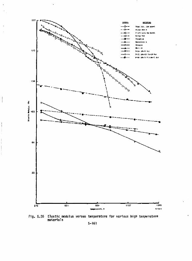
33 •

Type 304. 31* S W l A l l o y flCO ff

2 1/4 C(-l Ho Ste«l Alloy 719 Vinidlua H*itelloy X T»n«lon Hb-L 2r D-14 [Hb-5 Tr| D-31 (Wb-10 Tl-10 *to>

273 B2f 1365

F1g. 5.55 Elastic modulus versus temperature for various high temperature materials

5-161

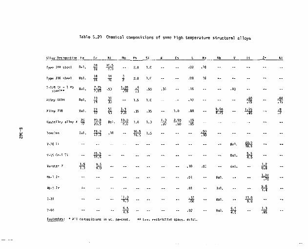
Table 5.20 Chemical compositions of some high temperature structural alloys

Alloy Designation re

Type 304 stee l Hal . j j j J 2 i l . . 2 . n 1.0 08 .10

Type 31fi steel Bal. jjl ^ | 2.0 1.0 — — .08 .10

-1/4 Cr - 1 Ho „ , 2.75 . . 1.20 .6 steel" B a ' - KDTJ " 5 0 - ^ 0 - 7 5

.50 .10 - .15

Alloy SOOH Bal. || |> ~ 1.5 1.0 - - .10 - - - ^ - -^|

Alloy 718 Bal. % |5 3 ^ .35 .35 - 1.0 .OB - £ f ° - ^ " f - $

"«*»•' >"<"*$ IfeS »"• ^ '•» '•» M ^ fM -- - -- -9.0 ,„ 16.5 , „ .50

T O - 1 0 " T O U 0 3 0 lenelon Bal. | f ^ .10 -- - ^ 1.0

V-20 ri

V-15 Cr-5 Ti

M hi Vanstar 7 T B JT3 - , 0 - 0 1

Hl>-1 Zr — 01 — Bal.

lib-5 Zr -- — — .01 — Bal.

" J ^CTJ 708 •• B a l-

B-66 j i | .02 — Bal.

Footnotes: * fill compositions in wt. percent. ** Less restrictive specs, exist.

Ba). 20.5 TO -Ba l . 5.5

1 3 " Bal . -- TH

- " ^ -- " ft -- 11.0

9.0 " 5.5 4.5 - ^

(Refs. 29-31), Nb-5-Zr (Ref. 32), Nb-10 Ti-10 Mo (Refs. 32-33), and Nb-5V-5 Mo-1 Zr (Ref. 34). Note that the iron- and nickel-based alloys have higher elastic modulus values (•»• 127.6 GPa) at 1366 K than the refractory metal alloys (-«- 60.7-110.3 GPa}.

Figure 5.56 summarizes the variation with temperature of the instanta­neous coefficient of thermal expansion, a, of class 2-5 candidate high temperature structural alloys. The data on the 2-1/4 Cr-1 Mo ferritic steel, the three austjnitic Fe-Cr-Ni alloys (Types 304 and 316 stainless steels and alloy 800H) and one of the nickel-based alloys {alloy 718) came from Ref. 26. The data for nickel-based Hastelloy X came from Ref. 35. The data on the Fe-Mn-Cr austeiitic alloy (Tenelon) came from Ref. 28. The data on the various Nb-based alloys came from the following references: Nb-1 Zr (Refs. 29, 36), Nb-10 Ti-10 ^ (Ref. 37), and Nb-5 V-5 Mo-1 Zr (Ref. 34). Note that the ferritic and austenitic alloys have a values at 811 K of about 14.8 to 21.3 x ID" 6 K, while the Nb alloys have a values of about 7.6 x 10 K at the same temperature.

Figure 5.57 summarizes the temperature variation of thermal conductivity of various class 2-5 candidate high temperature structural alloys. The data on the 2-1/4 Cr-1 Mo ferritic steel, the three austenitic Fe-Cr-Ni alloys (Types 304 and 316 stainless steel and alloy 800H) and one of the nickel-based alloys (alloy 718) came from Ref. 25. The data on the one Nb alloy (Nb-1 Zr) came from Ref. 38. Note that the a:T behavior for the austen­itic (face-centered cubic) alloys are all similar, starting at about .086-.138 watts/cm K at room temperature and increasing monotonically to a value range of .241-.267 watts/cm K at about 1089 K, The a:T behavior for the two body centered cubic alloys, Nb-1 Zr Nb alloy and 2-1/4 Cr-1 Mo ferritic steel are much different from that exhibited by the austenitic alloys, starting at room temperature at values of about .448 and .362 watts/cm K, respectively, and increasing with increasing temperature in the former case versus decreasing with increasing temperature in the latter case.

Given the values of E and a at 1089 K, and assuming a value of v of 0.3,

5-163

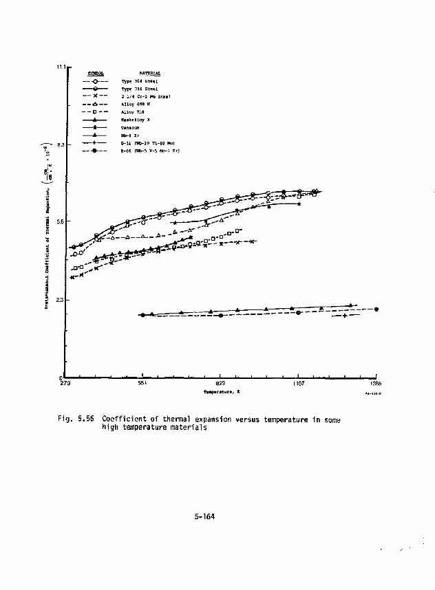
SYMBOL MATERIAL

—-o-— Type 304 St«*tl

Type 316 S t « l

Type 304 St«*tl

Type 316 S t « l

— X — 2 1/4 Ci-1 Ha S t e e l

— A — Alloy 500 H

- - a - - Alloy 718

Hast* Hoy X

Tfrtelon

Hft-1 It

E>-31 (Hb-10 Tl-10 Mo)

— * — Hast* Hoy X

Tfrtelon

Hft-1 It

E>-31 (Hb-10 Tl-10 Mo)

Hast* Hoy X

Tfrtelon

Hft-1 It

E>-31 (Hb-10 Tl-10 Mo)

— .#.— B-66 (Nb-5 V--5 Ho-1 Zr]

~&^&^P*fr

S 23

273 551 829 TmpciAture, X

1107 1385

Fig. 5.56 Coefficient of thermal expansion versus temperature in some high temperature materials

5-164

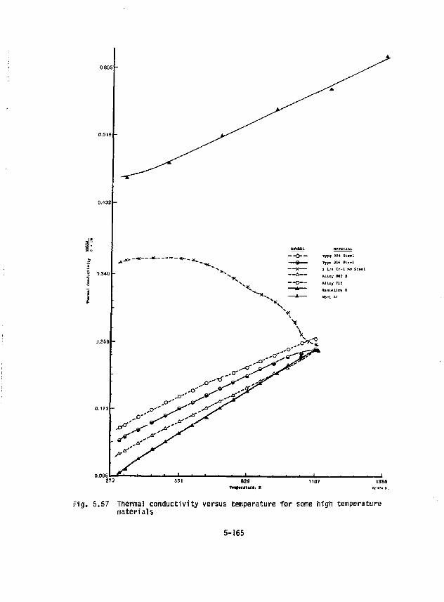
SYMBOL MATERIAL

--o— Typ»* )04 S t e e l

^-Q Type 31* S t e e l

X 2 1/4 Cr-1 K> S t e e l A A l l a y 840 H

G — A l l a y 719

* H a n t e l l e y X

A H6-1 IE

Fig. 5.57 Thermal conductivity versus temperature for some high temperature materials

5-165

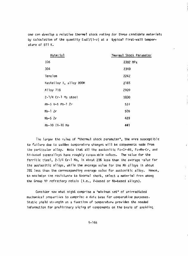
one can develop a relative thermal shock rating for these candidate materials by calculation of the quantity EaAT/(l-v) at a typical first-wall temper­ature of 811 K.

Material 316 304 Tenelon Hastelloy X, alloy S00H Alloy 718 2-1/4 Cr-1 Mo steel JVb-5 V-5 Mo-1 Zr

Nb-1 Zr Nb-5 Zr Nb-10 Ti-10 Mo

Thermal Shock Parameter 2382 MPa 2340 2242 2165 2109 1830 531 506 489 441

The larger the value of "thermal shock parameter", the mnre susceptible to failure due to sudden temperature changes will be components made from the particular alloy. Note that all the austenitic Fe-Cr-Ni, Fe-Mn-Cr, and Ni-based superalloys have roughly compaFable values. The value for the ferritic tteel, 2-1/4 Cr-1 Mo, is about 23% less than the average "alue for the austenitic alloys, while the average value for the Nb alloys is about 78% less than the correseponding average value for austenitic alloy. Hence, to maximize the resistance to thermal shock, select a material from among the Group VA refractory metals (i.e., V-based or Nb-based alloys).

Consider now what might comprise a "minimum set" of unirradiated mechanical properties to comprise a data base for comparative purposes. Static yield strength as a function of temperature provides the needed information for preliminary sizing of components on the basis of avoiding

5-166

permanent deformation {yielding) during short-time operation. Since the design life has been set at 3 years (or 26299 hours) of full-power operation, the stress to rupture and stress to produce 1£ total deformation in a time of 3 years as functions of temperature enable the effects of time-dependent deformation to be evaluated. Lastly, since the plant will be subject to some small number of perturbations from steady-state operation dur>ng the 3-year life of the blanket, a knowledge of the low-cycle strain-controlled fatigue performance of candidate structural material is desirable.

Information on the minimum expected yield strength (S):temperature (T) behavior of several candidate structural materials from classes 2-5 is presented in Fig. 5.58. The method of obtaining "minimum expected S :T" trends is the same as that used in derivation of ASME Boiler and Pressure Vessel Code design allowables (Ref. 39). Data for the three Fe-Cr-Ni austenitic alloys (Types 304 and 316 stainless steels and ailoy 80DH) was taken from Ref. 26, while data on the Fe-O-Mn austenitic alloy (Tenelon) was taken from Ref. 27. Data for the two nickel-based superalloys came from Ref. 27 (alloy 718) and Ref. 35 (Hastelloy X). Data on the V-20 T alloy came from Refs. 40-44, while data for the Vanstar-7 alloy came from Refs. 41-42 and 45-48. Data on the Nb-1 Zr alloy cane from Refs. 40-41 and 49-54, while data on the Nb-10 Ti-10 Mo alloy came from Refs. 32-33, 37, and 54-55. Data on the Nb-5 Mo-5 V-l Zr alloy came from Refs. 34 and 56-61.

Examination of the S :T information presented on Fig. 5.58 indicates that, referred to Type 304 austenitic stainless steel at 811 K, the S values of the other high temperature stnxtural materials rank as follows:

5-167

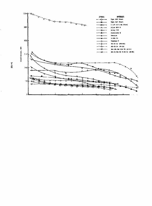
SJfMBOI MAXEftlAL

0 Type 304 S t e e l

Type 316 S t e e l

2 1/4 Cr-1 Mo S t e e l

Al loy BOO H

Type 316 S t e e l

2 1/4 Cr-1 Mo S t e e l

Al loy BOO H A

Type 316 S t e e l

2 1/4 Cr-1 Mo S t e e l

Al loy BOO H

— -a Alloy 718

Haste l loy X Haste l loy X

* Tentlon

V-2Q» Tt V-2Q» Tt

-o Vanstai-7

— 0 - — Nb-U Zr (FS-80) Hb-5% Zr ID-14} Nb-U Zr (FS-80) Hb-5% Zr ID-14}

Nb-lOt Ho-lOi Ti [D-31) Nb-lOt Ho-lOi Ti [D-31)

Hb-5% lto-5% V - l t Zr (B-66J

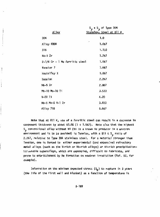
S * S of Type 304 Alloy Stainless Steel at 811 K

304 1.0 Alloy 800H 1.067 316 1.133 Nb-1 Zr 1.267 2-1/4 Cr - 1 Mo ferritic steel 1.567 Vanstar 7 1.667 Hastelloy X 1.867 Tenelon 2.267 Nb-5 2r 2.867 fib-10 Mo-10 T i 3.533 V-20 Ti 4.20 Nb-5 Mo-5 V-l Zr 3.933 Alloy 718 8.667

Note that at 811 K, use of a ferritic steel can result in a decrease in component thickness by about 63.8% (1 f 1.567). Note also that the highest S conventional alloy without Ni (Ni is a known He producer in a neutron environment and is to ba avoided) is Tenelon, with a 811 K S ratio of 2.267, relative to Type 304 stainless steel. For a material stronger than Tenelon, one is forced to either experimental (and expensive) refractory metal alloys (such as the V-rich or Nb-rich alloys) or Ni-rich precipitation-h2;-Jenable superalloys, which are expensive, difficult to fabricate, and prone to embrittlement by He formation on neutron irradiation (Ref. 62, for example).

Information on the minimum expected stress (S R) to rupture in 3 years (the life of the first wall and blanket) as a function of temperature is

5-169

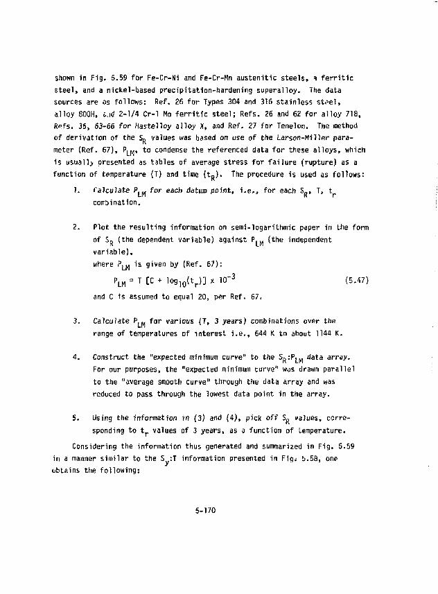
Shown in Fig. 5.59 for Fe-Cr-Ni and Fe-Cr-Mn austenitic steels, =» ferritic steel, and a nickel-based precipitation-hardening superalloy. The data sources are as follows: Ref, 26 for Types 304 and 316 stainless stviel, alloy 800H, i.xl 2-1/4 Cr-1 Mo ferritic steel; Refs, 26 and 62 for alloy 718, ftpfs. 35, 63-66 for Hastelloy alloy X, and Ref. 27 for Tenelon. The method of derivation of the 5 R values was based on use of the Larson-Miller para­meter (Ref. 67), P|f.« to condense the referenced data for these alloys, which is usually presented as tables of average stress for failure (rupture) as a function of temperature (T) and time (t R). The procedure is used as follows:

J. Calculate P.„ for each datum point, i.e., for each S , T, t combination.

2. Plot the resulting information on semi-logarithmic paper in the form of S R (the dependent variable) against P | M (the independent variable), where P, M is given by (Ref. 67):

P L H = T [C + log 1 Q(t r)] x 10" 3 (5.47) and C is assumed to equal 20, per Ref. 67.

3. Calculate P,M far various (T, 3 years) combinations over the range of temperatures of interest i.e., 644 K to about 1144 K.

4. Construct the "expected minimum curve" to the S R:Pi M data array. For our purposes, the "expected minimum curve" was drawn parallel to the "average smooth curve" through the data array and was reduced to pass through the lowest data point in the array.

5. Using the information in (3) ant) (4), pick off S R values, corre­sponding to t r values of 3 years, as a function of temperature.

Considering the information thus generated and summarized in Fig. 5.59 in a manner similar to the S :T information presented in Fig.- b.58, one obtains the following:

5-170

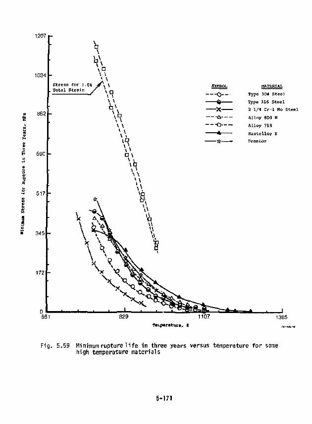
1207 F 1034

Stress For L Total Straii

862

690 h

I 5171-

3451-

172 h

1-0* / \ \ SYMBOL MATERIAL

—-o— Type SO* Steel Type 316 Steel w Type SO* Steel Type 316 Steel

X 2 1/4 Cr-1 Mo Steel — • & - - Alloy 800 H — -O — Alloy 71B

Hastelloy X Tenelon i-

Alloy 71B Hastelloy X Tenelon

1385 T«#cratur* r K

Fig. 5.59 Minimum rupture l i f e in three years versus temperature for some high temperature materials

5-171

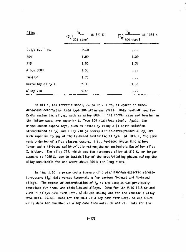
1IM S» ,t e l l K K 304 steel

2-1/4 Cr- 1 Mo 0.60 304 1.00 316 1.50 Alloy 800H 1.65 Tenelon 1.75 Hastelloy alloy X 2.00 Alloy 718 5.45

1.00 1.33

3.33

At 811 K, the ferritic steel, 2-1/4 Cr - 1 Mo, is weaker in time-dependent deformation than Type 304 stainless steel. Both Fe-Cr-Ni and Fe-O-Mn austenitic alloys, such as alloy 800H in the former case and Tenelon in the latter case, are superior to Type 304 stainless steel. Again, the nickel-based superalloys, such as Hastelloy alloy X (a solid solution strengthened alloy) and alloy 718 (a precipitation-strengthened alloy) are much superior to any of the Fe-based austenitic alloys. At 1089 K, the same rank ordering of alloy classes occurs, i.e., Fe-based austenitic alloys lower and a Ni-based solid-solution-strengthened austenitic Hastelloy alloy X, higher. The alloy 718, which was the strongest alloy at 811 K, no longer appears at 1089 K, due to instability of the precipitating phases making the alloy unsuitable for use above about 894 K for long times.

In Fig. 5.60 is presented a summary of 3 year minimum expected stress-to-rupture (S R) data versus temperature for various v-based and Nb-based alloys. The method of determination of S R is the same as was previously described for iron- and nickel-based alloys. Data for the U-15 Ti-5 Cr and V-20 Ti alloys came from Refs. 41-43 and 45-46; and for the Vanstar 7 alley from Refs. 45-46. Data for the Nb-1 Zr alloy came from Refs. 54 and 68-74 while data for the Nb-5 Zr alloy came from Refs. 32 and 71. Data for the

5-172

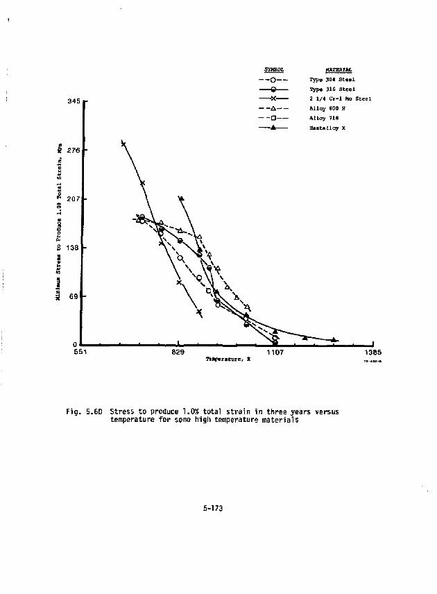
345 r

Si 276 f-

207

1381-

SYHBOL

- - o — — ©

X - - A — — a —

A

HMERIhL

Type 304 S t e e l

Type 316 S t e e l

2 1/4 Cr-1 Mo S t e e l

A l loy 800 H

W l o y 718

a a s t e U o y X

1385

F ig . 5.60 Stress to produce 1.0% tota l s t ra in in three years versus temperature fo r some high temperature mater ia ls

5-173

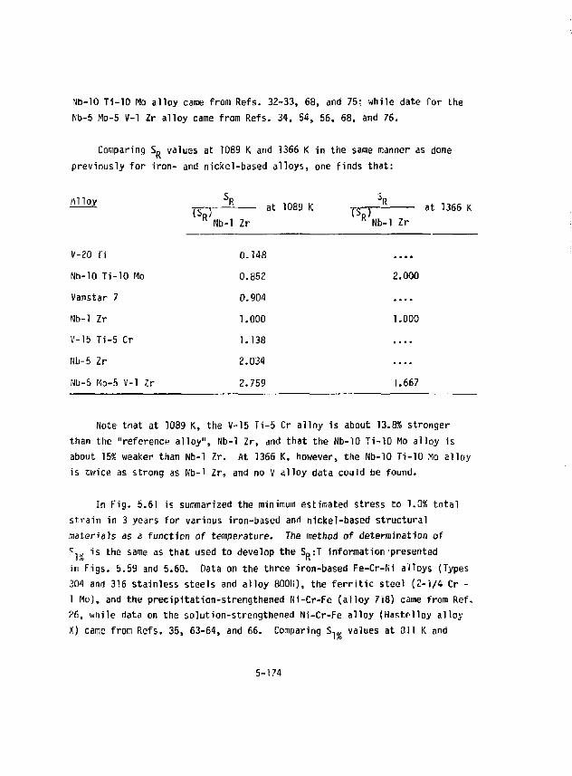
Nb-10 Ti-10 Mo alloy came from Refs. 32-33, 68, and 75: while date for the Nb-5 Mo-5 V-l IT alloy came from Refs. 34, 54, 56, 68, and 76.

Comparing S R values at 1089 K and 1366 K in the same manner as done previously for iron- and nickel-based alloys, one finds that;

Alloy \ . i n f l q ^ , ^R Tsp a t 1 0 8 9 K vqr~

at 1089 K ; $ \ •• at 1366 K Nb-1 Zr R Nb-1 IT

V-20 Ti 0.148 Nb-10 Ti-10 Mo 0.852 2.000 Vanstar 7 0.904 Nb-1 Zr 1.000 1.Q0O V-15 Ti-5 Cr 1.138 Nb-5 Zr 2.034 Nb-5 Mo-5 V-l Zr 2.759 1.667

Note that at 1089 K, the V-15 Ti-5 Cr alloy is about 13.8% stronger than the "reference alloy", Nb-1 Zr, and that the Nb-'lO Ti-10 Mo alloy is about 15% weaker than Nb-1 Zr. At 1366 K, however, the Nb-10 Ti-10 Mo alloy is twice as strong as Nb-1 Zr, and no V alloy data could be found.

In Fig. 5.61 is summarized the minimum estimated stress to 1.0% total strain in 3 years for various iron-based and nickel-based structural materials as a function of temperature. The method of determination of S.„ is the same as that used to develop the 5 D:T information presented in Figs. 5.59 and 5.60. Data on the three iron-based Fe-Cr-Ni alloys (Types 304 and 316 stainless steels and alloy 800H), the ferritic steel (2-1/4 Cr -1 Mo), and the precipitation-strengthened Ni-Cr-Fe (alloy 7i8) came from Ref, 26, while data on the solution-strengthened Ni-Cr-Fe alloy (Hastf-lloy alloy X) came from Refs, 35, 63-64, and 66. Comparing S, £ values at 311 K and

5-174

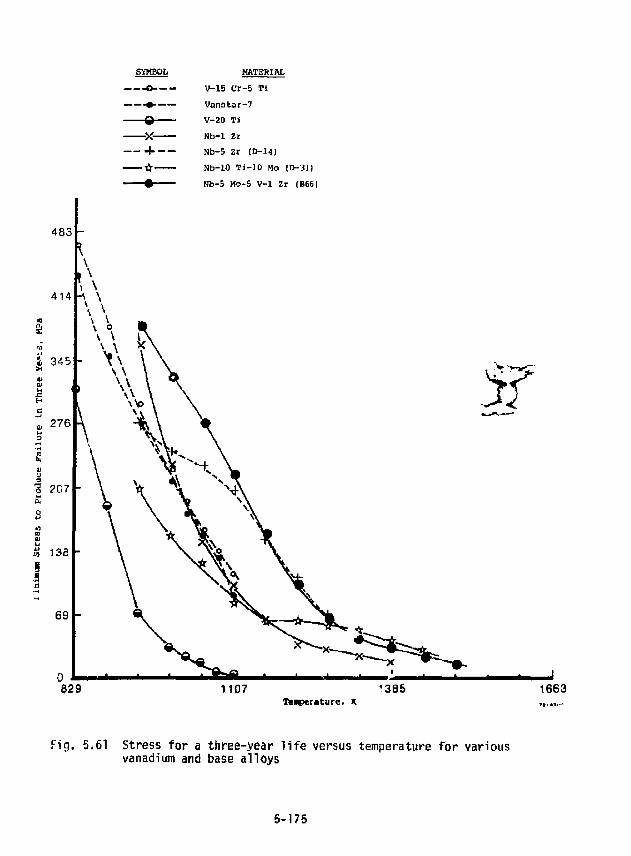
SYMBOL MATERIAL 0 V-15 Cr-5 Ti • Vanstar-7

v-20 Ti Nb-1 Zr v-20 Ti Nb-1 Zr

(. Nb-5 Zr (D-14)

• Nb-10 Ti-10 Ho (D-3]) Nb-5 Ho-5 V-l Zr (B66I

4B3 -

414

345

276

•g 207

133 -

629 1107

if

s=%. !385 1663

Temperature, K

Fig. 5-61 Stress for a three-year life versus temperature for various vanadium and base alloys

5-175

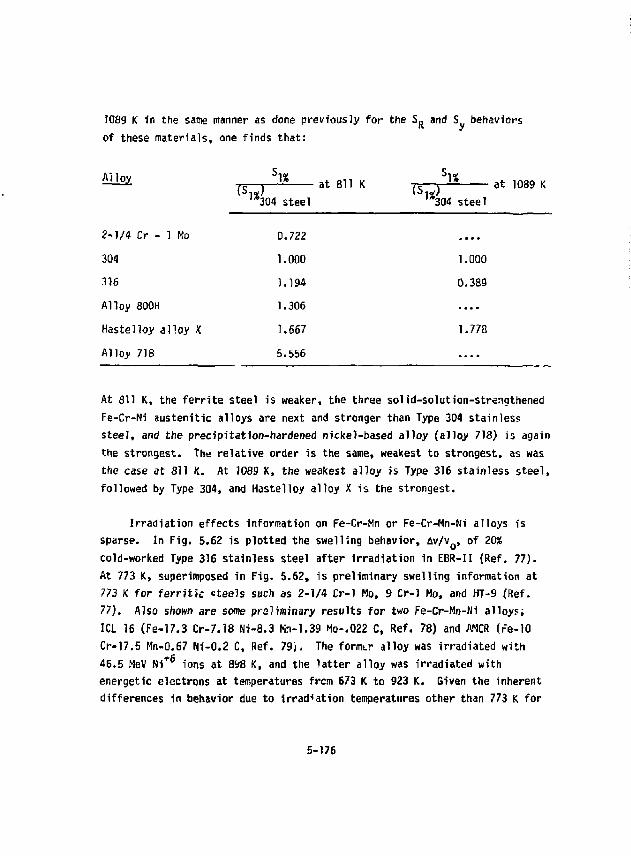
1089 K in the same manner as done previously for the S„ and S behaviors of these materials, one finds that:

Alloy h% „<.<,,,„ S 1 * TsTT) a t 8 l l K Ts3T^ a t l 0 8 9 K

'*304 steel '*304 steel

2-1/4 Cr - 1 Mo 0.722 304 1.000 1.000 316 1.194 0.389 Alloy 800H 1.306 Hastelloy alloy X 1,667 1.778 Alloy 718 5.556 ....

At 811 K, the ferrite steel is weaker, the three solid-solution-strenqthened Fe-Cr-Ni austenitic alloys are next and stronger than Type 304 stainless steel, and the precipitation-hardened nickel-based alloy (alloy 718) is again the strongest. Th« relative order is the same, weakest to strongest, as was the case at 811 K. At 1089 K, the weakest alloy is Type 316 stainless steel, followed by Type 304, and Hastelloy alloy X is the strongest.

Irradiation effects information on Fe-Cr-Mn or Fe-Cr-Mn-Ni alloys is sparse. In Fig. 5.62 is plotted the swelling behavior, Av/v , of 20% cold-worked Type 316 stainless steel after irradiation in EBR-II (Ref. 77). At 773 K, superimposed in Fig. 5.62, is preliminary swelling information at 773 K for ferritk steels such as 2-1/4 Cr-1 Mo, 9 Cr-1 Ho, and HT-9 (Ref. 77). Also shown are some preliminary results for two Fe-Cr-Mn-Ni alloys; ICL 16 (Fe-17.3 Cr-7.18 Ni-8.3 Nn-1.39 Mo-.022 C, Ref. 78) and AMCR (re-10 Cr-17.5 Mn-0.67 Ni-0.2 C, Ref. 79j. The formtr alloy was irradiated with 46.5 MeV Ni ions at 8SJ8 K, and the latter alloy was irradiated with energetic electrons at temperatures frcm 673 K to 923 K. Given the inherent differences 1n behavior due to irradiation temperatures other than 773 K for

5-176

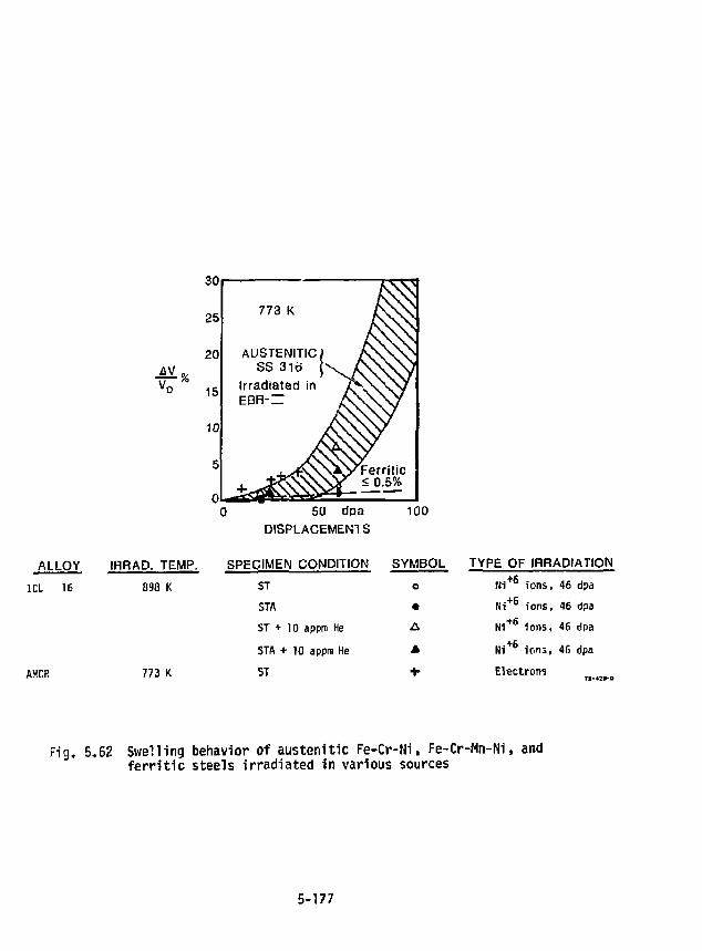
AV

30

25

20

• %

o 15

10

773 K H AUSTENITIC/

SS 316 ( \ Irradiated in EBR-Z: i

+ ^ j ^ ^ \ X ^ ^ VFerritic y < 0.5%

50 dpa 100 DISPLACEMENTS

ALLOY

ICL 16

AHCR

IRRAD. TEMP. SPECIMEN CONDITION SYMBOL

898 K ST o STA • ST + 10 appm He A STA + 10 appm He A

773 K ST +

TYPE OF IRRADIATION

N1 ions, 46 dpa

Ni ions, 46 clpa

NI ions, 46 dpa

Ni ion i , 46 dpa

Electrons

Fig. 5.62 Swelling behavior of austenitic Fe-Cr-Ni, Fe-Cr-Mn-Ni, and f e r r i t i c steels irradiated in various sources

5-177

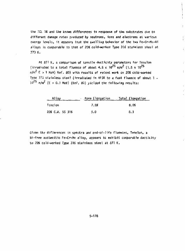
the JCL 16 and the known differences in response of the substrates due to different damage rates produced by neutrons, ions and electrons at varicus evergy levels, it appears that the swelling behavior of the two Fe-Cr-Mn-Ni alloys is comparable to that of 20% cold-worked Type 316 stainless steel at 773 K.

At 811 K, a comparison of tensile ducticity parameters for Tenelon (irradiated to a total fluence of about 4.5 x 1 0 2 5 n/m2 (1.5 x 1 0 2 5

n/m2 E > 1 MeV) Ref. 80) with results of recent work on 20% cold-worked Type 315 stainless steel (irradiated in HFIR to a fast fluence of about 1 .; 1 0 ? & n/m2 (E > 0.T MeV) (Ref. 81) yielded the following results:

Alloy form Elongation Total Elongation Tenelon 7-5% 8.0% 20% C.W. SS 316 5.0 8.3

Given the differences in spectra and end-of-1'ife fluences, Tenelon, a Ni-free austenitic Fe-Cr-Mn alloy, appears tc exhibit comparable ducticity to 20% cold-worked Type 316 stainless steel at 811 K.

5-178

5.8 THE INFLUENCE OF WASTE DISPOSAL ON MATERIAL SELECTION

One of the important considerations in the design of fusion reactors is the impact of materials selection upon the generation and disposal of radio­active wastes from neutron activation of structural materials. Recent developments in regulations for the disposal of radioactive wastes (NRC-proposed regulation 10CFR61, "Licensing Requirements for Land Disposal of Radioactive Hastes") furnish a basis for classifying wastes with respect to composition, form, and method of disposal. The key factor from 10CFP.61 for reactor designers is the limit on specific activity for a given disposal method and for each combination of radioactive isotopes in waste. This limit can be combined with predicted activities for elemental components in structural alloys to give an index of waste disposal ratings (WDR). This is:

MDR = 2 fijl A(i) and L(i) in units of curies/m3

where A(i) is the activity of the i isotope in an alloy and L(i) is the limit from 70CFR6T for the i t h ;-otope. If WDR <_ 1, then according to 10CFR61, the waste could be disposed of by near-surface burial as low-level waste. If MDR >_ 1, the disposal could not be near-surface but would have to be by some accepted method for "high" level waste such as deep geologic disposal.

The WDR for several steels that might be used in fusion reactors have (82 fl3l been calculated.1 * ' The list of these steels and their nominal elemental

compositions are given in Table 5.21. The predicted specific activities for the critical elements for long-term disposal are snuwn in Table 5.22 for the first wall of one of the conceptual reactor designs done on MARS. The corre­sponding WDR's for this design are shown in Table 5.23. Froir the column for Total Alloy in Table 5.23, it can be seen that first-wall alloys 5, 7, 10 and 11 are the only ones tnat could be directly disponed of by near-surface burial. All the others would have to be processed to make WOR £ 1. The processing might be simple dilution in a concrete matrix. The amount of dilution would be in direct properties to the original WOR. Thus the alloy

5-179

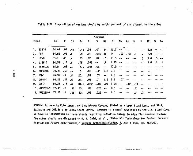
Table 5.21 Composition of various steels by weight percent of the element in the alloy

Element Steel Fe C Si Hn P S Ni Cr Nb Al N V MO W Cu

1. SS316 64.44 .06 .46 1.43 .03 .01 14 16.7 2. PCA 64.68 .05 .5 1.8 .01 .005 16 14 .03 .03 .01 — 2.0 — — 3. HT-9 85.1 .2 .4 .55 .02 .02 .5 11.5 — — — .3 1.0 .5 — 4. 2.25-1 94.58 .15 .5 .45 .035 — .5 2.25 ~ — — — 1.0 .1 .5 5. TENELON 68.0 .08 .3 U.5 .045 .03 — 17.0 — — — — — — — 6. NOMAGNE 79.35 .65 .5 15. .03 .02 2.2 2.2 — — — — ~ ~ — 7. NM-1 76.92 .5 .5 20. .05 .03 ~ 2.0 ~ -- — — — — — 8. 25-5-1 66.22 .17 .6 26. .03 .01 1.2 5.5 .07 — — — ~ — ~ 9. 32-7 60.24 .14 .6 31.6 .022 .006 .23 7.04 - .12 .13 — — — -10. JUS289-N 72.45 .6 .65 20. .08 .025 — 6.0 — — .2 — — — -11. JUS289-V 72.15 .6 .65 20. .08 .025 ~ 6.0 ~ -. .2 .3 — — —

NOMAGNt is made by Kobe steel, NM-1 by Nippon Korean, 25-5-1 by Nippon Steel Ltd., and 32-7, JUS289-N and 0US289-V by Japan Steel Works. Tenelon is a steel developed by the U.S. Steel Corp. We have no information on these steels regarding radiation damage In high flux neutron fields. The other steels are discussed in R. E. Gold, et al., "Materials Technology for Fusion: Current Startup and Future Requirfimaote." HiiclBar TgchnDlPQy./Fusinn, 1, April )58J, pp. 1B5-2i7.

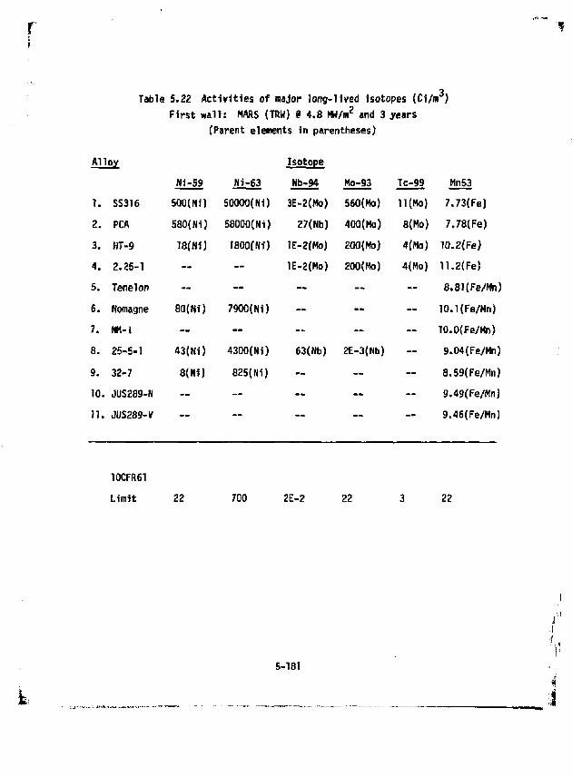
Table 5.22 Activities of major long-lived isotopes (Ci/m ) First wall: MARS (TRW) » 4.8 MW/mZ and 3 years

(Parent elements in parentheses)

Alloy Isotope Ni-59 Hi-63 Nb-94 Mo-93 Tc-99 Mn53

1. SS316 500(Ni) 50000(N1) 3E-2(Mo) 560(Ho) 11(Ho) 7.73(Fe) 2. PCA 580{Ni) 58000(Ni) 27(Nb) 400(Mo) 8(Ho) 7.78(Fe) 3. MT-9 IfifNiJ 1800(Ni) lE-2(Mo) 200(Mo) 4(Mo) 10.2(Fe) 4. 2.25-1 — — lE-2(Mo) 200(Mo) 4(Ho) 11.2(Fe) 5. Tenelon — — — ~ — 8.81(Fe/Hn) 6. Nomagne 80(Ni) 79O0(N1) ~ — — 10.1{Fe/Mn) 7. NK-i — ~ — ~ ~ 10.0(Fe/Mn) 8. 25-5-1 43(Ni) 4300(Ni) 63(Nb) 2E-3(Nb) — 9.04(Fe/Mn) 9. 32-7 8(Ni) 825(Ni) ~ ~ — 8.59(Fe/Mn) 10. JUS289-N — — — ~ ~ 9.49(Fe/Mn) 11. JUSZ89-V ~ — — — — 9.46(Fe/Hn)

10CFR61 Limit 22 700 2E-2 22 3 22

5-181

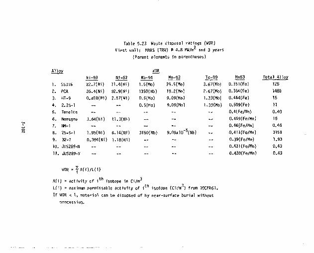
Table 5.23 Waste disposal ratings (WPR) First wall: MARS (TRW) 0 4.8 MW/m2 and 3 years

(Parent elements 1n parentheses)

Alloy WDR Ni-59 Ni-63 Nb-94 Ho-93 Tc-99 Mn53 Total Alloy

1. SS316 22.7(Ni) 71.4(Ni) 1.5(Mo) 25.5(Mo) 3.67(Mo) 0.351(Fe) 125 2. PCA 26.4(Ni) 82.9(Ni) 1350(Nb) 18.2(Mo) 2.67(Mo) 0.354(Fe) 1480 3. HT-9 0.818(tti) 2.57(Ni) 0.5(Mo) 9.09(Mo) 1.33(Mo] 0.464(Fe) 15 4. 2.25-1 ~ — 0.5(Mo) 9.09(Mo) 1.33(Mo) 0.509(Fe> 11 5. Tenelon — — — — — 0.4(Fe/Mn) 0.40 6. Namagne 3.64(Ni) U.3(Mi) — — — 0.459(Fe/Mn) 15 7. NM-1 — — — - -- 0.46(Fe/Mn) 0.46 8. 25-5-1 1.95(Ni) 6.14(Ni) 3150(Nb) 9.09xlO"5(Nb) .. 0.411(Fe/Hn) 3159 9. 32-7 0.364(Ni) 1.18(Ni) -- — — 0.39(Fe/Mn) 1.93 10. JUS289-N — — — — — 0.431(Fe/Mn) 0.43 71. JU5289-V

WDR = ? A( i)/L(i)

0.430(Fe/Mn) 0.43

A(i) = activity of i isotope in Ci/m L(i) = maximum permlssable activity of 1 isotope (Ci/m ) from 10CFR61. If WDR < 1, material can be disposed of by near-surface burial without

processing.

25-5-1 would require by far the most dilution because of its niobium content. The alloy PCA requires the next largest dilution, again primarily because of niobium. Stainless steel 316 requires the third largest dilution because of its high nickel and molybdenum content. The tables indicate that nickel and molybdenum are undesirable for long-term waste disposal in all the alloys. The high manganese alloys without nickel and/or molybdenum would be highly desirable from a waste management viewpoint since they would require no waste processing except for transportation packaging.

5-183

5.9 SUMMARY

The solid Li^O Canister blanket concept appears t o offer many advantages over previous designs. The main advantages are summarized below:

(a) The relatively cool structural envelope of each Canister can use a steel alloy such as Tenelon which has much lower radioactivation than ferritic or stainless steels.

(b) The Canister acts as the primary blanket pressure vessel with good structural safety factors.

(c) The solid Li,0 tritium breeder material is separated from the main helium coolant flow by putting it in tubes inside the Canister. This greatly facilitates tritium separation and isolation of the tritium from the thermochemical plant.

(d) These tubes can run at very high temperatures and still be made of Tenelon, because they are almost pressure-balanced and hence experience very low stresses.

(e) The design of the blanket as a bank of staggered tubes allows us to take advantage of the very good heat transfer and low pumping power requirements of a cross-f7ow-type heat exchanger.

(f) The tube bank can be designed as a multi-pass heat exchanger so that the main helium inlets and exits can be conveniently located at the back of the blanket Canisters.

(g) The hot shield is designed as a set of staggered rods which are a direct extension of the tube bank. This provides a low pressure drop flow path for the helium while at the same time eliminating most neutron streaming.

5-184

(h) The blanket can be proof-tested initially at the Canister level; this is a very convenient small-size unit. The next level of test can be at the ring module level which consists of a compact assembly of 18 Canisters.

(i) Two ring modules fit in the region between each two centra? eel? magnet coils in such a way that assembly and disassembly is possible with simple motions without moving the magnets.

(j) The Canisters of each ring module are mutually supporting along the sides of the Canisters, resulting in reduced structural requirements. The use of common headers minimizes the possibility of total depressurization of one Canister and a domino-type failure of the remaining Canisters.

Many detailed design questions remain to be answered. However, this blanket concept has survived a critical review and remains one of the most attractive concepts we have seen in the past 15 years.

5-185

Section 5 Nomenclature

speed of sound in helium area flow channel total cross-sectional area specific heat of helium diameter of the He purge hole in the Li,0 inner diameter of the tube diameter of the LigO cartridge outer diameter of the tube diameter hydraulic diameter fraction of Li^O in the tube bank fraction of structure in the tube bank fraction of 100* theoretical density of the Li'20 total "void" fraction in the tube bank Darcy-Weisbach friction factor Fanning friction factor = f/4 mass flux, pv average convective heat transfer coefficient thermal conductivity of helium thermal conductivity of insulation thermal conductivity of LioO thermal conductivity of the large pipe walls thermal conductivity of the tube wall mass flow rate

5-186

Nu = Nusselt number P = pressure Pr = Prandtl number

Q = heat flow or input

q = heat flux r = radius measured from the first wall at the Canister

separation point * = decay length for internal heat generation in Li z0 *

rs = decay length for internal heat generation in the tube material

Re = Reynolds number, GD^/u s = path length along the flow in the canister st = transverse stagger of the tube bank s1 = longitudinal stagger of the tube bank t = thickness of the first wall

l9 = annular gap for helium purge flow

*L = thickness of the LioO annular cartridge

\ = width of the minimum spacing between tubes

*w = thickness of the tube wall T = temperature TB = bulk mean temperature of the helium Tw = wall temperature V = velocity V = volume w = internal heat generation

0,L = internal heat generation in the Li 20 at r = 0 = internal heat generation in the structure at r = 0

5-187

y s ratio of specific heats, C /C y

r N = neutron wall loading 6 = height of the first wall coolant passage e t = fraction of the tube bank unit cell occupied by the tube u = helium dynamic viscosity p = helium density

5-188

References for Section 5

1. T. Elleman, University of North Carolina, personal communication via E. Dalder, Lawrence Livermore National Laboratory (February 1982).

2. K. Okula and D. K. Sze, "Tritium Recovery from Solid Breeders," University of Wisconsin (Madison), Rept. UWFDM-351 (April 1980).

3. R. Hickman, "Some Problems with Tritium in Fusion Reactors," Technology of Controlled Thermonuclear Fusion Experiments. U.S. AEC Reot. CONf-721111 (ApHT 1374).

4. Chemical Engineers' Handbook, R. Perry and C. Chilton, Eds., (McGraw-Hill, New York, 1973) 5th ed., pp. 3-230.

5. R. Reid, J. Praushitz and F. Sherwood, The Propurties of Gases and Liquids (McGraw-Hill, New York, 1971).

6. J. Hirschfelder, C. Curtis and R. Bird, Molecular Theory of Bases and Liquids (J. Wiley, New York, 1954).

7. Chemical Engineering Division Annual Technical Report, Argonne National Laboratory, ANL-82-23, p. 135 (1981).

8. T. R. Hill, "ONETRAN, A Discrete Ordinates Finite Element Code for the Solution of the One-Dimensional Multigroup Transport Equation," LA-5900-MS, Los Alamos National Laboratory (June 1975). (The pre­release availability of 0NE0ANT to the study is a result of the courtesy of Donald J. Dudziak of Group T-l, Los Alamos National Laboratory.)

9. R. E. Alcouffe, "Diffusion Synthetic Acceleration Methods for the Diamond-Difference Discrete Ordinates Equation," Nucl. Sci. Eng. 64, 344 (1977). —

10. R. E. MacFa-lane and R. J. Bennett, I.ANL Internal Memo T-2-L, Los Alamos National Laboratory (August 24, 1978).

11. C. Baker, et al., "STARFIRE - A Commercial Tokamak Fusion Power Plant Study," ANL-FPP-80-1, Argonne National Laboratory (1980).

12. T. Takahashi and T. Kikuchi, "Porosity Dependence on Thermal Diffusivity and Thermal Conductivity of Lithium Oxide Li?0 from 200 to 900°C," J. Nucl. Mater., 9]_, 93(1980). ~~

13. T. Kurasawa, "Thermal Expansion of Lithium Oxide," private communication from T. Kurasawa, Japan Atomic Energy Research Institute, Tokai-mura, Japan, November 24, 1981, submitted for publication to J. Nucl. Mater.

5-189

14. 0. H. Krik&rian, "Esti/ttatier? &f Heat Capacities and other Thermodynamic Properties of Refractory Borides," Lawrence Liverrcore National Laboratory, Lievermore, CA, UCRL-51043, (April 27, 1971).

15. S. Nasu, K. Fukai, and T. Tanifuji, "Microhardness and Microst.ructures of Neutron Irradiated Li^O Pellets," J. Nucl. Hater.t 28, 254(1978).

16. "The Oxide Handbook," edited by G. V.Samsonov, translated to English from Russian by C. N. Turton and T. T. Turton, TFI/Plenum Data Corporation, New York, 1973.

V . P. T. B. Shaffer, "Plenum Press Handbooks for High - Temperature Materials - No. 1. Materials Index," Plenum Press, New York, 1964.

18. H. Conrad, "Mechanical Behavior of Ceramic Materials - III. Deformation and Fracture Related to Design and Use," in Chemical and Mechanical Behavior of Inorganic Materials, edited by A. W. Searcy, D. V. Ragone, and U. Colombo, Wiley - Interscience, New York, 1970, pp 391-411.

19. J. B. Wachtman, Jr., "Mechanical Properties of Ceramics: An Introductory Survey, " Ceramic Bulletin 46, 756(1967)*

20. D. R. Stull and H. Prophet, "JANAF Thermodynamic Tables," second edition, U. S. National Bureau of Standards, Washington, D. C. (1971), with supplements through December 31, 1979 from M. B. Chase, Project Director, The Dow Chemical Company, Midland, MI.

21. 0. Kubaschewski and C. B. Alcock, "Metallurgical Thermochemistry," fifth edition, Pergamon Press, Oxford, 1979.

22. "Handbook of the Physicochemical Properties of the Elements," edited by G. V. Samsonov, revised and updated American edition, IFI/Plenum Data Corporation, New York, 1968.

23. N. Soga and 0. L. Anderson, "High-Temperature Elastic Properties of Polycrystalline MgO and AI2O3," J. Amer. Ceram. Soc, 4£, 355(1966).

24. R. J. Roark and W. C. Young", Formulas for Stress and Strain", Fifth Edition, McGraw-Hill Book Company, New York, 1975, pp 582-586.

25. S. W. C. Kaye and T. W. Laby, "Tables of Physical and Chemical Constants," 14th Edition, Longman Group (London), 1973, p. 31.

26. Anon., "Class 1 Components in Elevated Temperature Service", Section III, Division 1, American Society of Mechanical Engineers Boiler and Pressure Vessel Code, Code Case N47-17, 8/30/79.

27. Anon., "USS Tenelon Stainless Steel", U.S. Steel Corporation, ADUSS-03-03496-O3, December 1972.

28. P. E. Armstrong and H. L. Brown, Transactions of the Metallurgical Society of A.I.M.E., 230, pg 962, Aug. 1964.

5-190

29. T. E. Tistz and J. W. Wilson, "Mechanical Oxidation, and Thermal Property Data for Seven Refractory Metals and Their Alloys", Lockheed Missiles and Space Company, Contract No-as-60-6119-c, September 1961.

30. T. J. Heal, "The Mechanical and Physical Properties of Mg and Nb Canning Materials", in "Second International Conference on"Peaceful Uses of Atomic Energy", IAEA, Geneva, 1958.

31. 0. P. Laverty and E. B. Evans, "Columbium Metallurgy", D. L. Douglass and F. W. Kunz, Eds., Interscience, New York, 1961, pp 299-307.

32. Anon., "OuPont Metal Products ...Columbium Product Data', E. I. duPont de Nemours and Co., Shset No. 3, 1967.

33. R. 0. Carlson, "The Development of Optimum Manufacturing Methods for Columbium Alloy Forgings", Crucible Steel Company, Contract No. AF 33(600)-39944, ASD Interim Report 7-782(V), August 1961.

34. Anon., "B-66 Columbium (Niobium) Base Alloy Refractory Metal", Westinghouse Electric Corporation, Special Technical Data 52-364, June 1962.

35. Anon., "Hastelloy Alloy X", Ste'i.ite Division, Cabot Corporation, 10/74. 36. C. R. Tottle, "The Physical and Mechanical Properties of Niobium",

Journal of the Institute of Metals, j!5, April 1957, p 377. 37. Anon., "Technical Bulletin, DuPont Cc-lumbium Alloy D-31;", E.I. duPont de

Nemours and Co./Thompsin Ramo Wooldridge (Tapco Group) April 1960. 38. I. B. Fieldhouse, 0. C. Hedge, and J. I. Lang, "Measurements of Thermal

Properties", WADC TR 58-274, November 1953. 39. G. V. Smith, "An Evaluation of the yield, Tensile, Creep, and

Stress-Rupture Strengths of Wrought 304, 316, 321, and 347 Stainless Steels at Elevated Temperatures", ASTM Data Series DS552, American Society for Testing and Materials, February 1969.

40. F. W. Hiffen, "Defects and Defect Clusters in B.C.C. Metals and Their Alloys", 'Juclear Metallurgy, Jj3, 1973, pp 176-197.

41. R. E, Gold and D. L. Harrod, Journal of Nuclear Materials, 85-86, 1979, pp 805-815.

42. D. L. Harrod and R. E. Gold, International Metallurgical Reviews, 3 (4), (Wo. 255), 1980, pp 163-221.

43. K. F. Smith and R. J. Van Thyne, in "Reactive Metals", W. R. Clough, Ed., Interscience, N.Y., 1959, pp 403-427.

5-191

44. M. P. Tanaka, E. E. Bloom, and J. A. Horak, "Alloy Development for Irradiation Performance", DOE/ER-0045/4, Quarterly Progress Report for Period Ending September 30, 1980, pp 82-99.

45. W. Pollack, R. W. Buckman, R. T. Begley, K. C. Thomas, and E. C. Bishop, "Development of High Strength Vanadium Alloys - Final Report", WCAP-3487-16, Westinghouse Electric Corporation, June 1967.

46. G. A. Whitlow, R. A. Nadler, and R. C Svedberg, "Vanadium Alloy Cladding Development - Final Report", WARD-3791-47, Westinghouse Electric Coirporation, November 1970.

47. G. E. Korth and R. E. Schmunk, "Effects of Radiation on Structural Materials", J. Sprague and D. Knamer, Eds., American Society for Testing and Materials, ASTM STP 683, 1979, pp 466-476.

48. G. A. Whitlow, R. 0. Horvak, S, L. Schrock, and E. C. Bishop, Journal of Less Common Metals, J8, 1969, pp 357-371.

49. Anon., "Proposed ASTM Specifications for Columbium and Colurabium Alloy Mill Product Forms", Sixth Draft, American Society for Testing and Materials, March 13, 1962.

50. Anon., "Product Specification - Columbium Base Alloys", E.I. duPont de Nemours and Co., Metal Products - Pigments Department, 1962.

51. Anon., "Columbium and Tantalum Base Alloys for Structural and Nuclear Applications", Teledyne Wah Chang-Albany, 1_ (2), 1962.

52. Anon., "5Cb-990 Electron Beam Columbium Alloy;, Data Sheet, Stauffer Metals Division, 1961.

53. Anon.,; "Haynes Alloy Cb-751", New Product Data, Cabot Stellite Corp., 1962.

54. F. F. Schmidt and H. R. Ogden, "The Engineering properties of Columbium and Columbium Alloys", Defense Metals Information Center, DMIC Report 188, Sept. 6, 1963.

55. A. W. Dana et al, "Columbium and Columbium Alloy Extrusion Program" E.I. du Pont de Nemours & r,0., Contract No. AF-33{600)-40700, Interim Report No. 1, 6/30/60.

56. Anon., "B66 Columbium (Niobium) Base Alloy Refractory Metal", Correction Sheet, Westinghouse Electric Corporation, Special Technical Data 52-364, November 1, 1962.

57. Letter from J. R. Lane, National Academy of Sciences National Research Council, to members of the Alloy Requirements and Selection Subpanel Refractory Metals Sheet Rolling Panel (October 12, 1962).

5-192

58. Begley, ft. T., "Development of Niobium-Base Alloys", Westinghouse Electric Corp., WADC TR57-344, Part V (January, 1961.

59. Clark, J. S., "Columbium Alloy Extrusion Program", E.I. duPont deNemours and Co., Inc., Contract No. AF33(600)-40700, Phase V: Tubing Program Interim Report VII (February, 1963).

60. Personal communication with G. P. Trost, Metals and Controls Inc., regarding "Development of Optimum Processing Parameters for Refractory Metal Foil", Contract No. AF 33{657)-9384 (June, 1963).

61. Savage, C. H., and Root, D. C , "Determination of Mechanical and Thermophysical Properties of Coated Refractory and Superalloy Thin Sheet", North American Aviation, Inc., Contract No. AF33(657)-9416, Third Progress Report, SID 62-1219-3 (April 15, T963).

62. Anon., "Supplement to Alloy 718 Bolting Material Code Case", Atomics International, Unpublished Manuscript, 11-25-74.

63. J. W. Tackett, "The Creep-Rupture Properties of Hastelloy Alloy X Sheet", Teck Dept. Rpt, No, 8745, Stellite Division of Cabot Corp., 1975.

64. Anon., "Component and Systems Development Program", Quarterly Progress Report, General Atomic Company, Report No. GA-A13778, 32/31/75.

65. C. R. Brinkman et al, "Application of Hastelloy X in Gas-Cooled Reactor Systems", 0RNL TM-5405, October 1976.

66. D. I. Roberts, S. N. Rosenwasser, and J. F. Watson, "Alloys for the Eighties", R. Q, Barr, Ed., AMAX Corp., 1981, pp 119-130.

67. J. B. Conway, "Stress-Rupture Parameters: Origin, Calculation, and Use," Gordon and Breach Science Publishers, Inc., New York, 1969.

68. E. S. Bartlett and J. A. Van Echo, "Creep of Columbium Alloys", Battelle Memorial Institute, DMIC Memorandum 170, June 24, 1963.

69. R. T. Begley, "Development of Niobium-Base Alloys", WADL TR 57-344, Part I; Westinghouse Electric Corporation, November 1957.

70. H. E. McCoy, "Creep-Properties of the Nb-lS Zr Alloy", Journal of the Less Common Metals, 8, 1965, p 20.

71. R. W. Hall and R. H. Titran, "Refractory Metals and Alloys III: Applied Aspects, Part 2", R. I. Jaffee, Ed., Gordon and Breach, 1966, p 885.

72. J. R. Stewart, W. Lieberman, and G, H. Rowe, "Columbium Metallurgy", Interscience Publishers, New Vork, 1961, pp 407-432.

73. D. P. Gregory and G. H. Rowe, "Columbium Metallurgy", Interscience Publishers, New York, 1961, pp 309-339.

5-193

74. W. H. Chang, "A Study of the Influence of Heat Treatment on Microstructure and Properties of Refractory Alloys", General Electric Company, ASD-TDR-62-24, April 1962.

75. R. L. Churchill, "Compilation of Unpublished Materials Information", Phase II, Report FPR-003, General Dynamics Corporation (Forth Worth, TX), November 1962.

76. R. L. Stephenson, "Comparative Creep-Rupture Properties of 0-43 and B-66 Alloys", ORNL TM-944, November i964.

77. Anon., Compilation of Data from US OOE-DAFS and US DOE-AOIP Quarterly Progress Reports.

78. D. J. Mazey, J. A. Hudson, and J. M. Titchmarsh, Journal of Nuclear Materials, 107, August 1982, pp. 2-19.

79. H. Snykers and E. Ruedl, "Fusion Technology 1980," Proceedings of the Eleventh Symposium, IAEA, Pergaramon Press, Vol. 2, 1981, pp. 1269-1273.

80. M. Kangalaski, S. Peterson, J. Perrin and R. Wulla , Nuclear Applications and Technology, j), October 1970, pp. 550-560.

81. F. W. Wiffen and P. J. Maziasz, Journal of Nuclear Materials, 104 (1-3), 1981, pp. 821-826.

82. R. C. Maninger and D. W. Dorn, "Gases in Radioactive Waste Management for Fusion Power," Lawrence Livermore National Laboratory, to be published.

83. R. C. Maninger, "Environment and Safety - Major Goals for MARS," Lawrence Livermore National Laboratory, to be published.

5-194

SECTION 6 HIGH-TEMPERATURE SLAW.ET

Contributors: D. Rowe, G. Woodruff, M, Lloid

TABLE OF CONTENTS Section Page 6.0 HIGH-TEMPERATURE BLANKET 6-1 6.1 Process and Design Requirements 6-2

6.1.1 System Process Requirements 6-2 6.1.2 Design Criteria 6-2

6.2 Summary Design Description 6-4 6.2.1 Ring Module 6-4 6.2.2 Canister Module 6-4 6.2.3 Transport Piping 6-4

6.3 Neutronics Analysis . 6-10 6.3.1 Energy Split and Tritium Breeding 6-10 6.3.2 Radial Power Distribution 6-16 6.3.3 Radiation Damage 6-19 6.3.4 Neutronics Conclusions 6-19

6.4 Blanket Thermal-Hydraulic Analysis 6-20 6.4.) First Wall Analysis 6-20 6.4.2 High Temperature Region 6-23

i

TABLE OF CONTENTS Section . -'a 6.5 Stress Analysis , 6-29

6.5.7 First Wall 6-29 6.5.2 Core Spheres 6-29 6.5.3 Other Considerations 6-29

6.6 High Temperature Blanket Conclusions . 6-31 REFERENCES 6-32

i 1

11

r

LIST OF TABLES Table Page 6.3-1 High temperature blanket neutronics results 6-14 6.3-2 Neutronics results for axial zoning combinations 6-15 6.3-3 SiC high temperature blanket configuration 6-18 6.4-1 Key Parameters used for the thermal-hydraulic analysis .... 6-26 6.4-2 Thermal-hydraulic analysis results for high temperature

canister 6-28

\ P

iii

i

LIST OF FIGURES Figure Page 6.2-1 Ring module assembly 6-5 6.2-2 High temperature blanket module 6-6 6.2-3 Principal dimensions of the high temperature blanket canister. . 6-7 6.2-4 High temperature helium transport pipe 6-8 6.3-1 Schematic of an axial-zoned TKR with low temperature and high

temperature modules 6-11 6.3-2 High temperature fraction and breeding length fraction vs.

breeding ratio 6-13 6.3-3 Power density vs. radius, high temperature module 6-17 6.4-1 Illustration of heat transfer processes 6-21

i

iv

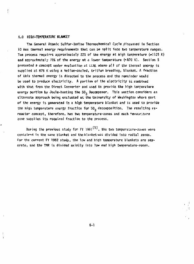
6.0 HIGH-TEMPERATURE BLANKET The General Atomic Sulfur-Iodine Thermochemical Cycle discussed in Section

10 has thermal energy requirements that can be split into two temperature ranges. The process requires approximately 22% of the energy at high temperature {*»1125 K) and approximately 78% of the energy at a lower temperature ("-S70 K). Section S presented a concept under evaluation at LLNL where all of the thermal energy is supplied at 875 K using a helium-cooled, tritium breeding, blanket. A fraction of this thermal energy is directed to the process and the remainder would be used to produce electricity. A portion of the electricity is combined with that from the Direct Converter and used to provide the high temperature energy portion by Joule-heating the SO, Decomposer. This section considers an alternate approach being evaluated at the University of Washington where part of the energy is generated in a high temperature blanket and is used to provide the high temperature energy fraction for SO- decomposition. The resulting re-reactor concept, therefore, has two temperature-zones and each temotruture zone supplies its required fraction to the process.

During the previous study for FY 198r ', the two temperature-zones were contained in the same blanket and the blanket was divided into radial zones. For the current FY 1982 study, the low and high temperature blankets are sep­arate, and the THR is divided axially into low and high temperature-zones.

6-1

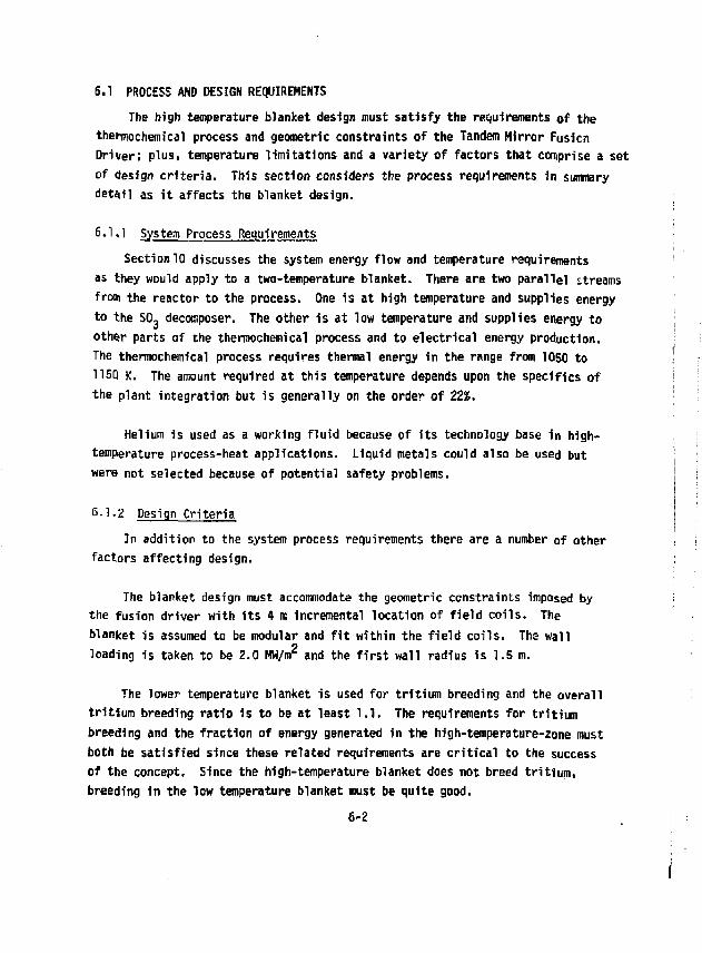
6.1 PROCESS AND DESIGN REQUIREMENTS The high temperature blanket design must satisfy the requirements of the

thermochemical process and geometric constraints of the Tandem Mirror Fusicn Driver; plus, temperature limitations and a variety of factors that comprise a set of design criteria. This section considers the process requirements in summary detail as it affects the blanket design.

6.K1 System Process Requirements Section 10 discusses the system energy flow and temperature requirements

as they would apply to a two-temperature blanket. There are two parallel streams from the reactor to the process. One is at high temperature and supplies energy to the SO- decomposer. The other is at low temperature and supplies energy to oth^r parts of the thermochemical process and to electrical energy production. The thermochemical process requires thermal energy in the range from 1050 to 115Q K. The amount required at this temperature depends upon the specifics of the plant integration but is generally on the order of 22%.

Helium is used as a working fluid because of its technology base in high-temperature process-heat applications. Liquid metals could also be used but were not selected because of potential safety problems.

6-1.2 Design Criteria In addition to the system process requirements there are a number of other

factors affecting design.

The blanket design must accommodate the geometric constraints imposed by the fusion driver with its 4 m incremental location of field coils. The blanket is assumed to be modular and fit within the field coils. The wall loading is taken to be 2.0 MW/nr and the first wall radius is 1.5 m.

The lower temperature blanket is used for tritium breeding and the overall tritium breeding ratio 1s to be at least 1.1. The requirements for tritium breeding and the fraction of energy generated in the high-temperature-zone must both be satisfied since these related requirements are critical to the success of the concept. Since the high-temperature blanket does not breed tritium, breeding in the low temperature blanket must be quite good.

6-2

The flow rates 1n the process components ire fixed by the process require­ments. The blanket design however must maintain temperatures of the flow and structure to acceptable levels consistent with the performance capability of the materials involved. The flow channel and piping design must also have suf­ficiently low pressure drop. A pressure drop of 0.04 of the absolute helium pressure is a typical limit for high temperature helium loops.

6-3

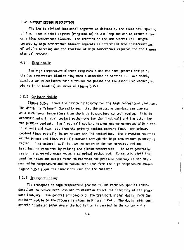
6.2 SWWARY DESIGN DESCRIPTION The TMR is divided into axial segments as defined by the field coil spacing

of 4 m. Each blanked segment (ring module} is 2 m long and can be either a low or a high temperature blanket. The fraction of the THR central cell length covered by high temperature blanket segments is determined from

considerations of tritium breeding and the fraction of high temperature required for the thermo-chemical process. 6.2.1 ftjng Module

The high temperature blanket rir.g module has the same general design as the low temperature blanket ring module described in Section 5. Each module consists of 18 canisters that surround the plasma and the associated connecting piping (ring headers) as shown in Figure 6.2-1.

6.2.2 Canister Module Figtjre 6.2-2 shows the design philosophy for the high temperature canister.

The design is "staged" thermally such that the pressure boundary can operate at a much lower temperature than the high temperature central region. This is accomplished with dual coolant paths- -one for the first wall and the other "For the primary coolant. The first wall coolant removes energy generated within the first wall and heat lost from the primary coolant entrant flow. The primary coolant flows radially inward toward the TMR centerline. The direction reverses at the plenum and flows radially outward through the high temperature generating region, A structural wall is used to separate the two streairs; and any heat loss is recovered by raising the plenum temperature. The heat generating region is currently taken to be a spherical packed bed. Concentric pipes at-e

used for inlet and outlet flows to jnainlaiji the pressure boundary at the mirri-mum helium temperature and to reduce heat loss from the high temperature str e am. Figure 6.2-3 shows the dimensions used for the canister.

6.2.3 Tj-ansport Piping The transport of high temperature process fluids requires special consi­

deration? to reduce heat loss and to maintain structural integrity of the pres­sure boundary. The general philosophy of the transport piping design from the canister module to the process is shown in Figure 6.2-4 . The design uses con­centric insulated pipes where the hot helium is carried in the center and a

6-4

INLET EJIIT FLOW FLOW

EXIT PLENUM EXIT PLENUM

HEAT GENERATING POROUS EED

SECTIOH AT IHIFT PIPE SECTION AT EXIT PIPE

SHIELD

EXIT PLENUM

CORE

INLET PLENUM —- FIRST WALL

Figure 6.2-3 Principal dimensions of the high temperature blanket canister. 6-7

INSULATION OUTER PIPE £ PRESSURE BOUND

INNER PIPE 'INSULATION HELIUM COOLING

A •

•ii

Figure 6.2-4 Higti temperature helium transport pipe,

6-8

coolant is carried in the outer annuius. The helium coolant maintains the outer pressure boundary at a moderate temperature to assure strength. Heat loss from the transported helium is kept small by the internal insulation. Pressure balancing between the two helium streams relieves the stress load on the inner pipe and insulation.

6-9

6.3 NEUTRONICS AHALYSIS

An alternative to the joule boosted concept where the high temperature heat for the decomposer is produced electrically is a two zone blanket design where the high temperature heat is produced directly in the blanket. This can be accomplished by either radial or axial zoning. An axial-zoned system divides the blanket axially into a high temperature blanket, which usually does not produce tritium (in order to avoid difficulties with tritium production and control at high temperatures), and a low temperature blanket. The low tempera­ture blanket is required to breed tritium at a rate that is adequate to fuel the entire reactor (see Figure 6.3-1). A radially zoned blanket consists of only one type of blanket, and divides the tritium breeding and high temperature functions radially, with the tritium breeding region usually being located near the first wall, and the high temperature region in the outer portion of the blanket.

A primary concern associated with any two zone blanket design, whether axial or radial, is the tradeoff between tritium breeding and the fraction of energy deposited in the high temperature zone. In the previous year's work the feasibility of a radially zoned blanket was examined.^ ' This design has been replaced by the axially zoned concept depicted in Figure 3.3-1. This type of design faces many of the same problems as the radially zoned blanket but could result in a less complicated design. In this section are described the neutronics analyses of the high temperature modules for the axially zoned blanket design.

The neutronics calculations for these analyses have been performed with the Oct. 1980 version of the one dimensional discrete ordinates transport code ONEDANT.^ ' This code is described in more detail in Section 5.5.

6.3.1 Energy Split and Tritium Breeding

In an axially zoned blanket design, the fraction of heat produced in a high temperature, F„, is dependent upon several variables: TBR, the tritium breeding ratio; ft, and M, , the high and low temperature zone blanket energy

6-10

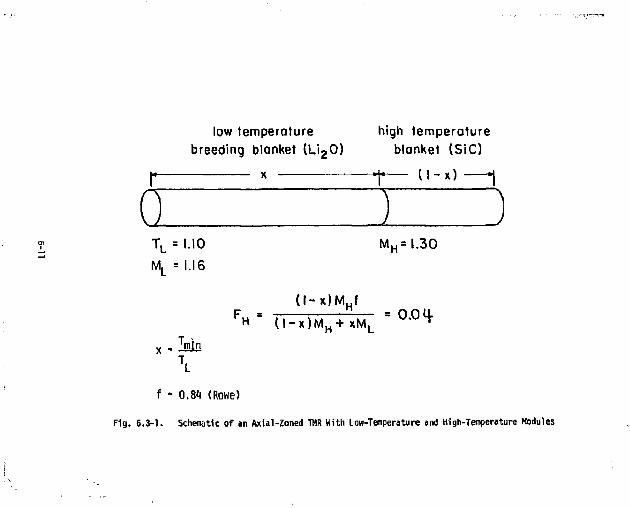
low temperature high temperature breeding blanket ( L i 2 0 ) blanket CSiC)

l l - x ) 1 a i T L = 1.10 M L = 1.16

M H = I . 30

( l - x ) M H f H ( l - x ) M H + x M L

0.0 q-

min

f - 0.81 (Rowe)

Fig. 6.3-1. Schematic of an Axial-Zoned TMR With Low-Temperature and High-Temperature Modules

multiplication factors; f, the fraction of heat deposited in the high tempera­ture zone and recovered at high temperature. Figure 6.3-2 illustrates the relationship between these factors. The overall breeding, TBR, is equal to the breeding ratio in the breeding region, denoted by T L > times the fraction of the overall length devoted to the breeding region, denoted by x. Since the dominant constraint is a value of 1.1 for TBR, once T. is determined the value of x becomes fixed as shown in the single curve for the right ordinate in Figure 6.3-2. Obviously,higher values of T. permit the use of shorter frac­tional lengths of the breeding region. Similarly, F„ is then also determined using the equation shown in Figure 6.3-1. The family of curves in Figure 6.3-Z show that F H increases with both increasing values of T L (because a greater fraction of the length can be devoted to high temperature operation) and M„ (because more energy is being deposited in the high temperature blanket).

The reference high temperature blanket design is the silicon carbide module design described in Section 6.1. Two other high temperature blankets were also analyzed neutronically, a helium cooled aluminum oxide blanket similar to the silicon carbide blanket, and a sodium cooled blanket with TZH structure. The results of all three designs are presented in Table 6.3-1.

The silicon carbide and aluminum oxide designs have similar results with the latter producing a higher energy multiplication factor. Neutronically, the TZM/Na design is superior to both, with a higher energy multiplication factor and mucjuhigher f value. The higher f value is a consequence of the assumption that a separate first wall cooling system would not be required for this sys­tem. These neutronics advantages must, of course, be weighted against the dis­advantages of a Na-cooled design, including safety and HHD pressure drop. There are also advantages to a SiC design in terms of materials properties.

Several axial zoning blanket combinations are listed in Table 6.3-2. The current value required for F„ is approximately 25 to 3055, which implies that the tritium breeding ratio in the low temperature blanket must be in the 1.4 to 1.5 range. The initial reference low temperature blanket design had a breeding ratio of only 1.1. The results given in Table 6.3-2 show that while such a design can breed adequately for a one zone joule boosted concept,

6-12

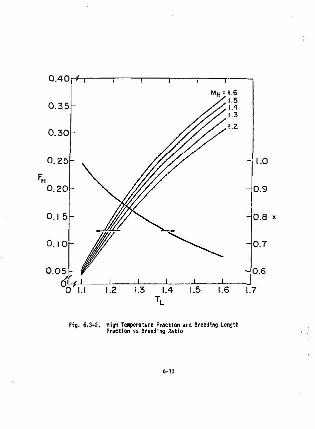
0.40

0.35

0.30

' \ 1 1 I l l -

M H = | .6 JS 1.5

— yy,\A / / / { 3

/ / / / \ ! , 2

Fig. 6.3-Z. High Temperature Fraction and Breeding Length Fraction vs Breeding Ratio

6-13

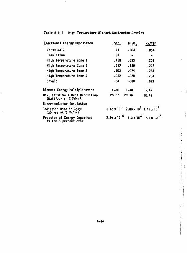
Table 6.3-1 High Temperature Blanket Neutron!cs Results

Fractional Energy Deposition First Wall Insulation High Temperature Zone 1 High Temperature Zone 2 High Temperature Zone 3 High Temperature Zone 4 Shield

Blanket Energy Multiplication Max. First Wall Heat Deposition

(Watt/cc - at. 2 MW/m2) Superconductor Insulation Radiation Dose in Grays

(30 yrs at 2 MW/m2) Fraction of Energy Deposited

In the Superconductor

S.lc. MA- Ha/TZH

.11 .063 .034

.01 - -.468 .633 .206 .217 .189 .225 .103 .074 .253 .052 .028 .261 .04 .008 .021

1.30 1.40 1.47 25.27 29.16 25.49

3.66 x lO 8 2.88x 107 3.47:<107

7.96xlO' 6 6.3xl0" 7 7.1x10"

6-14

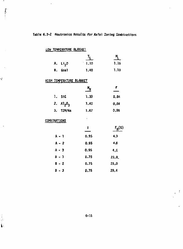
Table 6.3-2 Neutxonics Results for Axfal Zonfng Combinations

LOW TEMPERATURE BLANKET

JL A. A. L i 2 0 1.10 1.16

B. Goal 1.40 1.10

HIGH TEMPERATURE BLANKET

A f

1 . SiC 1.30 0.84

2 . A J 2 0 3 1.40 0.84

3. TZM/Na 1.47 0.96

COMBINATIONS

X FH(X]

A • 1 0.95 43

A - 2 0.95 4.6

A - 3 0.95 4.6

B - 1 0.75 23.8 .

B - 2 0.75 25,0

B - 3 0,75 29,4

6-15

Li

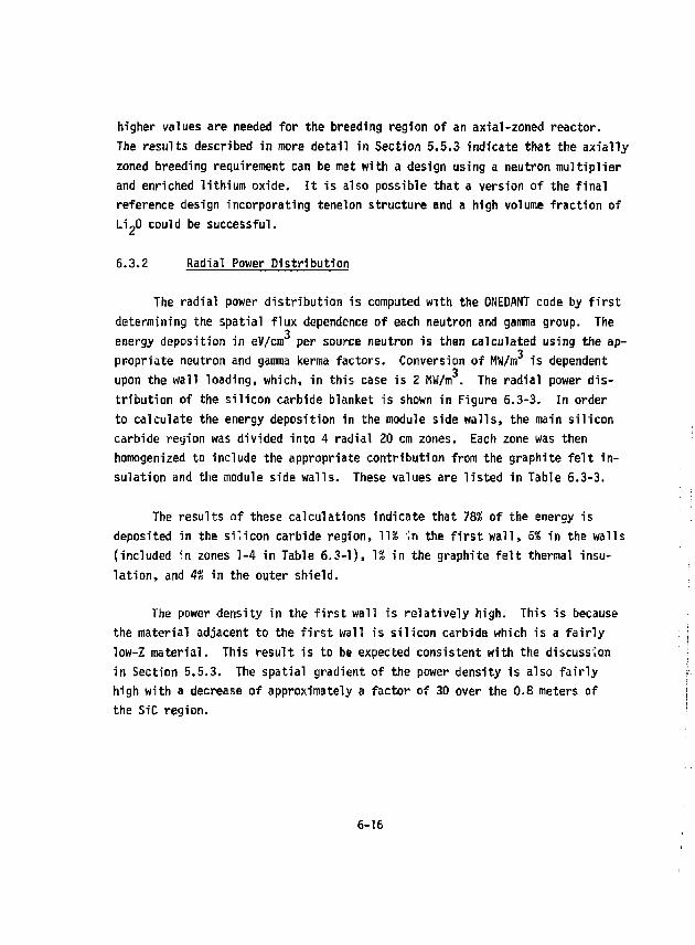
higher values are needed for the breeding region of an axial-zoned reactor. The results described in more detail in Section 5.5.3 indicate that the axially zoned breeding requirement can be met with a design using a neutron multiplier and enriched lithium oxide. It is also possible that a version of the final reference design incorporating tenelon structure and a high volume fraction of Li~0 could be successful.

6.3.2 Radial Power Distribution

The radial power distribution is computed with the ONEDANT code by first determining the spatial flux dependence of each neutron and gamma group. The 3 energy deposition in eV/cm per source neutron is then calculated using the ap-3 propriate neutron and gamma kerma factors. Conversion of HW/m is dependent

3 upon the wall loading, which, in this case is 2 MW/m . The radial power dis­tribution of the silicon carbide blanket is shown in Figure 6.3-3. In order to calculate the energy deposition in the module side walls, the main silicon carbide region was divided into 4 radial 20 cm zones. Each zone was then homogenized to include the appropriate contribution from the graphite felt in­sulation and the module side walls. These values are listed in Table 6.3-3.

The results of these calculations indicate that 78% of the energy is deposited in the silicon carbide region, "\~\% !n the first wall, 5% in the walls (included in zones 1-4 in Table 6.3-1), 1£ in the graphite felt thermal insu­lation, and 4% in the outer shield.

The power density in the first wall is relatively high. This is because the material adjacent to the first wall is silicon carbide which is a fairly low-Z material. This result is to be expected consistent with the discussion in Section 5.5.3. The spatial gradient of the power density is also fairly high with a decrease of approximately a factor of 30 over the 0.8 meters of the SiC region.

6-16

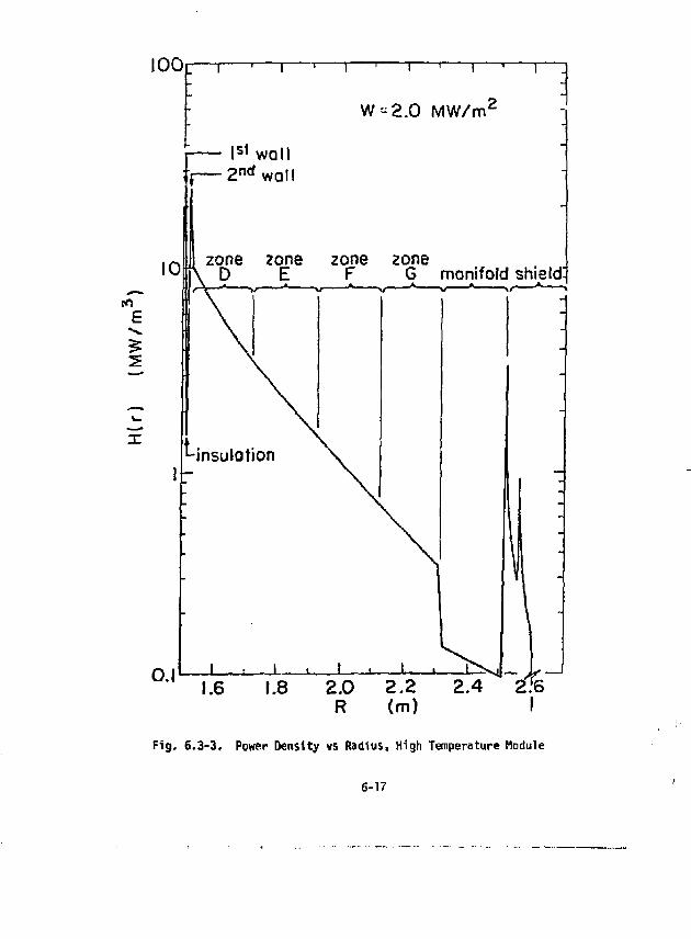
100

to

W-2.0 MW/m 2

I s 1 WQI 2 n d WQ

zone zone zone zone D E F 6 manifold shield:

Fig, 6.3-3, Power Density vs Radius, High Temperature Module

6-17

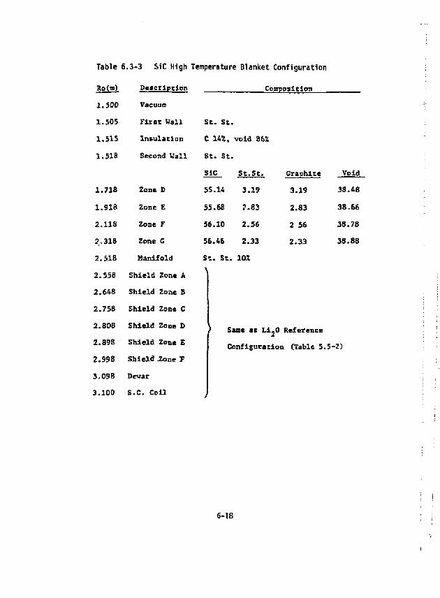
Table 6.3-3 SiC High Temperature Blanket Configuration

Ro(ffl) Description

Vacuum

Coop ssitlon

2.500

Description

Vacuum

1.505 Firet Hall St. St.

1.515 Insulation C 14X, void 86%

1.518 Second Vail St. St.

SiC St.St. Graphite Void

1.718 Zone D 55.14 3.19 3.19 38.48

1.918 Zone E 55.68 ?-83 2.83 38.66

2.IIS Zone F 56.10 2.56 2 56 38.78

2,318 Zone G 56.46 2.33 2.33 38.88

2.518 Manifold St. St. 102

2.558 Shield Zone A \

2.648 Shield Zone B

2.758 Shield Zone C

2.808 Shield Zone D * Same as Li.O Reference 2.898 Shield Zone £ Configuration (Table 5.5-2) 2.998 Shield .Zone T

3.09B Devar

3.100 S.C. Coil i

6-18

6.3.3 Radiation Damage

Table 6.3-1 listed the values of the superconducting insulation radiation dose and the fraction of heat deposited in the coil and dewar system. The values for the silicon carbide blanket are quite high, mainly due to the fact that silicon carbide is not a very good shielding material. Based on a limit of 5x10 grays, the insulation would only have a 4 year lifetime. An addi­tional 20 cm of shielding will probably be required in order to reduce the re­frigeration power requirements and increase the insulation lifetime of accept­able values.

A general discussion of the parameters relevant to radiation damage and the limitations considered acceptable is included in Section 5.5.2.

6.3.4 Neutronics Conclusions

Axial zoning is an attractive option for a fusion reactor designed to produce high temperature heat for a synfuel plant. The physical separation of the high temperature energy recovery, and the tritium breeding has the virtues of blanket module simplicity (and, therefore, probably reliability), and more efficient use of space (and, therefore, smaller field coils and lower cost) by requiring only one cooling system per module. Any radial-zoned system is likely to suffer by comparison in these respects.

The high temperature module analysed in this work appears to be a cred­ible approach in terms of neutronics performance. It must, however, be coupled with a low temperature module which can produce a tritium breeding ratio;? 1.4. Of the options considered thus far, the most promising appears to be a Li 20 design with a lead-zirconate multiplier as described in Section 5.5.3.

6-19

6.4 BLANKET THERMAL-HYDRAULIC ANALYSIS The thermal-hydraulic analysis is concerned with the calculation of:

1) coolant and structural temperature; 2) heat loss from the high temperature stream; and 3) pressure drop through various flow paths. The analysis was performed by using an analytical model that considers the baste heat transfer and flow processes within the canister.

The heat transfer processes considered are shown in Figure 6,4-1. Thermal energy generated within the first wall structure is transferred to the first wall coolant stream. There is also heat transferred to the first wall coolant from the energy generated within the insulating wall and from heat lost through that wall from the primary coolant inlet stream. The energy transferred to the first wall coolant is lost from the high temperature zone but can be used for lower temperature energy loads. Energy generated within the core is transferred to the primary coolant which is h-iated to its maximum temperature at its exit from the core. There is some heat loss from the core region to the inlet flow because of the temperature difference. There is also t ansfer of energy gene­rated in the core wall to inlet flow. Those heat transfers are not lost but only increase the inlet temperature enroute to the inlet plenum. The analytical model uses simplified thermal energy balances ^nd heat transfers based on key temperatures.

Pressure drop through various components of the coolant paths are computed based upon the results of the thermal analysis, in general the analysis starts with a set of given temperatures (in and out) and the module power from which Che flow rate is calculated. The flow rate is used to define coolant velocity, heat transfers and friction coefficients.

The following discussion presents additions'; details 3f the analysis for the first wall and high temperature region.

6.4.1 First Hall Analysis The first wall is assummed to be adiabatic (no heat transfer) t its outer

surface so all generated energy flows through the inner surface to the first wall coolant. The resulting temperature of the first wall therefore exceeds

6-20

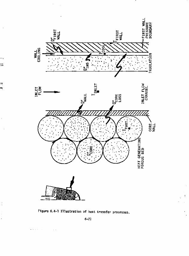
Figure 6.4-1 Illustration of heat transfer processes. 6-21

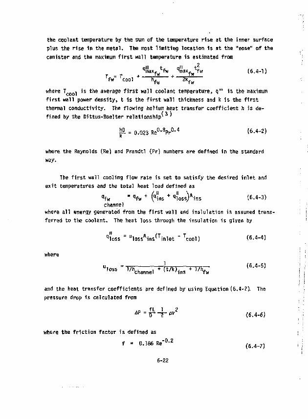
the coolant temperature by the sum of the temperature rise at the inner surface plus the rise in the metal. The most limiting location is at the "nose" of the canister and the maximum first wall temperature is estimated from

"max^fw qjn'ax^fw (6.4-1) V Tcool + h f w

+ Z k f w

where T c o o l is the average first wall coolant temperature, q'" is the maximum first wall power density, t is the first wall thickness and k is the first thermal conductivity. The flowing helium heat transfer coefficient h is de­fined by the Dittus-Boelter relationship^ '

f = 0.023 Re°- 8Pr 0- 4 (6-4-2)

where the Reynolds (Re) and Prandtl (Pr) numbers are defined in the standard way.

The first wall cooling flow rate is set to satisfy the desired inlet and exit temperatures and the total heat load defined as

qfw = qfw + (qins + «loss)Ains (6.4-3) channel

where all energy generated from the first wall and inslulation is assumed trans­ferred to the coolant. The heat loss through the insulation is given by

qloss = uloss Ains f Tinlet " Tcool) (6.4-4)

where U ' ° " = ^channel + ^ > i n s + »"£ ^

and the heat transfer coefficients are defined by using Equation (6.4-2). The pressure drop is calculated from

.„ fL 1 2 AP'TT^rev (6.4-6)

where the f r i c t i on factor is defined as

f = 0.186 Re" 0 " 2

( 6 4 _ ; )

6-22

to represent friction factor in smooth channels' . The flow channel thick­ness Is selected to maintain an acceptably low pressure drop.

The various parameters used for the first wall calculations are summarized in Table 6.4-1 and the results are in Table 6.4-2 . The important results are as follows; 1) A first wall temperature of 835 K located at the "nose" of the canister.

This is 67 K above the average coolant temperature of 775 K. 2) A channel width of 3 mm gives a pressure drop of 0.56 atm. With an absolute

pressure of 50 atm, this gives AP/P = 0.011 which is acceptable. 3) The fraction of high temperature module energy lost to the first wall

coolant is 0.12 plus 0,04 loss to the shield giving a total high temperature zone energy loss fraction of 0.16.

6.4.2 High Temperature Region The primary inlet flow is heated enroute to the plenum. The plenum tem­

perature is given by Tplen = Tinlet + Hcore + W e Twal! + qloss Ains (6.4-8) \wall loss/

All energy generated in the core wall is assumed to be transferred to the inlet flow. The heat transfer through the wall is defined analogously to Equation 6.4-4 but with an assumed high heat transfer at the inner core wall.

All energy generated within the core is transferred to the primary coolant. This heats the coolant from the inlet plenum temperature to the exit temperature which is calculated from

Texit = Tplen + qcoreAcore " qcoreAwall (6.4-9) loss

Adding Equations (6.4-8) and (6.4-9) gives

T e * i t = T i n l e t + «corAore " " l o s s e s (6.4-10)

6-23

which indicates that the heat loss through the insulation is the net loss from the high temperature region. The primary flow rate is adjusted iteratively to match the desired inlet and outlet temperature and heat loss.

The core is assumed to consist of a bed of spherical particles. The tem­perature rise to the center of a particle can be calculated from

The spheres are assumed to have a porosity (£) of 0.4 and a thermal conduc­tivity of 25 W/m-k which is typical of Silicon Carbide. The heat transfer coefficient

i 5 \ for a bed of spheres is estimated from the Denton1 ' relationship given by filTD 0 7r. 0 333 (6.4-12} K p

where particle diameter D is used for the characteristic dimension. At the maximum power density near the core inlet> Equation {6.4-11} gives a particle temperature rise of 29 K. At the average power density of the particle the tem­perature rise is 15K. The maximum core temperature is estimated at 1175 K.

The pressure drop along the primary core coolant path has several major components: inlet and outlet nczzles, inlet channel and spherical particle bed. The flow areas of those components were sized such that A?/? $ o.oi.

The pressure drop through the nozzles was calculated using pressure loss coefficients of 2.0 each. The pressure drop through the inlet channel was calculated using the friction factor defined by Equation C6.4-7Jplus a plenum pressure loss coefficient of 1.0.

The pressure drop through the packed bed of the spheres was calculated by using

Ap = 1 K pv 2 (6.4-13) core 2 core M

6-24

v.i re v is the velocity based on the core flow area without spheres. K I c\ core

was calculated from the Ergun* 3 ; relationship ^re'^^f'^ 1 5 0 ^ ] (6-4.14)

where £ is the porosity (0.40).

A summary of selected parameters used for high temperature region calcu­lations is summarized in Table 6.4-1 and the results are presented in Table 6.4-2 . The important results are as follows: 1) The maximum spherical particle temperature is estimated to be 1175 K based

on core average power density and exit plenum temperature. (The particle diameter is 15 mm based on thermal stress considerations).

2) The core wall thickness of 3 mm is sufficiently thin to keep its tempera­ture midway between the inlet and exit temperature.

3} The fraction of the core energy lost through the insulation to the first wall coolant is 0.04.

4) The most limiting pressure drop components are the inlet and outlet nozzles. The pressure drop there is responsible for the primary coolant pressure of 50 atm.

6-25

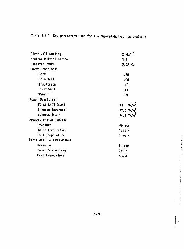
Table 6.4-1 Key parameters used for the thermal-hydraulics analysi

First Wall Loading Neutron Multiplication Canister Power Power Fractions:

Core Core Wall Insultaion First WaTT Shield

t'ower Densities: First Wall (max) Spheres (average) Spheres (max)

Primary Helium Coolant Pressure Inlet Temperature Exit Temperature

f:irst Wall Helium Coolant Pressure Inlet Temperature Exit 7mper3ti/re

2 HW/mZ

1.3 2.72 HW

.78

.06

.01

.TI

.04

18 HW/m3

17.5 MW/m3

34.1 HW/m3

50 atm 1040 K 1160 K

50 atm 750 K SWX

6-26

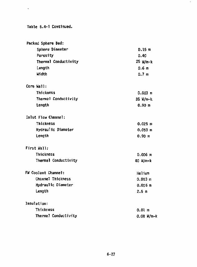
Table 6.4-1 Continued.

Packed Sphere Bed: Sphere Diameter Porosi ty Thermal Conductivity Length Width

Core Wall: Thickness Thermal Conductivity Length

Inlet Flow Channel: Thickness Hydraulic Diameter Length

First Wall: Thickness Thermal Conductivity

FW Coolant Channel: Channel Thickness Hydraulic Diameter Length

Insulation: Thickness Thermal Conductivity

0.15 m 0.40

25 W/m-k 0.6 m 0.7 m

0.003 m 35 Vl/m-k

0.90 m

0.025 m O.050 m 0.90 m

0.006 tn 40 W/m-k

Helium 0.003 m 0.006 m 2.5 m

0.01 m 0.08 W/m-k

6-27

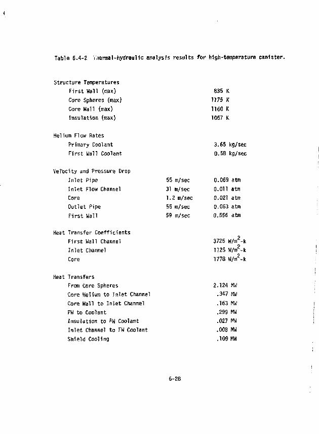
Table 6.4-2 V.iermal-hydraulic analysis results for high-temperature canister.

Structure Temperatures First Wall (max) 835 K Core Spheres (max) 1775 K Core Wall (max) 1160 K Insulation (max) 1067 K

Helium Flow Rates Primary Coolant 3.65 kg/sec First Wall Coolant 0.58 kg/sec

Vel'ocity and Pressure Drop Inlet Pipe 55 m/sec 0.069 atm Inlet Flow Channel 31 m/sec 0.011 atm Core 1.2 m/sec 0.O21 atm Outlet Pipe 55 m/sec 0.063 atm First Wall 59 m/sec 0.556 atm

Heat Transfer Coefficients First Wall Channel 3725 W/m 2-k Inlet Channel 1125 W/m^k Core 1778 W/m 2-k

Heat Transfers From Core Spheres 2.124 MW Core Helium to Inlet Channel .347 MW Core Wall to Inlet Channel .163 MW FW to Coolant .299 MW Insulation to FW Coolant .027 m Inlet Channel to FW Coolant .008 MW Shield Cooling .109 MW

6-28

6.5 STRESS ANALYSIS Stress analysis was performed to assure reasonable sizing of the first

wall thickness for pressure containment and to size the core spheres based on thermally induced stresses. Additional discussion of canister module stresses is incTuded in Section 5.0.

6.5.1 First Hall First wall hoop Stress was calculated to help determine the required thick­

ness of the first wall. It is desired to have a thin first wall to reduce tem­peratures out a thick wall for strength. The circumferential hoop stress at the "nose" of the canister is most limiting and can be calculated by^ '

«t-T-< p1-V where {P- - P ) is the pressure difference (50 atm), R is the radius of curva­ture (0.13 m) and t is the thickness (0.006 m). The resulting stress of 110 MPa (13000 psi) is reasonable.

6.5.2 Core Spheres

Each sphere in the core will have thermal stresses because of the radial temperature gradients existing in each sphere. The inside of the sphere is hotter than the outside so, the differential expansion causes compressive stress at the inside and tensile stress at the outside. Tne maximum tensile stress at the surface of the sphere at the maximum power density is limiting and can be calculated from* '

_ aE 2ql"R2

°t max " T^~v 30lT

The property values used are a = 26 x 10" 6, v = 0.3, k = 25 W/m-k, R = 0.007b m, E = 1.38 x 10 5 MPa, q'" = 16.6 HW/m3 and result in a stress of 12.8 MPa (1854 psi).

6.5.3 Other Considerations There are additional stress considerations important to the canister design.

These are primarily concerned with the stresses in the pressure boundary of the canister. Each canister is considered to be self supportive of its neighbor.

6-29

This works well for the flat surfaces of canisters in a ring because depres-surization in one would lead to simultaneous depressurization in the others. There could be a problem with the ends, however, depending upon the degree of axial isolation of each ring module. Stresses in these end regions have not been considered for the high temperature canister.

While the pressure boundary (first wall) is cooled, there are temperature gradients that would lead to thermal stresses. This is of most concern for the rather large flat panels making up each canister and at the corner joints. These thermal stresses have not been considered in the present analysis. These have been considered in Section 5.2.

6-30

6.6 HIGH TEMPERATUftE BLANKET CONCLUSIONS The following conclusions can be made regarding the high temperature

blanket: t The high temperature blanket provides a direct replacement (geometrically)

for the low temperature tritium-breeding, blanket presented in Section 5. • Since the high temperature blanket does not breed tritium, the low temp­

erature blanket must be a high breeder for the overall breeding ratio to be £ 1.1.

• Absolute helium pressure of about 50 a tin is necessary to maintain acceptable pressure drop.

• The system pressure is contained within the specially cooled first wall (pressure boundary) and helium transport piping. (The heat exchanger tubes of the fluidized bed decomposer must also contain system pressure and at high temperature).

• First wall (pressure boundary) cooling can maintain the structural temp­eratures at levels consistent with the low temperature blanket. The high temperature internal structure and components only need to be self sup­porting.

• Heat transfer within the blanket is quite good and can maintain component temperatures at less than 1175 K. The coolant exit temperature is 1160 K.

• Structural and mechanical design issues need further development and study— especially mechanical and thermal stress analysis. Many of these issues are common to both the low and high temperature blanket canister modules.

6-31

References for Section 6.0

7. R. W. Werner, et. al., Synefuels. from Fusion - Using the Tandem Mirror Reactor and a Thermochemical Cycle to Produce Hydrogen, UCID-19311, Lawrence Livemrore Laboratory (February 9, 1982).

2. T. R. Hill, "ONETRAN" ft Discrete Ordinates Finite Element Code for the Solution of the One-Dimensional Multigroup Transport Equation," LA-5900-MS, Los Alamos Scientific Laboratory (June 1975). (The pre-release availability of ONEDANT to the study fs a result of the courtesy of Oonald J. Dudziak of Group T-l, Los Alamos Scientific Laboratory.)

3. J. P. Holman, Heat Transfer, (McGraw-Hill, N.Y., 1976). 4. H. Rouse, Elementary Mechanics of Fluids, John Wiley & Sons, (1946). 5. E. R. G. Eckert and R. M. Drake, Jr., Heat and Mass Transfer, Second Edition.

McGraw Hill (1959). 6. E. P, Popov, Mechanics of Materials, Prentice-Hall (1952). 7. S. P, Timoshenko and J. N. Goodier, Theory of Elasticity, Third Edition,

McGraw Hill (1970).

6-3E

SECTION 7 ENERGY TRANSPORT SYSTEM - REACTOR TO PROCESS

Contributor: R. W. Werner

TABLE OF CONTENTS Section Page 7.0 ENERGY TRANSPORT SYSTEM - REACTOR TO PROCESS 7-1 7.1 OBJECTIVES AND SAFETY CONSTRAINTS 7-1 7.2 ENGINEERING OPTIONS 7-2 7.3 CASE STUDIES 7-2 7.4 CYCLE EFFICIENCY AND PLANT AVAILABILITY 7-4 7.5 HELIUM PIPING OPTIMIZATION STUDIES 7-4 7.6 CONCLUSIONS ON ENERGY TRANSPORT 7-5

REFERENCES 7-6

1

Ja

7.0 ENERGY TRANSPORT SYSTEM - REACTOR TO PROCESS

The two reactor blanket designs discussed in Sections 5 and 6 provide energy for the General Atomic Sulfur-Iodine Thermochemical Cycle in two different ways and in two different temperature ranges. The first, the Canister blanket discussed in Section 5, produces 825 K process heat for the bulk (78%) of the thermochemical plant needs, while the S0 3 decomposer, which is the high temperature demand part of the cycle, is driven electri­cally using the Joule-Boosted SO, Decomposer. The second, the Axial Two-Zone blanket described in Section 6, provides both high temperature thermal energy {1160 K) for the top end of the plant and 825 ' process heat for the remainder of the plant.

This section discussed the options and alternatives available for trans­porting this energy to the chemical plant. System evaluations addressing both the problems of matching heat source to heat sink and designing for safe energy transport have been studied. The ti insport system selected for both blanket designs uses helium as the heat transport fluid.

7.1 OBJECTIVES AND SAFETY CONSTRAINTS

Both blanket concepts, the Canister blanket and the Axial Two-Zone blanket, must deliver heat at the appropriate amounts and temperatures to the chemical plant in order to achieve an overall efficient and economic process. The majority of the chemical engineering effort in this project has been devo+pH to developing techniques of matching the heat source to the heat demands of the process and then developing process unit designs that can effectively and economically make use of this heat profile.

Safety considerations have been an integral part of the chemical engi­neering. Attention tc potential problems in liquid metal safety, helium coolant over-pressuring of process vessels, tritium permeation and contamin­ation, and migration of neutron-activated corrosion products are some of these safety considerations.

7-1

7.2 ENGINEERING OPTIONS

A very large number of engineering approaches for matching the heat source to the heat demands of the chemical process were examined in order to identify those which met the following desired characteristics:

o The majority of piping for long-distance heat transport within the chemical plant shall use high quality steam.

o Liquid metal coolants shall not be used within the chemical plant.

o Piping distances of high pressure helium piping shall be minimized to reduce pumping power.

o Multiple barrier isolation shall be provided between the neutron-activated blanket materials and the hydrogen product,

o Highly redundant modularity shall be used whenever possible to increase plant availability and reduce the quantity of neutron-activated materials that could be accidently released.

7.3 CASE STUDIES

Space does not permit us to outline in detail the large number of case studies that were made in order to select and design a blanket process inter­face and then evaluate its performance. Some of these cases have been covered in earlier papers* ' and prior year's reports/ *5' Both he and Na were considered for heat transport in the process in FY80, and were coupled with steam-Rankine cycles for electrical power generation. Only He was used in FY81 and this year for heat transport out of the blanket. Various cycles were evaluated for electrical power generation, i.e., steam-Rankine, steam-Freon, steam-ammonia, and Brayton-steam in FY81. In FY32 we used the steam-Rankine exclusively in cur study.

7-2

The TMR 0 was parametrically varied from 10 to 35. In the resultant cases, there were blanket temperatures or process conditions that needed to be varied. The following approaches were investigated:

0 Heat pipe blanket (He) 800 - 1150 K o Heat pipe blanket (Na) 800 - 1150 K o Two-zone blanket:

Low temperature (He) 800 - 950 K High temperature (He) 900 - 1150 K

o First wall (Na or He) 700 - 850 K O Direct convertor Hx (He) 850 - 1050 K System evaluations were made for these approaches by attempting to match

the heat source to the process heat demand as follows: by developing a heat exchanger network train, by developing electric power generating systems on both topping and bottoming cycles, and by roughly optimizing the network and then evaluating the thermal efficiency. For cases involving helium-Brayton turbine cycles, each of these helium loops had to be optimized with a small computer program by varying temperatures, He flow rates and turbine wheel compression ratios. The loops were linked and the network system optimized factorily. This tedious process was required to produce the best set of temperatures, helium flows, and heat exchanger match-ups consistent with the highest efficiency. Thermal efficiency ranged from 32 to SB% for the thermo-chemical process depending mainly upon the particular selection of topping and bottoming cycles. As expected, an increase in Q from 10 to 35 also gave an increase in process efficiency (up to an incremental gain of -v. 4%) because of the increased availability of electricity at a high conversion efficiency from the direct convertor. In our FY82 studies, the helium-Brayton turbine cycles were abandoned in favor of a steam cycle with an intermediate heat exchanger containing the helium coolant in the primary loop.

7-3

7.4 CVCLE EFFICIENCY AND PLANT AVAILABILITY

He have explored the variation of cycle efficiency with changes in the energy transport system and coupling of the blanket to the process. Gener­ally, we found high cycle efficiency was obtained when liquid sodium was used to generate steam and drive process units. But we felt that liquid metal coolants also provided a serious fire and safety risk which would result in a reduction in total plant availability. The damage consequences from accidents could be severe.

High pressure helium was found to have the disadvantages of poor heat transfer (and thus large temperature gradients within the heat transfer equipment), significant pumping power, and the hazards associated with high pressure. Helium coupling generally produced higher plant availability than with liquid metal heat transport. We conclude that the safety and avail­ability advantages of helium make it the preferred heat transport fluid.

7.5 HELIUM PIPING OPTIMIZATION STUDIES

In carrying out the case studies, it became clear that although helium had clear safety and operational advantages, there were also clear economic debits in terms of pumping power and high pressure equipment capital costs. Therefore, a tradeoff study was done between capital costs and operational pumping power costs. The details of this rough optimization study were reported earlier/ ' For heavy wall Inr loy-SOOH piping, using a perforated liner to help keep the outer wall cooler, the minimum total operating and amortized capital cost was found for a 2-m-diameter, 100-m-long, 1.0 MPa pressure, 7-pipe transfer system feeding a helium-heated decomposer or boiler using blanket heat. The minimum cost was around J35M--somewhat high.

After this earlier study, we developed a design using Kao-Wool insula­tion' ' in place of the stagnant helium gap between the perforated liner and the heavy outer wall. This more effective insulation allowed us to drop the outer wall temperature so that mild steel would be acceptable (i.e., IX

7-4

creep in -v, 20 years) and allow the helium pressures to be increased to 3.0 MPa. This improvement dropped the total operating and amortized capital cost to about J10M--a substantial improvement.

7.6 CONCLUSIONS ON ENERGY TRANSPORT

In this section we have outlined the range of transport system altera­tives that were examined in developing a design concept that employs a helium-steam-Rankine cycle approach. This satisfies our desire to achieve good isolation of the chemical plant from radioactivity by using helium coolants, and to substitute for liquid sodium the more conventional process steam approach to driving the chemical plant.

7-5

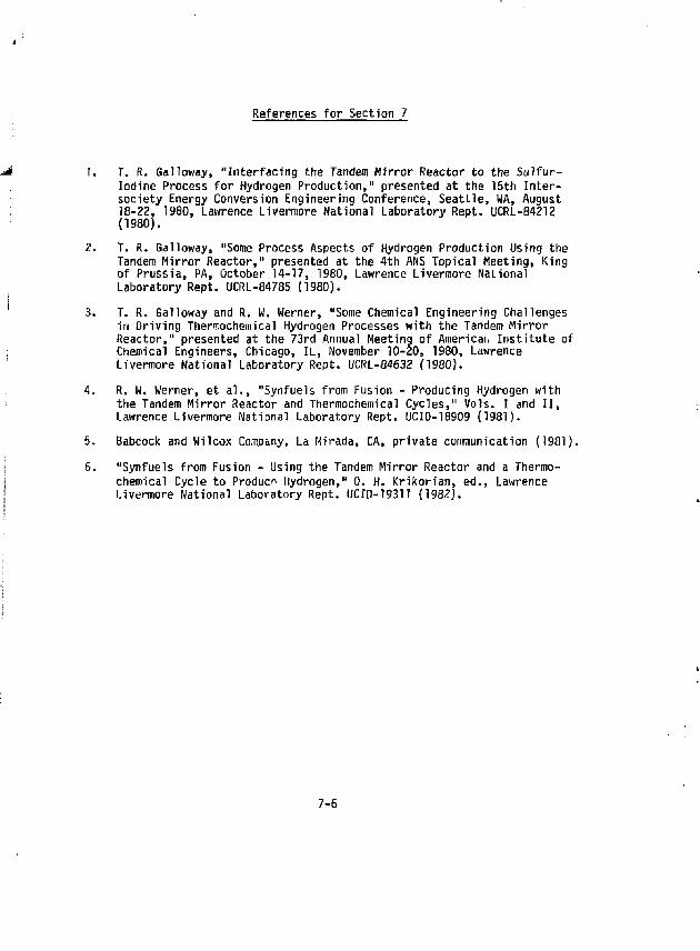
References for Section 7

1. T. R. Galloway, "Interfacing the Tandem Mirror Reactor to the Sulfur-Iodine Process for Hydrogen Production," presented at the 15th Inter-society Energy Conversion Engineering Conference, Seattle, WA, August 18-22, 1980, Lawrence Livermore National Laboratory Rept. UCRL-84212 (1980).

2. T. R. Galloway, "Some Process Aspects of Hydrogen Production Using the Tandem Mirror Reactor," presented at the 4th ANS Topical Meeting, King of Prussia, PA, October 14-17, 1980, Lawrence Livermore National Laboratory Rept. UCRL-84785 (1980).

3. T. R. Galloway and R. w. Werner, "Some Chemical Engineering Challenges in Driving Thermochemical Hydrogen Processes with the Tandem Mirror Reactor," presented at the 73rd Annual Meeting of American Institute of Chemical Engineers, Chicago, IL, November 10-20, 1980, Lawrence Livermore National Laboratory Rept. UCRL-84632 (1980).

4. R. W. Werner, et al., "Synfuels from Fusion - Producing Hydrogen with the Tandem Mirror Reactor and Thermochemical Cycles," Vols. I and II, Lawrence Livermore National Laboratory Rept. UCID-18909 (1981).

5. Babcock and Wilcox Company, La Mirada, CA, private communication (1981). 6. "Synfuels from Fusion - Using the Tandem Mirror Reactor and a Thermo­

chemical Cycle to Produce Hydrogen," 0. H. Krikorian, ed., Lawrence Livermore National Laboratory Rept. l/CIO-19311 (1982).

7-6

SECTION 8 THERMOCHEHICAL HYDROGEN PROCESSES

Contributor: 0. Krikorian

TABLE OF CONTENTS ion Page THERMOCHEMiCAL HYDROGEN PROCESSES 8-1 BASiL PRINCIPLES OF THERHOCHEHICAL CYCLES 8-1 8.1.1 Introduction 8-1 8.1.2 Basic Principles 8-2 8.1.3 Some Important Criteria 8-6 GENERAL ATOHIC CYCLE 8-8 8.2.1 Selecting a Cycle 8-8 8.2.2 Chemical Description of GA Cycle 8-8 THERMODYNAHIC DATA BASE FOR SECTION II 8-11 B.3.1 Sequence of Process Steps 8-11 8.3.2 Thermodynamic Data Requirements 8-14 8.3.3 Summary of Thermodynamic Data 8-18 REFERENCES . . . . . 8-33

1"

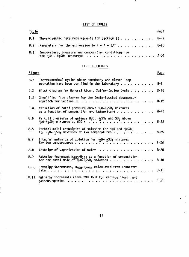
LIST OF TABLES Table Page 8.1 Thermodynamic data requirements for Section II 8-19 8.2 Parameters for the expression In P = A - B/T 8-20 8.3 Temperature, pressure and composition conditions for

the H2O - H2SO4 azeotrope 8-21

LIST OF FIGURES Figure Page 8.1 Thermochemical cycles whose chemistry and closed loop

operation have been verified in the laboratory 8-3 8.2 Block diagram for General Atomic Sulfur-Iodine Cycle 8-10 8.3 Simplified flow diagram for the Joule-Boosted decomposer

approach for Section II 8-12 8.4 Variation of total pressure above H2O-H2SO4 mixtures

as a function of composition and temperature 8-22 8.5 Partial pressures of gaseous H?0, H2SO4 and SO3 above

H 20-H 2S0 4 mixtures at 600 K 8-23 8.6 Partial molal enthalpies of solution for H2O and H2SO4

for H2O-H2SO4 mixtures at two temperatures 8-25 8.7 Integral enthalpy of solution for H2O-H2SO4 mixtures

for two temperatures 8-26 8.8 Enthalpy of vaporization of water 8-28 8.9 Enthalpy increment HgoQ"^298 a s a function of composition

for one total mole of H2O-H2SO4 solution 8-30 8.10 Enthalpy increments, HgoQ-l^gg, calculated from Lennartz'

data 8-31 8.11 Enthalpy increments above 298.15 K for various liquid and

gaseous species 8-32

ii

8.0 THERMOCHEMICAL HYDROGEN PROCESSES

In this section we describe the basic principals of thermocheirricaJ cycles for water splitting to produce hydrogen, including the criteria that determine cycle efficiencies and influence process design. We also describe in a "pry introductory way the Gfl Sulfur-Iodine Cycle for hydrogen production that we are coupling to the TRH in our current design studies.

8.1 BASIC PRINCIPLES OF THERMOCHEMICAL CYCLES

8.1.1 Introduction

A thermochemical cycle for hydrogen production is a process in which water is used as a feedstock along with a non-fossil high temperature heat source to produce H~ and 0„ as product gases. (Fossil fuels can be converted directly to hydrogen by chemical processing in a more energy efficient and cost effective manner than by using them as a heat source for thermochemical cycles.) The water splitting process is accomplished through a closed loop sequence of chemical reaction steps in which the chemical reagents are continuously recycled and reused in the process with essen­tially no loss of material. Practical thermochemical cycles, as currently envisioned, require input temperatures of ^1200 K, for the highest temper­ature chemical step, and operate at a thermal efficiency of ^50^, Here, the thermal efficiency is defined as the higher heating value of the Ho produced, 286 kJ/ mol H 2 {combustion enthalpy of the H ? to give liquid water at 298.15 K). divided by the thermal heat per mole of H? delivered by the dedicated heat source.

Currently, there are some 30 thermochemical cycles world-wide that are under various stages of investigation and development. Energy sources that are being considered for these cycles are: (I) high-temperature, gas-cooled reactors providing a maximum temperature of ^1200 K, (2) solar central receivers providing a maximum temperature somewhere in the 1200-2000 K range, and (3) magnetic fusion reactors anticipated to provide a maximum

8-1

temperature in the '200-2000 K range. Selection of an actual maximum operating temperature depends upon the process needs of the thermochemical cycle as well as on overall system design. Cycle efficiency, system econ­omics, and materials needs are all important considerations. Electrical energy for process equipment is required in addition to high temperature heat for operation of thermochemicaT hydrogen plants.

Of the cycles under study, only three have thus far been developed to tfie stage where closed-loop, table-top or bench-scale models have been built and tested in the laboratory; these are the cycles that we are considering for magnetic fusion applications. They are illustrated in terms of tneit" principal chemical steps and reaction temperatures in Fig, 8.1. Note that *ifi atfi t:tfs% Viie Tcrni of YnB cYrenric^ re^rtioTi steps is ViJQ = f\2 ^ ^ ^ 0.,- The main efforts on the development of the Sulfur-Iodine Cycle are underway at the General Atomic Company,' ^ on the Sulfur Cycle at the w^stinghouse Electric Corporation,' ' ' and on the Sulfur-Bromine

Cycle at the Joint Research Centre-Ispra Establishment.^6- '

a.1.2 Basic Principles

The energetics of water decomposition are as follow': H 20(i) = H 2(g) + 1/2 0 2(g) (1)

A H ° 9 8 = 285.8 kJ/mol

AG^gg = 237.2 kJ/mol

Thus, the energy requirement for decomposing water to the elements is quite high; it can be further shown that if water were to be decomposed in a single step, temperatures of about 2500-3000 K would be required to oi'tain significant yields. Furthermore, there are a number of major problems associated with decomposing water in a single step, even if such high temperatures could be attained, i.e., back reaction of H ? and 0 2 durinS

8-2

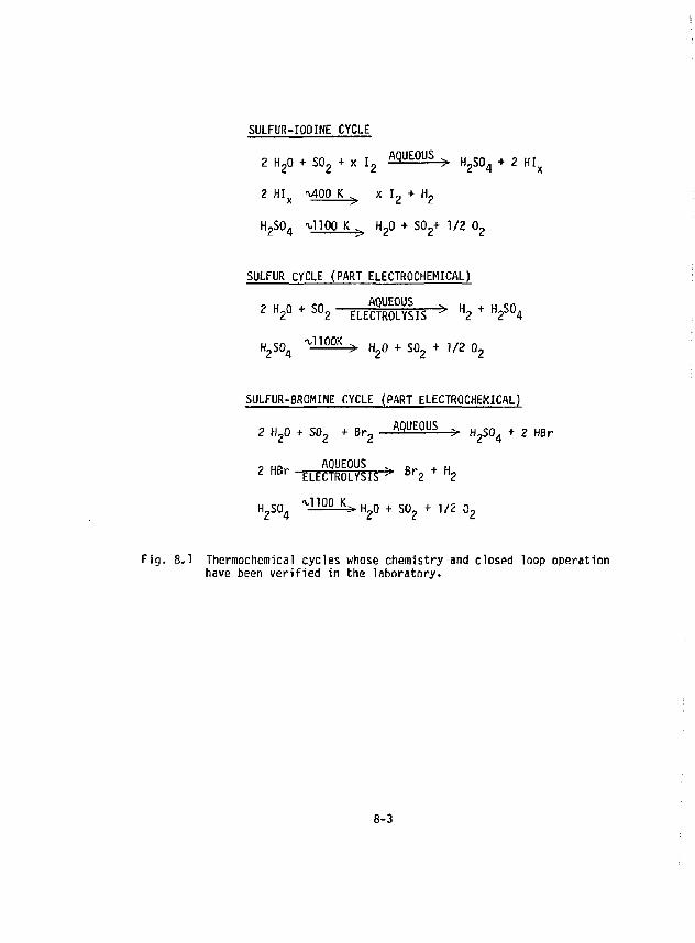
SULFUR-IODINE CYCLE

2 H 20 + S0 2 + x I 2 A Q U E 0 U S > H 2 S 0 4 + 2 HI

2 HI X VtOO K x I 2 + H 2

H 2S0 4 illOO K H 20 + S0 2+ 1/2 0 2

SULFUR CYCLE (PART ELECTROCHEMICAL)

2 H2° + S 02 E L E S Y S I S > H2 + H 2 S 0 4 H 2S0 4 ' v 1 1 0 0 K > H 20 +• S0 2 + 1/2 0 2

SULFUR-BROMINE CYCLE (PART ELECTROCHEMICAL)

2 H 20 * S0 2 + Br 2 AQUEOUS > H ^ + 2 H B r

? HRr- AQUEOUS - „„ . „ 2 H B r ELECTROLYSIS > S r 2 H 2

H 2S0 4 ^ H 0 0 K-> H 20 + S0 2 + 1/2 0 2

Fig. 8,1 Thermochemical cycles whose chemistry and closed loop operation have been verified in the laboratory.

8-3

cooldown, serious materials problems, and the need for considerable recycle because of low decomposition yields.

If the decomposition of water is carried out in two or more chemical reaction steps, a number of advantages result. For example, the production of H_ and 0, can be separated into different reaction steps, thus avoiding the back reaction problem. Also* by picking a proper combination of reactions, the maximum reaction temperature can be lowered with resultant benefits in reaction yields and availability of suitable materials. In actual practice, it is found that two-step cycles have shown only minimal lowering of the temperature compared to the single-step decomposition of water, unless one of the steps involves an electrochemical assist (e.g., see the Sulfur Cycle in Fig. 8.1). A cycle that includes an electrochemical step is called a "hybrid" cycle. With three or more steps, cycles based only on thermal input for the chemical reactions become possible at reasonable temperatures {e.g., see the Sulfur-Iodine Cycle in Fig. 8.1), and many will work efficiently at maximum temperatures of about 1200 K.

In order to illustrate some of the important considerations in developing and evaluating thermochemical cycles, we can use a generalized two-step cycle represented as follows:

T R + H20(ji) -i-> R0 + H 2(g), &G° < 0, AH° = AH-, (2)

RO — 5 - > R + V 2 0 2(g), t&° < 0, AH° = AH D (3)

In reaction (1), a reducing agent R is used to reduce water to produce H, at temperature T,, forming the oxide RO in the process. Reactions such as this are usually carried out near room temperature or at slightly elevated temperatures. In order to achieve a near zero or negative AG" to make the reaction go, the enthalpy change is usually governing and AH, is negative (an exothermic reaction). Heat produced by reaction (1) is usually of limited value for reuse in the cycle because of the low temperatures involved. Reaction (Z) is carried out at a high temperature, and is the decomposition step that regenerates the reducing agent R and 0«. Reaction

8-4

(2) is highly endothermic (AH Q is positive) and requires a large change in entropy (AS°) to produce a near zero or negative AG". This can be readily seen from the well-known second law expression AG" = AH° - TAS° where the TAS° term becomes increasingly important as the temperature is raised. Hence, one of the requirements in selecting RO is that it have as large a iS° of decom­position as possible, to minimize the maximum temperature required in the thermochemical cycle. As an example, the gaseous molecule SCU (R = S0~) meets the requirement for reaction (2), but S0 2 falls short of the require­ment for reducing water to produce Hg in reaction (1). The fix for this problem is to use an assist for reaction (1) by either (a) forming a hydro­gen impound of intermediate stability, such as HI or HBr, which can be subsequently decomposed to obtain the desired H^ product, or (b) using an electrolysis assist at a voltage substantially less than for direct water electrolysis (e.g., the Sulfur Cycle in Fig. 8.1). In the case of HBr decomposition, an electrolysis assist is also required {see Sulfur-Bromine Cycle in Fig. 8.1), since the yield is low for thermal decomposition of HBr.

Two types of cycle efficiencies are used in evaluating thermochemicf.l cycles. The work efficiency, i.e., the efficiency of converting heat irto work, E(w), is given by

The thermal efficiency, or the efficiency of heat utilization, E(H), is given by

E < H > = i l n § 1 '•« ^ ' <*) In expression (4), the number 237.2 (in kJ/mol) represents the maximum

work (flS°) available from the hydrogen produced, (see expression (1), while £AH D represents the total external heat requirements for the cycle, i.e., the heat provided by the non-fossil fuel heat source. For electricity required in the cycle, the Z/SHD term includes the equivalent heat required to produce the electricity; or as in the case of the Tandem Mirror Raac'or

8-5

as an energy source, some of the energy is available as electrical energy from the Direct Converter, and we add this directly to the £AH n term assuming it to be equivalent to thermal energy at 100% conversion. We see that E(w) is limited by a Carnot expression for the maximum efficiency. The thermal efficiency, E(H), compares the combustion energy of the hydrogen produced to form liquid water at room temperature as the final product, with IAH Q. The thermal efficiency could conceivably exceed the Carnot efficiency up to a maximum value given by the ratio of 285.8/237.2 = 1.21.

8.1.3 Some Important Criteria

A listing of the major reaction steps (such as in Fig. 8.1) gives only an indication of the complexity of a thermochemical cycle system. Choosing the best cycle and optimizing it in terms of efficiency and economics are challenging research goals. The criteria that must be considered include:

o Favorable thermodynamics.

o Fast reactions.

o High reaction yields.

o Simple separations.

o Process design factors (such as efficient use of heat, avoidance of scarce or hazardous reagents, and simplicity of construction).

Favorable thermodynamics implies both a negative and a very small free energy change (ijG0) for each reaction step. If the free energy change were positive, the equilibrium constant of the reaction would be unfavorable, and much energy would be wasted in separating or concentrating the reaction products. If the free energy change were too negative, on the other hand, one or more of the reaction products would be too stable and hard to

8-6

regenerate into the original reactants.

Fast reactions are desirable, e? ially for reactions involving gaseous reactants, because they enable us to use smaller and less expensive reaction vessels. The requirement that the free energy change be nearly zero makes it difficult to achieve fast reactions, however, because it allows very little driving force for the reactions. Reactions need to be selected in which the energy barriers are low enough to permit a very small free energy change to drive them rapidly. In many instances, the reaction rates can be enhanced by the use of catalysts.

High reaction yields are important to minimize recycling of unreacted reagents or diversion of material into undesirable by-products.

By u^ing simple separations, we can avoid another area in which hidden costs can be substantial. Operations such as boiling, compression, and filtering can involve expensive process equipment and energy losses, and they need to be minimized.

Mnally, careful process design can do much to provide the optimim tradeoff between the efficient use of heat energy and the ecnnomies of construction and operation. Process design contributions include new and innovative process equipment, plant layout, and siting.

8-7

8.2 GEXE8M. ATOMIC CYCIS

C.2.1 Selecting a Cycle

We have selected the GA Sulfur-Iodine Cycle for our current TMR/Thermo-chemical Cycle coupling studies because it is the closest of the most ad'/ancect cycles to a pure thermal cycle. This permits the economies of sca.ie to apply for chemical process units in a large chemical plant of the type conside*»ed here. Scale-up does not permit a similar reduction in costs for-electrolysis units which are modular in construction. The Sulfur-Iodine Cycle also involves the handling of only liquids and gases, which is advan^ tageous from a chemical engineering standpoint.

8.2.2 Chemical Description of GA Cycle

The current Sulfur-Iodine Cycle can be described chemically as follows:

2 H 20 + S0 2 + x I 2 -* H 2S0 4 + 2 HI x (390 K) (1) 2 HI X + H 2 + x I 2 (420 K) (2) H 2 S 0 4 + H 20 + S0 2 + 1/2 0 2 M 0 5 0 K-1250 K) (3)

A H reactions in this system have been verified in the laboratory and total recycle has been illustrated in a small closed-loop cycle experi­ment.* Major parts of the process are associated with separation and purification of the reaction products. A critical aspect for the successful operation of the process is the separation of the aqueous reaction products in reaction (1) above. Workers at the General Atomic Company have solved this problem by using an excess of I 2 in reaction (1), which leads to separation of the products into a lower density phase, containing HgSO. and H 20, and a higher density phase, containing HI, I 2 and K 20. Reaction (2) shows the catalytic decomposition of HI, which is carried out under pressure (^0 atm) with HI and I- in liquid forms, in order to enhance the decomposition yield. Laboratory decompositions are around 30* per pass and,

8-8

therefore, use a recycle step. Unreacted HI is condensed out of the H~ product and distilled away from the I~ product. Pure H, is obtained by scrubbing out the remaining I~ with H^O.

The equilibrium for reaction {3) lies to the right at temperatures above 1000 K, but up to temperatures of T-1150 K, catalysts are needed to attain sufficiently rapid decomposition rates. Catalysts are available for this process, but careful consideration needs to be given to cost versus effec­tiveness. The SO, Decomposition Reactor is a challenging unit to design, owing to the high temperatures and corrosive products involved. All of the HgSO, based cycles currently under study need such an SO-, decomposer. Each of the three laboratories involved has approached this problem from a differ­ent standpoint. The Joule-Boosted Decomposer introduced by LLNL in this year's study provides a breakthrough in this difficult area by overcoming the materials and catalyst problems, and giving increased decomposition yields.

Figure 8.2 is a simplified schematic flow diagram of the GA Sulfur-Iodine Cycle conceptually showing product flows and recycle streams.

A complete description of the GA Cycle is given later, in Section 9 of this report. For purposes of flowsheeting and process design, the GA Cycle has been divided into the following process sections.

o Section I, H-SO.-HI Production and Separation. o Section II, HpSO^ Concentration and S0 3 Decomposition. o Section III, HI Separation and Purification. o Section IV, HI Decomposition and H ? Purification. o Section V, Energy Distribution and the TMR-Chemical Plant

Interface.

8-9

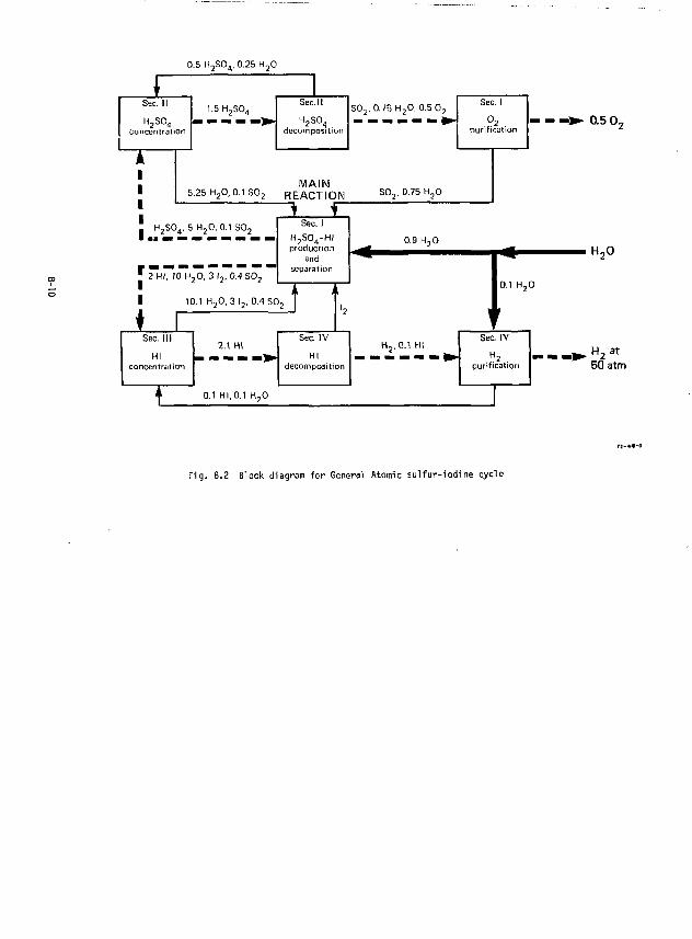
0.5 H 2S0 4, 0.25 H 30

" SEC. 11

H 2SO„ concentration

1 .5H 2 S0 4

Sec. 11

H 2 S 0 4

decomposition

S 0 2 , 0.75 H 2 0 , 0.5 0 2

Sec. 1

°2 purification

— — - > . 0.5 0.

A i i i

5.25 H 2 0 , 0.1 S 0 3 R MAIN

EACTIO 1

N S 0 2 , 0.75 H 2 0

A i i i >

MAIN EACTIO 1 f

i J 2 S 0 4 , 5 H 2 0 , 0.1 3 0 2

Sec. I

production and

separation

0.9 H 2 0 i Sec. I

production and

separation

0.9 H 2 0

• 2 HI, 10 H,0. 3 l 2 , 0.4 SO,

Sec. I

production and

separation

0.1 H 2 1 1 1

10.1 H 2 0 , 3 l 2 , 0.4SC n i

2 i

'2

0.1 H 2 1 1 1

i

'2

0.1 H 2

Sec. I l l

HI concentration

2.1 HI Sec. IV

HI decomposition

H j . 0 . 1 HI Sec. IV

H 2

purification - - _ • H 2 at

50atr

t 0.1 HI,0.1 H 2 0

Fig. 8.2 Block diagram for General Atomic sulfur-iodine cycle

8.3 THERMODYNAMIC DATA BASE FOR SECTION II

The thermal efficiency for conversion of water to hydrogen is very sen­sitive to heat-matching in the thermochemical process plant. This conversion efficiency directly impacts the capital cost of the total plant, including the TMR energy source. For examp'e, for a given hydrogen production rate, an increase of 10S! in cycle efficiency would lead to an approximate 10% reduction in size and cost for both the TMR and the chemical plant.

A large proportion of the energy supplied by the TMR is required for operation of Section II. Primary reactor heat put into Section II is generally recovered and reused several times before discharge as waste heat. Because of the large magnitude of heat handled in this Section, proper heat-matching and reuse of heat are very critical to achieving a high efficiency process. Furthermore, the accuracy of the thermodynamic data base used here is important if we are to achieve a realistic optimum or near optimum in efficiency of heat utilization in Section II.

Only a portion of the thermodynamic data that are needed to do heat-matching and mass and energy balances for Section II is currently available in the literature. However, we are able to fill in some portions of the missing data by deriving approximate thermodynamic data based on recent unpublished measurements by Lennartz, ' who gives pressure-composition-temperature (P,x,T) data for the M 20-H 2S0 4 system. In addition, for our current purposes, we have made some additional rough estimates as needed in order to obtain a complete thermodynamic data base for use in Section II. This data base will be described and summarized in the following sub-sections.

8.3.1 Sequence of Process Steps

Before developing the thermodynamic data, we briefly describe below and in Fig. 8.3 an illustration of the process steps for which the thermo­dynamic data will be used. The illustration given here is for the Joule-boosted decomposer approach.

8-11

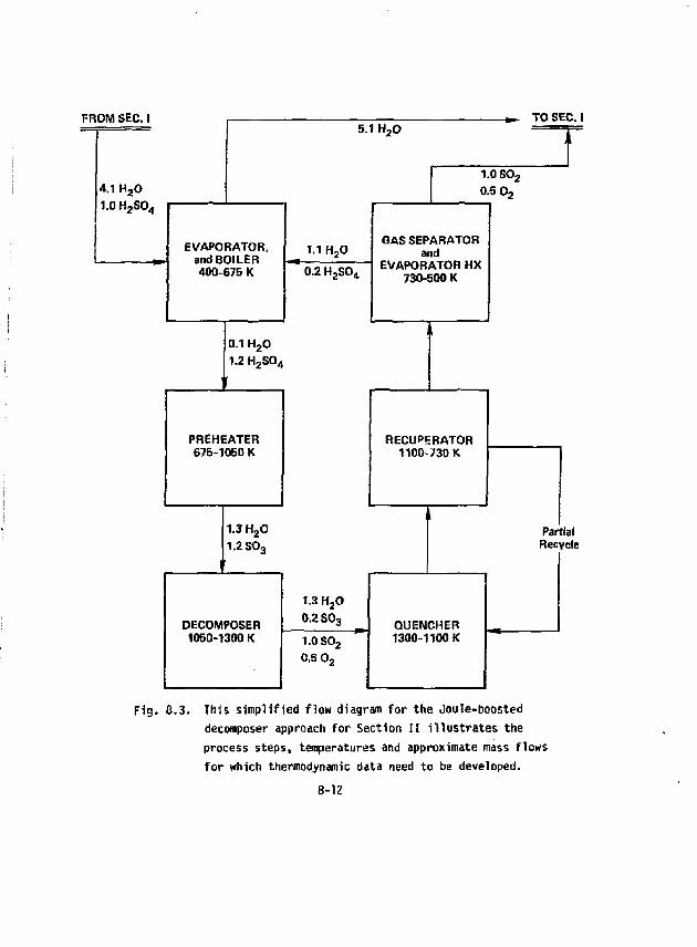
FROM SEC. 1 TO SEC I FROM SEC. 1

4.1 H 2 0 1.0 H 2 S0 4

t 4.1 H 2 0 1.0 H 2 S0 4

1.0 S0 2

0.5 0 2 4.1 H 2 0 1.0 H 2 S0 4

EVAPORATOR, and BOILER 400-675 K

1.1 H 2 0 GASSEPARATOR

and EVAPORATOR HX

730-500 K

EVAPORATOR, and BOILER 400-675 K 0.2 H 2 S0 4

GASSEPARATOR and

EVAPORATOR HX 730-500 K

1

0.1 H 2 0 1.2 H 2 S0 4

I

1 1

PREHEATER 675-1050 K

RECUPERATOR 1100-730 K

PREHEATER 675-1050 K

RECUPERATOR 1100-730 K

Par Rec

'

1.3 H 2 0 1.2 S0 3

Par Rec

•If

DECOMPOSER

1.3 H 2 0 0.2 S0 3 QUENCHER

Par Rec

1050-1 300 K i.o so 2

0.5 0 2

1300-1 100 K

Fig. 6.3. This simplified flow diagram for the Joule-boosted decomposer approach for Section II illustrates the process steps, temperatures and approximate mass flows for which thermodynamic data need to be developed.

8-12

Concentration of H ?SO,. The feed material for this process step consists of two streams: (1) the 57 w W (20 mole %) sulfuric acid product from Section I at -vftOO K wnich supplies about 80% of the feed, and (2) a 50 wt% (15 mole %) sulfuric acid from tne decomposer product stream at about bOO-600 K wnich makes up the balance of the feed. These acid streams are concentrated in sulfuric acid by selectively vaporizing off water in a staged evaporator to produce the 98 wt% (90 mole %) H 2S0 4 azeotrope at ^675 K. Pure water recovered from the evaporation is returned to Section I.

Boiling of Azeotrope. The 98 wt% hLSO^ azeotrope is boiled isothermally at about 5 atm and 670 K to obtain the gaseous feed for the decomposer. Gaseous species produced by the boiler are H.SO., S0 3 and H-O.

Preheating of Gas. The gas from the boiler is preheated from i670 K to about 1000-1100 K to prepare it as feed to tne decomposer. Molecular H 2 S 0 4 decomposes endothermically to S0 3 + H 20 during this preheat.

Decomposition of SQ... The gaseous feed from the preheater now contains about 50 mole % each of S0 3 and H 20. About 90?S of the S0 3 is decomposed at 6 atm and 1300 K to form SO^ and 0 2 as products.

Cooluown of Decomposition Products. The gaseous products from the aecomposer are quenched to 1.1100 K to prevent back reaction of S0~ + 0 ?. Quencning is accomplished by recycling some of the cooled decomposition product gases into the decomposer product stream. The product strecsn is tnen passed through a tube and shell recuperator to preheat the gas feed entering tne decomposer. A portion of tne cooled recuperator output gas (at V O 0 K) is used as quench gas (see above) and the balance is used to supply heat to the evaporator through a heat exchanger, (jndecomposed SO. remaining in the product gas combines with H~0 and condenses out as aqueous H 2S0 4 at about 500-600 K. This aqueous HpS0 4 is added to the evaporator stream for recycle, and gaseous SO, and Op are separated and sent to Section I.

8-13

8.3.2 Thermodynamic Data Requirements

The thermodynamic data requirements for each of the process steps described above will now be discussed in a general way. Details of the data derivation and methods for use of tlie tnermodynamic data are covered in a later subsection.

Thermodynamic Pata for Concentration of HTSO.

As the sulfuric acid solutions are concentrated in a staged evaporator, we need to have information on several thermodynami- parameters for each stage, i.e., (1) we need to know the uptake of sensible heat as the solution is heated, (2) the vapor pressures of gaseous products and the resultant change in liquid phase composition, (3) the vaporization enthalpies to the gas phase, (4) the sensilbe heat, the condensation temperature and the condensation enthalpy of the gas phase product, and (5) the sensible heat available in the condensate as it cools.

The chemical processes occurring in a single evaporation stage and the approximate enthalpy cl.anges associated with the processes are illustrated in che following simplified example.

lH 2S0 4 + 4 H 20) •* (H2S04 + 4 H 20); A H l a = 35.7 kJ/mol (lla) 400K, aq 600K, aq

(H 2S0 4 + 4 H 20) + (H 2S0 4 + 3 HgO) + H20{8,); W]b = 8.1 U/mol (l'b)

(lie)

(12)

(13)

bOOK, aq 600K, aq 600K, 1 atm

H20(JL) 600K, 1 atm

-*• H20(g) ; fiH1c = -27.1 kJ/mol 600K, 40 atm

H 2o(g) 600K, 40 atm

•*• H 20(g) ; AH 2 = -4.2 kJ/mol 525K, 40 atm

H 2o(g) 52 5K, 40 atm

+ H20(i,) ; W3 = -29.5 kJ/mol 525K, 40 atm

8-14

H20(x.) + H20(Ji.) ; AH 4 = -8.9 kJ/mol (14} 525K, 40 atm 430K, 5.6 atm The first reaction above, corresponding to the uptake of enthalpy and

boiling off of part of the water, is broken down into three parts for the Convenience of thermodynamic calculations. Thus, (11a) represents the increase in sensible heat of the initial (H„S0 4 + 4 H ?0) solution, (lib) represents the exsolution of water into a hypothetical 1 atm reference state, a.nd (lie) the boiling of the 1 atm reference state of water to the equilibrium partial pressure of steam above the final (H„S0. + 3 H ?0) solution. The equilibrium steam pressure is estimated by extrapolating the data of Lennartz to higher pressures.

Reactions (12), (13), and (14) represent the enthalpy available for reuse in the evaporated steam. This enthalpy is available as sensible heat in the steam, the condensation energy of the steam, and sensible heat in the condensed water down to 430 K. Thus, with a total enthalpy input of 70.9 kJ/mol (35.7 + 8.1 + 27.1), 42.6 kJ/mol (4.2 + 29.5 + 8.9) or 60% is available for reuse above 430 K, with most of it actually available above ^biiO K. The balance of the enthalpy -emains primarily as sensible h^at in the concentrated sulfuric acid.

In subsequent evaporation stages as the H-SO* is heated hotter and gets more concentrated, the thermodynamics get complicated, as first HnSO-(g) and then SOqfg) contribute in increasing amounts to the gas-phase composition. Upon reaching the azeotrope composition, the gas phase wfN consist of roughly 40% H-SO.fg) and 30% each of S0-(g) and H„0{g). Also, the entr ,py for exsolution of H20(fc), reaction (lib) above, will increase by ner iy an order of magnitude. Thus, for the more concentrated H ?S0- solutions the condensate from the gas phase will contain a substantial amount of H ?S0., and several additional evaporation stages are needel to obtain a separation of relatively pure water. Consequently, *>oth the complexity of the H ?S0. concentration process and the energy requirements increase as the azeotrope is approached; and it becomes especially important in this region to have accurate thermodynamic data and to do careful heat-matching.

8-15

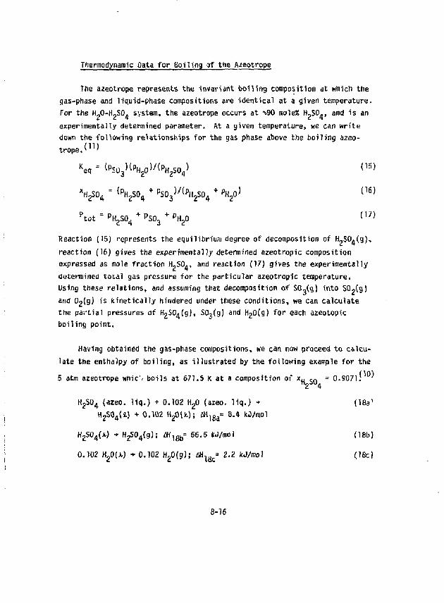
Thermodynamic Data for toiling of the Aieotrope

The azeotrope represents the invariant boiling composition at which the gas-phase and liquid-phase compositions are identical at a given temperature. For the HgO-hLSO, system, the azeotrope occurs at -\90 mole* H.SCL, and is an experimentally determined parameter. At a given temperature) we can write down the following relationships for the gas phase above the boiling azeo­trope.' '

Keq = ^S0K\QV%S0J < 1 5>

xHgS0 4 = { p H z S 0 4

+ P S 0 3) / ( P H 2 S 0 4

+ ^ ^

Ptot = PH 2S0 4 + PSD 3

+ \0 < 1 7 )

Reaction (15) represents the equilibrium degree of decomposition of HUSO^g), reaction (16) gives the experimentally determined azeotropic composition expressed as mole fraction H,S0., and reaction (17) gives the experimentally determined total gas pressure for the particular azeotropic temperature. Using these relations, and assuming that decomposition of SG,(g) into S0 2(g) and 0 2(g) is fcinetically hindered under these conditions, we can calculate the partial pressures of H 2$0 4(g), SOjfg) and H 20(g) for each azeotopic boiling point.

Having obtained the gas-phase compositions! we can now proceed to calcu­late the enthalpy of boiling, as illustrated by the foUowing example for the 5 atm azeotrope whic'i boils at 671.5 K at a composition of x„ s „ = 0.9071: '

H 2S0 4 {azeo. liq.) + 0.102 H 20 (azeo. liq.) + (18a1

H ZS0 4(1J + 0.102 H 2 0 U ) ; *H}8 aa 8- 4 W m o l

H 2S0 4(A) - H ^ O ^ g ) ; * 1 8 b = 56.5 KJ/moI (18b)

0.102 H20(J(.) * 0.102 H20(g); tM^ 2.2 W/mol (18c)

8-16

H 2S0 4(g) + 0.620 H 2S0 4{g) (18d) + 0.360 SO (g) + Q.38Q H 20(g); tii^ = 35.9 kJ/raol

Here again the reactions are broken oown into intermediate steps for thermo­dynamic convenience, with H-SO^Ji) and HgQU) representing 1 atm hypothetical reference states. The sum of the enthalpies for (18a) through (18d) gives 103.0 fcJ/mole, which represents tne boiling enthalpy per mole of H„SQ. for the 5 atm azeotrope.

Thermodynamic Data for Preheating the Gas

Molecular H 2S0 4(g) gradually decomposes into S0 3(g} and H zO(g) as tne azeotropic gas mixture is preheated from the boiling point up to the point where it is introduced into the decomposer. It is assumed that the H ^ O ^ g ) decomposition equilibrium is rapid, and that the decomposition of S0j{g) into S0 2(g) and 0 2(g) does not occur because it is kinetically hindered. Thermo­dynamic data that are required are the equilibrium constant for H 2S0 4(g) decomposition; enthalpies for the sensible heats of gaseous H2S0,,, S0 3, and HyO; and the decomposition enthalpy of gaseous H 2S0 4. An illustration of the calculations involved is given in an earlier report. '

Thermodynamic Data for Decomposition of SO3

Decomposition of SQ,(g) is assumed to reach equilibrium at the exit temperature and pressure of the decomposer. Thermodynamic data required are tne equilibrium constant and enthalpy for decomposition, and enthalpies for the sensible neat changes in the gaseous species between inlet and outlet of the decomposer.

Thermodynamic Data for Decomposition Products

The thermodynamic data required for cooldown of the decomposition products involves enthalpies for sensible heats, recombination enthalpies, condensation enthalpies, and various equilibrium constants. Data for these processes are similar to that during htatup.

8-17

8.3.3 Summary of Thermodynamic Data

A summary is given here of the current status of the thermodynamic data base. Major progress has been made during the past year in bringing this data base up to date and putting it into a form where it can be used to obtain reasonably accurate energy balances for Section II. Some work still remains to complete the data evaluations and summaries. The next step would be to convert the data base into a form suitable for computer use in doing process optimization.

Table 8.1 provides a concise summary of the thermodynamic data require­ments, the current data sources, and a listing of the tables and figures in this section that summarize the current data. In t> e discussions that follow, we describe the bases for the data.

Equilibrium Constant Data

Of the items designated in Table 8.1 under equilibrium constant data, the partial pressures of gaseous species above aqueous HpSO* <:nd the azeo-trope parameters are the most difficult data to obtain. The balance of the

(12 11} items are readily cbtained from standard tabulations.1 ' '

Some years ago, Gmitro and Vermeulen*- *' did an excellent theoretical job of calculating the equilibrium vapor compositions above H-O-H.SO. mix­tures up to 673 K. The difficulty with their work was that they were limited Lo the room temperature experimental data of Giauque and coworkers'' ' for Input aata. As a consequence, their high temperature data do not agree with the recent experimental total pressure values and azeotrope compositions of Lennartz.' 1 0)

Lennartz's total pressure data is summarized in tabular form in Table 8.2, and in graphical form in Fig. 8.4. Pressures and temperatures in Fig. 8.4 nave been extrapolated beyond the experimental range for convenience in doing pressure-staging calculations for the evaporator process step. An example of Gmitro and Vermeulen's data is given in Fig. 8.5. Note that the propor-

8-18

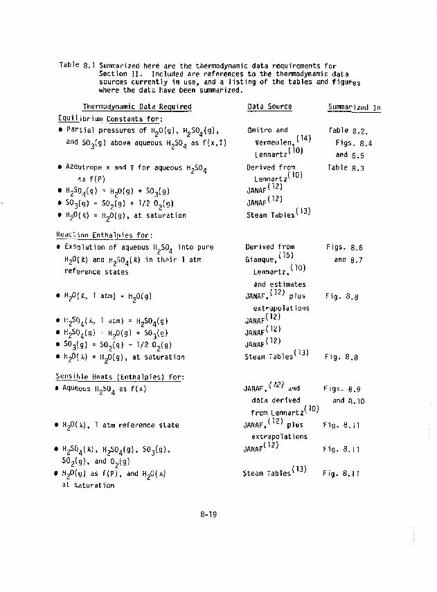
Table 8.1 Summarized here are the thermodynamic data requirements for Section II. Included are references to the thermodynamic data sources currently in use, and a listing of the tables and figures where the data have been summarized.

Lennartz

Thermodynamic Data Required Data Source Equilibrium Constants for: • Partial pressures of HpO{g), HpSO.fg), Gmitro and and 50 3(g) above aqueous H^SO* as f(x,T) Vermeulen,

• Azeotrope x and T for aqueous hUSO* « f(P)

• H 2SQ 4(g) = H20(g) + S0 3( 9) • S0 3(g) = S0 2(g) + 1/2 0 2(g) • H20(H) = H 20(g), at saturation Steam Tables

Reaction Enthalpies for: • Exsolution of aqueous H ?S0. into pure

H 20(£) and H2S04(A.) in ths>ir 1 atrc reference states

(14) 10)

Derived from Lennartz^ '

12) JANAF JANAF :i2)

(13)

Derived from Giauque/ 3'

Lennartz, ;io)

and estimates 12) JANAF,

extrapolations 12)

• H20(i, 1 atm) = H20(g)

• H 2S0 4(H, 1 atm) = H 2S0 4(g) • H2S()4(g) = H 20(g) + S0 3(g) • S0 3(g) = S0 2(g) + 1/2 0 2(g) • H20(i,) = H 20(g), at saturation Steam Tables

Sensible Heats (Enthalpies) for: • Aqueous H 2S0 4 as f(x) JANAF,

plus

JANAF JANAF JANAF

(12) 12)

<W

13)

and data derived from Lennartz

:i2)

Summarized In

Table 8.2, Figs. 8.4 and a.5

Table 8.3

Figs. 8.6 and 8.7

Fig. 8.a

(10)

Fig. 8.8

Figs. 8.9 and e.10

JANAFv

• H 20(JL), 1 atm reference state

• H2SQ4(jt), H 2S0 4(g), S0 3(g), S0 2(g), and 0 ?(g)

• H 20(g) as f(P), and H20{Jt) Steam Tables at Saturation

JANAF,v ""' plus Fig. 8,11 extrapolations

: ( 1 2 ) Fig. 8,11

13) Fig. 8,1

8-19

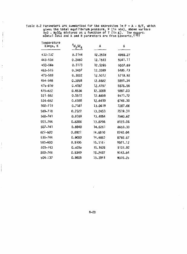
Table 8.2 Parameters are summarized for the expression In P = fc - B/T, which gives the total equilibrium pressure, P ( in atm), above various H2O - H3SO4 mixtures as a function of 7 ( in K). The experi­mental data and A and B parameters are from Lennartz.('0}

Range, K xH 2S0 4

0.2144

A B

433-532

xH 2S0 4

0.2144 12.2538 4968.27 443-538 0.2460 12.1593 5041.11 453-56b 0.3173 12.5265 5507.69 463-575 0.3407 12.3389 5485.73 473-588 0.3832 12.5012 5718.92 464-598 0.3998 12.6682 5891.34 476-610 0.4187 12.4767 5875.56 479-622 0.4536 12.3088 5887.03 521-652 0.5512 12.6858 6471.72 534-682 0.6388 12.6410 6746.30 502-719 0.7181 13.0419 7287.66 589-718 0.7522 13.2453 7519.31 568-741 0.8189 13.4854 7840.62 503.744 0.8386 13.8296 8123.06 507-741 0.8840 14.5261 8659.33 621-693 0.8921 14.6010 8740.04 535-744 0.9050 14.6863 8792.67 583-603 0.9195 15.1161 9071.12 503-743 0.929b 15.1626 9101.92 503-744 0.9349 15.2487 9143.64 504-737 0.9B06 15.3841 9076.25

8-2D

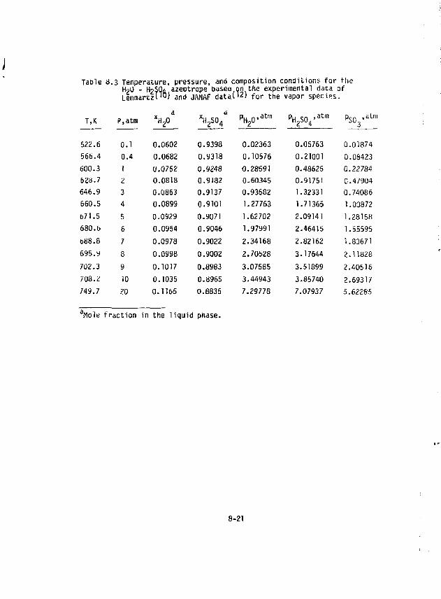
TaDle 8.3 Temperature, pressure, and composition conditions for the HpU - HpSOji azeotrope baseti qn the experimental data of LennartzH") and JANAF datal 1 2) for the vapor species.

T,K P,atm *H20 V°4 P H 2 0 ' a t m P H 2 S 0 4 ' a t m Ps^.atm

522.6 0.1 0.0602 0.9393 0.02363 0.05763 0.01874 566.4 0.4 0.0682 0.9318 0.10576 0.21001 0.08423 600.3 J 0.0752 0.9248 0.28591 0.48625 0.22784 628.7 2 0.0818 0.9182 0.60345 0.91751 0.47904 646.9 3 0.0863 0.9137 0.93582 1.32331 0.74086 660.5 4 0.0899 0.9101 1.27763 1.71365 1.00872 671.5 5 0.0929 0.9071 1.62702 2.09141 1.28158 680. b 6 0.0954 0.9046 1.97991 2.46415 1.55595 688.8 7 0.0978 0.9022 2.34168 2.82162 1.83671 695. y 8 0.0998 0.9002 2.70528 3.17644 2.11828 702.3 9 0.1017 0.8983 3.07585 3.51899 2.40516 708.2 10 0.1035 0.8965 3.44943 3.85740 2.69317 749.7 20 0.1165 0.8835 7.29778 7.07937 5.62285

Mole fraction in the liquid phase.

8-21

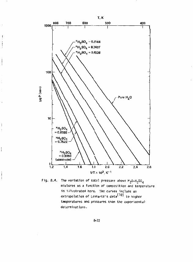
T, K

1000 800 700

100

600

- x H z S 0 4 = 02144 -*H 2S0 4 =0.3407

•- 0.4536

500 400

Pure H 20

1.8 2.0 2.2 1/TX 103.K-1

2.6

Fig. 8.4. The variation of total pressure above H,0-H?S04

mixtures as a function of composition and temperature is illustrated here. The curves include an extrapolation of Leunartz's data' °' to higher temperatures and pressures than the experimental determinations.

8-22

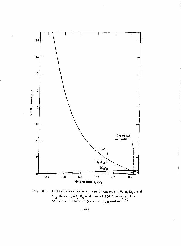
16

14 ^

12

S 10

Azeotrope compasition-

H,0-

H 2 S0 4

SO.

^ 0.4 0.5 0.6 0.7 0.8 0.9

Mole fraction H 2 S0 4

F ig . 8.5. Par t ia l pressures are given of gaseous H^O, H-S0„, and SO, above Ho0-H,S0« mixtures at 600 K based on tine

(U) calculated values of Graitro and Venneulen. '

8-23

tion of H 2S0 4{g) in the vapor does not become important until ^85 wt* (50 mole*) H 2S0 4, and for S0 3(g) until -\85 wt% (80 mole %) HgSO^ is reached.

Enthalpy of Reaction Data

Most of the enthalpy of reaction data that is required here can be readily obtained from Standard compilations such as the JANAF Tables^ 1 2) anc Steam Tables' 3' {see Table 8.1). However, it is difficult to obtain Qata for the exsolution of aqueous ti^G^ into its pure components as indicated in reaction (18a), and an extrapolation needs to be made to higher temperatures to obtain data for vaporization of H-O(x) from its 1 atm reference state to HgO(g) (see reaction (18c)).

For exsolution of aqueous H,SOrt into its components at room temperature, we have available the excellent experimental data of Giauque et al.* ' These data are illustrated in terms of the solution reactions in Figs. 8.6 and 8.7 for the partial molal and integral enthalpies of solution at 298.15 K. (Entnalpies of exsolution are the negatives of these values.)

At higher temperatures, i.e., at ^600 K, we have derived approximate values for the enthalpies of solution from the P,x,T data of Lenn&rtz.' ' Thus, examining Lennartz's data in Table 8.2, we find that the product of the gas constant R times the parameter B is the total enthalpy of vaporization for all gaseous species at ^600 K above the various aqueous H SO. solutions. Furthermore, based on the calculations of Gmitro and Vermeulen^ ' (see Fig. 8.5), the vapor consists dominantly of H.O(g) up to about x = 0.6. Hence, by subtracting out the vaporization

c. HOOUA

enthalpy of H20(fc) in its 1 atm refere ice state from Lennartz's enthalpy of vaporization values, we obtain tne partial molal enthalpy of exsolution of HJ)(x<) at 600 K up to x H S n = 0.6. We can also obtain an additional value for the partial molal enthalpy of exsolution of H,0{£) at the azeo-trope composition by using the azeotropic relationships given by equations (15), (16), and (17) to obtain the partial pressure of H,0(g) as a function of temperature based on Lennartz's data. A ln(p„ „) versus 1/T plot

8-24

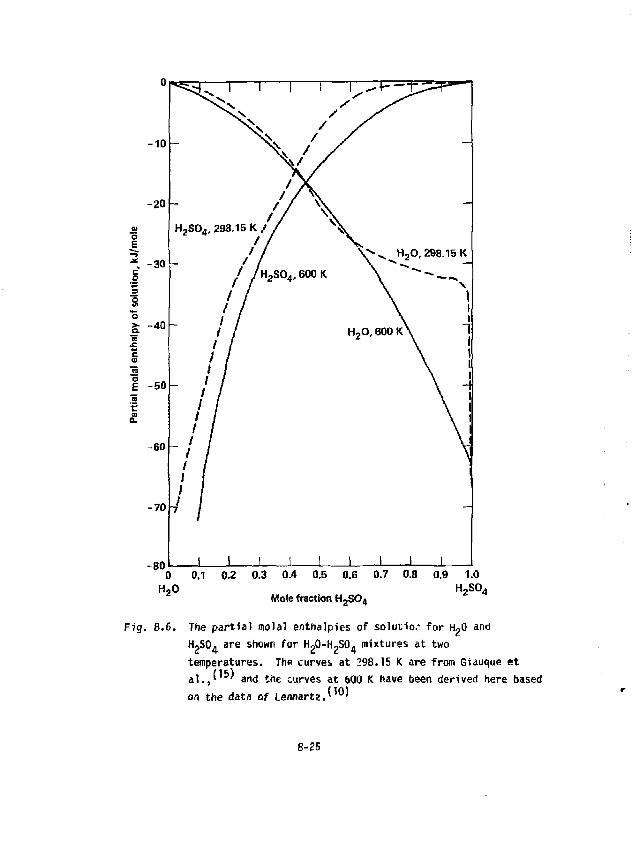
c a

o > • EL

I I

u

10 -

20

H 2 S0 4 , 298.15 K / / N >

/ /

/ / H 2 S 0 4 , 600 K

/ / / /

-

30

H 2 S0 4 , 298.15 K / / N >

/ /

/ / H 2 S 0 4 , 600 K

/ / / /

\ > . . HoO, 298.15 K \ «T —

\ \ 40 ' / / /

/ / / /

H 2 0,600 K \ 1

50 I 1 1 f ^

60

/ / / / / /

r ' / / / / / / /

N 70

art

4 j

i i i i i 1 1 1 0 0,1 0.2 0.3 0.4 0.5 0.6 0.7 0.8 0.9 1.0

H z S 0 4 H 20 Mole fraction H 2 S 0 4

Fig. 8.6. The partial molal enthalpies of solution for H ?0 and rUSO, are shown far HpO-H^SO, mixtures at two temperatures. The curves, at 298.15 K are from Giauque et al.,' ' and the curves at 600 K have been derived here based on the data of Lennartz/ °'

8-25

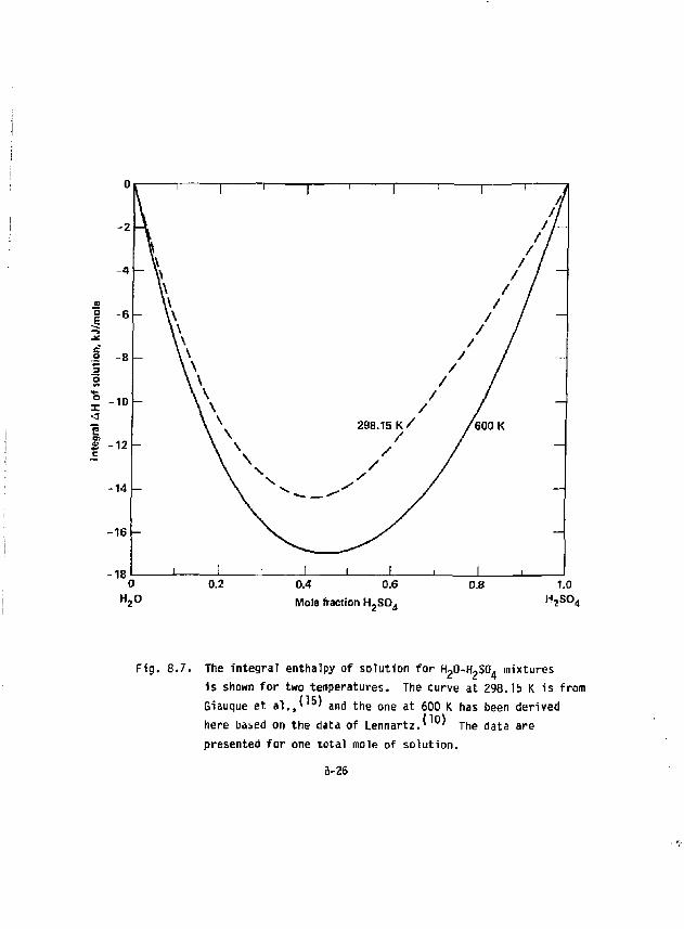
H20 Mole fraction H 2 S D 4

Fig. 8.7. The integral enthalpy of solution for ^O-HpSO. mixtures is shown for two temperatures. The curve at 298.15 K is from Giauque et al.,(' 5' and the one at 600 K has been derived here based on the data of Lennartz.* °' The data are presented for one total mole of solution.

a-26

then gives the enthalpy of vaporization of H?0(g) from the azeotropic com­position, and subtracting out the enthalpy of vaporization of the reference state H?0(>0 gi<fes the enthalpy of exsolution, as before. Tnese data, extending over the range of x u <-n = 0.2 to 0.9, allow us to construct the

"2 4 partial molal enthalpy of solution curve for H ?0 at T-600 K as shown in Fig. 8.6. The curve for HSC^ at 600 K is then derived from the H 20 curve oy using a Gibbs-Duhem integration procedure.

The integral enthalpies of solution (given in Fig. 8.7) are obtained by summing the partial molal enthalpies of solution as follows:

*I " \0 ^H 20 + X H 2 S 0 4 ^ H 2 S 0 4 < 1 9)

Thus, tne integral enthalpy of solution, ZsH., represents the solution enthalpy for one total mole of solution, and must be multiplied by the sum nf the moles of H ?0 + H ?S0. involved, when making calculations. It is more convenient for our purposes to use integral rather than the p&rtia] molal enthalpies of solution for calculations. Interpolations and extra­polations can be made as needed in Fig. 8.7 to oDtain data at intermediate and higher temperatures.

Values for the enthalpy of vaporization of water from the hypothetical 1 dtm reference State (see Fig. 8.8) were obtained as follows. Data up to bOO K were taken directly from the JANAF Tables, (^ while at higher tempera-turps un extrapolation was made down to 1 atm from higher pressure JANAF data. As is apparent in Fig. 8,8, there is a significant difference between the enthalpy of vaporization of water in its 1 atm reference state and at saturation.

Data on Sensible Heats (Enthalpies)

The area of greatest need for sensible heat (enthalpy increment) data is for aqueous MySO. as a function of composition (see Tabie 8.1). Data for the pure liquids and gases are either generally available in standard tabula­tions, or can be obtained by extrapolations.

8-27

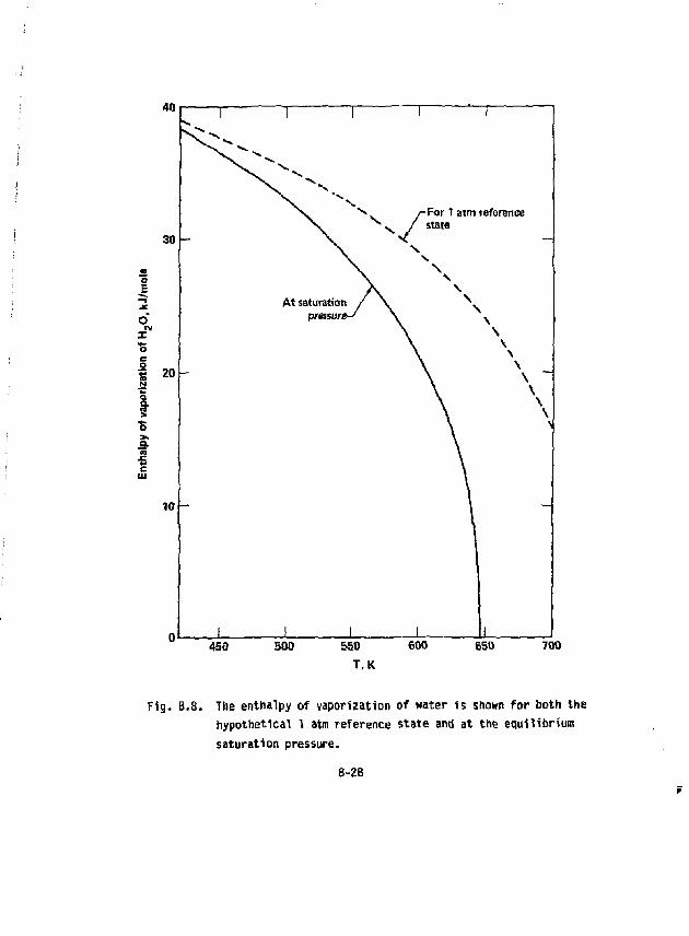
40

O tv

X

^ /-For 1 aim reference X

N / state

\

o s 20

8. S <•> o >> a

450 500 550 T.K

600 650 700

Fig. 8.8. The enthalpy of vaporization of water is shown for both the hypothetical 1 atm reference state and at the equilibrium saturation pressure.

8-28

There are two sources of data that we can draw on to estimate the enthalpy increments for aqueous HpSO- : (1) values for Hg^-Hgng derived from Lennartz's data,^ 1 0^ and (2) the JANAF Tables' 1 2) which summarize enthalpy increments for several compositions ranging from H ?S0«'H ?0 to H 2S0 4«6.5 H ?S0 4.

To illustrate the derivation of H f i n n-H ?<j 8 values from Lennartz's aata, consider the solution reaction:

0.6 H^OU) + 0.5 H2S04(Ji,) = 0.5 H 2S0 4-H^K.) (20)

Here pure liquids H ?0 and H„S0. in their 1 atm reference states are combined to produce a 50:50 mole ratio solution. ^ 6 0 0 _ i H 2 9 8 f o r t h e o v e r a 1 1 reaction is obtained from Fig, 8.7 and is found to be -16.87 - (-13.92) = -2-95 kj/mol. This can be equated to the difference in individual H g 0 0 - H 2 values between the product 0.5 H2S04'H20(Jt,) and the reaclants. Thus X - 0.5(25.648) -0.5(50.639) = -2.95, and X = 70.388 kJ/mo? for the H 6 0 0 - H 2 9 8 value of 0.5 H^Ojj'HpO. H 6Qy-H 2 9g values thus derived as a function of composition across the H ?0 - H-SCL diagram are summarized in Fig. 8.9.

A comparison can now be made of the Hcnn'^sqB values derived from Lennartz with the JANAF data (see Fig. 8.10). We find that agreement is good for the two compositions HpS0 4*H 20 and H 2S0 4«2 H-0, but that a major discrepency occurs in the more dilute H 2S0, concentrations. A comparision cannot be made at higher H 2 S 0 4 concentrations since JANAF data is not available. We believe that the values derived from Lennartz's data are the more reliable. Further work is needed to develop the data base over the full range of temperatures needed for the process studies.

Enthalpy increments for the other chemical substances involved in Section II are summarized in Fig. 8.11. Note the difference in enthalpy increments for saturated liquid H 20 and the 1 atm liquid H_0 reference state. Note also the differences in enthalpy increments for steam taken at different pressures.

8-29

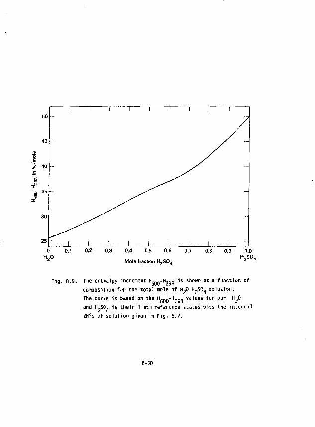
Mole fraction H , S 0 4

Fig. 8.9. The enthalpy increment Hg 0 0-H~g 8 is shown as a function of composition for one total mole of HgO-HgSO^ solution. The curve is based on the H^gg-H-™ values for pur H 20 and H 2S0. in their 1 atm reference states plus the integral 4H°s of solution given in Fig. 8.7.

8-30

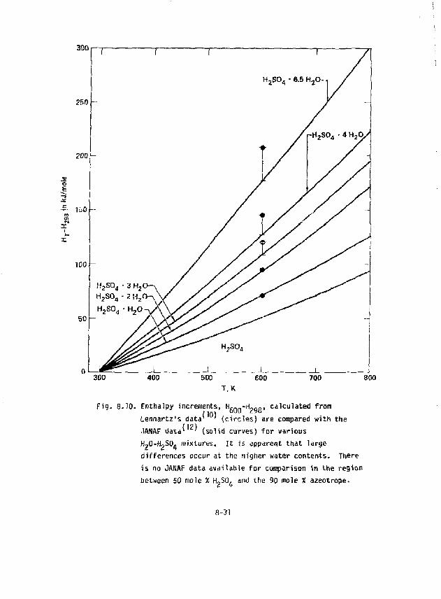
300

>-x

300 400 500 600 700 800 T.K

Fig. 8.10. Enthalpy increments, H , n n - H , Q 0 1 calculated from {101 Uennartz's data 1 ' (circles) are compared with the

.IftNAF data' 12) HgO-HoSO. mixtures

(solid curves) for various It is apparent that large

differences occur at the higher water contents. There is no JANAF data available for comparison in the region between 50 mole % H,S0. and the 90 mole 3! azeotrope.

fl-31

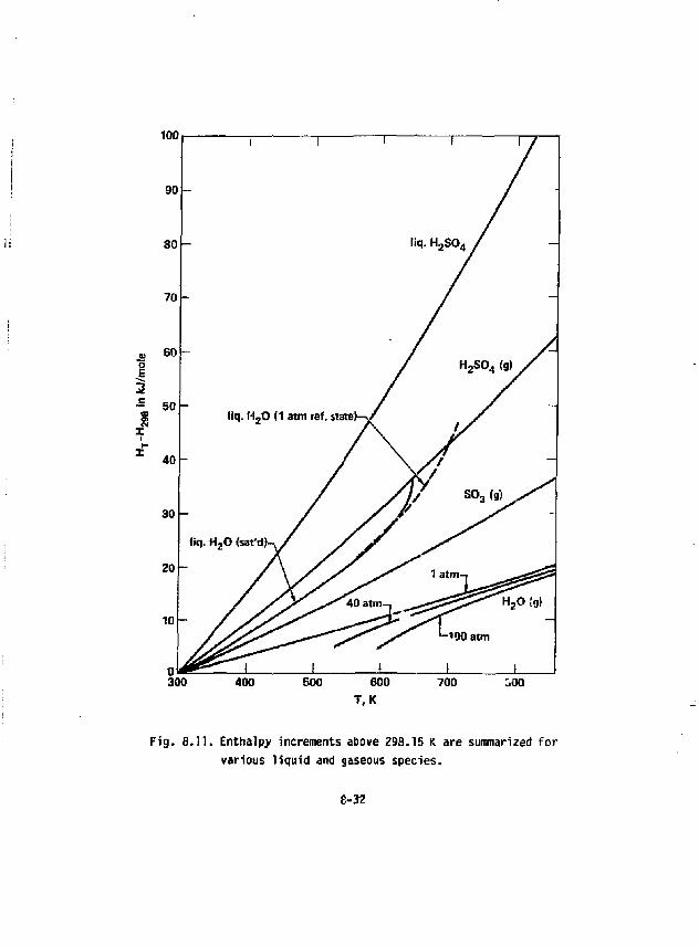
100

~ 50

X f

I

liq. M zO (1 atm ref. state;

Fig. 8.11. Enthalpy increments above 298.15 K are summarized for various liquid and gaseous species.

8-32

References for Section 8

K R. H. Werner, et al., "Synfuels From Fusion-Producing Hydrogen With the Tandem Mirror Reactor and Thermochemical Cycles," Lawrence Livermore National Laboratory, Report UCID-18909, Vol I. and II, , January 21, 1981.

2, G. £. Besenbruch, K. H. McCorkle, J. H. Norman, 0. R. O'Keefe, J. R. Schuster, and M. Yoshimoto, "Hydrogen Production by the GA Su1fur-Iodine Process. A Progress Report," in Hydrogen Energy Progress, Proceedings of the 3rd World Hydrogen Energy Conference, Tokyo, Japan. 23-26 June 1980, Vol.1, edited by T. N. Veziroglu, K. Fueki, arid r; Uhta, Pergamaon Press- Oxford, 1980, p. 243.

3< J. H. Norman, K. Mysels, R. Sharp, Cm! G. G. Williamson, "Studies 0 f the Sulfur-Iodine Thermochemical Water-Splitting Cycle," ibid., p, 257.

4. D. R. O'Keefe, and J. H. Norman, "The Liquid Hydrogen Iodide Decomposition Process Step for Water Splitting Applications," ibid., p. 277.

5» P. W. T. Lu and R. L. Ammon, "Development Status of Electrolysis Technology for the Sulfur Cycle Hydrogen Production Process," ibid., p. 439.

6. H. A. Irwin and R. I. Amman, "Status of Materials Evaluation for Sulfuric Acid Vaporization and Decomposition Applications," in Hydrogen Energy Progress, Proceedings of the 3rd World Hydrogen Energy Conference, Tokyo, Japan, 23-26 June 1980", Vol.4, edited by T. N. Veziroglu, K. Fueki, and T. Ohta, Pergamaon Press, Oxford, 1981, p. 1977.

7. D. van Velzen and H. Langenkamp, "Status Report on the Operation 0r the Bench-Scale Plant for Hydrogen Production by the Mark-13 Process^" loc. cit. reference 2, p. 423.

3. A. ffroggi, K. Joefs, G. fiertef, ft. fforfieffo, and S. Spefta, "CHRtsrtw - A Process for the Decomposition of Sulfuric Acid, loc. cit. reference 6, p. 1929.

9. P. J. Fiebelmann, and G. H. Schuetz, "Technological Aspects in Hfcr Electrolysis Development," loc. cit. reference 6, p. 1949.

10. H. Lennartz, "Experimental Investigation of the Vapor-Liquid Phase Equilibrium of the System H2O-H2SO4," doctoral thesis submission at RWTH Aachen (University of Aachen), March 31, 1980. We acknowledge the advance availability of this data to us by Professors H. Har*;mann and K. F. Knoche of the University of Aachen prior to publication.

8-33

11. 0. H. Krikorian, "Hydrogen Production Pased on Magnetic Fusion," Lawrence Livermore National Laboratory, Report UCRL-86600, August 17, 1981.

12. D. R. Stull and H. Prophet, "JANAF Thermodynamic Tables," second edition, U.S. National Bureau of Standards, Washington, D.C. (1971), with supplements through December 31, 1979, from M. B. Cha^s, Project Director, The Dow Chemical Company, Midland, HI.

13. "Steam and Air Tables in SI Units," edited by T. F. Irvine, Jr., and J. P. Hartnett, Hemisphere Publishing Corp., Washington, D.C., 1976.

14. J. I. Gmitro and T. Vermeulen, "Vapor-Liquid Equilibria for Aqueous Sulfuric Acid," Lawrence Berkeley National Laboratory, Report UCRl-10886, June 24, 1963.

15. w. F. Giauque, E. U. Hcrnung, J. E. Kunzler, and T. R. Rubin, J. Am. Chem. Soc. 82, P2 (1960).

8-34

SECTION 9.0 INTERFACING THE GA CYCLE

Contributors; L. Brown and J. Norman

TABLE OF CONTENTS Section Page 9.0 INTERFACING THE GA CYCLE 9-1 9.1 Base Chemical Process 9-1 9.2 Recent Developments in Process Chemistry 9-3

9.2.1 HBr Based HI Purification 9-4 9.2.Z HI Decomposition Via Homogenous Catalysis 9-6 9.2.3 Sulfur-sulfuric Acid Chemical L "gy Storage System . . . . 9-7

9.3 Plant Design Status 9-10 9.4 Main Solution Reaction Step ISection 1} 9-10

9.4.1 Design Considerations 9-10 9.4.2 Heat Exchanger Reaction . . . . . . . . 9-13 9.4.3 Lower Phase SOg Stripper 9-14 9.4.4 Boost Reactor 9-15 9.4.5 Scrubbing Reactors. 9-15 9.4.6 Heat and Power Recovery 9-16

9.5 H2SO4 Processing Step (Section II) 9-16 9.5.1 Design Considerations 9-16 9.5.2 Acid Concentration 9-17 9.5.3 H2SO4 Vaporizer 9-21 9.5.4 SO3 Decomposer for the Lithium Oxide Blanklet 9-23 9.5.5 SO3 Decomposer for the Two-Zone Blanket 9-25 9.5.6 Decomposer Recuperator 9-25

TABLE OF CONTENTS (Continued) Section Page

9.5.7 Decomposer Coolers 9-29 9.6 HI Concentration Via HBr Extraction-Case Study (Section III) . . . 9-29

9.6.1 Design Considerations 9-29 9.6.2 HBr Extraction System 9-29 9.6.3 Dry Phase Processing 9-31 9.6.4 Wet Phase Proessing 9-31 9.6.5 Energetics of HBr Extraction Based HI Purification 9-32

9.7 HI Concentration Step (Section III) 9-32 9.7.1 Design Considerations 9-32 9.'i.2 Iodine Separation 9-34 9.7.3 Hydrogen Iodide Distillation Column 9-34 9.7.4 Phosphoric Acid Concentration 9-36

9.8 HI Decomposition Step (Section IV) 9-36 9.3.1 Design Considerations 9-36 9.8.2 HI Decomposition 9-37 9.8.3 HI-I2 Distillation 9-39 9.8.4 Hydrogen Cleanup. . 9-40

9.9 Materials Selection for the Thermochemical Plant 9-41 9.9.1 Materials Selection for Section I 9-41 9.9.2 Materials Selection for Section II. . . 9-43 9.9.3 Materials Selection for Sections III and IV , . 9-50

9.10 Safety Considerations 9-50 9.11 Plant Layout and Plot Plan 9-51

9.11.1 Plant Layout 9-51 9.11.2 Plot Plan 9-51 References 9-53

ii

SECTION 9.0

List of Figures

Figure Page

9.0-1 Overall Proces Flow Diagram for the TMR/Synfuels Hydrogen Production Plant, 1981 Version 9-2

9.4-1 Schematic of Section I, Reaction of SO? with Iodine and Water to give H2SO4 and HI X as Immiscible Liquid Products. . . . 9-12

9.5-1 Schematic of Section II, Joule Boosted Decomposer Version. Concentrator and Decomposition of Sulfuric Acid. . . . . . . . . 9-18

9.S-2 Schematic of Section II, Fluid Bed Decomposer Version. Concentration and Decomposition of Sulfuric Acid . . . . . . . . 9-19

9.5-3 Design for the H2SC4 Azeotrope Vaporizer . . . . . . . 9-20 9.S-4 Design for the Joule-Boosted SO3 Decomposer 9-24 9.S-5 Design of the Catalytic Fluidized Bed SO3 Decomposer

for the Two-Zone BUnklet 9-26 9.5-6 Design for the SO3 Decomposer Recuperator 9-2S 9.6-1 Schematic of Section III, HBr Version.

Separation of HI X into HI, I2 and H?0 .... 9-30 9.7-1 Schematic Flow Diagram of Section III, H3PO4 Version.

Separation of HI* into HI, I2 and H2O 9-33 9.8-1 Schematic Flow Diagram of Section IV, the HI

Decomposition Step 9-38 9.11-1 TMR-Synfuels Thermochenrical Hydrogen Production Plant

Plot Plan, 1981 Version 9-52 List of Tables

Table Paje 9.2-1 Energetics of the S-H2SO4 Chemical Energy storage

Cycle (298°C) 9-9 9.9-1 Material Candidates for Handling Process Fluids

Containing HI X and I2 9-42 9.9-2 Candidate Construction Materials for Sulfuric Acid 9-42 9.9-3 Summary of Materials Selections for Heat Exchanger and Vessel Materials for Section II of the GA Thermochemfcal cycle 9-49

iii

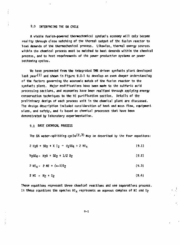
9.0 INTERFACING THE GA CYCLE

A viable fusion-powered thermochemical synfuels economy will only become reality through close matching of the thermal output of the fusion reactor to load demands of the thermochemlcal process. Likewise, thermal energy sources within the chemical process must be matched to heat demands within the chemical process, and to heat requirements of the power production systems or power bottoming cycles.

He have proceeded from the Integrated TMR driven synfuels plant developed last year'U and shown 1n Figure 9.0-1 to develop an even deeper understanding of the factors governing the economic match of the fusion reactor to the synfuels plant. Major modifications have been made to the sulfuric add processing sections, and economies have been realized through applying energy conservation techniques to the HI purification section. Details of the preliminary design of each process unit in the chemical plant are discussed. The design description included consideration of heat and mass flow, equipment sizes, and safety, and is based on chemical processes that have been demonstrated by laboratory experimentation.

9.1 BASE CHEMICAL PROCESS

The GA water-splitting eyelet 2' 3' may be described by the four equations:

2 H2O + SO2 + X I2 •* H2SO4 + 2 HI X (9.1)

H2SO4-* H2O • SO2 + 1/2 O2 (9.2)

2 HIX- 2 HI + (x-in2 19.3)

2 HI -* H2 + I2 (9.4)

These equations represent three chemical reactions and one separations process. In these equations the species HI X represents an aqueous complex of HI and 12

9-1

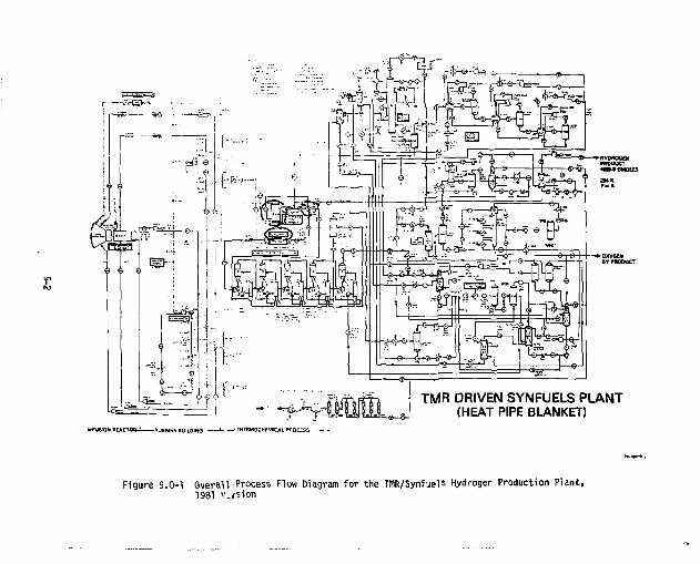
TMR DRIVEN SYNFUELS PLANT ^ (HEAT PIPE BLANKET)

W v S I O N BEACTOR-1- TURBINE BUILDING L TMERMOCMEM1CAL PBOCESS-

Figure 9.0-1 Overall Process Flow Diagram for the TMR/Synfueis Hydroger Production Plant, 1981 v.rsion

formed by reaction 1. The H2SO4 product of reaction 1 is obtained as a moderately concentrated aqueous solution which is immiscible with HI X-

The overall process is divided into five sections for design purposes Sections I through IV roughly correspond to the four equations and section V represents the heat and energy transmission equipment required to match the fusion heat source to the chemical process. Descriptions of sections I through IV occupy the remainder of section 9 of this report. Section V 1s described 1n report section 10.

The developmental effort on the GA Sulfur-Iodine cycle has proceeded since 1974 along three parallel and mutually supportive lines:

0 Chemical investigations 0 Engineering flowsheet development 0 Process demonstration

Chemical investigations are the basis for the engineering flowsheet development and process demonstration. Synergist!cally, the flowsheet development and process demonstration efforts give impetus and direction to further chemical investigations. Likewise, each of these tasks raises new questions in its own area.

9.2 RECENT DEVELOPMENTS IN PROCESS CHEMISTRY

The GA water-splitting process is not a static entity but is constantly being upgraded. Information has recently been made available on three chemical innovations to the process^.4), i„ addition, other new techniques have not yet reached the publication stage.

We have investigated one of the three techniques, HBr based HI purifica­tion^), but the initial energy balances are not favorable compared with the H3PO4 based HI purification process used In previous flowsheets. The other two techniques have been developed to the preliminary flowsheet stage under separate funding. HI decomposition via homogeneous catalysis'2) will

9-3

eventually be incorporated into the fusion synfuels design, but since HI decomposition is relatively inexpensive there is l i t t l e urgency. The Sulfur-Sulfuric Acid Chemical Energy Storage system^), developed for solar applica­t ions, has the potential for long-term energy storage. Long-term storage could benefit a fusion synfuel plant by permitting the synfael plant to maintain operation during scheduled and nonscheduled outing of the TMR. In addition, this system could provide on-site power for cold start-up of the TMR.

None of these process improvements have been included in this year's f inal

design.

Discussion of this year's design resumes with section 9.3

9.2.1 HBr Based HI Purifications*2> In the sulfur-iodin :ycle a solution of HI, Ig, and H2O is produced.

This solution is the latent source of H2 from the cycle. The HI and the H2O are present in this solution at partial molar free energies of -6.2 and -0.6 kcal/mole, respectively!5). In order to separate these components, at least these energies must be supplied. The cycle, in its current embodiment, uses concentrated H3PO4 to act on the solution in such a way that most of the iodine separates into a second phase and, more importantly, the chemical potential of the HgO is lowered by binding H2O in the influence sphere of the K3PO4. This results in enhancement of the chemical potential of HI to the degree that it can be separated from the H2O-H3PO4 solution by fractional distillation. Most of the energy associated with the HI-H2O-I2 solution separation is required during the separation of H2O from K3PO4 to prepare the H3PO4 for recycle. In the present engineering design of this portion of the process, this energy is supplied as work in the form of vapor recompression by turbines which take HgO vapor from the H3PO4 distillation and compress it, causing condensation and the concomitant release of the heat of vaporization at temperatures slightly higher than the heat used to evaporate the HgO in the first place. This vapor-recom-pression scheme saves considerable heat energy but uses expensive work energy generated in expensive equipment.

9-4

Because of the costs of processing and not because of energy efficiency considerations, other techniques for HI recovery from HI-H2O-I2 solutions have been investigated. Finding other competitive methods to rectify this solution is not any easy task. The energies involved are those of chemical reactions not usually encountered in solution separations. A simple extraction agent for HI must react with HI with greater energies than HI has with H2O-I2 systems. While one may find appropriate agents, the problem then becomes how to get the HI out of the extraction agent. A number of organic reagents which may extract HI reasonably well fall at this later stage. Nevertheless, success has been achieved in the search for alternate methods of processing HI-I2-H2O solutions.

In an ef.rller publication'6', HI and H2O mixtures were reported to form two liquid phases: (1) a nearly dry liquid HI, and (2} a strong superazeo-troplc solution of HI 1n H2O. Mixtures of HC1-H2U were also reported to phase separate'7'. This liquid-phase formation was concluded to have considerable value in separating HI from HI-I2-H2O product solutions from the H2O-SO2-I2 reaction. However', to achieve separation conditions, the HI content of these product solutions needs to be considerably increased. Up to now, this seemed possible only by techniques already in use, such as H3PO4 treatment.

Still earlier, a high-pressure distillation to break the HI-H2O-I2 pseudoazeotrope was Investigated'**' as an alternative to the H3PO4 tr atment. This distillation process was found to be considerably less efficient than breaking the azeotrope of HCI-H2O' 9}. Thus, the pursuit of this technique was temporarily abandoned. However, some engineering evaluations of the small azeotrope shifting, found to occur in the HI-K2O system (57* HI to^45£), indicated that this process is basically similar in efficiency to the H3PO4 treatment.

A process has been conceived which combines high-pressure azeotrope shifting, two-phase formation, solvent extraction using a hydrogen halide (HC1 or HBrS for HI separation, and some other features to sharply reduce the amount of H20 distilled in processing HI X solutions. To establish the feasibility of this process, laboratory experiments were undertaken to study (1) the distribution of HI between a dry hydrogen halide phase and the wet phase,

9-5

(2) the behavior of I2 in these phases, (3) the high-pressure distillation to separate H2O and HBr, (4) the fate of the HBr and the degree of reaction of the reactants in the H2O-SO2-I2 reaction, and (5) the recovery of HBr from these product solutions. The preliminary result of these studies was that an HBr based separation process had the potential for significant energy and capital savings over the HBr based process. The process flowsheets developed as part of this work did not demonstrate these potential savings. The flowsheet work is presented in section 9.6.

9.2.2 HI Decomposition Via Homogeneous Catalysis

The present version of the sulfur-iodine water-splitting process employs HI decomposition in the liquid phase. Theoretical calculations indicate that high conversion levels are possible using such a scheme, and indeed high conversions were verified experimentally^O). \n addition, the same article reports that the magnitude of extrapolated rate data to high process temperatures appears sufficient ti result in a viable process for HI composition. The above rate data were obtained by extrapolating measured rate data from lower temperatures and pressures in batch studies performed on supported platinum and ruthenium catalysts.

Recently, some data for a supported platinum catalyst at closer to actual engineering temperatures and pressures were obtained in a new flowing liquid HI bench-scale system. The rate value obtained gave credence to the use of the extrapolated lower temperature data and thus is verification of the present flowsheet and equipment sizing calculations.

Further in-depth studies, however, revealed a problem associated with the use cf heterogeneous catalysis to decompose liquid HI. This is associated with the finding that at least platinum, whether supported or not, does dissolve in the liquid HI to a non-negligible degree. This requires the use of some kind of catalyst recovery and remanufacture scheme. Catalyst recovery and remanufacture are commonplace in the chemical industry but add to the complexity and to the operational and capital costs of the overall process. It was due to the discovery of such an additional requirement of the process that

9-6

some consideration was given to the use of homogeneous catalysis to decompose HI and to potential separation schemes inherent in the practical application of homogeneous catalysis.

A homogeneous catalyst concept has been devised'2) in which there is an innate separation of the catalyst from the HI liquid, thereby allowing the catalyst to be totally recycled to the reactor. The concept is based on some unique findings surrounding the phase behavior of HI-Ig-HgO mixtures. For certain compositions of these three chemicals, two liquid phases in equilibrium can exist. One phase is a very dry phase of HI and I2; the other is an aqueous phase containing both Ig and HI. It has been found that it is in this latter phase that certain homogeneous catalyst compounds tend to concentrate. This means that the aqueous phase acts essentially as the catalyst carrier and can be recycled to the HI decomposition reactor without having to recover the catalyst.

The potential advantages over a process employing heterogeneous catalysts with the need to recover and remanufacture 100% of the catalyst are clear. The proposed homogeneous process has been conceptually flowsheeted {but at too late a date for inclusion in this overall process design) and major areas requiring investigation have been identified. The needed information consists mainly ir< identifying the solubility and distribution of the catalyst in the fluids of the process train at engineering conditions, determining the best area of the HI-I2-H2O phase diagram in which to work, and determining the best schemes for catalyst recycle. The results of this work have supported this concept as a viable engineering process.

9.2.3 The Sulfur-Sulfut'ic Acid Chemical Energy Storage System

A sulfur-sulfuric acid energy storage system has been proposed for the GA sulfur-iodine water-splitting cycle for use in conjunction with a solar heat source This storage system has the potential for reducing the cost of fusion produced synfuels. During steady state operation of the THR, a small amount of sulfuric acid could be converted to sulfur. During outages of the TMR, the sulfur could then be burned in air providing both the feed stock and

9-7

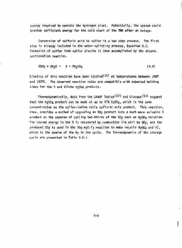
energy required to operate the hydrogen p lan t . Po ten t i a l l y , the system could provide s u f f i c i e n t energy for the cold s ta r t of the TMR a f te r an outage.

Conversion of s u l f u r i c acid to su l fu r is a two step process. The f i r s t step i s already included in the w a t e r - s p l i t t i n g process, Equation 9.2. Formation of su l fu r from su l fu r dioxide i s then accomplished by the d ispro-por t ionat ion reac t ion .

3S02 + 2H20 -<- S + 2H2SO4 (9.5)

K inet ics of t h i s react ion have been s t u d i e d ' 1 1 ' at temperatures between 100°

and 140°C. The observed react ion rates are compatible wi th expected holding

times fo r the S and d i l u t e H2SO4 products.

Thermodynamically, data from the JANAF Tab les ' 1 ^ ) a n c ) G iauque ' 1 3 ) suggest tha t the H2SO4 product can be made at up to 57% H2SO4, which i s the same concentration as the su l fu r - iod ine cycle s u f l u r l c acia product. This reac t ion , then, provides a method of upgrading an SO2 product in to a much more valuable S product at the expense of cyc l ing two- th i rds of the SO2 back as H2SO4 so lu t i on . The stored energy i n the S i s recovered by combustion ( i n a i r ) to SO2, and the produced SO2 is used in the SO2-H2O-I2 react ion to make recycle H2SO4 and H I , which is the source of the H;> in the cyc le . The thermodynamics of the storage cycle are presented in Table 9 . 2 - 1 ,

9-8

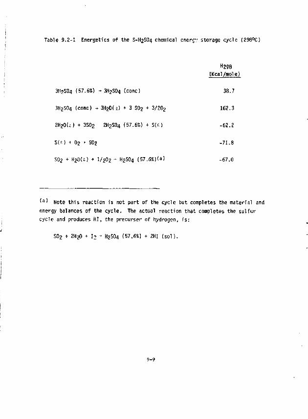
Table 9.2-1 Energetics of the S-H2SO4 chemical enerc." storage cycle (298°C)

H298 (Kcal/mole)

3K?S0fl (57.6%) -3H2S04 (cone) 38.7

3H2SO4 (cone) -> 3H20(a) + 3 SO? + 3/202 162.3

2H20(i) + 3S02 2H2SO4 {57.6%) + SU) -62.2

SU) + 0 2 - SO2 -71.8

SO2 + HjOfa) + I/2O2 •* H2SO4 (57.6*)(a) -67.0

( a ) Note this reaction is not part of the cycle but completes the material and energy balances of the cycle. The actual reaction that completes the sulfur cyc?e and produces HI, the precurser of hydrogen, fsr

SO2 + 2H2O + I2 - H2SO4 (57.6%) + 2HI (sol).

9-9

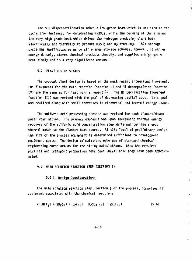
The SO2 disproportionate makes a low-grade heat which is utilized in the cycle (for instance, for dehydrating H2SO4K while the burning of the S makes the very high-grade heat which drives the hydrogen produci'n; plant both electrically and thermally to produce H2$04 and H2 from SO2. This storage cycle has inefficiencies as do all energy storage schemes; however, it stores energy densely, stores chemical products cheaply, and supplies a high-gr-»de heat simply and in a very significant amount.

9.3 PLANT DESIGN STATUS

The present plant design is based on the most recent integrated flowsheet. The flowsheets for the main reaction (section I) and HI decomposftion (section IV) are the same as for last year's report^). The HI purification flowsheet (section III) was revised with the goal of decreasing capital cost. This goal was realized along with small decreases in electrical and thermal energy usage.

The sulfuric acid processing section was revised for each blanket/decom­poser combination. The primary emphasis was upon increasing thermal energy recovery of the sulfuric acid concentration step while maintaining a good thermal match to the blanket heat, source. At this level of preliminary design the size of the process equipment is determined sufficient to development equipment costs. The design calculations make use of standard chemical engineering correlations for the sizing calculatJons. Hhen the required physical and transport properties have been unavailable they have been approxi­mated .

9.4 MAIN SOLUTION REACTION STEP (SECTION I)

9.4.1 Design Considerations

The main solution reaction step, Section I of the process, comprises all equipment associated with the chemical reaction:

2 ^ 1 ^ ) + S02(g) + l2<*2> H2SO4U1) + 2HI(£ 2) (9.6)

9-10

where gaseous sulfur dioxids reacts with an excess of molten iodine and water to produce two immiscible liquid phases. The designation 11 indicates that water is the major component in the H2SO4 product phase, and 4 2 t n a t iodine *s the major component in the HI product phase. The H2SO4 phase which is the lighter (lower density) phase, also contains a trace of iodine. The heavy phase, referred to as HI X, because it contains excess iodine in a complexed form, also contains water. The main solution reaction is exothermic and Section 1 requires no heat input from the fusion reactor but exports a significant quantity of low-grade heat to a power bottoming cycle. The Section I process is shown schematically in F'-gure 9.4-1.

Even though Section I requires no heat input from the fusion reactor, the design of the main solution reaction step has a major influence on the overall process efficiency and thus upon the reactor size and the hydrogen production cost. Although decisions on heat ar.d power recovery within Suction I have an effect on efficiency, the composition and temperature of the light phase flowing to process Section II (the H2SO4 processing step) and of the heavy phase flowing to Section III (the HI concentration step) strongly influence the overall efficiency of the process. In the interest of efficiency, both streams should leave Section I at as high a temperature as possible and at the highest acid concentration possible. Since the equilibrium of an exothermic reaction shifts towards the reactants as temperature is raised, a compromise must be made between high tetnperature and high acid concentrations in the product. In deciding the operating conditions for Section I some economic trade-off calculations were made but a full-scale process optimization was not in the scope of this work. The basis for the resulting decisions, as well as those for the rest of this study, may best be termed "engineering judgment." When trade-off calculations were not definitive, the decision was usually made on the side of "high efficiency" not "low capital cost."

Consideration of two factors dominates the design of Section I: (1) the large quantity of heat produced by th( main solution reaction must be removed, and (2) the combination of hydrogen iodide and iodine in the heavy aqueous phase is extremely corrosive to materials normally employed for heat transfer surfaces. The only metals known to rtsist HI X are refractory m.tals such as

9-U

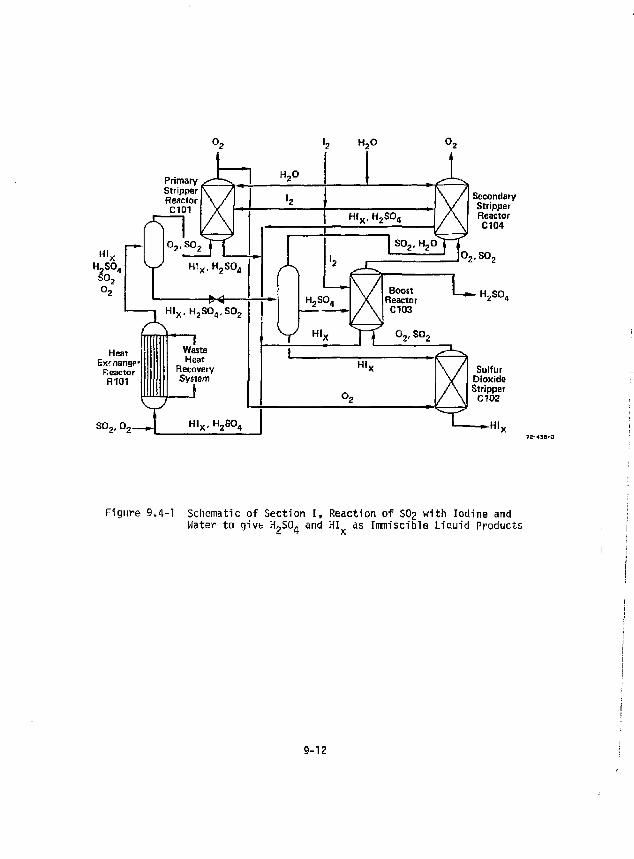
Secondary Stripper Reactor CI 04

Figure 9.4-1 Schematic of Section I, Reaction of SO2 with Iodine and Water to give H-SO. and HI as Immiscible Liquid Products

9-12

niobium, tantalum, and molybdenum. The present design employs niobium for heat transfer surfaces contacting HI X, which permits the reaction energy to be used in the power bottoming cycle.

Niobium is relatively expensive: therefore, to reduce the capital cost of Section I, a number of design techniques have been employed which Improve heat transfer and decrease the amount of Nb required. Some of these are:

1. Cool feed streams to Section I. Prior to carrying out the sain solution reaction, we transfer the heat from the Section I feed streams to the power bottoming cycle. This involves less expensive heat transfer materials than Nb and reduces the amount of heat transferred from the reaction products of the main solution reaction.

2. Operate adiabatically. Instead of cooling the reaction products from 393 to 368 K (to shift the equilibrium towards the products) and then reheating the separated products, we operate adiabatically, and maintain the desired production rate of the main solution reaction by increasing the iodine concentration to provide the needed shift in the equilibrium.

3. Use direct-contact heat exchange. Where possible, we employ direct contact heat exchange between immissible liquid phases or gas and liquid phases.

4. Apply enhanced heat transfer techniques. Utilizing two-phase gas-liquid flow through the heat exchanger gives higher than normal convective heat transfer coefficients. Spiral-fluted tubing provides enhanced heat transfer and, due to the wall stiffening effect, permits thinner tube walls.

9.4.2 Heat Exchanger Reactor

Almost 522 of the chemical reaction forming HI and H2SO4 takes place in the Heat Exchanger Reactor (R-101 in the flow diagram of Figure 9.4-1) and in

9-13

the plpfng Immediately preceeding the reactor. The reactor selected 1s a shell and tube heat exchanger with fixed tube sheets. The vessel, tube sheets, and heads are fabricated from mild steel. The heads are Tiaed with fluorocarbon and the splral-fluted niobium tubes are welded to a niobium tube sheet liner. The process fluid is on the tube side of the heat exchanger and the shell side is part of the power bottoming cycle.

Upstream of the heat exchanger, the SO2/O2 from Section II (sulfuric acid processing) is mixed with the predominantly iodine stream from the Boost Reactor (C-103) and aqueous streams from the scrubbing reactors {C-101 and C-104). The combined streams react exothermfcally as they flow through a fluorocarbon-lined pipe and into the heat exchanging reactor. The pressure drop through the heat exchanger reduces the system pressure from an initial 0.50 MPa to 0.44 MPa at which point the temperature reaches 393 K. At the exit of the heat exchanger the 02 is removed from the stream in the first of two separators (S-101). In the second separator (S-102), operating at 0.11 HPa, three phases separate: the heavy liquid phase (HI X), the light liquid p.ase (H2O/H2SO4), and a gas phase consisting of SO2 and steam. The vaporization of water and SO2 results in the temperature decreasing from 393 k to 385 K.

9,4.3 Lower Phase SOp Stripper

The lower phase solution (HI X) is saturated with SO2 which when allowed to remain forms sulfur and H2S via tramp reactions. An oxygen recycle stream strips most of *.h SO2 in a packed bed stripper (C-102) thus minimizing the tramp reactions. A minimum amount of oxygen is employed for this operation as the evaporation of water into the oxygen cools the HI X requiring more heat input in Section III (HI purification). With a 10S O2 recycle the KI X is cooled from 385 K to 381 K.

The stripper, sized for operation at 70S of flooding, is a standard packed column design. The fluorocarbon-lined mild steel vessel is packed with 50 mm ceramic Raschig rings. Since the operating pressure is near atmospheric, a glass-lined steel vessel is a viable option but would require fluorocarbon packing to avoid liner damage.

9-H

9.4.4 Boost Reactor

In the boost reaction, the sulfuric acid concentration of the light phase is increased from 502 to 57S by contacting with molten iodine v'n the presence of sulfur dioxide. The increased H2SO4 concentration 1s realized through the action of the main solution reaction. Water is used up by reaction with SO2 and I2 to form H2SO4 and HI. Over 7% of the total chemical reaction of Section I occurs in the Boost Reactor. Since the contact is performed in a counter-current manner, the reactor also acts as a direct contact heat exchanger, raising the temperature of the sulfuric acid stream from 383 K to 393 K.

Although the mechanical design of the Boost Reactor is straightforward, i.e., a fluorocarbon-lined mild steel vessel packed with 50 mm ceramic Raschig rings, the sizing calculations are not. Common packed columns operate with either a gas rising through a decending liquid phase, or a light liquid phase rising through a decending heavy liquid phase. The Boost Reactor has both a gas phase (SO2 in O2) and a light liquid phase (H2SO4 6'td water) rising through the decending heavy liquid phase {I2). The present design is based on adding the cross-sectional areas required if the gas and light liquid separately contacted the heavy liquid. This is a very conservative approach. We believe that a design based upon information gained 1n a pilot plant would result in a smaller Boost Reactor vessel.

9.4.5 Scrubbing Reactors

The oxygen is purified before discharge to the atmosphere in the Scrubbing Reactors. The packed column reactors operate in a titration mode in which sufficient iodine is added to the scrub water in the lower part of the column to react stoichiometrically with the sulfur dioxide present in the oxygen. In the upper part of the column the oxygen is washed with pure water. The primary Scrubbing Reactor (C-101) operates at 0.44 MPa purifying the gaseous product of the Heat Exchanger Reactor (R-101). Over 192 of the Section I reaction takes place in the primary Scrubbing Reactor. Almost 22* of the total reaction takes place In the secondary Scrubbing Reactor at 0.10 HPa. The secondary scrubber cleans up the oxygen stream exiting the Boost Reactor as well as the steam/S02

9-15

stream produced during depressurization of the liquid reaction product of the Heat Exchanger Reactor.

Both scrubbing reactors perform a second function as direct contact heat exchangers. Oxygen leaving the process is cooled to near ambient conditions while preheating the water entering the process. The scrubber vessels are of fluorocarbon-lined mild steel and the packing is 50 mm ceramic Raschig rings. Pilot plant tests may demonstrate reduced vessel costs. The upper portions of the scrubber contain only water and oxygen so no lining should be required in this area. Depending upon the temperatures reached in the lower portions of the scrubber, less expensive linings may be possible.

9.4.6 Heat and Power Recovery

The heat transferred to the steam power bottoming cycle from Section 1 totals 782 MWt. The majority of this is transferred via the Heat Exchanger Reactor but significant quantities of heat are also transferred from the hot water products of Sections II and III and from the SO2/O2 product of Section II. Since the heat transfer materials used for water and SO2 are much less expensive than the niobium used in the Heat Exchanger Reactor, there 1s the potential for further cost reduction by performing more of the cooling on water and SO2 streams. Ultimately an economic optimization must determine the split in heat transfer duties on the basis of minium hydrogen production cost.

A total of 5.4 KW is recovered in Section I using turbines for pressure reduction. Preliminary indications are that the turbines ^re economic but a final determination must await an analysis based on the hydrogen production cost resulting from this study.

9-5 H ?S0 4 PROCESSING STEP (SECTION II)

9.5.1 Design Considerations

The sulfuric acid processing step, Section II of the process, takes 57$ H2SO4 from Section I, decomposes the H2SO4 and returns the resulting SO2,

9-16

02, and H2O back to Section I. Process flow diagrams are given in Figures 9.5-1 and 9.5-2 for the Joule Boosted and Fluid Bed versions of the process.

Major unit operations of Section II are sulfuric acid concentration, vaporization, and decomposition. Vaporization and decomposition equipment designs are based on last year's report, but the sulfuric acid concentration section has been completely re-flowsheeted.

In the interest of capital cost savings, last year's flowsheet left out the vapor recompression equipment which were part of the original GA designl^). j n e process efficiency reported by GA (47$) cannot be achieved without recovering a large fraction of the heat of vaporization of the water accompanying the sulfuric acid. These new flowsheets accomplish this goal without resorting to vapor recompression techniques.

9.5.2 A d d Concentration

Several techniques were tri^J to accomplish the goal of heat recovery without vapor recompression. These included multi-effect evaporators, pressure staged flash evaporators (adlabatic an>1 non-adiabatic) and column evaporators. It became evident that no single technique could achieve the desired goal. A combination of four different concentration techniques was used in the final flowsheet.

Staged isobaric boiling at 7.5 MPa was used to achieve the goal of water removable at useful steam temperatures. Atmospheric distillation was used for final concentration of the acid to the azeotropic composition. A single adiabatic flash stage at 1.1 MPa was used to match the isobaric staged boiling to the atmospheric distillation column. Finally, staged partial condensation was used to remove H2SO4 from the decomposed product along with a minimum of water.

The Isobaric staged boiling is accomplished in what can be described as a horizontal distillation column. The design 1s patterned after the H2SO4 vaporizer described in last year's report and shown in Figure 9.5-3. The

9-17

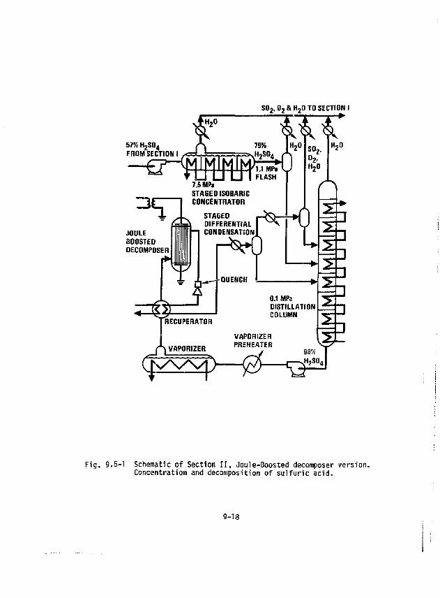
S0 2 , 0 2 & H 2 0 TO SECTION I

57% H 2 S0 4

FROM SECTION)

< ^ — $ s > — ^

Fig. 9.5-1 Schematic of Section II, Joule-Boosted decomposer version. Concentration and decomposition of sulfuric acid.

9-18

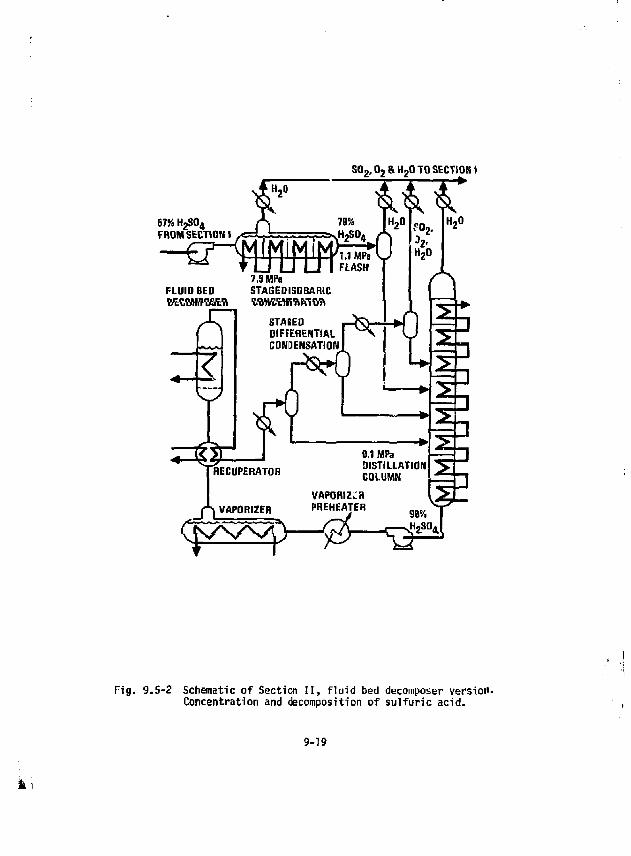
S 0 2 , 0 2 & H 2 0 TO SECTION t

87% H 2 S0 4

FROM SECTION I

£^Z^ ^

Fig. 9.5-2 Schematic of Section II, fluid bed decomposer versiot'. Concentration and decomposition of sulfuric acid.

k

9-19

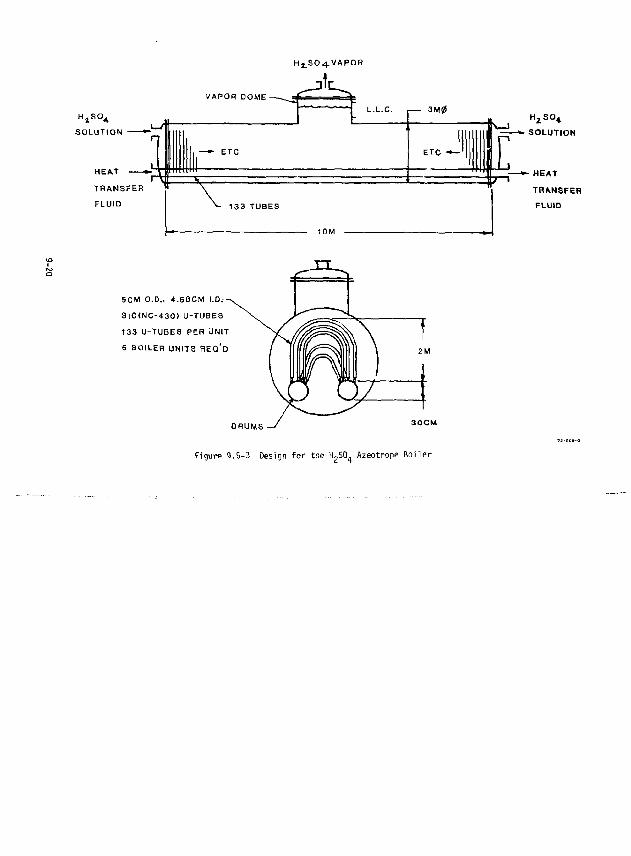
SOLUTION

HEAT •

TRANSFER

FLUID

H ^ S O ^ - V A P O R

tr VAPOR DOME

ETC

133 TUBES

^ L.L.C. , 3 M 0

10M

ETC J S—1

E H 2 S 0 4

SOLUTION

• HEAT

TRANSFER

FLUID

5CM O.D., 4 .68CM I.D.

S lC<NC-430) U-TUBES

133 U-TUBES PER JNIT

S BOILER UNITS R E Q ' D

DRUMS•

Figure 9.5-3 Design f o r the lUSO. Azeotrope B o i l e r

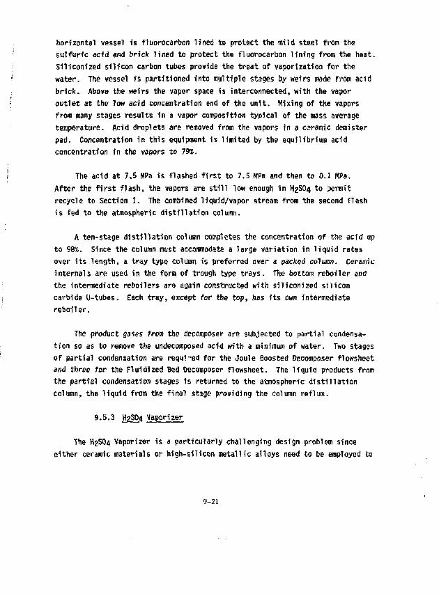
horizontal vessel Is fluorocarbon lined to protect the mild steel from the sulfuric acid and brick lined to protect the fluorocarbon lining front the heat. Siliconized silicon carbon tubes provide the treat of vaporization for the water. The vessel is partitioned into multiple stages by weirs made from acid brick. Above the weirs the vapor space is interconnected, with the vapor outlet at the low acid concentration end of the unit. Mixing of the vapors from many stages results in a vapor composition typical of the mass average temperature. Acid droplets are removed from the vapors in a ceramic demister pad. Concentration In this equipment is limited by the equilibrium acid concentration in the vapors to 79%.

The acid at 7.5 MPa is flashed first to 7.5 MPa and then to 0.1 MPa. After the first flash, the vapors are still low enough 1n H2SO4 to permit recycle to Section I. The combined liquid/vapor stream from the second flash is fed to the atmospheric distillation column.

A ten-stage distillation column completes the concentration of the acid up to 98%. Since the column must accommodate a large variation in liquid rates over its length, a tray type column is preferred over a packed column. Ceramic internals are used in the form of trough type trays. The bottom reboiler and the intermediate reboilers are again constructed with siliconized silicon carbide U-tubes. Each tray, except for the top, has its own intermediate reboiler.

The product gases from the decomposer are subjected to partial condensa­tion so as to remove the undecomposed acid with a minimum of water. Two stages of partial condensation are requi-ed for the Joule Boosted Decomposer flowsheet ana three for the Fluidized Bed Decomposer flowsheet. The liquid products from the partial condensation stages is returned to the atmospheric distillation column, the liquid from the final stage providing the column reflux.

9.5.3 H2J&4 Vaporizer

The H2SO4 Vaporizer is a particularly challenging design problem since either ceramic materials or high-silicon metallic alloys need to be employed to

9-21

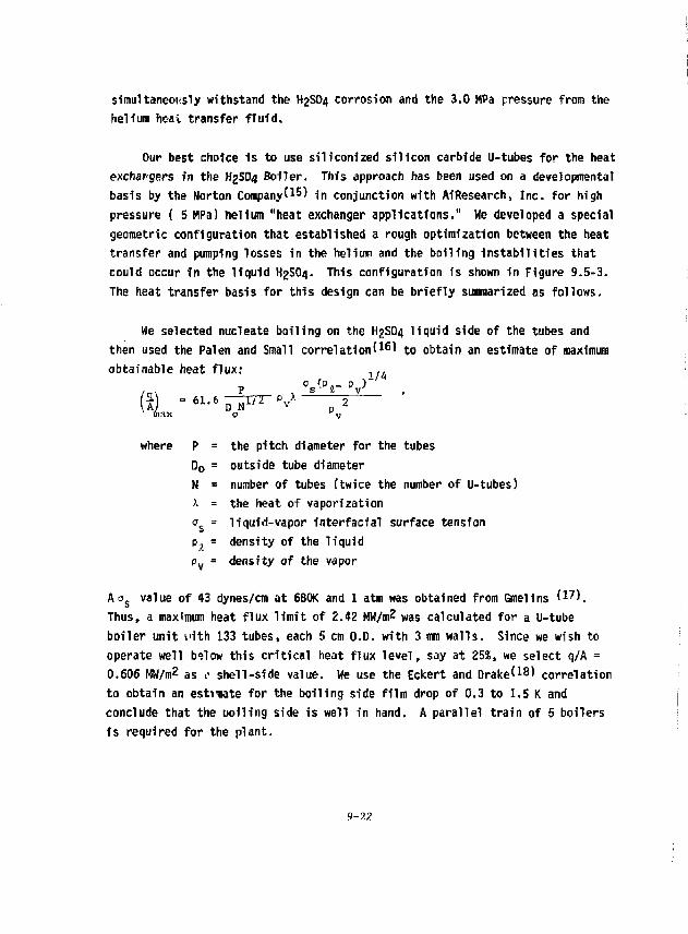
simultaneously withstand the H2SO4 corrosion and the 3.0 MPa pressure from the helium hc-ai transfer fluid.

Our best choice is to use siliconized silicon carbide U-tubes for the heat exchangers in the H2SO4 Boiler. This approach has been used on a developmental basis by the Norton Company^ 1 5) in conjunction with AiResearch, Inc. for high pressure ( 5 HPa) helium "heat exchanger applications." He developed a special geometric configuration that established a rough optimization between the heat transfer and pumping losses in the helium and the boiling Instabilities that could occur in the liquid H2SO4. This configuration is shown in Figure 9.5-3. The heat transfer basis for this design can be briefly summarized as follows.

We selected nucleate boiling on the H2SO4 liquid side of the tubes and then used the Palen and Small correlation^ 1 6) to obtain an estimate of maximum obtainable heat flux: ,,,

f ) = 6 1 . 6 ^ I 7 ^ P V > p 2 max o K v

where P = the p i tch diameter fo r the tubes

D 0 = outside tube diameter U = number of tubes (twice the number of U-tubes) x = the heat of vapor izat ion o = l iqu id -vapor i n t e r f a c i a l surface tension Pj, = densi ty of the l i q u i d P V = densi ty of the vapor

A o s value of 43 dynes/cm at 680K and 1 atm was obtained from Gmelins f ^ ) . Thus, a maximum heat f l u x l i m i t of 2.42 MW/m? was calculated f o r a U-tube b o i l e r u n i t t ' i t h 133 tubes, each 5 cm O.D. wi th 3 mm w a l l s . Since we wish to operate well below t h i s c r i t i c a l heat f l u x l e v e l , say at 25%, we select q/A = 0.606 MW/m2 as c» she l l -s ide value. We use the Eckert and Drake^ 1 8 ) co r re la t ion to obtain an es tmate for the bo i l i ng side f i l m drop of 0.3 to 1.5 K and conclude that the p o l l i n g side i s well in hand. A para l l e l t r a i n of 5 bo i le rs is required for the plant.

9-22

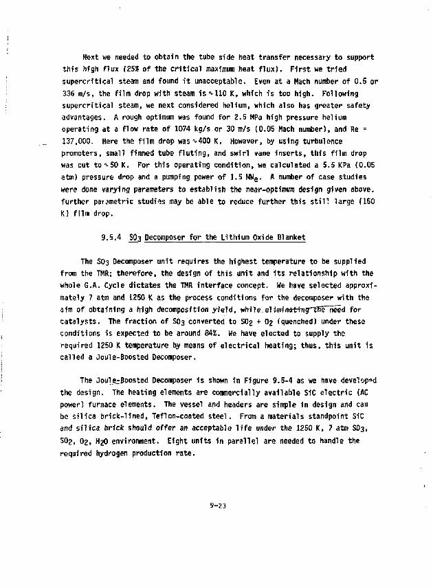
Next we needed to obtain the tube side heat transfer necessary to support this high flux (252 of the critical maximum heat flux). First we tried supercritical steam and found it unacceptable. Even at a Hach number of 0.5 or 336 m/s, the film drop with steam is^llO K, which is too high. Following supercritical steam, we next considered helium, which also has greater safety advantages. A rough optimum was found for 2.5 MPa high pressure helium operating at a flow rate of 1074 kg/s or 30 m/s (0.05 Mach number), and Re = 137,000. Here the film drop was 400 K. However, by using turbulence promoters, small finned tube fluting, and swfrl vane inserts, this film drop was cut to T-50 K. For this operating condition, we calculated a 5.5 KPa (0.05 atm) pressure drop and a pumping power of 1.5 MU e. A number of case studies were done varying parameters to establish the near-optimum design given above, further parametric studies may be able to reduce further this stll? large (150 K) film drop.

9.5.4 SO3 Decomposer for the Lithium Oxide Blanket

The SO3 Decomposer unit requires the highest temperature to be supplied from the TMR; therefore, the design of this unit and its relationship with the whole G.A. Cycle dictates the TMR interface concept. We have selected approxi­mately 7 atm and 1250 K as the process conditions for the decomposer with the aim of obtafning a high decomposition yield, while.eliwfnatfngTnTTieid for catalysts. The fraction of SO3 converted to SO2 + O2 (quenched) under these conditions is expected to be around 84%. We have elected to supply the required 1250 K temperature by means of electrical heating; thus, this unit is called a Joule-Boosted Decomposer.

The JoulerBoosted Decomposer is shown in Figure 9.5-4 as we have developed the design. The heating elements are commercially available S1C electric (AC power) furnace elements. The vessel and headers are simple in design and can be silica brick-lined, Teflon-coated steel. From a materials standpoint SiC and silica brick should offer an acceptable life under the 1250 K, 7 atm SO3, SO2, O2, H2O environment. Eight units in parallel are needed to handle the required hydrogen production rate.

9-23

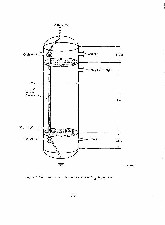
A.C. Power

Coolant - * ,

3 m 0

SiC Heating Elfimenl -

SO,

—»• Coolant

Coolant -—,

0.5 M

— » - S 0 2 + 0 2 + H 2 0

3 M

Coolant 0.5 M

F igu re 9 . 5 - 4 Design f o r the Jou le -Boos ted SO, Decomposer

9-24

Th? Joule-Boosted Decomposer of fers the best possible safety i so la t i on of the 02-containing process gases from the hot , l i q u i d metal-containing fusion blanket.

9.5.5 SO3 Decomposer fo r the Two-Zone Blanket

For the Two-Zone blanket, the decomposer is a ca ta l y t i c f l u i d i zed bed reactor operating at 1050-1100 K. The uni t contains in ternal heat exchanger tubes to provide the iieat for the highly endothermic SO3 •decomposition. I t can achieve up to a 55% conversion using 1 CuO ca ta l ys t , i f su l fa t ion of the cata lyst does not become a problem around 1U50-1100 K. I f su l fa t ion presents a serious problem, our a l te rna t ive is to use a more expensive platinum cata lys t on a t i t a n i a support. The deta i ls of th is Fluidized Bed Decomposer were given in the 19R0 Annual Report(19 , s"" only a b r ie f overview is provided here.

Figure 9.5-5 shows some of the deta i ls of the f l u id i zed bed design, using 0.5 mm diameter cata lyst spheres. The f l u id i zed bed i s on the shell side of the un i t with the helium on the tube side. The i ' fs across the helium f i l m w i th in the tube are about 20 K, and t h e i T s on the outside of the tubes in the f l u i d i zed bed region are expected to be around 14 K. The heliumAT presents a d i f f i c u l t design problem and the 20 K is a compromise between higher helium source temperatures and helium pressure.

The Fluidized Bed Decomposer requires seven units in para l le l to handle the needed production ra te . This approach of coupling the blanket to the process wi th helium of fers good safety i so la t i on for the process. More opt imizat ion work is needed to reduce tne overal l cap i ta l and operating costs f u r t he r . This concept saves the costs of a large tu rbo-e lec t r i c generator required in the Joule-Boosted Decomposer, at the expense of running a hotter fusion blanket and a more complex decomposer design.

9.5.6 Decomposer Recuperator

The Decomposer Recuperator is a heat exchanger un i t that simultaneously preheats the feed to the decomposer using heat from the hot SO2, O2, H2O, and

9-25

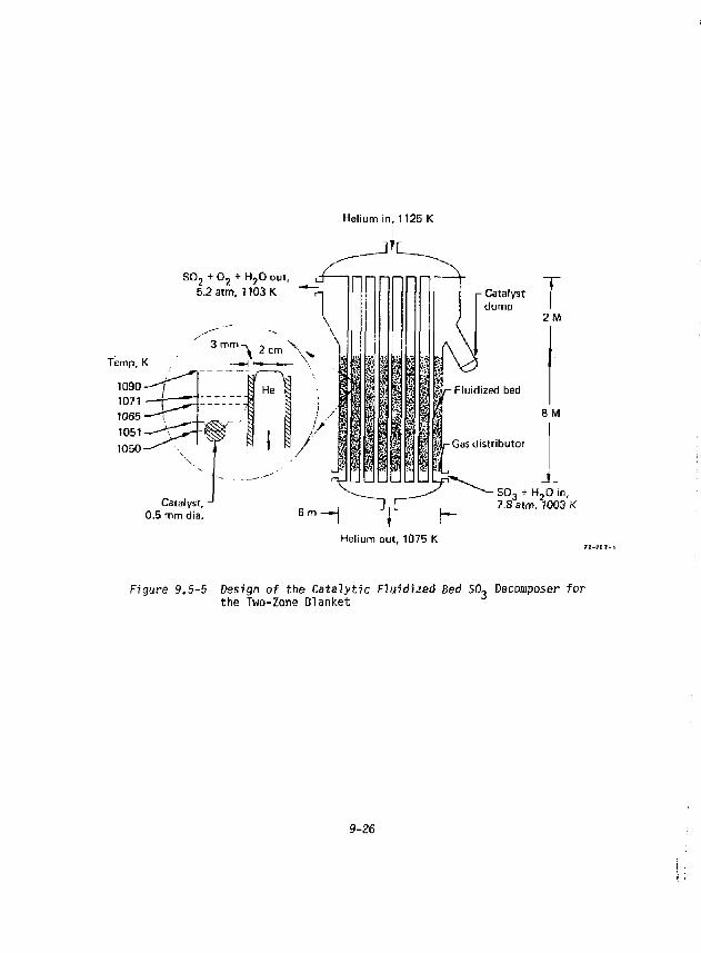
Helium in, 1125 K

Temp, K

S 0 2 + 0 2 + H 2 0 out, 5.2 atm, 1103 K Catalyst

dump T 2M

8 M

Catalyst, 0.5 mm dia.

H 7.8"atm,

2 0 i n , 1003 K

Helium out, 1075 K

F i g u r e 9 . 5 - 5 Design o f t h e C a t a l y t i c F l u i d i z e d Bed SO, Decomposer f o r t h e Two-Zone B lanke t

9-26

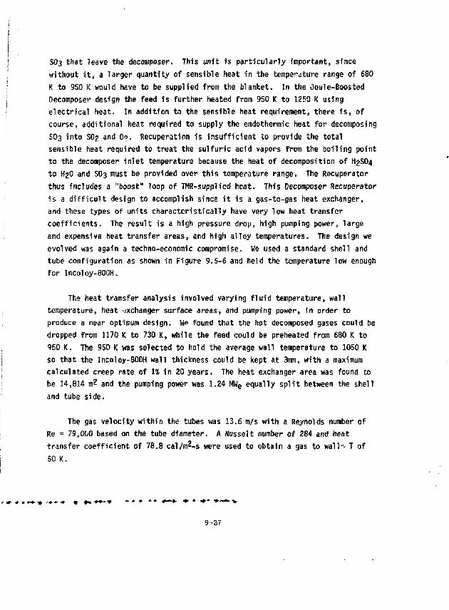
SO3 that leave the decomposer. This unit is particularly important, since without i t , a larger quantity of sensible heat in the tempe^ture range of 680 K to 9S0 l< would have to be supplied from the blanket. In the Joule-Boosted Decomposer design the feed is further heated from 950 K to 1250 K using electrical heat. In addition to the sensible heat requirement, there i s , of course, additional heat required to supply the endothermic heat for decomposing SO3 into SO2 and 0?. Recuperation is insufficient to provide the total sensible heat required to treat the sulfuric acid vapors from the boiling point to the decomposer inlet temperature because the heat of decomposition of H2SO4 to H2O and SO3 must be provided over this temperature range. The Recuperator thus includes a "boost" loop of THR-supplied heat. This Decomposer Recuperator is a d i f f i cu l t design to accomplish since i t is a gas-to-gas heat exchanger, and these types of units characteristically have very low heat transfer coefficients. The result is a high pressure drop, high pumping power, large and expensive heat transfer areas, and high alloy temperatures. The design we evolved was again a techno-economic compromise. We used a standard shell and tube configuration as shown in Figure 9.5-6 and held the temperature low enough for Incoloy-800H.

The heat transfer analysis involved varying f lu id temperature, wall temperature, heat exchanger surface areas, and pumping power, in order to produce a near optimum design. We found that the hot decomposed gases could be dropped from 1170 K to 730 K, while the feed could be preheated from 680 K to 950 K. The 950 K was selected to hold the average wall temperature to 1050 K so that the Incoloy-800H wall thickness could be kept at 3mm, with a maximum calculated creep rate of 1% in 20 years. The heat exchanger area was found to be 14,814 m2 and the pumping power was 1.24 MWe equally sp l i t between the shell and tube side.

The gas velocity within the tubes was 13.6 m/s with a Reynolds number of Re = 79,000 based on the tube diameter. A Nusselt number of 284 and heat transfer coefficient of 78.8 cal/m^-s were used to obtain a gas to wall^ T of 50 K.

9-27

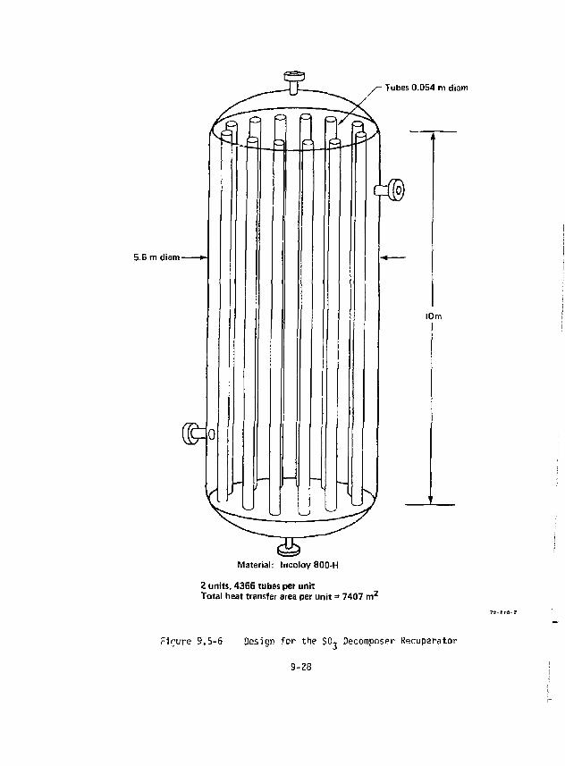
Tubes 0.054 m diam

5.6 m diam *•

Material: IncoloySOO-H

2 units, 4366 tubes per unit Total heat transfer area per unit = 7407 m 2

Figure 9.5-6 Design for the SO, Decomposer Recuperator

9-28

9.5.7 Decomposer Coolers

The Decomposer Cooler continues cooling the decomposer product after recuperation is no longer possible. Heat removed in the decomposer coolers is supplied to the atmospheric still and the multistage isobaric flash preheater. Sulfuric acid condenses out as the decomposer products are cooled. This sulfuric acid is removed in several stages, twice for the Joule-Boosted Decomposer case and three times in the case of the Fluid Bed Decomposer. The liquid phase from the final cooler is predominantly water; therefore, it is returned to Section I along with the gases.

Silicon carbide is required where sulfuric acid is condensing. At high temperatures, before the onset of condensation, Incoloy 800H would suffice except that silicon carbide is required for boiling sulfuric acid duty on the cold side of the tubes. After the majority of the sulfuric acid has been condensed and decanted, more conventional materials of construction are permitted. In the low temperature region the requirements of heating 57£ sulfuric acid demonates the material selection.

9-6 HI CONCENTRATION VIA HBR EXTRACTION-CASE STUDY (SECTION III)

9.6.1 Design Considerations

A first cut flowsheet was made for HI concentration via liquid HBr extraction* 2). The design goal was to separate HI from the HI X product of Section I in a cost effective manner. The flow diagram which resulted is shown in Figure 9.6-1. The design easily met the goal of low capital cost, but energy conservation in this new system has not progressed to the point where it can challenge the phosphoric acid based separation process.

9.6.2 HBr Extraction System

The HBr extraction (XC305) may be viewed as a traditional solvent extraction system employing partially miscible solvents. The two solvents HBr and H2O counter currently contact each other in either a packed or plate type

9-29

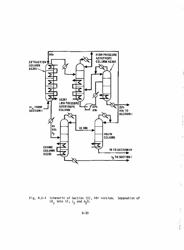
EXTRACTION!r

COLUMN XC305

25K HBr TO SECTION I

IODINE COLUMN XC3D3

HI TO SECTION IV

l 2 TO SECTION I

Fig. 9.6-1 Schematic of Section I I I , HBr version. H I X into HI, I 2 and H^fi.

Separation of

9-30

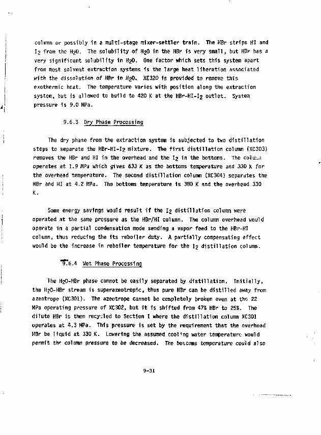
column or possibly in a multi-stage mixer-settler train. The HBr strips HI and 12 from the H2O. The solubility of H2O in the HBr fs very small, but HBr has a very significant solubility in H2O. One factor which sets this system apart from most solvent extraction systems is the large heat liberation associated with the dissolution of HBr in H2O. XE320 is provided to remove this exothermic heat. The temperature varies with position along the extraction system, but is allowed to build to 420 K at the HBr-HI-l2 outlet. System pressure is 9.0 HPa.

9.6.3 Dry Phase Processing

The dry phase from the extraction system is subjected to two distillation steps to separate the HBr-HI-I? mixture. The first distillation column (XC303) removes the HBr and HI in the overhead and the Ig in the bottoms. The colu;:„i operates at 1.9 MPa which gives 633 K as the bottoms temperature and 330 K for the overhead temperature. The second distillation column (XC304) separates the HBr and HI at 4,2 MPa. The bottoms temperature is 380 K and the overhead 330 K.

Some energy savings would result if the 12 distillation column were operated at the same pressure as the HBr/HI column. The column overhead would operate in a partial condensation mode sending a vapor feed to the HBr-HI column, thus reducing the its reboiler duty. A partially compensating effect would be the increase in reboiler temperature for the Ig distillation column.

*9*T6.4 Wet Phase Processing

The H20-HBr phase cannot be easily separated by distillation. Initially, the H20-HBr stream is superazeotropic, thus pure HBr can be distilled away from azeotrope (XC301). The azeotrope cannot be completely broken even at tho 22 MPa operating pressure of XC302, but it is shifted from 47% HBr to 253. The dilute HBr is then recycled to Section I where the distillation column XC301 operates at 4.3 HPa. This pressure is set by the requirement that the overhead HBr be liquid at 330 K. Lowering the assumed cooUng water temperature would permit th? column pressure to be decreased. The boitoms temperature could also

9-31

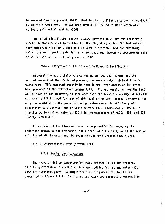
be reduced from its present 546 K. Heat to the distillation column is provided by multiple reboilers. The overhead from XC302 is fed to XC301 which also delivers substantial heat to XC301.

The final distillation column, XC302, operates at 22 MPa and delivers a 25$ HBr bottoms product to Section 1. The HBr, along with sufficient water to form azeotrope (483 HBr), acts as a diluent in Section 1 and the remaining water is free to participate in the prime reaction. Operating pressure of this column is set by the critical pressure of HBr.

9.6.5 Energetics of HBr Extraction Based HI Purification

Although the net enthalpy change was quite low, 132 k]/mole H2, the present version of the HBr based process, has excessively high heat flow to waste heat. This can most readily be seen in the large amount of low-grade heat produced in the extraction column XC305. 470 tcJ, resulting from the heat of solution of HBr in water, is liberated over the temperature range of 420-330 K. There is little need for heat of this quality in the . -ocess; therefore, its only use would be in the power bottoming system where its efficiency of conversiof to electrical energy wou""d be very low. Additionally, 190 kj is transferred to cooling water at 330 K in the condensers of XC301, 303, and 304 (mostly from XC301).

An analysis of the flowsheet shows some potential for reducing the condenser losses to cooling water, but a means of efficiently using the heat of solution of HBr in water must be found to make this process step viable.

9,7 HI CONCENTRATION STEP (SECTION III)

9.7.1 Design Considerations

The hydroyt;. iodide concentration step, Section III of the process, entails separation of a mixture cf hydrogen iodide, iodine, and water (HI X) into its component parts. A simplified flow diagram of Section III is presented in Figure 9.7-1. The iodine and water are separately returned to

9-32

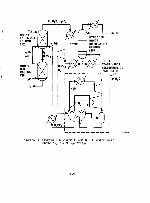
HI. H 2 0 , H 3 P 0 4

IODINE KNOCK-OOT COLUMN C302

H3PO4 H 20

IODINE WASH COLUMN C301

HI HYDROGEN IODIDE DISTILLATION COLUMN C303

[0X@p THREE STAGE VAPOR RECOMPRESSION EVAPORATOR

I

Figure 9.7-1 Schematic Flow Diagram of Section III, Separation of Aqueous HI into HI, lg, and H 20

9-33

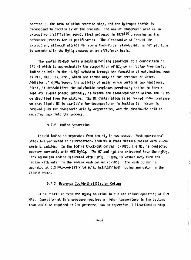
Section I, the main solution reaction step, and the hydrogen iodide is decomposed in Section IV of the process. The use of phosphoric acid as an extractive distillation agent, first proposed in

1975(20). remains as the

reference process for HI purification. The alternative of liquid HBr extraction, although attractive from a theoretical standpoint, is not yet able to compete with the H3PO4 process on an efficiency basis.

The system HI-H2O forms a maximum boiling azeotrope at a composition of 572 HI which is approximately the composition of H I X on an iodine free basis. Iodine is held in the HI-HgO solution through the formation of polyiodides such as HI3, HI5, HI7, etc., which are formed only in the presence of water. Addition of H3PO4 lowers the activity of water which performs two functions; first, it destabilizes the polyiodfde complexes permitting iodine to form a separate liquid phase; secondly, it breaks the azeotrope which allows the HI to be distilled from the mixture. The HI distillation is performed under pressure so that liquid HI is available for decomposition in Section IV. Water is removed from the phosphoric acid by evaporation, and the phosphoric acid is recycled back into the process.

9.7.2 Iodine Separation

Liquid iodine is separated from the HI X in two steps. Both operational steps are performed in fluorocarbon-lined mild steel vessels packed with 20-mro ceramic saddles. In the iodine knock-out column (C-302), the HI X is contacted counter-currently with 96? H3PO4. The HI and H2O are extracted into the H3P0d, leaving molten iodine saturated with H3PO4. H3PO4 is washed away from the iodine with water in the iodine wash column (C-301). The wash column is operated at 0.3 MPa-5irt-3$3"K td Ss'tc itetnt&iVtath iodine and water in the l iquid state.

9.7.3 Hydrogen Iodide Dist i l la t ion Column

HI is d is t i l led from the H3PO4 solution in a plate column operating at 0.9 MPa. Operation at this pressure requires a higher temperature in the bottoms than would be required at low pressure, but an expensive HI liquefaction step

9-34

is eliminated. Efficient use of the thermal energy, required for operation of the HI Distillation Column, is made possible by producing the HI product as a liquid and thus eliminating the thermodynamic inefficiency associated with a liquefactions compressor and that associated with production of power to operate it. Additionally, an intermediate condenser allows part of the condensing heat to be withdrawn from the column at a useful temperature. Although a majority of the heat required to preheat the feed and to operate the column is obtained by heat recovery within Section III, 355 MW is required from Section V at 523 K.

Design of the HI Distillation Column entailed a trade-off between capital and operating costs. Use of an intermediate condenser and operation at a relatively low reflux ratio reduce thermal energy requirements, but require more trays in the column for adequate chemical separation. The final design included 50 Hastelloy-C trays in a Hastelloy-C clad mild steel tower. The trays selected were the trough type, being a reasonable compromise between the higher efficiency, higher cost of bubble cap trays and the lower efficiency., lower cost of sieve trays.

An additional small design complication arises because the feed to the HI Distillation Column 1s saturated with iodine. Liquid iodine must be removed continuously from the middle of the column to avoid buildup. A stream, con­taining two liquid phases consisting of phosphoric acid and liquid iodine, is withdrawn from the iodine buildup region. The phosphoric acid returns to the column from the top of a liquid-liquid separator and the bottom iodine phase passes to the iodine wash column for phosphoric add removal before returning to Section I.

The small quantities of H2SO4 and SO2, remaining in the lower phase product from Section I, react chemically with HI in the feed preheater for the HI Distillation Column. The product of the reactions are H2O, I2, H2S, and S. The quantities involved are so small that the relative amounts of S and H2S have not been determined. For flowsheeting and cost estimating purposes, it has been assumed that half the sulfur in H2SO4 and SO2 ends up as HjS and half as S. The H^S will leave the column in the overhead product and the S 1s

9-35

assumed to exit tfie column wftfi the 1T3P04. TTie rfquftf S is separated from the H3PO4 and oxidized back to SO2 in Section II.

9.7.4 Phosphoric Acid Concentration

Removal of water from the phosphoric acid is accomplished in three stages of vapor recompression-driven flash evaporation. The operating condition of each stage has been modified so as to reduce capital cost for he{.t exchange-Each itage now operates at a different pressure with the pressure decreasing as the acid concentration increases. The major cost saving came through elimination of the heat exchanger which conditioned the evaporator feed. Only the first and last stages require any heat input from the fusion reactor, but all three stages require significant quantities of power for vapor recompres-sion. A tots) of £4J WW of shaft power is required to operate OJB compressors whereas only an additional 104 MW of thermal power at 484 K is required from Section V to heat the high temperature evaporator. Heat is recovered within each evaporation stage from interstage cooling of the six-stage tompressor, from the condensation of the compressed steam and from the concentrated phosphoric acid product.

The phosphoric acid concentration step is simple in concept but capital costs of the turbine compressors and heat exchangers are significant in the overall hydrogen production cost. Even though a considerable reduction in the cost of H3PO4 concentration has been made, alternative chemical systems are under continuing investigation with the goal of eliminating H3P0q from the process.

9.8 HI DECOMPOSITION STEP (SECTION IV)

9.8.1 Design Considerations

The HI decomposition step (Section IV of the process) requires the following operations:

0 Decompose HI(1) to H2(g) and Ig(l}

9-36

o Separate HI from the I2 and recycle to the decomposer 0 Separate HI from the H2 and recycle to the decomposer 0 Scrub the H2 product in preparation for distribution

A simplified schematic flow diagram of Section IV is presented in Figure 9.8-1.

Three process variables dominate the design of Section IV and have a direct impact on the fusion reactor interface. The temperature and pressure of the HI Decomposition Reactor govern the equipment size and amount of recycle through the reactor, whereas the HI-I2 Distillation Column pressure determines the maximum process temperature required from the fusion reactor. Variables governing the cleanup of the hydrogen product have a smaller, but still significant, impact on the hydrogen production cost.

9.8.2 HI Decomposition

Hydrogen iodide decomposition is accomplished in the HI Decomposition Reactor (R-401). The extent of the decomposition reaction is limited by thermodynamic equilibrium. Therefore, to limit the amount of recycle of HI back through the reactor, process conditions must be chosen so as to give a high conversion per pass through the reactor. Previous studies at the General Atomic Company^) n a V e demonstrated that when decomposition is carried out under high pressures so that HI and I2 are present as liquids, J much higher decomposition yield is obtained than with the analogous gas phase decomposition. Selection of the temperature and pressure involve a number of tradeoffs. The critical temperature of HI places an upper limit upon the Initial reaction temperature of an adiabatic flow reactor, while the required hydrogen delivery pressure places a lower bound upon the system pressure.

For this system design we still rely upon an adiabatic flow reactor using an activated charcoal catalyst. The recently developed homogeneous catalysis concept'2) became available after this year's design base was fixed.

The reactor was sized for a 4-minute residence time. The mild steel vessel is lined with fluorocarbon to protect it from the HI and iodine. The

9-37 1

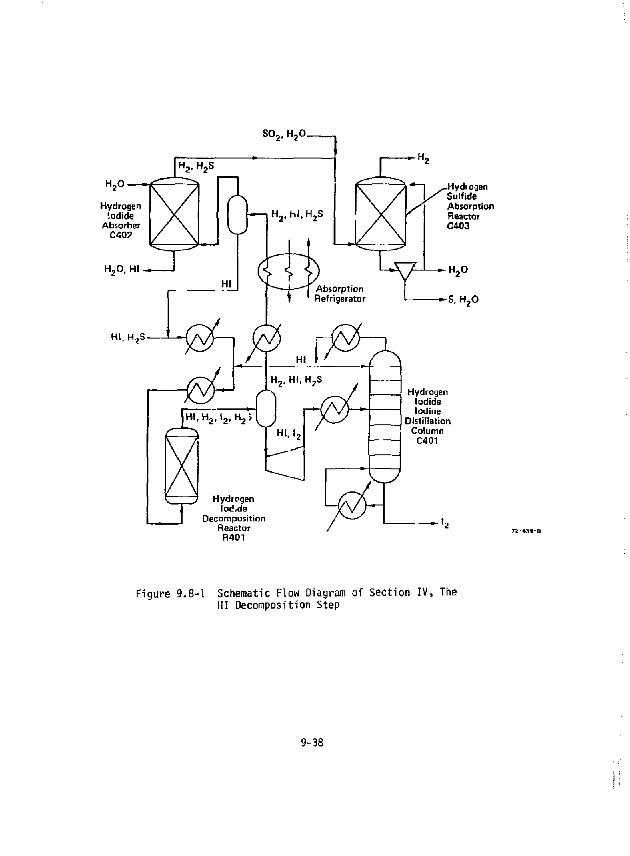
•"""] ^-Hydicgen Sulfide Absorption Reactor C403

H I , H , S -

\ y Hydrogen lod.de

Decomposition Reactor R401

Hydrogen Iodide Iodine

Distillation Column

C401

Figure 9.8-1 Schematic Flow Diagram of Section IV, The HI Decomposition Step

9-38

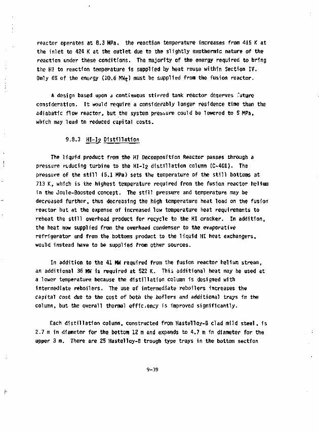
reactor operates at 8.3 MPa. the reaction temperature increases from 415 K at the inlet to 424 K at the outlet due to the slightly exothermic nature of the reaction under these conditions. The majority of the energy required to bring the HI to reaction temperature is supplied by heat reuse within Section IV. Only 6% of the energy (10.6 MWt) must be supplied from the fusion reactor.

A design based upon a continuous stirred tank reactor deserves future consideration. It would require a considerably longer residence time than the adiabatic flow reactor, but the system pressure could be lowered to 5 MPa, which may lead to reduced capital costs.

9.8.3 HI-Ig Pi stillation

The liquid product from the HI Decomposition Reactor passes through a pressure reducing turbine to the HI-I2 distillation column (C-401). The pressure of the still (5,1 MPa) sets the temperature of the s t m bottoms at 713 K, which is the highest temperature required from the fusion reactor helium in the Joule-Boosted concept. The still pressure and temperature may be decreased further, thus decreasing the high temperature heat load on the fusion reactor but at the expense of increased low temperature heat requirements to reheat the still overhead product for recycle to the HI cracker. In addition, the heat now supplied from the overhead condenser to the evaporative refrigerator and from the bottoms product to the liquid HI heat exchangers, would instead have to be supplied from other sources.

In addition to the 41 MW required from the fusion reactor helium stream, an additional 36 HW is required at 522 K. This additional heat may be used at a lower temperature because the distillation column is designed with intermediate reboilers. The use of intermediate reboilers increases the capital cost due to the cost of both the boilers and additional trays in the column, but the overall thermal effic.ency is Improved significantly.

Each distillation column, constructed from Hastelloy-B clad mild steel, is 2.7 m in diameter for the bottom 12 m and expands to 4.7 m in diameter for the upper 3 m. There are 25 Hastelloy-B trough type trays in the bottom section

9-39

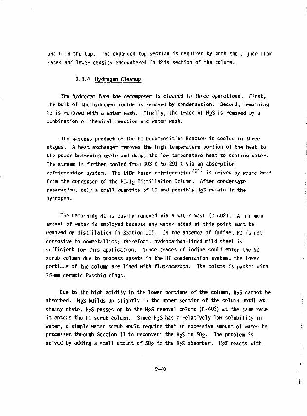
and 6 in the top. The expanded top section is required by both the higher flow rates and lower density encountered in this section of the column,

9.8.4 Hydrogen Cleanup

The hydrogen from the decomposer is cleaned in three operations. First, the bulk of the hydrogen iodide is removed by condensation. Second, remaining lii is removed with a water wash. Finally, the trace of H2S is removed by a combination of chemical reaction and water wash.

The gaseous product of the HI Decomposition Reactor is cooled in three stages. A heat exchanger removes the high temperature portion of the heat to the power bottoming cycle and dumps the low temperature heat to cooling water. The stream is further cooled from 303 X to 291 K via an absorption refrigeration system. The LiBr based refrigeration*2!' is driven by waste heat from the condenser of the HI-I2 Distillation Column. After condensate separation, only a small quantity of HI and possibly H2S remain in the hydrogen.

The remaining HI is easily removed via a water wash (C-402), A minimum amount of water is employed because any water added at this point must be removed by distillation in Section III. In the absence of iodine, HI is not corrosive to nonmetallics; therefore, hydrocarbon-lined mild steel is sufficient for this application. Since traces of iodine could enter the HI scrub column due to process upsets in the HI condensation system, the lower porti^,,s of the column are lined with fluorocarbon. The column is packed with ?5-mm ceramic Raschig rings.

Due to the high acidity in the lower portions of the column, H2S cannot be absorbed, H2S builds up slightly in the upper section of the column until at steady state, H2S passes on to the H2S removal column (C-403) at the same rate it enters the HI scrub column. Since H2S has ? relatively low solubility in water, a simple water scrub would require that an excessive amount of water be processed through Section II to reconvert the H2S to SO2. The problem is solved by adding a small amount of SO2 to the H2S absorber, H2S reacts with

9-40

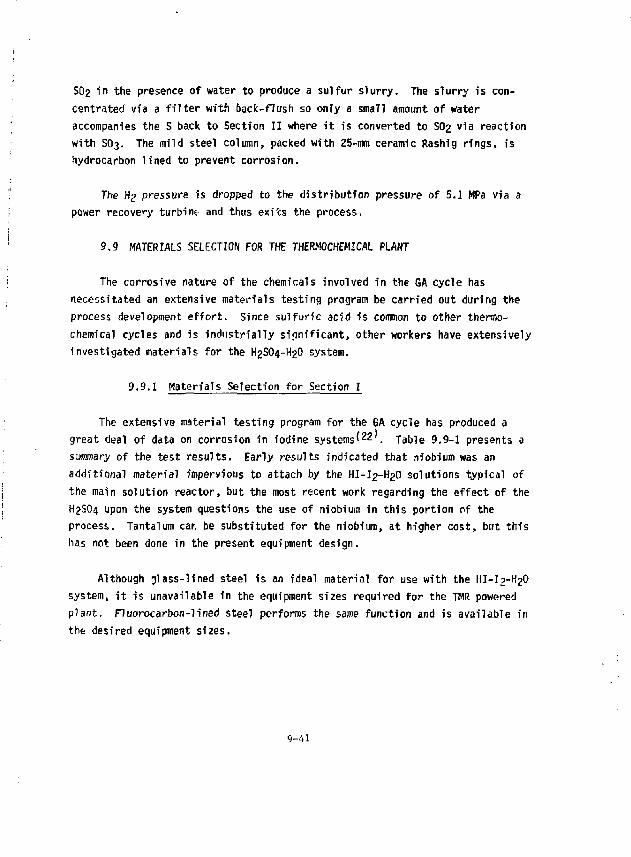
S02 in the presence of water to produce a sulfur slurry. The slurry is con­centrated via a filter with back-flush so only a small amount of water accompanies the S back to Section II where it is converted to SO2 via reaction with SO3. The mild steel column, packed with 25-mm ceramic Rashig rings, is hydrocarbon lined to prevent corrosion.

The H2 pressure is dropped to the distribution pressure of 5.1 MPa via a power recovery turbint and thus exits the process.

9.9 MATERIALS SELECTION FOR THE THERMOCHEMICAL PLANT

The corrosive nature of the chemicals involved in the GA cycle has necessitated an extensive materials testing program be carried out during the process development effort. Since sulfuric acid is common to other thermo-chemical cycles and is industrially significant, other workers have extensively investigated materials for the H2SO4-H2O system.

9.9.1 Materials Selection for Section I

The extensive material testing program for the GA cycle has produced a great deal of data on corrosion in iodine systemsf 2 2'. Table 9.9-1 presents a summary of the test results. Early results indicated that niobium was an additional material impervious to attach by the HI-I2-H2O solutions typical of the main solution reactor, but the most recent work regarding the effect of the H2SO4 upon the system questions the use of niobium in this portion of the process. Tantalum car. be substituted for the niobium, at higher cost, but this has not been done in the present equipment design.

Although glass-lined steel is an ideal material for use with the HI-I5-H2O system, it is unavailable in the equipment sizes required for the THR powered plant. Fluorocarbon-lined steel performs the same function and is available in the desired equipment sizes.

9-41

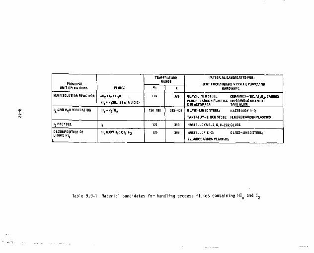
PRINCIPAL UNIT-OPERATIONS FLUIDS

TEMPERATURE RANGE

MATERIAL CANDIDATES FOR:

HEAT EXCHANGERS. VESSELS. PUMPS AND HARDWARE

PRINCIPAL UNIT-OPERATIONS FLUIDS aC K

MATERIAL CANDIDATES FOR:

HEAT EXCHANGERS. VESSELS. PUMPS AND HARDWARE

MAIN SOLUTION REACTION S0 2 * l2 + H 2 O — -

HI,tH 2 S0 4 l55W!4ACIDI

12S 398 GLASS-LINED STEEL; CERAMICS - SIC, A1 2 0 3 , CARBON FLUOROCARBON PLASTICS IMPERVIOUS GRAPHITE & ELASTOMERS: TANTALUM

l 2 ANDH 2 0 SEPARATION H l x *H jP0 4 120-150 393-431 GLASS-LINED STEEL: HASTELLOV B-2;

TANTALIIM-IINED STEEL: FLUOROCAREON PLASTICS

l 2 RECYCLE <2 120 393 HASTELLOVS B-2. G. C-276: GLASS

DECOMPOSITION OF Liauin ui x

HI„U0WH 2 0) ; l 2 ;H 2 IZO 393 HASTELLOV B-2; GLASS-LINEDSTEEL;

FLUOROCARBON PLASTICS;

Table 9.9-1 Material candidates for handling process fluids containing HI x and I.

9.9.2 Materials Selections for Section I I

Materials selections need to be made for the following process units for Section I I :

o Hulti-Effect Evaporator o H2SO4 Boiler 0 Joule-Boosted Decomposer 0 Fluidized Bed Decomposer 0 Decomposer Recuperator 0 Decomposer Cooler

Table 9.9-2 presents a summary of the material investigations by GA' 2 2 for the sulfuric acid sections of the process.

Hulti-Effect Evaporator and HpSOa Boiler

Materials problems are similar for the Multi-Effect Evaporator and the H2SO4 Boiler. The main problem Is to provide a heat exchanger that is tolerant of hot concentrated sulfuric acid. All known metallic heat exchanger materials (except for expensive noble metals such as Au and Pt), ire severely corroded by these H2SO4 solutions above temperatures of A.500 K. A number of ceramic and Intermetallic materials have been tested in hot concentrated H2SO4 at 633-693 K in recent years at LLNL^23»24' a n < | a t Westinghouse'^SJ. The top candidate materials from both corrosion resistance and heat exchanger design standpoints are the following:

0 Siliconized SiC 0 "CrSi2" coated Incoloy-800 0 Durichlor-51 (Fe-14S S1-4S Cr)

All of these materials depend upon the development of a corrosion resistant Si02 scale on the surface to provide protection against corrosion by H2SO4. Similarly, I t is well known that pure s i l ica glass (S102'» s u c n a s 1 n t n e f o r m

of si l ica brfck, is inert to corrosion by H2SO4.

9-43

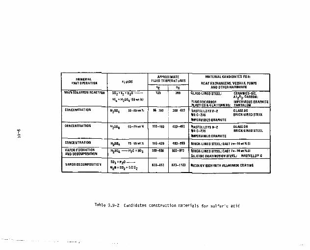
PRINCIPAL UNIT OPERATION FLUIDS

APPROXIMATE FLUID TEMPERATURES

MATERIAL CANDIDATES FOR:

HEAT EXCHANGERS. VESSELS. PUMPS AND OTHER HARDWARE

PRINCIPAL UNIT OPERATION FLUIDS

°C "K

MATERIAL CANDIDATES FOR:

HEAT EXCHANGERS. VESSELS. PUMPS AND OTHER HARDWARE

MMN SOLUTION REACTION S0 2

+ >2 + H2D

Hl x *H 2 S0 4 [55ivtHI

125 398 tLASSLINED STEEL: CERAMICS-SiC. A1 2 0 3 . CARBON:

tLUORQCARBOM IMPERVIOUS GRAPHITE JLASTICS& ELASTOMERS; TANTALUM

CONCENTRATION HjSO, 55-65wt!i 95 150 36B-423 llASTELLOVSD-2 GLASS OR OR C-276 BRICK-LINED STEEL IMPERVIOUS GRAPHITE

CONCENTRATION H2SO, 55-75 wt 54 1SO-180 423-453 HASTELLDYS B-Z GLASS OR OR C-276 BRICK-LINED STEEL IMPERVIOUS GRAPHITE

CONCENTRATION H2SO4 75-MwtH 110-420 453-693 IRICK-IIMED STEEL: CAST Fe-14wtXSI

VAPOR FORMATION AND DECOMPOSITION

H 2 S0 4 H jO*S0 3 330-600 603-873 4RICKUNED STEEL; CAST Fe-14wtXSi SUICIDE COATINGS ON STEEL: HASTELLOY G

VAPOR DECOMPOSITION SOj + H 20

Hzo + so 2 +if lo 2

G0O-85Q 873-1123 INCOLOY 800H WITH ALUMINIOE COATING

Table 9.9-2 Candidates construction materials for sulfuric acid

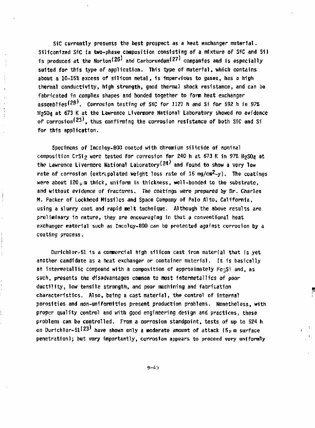
SiC currently presents the best prospect as a heat exchanger material. Siliconized SiC (a two-phase composition consisting of a mixture of SiC and Si) is produced at the Norton(26' and Carborundum'27 companies and is especially suited for this type of application. This type of material, which contains about a 10-15% excess of silicon metal, is impervious to gases, has a high thermal conductivity, high strength, good thermal shock resistance, and can be fabricated in complex shapes and bonded together to form heat exchanger assemblies* 2 8'. Corrosion testing of SiC for 1121 h and Si for 592 h in 97% H2SO4 at 673 K at the Lawrence Livermore National Laboratory showed no evidence of corrosion'23'( t h U S confirming the corrosion resistance of both SiC and Si for this application.

Specimens of Incoloy-800 coated with chromium silicide of nominal composition CrSi2 were tested for corrosion for 240 h at 673 K in 97% H2SO4 at the Lawrence Livernore National Laboratory(24' a n d found to show a very low rate of corrosion (extrapolated weight loss rate of 15 mg/cm^.y). The coatings were about 120ptn thick, uniform in thickness, well-bonded to the substrate, and without evidence of fractures. The coatings were prepared by Dr. Charles H. Packer of Lockheed Missiles and Space Company of Palo Alto, California, using a slurry coat and rapid melt technique. Although the above results are preliminary in nature, they are encouraging in that a conventional heat exchanger material such as Incoloy-800 can be protected against corrosion by a coating process.

Durlchlor-51 is a commercial high silicon cast iron material that is yet another candidate as a heat exchanger or container material. It is basically an intermetallic compound with a composition of approximately Fe^SI and, as such, presents the disadvantages common to most fntermetallics of poor ductility, low tensile strength, and poor machining and fabrication characteristics. Also, being a cast material, the control of internal porosities and non-uniformities present production problems. Nonetheless, with proper quality control and with good engineering design and practices, these problems can be controlled. From a corrosion standpoint, tests of up to 524 h on Durichlor-5lf23' n a v e shown only a moderate amount of attack (5ym surface penetration); but very importantly, corrosion appears to proceed very uniformly

9-45

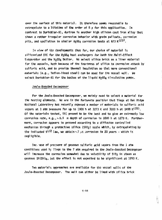
over the surface of this material. It therefore seems reasonable to extrapolate to a lifetime of the order of 5 y for this application. In contrast to Dur1chlor-5l, duriron is another high silicon cast iron alloy that shows a rather irregular corrosion behavior with grain pullouts, corrosion pits, and spallation in similar H2SO4 corrosion tests at 673 K^ 2 3'.

In view of t}ve developments thus far, our choice of material is siliconized SiC for the H2SO4 heat exchangers for both the Multi-Effect Evaporator and the H2SO4 Boiler. We select silica brick as a liner material for the vessels, both because of the inertness of silica to corrosive attack by sulfuric acid, and to provide thermal insulation so that more conventional materials (e.g., Teflon-lined steel) can be used for the vessel wall. We select Durichlor-51 for the bodies of the liquid H2SO4 circulation pumps.

Joule-Boosted Decomposer

For the Joule-Boosted Decomposer, we mainly need to select a material for the heating elements. We are in the fortunate position that Tiegs at Oak Bidge National Laboratory has recently exposed a number cf materials to sulfuric acid vapors at 1 atm pressure for up to 1900 h at 1273 K and 3300 h at 1498 K< 2 8'. Of the materials tested, SiC proved to be the best and to give an extremely low corrosion rate, e.g.,-^0.5 m depth of corrosion in 1000 h at 1273 K. Further­more, corrosion appears to proceed according to a diffusion controlled mechanism through a protective silica (Si02) scale which, by extrapolating by the indicated t 1/ 2 law, we obtain 7 vrr, corrosion in 20 years - which is negligible.

Inc. 'ase of pressure of gaseous sulfuric acid vapors from the 1 atm conditions used by Tiegs to the 7 atm required in the Joule-Boosted Decomposer will increase the corrosion somewhat due to volatility of SIO2 in steam as gaseous S K O H H , but the effect is not expected to be significant at 1250 K.

Two materials approaches are available for the vessel walls of the Joule-Boosted Decomposer. The wall can either be lined with silica brick

9-46

backad by 316 stainless steel maintained abcve the condensation temperature of sulfuric acid ( 680 K), or i t can be constructed of Incoloy-800H which is limited to a maximum temperature of 050 K because of creep strength limitations (see further details on Incoloy-800H properties in the discussior. of the Fluidized Bed Decomposer below). Selection of the materials approach to use wi l l depend upon engineering considerations.

Fluidized Bed Decomposer

The main materials problem in the Fluidized Bed Decomposer is selection of a heat exchanger material to meet corrosion resistance and creep strength requirements.

Corrosion tests on a number of heat exchanger alloys for H2SO4 vapor decomposers have been carried out at JRC Ispra and at the General Atomic company at temperatures in the 773-1173 K range. Their r e s u l t s ' ^ indicate that as bare uncoated alloys, Incoloy-800H and Inconel-625 provide the best materials with anticipated lifetimes of a few years. A substantial gain in l i fet ime can be achieved by using an aluminide-coated Incoloy-800H on the surface exposed to the decomposing SO3 gas. This gives an unusually stable coating-substrate combination that stabilizes in coating thickness and weight change after an exposure of 200-300 hours to the gaseous H2SO4 products* 2 5 . Corrosion protection is apparently afforded by an AI2O3 f i lm , and imperfections in the coating are self-healing. The useful l i f e of alumini de-coated Incoloy-800H for this application is believed to be of the order of 20 years. On the high pressure helium side, corrosion is not a problem.

From a consideration of creep strength, cost, and fabrication issues, Inconel-617, Inconel-625, and Incoloy-800 (or Incoloy-800H) appear to provide the best alternatives. Stress rupture and creep properties for Inconel-625 and Incoloy-800 are comparable^'. Although creep strength data are not available for Inconel-617, i t shows 1000-hour stress rupture strengths that are three times higher(30) than for the other two alloys. Thus, extrapolations of the available data for Inconel-625 and Incoloy-800 suggest a tensile creep strength for 1% creep in 100,000 hours of 2000 ± 50% psi (1.4 x 10? Pa) at 1100 K and

9-47

1200 + 30% psi (8.2 x 10$ Pa) at 1150 K. We estimate the corresponding values for Inconel-617 to be 6000 + SOS psi {4.1 x 107 Pa) at 1100 K and 3600 + 30$ psi (2.4 x 10? Pa) at 1150 K based on the argument that the creep strengths scale as a fraction of the long-term creep rupture data similar to Inconel-625 and Incoloy-800. Although no creep data are available for Ir>co1oy-800H, i t is a material that has been designed for higher strength than lncoloy-800 and should give a better performance.

From a consideration of both corrosion and creep strength we select rnco!oy-800H as tiie heat exchanger material for the Fluidized Bed Decomposer. A minimum wall thickness 3 mm is required to maintain material integrity after allowances for-v 0.5 mm corrosion penetration. An aluminide protective coating is recommended on the SO3 side of the heat exchanger to obtain a longer equip­ment l i f e .

Selection of a vessel material for the Fluidized Bed Decomposer involves the same considerations as for the Ooule-Boosted Decomposer. Either a si l ica brick-lined 316 stainless steel vessel or an Inco1oy-800H vessel would be suitable.

Decomposer Recuperator

The wain materials problem for the Decomposer Recuperator is for the Heat Exchanger, and as was the case for the Fluidized Bed Decomposer, corrosion and long-term creep strength are the main considerations. Temperatures are suf­f ic ient ly lower here (i<1050 K) that the problems are less severe. Therefore, an aluminide coating should not be needed. We select Incoloy-800H at a wall thickness of 3 ran as the preferred material with Inconel-617 as a backup for the Decomposer Recuperator heat exchanger. Selections for the vessel walls are either si l ica brick-lined 316 stainless steel or Incoloy-SOOH.

Decomposer Cooler

Transport piping from the Decomposer Recuperator to the Decomposer Cooler would be made from Incoloy 800H. The Decomposer Cooler heat exchanger is an

9-48

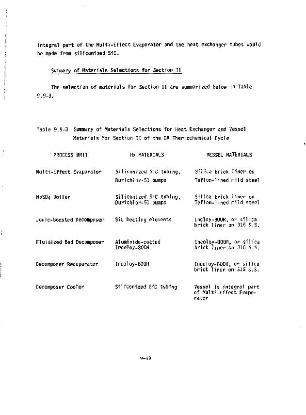
in tegra l part of the Mu l t i -E f fec t Evaporator and the heat exchanger tubes would

be made from s i l i con ized SiC.

Summary of Materials Selections fo r Section H

The select ion of materials for Section I I are summarized below in Table

9.9-3.

Table 9.9-3 Summary of Materials Selections for Heat Exchanger and Vessel

Mater ia ls for Section 11 of the GA Thermochemical Cycle

PROCESS UNIT Hx MATERIALS VESSEL MATERIALS

MuTt i-Effect Evaporator

H2SO4 Boi ler

Joule-Boosted Decomposer

Flu id ized Bed Decomposer

Decomposer Recuperator

Decomposer Cooler

S i l i con ized SiC tub ing , DurichV)r-51 pumps

Si l icon ized SiC tub ing , Dur ichlor-51 pumps

SiL heating elements

Alumini de-coated Incoloy-800H

Incoloy-80QH

Si l iconized SiC tubing

S i l i ca br ick l i n e r on Tef lon- l ined mi ld steel

S i l i ca br ick l i n e r on Tef lon- l ined mi ld steel

Incloy-800H, or s i l i c a br ick l i n e r on 316 S.S.

Incoloy-800H, or s i l i c a br ick l i n e r on 316 S.S.

Incoloy-800H, or s i l i c a br ick l i n e r on 316 S.S.

Vessel i s in tegra l part of Mu l t i -E f fec t Evapo­ra tor

9-49

9.9.3 Material Selection for Sections H I and IV

Material selection for Sections III and IV is similar to that selected for Sections I and II. The information in Table 9.9-1 is applicable to the iodine-HI regions of Sections H I and IV. Phosphoric acid adds no new complexity except in the high temperature portions of the process, acid brick is necessary as a thermal protection for teflon liners. In addition, Hastelloy C has been recommendedl^l) for use with boiling concentrated phosphoric acid.

9.10 SAFETY CONSIDERATIONS

The main safety issues involve the control, handling, and containment of tritium, liquid lithium, and sulfuric acid. The safety issues regarding tritium and liquid lithium were reviewed and discussed in some detail in the 1980 report^ 9), and it was concluded that adequate controls were designed into the system to maintain proper safety. We have applied similar consideratoins in the current designs, including particular attention to both residual and accidental leakages of tritium into the environment or product, tritium inventories 1n the system, and potential problems of liquid lithium fires. We feel that the safety issues have been welT met, and many of the details have been covered in this year's text. We refer the reader to last year's report for further details.

In regard to safety of sulfuric acid, it is important that conservative designs be maintained on the vessels and piping containing hot liquid and gaseous sulfuric acid and its decomposition products, since sulfuric acid introduced into the environment is a serious health hazard. He feel that we have taken adquate measures in our design stuuicS, snd recognize further that the sulfuric acid industry has been a large and well-established m o u s e y ami one that we can draw on for future design Information as needed for assuring a safe plant.

9-50

9.U. PLANT LAYOUT AND PLOT PLAN

9.11.1 Plant Layout

A complete plant process layout, assembling all of the sections, was prepared for last year's eport^) and is given earlier in the report in Figure 9.0-1, complete with important process parameters and labels on key process sections and on process units. The legend describes the symbolic representation used. Generally we have attempted to arrange the highest tem­perature processes at the top of the figure and the lower temperature processes at the bottom. At the immediate left is the Tandem Mirror Fusion driver and the associated helium coolant streams operating turbo-generators and process heat exchangers as a topping cycle and bottoming into a steam-r<ankine cycle for additional electricity generation.

A larger version of this complete process flow diagram and flowsheet are available upon request. However, this reduced-size figure has been included to help one grasp the overall picture of the Fuslon/Synfuels Process concept.

This year's version of the flowsheet has ;iot been integrated into a similar one full layout but simplified flowsheets for each section have been presented in the text of this section. Last year's composite flowsheet still serves the purpose of presenting the scale of the total thermochemical process.

9.11.2 Plot Plan

An artist's conceptual drawing of the plot plan as given in last year's report'!) is shown in Figure 9.11-1. Changes in this year's design did not materially affect space requirements so this plot plan still gives a rough idea of the approximate land area and relative sizes of the TMR nuclear island, turbine-generator, steam generator and process heat exchanger building, as well as the rest of the chemical plant. We conclude from the plot plan that this plant is quite compact, and raises no new Issues regarding heat transport distances, safety, etc.

9-51

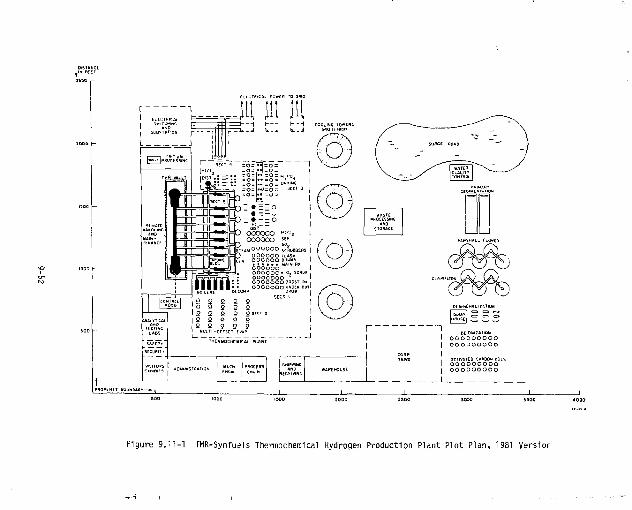
t PROPERTY

Figure 9,11-1 TMR-Sjnfuels Thermochemical Hydrogen Production Plant Plot Plan, 1981 Version

References for Section 9.0

1. R. W. Werner, et aJ., "Conceptual Design Study FY 1981, Synfuels front Fusion using the Tandem Mirror Reactor and a Thermocheroica") Cycle to Produce Hydrogen," Lawrence Livermore National Laboratory, Report UCID-19311, February 9, 1982.

2. J. I1. Norman, G. E. Besenbruch, L. C. Brown, 0. R. O'Keefe, and C. L. Mian, "Thermochemical Water-Splitting Cycle, Bench-Scale Investigations and Process Engineering, Final Report for the Period Ending February 1977 through December 31, 1981," DOE Report DOE/ET/26225-1, General Atomic Company Report GA-A16713, May 1982.

3. G. £. Besenbruch, K. H. McCorkle, J. H. Norman, D. R. O'Keefe, J. R. Schuster, and K. Yoshitnoto, "Hydrogen Production by tne GA Sulfur-Iodine Process, A Progress Report," Hydrogen Energy Progress, Proceedings of the 3rd World Hydrogen Energy Conference, Tokyo, Japan, 23-26 June 1980, Vol. 1 edited by T. N. Veziroglu, K. Fueki and T. Ohta, Pergamon Press, Oxford, 1980, p. 243.

4. J. H. Norman, G- E. Besenbruch, and L. C. Brown, "Solar Production of Hydrogen using the Sulfur-Iodine Thermochemical Water Splitting Cycle, Final Report," General Atomic Company Report GA-C-16493.

5. J. H. Norman, "Studies of the Sulfur-Iodine Thermochemical Water-Splitting Cycle," Hydrogen Energy Progress, Proceedings of »:» 3rd World Hydrogen Energy Conference, Tokyo, Japan, 23-26 June 1980, Vol. 1, edited by T. N. Veziroglu, K. Fueki, and T. Ohta, Pergamon Press, Oxford, 1980, p. 277.

6. 0. R. O'Keefe and 0. H. Norman, "The Liquid Hydrogen Iodide Decomposition Process Step for Water-Splitting Applications," Hydrogen Energy Progress, Proceedings of the 3rd World Hydrogen Energy Conference, Tokyo, Japan, 23-26 June l^SO, Vol. 1, edited by T. N. Veziroglu, K. Fueki, and T. Ohta, Pergamon Press, Oxford, 1980, p. 277.

9-53

7. F. F. Rupert, "A Study of the System Hydrogen Chloride and Water," J. Am. Chem. Soc. 31, 851 (1909).

8. "Thermochemical Water-Splitting Cycle, Bench-Scale Investigations and Process Engineering, Annual Report for the Period February through December 31, 1977," General Atomic Company Report, GA-14950, April 1978.

9. L. N. Horsley, "Azeotropic Data III," Advances in Chemistry Series, Vol. 116, American Chemical Society, Washington, D.C., 1973.

10. D. fl. O'Keefe and J. H. Norman, "The Liquid Hydrogen Iodide Decomposition Process Step for Watc-Splitting Applications," Hydrogen Energy Progress, Proceedings of the 3rd World Hydrogen Energy Conference, Tokyo, Japan, 23-26 June 1980, Vol. 1, edited by T. N. Veziroglu, K. Fueki, and T. Ohta, Pergamon Press, Oxford, 1980, p. 277.

11. A. F. Ryabinina and V. A. Oshman, "Thermal Decomposition of Aqueous Sulfur Dioxide Solutions," Tr. Ural, lesotekh, Inst. l'J72, No. 28, 182 (Russ), Chem. Abstracts 79, 58115p, 1973.

12. "JANAF Thermochemical Tables," Dow Chemical Company, Midland, Michigan, September 30, 1977.

13. F. w. Giaugue, et al., "Thennodyr^niic Properties of Aqueous Sulfuric Acid Solutions and Hydrales from 15 to 300K," J. Am. Chem. Soc. 82, 62 (1960).

14. "Thermochemical Water-Splitting Cycle, Bench-Scale Investigations and Process Engineering Annual Report for the Period October 1, 1978 through September 30, 1979," DOE Report GA-A15788, General Atomic Company, March 1980.

15. H. Coombs, et al., "High-Temperature Ceramic Heat Exchanger, Final Report, July 1979," AiResearch Manufacturing Company of California, Torrance, CA, Report FP-1127, Research Project 545-1, report prepared for Electric Power Research Institute, Palo Alto, CA. R. H. Richman, EPRI Project Mgr., 1979.

9-54

16. R. H. Perry and C. W. Chilton, editors, "Chemical Engineers' Handbook," 5th edition, McGraw-Hill, New York, 1973, p. 10-21.

17. "Gem!ins Handbuch der Anorganischen Cftemie, Schwefel, System Number 9," Velag Chemle, GMbH, Weinheim/Bergstrasse, West Germany, 1960, p. 662.

18. E.R.G. Eckert and R. H. Drake, "Analysis of Heat and Mass Transfer," McGraw-Hill, New York, 1972, p. 562.

19. R. W. Werner, et al., "Synfuels From Fusion - Producing Hydrogen With The Tandem Mirror Reactor and Theinocheinical Cycles," Lawrence Livermore National Laboratory, Report UCID-18909, Vol. ! and II, January 21, 1981.

20. "HT?R Tfcsnnochemical Water-Splittiri for Hydrogen Production, Annual Report for the Period January 1, 197S through December 31, 1975," General Atomic Company Report GA-A13800, January 31, 1976.

21. F. J. Evans, Jr., "Equipment Design Handbook for Refinery and Chemical Plants," second edition, Vol. 1, Gulf Publishing Co., Houston, TX, 1979, pp. 184-191.

22. P. W. Trester and H. G. Staley, "Assessment and Investigation of Containment Materials for the Sulfur-Iodine Thermochemical Water-Splitting Process for Hydrogen Production, Final Report (July 1979-CsCemoer 1980)," Gas Research Institute Report, GRI-80/0081, May 19f!l.

23. 0. H. Krikorian, "Material Corrosion Studies for a Sulfuric Acid Vaporizer," Lawrence Livermore National Laboratory Report UCRL-81856, October 27, 1978.

24. 0. H. Krikorian, "Corrosion Testing of Materials in Hot Concentrated Sulfuric Acid," Lawrence Livermore National Laboratory Report UCRL-83411, September 27, 1979.

9-55

25. R. L. Amnion, G. Yatsko, A. Irwin, and G. H. Furbman, "Materials Consideration for the Westinghouse Sulfur Cycle Hydrogen Production Process," unpublished paper presented at the Second World Hydrogen Energy Conference, Zurich, Switzerland, 21-24 August 1978.

?.S. M. L. Torti, J. W. Lucek, and G. Q. Weaver, "Densified silicon Carbide -An Interesting Material for Diesel Applications," Technical paper Series 780071, Society of Automotive Engineers Congress and Exposition, Detroit, February 27 through March 3, 1978. See also brochures of the Norton Company, Worchester, Massachusetts on "Noralide Advanced Ceramics," and "Ceramics for Energy."

27. Edwin Craft, Carborundum Company, Niagara Falls, New York, private communication regarding bending of KT-Silicon carbide to form U-tubes, October 1979.

26. T. N. Tiegs, "Materials Testing for Solar Thermal Chemical Process Heat," Oak Ridge National Laboratory, Oak Ridge, TN, Report ORNL/TM-7833, October 1991.

29. 0. H. Krikorian, "Materials Problems in Production, Transport and Storage of Hydrogen,' •""vermore National Laboratory Report, UCRL-83771, January 2, 1980.

30. Engineering Alloys Digest, Inc., Upper Montclair, Mew Jersey: Filing code Ni-179, Inconel alloy 617, September 1972; Filing code Ni-121, Inconel alloy 625, February 1967; and Filing code 55-136, Incoloy alloy 800, September 1972.

31. J. H. Perry, editor, "Chemical Engineers' Handbook," 3rd edition, McGraw Hill, New York, 1950, p. 1507.

9-56

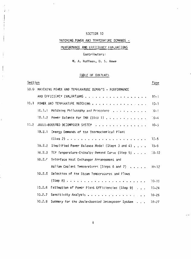
I

SECTION 10 MATCHING POWER AND TEMPERATURE DEMANDS -PERFORMANCE AND EFFICIENCY EVALUATIONS

Contributors: M. A. Hoffman, D. S. Rowe

TABLE OF CONTENTS Section Page 10.0 MATCHING POWER AND TEMPERATURE DEMANDS - PERFORMANCE

AND EFFICIENCY EVALUATIONS 10-1 10.1 POWER AND TEMPERATURE MATCHING 10-1

10.1.1 Matching Philosophy and Procedure . . . 10-1 10.1.2 Power Balance for TMR (Step 1) 10-4

10.2 JOULE-BOOSTED DECOMPOSER SYSTEM 10-5 10.2.1 Energy Demands of the Thermochemical Plant

(Step 2) 10-5 10.2.2 Simplified Power Balance Model (Steps 3 and A) . . . . 10-9 10.2.3 TCP Temperature-Enthalpy Demand Curve (Step 5) . . . . 10-12 10.2.'' Interface Heat Exchanger Arrangement and

Helium Coolant Temperatures (Steps 6 and 7) 10-12 10.2.5 Selection of the Steam Temperatures and Flows

(Step 8) 10-19 10.2.6 Estimation of Power plant Efficiencies (Step 9) , . . 10-24 10.2.7 Sensitivity Analysis 10-26 10.2.8 Summary for the Joule-Boosted Decomposer System . . . 10-27

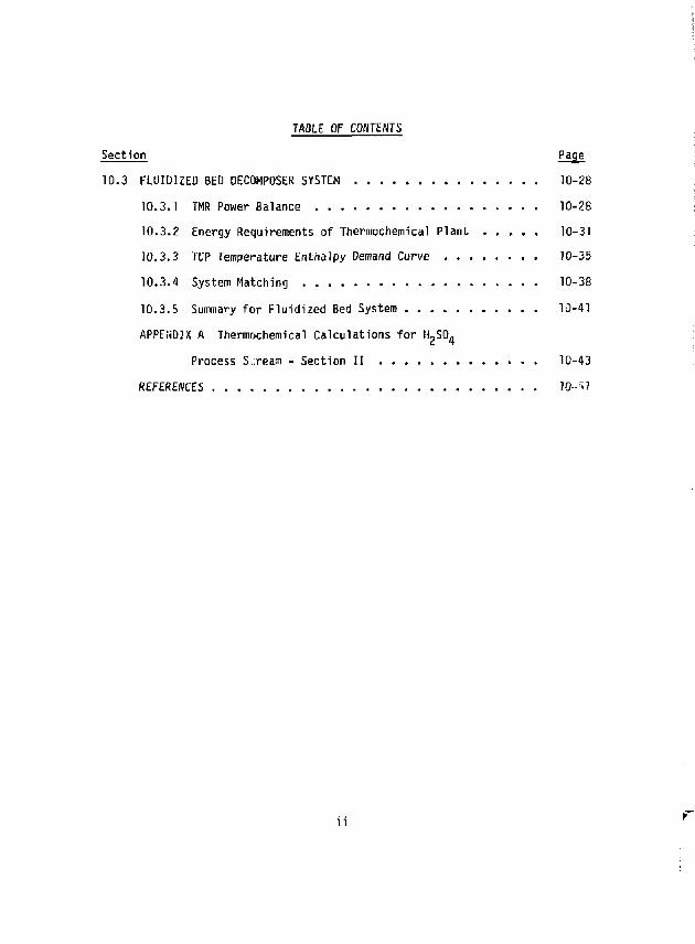
TABLE OF CONTENTS

Section £ii££ 10.3 FLUIDIZED BED DECOMPOSER SYSTEM 10-28

10.3.1 TMR Power Balance 10-28 10.3.2 Energy Requirements of Thermochemical Plant 10-31 10.3.3 TCP Temperature Enthalpy Demand Curve . . . . . . . . 10-35 10.3.4 System Matching 10-38 10.3.5 Summary for Fluidized Bed System 10-41 APPENDIX A Thermochemical Calculations for H-SO^

Process S.ream - Section II 10-43 REFERENCES 70-^1

ii >

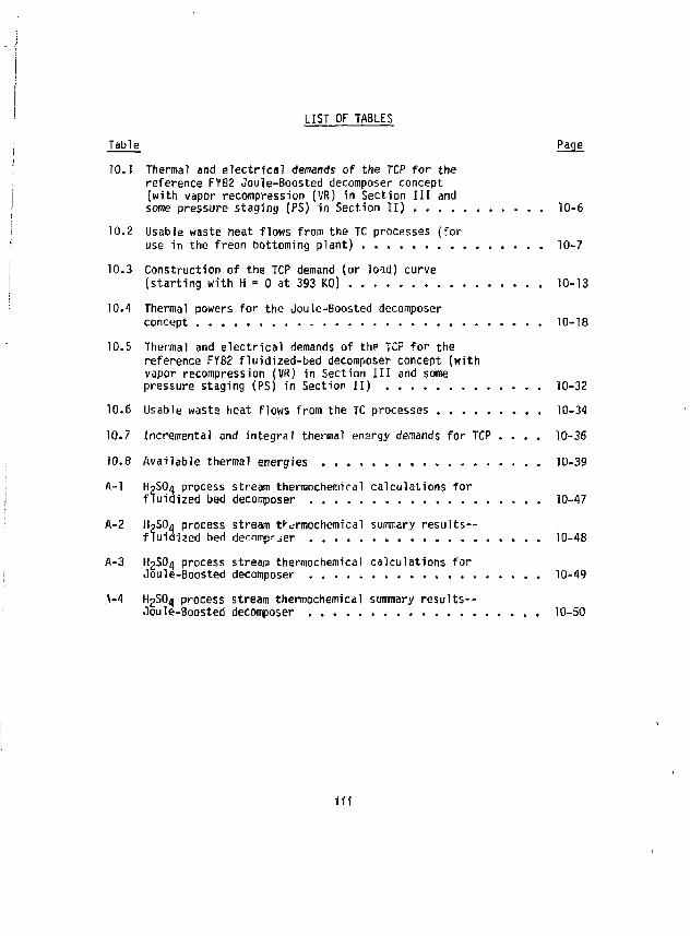
LIST OF TABLES Table Page TO.1 Thermal and electrical demands of the TCP for the

reference FY82 Joule-Boosted decomposer concept (with vapor recompression (VR) in Section III and some pressure staging (PS) in Section II) 10-6

10.2 Usable waste heat flows from the TC processes (for use in the freon bottoming plant) 10-7

10.3 Construction of the TCP demand (or load) curve (starting with H = 0 at 393 KO) 10-13

10.4 Thermal powers for the Joule-Boosted decomposer concept 10-18

10.5 Thermal and electrical demands of the TCP for the reference FY82 fluidized-bed decomposer concept (with vapor recompression (VR) in Section III and some pressure staging (PS) in Section II) 10-32

10.6 Usable waste heat flows from the TC processes 10-34 10.7 Incremental and integral thermal enargy demands for TCP . . . . 10-36 10.8 Available thermal energies . . . 10-39 A-1 HoSOa process stream thermocheriical calculations for

fluiaized bed decomposer 10-47 A-2 HoSO^ process stream t^rmochemical summary results—

fluiaized bed decomp-ier . 10-48 A-3 H2SO4 process stream thermochemicaI calculations for

Joule-Boosted decomposer 10-49 A-4 HgSO^ process stream thermochemical summary results--

Joule-Boosted decomposer 10-50

n'i

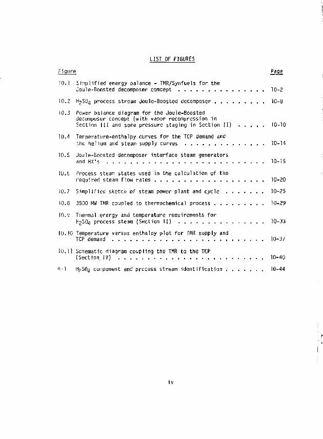
LIST OF FIGURES Figure Page 10.1 Simplified energy balance - TMR/Synfuels for the

Joule-Boosted decomposer concept 10-2 10.2 H2SO4 process stream Joule-Boosted decomposer 10-8 10.3 Power balance diagram for the Joule-Boosted

decomposer concept (with vapor recompression in Section III and some pressure staging in Section II) 10-10

10.4 Temperature-enthalpy curves for the TCP demand and the helium and steam supply curves 10-14

10.5 Joule-Boosted decomposer interface steam generators and HX's 10-15

10.6 Process steam states used in the calculation of the required steam flow rates 10-20

)0.7 Simplified sketch of steam power plant and cycle 10-25 10.8 3500 MW TMR coupled to thermochemical process 10-29 10.9 Thermal energy and temperature requirements for

H2SO4 process steam (Section II) 10-33 10.10 Temperature versus enthalpy plot for TMR supply and

TCP demand 10-37 10.11 Schematic diagram coupling the TMR to the TCP

(Section. IV) 10-40 A-'f H2SO4 component and process stream identification 10-44

IV

r

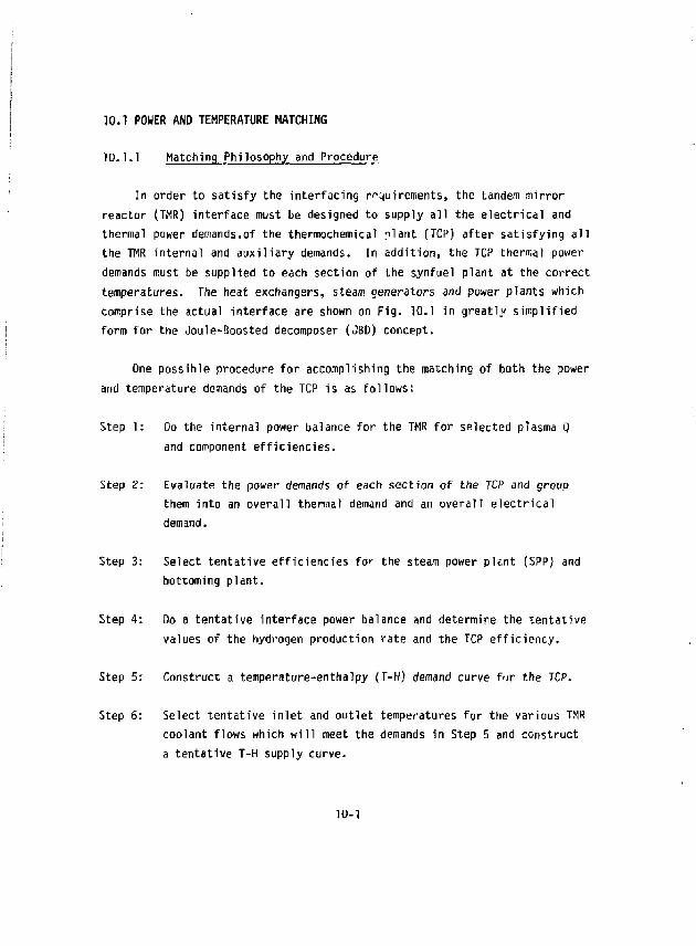
10.1 POWER AND TEMPERATURE HATCHING

10.1.1 Matching Philosophy and Procedure

In order to satisfy the interfacing requirements, the tandem mirror reactor (TMR) interface must be designed to supply all the electrical and thermal power demands.of the thermochemical plant (TCP) after satisfying all the TMR internal and auxiliary demands. In addition, the TCP thermal power demands must be supplied to each section of the synfuel plant at the correct temperatures. The heat exchangers, steam generators and power plants which comprise the actual interface are shown on Fig. 10.1 in greatly simplified form for the Joule-Boosted decomposer (JSD) concept.

One possible procedure for accomplishing the matching of both the power and temperature demands of the TCP is as follows:

Step 1: Do the internal power balance for the TMR for selected plasma Q and component efficiencies.

Step 2: Evaluate the power demands of each section of the TCP and group them into an overall thermal demand and an overall electrical demand.

Step 3: Select tentative efficiencies f c the steam power plant (SPP) and bottoming plant.

Step 4: Do a tentative interface power balance and determine the tentative values of the hydrogen production rate and the TCP efficiency.

Step 5: Construct a temperature-enthalpy (T-H) demand curve f-*r the TCP.

Step 6: Select tentative inlet and outlet temperatures for the various TMR coolant flows which will meet the demands in Step 5 and construct a tentative T-H supply curve.

10-1

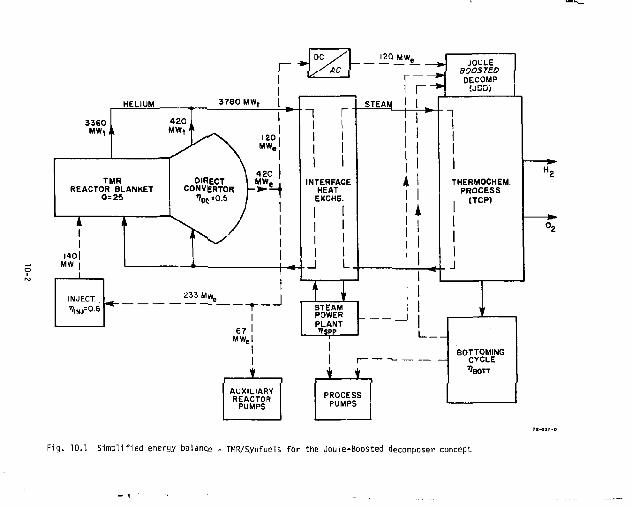
3360 MW, A

TMR REACTOR BLANKET

0=25

1401 MW

l i . i fO -6

L£_

1

INTERFACE HEAT

EXCHS.

I I I I

J L

STEAM POWER PLANT VSPP

O BOOST El r — * 1 DECOMF I I *1 USD)

STEAM

THERMOCHEM. PROCESS

i (TCP)

JL i_ PROCESS PUMPS

BOTTOMING CYCLE ' B O T T

F i g . 10.1 S i m p l i f i e d energy balance •• TMR/Synfuels f o r the Jouie-Boosted decomposer concept

Step 7: Draw a tentative interface arrangement showing the various inter­mediate heat exchangers required (steam generators in this study).

Step 8: By trial and error, determine the optimum steam flows and temperatures in each part of the interface so that the steam T-H curve fits in between the supply and demand curves.

Step 9: Estimate the actual efficiencies of the steam power plant and the bottoming plant based on the actual temperatures at which heat is available to them.

Step 10: If these efficiencies are very different than those assumed in Step 3, or if some power or temperature demand cannot be satisfied, redo the procedure starting at Step 3.

When the final results are reasonably self-consistent, then one possible solution to the interface matching has been found. However, it may not be the "optimum" solution, so that it may be necessary to try other heat exchanger arrangements to see if a better matching can be obtained.

For this FY82 study, we set as our primary objective to try to minimize the first wall, blanket and direct converter material temperature: required for the JBD concept; obtaining a high overall TCP efficiency was made a secondary objective. It is felt that the low materials temperatures will lead to a highly credible and cost effective design even with relatively low TCP efficiency, as discussed in Section 1,

The above ten-step procedure has been used in this conceptual design study to give reasonably rapid, approximate results for a wide variety of cases. In the following sections, the procedure will be illustrated in detail for the reference case selected for this FY82 Final Report.

10-3

10.1.2 Power Balance for the TMR (Step 1)

The power balance for a TMR (Step 1 above) for a plasma Q = 25 and a fusion power of 3500 MW is already indicated on Fig. 10.1. It can be seen that the first wall (FW), the blanket (BL) and the direct converters (DC) supply a total Of 3780 MW of thermal power to the TCP. In addition, the DC supplies a net electric power of 120 MW„ to the TCP.

This power balance is obtained as follows. The thermal power output from the TMR blanket and first wall is assumed to be equal to the neutron power times the blanket multiplication, M = 1.2:

Pt(BL + FW) = °' 8 Pfus * M = 3 3 6 ° M W t

About 8.SI of this power (285 Mw\ ) is deposited in the first-wall helium coolant, while the remainder (3075 MW.. ) is carried out by the blanket helium coolant.

The remaining 20% of the fusion power is assumed to eventually flow out the mirror exits to the direct converters as ion leakage (including the "halo" power) and be converted to electric power at an effective efficiency, n o c = 50%:

Pe(0C) = °' 2 0 * Pfus x "DC = 4 2 ° M W e

For a plasma Q = 25, the overall circulating power required to power the TMR (including neutral beam injection, RF heating, etc.) is:

e(CIRC) Q n I N J t

where rtiMi 's the overall average efficiency of all the injection devices, taken as 60%.

We assumed that roughly 67 MW would be required ;or auxiliaries such as vacuum pumps, helium refrigerators, etc. This leaves a net electric power

10-4

to the TCP of 120 MW e as shown on Fig. 10,1.

The total thermal power to the TCP consists of the 3360 MW. from the first wall and blanket plus 420 MW. rejected at high temperature rrci the direct converters. This sum is the 3780 MWfc shown in Fig. 10.1.

In Section 10.2, the power and temperature matching for the TCP employing the Joule-Boosted decomposer concept is described. Then in Section 10.3 the matching for the TCP employing the fluidi'zed bed decomposer concept is discussed.

10.2 JOULE-BOOSTED DECOMPOSER SYSTEM

10.2.1 Energy Oernands of the Thermochemical Plant (Step 2)

The overall TCP is divided into Sections 1, II, III, IV and V as described in Section 9 of this report. Section V of the TCP is the inter­face itself. Several different options for the TCP equipment and processes were investigated this year in an attempt to find the arrangement which appeared to be most cost effective, i.e., the lowest overall cost per mole of hydrogen produced.

The arrangement selected for the FY82 reference cas for the Joule-Boosted decomposer (JfiD) concspt retained vapor recompression (VR) in Section III and added pressure stagi j (PS) in Section II. The final energy retire­ments for each section assum* i in this FY82 study are summarized in Tables 10.1 and 10.2. (Some minor nanges in these values were made by GA after this table was prepared. Th • effect of these small changes will be treated by a sensitivity analysis in Section 10.2.7.) The very important H ?S0, process stream requirements are shown on Fig. 10.2. It can be seen from Table 10.1 that the TCP requires a total of 285 kJ of electric energy and 331 kJ t of thermal energy per mole of hydrogen produced.

The temperatures at which each thermal energy demand is required are

10-5

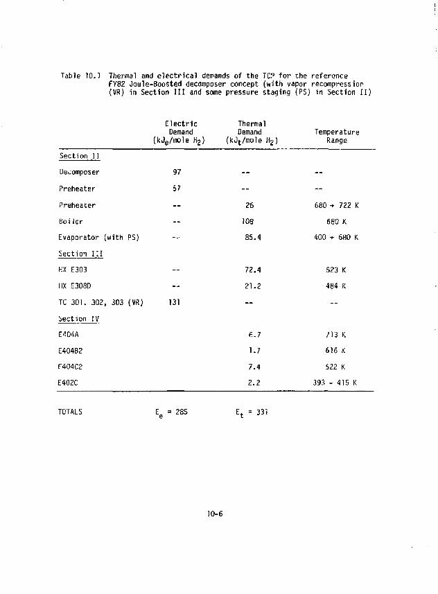
Table 10.1 Thermal and electrical demands of the TCP for the reference FY82 Joule-Boosted decomposer concept (with vapor recompression (VR) in Section III and some pressure staging (PS) in Section II)

Electric Demand

(kJe/mole Kj) Thermal Demand

(kJt/mole H 2) Temperature

Range Section II Decomposer 97 — — Preheater 57 — — Preheater — 26 680 ->• 722 K Boiler — 108 680 K Evaporator (with PS) — 85.4 400 + 680 K Section III HX E303 — 72.4 523 K HX E308D — 21.2 484 K TC 301, 302, 303 (VR) 131 — — Section IV E404A 6.7 713 K E404B2 1.7 616 K E404C2 7.4 522 K E402C 2.2 393 - 415 K

TOTALS e E t = 331

10-6

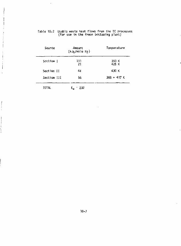
Table 10.2 Usable waste heat flows from the TC processes (for use in the freon bottoming plant)

Source Amount (kJt/mo'le H2)

Temperature

Section I 111 21

393 K 425 K

Section II 44 430 K Section III 56 368 * 417 K

TOTAL E w = 232

10-7

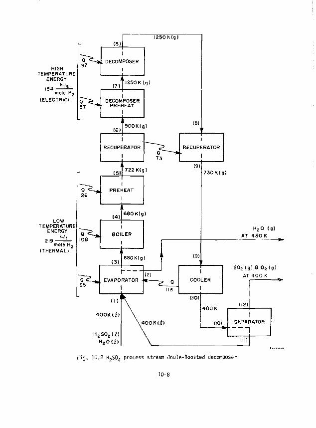
HIGH TEMPERATURE

ENERGY

154 V mole H 2

(ELECTRIC1

0 ' 97

LOW TEMPERATURE

ENERGY k J ,

219 — — — mole H 2

(THERMAL)

Q < 26

Q •= 108

l 2 5 0 K ( g ) (8)1

I

DECOMPOSER

I

i! (7)

I 250K (g)

DECOMPOSER PREHEAT

I t

(6) 900K(g)

722K(g)

I PREHEAT

I

(4) 680 K(g)

I BOILER

I i;

(3) 680K(g)

I EVAPORATOR

(8)

Q_

113

H 2 S 0 2 t i ) H z O ( i )

, 4 0 0 K ( i >

I

RECUPERATOR

I

19)

(9)

7 3 0 K ( g )

H 2 0 (g) AT 4 3 0 K

COOLER

110)

S 0 2 (g) a 0 2 ( g )

AT 4 0 0 K

4 0 0 K

(10)

0 2 ]

SEPARATOR

(II)

F i ^ . 10.2 H-SOjj process stream Jou le -Boos ted decomposer

10-8

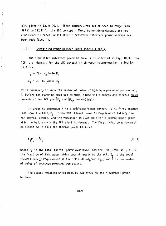
air J given in Table 10.1. These temperatures can be seen to range from 393 K to 722 K for the JBD concept. These temperature demands are not considered in detail until after a tentative interface power balance has been made (Step 4).

10.2.2 Simplified Power Balance Model (Steps 3 and 4)

The simplified interface power balance is illustrated in Fig, 1C3. The TCP total demands for the JBD concept (with vapor recompression in Section III) are:

e e 2 E t = 331 kJt/mole H 2

It is necessary to know the number of moles of hydrogen produced per second, N, before the power balance can be made, since the electric and thermal power demands of the TCP are NE p and NE t, respectively.

In order to determine H in a self-consistent manner, it is first assumed that some fraction, f., of the TMR thermal power is required to satisfy the TCP thermal demand, and the remainder is available for electric power gener­ation to help supply the TCP electric demand. The first relation which must be satisfied in thus the thermal power balance:

V t-fc t (10.1)

where P. is the total thermal power available from the TriR (3760 M W t ) , f, is the fraction of this power which goes directly to the TCP, E. is the total thermal energy requirement of the TCP (331 kOt/mcl Hj), and N is tne number of moles of hydrogen produced per second.

The second relation which must be satisfied is the electrical power balance:

10-9

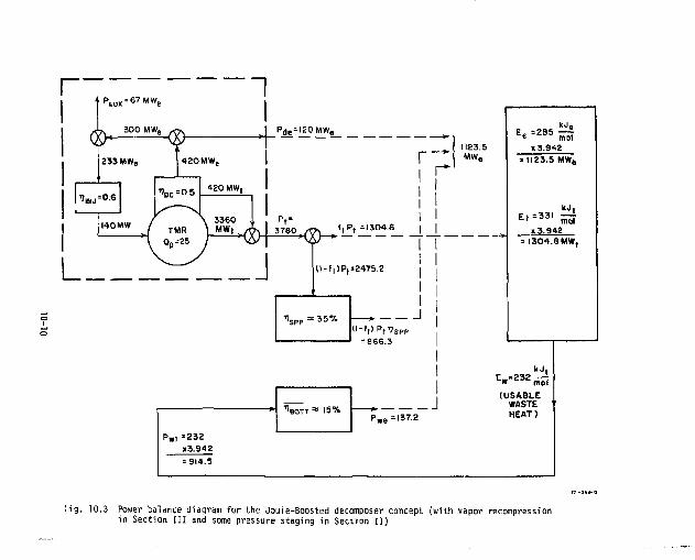
Mg. 10.3 Power balance diagram for the Joule-Boosted decomposer concept (with vapor recompression in Section I I I and some pressure staging in Section I I )

Pde^ 1 " V P t V P + EwNt\»OTT = N E e 00.2) where P. is the net electric power available to the TCP from the direct converters (120 MW e), rijpp is the thermal efficiency of the steam plant, E w is the waste heat from the TCP which is at high enough temperature to be usable in a bottoming plant (such as a freon cycle), ngOTT is the effective thermal efficiency of the bottoming plant (which depends on the temperature at which the various waste heats are available), and E is the total elec­trical energy demand of the TCP (285 kJ /mole H,).

Solving these two simple algebraic equations for the two unknowns:

N = - — L^H. ( 1 0. 3) E e + Et nSPP " nB0TT Ew E t f 1 = p i N (10.4)

For the reference case of Fig. 10.3, we find that N = 3.942 k moles hL/sec and f, = 0.345. These values are for an estimated steam power plant efficiency, rvpp = 35%, and an effective bottoming plant efficiency estimated to be 15%. The values of njpp and nggjj ^ r s our best guesses at this point (Step 3).

The overall efficiency of the thermochemical process (TCP) can now be calculated using the definition:

% C P 5 p " p = 0.298 (10.5) l 0 K "tie *t

where A H m v is the higher heating value of the hydrogen produced plus a small amount of pressure energy (286 + 9 = 295 kJ/mole H 2 ) . While this TCP efficiency is rather low, the maximum helium coolant temperatures required will be shown to be only 825 K for the blanket and 625 K for the

10-11

first wall. These temperatures are considered to be very low compared to other thermochemical process concepts. As a result, it is felt that these low TMR temperatures will result in a credible TMR reactor and a cost-effective synfuel plant.

10.7.3 TCP Temperature-Enthalpy Demand Curve (Step 5)

If the thermal energy demands of the thermochemical process are broken down in terms of the requirements fn each temperature increment, we obtain the results shown in Table 10.3. When these results are plotted, we obtain the TCP demand curve as shown by the bottom curve of the temperature-enthalpy (T-H) plot on fig. 10.4.

10.2.4 Interface Heat Exchanger Arrangement and Helium Coolant Temperatures (Steps 6 and 7)

As discussed above, one of the primary objectives of this design for toe ^terface for the JBD concept was to try to obtain the minimum possible temperatures for the first-wall structure, the blanket structure and the direct converter collector plates. A second important objective was safety. This implies isolating the helium coolant streams from the TCP by use of intermediate heat exchangers. It was decided to use steam as both the heat t- Miisport fluid into the TCP and also as the working fluid in the main electric power plant. Thus, the intermediate heat exchangers are steam generators.

These objectives resulted in the interface diagram shown in Fig. 10.5. (It should be noted that this diagram has been simplified for the sake of clarity: for example, the TCP heat exchangers shown are strictly suggestive.) After considerable trial and error, it was found that the first-wall helium thermal power of 285 MW (about 8.5% of the total blanket puwer) matched the low temperature demands of the TCP very well. As a result, the first-wall helium coolant temperatures were chosen at 525 K into the TMR and 625 K out as shown on Fig. 10.5. Thf relatively low bulk temperature rise of 100 K

10-12

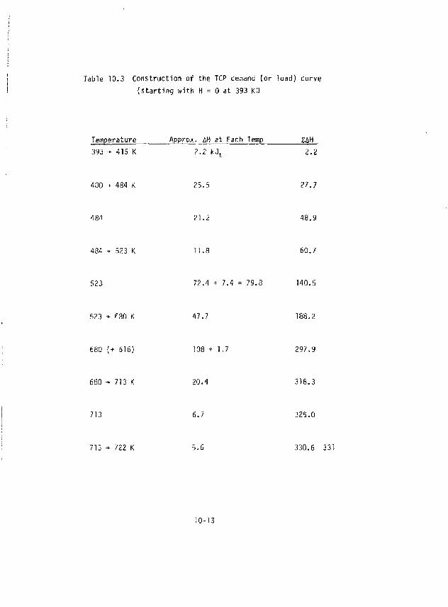
Table 10.3 Construction of the TCP demand (or load) curve (starting with H = 0 at 393 KO

Temperature flpprox. M at Each Temp ZAH 393 •* 415 K 2.2 kJt 2.2

400 -"• 484 K 25.5 27.7

481 21.2 48.9

484 523 K 11.8 60.7

523 72.4 + 7.4 = 79.8 140.5

523 - fSO K 47.7 188.2

680 (+ 616) 108 + 1.7 297.9

680 •» 713 K 20.4 318.3

713 6.7 325.0

713 •* 722 K 5.6 330.6 331

10-13

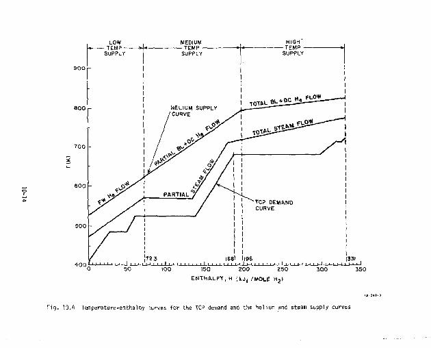
LOW •TEMP-

3 0 0 1 -

8 0 0

7 0 0

600

MEDIUM - TEMP -

SUPPLY

HIGH - T E M P -

SUPPLY

300 350

ENTHALPY, H t k o , /MOLE H 2>

F i g . 10.4 Temperature-enthalpy -urves f o r the TCP demand and the helium and steam supply curves

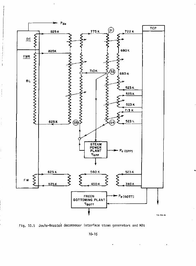
775K (§!) 722 K * • \L -*—>

TCP

680K

6 8 0 K

523 K

523 K

523 K

713 K

523 K

FREON BOTTOMING PLANT

''BOTT

pc (SPP)

523 K

393 K

" pe(BOTT)

Fig. 10.5 Joule-Boosted decomposer interface steam generators and HXs

10-15

yields high heat transfer coefficients and relatively low temperatures for the first wall structure. This results in desirably high allowable creep strength (see Section 5 for details).

The first-wall thermal power can be converted to kJ/mole Ho for plotting on Fig. 10.4 as follows:

E FW • Pjf^ * r § ? ° 7 2 - 3 k V m o l e

Using this value and the temperatures sited above, the low temperature portion of the helium supply curve can be drawn as shown at the left-hand side of Fig. 10.4 (defined as the "low temperature" region). The total first-wall helium flow rate required is thus calculated from:

^•i^-Sfirt'*''". (See Section 5 for further details.)

In order to construct the medium and high temperature portions of the helfjm supply curve, we first must choose helium blanket and direct converter coolant temperatures. After several iterations we found that reasonable helium inlet and outlet temperatures for adequately high /jT's between the sLesm and the helium were 625 K and 825 K, respectively, as indicated on rig. 10.5. These temperatures not only match the blanket design well, but also provide a low enough bulk temperature rise in the blanket canisters for good heat transfer without excessive pressure drops. It should be noted that these "high" temperatures for the J80 concept are much lower than the corresponding high helium temperatures for the FOB concept.

For the high temperature portion of the supply curve on Fig. 10.4, it was determined that the entire thermal power from the blanket and direct converters would >ave to be used. This conclusion was reached when it was determined that the total helium flow rate from the blanket and direct

10-16

converters was just sufficient to give the desired slope of the high temperature helium supply curve shown on Fig. 10.4 between 331 kJ/mole (at 825 K) and 198 kJ/mole (at 795 K). This slope results in adequately high aT's between the supply and demand curves at all points. This, in turn, helps insure that the steam generator designs will be cost effective.

The total helium flow rates for the selected bulk temperature rise of 200 K fur the blanket and direct converter flows are given by:

M = Pt(BL) „ (3360 - 285) x 1Q 6 _ „ „ . 6 L C AT p, e. , " 5200 x 200 ~ "*' K a / i

„ = /MDCJ_ a ^J4 B 404 kg/s DC c ATgCQ C. 5200 a 200 3

The choice of the point at which to stop using all the thermal power in the helium flow (at 795 K and 198 kJ/mole on Fig. 10.4} is not unique. Other choices would lead to slightly different helium supply curves and steam conditions, but these changes would have a minor effect on the TCP efficiency for this reference design.

Finally, the medium temperature thermal demands can be met by the partial helium power curve shown connecting the high and low temperature portions of the supply curve on Fig. 10.4. It should be noted that this choice is also not optimum (because the AT's are larger than necessary around 140 kJ/mole), but it does lead to simple steam generator arrangements.

Table 10.4 summarizes the helium thermal nowers available and required by the TCP in each temperature range. It can be seen that about 496 Mw t

from the blanket and direct converter helium flows is required to satisfy the medium temperature demands of the TCP. This leaves about 2475 lW t at helium temperatures from 795 K down to 625 K available tG produce steam for the electric power demands of the TCP. The steam flow requirements and the StPam supply curve which '.ve arrived at will be discussed next.

10-17

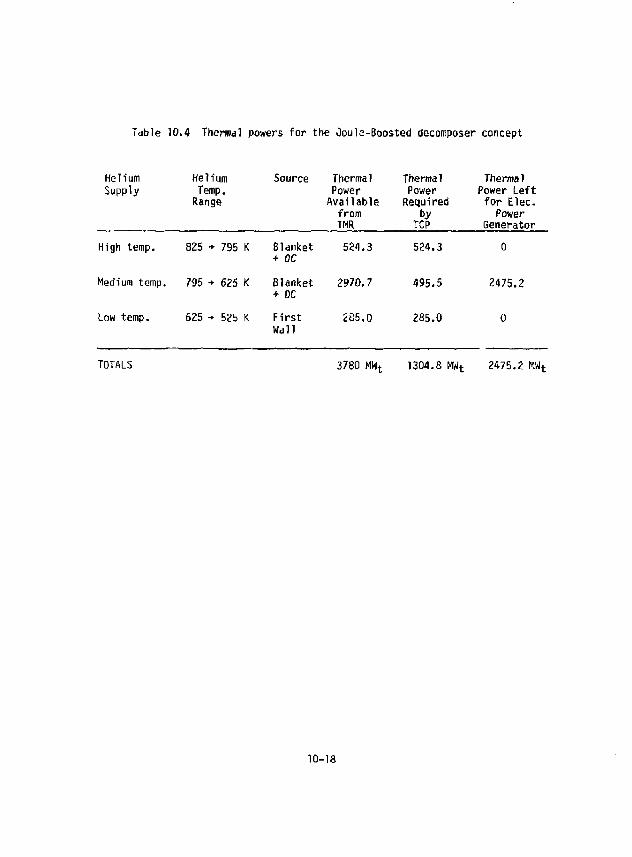
Table 10.4 Thermal powers for the Joule-Boosted decomposer concept

Helium Supply

Helium Temp. Range

Source Thermal Power Available from THR

Thermal Power Required

by TCP

Thermal Power Left for Elec. Power

Generator High temp. 825 + 795 K Blanket

+ OC 524.3 524.3 0

Medium temp. 795 + 625 K Blanket + DC

2970.7 495.5 2475.2

Low temp. 625 - 525 K First Wall

285.0 285.0 0

TOTALS 3780 MW+ 1304.8 MWt 2475.2 MW t

10-18

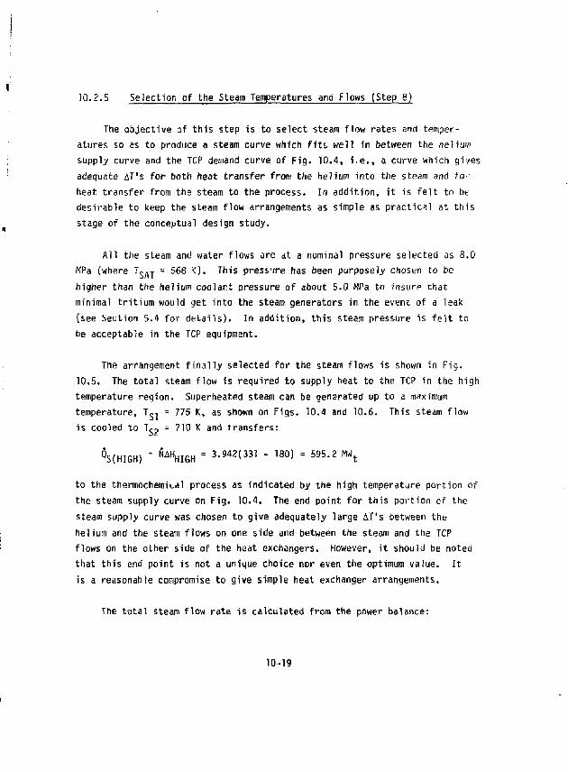
10.2.5 Selection of the Steam Temperatures and Flows (Step 8)

The objective of this step is to select steam flow rates and temper­atures so as to produce a steam curve which fits well in between the helium supply curve and the TCP demand curve of Fig. 10.4, i.e., a curve which gives adequate AT's for both heat transfer from the helium into the steam and fo-heat transfer from the steam to the process. In addition, it is felt to bt desirable to keep the steam flow arrangements as simple as practical at this stage of the conceptual design study.

All the steam and water flows are at a nominal pressure selected as 8.0 MPa (where T s - T = 568 <). This pressure has been purposely chosen to be higher than the helium coolant pressure of about 5.0 MPa to insure that minimal tritium would get into the steam generators in the event of a leak (see Section 5.4 for dfctails). In addition, this steam pressure is felt to be acceptable in the TCP equipment.

The arrangement finally selected for the steam flows is shown in Fig. 10.5. The total steam flow is required to supply heat to the TCP in the high temperature region. Superheated steam can be generated up to a maximum temperature, T g, = 775 K, as shown on Figs. 10.4 and 10.6. This steam flow is cooled to T<-, = 710 K and transfers:

^S(HIGH) ° " A HHIGH = 3 - 9 4 2 ( 3 3 1 " 1 8 ° ) = 5 9 5 - 2 M Wt

to the thermochemical process as indicated by the high temperature portion of the steam supply curve on Fig. 10.4. The end point for this portion of the steam supply curve was chosen to give adequately large AT's between the helium and the steam flows on one side and between the steam and the TCP flows on the other side of the heat exchangers. However, it should be noted that this end point is not a unique choice nor even the optimum value. It is a reasonable compromise to give simple heat exchanger arrangements.

The total steam flow rate is calculated from the power balance:

10-19

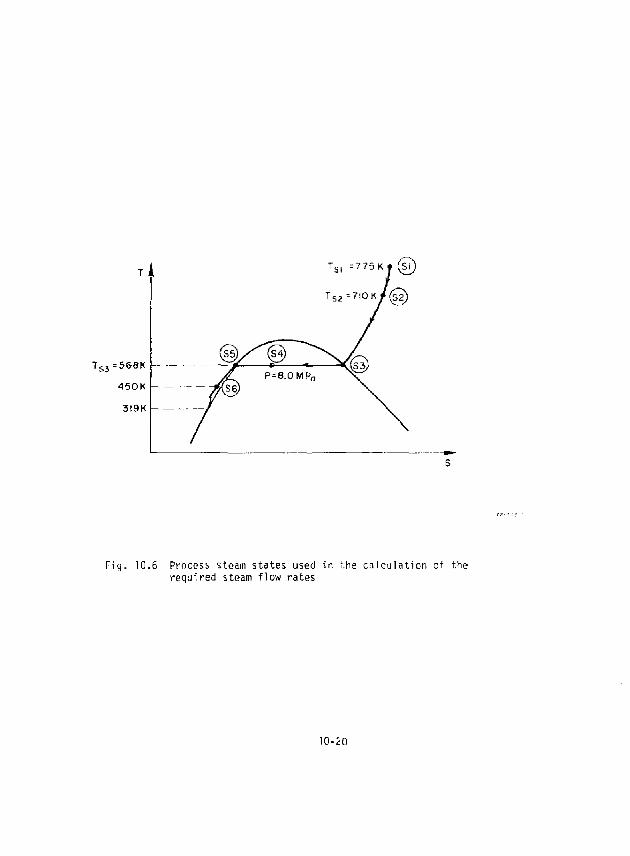
I

T *

450K

3I9K

T S | =775K • (S j )

T s 2 - - 7 l O K / ^ )

S5 S4

P = 8.0MF>„ .V.S3J

Fig. 10.6 Process steam states used in the ca lcu la t ion of the required steam flow rates

10-20

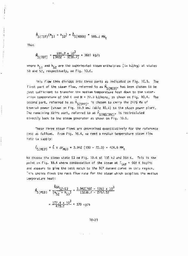
MS(TOT)<hSl " hS2^ = qS(HlGH) = 595.2 M»t

Thus

V o T ) = (3402*- 3236.7) " 3 6 Q l k g / s 595.2 x 10 3

where fv, and hv ? are the superheated steam enthalpies (in kJ/kg) at states SI and S2, respectively, on Fig. 10.6.

This flow then divides into three parts as indicated on Fig. 10.5. The first part of the steam flow, referred to as Mc/Mrn\» n a s been chosen to be just sufficient to transfer the medium temperature heat down to the satur­ation temperature of 568 K and H = 72.3 kJ/mole, as shown nn Fig. 10.4. The second part, referred to as M s, s„ p», is chosen to carry the 2475 MW of thermal power (shown on Fig. 10.3 an i Table 10.4) to the steam power plant. The remaining third part, referred to as Mc/ R E rTnr)> ^s recirculated oirectly back to the steam generator as shown on Fig. 10.5.

These three steam flows are determined quantitatively for the reference case as follows. From Fig. 10.4, we need a medium temperature steam f]ow rate to supply:

Q S ( M E D ) = N x A H M E D = 3.942 (180 - 72.3) = 424.6 MW t

We choose the steam state S3 on Fig. 10.6 at 135 kJ and 568 K. This is the point on Fig. 10.4 where condensation of the steam at r<-„T = 568 K begins and appears to give the best match to the TCP demand curve in this region. Tr.is choice fixes the mass flow rate for the steam which supplies the medium '.emperature heat:

N A H S2-S3 = 3.942(180 - 135) x 10 3

RS(MED) = T/h S 2 - h S 3 ) = (3236.7 - 2757/57

• ^imt^ - 37° *"*

10-21

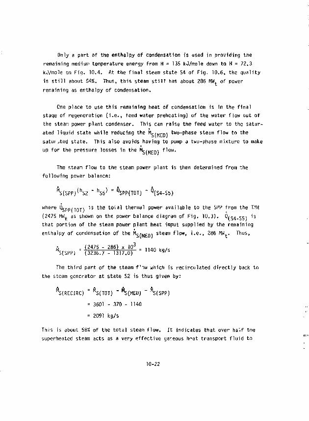
Only a part of the enthalpy of condensation is used in providing the remaining medium temperature energy from H = 135 kJ/mole down to H = 72.3 kJ/mole on Fig. 10.4. At the final steam state S4 of Fig. 10.6, the quality is still about 54%. Thus, this steam still has about 286 MW. of power remaining as enthalpy of condensation.

One place to use this remaining heat of condensation is in the final stage of regeneration (i.e., feed water preheating) of the water flow out of the steam power plant condenser. This can raise the feed water to the satur­ated liquid state while reducing the Mr(urn) two-phase steam flow to the satut ited state. This also avoids having to pump a two-phase mixture to make up for the pressure losses in the Mg/L,rD\ flow.

The steam flow to the steam power plant is then determined from the following power balance:

MS(SPP) ( hS2 " h S 5 } = ^SPP(TOT) " ^(S4-55)

where Q s p p , ,.„,-, is the total thermal power available to the SPP from the TMR (2475 MW. as shown on the power balance diagram of Fig. 10.3). Q(s4-55' l s

that portion of the steam power plant heat input supplied by the remaining enthalpy of condensation of the M s/ Hc n* steam flow, i.e., 286 MW.. Thus,

fl = (2475 - 286) x 10 3 = , „

S(SPP) (3236.7 - 1317.0) ' l , u K 9 / S

The third part of the steam f o w which is recirculated directly back to the steam generator at state S2 is thus given by:

MS(RECIRC) = ^SfTOT) " MS(ME0) " MS(SPP) = 3601 - 370 - 1140 = 2091 kg/s

This is about 58% of the total steam flow. It indicates that over half the superheated steam acts as a very effective gareous h^at transport fluid to

10-22

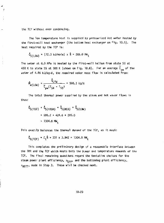
the TCP without ever condensing.

The low temperature heat is supplied by pressurized hot water heated by the first-wall heat exchanger (the bottom heai: exchanger on cig. 10.5). The heat required by the TCP is:

6^(!0W) = (72.3 kJ/mole) x ft = 285.0 Mkfc

The water at 8.0 MPa is heated by the first-wall helium from state S5 at 450 K to state S5 at 568 K (shown on Fig. 10.6). For an average ~C of the water of 4.86 kJ/kg-K, the required water mass flow is calculated from:

1 , m ^ • = — 598.3 kg/s Cpw<TS4 - V

w(LOW)

The total thermal power supplied by the steam and hot water flows in thus:

%(T0T) = ^S(HIGH) + QS(M£D) + qS(L0W) = 595.2 + 424.6 + 285.0 = 1304.8 MW t

This exactly balances the thermal demand of the TCP, as it must:

Q t ( T C p , = E tN '- 331 x 3.942 = 1304.8 MW t

This completes the preliminary design of a reasonable interface between the TMR and the TCP which meets both the pjwer and temperature demands of the TCP. The final remaining questions regard the tentative choices for the steam power plant efficiency, Tkp p ) and the bottoming plant efficiency, ^BOTT' m a c l e i n s t e p 3' T n e s e w1 il be checked next.

10-23

10.2.6 Estimation of the Power Plant Efficiencies (Stqp 9)

A simplified sketch of the steam power plant block diagram and cycle are given on Fig. 10.7. (Note that the steam cycle numbering on Fig. 10.7 is totally different from that for the process steam on Fig. 10.6.) The turbine receives the superheated steam flow M s/c p pv s.t state ) (710 K and 8.0 MPa) and expands it to state 2 in the high pressure part of the turbine. End state 2 is fixed by the maximum allowable moisture content of about 10%. Moisture is separated from the steam flow, which then flows to the medium pressure part of the turbine. The turbine from state 3 to state 6 -js very much like those designed for light water reactors and hence is conventional nuclear steam turbine technology, and the overall turbine is estimated to have an efficiency of 90%.

In addition to moisture removal from the steam flow, some steam is extracted at various points to preheat the compressed water from state 8 to state 9 (referred to as regene-ition), as indicated on the block diagram of Fig. 10.7. The final stage of the preheating from state 9 to stato 10 is accomplished using the medium temperature ..earn flow as described in Section 10.2.5.

The steam exiting from the turbine at state 6 is assumed to be condensed at about 0,01 MPa and 319 K. This temperature is high enough to permit use of conventional cooling towers.

Preliminary estimates of the thermal efficiency of this steam power plant indicate that it may be as high as 37% to 38% (compared to the guess of 35% on Fig. 10.3). Rather than redo the entire interface using an improved n.cPP (as recommended in Step 10), we will first evaluate the effect of small changes in the steam power plant efficiency on the overall thermo-chemical plant efficiency using a sensitivity analysis in the next section. Then if the effect on n-rri is large, a complete rtcalculc tion of the interface matching is probably justified. On the other hand, if the effect on n r r p is small, use of the results of the sensitivity analv .is to correct

10-24

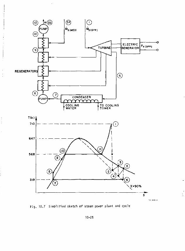
REGENERATORS

CONDENSER

COOLING WATER

ELECTRIC GENERATOR

P«(SPP)

©

wTO COOLING TOWER

T<k)

710

568

319

Fig. 10.7 Simpl i f ied sketch o f steam power plant and cycle

10-25

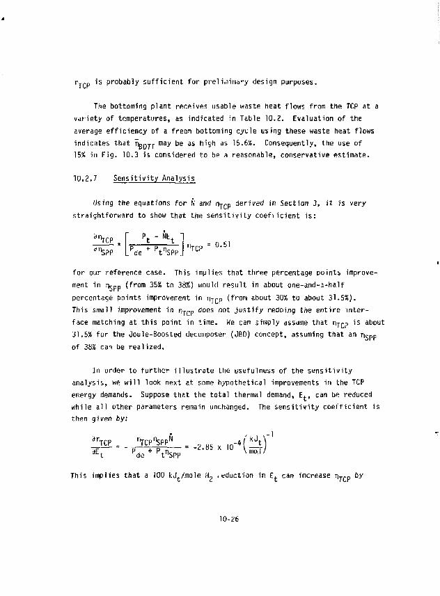
ru-(~p is probably sufficient for preliminary design purposes.

The bottoming plant receives usable waste heat flows from the TCP at a variety of temperatures, as indicated in Table 10.2. Evaluation of the average efficiency of a freon bottoming cycle using these waste heat flows indicates that TbQjy may be as high as 15.6%. Consequently, the use of 15% in Fig. 10.3 is considered to be a reasonable, conservative estimate.

10.2.7 Sensitivity Analysis

Using the equations for N and rwp derived in Section 3, it is very straightforward to show that the sensitivity coefiicient is:

r p

t-N i

' LPde + P t ^

>rhcp I vt - N E t ,nSPP | / d e + ' t ^ P P

n T C p = 0 . 5 1

for our reference case. This implies that three percentage points improve­ment in ncpp (from 35% to 38%) would result in about one-and-a-half percentage points improvement in riTrn (from about 30% to about 31.5%). This small improvement in pj^p does not justify redoing the entire inter­face matching at this point in time. We can simply assume that n^p is about S1.S% for the Joule-Boosted decomposer (JBD) concept, assuming that an n s pp of 3856 can be realized.

In order to further illustrate the usefulness of the sensitivity analysis, we will look next at some hypothetical improvements in the TCP energy demands. Suppose that the total thermal demand, E t, can be reduced while all other parameters remain unchanged. The sensitivity coefficient is then given by:

aiftp 'VCP'ISPP" , „ , v m-*(kJt\]

^ r " " pde+ •VSPT = - 2 - 8 5 * 1 0 w This implies that a 100 kj./mole H~ •eduction in E. can increase n T C p by

10-26

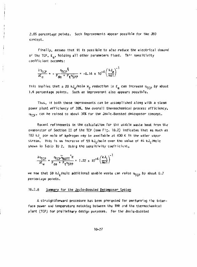
2.85 percentage points. Such improvements appear possible for the JBD concept.

Finally, assume that it is possible to also reduce the electrical demand he TCP, E , hole

coefficient becomes; of the TCP, E , holding all other parameters fixed. Thi*- sensitivity

3 n r C P - "TCP* - - 8 . U X 1 0 - 4 ' " ' 4 " 1

d E e Pde + ^ S P P mol/

This implies that a 20 kj^/ntole H^ reduction in Efi CQTI increase n-^p by about 1.6 percentage points. Such an improvement also appears possible.

Thus, if both these improvements can be accomplished along with a steam power plant efficiency of 38%, the overall tnermochemical process efficiency, rh-f-p, can be raised to about 36% for the Joule-Boosted decomposer concept.

Recent refinements in the calculation for the usable waste heat from the evaporator of Section II of the TCP {see Fig. 10.2) indicates that as much as 103 kj per mole of hydrogen may be available at 430 K in the water vapor stream. This is an increese of 59 kJt/mole over the value of 44 kJ-Vmole shown in Tabl? 10 2. Usirg the sensitivity coefficient,

3r>rcp ^CP^OTT'" . „ i n - 4 ^ V 3E„, _ P„ a + P.neoo " ' ' U * ' U Imol/ w pde + pt nSPP

we see that 59 kJ./mole additional usable waste can raise n-rrp b> about 0.7 percentage points.

10.2.8 Summary for the Joule-Boosted Decomposer System

A straightforward procedure has been prerented for performing the inter­face power and temperature matching between the TMR and the thermochemical plant (TCP) for preliminary design purposes. For the Joule-Boosted

10-27

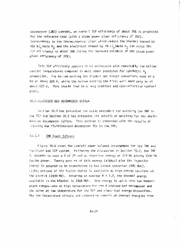
decomposer (JBD) concept, an overall TCP efficiency of about 30% is predicted for the reference case (with a steam power plant efficiency of 35%). Improvements in the thermochemical plant which reduce the thermal demand by 100 kJt/mole H„ and the electrical demand by 20 kj^/mole H 2 can raise the TCP efficiency co about 36% (using the improved estimate of the steam power plant efficiency of 38%).

This TCP efficiency appears to he achievable with remarkably low helium coolant temperatures compared to most other processes for synthetic H ?

production. The helium exiting the blanket and direct converters need only be at about 825 K, while the helium exiting the first wall need only be at about 625 K. This should lead to a 'e^y credible and cost-effective synfuel pi ant.

10.3 i-LuIOIZED BEL) UECOMPOSEK 5Y5Tti"!

Section 10.1 has presented the uasic procedure for matching the TMR to the TCP and Section 10.2 has presentee the details of matching for the Joule-Soosteri decomposer system. This section is concerned with the details of :.-!t.tcning the fluirlized-bed decomposer TCH to the TMR.

10.3.1 TMR Fower Balance

Mgure 10.8 shows the overall DQwer balance arrangement for the TMR and fiuidized bed TCP system. Following the discussivn in Section 10.2, the 7WP it assumed to have a fl of 25 and ar. injection energy of 140 MW giving 3500 •*' fusion power. Twenty perc.nt of this energy (alphas) plus the injection feierqy is assumed to be transferred to the direct converter (840 Mwt). : i'jhty percent of the fusion energy is available as high energy neutrons to the blanket (2800 MW). Assuming an average M = 1.2, the thermal energy available in the blanket is 3360 MWt. This energy is iplit into two temper­ature ranges--one at high temperature fn>- • he fluidized bed decomposer and the other at low temperature for the TCP and elect-ica! energy Production. The low temperature streams are assumed to consist of thermal energies from

10-28

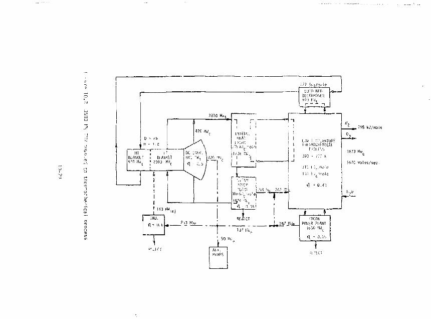
1 * FREON

PO'.itR PLANT 1650 MM

<l = 0 . 1 b r 1

'iJLCI

295 kJ/mole

673 N W o

5S7C moJes/sec,

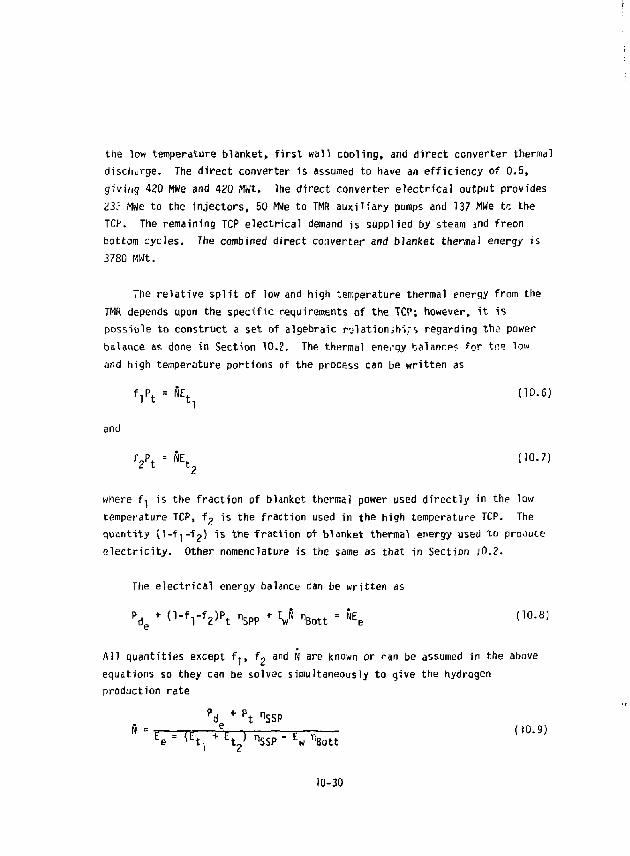
the low temperature blanket, first wall cooling, and direct converter thermal discharge. The direct converter is assumed to have an efficiency of 0.5, giving 420 MWe and 420 MWt. The direct converter electrical output provides 222 MWe to the injectors, 50 MWe to TMR auxiliary pumps and 137 MWe tc the TCK The remaining TCP electrical demand is supplied by steam and freon bottom cycles. The combined direct converter and blanket thermal energy is 3780 MWt.

The relative split of low and high temperature thermal energy from the TMR depends upon the specific requirements of the TCP; however, it is possible to construct a set of algebraic relationships regarding ths power balance as done in Section 10.2. The thermal energy balanr.es for tne low and high temperature portions of the process can be written as

Vt = \ < 1 0 - 6 >

and

f 2 P t = N E t 2 (10.7)

where fy is the fraction of blinket thermal power used directly in the low temperature TCP, f-j is the fraction used in the high temperature TCP. The quantity (1-fj-fo) is the fraction of blanket thermal energy used to produce electricity. Other nomenclature is the same as that in Section i0,2.

The electrical energy balance can be written as

\ + ( i - v v t i 5 P P

+ v 3 "Bo* = K < 1 0 - 8 )

All quantities except f,, f, and N are known or fan be assumed in the above equations so they can be solvec simultaneously to give the hydrogen production rate

P d + P t "SSP fi=? „ ~£_—, =—- (10.9)

E e = < E t . + E t 2 > ^SSP " Ew r '6ot t

10-30

The fractions f, and f ? can be calculated directly from Eqs. (10,6) and (10.7) once N is known. The plant efficiency can be ca culated from

^CP " P d + P t ( 1 0 - 1 0

10.3.? Energy Requirements of the Thermochemical Plant

Table 10.5 presents a summary of the thermal and electrical energy requirements for the system using the fluidized bed decomposer system. They are the same as for the Joule-Boosted system except for Section II of the TCP where high temperature thermal energy is used for the decomposer and its preheater. The distribution of energy for the various components in Section II also change because the conversion ratio for SO-, decomposition at 1100 (' is 65% as compared to &4% at 1250 K.

Figure 10.9 shows the energy inputs calculated* for the various components of Section II. The important point to be noted here is that the energy far the decomposer and its preheater is supplied by thermal energy from the high temperature blanket rather than by Joule (electric) heating. The recuperator provides, an important preheat and energy recovery function that separates the high and low temperature energy ranges.

The evaporator has two energy inputs as shown in Fig. 10.9. One is 29 kJ/mole from low temperature thermal energy and the other is 195 kj/mole from recovery of energy from the decomposer cooler. The evaporator energy requirement is calculated by assuming that 55% of the water can be condensed by pressure staging. Condensation of the remaining vapor permits a further energy recovery of 103 kJ/mole at 430 K. The other recoverable energies are listed in Table 10.6

* Appendix A presents details of the th ichemical calculations used for Section II.

10-31

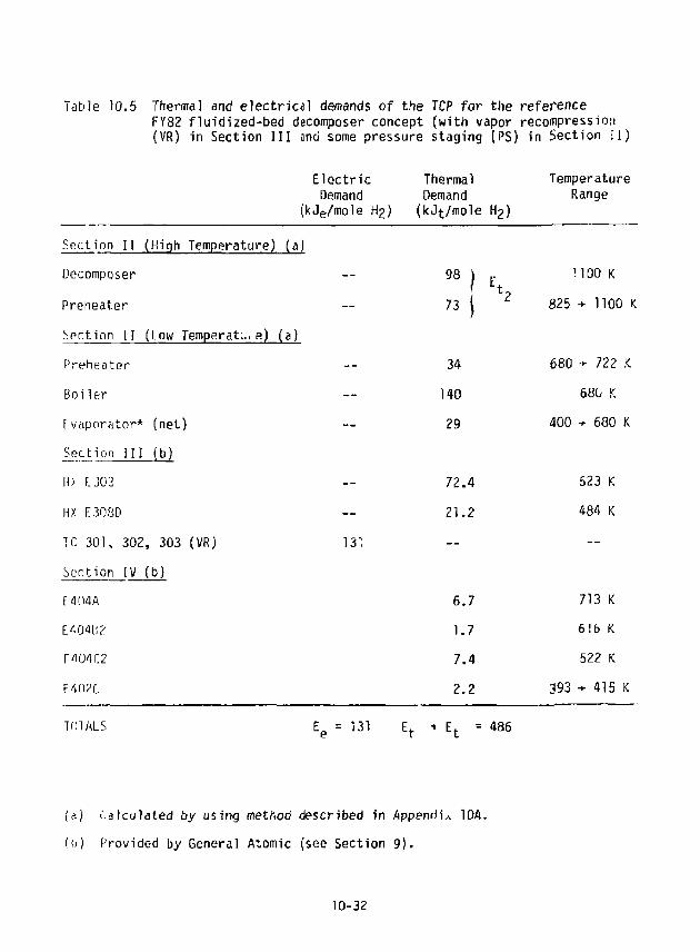
Table 10.5 Thermal and electrical demands of the TCP for the reference FY82 fluidized-bed decomposer concept (with vapor recompression (VR) in Section III and some pressure staging (PS) in Section II)

Electric Thermal Temperature Demand Demand Range

(kJe/mole Hz) (kJt/mole H 2)

Section II (High Temperature) (a) Decomposer

Preheater Section II (low Temperate e) (a) Preheater Boi lf;r Fvaporator* (net) Section III (b) H> F.J03 HX E308D TC 301, 302, 303 (VR) Section IV (b) E 4C14A E404H? E404C2 F40?C

131.

98 73 |

I h .

72.4 21.2

1100 K 825 + 1100 K

34 680 + 722 K 140 680 K 29 400 -* 680 K

523 K 484 K

6.7 1.7 7.4 2.2 393

713 K 616 K 522 K •* 415 K

£e = 131 Et * Et " 486 TOTALS

(a) i.alculated by using method described in Appendix IDA. (tj) Provided by General Atomic (see Section 9).

10-32

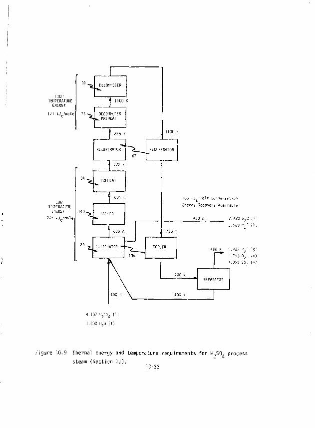
HIGH TEMPERATURE

ENERGY

DECOMPOSER

• 1100 K

DECOWi'ER * • h PREHEAT

RECUPERATOR

LOW Tf-IPERATL'SL

E'lER^Y

?03 k j . / no l e

*5_ pr.SiiEA

^ SO:LE»

29

^

•100 K

RECUPERATOR

!Cj ~J ' r o l e Co^conjat icn

Cne^cy Recovery Avai lable

430 K ?.J?0 K,C (n-:

Z.560 f - 3 { I .

733 •:

COOLER

400 k

100 >:

£ 1.533 S3 , ( c , 1

SEPARATOR

4 . 1 0 7 ' y . n , (1 )

f igure 10.9 Thermal energy and temperature requirements fo r H,SO. process steam (Section 11).

10-33

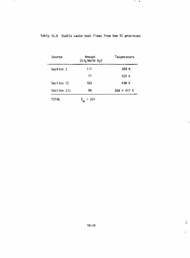
Table 10.6 Usable waste heat flows from the TC processes

Source Amount (k.Jt/iuole Hz) Temperature

Section I in 21

393 K 425 K

Section II 103 430 K Section III 56 368 + 417 K

TOTAL Ew = 2 9 1

10-34

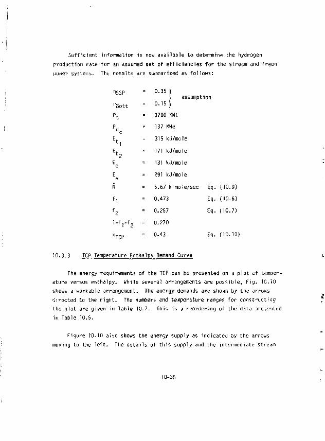
Sufficient information is now available to determine the hydrogen production rate for an assumed set of efficiencies for the stream and freon po^er systems. The results are summarized as follows:

^SSP

"Bott II II 0.35 |

J assumption 0.15 )

pt = 3780 MWt

X

£e

=

137 MWe

315 kO/mole

171 kJ/mole

131 kJ/mole

E w

= 291 kJ/mole

N = 5.67 k mole/sec Eq. (10.9)

fl = 0.473 Eq. (10.6)

h = 0.257 Eq. (10.7)

i-f rf 2 = 0.270

"-TPP = 0.43 Eq. (10.10)

10.3.3 TCP Temperature Enthalpy Oemand Curve

The energy requirements of the TCP can be presented on a plot of temper­ature versus enthalpy. While several arrangements are possible, Fiy. 10.10 shows a workable arrangement. The energy demands are sho^n by the arrows directed to the right. The numbers and te.nperature ranges for constricting the plot are given in Table 10.7. This is a reordering of the data presented in Table 10.5.

Figure 10.10 also shows the energy supply as indicated oy the arrows moving to the left. The details of this supply and the intermediate stream

10-35

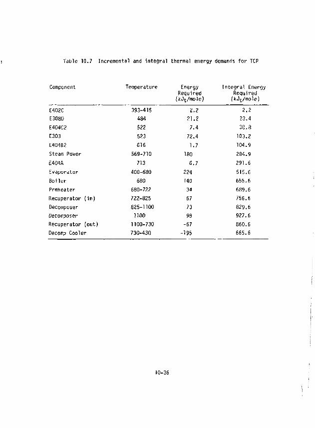
Table 10.7 Incremental and integral thermal energy demands for TCP

Component Temperature Energy Required (kJt/wle)

Integral Energy Required (J<Jt/mole)

E402C 393-415 2.2 2.2 E308D 484 21.2 23.4 E404C2 522 7.4 30.8 E303 523 72.4 103.2 E404B2 616 1.7 104.9 Steam Power 569-710 180 284.9 E404A 713 6.7 291.6 Evaporator 400-680 224 515.6 Boiler 680 140 655.6 Preheater 680-722 34 689.6 Recuperator (in) 722-825 67 756.6 Decomposer 825-1100 73 829.6 Decomposer 1100 98 927.6 Recuperator (out) 1100-730 -67 860.6 Decomp Cooler 730-430 -195 665.6

10-36

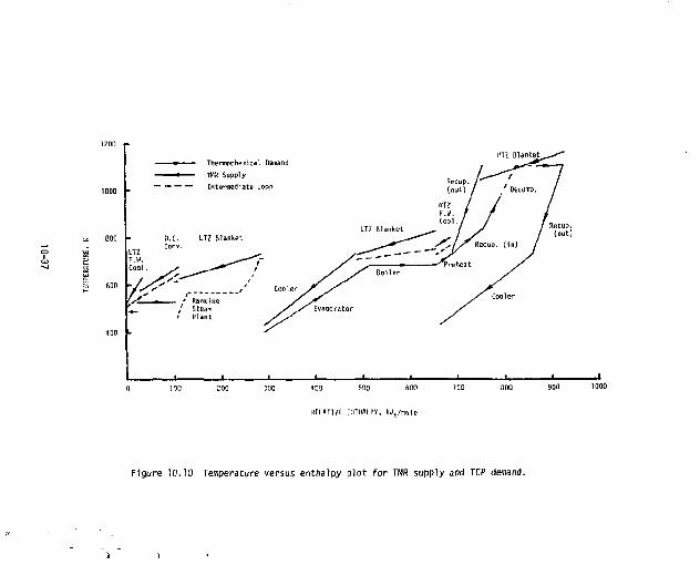
400 MO

RtUTlVf CrnilALP*. U t / n « l c

Figure 10.10 Temperature versus enthalpy plot for THR supply and TCP demand.

or water loops (dashed lines) are covered in the following section.

10.3.4 System Matching

Now that the energy demand curve has been constructed, it is necessary to construct a match with the energies available from the TMR and the energy recoveries in the TCP.

Table 10.8 summarizes the sources of thermal energy available to satisfy the process. The low temperature energy contribution totals to 495 kJt/mole which can satisfy the 315 kJt/mole used directly as thermal energy by the TCP and 180 kO^/mole which is used to make part of the electricity required for shaft work. The four low temperature energy sources represent four separate heat transport streams. Since two of them can be contaminated with tritium and they all have different temperature ranges, each heat transport stream is kept separate. Each source has its own heat transport loop and intermediate helium-to-steam (or water) heat exchangers to isolate the TMR from the TCP.

The high temperature energy stream is presently assumed to be directly coupled to the S0 3 decomposer and its preheater. The use of an intermediate heat exchanger could be of value here to provide some pressure staging, but would increase the blanket temperature unacceptably.

The TCP demands and the available thermal energies can be matched reasonably well by selecting comparable energy matches. The arrangement shown in Fig. 10.10 is a workable one and has reasonable temperature differences for the intermediate steam or water heat transport loops (dashed lines). The steam-Rankine power cycle is the same as that discussed in Section 10.2. The pressure is 8 MPa, saturation temperature of 568 K, and superheat to 710 K, as si.own in Fig. 10.7.

Figure 10.11 shows a schematic arrangement of the heat transport loops from the TMR, the intermediate steam (or water) isolation loops and the TCP

10-38

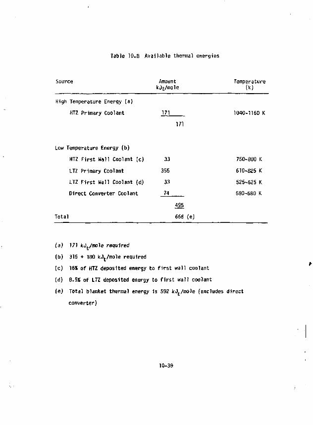
Source

Table 10.8 Available thermal energies

Amount kJfc/mole

Temperature W

High Temperature Energy (a) HTZ Primary Coolant 171

171 1040-1160 K

Low Temperature Energy (b) HTZ First Wall Coolant {c) LTZ Primary Coolant LTZ First Wall Coolant (d) Direct Converter Coolant

Total

33 750-800 K 355 610-825 K 33 525-525 K 74

495 666 (e)

580-680 K

(a) 171 kO./mole required (b) 315 + 180 kJt/mole required (c) 16* of HTZ deposited energy to first wall coolant (d) 8.5* of LTZ deposited energy to first wall coolant (ej Total blanket thermal energy is 592 kJt/mole (excludes direct

converter}

10-39

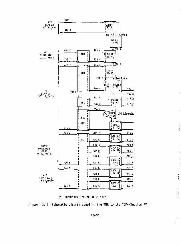
1160 K HTZ

BLANKET 171 kj /nole

HTZ FIRST HALL

LTI BLANKET

355 U t / raoIe

DIRECT CONVERTER

TliERML

LTZ FIRST WALL

U O O K

f 6*10 K 645 K 616 K

580 K 1 ^

I---1

1

-1 6"3 K

"IE40O2'" .(1.7)| 616 :<

580 K 1 ^

I---1

1

-1

643 K 523 K

580 K 1 ^

I---1

1

-1

559 K "J E303 f

523 K

580 K 1 ^

I---1

1

-1

559 K

"J E303 f

580 K 1 ^

I---1

1

-1

559 K 522 K

580 K 1 ^

I---1

1

-1

550 K lE4a4c?r '(7-4) J 522 :<

I™ , 625 K -i r

• i i i

* i i i i i ^ L

550 K 4ft4 :;

525 K

-i r • i i i

* i i i i i ^ L

514 K 1E308 O r

j(21.2)[ J L 484 K

525 K

-i r • i i i

* i i i i i ^ L

514 K 415 K

525 K

-i r • i i i

* i i i i i ^ L

510 K 1E402 cf 1(2.2) t 393 K

( * ) ENERGY TRANSFERS ARE Ifl kJ t / ; iOLE

Figure 10.11 Schematic diagram coupling the THR to the TCP—Section IV.

10-40

process loops. The temperatures indicated provide reasonable temperature differences for the heat exchangers involved.

10.3.5 Summary for the Fluidized Bed System

Figure 10.11 presents an overall summary of how the TMR is coupled to the TCP. The arrangement shown is workable, but it is not necessarily optimum. Better matching of the supply and load curves to reduce some of the larger temperature differences could provide a more optimum system.

The energy that must be generited in the high temperature blanket is 171 kJt/mole plus 33 kJf/tnole which is transferred to the first wall cooling. This is to be compared with the 592 kJt/mole totally supplied by the TMfi blankets.* This requires high temperature blanket coverage of 0.34 which is not obtainable with an overall tritium breeding ratio of 1.1 and where all breeding is done in the low temperature blanket. A more realistic fraction would be about 0.25. The impact is that the system matching must find additional high temperature energy or must use a decomposer and recuperator design that has better thermal energy use. One possible source of additional high temperatur energy is the thermal discharge from the direct converter. Assuming it could be designed to supply 74 kJt/mole over the temperature range from 825 to 1100 K, the decomposer would need 97 kJt/mole from the high temperature blanket. This would require a total of 135 ktL/mole to be deposited in the high temperature blanket to cover the 15% transferred to the first wall coolant. The result would be a drop in the energy fraction from 0.34 to 0.19, which is feasible.

The following conclusions can be made regarding the fluidized bed decomposer system:

1. A reasonable match exists such that the TMR can supply the thermal

* Total blanket thermal energy excludes direct converter thermal; 666-74=592.

10-41

and electrical energy demands of the TCP. This conclusion requires that the high temperature blanket provides 0.34 m of the total blanket thermal energy.

2, If the tritium breeding is limited to the low temperature blanket, the high temperature blanket energy must be supplemented from another source or the high temperature thermal demand of the decomposer must be reduced to allow a feasible match. Use of the direct converter thermal energy could reduce the high temperature blanket energy fraction to 0-19.

3. With resolution of the high temperature energy fraction issue, the system could achieve an overall efficiency of 43%.

10-42

APPENDIX 10.A

THERMOCHEMICAL CALCULATIONS FOR H 2S0 1 PROCESS STREAM - SECTION II

By 0. S. Rowe

As part of the University of Washington's support to LLNL, an independ­ent calculation was done to define the energy requirements for the hUSO^ process stream. The discussion presented here grew out of work done by Hark Abhold as part of a student design project and computations performed by Oscar Kirkorian at LLNL.

The calculations considered the H 2S0 4 process stream as represented by Fig. 10.A-1. The objective of the calculation was to calculate the energy requirement for each component based upon the enthalpy of the inlet and out­let streams. Each numbered stream could have up to 7 chemical species and the molar flow rates were defined based upon the chemical processes taking place in each of the components.

The total mass flow rate for each stream (j) was calculated from

where 'j n< .- = mole fraction of species i in stream j normalized to

production of 1 mole of hydrogen (mole,-/molen2); Mj = molecular weight of species i (g/mole); N = molar production rate of hydrogen (mole^/sec).

The s»ss balance for each component was calculated from

J J

10-43

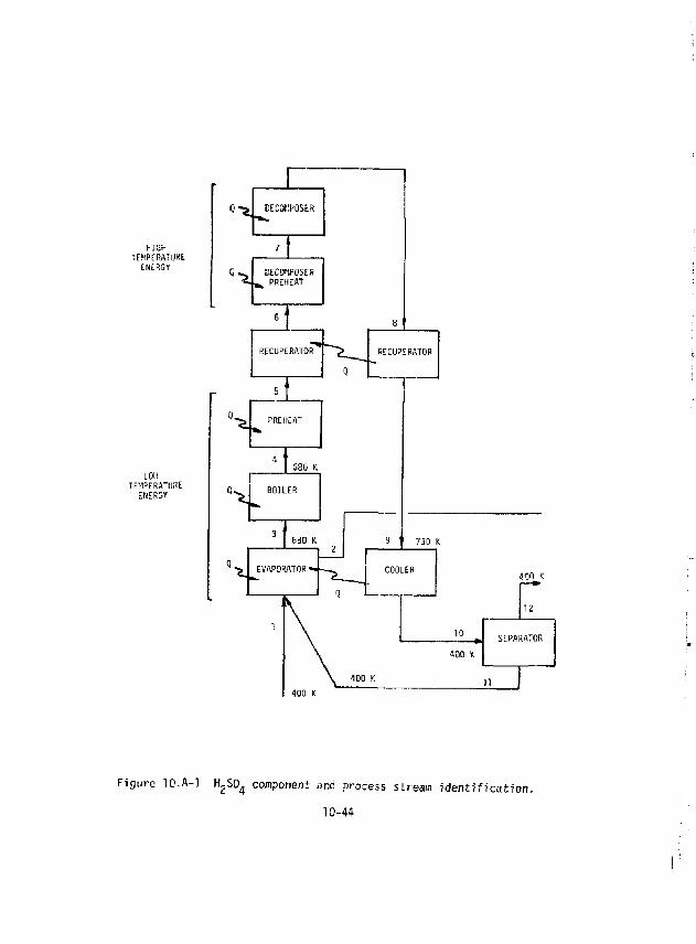
HIGH TEMPERATURE

ENERGY

LOU TEMPERATURE

ENERGY

Q - ^ DECOMPOSER

7

° ^ DECOMPOSER fc PREHEAT

6 8

RECUPERATOR

0

RECUPERATOR

5

S PREHEAT

4 ' 530 K

">. BOILER BOILER

3 680 K

2 9 730 C

EVAPORATOR -

2

COOLER V EVAPORATOR - COOLER 400 K

» 1

10 SEPARATOR

400 K

SEPARATOR

400 K

\ 400 K )) 400 K

Figure 10.A-1 f^SO^ component and process stream i d e n t i f i c a t i o n .

10-44

The stream enthalpy was calculated from

"j " ? ["l.J (hi " « + "t.J <

where h. •- mixture enthalpy of stream j ( M / m o l e ^ ) ;

h? - h?g 8 = enthalpy of species i above 298 K (kJ/mole-)

Ah2 = enthalpy of formation for species i (kJ/mole-)

The thermal energy requirement for each component was calculated from

q = N X (M t - 2 (M-Y j'ojt Y j m

where q = net thermal power (ktL/sec).

The enthalpy data for each species was taken from the JANAF tables.' ' The enthalpy of mixtures of liquid H20 and H SO,] was interpolated from the tables containing the various hydrates of HUSO^ and thus includes the enthalpy of mixing.

The molar flow rates for each species was taken from the compositions of (A2) Kirkorian^ ' and where the following assumptions were made for each stream:

Stream 1 - Input mixture of liquid H-SO^ and H~0 at 400 K.

Stream 2 - Partially condensed vapor (55%) as output from evaporator

available for energy recovery at 430 K.

Stream 3 - Azeotrope mixture of liquid H.,0 and HUSO,, at 680 K.

Stream 4 - Equilibrium molar composition of vapors {H?0, SO, ...) based ,'A21 on calculations of Krikorian. 1^'

Stream 5 - Same as Stream 4.

10-45

Stream 6 - Same as Stream 4. Stream 7 - Same as Stream 4. Stream 8 - SO., decomposition has occurred at the conversion ratio:

0.65 Fluid bed 1100 K 0.84 Joule-Boosted 1250 K

Stream 9 - Sensible cooling of decomposer products to 730 K only—no recombination of S0 ? and 0,.

Stream 10 - Cooling of products to 400 < without recombination of S0 2

and 0 2 but with recombinat'n.1 of SO, and H,0 to yield H-SO.. Stream 11 - Liquid H 20 and H 2 S 0 4 recycle at 400 K. Stream 12 - Product stream gases at 400 K.

The calculations were automated for a microcomputer and werp performed itera-tively to obtain stream temperatures that would allow energy matching of the recuperator. Stream temperatures, molar flow rates and enthaoy results for the fluidized bed and Joule-Boosted decomposers are presented in Tables 10.A-1 and 10.A-3. The energy requirement results are presented in Tables 10.A-2 and 10.A-4.

10-46

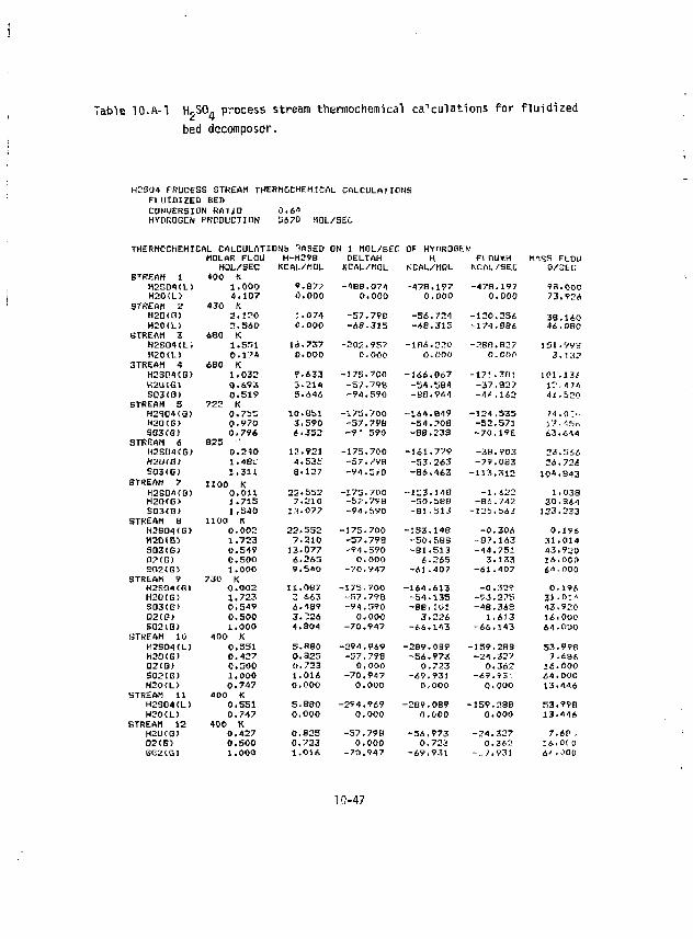
Table 10.A-1 H.-SO. process stream tHermochemical calculations for f luidized bed decomposer.

H2S04 PROCESS STREAM THERMGCHEMICAL CALCULATIONS FLUItUZED BED CONVERSION ftdllD 0.64 HYPROGEN PRODUCTION 5670 HOL/SEL

THEKMOCHEHICAL CALCULATION 7ASED ON 1 MOL/SFC OF HYriROGEN MOLAR FLOW H-H298 I'ELTAH H FLOU*H MftSS FLOW

MOL/SEC KCAL/MOL KCAL/MOL KCAL/MOL NCW./SEC S/SEC STREAM 1 400 K

H2S04<L> 1.000 9.877 -4BB.074 -478,197 -478.197 98.000 H20(L) 4.107 0.000 0.000 0.000 0.000 73.924

STREAM 2 430 K H2D<Q) 2.120 J. 074 -57.79B -56.724 -120.256 38.140 H20(L> 2.560 O.OQO -48.33 5 -68.335 -174.886 46.080

STREAM 3 680 K H2S04<L# 1.551 1A.737 -202.957 -136.220 -2B8.B27 1S1.99B H20(L) 0.174 O.OOO O.OOO 0.000 O.OOP 3, 132

STREAM 4 6B0 K H2S04CG> 1.032 9.633 -17E.700 -166.067 -17; .3fll 101.136 K2U(fi) 0.693 3.214 -57.79B -54.594 -37.827 12,474 S03((3> 0.519 5.646 -94.590 -BB.944 -4'.142 41,520

STREAM 5 722 K H2'304(G) 0.755 10.851 -17S.700 -164.849 -124.535 74.0"> H20CB> 0.970 3.590 -57.798 -54.208 -52.571 17,*,5D SOJfC) 0,796 4.352 -9• 590 -88.238 -70.19S 63.644

STREAM 6 825 H2SD4(G> 0.240 13.921 -175.700 -161.779 -38.903 23.566 H20<G) 1 .48;: 4.535 -57.798 -53.263 -79.083 26.724 S03<G) 1.311 8.127 -94.5T'0 -86.463 -113.312 104,843

STREAM 7 1100 K H2S04CG) 0.011 22.552 -175.700 -153.148 -1.422 1.038 H20(G> 1.715 7.210 -57.798 -50.588 -81.742 30.964 SD3(0> 1 ,540 13-077 -94.590 -B1.513 -325,563 123.233

STREAM 8 1100 K H2S04<G> 0,002 22.553 -175.700 -153.148 -0.306 0.196 H201G5 1.723 7.210 -57.798 -50.S8B -97.143 31.014 S03(G) 0.549 13.077 -94.590 -81.513 -44.751 43.920 P2CG) 0.500 6.265 0.000 4.265 3.133 16.000 S<T2<G> 1.000 9.S40 -70.947 -61.407 -61.407 64.000

STREAM 9 730 K H2S04CG) 0.002 11.0B7 -175.700 -164.613 -0.329 0. 196 H20(G! 1.723 Z 663 -S7.79B -54.135 -7J.275 35.014 SD3<G> 0.549 6.469 -94,590 -SB.101 -48.368 43.920 02(G> 0.500 3.126 0.000 3.226 1.413 14.000 S02CG) 1.000 4.S04 -70.947 -66.143 -66.143 64.000

STREAM 10 400 K H2S04(L) 0.551 5.880 -294.969 -289.0B9 -159.2BB 53.998 H20(G) 0.427 0.825 -57.798 -56.973 -24.327 7.486 02(G> 0.500 0.723 0.000 0.723 0.362 14.000 S02CG) 1.000 1,016 -70.947 -49,931 -69.95: 44.000 H20(L) 0.747 0.000 0.000 0,000 Q.OOO 13.446

STREAM 11 400 K H2S04(L) 0.551 S.S80 -294.969 -2B9.0B9 -159,28B 53.998 H20(L) 0.747 0,000 0,000 0,000 0.000 13.446

STREAM 12 400 K H2QCG) 0.427 0.825 -57,798 -56.973 -24.327 7.6P , 02(G) 0.500 0.723 0.000 0,723 0.362 16. 0< 0 S(12<G) 1.000 1.016 -70.947 -69.931 -.. 7.931 6' . JOO

10-47

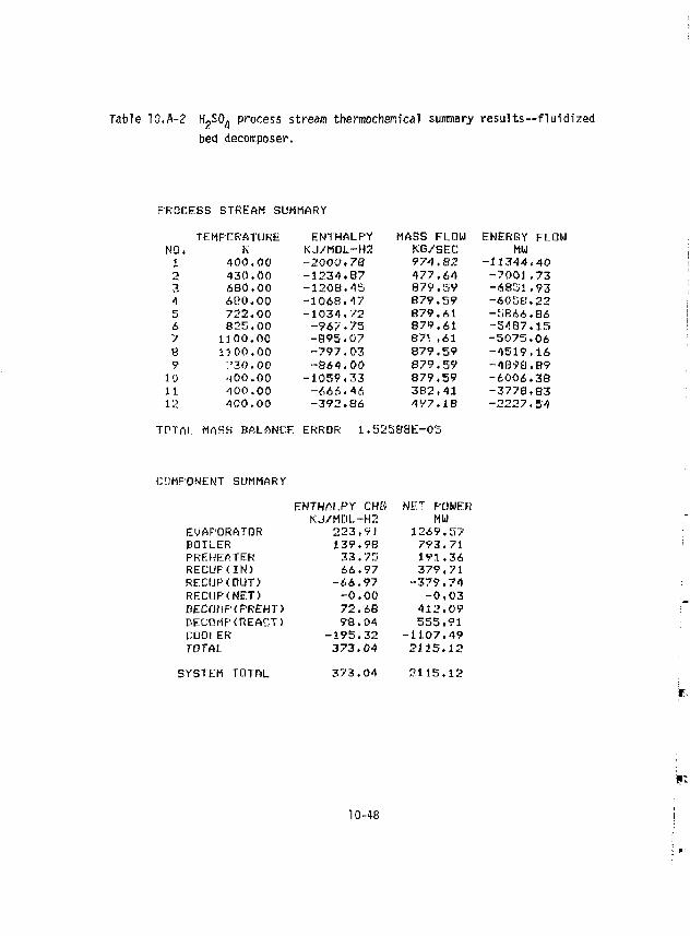
Table 10.fl-2 H2S0» process stream thermochenical summary results—fluidized bed decomposer.

PROCESS STREAM SUMMARY TEMPERATURE ENTHALPY MASS FLOW ENERGY FLOW

NO. K K J / M 0 L - H 3 KG/SEC m 1 4 0 0 . 0 0 - 2 0 0 0 , 7 6 9 7 4 . 8 2 - 1 1 3 4 4 . 4 0 •-} 4 3 0 . 0 0 - 1 2 3 4 . B 7 4 7 7 . 6 4 - 7 0 0 1 , 7 3 3 6 B 0 . 0 0 - 1 2 0 8 . 4 5 8 7 9 . 5 9 - 6 8 5 1 , 9 3 4 6 0 0 . 0 0 - 1 0 6 8 . 4 7 6 7 9 , 5 9 - 6 0 5 8 , 2 2 5 7 2 2 . 0 0 - 1 0 3 4 . 7 2 8 7 9 . 6 1 - 5 8 6 6 . 8 6 6 8 2 5 . 0 0 - 9 6 7 • 7 5 8 7 9 . 6 1 - 5 4 8 7 . 1 5 7 1 1 0 0 . 0 0 - 8 9 5 . 0 7 B 7 \ . 6 1 - 5 0 7 5 . 0 6 8 1 1 0 0 . 0 0 - 7 9 7 . 0 3 8 7 9 . 5 9 - 4 5 1 9 , 1 6 9 ' 3 0 , 0 0 - 8 6 4 . 0 0 S 7 9 . 5 9 - 4 8 9 8 . 8 9

10 •jOO.OO - 1 0 5 9 . 3 3 8 7 9 . 5 9 - 6 0 0 6 . 3 8 11 4 0 0 . 0 0 - 6 6 6 . 4 6 3 8 2 . 4 1 - 3 7 7 8 . 8 3 12 4 0 0 . 0 0 - 3 9 2 . 8 6 497,IB - 2 2 2 7 , 5 4

TPTAL MASS BALANCE ERROR 1 . 5 1 5 8 8 E - 0 5

COMPONENT SUMMARY ENTHALPY- CHE? N E T POWER

K J / M D L - H 2 MW EVAPORATOR 2 2 3 , 9 1 1 2 6 9 . 5 7 BOILER 1 3 9 . 9 8 7 9 3 . 7 1 PREHEATER 3 3 . 7 5 1 9 1 . 3 6 R E C U F U N ) 6 6 , 9 7 3 7 9 . 7 1 RECUR<OUT) - 6 6 . 9 7 - 3 7 9 . 7 4 REC(JP<NET) - 0 . 0 0 - 0 , 0 3 D E C t m P f P R E H T ) 7 2 . 6B 4 1 2 . 0 9 DECOMP<REACT) 9 8 . 0 4 5 5 5 . 9 1 COOLER - 1 9 5 . 3 2 - 1 1 0 7 . 4 9 TOTAL 3 7 3 . 0 4 2 1 1 5 . 1 2

YSTEM TOTAL 3 7 3 . 0 4 2 1 1 5 , 1 2

10-48

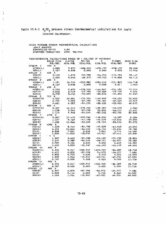
Table 10.A-3 H„SO. process stream thermochemical calculations for Ooule boosted decomposer.

H2SD4 PROCESS STREAM THERMOCHEMICAL CALCULATIONS JOULE BOOSTED CONVERSION RATIO 0.84 HTHRDGEN PRODUCTION 3940 MOL/SEC

THERMOCHEMICAL CALCULATIONS EASED ON 1 MOL/SEC OF HYTiROGEN MOLAR FLOU H-H298 DELTAH H FLOU*H MASS FLOU

MOL/SEC KCAL/MOL KCAL/MOL NCAL/MOL KCAL/SEC G/SEC STREAM 1 400 K

H2S04(U 1.000 9.877 -4BS.074 -478.197 -478.197 98-000 H20(L) 4.107 0.000 0.000 0,000 0.000 73,926

STREAM 2 430 K H20CQ) 2.120 1.074 -57.798 -56.724 -120.256 38.1if H20fL> 2.540 0.000 -68.3)5 -68.315 -174,B86 46.fJO

STREAM 3 680 K H2S04(L) 1.191 16.739 -202.982 -1B6.242 -221,815 116.7lB H20(LJ 0.134 0.000 0.000 0.000 O.OC ; 2.412

STREAM 4 680 K H2B04CG) 0.793 9.633 -175.700 -166.067 -131,691 77.714 H20(G> 0.532 3.214 -57.798 -54.SB4 -29,039 9.576 S03<G) 0.39B 5.646 -94.590 -88.944 -3S.400 31.840

STREAM 5 722 K H2S04CQ) 0.580 10.851 -175.700 -164.849 -95.630 56.830 H20<G> 0.745 3,590 -57.79B -54.208 -40.369 13.405 S03<G) 0.611 6,352 -9-4,590 -88.238 -53,905 48.672

STREAM 6 900 K H2S04(G> 0.067 16,213 -175,700 -159.487 -10.675 4.S60 H20(G> 1.238 5,240 -57,798 -52.558 -66.111 22.642 S03<G> 1.124 9,448 -94.590 -85.142 -95.705 89.925

STREAM 7 1250 K H2S04(G> 0.003 27.470 -175.700 -148.230 -0.33S 0.254 H2D(G) 1.322 B.769 -57.798 -49.029 -64.826 23,800 S03<G) 1.1B8 15,866 -94.590 -78.724 -93.556 95.072

STREAM 8 1250 K H20<G) 1.32S 8,769 -57."^e -49.029 -64.963 23.850 S03(G) 0.191 IS.866 -94.590 -78.724 -15.036 15.290 02(G) 0.500 7.541 0.000 7.541 3.771 16.000 S02(G) 1.000 11.536 -70.947 -S9.411 -59.411 64.000

STREAM i 0 K H20IG) 1.325 3.663 -57.798 -54.135 -71.729 23.BS0 S03IG) 0.19) 6.489 -94.590 -88.101 -16.827 15.280 02C3) 0.500 3.226 0.000 3.226 1.613 16.000 S02IG) 1.000 4.804 -70.947 -46.143 -46.143 64.000

STREAM 10 400 K H2SD4(L) 0,191 9.217 -459.947 -450.729 -86.039 18.713 H20CG) 0.427 0.825 -57.798 -56.973 -24.327 7.486 02<G> 0.500 0.723 0.000 0.723 0.362 16.000 S02IG) 1,000 1.016 -70.947 -69.931 -69.931 64.000 H20(L) 0.707 0.000 0.000 0,000 0,000 12.726

STREAM 11 400 K H2S04(L> 0.191 9.217 -459.947 -450.729 -86.089 18.718 H20CL) 0.707 0.000 0.000 0.000 0.000 12.726

STREAM 12 400 K H20<G> 0.427 0.825 -57.798 -56,973 -24.327 7.686 02(G) 0.500 0.723 0.000 0.723 0.362 16.000 302(G) 1.000 1.016 -70.947 -69.931 -69,931 64.000

10-49

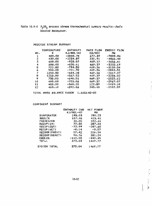
Table 10. A-4 '4,S0. process stream thermocherciical summary resul ts--Joule boosted decomposer.

PROCESS STREAM SUMMARY

TEMPERATURE ENTHALPY MAES FLOW ENERGY FLOW NO. K KJ/M0L-H2 KG/SEC MW 1 400.00 -2000.78 677.39 -7883.06 2 430,00 -1234.87 331.91 -4865.40 3 ABO.00 -92B.07 469.37 -3656.61 4 680.00 -820.61 469.37 -3233.19 5 722,00 -794.55 469.36 -3130.54 6 900.00 -721.70 469.36 -2843.51 7 1250.00 -664.28 469.36 -2617.27 8 1250.00 -567.52 469.37 -2236.02 9 730.00 -640.51 469.37 -2523.62 10 400.00 -753.06 469.37 -2967.07 11 400.00 -360.20 123.89 -1419.18 12 400.00 -392.86 345.48 -1547.B9

TOTAL MASS BALANCE ERROR 1.33514E-05

COMPONENT SUMMARY

ENTHALFY CHG NET POWER KJ/M0L-H2 MU

EVAPORATOR 198.03 780,23 BOILFTR 107,46 423,41 PREHEATER 26.05 102.66 RECUP(IN) 72.85 287.03 RECIJP(OUT) -72,99 -287.60 RECUPCNET) -0.14 -0.57 DECOMP(PREHT) 57.42 226.24 DECOMPtREACT) 96,76 381,24 COOLER -112.55 -443.45 TOT,,!. 373.04 1469.77

YSTEM TOTAL 373.04 1469.77

10-5C

References to Appendix 10.A

Al. JANAF Thermochemical Data, Dow Chemical, Midland, MI (data through 1979),

A2. 0. H. Krikorian, "Hydrogen Production Based on Magnetic Fusion," Lawrence Livermore National Laboratory, UCRL-86600 (1981),

10-51

SECTION 11.0 PRELIMINARY COST ESTIMATES

Contributor: L. Brown

TABLE OF CONTENTS

Section Description Page

11 .0 PRELIMINARY COST ESTIMATES 1 1 - 1

11.1 THE ECONOMIC BASIS 11-1

11 .2 COSTING PROCEDURES 11-2

11 .3 PRELIMINARY CAPITAL COST 11-3

11.3.1 Main Solut ion Reaction Step (Section I ) 11-3

11.3.2 H2SO4 Processing Step (Section I I ) 11-6

11.3.3 HI Concentration Step (Section I I I ) 11-6

11.3.4 HI Decomposition Step (Section IV) 11-10

11.3.5 Power Systems Inter face (Section V) 11-12

11.3.6 Fusion-Driven Nuclear Island 11-14

11.3.7 Summary of Capital Costs 11-14

11 .4 HYDROGEN PRODUCTION COSTS 11-18

11.4.1 Plant A v a i l a b i l i t y 11-18

11.4.2 Estimates of Hydrogen Production Costs 11-19

11.5 CONCLUSIONS ON PRELIMINARY COST ESTIMATES 11-23

REFERENCES 11-25

SECTION 11.0

List of Tables Table Page 11.3-1 Preliminary Capital Costs for Section I - M$, July 1980 . . . . 11-4

17.3-2 Preliminary Capital Costs for Section I I Based on the Joule Boosted Decomposer - M$, July 1980 11-7

11.3-3 Preliminary Capital Costs for Section I I Based on the

Fluid Bed Decomposer - M$, July 1980 11-8

11.3-4 Preliminary Capital Costs for Section I I I - M$, July 1980 . . . 11-9

11.3-5 Preliminary Capital Costs for Section IV - M$, July 1980 . . . . 11-11

11.3-6 Power Systems Section V Capital Costs (Fabricated, Instal led, and Indirect Costs) - M$, July 1980 11-13

11.3-7 Summary of Capital Costs for the Thermochemical Plant

and THR Fusion Driver - M$, July 1980 11-15

11.3-8 Capital Cost Estimate for 3500 MW fMR - M$ 11-16

11.3-9 Summary of Capital Costs for the Thermochemical Plant and THR Fusion Driver - H$, July 1980 11-17

11.4-1 Estimated Operating Cost of the Chemical Plant Sections I-IV Operating Costs Are Based on the Capital Cost of an Equivalent Chemical Plant Constructed of Mild Steel - H$, July 1980 . . . . 11-20

11.4-2 Estimates of Operating Costs and Hydrogen Production Costs of a TMR Driven Thermochemical Plant Based on the Joule Boosted Decomposer - H$, July 1980 11-21

11.4-3 Estimates of Operating Costs and Hydrogen Production Costs of a TMR Driven Thermocheniical Plant Based on the Fluid Bed Decomposer - H$. July 1980 11-22

n

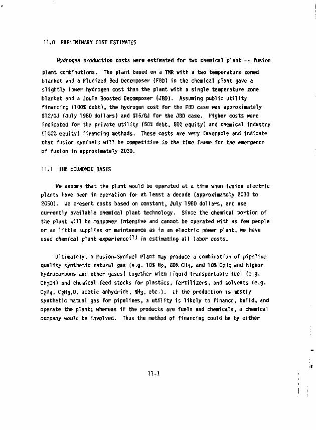
11.0 PRELIMINARY COST ESTIMATES

Hydrogen production costs were estimated for two chemical plant — fusion plant combinations. The plant based on a TMR with a two temperature 2oned blanket and a Fludized Bed Decomposer (FBD) in the chemical plant gave a slightly lower hydrogen cost than the plant with a single temperature zone blanket and a Joule Boosted Decomposer (JBD). Assuming public utility financing (100% debt), the hydrogen cost for the FBD case was approximately $12/GJ (July 1980 dollars) and J15/GJ for the JBD case. Higher costs were indicated for the private utility (502 debt, 50% equity) and chemical industry (100% equity) financing methods. These costs are very favorable and indicate that fusion synfuels will be competitive in the time frame for the emergence of fusion in approximately 2030.

11.1 THE ECONOMIC BASIS

We assume that the plant would be operated at a time when fusion electric plants have been in operation for at least a decade (approximately 2030 to 2050). We present costs based on constant, July 1980 dollars, and use currently available chemical plant technology. Since the chemical portion of the plant will be manpower intensive and cannot be operated with as few people or as little supplies or maintenance as in an electric power plant, we have used chemical plant experienced) in estimating all labor costs.

Ultimately, a Fusion-Synfuel Plant may produce a combination of pipeline quality synthetic natural gas (e.g. 10* H2, 80% CH4, and 10% CgH6 and higher hydrocarbons and other gases) together with liquid transportable fuel (e.g. CH3OH) and chemical feed stocks for plastics, fertilizers, and solvents (e.g. C2H4, C2H3.0, acetic anhydride, NH3, etc.). If the production is mostly synthetic natual gas for pipelines, a utility is likely to finance, build, and operate the plant; whereas if the products are fuels and chemicals, a chemical company would be involved. Thus the method of financing could be by either

11-1

utility (public or private) or chemical industry. We will present costs for these three kinds of financing.

17.? COSTING PROCEDURES

Both the ruifon community and chemical industy have developed considerable expertise in estimating the capital cost as well as the projected operating costs of their respective plants. The basis of TMR capital costs were independently derived at LLNlJ 2 ' whereas the TMR operating costs ar well as u t i l i t y financing are calculated in the manner specified by Ba t te l le ' 3 ' as the standard for fusion reactor conceptual designs.

The hydrogen production rate of the Joule Boosted Decomposer/Moderate Temperature Blanket based hydrogen plant is signif icantly lower than that of the Fluid Bed Decomposer/Two-Zone Blanket. Complete design of two different chemical plants was avoided by designing a standard size chemical plant and scaling the results to the two different cases. The standard plant, producing 4900 moles per second of hydrogen, is the same size as that reported last year f 4 ' . A significant fraction of the plant is unchanged from last year (Sections I , IV and part of I I I ) and thus was not recosted. Section I I was hosted separately for both the Joule Boosted and Fluid Bed Decomposer concepts. The size of the chemical plant is such that multiple parallel trains are used throughout most of the plant; therefore, a l inear scaling law was used to produce cost estimates for the resized plants.

Costs for the Chemical Plant and the power systems Interface are obtained by standard chemical engineering costing techniques. These costing techniques are based upon using actual construction experience from many chemical plants to predict capital and operating costs from FOB equipment costs. The new reference work by Peters and Tlmroerha^ 1) was used to augment the older Guthrie methods(5,6) both for estimating the FOB costs of equipment, as well as deriving from the FOB cost estimates of the Installed direct capital cost,

IT-?

the total plant investment and the operating cost. Where standard works could not provide capital costs, as in most of Section II and the power recovery systems, vendor estimates or other special sources of FOB cost data were used. The industry standard, Marshall and Swift (H«S)^), equipment cost index was used to reduce all costs to the same basis, July 1980.

It is recognized that some of the best costing techniques are maintained as proprietary by A8E, chemical and oil companies. A proprietary costing method, available at GA was used to spot check costs for a representative number of items. No overall bias could be observed although variations between different types of equipment \<eva noted.

We besieve that our cost estimates are well within our goal of •+ 30$ accuracy.

11.3 PRELIMINARY CAPITAL COST

11.3.1 Main Solution Reaction Step (Section I)

The simplified schematic of Section I was presented in Figure 9.3-1. Table 11.3-1 presents a detailed list of the equipment required for performing the main solution reaction step, together with size -*nd cost data. With the exception of the Heat Exchanger Reactor (R-101), all items have been costed by the Guthrie method.<5»^'

The structural material used throughout Section I is mild steel. If other than dry SO2, oxygen and or water are present, the steel must be protected by an appropriate coating or lining. Although spray on hydrocarbon based coatings are adequate when moist SO2 is present, liners of bulk fluorocarbon are specified when H2SO4, HI or I2 are present. The installed cost of fluorocarbon linings is estimated to be $V.00/m2.

11-3

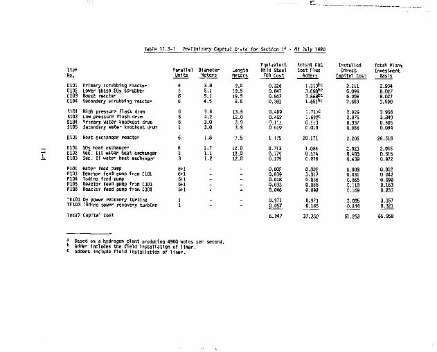
Table 11.3-1 Preliminary Capfta! Cr^ts for Sectfcn r a MS .July 1980

Item No.

ClOl C102 C103 C104

S101 S102 S104 S10S

Primary scrubbing raactor Lower phase SO? scrubber Boost reactor Secondary scrubbing reactor High pressure flash drum Low pressure flash drum Primary water knockout drum Secondary water knockout drum

R101 Heat exchanger reactor E101 SO2 heat exchanger E102 Sec. Ill water heat exchanger E103 Sec. II water heat exchanger PIQl Water feed pump P103 Reactor feed pump from ClOl P1D4 Iodine feed pump P105 Reactor feed pump from C103 P106 Reactor feed pump from C103 TE101 02 power recovery turbine TE103 Iodine power recovery turbine Total Capital Cost

Parallel Units

Diameter Meters

Length Meters

Equivalent Mild Steel

FOB Cost

Actual FOB Cost Plus

Adders

Installed Direct

Capital Cost

Total Plant Investment

Basis

6

6 6

3.8 5.1 5.1 4.5

9.0 19.5 19.5 8.6

0.326 0.847 0.847 0.381

1.353 b c

3.868 b c

3.868b<: 1.651 b c

2.211 6.096 6.096 2.653

2.934 8.027 8.027 3.508

6 6 6 1

3.6 4.2 3.0 3.0

13.5 12.0 3.9 3.9

0.489 0.452 Q.l 'J 0 019

1.743": 1.692= 0.113 0.019

2.929 2.875 0.337 0.056

3.956 3.849 0.505 0.084

6 1.8 7.5 1.175 20.171 2.206 26.518

6 2 3

1.7 1.1 1.2

12.0 12.0 12.0

0.713 0.174 0.276

1.084 0.174 0.276 HI

2.945 0.615 0.972

S+l 6+1 6+1 6+1 6+1

:

: 0.002 0.009 0.018 0.033 0.046

0.002 0.017 0.036 0.066 0.092

0.008 D.031 0.065 0.118 0.169 III

II

1 1 _ _ 0.971

0.057 0.971 0.165

2.095 0.244

3.157 0.321

6.947 37.350

^ Based on a hydrogen plant producing 4900 moles per second. b Adder includes the field installation of Uner. c Adders include field installation of l iner .

The Heat Exchanger Reactor is unique because of the material involved, niobium. The $220/kg cost of the niobium tubing dominates the reactor cost. Added to the $15.8M cost of the tubing is an appropriate amount for installation of the tubing ($3.2M), plus the FOB cost of the equivalent mild steel heat exchangers ($1.2M1, giving and FOB cost of $20.2M. Installation cost was estimated from the cost of the equivalent mild steel heat exchanger since niobium is required only for the heat transfer surfaces.

The Guthrie method allows specification of the piping materials separate from the specification of the materials of construction of the equipment. Either mild steel or standard fluorocarbon lined mild steel piping was specified as appropriate. Pumps are either cast iron for water, or cast iron with a molded fluorocarbon liner for corrosive solutions.

Since Section I operates essentially as six systems in parallel, 83% of production capacity may be maintained if any one system Is down for repairs. Pumps are cross-connected such that one installed spare backs up the active six. The power recovery turbines are not spared except by a by-pass valve.

The column labeled "Total Plant Investment Basis" is Table 11.3-1 indicates that the major unit costs of Section I are associated with the Heat Exchanger Reactor (R-101). The cost of R-101 may be decreased if more of the heat load is shifted to water-based heat exchangers. If the power bottoming cycle were eliminated the cost of R-101 would be significantly decreased due to the much larger differential temperatures across the exchanger.

11-5

11.3.2 H2SO4 Processing Step (Section I D )

The simplified schematics for the Joule Boosted Decomposer were presented in Figures 9.4-1 and 9.4-2. Detailed lists of the equipment required for H2SO4 conc> ntration and decomposition together with cost data are presented in Tables 11.3-2 and n.3-3 for these two cases. All cost estimates were made using Guthrie's techniques'5,6) except for the decomposers. Details of the decomposer cost assumptions were presented in last year's report''*'.

The major costs in Section II are associated with heat transfer equipment. Silicon carbide is the material of choice for heat transfer surfaces where liquid-gas interfaces occur. Silicon carbide is used for all heat transfer involving coti^etrated sulfuric acid except in the Recuperator/Decomposer Preheater. Inco;oy--800H is used in the Recuperator/Decomposer Preheater as only gases exist at the temperatures encountered.

Vessels are fabricated from Fluorocarbon-lined mild steel, with this lining thermally insulated from the process via acid brick linings. At the higher acid concentrations, steel is passivated; and the fluorocarbon linings are unnecessary.

Costs of silicon carbide and vessel liners are treated as adders to the base carbon steel equipment costs. Silicon carbide U-tube costs are estimated to be $ 3 2 . 7 / H ' 8 ' for the 5 cm diameter tubes specified for the H2SO4 vaporizjr, and this cost was used in estimating the rest of the silicon carbon heat exchangers.

11.3.3 HI Concentration Step (Section III)

Capital costs for Section III are presented in Table 11.3-4. The simplified flow diagram for this section was presented in Figure 9.7-1.

11-6

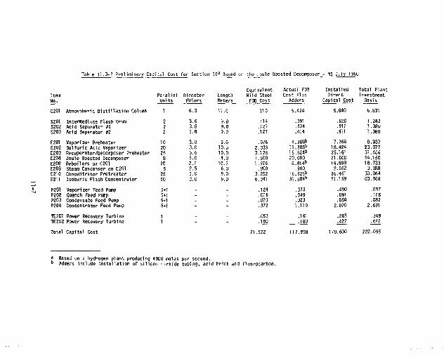
Table 11.3-2 Prel iminary Capital Cost f o r 5ect ion I I a Based on the Joule Boosted Decomposer - M3 Quly 198Q

Hem Ho.

C201 Atmospheric Distillation Column

SZ01 Intermediate Flash Drum SZ02 Acid Separator #2 S203 Acid Separator K

E201 Vaporizer Preheater E202 Sulfuric Acid Vaporizer E203 Recuperator/Decomposer Preheater E204 Joule Boosted Decomposer E208 Reboilers on C201 E209 Steam Condenser on C201 E210 Concentrator Pretreater E211 Isobyric Flash Concentrator

P201 Vaporizer Feed Pump P202 Quench Feed Pump P203 Condensate Feed Pump P204 Concentrator Feed Pump

TE201 Power Recovery Turbine TE202 Power Recovery Turbine

Tata! Capital Cost

2 2 2

10 20 25 8 20 5 25 50

5+1 5+1 5+1 5+1

3.6 3.8 3.a

3.0 3.0 5.6 3.0 2.1 2.5 3.0 3.0

Lengtii Meters

9.0 9.0 9.0

9.0 10.u 10.0

4.0 10.7

6.0 9.0 9.0

Equivalent Mi ld Steel

FOB Cost

. l i t

.127

.127

.976 2,333 3.125 1 .500 1.976

.900 3.252 6.341

.124

.016

.023

.372

.053

.180

Actual F00 Cost Plus

Adders

.391

.434

.434

I I . 3 0 S b

15.524t> 20.000 8.814 b

.900 16.525 b

31.B04 b

.373

.049

.023 1.119

.161

.180

Ins ta l l ed Total Plant D i rec t investment

Capital Cost _ Basis

.820

.911

.911

7.366 18.424 25.161 21.000 14.898

2.052 26.461 51.159

.690

.097

.054 2.070

.265

.427

178.600

1 .242 1.38U 1.380

8.937 23.077 31.436 24.150 18.733

3.088 33.064 63.968

.897

.118

.082 2.691

.349

.642

a Based on a hydrogen plant producing 4900 moles per second. D Adders include installation of silicon r.>rbide tubing, acid brick and fluorocarbon.

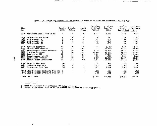
Table 1 1 ,

Item Ho.

C201 Atmospheric D i s t i l l a t i o n Column

5201 Intermediate Flash Drum 5202 Acid Separator #1 5203 A d a Separator #2 5204 Acid Separator #3

E201 Vaporizer Pretreater E202 Su l f u r i c Acid Vaporizer E203 Recuperator/Decomposer Preheater E204 F lu i d Bed Decomposer E20B Rebollers on C201 E209 Steam Condenser on C201 E21Q Concentrator Preheater EZ11 Isobar ic Flash Concentrator

P201 Vaporizer Feed Pump P203 Condensate Feed Pump P204 concentrator Feed Pump

TE201 L iqu id Expander-Condensate from C202 TE2Q2 L iqu id Expander-Condensate from S201

i p l t a l cost f o r section I l a Base d on the F l u i d 1 3ed Decomposer - M», Ouly 1980

Equivalent Actual FOB Ins ta l led Total Plant Para l le l CM ameter Length Mi ld Steel Cost Plus Di rect Investment

Units Meters Meters FOB Cost Adders Capital Cost Basis

1 7.0 11.0 0.147 7.882 7.732 9.044

2 3.6 9.0 .114 .391 .820 1.242 2 4.4 9.0 .168 .575 1.206 1.827 2 4.4 9.0 .168 .575 1.206 1.827 2 4.4 9.0 .168 .575 1.206 1.827

10 3.0 10.0 1.142 s.ia*** 8.618 10.456 20 3.2 10.0 2. 13.2270 21.556 27.000 25 5.6 10.0 3.125 15.624 25.16! 31.466

7 6.0 10.0 10.000 45.000 50.000 57.500 20 2.3 10.7 2.312 10.312" 17.431 21.918

5 2.5 6.0 .900 .900 2.052 3.088 25 3.0 9.0 3.252 16.535" 26.461 33.064 E0 3.3 9.0 6.341 31.804 51.159 63.968

5+1 _ w .124 .373 .690 .897

5+1 - - .023 .023 .054 .082 5+1 - - .372 1.119 2.070 Z.691

D2 I _ _ .053 .161 .265 .349 01 1 - - .180 .180 .427 .642

Total Capi ta l Cost 269.006

j* Based on a hydrogen plant producing 4900 moles per secoiid. b Adders include Installation of silicon carbide tubing, acid brick and Huorocarbn^.

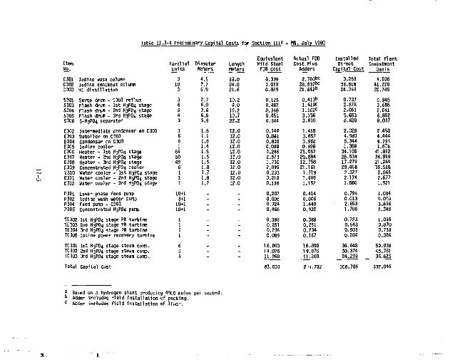
Table U.3-4 prel iminary cap i ta l costs for Section 111° - MS, Ju ly 1980

Item N i l

C301 Iodine wash column C302 iodine knockout column C303 HI d i s t i l l a t i o n

$301 surge drum - C303 r e f l u x 5303 Flash drum - 1st H3PO4 stage 5304 Flash dram - 2nd H3PO4 stage 5305 Flash drum - 3rd HjP0<, stage 5306 S-H3PO4 separator

E302 Intermediate condenser on C303 E303 Reboiler on C303 E304 Condenser on C303 E305 Iodine cooler E306 Heater - 1st K3PO4 stage E307 Heater - 2nd H3PO4 stage E308 Heater - 3rd K3PO4 stage E309 Concentrated H3PO4 cooler E31D Water cooler - 1st H3PO4 stage E311 Water cooler - 2nd H3PO4 stage E312 water cooler - 3rd H3PO4 stage

P301 Lower phase feed pump P30Z Iodine wash water pump P304 Feed pump - C303 P305 Concentrated H3PO4 pump

TE302 1st H3PO4 stage PR turb ine TE303 2nd H3PO4 stage PR turb ine TE304 3rd H3PO4 stage PR turb ine TE305 Iodine power recovery turbine

TC301 1st H3PO4 stage steam comp. TC302 2nd H3PO4 stage steam comp. TC303 3rd H3PO4 stage steam coup.

Total Capital Cost

a Based on a hydrogen plant producing l

b Adder includes f i e l d i n s t a l l a t i o n of . c Adder includes f i e l d i n s t a l l a t i o n of 1

Equivalent Parallel Di ameter Length M1ld Steel Units Meters Meters FOB cost

3 4.5 18.0 0.339 10 7.7 24.0 3.059 3 6.9 21.6 0.889

3 2.7 10.2 0,125 G 6.0 9.0 0,487 5 3.6 16.2 0.348 4 6.6 10.7 0.451 3 5.9 22.2 0,544

3 1.6 12.0 0.144 6 1.1 12.0 0.881 6 1.6 12.0 0.800 1 1.4 12.0 0.099

65 1.5 12.0 3.246 50 1.5 12.0 2.573 49 1.5 12.0 1.730

6 1.8 12.0 2.095 1 1.7 12.0 0.233 1 1.8 12.0 0.218 1 1.7 12.0 0.IS6

10+1 _ . 0.207 3+1 _ _ 0.006

10+1 _ - 0.724 10+1 - - 0.456

1 _ _ 0.338 1 _ _ 0.251 1 - - 0.234 1 - - 0.0B5

6 _ _ 16.890 5 _ - 14.075 4 11.260

63.003

moles per second, c ing.

Actual FOB Ins ta l led Total Plant Cost Plus Direct Investment

Adders Capital Cost Basis

2.70QOC 3.253 ,_B36 28.537°c 33.618 41.220 21.642" 24-394 28.745

0.413b 0.737 0.945 1.619C 2.876 3.686 1.162= 2.061 2.641 3.156 5.653 6.852 3.810 6.620 8.037

1.459 2.029 2.450 3.853 4.983 6.444 3.962 5.344 6.7S4 0.998 1.388 1.676

25.057 34.105 41.852 20.884 28.534 34.899 12.758 17.279 21.269 21.161 29.418 35.528

1.719 2.327 2.865 1.606 2.174 2.577 1.152 1.560 1.921

0.414 0.794 1.084 O.0O6 0.013 n.O'.'O 1.449 2.653 3.656 0.932 1.706 2.346

0.388 0.723 1.065 0.2S1 0.548 0.870 0.234 0.503 0.738 0.167 0.284 0.386

16.890 36.448 59.938 19.075 30.374 45.781 11.260 24.299 35.625

2 ;l.732 306.706 397.046

Materials of construction and costing techniques are similar to those of Section 1. Where, because of thermal or mechanical limitations, fluorocsrbon linings are not acceptable, we have used Hastelloy-C.

The hydrogen iodide concentration step is the most capital intensive portion of the chemical plant. Although significant costs are associated with iodine knockout and hydrogen iodide distillation, the largest costs are associated with phosphoric acid concentration.

The high cost components of the phosphoric acid concentration system are steam compressors and heat exchangers. The compressor costs are based on vendor estimates'9^ and reduced to the 1980 base using the M<SS^7) cost index. These compressor costs appear to be fixed unless future developments bring down the relative cost of turbine compressors. Flowsheet modifications have the potential for reducing the heat transfer costs, particularly if direct contact heat transfer is employed between immiscible streams in Sections I and III and between Sections III and IV. The large amount of rotating machinery in the phosphoric acid concentration system makes this part of the process a potential soi'rce of downtime. The compressors in the third evaporation stage were deliberately oversized to make them identical to the first and second stage units. If any one of the 15 units is down, intermediate pressures may be shifted to permit operation at 93% of capacity with only a slight overall efficiency loss.

11.3.4 HI Decomposition Step (Section IV)

The HI decomposition step has the lowest flow rates and lowest costs of the four chemical process steps. The costs are as high as given in Table 11.3-5 only because of the high pressures involved. The simplified flowsheet for Section IV was given in Figure 9.8-1.

11-10

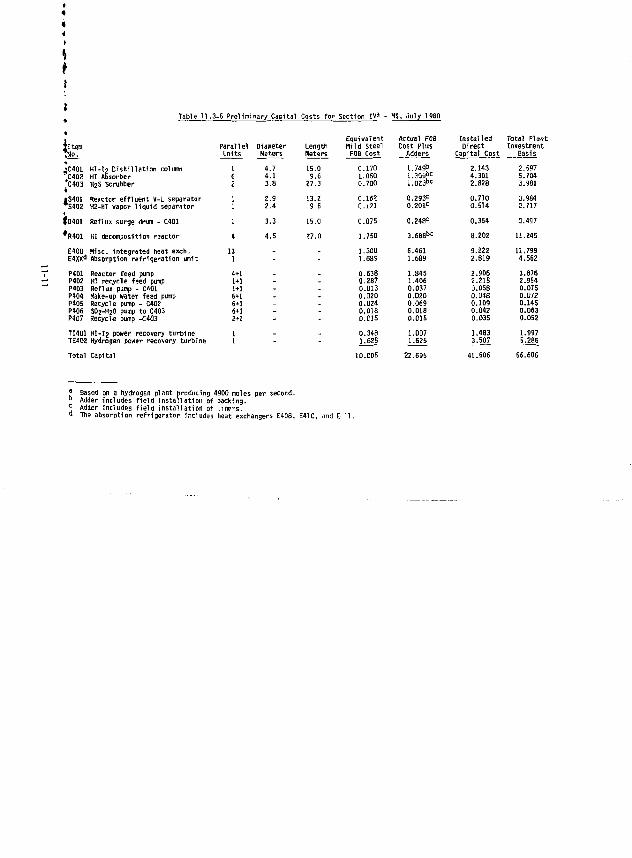
Table 11.3-5 Prel iminary Capital Costs for Section IV a - MS, Ju ly 19

Jltem %, -» ^C401 HI - I2 D i s t i l l a t i o n column " C402 HI Absorber "C4Q3 H2S Scrubber

*S40l Reactor e f f l u e n t V-L separator

S402 H2-HI vapor l i q u i d separator

fo401 Reflux surge drum - C401

R401 HI decomposition reactor

E400 Misc. in tegrated heat exch. E4XXd Absorption r e f r i g e r a t i o n un i t P401 Reactor feed pump P402 HI recycle fsed pump P403 Reflux pump - C401 P404 Make-up water feed pump P405 Recycle pump - C402 P406 SO2-H2O pump to C403 P407 Recycle pump -C403

TE401 HI - I2 power recovery tu rb ine TE402 Hydrogen power recovery tu rb ine

Total Capital

Parallel Units

Diameter Meters

Length Meters^

Equivalent Mild Steel FOB Cost

Actual FOB Cost Plus Adders

Installed Direct

Capital Cost

Total Plant Investment

Basis

4.7 4.1 3.8

15.0 9.6 27.3

0.170 1.050 0.700

1.749b l.S09°c

i.023bc

2.143 4.301 2.828

2.597 5.704 3.981

2.9 2.4

13.2 9 6

0.16? 0.121 0.201c

0.710 0.5U

0.984 0.717

3.3 15.0 C.075 0.248= 0.364 0.497

4.5 27.0 1.750 3.668bc 8.202 11.245

13 - - 1.300 1.689

6.461 1.689

9.222 2.819

11.799 4.562

4*1 1+1 !+l 6+1 6+1 6+1 2+1

: :

0.638 0.287 0.013 0.020 0.024 0.018 0.015

1.845 1.406 0.037 0.020 0.069 0.018 0.015

2.906 2.21S 3.058 0.048 0.109 0.042 0.035

3.876 2.954 0.075 0.072 0.145 0.063 0.052

1 1

- - 0.348 1.625

1.007 1.525

1.483 3.507

1.997 5.286

j * Based on a hydrog&n plant producing 4900 moles per second. D Adder includes f i e l d i n s t a l l a t i o n of packing. c Adder includes f i e l d i n s t a l l a t i o n of l i n p - s . u The absorpt ion re f r i ge ra to r includes heat exchangers E408, E41G, and E- "1T -

11.3.5 Power Systems Interface (Section Y)

The cost basis for Section V includes a l l of the helium coolant pumping, heat exchange, heat recovery, and shaft or electric power generation, except for the blanket heat exhangers (as covered 1n Section 11.3.6) and the process side (tube side) of the heat exchangers which are located within the Chemical Plant. We cost, in Section V, the shell side of al l of the in-process heat exchangers.

The results are shown in Table 11.3-6. The most significant costs are those for the helium gas turbine generator sets which are costed at $189/kWe

or $54.1O/kW^.f'0' This cost compares closely with those quoted by Pratt and Whitney Co.* 1 1 ) at $137.81/kWe ($49.34/kWt) f & r a n installed bare turbine generator set, and $174.61/kWe ($62.51/kWt> for installed units in a complete power station with land, buildings, accessory electric and power plant equipment and other minor expenses. Since we are not including land and power plant buildings, e tc . , the GA cost of $54.10/kWt appears a very reasonable compromise for our July 1980 dollar cost. Our application was discussed with Westinghouse(12) and Brown-Boveri'lS), and they confirm our choice of $54/kWt as a good estimate for July 1980 dollar costs.

The next most significant item is the steam generator. Using a quotation to GA by United Engineers and Constructors' 1 0), we take a value of $16.80/kWt in July 1980 dollars for a fabricated and installed steam generator unit including some indirect costs. Thus, a 2293M»t unit would cost $38.56M for the Heat Pipe Blanket, and a 1853 HWt unit would cost $31.13H for the Two-Zone Blanket.

Helium piping in both blanket designs is simple and inexpensive. We use a mild steel outer pipe which is from 100 to 200 K cooler than the helium. A 580 K stainless steel Inner l iner is perforated and spaced away from the cool,

11-12

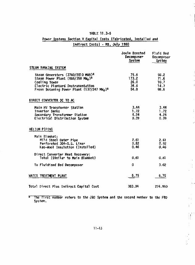
TABLE 11.3-6 Power Systems Section V Capital Costs (Fabricated, Installed and

Indirect Costs) - MS, July 1980

STEAM RANKINE SYSTEM Steam Generators (3780/2810 MWt)* Steam Power Plant (866/358 M W e ) a

Cooling Tower Electric Plantard Instrumentation Freon Botoming Power Plant (137/247 MWe)a

Joule Boosted Decomposer

System

75.6 173.2

26.0 34.6 54.8

Fluid Bed Decomposer

System

56.2 71.6 10.7 14.3 98.8

DIRECT CONVERTER DC TO AC

Main KV Transformer station Inverter Banks Secondary Transformer Station Electrical Distribution System

3.44 3.44 1.72 1.72 4.24 4.24 0.39 0.39

HELIUM PIPING

Main Blanket: Mild Steel Outer pipe Perforated 304-S.S. Liner Kao-Wool Insulation ( Instal led)

Direct Converter Heat Recovery: Total (Similar to Main Blanket)

To Fluidlzed Bed Decomposer

WATER TREATMENT PLANT

2.61 0.52 0.46

2.61 0.52 0.46

0.61 0.61

0 3.62

_S..75 5.75

Total Direct Plus Indirect Capital Cost 383.94 274.960

H The f i r s t number refers to the JBD System and the second number to the FBD System.

11-13

mild steel outer wall by 5 cm, and the space is insulated with Babcock and Wilcjx "Kao-Wool" spun mineral insulation.

A water treatment plant has been added to recondition the recirculated process water and to a minor extent precondition the make-up feed water. Water treatment consists of softening with ion-exchange and demineralization with reverse osmosis units, organic removal by carbon adsorption, and other •'.andard waste treatment operations. The plant is sized for a total recirculated water flowrate of 2.0 x 10^ moles H2O/S (8 million gallons per day), and costed at $5.00M.

11.3.6 Fusion-Driven Nuclear Island

For the Tandem Mirror Reactor, we have adopted the capital costs of W. Neff f 2) as indicated in Table 11.3-7, We applied a 1.5 factor to the two-zone blanket to account for the higher temperatures and additional complexity. We have not included any tubo-generator and electrical distibution equipment as part of the TMR costs, since they are included in Section V.

11.3.7 Summary of Capital Costs

Table 11.3-8 summarizes the capital costs developed above for the Thermochemical Plant and for the TOR Fusion Driver. The Thermochemical Plant estimates included the appropriate installation and indirect charges plus a contingency (usually 15%) to cover items not specified at this level of design e f for t . A 3% contactor's fee has been added, and a 52/y interest charge has been carried over a 3-year construction period which the amount of increases uniformly. We have assumed a 30-year chemical plant l i f e . Chemical plant costs have been scaled from the standard plant size of 4300 mole H2/sec to the actual size of 3942 mole H2/sec for the JBD plant and 5670 mole H2/sec for the FBD plant. We have added a 35% direct charge and contingency as expected for u t i l i t y Industr ies' 3 ' to construct the THR Fi1. on Driver. We have carried a

11-14

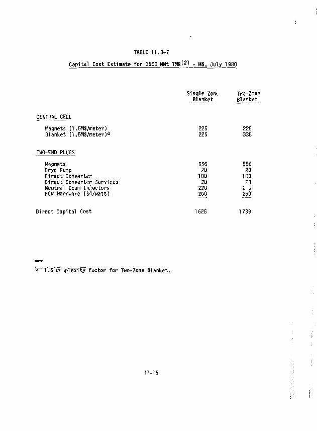
TABLE 11.3-7

Capital Cost Estimate for 3500 HWt TMR<2> - H$, July 1980

3 1.5 cr .p lexi ty factor for Two-Zone Blanket.

11-15

Single Zon*. Blanket

TVo-Zone Blanket

CENTRAL CELL Magnets (1,5M$/meter) Blanket {1.5M$/meter) a

225 225

225 338

TUO-END PLUGS Magnets Cryo Pump Direct Converter Direct Converter Services Neutral Beam Injectors ECR Hardware ($4/watt)

556 556 20 20

100 100 20 n

220 L J

260 260

Direct Capital Cost 1626 1739

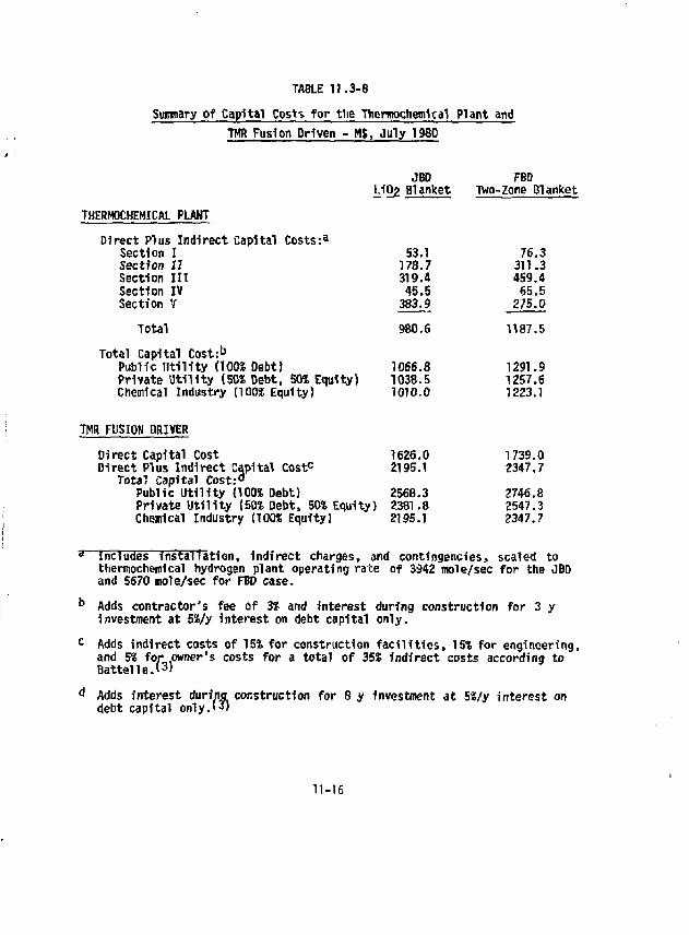
TABLE 11.3-8

Sumaary of Capital Costs for the Thermochemlcal Plant and TMR Fusion Driven - H$, July 1980

THERMOCHEMICAL PIAHT

Direct Plus Indirect Capital Costs:3

Section I Section I I Section l i t Section IV Section V

Total

Total Capital Cost:b

Public U t i l i t y (100S Debt) Private U t i l i t y (50$ Debt, 501 Equity) Chemical Industry (100S Equity)

JBD L102 Blanket

980.6

1066.8 1038.5 1010.0

FBD Two-zone Blanket

76.3 311.3 459.4 65.5

2/5.0

1187.5

1291.9 1257.6 1223.1

TMR FUSION DRIVER

Direct Capital Cost 1626.0 Direct Plus Indirect Capital Costc 2195.1

Total Capital Cost:" Public U t i l i t y (100% Debt) 2568.3 Private U t i l i t y (50% Debt, 50% Equity) 2381.8 Chemical Industry (100% Equity) 2195.1

1739.0 2347.7

2746.8 2547.3 2347.7

a Includes instal lat ion, indirect charges, and contingencies, scaled to thermochemical hydrogen plant operating rate of 3942 mole/sec for the JBD and 5670 mole/sec for FBD case.

0 Adds contractor's fee of 3% and interest during construction for 3 y investment at 5%/y Interest on debt capital only.

c Adds indirect costs of 15% for construction f a c i l i t i e s , 15% for engineering, and 5% for .owner's costs for a total of 35% indirect costs according to Battel le. 13)

Adds interest during construction for 8 y investment at 5%/y interest on debt capital only W

11-16

5$/y interest charge over an 8-year period where the amount of Investment increases uniformly over the period on the construction. These interest charges vary depending on whether the utility is public (100? debt) or private (50$ debt, 50S equity); and for the chemical industry, there is no interest charge since at IOCS equity the investment is carried by the chemical firm. We have assumed a 30-year fusion plant life as recommended by Battellet3'.

11.4 HYDROGEN PRODUCTION COSTS

11.4.1 Plant Availability

Vie assume the operating personnel of the Thermochemical Plant to consist of a day crew of three chemical engineers, one electrical engineer, five plant operators, one electronics technician, one computer systems-programmer, and one analytical process chemist; and four shift crews with 16 plant operators with the professional staff on call for four hour shifts or longer if required. Staffing of the TMR follows the guidelines set up by Battel!e for costing purposes.(3)

We have taken a 90% stream factor for the Chemical Plant, which takes into account 5% unscheduled and 5Z scheduled downtimes. We have assumed that owing to the process unit redundancies that we have designed into the Thermochemical Plant that plant failures can only reduce the stream factor to 80%. This results from the fact that there are at least 5 parallel process trains that are configured in a redundant fashion. One of the redundant trains could be shutdown 50% of the time, without reducing availability below the stated 90S level.

We hai/e taken a 77% TOR fusion plant availability as given by the Battelle report,^3' and assumed that this availability results from an IIS fraction of unscheduled shutdowns and \2% of scheduled shutdowns.

11-17

The combined overall system avai lab i l i ty , therefore, can be calculated from the above information as follows: The unscheduled avai labi l i ty is 1.00-0.11 or 0.8?, for the THR Driver and 1.00-0.05, or 0.95, for the Chemical Plant, producing a combined avai labi l i ty arising from random shutdowns as the product, which is 0.89 x 0.95 = 0,846. The scheduled fraction shutdown must be the larger of that for the THR Driver or the Chemical Plant; thus, 0.12 for the THR Driver. The total avai labi l i ty i s , therefore, the product of the scheduled avai labi l i ty times the unscheduled avai lab i l i ty , i .e . :

A = (1.00-0.12) x 0.846 = 0.744 (or 74.4S).

11.4.2 Estimates of Hydrogen Production Costs

The purpose of this section is to obtain the hydrogen production costs ($/GJ} from the estimated capital costs in Table 11.3.8, the chemical Plant operating costs in Table 11.4-1, and the Battelle methods*3' for the THR and electrical power systems. This will involve three different analyses: one based on public utility financing, one on private utility financing, and or° on chemical industry financing. Table 11.4-2 summarizes for the Heat Pipe Blanket the computation of H2 production costs utilizing the three different financing methods, while Table 11.4-3 summarizes the same information for the Two-Zone Blanket.

The computational procedure for both tables is identical. First, we need to separate the capital costs from Table 11.3-6 into the appropriate debt capital and equity capital portions depending upon how these capital cost expenditures are financed. Since the public utility is all debt financed either though prepayments of the rate payers under the justification of "future expansion" .or -under a utility-bond, the oapital costs are 100% debt financed. The private utility divides its capital between debt and equity capital [we assume 50% debt and 50% equity), while our model chemical industry takes it as entirely Internally (J003 equity) financed.

11-18

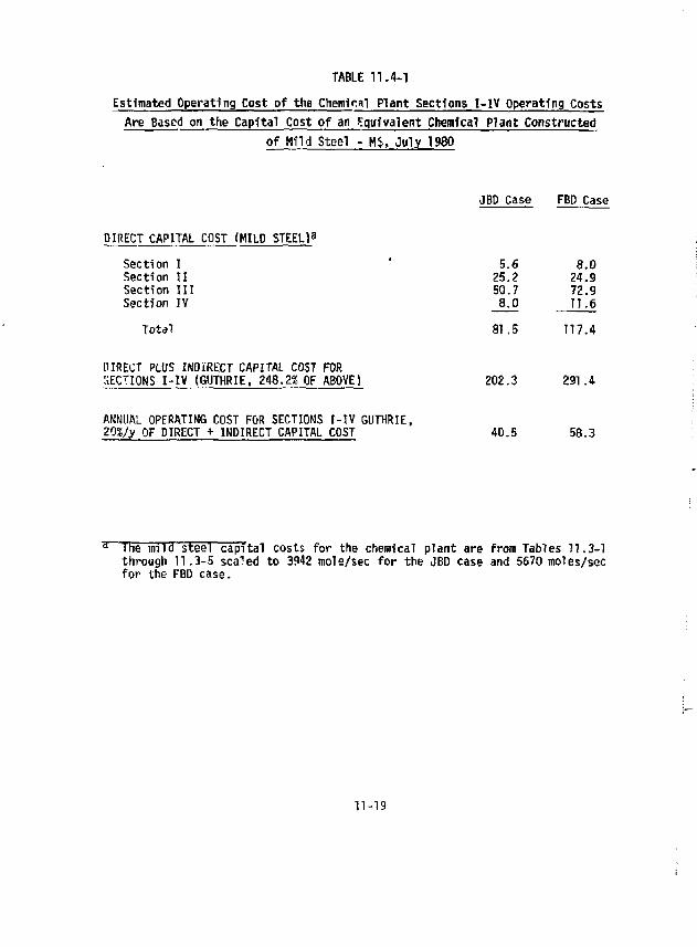
TABLE 11.4-1

Estimated Operating Cost of the Chemical Plant Sections I-IV Operating Costs Are Based on the Capital Cost of an Equivalent Chemfcal Plant Constructed

of Mild Steel - H$, July 1980

JBD Case FBP Case

DIRECT CAPITAL COST (HILD STEEL)3

Section I Section II Section III Section IV

Total 81.5 117.4

OIRECT PLUS INDIRECT CAPITAL COST TOR SECTIONS I-IV (GUTHRIE, 248.2% OF ABOVE) 202.3 291.4

ANNUAL OPERATING COST FOR SECTIONS I-IV GUTHRIE, 20%/y OF DIRECT + INDIRECT CAPITAL COST 40.5 58.3

5.6 8.0 25.2 24.9 50.7 72.9 8.0 11.6

I he mild steel capital costs for the chemical plant are from Tables 11.3-1 through 11.3-5 scaled to 3942 mole/sec for the JBD case and 5670 moles/sec fnr thp FRn ra«p for the FBD case.

n-19

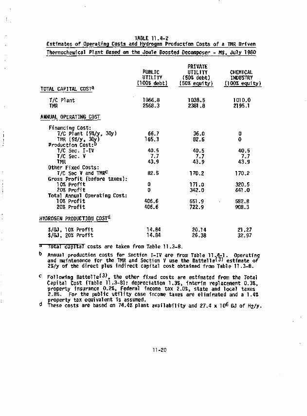
TABLE 11.4-2 Estimates of Operating Costs and Hydrogen Production Costs of a THR Driven Thermochemical Plant Based on the Joule Boosted Decomposer - Mt, July 1980

PRIVATE PUBLIC UTILITY CHEMICAL UTILITY (50% debt) INDUSTRY

(100% debt) (50* equity) (100* equity) TOTAL CAPITAL COST*

T/C Plant 1066.8 1038.5 1010.0 TMR 2568.3 2381.8 2195.1

ANNUAL OPERATING COST

Financing Cost: T/C Plant (5%/y, 30y) 66.7 36.0 0 THR (5$/y, 30y)

Production Cost: 0 165.3 82.6 0 THR (5$/y, 30y)

Production Cost: 0

T/C Sec. I - IV 40.5 40.5 40.5 T/C Sec. V 7.7 7.7 7.7 THR 43.9 43.9 43.9

Other Fixed Costs: T/C Sec V and TMRC 82.5 170.2 170.2

Gross Profit (before taxes): 10% Profit 0 171.0 320.5 202 Profit 0 342.0 641.0

Total Annual Operating Cost: 10? Profit 406.6 551.9 582.8 20% Profit 406.6 722.9 908.3

HYDROGEN PRODUCTION C0STd

$/GJ, 10% Profit $/GJ, 20% Profit

14.84 14.84

20.14 26.38

3 lotai capital costs are taken from Table 11.3-8.

21.27 32.97

Annual production costs for Section I-IV are from Table 11..4-1. Operating and maintenance for the THR and Section V use the B a t t e l l e ' 3 ' estimate of 2%/y of the direct plus indirect capital cost obtained from Table 11.3-8.

Following B a t t e l l e ' 3 ' , the other fixed costs are estimated from the Total Capital Cost (Table 11.3-8): depreciation 1.3%, interim replacement 0.3%, property Insurance 0.2%, Federal income tax 2.0%, state and local taxes 2.8%. For the public u t i l i t y case income taxes are eliminated and a 1.4% property tax equivalent Is assumed. These costs are based on 74.4% plant avai labi l i ty and 27.4 x 10 6 GJ of H2/y.

11-20

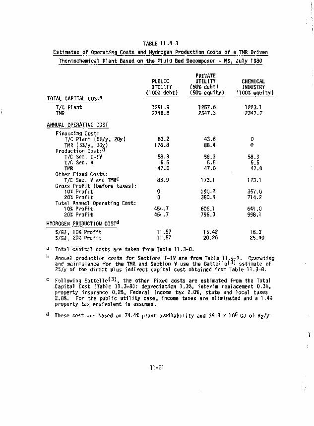
TABLE 11.4-3 Estimates of Operating Costs and Hydrogen Production Costs of a TMR Driven Thermochemical Plant Based on the Fluid Bed Decomposer - H$, July 1980

PRIVATE PUBLIC UTILITY CHEMICAL OTIL'.TY (50$ debt) INDUSTRY

(100% debt) (50% equity) '100% equity) TOTAL CAPITAL COST 3

T/C Plant TMR

ANNUAL OPERATING COST Financing Cost:

T/C Plant (5%/y, 20y) TMR (5%/y, 30y)

Production Cost:° T/C Sec. I-IV T/C Ssc. V TMR

Other Fixed Costs; T/C Sac. V and TMR C

fiross Profit (before taxi 10% Profit 20% P r o f i t

Total Annual Operating C< 10% P r o f i t 20% P r o f i t

HYDROGEN PRODUCTION C0STd

S/GJ, 10% P r o f i t $/GJ : 20% P r o f i t

H Total cap i ta l costs are taken from Table 11.3-8. b Annual production costs for Sections I - IV are from Table 11 .4 -1 . Operating

ant1 maintenance f o r the TMR and Section V use the B a t t e U e ' 3 ' estimate of 2%/y of the d i rec t plus i nd i rec t capi ta l cost obtained from Table 11.3-8.

c Following Battel l e ' 3 ' , the other f ixed costs are estimated from the Total Capital Cost (Table 11.3-8) : depreciat ion 1.3%, in te r im replacement 0.3%, property insurance 0.2%, Federal income tax 2.0%, state and local taxes 2.8%. For the publ ic u t i l i t y case, income taxes are el iminated and a 1.4% property tax equivalent is assumed.

d These cost are based on 74.4% plant a v a i l a b i l i t y and 39.3 x 70^ GJ of H2/y.

1291.9 2746.8

83.2 176.8

58.3 5.5

47.0

83.9

0 0

45'L7 45 ' . 7

11.57 11.57

1257.6 2547.3

43.6 88.4

58.3 5.5

47.0

173.1

190.2 380.4

606.1 796.3

15.42 20.26

1223.1 2347.7

0 0

58.3 5.5 47.0

173.1

357.0 714.2

641.0 998.1

16.3 25.40

11-21

V

This interest rate is based on constant dollars and is taken from the recommendations of the Battel!e report-^ 3 ' In an inflated economy as we have today the true interest rate is the 5%/y constant dollar interest rate over and above the current inf lat ion rate.

The annual production cost for the Chemical Plant (Sections I-Itf) i'j obtained directly from Table 11.4-1 based on a 20S fraction of the mild steel equivalent capital cost of the chemical plant. For the power systems (Section V) of the chemical plant and for the TMR, the mev^ds outlined by Ba t te l le ' 3 ' are followed as detailed in the footnotes to Tables 11.4-2 and 11.4-3. The gross prof i t is obtained as a simple percentage of the total equity capital .

From the above analyses, we can now obtain the hydrogen production cost. We use as our bissis a plant production rate of 3942 moles H2/sec for the JBD case and 5670 moles H2/sec for the FBD case. At a total combined avai labi l i ty of 74.4* (from Section 11.4-1) for the TMR/Thermochemical Plant, we obtain an energy production rate of ?7.4 ar.d 39.3 x 10 6 GJ/y for the two cases. This energy equivalence of the H? is obtained by using 285.77 kj/mol H2 as the higher heating value of H2 plus an added compressive value of energy of £T In P (9.70 kj/mol H2) associated with the 50 atm pressure of the hydrogen product, to obtain a total energy value of 295.47 KJ/mol H2. The hydrogen product cost in $/GJ is obtained by dividing the total annual operating costs (S/y? by the yearly hydrogen energy production rate (GJ/y).

11„5 CONCLUSIONS ON PRELIMINARY COST ESTIMATES

1 . Using conventional costing methods established by the fusion community and chemical industry, we obtain a hydrogen production cost of $12-15/GJ in July 1980 dollars for the FBD/Two-Zone Blanket approach and the JBD/Single-Zone Blanket concept assuming public u t i l i t y financing. Private u t i l i t y and chemial industry financing give higher costs.

11-22

2. The $12-15/GJ hydrogen cost obtained here is very favorable and indicates that fusion synfuels wi l l be competitive in the timeframe for emergence of fusion in approximately 2030.

11-23

References for Section 11.0

1 . M. S. Peters and K. D. Timmerhaus, "Plant Design and Economics for Chemical Engineers," McGraw-Hill, New York, 1980.

2. W. Neff, LLNL, private communication to R. W. Werner, September, 1982.

3. S. C. Schulte, T. L. Willke, and J . R. Young, Fusion Reactor Design Studies Standard Accounts for Cost Estimates, Pacific Northwest Laboratory, Battelle Memorial Inst i tute, Richland WA, Rept. PNL- 648 (May 1978).

4. R. H. Werner, et a l , "Conceptual Design Study FY 1981, Synfuels from Fusion-Using the Tandem Mirror Reactor and a Thermochemical Cycle to Produce Hydrogen," Lawrence Livermore National Laboratory Report UCID-19311.

5. K. M. Guthrie, "Capital Cost Estimating," Chemical Engineering 76, (6), 114-142 (1969).

6. K. M. Guthrie, "Capital and Operating Costs for 54 Chemical Processes," Chemical Engineering 77, (13), 140-156 (1970).

7. Marshall and Swift, Los Angeles, Equipment Cost Index, compiled quarterly, for 47 different industries reported regularly in Chemical Engineering, HcGraw H i l l , Mew York.

8. J . Smel!;o, Union Carbide Company, Cleveland, OH, private communication to T. Galloway of LLNL, June, 1981.

9. D. Stanwich, IngersoT Rand Company, Philipsburg, HA, private communication, August, 1982.

10. K. Schultz, Cost quotation for a 2240 MWt KTGR by United Engineers and Constructors Inc., private communication from . Schultz of General Atomic Company to T. Galloway of LLNL, March 2, 1981 .

11. Pratt * Whitney Co., "Advanced Nonthermally Polluting Gas Turbines and U t i l i t y Applications," U.S. EPA Report 16130 DNE 0371, March, 1971.

12. R. Foster-Pegg, Westinghouse Electric Company, private communication to T. Galloway of LLNL, July 30, 1981.

13. J . Parsoneault, Brown-Boveri Corp., St. Cloud, MN, and R. Davis Brown-Boverf Corp., Pasadena, CA, private communication to T. Galloway of LLNL, August, 1981.

11-24

SECTION 12 SYNFUELS BEYOND HYDROGEN

Contributor: R. G, Hickman

TABLE OF CONTENTS Section ZS3£ 12.0 SYNFUELS BEYOND HYDROGEN 12-1 12.1 METHANOL . . . . . 12-1

REFERFNCES 12-6

LIST OF FIGURES Figure Page 12.1 Reaction equilibrium constant Kp for CO + Zfy ZT~^ CH 3OH • • • 12-2 12.2 Equilibrium constants of chemical reactions . 12-4

i

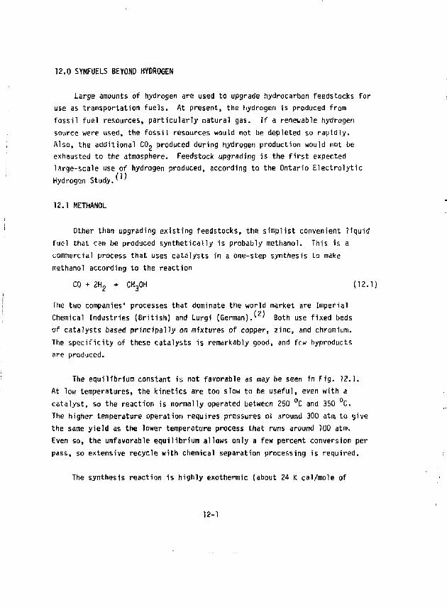
12.0 SYNFUELS BEYOND HYDROGEN

Large amounts of hydrogen are used to upgrade hydrocarbon feedstocks for use as transportation fuels. At present, the hydrogen is produced from fossil fuel resources, particularly natural gas. If a renei/able hydrogen source were used, the fossil resources would not be depleted so rapidly. Also, the additional CO, produced during hydrogen production would not be exhausted to the atmosphere. Feedstock upgrading is the first expected large-scale use of hydrogen produced, according to the Ontario Electrolytic Hydrogen Study.' '

12.1 METHANOL

Other than upgrading existing feedstocks, the simplist convenient liquid fuel that can be produced synthetically is probably methanol. This is a commercial process that uses catalysts in a one-step synthesis to make methanol according to the reaction

CO + 2H ? •+ CHgOH (12.1)

The two companies' processes that dominate the world market are Imperial Chemical Industries (British) and Lurgi (German). ' Both use fixed beds of catalysts based principally on mixtures of copper, zinc, and chromium. The specificity of these catalysts is remarkably good, and few byproducts are produced.

The equilibrium constant is not favorable as may be seen in Fig. 12.1. At low temperatures, the kinetics are too slow to be useful, even with a catalyst, so the reaction is normally operated between 250 °C and 350 °C. The higher temperature operation requires pressures of around 300 atm to give the same yield as the lower temperature process that runs around 100 atm. Even so, the unfavorable equilibrium allows only a few percent conversion per pass, so extensive recycle with chemical separation processing is required.

The synthesis reaction is highly exothermic (about 24 K cal/mole of

12-1

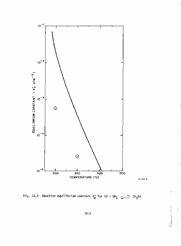
200 300 100 TEMPERATURE C O

500

F ig . 12.1 Reaction equ i l ib r ium constant K° fo r CO + 2H„ \.n* P 2 «= 3

CH,OH

12-2

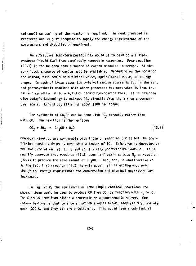
methanol) so cooling of the reactor is required. The heat produced is recovered and is just adequate to supply the energy requirements of the compressors and distillation equipment.

An attractive long-term possibility would be to develop a fusion-produced liquid fuel from completely renewable resources* From reaction (12.1) it can be seen that a source of carbon monoxide is needed. At the very least a source of carbon must be available. Depending on the location and demand, this could be municipal waste, agricultural waste, or energy crops. In each of these cases the original carbon source is C0 ? in the air, and photosynthesis combined with other processes has separated it from the air and converted it to a solid or liquid hydrocarbon form. It is possible with today's technology to extract C0 2 directly from the air on a commer­cial scale. Liquid CCL, sells for about ?100 per tonne.

The synthesis of CH-,0H can be done with CO- directly rather than with CO. The reaction is then written

C0 Z + 3H 2 + CH 30H + H 20 (12.2)

Chemical kinetics are comparable with those of reaction (12.1) but the equi­librium constant drops by more than a factor of 10. This drop is depicter. by the two circles on Fig. 12.1, and it is a very unattractive feature. It is readily observed that reaction (12.2) uses half again as much H 2 as reaction (12.1) to produce the same amount of CH,0H. That, too, is unattractive as is the fact that reaction (12.2) is only about half as exothermic, even though the energy requirements for compression and chemical separation are increased.

In Fig. 12.2, the equilibria of some simple chemical reactions are shown. Some could be used to produce CO from C0 2 by reacting with H 2 or C. The C could come from either a renewable or a nonrenewable source. One common feature is that to show a favorable equilibrium, they all must operate near 1000 K, and they all are endothermic. This would have a substantial

12-3

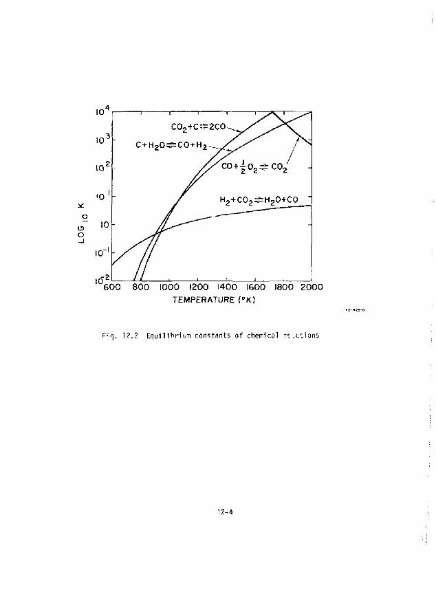
C O o + C ^ C O -

C + H 2 0 ^ = C O + H 2 .

c o + | o 2 ^ c o 2

H 2 + C 0 2 ^ H 2 0 + C 0

600 800 1000 1200 1400 1600 1800 2000 TEMPERATURE (°K)

Fig. 12.2 Equilibrium constants of chemical reactions

12-4

influence on the f ina? methanol cost. A reaction lot shown but worthy of consideration is the partial oxidation of biomass char with surplus oxygen produced during hydrogen manufacturing. This oxidation is exothermic and the heat at the reaction temperature could produce the char in a conventional pyrolysis step. Regardless of the final choices made, many routes to synthetic liquid fuels are available once the H^ can be produced in abun­dance at low enough costs.

A closing comment might tie made here. With a two-step catalytic dehy­dration process known as Mobil M, methanol can be converted to high octane gasoline at about 90% efficisncy.

12-5

References for Section 12.0

1. "Hydrogen, A Challenging Opportunity," Report of the Ontario Hydrogen Energy Task Force, Vol. 1, September 1981.

?. R. Salmon, M. Edwards, and R. Wham, "Production of Methanol and Methanol Related Fuels from Coal," Oak Ridge National Laboratory, Rpt, 0RNL-5564.

12-6

SECTION 13 SIMULATION OF SECTION II OF GENERAL ATOMIC THERMOCHEMICAL CYCLE

AND THE THERMODYNAMICS OF THE HgSO^-HgO SYSTEM Contributors:

M. E. Abhold, J. Oelund and A. L. Babb

TABLE OF CONTENTS Section Page 13.0 SIMULATION OF SECTION II OF GENERAL ATOMIC THERMOCHEMICAL

CYCLE AND THE THERMODYNAMICS OF THE H 2S0 4-H 2G SYSTEM 13-1 13.1 CHESS: The U.W. Process Simulation Code 13-1

13.1.1 Description of CHESS 13-1 n.1.2 Modifications to CHESS for Electrolyte Systems 13-4 13-1.3 Example Add-On Module for the Multi-Effect

H S0 4 Evaporators 13-4 13.2 Review of Relevant Data and its Deficiencies 13-8 13.3 References 13-16

i

SECTION 13 List of Figures

Figure Page

13.1-1 CHESS Input Schematic fo r Section I ] 13-5

13.1-2 Isothermal Flash Module 13-6

13.2-1 Total Pressures above Aqueous Su l fu r i c Acid 13-11

13.2-2 Boi l ing and Condensation Points above Aqueous Su l fu r ic Acid 13-12

13.2-3 Comparison of Calculated wi th Measured Azjotrope f o r Aqueous Su l fu r ic Acid 13-13

13.2-4 Comparison of Calculated wi th Measured Pressures above

Aqueous Su l fu r i c Acid 13-13

13.2-5 Total Pressure fo r Aq. H-SO^ at Azeotrope 13-14

13.2-6 Par t ia l Pressure for H„0 over Aq. HjSCL, at Azeotrope.. . 13-14

13,2-7 Par t ia l Pressure of H-SO. over Aq. HjSQ. at Azeotrope.. 13-15

13.2-8 Par t ia l Pressure of S0„ over Aq. H-SCL at Azeotrope 13-15

L i s t of Tables / Table Page

13.2-1 SO, Enthalpy Data 13-8

n

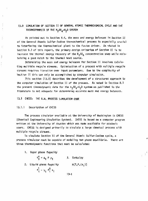
13.0 SIMULATION OF SECTION II OF GENERAL ATOMIC THERMOCHEMICAL CYCLE AND THE THERMODYNAMICS OF THE HgSO^HgO SYSTEM

As pointed out in Section 9.4, the mass and energy balances in Section II of the General Atomic Sulfur-Iodine thermochemical process is especially crucial to interfacing the thermochemical plant to the fusion driver. As stated in Section 9.3 of this report, the primary design criterion of Section II is to increase the thermal energy recovery of the HjSO^ concentration step while main­taining a good match to the thermal heat source.

Determining the mass and energy balances for Section II involves calula-ting multiple recycle streams. Optimization of a process with multiple recycle streams requires iteration over input parameters. Due to the complexity of Section II this can only be accomplished by computer simulation.

This section (13.0) describes the development of a structured approach to the computer simulation of Section II of the process. As noted in Section 8.1 the present thermodynamic data for the H-SO^-H-O system as published in the literature is not adequate for determining accurate mass and energy balances.

13.1 CHESS: THE U.W. PROCESS SIMULATION CODE

13.1.1 Description of CHESS

The process simulator available at the University of Washington is CHESS (Chemical Engineering Simulation System). CHESS is based on a computer program written at the University of Houston which was made available for academic users. CHESS is designed primarily to simulate a large chemical process with multiple recycle streams.

To simulate Section II of the General Atomic Sulfur-Iodine cycle, a process simulator must be capable of modeling two phase equilibria. There are three thermodynamic functions that must be calculated:

3. Enthalpy

H(T,P,{x.})

13-1

1. Vapor phase fugacity f i - *i P *1

2. Liquid phase fugacity

' i - 1 , < ; « ,

where:

$. = fugacity coefficient

P = total pressure

•Hi y. = mole fraction of i species in the vapor phase

Y- = activity coefficient

f. = fupacity of the pure liquid at it's vapor pressure for that temperature

x. = mole fraction of the i species in the liquid phase

H = total enthalpy

The prediction method used by CHESS for enthalpy and fugacity coefficients is the Redlich-Kwong-Suave equation of state. This method was chosen because of the ability to select the constants appearing in the equation with a minimum of data (critical pressure, critical temperature, and an accentric factor for each chemical species). Because of it's simplicity, the Redlich-Kwong equation could not be expected to be sufficiently accurate to be used in precision calculations. It has, however, been used frequently for mixture calculations and pi tse equilibrium correlations with reasonably good success,

le liquid activity coefficient is much mors difficult to determine since it defends on liquid-liquid interactions which vary greatly depending on whether the molecules are polar, electrolytic, or neither. The simplest situation is an ideal solution where the activity coefficients are one. The next most complicated, is the regular solution theory used by CHESS. The regular solution theory applies to solutions whose excess entropy of mixing is zero. This approach is suitable for non-polar of very weakly polar compounds. The liquid phase fugacity is based upon an empirical curve which includes a correction for the Pitzer-Curl acentric factor. Liquid activity coefficients are based on the

13-2

Hildebrand solubility parameter method with coefficients provided by Chao and Seader.

The CHESS system requires that the user supply information on (1) the feed streams to the process, (2} the process topology, and (3) designation of the type of process equipment and its parameters (i.e. a heat exchanger, number of shells, area, heat transfer coefficient etc.). CHESS then completes the mass and energy balanu^s and provides a summary of (1) each stream, vapor fraction, temperature, pressure, enthalpy, and composition, and (2) each process unit: cooling required, work required. Although CHESS has some capability for design it is primarily suited for simulation.

The process units included in CHESS offer the capability of doing the following kinds of calculations (all multicomponent):

Absorber/Stripper — separation using several theoretical stages Flash — isothermal or adiabatic Distillation — plate to plate

— short cut Heat exchangers Reactor — calculates stoichiometry only, no

equilibrium constraints Pumps Valves Fired Heators

The restrictions on the system are:

(1) < 100 streams (2) £ 50 pieces of equipment (3) £ 20 components (4) regular liquid solutions (5) ideal vapor solutions (i.e. vapor activity coefficients are one)

13-3

13.1.2 Modifications to CHESS for Electrolyte Systems

In or<Jer to simulate Section II of the General Atomic Sulfur-Iodine cycle, CHESS must be able to predict the vapor phase fugacity, liquid phase fugacity, and enthalpy for the H^SO^ • H,0 • S0 3 system. The prediction methods used by CHESS assume regular solutions and therefore are incapable of accurate predictions for the components in question.

It i; necessary to add unit computation modules to CHESS to model the vapor liquid equilibrium of HySO. • H ?0. The modules will utilize the thermodynamic data discussed in Section 13.2 empirically.

The CHESS input Schematic for Section II is shown in Fig. 13.1-1. As the Redlich-Kwong-Soave equation of state is adequate to predict vapor phase enthalpys, the standard CHESS unit calculation modules will be used in the vapor phase. For units which calculate vapor-liquid equilibrium modules will be added.

13.1.3 Example Add-On Module for the Multi-Effect H,S0. Evaporators

The ADD1 module is an additional module added to the CHESS program to carry out isothermal flashes. Fig. 13.1-2 shows a schematic of the ADD! module. With the equilibrium data discussed in Section 13.1, the ADD1 module will solve an isothermal flash with known K-values.

13-4

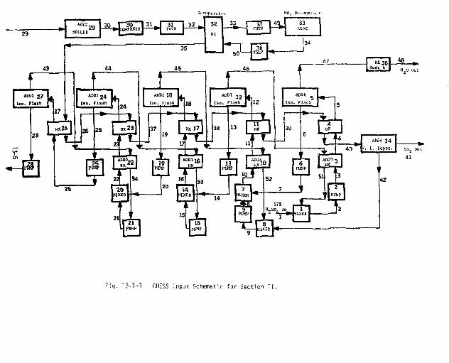
5 0 ' — | V * L V J "

SOj Ut-v tntipc.s

3 3 KEAC

Iso. Flash

AUDA 3 4

40 ~" fr. L. Separ

t-iq. 13-1-1 CHESS '.nput Schematic for Section II.

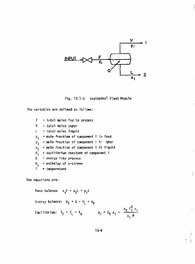
V

T

yr

* ™ - { > 0 £, •( , ••)

Fig. 13.1-2 Isothermal Flash Module

The variables are defined as follows:

= total moles fed to process = total moles vapor = total moles liquid = mole fraction of component i In feed = mole fraction of component i 1r apor = mole fraction of component i in liquid = equilibrium constant of component i = energy into process = enthalpy of x-stream = temperature

The equations are:

Mass balance: z.F = x A + y-V

Energy balance: H f + Q = H. + R,

Equilibrium; T p = T L = Ty yi = *S xi xi f i Ti

13-6

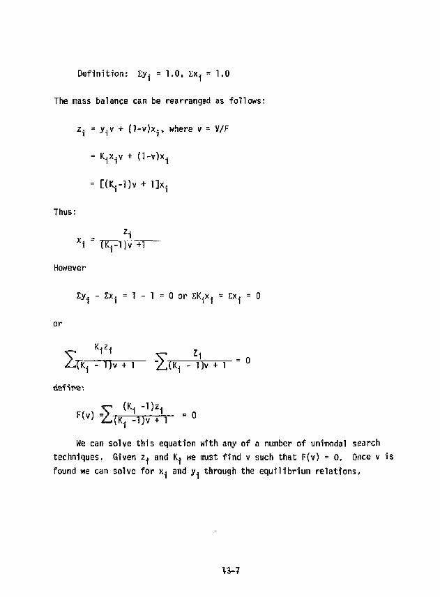
Definition: Ey^ = 1.0, Ex i = 1.0

The mass balance can be rearranged as follows:

*i - y^v + (l-v)x., where v = V/F

= K^.v + (l-v)xi

= C(K rl)v + l ] X i

Thus: zi

However

Zy* - Ex. = 1 - 1 = 0 or EK.x. = Ex. = 0

or K.Z t

Y v zi Z,"^ - 1 )v + 1 "ZlK-j - l)v + 1 " °

F< V> =Z,(K- -1)v A = ° defif-e'.

^K H - 1 ) Z |

Ci We can solve this equation with any of a number of unimodal search

techniques. Given z. and K. we must find v such that F(v) = 0. Once v is found we can solve for x. and y, through the equilibrium relations,

13-7

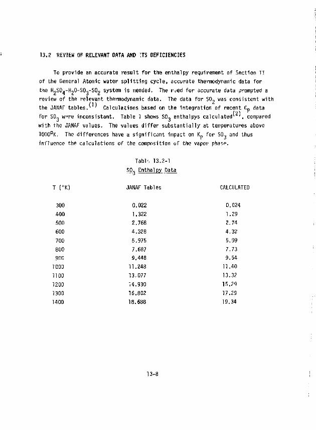
13.2 REVIEW OF RELEVANT DATA AND !TS DEFICIENCIES

To provide an accurate result for the enthalpy requirement of Section II of the General Atomic water splitting cycle, accurate thermodynamic data for the HpSOj-hUO-SOg-SOp system is needed. The r-jed for accurate data prompted a review of the relevant thermodynamic data. The data for SO, was consistent with the JANAF tables/ ' Calculations based on the integration of recent C p data for SO, w^re inconsistant. Table 1 shows SO., enthalpys calculated^ , compared with the JANAF values. The values differ substantially at temperatures above 1000°K. The differences have a significant impact on K p for SO, and thus influence the calculations of the composition of the vapor phase.

Tabl'; 13.2-1 SO, Enthalpy Data

T (°K) JANAF Tables CALCULATED

300 0.022 0.024 400 1.322 1.29 500 2.768 2.74 600 4.328 4.32 700 5.975 5.99 800 7.687 7.73 9DD 9.448 9.54 1000 11.248 11.40 1100 13.077 13.32 1200 14,930 15.29 1300 16.802 17.29 1400 18.688 19.34

13-8

Also of importance for separations operations are data on the vapor liquid equilibrium of the HpO-H^SO* system, over the complete range of concentrations and at elevated temperatures. To date the best estimation of the properties of aqueous sulfuric acid have been made by Gmitro and Vermeulerr ' They used an iterative procedure, normalizing to the azeotrope, to calculate the partial pressures over sulfuric acid over the complete range of dilution and up to temperatures of 400° C. Their calculations were essentially extrapolations of room temperature data, the estimate of the properties of aqueous sulfuric acid not being of sufficient reliability for the calculation of separations operations at high temperatures,

Excellent measurements of the vapor-liquid equilibrium of aqueous sulfuric acid have recently been made by Lennartz^ ' They include joth P-T-x and T-x-y data. The P-T-x measurements span the range of concentrations from 20-100% mole fraction hz$0„, with a temperature range of 110-500°C. The results are shown in Fig. 13.2-1. The T-x-y measurements also covered a wide range and are shown in Fig. 13,£-2. The azeotrope was determined from both P-T-x and T-x-y measurements and is shown in Fig. 13.2-3.

Currently, no analysis of Lennart-s' data has been published. Nonetheless, rough comparison between Gmitros' calculations and Lennartzs' data can be made using the data as presented in figs. 13.2-1 to 13.2-3.

The comparison between total pressures as measured by Lennartz and calculated by Gmitro is shown in Fig, 13.2-4. The largest discrepancy in total pressures lies in the region near the azeotrope. Calculations made at the azeotrope as measured by Lennartz show that this is due to significant errors in the partial pressures of SO, and H 2S0.. These errors have a significant impact on the distribution coefficients between the liquid and gaseous phases at equilibrium. The discrepancy is demonstrated by comparison of the partial pressures at the azeotrope as shown in Figs. 13.2-5 to 13.2-8. (At the azeotrope the partial pressures above the solution can easily be found with the published data.) While such a limited comparison cannot indicate the extent of error over the whole range of solutions, it shows that there are points at which the discrepancy is on the order of 100% for both SO, and H,S0.. Again, the implication 1s that the distribution coefficients are off by a significant amount. Also note that the total pressure temperature dependence is significantly different from that measured at the azeotrope

13-9

(see Fig. 13.2-4). This implies a large percentage error in the enthalpy of -porization near the azeotrope.

Note that (see Fig. 13.2-6) the difference between the partial pressures for H„0 is minor in relation to the errors in the partial pressures of S0 3 and H„S(L (Figs, 13.2-7 and 13.2-8). This explains the excellent agreement between th= two sets of total pressure data at lower mole fractions of H2S(L where the partial pressures of H,SO. and SO, are negligible (see Fig, 13.2-4). Th'js the error in Gmitros' calculations is almost solely due to errors in the partial pressures of H 2S0 4 and SC,.

In view of the fact that the efficiency of the entire synfuel plant is strongly impacted by the efficiency of the separations operations the current thermochemical data being used for engineering analysis is inadequate for process optimization. In light of this situation the measurements made by Lennartz are currently being reduced to provide the relevant thermodynamic data for the hLO-HpSO, system.

13-10

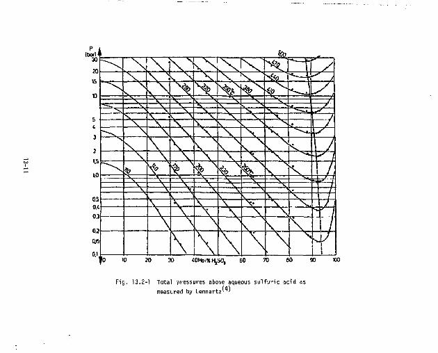
<OMol%H,SO,. 50 90 «0

Fig. 13.2-1 Total pressures above aqueous sulfuric acid as measured by Lennartz^ '

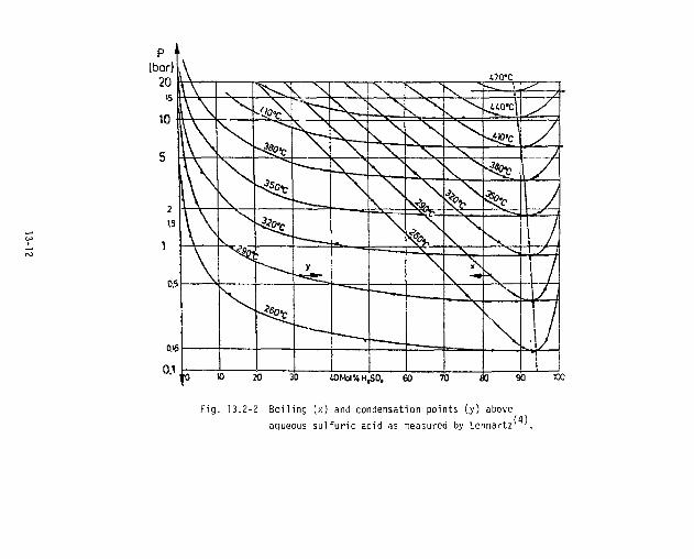
t?o°c

80 90 SO

Fig. 13.2-2 Boiling (x) and condensation points (y) above (4) aqueous sulfuric acid as measured by Lennartz1 '.

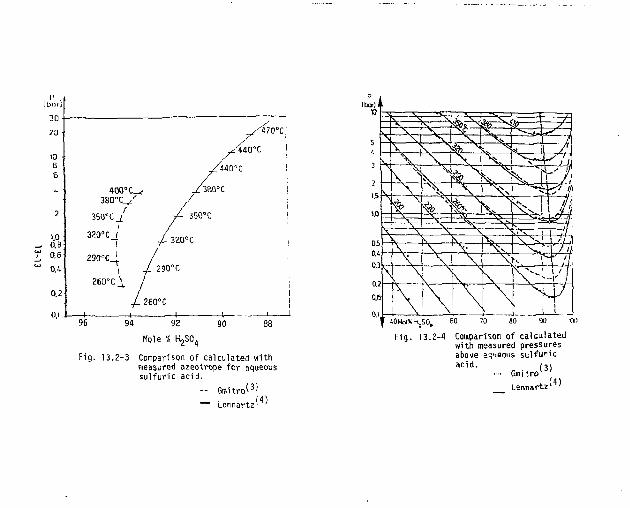
Ibm)

Fig. 13.2-3 Comparison of calculated with measured azeotrope for aqueous sulfuric acid.

-- Gmitro'3' II) — Lennartz'

' J tOMol'KHjSO,. Fig. 13.2-1 Comparison of calculated

with measured pressures above aqueous sulfuric acid. ,3) •••• Gmitro* '

Lennartz (4)

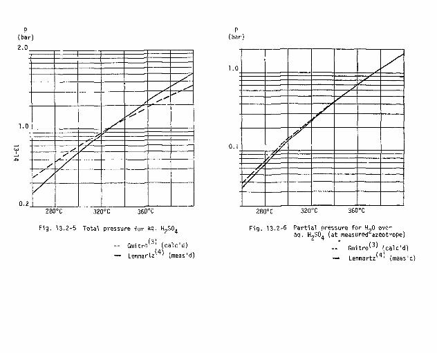
p (bar) 2.0

1.0.

0.2.

/ / r ^

^ • " **

r *->' ,<f

y s /

/

p (bar)

1.0

0.1 1

.•/ >/ / ' // 7

280°C 320°C 360°C 280°C 320°C 360°C

Fig. 13.2-5 Total pressure for aq. HjSO^

- Gmi t ro ( 3 > (calc 'd) — Lennartz^ ' (meas'd)

Fig. 13.2'6 Partial pressure for HoO over aq. H„S0. (at measured azeotrope)

— Gmitro'3' (calc'd) —- Lennartz (meas'd)

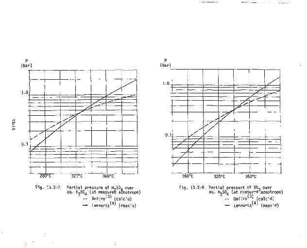
p (bar)

1.0

0.1

-, . -, . /' / ~.— s^-*

s K

280°C 320°C 360°C

Fig. i'i.1-1 Partial pressure of H,S0i over sur

— Gmitro'3'

rartiai picssuic 01 n~ou* uver aq. HJJSG^J (at measures azeotrope)

(calc'd) — Lennartz' ' (meas'ri)

P (bar)

.0 /

-— / > ' x ---/> "" ^

S *7

yy i

n.i •^ 7* s

/ ^ / / 1 / V \

280°C 320,>C 360°C

Fig. 13.2-8 Partial pressure of SO, over aq. H,S0. (at measured azeotrope)

-- Gmitro'3' (calc'd) — Lennartz' ' (meas'd)

REFERENCES

1. D. R. S tu l l and H. Prophet, "OANAF Thermodynamic Tables", 2nd e d . , U.S. National Bureau of Standards, (1971), Washington D.C., w i th Supplements through March 3 1 , 1979.

2. C. L. Yaws, K. Y. L i , C. H. Kvo, "Sulfur Oxides SO,, SO,", Chem. Eng. July 8, 1974 pp. 87. L 6

3. 0 . 1 . Ganitro, and T. Vemeulen, T. , "Vapor-Liquid Equilibria for Aqiieous Sulfuric Acid", University of California, Ernest 0. Lawrence Ftadiafon Laboratory, Berkeley, Cft, Report No. UCRL-10886, June 24, 1963.

4. A. A. Strub .;nd G. Imar is io , Eds., I n : Proc. I n t . Seminar, "Hydrogen as an Energy Vector", Brussels, Belgium, February 1980. Published by Durdrecht, Holland, 1980.

GPO 687 -jaz/P90dl 13-16