SP

RI

NG

2

00

8

V O L 2 5 I S S U E 0 1

S p a c e T e l e s c o p e S c i e n c e I n s t i t u t e

The Last Confessions of a Dying Star Image Credit: NASA, ESA, and the Hubble Heritage Team (STScI/AURA) http://hubblesite.org/newscenter/archive/releases/2008/13/

M. Stiavelli, mstiavel@stsci.edu, and H.S. Stockman

Synergy Between Webb and Hubble

Hubble will have restored and enhanced science capabilities after Servicing Mission 4 (SM4), planned for late summer 2008. Current SM4 plans call for the repair of the Space Telescope Imaging Spectrograph (STIS) and the Advanced Camera for Surveys (ACS), and the installation of two new instruments: Wide Field Camera 3 (WFC3) and the Cosmic

Origins Spectrograph (COS). WFC3 will offer a significantly wider field in the near infrared than the Near Infrared Camera and Multi-Object Spectrometer (NICMOS), and COS will be more sensitive in the ultraviolet than STIS. These instrument changes and the other Hubble repairs will sustain key observatory capabilities for the next five years, up to the planned launch of the James Webb Space Telescope. Nevertheless, even though the Hubble and Webb science missions may overlap, astronomers would be wise to assume that the overlap will be brief, and they should consider the implications for Webb science programs.

The Webb telescope is optimized for operations in the near- and mid-infrared, and for imaging and low- to medium-resolution spectroscopy. Its nominal wavelength range is between 1 and 28 microns. The telescope is diffraction limited at wavelengths longer than 2 microns. Webb instruments are capable of taking high-angular resolution images and low-

resolution spectra down to the V band, but the performance below 1.6 micron is not guaranteed by specific mission requirements. Nevertheless, we expect Webb to be significantly more sensitive than Hubble in the overlapping wavelengths between 0.6 and 1.7 microns. Webb is capable of multi-object spectroscopy at spectral resolving powers up to 3000. Webb also has a complement of coronagraphs for high-contrast imaging. Meanwhile, Hubble will remain unique amongst space observatories for visible and ultraviolet imaging (WFC3/ACS) and spectroscopy (COS/STIS). Hence, most Webb science will not repeat Hubble science, but extend and complement it in the infrared.

What Hubble data might be needed to enable Webb science for broad science areas?

High-redshift galaxies

Webb will identify candidates for high-redshift galaxies using broad-band filters to identify spectral features due to the Lyman break and Lyman-alpha forest. Unfortunately, this technique is subject to false detections of low-redshift interlopers (e.g., a Balmer break at low redshift). Deep visible imaging down to the B band and perhaps into the ultraviolet can

Continuedpage 2

2

rule out such interlopers, but these wavelengths are not accessible to Webb. Therefore, Webb searches for high-redshift galaxies must take place in areas of the sky where Hubble data are already available. (Ground-based surveys cannot reach the necessary deep magnitudes, AB ~ 30–31.) Several deep Hubble fields already exist, and these will be prime candidate fields for deep Webb observations. They may be sufficient, but they entail two potential issues. First, we expect galaxies at high redshift ( z > 7) to be rare, but we have yet to learn how rare. The problem of eliminating low-redshift interlopers becomes more important if the likely number of bona fide sources is small. Similarly, it may be necessary to have larger fields than the Hubble visible and B-band images currently available. Second, Webb searches for high-redshift supernovas could be most efficient in the continuous viewing zones (CVZs), which can be observed at all times. The Webb CVZs lie within 5 degrees of the ecliptic poles. The most important area for extragalactic applications is the northern CVZ, which does not contain any of Hubble deep extragalactic fields. Thus, unless additional Hubble data are taken in the northern CVZ, the deep fields from Webb that come as byproducts of supernova searches will not be fully useful for high-redshift galaxy studies. To ensure a foundation for Webb high-redshift galaxy and cosmology programs by resolving these issues would require additional Hubble observations.

Nearby galaxies

A complete census of nearby galaxies of all major morphological types requires observing galaxies up to distances of 10–20 Mpc. Unfortunately, Hubble data are complete only for objects within approximately 4 Mpc. At larger distances, Hubble has observed many galaxies, but the data set is mixed with respect to filters, exposure times, and selection criteria. Most of the existing

data on nearby galaxies were obtained in snapshot surveys, with limited available ultraviolet or B-band data. Unfortunately, some of the standard filters combinations used to disentangle age, metallicity, and dust content also require imaging at wavelengths below the V band. Thus, unless alternative diagnostics are developed in the infrared, astronomers will need Hubble data in these bands to support detailed study by Webb. An alternative diagnostic approach could be to rely more extensively on spectroscopy by exploiting the multi-object capabilities of Webb. The study of objects in the Local Group that can be resolved into stars faces similar difficulties, as many of the existing deep fields do not include ultraviolet or B-band images. The Large Magellanic Cloud lies largely within the Webb southern CVZ, and it is likely to be the object of detailed population studies. Once again, any required ultraviolet or B-band images should be obtained beforehand with Hubble.

Galactic objects

Many datasets exist in the Hubble archive for a wide assortment of galactic objects, such as planetary nebulae, supernova remnants, globular clusters, and star-forming regions. For studies requiring narrow-band images to examine specific emission lines, it may be necessary to substitute near-infrared lines for the usual visible lines, since the set of visible, narrow-band filters available to

Synergy from page 1

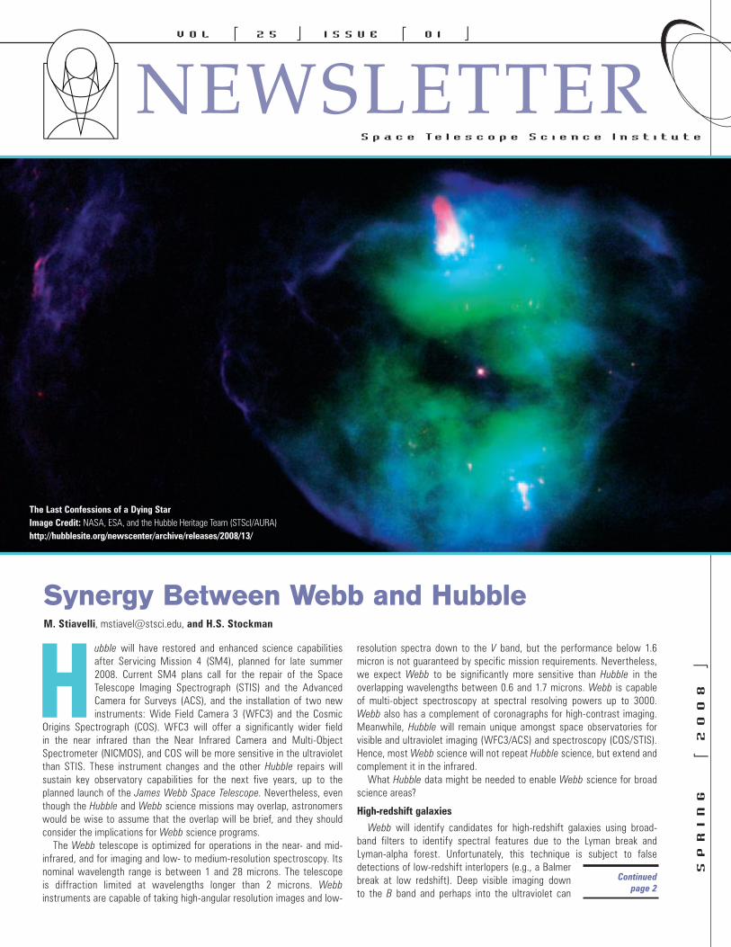
Figure 1. Comparison of the angular resolution of Hubble and Webb in the near infrared. The left image has been obtained with Hubble’s Near Infrared Camera and Multi-Object Spectrometer as part of the Hubble Treasury program on the Ultra Deep Field (PI: R. Thompson). The right image is a simulation of the same field as seen by Webb. The image was produced by deconvolving the NICMOS image using 40 iterations of the Richardson-Lucy algorithm and then convolving it with the expected Webb point-spread function. The spectral bands are F110W and F160W for NICMOS and F110W and F150W for Webb’s Near Infrared Camera.

3

ACS Report R. Gilliland, gillil@stsci.edu

The Advanced Camera for Surveys (ACS) continues to operate with the solar blind channel (SBC) receiving some 12% of the Cycle 16 observing time on Hubble. ACS repair (ACS-R) of the wide-field camera (WFC) and the high-resolution camera (HRC) are planned for Servicing Mission 4 later this year. The ACS-R development is proceeding well and is on track. The ACS team has successfully demonstrated that the ACS-R design can deliver

the expected performance from the charge coupled devices (CCDs), and is integrating and testing a fully flight-representative engineering model. Fabrication of the flight hardware has started. In parallel, team members are working on the hardware carrier, software, operational aspects, and planning tests and extra-vehicular activities, among other areas critical to ACS-R success. So far, so good!

Preparations for the Servicing Mission Orbital Verification (SMOV) period for the repaired ACS are well underway. Calibration programs executed as part of SMOV for the ACS will establish the basic characteristics of the instrument on orbit. In conjunction with early calibrations in Cycle 17, we expect to restore knowledge of instrument characteristics—like readout noise, flat fields, sensitivity, and charge transfer efficiency (CTE)—and calibrations to a level comparable to that before loss of the CCD-based channels of the ACS on January 27, 2007. We expect to fully support Cycle 17 science observations with the ACS.

A large number of characterization and calibration activities have been completed since the previous Newsletter article and detailed in corresponding instrument science reports (ISRs). M. Chiaberge and M. Sirianni provided updated measurements of red leaks for ultraviolet and narrow-band filters for the ACS CCDs (ACS ISR 07-03). V. Kozhurina-Platais, P. Goudfrooij, and T. Puzia discussed differential CTE corrections for both photometry and astrometry for non-drizzled WFC images in ACS ISR 07-04. A contribution from the community by K. Collins et al. (ACS ISR 07-05) reported the detection and characteristics of a new ghost in F122M used with the SBC. R. Bohlin provided a new absolute photometric calibration of the ACS CCD cameras in ACS ISR 07-06 based on observations of spectrophotometric standard stars and comparison to synthetic photometry. In a program anticipating Webb astrometric calibration needs, R. van der Marel et al. (ACS ISR 07-07) refined the absolute WFC scale and rotation. In ACS ISR 07-08, J. Anderson established small temporal changes in the linear skew terms of the WFC since its installation in 2002, and incorporation of this effect in pipeline processing is under way. J. Maíz Appellániz described preparatory work (ACS ISR 07-09) establishing astrometric fields in NGC 604 and NGC 6681, which

Webb is quite limited. As for all other areas of science, availability of blue or shorter wavelengths might become a limiting factor for some Webb science projects, unless those data are obtained by Hubble. Webb also lacks the astrometric and polarimetric capabilities of Hubble, and Webb observations requiring such data must rely on prior Hubble observations.

QSO absorption systems

Due to its limited spectral resolution, Webb is incapable of studying in detail the Lyman-alpha forest and the metal absorbers seen in the spectra of QSOs. However, the systematic study of feedback and the interplay between gas and stars in galaxies requires a statistical study of galaxies in fields where QSO spectra have been measured. Hubble provides unique data on QSO absorption systems at z < 3. Webb will be capable of studying the properties of the galaxies associated with those absorbers. The combination of these complementary measurements by Hubble and Webb will provide essential constraints to study how the IGM is enriched by galaxies.

In summary, Webb science will rely on Hubble data primarily for improving the photometric selection of faint galaxies for the study of galactic evolution and cosmology. In other fields, Webb science goals will be complementary to those of Hubble. Regardless, astronomers should consider the needs to obtain adequate, homogenous Hubble data sets in the years just ahead. W

Continuedpage 4

T he detectors in the Near-Infrared Camera and Multi-Object Spectrometer (NICMOS) are susceptible to an effect known as “persistence,” which can occur when the flux incident on the detector is bright enough to produce saturation. The charge that accumulates in the

saturated pixels is manifested as a decaying, “persistent” signal for timescales up to a few hours. This persistent signal can significantly degrade the scientific quality of subsequent exposures, since it produces an elevated background flux, which changes with time and can be substantially brighter than faint sources of interest.

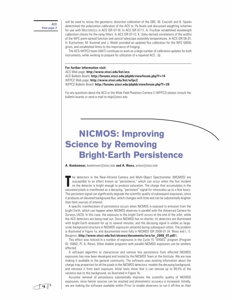
A specific manifestation of persistence occurs when NICMOS is exposed to emission from the bright Earth, which can happen when NICMOS observes in parallel with the Advanced Camera for Surveys (ACS). In this case, the exposure to the bright Earth occurs at the end of the orbit, while the ACS detectors are being read out. Since NICMOS has no shutter, its detectors are illuminated with bright-Earth emission for up to several minutes, and the decaying signal is visible as large-scale background structure in NICMOS exposures obtained during subsequent orbits. The problem is illustrated in Figure 1a, and documented more fully in NICMOS ISR 2008-01 (A. Riess and L. E. Bergeron, http://www.stsci.edu/hst/nicmos/documents/isrs/isr_2008_01.pdf/).

This effect was noticed in a number of exposures in the Cycle 15 “SHOES” program (Program ID: 10802; PI: A. Riess). Other Hubble programs with parallel NICMOS exposures can be similarly affected.

A software algorithm to characterize and remove this persistence from affected NICMOS exposures has now been developed and tested by the NICMOS Team at the Institute. We are now making it available to the general community. The software uses existing information about the charge-trap properties for all the pixels in the NICMOS detectors, models the decaying background, and removes it from each exposure. Initial tests show that it can remove up to 99.5% of the variance due to this background, as illustrated in Figure 1b.

Accurate removal of persistence substantially improves the scientific quality of NICMOS exposures, since fainter sources can be reached and photometric accuracy is increased. Initially, we are making the software available within PYRAF to enable observers to run it off-line on their 4

NICMOS: Improving Science by Removing Bright-Earth PersistenceA. Koekemoer, koekemoer@stsci.edu and A. Riess, ariess@stsci.edu

will be used to revise the geometric distortion calibration of the SBC. M. Cracraft and B. Sparks determined the polarization calibration of the ACS to 1% levels and discussed weighting schemes for use with MULTIDRIZZLE in ACS ISR 07-10. In ACS ISR 07-11, A. Fruchter established wavelength calibration checks for the ramp filters. In ACS ISR 07-12, K. Sahu derived correlations of the widths of the WFC point-spread function and optical telescope assembly temperatures. In ACS ISR 08-01, H. Kuntschner, M. Kummel and J. Walsh provided an updated flux calibration for the WFC G800L grism, and established limits to the importance of fringing.

The ACS-WFPC2 team (AWT) continues to work on a large number of calibration updates for both instruments, while working to prepare for utilization of a repaired ACS. W

For further information visit:ACS Web page: http://www.stsci.edu/hst/acs ACS Bulletin Board: http://forums.stsci.edu/phpbb/viewforum.php?f=14 WFPC2 Web page: http://www.stsci.edu/hst/wfpc2 WFPC2 Bulletin Board: http://forums.stsci.edu/phpbb/viewforum.php?f=20

For any questions about the ACS or the Wide Field Planetary Camera 2 (WFPC2) please consult the bulletin boards or send e-mail to help@stsci.edu.

NICMOS: Improving Science by Removing Bright-Earth Persistence

ACS from page 3

O n August 3, 2004, the Space Telescope Imaging Spectrograph (STIS) was rendered inoperable when a component failed on a circuit board in a low-voltage power supply. This failure made it impossible for STIS to move its mechanisms, and no light could reach the

detectors. At the time, STIS was already operating with the redundant, side-2 electronics because the primary, side-1 electronics had failed previously, in 2001.

Following the 2004 incident, NASA devised a plan to restore STIS to operational status by replacing the failed circuit board during the upcoming Servicing Mission 4 (SM4). The repair will require removing the cover of an electronics box, extracting the failed board, inserting the replacement board, and installing a replacement cover. Initially, plans also included a new radiator to cool the STIS multi-anode multichannel array (MAMA) detectors by several degrees to reduce dark current. NASA dropped this “STIS Cooling System,” however, to devote more time and resources to higher priority activities, including an attempt to restore the charge coupled device (CCD) detectors of the Advanced Camera for Surveys.

The replacement circuit board for STIS—as well as the replacement cover for the electronics box and the tools the astronauts will use to perform the repair—have been manufactured and tested. We currently anticipate that the repair of STIS will occur during the 4th extra-vehicular activity of SM4. After that, brief

STIS Update Charles Proffitt, proffitt@stsci.edu

5

For further information, please visit:NICMOS Web Page: http://www.stsci.edu/hst/nicmos/ NICMOS Bulletin Board: http://forums.stsci.edu/phpbb/viewforum.php?f=13

For any questions about NICMOS please feel free to post a message on the NICMOS Bulletin Board, or send an email message to help@stsci.edu.

own data. We are also investigating whether it may be automatically incorporated into the Hubble NICMOS archival pipeline, which will result in an overall improvement of the long-term scientific legacy value of archival NICMOS data. W

Continuedpage 6

Figure 1. (a) An example of the impact of decaying, persistent bright-Earth emission in a single NICMOS exposure, in this case from Hubble Program 10258, visit 9, obtained using the NIC2 camera. (b) The same exposure after applying the correction software to model and remove the low-level residual emission. It is clear that the quality of the exposure is substantially improved, with the background now being essentially flat.

6

functional and aliveness tests will verify the success of the repair. Testing the actual scientific capabilities of STIS will begin after Hubble is released from the shuttle Discovery.

We expect that the repaired STIS will have capabilities similar to those prior to the failure. Nevertheless, accumulated radiation damage to the detectors and higher temperatures in the aft-shroud of Hubble will probably elevate dark-current levels, as well as increase the number of hot pixels and reduce the charge-transfer efficiency for the STIS CCD detector. Extrapolating the previous trend, we expect the median dark current in the CCD will have increased from a value of 0.0044 e–/s in 2004 to about 0.009 e–/s for Cycle 17, which may significantly affect users observing targets near the faint limit.

For the near-ultraviolet MAMA, the dark current is mostly due to a phosphorescent window glow, and changes to this glow should be modest.

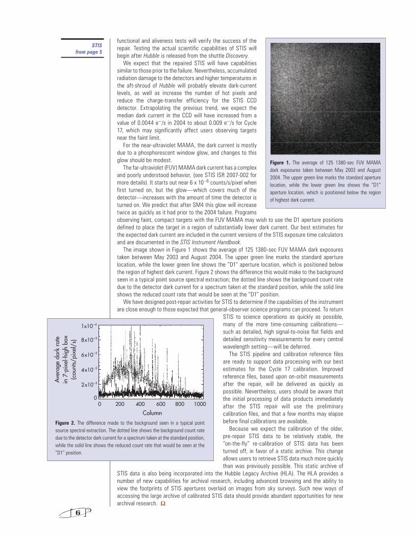
The far-ultraviolet (FUV) MAMA dark current has a complex and poorly understood behavior, (see STIS ISR 2007-002 for more details). It starts out near 6 x 10–6 counts/s/pixel when first turned on, but the glow—which covers much of the detector—increases with the amount of time the detector is turned on. We predict that after SM4 this glow will increase twice as quickly as it had prior to the 2004 failure. Programs observing faint, compact targets with the FUV MAMA may wish to use the D1 aperture positions defined to place the target in a region of substantially lower dark current. Our best estimates for the expected dark current are included in the current versions of the STIS exposure time calculators and are documented in the STIS Instrument Handbook.

The image shown in Figure 1 shows the average of 125 1380-sec FUV MAMA dark exposures taken between May 2003 and August 2004. The upper green line marks the standard aperture location, while the lower green line shows the “D1” aperture location, which is positioned below the region of highest dark current. Figure 2 shows the difference this would make to the background seen in a typical point source spectral extraction; the dotted line shows the background count rate due to the detector dark current for a spectrum taken at the standard position, while the solid line shows the reduced count rate that would be seen at the “D1” position.

We have designed post-repair activities for STIS to determine if the capabilities of the instrument are close enough to those expected that general-observer science programs can proceed. To return

STIS to science operations as quickly as possible, many of the more time-consuming calibrations—such as detailed, high signal-to-noise flat fields and detailed sensitivity measurements for every central wavelength setting—will be deferred.

The STIS pipeline and calibration reference files are ready to support data processing with our best estimates for the Cycle 17 calibration. Improved reference files, based upon on-orbit measurements after the repair, will be delivered as quickly as possible. Nevertheless, users should be aware that the initial processing of data products immediately after the STIS repair will use the preliminary calibration files, and that a few months may elapse before final calibrations are available.

Because we expect the calibration of the older, pre-repair STIS data to be relatively stable, the “on-the-fly” re-calibration of STIS data has been turned off, in favor of a static archive. This change allows users to retrieve STIS data much more quickly than was previously possible. This static archive of

STIS data is also being incorporated into the Hubble Legacy Archive (HLA). The HLA provides a number of new capabilities for archival research, including advanced browsing and the ability to view the footprints of STIS apertures overlaid on images from sky surveys. Such new ways of accessing the large archive of calibrated STIS data should provide abundant opportunities for new archival research. W

STIS from page 5

Figure 1. The average of 125 1380-sec FUV MAMA dark exposures taken between May 2003 and August 2004. The upper green line marks the standard aperture location, while the lower green line shows the “D1” aperture location, which is positioned below the region of highest dark current.

0 200 400 600 800 1000

Ave

rage

dar

k ra

tein

7-p

ixel

-hig

h bo

x(c

ount

s/pi

xel/

s)

Column

0

2x10–5

4x10–5

6x10–5

8x10–5

1x10–4

Figure 2. The difference made to the background seen in a typical point source spectral extraction. The dotted line shows the background count rate due to the detector dark current for a spectrum taken at the standard position, while the solid line shows the reduced count rate that would be seen at the “D1” position.

Improving Hubble’s Pointing and Astrometry M. Lallo, lallo@stsci.edu

A bsolute astrometric accuracy is important in the era of multimission archives and campaigns to cross-match objects observed at different wavelengths by various missions. For example, an astronomer might wish to study Hubble images of the optical counterpart of an X-ray source found by Chandra, or of an infrared source found by Spitzer. Also, the

accuracy of Hubble’s pointing will be operationally crucial after the installation, later this year, of the Cosmic Origins Spectrograph (COS), which has a tiny aperture—1.25 arcseconds in radius.

The accuracy with which a marksman can hit a target depends on the calibration of the gunsight. Likewise, Hubble’s astronomical “sharp shooting” relies on an accurate calibration of its Fine Guidance Sensors (FGSs). To point the telescope, the FGSs lock onto selected guide stars falling into their large, banana-shaped fields of view. The goal of such calibrations is to accurately compute the astrometric position of any point within the field-of-view of a science instrument, given the measured locations of the selected guide stars, whose positions are tabulated in Guide Star Catalog 2 (GSC2).

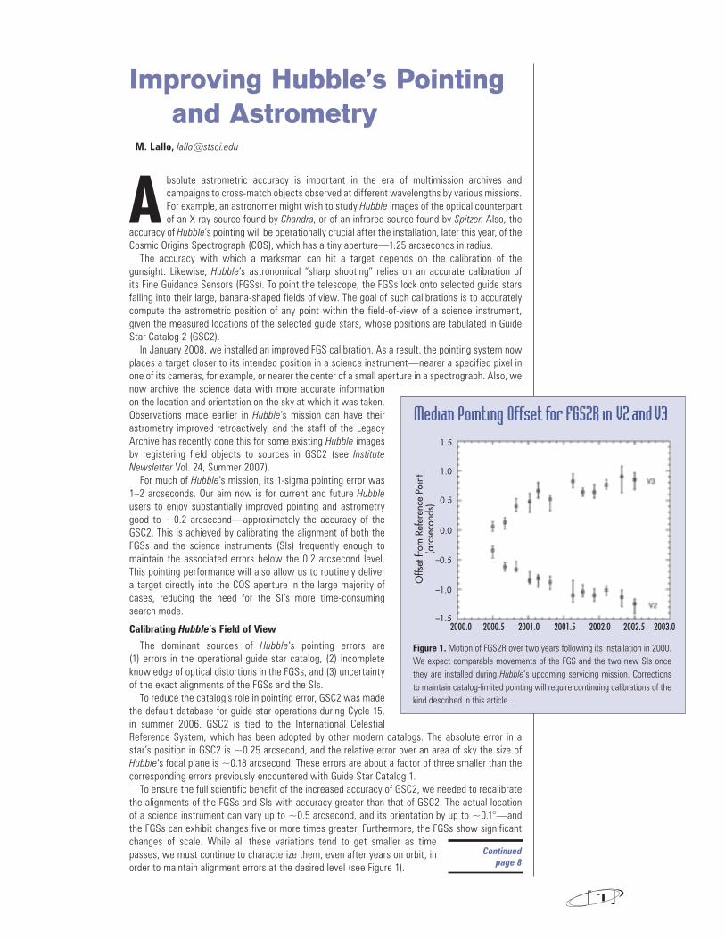
In January 2008, we installed an improved FGS calibration. As a result, the pointing system now places a target closer to its intended position in a science instrument—nearer a specified pixel in one of its cameras, for example, or nearer the center of a small aperture in a spectrograph. Also, we now archive the science data with more accurate information on the location and orientation on the sky at which it was taken. Observations made earlier in Hubble’s mission can have their astrometry improved retroactively, and the staff of the Legacy Archive has recently done this for some existing Hubble images by registering field objects to sources in GSC2 (see Institute Newsletter Vol. 24, Summer 2007).

For much of Hubble’s mission, its 1-sigma pointing error was 1–2 arcseconds. Our aim now is for current and future Hubble users to enjoy substantially improved pointing and astrometry good to ~0.2 arcsecond—approximately the accuracy of the GSC2. This is achieved by calibrating the alignment of both the FGSs and the science instruments (SIs) frequently enough to maintain the associated errors below the 0.2 arcsecond level. This pointing performance will also allow us to routinely deliver a target directly into the COS aperture in the large majority of cases, reducing the need for the SI’s more time-consuming search mode.

Calibrating Hubble’s Field of View

The dominant sources of Hubble’s pointing errors are (1) errors in the operational guide star catalog, (2) incomplete knowledge of optical distortions in the FGSs, and (3) uncertainty of the exact alignments of the FGSs and the SIs.

To reduce the catalog’s role in pointing error, GSC2 was made the default database for guide star operations during Cycle 15, in summer 2006. GSC2 is tied to the International Celestial Reference System, which has been adopted by other modern catalogs. The absolute error in a star’s position in GSC2 is ~0.25 arcsecond, and the relative error over an area of sky the size of Hubble’s focal plane is ~0.18 arcsecond. These errors are about a factor of three smaller than the corresponding errors previously encountered with Guide Star Catalog 1.

To ensure the full scientific benefit of the increased accuracy of GSC2, we needed to recalibrate the alignments of the FGSs and SIs with accuracy greater than that of GSC2. The actual location of a science instrument can vary up to ~0.5 arcsecond, and its orientation by up to ~0.1°—and the FGSs can exhibit changes five or more times greater. Furthermore, the FGSs show significant changes of scale. While all these variations tend to get smaller as time passes, we must continue to characterize them, even after years on orbit, in order to maintain alignment errors at the desired level (see Figure 1).

7

Improving Hubble’s Pointing and Astrometry

Continuedpage 8

2000.0 2000.5 2001.0 2001.5 2002.0 2002.5 2003.0

Median Pointing Offset for FGS2R in V2 & V3

–1.5

–1.0

–0.5

0.0

0.5

1.0

1.5

Offs

et fr

om R

efer

ence

Poi

nt(a

rcse

cond

s)

Figure 1. Motion of FGS2R over two years following its installation in 2000. We expect comparable movements of the FGS and the two new SIs once they are installed during Hubble’s upcoming servicing mission. Corrections to maintain catalog-limited pointing will require continuing calibrations of the kind described in this article.

Median Pointing Offset for FGS2R in V2 and V3

8

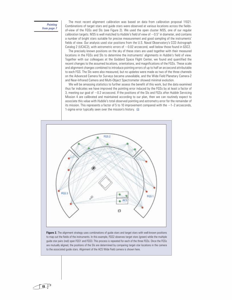
The most recent alignment calibration was based on data from calibration proposal 11021. Combinations of target stars and guide stars were observed at various locations across the fields-of-view of the FGSs and SIs (see Figure 2). We used the open cluster M35, one of our regular calibration targets. M35 is well matched to Hubble’s field of view of ~0.5° in diameter, and contains a number of bright stars suitable for precise measurement and good sampling of the instruments’ fields of view. Our analysis used star positions from the U.S. Naval Observatory’s CCD Astrograph Catalog 2 (UCAC2), with astrometric errors of ~0.02 arcsecond, well below those found in GSC2.

The precisely known positions on the sky of these stars are used together with their measured locations in the FGSs and SIs to determine the instruments’ alignments in Hubble’s field of view. Together with our colleagues at the Goddard Space Flight Center, we found and quantified the recent changes to the assumed locations, orientations, and magnifications of the FGSs. These scale and alignment changes combined to introduce pointing errors of up to half an arcsecond attributable to each FGS. The SIs were also measured, but no updates were made as two of the three channels on the Advanced Camera for Surveys became unavailable, and the Wide Field Planetary Camera-2 and Near-Infrared Camera and Multi-Object Spectrometer showed minimal evolution.

We will be amassing statistics to further assess the benefit of this work, but the data examined thus far indicates we have improved the pointing error induced by the FGSs by at least a factor of 3, meeting our goal of ~0.2 arcsecond. If the positions of the SIs and FGSs after Hubble Servicing Mission 4 are calibrated and maintained according to our plan, then we can routinely expect to associate this value with Hubble’s total observed pointing and astrometry error for the remainder of its mission. This represents a factor of 5 to 10 improvement compared with the ~1–2 arcseconds, 1-sigma error typically seen over the mission’s history. W

Pointing from page 7

Figure 2. The alignment strategy uses combinations of guide stars and target stars with well-known positions to map out the fields of the instruments. In this example, FGS2 observes target stars (green) while the multiple guide star pairs (red) span FGS1 and FGS3. This process is repeated for each of the three FGSs. Once the FGSs are mutually aligned, the positions of the SIs are determined by comparing target-star locations in the camera to the associated guide stars. Alignment of the ACS Wide Field camera is shown here.

WFC3 Status John W. MacKenty, mackenty@stsci.edu

T he Wide Field Camera 3 (WFC3) is fully assembled with its flight detectors and is undergoing final checkouts and calibrations prior to transport to Kennedy Space Center. January 2008 saw the electromagnetic compatibility and interference tests, followed by the Servicing

Mission Ground Test in February. These tests validate WFC3’s compatibility with Hubble, and check our ability to operate it following installation. Also, fit-checks were performed between WFC3 and the High Fidelity Mechanical Simulator and the Wide Field Science Instrument Protective Enclosure (the “box” that protects WFC3 in the shuttle cargo bay). Meanwhile, the Servicing Mission 4 astronauts have been familiarizing themselves with WFC3.

An exhausting, 127-day run of thermal vacuum (TV) testing in summer 2007 tested WFC3 extensively, and validated most subsystems. Issues were discovered with the visible-light calibration lamps, and with the thermal control circuitry for the cooler of the infrared detector. New lamps were procured that corrected a design flaw, and they have completed life testing and are now installed in the instrument. The thermal control circuitry was modified and recent testing has validated its performance.

Both the ultraviolet-visible and infrared detector assemblies have been replaced with much superior flight detectors. The ultraviolet-visible focal plane contains the most sensitive ultraviolet CCD ever manufactured. Further, the packaging of the focal plane has been extensively reworked to mitigate several deficiencies discovered during testing. The infrared detector assembly now contains the finest infrared

Continuedpage 10

9

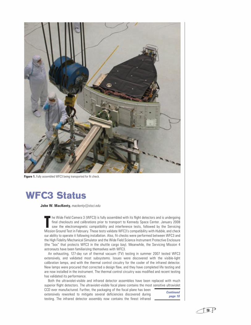
Figure 1. Fully assembled WFC3 being transported for fit check.

detector produced by the Hubble program. It removes susceptibility to proton-induced glow and offers about twice the science performance of the detectors available in 2004. Quantum efficiency at the shorter infrared wavelengths (850–1400 nm) is greatly improved, with essentially flat response over the entire band. Dark current is also well below the Hubble and zodiacal light background in the broad band filters.

A final TV test in February–April 2008 has obtained the flight science calibrations and completed the optical, thermal, and operations validation of WFC3 for flight.

Observer support activities for WFC3 are ramping up. The Instrument Handbook was released as part of the Cycle 17 Call for Proposals. WFC3 now has APT support, an exposure time calculator, and, thanks to our colleagues at the ST-ECF, a grism simulator for spectroscopic observations. The WFC3 data pipeline is included in the upcoming STSDAS release. W

10

WFC3 from page 9

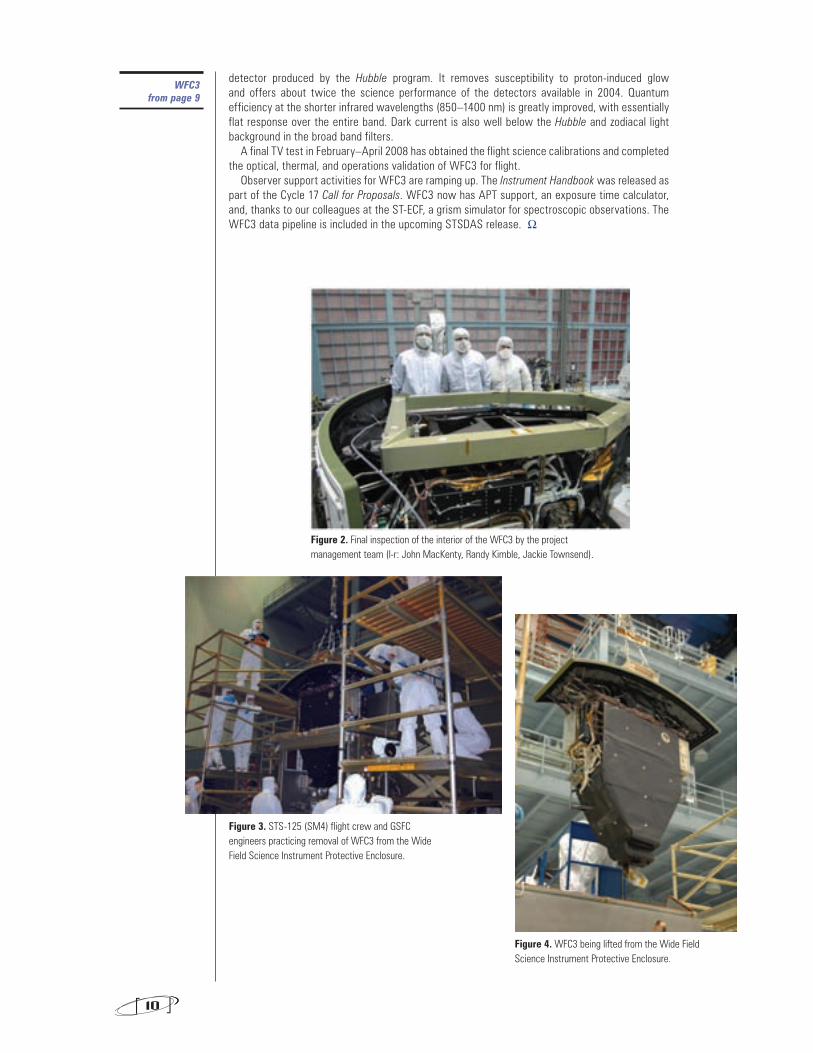
Figure 3. STS-125 (SM4) flight crew and GSFC engineers practicing removal of WFC3 from the Wide Field Science Instrument Protective Enclosure.

Figure 2. Final inspection of the interior of the WFC3 by the project management team (l-r: John MacKenty, Randy Kimble, Jackie Townsend).

Figure 4. WFC3 being lifted from the Wide Field Science Instrument Protective Enclosure.

COS Status Tony Keyes, keyes@stsci.edu

P reparations are proceeding rapidly to install the Cosmic Origins Spectrograph (COS) on Hubble during Servicing Mission 4 (SM4), and to conduct science observations with COS during Cycle 17. To support the Cycle 17 Call for Proposals (CP) in December 2007, the Institute issued

the first COS Instrument Handbook (IHB) and released the COS Exposure Time Calculator (ETC) for spectroscopy, imaging, and all types of target acquisition.

The Institute is ramping up support for COS users on several fronts. Following the distribution of the CP, the Institute helpdesk fielded many COS questions. At the January AAS meeting in Austin, the Institute’s COS instrument scientists presented posters about optimizing TIME-TAG observations, bright-object protection, target acquisition, pipeline calibration, and output data formats. COS team members helped distribute the latest version of the instrument information brochure, and they were available continuously at the Institute booth to answer questions from potential COS observers.

Regarding COS hardware and operations, the Institute developed a suite of programs to test the end-to-end performance of the ground systems. These tests were run on the instrument at Goddard Space Flight Center (GSFC). Engineers at Ball Aerospace and GSFC have now completed hardware testing and made changes to the flight software to make instrument turn-on more robust.

The COS principal investigator, Dr. James Green of the University of Colorado, leads the Instrument Development Team (IDT). The Institute collaborates with the IDT to craft early programs for instrument startup, checkout, and optical alignment, followed by calibration and characterization programs to verify the scientific performance of COS. The IDT has delivered the first suite of calibration reference files, which will be used in the calibration pipeline to process data from early observations. Updated reference files, based upon on-orbit performance, will be delivered as COS is better characterized in the servicing mission observatory verification period immediately after SM4 and in the early stages of the Cycle 17 calibration program. Users should be aware that early COS science observations will be processed initially using the best-available—but preliminary—calibration information, and that it will take a few months before all on-orbit calibrations are available through the “on-the-fly” recalibration of the Hubble archive.

Also in collaboration with the IDT, the Institute has developed a comprehensive plan for pipeline verification. We are developing the COS Data Handbook, which we plan to publish in December 2008, to support the beginning of COS science operations.

The COS IHB, ETC, instrument brochure, and a variety of additional user-support information are available via the Institute COS instrument website (http://www.stsci.edu/hst/cos) W

Continuedpage 12

11

COS Optical Design

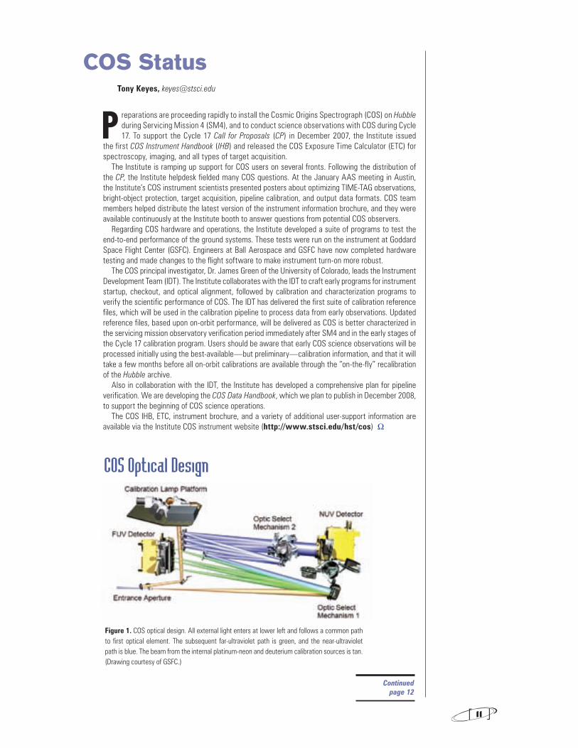
Figure 1. COS optical design. All external light enters at lower left and follows a common path to first optical element. The subsequent far-ultraviolet path is green, and the near-ultraviolet path is blue. The beam from the internal platinum-neon and deuterium calibration sources is tan. (Drawing courtesy of GSFC.)

12

COSfrom page 11

Just before Christmas 2007, the verification model (VM) of the Webb Mid Infrared Instrument (MIRI) started thermal-vacuum testing at the Rutherford Appleton Laboratory (RAL) in the United Kingdom. The VM is a

functioning, flight-like version of the instrument, built for a variety of purposes, including: (1) demonstrating processes and procedures for manufacturing, assembly, and alignment; (2) developing methods for testing and calibrating the flight model; and (3) testing end-to-end functionality, from commanding the flight software through the receipt of data. We are testing the MIRI VM to build confidence in the design—both in terms of science and of operations. Within the limitations of the fidelity standards for the VM, we want confidence that the flight model (FM) of MIRI will meet its functional, performance, and interface requirements.

Although the VM is a fully functioning instrument, it differs from the FM in a number of areas. For instance, the mechanisms and focal planes are not designed to withstand launch vibrations. Also, only the short-wavelength channel of the spectrometer (the most difficult one) is populated with optics, and not all of the filters in the imager are installed.

1100 1200 1300 1400 1500 1600 1700 1800 1900–15.5

–15.0

–14.5

–14.0

–13.5

–13.0

–12.5

log

Flux

(erg

cm

–2 s

ec–1

Å–1

)

Wavelength (Å)

STIS E140M +0.2x0.2 apertureR=45,000

COS G130MR~20,000–24,000

COS G160MR~20,000–24,000

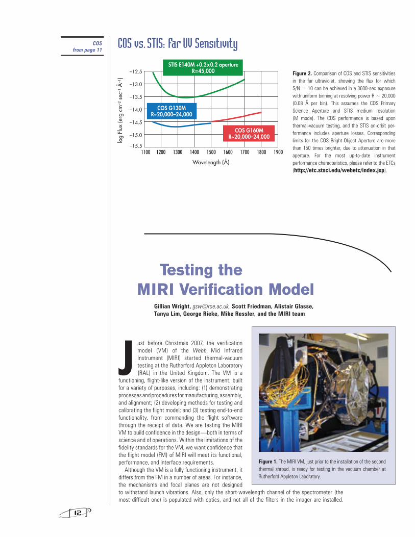
COS vs. STIS: Far UV Sensitivity

Figure 2. Comparison of COS and STIS sensitivities in the far ultraviolet, showing the flux for which S/N = 10 can be achieved in a 3600-sec exposure with uniform binning at resolving power R ~ 20,000 (0.08 Å per bin). This assumes the COS Primary Science Aperture and STIS medium resolution (M mode). The COS performance is based upon thermal-vacuum testing, and the STIS on-orbit per-formance includes aperture losses. Corresponding limits for the COS Bright-Object Aperture are more than 150 times brighter, due to attenuation in that aperture. For the most up-to-date instrument performance characteristics, please refer to the ETCs (http://etc.stsci.edu/webetc/index.jsp).

Testing the MIRI Verification Model

Testing the MIRI Verification Model Gillian Wright, gsw@roe.ac.uk, Scott Friedman, Alistair Glasse, Tanya Lim, George Rieke, Mike Ressler, and the MIRI team

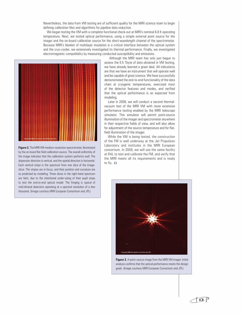
Figure 1. The MIRI VM, just prior to the installation of the second thermal shroud, is ready for testing in the vacuum chamber at Rutherford Appleton Laboratory.

Nevertheless, the data from VM testing are of sufficient quality for the MIRI science team to begin defining calibration files and algorithms for pipeline data reduction.

We began testing the VM with a complete functional check-out at MIRI’s nominal 6.8 K operating temperature. Next, we tested optical performance, using a simple external point source for the imager and the on-board calibration source for the short-wavelength channel of the spectrometer. Because MIRI’s blanket of multilayer insulation is a critical interface between the optical system and the cryo-cooler, we extensively investigated its thermal performance. Finally, we investigated electromagnetic compatibility by measuring conducted susceptibility and emissions.

Although the MIRI team has only just begun to assess the 0.5 Tbyte of data obtained in VM testing, we have already learned a great deal. All indications are that we have an instrument that will operate well and be capable of great science. We have successfully demonstrated the end-to-end functionality of the data chain at cryogenic temperatures, exercised most of the detector features and modes, and verified that the optical performance is as expected from modeling.

Later in 2008, we will conduct a second thermal-vacuum test of the MIRI VM with more extensive performance testing enabled by the MIRI telescope simulator. This simulator will permit point-source illumination of the imager and spectrometer anywhere in their respective fields of view, and will also allow for adjustment of the source temperature and for flat-field illumination of the imager.

While the VM is being tested, the construction of the FM is well underway at the Jet Propulsion Laboratory and institutes in the MIRI European consortium. In 2009, we will use the same facility at RAL to test and calibrate the FM, and verify that the MIRI meets all its requirements and is ready to fly. W

13

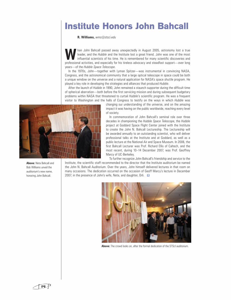
Figure 2. The MIRI VM medium-resolution spectrometer, illuminated by the on-board flat-field calibration source. The overall uniformity of the image indicates that the calibration system performs well. The dispersion direction is vertical, and the spatial direction is horizontal. Each vertical stripe is the spectrum from one slice of the image-slicer. The stripes are in focus, and their position and curvature are as predicted by modeling. Three slices in the right-hand spectrum are faint, due to the intentional under-sizing of their pupil stops to test the end-to-end optical model. The fringing is typical of mid-infrared detectors operating at a spectral resolution of a few thousand. (Image courtesy MIRI European Consortium and JPL)

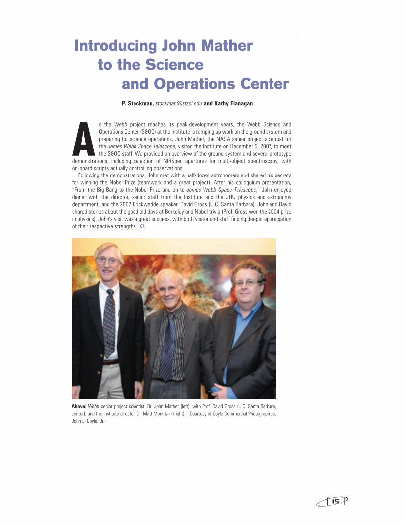
Figure 3. A point-source image from the MIRI VM imager. Initial analysis confirms that the optical performance meets the design goals. (Image courtesy MIRI European Consortium and JPL)

14

W hen John Bahcall passed away unexpectedly in August 2005, astronomy lost a true leader, and the Hubble and the Institute lost a great friend. John was one of the most influential scientists of his time. He is remembered for many scientific discoveries and

professional activities, and especially for his tireless advocacy and steadfast support—over long years—of the Hubble Space Telescope.

In the 1970s, John—together with Lyman Spitzer—was instrumental in convincing NASA, Congress, and the astronomical community that a large optical telescope in space could be both a unique window on the universe and a natural application for NASA’s space shuttle program. He played a key role in developing the strategies and alliances that produced Hubble.

After the launch of Hubble in 1990, John remained a staunch supporter during the difficult time of spherical aberration—both before the first servicing mission and during subsequent budgetary problems within NASA that threatened to curtail Hubble’s scientific program. He was a frequent visitor to Washington and the halls of Congress to testify on the ways in which Hubble was

changing our understanding of the universe, and on the amazing impact it was having on the public worldwide, reaching every level of society.

In commemoration of John Bahcall’s seminal role over three decades in championing the Hubble Space Telescope, the Hubble project at Goddard Space Flight Center joined with the Institute to create the John N. Bahcall Lectureship. The Lectureship will be awarded annually to an outstanding scientist, who will deliver professional talks at the Institute and at Goddard, as well as a public lecture at the National Air and Space Museum. In 2006, the first Bahcall Lecturer was Prof. Richard Ellis of Caltech, and the most recent, during 10–14 December 2007, was Prof. Geoffrey Marcy of UC-Berkeley.

To further recognize John Bahcall’s friendship and service to the Institute, the scientific staff recommended to the director that the Institute auditorium be named the John N. Bahcall Auditorium. Over the years, John himself delivered lectures in that room on many occasions. The dedication occurred on the occasion of Geoff Marcy’s lecture in December 2007, in the presence of John’s wife, Neta, and daughter, Orli. W

Institute Honors John Bahcall R. Williams, wms@stsci.edu

Above: Neta Bahcall and Bob Williams unveil the auditorium’s new name, honoring John Bahcall.

Above: The crowd looks on, after the formal dedication of the STScI auditorium.

As the Webb project reaches its peak-development years, the Webb Science and Operations Center (S&OC) at the Institute is ramping up work on the ground system and preparing for science operations. John Mather, the NASA senior project scientist for the James Webb Space Telescope, visited the Institute on December 5, 2007, to meet the S&OC staff. We provided an overview of the ground system and several prototype

demonstrations, including selection of NIRSpec apertures for multi-object spectroscopy, with on-board scripts actually controlling observations.

Following the demonstrations, John met with a half-dozen astronomers and shared his secrets for winning the Nobel Prize (teamwork and a great project). After his colloquium presentation, “From the Big Bang to the Nobel Prize and on to James Webb Space Telescope,” John enjoyed dinner with the director, senior staff from the Institute and the JHU physics and astronomy department, and the 2007 Brickwedde speaker, David Gross (U.C. Santa Barbara). John and David shared stories about the good old days at Berkeley and Nobel trivia (Prof. Gross won the 2004 prize in physics). John’s visit was a great success, with both visitor and staff finding deeper appreciation of their respective strengths. W

15

Introducing John Mather to the Science and Operations Center P. Stockman, stockman@stsci.edu and Kathy Flanagan

Introducing John Mather to the Science Operations Center

Above: Webb senior project scientist, Dr. John Mather (left), with Prof. David Gross (U.C. Santa Barbara, center), and the Institute director, Dr. Matt Mountain (right). (Courtesy of Coyle Commercial Photographics, John J. Coyle, Jr.)

16

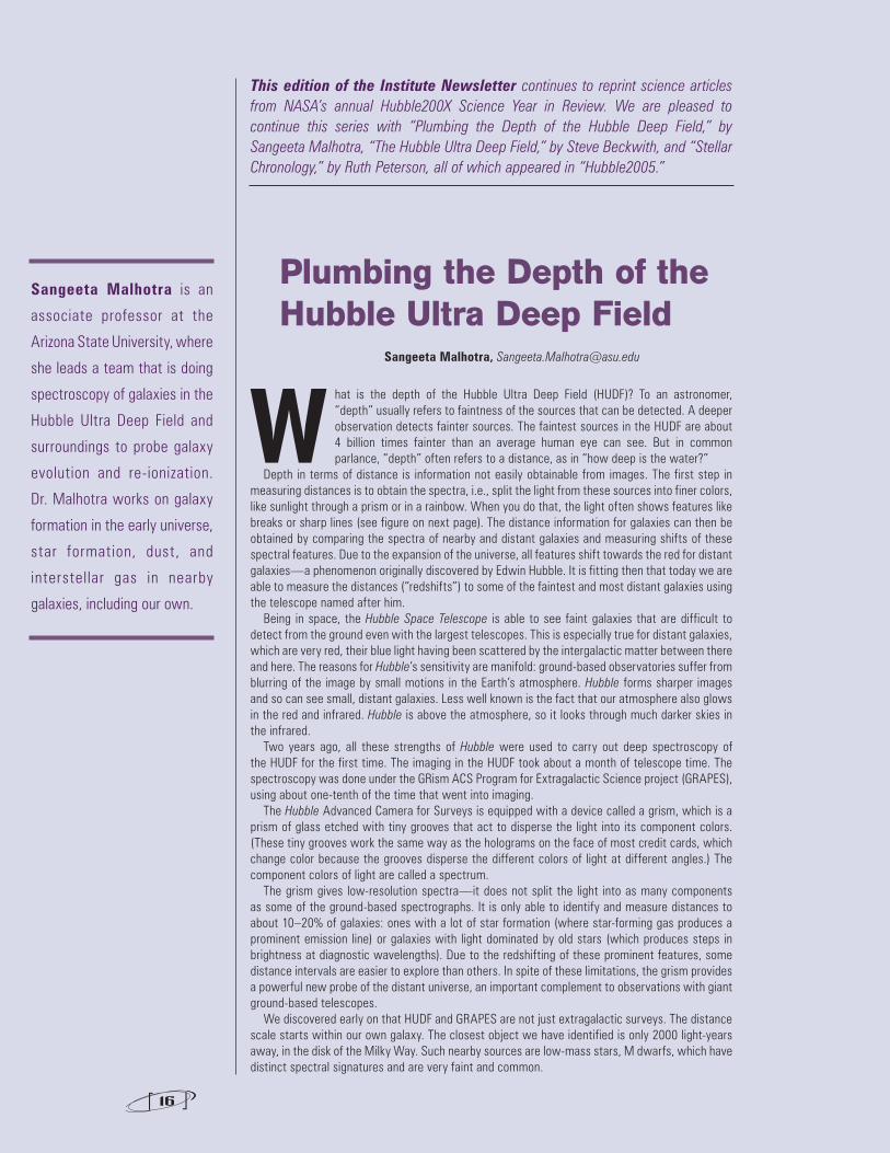
Plumbing the Depth of the Hubble Ultra Deep Field Sangeeta Malhotra, Sangeeta.Malhotra@asu.edu

What is the depth of the Hubble Ultra Deep Field (HUDF)? To an astronomer, “depth” usually refers to faintness of the sources that can be detected. A deeper observation detects fainter sources. The faintest sources in the HUDF are about 4 billion times fainter than an average human eye can see. But in common parlance, “depth” often refers to a distance, as in “how deep is the water?”

Depth in terms of distance is information not easily obtainable from images. The first step in measuring distances is to obtain the spectra, i.e., split the light from these sources into finer colors, like sunlight through a prism or in a rainbow. When you do that, the light often shows features like breaks or sharp lines (see figure on next page). The distance information for galaxies can then be obtained by comparing the spectra of nearby and distant galaxies and measuring shifts of these spectral features. Due to the expansion of the universe, all features shift towards the red for distant galaxies—a phenomenon originally discovered by Edwin Hubble. It is fitting then that today we are able to measure the distances (“redshifts”) to some of the faintest and most distant galaxies using the telescope named after him.

Being in space, the Hubble Space Telescope is able to see faint galaxies that are difficult to detect from the ground even with the largest telescopes. This is especially true for distant galaxies, which are very red, their blue light having been scattered by the intergalactic matter between there and here. The reasons for Hubble’s sensitivity are manifold: ground-based observatories suffer from blurring of the image by small motions in the Earth’s atmosphere. Hubble forms sharper images and so can see small, distant galaxies. Less well known is the fact that our atmosphere also glows in the red and infrared. Hubble is above the atmosphere, so it looks through much darker skies in the infrared.

Two years ago, all these strengths of Hubble were used to carry out deep spectroscopy of the HUDF for the first time. The imaging in the HUDF took about a month of telescope time. The spectroscopy was done under the GRism ACS Program for Extragalactic Science project (GRAPES), using about one-tenth of the time that went into imaging.

The Hubble Advanced Camera for Surveys is equipped with a device called a grism, which is a prism of glass etched with tiny grooves that act to disperse the light into its component colors. (These tiny grooves work the same way as the holograms on the face of most credit cards, which change color because the grooves disperse the different colors of light at different angles.) The component colors of light are called a spectrum.

The grism gives low-resolution spectra—it does not split the light into as many components as some of the ground-based spectrographs. It is only able to identify and measure distances to about 10–20% of galaxies: ones with a lot of star formation (where star-forming gas produces a prominent emission line) or galaxies with light dominated by old stars (which produces steps in brightness at diagnostic wavelengths). Due to the redshifting of these prominent features, some distance intervals are easier to explore than others. In spite of these limitations, the grism provides a powerful new probe of the distant universe, an important complement to observations with giant ground-based telescopes.

We discovered early on that HUDF and GRAPES are not just extragalactic surveys. The distance scale starts within our own galaxy. The closest object we have identified is only 2000 light-years away, in the disk of the Milky Way. Such nearby sources are low-mass stars, M dwarfs, which have distinct spectral signatures and are very faint and common.

This edition of the Institute Newsletter continues to reprint science articles from NASA’s annual Hubble200X Science Year in Review. We are pleased to continue this series with “Plumbing the Depth of the Hubble Deep Field,” by Sangeeta Malhotra, “The Hubble Ultra Deep Field,” by Steve Beckwith, and “Stellar Chronology,” by Ruth Peterson, all of which appeared in “Hubble2005.”

Sangeeta Malhotra is an

associate professor at the

Arizona State University, where

she leads a team that is doing

spectroscopy of galaxies in the

Hubble Ultra Deep Field and

surroundings to probe galaxy

evolution and re-ionization.

Dr. Malhotra works on galaxy

formation in the early universe,

star formation, dust, and

interstellar gas in nearby

galaxies, including our own.

Plumbing the Depth of the Hubble Ultra Deep Field

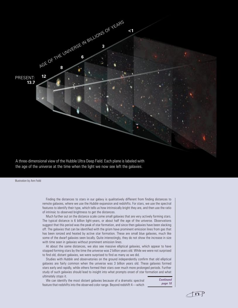
Illustration by Ann Feild

Finding the distances to stars in our galaxy is qualitatively different from finding distances to remote galaxies, where we use the Hubble expansion and redshifts. For stars, we use the spectral features to identify their type, which tells us how intrinsically bright they are, and then use the ratio of intrinsic to observed brightness to get the distances.

Much further out on the distance scale come small galaxies that are very actively forming stars. The typical distance is 6 billion light-years, or about half the age of the universe. Observations suggest that this period was the peak of star formation, and since then galaxies have been slacking off. The galaxies that can be identified with the grism have prominent emission lines from gas that has been ionized and heated by active star formation. These are small blue galaxies, much like some of the dwarf galaxies seen locally. Quite interestingly, they do not show the increase in size with time seen in galaxies without prominent emission lines.

At about the same distances, we also see massive elliptical galaxies, which appear to have stopped forming stars by the time the universe was 2 billion years old. While we were not surprised to find old, distant galaxies, we were surprised to find as many as we did.

Studies with Hubble and observatories on the ground independently confirm that old elliptical galaxies are fairly common when the universe was 3 billion years old. These galaxies formed stars early and rapidly, while others formed their stars over much more prolonged periods. Further study of such galaxies should lead to insight into what prompts onset of star formation and what ultimately stops it.

We can identify the most distant galaxies because of a dramatic spectral feature that redshifts into the observed color range. Beyond redshift 4—which

17

A three-dimensional view of the Hubble Ultra Deep Field. Each plane is labeled with the age of the universe at the time when the light we now see left the galaxies.

AGE OF THE UNIVERSE IN BILLIONS OF YEARS

PRESENT: 13.7

12

8

6

3

<1

Continuedpage 18

corresponds to about 1.5 billion years after the Big Bang—we can measure the distances of all star-forming galaxies. In the HUDF, we see about 50 galaxies at these great distances—seeing them as they were 12 to 12.8 billion years in the past, when the light reaching us today began its journey. These are some of the most distant galaxies ever seen. Because the HUDF goes very faint, we are able to study the typical galaxies at those distances.

Looking at the colors of these remote galaxies reveals their youth; they have younger stars than the galaxies that we see in the nearby, older universe. The appearance of these young galaxies is ragged and irregular, partly because we are originally seeing them in ultraviolet light, and partly because they are still in the process of formation. Untangling the two effects will be valuable.

Because spectra give accurate distances to galaxies, we can discern how they are distributed in three dimensions. We find that galaxies are clustered wherever we have been able to look. In the HUDF, we see a cluster or “wall” of galaxies at a distance of 8 billion light-years (redshift 0.67). Massive, old, elliptical galaxies dominate dense regions at this distance, just as in the local universe. We also see the primitive form of such a cluster at a lookback time of 12.6 billion years away (at redshift ~6), where we find four times as many galaxies as expected. If we looked at some other part of the sky we likely would not see such an aggregation. In fact, this clump covers only half of the HUDF. To see how far this over-density extends, we obtained wide-field imaging at the ground-based telescopes of the National Optical Astronomy Observatory in Chile. At redshift 5.8, which is accessible from the ground, we see a wall of galaxies with a transverse size of at least 20 million light-years. The HUDF is situated at the edge of this distribution.

One of the main motives for the deep imaging of the HUDF was to take a census of galaxies at redshift 6 (a lookback time of 12.6 billion years). A massive ionization of the diffuse intergalactic gas may have occurred at this epoch (as discussed in the article by Steven Beckwith). A census would determine whether the galaxies could provide enough ultraviolet light to ionize the gas. There is some controversy over the counting of redshift-6 galaxies based on the images alone. One set of published estimates says that there are not enough galaxies to ionize the gas. A second group

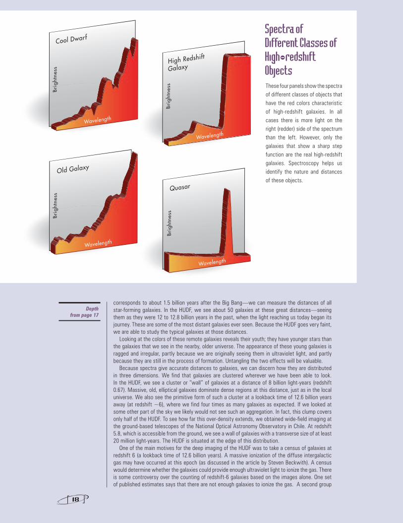
These four panels show the spectra of different classes of objects that have the red colors characteristic of high-redshift galaxies. In all cases there is more light on the right (redder) side of the spectrum than the left. However, only the galaxies that show a sharp step function are the real high-redshift galaxies. Spectroscopy helps us identify the nature and distances of these objects.

Depth from page 17

18

Spectra of Different Classes of High-redshift Objects

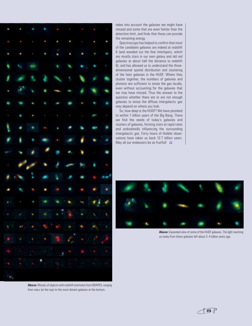
Above: Mosaic of objects with redshift estimates from GRAPES, ranging from stars (at the top) to the most distant galaxies at the bottom.

Above: Expanded view of some of the HUDF galaxies. The light reaching us today from these galaxies left about 3–4 billion years ago.

takes into account the galaxies we might have missed and some that are even fainter than the detection limit, and finds that these can provide the remaining energy.

Spectroscopy has helped to confirm that most of the candidate galaxies are indeed at redshift 6 (and weeded out the few interlopers, which are mostly stars in our own galaxy and old red galaxies at about half the distance to redshift 6), and has allowed us to understand the three-dimensional spatial distribution and clustering of the faint galaxies in the HUDF. Where they cluster together, the numbers of galaxies and photons are sufficient to ionize the gas locally, even without accounting for the galaxies that we may have missed. Thus the answer to the question whether there are or are not enough galaxies to ionize the diffuse intergalactic gas may depend on where you look.

So, how deep is the HUDF? We have plumbed to within 1 billion years of the Big Bang. There we find the seeds of today’s galaxies and clusters of galaxies, forming stars at rapid rates and undoubtedly influencing the surrounding intergalactic gas. Forty hours of Hubble obser-vations have taken us back 12.7 billion years. May all our endeavors be as fruitful! W

19

20

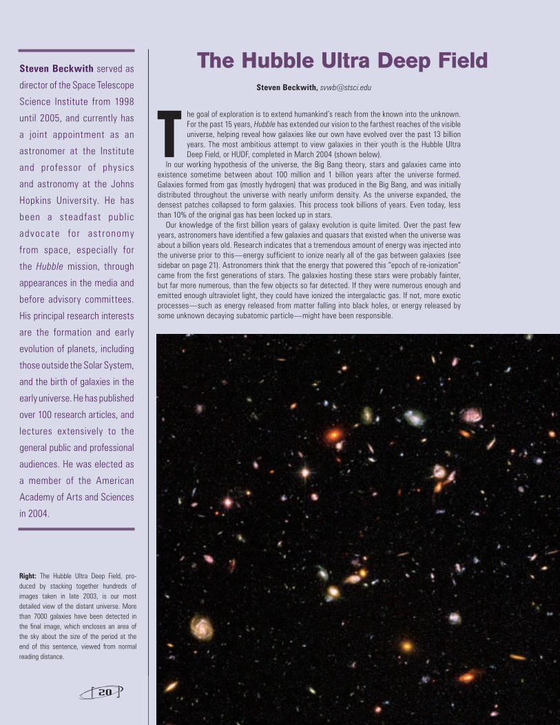
The goal of exploration is to extend humankind’s reach from the known into the unknown. For the past 15 years, Hubble has extended our vision to the farthest reaches of the visible universe, helping reveal how galaxies like our own have evolved over the past 13 billion years. The most ambitious attempt to view galaxies in their youth is the Hubble Ultra Deep Field, or HUDF, completed in March 2004 (shown below).

In our working hypothesis of the universe, the Big Bang theory, stars and galaxies came into existence sometime between about 100 million and 1 billion years after the universe formed. Galaxies formed from gas (mostly hydrogen) that was produced in the Big Bang, and was initially distributed throughout the universe with nearly uniform density. As the universe expanded, the densest patches collapsed to form galaxies. This process took billions of years. Even today, less than 10% of the original gas has been locked up in stars.

Our knowledge of the first billion years of galaxy evolution is quite limited. Over the past few years, astronomers have identified a few galaxies and quasars that existed when the universe was about a billion years old. Research indicates that a tremendous amount of energy was injected into the universe prior to this—energy sufficient to ionize nearly all of the gas between galaxies (see sidebar on page 21). Astronomers think that the energy that powered this “epoch of re-ionization” came from the first generations of stars. The galaxies hosting these stars were probably fainter, but far more numerous, than the few objects so far detected. If they were numerous enough and emitted enough ultraviolet light, they could have ionized the intergalactic gas. If not, more exotic processes—such as energy released from matter falling into black holes, or energy released by some unknown decaying subatomic particle—might have been responsible.

The Hubble Ultra Deep Field Steven Beckwith, svwb@stsci.edu

Steven Beckwith served as

director of the Space Telescope

Science Institute from 1998

until 2005, and currently has

a joint appointment as an

astronomer at the Institute

and professor of physics

and astronomy at the Johns

Hopkins University. He has

been a stead fast publ ic

advocate for as t ronomy

from space, especially for

the Hubble mission, through

appearances in the media and

before advisory committees.

His principal research interests

are the formation and early

evolution of planets, including

those outside the Solar System,

and the birth of galaxies in the

early universe. He has published

over 100 research articles, and

lectures extensively to the

general public and professional

audiences. He was elected as

a member of the American

Academy of Arts and Sciences

in 2004.

Right: The Hubble Ultra Deep Field, pro-duced by stacking together hundreds of images taken in late 2003, is our most detailed view of the distant universe. More than 7000 galaxies have been detected in the final image, which encloses an area of the sky about the size of the period at the end of this sentence, viewed from normal reading distance.

With Hubble, we can, in principle, detect galaxies that are so distant that the light reaching us today began its journey during the epoch of re-ionization. A census of these objects could help determine whether the energy emitted by young galaxies was sufficient to ionize the intergalactic gas. But finding them is a challenge even for Hubble.

Prior to the HUDF, our most sensitive observations were the Deep Fields, taken in 1995 and 1998. These observations provided a wealth of information on distant galaxies, but could detect very few galaxies at look-back times (the time from then until the present) greater than 12 billion years. Such galaxies were generally too faint to detect, and most of the light reaching us from these galaxies was at wavelengths redder than Hubble’s camera could detect. The Advanced Camera for Surveys (ACS), installed in 2002, provided the opportunity for Hubble to detect galaxies at least six times fainter. It is especially sensitive to faint red galaxies.

Creating the next-generation deep field, the HUDF, was a great adventure drawing on the expertise of astronomers from around the world. Hubble pointed at a spot in the constellation of Fornax and took observations over a span of 40 days starting in September 2003, paused for a month, and observed for another span of 40 days until January 16, 2004. The final exposure lasted one million seconds, the longest exposure ever taken with an optical telescope, and using all of the Institute Director’s discretionary time for one year. The release of the images on March 9, 2004, generated tremendous interest among both astronomers and the general public (nearly saturating the Space Telescope Science Institute’s internet connection for a few days). A group led by Rodger Thompson of the University 21

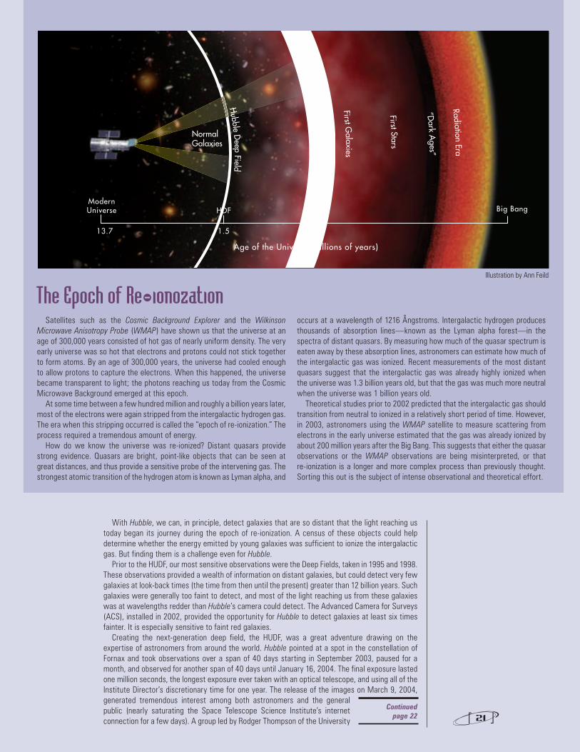
The Epoch of Re-ionozation

Continuedpage 22

Satellites such as the Cosmic Background Explorer and the Wilkinson Microwave Anisotropy Probe (WMAP) have shown us that the universe at an age of 300,000 years consisted of hot gas of nearly uniform density. The very early universe was so hot that electrons and protons could not stick together to form atoms. By an age of 300,000 years, the universe had cooled enough to allow protons to capture the electrons. When this happened, the universe became transparent to light; the photons reaching us today from the Cosmic Microwave Background emerged at this epoch.

At some time between a few hundred million and roughly a billion years later, most of the electrons were again stripped from the intergalactic hydrogen gas. The era when this stripping occurred is called the “epoch of re-ionization.” The process required a tremendous amount of energy.

How do we know the universe was re-ionized? Distant quasars provide strong evidence. Quasars are bright, point-like objects that can be seen at great distances, and thus provide a sensitive probe of the intervening gas. The strongest atomic transition of the hydrogen atom is known as Lyman alpha, and

occurs at a wavelength of 1216 Ångstroms. Intergalactic hydrogen produces thousands of absorption lines—known as the Lyman alpha forest—in the spectra of distant quasars. By measuring how much of the quasar spectrum is eaten away by these absorption lines, astronomers can estimate how much of the intergalactic gas was ionized. Recent measurements of the most distant quasars suggest that the intergalactic gas was already highly ionized when the universe was 1.3 billion years old, but that the gas was much more neutral when the universe was 1 billion years old.

Theoretical studies prior to 2002 predicted that the intergalactic gas should transition from neutral to ionized in a relatively short period of time. However, in 2003, astronomers using the WMAP satellite to measure scattering from electrons in the early universe estimated that the gas was already ionized by about 200 million years after the Big Bang. This suggests that either the quasar observations or the WMAP observations are being misinterpreted, or that re-ionization is a longer and more complex process than previously thought. Sorting this out is the subject of intense observational and theoretical effort.

Illustration by Ann Feild

RadiationEr a

“Dark A

ges ”

F irs t Stars

First Gal ax ies

bble Deep Field

Normal Galaxies

9.0 5.1 7.31

Modern Universe HDF HUDF Big Bang

Age of the Universe (billions of years)

Epoch of Re- ioni zation

22

of Arizona carried out an additional set of observations with Hubble’s Near Infrared Camera and Multi-Object Spectrometer (NICMOS), providing the opportunity to search for even redder galaxies. Another group, led by Sangeeta Malhotra of the Space Telescope Science Institute, used ACS to measure galaxy spectra.

In the HUDF, we can see the entire span of the universe’s history, from less than a billion years after the Big Bang until the present day. The faintest objects are roughly 4 billion times fainter than those we can see with the unaided eye. The smallest are only 50 milliseconds of arc across, equivalent to the size of a dime seen from a distance of 50 miles. The HUDF is an image of superlatives: the deepest, farthest, and earliest look into the history of stars and galaxies.

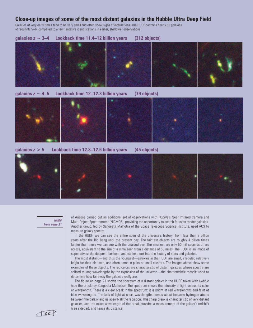
The most distant—and thus the youngest—galaxies in the HUDF are small, irregular, relatively bright for their distance, and often come in pairs or small clusters. The images above show some examples of these objects. The red colors are characteristic of distant galaxies whose spectra are shifted to long wavelengths by the expansion of the universe—the characteristic redshift used to determine how far away the galaxies really are.

The figure on page 23 shows the spectrum of a distant galaxy in the HUDF taken with Hubble (see the article by Sangeeta Malhotra). The spectrum shows the intensity of light versus its color or wavelength. There is a clear break in the spectrum: it is bright at red wavelengths and faint at blue wavelengths. The lack of light at short wavelengths comes about because hydrogen atoms between the galaxy and us absorb all the radiation. This sharp break is characteristic of very distant galaxies, and the exact wavelength of the break provides a measurement of the galaxy’s redshift (see sidebar), and hence its distance.

Close-up images of some of the most distant galaxies in the Hubble Ultra Deep Field

galaxies z ~ 3–4 Lookback time 11.4–12 billion years (312 objects)

galaxies z ~ 4–5 Lookback time 12–12.3 billion years (79 objects)

galaxies z > 5 Lookback time 12.3–12.6 billion years (45 objects)

Galaxies at very early times tend to be very small and often show signs of interactions. The HUDF contains nearly 50 galaxies at redshifts 5–6, compared to a few tentative identifications in earlier, shallower observations.

HUDF from page 21

23

Most of the galaxies in the HUDF are so faint that we cannot measure their spectra. Nevertheless, we do have good measurements of their colors from the four filters used to take the image. Those colors provide rough estimates of galaxy redshifts, and thus, distances. They allow us to count the number of galaxies as a function of lookback time. Moreover, we can use the observed brightness of the galaxies to estimate how much radiation they emitted at different times to compare with the amount needed to re-ionize the universe.

The census of distant galaxies in the HUDF indicates that young galaxies may provide almost enough energy to account for the ionization of the universe. But different groups of astronomers analyzing both the ACS and the NICMOS HUDF observations have come to different conclusions about whether the energy is actually sufficient.

Three complications have led to controversy when analyzing the images. The first is that we cannot actually measure the amount of radiation that provides the ionization, because it is all at wavelengths much shorter than we can observe. To ionize hydrogen, light must be at a wavelength shorter than 912 Å. We must extrapolate from the light we receive at longer wavelengths to estimate the amount emitted at shorter wavelengths. The assumptions used to extrapolate the galaxy spectra depend on the ages and chemical abundances assumed for the stars in these galaxies, and are a matter of debate.

The second complication is that the light from many faint galaxies—that we cannot see—might be the most important source of ionizing radiation. In the nearby universe, we know that small (dwarf) galaxies outnumber large ones. There are hints in the HUDF that small galaxies might have outnumbered large ones by an even larger factor in the past.

The galaxies that we see may just be the tip of the iceberg, so to speak, an indication of many more unseen galaxies that are, nevertheless, important to the ionization of the universe. Estimating the number of these faint galaxies also requires an extrapolation from what we see, and the assumptions used here are uncertain and controversial.

RedshiftsThe expansion of the universe stretches the light waves emitted from

distant galaxies during their passage to Earth. The light “redshifts”—changes to longer wavelengths—because the light waves are stretched by the expansion of universe. For very distant galaxies, blue light becomes red, and red light becomes infrared.

Astronomers can use this “cosmological” redshift to estimate the distances to galaxies: the larger the shift, the greater the distance. To do this precisely, astronomers disperse the light of a distant galaxy into a spectrum and look for the telltale signatures of atoms, such as hydrogen and oxygen.

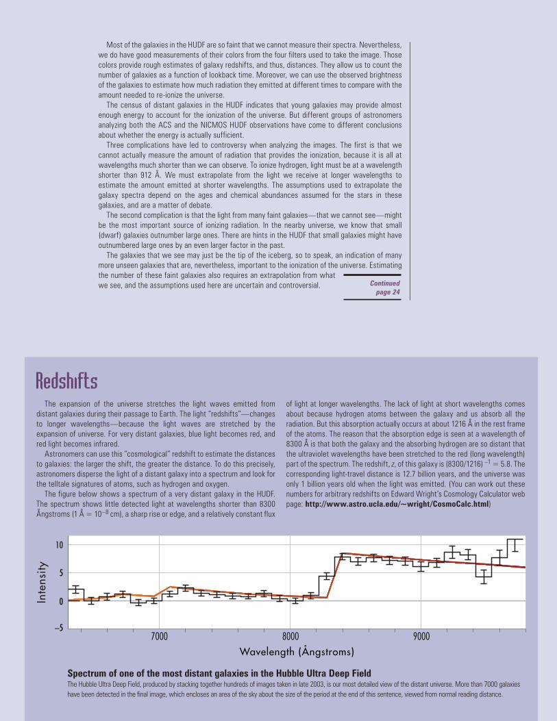
The figure below shows a spectrum of a very distant galaxy in the HUDF. The spectrum shows little detected light at wavelengths shorter than 8300 Ångstroms (1 Å = 10–8 cm), a sharp rise or edge, and a relatively constant flux

of light at longer wavelengths. The lack of light at short wavelengths comes about because hydrogen atoms between the galaxy and us absorb all the radiation. But this absorption actually occurs at about 1216 Å in the rest frame of the atoms. The reason that the absorption edge is seen at a wavelength of 8300 Å is that both the galaxy and the absorbing hydrogen are so distant that the ultraviolet wavelengths have been stretched to the red (long wavelength) part of the spectrum. The redshift, z, of this galaxy is (8300/1216) –1 = 5.8. The corresponding light-travel distance is 12.7 billion years, and the universe was only 1 billion years old when the light was emitted. (You can work out these numbers for arbitrary redshifts on Edward Wright’s Cosmology Calculator web page: http://www.astro.ucla.edu/~wright/CosmoCalc.html)

Wavelength (Ångstroms)7000 8000 9000

Inte

nsity

10

5

0

–5

Spectrum of one of the most distant galaxies in the Hubble Ultra Deep Field The Hubble Ultra Deep Field, produced by stacking together hundreds of images taken in late 2003, is our most detailed view of the distant universe. More than 7000 galaxies have been detected in the final image, which encloses an area of the sky about the size of the period at the end of this sentence, viewed from normal reading distance.

Continuedpage 24

24

HUDFfrom page 23

Imagine trying to tell time from the leaves on a tree. You might guess the time of year from whether the leaves are green or brown, opening or falling. In a temperate climate, you could be sure of the season and might be able to estimate the date to within a month. If you were more scientific, and had a whole forest of trees, you might be able to pin down the date to within a week—or even just a few days—if you understood the soil, weather history, the

unique properties and behavior of each type of tree. So it is also with stars.Stars have chronologies, like trees. They are similarly complex to read, but they yield to science.

As they burn their nuclear fuel over eons, changes in temperature and chemical compositions reflect the passage of time. Further, because at birth stars gather raw material from interstellar space which is detritus from earlier generations of stars, each star bespeaks not only its individual evolution during its lifetime, but also events involving many other stars long past. As we learn to interpret this stellar record, we open and read the history of galaxies—both our own and others.

For the past several years, the Hubble observing proposal solicitation has encouraged “treasury” proposals—proposals to obtain large data sets aimed at an unusually diverse set of scientific questions, or proposals for observations that lay the groundwork for other research. One of these treasury programs, a three-year sequence of spectroscopic observations, is providing a new foundation for our chronology of stars and galaxies.

A spectrograph breaks the light of a star into a highly detailed record of brightness versus wavelength. Chemical elements in the outer layers of stellar gas absorb and emit light at particular wavelengths, corresponding to the internal transitions of the particular atoms making up the star. Thus, spectra reveal a star’s chemical makeup and the temperature of the layer of its atmosphere where most starlight emerges, called the photosphere.

Stellar spectra contain a vast amount of information—a fact that makes them both valuable and difficult to interpret. Conditions in the stellar photosphere are difficult or impossible to reproduce in the laboratory, and the spectra involve millions of atomic transitions. Our knowledge of atoms is based in part on stellar spectra, which means the research is reciprocal. Astrophysicists use the best available laboratory data and theoretical calculations to make a first attempt at matching stellar spectra. Where there are discrepancies, they try to adjust the atomic physics and calculate a new spectrum, making sure the adjustments are still consistent with the laboratory data. Observations of stars of different chemical compositions and temperatures also help ensure consistency.

A final difficulty is that we do not know for sure that the universe was ionized all at once during just a brief period. It could have happened more gradually. In the gradual picture, galaxies would create zones of ionization around them, essentially bubbles of ionized gas in a sea of neutral atoms. As more and more galaxies were born, these zones would grow and overlap like Swiss cheese, eventually merging together completely to eliminate any pockets of neutral atoms. It would be difficult to see this pattern in a single, narrow field such as the Hubble Ultra Deep Field. Detecting such fluctuations will be a challenge for future observations.

A particularly exciting prospect is the possibility of deep observations with the Wide Field Camera 3 (WFC3), a new camera that is ready for installation on Hubble. This camera provides a large field of view at wavelengths longer than the red limit of the ACS. Using the same techniques that have been applied in the HUDF, the camera will allow a search for ionizing sources out to redshifts as high as 10, less than 500 million years after the Big Bang. Based on estimated ages of some of the most distant galaxies in the HUDF, we expect to find at least a few young galaxies at this greater distance. Observations with WFC3 should help reveal how many galaxies started forming in this early era, and whether they provided enough energy to re-ionize the intergalactic gas.

Toward the middle of the next decade, the James Webb Space Telescope will expand the frontier to redshifts as high as 30, giving us the ability to detect still fainter and more distant galaxies when they were forming their very first stars. W

Stellar Chronology Ruth Peterson, peterson@ucolick.org

Ruth Peterson is a research

astronomer af f il iated with

the University of California,

Santa Cruz and Astrophysical

Advances, Incorporated. Her

studies of stars and stellar

clusters range from detailed

studies of a single chemical

element in a single star, to

using vast collections of stars

to determine the ages of

entire galaxies. She is principal

investigator of the Hubble

Treasury program entitled Mid-

Ultraviolet Spectral Templates

for Old Stellar Systems, which

aims to provide the foundation

for more precise estimates

of the ages and star-forming

histories of galaxies.

Continuedpage 27

25

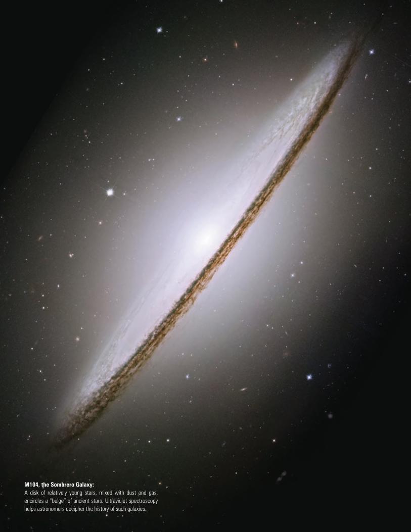
M104, the Sombrero Galaxy: A disk of relatively young stars, mixed with dust and gas, encircles a “bulge” of ancient stars. Ultraviolet spectroscopy helps astronomers decipher the history of such galaxies.

26

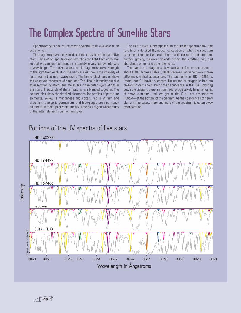
The Complex Spectra of Sun-like StarsSpectroscopy is one of the most powerful tools available to an

astronomer. The diagram shows a tiny portion of the ultraviolet spectra of five

stars. The Hubble spectrograph stretches the light from each star so that we can see the change in intensity in very narrow intervals of wavelength. The horizontal axis in this diagram is the wavelength of the light from each star. The vertical axis shows the intensity of light received at each wavelength. The heavy black curves show the observed spectrum of each star. The dips in intensity are due to absorption by atoms and molecules in the outer layers of gas in the stars. Thousands of these features are blended together. The colored dips show the detailed absorption line profiles of particular elements. Yellow is manganese and cobalt, red is yttrium and zirconium, orange is germanium, and blue/purple are rare heavy elements. In metal-poor stars, the UV is the only region where many of the latter elements can be measured.

The thin curves superimposed on the stellar spectra show the results of a detailed theoretical calculation of what the spectrum is expected to look like, assuming a particular stellar temperature, surface gravity, turbulent velocity within the emitting gas, and abundance of iron and other elements.

The stars in this diagram all have similar surface temperatures—about 6,000 degrees Kelvin (10,000 degrees Fahrenheit)—but have different chemical abundances. The topmost star, HD 140283, is “metal poor.” Heavier elements like carbon or oxygen or iron are present in only about 1% of their abundance in the Sun. Working down the diagram, there are stars with progressively larger amounts of heavy elements, until we get to the Sun—not observed by Hubble—at the bottom of the diagram. As the abundances of heavy elements increases, more and more of the spectrum is eaten away by absorption.

Wavelength in Ångstroms

Inte

nsity

HD 140283

HD 184499

HD 157466

Procyon

SUN - FLUX

3060 3061 3062 3063 3064 3065 3066 3067 3068 3069 3070 3071

1.0.9.8.7.6.5.4.3.2.1.0

Portions of the UV spectra of five stars

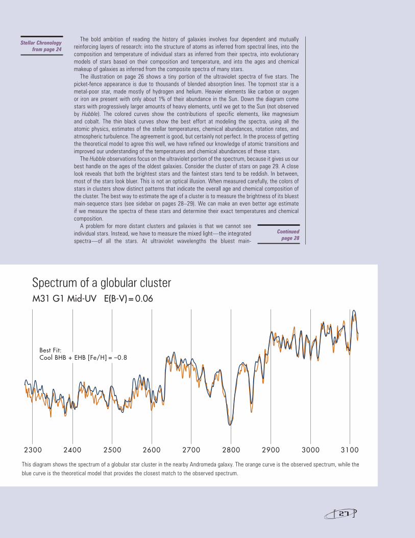
27

2300 2400 2500 2600 2700 2800 2900 3000 3100

M31 G1 Mid-UV E(B-V) = 0.06

Best Fit:Cool BHB + EHB [Fe/H] = –0.8

This diagram shows the spectrum of a globular star cluster in the nearby Andromeda galaxy. The orange curve is the observed spectrum, while the blue curve is the theoretical model that provides the closest match to the observed spectrum.

Spectrum of a globular cluster

The bold ambition of reading the history of galaxies involves four dependent and mutually reinforcing layers of research: into the structure of atoms as inferred from spectral lines, into the composition and temperature of individual stars as inferred from their spectra, into evolutionary models of stars based on their composition and temperature, and into the ages and chemical makeup of galaxies as inferred from the composite spectra of many stars.

The illustration on page 26 shows a tiny portion of the ultraviolet spectra of five stars. The picket-fence appearance is due to thousands of blended absorption lines. The topmost star is a metal-poor star, made mostly of hydrogen and helium. Heavier elements like carbon or oxygen or iron are present with only about 1% of their abundance in the Sun. Down the diagram come stars with progressively larger amounts of heavy elements, until we get to the Sun (not observed by Hubble). The colored curves show the contributions of specific elements, like magnesium and cobalt. The thin black curves show the best effort at modeling the spectra, using all the atomic physics, estimates of the stellar temperatures, chemical abundances, rotation rates, and atmospheric turbulence. The agreement is good, but certainly not perfect. In the process of getting the theoretical model to agree this well, we have refined our knowledge of atomic transitions and improved our understanding of the temperatures and chemical abundances of these stars.

The Hubble observations focus on the ultraviolet portion of the spectrum, because it gives us our best handle on the ages of the oldest galaxies. Consider the cluster of stars on page 29. A close look reveals that both the brightest stars and the faintest stars tend to be reddish. In between, most of the stars look bluer. This is not an optical illusion. When measured carefully, the colors of stars in clusters show distinct patterns that indicate the overall age and chemical composition of the cluster. The best way to estimate the age of a cluster is to measure the brightness of its bluest main-sequence stars (see sidebar on pages 28–29). We can make an even better age estimate if we measure the spectra of these stars and determine their exact temperatures and chemical composition.

A problem for more distant clusters and galaxies is that we cannot see individual stars. Instead, we have to measure the mixed light—the integrated spectra—of all the stars. At ultraviolet wavelengths the bluest main-

Continuedpage 28

Stellar Chronology from page 24

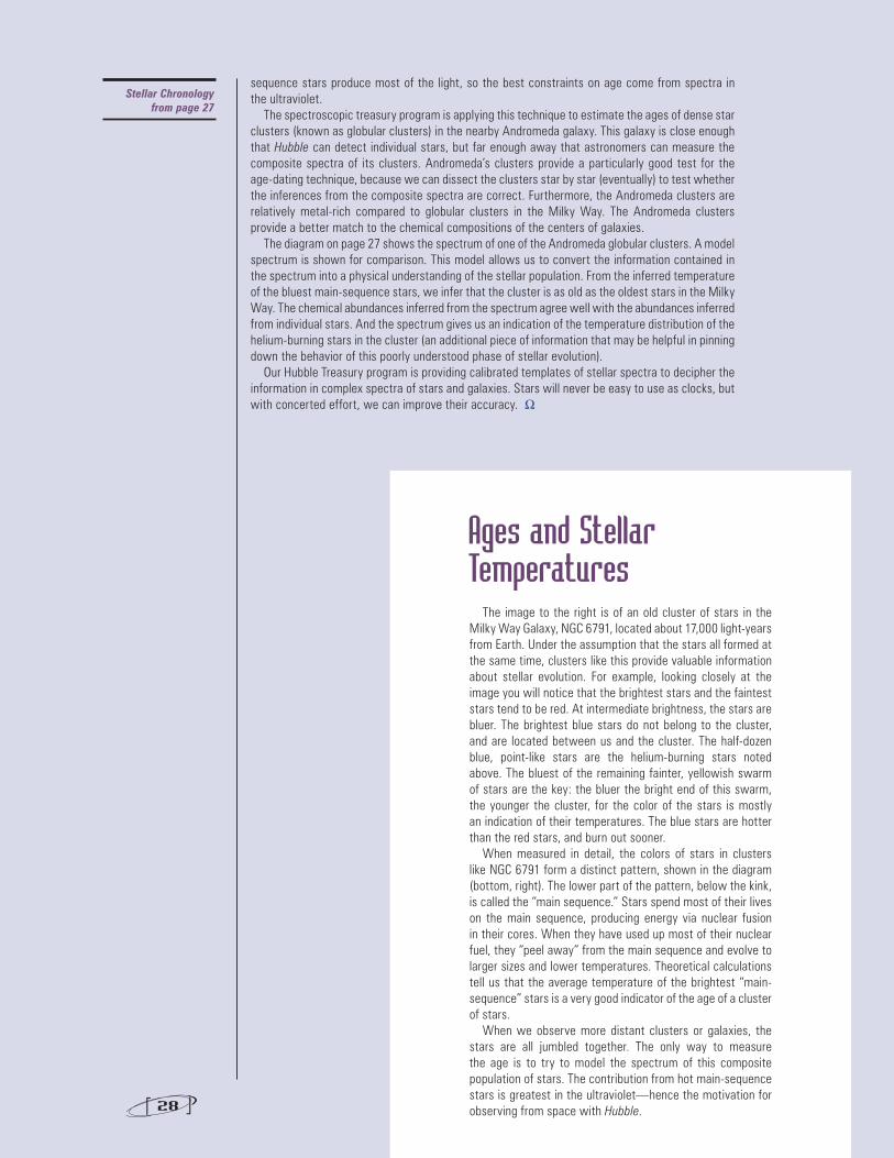
28

Ages and Stellar Temperatures

The image to the right is of an old cluster of stars in the Milky Way Galaxy, NGC 6791, located about 17,000 light-years from Earth. Under the assumption that the stars all formed at the same time, clusters like this provide valuable information about stellar evolution. For example, looking closely at the image you will notice that the brightest stars and the faintest stars tend to be red. At intermediate brightness, the stars are bluer. The brightest blue stars do not belong to the cluster, and are located between us and the cluster. The half-dozen blue, point-like stars are the helium-burning stars noted above. The bluest of the remaining fainter, yellowish swarm of stars are the key: the bluer the bright end of this swarm, the younger the cluster, for the color of the stars is mostly an indication of their temperatures. The blue stars are hotter than the red stars, and burn out sooner.

When measured in detail, the colors of stars in clusters like NGC 6791 form a distinct pattern, shown in the diagram (bottom, right). The lower part of the pattern, below the kink, is called the “main sequence.” Stars spend most of their lives on the main sequence, producing energy via nuclear fusion in their cores. When they have used up most of their nuclear fuel, they “peel away” from the main sequence and evolve to larger sizes and lower temperatures. Theoretical calculations tell us that the average temperature of the brightest “main-sequence” stars is a very good indicator of the age of a cluster of stars.

When we observe more distant clusters or galaxies, the stars are all jumbled together. The only way to measure the age is to try to model the spectrum of this composite population of stars. The contribution from hot main-sequence stars is greatest in the ultraviolet—hence the motivation for observing from space with Hubble.

sequence stars produce most of the light, so the best constraints on age come from spectra in the ultraviolet.

The spectroscopic treasury program is applying this technique to estimate the ages of dense star clusters (known as globular clusters) in the nearby Andromeda galaxy. This galaxy is close enough that Hubble can detect individual stars, but far enough away that astronomers can measure the composite spectra of its clusters. Andromeda’s clusters provide a particularly good test for the age-dating technique, because we can dissect the clusters star by star (eventually) to test whether the inferences from the composite spectra are correct. Furthermore, the Andromeda clusters are relatively metal-rich compared to globular clusters in the Milky Way. The Andromeda clusters provide a better match to the chemical compositions of the centers of galaxies.

The diagram on page 27 shows the spectrum of one of the Andromeda globular clusters. A model spectrum is shown for comparison. This model allows us to convert the information contained in the spectrum into a physical understanding of the stellar population. From the inferred temperature of the bluest main-sequence stars, we infer that the cluster is as old as the oldest stars in the Milky Way. The chemical abundances inferred from the spectrum agree well with the abundances inferred from individual stars. And the spectrum gives us an indication of the temperature distribution of the helium-burning stars in the cluster (an additional piece of information that may be helpful in pinning down the behavior of this poorly understood phase of stellar evolution).

Our Hubble Treasury program is providing calibrated templates of stellar spectra to decipher the information in complex spectra of stars and galaxies. Stars will never be easy to use as clocks, but with concerted effort, we can improve their accuracy. W

Stellar Chronologyfrom page 27

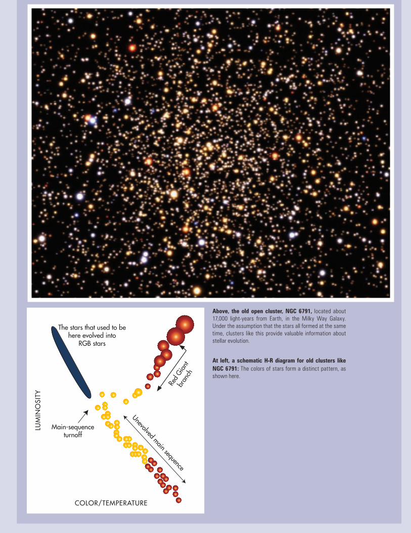
COLOR/TEMPERATURE

The stars that used to be here evolved into

RGB stars

Red

Giant

bran

ch

Unevolved main sequence

Main-sequence turnoff

LUM

INO

SITY

Above, the old open cluster, NGC 6791, located about 17,000 light-years from Earth, in the Milky Way Galaxy. Under the assumption that the stars all formed at the same time, clusters like this provide valuable information about stellar evolution.

At left, a schematic H-R diagram for old clusters like NGC 6791: The colors of stars form a distinct pattern, as shown here.

Hubble IllumInates “Dorian Gray” Galaxyhttp://hubblesite.org/newscenter/archive/releases/2007/35/Image Credit: NASA, ESA, and A. Aloisi (Space Telescope Science Institute and European Space Agency, Baltimore, Md.)

N ASA’s Hubble Space Telescope quashed the possibility that what was previously believed to be a toddler galaxy in the nearby universe may actually be considered an adult. Called I Zwicky 18, this galaxy has a youthful appearance that resembles galaxies typically found only in the early universe. Hubble has now found faint, older stars within this galaxy, suggesting that the galaxy may have formed at the same time as most other galaxies. For the first

time, Hubble data also allowed astronomers to identify Cepheid variable stars in I Zwicky 18. These flashing stellar mile-markers were used to determine that I Zwicky 18 is 59 million light-years from Earth, almost 10 million light-years more distant than previously believed.

The Space Telescope–European Coordinating Facility publishes a newsletter which, although aimed principally at European Space Telescope users, contains articles of general interest to the HST community. If you wish to be included in the mailing list, please contact the editor

and state your affiliation and specific involvement in the Space Telescope Project.

Richard Hook (Editor)

Space Telescope–European Coordinating FacilityKarl Schwarzschild Str. 2D-85748 Garching bei MünchenGermanyE-Mail: rhook@eso.org

ST-ECF Newsletter

An Atlas of Interacting Galaxies

A stronomy textbooks typically present galaxies as staid, solitary, and majestic island worlds of glittering stars. But galaxies have a dynamical side. They have close encounters that sometimes end in grand mergers and overflowing sites of new star birth as the colliding

galaxies morph into wondrous new shapes. In celebration of the Hubble Space Telescope’s 18th launch anniversary, 59 views of colliding galaxies—constituting the largest collection of Hubble images ever—were released to the public. This new Hubble atlas dramatically illustrates how galaxy collisions produce a remarkable variety of intricate structures in never-before-seen detail.

http://hubblesite.org/newscenter/archive/releases/2008/16/

Image Credit: NASA, ESA, the Hubble Heritage (STScI/AURA)-ESA/Hubble Collaboration, and A. Evans (University of Virginia, Charlottesville/NRAO/Stony Brook University)

The Institute’s website is: http://www.stsci.eduAssistance is available at help@stsci.edu or 800-544-8125. International callers can use 1-410-338-1082.

For current Hubble users, program information is available at:http://presto.stsci.edu/public/propinfo.html.The current members of the Space Telescope Users Committee (STUC) are:

Pat McCarthy (chair), Carnegie Observatories, pmc2@ociw.edu

The Space Telescope Science Institute Newsletter is edited by Robert Brown, rbrown@stsci.edu, who invites comments and suggestions.

Technical Lead: Christian Lallo, clallo@stsci.eduContents Manager: Sharon Toolan, toolan@stsci.eduDesign: Kathy Cordes, cordes@stsci.edu

To record a change of address or to request receipt of the Newsletter, please send a message to address-change@stsci.edu.

Contact STScI

Martin Barstow, U. of Leicester

Peter Garnavich, U. of Notre Dame

Jim Green, U. of Colorado

Jean-Paul Kneib, OAMP

David Koo, UCSC

Lori Lubin, UCD

Mario Mateo, U. of Michigan

Phil Nicholson, Cornell U.

Robert O’Connell, U. of Virginia

Alvio Renzini, INAF

Abi Saha, NOAO

Tommaso Treu, UCSB

Marianne Vestergaard, U. of Arizona

31

IN OUR NEXT ISSUE:

Calendar

3700 San Martin Drive, Baltimore, Maryland 21218

NON PROFIT U.S. POSTAGE

PAIDPERMIT NO. 8928BALTIMORE, MD

STSc

I N-0

1-08

Contents:Synergy Between Webb and Hubble. . . . . . . . . . . . . . . . . . 1ACS Report . . . . . . . . . . . . . . . . . . . . . . . . . . . . . . . . . . . . . 3NICMOS: Improving Science by Removing Bright-Earth Persistence . . . . . . . . . . . . . . . . 4STIS Update . . . . . . . . . . . . . . . . . . . . . . . . . . . . . . . . . . . . 5Improving Hubble’s Pointing and Astrometry. . . . . . . . . . . . 7WFC3 Status. . . . . . . . . . . . . . . . . . . . . . . . . . . . . . . . . . . . 9COS Status . . . . . . . . . . . . . . . . . . . . . . . . . . . . . . . . . . . . 11Testing the MIRI Verification Model. . . . . . . . . . . . . . . . . . 12Institute Honors John Bahcall . . . . . . . . . . . . . . . . . . . . . . 14Introducing John Mather to the Science Operations Center . . . . . . . . . . . . . . . . . . 15Plumbing the Depth of the Hubble Ultra Deep Field . . . . . 16The Hubble Ultra Deep Field . . . . . . . . . . . . . . . . . . . . . . . 20Stellar Chronology . . . . . . . . . . . . . . . . . . . . . . . . . . . . . . . 24

Contact STScI . . . . . . . . . . . . . . . . . . . . . . . . . . . . . . . . . . 31Calendar . . . . . . . . . . . . . . . . . . . . . . . . . . . . . . . . . . . . . . 32

May Symposium, A Decade of Dark Energy, http://www.stsci.edu/institute/conference/spring2008 . . . . . . . . 5–8 May 2008HST Cycle 17 Panels and TAC meeting . . . . . . . . . . . . . . . . . . . . . . . . . . 12–16 May 2008MAST Senior Review proposal deadline . . . . . . . . . . . . . . . . . . . . . . . . . . . . 16 May 2008Youth for Astronomy & Engineering (YAE) Program, Women’s Science Forum for Middle Schools (STScI Auditorium) . . . . . . . . . . . . . . . . . . . . . 17 May 2008 IIVC . . . . . . . . . . . . . . . . . . . . . . . . . . . . . . . . . . . . . . . . . . . . . . . . . . 19–20 May 2008HST Cycle 17 TAC results released . . . . . . . . . . . . . . . . . . . . . . . . . . . . . . . . 28 May 2008Youth for Astronomy & Engineering (YAE) Program, Women’s Science Forum for Middle Schools (STScI Auditorium) . . . . . . . . . . . . . . . . . . . . . 31 May 2008 AAS meeting (St. Louis) . . . . . . . . . . . . . . . . . . . . . . . . . . . . . . . . . . . . . . . 1–5 June 2008STIC (Garching) . . . . . . . . . . . . . . . . . . . . . . . . . . . . . . . . . . . . . . . . . . . . 17–18 June 2008NASA Data Centers’ Senior Review . . . . . . . . . . . . . . . . . . . . . . . . . . . . 17–19 June 2008SPIE, Astronomical Instrumentation (Marseille) . . . . . . . . . . . . . . . . . . . 23–28 June 2008HST Cycle 17 Phase II deadline. . . . . . . . . . . . . . . . . . . . . . . . . . . . . . . . . . . . .3 July 2008JWST SWG (Noordwijk) . . . . . . . . . . . . . . . . . . . . . . . . . . . . . . . . . . . . . . .9–10 July 2008STS 125 launch (KSC). . . . . . . . . . . . . . . . . . . . . . . . . . . . . . . . . . . . . . . . .8 October 2008STUC meeting (STScI). . . . . . . . . . . . . . . . . . . . . . . . . . . . . . . . . . .13–14 November 2008