Synergy between Object Recognition and Image Segmentation Using the Expectation-Maximization Algorithm

Synergy between Object Recognition andImage Segmentation Using

the Expectation-Maximization AlgorithmIasonas Kokkinos, Member, IEEE, and Petros Maragos, Fellow, IEEE

Abstract—In this work, we formulate the interaction between image segmentation and object recognition in the framework of the

Expectation-Maximization (EM) algorithm. We consider segmentation as the assignment of image observations to object hypotheses

and phrase it as the E-step, while the M-step amounts to fitting the object models to the observations. These two tasks are performed

iteratively, thereby simultaneously segmenting an image and reconstructing it in terms of objects. We model objects using Active

Appearance Models (AAMs) as they capture both shape and appearance variation. During the E-step, the fidelity of the AAM

predictions to the image is used to decide about assigning observations to the object. For this, we propose two top-down segmentation

algorithms. The first starts with an oversegmentation of the image and then softly assigns image segments to objects, as in the

common setting of EM. The second uses curve evolution to minimize a criterion derived from the variational interpretation of EM and

introduces AAMs as shape priors. For the M-step, we derive AAM fitting equations that accommodate segmentation information,

thereby allowing for the automated treatment of occlusions. Apart from top-down segmentation results, we provide systematic

experiments on object detection that validate the merits of our joint segmentation and recognition approach.

Index Terms—Image segmentation, object recognition, Expectation Maximization, Active Appearance Models, curve evolution,

top-down segmentation, generative models.

Ç

1 INTRODUCTION

THE bottom-up approach to vision [28] has considered theinteraction between image segmentation and object

detection in the scenario where segmentation groupscoherent image areas that are then used to assemble anddetect objects. Due to its simplicity, this approach has beenwidely adopted, but there is a growing understanding thatthe cooperation (synergy) of these two processes canenhance performance.

Models that integrate the bottom-up and top-downstreams of information were proposed during the previousdecade by researchers in cognitive psychology, biologicalvision, and neural networks [12], [31], [33], [41], [48], wherethe primary concerns have been at the architectural andfunctional level. In this decade, the first concrete computervision approaches to the problem [7], [54] have inspired ahost of more recent systems [6], [15], [21], [24], [25], [27],[32], [45], [51], [52], pursuing the exploitation of this idea.

Several of these works have been inspired by theanalysis-by-synthesis framework of Pattern Theory [17],[34], [45]. In this setting, a set of probabilistic generativemodels is used to synthesize the observed image and the

analysis task amounts to estimating the model parameters.This approach can simultaneously regularize low-leveltasks using model-based information and validate objecthypotheses based on how well they predict the image.

In our work, we use Active Appearance Models (AAMs)as generative models and address the problem of jointlydetecting and segmenting objects in images. Our maincontribution, preliminarily presented in [21], is phrasingthis task in the framework of the Expectation-Maximization(EM) algorithm [13]. Specifically, we view image segmenta-tion as the E-step, where image observations are assigned tothe object hypotheses. Model fitting is seen as the M-step,where the parameters related to each object hypothesis areestimated so as to optimally explain the image observationsassigned to it. Segmentation and fitting proceed iteratively;since we are working in the framework of EM, this isguaranteed to converge to a locally optimal solution.

To make the combination of different approachestractable, we build on the variational interpretation of EM;this phrases EM as the iterative maximization of a criterionthat is a lower bound on the observation likelihood.Specifically, we consider two alternative approaches forthe implementation of the E-step; the first initially uses anoff-the-shelf oversegmentation algorithm and then assignsthe formed segments to objects. The second uses a curve-evolution-based E-step that combines AAMs with varia-tional image segmentation. Both approaches can be seen asoptimizing the criterion used in the variational interpreta-tion of EM. Further, we combine AAM fitting and imagesegmentation based on this criterion. We derive modifiedfitting equations that incorporate segmentation information,thereby automatically dealing with occlusions.

1486 IEEE TRANSACTIONS ON PATTERN ANALYSIS AND MACHINE INTELLIGENCE, VOL. 31, NO. 8, AUGUST 2009

. I. Kokkinos is with the Department of Applied Mathematics, Ecole Centralede Paris, Grande Voie des Vignes, 92295 Chatenay-Malabry, France, andEquipe Galen, INRIA-Saclay. E-mail: [email protected].

. P. Maragos is with the School of Electrical and Computer Engineering,National Technical University of Athens, Zografou Campus, 15773,Athens, Greece. E-mail: [email protected].

Manuscript received 6 May 2007; revised 14 Jan. 2008; accepted 30 Apr.2008; published online 5 June 2008.Recommended for acceptance by S.-C. Zhu.For information on obtaining reprints of this article, please send e-mail to:[email protected], and reference IEEECS Log NumberTPAMI-2007-05-0262.Digital Object Identifier no. 10.1109/TPAMI.2008.158.

0162-8828/09/$25.00 � 2009 IEEE Published by the IEEE Computer Society

Finally, we provide systematic object detection resultsfor faces and cars, demonstrating the merit of this jointsegmentation and recognition approach.

Paper outline. In Section 2, we introduce the basicnotions of EM and give an overview of our approach.Section 3 presents the generative models we use andformulates the variational criterion optimized by EM. Wepresent the two considered approaches for the E-step inSection 4 and derive the M-step for AAMs in Section 5.Experimental results are provided in Section 6, whileSection 7 places our work in the context of existingapproaches; technical issues are addressed in the Appendix,which can be found in the Computer Society Digital Libraryat http://doi.ieeecomputersociety.org/TPAMI.2008.158.

2 EM APPROACH TO SYNERGY

Our work builds on the approach of generative models tosimultaneously address the segmentation and recognitionproblems. For the purpose of segmentation, we use thefidelity of the generative model predictions to the image inorder to decide which part of the image a model shouldoccupy. Regarding recognition, each object hypothesis isvalidated based on the image area assigned to the object, aswell as the estimated model parameters, which indicate thefamiliarity of the object appearance.

This yields, however, an intertwined problem: On onehand, knowing the area occupied by an object is needed forthe estimation of the model parameters and, on the otherhand, the model synthesis is used to assign observations tothe model. Since neither is known in advance, we cannotaddress each problem separately. We view this problem asan instance of the broader problem of parameter estimationwith missing data: In our case, the missing data are theassignments of observations to models. A well-known toolfor addressing such problems is the EM algorithm [13],which we now briefly describe for the problem of parameterestimation for a mixture distribution [5] before presentinghow it applies to our approach.

2.1 EM Algorithm and Variational Interpretation

Consider generating an observation In by first choosing oneout of K parametric distributions, with prior probability �k,and then drawing a sample from that distribution withprobability P ðInj�kÞ. EM addresses the task of estimatingthe parameter set A ¼ fA1; . . . ;Akg, Ak ¼ ð�k; �kÞ, whichoptimally explains a set of observations I ¼ fI1; . . . ; INggenerated this way.

The missing data are the identities of the distributionsused to generate each observation; these are representedwith the binary hidden variable vectors zn ¼ ½zn;1; . . . ; zn;K �T .zn corresponds to the nth observation and its uniquenonzero element indicates the component used to generateIn. By summing over the unknown hidden variablesZ ¼ fz1; . . . ; zng, we can express the likelihood of theobservations given the parameter set:

logP ðIjAÞ ¼XNn¼1

logP ðInjAÞ ¼XNn¼1

logXzn

P ðIn; znjAÞ: ð1Þ

We can write the last summand as

P ðIn; znjAÞ ¼ P ðInjzn;AÞP ðznjAÞ ¼YKk¼1

�kP ðInj�kÞ½ �zn;k : ð2Þ

Finding the optimal estimate A� is intractable, since the

summation over zn appears inside the logarithm in (1).

However, for a given Z, one can write the full observation log

likelihood:

logP ðI;ZjAÞ ¼Xn

Xk

zn;k log �kP ðInj�kÞð Þ: ð3Þ

The parameters in this expression can be directly estimated

since the summation appears outside the logarithm.The EM algorithm exploits this by introducing the

expectation of (3) with respect to the posterior distribution

of zn;k. Denoting by zn;k the vector zn that assigns

observation n to the kth mixture, i.e., has zn;k ¼ 1, we write

the EM algorithm as iterating the following steps:

. E-step. Derive the posterior of z conditioned onthe previous parameter estimates, A�, and theobservations:

En;k � P ðzn;kjIn;A�Þ ¼��kP Inj��k

� �P

j ��jP Inj��j� � ; ð4Þ

and form the expected value of the log likelihood

under this probability mass function:

logP I;ZjA�ð Þh iE¼Xn

Xk

En;k log �kP ðInj�kÞð Þ: ð5Þ

. M-step. Maximize the expected log likelihood withrespect to the distribution parameters:

��k ¼P

n En;k

N; ��k ¼ arg max

Xn

En;k logP ðInj�kÞ:

ð6Þ

Intuitively, in the E-step, the unobserved binary variables in

(3) are replaced with an estimate of each mixture’s

“responsibility” for the observations, which is then used

to decouple parameter estimation in the M-step. This

consistently increases the likelihood [13] and converges to

a local maximum of (1).EM can also be seen as a variational inference algorithm

[18] along the lines of [35]. There, it is shown to iteratively

maximize a lower bound on the observation likelihood:

logP ðIjAÞ �LBðI;Q;AÞ;

LBðI;Q;AÞ ¼X

Z

QðZÞ logP ðIjZ;AÞP ðZjAÞ

logQðZÞ :ð7Þ

The bound LB is expressed in terms of Q, an unknown

distribution on the hidden variables Z, and the parameter

set A. The form in (7) is derived from Jensen’s inequality.

Typically, Q is chosen from a manageable family of

distributions; for example, by choosing a factorizable

distribution Q ¼QQnðznÞ, computations become tractable

since the summations in (7) break over n.The individual distribution QnðznÞ determines the prob-

ability of assigning the nth observation to one of the

K components. To make the relation with (4) clear, we use

KOKKINOS AND MARAGOS: SYNERGY BETWEEN OBJECT RECOGNITION AND IMAGE SEGMENTATION USING THE EXPECTATION... 1487

Qn;k to denote the probability of zn;k. By breaking theproduct in the logarithm, we can thus write (7) as

LBðI;Q;AÞ ¼Xn;k

Qn;k½logP ðInjAkÞ

þ logP ðzn;kjAkÞ � logQn;k�:ð8Þ

Maximizing the bound in (8) with respect to Q subject to theconstraint that

Pk Qn;k ¼ 1, 8n, leads to Qn;k ¼ En;k. There-

fore, the variational approach to EM interprets the E-step asa maximization with respect to Q.

Apart from providing a common criterion for the twosegmentation algorithms used subsequently, this formula-tion makes several expressions easier. For example, bybreaking the product in (7) and keeping the termP

Z QðZÞ logP ðZjAÞ, we have a quantity that captures priorinformation about assignments. For mixture modeling, thissimply amounts to the expression

Pn

Pk Qn;k log�k, which

favors assignments to clusters with larger mixing weights.In image segmentation, however, there are other forms ofpriors, such as small length of the boundaries betweenregions, or object-specific priors, capturing the shapeproperties of the object. We will express all of these interms of QðZÞ logP ðZjAÞ.

2.2 Application to Synergy

In the mixture modeling problem, the hidden variablevectors provide an assignment of each observation to aspecific mixture component. The analogy with our problemcomes by seeing the object models as the mixturecomponents and the hidden variables as providing theimage segmentation.

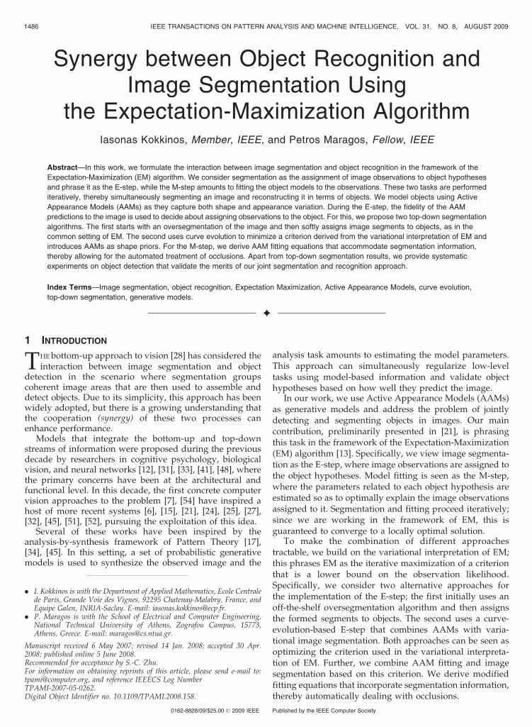
We apply the EM algorithm to our problem by treatingsegmentation as the E-step and model fitting as the M-step,as shown in Fig. 1. In the E-step, we determine theresponsibility of the object model for image observationsand, in the M-step, we estimate the model parameters so asto optimally explain the data that it has occupied.Intuitively, we consider segmentation as determining awindow through which the object is seen, with binaryhidden variables determining whether the object is visible

or not. Top-down segmentation decides where it is best toopen this window, while model fitting focuses on the objectparts seen through it.

Illustrating this idea, Fig. 2 shows the result of iteratingthe E- and M-steps for a toy example: Starting from alocation in the image proposed by a front-end detectionsystem, the synthesis and segmentation gradually improve,converging to a solution that models a region of the imagein terms of an object. The assignment of observations to amodel and the estimation of the model parameters proceedin a gradual relaxation-type fashion until convergence.

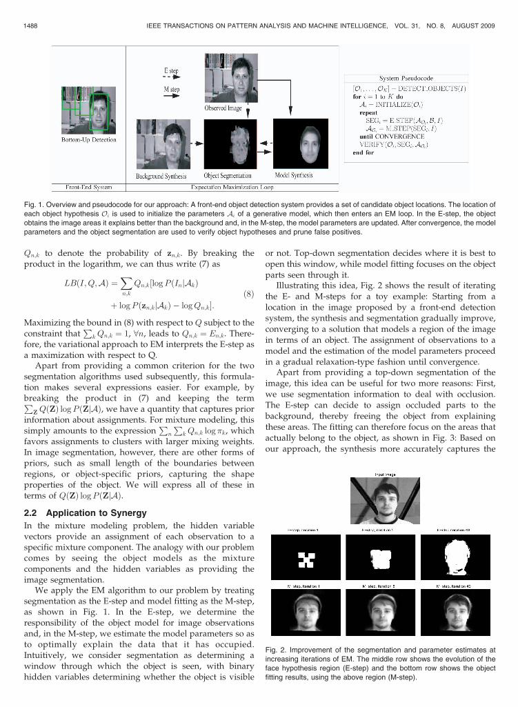
Apart from providing a top-down segmentation of theimage, this idea can be useful for two more reasons: First,we use segmentation information to deal with occlusion.The E-step can decide to assign occluded parts to thebackground, thereby freeing the object from explainingthese areas. The fitting can therefore focus on the areas thatactually belong to the object, as shown in Fig. 3: Based onour approach, the synthesis more accurately captures the


Fig. 1. Overview and pseudocode for our approach: A front-end object detection system provides a set of candidate object locations. The location of

each object hypothesis Oi is used to initialize the parameters Ai of a generative model, which then enters an EM loop. In the E-step, the object

obtains the image areas it explains better than the background and, in the M-step, the model parameters are updated. After convergence, the model

parameters and the object segmentation are used to verify object hypotheses and prune false positives.

Fig. 2. Improvement of the segmentation and parameter estimates at

increasing iterations of EM. The middle row shows the evolution of the

face hypothesis region (E-step) and the bottom row shows the object

fitting results, using the above region (M-step).

intensity pattern of the face and gives reasonable predic-tions in the part that has been occluded. We address this

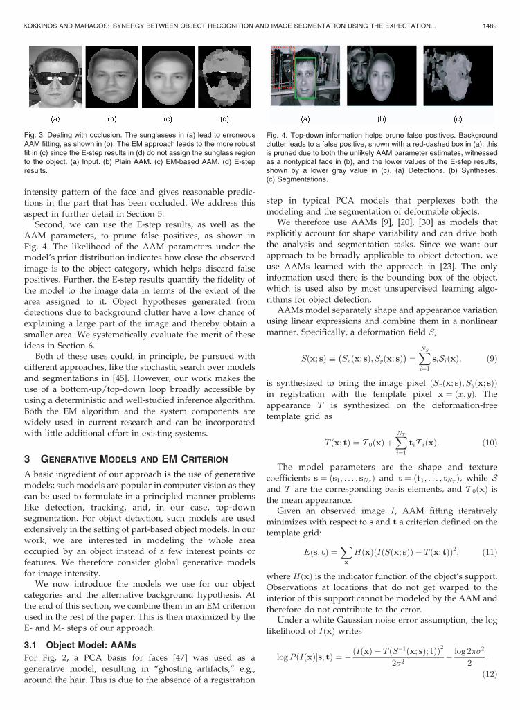
aspect in further detail in Section 5.Second, we can use the E-step results, as well as the

AAM parameters, to prune false positives, as shown in

Fig. 4. The likelihood of the AAM parameters under the

model’s prior distribution indicates how close the observedimage is to the object category, which helps discard false

positives. Further, the E-step results quantify the fidelity of

the model to the image data in terms of the extent of the

area assigned to it. Object hypotheses generated fromdetections due to background clutter have a low chance of

explaining a large part of the image and thereby obtain a

smaller area. We systematically evaluate the merit of these

ideas in Section 6.Both of these uses could, in principle, be pursued with

different approaches, like the stochastic search over models

and segmentations in [45]. However, our work makes the

use of a bottom-up/top-down loop broadly accessible by

using a deterministic and well-studied inference algorithm.

Both the EM algorithm and the system components arewidely used in current research and can be incorporated

with little additional effort in existing systems.

3 GENERATIVE MODELS AND EM CRITERION

A basic ingredient of our approach is the use of generative

models; such models are popular in computer vision as they

can be used to formulate in a principled manner problems

like detection, tracking, and, in our case, top-downsegmentation. For object detection, such models are used

extensively in the setting of part-based object models. In our

work, we are interested in modeling the whole area

occupied by an object instead of a few interest points orfeatures. We therefore consider global generative models

for image intensity.We now introduce the models we use for our object

categories and the alternative background hypothesis. At

the end of this section, we combine them in an EM criterion

used in the rest of the paper. This is then maximized by theE- and M- steps of our approach.

3.1 Object Model: AAMs

For Fig. 2, a PCA basis for faces [47] was used as a

generative model, resulting in “ghosting artifacts,” e.g.,

around the hair. This is due to the absence of a registration

step in typical PCA models that perplexes both the

modeling and the segmentation of deformable objects.We therefore use AAMs [9], [20], [30] as models that

explicitly account for shape variability and can drive both

the analysis and segmentation tasks. Since we want our

approach to be broadly applicable to object detection, we

use AAMs learned with the approach in [23]. The only

information used there is the bounding box of the object,

which is used also by most unsupervised learning algo-

rithms for object detection.AAMs model separately shape and appearance variation

using linear expressions and combine them in a nonlinear

manner. Specifically, a deformation field S,

Sðx; sÞ � Sxðx; sÞ; Syðx; sÞ� �

¼XNS

i¼1

siSiðxÞ; ð9Þ

is synthesized to bring the image pixel ðSxðx; sÞ; Syðx; sÞÞin registration with the template pixel x ¼ ðx; yÞ. The

appearance T is synthesized on the deformation-free

template grid as

T ðx; tÞ ¼ T 0ðxÞ þXNTi¼1

tiT iðxÞ: ð10Þ

The model parameters are the shape and texture

coefficients s ¼ ðs1; . . . ; sNS Þ and t ¼ ðt1; . . . ; tNT Þ, while Sand T are the corresponding basis elements, and T 0ðxÞ is

the mean appearance.Given an observed image I, AAM fitting iteratively

minimizes with respect to s and t a criterion defined on the

template grid:

Eðs; tÞ ¼X

x

HðxÞ I Sðx; sÞð Þ � T ðx; tÞð Þ2; ð11Þ

where HðxÞ is the indicator function of the object’s support.

Observations at locations that do not get warped to the

interior of this support cannot be modeled by the AAM and

therefore do not contribute to the error.Under a white Gaussian noise error assumption, the log

likelihood of IðxÞ writes

logP IðxÞjs; tð Þ ¼ � IðxÞ � T S�1ðx; sð Þ; tÞð Þ2

2�2� log 2��2

2:

ð12Þ


Fig. 3. Dealing with occlusion. The sunglasses in (a) lead to erroneousAAM fitting, as shown in (b). The EM approach leads to the more robustfit in (c) since the E-step results in (d) do not assign the sunglass regionto the object. (a) Input. (b) Plain AAM. (c) EM-based AAM. (d) E-stepresults.

Fig. 4. Top-down information helps prune false positives. Backgroundclutter leads to a false positive, shown with a red-dashed box in (a); thisis pruned due to both the unlikely AAM parameter estimates, witnessedas a nontypical face in (b), and the lower values of the E-step results,shown by a lower gray value in (c). (a) Detections. (b) Syntheses.(c) Segmentations.

Here, S�1 fetches from the template coordinate system theprediction T ðS�1ðx; sÞ; tÞ corresponding to the observedvalue IðxÞ and, as above, this equation holds only ifHðS�1ðx; sÞÞ ¼ 1, namely, if x can be explained by the AAM.

If the magnification or shrinking of the template point xis negligible, we have P ðIjs; tÞ / expð�Eðs; tÞ=ð2�2ÞÞ, whichinterprets AAM fitting as providing a Maximum-Like-lihood parameter estimate. Further, we can performMaximum-A-Posterior estimation by introducing a quad-ratic penalty on model parameters in (11), which equals thelog-likelihood of the parameters under a Gaussian priordistribution.

3.2 Background Model: Piecewise Constant Image

To determine the assignment of observations to the object,we need a background model as an alternative to competewith. There are several ways to build a background model,depending on the accuracy required from it. At thesimplicity extreme, in Fig. 2, we use a nonparametricdistribution for the image intensity that is estimated usingthe whole image domain. However, for images withcomplex background, this distribution becomes loose andthe object model may be better even around false positives.The more complex full-blown generative approach in [45],[46] pursues the interpretation of the whole image, so thereis no generic background model. Practically, for the jointsegmentation and detection task, this could be superfluous:As we show in the experimental results, a simple back-ground model can both discard false positives and excludeoccluded areas from model fitting.

The approach we take lies between these two cases. Weconsider that the background model is built by a set ofregions, within which the image has constant intensity; thisis the broadly used piecewise-constant image model. Weassume that, within each region r, the constant value iscorrupted by white Gaussian noise and we estimate theparameters ð�r; �rÞ from the mean and standard deviationof the region’s image intensities. These, together with theprior probability �Br of assigning an observation to theregion, form the parameter set for background region r:ABr ¼ ð�r; �r; �BrÞ.

We can combine all submodels in a single backgroundhypothesis B, under which the likelihood of IðxÞ writes

P IðxÞjABð Þ ¼YRr¼1

P IðxÞjABrð Þ½ �HrðxÞ

¼N �i � IðxÞ; �ið Þ;ð13Þ

where AB ¼ ðAB1; . . . ;ABRÞ, HrðxÞ is the support indicator

for the rth region, and i is the index of the region thatcontains x, i.e., HiðxÞ ¼ 1. Implicitly, in (13), we assume that�Br does not depend on r and condition on IðxÞ belongingto the background; otherwise, a �Bi term would benecessary. This is an expression we will use in the followingwhen convenient.

3.3 EM Criterion for Object versus BackgroundSegmentation

We now build a lower bound on the likelihood of the imageobservations under the mixture of the object and backgroundmodels. For the sake of simplicity, we formulate it for the case

of jointly segmenting and analyzing a single object; thegeneralization to multiple objects is straightforward.

We split the bound in (8) into object and background-related terms. Since our models are formulated in thecontinuous domain but EM considers a discrete set ofobservations, we denote below with xn the image coordi-nate corresponding to observation index n.

We first consider the part of the EM bound in (8) thatinvolves the object hypothesis, O. This can be expressed interms of the column of Qn;k that relates to O, QO, and theobject parameters AO ¼ ðs; t; �OÞ that include the AAMparameters s and t and the prior probability �O of assigningan observation to the object if it falls within its support.Using these, we write the related part of the bound as

LBðI;QO;AOÞ ¼Xn

Qn;O logP ðInjAOÞ þ logP ðzn;OjAOÞ� �

:

ð14Þ

Here, P ðInjAOÞ ¼ P ðIðxnÞjs; tÞ is the observation likelihoodunder the appearance model of (12) and zn;O is the hiddenvariable vector that assigns the observationn to hypothesisO.

The term P ðzn;OjAOÞ equals the prior probability of zn;Ounder the AAM model and constrains the AAM to onlymodel observations in the template interior. Specifically, wehave

P ðzn;OjAOÞ ¼ H S�1ðxn; sÞ� �

�O: ð15Þ

In words, hypothesis O can take hold of observation n onlyif S�1 brings it inside the object’s interior. In that case, theprior probability of obtaining it is �O. This brings shapeinformation directly into the segmentation without introdu-cing additional terms to a segmentation criterion as is done,e.g., in [11], [43]. We therefore see AAMs as providing anatural means to introduce shape-related information in thesegmentation.

For the background model, we adopt the mixture model-ing approach described in the previous section and write

LBðI;QB;ABÞ ¼Xn;r

Qn;Br ½logP InjABrð Þ

þ logP zn;Br jABr� �

�:ð16Þ

As in (14), QB are the columns of Qn;k related to thebackground hypotheses and AB are the correspondingparameters. The first summand is the likelihood of theobservations under the rth background submodel. Thesecond summand is a prior distribution over the assignmentsthat we use to balance the complexity of the foreground andbackground models. Specifically, the AAM often has a largerreconstruction error than the background model since itexplains a heterogeneous set of observations with a varyingset of intensities. Instead, the background regions aredetermined using bottom-up cues and have almost constantintensity, thereby making it easier to model their interiors. Wetherefore assign observations to the object model more easilyby setting P ðzn;Br jABrÞ ¼ �Br to a low value; this gives riselater to “MDL” or “balloon” terms.

We combine these two terms with a scaled version of theentropy-related term of (7) and obtain the following lowerbound on the log likelihood of the data:


LBðI;Q;AÞ ¼Xn

Xh2fO;B1;...;Brg

Qn;h

�logP ðInjAhÞ

þ logP ðzn;hjAhÞ �1

�logQn;h

�;

ð17Þ

where Q ¼ fQO; QBg and A ¼ fAO;ABg. The last summandfavors high-entropy distributions and leads to soft assign-ments. Since �

Pn;h Qn;h logQn;h � 0, for all � � 1, we have

a lower bound on the log likelihood: For � ¼ 1, we have theoriginal EM bound of (7), while, in the winner-take-allversion of EM described in [35], we set �!1, so theentropy term vanishes and all assignments become hard.This is also the common choice for image segmentation.

We can now proceed to the description of the E- and M-steps; they are both derived so as to minimize (17) withrespect to Q and A, respectively.

4 E-STEP: OBJECT-BASED SEGMENTATION

In what follows, we present two alternatives to implement-ing the E-step; each constitutes a different approach tofinding the background regions and minimizing the EMcriterion of (17).

Our initial approach in [21], described in Section 4.1,utilizes an initial oversegmentation to both determine thebackground model and implement the E-step. This isefficient and modular since any image segmentationalgorithm can be used at the front end. Still, it does notfully couple the segmentation and analysis tasks since theinitial segmentation boundaries cannot be modified. Wetherefore subsequently propose an alternative in Section 4.2that utilizes curve evolution for the E-step, incorporatingsmoothness priors and edge information. This yields super-ior segmentations but comes at the cost of increasedcomputation demands; these can be overcome usingefficient algorithms such as [38].

4.1 Fragment-Based E-Step

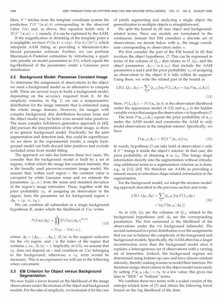
As suggested in [2], [32], an initial oversegmentation of theimage can efficiently recover most object boundaries.Adopting this approach, in our work, we use themorphological watershed algorithm [4]. Specifically, weuse the Brightness-Gradient boundary strength function in[29] to obtain both edges and markers; we extract the latterfrom the local minima of the boundary strength function.As shown in Fig. 5, this gives us a small set of imagefragments that we use in two complementary ways.

First, we define a background distribution by modelingthe image intensities within each fragment with a normaldistribution. We thereby build our piecewise-constantbackground model with a set of fixed regions.

Second, since these regions are highly cohesive, we treatthem as “bundled” observations—or “atomic regions” in [2]and “superpixels” in [32]. We thus use a fragment-basedE-step that uniformly assigns an image fragment to eitherthe object or the background hypothesis. This reduces thenumber of assignment variables considered from thenumber of pixels to the number of fragments.

We now consider the part of the EM criterion involvingobservations in region Rr by limiting the summation in (17)to n 2 Rr. We can simplify its expression by noting first that

only the background submodel Br built within region r isactive and then using a common value Qr;k for the relatedassignment variables Qn;k, n 2 Rr. Further, since only theobject and a single background hypothesis are entailed, weset qr ¼ Qr;O ¼ 1�Qr;Br for simplicity. We can thus rewritethe considered part of (17) as

LBðI; qr;AÞ ¼Xn2Rr

qr logP ðInjAOÞ þ logP ðzn;OjAOÞ� �

þ ð1� qrÞ logP ðInjABrÞ þ logP ðzn;Br jABrÞ� �

� 1

�qr log qr þ ð1� qrÞ logð1� qrÞ½ �:

Substituting from (15) and maximizing with respect to qrgives

1

�log

qr1� qr

� � ¼ 1

jRrjXn2Rr

logP ðInjAOÞH S�1ðxn; sÞð Þ

P ðInjABrÞ;

ð18Þ

where � ¼ log �O�Br

and jRrj is the cardinality of region r. We

treat � as a design parameter that allows us to determine

how easily we assign fragments to the object. Finally, we

use the notation log P ðIjOÞP ðIjBÞ for the right-hand side of (18), so

the optimal qr is given by a sigmoidal function:

qr ¼1

1þ exp �� log P ðIjOÞP ðIjBÞ þ �

h i� � : ð19Þ

For all experiments, we use the values � ¼ 10 and � ¼ 1,estimated by tuning the system’s performance on a fewimages. We note that a different front-end segmentationalgorithm might require different values for � and �. Forexample, if the segments returned were significantlysmaller, a lower value for � would be needed: As arguedin Section 3.3, in that case, the background model wouldgenerally be more accurate, so we would need to make it


Fig. 5. Fragment-based E-step. We break the image into fragmentsusing the watershed algorithm, as shown in (a). The background modeluses a Gaussian distribution within each fragment and its prediction,shown in (b), is constant within each fragment. During the E-step, theoccupation of fragments is determined based on whether the objectsynthesis Iðx; s; tÞ reconstructs the image better than the backgroundmodel. The gray value indicates the degree to which a fragment isassigned to the object. (a) Watershed segmentation. (b) Backgroundsynthesis. (c) Fragment-based E-step.

even easier for the foreground model to acquire a part. Toavoid manual tuning, one can therefore use the simple

learning-based approach we had initially used in [21] to

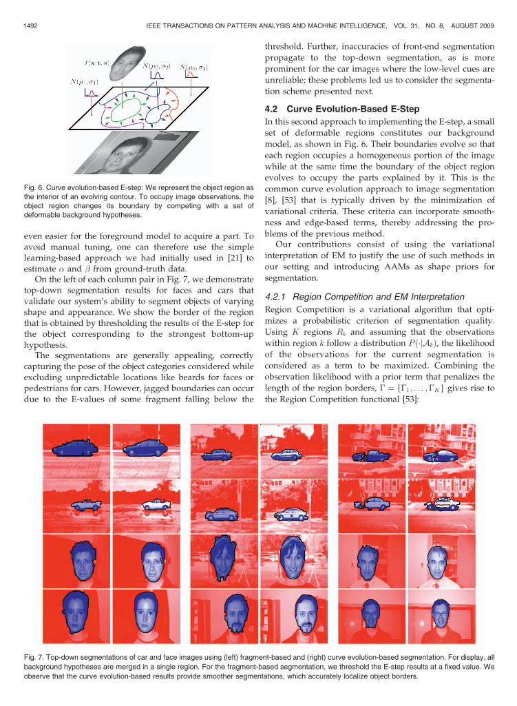
estimate � and � from ground-truth data.On the left of each column pair in Fig. 7, we demonstrate

top-down segmentation results for faces and cars that

validate our system’s ability to segment objects of varying

shape and appearance. We show the border of the regionthat is obtained by thresholding the results of the E-step for

the object corresponding to the strongest bottom-uphypothesis.

The segmentations are generally appealing, correctly

capturing the pose of the object categories considered while

excluding unpredictable locations like beards for faces orpedestrians for cars. However, jagged boundaries can occur

due to the E-values of some fragment falling below the

threshold. Further, inaccuracies of front-end segmentation

propagate to the top-down segmentation, as is more

prominent for the car images where the low-level cues are

unreliable; these problems led us to consider the segmenta-

tion scheme presented next.

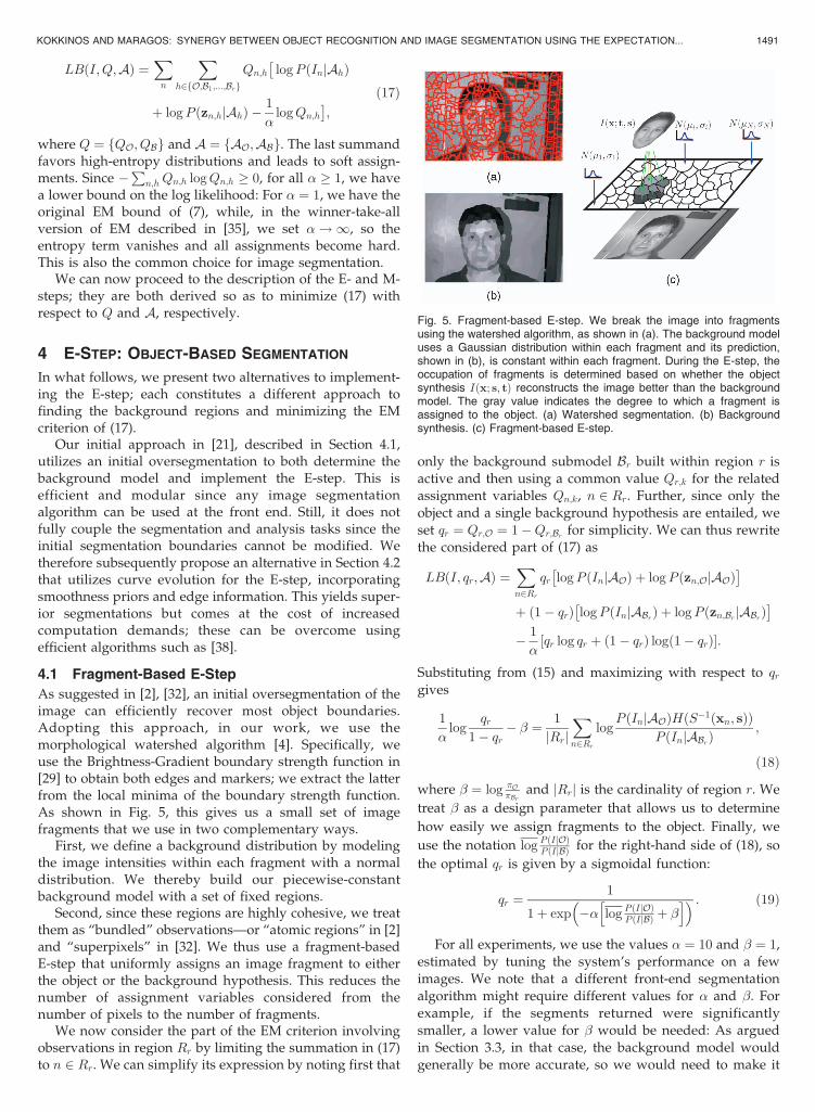
4.2 Curve Evolution-Based E-Step

In this second approach to implementing the E-step, a small

set of deformable regions constitutes our background

model, as shown in Fig. 6. Their boundaries evolve so that

each region occupies a homogeneous portion of the image

while at the same time the boundary of the object region

evolves to occupy the parts explained by it. This is the

common curve evolution approach to image segmentation

[8], [53] that is typically driven by the minimization of

variational criteria. These criteria can incorporate smooth-

ness and edge-based terms, thereby addressing the pro-

blems of the previous method.Our contributions consist of using the variational

interpretation of EM to justify the use of such methods in

our setting and introducing AAMs as shape priors for

segmentation.

4.2.1 Region Competition and EM Interpretation

Region Competition is a variational algorithm that opti-

mizes a probabilistic criterion of segmentation quality.

Using K regions Rk and assuming that the observations

within region k follow a distribution P ð�jAkÞ, the likelihood

of the observations for the current segmentation is

considered as a term to be maximized. Combining the

observation likelihood with a prior term that penalizes the

length of the region borders, � ¼ f�1; . . . ;�Kg gives rise to

the Region Competition functional [53]:


Fig. 6. Curve evolution-based E-step: We represent the object region as

the interior of an evolving contour. To occupy image observations, the

object region changes its boundary by competing with a set of

deformable background hypotheses.

Fig. 7. Top-down segmentations of car and face images using (left) fragment-based and (right) curve evolution-based segmentation. For display, all

background hypotheses are merged in a single region. For the fragment-based segmentation, we threshold the E-step results at a fixed value. We

observe that the curve evolution-based results provide smoother segmentations, which accurately localize object borders.

Jð�;AÞ ¼XKk¼1

�

2

Z�k

ds�Z Z

Rk

logP IðxÞjAkð Þdx; ð20Þ

where � controls the prior’s weight. The calculus ofvariations yields the evolution law for the kth border:

@�k@t¼ ��N þ log

P IðxÞjAkð ÞP IðxÞjAmð ÞN ; ð21Þ

where P ðIðxÞjAmÞ is the log likelihood of IðxÞ under thecompeting neighboring hypothesis m, � is the kth bordercurvature, and N is its outward normal unit vector. Aregion boundary moving according to (21) assigns observa-tions to the region that predicts them better whilemaintaining the borders smooth, as it minimizes thefunctional (20).

There is an intuitive link between Region Competitionand EM: The E-step is similar to curve evolution, whereobservations are assigned to region hypotheses, and theM-step is similar to updating the parameters of the regiondistributions. The difference is that instead of a generic EMclustering scheme that treats an image as an unordered setof pixels, Region Competition brings in useful geometricinformation and considers only hard assignments ofobservations to hypotheses.

The formal link we build relies on using the varia-tional interpretation of EM to restrict the distributionsconsidered during the minimization of (17) with respectto Qn;k. Specifically, we consider only binary winner-take-all [35] distributions over assignments. Denoting the setof observations that are assigned to hypothesis k asRk ¼ fn : Qn;k ¼ 1g, the first term of (17) writesX

n

Xk

Qn;k logP ðInjAkÞ ¼Xk

Xn2Rk

logP ðInjAkÞ; ð22Þ

which is a discretization of the area integral in (20).Further, we can introduce the arc-length penalty of (20)

into our EM criterion by appropriately constructing theprior on the hidden variables, i.e., the second term in (8).For this, we introduce a Boolean function bðzN n

Þ whoseargument is the window of assignment vectors in theneighborhood N n of n. b indicates whether observationsaround n are assigned to different hypotheses, i.e., if n is ona boundary; we use b to write the length-based prior:

P ðZÞ ¼ 1

Z

Yn

exp �bðzN nÞ

� �; ð23Þ

where Z is a normalizing constant. We could also considerobject specific terms, but we assume P ðZjAÞ ¼ P ðZÞ forsimplicity. Since Q is factorizable and

Pk Qn;k ¼ 1, we have

�X

Z

QðZÞ logP ðZjAÞ ¼Xn

Xk

Qn;kbðzN nÞ þ c

¼Xn

bðzN nÞ þ c;

which is, apart from the constant c ¼ logZ, a discretizedversion of the arc-length penalty used in Region Competition.

Finally, the entropy term �P

Z QðZÞ logQðZÞ of (17)generally favors smooth assignments of observations to theavailable hypotheses; since the Region Competition scheme

by design assigns in a hard manner image observations to

regions, this term always equals zero and does not affect the

EM bound. We note that we would end up with the same

result if we set � ¼ 1 in (17) from the start; then, the

entropy term would vanish and the optimal distributions

would be binary.Summing up, we can see Region Competition as

minimizing a version of (17) that utilizes specific expres-

sions for P ðZjAÞ and QðZÞ. Even though mostly technical,

this link allows us to use well-studied segmentation

algorithms in our system without straying from the original

EM-based formulation.

4.2.2 AAMs as Shape Priors

Coming to our case, the data fidelity terms for both the

object and background hypotheses break into sums over the

image grid, so they directly fit the setting of Region

Competition. A variation stems from the P ðzn;OjAOÞ and

P ðzn;BjABÞ terms that enforce prior information on the

assignment probabilities. As mentioned in the previous

section, P ðzn;OjAOÞ prevents the object from obtaining

observations that do not fall within the template support;

P ðzn;OjABÞ can be a small constant that acts as a penalty on

the background model and helps the foreground model

obtain observations more easily.By taking into account the P ðzn;OjAOÞ and P ðzn;BjABÞ

terms, we have the following evolution law for the front �

that separates the object O and the background Bhypotheses:

@�

@t¼ � ��N þ log

P IðxÞjAOð ÞP znðxÞ;OjAO� �

P IðxÞjABð ÞP znðxÞ;BjAB� � N

¼ð15Þ ��þ logP IðxÞjAOð ÞH S�1ðx; sÞð Þ

P IðxÞjABð Þ þ ��

N :

Above � ¼ log �O�Br

, x is an image location through which the

front passes and nðxÞ is the corresponding observation

index. The term HðS�1ðx; sÞÞ gates the motion due to the

observation likelihood ratio term, log P ðIðxÞjAOÞP ðIðxÞjABÞ . Specifically,

it lets the object compete only for observations that fall

within its support, i.e., if HðS�1ðx; sÞÞ ¼ 1. Otherwise, the

observation is assigned to the background.This constrains the object region to respect the shape

properties of the corresponding category and introduces

shape knowledge in the segmentation. Contrary to other

works such as [11], [43], this does not require additional

shape prior terms but comes naturally from the AAM

modeling assumptions.Further, as in the previous section, we use a positive

balloon force �, which favors the object region over the

background.We also use terms that result in improved segmentations,

even if they do not stem from a probabilistic treatment.

Specifically, as in [39], an edge-based term is utilized that

pushes the segment borders toward strong intensity

variations:


@�

@t¼�� þ log

P IðxÞjs; tð ÞH S�1ðx; sÞð ÞP IðxÞjABð Þ

þ � �rG jrIjð Þ � NN ;

ð24Þ

whereGðjrIjÞ is a decreasing function of edge strength jrIj.Curve evolution is implemented using level-set methods

[37], [44], which are particularly well suited for our

problem; their topological flexibility allows holes to appear

in the interior of regions, thereby excluding occluded object

areas. Two competing background fronts are introduced

which form two large clusters for bright and dark regions.

Initialization is random for all but the object fronts that are

centered around the bottom-up detection results. Finally,

we smooth H with a Gaussian kernel of � ¼ 2 for stability.In Fig. 7, where we compare the top-down segmentations

offered by the two approaches, we observe that curve

evolution yields superior results. The curvature term results

in smooth boundaries, the edge force accurately localizes

object borders, the shape of the objects is correctly captured,

and occluded areas are discarded. Some partial failures,

e.g., the bottom-left car image, can be attributed to the

limited expressive ability of the AAM, which could not

capture the specific illumination pattern. In that respect, the

modularity offered by the EM algorithm is an advantage,

since any better generative model can be incorporated in the

system once available.

5 M-STEP—PARAMETER ESTIMATION

In the M-step, the model parameters are updated to account

for the observations assigned to the object during the E-step.

The generative models we use assume a Gaussian noise

process so that parameter estimation amounts to weighted

least squares minimization, where the weights are provided

by the E-step: Higher weights are given to observations

assigned with high confidence to the object and vice versa.This approach faces occlusions by discounting them

during model fitting. The typical AAM approach, e.g., [40],

either considers that occluded areas are known or utilizes a

robust norm to reduce their effect on fitting. Instead,

viewing AAMs in the generative model/EM setting tackles

this problem by allowing alternative hypotheses to explain

the observations, without modifying the AAM error norm.

5.1 EM-Based AAM Fitting Criterion

In order to derive the update equations for the object

parameters AO ¼ ðs; tÞ, we ignore the entropy-related term

of the EM criterion (17) since it does not affect the final

update. Further, the support-related term HðS�1ðx; sÞÞ of

(11) is hard to deal with inside the logarithm: It can equal

zero and introduce infinite values in the optimized

criterion. To avoid this, we notice that any observation

falling outside the support cannot be assigned to the object,

by default. Therefore, we multiply the object weights

delivered by the E-step with the indicator function, which

has the desired effect of taking the object support into

account. The quantity maximized is thus

CEMðs; tÞ ¼X

x

EðxÞH S�1ðx; sÞ� �

logP IðxÞjAOð Þ

þ 1� EðxÞH S�1ðx; sÞ� ��

logP IðxÞjABð Þ;ð25Þ

where EðxÞ ¼ QnðxÞ;O are the results of the previous E-step,

obtained according to one of the two schemes in the previous

section. Introducing the constant c ¼P

x logP ðIðxÞjABÞ and

gathering terms, we rewrite (25) as

CEMðs; tÞ ¼X

x

EðxÞH S�1ðx; sÞ� �

logP IðxÞjAOð ÞP IðxÞjABð Þ þ c: ð26Þ

Ignoring c, which is unaffected by the optimization of theforeground model and working on the template coordinatesystem, this criterion writes

CEMðs; tÞ ¼X

x

EðxsÞHðxÞDðx; sÞ logP IðxsÞjAOð ÞP IðxsÞjABð Þ ; ð27Þ

where we introduce the notation xs ¼ Sðx; sÞ. Since thedeformation x! SðxÞ locally rescales the template domain,the determinant of its Jacobian, Dðx; sÞ, commeasures (26)and (27), which are viewed as discretizations of areaintegrals. Finally, modeling both the foreground and back-ground reconstruction errors as a white Gaussian noiseprocess, we write (27) as

CEMðs; tÞ ¼X

x

EðxsÞHðxÞDðx; sÞ

� IðxsÞ � T ðx; tÞð Þ2� IðxsÞ �BðxsÞð Þ2h i

;

ð28Þ

where T is the object-based synthesis and B is the imagereconstruction using the background model. The multi-plicative factor from the standard deviation of the noiseprocess is omitted since it does not affect the finalparameter estimate.

The standard least squares AAM criterion of (11) can betranscribed using this notation as

CLSðs; tÞ ¼X

x

HðxÞ IðxsÞ � T ðx; tÞð Þ2: ð29Þ

Comparing (28) and (29), we observe three main deficien-

cies of the latter: First, the segmentation information of

EðxsÞ is discarded, forcing the model to explain potentially

occluded areas. Second, the fidelity of the foreground and

background models to the data are not compared; in the

absence of strong edges, this leads to mismatches of the

image and model boundaries. Third, the magnification or

shrinking of template points due to the deformation is

ignored, while it is formally required by the generative

model approach.

5.2 Shape Fitting Equations

In the following, we provide update rules for AAM fittinggoing from (29) to (28), by gradually introducing moreelaborate terms. As in [30], we derive the optimal updatebased on a quadratic approximation to the cost; we providedetails in the Appendix, which can be found in theComputer Society Digital Library at http://doi.ieeecomputersociety.org/TPAMI.2008.158.


Perturbing the shape parameters by �s, we have

I Sðx; sþ�sÞð Þ ’ I Sðx; sÞð Þ þXNSi¼1

dI

dsiðx; sÞ�si; ð30Þ

dI

dsiðx; sÞ ¼ @I Sðx; sÞð Þ

@x

@Sx@siþ @I Sðx; sÞð Þ

@y

@Sy@si

; ð31Þ

whereNS is the number of shape basis elements. To write (30)concisely, we consider raster scanning the image whereby Ibecomes an N � 1 vector, where N is the number ofobservations, dI

ds becomes an N �NS matrix, while �s istreated as an NS � 1 vector. We can thus write (30) as

Iðsþ�sÞ ¼ IðsÞ þ dI

ds�s; ð32Þ

where IðsÞ denotes the vector formed by raster scanningIðSðx; sÞÞ; this is a notation we use in the following for allquantities appearing inside the criteria being optimized. Forsimplicity, we also omit the s argument from IðsÞ.

To write the quadratic approximation to the perturbedcost CLSðsþ�s; tÞ, we introduce E ¼ I�T and denote by the Hadamard product, ðaijÞ ðbijÞ ¼ ðaijbijÞ. We therebywrite

CLSðsþ�s; tÞ ¼ CLSðs; tÞ þ J�sþ 1

2�sTH�s;

J ¼ 2½H E�T dI

ds; H ¼ 2 H dI

s

�TdI

ds;

ð33Þ

where J is the Jacobian of the cost function and H is itsHessian. For terms like H dI

ds , where H is N � 1 and dIds is

N �NS , H is replicated NS times horizontally. From (33),we get the update of the forward additive method [30]:�s� ¼ �½JH�1�T .

Further, introducing the E-step results yields the follow-ing criterion:X

x

EðxsÞHðxÞ IðxsÞ � T ðx; tÞð Þ2¼ ½E H E�TE; ð34Þ

for which the Jacobian and Hessian matrices become

J ¼ 2ðH0 EÞT dI

dsþ ET dE

dsH E

�; ð35Þ

H ¼ 2 H0 dI

dsþ 2

dE

dsH E

� TdI

ds; ð36Þ

where H0 ¼ E H. Multiplication with E forces the fittingscheme to lock onto the areas assigned to the object andresults in the new termsET ðdE

ds H EÞand 2ðdEds H EÞT ðdI

dsÞ.These account for the change caused by �s in theprobability of assigning observations to template points.

A more elaborate expression results from incorporatingthe deformation’s Jacobian in the update; as it does notcritically affect performance, we only report it in theAppendix, which can be found in the Computer SocietyDigital Library at http://doi.ieeecomputersociety.org/TPAMI.2008.158.

Finally, we consider the reconstruction error of thebackground model, EB ¼ I�B, where B is the matrix

formed by raster scanning the background synthesis BðxsÞ.We thus obtain the cost function and Jacobian and Hessianmatrices for the original EM criterion (28):

CEMðs; tÞ ¼ ðH EÞ E½ �T ½E� � ðH EÞ EB½ �T ½EB�; ð37Þ

J ¼ J E � J EB ;H ¼ HE �HEB ; ð38Þ

where J E and HE are as in (35) and (36) and J EB and HEBare their background model counterparts. Since the mini-mized term is no longer convex, instabilities may occur. Anoptimal scaling of the update vector is therefore chosenwith bisection search, starting from one.

5.3 Appearance Fitting Equations

The appearance parameters are estimated by consideringthe part of the EM criterion that depends on the modelprediction:

CEMðs; tÞ ¼X

x

WðxÞ IðxsÞ � T 0ðxÞ �XNTi¼1

tiT iðxÞ" #2

; ð39Þ

where NT is the number of appearance basiselements, and W ðxÞ combines all scaling factors:WðxÞ ¼ Dðx; sÞHðxÞEðSðx; sÞÞ: This yields the weightedleast squares error solution:

t� ¼ W ðI�T0Þ½ �TTh i

; TT ðW TÞ� ��1

; ð40Þ

where T is the N �NT array formed by the appearancebasis elements.

Finally, a prior distribution learned during modelconstruction is introduced in the updates of both the sand t parameters. For an independent Gaussian distribu-tion, the Jacobian and Hessian matrices are modified as

J 0i ¼ J i þ pi�2i

; H0i;i ¼ Hi;i þ 1

�2i

; ð41Þ

where i ranges over the number of parameter vectorelements, pi is the ith element of the parameter estimateat the previous iteration, �i is its standard deviation on thetraining set, and controls the trade-off between priorknowledge and data fidelity.

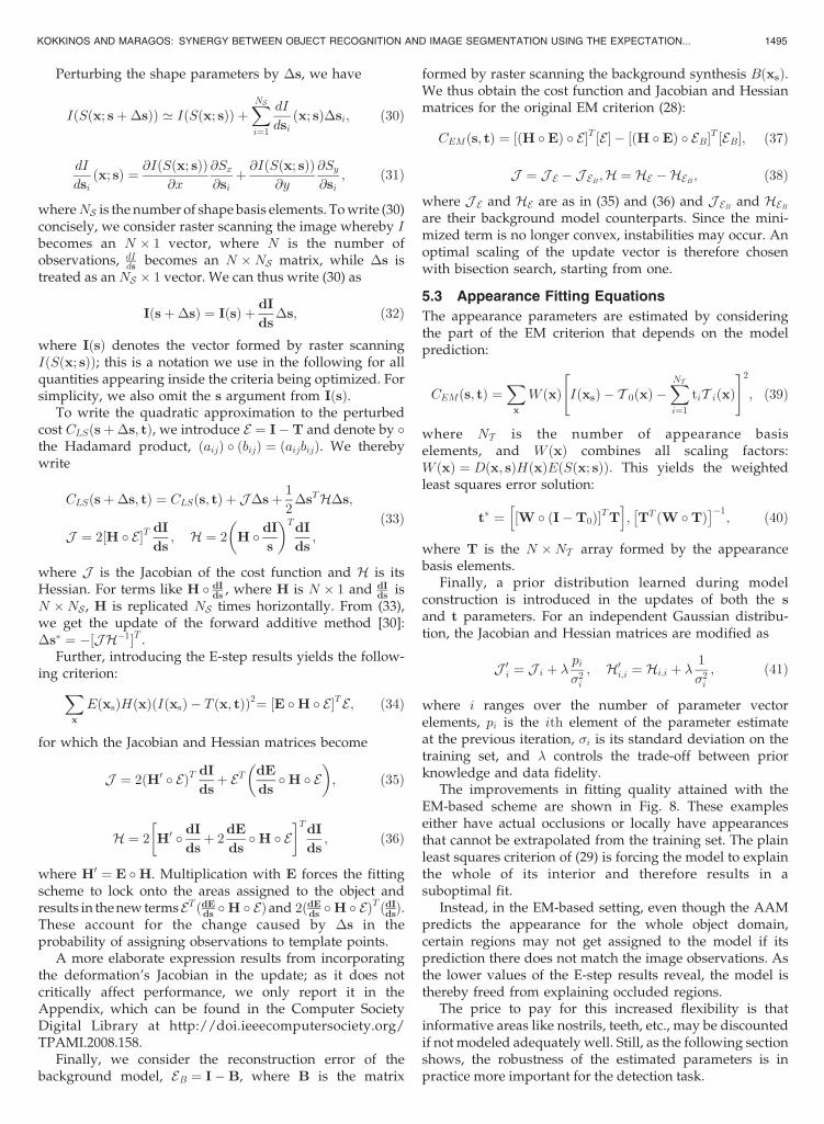
The improvements in fitting quality attained with theEM-based scheme are shown in Fig. 8. These exampleseither have actual occlusions or locally have appearancesthat cannot be extrapolated from the training set. The plainleast squares criterion of (29) is forcing the model to explainthe whole of its interior and therefore results in asuboptimal fit.

Instead, in the EM-based setting, even though the AAMpredicts the appearance for the whole object domain,certain regions may not get assigned to the model if itsprediction there does not match the image observations. Asthe lower values of the E-step results reveal, the model isthereby freed from explaining occluded regions.

The price to pay for this increased flexibility is thatinformative areas like nostrils, teeth, etc., may be discountedif not modeled adequately well. Still, as the following sectionshows, the robustness of the estimated parameters is inpractice more important for the detection task.


6 SYNERGETIC OBJECT CATEGORY DETECTION

Our goal in this section is to explore how the synergy

between segmentation and recognition improves detection

performance. This is a less explored side of the bottom-up/

top-down idea compared to top-down segmentation and, as

we show with the object categories of faces and cars, it is

equally practical and useful.

6.1 Detection Strategy

6.1.1 Bottom-Up Detection

We use a front-end object detection system to provide us

with all object hypotheses by setting its rejection threshold

to a conservative value. As in [45], we treat these detections

as proposals that are pruned via the bottom-up/top-down

loop. We rely on the point-of-interest-based system in [22],

which represents objects in terms of a codebook of primal

sketch features. This system builds object models by

clustering blobs, ridges, and edges extracted from the

training set and then forming a codebook representation.

During detection, the extracted features propose object

locations based on their correspondences with the codebook

entries. Since any other bottom-up system could be used

instead of this one, we refer to [22] for further details, as

well as to related literature on this quickly developing field,

e.g., [1], [7], [14], [25], [50].

6.1.2 Top-Down and Bottom-Up Combination

For object detection, we complement the bottom-up detec-

tion results with information obtained by the parameters of

the fitted AAM models and the segmentation obtained

during the E-step, as illustrated in Fig. 4. We thus have

three different cues for detection. First, the bottom-up

detection term CBU quantifies the likelihood of interest

point features given the hypothesized object location [22].Second, the AAM parameters are used to indicate how

close the observed image is to the object category. We

model the AAM parameter distributions as Gaussian

density functions, estimated separately on foreground and

background locations during training. We thereby obtain a

simple classifier:

CAAM ¼ logP ðs; tjOÞP ðs; tjBÞ ; ð42Þ

which decides about the presence of the object based on the

estimated AAM parameters.Third, we quantify how well the object hypothesis

predicts the image data using the E-step results that give

the probability EðxÞ of assigning observation x to the object.

We build the segmentation-based classifier by computing

the average of EðxÞ over the area that can be occupied by

the object:

CSEG ¼P

x H S�1ðxÞð ÞEðxÞPx H S�1ðxÞð Þ : ð43Þ

The summation is over the whole image domain and

HðS�1ðxÞÞ indicates whether x can belong to the object.

Using the E-step results in this way prunes false positives,

around which the AAM cannot explain a large part of the

image, thereby resulting in a low value of CSEG.We combine the three classifiers using the supra-

Bayesian fusion setting [19]. The output Ck of classifier k

is treated as a random variable, following the distributions

P ðCkjOÞ, P ðCkjBÞ under the object and background

hypotheses, respectively. Considering the set of classifier

outputs as a vector of independent random variables,

C ¼ ðC1; . . . ; CkÞ, we use their individual distributions for

classifier combination:

P ðOjCÞP ðBjCÞ ¼ c

P ðCjOÞP ðCjBÞ ¼ c

YKk¼1

P ðCkjOÞP ðCkjBÞ

; ð44Þ

where c ¼ P ðOÞ=P ðBÞ.


Fig. 8. Differences in AAM fitting using the EM algorithm. (a) Input image. (b) Plain least squares (LS) fit. (c) EM-based fit. (d) E-step results. The EM-

based fit outperforms the typical LS fit as the E-step results robustify the AAM parameter estimation. This is accomplished by discounting occlusions

or areas with unprecedented appearance variations, such as the third window and the hair fringe in the bottom row.

6.2 Experimental Results

6.2.1 Performance Evaluation and Experimental

Settings

We use Receiver Operating Characteristic (ROC) andPrecision Recall (PR) curves to evaluate a detector: ROCcurves consider deciding whether an image contains anobject, irrespective of its location. PR curves evaluate objectlocalization, comparing the ratio R of retrieved objects(recall) to the ratio P of correct detections (precision); bothcurves can be summarized using their Equal Error Rate(EER), namely, the point where the probability of a false hitequals the probability of a missed positive.

In order to compare our results with prior work, we haveused the setup in [14] for faces and that in [1] for cars. Carsare rescaled by a factor of 2.5 and flipped to have the samedirection during training, while faces are normalized so thatthe eye distance is 50 pixels; a 50 � 30 box is used to label adetected face a true hit. Further, nonmaximum suppressionis applied on the car results as in [1], allowing only thestrongest hypothesis to be active in a 100 � 200 box.

Regarding system tuning, we determine the parametersthat influence segmentation and model fitting using a fewimages from the training set of each category; duringtesting, we use the same parameter choices for bothcategories on all of the subsequent detection tasks.

6.2.2 Comparison of Alternative E-Step

Implementations

We initially compare the Fragment-based E-step (FE) andCurve-Evolution-based E-step (CE) approaches in terms oftheir appropriateness for object detection. Specifically, we

have applied the EM approach to both object categoriesconsidered, using identical settings for the detection frontend, the EM system components, and the classifiercombination.

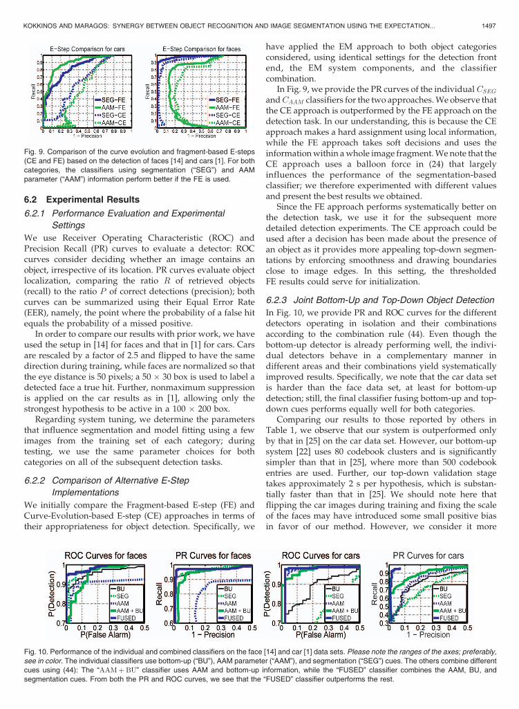
In Fig. 9, we provide the PR curves of the individual CSEGandCAAM classifiers for the two approaches. We observe thatthe CE approach is outperformed by the FE approach on thedetection task. In our understanding, this is because the CEapproach makes a hard assignment using local information,while the FE approach takes soft decisions and uses theinformation within a whole image fragment. We note that theCE approach uses a balloon force in (24) that largelyinfluences the performance of the segmentation-basedclassifier; we therefore experimented with different valuesand present the best results we obtained.

Since the FE approach performs systematically better onthe detection task, we use it for the subsequent moredetailed detection experiments. The CE approach could beused after a decision has been made about the presence ofan object as it provides more appealing top-down segmen-tations by enforcing smoothness and drawing boundariesclose to image edges. In this setting, the thresholdedFE results could serve for initialization.

6.2.3 Joint Bottom-Up and Top-Down Object Detection

In Fig. 10, we provide PR and ROC curves for the differentdetectors operating in isolation and their combinationsaccording to the combination rule (44). Even though thebottom-up detector is already performing well, the indivi-dual detectors behave in a complementary manner indifferent areas and their combinations yield systematicallyimproved results. Specifically, we note that the car data setis harder than the face data set, at least for bottom-updetection; still, the final classifier fusing bottom-up and top-down cues performs equally well for both categories.

Comparing our results to those reported by others inTable 1, we observe that our system is outperformed onlyby that in [25] on the car data set. However, our bottom-upsystem [22] uses 80 codebook clusters and is significantlysimpler than that in [25], where more than 500 codebookentries are used. Further, our top-down validation stagetakes approximately 2 s per hypothesis, which is substan-tially faster than that in [25]. We should note here thatflipping the car images during training and fixing the scaleof the faces may have introduced some small positive biasin favor of our method. However, we consider it more


Fig. 9. Comparison of the curve evolution and fragment-based E-steps

(CE and FE) based on the detection of faces [14] and cars [1]. For both

categories, the classifiers using segmentation (“SEG”) and AAM

parameter (“AAM”) information perform better if the FE is used.

Fig. 10. Performance of the individual and combined classifiers on the face [14] and car [1] data sets. Please note the ranges of the axes; preferably,

see in color. The individual classifiers use bottom-up (“BU”), AAM parameter (“AAM”), and segmentation (“SEG”) cues. The others combine different

cues using (44): The “AAMþ BU” classifier uses AAM and bottom-up information, while the “FUSED” classifier combines the AAM, BU, and

segmentation cues. From both the PR and ROC curves, we see that the “FUSED” classifier outperforms the rest.

important that systematic improvement in performance isobtained by combining top-down and bottom-up informa-

tion via the EM algorithm.After validating the usefulness of top-down information,

we address the question of whether the joint treatment of

the two tasks is really necessary. One particular concern hasbeen whether this improvement is exclusively due to the

AAM classifier; if this is so, this would render theEM approach superfluous for detection. The first answer

comes from comparing the results obtained by combiningall cues (“Fused”) with the ones using only the AAM and

bottom-up classifiers. For both cases considered, weobserve an improvement in both the ROC and PR curves,

which is due to the additional information provided by thesegmentation-based classifier. Still, what we consider more

important and now demonstrate is that EM allows for theuse of generative models in hard images by discounting

image variation that was not observed in the training set.

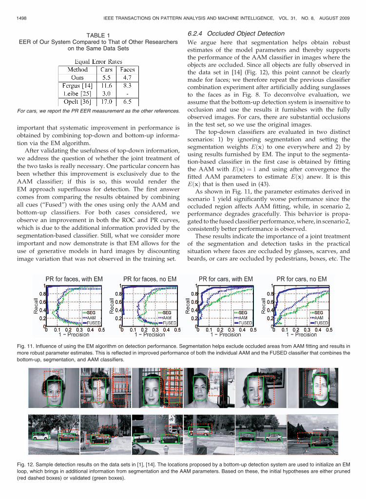
6.2.4 Occluded Object Detection

We argue here that segmentation helps obtain robustestimates of the model parameters and thereby supportsthe performance of the AAM classifier in images where theobjects are occluded. Since all objects are fully observed inthe data set in [14] (Fig. 12), this point cannot be clearlymade for faces; we therefore repeat the previous classifiercombination experiment after artificially adding sunglassesto the faces as in Fig. 8. To deconvolve evaluation, weassume that the bottom-up detection system is insensitive toocclusion and use the results it furnishes with the fullyobserved images. For cars, there are substantial occlusionsin the test set, so we use the original images.

The top-down classifiers are evaluated in two distinctscenarios: 1) by ignoring segmentation and setting thesegmentation weights EðxÞ to one everywhere and 2) byusing results furnished by EM. The input to the segmenta-tion-based classifier in the first case is obtained by fittingthe AAM with EðxÞ ¼ 1 and using after convergence thefitted AAM parameters to estimate EðxÞ anew. It is thisEðxÞ that is then used in (43).

As shown in Fig. 11, the parameter estimates derived inscenario 1 yield significantly worse performance since theoccluded region affects AAM fitting, while, in scenario 2,performance degrades gracefully. This behavior is propa-gated to the fused classifier performance, where, in scenario 2,consistently better performance is observed.

These results indicate the importance of a joint treatmentof the segmentation and detection tasks in the practicalsituation where faces are occluded by glasses, scarves, andbeards, or cars are occluded by pedestrians, boxes, etc. The


TABLE 1EER of Our System Compared to That of Other Researchers

on the Same Data Sets

For cars, we report the PR EER measurement as the other references.

Fig. 11. Influence of using the EM algorithm on detection performance. Segmentation helps exclude occluded areas from AAM fitting and results in

more robust parameter estimates. This is reflected in improved performance of both the individual AAM and the FUSED classifier that combines the

bottom-up, segmentation, and AAM classifiers.

Fig. 12. Sample detection results on the data sets in [1], [14]. The locations proposed by a bottom-up detection system are used to initialize an EM

loop, which brings in additional information from segmentation and the AAM parameters. Based on these, the initial hypotheses are either pruned

(red dashed boxes) or validated (green boxes).

gain is not only due to the validation information offered bya top-down segmentation but also due to the robust modelfitting that sustains the performance of the classifier thatuses the AAM parameters.

7 SURVEY AND DISCUSSION

Herein, we briefly discuss and compare related work onthis relatively new problem, to place our contributions in abroader context.

7.1 Previous Work on Joint Detection andSegmentation

We can classify most of the existing works on jointsegmentation and detection based on whether they useglobal or part-based object representations. Global ap-proaches [21], [45], [51] assume that a monolithic objectmodel can account for the shape and appearance variationof the object category and thereby take hold of all the imageobservations. Part-based models such as [7], [24], [25], [27],[52] offer a modular representation that is used to build thetop-down segmentation in a hybrid fashion, using high-level information wherever available and low-level cues tobring the rest of the object together [24], [52].

At a more detailed level, the approach in [45], [54]performs a stochastic search in the space of regions andhypotheses by extending the Data-Driven MCMC schemein [46] to include global generative models for objectcategories. During a search, object and generic regionhypotheses are generated, merged, split, or discarded,while their borders are localized by curve evolution usingRegion Competition [53]. Even though this approach iselegant, in a practical object detection application, onetypically only needs the probability of an object beingpresent, which, as we show here, can be efficiently andreliably estimated using the observation window containingthe object and EM instead of stochastic search.

Following a nongenerative approach, codebook repre-sentations are used for joint detection and segmentation in[6], [7], and [25]. Figure-ground maps associated with thecodebook entries are stored during training and usedduring detection to assemble a segmentation of the object.Even though good performance is demonstrated in [6], [25],the segmentation depends on the ability to cover a largearea of the object using overlapping patches, necessitatingcomplex models. In another approach using a part-basedrepresentation in [52], an object-sensitive affinity measure isintroduced and pairwise clustering methods are used tofind a global minimum of the data partitioning cost. Theaffinity measure used leads to a grouping of pixels based onboth low-level cues (absence of edges and similarity) andhigh-level knowledge. However, the lack of a probabilisticinterpretation impedes the cooperation with other pro-cesses, while the detection task is not considered.

Coming to work involving the EM algorithm, we note firstthat the use of the EM algorithm for image segmentationproblems is certainly not novel; it has been used previouslyfor low-level problems such as feature-based image segmen-tation [3] or layered motion estimation [49]. Further, in [24], apart-based object representation is combined with the graph-cut algorithm to derive a top-down segmentation, yielding

accurate results for articulated object segmentation. TheEM algorithm is used there as well but in an optimizationrather than a generative model fitting task: The shapeparameters are treated as hidden variables and the E-stepconstructs a nonparametric shape distribution. The M-stepthen amounts to the maximization via graph cuts of asegmentation quality cost that entails the distributionconstructed in the E-step. This deviates from the use ofEM in the generative model setting, where parameterestimation is accomplished in the M-step. As we showhere, the generative model approach allows the principledcombination of different methodologies, like curve evolu-tion and AAMs, while minimizing the choices that ageneric optimization approach requires.

Further, in [16], [51], the EM algorithm is used toperform an object-specific segmentation of an image usingthe “sprites & layers” model, where the E-step assignsobservations to objects (“sprites”), and the M-step updatesthe object parameters. Intuitively, this approach is similar toours, but the interaction of the two processes is notexplored: The background model is estimated from a fixedset of images, thereby introducing strong prior knowledgethat is not available for the general segmentation problem,while it is not actually determined whether an object ispresent in the image, based on either bottom-up or top-down cues. Further, the deformations used do not modelthe object category shape variation since they either arerestricted to affine transformations [16] or use an MRF prioron a piecewise constant deformation field [51].

7.2 Previous Work on Shape Prior Segmentation

Complementary to research on top-down/bottom-up inte-gration, progress has been made during the last years in theuse of object-specific shape prior knowledge for imagesegmentation, e.g., in [10], [11], [26], [42], [43]. By focusingon the object boundaries, these approaches efficientlyexploit shape knowledge to overcome noise and partialocclusions.

Most shape prior methods rely on the implicit represen-tation of level-set methods, where a curve is represented interms of an embedding function such as the distancetransform. This allows for a convenient combination withcurve evolution methods: The variational criterion drivingthe segmentation is augmented with a shape-relatedpenalty term that is expressed in terms of the embeddingfunction of the evolving curve. This allows for thecombination of shape-based and image-based cues in acommon curve evolution framework.

Even though such methods do not model object aspectslike appearance or deformation statistics, they have beenproven particularly effective in tasks such as medical imagesegmentation [42] or tracking a detected person [10]. On theone hand, this can be seen as an advantage since lessdemanding object models are used; on the other hand, webelieve that they do not provide a complete solution to thebottom-up/top-down combination problem.

Specifically, part of the object may be occluded, so theboundaries of the object and the region assigned to it do nothave to be related. For example, if we consider a personwearing a hat or sunglasses, a shape prior-driven segmen-tation will force the curve corresponding to the object


hypothesis to include the occluded parts of the head, asmost heads are roughly ellipsoidal. Even though one canargue that this indicates robustness to occlusion, in ourunderstanding, a top-down segmentation should indicatethe image regions occupied by an object. This can beaccomplished with our approach, where a generative modellike an AAM can still fit the shape of the object, but, in theE-step, the occluded parts are not assigned to the object.

We should mention that the shape-prior-based technol-ogy has made advances in a broader range of problems likearticulated object tracking and tracking under severeocclusion using limited appearance information, e.g., [10],so this added functionality of our system can be seen asbeing complementary. However, the EM/generative modelapproach has no fundamental limitation in addressing theseproblems as well. Part-based deformation models can beused for articulated objects, while temporal coherence fortracking can be enforced by using a dynamical model forthe generative model parameters. Having proven the meritof the EM approach on a more constrained problem, wewould like to explore these more challenging directions infuture research.

8 CONCLUSIONS—FUTURE WORK

In this paper, we have addressed the problem of the jointsegmentation and analysis of objects, casting it in theframework of the EM algorithm. Apart from a conciseformulation of bottom-up/top-down interaction, this hasfacilitated the principled combination of different computervision techniques. Based on the EM algorithm, we havebuilt a system that can segment in a top-down mannerimages of objects belonging to highly variable categories,while also significantly improving detection performance.Summing up, the EM framework offers a probabilisticformulation for a recently opened problem and deals withits multifaceted nature in a principled manner.

An essential direction for rendering this approachapplicable to a broader set of problems is the automatedconstruction of models for generic objects; recent advances[7], [14], [50] have initiated a surge of activity on simplepart-based representations, e.g., [1], [22], [25], but little workhas been done for global generative models [23], [51].Further, a point that deserves deeper inspection is thecombination of low-level cues with part-based and globalgenerative models for joint object segmentation, which hasonly been partially tackled [22], [24], [52]. In future work,we intend to address these issues in the framework ofgenerative models with the broader goal of integratingdifferent computer vision problems in a unified andpractical approach.

ACKNOWLEDGMENTS

The authors thank G. Papandreou for the discussions onAAM fitting and for indicating related references. Theywish to thank the reviewers for their constructive commentsthat helped improve the quality of the paper. This work wassupported by the Greek Ministry of Education researchprogram “HRAKLEITOS” and by the European Network ofExcellence “MUSCLE.” Iasonas Kokkinos was with theNational Technical University of Athens when this paperwas first written.

REFERENCES

[1] S. Agarwal and D. Roth, “Learning a Sparse Representation forObject Detection,” Proc. Seventh European Conf. Computer Vision,2002.

[2] A. Barbu and S.C. Zhu, “Graph Partition by Swendsen-WangCuts,” Proc. Ninth Int’l Conf. Computer Vision, 2003.

[3] S. Belongie, C. Carson, H. Greenspan, and J. Malik, “Color- andTexture-Based Image Segmentation Using EM and Its Applicationto Content-Based Image Retrieval,” Proc. Sixth Int’l Conf. ComputerVision, 1998.

[4] S. Beucher and F. Meyer, “The Morphological Approach toSegmentation: The Watershed Transformation,” Math. Morphologyin Image Processing, E.R. Dougherty, ed., pp. 433-481, MarcelDekker, 1993.

[5] C. Bishop, “Latent Variable Models,” Learning in Graphical Models,M. Jordan, ed., MIT Press, 1998.

[6] E. Borenstein, E. Sharon, and S. Ullman, “Combining Top Downand Bottom-Up Segmentation,” Proc. IEEE Conf. Computer Visionand Pattern Recognition, 2004.

[7] E. Borenstein and S. Ullman, “Class-Specific, Top-Down Segmen-tation,” Proc. Seventh European Conf. Computer Vision, 2002.

[8] V. Caselles, R. Kimmel, and G. Sapiro, “Geodesic ActiveContours,” Int’l J. Computer Vision, vol. 22, no. 1, pp. 61-79, 1997.

[9] T. Cootes, G.J. Edwards, and C. Taylor, “Active AppearanceModels,” IEEE Trans. Pattern Analysis and Machine Intelligence,vol. 23, no. 6, pp. 681-685, June 2001.

[10] D. Cremers, “Dynamical Statistical Shape Priors for Level SetBased Tracking,” IEEE Trans. Pattern Analysis and MachineIntelligence, vol. 28, no. 8, pp. 1262-1273, Aug. 2006.

[11] D. Cremers, N. Sochen, and C. Schnorr, “Towards RecognitionBased Variational Segmentation Using Shape Priors and DynamicLabelling,” Proc. Fourth Int’l Conf. Scale Space, 2003.

[12] P. Dayan, G. Hinton, R. Neal, and R. Zemel, “The HelmholtzMachine,” Neural Computation, vol. 7, pp. 889-904, 1995.

[13] A. Dempster, N. Laird, and D. Rudin, “Maximum Likelihood fromIncomplete Data via the EM Algorithm,” J. Royal Statistical Soc.,Series B, 1977.

[14] R. Fergus, P. Perona, and A. Zisserman, “Weakly SupervisedScale-Invariant Learning of Models for Visual Recognition,” Int’l J.Computer Vision, vol. 71, no. 3, pp. 273-303, 2007.

[15] V. Ferrari, T. Tuytelaars, and L.V. Gool, “Simultaneous ObjectRecognition and Segmentation by Image Exploration,” Proc.Eighth European Conf. Computer Vision, 2004.

[16] B. Frey and N. Jojic, “Estimating Mixture Models of Images andInferring Spatial Transformations Using the EM Algorithm,” Proc.IEEE Conf. Computer Vision and Pattern Recognition, 1999.

[17] U. Grenander, General Pattern Theory. Oxford Univ. Press, 1993.[18] T. Jaakkola, “Tutorial on Variational Approximation Methods,”

Advanced Mean Field Methods: Theory and Practice. MIT Press, 2000.[19] R. Jacobs, “Methods for Combining Experts’ Probability Assess-

ments,” Neural Computation, no. 7, pp. 867-888, 1995.[20] M. Jones and T. Poggio, “Multidimensional Morphable Models: A

Framework for Representing and Matching Object Classes,” Int’l J.Computer Vision, vol. 29, no. 2, pp. 107-131, 1998.

[21] I. Kokkinos and P. Maragos, “An Expectation MaximizationApproach to the Synergy between Object Categorization andImage Segmentation,” Proc. 10th Int’l Conf. Computer Vision, 2005.

[22] I. Kokkinos, P. Maragos, and A. Yuille, “Bottom-Up and Top-Down Object Detection Using Primal Sketch Features andGraphical Models,” Proc. IEEE Conf. Computer Vision and PatternRecognition, 2006.

[23] I. Kokkinos and A. Yuille, “Unsupervised Learning of ObjectDeformation Models,” Proc. 11th Int’l Conf. Computer Vision, 2007.

[24] M.P. Kumar, P.H.S. Torr, and A. Zisserman, “Obj Cut,” Proc. IEEEConf. Computer Vision and Pattern Recognition, 2005.

[25] B. Leibe, A. Leonardis, and B. Schiele, “Combined ObjectCategorization and Segmentation with an Implicit Shape Model,”Proc. ECCV Workshop Statistical Learning in Computer Vision, 2004.

[26] M. Leventon, O. Faugeras, and E. Grimson, “Statistical ShapeInfluence in Geodesic Active Contours,” Proc. IEEE Conf. ComputerVision and Pattern Recognition, 2000.

[27] A. Levin and Y. Weiss, “Learning to Combine Bottom-Up andTop-Down Segmentation,” Proc. Ninth European Conf. ComputerVision, 2006.

[28] D. Marr, Vision. W.H. Freeman, 1982.


[29] D. Martin, C. Fowlkes, and J. Malik, “Learning to Detect NaturalImage Boundaries Using Local Brightness, Color, and TextureCues,” IEEE Trans. Pattern Analysis and Machine Intelligence,vol. 26, no. 5, pp. 530-549, May 2004.

[30] I. Matthews and S. Baker, “Active Appearance Models Revisited,”Int’l J. Computer Vision, vol. 60, no. 2, pp. 135-164, 2004.

[31] R. Milanese, H. Wechsler, S. Gil, J.M. Bost, and T. Pun,“Integration of Bottom-Up and Top-Down Cues for VisualAttention Using Non-Linear Relaxation,” Proc. IEEE Conf. Com-puter Vision and Pattern Recognition, 1994.

[32] G. Mori, X. Ren, A. Efros, and J. Malik, “Recovering Human BodyConfigurations: Combining Segmentation and Recognition,” Proc.IEEE Conf. Computer Vision and Pattern Recognition, 2004.

[33] D. Mumford, “Neuronal Architectures for Pattern TheoreticProblems,” Large Scale Theories of the Cortex. MIT Press, 1994.

[34] D. Mumford, “Pattern Theory: A Unifying Approach,” Perceptionas Bayesian Inference, 1996.

[35] R. Neal and G. Hinton, “A View of the EM Algorithm that JustifiesIncremental, Sparse and Other Variants,” Learning in GraphicalModels, M. Jordan, ed., 1998.

[36] A. Opelt, A. Fussenegger, and P. Auer, “Weak Hypotheses andBoosting for Generic Object Detection and Recognition,” Proc.Eighth European Conf. Computer Vision, 2004.

[37] S. Osher and J. Sethian, “Fronts Propagating with Curvature-Dependent Speed: Algorithms Based on Hamilton-Jacobi For-mulations,” J. Computational Physics, vol. 79, pp. 12-49, 1988.

[38] G. Papandreou and P. Maragos, “Multigrid Geometric ActiveContour Models,” IEEE Trans. Image Processing, vol. 16, no. 1,pp. 229-240, 2007.

[39] N. Paragios and R. Deriche, “Geodesic Active Regions: A NewParadigm to Deal with Frame Partition Problems in ComputerVision,” J. Visual Comm. and Image Representation, vol. 13, pp. 249-268, 2002.

[40] R. Gross, I. Matthews, and S. Baker, “Active Appearance Modelswith Occlusion,” Image and Vision Computing, vol. 24, no. 6,pp. 593-604, 2006.

[41] R. Rao and D. Ballard, “Dynamic Model of Visual RecognitionPredicts Neural Response Properties in the Visual Cortex,” VisionResearch, vol. 9, pp. 721-763, 1997.

[42] M. Rousson and D. Cremers, “Efficient Kernel Density Estimationof Shape and Intensity Priors for Level Set Segmentation,” Proc.Eighth Int’l Conf. Medical Image Computing and Computer AssistedIntervention, 2005.

[43] M. Rousson and N. Paragios, “Shape Priors for Level SetRepresentations,” Proc. Seventh European Conf. Computer Vision,2002.

[44] J. Sethian, Level Set Methods. Cambridge Univ. Press, 1996.[45] Z.W. Tu, X. Chen, A. Yuille, and S.C. Zhu, “Image Parsing:

Unifying Segmentation, Detection, and Recognition,” Int’l J.Computer Vision, vol. 63, no. 2, pp. 113-140, 2005.

[46] Z.W. Tu and S.C. Zhu, “Image Segmentation by Data-DrivenMCMC,” IEEE Trans. Pattern Analysis and Machine Intelligence,vol. 24, no. 5, pp. 657-673, May 2002.

[47] M. Turk and A. Pentland, “Eigenfaces for Recognition,”J. Cognitive Neuroscience, vol. 3, no. 1, pp. 71-86, 1991.

[48] S. Ullman, “Sequence Seeking and Counterstreams,” Large ScaleTheories of the Cortex. MIT Press, 1994.

[49] Y. Weiss and E. Adelson, “Perceptually Organized EM: AFramework for Motion Estimation That Combines Informationabout Form and Motion,” Proc. Fifth Int’l Conf. Computer Vision,1995.

[50] M. Welling, M. Weber, and P. Perona, “Unsupervised Learning ofModels for Recognition,” Proc. Sixth European Conf. ComputerVision, 2000.

[51] J. Winn and N. Jojic, “LOCUS: Learning Object Classes withUnsupervised Segmentation,” Proc. 10th Int’l Conf. ComputerVision, 2005.

[52] S. Xu and J. Shi, “Object Specific Figure-Ground Segregation,”Proc. IEEE Conf. Computer Vision and Pattern Recognition, 2003.

[53] S.C. Zhu and A. Yuille, “Region Competition: Unifying Snakes,Region Growing and Bayes/MDL for Multiband Image Segmen-tation,” IEEE Trans. Pattern Analysis and Machine Intelligence,vol. 18, no. 9, pp. 884-900, Sept. 1996.

[54] S.C. Zhu, R. Zhang, and Z.W. Tu, “Integrating Top-Down/Bottom-Up for Object Recognition by Data-Driven Markov ChainMonte Carlo,” Proc. IEEE Conf. Computer Vision and PatternRecognition, 2000.

Iasonas Kokkinos received the diploma inelectrical and computer engineering and thePhD degree from the National Technical Uni-versity of Athens, Greece, in 2001 and 2006,respectively. During 2004, he visited with theOdyssee team at Sophia-Antipolis, France, and,in 2006, he joined the Center for Image andVision Sciences at the University of California,Los Angeles, as a postdoctoral researcher. He iscurrently an assistant professor at the Ecole

Centrale Paris and an affiliate researcher at Equipe Galen, INRIA-Saclay. His research interests are in the broader fields of signalprocessing, computer vision, and pattern recognition, and in particular inthe application of statistical approaches to the solution of computervision tasks.. He has worked on texture segmentation, biologicallymotivated vision, and nonlinear dynamical modeling, while his currentresearch focus is on the combination of top-down approaches withbottom-up information for the problems related to object detection. Hehas served as a reviewer for the IEEE Transactions on Pattern Analysisand Machine Intelligence and IEEE Transactions on Image Processingand on the program committee of EMMCVPR ’07, ’09, CVPR ’09, andICCV ’07, ’09. He is a member of the IEEE.

Petros Maragos received the diploma in elec-trical engineering from the National TechnicalUniversity of Athens (NTUA) in 1980 and theMScEE and PhD degrees from the GeorgiaInstitute of Technology (Georgia Tech), Atlanta,in 1982 and 1985. In 1985, he joined the facultyof the Division of Applied Sciences, HarvardUniversity, Cambridge, Massachusetts, wherehe worked for eight years as a professor ofelectrical engineering. In 1993, he joined the

faculty of the School of Electrical and Computer Engineering (ECE) atGeorgia Tech. During parts of 1996-1998, he was on sabbatical andacademic leave, working as the director of research at the Institute forLanguage and Speech Processing, Athens. Since 1998, he has beenworking as a professor in the School of Electrical and ComputerEngineering, NTUA. His research and teaching interests include signalprocessing, systems theory, communications, pattern recognition, andtheir applications to image processing and computer vision, speechprocessing and recognition, and multimedia. He has served as anassociate editor for the IEEE Transactions on Acoustics, Speech, andSignal Processing and IEEE Transactions on Pattern Analysis andMachine Intelligence and as an editorial board member for the journalsSignal Processing and Visual Communications and Image Representa-tion. He has served as the general chairman or a cochair of severalconferences, including VCIP ’92, ISMM ’96, VLBV ’01, and MMSP ’07,and as a member of IEEE DSP committees. His research has receivedseveral awards, including a 1987 US National Science FoundationPresidential Young Investigator Award, the 1988 IEEE Signal Proces-sing (SP) Society’s Young Author Paper Award for the paper“Morphological Filters,” the 1994 IEEE SP Senior Award and the 1995IEEE Baker Award for the paper “Energy Separation in SignalModulations with Application to Speech Analysis,” the 1996 PatternRecognition Society’s Honorable Mention Award for the paper “Min-MaxClassifiers,” and the 2007 EURASIP Technical Achievements Award forcontributions to nonlinear signal processing and systems theory, imageprocessing, and speech processing. He was elected a fellow of the IEEEin 1995.

. For more information on this or any other computing topic,please visit our Digital Library at www.computer.org/publications/dlib.


Documents

Synergy between Object Recognition and Image Segmentation Using the Expectation-Maximization Algorithm