Synchrotron hard X-ray chemical imaging of trace element

JAAS

PAPER

Ope

n A

cces

s A

rtic

le. P

ublis

hed

on 3

0 Ja

nuar

y 20

20. D

ownl

oade

d on

3/1

2/20

22 6

:52:

41 A

M.

Thi

s ar

ticle

is li

cens

ed u

nder

a C

reat

ive

Com

mon

s A

ttrib

utio

n 3.

0 U

npor

ted

Lic

ence

.

View Article OnlineView Journal | View Issue

Synchrotron hard

aEawag, Swiss Federal Institute of Aquatic

133, 8600 Dubendorf, Switzerland. E-ma

[email protected]; Tel: +41 58 765 5336;bETH Zurich, Institute of Environmental EngcSwiss Light Source, Paul-Scherrer-InstitutedEMPA, Swiss Federal Laboratories for Ma

Gallen, SwitzerlandeETH Zurich, Institute of Energy Technology

† Electronic supplementary informa10.1039/c9ja00394k

Cite this: J. Anal. At. Spectrom., 2020,35, 567

Received 19th November 2019Accepted 27th January 2020

DOI: 10.1039/c9ja00394k

rsc.li/jaas

This journal is © The Royal Society o

X-ray chemical imaging of traceelement speciation in heterogeneous samples:development of criteria for uncertainty analysis†

Jonas Wielinski, *ab Francesco Femi Marafatto, ac Alexander Gogos, ad

Andreas Scheidegger, a Andreas Voegelin, *a Christoph R. Muller, e

Eberhard Morgenroth ab and Ralf Kaegi a

Synchrotron hard X-ray spectroscopy with focussing optics allows recording X-ray fluorescence (XRF)maps

at energies around element specific X-ray absorption edges. Stacking multiple XRF maps along the energy

axis yields chemical images that contain spatially resolved information on the speciation of the absorber in

the sample matrix at the micrometre scale. Short dwell times needed to keep measurement time and

radiation-induced sample changes within acceptable limits result in spectral noise that affects the

uncertainty in data analysis. In this study, we develop a model to quantify the uncertainty associated with

the processing of XRF image stacks using Bayesian inference. To demonstrate the potential of our

approach, the model is applied to stacks of XRF maps collected around the copper (Cu) K-edge (pixel

size: 3 � 3 mm2, map sizes: 500 � 500 mm2). The investigated samples include digested sewage sludge

spiked with either CuO nanoparticles (NP) or dissolved CuSO4 and their corresponding ashes obtained

through incineration. The chemical imaging data reveal differences in species distribution between

sludge spiked with CuO NP or dissolved Cu. These differences disappear during the incineration process

and the resulting ashes exhibit almost identical Cu species distribution. The uncertainty analysis

approach developed in this study can be used for data interpretation, but can also be used for the

planning of chemical imaging experiments at synchrotron beamlines.

1 Introduction

X-ray absorption spectroscopy (XAS) is widely used to investigatethe speciation of major and trace elements in a wide range ofsample matrices, including complex environmental samples.1–4

With XAS, the average speciation of selected elements in homo-genised samples can be evaluated using wide spread X-ray beamswith lateral and horizontal extensions of hundreds of micro-metres to a few millimetres.4 Over the last two decades, advancedsynchrotron light sources and beamlines providing higher photonuxes and the ability to focus the beam to small sizes enabledinvestigations of chemical (speciation) heterogeneities at themicrometre scale.5 Based on elemental distribution maps (microX-ray uorescence (XRF) spectroscopy) that provide information

Science and Technology, Uberlandstrasse

il: [email protected]; andreas.

+41 58 765 5470

ineering, 8093 Zurich, Switzerland

(PSI), 5232 Villigen, Switzerland

terials Science and Technology, 9014 St.

, 8092 Zurich, Switzerland

tion (ESI) available. See DOI:

f Chemistry 2020

on the elemental distributions and their correlations, points ofinterest (POI) can be selected to investigate the speciation ofindividual elements by micro-focused X-ray absorption near-edgestructure (XANES) or extended X-ray absorption ne structure(EXAFS) spectroscopy, e.g.6–9 The further development of dedi-cated beamlines capable of focussing hard (>4.5 keV) X-rays10 andthe advancement of detection systems11 meanwhile allow toperform chemical imaging analyses. In this approach, XRF mapsof the same area are recorded at multiple energies around anabsorption edge to obtain spatially resolved speciation informa-tion at the micrometre scale.12,13 In micro-focused X-ray experi-ments for chemical imaging (sometimes also called ‘Chemical-state maps’, e.g.13), a large fraction of the beam is focused ontoa micrometre sized spot on the sample using slits and/or Kirk-patrick–Baez (KB) mirrors.5,10 High photon ux densities allowusers to obtain chemical images of absorbers at low concentra-tions in complex matrices such as environmental samples withina few hours.1,4,10,12 However, the complex and heterogeneousmatrices and the redox sensitivity of certain absorber atoms maylead to radiation-induced speciation changes in the samplecommonly referred to as beam damage, which has previouslybeen reported for, e.g., Cu.14,15 To limit beam-induced trans-formation of the sample/absorber, the exposure time to the beamcan be reduced and the sample can be cooled to cryogenic

J. Anal. At. Spectrom., 2020, 35, 567–579 | 567

http://crossmark.crossref.org/dialog/?doi=10.1039/c9ja00394k&domain=pdf&date_stamp=2020-03-06

http://orcid.org/0000-0002-7017-3164

http://orcid.org/0000-0003-0602-0427

http://orcid.org/0000-0001-6233-512X

http://orcid.org/0000-0003-2575-2172

http://orcid.org/0000-0003-2873-8966

http://orcid.org/0000-0003-2234-6902

http://orcid.org/0000-0002-1217-269X

http://orcid.org/0000-0002-2430-4733

http://creativecommons.org/licenses/by/3.0/


https://doi.org/10.1039/c9ja00394k

https://pubs.rsc.org/en/journals/journal/JA

https://pubs.rsc.org/en/journals/journal/JA?issueid=JA035003

JAAS Paper

Ope

n A

cces

s A

rtic

le. P

ublis

hed

on 3

0 Ja

nuar

y 20

20. D

ownl

oade

d on

3/1

2/20

22 6

:52:

41 A

M.

Thi

s ar

ticle

is li

cens

ed u

nder

a C

reat

ive

Com

mon

s A

ttrib

utio

n 3.

0 U

npor

ted

Lic

ence

.View Article Online

temperatures. Further, the exposure of the sample to the X-raybeam can be reduced by collecting data only at selected ener-gies of interest containing diagnostic spectral features instead ofscanning over the whole absorption edge at high energy resolu-tion. The most relevant energies of interest are commonly iden-tied based on the XAS data of reference materials.16

The new possibilities offered by the chemical imagingattracted increased attention in environmental sciences12,13,17–21

where elements of interest oen occur at low concentrations(e.g., Cu in digested sewage sludge 480–700 mg kg�1) andunevenly distributed in the sample matrix.12 Because of thepotential beam damage induced by high photon ux densities,only a limited number (typically ranging from 3–10)13,17 of XRFmaps around an X-ray absorption edge of a specic element ofinterest may be recorded to derive the chemical speciation ofthe absorber atom at the micrometre scale.22 Nevertheless,caused by the short dwell times (few milliseconds) and lowelement concentrations, data acquired with even the mostadvanced detector systems23 contains increased amounts ofnoise compared to spectra recorded on bulk samples usinglonger dwell times (up to seconds).12 Therefore, speciationinformation may be limited to the oxidation state of theabsorber, or to major species classes rather than individualchemical forms. XAS and chemical imaging data processing,including the determination of the appropriate number ofspectral components using principle component analysis, haveconsiderably improved over the last decades.24–26 Furthermore,strategies and guidelines to reduce uncertainty by optimizingmeasurement conditions are available in the literature.27,28

Studies investigating the uncertainty associated with speciesinformation extracted from hard X-ray of chemical image stacksare still lacking, however. In this study, we therefore developeda model/algorithm to quantitatively assess the impact ofuncertainty on the interpretability of chemical images derivedfrom spatially resolved XRF maps. The usefulness of the model/algorithm was demonstrated based on chemical images recor-ded on digested sewage sludge that had been spiked withcopper oxide nanoparticles (CuO-NP) or dissolved Cu2+ (CuSO4)as well as on their corresponding ashes. These samples thathave previously been examined by bulk XAS, but information onthe spatial distribution of Cu and of individual Cu species in thesludge and corresponding ashes may be relevant as well for therisk and life cycle assessment of engineered nanomaterials(details in the ESI Section S1†).

2 Materials and methods2.1 Sample preparation and characterization ofexperimental samples

Two digested sludge samples were spiked with either CuO-NP(SLG NP) or dissolved CuSO4 (SLG AQ) and kept under anaer-obic conditions for 24 h to allow for a suldation of the Cu. Thesludge was dewatered, dried at 105 �C and incinerated in a pilotscale bubbling bed type uidized bed reactor resulting in theashes ASH NP from SLG NP and ASH AQ from SLG AQ. Adetailed description of the samples and their generation can befound inWielinski et al.29 The samples SLG NP, SLG AQ, ASHNP

568 | J. Anal. At. Spectrom., 2020, 35, 567–579

and ASH AQ correspond to D-NP, D-AQ, D-NP-ap and D-AQ-ap,in Wielinski et al.29 The sludge and ash samples (ASH NP andASH AQ) were dried, embedded into an epoxy resin (one partEpoFix Hardener and seven parts EpoFix Resin, both Struers) at180 mbar (Citovac, Struers), allowed to harden for 24 h, cut intothin sections (d ¼ 30 mm) and mounted on 1 � 1 cm2 pre-cut250 mm-thick Si Wafers (TED PELLA, Inc.). Bulk Cu concentra-tions were determined using inductively coupled plasma massspectrometry (ICP-MS, 7500cx, Agilent Technologies, Inc.) aeracid digestion of 10 to 20 mg of sample (2 mL H2O2 and 9 mLaqua regia for the sludge samples or 9 mL HNO3 and 200 mL HFfor the ash samples) in a microwave system (ETHOS 1, MLSGmbH) for the sludge samples and in an ultraclave (MLSGmbH) for the ash samples. The visibly clear digests werediluted to 50 mL in DI water. The limit of quantication (LOQ)in the digests was 0.02 ppb, resulting in a LOQ of 0.05mg Cu perkg sample. Chemicals for the acid digestions (37%HCl and 40%HF, both Merck, 69% HNO3, Roth and 30% H2O2, Sigma-Aldrich) were used as received.

2.2 Synchrotron experiments

Synchrotron X-ray experiments were conducted at the X05LAbeamline (‘microXAS’) at the Swiss Light Source (SLS) in Vil-ligen, Switzerland.10 A double crystal monochromator (Si(111))was used to select the energy of the X-ray beam produced bya minigap in-vacuum undulator. KB mirrors focused the beamto a 3 � 3 mm2 spot on the sample. The ux at the beamline isaround 2 � 1012 photons per s at a beam current of 400 mA. A16-element (2048 channel) Silicon Dri detector (KetekGmbH) was used to record the XRF signals. A total of seven Cu-Ka XRF maps recorded around the Cu K-edge were collected in‘on-the-y’ mode for each sample (area: 500 � 500 mm2,resolution: 3 � 3 mm2 for the samples SLG NP, SLG AQ andASH AQ and of 350 � 350 mm2 at the same pixel resolution forASH NP). An additional Ti-Ka XRF map was recorded from thesame areas for aligning the individual XRF maps. In the on-the-y acquisition mode, the sample stage was moved in thehorizontal direction perpendicular to the beam at a constantvelocity and the uorescence detector was set to accumulatethe XRF signal over a time of 100 ms. The uorescencedetector and the sample were placed at 90� and 10� withrespect to the incoming beam, respectively. For the normali-zation of the spectra, one XRF map was collected below (8950eV) and one above (9080 eV) the Cu K-edge (E0 ¼ 8979 eV). Theremaining ve maps were collected at energies representingdiagnostic features observed in XANES reference spectra(8981.0, 8986.5 8995.0, 9007.0 and 9051.5 eV) (Fig. S1†). Intotal, each pixel was exposed to the beam for 0.7 s.

Complementary XAS measurements of small areas(3 � 3 mm2) referred to as point-XANES (pXANES) were con-ducted on selected points of interest (POI). POI were identiedbased on the Cu distribution maps. pXANES spectra wererecorded from 8958 eV to 9060 eV corresponding to �21 eV pre-and 81 eV post-edge. The step size was 2 eV up to 10 eV beforethe edge, 0.5 eV up to 60 eV past the edge and 1.5 eV up to 81 eVabove the edge. The integration time was 400 ms per energy

This journal is © The Royal Society of Chemistry 2020




Paper JAAS

Ope

n A

cces

s A

rtic

le. P

ublis

hed

on 3

0 Ja

nuar

y 20

20. D

ownl

oade

d on

3/1

2/20

22 6

:52:

41 A

M.

Thi

s ar

ticle

is li

cens

ed u

nder

a C

reat

ive

Com

mon

s A

ttrib

utio

n 3.

0 U

npor

ted

Lic

ence


step, leading to 88 s total exposure time per POI. Three spectrawere recorded on each POI.

Reference materials (CuS (covellite), CuFeS2 (chalcopyrite),CuO (tenorite), CuSO4 (copper sulphate), CuFe2O4 (cuprospinel)and Cu2O (cuprite)) were prepared as 7 mm pellets in a cellulosematrix and measured in transmission mode using an ionchamber (I0) and a X-ray diode (It). Reference materials of Cu(+I/+II) bound to humic acid were frozen into ceramic windows (4� 8 mm) and stored in liquid nitrogen. An aliquot of the CuO-NP that were spiked to the digested sewage sludge29 wereprepared as 7 mm pellet and XAS data was acquired in trans-mission mode. The XANES data was identical to the tenoriteXANES, which was therefore used for further evaluations.

All samples (XRFmaps and pXANES) and reference materialswere measured at cryogenic temperatures using a liquidnitrogen cryo jet (Oxford Instruments plc.) and setting thetemperature at the nozzle to 100 K.

2.3 Data treatment

XRF peak intensities (counts within regions of interest (ROI)) andion chamber currents were stored for each position (pixel) ina text le. All XRF maps of each sample were aligned to the samespatial grid using linear interpolation. The new grid was set veryclose to the old grid to preserve the shape of the data as good aspossible and to keep the ROI count changes through interpola-tion to a minimum. This alignment was necessary due to slightvariations in the acceleration and velocity of the sample stage,which were not always correctly captured by the triggering modeof the detector. Additionally, changes in the incident beamenergy led to sub-pixel vertical changes in the beam position. Toaccount for these shis, the Ti-Ka XRF maps recorded at eachenergy were used to calculate the shi, which was then applied tothe Cu XRF maps.30 A map typically contained around 280000pixels ((500 � 500 mm2)/(3 � 3 mm2 per pixel) z 270778 pixels).The spatial distribution of Cu was obtained by plotting thedifference between the XRF intensity at the post- and pre-edgeenergy. If not stated otherwise, XRF Cu peak intensities werepixel-wise normalized by subtracting the intensity recordedbefore the absorption edge (8950.0 eV) and dividing by theintensity recorded at the highest energy above the edge (9080 eV).Oen a rst-order polynomial is used to approximate the back-ground, which is especially relevant formeasurements conductedin transmission mode. However, our measurements were con-ducted in uorescence mode and we, thus, used a constantfunction dened by the absorption measured close to theabsorption edge for the background removal. In some cases, atlow absorber concentrations and consequently small edge-jumps, the pre- and post-edge background is better character-ized by a second-order polynomial compared to a linear regres-sion. To avoid evaluating and subsequently misinterpreting suchcases, only pixels with associated signal intensities satisfyingcertain quality criteria (e.g., if the post-edge Cu-Ka XRF intensitywas at least ten times the pre-edge intensity) were considered forfurther evaluation of the Cu speciation.

The spectra of the reference materials and pXANES spectrawere imported into Athena31 for merging and normalization.


For linear combination ts (LCF) to XRF maps, the referencematerial spectra were treated as described for the XRF maps.For LCFs to the pXANES spectra data treatment was done as forbulk XANES. LCFs were performed over the entire energy range(�21 eV # E0 # 81 eV). If not indicated otherwise, data pro-cessing and evaluation was performed using Matlab R2017b.

2.4 Model for chemical imaging

The experimental XAS spectra can be decomposed into variablefractions of selected reference spectra using linear combinationtting (LCF), a technique well established in the analysis of XASdata.1 These linear combinations are generally expressed by:

~msample ¼ mreferences~x +~3, (1)

where ~msample contains the normalized X-ray absorption coeffi-cients at different energies E1, ., E7:

~msample ¼ [msample(E1),msample(E2), ., msample(E7)]T. (2)

The matrix mreferences is a 7 � 6 matrix containing thenormalized X-ray absorption coefficients at different energiesE1, ., E7 of the six selected reference materials (Fig. S1†). Thevector ~x contains the tting parameters (with cxi $ 0) in theexperimental spectrum (~msample) where ~3 ¼ [31, ., 37]

T cumu-lates the experimental errors. The vector ~x represent the frac-tions of the respective spectral components (reference spectra)best reproducing the experimental spectrum. In XAS dataanalyses, multiple regression tools or least square methodsembedded in different soware packages are routinelyemployed to solve such mathematical problems.31–33 Ina previous study, we used principle component analysis andtarget transform to show that our samples were best describedby a linear combination of six reference spectra.29 We assumedthat the error term~3 contained all elements of~msample that werenot represented by the six references. The entries of the errorterm were considered as noise, although they may includecontributions of additional unidentied spectral components.

2.5 Observation model for the uncertainty evaluation ofchemical images

X-ray absorption data can be measured in transmission oruorescence mode.4 In uorescence mode, (energy dispersive)XRF detectors convert incoming photons into digital signals,whose integration over time (and energy) leads to a uorescencespectrum that can be used to derive physical–chemical char-acteristics of the sample under investigation.27 For the devel-opment of an observation model describing the noise in thedata and its discussion we only consider the uorescence mode.

Abe et al.28 recommended categorizing the noise related tobeamline properties and detection systems into (i) stochasticnoise, (ii) electronic noise, (iii) X-ray instability and (iv)mechanical motion of sample and optics. These recommenda-tions were not specically draed for chemical imaging but X-ray absorption ne structure (XAFS) measurements in general.For further simplication of the present computations, wecombined the points (i) and (ii) and points (iii) and (iv) and refer





JAAS Paper

Ope

n A

cces

s A

rtic

le. P

ublis

hed

on 3

0 Ja

nuar

y 20

20. D

ownl

oade

d on

3/1

2/20

22 6

:52:

41 A

M.

Thi

s ar

ticle

is li

cens

ed u

nder

a C

reat

ive

Com

mon

s A

ttrib

utio

n 3.

0 U

npor

ted

Lic

ence


to them by the uncertainty resulting from the electronics/detection system and the sample matrix–beam-interactions,respectively. The former will be referred to by s(d) (d:detector), the latter one by s(m)

j (m: matrix). The matrix uncer-tainty cumulates all uncertainties related to the sample and thesample stage, e.g., uncertainty derived from the linear interpo-lation assumption (Section 2.3) correcting for the imprecisionof the stage setting (in micrometre) compared to the heteroge-neities within the sample and the dimension of the beam(here 3 � 3 mm2). Time dependencies were neglected as allmeasurements were performed with constant integration times.By ‘uncertainty’ we refer to the standard deviation of a normaldistribution with the mean at the determined value of thenormalized X-ray absorption coefficient. This will be discussedin detail in the following paragraphs.

To derive the distribution of the uncertainty we evaluateda Cu-Ka1 and Cu-Ka2 emission spectra recorded by an energy-dispersive uorescence detector. While the Cu-Ka1,2 emissionspectrum can be described by multiple narrow Lorentzians,34

the geometry of the recorded uorescence peak is mainlydetermined by the energy resolution of the detector35 (blackcurve, Fig. 1a, in more detail in Fig. S3†).

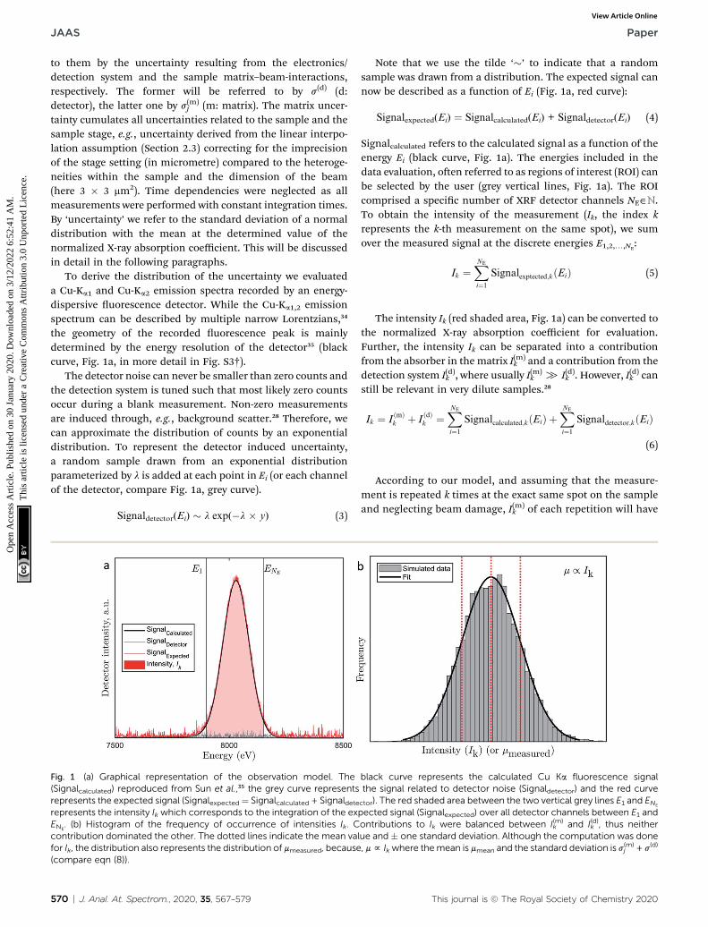
The detector noise can never be smaller than zero counts andthe detection system is tuned such that most likely zero countsoccur during a blank measurement. Non-zero measurementsare induced through, e.g., background scatter.28 Therefore, wecan approximate the distribution of counts by an exponentialdistribution. To represent the detector induced uncertainty,a random sample drawn from an exponential distributionparameterized by l is added at each point in Ei (or each channelof the detector, compare Fig. 1a, grey curve).

Signaldetector(Ei) � l exp(�l � y) (3)

Fig. 1 (a) Graphical representation of the observation model. The(Signalcalculated) reproduced from Sun et al.,35 the grey curve representsrepresents the expected signal (Signalexpected ¼ Signalcalculated + Signaldeterepresents the intensity Ik which corresponds to the integration of the exENE

. (b) Histogram of the frequency of occurrence of intensities Ik. Ccontribution dominated the other. The dotted lines indicate the mean vafor Ik, the distribution also represents the distribution of mmeasured, because(compare eqn (8)).


Note that we use the tilde ‘�’ to indicate that a randomsample was drawn from a distribution. The expected signal cannow be described as a function of Ei (Fig. 1a, red curve):

Signalexpected(Ei) ¼ Signalcalculated(Ei) + Signaldetector(Ei) (4)

Signalcalculated refers to the calculated signal as a function of theenergy Ei (black curve, Fig. 1a). The energies included in thedata evaluation, oen referred to as regions of interest (ROI) canbe selected by the user (grey vertical lines, Fig. 1a). The ROIcomprised a specic number of XRF detector channels NE˛ℕ.To obtain the intensity of the measurement (Ik, the index krepresents the k-th measurement on the same spot), we sumover the measured signal at the discrete energies E1,2,.,NE

:

Ik ¼XNE

i¼1

Signalexptected;kðEiÞ (5)

The intensity Ik (red shaded area, Fig. 1a) can be converted tothe normalized X-ray absorption coefficient for evaluation.Further, the intensity Ik can be separated into a contributionfrom the absorber in the matrix I(m)

k and a contribution from thedetection system I(d)k , where usually I(m)

k [ I(d)k . However, I(d)k canstill be relevant in very dilute samples.28

Ik ¼ IðmÞk þ I

ðdÞk ¼

XNE

i¼1

Signalcalculated;kðEiÞ þXNE

i¼1

Signaldetector;kðEiÞ

(6)

According to our model, and assuming that the measure-ment is repeated k times at the exact same spot on the sampleand neglecting beam damage, I(m)

k of each repetition will have

black curve represents the calculated Cu Ka fluorescence signalthe signal related to detector noise (Signaldetector) and the red curve

ctor). The red shaded area between the two vertical grey lines E1 and ENE

pected signal (Signalexpected) over all detector channels between E1 andontributions to Ik were balanced between I(m)

k and I(d)k , thus neitherlue and � one standard deviation. Although the computation was done, mf Ikwhere themean is mmean and the standard deviation is s(m)

j + s(d)





Paper JAAS

Ope

n A

cces

s A

rtic

le. P

ublis

hed

on 3

0 Ja

nuar

y 20

20. D

ownl

oade

d on

3/1

2/20

22 6

:52:

41 A

M.

Thi

s ar

ticle

is li

cens

ed u

nder

a C

reat

ive

Com

mon

s A

ttrib

utio

n 3.

0 U

npor

ted

Lic

ence


the exact same value (uorescence is a stochastic process aswell, however its variance is small compared to the processesdiscussed further down and not considered here). In contrast,I(d)k (contains stochastic and electronic noise) will vary slightlyas this value was sampled from an exponential distribution ineach detector bin. In practice, however, the monochromator isset to a specic energy and the stage is moved with a givenvelocity line by line. Ik is obtained by integrating the signalover a selected time period. The ‘width’ of a pixel is calculatedas the product of the scan speed and the integration time(nstageDtintegration ¼Wpixel). Aer completion of one XRF map ata certain energy, the energy is changed and an additional XRFmap is recorded, etc. Ideally, the stage should be located at theexact same position at time t for every energy map. However,the locations of the stage will vary slightly, and even thesmallest deviations between positions of consecutive energymaps will result in different ‘absorber environments’ ofa specic location (pixel) at different energies. These differ-ences, unfortunately, cannot be corrected entirely (Section2.3). This situation is comparable to XAS at standard XASbeamlines at advanced synchrotron facilities with beamextensions of a few hundreds of micrometres, where the X-raybeam may slightly shi or change spatial ux density asa function of the energy and even tiny heterogeneities,diffraction artefacts or ‘pinholes’ in the sample can distort theabsorption spectrum.

Furthermore, minor variations in I(m)k may arise from, e.g.,

resonant X-ray inelastic scattering (RIXS) at the absorber orelastic and inelastic scattering at any matrix element.28,36,37 InRIXS, the splitting of the photon emission energy at pre-edgeenergies of conventional XANES measurements as previouslyobserved for CuO36 may eventually increase the uncertainty inthe pre-edge region. However, the distortion introduced by theRIXS contributions is small compared to the intensity of theabsorption edge and further obscured by the energy resolutionof the XRF detector.35,38 The removal of spectra distorted withcontributions from elastic and inelastic scattering is discussedin Section 2.7. Differently, the change in the mean X-ray pene-tration depth before and aer the absorption edge at spots withstrong absorber concretions that extend into the Z direction,e.g., over the total thin section height, might articially enhancethe contribution of the XRF intensity on the low energy side ofthe edge. This may be important, especially if the speciationchanges in Z direction.

The resulting distribution of Ik to some extent depends onthe assumption for the variation of I(m)

k . However, the tendencytowards a normal distribution is imposed by the variation ofI(d)k . The spatial deviations of the stage position from theintended position between consecutive energy maps can beapproximated by a normal distribution indicating a close tozero mean displacement (7 � 10�7 mm) and a standard devia-tion of 3 � 10�4 mm (Fig. S2†). Thus, for 95% of all pixels, thedisplacement is less than 1/2300 of the side length of a pixel.However, X-ray absorption is extremely sensitive to the absorberconcentration and coordination. Therefore, larger displace-ments from the exact location of the pixel relative to the beaminduce larger uncertainties. This consideration qualies the


selection of a normal distribution to describe the uncertainty inI(m)k . Also, a normal distribution is most suitable to capture thesum of all uncertainties of the processes that were deemedrelevant previously but cannot be assessed in detail. 28 In plainlanguage, the size of the area underneath the black curvebetween the grey horizontal lines is sampled from a normaldistribution (Fig. 1a). The result of the listed effects can beillustrated if k¼ 1,2,., 104 synthetic replicate measurements atone pixel are simulated and one arrives at another normaldistribution (Fig. 1b).

By collecting sufficient repetitions of I(m)k + I(d)k , the mean of Ik

and sum of two parameters s(m)j and s(d) can be obtained (red

dotted lines, Fig. 1b). These describe the most likely and meanvalues of the uncertainty introduced by different elements of thebeamline. The uncertainty s(m)

j will be different for each map j,but s(d) will be the same as long as the experimental setupremains unaltered. The uncertainty in the X-ray absorptioncoefficient (m) can be derived as outlined below.

mfIk

I0fIk (7)

The value of I0 is obtained using an ion chamber and thusthe uncertainty in the measurement of I0 is very small and canthus be neglected here. Due to the linear relationship between m

and Ik the uncertainty in m can also be described by a normaldistribution. Thus, any measured normalized X-ray absorptioncoefficient (mmeasured) can be sampled from a normal distribu-tion (N) where the mean is the corresponding, (presumably)true normalized X-ray absorption coefficient (mmean) and thestandard deviation reects the sum of the normalized uncer-tainties introduced by the matrix and the detector:

mmeasured � N(mmean, [s(m)j + s(d)]). (8)

Eqn (8) indicates that the total uncertainty (s(m)j + s(d)) is an

absolute quantity. However, in the present study, the X-rayabsorption coefficients m were normalized to values between0 and 1, hence uncertainties obtained for different datasets arecomparable.

Due to practical constraints (e.g. available beam time, beamdamage), XRF maps at a given energy were only recorded once.This, however, hampers the determination of the measurementuncertainty through assessing the standard deviations. Conse-quently, we cannot determine the uncertainty directly related tothe XRF intensities, only the uncertainty relative to a LCF result.Therefore, a proper choice of spectra from referencematerials iscritical for capturing the XAS signal originating from Cu speciesin the sample (compare Section 2.4 and eqn (1)). In this section,we argued that the uncertainty related to XRF signal productionis comparable for each XRF measurement at every energy for allpixels. Thus, Bayesian inference can be used to evaluate theuncertainties according to eqn (8). We performedMarkov ChainMonte Carlo (MC) Simulations using JAGS (“Just Another GibbsSampler”) Version 4.3.0, based on BUGS (“Bayesian inferenceUsing Gibbs Sampling”),39 through the R library “rjags”40 inRStudio Version 1.1.456 under R Version 3.4.4 (ref. 41) to





JAAS Paper

Ope

n A

cces

s A

rtic

le. P

ublis

hed

on 3

0 Ja

nuar

y 20

20. D

ownl

oade

d on

3/1

2/20

22 6

:52:

41 A

M.

Thi

s ar

ticle

is li

cens

ed u

nder

a C

reat

ive

Com

mon

s A

ttrib

utio

n 3.

0 U

npor

ted

Lic

ence


quantify s(m)j and s(d). Details of the computation and the

computer code are available in the ESI (Section S5†). Briey, inthe MC, the standard deviations s(m)

j and s(d) (eqn (8)) aretreated as two normal distribution that are each characterizedby a mean and standard deviation, which are to be determined(eqn S3 and S4†).

2.6 Synthetic data for model testing and calibration of thedata interpretability

For model testing a synthetic dataset was prepared that covereda large variety of combinations of the six reference spectra. Foreach synthetic dataset, we created 1000 pixels (measurementsor data points) where the (input) fractions were sampled froma Dirichlet distribution.

Xn

i¼1

xi ¼ 1 with cxi $ 0 (9)

A linear combination reconstruction of the normalized X-rayabsorption coefficient was performed (eqn (1) without 3) atthe seven energies at which XRF maps were recorded (Fig. S1†).Finally, the normalized X-ray absorption coefficients weremodied by the introduction of variable magnitudes of noiseaccording to eqn (8).

2.7 Quality criteria and benchmarking

Fit quality benchmarking was performed using the previouslydescribed synthetic datasets augmented with specic quantitiesof uncertainty (noise) (Fig. S7†). Thereaer, LCFs were per-formed to each pixel in each dataset, resulting in output frac-tions. The larger the uncertainty added to a dataset, the lagerthe expected discrepancy between the input and the outputfractions. The generated input fractions of each data point(pixel) were sorted by their weight and compared to thecomputed output fractions, which were equally sorted. A scoreranging from 0 to 6 was assigned to each pixel reecting theagreement between the sorted input and the output fractions. Azero means that the rst (largest) fractions is wrongly assigned,an one means that the largest fraction is correctly assigned, etc.Finally, a six means that the fractions of the reference spectraused for the LCF ts decreased in the same order for the input

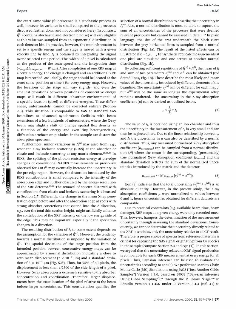
Fig. 2 The introduced uncertainty (x-axis) versus the recovered uncertaexperiment. Each shade of grey is associated with one replicate. In each[0, 0.01, 0.1, 0.2] were recovered for four times 1000 pixels. The horizos(m)3 and s(d) ¼ 0.10 and s(m)

4 ¼ 0.20.


and for the output fractions. The scores of the total dataset werethen averaged. Furthermore, the percentage of pixels wascalculated, for which the reference spectra with the largestspectral component (reference material spectrum) contributingto the LCF t was correctly identied (score$ 1). The scores andthe percentage of pixels (Correct largest Spectral ComponentIdentied: CSCI) as described above can be used to assess thequality of the ts at different levels of uncertainty. Arguments inthe favour of the introduction of the score and CSCI are given inthe ESI (Section S6†).

3 Results and discussion3.1 Validation of the uncertainty analysis technique

3.1.1 Recovery of the uncertainty from synthetic data. Asynthetic dataset with four times 1000 pixels (or spectra) wascompiled according to Section 2.6 with s(d) ¼ 0.1 and s(m)

j ¼ [0,0.01, 0.1, 0.2]. In this way, 1000 pixels contained an uncertaintyof s(d) + s(m)

1 ¼ 0.1 + 0 ¼ 0.1, the following 1000 pixels of s(d) +s(m)2 ¼ 0.1 + 0.01 ¼ 0.11, etc. Distributions of the noise (s(m)

j ands(d)) and the LCF fractions of reference materials (~xi) wererecovered with the MC approach by sampling 103 times fromthe model per pixel aer initiating the model for 2 � 103 iter-ations. The long initiation phase ensured sampling underconstant conditions. With this approach, the introduceduncertainties in synthetic spectra were successfully reproduced(Fig. 2), although the recovered values for the noise were slightlyhigher compared to the noise in the synthetic dataset (z5%).Also, a correlation between s(d) and s(m)

j was evident: lowervalues of s(d) led to higher values of s(m)

j and vice versa (Fig. S8†).This is caused by the linear dependence of these two parame-ters, which add up to the same uncertainty (eq. (8)). Asa consequence, all s(m)

j and s(d) were subsequently combined tos(d) + s(m)

j ¼ sj. Recovering sj from four additional datasets withsj ¼ [0, 0.01, 0.1, 0.2] during 10 repetitions yielded sj ¼ [0.0014� 8 � 10�4, 0.0103 � 10�4, 0.0988 � 2 � 10�4, 0.2032 � 5 �10�4]. The standard error varied between 1.87 � 10�3 and 1.38� 10�2. These results demonstrate that our approach recoversuncertainties in the synthetic dataset with high precision(standard error # 1.4%) and accuracy (relative deviation #

1.6%). The dataset sj ¼ 0 was not included in the evaluation of

inty (y-axis). Data shown are the result of ten replicates of the identicalreplicate experiment, the introduced uncertainties s(d) ¼ 0.1 and s(m)

j ¼ntal, dotted lines indicate the introduced uncertainties of s(m)

2 ¼ 0.01,





Paper JAAS

Ope

n A

cces

s A

rtic

le. P

ublis

hed

on 3

0 Ja

nuar

y 20

20. D

ownl

oade

d on

3/1

2/20

22 6

:52:

41 A

M.

Thi

s ar

ticle

is li

cens

ed u

nder

a C

reat

ive

Com

mon

s A

ttrib

utio

n 3.

0 U

npor

ted

Lic

ence


the accuracy of the uncertainty as relative deviations weredifficult to calculate.

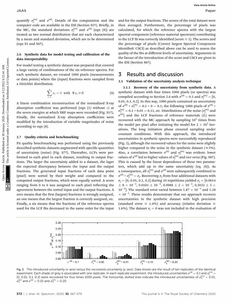
3.1.2 Recovery of the input fractions from synthetic data.In this section the recovery of the correct spectral componentsof the synthetic XAS spectra with a well-dened uncertaintyranging from 0 to 0.20 (sj, levels according to Fig. 3 abscissaand Table S1†) were evaluated. The procedure follows thepreviously discussed workow (Sections 2.6 and 2.7, outlinedin Fig. S7†). In the absence of noise, and using the samereference spectra as in the synthetic data, the score reached1.742 and the CSCI was 72.4% of the pixels (Fig. 3a and b,black circles). Performing LCF using a sequential quadraticprogramming (sqp) method42,43 (implemented through thefunction fmincon in Matlab, only constraint: cxi $ 0) thescore for the noise-free data increased to about 3 (Fig. 3, blacktriangles) but the CSCI decreased to about 60%. Othercommonly used algorithms, e.g., simplex,44 yielded muchlower scores (data not shown). At noise levels in the syntheticspectra of 0.01 or higher, the scores and CSCI values resultingfrom the MC approach and the sqp method were almostidentical (Fig. 3). However, both the score (a) and the CSCI (b)exponentially decreased with increasing noise. Due to thesimilarity of the Cu(II)–O spectra (tenorite, cuprospinel andcopper sulphate) and the Cu–S spectra, (covellite, chalcopy-rite and the amorphous cupper sulphide45), the respectivespectra were treated interchangeably and referred to as‘Cu(II)–O’ and ‘Cu–S’ combined. Through this procedure, thescores and the CSCIs signicantly increased (Fig. 3). Althoughthe score still showed a decreasing trend with increasinguncertainty, it remained above 1.5 at the highest uncertainty(s ¼ 0.2). Comparable results were observed to the CSCI, andin around 70% of all ‘measurements’, the most importantspectral component was identied correctly. This indicatesthat the quality of the spectra allow to discriminate betweenCu(II)–O and Cu–S species in the experimental samples,however, a further differentiation into individual Cu(II)–O andCu–S species may not be possible. To some extent this isrelated to the spectral similarity of different Cu(II)–O/Cu–S

Fig. 3 (a) The score (number of correct fractions/pixel) and (b) CSCI (Cintroduced to the data. Black lines indicate that each referencewas treatewas treated as interchangeable as discussed in the text. Circles indicatetriangles represent data determined using sequential quadratic program


reference materials which may be compensated by recordingadditional XRF maps at different energies. We propose to usethe described procedure to evaluate expected score/CSCIs atvariable energies and levels of uncertainties when planningsynchrotron chemical imaging experiments.

3.2 The uncertainty in the case study datasets

The uncertainties in four experimental datasets recorded ondigested sewage sludge spiked with CuO-NP or CuSO4 and theresulting ashes were assessed using the approach describedabove. The levels of uncertainty were then compared to those inSection 3.1.2 and information on the quality of the extractedLCF ts were obtained. Briey, XRF maps of the CuO spikedsludge (SLG NP), the CuSO4 spiked sludge (SLG AQ) and ashderived from SLG AQ (ASH AQ) were 500 � 500 mm2 in size witha 3 mm lateral resolution. The map of the ash derived from SLGNP (ASH NP) was 350 � 350 mm2 with the same lateralresolution.

For initial and comparative analyses, all pixels with a non-normalized (NN) post edge XRF intensity of at least threetimes the NN pre-edge XRF intensity were included in theanalysis. The correlation between s(m)

j and s(d), previouslyobserved in the synthetic data, was also observed in the exper-imental data (Fig. S9†). Therefore, we combined these uncer-tainties into sj(s

(d) + s(m)j ¼ sj) and found sj ¼ [0.18, 0.17, 0.13,

0.33] for the experimental datasets SLG NP, SLG AQ, ASH NPand ASH AQ, respectively (Fig. S10†). Similar to the analysis ofthe synthetic datasets, the uncertainty was represented bya normal distribution around the values of sj. The uncertaintyestimated for the two sludge samples was almost identical,likely due to the comparable sample matrix and Cu concentra-tions. The larger sj of ASH AQ may be explained by the granulartexture of the ASH AQ sample resulting in an investigated area,dominated by an ash grain with rather low Cu concentrations.

Based on the results obtained with the synthetic dataset,uncertainties in the range of 0.13–0.18 as obtained for theexperimental dataset translate into Cu(II)–O and Cu–Scombined scores of around 1.5 and CSCI between 65 and

orrect largest Spectral Component Identified) versus the uncertaintyd individually, grey lines indicate that each Cu(II)–O and Cu–S referencethat the score and CSCI was determined using the Markov Chain (MC),ming (sqp).





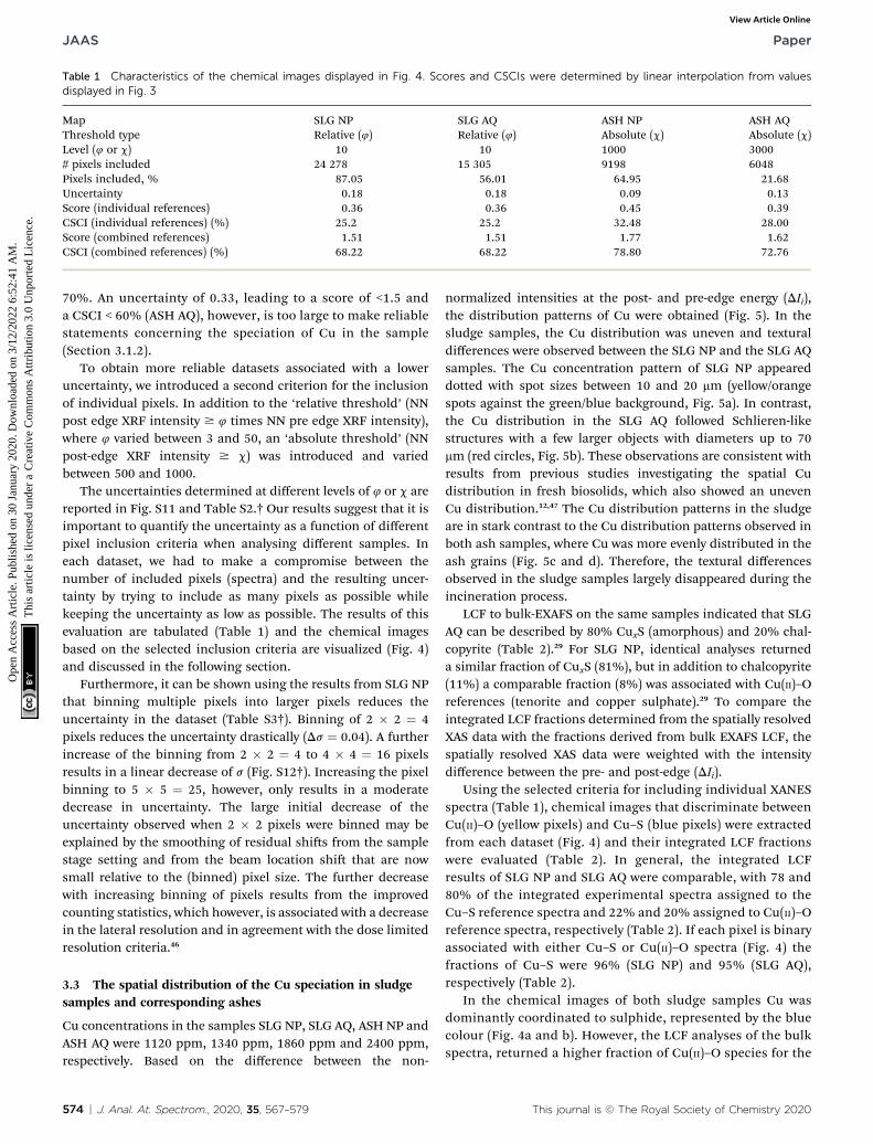
Table 1 Characteristics of the chemical images displayed in Fig. 4. Scores and CSCIs were determined by linear interpolation from valuesdisplayed in Fig. 3

Map SLG NP SLG AQ ASH NP ASH AQThreshold type Relative (4) Relative (4) Absolute (c) Absolute (c)Level (4 or c) 10 10 1000 3000# pixels included 24 278 15 305 9198 6048Pixels included, % 87.05 56.01 64.95 21.68Uncertainty 0.18 0.18 0.09 0.13Score (individual references) 0.36 0.36 0.45 0.39CSCI (individual references) (%) 25.2 25.2 32.48 28.00Score (combined references) 1.51 1.51 1.77 1.62CSCI (combined references) (%) 68.22 68.22 78.80 72.76

JAAS Paper

Ope

n A

cces

s A

rtic

le. P

ublis

hed

on 3

0 Ja

nuar

y 20

20. D

ownl

oade

d on

3/1

2/20

22 6

:52:

41 A

M.

Thi

s ar

ticle

is li

cens

ed u

nder

a C

reat

ive

Com

mon

s A

ttrib

utio

n 3.

0 U

npor

ted

Lic

ence


70%. An uncertainty of 0.33, leading to a score of <1.5 anda CSCI < 60% (ASH AQ), however, is too large to make reliablestatements concerning the speciation of Cu in the sample(Section 3.1.2).

To obtain more reliable datasets associated with a loweruncertainty, we introduced a second criterion for the inclusionof individual pixels. In addition to the ‘relative threshold’ (NNpost edge XRF intensity $ 4 times NN pre edge XRF intensity),where 4 varied between 3 and 50, an ‘absolute threshold’ (NNpost-edge XRF intensity $ c) was introduced and variedbetween 500 and 1000.

The uncertainties determined at different levels of 4 or c arereported in Fig. S11 and Table S2.† Our results suggest that it isimportant to quantify the uncertainty as a function of differentpixel inclusion criteria when analysing different samples. Ineach dataset, we had to make a compromise between thenumber of included pixels (spectra) and the resulting uncer-tainty by trying to include as many pixels as possible whilekeeping the uncertainty as low as possible. The results of thisevaluation are tabulated (Table 1) and the chemical imagesbased on the selected inclusion criteria are visualized (Fig. 4)and discussed in the following section.

Furthermore, it can be shown using the results from SLG NPthat binning multiple pixels into larger pixels reduces theuncertainty in the dataset (Table S3†). Binning of 2 � 2 ¼ 4pixels reduces the uncertainty drastically (Ds ¼ 0.04). A furtherincrease of the binning from 2 � 2 ¼ 4 to 4 � 4 ¼ 16 pixelsresults in a linear decrease of s (Fig. S12†). Increasing the pixelbinning to 5 � 5 ¼ 25, however, only results in a moderatedecrease in uncertainty. The large initial decrease of theuncertainty observed when 2 � 2 pixels were binned may beexplained by the smoothing of residual shis from the samplestage setting and from the beam location shi that are nowsmall relative to the (binned) pixel size. The further decreasewith increasing binning of pixels results from the improvedcounting statistics, which however, is associated with a decreasein the lateral resolution and in agreement with the dose limitedresolution criteria.46

3.3 The spatial distribution of the Cu speciation in sludgesamples and corresponding ashes

Cu concentrations in the samples SLG NP, SLG AQ, ASH NP andASH AQ were 1120 ppm, 1340 ppm, 1860 ppm and 2400 ppm,respectively. Based on the difference between the non-


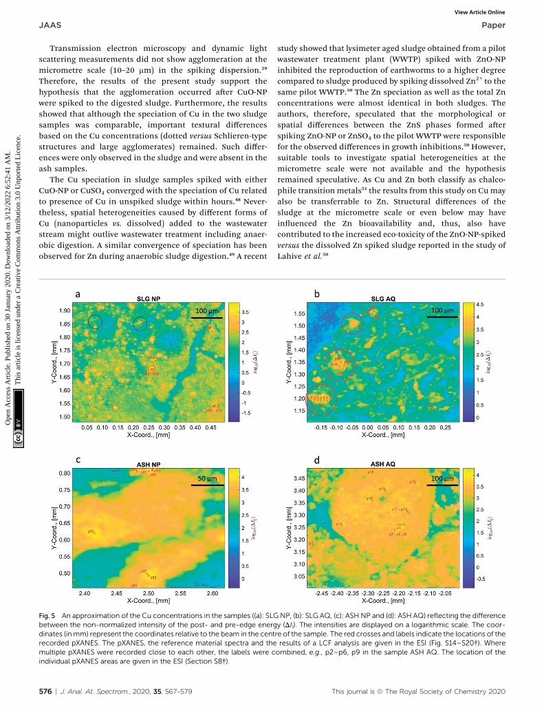
normalized intensities at the post- and pre-edge energy (DIi),the distribution patterns of Cu were obtained (Fig. 5). In thesludge samples, the Cu distribution was uneven and texturaldifferences were observed between the SLG NP and the SLG AQsamples. The Cu concentration pattern of SLG NP appeareddotted with spot sizes between 10 and 20 mm (yellow/orangespots against the green/blue background, Fig. 5a). In contrast,the Cu distribution in the SLG AQ followed Schlieren-likestructures with a few larger objects with diameters up to 70mm (red circles, Fig. 5b). These observations are consistent withresults from previous studies investigating the spatial Cudistribution in fresh biosolids, which also showed an unevenCu distribution.12,47 The Cu distribution patterns in the sludgeare in stark contrast to the Cu distribution patterns observed inboth ash samples, where Cu was more evenly distributed in theash grains (Fig. 5c and d). Therefore, the textural differencesobserved in the sludge samples largely disappeared during theincineration process.

LCF to bulk-EXAFS on the same samples indicated that SLGAQ can be described by 80% CuxS (amorphous) and 20% chal-copyrite (Table 2).29 For SLG NP, identical analyses returneda similar fraction of CuxS (81%), but in addition to chalcopyrite(11%) a comparable fraction (8%) was associated with Cu(II)–Oreferences (tenorite and copper sulphate).29 To compare theintegrated LCF fractions determined from the spatially resolvedXAS data with the fractions derived from bulk EXAFS LCF, thespatially resolved XAS data were weighted with the intensitydifference between the pre- and post-edge (DIi).

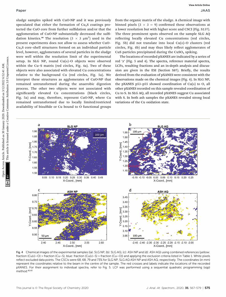
Using the selected criteria for including individual XANESspectra (Table 1), chemical images that discriminate betweenCu(II)–O (yellow pixels) and Cu–S (blue pixels) were extractedfrom each dataset (Fig. 4) and their integrated LCF fractionswere evaluated (Table 2). In general, the integrated LCFresults of SLG NP and SLG AQ were comparable, with 78 and80% of the integrated experimental spectra assigned to theCu–S reference spectra and 22% and 20% assigned to Cu(II)–Oreference spectra, respectively (Table 2). If each pixel is binaryassociated with either Cu–S or Cu(II)–O spectra (Fig. 4) thefractions of Cu–S were 96% (SLG NP) and 95% (SLG AQ),respectively (Table 2).

In the chemical images of both sludge samples Cu wasdominantly coordinated to sulphide, represented by the bluecolour (Fig. 4a and b). However, the LCF analyses of the bulkspectra, returned a higher fraction of Cu(II)–O species for the





Paper JAAS

Ope

n A

cces

s A

rtic

le. P

ublis

hed

on 3

0 Ja

nuar

y 20

20. D

ownl

oade

d on

3/1

2/20

22 6

:52:

41 A

M.

Thi

s ar

ticle

is li

cens

ed u

nder

a C

reat

ive

Com

mon

s A

ttrib

utio

n 3.

0 U

npor

ted

Lic

ence


sludge samples spiked with CuO-NP and it was previouslyspeculated that either the formation of CuxS coatings pro-tected the CuO core from further suldation and/or that theagglomeration of CuO-NP substantially decreased the sul-dation kinetics.48 The resolution (3 � 3 mm2) used in thepresent experiments does not allow to assess whether CuO–CuxS core–shell structures formed on an individual particlelevel, however, agglomerates of several particles in the sludgewere well within the resolution limit of the experimentalsetup. In SLG NP, round Cu(II)–O objects were observedwithin the Cu–S matrix (red circles, Fig. 4a). Two of theseobjects were also associated with elevated Cu concentrationsrelative to the background Cu (red circles, Fig. 5a). Weinterpret these structures as agglomerates of CuO-NP thatremained untransformed during the anaerobic digestionprocess. The other two objects were not associated withsignicantly elevated Cu concentrations (black circles,Fig. 5a) and may, therefore, represent CuO-NP, where Curemained untransformed due to locally limited/restrictedavailability of bisulde or Cu bound to O functional groups

Fig. 4 Chemical images of the experimental samples ((a): SLG NP, (b): SLfraction (Cu(II)–O) > fraction (Cu–S), blue: fraction (Cu(II)–S) > fraction (Creflect excluded data points. The CSCIs were 68, 68, 79 and 73% for SLG Nrepresent the coordinates relative to the beam in the centre of the sampXANES. For their assignment to individual spectra, refer to Fig. 5. Lmethod.42,43


from the organic matrix of the sludge. A chemical image withbinned pixels (3 � 3 ¼ 9) conrmed these observations ata lower resolution but with higher score and CSCI (Fig. S13†).The three prominent spots observed on the sample SLG AQreecting locally elevated Cu concentrations (red circles,Fig. 5b) did not translate into local Cu(II)–O clusters (redcircles, Fig. 4b) and may thus likely reect agglomerates ofCuS particles precipitated during the CuSO4 spiking.

The locations of recorded pXANES are indicated by a series ofred ‘x’ (Fig. 5 and 4). The spectra, reference material spectra,LCFs, resulting fractions and an in-depth analysis and discus-sion are given in the ESI (Section S8†). Briey, the resultsderived from the evaluation of pXANES were consistent with theobservations made on the chemical images (Fig. 4). In SLG NP,the pXANES p53–p55 showed coordination of Cu(II) to O, allother pXANES recorded on this sample revealed coordination ofCu to S. In SLG AQ, all recorded pXANES suggest Cu associatedwith S. In both ash samples the pXANES revealed strong localvariations of the Cu oxidation state.

G AQ, (c): ASH NP and (d): ASH AQ) using combined references (yellow:u–O)) and applying the exclusion criteria listed in Table 1. White pixelsP, SLG AQ ASH NP and ASH AQ, respectively. The coordinates (in mm)ple. The red crosses and labels indicate the locations of the recordedCF was performed using a sequential quadratic programming (sqp)





JAAS Paper

Ope

n A

cces

s A

rtic

le. P

ublis

hed

on 3

0 Ja

nuar

y 20

20. D

ownl

oade

d on

3/1

2/20

22 6

:52:

41 A

M.

Thi

s ar

ticle

is li

cens

ed u

nder

a C

reat

ive

Com

mon

s A

ttrib

utio

n 3.

0 U

npor

ted

Lic

ence


Transmission electron microscopy and dynamic lightscattering measurements did not show agglomeration at themicrometre scale (10–20 mm) in the spiking dispersion.29

Therefore, the results of the present study support thehypothesis that the agglomeration occurred aer CuO-NPwere spiked to the digested sludge. Furthermore, the resultsshowed that although the speciation of Cu in the two sludgesamples was comparable, important textural differencesbased on the Cu concentrations (dotted versus Schlieren-typestructures and large agglomerates) remained. Such differ-ences were only observed in the sludge and were absent in theash samples.

The Cu speciation in sludge samples spiked with eitherCuO-NP or CuSO4 converged with the speciation of Cu relatedto presence of Cu in unspiked sludge within hours.48 Never-theless, spatial heterogeneities caused by different forms ofCu (nanoparticles vs. dissolved) added to the wastewaterstream might outlive wastewater treatment including anaer-obic digestion. A similar convergence of speciation has beenobserved for Zn during anaerobic sludge digestion.49 A recent

Fig. 5 An approximation of the Cu concentrations in the samples ((a): SLGbetween the non-normalized intensity of the post- and pre-edge energdinates (inmm) represent the coordinates relative to the beam in the centrecorded pXANES. The pXANES, the reference material spectra and themultiple pXANES were recorded close to each other, the labels were cindividual pXANES areas are given in the ESI (Section S8†).


study showed that lysimeter aged sludge obtained from a pilotwastewater treatment plant (WWTP) spiked with ZnO-NPinhibited the reproduction of earthworms to a higher degreecompared to sludge produced by spiking dissolved Zn2+ to thesame pilot WWTP.50 The Zn speciation as well as the total Znconcentrations were almost identical in both sludges. Theauthors, therefore, speculated that the morphological orspatial differences between the ZnS phases formed aerspiking ZnO-NP or ZnSO4 to the pilot WWTP were responsiblefor the observed differences in growth inhibitions.50 However,suitable tools to investigate spatial heterogeneities at themicrometre scale were not available and the hypothesisremained speculative. As Cu and Zn both classify as chalco-phile transition metals51 the results from this study on Cumayalso be transferrable to Zn. Structural differences of thesludge at the micrometre scale or even below may haveinuenced the Zn bioavailability and, thus, also havecontributed to the increased eco-toxicity of the ZnO-NP-spikedversus the dissolved Zn spiked sludge reported in the study ofLahive et al.50

NP, (b): SLG AQ, (c): ASH NP and (d): ASH AQ) reflecting the differencey (DIi). The intensities are displayed on a logarithmic scale. The coor-re of the sample. The red crosses and labels indicate the locations of theresults of a LCF analysis are given in the ESI (Fig. S14–S20†). Where

ombined, e.g., p2–p6, p9 in the sample ASH AQ. The location of the





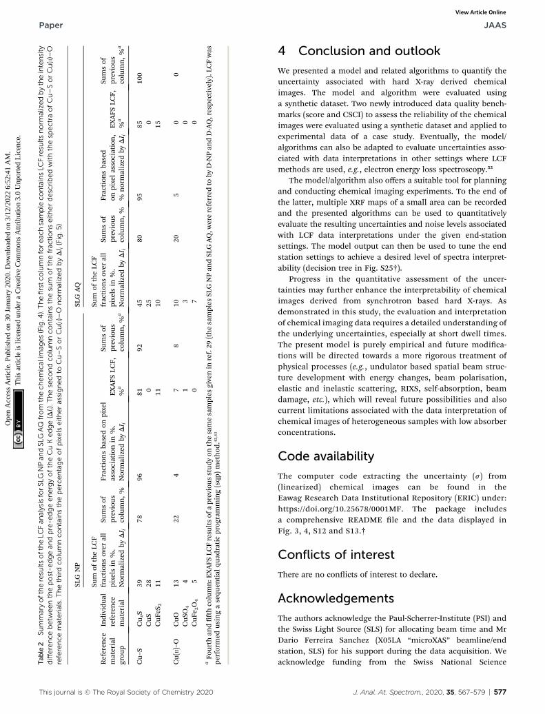
Tab

le2

Summaryoftheresu

ltsoftheLC

Fan

alysisforSL

GNPan

dSL

GAQ

from

thech

emicalim

ages(Fig.4

).Thefirstco

lumnforeac

hsample

containsLC

Fresu

ltsnorm

alizedbytheintensity

difference

betw

eenthepost-e

dgean

dpre-e

dgeenergyoftheCuKedge(DI i).T

heseco

ndco

lumnco

ntainsthesu

mofthefrac

tionseitherdescribedwiththesp

ectra

ofCu–SorCu(II)–O

reference

materials.Thethirdco

lumnco

ntainsthepercentageofpixelseitherassignedto

Cu–SorCu( II)–O

norm

alizedbyDI i(Fig.5

)

Referen

cematerial

grou

p

Individua

lreference

material

SLGNP

SLGAQ

Sum

oftheLC

Ffraction

sover

all

pixels

in%.

Normalized

byDI i

Sumsof

previous

column,%

Fraction

sba

sedon

pixel

associationin

%.

Normalized

byDI i

EXAFS

LCF,

%a

Sumsof

previous

column,%

a

Sum

oftheLC

Ffraction

sover

all

pixels

in%.

Normalized

byDI i

Sumsof

previous

column,%

Fraction

sba

sed

onpixelassociation,

%normalized

byDI i

EXAFS

LCF,

%a

Sumsof

previous

column,%

a

Cu–

SCu xS

3978

9681

9245

8095

8510

0CuS

280

250

CuF

eS2

1111

1015

Cu( II)–O

CuO

1322

47

810

205

00

CuSO

44

13

0CuF

e 2O4

50

70

aFo

urth

andhcolumn:E

XAFS

LCFresu

ltsof

aprevious

stud

yon

thesamesamples

givenin

ref.29

(thesamples

SLGNPan

dSL

GAQ,w

erereferred

toby

D-NPan

dD-AQ,respe

ctively).L

CFwas

performed

usingasequ

ential

quad

raticprog

ramming(sqp

)method

.42,43


Paper JAAS

Ope

n A

cces

s A

rtic

le. P

ublis

hed

on 3

0 Ja

nuar

y 20

20. D

ownl

oade

d on

3/1

2/20

22 6

:52:

41 A

M.

Thi

s ar

ticle

is li

cens

ed u

nder

a C

reat

ive

Com

mon

s A

ttrib

utio

n 3.

0 U

npor

ted

Lic

ence


4 Conclusion and outlook

We presented a model and related algorithms to quantify theuncertainty associated with hard X-ray derived chemicalimages. The model and algorithm were evaluated usinga synthetic dataset. Two newly introduced data quality bench-marks (score and CSCI) to assess the reliability of the chemicalimages were evaluated using a synthetic dataset and applied toexperimental data of a case study. Eventually, the model/algorithms can also be adapted to evaluate uncertainties asso-ciated with data interpretations in other settings where LCFmethods are used, e.g., electron energy loss spectroscopy.52

The model/algorithm also offers a suitable tool for planningand conducting chemical imaging experiments. To the end ofthe latter, multiple XRF maps of a small area can be recordedand the presented algorithms can be used to quantitativelyevaluate the resulting uncertainties and noise levels associatedwith LCF data interpretations under the given end-stationsettings. The model output can then be used to tune the endstation settings to achieve a desired level of spectra interpret-ability (decision tree in Fig. S25†).

Progress in the quantitative assessment of the uncer-tainties may further enhance the interpretability of chemicalimages derived from synchrotron based hard X-rays. Asdemonstrated in this study, the evaluation and interpretationof chemical imaging data requires a detailed understanding ofthe underlying uncertainties, especially at short dwell times.The present model is purely empirical and future modica-tions will be directed towards a more rigorous treatment ofphysical processes (e.g., undulator based spatial beam struc-ture development with energy changes, beam polarisation,elastic and inelastic scattering, RIXS, self-absorption, beamdamage, etc.), which will reveal future possibilities and alsocurrent limitations associated with the data interpretation ofchemical images of heterogeneous samples with low absorberconcentrations.

Code availability

The computer code extracting the uncertainty (s) from(linearized) chemical images can be found in theEawag Research Data Institutional Repository (ERIC) under:https://doi.org/10.25678/0001MF. The package includesa comprehensive README le and the data displayed inFig. 3, 4, S12 and S13.†

Conflicts of interest

There are no conicts of interest to declare.

Acknowledgements

The authors acknowledge the Paul-Scherrer-Institute (PSI) andthe Swiss Light Source (SLS) for allocating beam time and MrDario Ferreira Sanchez (X05LA “microXAS” beamline/endstation, SLS) for his support during the data acquisition. Weacknowledge funding from the Swiss National Science





JAAS Paper

Ope

n A

cces

s A

rtic

le. P

ublis

hed

on 3

0 Ja

nuar

y 20

20. D

ownl

oade

d on

3/1

2/20

22 6

:52:

41 A

M.

Thi

s ar

ticle

is li

cens

ed u

nder

a C

reat

ive

Com

mon

s A

ttrib

utio

n 3.

0 U

npor

ted

Lic

ence


Foundation (SNF) through grant 5221.01038 and as well asdiscretionary funding from Eawag and PSI. Further, weacknowledge the library of ETH Zurich for covering the APC foropen access publishing.

References

1 M. Grafe, E. Donner, R. N. Collins and E. Lombi, Anal. Chim.Acta, 2014, 822, 1–22.

2 D. E. Sayers, E. A. Stern and F. W. Lytle, Phys. Rev. Lett., 1971,27, 1204–1207.

3 E. A. Stern, Phys. Rev. B: Condens. Matter Mater. Phys., 1974,10, 3027–3037.

4 P. Willmott, An introduction to synchrotron radiation:techniques and applications, John Wiley & Sons, 2011.

5 M. A. Marcus, A. A. MacDowell, R. Celestre, A. Manceau,T. Miller, H. A. Padmore and R. E. Sublett, J. SynchrotronRadiat., 2004, 11, 239–247.

6 A. Manceau, N. Tamura, M. A. Marcus, A. A. MacDowell,R. S. Celestre, R. E. Sublett, G. Sposito and H. A. Padmore,Am. Mineral., 2002, 87, 1494–1499.

7 A. Manceau, N. Tamura, R. S. Celestre, A. A. MacDowell,N. Geoffroy, G. Sposito and H. A. Padmore, Environ. Sci.Technol., 2003, 37, 75–80.

8 S. D. Kelly, D. Hesterberg and B. Ravel, Analysis of soils andminerals using X-ray absorption spectroscopy, Methods ofsoil analysis. Part 5, Mineralogical methods, ASA-CSSA-SSSA,5th edn, 2008.

9 A. Lanzirotti, L. Lee, E. Head, S. R. Sutton, M. Newville,M. McCanta, A. H. Lerner and P. J. Wallace, Geochim.Cosmochim. Acta, 2019, 267, 164–178.

10 C. N. Borca, D. Grolimund, M. Willimann, B. Meyer,K. Jemovs, J. Vila-Comamala and C. David, J. Phys.: Conf.Ser., 2009, 186, 012003.

11 R. Kirkham, P. A. Dunn, A. J. Kuczewski, D. P. Siddons,R. Dodanwela, G. F. Moorhead, C. G. Ryan,G. D. Geronimo, R. Beuttenmuller, D. Pinelli, M. Pfeffer,P. Davey, M. Jensen, D. J. Paterson, M. D. d. Jonge,D. L. Howard, M. Kusel and J. McKinlay, AIP Conf. Proc.,2010, 1234, 240–243.

12 B. E. Etschmann, E. Donner, J. Brugger, D. L. Howard,M. D. de Jonge, D. Paterson, R. Naidu, K. G. Scheckel,C. G. Ryan and E. Lombi, Environ. Chem., 2014, 11, 341–350.

13 M. A. Marcus, B. M. Toner and Y. Takahashi, Mar. Chem.,2018, 202, 58–66.

14 J. G. Mesu, A. M. J. van der Eerden, F. M. F. de Groot andB. M. Weckhuysen, J. Phys. Chem. B, 2005, 109, 4042–4047.

15 J. Yang, T. Regier, J. J. Dynes, J. Wang, J. Shi, D. Peak,Y. Zhao, T. Hu, Y. Chen and J. S. Tse, Anal. Chem., 2011,83, 7856–7862.

16 M. A. Marcus, TrAC, Trends Anal. Chem., 2010, 29, 508–517.17 C. M. Rico, M. G. Johnson, M. A. Marcus and C. P. Andersen,

Environ. Sci.: Nano, 2017, 4, 700–711.18 M. I. Heller, P. J. Lam, J. W. Moffett, C. P. Till, J.-M. Lee,

B. M. Toner and M. A. Marcus, Geochim. Cosmochim. Acta,2017, 211, 174–193.


19 P. J. Lam, D. C. Ohnemus and M. A. Marcus, Geochim.Cosmochim. Acta, 2012, 80, 108–124.

20 L. E. Mayhew, S. M. Webb and A. S. Templeton, Environ. Sci.Technol., 2011, 45, 4468–4474.

21 B. M. Toner, S. L. Nicholas and J. K. C. Wasik, Environ.Chem., 2014, 11, 4–9.

22 C. M. Rico, M. G. Johnson and M. A. Marcus, Environ. Sci.:Nano, 2018, 5, 1807–1812.

23 C. G. Ryan, D. P. Siddons, R. Kirkham, P. A. Dunn,A. Kuczewski, G. Moorhead, G. D. Geronimo,D. J. Paterson, M. D. d. Jonge, R. M. Hough, M. J. Lintern,D. L. Howard, P. Kappen and J. Cleverley, AIP Conf. Proc.,2010, 1221, 9–17.

24 E. R. Malinowski, Factor analysis in chemistry, Wiley, 2002.25 E. R. Malinowski, Anal. Chim. Acta, 1978, 103, 339–354.26 A. Manceau, M. Marcus and T. Lenoir, J. Synchrotron Radiat.,

2014, 21, 1140–1147.27 S. Heald, J. Synchrotron Radiat., 2015, 22, 436–445.28 H. Abe, G. Aquilanti, R. Boada, B. Bunker, P. Glatzel,

M. Nachtegaal and S. Pascarelli, J. Synchrotron Radiat.,2018, 25, 972–980.

29 J. Wielinski, A. Gogos, A. Voegelin, C. Muller, E. Morgenrothand R. Kaegi, Environ. Sci. Technol., 2019, 53, 11704–11713.

30 M. Guizar-Sicairos, S. T. Thurman and J. R. Fienup, Opt.Lett., 2008, 33, 156–158.

31 B. Ravel and M. Newville, J. Synchrotron Radiat., 2005, 12,537–541.

32 M. Newville, J. Phys.: Conf. Ser., 2013, 430, 012007.33 S. M. Webb, Phys. Scr., 2005, 2005, 1011.34 M. Deutsch, G. Holzer, J. Hartwig, J. Wolf, M. Fritsch and

E. Forster, Phys. Rev. A, 1995, 51, 283–296.35 Y. Sun, S.-C. Gleber, C. Jacobsen, J. Kirz and S. Vogt,

Ultramicroscopy, 2015, 152, 44–56.36 H. Hayashi, R. Takeda, Y. Udagawa, T. Nakamura,

H. Miyagawa, H. Shoji, S. Nanao and N. Kawamura, Phys.Rev. B: Condens. Matter Mater. Phys., 2003, 68, 045122.

37 H. Hayashi, AIP Conf. Proc., 2007, 882, 833–837.38 P. Glatzel, T.-C. Weng, K. Kvashnina, J. Swarbrick, M. Sikora,

E. Gallo, N. Smolentsev and R. A. Mori, J. Electron Spectrosc.Relat. Phenom., 2013, 188, 17–25.

39 D. J. Lunn, A. Thomas, N. Best and D. Spiegelhalter, Stat.Comput., 2000, 10, 325–337.

40 M. Plummer, JAGS: A program for analysis of Bayesiangraphical models using Gibbs sampling, Proceedings of the3rd international workshop on distributed statisticalcomputing, Vienna, Austria, 2003, vol. 124, No. 125,10, pp.1–10.

41 RCoreTeam, R: A language and environment for statisticalcomputing, R Foundation for Statistical Computing, Vienna,Austria, 2017, https://www.R-project.org/.

42 M. J. Powell, in Numerical analysis, Springer, 1978, pp. 144–157.

43 M. J. Powell, in Nonlinear programming 3, Elsevier, 1978, pp.27–63.

44 J. C. Lagarias, J. A. Reeds, M. H. Wright and P. E. Wright,SIAM J. Optim., 1998, 9, 112–147.





Paper JAAS

Ope

n A

cces

s A

rtic

le. P

ublis

hed

on 3

0 Ja

nuar

y 20

20. D

ownl

oade

d on

3/1

2/20

22 6

:52:

41 A

M.

Thi

s ar

ticle

is li

cens

ed u

nder

a C

reat

ive

Com

mon

s A

ttrib

utio

n 3.

0 U

npor

ted

Lic

ence


45 R. A. D. Pattrick, J. F. W. Mosselmans, J. M. Charnock,K. E. R. England, G. R. Helz, C. D. Garner andD. J. Vaughan, Geochim. Cosmochim. Acta, 1997, 61, 2023–2036.

46 A. Rose, in Advances in Electronics and Electron Physics, ed. L.Marton, Academic Press, 1948, vol. 1, pp. 131–166.

47 E. Donner, D. L. Howard, M. D. d. Jonge, D. Paterson,M. H. Cheah, R. Naidu and E. Lombi, Environ. Sci.Technol., 2011, 45, 7249–7257.

48 A. Gogos, A. Voegelin and R. Kagi, Environ. Sci.: Nano, 2018,5, 2560.


49 E. Lombi, E. Donner, E. Tavakkoli, T. W. Turney, R. Naidu,B. W. Miller and K. G. Scheckel, Environ. Sci. Technol.,2012, 46, 9089–9096.

50 E. Lahive, M. Matzke, M. Durenkamp, A. J. Lawlor,S. A. Thacker, M. G. Pereira, D. J. Spurgeon, J. M. Unrine,C. Svendsen and S. Los, Environ. Sci.: Nano, 2017, 4, 78–88.

51 F. Albarede, in Encyclopedia of Astrobiology, ed. M. Gargaud,R. Amils, J. C. Quintanilla, H. J. Cleaves, W. M. Irvine, D. L.Pinti and M. Viso, Springer Berlin Heidelberg, Berlin,Heidelberg, 2011, pp. 283–283, DOI: 10.1007/978-3-642-11274-4_261.

52 S. Yakovlev and M. Libera, Micron, 2008, 39, 734–740.





Documents

Synchrotron hard X-ray chemical imaging of trace element