Embed Size (px)
Citation preview

Loughborough UniversityInstitutional Repository
Synchronverter-basedcontrol for wind power
This item was submitted to Loughborough University's Institutional Repositoryby the/an author.
Additional Information:
• A Doctoral Thesis. Submitted in partial fulfilment of the requirementsfor the award of Doctor of Philosophy of Loughborough University.
Metadata Record: https://dspace.lboro.ac.uk/2134/10866
Publisher: c© Zhenyu Ma
Please cite the published version.

This item was submitted to Loughborough University as a PhD thesis by the author and is made available in the Institutional Repository
(https://dspace.lboro.ac.uk/) under the following Creative Commons Licence conditions.
For the full text of this licence, please go to: http://creativecommons.org/licenses/by-nc-nd/2.5/
Synchronverter-based Control for Wind Power
by
Zhenyu Ma
A Doctoral thesis
submitted in partial fullment of the requirements for the award of
Doctor of Philosophy
of Loughborough University
July 2012
c© by Zhenyu Ma 2012

Abstract
More and more attention has been paid to the energy crisis due to the increasing energy
demand from industrial and commercial applications. The utilisation of wind power,
which is considered as one of the most promising renewable energy sources, has grown
rapidly in the last three decades. In recent years, many power converter techniques
have been developed to integrate wind power with the electrical grid. The use of power
electronic converters allows for variable speed operation of wind turbines, and enhanced
power extraction. This work, which is supported by EPSRC (Engineering and Physical
Sciences Research Council) and Nheolis under the DHPA (Dorothy Hodgkin Postgrad-
uate Awards) scheme, focuses on the design and analysis of control systems for wind
power.
In this work, two of the most popular AC-DC-AC topologies with PMSG (Per-
manent Magnet Synchronous Generators) have been developed. One consists of an
uncontrollable rectier, a boost converter and an inverter and a current control scheme
is proposed to achieve the MPPT (Maximum Power Point Tracking). In the control
strategy, the output current of the uncontrollable rectier is controlled by a boost con-
verter according to the current reference, which is determined by a climbing algorithm,
to achieve MPPT. The synchronverter technology has been applied to control the in-
verter for the grid-connection. An experimental setup based on DSP (Digital Signal
Processing) has been designed to implement all the above mentioned experiments. In
addition, a synchronverter-based parallel control strategy, which consists of a frequency
droop loop and a voltage droop loop to achieve accurate sharing of real power and re-
active power respectively, has been further studied. Moreover, a control strategy based
on the synchronverter has been presented to force the inverter to have capacitive output
impedance, so that the quality of the output voltage is improved.
The other topology consists of a full-scale back-to-back converter, of which the recti-
er is controllable. Two control strategies have been proposed to operate a three-phase
rectier to mimic a synchronous motor, following the idea of synchronverters to operate
inverters to mimic synchronous generators. In the proposed schemes, the real power
extracted from the source and the output voltage are the control variables, respec-
tively, hence they can be employed in dierent applications. Furthermore, improved
control strategies are proposed to self-synchronise with the grid. This does not only
improve the performance of the system but also considerably reduces the complexity of

the overall controller. All experiments have been implemented on a test rig based on
dSPACE to demonstrate the excellent performance of the proposed control strategies
with unity power factor, sinusoidal currents and good dynamics. Finally, an original
control strategy based on the synchronverter technology has been proposed for back-
to-back converters in wind power applications to make the whole system behave as a
generator-motor-generator system.
3

Acknowledgements
This work has been carried out at the Department of Aeronautical and Automotive
Engineering at Loughborough University and the Department of Electrical Engineering
and Electronics at the University of Liverpool. The nancial support provided by
the Engineering and Physical Sciences Research Council (EPSRC) and the company
Nheolis under the Dorothy Hodgkin Postgraduate Awards (DHPA) scheme is gratefully
acknowledged.
I would like to express my deep gratitude to Prof. Qing-Chang Zhong and Prof.
Wen-Hua Chen for their supervision, valuable discussions and never-ending encourage-
ment, patience and support. This work would not be what it is without their help.
Moreover, I would like to thank Dr. Tomas Hornik for his help in this project, in
particular, on building up the experimental setup. I would also like to thank visiting
scholars and my fellow PhD students: Prof. Fan, Dr. Wang, Dr. Zhang, Dr. Cao,
Long, Shamsul, Max and Olivia for help and discussions regarding my project. And
many thanks to all my colleagues and the sta at the Department of Aeronautical and
Automotive Engineering for the good working atmosphere.
Finally, I would like to thank my family for their support and encouragement
throughout my PhD.

Contents
1 Introduction 1
1.1 Motivation . . . . . . . . . . . . . . . . . . . . . . . . . . . . . . . . . . . 1
1.2 Outline of the Thesis . . . . . . . . . . . . . . . . . . . . . . . . . . . . . 2
1.3 Major Contributions . . . . . . . . . . . . . . . . . . . . . . . . . . . . . 3
1.3.1 Current control for maximum power point tracking . . . . . . . . 3
1.3.2 Rectier control based on synchronverters . . . . . . . . . . . . . 3
1.3.3 Synchronverter-based control in wind power . . . . . . . . . . . . 4
1.4 List of Publications . . . . . . . . . . . . . . . . . . . . . . . . . . . . . . 4
2 Wind Energy Conversion Systems 6
2.1 Wind Turbines . . . . . . . . . . . . . . . . . . . . . . . . . . . . . . . . 7
2.2 Generators . . . . . . . . . . . . . . . . . . . . . . . . . . . . . . . . . . 10
2.2.1 Squirrel-cage induction generators . . . . . . . . . . . . . . . . . 11
2.2.2 Doubly fed induction generators . . . . . . . . . . . . . . . . . . 11
2.2.3 Permanent magnet synchronous generators . . . . . . . . . . . . 12
2.3 Power Converter Topologies . . . . . . . . . . . . . . . . . . . . . . . . . 13
2.4 Control Objectives . . . . . . . . . . . . . . . . . . . . . . . . . . . . . . 14
2.4.1 Energy capture . . . . . . . . . . . . . . . . . . . . . . . . . . . . 16
2.4.2 Mechanical loads . . . . . . . . . . . . . . . . . . . . . . . . . . . 17
2.4.3 Power quality . . . . . . . . . . . . . . . . . . . . . . . . . . . . . 18
3 Experimental Setup 19
3.1 Hardware Design . . . . . . . . . . . . . . . . . . . . . . . . . . . . . . . 19
3.1.1 Power circuits . . . . . . . . . . . . . . . . . . . . . . . . . . . . . 19
3.1.1.1 Semistack IGBT . . . . . . . . . . . . . . . . . . . . . . 19
3.1.1.2 Boost converter . . . . . . . . . . . . . . . . . . . . . . 21
i

3.1.1.3 LCL lter . . . . . . . . . . . . . . . . . . . . . . . . . . 22
3.1.2 Control circuits . . . . . . . . . . . . . . . . . . . . . . . . . . . . 22
3.1.2.1 Measurement transducers board . . . . . . . . . . . . . 23
3.1.2.2 Control board . . . . . . . . . . . . . . . . . . . . . . . 24
3.2 Software Environment . . . . . . . . . . . . . . . . . . . . . . . . . . . . 27
3.2.1 Matlab/Simulink . . . . . . . . . . . . . . . . . . . . . . . . . . . 28
3.2.2 Code composer studio . . . . . . . . . . . . . . . . . . . . . . . . 28
3.2.3 Communication between host and target . . . . . . . . . . . . . . 28
3.2.3.1 Real time data exchange . . . . . . . . . . . . . . . . . 29
3.2.3.2 Matlab GUI program . . . . . . . . . . . . . . . . . . . 32
4 Maximum Power Point Tracking 33
4.1 System Congurations . . . . . . . . . . . . . . . . . . . . . . . . . . . . 34
4.2 MPPT Control Strategy . . . . . . . . . . . . . . . . . . . . . . . . . . . 35
4.2.1 Permanent magnet synchronous generator . . . . . . . . . . . . . 35
4.2.2 Uncontrollable rectier . . . . . . . . . . . . . . . . . . . . . . . . 36
4.3 Simulation Results . . . . . . . . . . . . . . . . . . . . . . . . . . . . . . 39
4.3.1 Model of a wind turbine . . . . . . . . . . . . . . . . . . . . . . . 39
4.3.2 Model of a permanent magnet synchronous generator . . . . . . . 41
4.3.3 Simulation of MPPT . . . . . . . . . . . . . . . . . . . . . . . . . 43
4.4 Experimental Results . . . . . . . . . . . . . . . . . . . . . . . . . . . . . 44
4.5 Conclusions . . . . . . . . . . . . . . . . . . . . . . . . . . . . . . . . . . 45
5 Overview of the Synchronverter Technology 47
5.1 Synchronverter Technology . . . . . . . . . . . . . . . . . . . . . . . . . 49
5.2 Simulation Results . . . . . . . . . . . . . . . . . . . . . . . . . . . . . . 52
5.3 Experimental Results . . . . . . . . . . . . . . . . . . . . . . . . . . . . . 53
5.4 Conclusions . . . . . . . . . . . . . . . . . . . . . . . . . . . . . . . . . . 56
6 Synchronverters in Parallel Operation 57
6.1 Description of the Control Scheme . . . . . . . . . . . . . . . . . . . . . 58
6.2 Simulation Results . . . . . . . . . . . . . . . . . . . . . . . . . . . . . . 59
6.2.1 With a linear load . . . . . . . . . . . . . . . . . . . . . . . . . . 59
6.2.2 With a nonlinear load . . . . . . . . . . . . . . . . . . . . . . . . 61
6.2.3 Master-slave mode with a linear load . . . . . . . . . . . . . . . . 61
ii

6.2.4 Master-slave mode with a nonlinear load . . . . . . . . . . . . . . 64
6.3 Conclusions . . . . . . . . . . . . . . . . . . . . . . . . . . . . . . . . . . 65
7 Synchronverters with Capacitive Output Impedances 66
7.1 Capacitive Output Impedances . . . . . . . . . . . . . . . . . . . . . . . 67
7.2 Simulation Results . . . . . . . . . . . . . . . . . . . . . . . . . . . . . . 69
7.2.1 The case with L = 0.6mH . . . . . . . . . . . . . . . . . . . . . . 70
7.2.2 The case with L = 0.15mH . . . . . . . . . . . . . . . . . . . . . 70
7.3 Experimental Results . . . . . . . . . . . . . . . . . . . . . . . . . . . . . 72
7.3.1 The case with L = 0.6mH . . . . . . . . . . . . . . . . . . . . . . 72
7.3.2 The case with L = 0.15mH . . . . . . . . . . . . . . . . . . . . . 72
7.4 Conclusions . . . . . . . . . . . . . . . . . . . . . . . . . . . . . . . . . . 74
8 Synchronverters Operated as Rectiers 77
8.1 Direct Power Control . . . . . . . . . . . . . . . . . . . . . . . . . . . . . 78
8.2 Modeling of a Synchronous Motor . . . . . . . . . . . . . . . . . . . . . . 80
8.3 Proposed Strategy . . . . . . . . . . . . . . . . . . . . . . . . . . . . . . 83
8.3.1 STA . . . . . . . . . . . . . . . . . . . . . . . . . . . . . . . . . . 83
8.3.2 Proposed strategy to control power . . . . . . . . . . . . . . . . . 85
8.3.3 Proposed strategy to control the output voltage . . . . . . . . . . 86
8.3.4 Applications of the two proposed strategies . . . . . . . . . . . . 87
8.4 Simulation Results . . . . . . . . . . . . . . . . . . . . . . . . . . . . . . 87
8.4.1 DPC . . . . . . . . . . . . . . . . . . . . . . . . . . . . . . . . . . 88
8.4.2 Regulation of the output voltage . . . . . . . . . . . . . . . . . . 89
8.5 Experiment Results . . . . . . . . . . . . . . . . . . . . . . . . . . . . . . 90
8.5.1 DPC . . . . . . . . . . . . . . . . . . . . . . . . . . . . . . . . . . 91
8.5.2 Regulation of the output voltage . . . . . . . . . . . . . . . . . . 93
8.6 Conclusions . . . . . . . . . . . . . . . . . . . . . . . . . . . . . . . . . . 94
9 Synchronverters Operated as Rectiers without a PLL 95
9.1 Proposed Control Strategies . . . . . . . . . . . . . . . . . . . . . . . . . 97
9.1.1 Regulation of the output voltage . . . . . . . . . . . . . . . . . . 97
9.1.1.1 Uncontrolled mode . . . . . . . . . . . . . . . . . . . . . 98
9.1.1.2 PWM-controlled mode . . . . . . . . . . . . . . . . . . . 99
9.1.2 Regulation of the power . . . . . . . . . . . . . . . . . . . . . . . 99
iii
9.2 Simulation Results . . . . . . . . . . . . . . . . . . . . . . . . . . . . . . 100
9.2.1 Regulation of the output voltage . . . . . . . . . . . . . . . . . . 101
9.2.2 Regulation of the power . . . . . . . . . . . . . . . . . . . . . . . 103
9.3 Experimental Results . . . . . . . . . . . . . . . . . . . . . . . . . . . . . 104
9.3.1 Regulation of the output voltage . . . . . . . . . . . . . . . . . . 104
9.3.2 Regulation of the power . . . . . . . . . . . . . . . . . . . . . . . 106
9.4 Conclusions . . . . . . . . . . . . . . . . . . . . . . . . . . . . . . . . . . 107
10 Synchronverter-based Back-to-back Converter for Wind Power 109
10.1 Control of the Rotor-side Converter . . . . . . . . . . . . . . . . . . . . . 111
10.2 Control of the Grid-side Converter . . . . . . . . . . . . . . . . . . . . . 113
10.3 Simulation Results . . . . . . . . . . . . . . . . . . . . . . . . . . . . . . 115
10.3.1 Under the normal grid condition . . . . . . . . . . . . . . . . . . 116
10.3.1.1 Performance of the rotor-side converter . . . . . . . . . 117
10.3.1.2 Performance of the grid-side converter . . . . . . . . . . 117
10.3.2 Under grid voltage sags . . . . . . . . . . . . . . . . . . . . . . . 118
10.4 Conclusions . . . . . . . . . . . . . . . . . . . . . . . . . . . . . . . . . . 120
11 Conclusions and Further Work 121
11.1 Conclusions . . . . . . . . . . . . . . . . . . . . . . . . . . . . . . . . . . 121
11.1.1 Uncontrollable rectier + boost converter + inverter . . . . . . . 121
11.1.2 Back-to-back converter . . . . . . . . . . . . . . . . . . . . . . . . 122
11.2 Further Work . . . . . . . . . . . . . . . . . . . . . . . . . . . . . . . . . 122
A PCB Layout 139
B Schematics 142
C Matlab Code 144
iv

List of Figures
2.1 Main turbine types. (Grid integration of wind energy conversion systems
(second edition), Fig.2.12 Main turbine types, pp.47') . . . . . . . . . . . 8
2.2 Diagram of a typical wind turbine. (Grid integration of wind energy
conversion systems (second edition), Figure 2.50 Hydraulic blade pitch-
regulation system with positioning cylinder and lever transmission (WKA
60, MAN) pp.85') . . . . . . . . . . . . . . . . . . . . . . . . . . . . . . 9
2.3 Power coeciency Cp curves. . . . . . . . . . . . . . . . . . . . . . . . . 10
2.4 Power converter topologies. . . . . . . . . . . . . . . . . . . . . . . . . . 15
2.5 Mechanical power curves of turbine speed for various wind speeds. . . . 17
3.1 Nheolis's wind turbine. . . . . . . . . . . . . . . . . . . . . . . . . . . . . 20
3.2 Topology of main circuit. . . . . . . . . . . . . . . . . . . . . . . . . . . 20
3.3 Semistack IGBT device. . . . . . . . . . . . . . . . . . . . . . . . . . . . 21
3.4 Boost converter board. . . . . . . . . . . . . . . . . . . . . . . . . . . . . 22
3.5 LCL lter. . . . . . . . . . . . . . . . . . . . . . . . . . . . . . . . . . . . 23
3.6 Measurement transducers board. . . . . . . . . . . . . . . . . . . . . . . 24
3.7 Control board. . . . . . . . . . . . . . . . . . . . . . . . . . . . . . . . . 26
3.8 Control strategy in Simulink. . . . . . . . . . . . . . . . . . . . . . . . . 27
3.9 Code Composer Studio's work space. . . . . . . . . . . . . . . . . . . . . 29
3.10 RTDX diagram. . . . . . . . . . . . . . . . . . . . . . . . . . . . . . . . . 30
3.11 The eZdsp F28335 and the XDS560 emulator. . . . . . . . . . . . . . . . 30
3.12 GUI for RTDX. . . . . . . . . . . . . . . . . . . . . . . . . . . . . . . . . 31
4.1 Topology of the system. . . . . . . . . . . . . . . . . . . . . . . . . . . . 34
4.2 Equivalent circuit for each phase of PMSG. . . . . . . . . . . . . . . . . 35
4.3 Connection of a diode rectier to the generator. . . . . . . . . . . . . . . 36
v

4.4 Power versus output current of a rectier for three dierent wind speeds. 39
4.5 Control strategy. . . . . . . . . . . . . . . . . . . . . . . . . . . . . . . . 40
4.6 Wind turbine model. . . . . . . . . . . . . . . . . . . . . . . . . . . . . . 40
4.7 Simulation results. . . . . . . . . . . . . . . . . . . . . . . . . . . . . . . 43
4.8 Experimental setup. . . . . . . . . . . . . . . . . . . . . . . . . . . . . . 44
4.9 The experimental topology for MPPT. . . . . . . . . . . . . . . . . . . . 45
4.10 Experimental results: for the case with 300rpm (left column) and 150rpm
(right column). . . . . . . . . . . . . . . . . . . . . . . . . . . . . . . . . 46
5.1 The power part of a synchronverter, modied from [1, Figure 2] . . . . . 49
5.2 The electronic part (controller) of a synchronverter, modied from [1,
Figure 3] . . . . . . . . . . . . . . . . . . . . . . . . . . . . . . . . . . . . 50
5.3 Structure of an idealized three-phase round-rotor synchronous generator,
modied from [1, Figure 1] . . . . . . . . . . . . . . . . . . . . . . . . . . 51
5.4 Simulation results . . . . . . . . . . . . . . . . . . . . . . . . . . . . . . . 53
5.5 Grid voltage and control signal . . . . . . . . . . . . . . . . . . . . . . . 54
5.6 2.5kW experimental results . . . . . . . . . . . . . . . . . . . . . . . . . 55
5.7 Error between output voltage and grid voltage . . . . . . . . . . . . . . . 56
6.1 Proposed control scheme for parallel operation . . . . . . . . . . . . . . . 58
6.2 Simulation results with a linear load . . . . . . . . . . . . . . . . . . . . 60
6.3 Simulation results with a nonlinear load . . . . . . . . . . . . . . . . . . 62
6.4 Simulation results in the master-slave mode with a linear load . . . . . . 63
6.5 Current of inverter1, inverter2 and load . . . . . . . . . . . . . . . . . . 63
6.6 Simulation results in the master-slave mode with a nonlinear load . . . . 64
6.7 Current of inverter1, inverter2 and load . . . . . . . . . . . . . . . . . . 65
7.1 A descriptive circuit of a three-phase inverter. . . . . . . . . . . . . . . . 67
7.2 Single phase of LC lter. . . . . . . . . . . . . . . . . . . . . . . . . . . . 67
7.3 Control strategy based on synchronverters. . . . . . . . . . . . . . . . . . 68
7.4 Simulation results for the case with L=0.6 mH: output voltage, current,
and THD of the output voltage. . . . . . . . . . . . . . . . . . . . . . . . 71
7.5 Simulation results for the case with L=0.15mH: output voltage, current
and THD of the output voltage. . . . . . . . . . . . . . . . . . . . . . . . 73
7.6 The experimental setup . . . . . . . . . . . . . . . . . . . . . . . . . . . 74
vi
7.7 Experimental results for the case with L=0.6mH: output voltage, current
and THD of the output voltage. . . . . . . . . . . . . . . . . . . . . . . . 75
7.8 Experimental results for the case with L=0.15mH: output voltage, cur-
rent and THD of the output voltage. . . . . . . . . . . . . . . . . . . . . 76
8.1 Representation of three-phase voltage source PWM rectier. . . . . . . . 78
8.2 Conventional DPC. . . . . . . . . . . . . . . . . . . . . . . . . . . . . . . 79
8.3 PWM rectier treated as a virtual synchronous motor. . . . . . . . . . . 81
8.4 Structure of an idealized three-phase round-rotor synchronous motor. . . 82
8.5 The model of a synchronous motor. . . . . . . . . . . . . . . . . . . . . . 83
8.6 Sinusoid-tracking algorithm. . . . . . . . . . . . . . . . . . . . . . . . . . 85
8.7 Proposed DPC. . . . . . . . . . . . . . . . . . . . . . . . . . . . . . . . . 86
8.8 Proposed control strategy to maintain the DC bus voltage. . . . . . . . . 86
8.9 Simulation results with the nominal grid frequency. . . . . . . . . . . . . 88
8.10 Simulation results when maintaining DC bus voltage. . . . . . . . . . . . 89
8.11 Experimental topology. . . . . . . . . . . . . . . . . . . . . . . . . . . . . 90
8.12 Experimental setup. . . . . . . . . . . . . . . . . . . . . . . . . . . . . . 91
8.13 Experimental results of DPC. . . . . . . . . . . . . . . . . . . . . . . . . 92
8.14 Experimental results with maintained the DC bus voltage. . . . . . . . . 93
9.1 A three-phase PWM-controlled rectier. . . . . . . . . . . . . . . . . . . 96
9.2 Control strategy to regulate the output voltage. . . . . . . . . . . . . . . 97
9.3 Control strategy to regulate the power. . . . . . . . . . . . . . . . . . . . 100
9.4 Simulation results when regulating the output voltage. . . . . . . . . . . 101
9.5 Grid voltage and control signal. . . . . . . . . . . . . . . . . . . . . . . . 102
9.6 Input voltage and current. . . . . . . . . . . . . . . . . . . . . . . . . . . 102
9.7 Simulation results when regulating the power. . . . . . . . . . . . . . . . 104
9.8 Experimental topology. . . . . . . . . . . . . . . . . . . . . . . . . . . . . 105
9.9 Experimental results when regulating the output voltage. . . . . . . . . 106
9.10 Experimental results when regulating the power. . . . . . . . . . . . . . 108
10.1 Connection of wind power generation system to the grid through back-
to-back converters. . . . . . . . . . . . . . . . . . . . . . . . . . . . . . . 110
10.2 Control structure for the rotor-side converter. . . . . . . . . . . . . . . 112
10.3 Control structure for the grid-side converter. . . . . . . . . . . . . . . . . 113
vii

10.4 Performance of the rotor-side converter. . . . . . . . . . . . . . . . . . . 116
10.5 Performance of the grid-side converter. . . . . . . . . . . . . . . . . . . . 118
10.6 System responses during grid voltage sags. . . . . . . . . . . . . . . . . . 119
A.1 The PCB layout of measurement transducers board . . . . . . . . . . . . 140
A.2 The PCB layout of control board . . . . . . . . . . . . . . . . . . . . . . 141
B.1 Schematics . . . . . . . . . . . . . . . . . . . . . . . . . . . . . . . . . . 143
viii

List of Tables
3.1 Semistack specication. . . . . . . . . . . . . . . . . . . . . . . . . . . . 21
3.2 ADC list. . . . . . . . . . . . . . . . . . . . . . . . . . . . . . . . . . . . 25
3.3 ePWM list . . . . . . . . . . . . . . . . . . . . . . . . . . . . . . . . . . . 25
3.4 GPIO list . . . . . . . . . . . . . . . . . . . . . . . . . . . . . . . . . . . 25
4.1 Parameters of the PMSG. . . . . . . . . . . . . . . . . . . . . . . . . . . 42
4.2 Parameters of the boost converter. . . . . . . . . . . . . . . . . . . . . . 43
5.1 The parameters of an inverter. . . . . . . . . . . . . . . . . . . . . . . . 52
5.2 The parameters of control strategy. . . . . . . . . . . . . . . . . . . . . . 52
6.1 The parameters used in the simulation. . . . . . . . . . . . . . . . . . . . 59
7.1 Steady-state performance of the inverter with L=0.6mH. . . . . . . . . . 69
7.2 Steady-state performance of the inverter with L=0.15mH. . . . . . . . . 70
8.1 Parameters used in the simulation. . . . . . . . . . . . . . . . . . . . . . 87
9.1 Parameters of the system for simulations . . . . . . . . . . . . . . . . . . 100
9.2 Parameters of the controller. . . . . . . . . . . . . . . . . . . . . . . . . . 101
9.3 Control parameters for regulating the power. . . . . . . . . . . . . . . . 103
10.1 Parameters of the system. . . . . . . . . . . . . . . . . . . . . . . . . . . 114
10.2 Control parameters for the rotor-side converter. . . . . . . . . . . . . . . 115
10.3 Control parameters for the grid-side converter. . . . . . . . . . . . . . . 115
ix

Nomenclature
β Pitch angle
∆θ Dierence in angular frequency
∆Q Dierence of reactive power
∆T Dierence in the total torque acting on the imaginary rotor
∆v Dierence of voltage
δ Phase dierence
θ Virtual angular speed
θg Grid angular frequency reference
θn Nominal angular frequency of the grid
θr Angular frequency reference
γψL Flux vector position
λ Tip-speed ratio
λ0 Amplitude of the ux
λopt Optimal value of power coecient
ω Rotation speed of the rotor
ω∗ Rated frequency
ωg Mechanical angular velocity
ωr Angular velocity of the rotor
x

−→E Electromotive force vector
−→Ia Line current vector
−→Vg Terminal voltage vector
Φ Flux vector
φ Field magnetic ux
ρ Density of air
θ Phase angle
A Area swept by a wind turbine
C0 Virtual capacitor
Cp Power coeecient
Dmp Frequency droop coecient
Dp Frequency drooping coecient
Dq Voltage droop coecient
E Electromotive force
e Control signal
ea Control signal of phase A
Hp and Hq Hysteresis bands
i Current vector
I∗ Reference current
Ia Line current of the generator
Id d axis currents
Io Output current of an uncontrollable rectier
Iq q axis currents
xi

ir Output current of the wind-turbine generator
is Virtual current
J Moment of inertia of all the parts rotating with the rotor
k Constant of the generator
Ki Integral gains
Kp Proportional gains
L Self-inductance
Ld d axis inductances
Lq q axis inductances
M Mutual inductance
m Mass of air
Mf if Field excitation
P Real power
p Number of pole pairs
Pm Mechanical Power
Pref Real power reference
Pw Wind power
Q Reactive power
Qref Reactive power reference
R Resistance of the stator windings
Rs Resistance of the stator windings
Sp and Sq Digitised variables
Te Electromagnetic torque
xii

Tme Electromagnetic torque
Tmm Mechanical torque
Tm Mechanical torque
v Phase terminal voltages
va Grid voltage of phase A
Vd d axis voltages
Vg Terminal voltage
vg Grid voltage
Vo Output voltage of an uncontrollable rectier
Vq q axis voltages
Vref Output voltage reference
vr Output voltage of the wind-turbine generator
vw Wind speed
Xs Inductance of the stator windings
Zo(s) Output impedance
ASD Adjustable Speed Drive
CCS Code Composer Studio
DFIG Doubly Fed Induction Generators
DPC Direct Power Control
DPGS Distributed Power Generation Systems
DSP Digital Signal Processor
EMF ElectroMotive Force
GUI Graphical User Interface
xiii

HCS Hill-Climbing Search
HVDC High Voltage Direct Current Transmission
IGBT Insulated Gate Bipolar Translator
MMI Man-Machine Interface
MPPT Maximum Power Point Tracking
PCB Printed Circuit Board
PLL Phase-Locked Loop
PMSG Permanent Magnet Synchronous Generators
PSF Power Signal Feedback
PWM Pulse-Width Modulation
RTDX Real Time Data eXchange
SCIG Squirrel-Cage Induction Generators
SG Synchronous Generators
SM Synchronous Motors
STA Sinusoid-Tracking Algorithm
STATCOM Static Synchronous Compensator
SWT Small Wind Turbines
THD Total Harmonic Distortion
TSR Tip Speed Ratio
UPS Uninterruptible Power Supplies
VOC Voltage Oriented Control
VSG Virtual Synchronous Generators
WECS Wind Energy Conversion System
xiv

Chapter 1
Introduction
1.1 Motivation
Wind power has been regarded as one of the main alternative renewable power sources
to fossil fuels. Many countries have set strategic plans to develop technology for utilising
wind power and a lot of researchers have shifted into this area. During the last decade,
more and more attention has been paid to utilising renewable energy sources to tackle
the energy crisis we are facing. Wind power has attracted most of the attention and
many countries have launched various initiatives to increase the share of wind power
in electricity generation. The UK government has set the 2020 plan, i.e. the share of
renewable energy will be increased to 20% by the year 2020. It is believed that wind
power will be the largest contributor. The technology for wind power generation is
somewhat mature. However, the eciency is still not high, with a common eciency of
about 40%.
An SME in France, Nheolis, has recently invented and patented a new type of wind
turbine, Aero-Turbo-Generator, to improve the eciency. Nheolis was incorporated in
France in early 2006 for commercialising an advanced, innovative technology in wind
power generation, with initial applications in the form of SWT. The turbine is a cyl-
indrical, horizontal wind power generator that uses the laws of uid mechanics. The air
passing through the blades gets accelerated and pressurised and hence the turbine can
extract much more power than conventional wind turbines. Initial wind-tunnel exper-
iments showed a great improvement in eciency. Because of the dierent blade type,
the conventional control system for wind turbines needs to be re-designed, in particular,
1
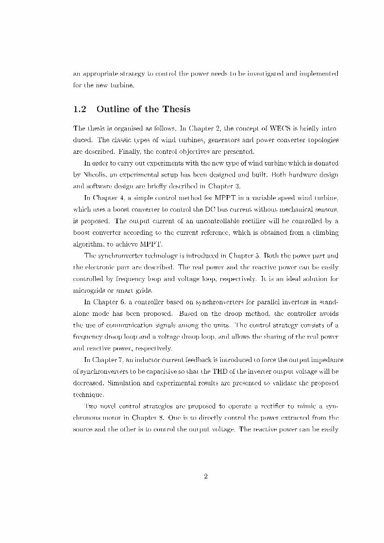
an appropriate strategy to control the power needs to be investigated and implemented
for the new turbine.
1.2 Outline of the Thesis
The thesis is organised as follows. In Chapter 2, the concept of WECS is briey intro-
duced. The classic types of wind turbines, generators and power converter topologies
are described. Finally, the control objectives are presented.
In order to carry out experiments with the new type of wind turbine which is donated
by Nheolis, an experimental setup has been designed and built. Both hardware design
and software design are briey described in Chapter 3.
In Chapter 4, a simple control method for MPPT in a variable speed wind turbine,
which uses a boost converter to control the DC bus current without mechanical sensors,
is proposed. The output current of an uncontrollable rectier will be controlled by a
boost converter according to the current reference, which is obtained from a climbing
algorithm, to achieve MPPT.
The synchronverter technology is introduced in Chapter 5. Both the power part and
the electronic part are described. The real power and the reactive power can be easily
controlled by frequency loop and voltage loop, respectively. It is an ideal solution for
microgrids or smart grids.
In Chapter 6, a controller based on synchronverters for parallel inverters in stand-
alone mode has been proposed. Based on the droop method, the controller avoids
the use of communication signals among the units. The control strategy consists of a
frequency droop loop and a voltage droop loop, and allows the sharing of the real power
and reactive power, respectively.
In Chapter 7, an inductor current feedback is introduced to force the output impedance
of synchronverters to be capacitive so that the THD of the inverter output voltage will be
decreased. Simulation and experimental results are presented to validate the proposed
technique.
Two novel control strategies are proposed to operate a rectier to mimic a syn-
chronous motor in Chapter 8. One is to directly control the power extracted from the
source and the other is to control the output voltage. The reactive power can be easily
2

controlled to obtain the unity power factor. Control schemes are veried through Mat-
lab simulation. It is implemented on a dSPACE-based digital controller and tested on
a prototype.
In Chapter 9, a strategy is proposed to control the output voltage of a three-phase
PWM-controlled rectier, based on the synchronverter technology that operates PWM
converters to mimic synchronous machines. Such a PWM-controlled rectier is able to
track the grid frequency and phase so that an extra synchronisation unit, e.g. a PLL,
is not needed any more, which considerably reduces the computational burden of the
controller.
A control strategy based on the synchronverter technology is proposed for back-
to-back PWM converters in Chapter 10. Both converters are run as synchronverters,
which are mathematically equivalent to the conventional synchronous generators. The
rotor-side converter is responsible for maintaining the DC bus voltage and the grid-side
converter is responsible for MPPT. Simulation results show that the proposed method
operates properly, even in the situation of grid voltage sags.
Finally, the main conclusions of the thesis are summarised and further research is
proposed in Chapter 11.
1.3 Major Contributions
1.3.1 Current control for maximum power point tracking
As is well known, the rotating speed of a generator is proportional to the peak output
voltage with constant excitation, meanwhile the torque of the machine is proportional to
the peak output current with constant excitation. In this control strategy, the current
reference of the input current of the boost converter is determined from the climbing
algorithm according to the speed of the generator. The input current of the boost
converter will be controlled to follow the current reference by PI control. As a result,
the wind turbine can generate the maximum output power in dierent wind speeds.
1.3.2 Rectier control based on synchronverters
Two control strategies are proposed to operate a rectier to mimic a synchronous mo-
tor, following the idea of operating inverters to mimic synchronous generators. The
controllers have two channels: one for the real power and the other for the reactive
3
power. The real power is controlled by a frequency control loop, which is implemented
by comparing the virtual angular speed θwith the grid angular frequency reference θg,
and adding this dierence, multiplied with a gain, to the active mechanical torque Tm.
This loop regulates the virtual angular speed θ of the synchronous motor and creates
the phase angle θ for the control signal e. Meanwhile, the reactive power is regulated
by a voltage control loop. This loop regulates the eld excitation Mf if , which is pro-
portional to the amplitude of the control signal e. As a result, the reactive power can
be easily controlled to be zero in the steady state so that the unity power factor is
obtained. Furthermore, the line currents can be made sinusoidal and good dynamics
can be achieved.
Moreover, improved control strategies that are able to self-synchronise with the
grid are presented. As a result, an extra synchronisation unit, e.g. a PLL, is no
longer needed for three-phase rectiers. Proposed control schemes can automatically
synchronise themselves with the grid before connection and track the grid frequency
after connection. It considerably reduces the computational burden of the controller.
1.3.3 Synchronverter-based control in wind power
Back-to-back converters are the most popular topologies in wind power applications.
Most of the control strategies are mainly based on the vector control approach in the
d-q reference frame to control the direct component and quadrature component, respec-
tively. In this work, an original control strategy based on the synchronverter technology,
which is to operate a converter to mimic a synchronous machine, is proposed for back-
to-back converters in wind power applications. The rotor-side converter is run as a
synchronous motor and the grid-side converter is run as a synchronous generator. As a
consequence, the whole system behaves as a generator-motor-generator system.
1.4 List of Publications
1. Z. Ma. A sensorless control method for maximum power point tracking of wind
turbine generators. In proceedings of the 14th European Conference on Power
Electronics and Applications (EPE2011). Birmingham, September, 2011.
2. Z. Ma, Q.-C. Zhong and J. Yan. Synchronverter-based control strategies for three-
phase PWM rectiers. In proceedings of the 7th IEEE Conference on Industrial
4

Electronics and Applications (ICIEA2012), Singapore, July, 2012.
3. Z. Ma and Q.-C. Zhong. Synchronverter-based control strategy for back-to-back
converters for wind power applications. In proceedings of the 8th Power Plant and
Power System Control Symposium (PPPSC2012), Toulouse, September, 2012.
4. Q.-C. Zhong, Z. Ma and P.-L. Nguyen. PWM -controlled Rectiers without the
Need of an Extra Synchronisation Unit. In proceedings of the 38th Annual Confer-
ence of the IEEE Industrial Electronics Society (IECON2012), Montreal, October,
2012.
5. Q.-C. Zhong, Z. Ma and J. Yan. Synchronverter-based control strategies for three-
phase PWM rectiers. submitted to IEEE Trans on Power Electronics.
6. Q.-C. Zhong and Z.Ma. Synchronverter-based control strategy for back-to-back
converters for wind power applications. submitted to IEEE transactions on Energy
Conversion.
7. Q.-C. Zhong, P.-L. Nguyen and Z. Ma. Self-synchronised Synchronverters, IEEE
Trans on Power Electronics, under review.
8. Q.-C. Zhong, G. Weiss, P.-L. Nguyen and Z. Ma. Synchronverters: Operating
Power Converters as Synchronous Machines. IEEE Transactions on Industrial
Electronics, invited paper.
5

Chapter 2
Wind Energy Conversion Systems
Wind energy has been regarded as an environmentally friendly, logistically feasible and
economically responsible alternative energy resource. Many countries have set strategic
plans to develop technology for utilising wind power and a lot of researchers have shifted
into this area. During the last decade, more and more attention has been paid to
utilising renewable energy sources to tackle the energy crisis we are facing. Wind power
has attracted most of the attention and many countries have launched various initiatives
to increase the share of wind power in electricity generation [2, 3].
Wind energy conversion is a complex process. The blades of a wind turbine rotor
extract some of the ow energy from air in motion, convert it into rotational energy,
then deliver it via a mechanical drive unit (shafts, clutches and gears) to the rotor of
a generator and thence to the stator of the same by mechanical-electrical conversion.
The electrical energy from the generator is fed via a system of switching and protection
devices, leads and any necessary transformers to the mains, to the end user or to some
means of storage or utility power grid. During the past 30 years, wind energy conversion
has become a reliable and competitive means for electric power generation. The life
span of modern wind turbines is now 20-25 years, which is comparable to many other
conventional power generation technologies. The cost of wind power has continued to
decline through technological development, increased production level, and the use of
larger turbines [4].
The major components of a typical wind energy conversion system include a wind
turbine, a generator, interconnection apparatus, and control systems. At the present
time and for the near future, generators for wind turbines will be synchronous gener-
ators, permanent magnet synchronous generators, and induction generators, including
6

the squirrel-cage type and wound rotor type. For small to medium power wind tur-
bines, permanent magnet generators and squirrel-cage induction generators are often
used because of their reliability and cost advantages. Induction generators, permanent
magnet synchronous generators, and wound eld synchronous generators are currently
used in various high power wind turbines.
Interconnection apparatuses are devices to achieve power control, soft start, and
interconnection functions. Very often, power electronic converters are used as such de-
vices. Most modern turbine inverters are forced commutated PWM inverters which
provide a xed voltage and xed frequency output with a high power quality. Both
voltage source voltage controlled inverters and voltage source current controlled invert-
ers have been applied in wind turbines. For certain high power wind turbines, the
eective power control can be achieved with double PWM converters, which provide a
bidirectional power ow between the turbine generator and the utility grid.
2.1 Wind Turbines
A wind turbine is a device that captures the kinetic energy of wind. Historically, a wind
turbine was frequently used as a mechanical device with a number of blades to drive
machinery. Nowadays, it is often used to drive a generator so that the kinetic energy
is converted to electricity. The main types of wind turbines are shown in Figure 2.1
[5]. Most modern wind turbines use a horizontal axis conguration with two or three
blades, operating either downwind or upwind [6]. The typical structure of a horizontal
axis wind turbine is shown in Fig 2.2. The major components include blades, a rotor
hub, drivetrain (bearing and gears etc), a generator and the associated control system.
Wind turbines can be used for stand-alone applications, or they can be connected
to a utility power grid, or even combined with a photovoltaic system, batteries, and
diesel generators, called hybrid systems. Stand-alone turbines are typically used for
water pumping or communications. However, homeowners and farmers in windy areas
can also use turbines to generate electricity. For utility-scale sources of wind energy, a
large number of turbines are usually built close together to form a wind farm.
Assume that the wind speed is vw m/s and the area swept by a wind turbine is A
m2. Then the volume of air swept through in unit time is Avw. If the density of air is ρ
kg/m3, then the mass of air m passing through the area in unit time is ρAvw kg. The
7

Figure 2.1: Main turbine types. (Grid integration of wind energy conversion systems(second edition), Fig.2.12 Main turbine types, pp.47')
kinetic energy of this mass of air moving at velocity vw in unit time is
1
2mv2
w =1
2ρAv3
w.
This is actually the same as the power carried by the wind motion. For a wind turbine
with rotor blades of R m long, the area swept is A = πR2 and hence the wind power
available is
Pw =1
2ρπR2v3
w.
In reality, it is impossible to convert all the energy into electricity. The actual power
produced by a wind turbine can be calculated as
Pm = 0.5πρCp(λ, β)R2v3ω, (2.1)
where Cp(λ, β) is the power coeecient dependent on the turbine design, the pitch angle
β and the tip-speed ratio λ dened as
λ = ωrR/vω, (2.2)
where ωr is the angular speed of the wind turbine. The tip-speed ratio plays a vital role
in extracting power from wind. If the rotor turns too slowly, most of the wind passes
through the gap between the rotor blades without doing any work; if the rotor turns too
quickly, the blurring blades blocks the wind like a solid wall. Therefore, wind turbines
are designed to run at optimal tip-speed ratios so that as much power as possible can
be extracted from the wind.
8

Figure 2.2: Diagram of a typical wind turbine. (Grid integration of wind energy con-version systems (second edition), Figure 2.50 Hydraulic blade pitch-regulation systemwith positioning cylinder and lever transmission (WKA 60, MAN) pp.85')
In Equation 2.1, Cp is a highly nonlinear power function of λ and β. Normally, the
pitch has a xed angular position on the hub of the wind turbine. As a result, the pitch
angle is constant. With a xed β, the relationship between power eciency Cp and
the tip speed ratio λ can be depicted as shown in Figure 2.3(a). At the point λopt, the
power eciency will reach its maximum point. Moreover, based on Equation 2.2, the
curves of Cp against various wind speeds should have similar shapes but vary in specic
values as indicated in Figure 2.3(b), in which six curves of Cp are shown according to
dierent wind speeds vω1, vω2, vω3, vω4, vω5, and vω6. Therefore, the operation points
of the wind turbine for various wind speeds are dierent, which are determined by the
point λopt, see more details in [5]. It is worth noting that the power coecient Cp of a
wind turbine is limited by 1627 ≈ 0.593, according to the Betz law1.
A wind turbine can be designed for a xed-speed or variable-speed operation. Variable-
speed wind turbines can produce 8% to 15% more energy output as compared to their
xed-speed counterparts; however, they necessitate power electronic converters to pro-
vide a xed frequency and xed voltage power to their loads. Most turbine manufac-
turers have opted for reduction gears between the low speed turbine rotor and the high1http://en.wikipedia.org/wiki/Betz%27_law
9

Po
wer
eff
icie
ncy
Cp
Tip speed ratio λλ
opt
(a) Cp as a function of tip speed ratio λ.
00
0.1
0.2
0.3
0.4
0.5
Pow
er e
ffic
ienc
y C
p
Turbine speed (pu)0.2 0.4 0.6 0.8 1 1.2 1.4 1.6
vω6
vω5
vω4
vω3
vω2
vω1
(b) Cp as a function of turbine speed for various wind speeds.
Figure 2.3: Power coeciency Cp curves.
speed three-phase generators. Direct drive conguration, where a generator is coupled
to the rotor of a wind turbine directly, oers high reliability, low maintenance, and
possibly low cost for certain turbines.
2.2 Generators
In electricity generation, an electric generator is a device that converts mechanical
energy to electrical energy. A generator forces electric charge to ow through an external
electrical circuit. The xed-speed wind turbines were mostly manufactured with a
squirrel-cage induction generator (SCIG) and a multiple-stage gearbox during the 1980's
and 1990's. Since the late 1990's, most wind turbines, whose power level was increased
above 1.5MW, have been changed to the variable-speed control because of the grid
requirement for good power quality. Generator systems of variable speed wind turbines
10

mostly consist of a doubly-fed induction generator (DFIG), a multiple-stage gearbox and
a power electronic converter. Since 1991, permanent magnet synchronous generators
(PMSG) have been built to reduce failures in the gearbox and to lower maintenance
problems [7].
2.2.1 Squirrel-cage induction generators
An SCIG is a device that converts the mechanical energy of rotation into electricity
based on electromagnetic induction. An electric voltage (electromotive force) is induced
in a conducting loop (or coil) when there is a change in the number of magnetic eld lines
(or magnetic ux) passing through the loop. When the loop is closed by connecting the
ends through an external load, the induced voltage will cause an electric current to ow
through the loop and load. Thus rotational energy is converted into electrical energy.
In general, the pole pair number is mostly equal to 2 or 3 in this type of commercial
xed-speed wind turbine with SCIG, so that the synchronous speed in a 50Hz-grid is
equal to 1000 or 1500rpm. Therefore, a three-stage gearbox in the drive train is usually
required[7].
The advantages of SCIG are well-known and it is a robust technology; it is easy and
relatively cheap mass production of the generator. In addition, there is no electrical
connection between stator and rotor system. Furthermore, it enables stall regulated
machines to operate at a xed speed when it is connected to a large grid which provides
a stable control frequency, which is the most common type of generator used for the
grid connected wind turbines.
However, the SCIG has its own disadvantages. First of all, the speed is not control-
lable, and is variable only over a very narrow range. Secondly, a three-stage gearbox in
the drive train is necessary. Gearboxes represent a large mass in the nacelle, and also
a large fraction of the investment costs. They are relatively maintenance intensive and
a possible source of failures. Moreover, it is necessary to obtain the excitation current
from the stator terminals. This makes it impossible to support grid voltage control[4].
2.2.2 Doubly fed induction generators
The fact that the rotor circuit of a SCIG is not accessible can be changed if the ro-
tor circuit is wound and made accessible via slip rings, which oers the possibility of
controlling the rotor circuit so that the operational speed range of the generator can
11

be increased in a controlled manner. The rotor circuit is often connected to back-to-
back power electronic converters, which consists of a rotor-side converter and a grid-side
converter sharing the same DC bus, so that the dierence between the mechanical fre-
quency and the electrical frequency can be compensated via injecting a current with a
variable frequency into the rotor circuit. Hence, the operation during both normal and
faulty conditions can be regulated via controlling the converters.
A DFIG can be excited by the rotor windings and does not have to be excited by
the stator windings. If needed, the reactive power needed for the excitation from the
stator windings can be generated by the grid-side converter. As a result, a wind power
plant equipped with DFIGs can easily take part in the regulation of voltage. The stator
always feeds real power to the grid but the real power in the rotor circuit can ow
bidirectionally, from the grid to the rotor or from the rotor to the grid, depending on
the operational condition. Ignoring the losses, the power handled by the rotor circuit is
[8]
Protor = −s · Pstator
and the power sent to the grid is
Pgrid = Protor + Pstator = (1− s)Pstator,
where s is the slip. Since most of the power ows through the stator circuit, the power
processed by the rotor circuit can be reduced to roughly 30%. This means that the great
advantage of a sucient range of operational speed can be achieved with a reasonably
low cost[9].
2.2.3 Permanent magnet synchronous generators
A PMSG adopts a permanent magnet to generate the magnetic eld needed for elec-
tricity generation and hence there is no need to provide an external power supply for
excitation or to have a rotor circuit. This simplies the structure and reduces the main-
tenance cost. PMSGs are more ecient than inductor generators and the power factor
can be unity or even leading. Moreover, PMSGs have very high power density and the
price of rare-earth magnets has reduced by more than an order of magnitude in the
last 10 years. As a result, PMSGs are becoming increasingly popular for wind power
applications. A PMSG runs at the synchronous speed, and the frequency of electricity
generated is directly in proportion to the mechanical speed, and hence the slip is zero.
12

This could be used to eliminate the need for a mechanical sensor to measure the speed of
the turbine. Compared to the DFIG this generator system has the following advantages
[7]:
1. higher eciency and energy yield,
2. no additional power supply for the magnet eld excitation,
3. higher reliability due to the absence of mechanical components such as slip rings,
4. improvement in the thermal characteristics of the machine due to the absence of
the eld losses.
However, PMSG has disadvantages and these can be summarised as follows:
1. high cost,
2. diculty to handle in manufacture,
3. demagnetisation of PM at high temperature.
2.3 Power Converter Topologies
Various wind turbine topologies have been developed and built to maximise energy
capture, minimise costs, provide consistent dynamic response, improve power quality,
and ensure safety together with the growth of wind energy during last two decades.
The three main types of topologies for wind turbines are as detailed below [10].
The rst type is a xed-speed wind turbine system using a multi-stage gearbox and
a standard squirrel-cage induction generator, directly connected to the grid through a
transformer as shown in Fig 2.4(a). The rotor blades have a simple construction because
the blade is directly xed on the hub. The rotor blades of this type are adjusted only
once when the turbine is erected. The power limitation over the rated wind speed is
achieved bu the stall eect of the rotor blades. The wind turbine with this topology
is completely passive while the wind causes the power regulation by itself. Therefore,
this topology is called a passive stall control, or briey a stall control. In most cases,
capacitors are grid-connected parallel to the generator to compensate for the reactive
power consumption.
13

The second type is a variable speed wind turbine system with a multi-stage gearbox
and a doubly fed induction generator. The power electronic converter feeding the rotor
winding has a power rating of approximately 30% of the rated power; the stator winding
of the DFIG is directly connected to the grid as shown in Fig 2.4(b). The stator is
constructed in the same way with a SCIG. The rotor is equipped with a three-phase
winding and connected to the grid through the power electronic converter. The basic
operation principle is the same as a SCIG. However, the rotor active power can be
controlled by the current of the rotor side converter. Typically, by controlling the rotor
active power ow direction, a speed range ±30% around the synchronous speed can
be obtained. Instead of dissipating the rotor energy, it can be fed into the grid. The
choice for the rated power of the rotor converter is a trade-o between costs and the
speed range desired. Moreover, this converter performs reactive power compensation
and smooth grid connection.
The third type is also a variable speed wind turbine, but it is a gearless wind tur-
bine system with a permanent magnet synchronous generator. It uses a low-speed
high-torque synchronous generator and an AC-DC-AC electronic converter for the grid
connection as shown in Fig 2.4(c). A full-scale back-to-back converter can be used as
AC-DC-AC converter. Another popular AC-DC-AC converter includes an uncontrol-
lable rectier, a DC-DC converter and an inverter.
2.4 Control Objectives
The need for control goes back to the origins of wind turbines. Wind turbines are
complex, nonlinear, dynamic systems forced by gravity, stochastic wind disturbances,
and gravitational, centrifugal, and gyroscopic loads. The aerodynamic behaviour of
wind turbines is nonlinear, unsteady and complex. Designs of control algorithms for
wind turbines must account for these complexities. The control strategies of the wind
turbine can be classied into four categories, namely [4]:
1. Fixed-speed xed-pitch: FS-FP is very simple and low-cost. But its performance is
rather poor. In fact, no active control action can be done to alleviate mechanical
loads and improve power quality. Further, the conversion eciency is far from
optimal.
14

Transformer
Grid
SCIG Gearbox
Capacitor
(a) SCIG topology.
Transformer
Grid
DFIG Gearbox
AC-DC-AC Converter
(b) DFIG topology.
Transformer
Grid
PMSG
AC-DC-AC Converter
(c) PMSG topology.
Figure 2.4: Power converter topologies.
2. Fixed-speed variable-pitch: This type can improve the power quality and the
conversion eciency in high wind speeds. The variable-pitch operation enables
an ecient power regulation at higher than rated wind speeds.
3. Variable-speed xed-pitch: This type can improve the power quality and the
conversion eciency in low wind speeds. The variable-speed operation increases
the energy capture at low wind speeds.
4. Variable-speed variable-pitch: This control strategy is the best method for the
wind turbine system, but it is also the most complicated one. It can improve the
power quality and the conversion eciency in any wind speed.
The main control goals were the limitation of power and speed below some specied
values to prevent the turbine from unsafe operation under high wind conditions. Former
15

wind turbines included primitive mechanical devices to attain these objectives. As wind
turbines augmented in size and power, control specications became more demanding
and regulation mechanisms more sophisticated. Increasingly, control systems have been
expected not merely to keep the turbine within its safe operating region but also to
improve eciency and quality of power conversion. They gradually evolved as a con-
sequence until playing today a decisive role in modern turbines. These goals can be
arranged in the following topics: energy captures, mechanical loads and power quality
[11].
2.4.1 Energy capture
For a wind turbine, the generation capacity species how much power can be extracted
from the wind, taking into consideration both physical and economic constraints. Nor-
mally, wind generation systems can be divided into variable-speed generation systems
and xed-speed generation systems. Variable-speed generation systems are more attrac-
tive compared to xed-speed ones. This is because the power eciency Cp in variable-
speed generation systems can be controlled to reach its maximum value and hence the
mechanical power of a variable-speed wind turbine is commonly higher than that of a
similar xed-speed wind turbine for various wind speeds [5].
The target maximum power point of a wind turbine system can be written as
Pmax = Koptωropt,
where
Kopt =0.5πρCpmaxR
5
λ3opt
,
wopt =λoptvωR
.
Hence, the maximum mechanical power for a certain wind speed can be obtained at
a certain wind turbine speed known as the optimum wind turbine speed ωopt, which
corresponds to a certain optimum tip speed ratio λopt. In order to extract the maxi-
mum power from the wind energy, the turbine should always be operated at λopt via
controlling the turbine speed.
Figure 2.5 shows the turbine mechanical power against turbine speed for various
wind speeds. An advanced technique should be applied to extract the maximum power
from the wind turbine under all working conditions as indicated in Figure 2.5. Basically,
16

0 0
0.20.40.60.8
11.21.41.6
Mec
hani
cal P
ower
(pu
)
Turbine speed (pu)0.2 0.4 0.6 0.8 1 1.2 1.4 1.6
vω1
vω2
vω3vω4vω5vω6
Figure 2.5: Mechanical power curves of turbine speed for various wind speeds.
the MPPT controllers can be classied into three types, e.g. TSR control, PSF control
and HCS control. For TSR control, with the knowledge of the relationship between the
tip speed ratio and the extracted power, both the wind speed and the turbine speed are
measured or estimated to maintain the TSR at an optimum value and then extract the
maximum possible power. In PSF control, the power is measured as a feedback to be
controlled to reach the turbine's maximum power point. As a result, the power curve
of the wind turbine is needed, which can be obtained through simulation or o-line
experiments. Dierent from the previous two methods, in HCS control, the maximum
power point is continuously searched depending on the current operating power point
and the relationship between the changes in power and speed.
2.4.2 Mechanical loads
Keeping in mind the minimisation of the energy cost, the control system should not
be merely designed to track as tightly as possible the ideal power curve. In fact, the
other control objectives should not be ignored. For instance, the mechanical loads that
wind turbines are exposed to must be considered. Mechanical loads may cause fatigue
damage on several devices, thereby reducing the useful life of the system.
There are basically two types of mechanical loads, namely static and dynamic ones
[12]. Static loads result from the interaction of the turbine with the mean wind speed.
Much more important from the control viewpoint are the dynamic loads, which are
induced by the spatial and temporal distribution of the wind speed eld over the area
swept by the rotor. Dynamic loads comprise variations in the net aerodynamic torque
17

that propagate down the drive-train, and variations in the aerodynamic loads that
impact on the mechanical structure [5].
2.4.3 Power quality
Power quality aects the cost of energy in several ways. For instance, poor power
quality may demand additional investments in power lines, or may impose limits to the
power supplied to the grid. Because of the long-term and short-term variability of the
energy resource and the interaction with the power network, wind generation facilities
are conventionally considered as poor quality suppliers. Therefore, the control system
design must also take power conditioning into account. This control requirement in
more and more relevant as the power scale of wind generation facilities approaches the
output rating of conventional power plants. Power quality is mainly assessed by the
stability of the frequency and voltage at the point of connection to the grid and by the
emission of icker.
18

Chapter 3
Experimental Setup
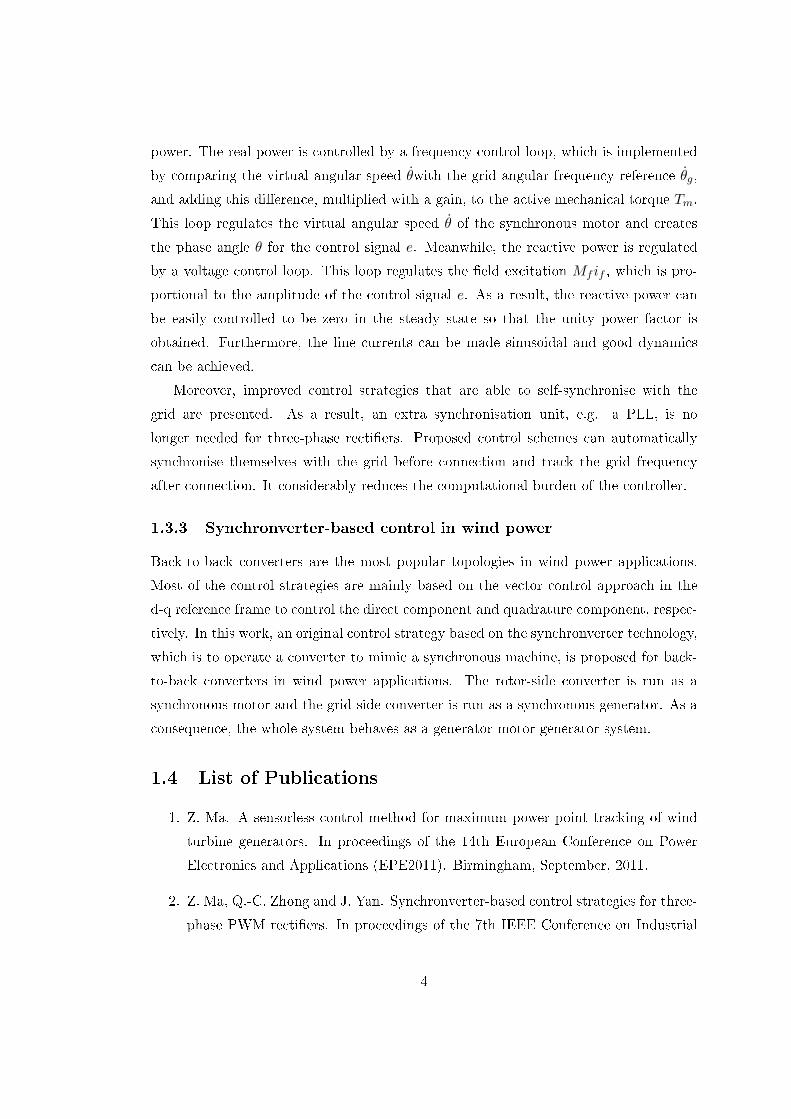
In order to carry out real-time experiments with the wind turbine in Figure 3.1, which
was donated by Nheolis SAS corporation, an experimental setup has been designed and
built. It mainly consists of a power-processing device (including a rectier, maximum
power tracking system, an energy storage system and an inverter) and a braking system
to safeguard the operation of the wind turbine. All these are controlled by a central
controller eZdspF28335, which is from Texas Instruments. From this gure, the wind
turbine has been installed on the roof of the department's building. All components
should be placed in a control panel. A remote MMI is placed remotely to monitor the
operation of the wind turbine, via communication. The supervisor computer has been
set up in the G05 Lab. All components have been designed and made by the PHD
researcher except a Semistack IGBT device which purchased from Semikron. In this
chapter, the experimental system design and development are briey described.
3.1 Hardware Design
3.1.1 Power circuits
The topology of the main circuits is shown in Figure 3.2. For the wide range of variable
speed operation, a DC-DC boost chopper is utilised between a 3-phase diode rectier
and the IGBT inverter.
3.1.1.1 Semistack IGBT
The Semistack IGBT device, which is from Semikron, consists of a three-phase uncon-
trolled rectier, some components on the DC bus and a three-phase inverter. The device
19
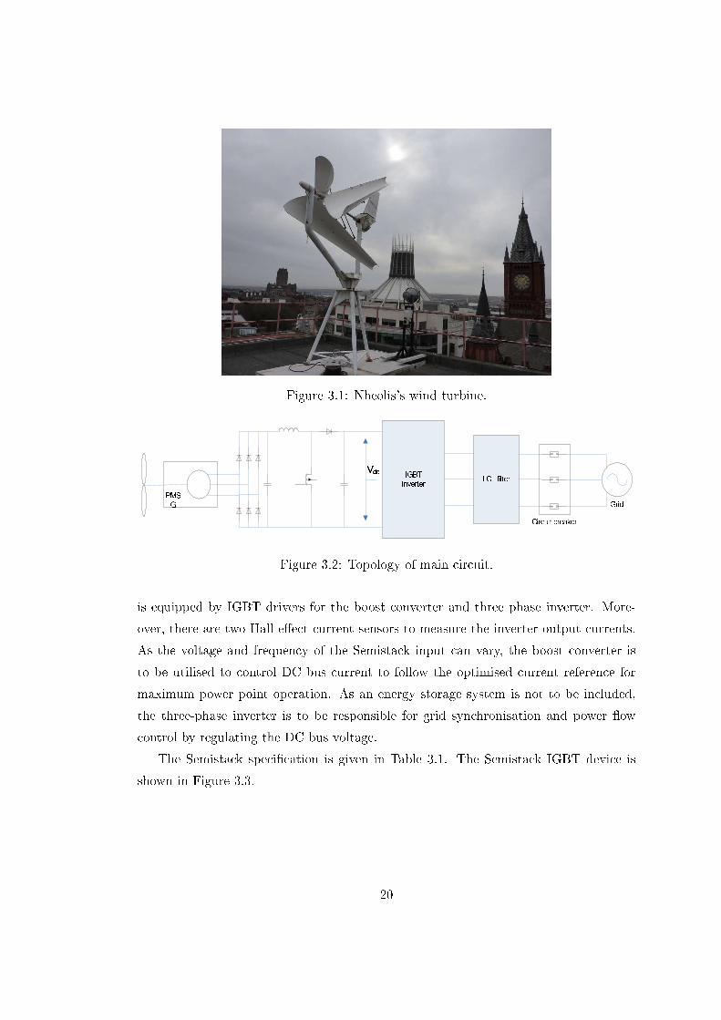
Figure 3.1: Nheolis's wind turbine.
PMSG IGBTInverterVdc LCL filter Circuit breaker Grid Figure 3.2: Topology of main circuit.
is equipped by IGBT drivers for the boost converter and three phase inverter. More-
over, there are two Hall-eect current sensors to measure the inverter output currents.
As the voltage and frequency of the Semistack input can vary, the boost converter is
to be utilised to control DC bus current to follow the optimised current reference for
maximum power point operation. As an energy storage system is not to be included,
the three-phase inverter is to be responsible for grid synchronisation and power ow
control by regulating the DC bus voltage.
The Semistack specication is given in Table 3.1. The Semistack IGBT device is
shown in Figure 3.3.
20
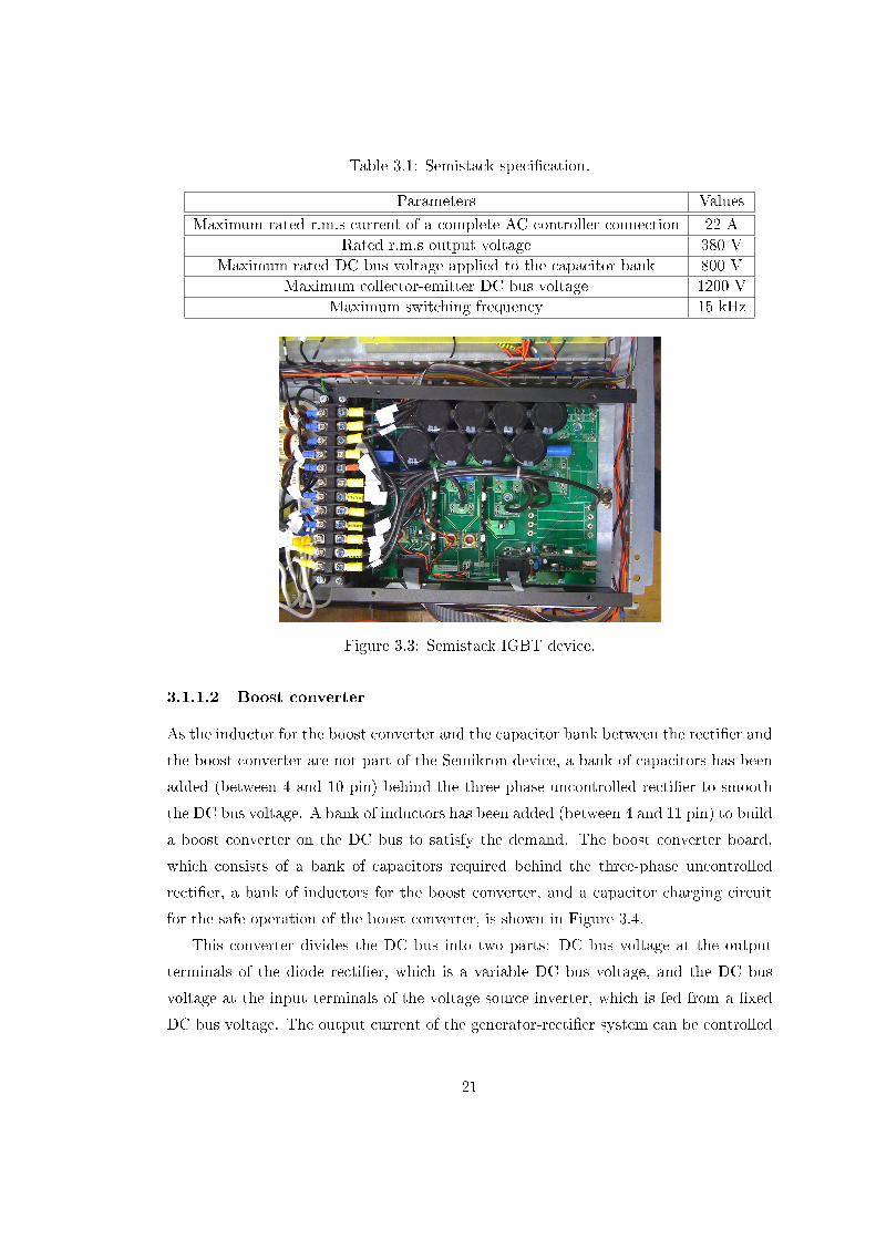
Table 3.1: Semistack specication.
Parameters ValuesMaximum rated r.m.s current of a complete AC controller connection 22 A
Rated r.m.s output voltage 380 VMaximum rated DC bus voltage applied to the capacitor bank 800 V
Maximum collector-emitter DC bus voltage 1200 VMaximum switching frequency 15 kHz
Figure 3.3: Semistack IGBT device.
3.1.1.2 Boost converter
As the inductor for the boost converter and the capacitor bank between the rectier and
the boost converter are not part of the Semikron device, a bank of capacitors has been
added (between 4 and 10 pin) behind the three-phase uncontrolled rectier to smooth
the DC bus voltage. A bank of inductors has been added (between 4 and 11 pin) to build
a boost converter on the DC bus to satisfy the demand. The boost converter board,
which consists of a bank of capacitors required behind the three-phase uncontrolled
rectier, a bank of inductors for the boost converter, and a capacitor charging circuit
for the safe operation of the boost converter, is shown in Figure 3.4.
This converter divides the DC bus into two parts: DC bus voltage at the output
terminals of the diode rectier, which is a variable DC bus voltage, and the DC bus
voltage at the input terminals of the voltage source inverter, which is fed from a xed
DC bus voltage. The output current of the generator-rectier system can be controlled
21

Figure 3.4: Boost converter board.
by changing the duty cycle of the switch. Its purpose is to control the rectier output
current so that the maximum power can be captured from the wind by the turbine.
3.1.1.3 LCL lter
The high-frequency switching of a PWM converter may produce harmonics and inter-
harmonics, which are in the range of some kilohertz. Due to the high frequency, the
harmonics are relatively easy to remove by small-size lters. The lter board designed
for the output of the inverter connects to pins 7,8 and 9. The LCL lter is connected
in parallel as an interface between the inverter and the utility grid. The LCL lter
board is equipped with a variety of measuring terminals to provide more freedom for
control algorithm with dierent current feedback to be measured. This will allows, if
necessary, multiloop control to be implemented, ensuring steady-state reference tracking
performance and fast dynamic compensation for system disturbances (including sudden
reference or load changes) and improving stability. The LCL lter board is shown in
Figure 3.5.
3.1.2 Control circuits
Control circuits include the measurement transducers board and the I/O conditioning
board.
22

Figure 3.5: LCL lter.
3.1.2.1 Measurement transducers board
The measurement transducers board, as shown in Figure 3.6, consists of 2 current (LA
25-NP) LEM transducers and 10 voltage (LV 25-P) LEM transducers with instanta-
neous current and voltage output respectively. The PCB layout of the measurement
transducers board is given in Appendix A.
For the voltage transducers, the selection of the primary resistor is very important
for the circuit design. As we know, the transducer's optimum accuracy is obtained at
the nominal primary current. As far as possible, the primary resistor R1 (see Appendix
A) should be calculated so that the nominal voltage to be measured corresponds to a
primary current of 10mA.
For example, the measurement range of grid voltage of each phase is 325V. The pri-
mary nominal current is 10mA. The primary resistor R1 should be calculated in Equa-
tion 3.1. Moreover, the heat dissipation issues should be taken into account. Therefore,
three 100W resistors in parallel have been used for these reasons.
R1 =VgridIpn
=325
0.01= 32.5KΩ (3.1)
23

Figure 3.6: Measurement transducers board.
3.1.2.2 Control board
F28335 digital signal controllers include multiple complex peripherals running at fairly
high-clock frequencies. They are commonly connected to low-level analog signals using
an onboard analog-to-digital converter. The control board has been designed to be
employed like an interface between the power circuits and the TI DSP. The digital
signal controller TMS320F28335 is a 32-bit oating-point digital signal controller DSP
and is xed on the top of the control board, as shown in Figure 3.7. The operating speed
is 150 MHz (30 MHz input clock). The integrated peripherals of the TMS320F28335
device used in this project are shown as follows: 12 input channels with a 12-bit Analog
to Digital Converter (ADC), 7 enhanced PWM modules (ePWM) and 4 digital general
purpose I/O (GPIO). Table 3.2, 3.3 and 3.4 show the list of ADC, ePWM and GPIO
channels.
The ADC module consists of a 12-bit ADC with a built-in sample-and-hold (S/H)
circuit and provides a exible interface to peripherals with a fast conversion rate of up
to 80 ns at 25 MHz ADC clock. The ADC module has 16 channels, congurable as two
independent 8-channel modules.
The ePWM peripheral performs a digital to analog (DAC) function, where the
duty cycle is equivalent to a DAC analog value. The ePWM module represents one
24

Table 3.2: ADC list.
ADC (Analog Inputs)No. Variable name Voltage level Range Transducer1 Gen.voltage phase A ±3Vdc 230Vac LV 25-P2 Gen.voltage phase B ±3Vdc 230Vac LV 25-P3 Gen.voltage phase C ±3Vdc 230Vac LV 25-P4 Gen.current phase A ±3Vdc 10A LA 25-NP5 Gen.current phase B ±3Vdc 10A LA 25-NP6 Gen.current phase C ±3Vdc 10A LA 25-NP7 Grid.voltage phase A ±3Vdc 230Vac LV 25-P8 Grid.voltage phase B ±3Vdc 230Vac LV 25-P9 Grid.voltage phase C ±3Vdc 230Vac LV 25-P10 Idc ±3Vdc 10A LA 25-NP11 Vdc ±3Vdc 800Vdc LV 25-P12 Vin ±3Vdc 400Vdc LV 25-P
Table 3.3: ePWM list
ePWMNo. Variable name Voltage level Frequency1 Inverter leg Wtop switch 0/15V 10kHz2 Inverter leg Wbotton switch 0/15V 10kHz3 Inverter leg Utop switch 0/15V 10kHz4 Inverter leg Ubotton switch 0/15V 10kHz5 Inverter leg Vtop switch 0/15V 10kHz6 Inverter leg Vbotton switch 0/15V 10kHz7 Boost converter 0/15V 10kHz
Table 3.4: GPIO list
GPIONo. Variable name Voltage level I/O signal1 Three phase circuit breaker 0/15V Input contact2 Three phase circuit breaker 0/24V Output relay3 Charging relay (Boost converter) 0/15V Input contact4 Charging relay (Boost converter) 0/24V Output relay
25

7
For example, the measurement range of grid voltage of each phase is 325V. The primary
nominal current is 10mA. The primary resistor R1 should be calculated as follow 1 32532.5
0.01
gridpnVR k
I
Not only that, the heat dissipation issues should be taken into account. So three 100 k
power resistors in parallel have been used for these reasons.
2.2.2 I/O conditioning board
F28335 digital signal controllers include multiple complex peripherals running at fairly high-
clock frequencies. They are commonly connected to low-level analog signals using an
onboard analog-to-digital converter. The I/O conditioning board has been designed is
employed like an interface between power circuits and TI DSP. As the TI DSP controller uses
3.3V voltage level signals, the ADC inputs must be adjusted from +/-15V and PWM, DI and
DO signals must be processed via optocouplers with 3.3V on the controller side and 15V on
the opposite (15V CMOS signal are necessary to control Semikron device).
Fig. 9 I/O conditioning board
Specific schematics of ADC, DI, DO and PWM are shown as follows.
Digital Input Digital Output ADC PWM
Figure 3.7: Control board.
complete PWM channel composed of two PWM outputs. The ePWM modules are
chained together via a clock synchronisation scheme that allows them to operate as
a single system when required. In the case of the three-phase inverter, six switching
elements can be controlled using three ePWM modules, one for each leg of the inverter.
Each leg must switch at the same frequency and all legs must be synchronised.
The GPIO multiplexing (MUX) registers are used to select the operation of shared
pins. These pins can be individually selected to operate as digital I/O, referred to as
GPIO, or connected to one of up to three peripheral I/O signals. If selected for digital
I/O mode, registers are provided to congure the direction of the pin as either input or
output.
The control board, which is shown in Figure 3.7, is employed like an interface be-
tween the power circuits and the TI DSP. As the TI DSP controller uses 3.3V voltage
level signals, the ADC inputs must be adjusted from +/-15V and PWM, DI and DO
signals must be processed via optocouplers with 3.3V on the controller side and 15V
on the opposite (15V CMOS signal are necessary to control the Semikron device). The
26
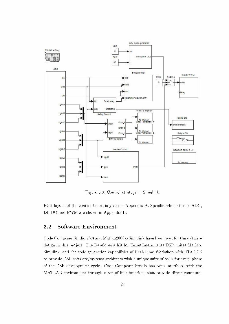
Figure 3.8: Control strategy in Simulink.
PCB layout of the control board is given in Appendix A. Specic schematics of ADC,
DI, DO and PWM are shown in Appendix B.
3.2 Software Environment
Code Composer Studio v3.3 and Matlab2008a/Simulink have been used for the software
design in this project. The Developer's Kit for Texas Instruments DSP unites Matlab,
Simulink, and the code generation capabilities of Real-Time Workshop with TI's CCS
to provide DSP software/systems architects with a unique suite of tools for every phase
of the DSP development cycle. Code Composer Studio has been interfaced with the
MATLAB environment through a set of link functions that provide direct communi-
27

cation between the two applications. The control strategy model has been built in
Simulink (see Figure 3.8). The code will be generated automatically in CCS to debug
the program.
3.2.1 Matlab/Simulink
Matlab is a powerful and well-known tool for engineers and scientists. The Simulink,
integrated with Matlab, is an environment for simulation and model-based design for
dynamic and embedded systems. It provides an interactive graphical environment and
a set of block libraries that allow design, simulation, implementation, and the ability
to test a variety of time-varying systems, including apart from other digital signal
processing and controls.
For TMS320F28335 programming, Target Support Package TC2 for Matlab is used.
The TC 2 package integrates Matlab and Simulink with TI's eXpressDSP tools (Code
Composer Studio). By using the TC2 package, a C-language real-time implementation
of the Simulink model is generated and automatically compiled, and then the generated
code is downloaded to DSP RAM or ash. Onboard DSP peripherals are directly
supported. The Blackhawk USB560 JTAG emulator is used to communicate with the
TI DSP.
3.2.2 Code composer studio
Code Composer Studio is the integrated development environment for TI's DSPs, micro-
controller and application processors. CCS includes a suite of tools used to develop and
debug embedded applications. It includes compilers for each of the TI's device families,
a source code editor, a project build environment, a debugger, a proler, simulators and
many other features. Figure 3.9 shows the CCS's work space.
3.2.3 Communication between host and target
The graphical user interface for this project is designed in Matlab software. For the
development of this GUI, it was necessary to build RTDX to understand the communi-
cation between the controller board and Matlab. This GUI is designed in order to keep
a few things in mind, so that the user is able to diagnose and analyse the performance
of the system by changing the controller parameters such as the type of controller or
28
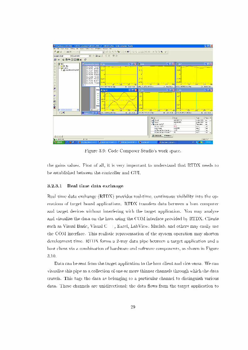
Figure 3.9: Code Composer Studio's work space.
the gains values. First of all, it is very important to understand that RTDX needs to
be established between the controller and GUI.
3.2.3.1 Real time data exchange
Real time data exchange (RTDX) provides real-time, continuous visibility into the op-
erations of target board applications. RTDX transfers data between a host computer
and target devices without interfering with the target application. You may analyse
and visualise the data on the host using the COM interface provided by RTDX. Clients
such as Visual Basic, Visual C++, Excel, LabView, Matlab, and others may easily use
the COM interface. This realistic representation of the system operation may shorten
development time. RTDX forms a 2-way data pipe between a target application and a
host client via a combination of hardware and software components, as shown in Figure
3.10.
Data can be sent from the target application to the host client and vice versa. We can
visualise this pipe as a collection of one or more thinner channels through which the data
travels. This tags the data as belonging to a particular channel to distinguish various
data. These channels are unidirectional; the data ows from the target application to
29

Figure 3.10: RTDX diagram.
Figure 3.11: The eZdsp F28335 and the XDS560 emulator.
the host client and vice-versa. Data can be input into a channel asynchronously at any
time.
The target application sends data to the host by calling functions in the RTDX Tar-
get Library. These functions immediately buer the data and then return. The RTDX
Target Library then transmits the buered data to the host without interfering in the
target application. The host records the data into either a memory buer or an RTDX
log le, depending on the specied RTDX host-recording mode. The recorded data
can be retrieved by any client host application of the RTDX host interface. Windows
platform computers provide a COM interface for the RTDX host interface.
Similarly, a host client can send data to the target. The RTDX Host Library buers
30
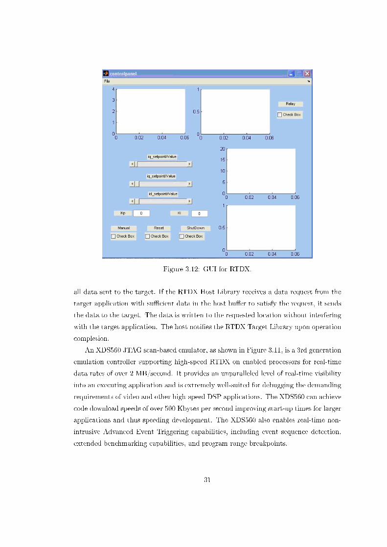
Figure 3.12: GUI for RTDX.
all data sent to the target. If the RTDX Host Library receives a data request from the
target application with sucient data in the host buer to satisfy the request, it sends
the data to the target. The data is written to the requested location without interfering
with the target application. The host noties the RTDX Target Library upon operation
completion.
An XDS560 JTAG scan-based emulator, as shown in Figure 3.11, is a 3rd generation
emulation controller supporting high-speed RTDX on enabled processors for real-time
data rates of over 2 MB/second. It provides an unparalleled level of real-time visibility
into an executing application and is extremely well-suited for debugging the demanding
requirements of video and other high-speed DSP applications. The XDS560 can achieve
code download speeds of over 500 Kbytes per second improving start-up times for larger
applications and thus speeding development. The XDS560 also enables real-time non-
intrusive Advanced Event Triggering capabilities, including event sequence detection,
extended benchmarking capabilities, and program range breakpoints.
31

3.2.3.2 Matlab GUI program
A graphical user interface (GUI) is a graphical display that contains devices, or compo-
nents, that enable a user to perform interactive tasks. To perform these tasks, the user
of the GUI does not have to create a script or type commands at the command line.
Often, the user does not have to know the details of the task at hand.
The GUI components can be menus, toolbars, push buttons, radio buttons, list
boxes, and slidersjust to name a few. In Matlab, a GUI can also display data in
tabular form or as plots, and can group related components.
In order to test the peripheral auxiliary circuit of F28335 and the RTDX, some
communication programs have been made in Matlab by using the graphical user inter-
face. These programs have been developed for the testing of ADC, digital input, digital
output and PWM, respectively. The interface of the control panel is shown in Figure
3.12 and the partial codes are clearly set out in Appendix C.
32

Chapter 4
Maximum Power Point Tracking
Wind power has been regarded as one of the main alternative renewable power sources
to fossil fuels. Many countries have set strategic plans to develop technology for utilising
wind power and a lot of researchers have shifted into this area. During the last decade,
more and more attention has been paid to utilising renewable energy sources to tackle
the energy crisis we are facing. Wind power has attracted most of the attention and
many countries have launched various initiatives to increase the share of wind power in
electricity generation.
Normally, wind generation systems can be divided into variable-speed generation
systems and xed-speed generation systems. Variable-speed generation systems are
more attractive than xed-speed systems due to improved wind energy production and
reduction of the icker problem. The eciency of the wind turbine is higher than
conventional ones. However, it does not mean that the actual eciency is always high.
It depends on the control algorithm used to extract the output power from the wind
turbine. An advanced technique will be designed to extract the maximum power from
the wind turbine under all working conditions. In variable-speed generation systems,
the wind turbine can be operated at its maximum power operating point for various
wind speeds by maintaining the tip speed ratio at the value that maximises aerodynamic
eciency. In order to achieve this ratio, the permanent magnet synchronous generator
load line should be matched very closely to the maximum power line of the wind turbine
generator. A variety of control schemes have been studied in order to produce as much
power as possible from various wind speeds.
During the last few decades, many dierent maximum power point tracking control
strategies have been developed. Among the MPPT methods, the hill-climbing method
33

L Grid C1 C2
PMSG
3-Phase Inverter
LCL Filter
Figure 4.1: Topology of the system.
for comparing kW variation is the simplest but least ecient [13]. [14] developed a fuzzy
controller for tracking the generator rotor velocity corresponding to the wind speed to
extract the maximum power. Tan and Islam presented three sensorless control methods:
wind prediction, the xed voltage scheme for the inverter and current- controlled inverter
[15]. An advanced hillclimb searching method, taking into account the wind-turbine
inertia, was proposed in [16]. Datta and Ranganathan developed a generator velocity
reference, which is dynamically modied in accordance with the magnitude and direction
of change of active power [17]. [18] presented a method considering the duty cycle of the
DC-DC buck-boost converter as a control variable. [19] presented a method of adjusting
the duty cycle of the DC-DC buck-boost converter by using the gradient approximation
algorithm. Many papers have adopted a boost converter to implement MPPT with
dierent control strategies [20, 21].
4.1 System Congurations
The wind turbine system studied in this chapter is shown in Figure 4.1. It includes a
wind turbine, a permanent magnet synchronous generator, a three-phase bridge rectier,
a boost DC-DC converter and a voltage source DC-AC inverter. In order to simplify
the MPPT analysis, commonly used DC-AC inverters will not considered, instead, a
resistor is connected directly. The resistor provides a virtual load for consuming the
real power generation.
The AC output from the PMSG is rectied into a DC signal by three-phase diode
rectier circuits. The boost converter comprises an inductor, an IGBT switch and a
diode. This converter divides the DC bus into two parts: the DC bus voltage at the
34

output terminals of the diode rectier, which is a variable DC bus voltage, and the
DC bus voltage at the input terminals of the voltage source inverter, which is fed from
a xed DC bus voltage. The output current of the generator-rectier system can be
controlled by changing the duty cycle of the switch. Its purpose is to control the rectier
output current, and therefore the generator current and torque, so that the maximum
power can be captured from the wind by the turbine. The duty cycle of the boost
converter is the only control variable for achieving MPPT.
4.2 MPPT Control Strategy
As is well known, the rotating speed of a generator is proportional to the peak output
voltage with constant excitation, meanwhile the torque of the machine is proportional to
the peak output current with constant excitation. In this control strategy, the current
reference of the input current of the boost converter is determined from the climbing
algorithm according to the speed of generator. The input current of the boost con-
verter will be controlled to follow the current reference by PI control. As a result, the
wind turbine can generate the maximum output power. More details of the climbing
algorithm are shown as follows.
4.2.1 Permanent magnet synchronous generator
Considering all the generators that are used in wind turbines, PMSG's have the highest
advantages because they are more stable and secure during normal operation and they
do not require an additional DC supply for the excitation circuit. The equivalent circuit
for each phase [22] is shown in Figure 4.2.
E&sX
sR
aR
aI&
aV&+
_
Figure 4.2: Equivalent circuit for each phase of PMSG.
35

E& sX sR oI
aV&
R
aI&
oV
Rectifier
Figure 4.3: Connection of a diode rectier to the generator.
The electromotive force E of the permanent magnet synchronous generator is shown
as follow
E = kφωg, (4.1)
where k is the constant of the generator according to dierent types; φ is a eld magnetic
ux by the permanent magnet; and ωg is the mechanical angular velocity.
The terminal voltage Vg of the generator is shown as follows
−→Vg =
−→E −Rs
−→Ia − jXs
−→Ia , (4.2)
where Ia is the line current of the generator; Rs is the resistance of the stator windings;
and Xs is the inductance of the stator windings.
The line current of the generator is shown like Equation (4.3) from Equation (4.2),
and the amplitude of line current is expressed as Equation (4.4)
−→Ia =
−→E
(Rs +Ra) + jXs, (4.3)
Ia =E√
(Rs +Ra)2 +X2s
. (4.4)
4.2.2 Uncontrollable rectier
Three-phase diode rectier circuits have the characteristics in which the phase of the
largest line-to-line voltage is conducted. The current phase becomes always equal to
the phase voltage, and the power factor of the fundamental wave approximates to one.
The generator is connected with rectier circuits as in Figure 4.3.
36

It is assumed that the AC power generated from the generator is converted into DC
power through diode bridge rectier circuits. Equation (4.5) will be obtained
3VaIa = VoIo, (4.5)
where Vo, Io are the output voltage and the current of the rectier, respectively.
The relationship between Va and Vo can be expressed as follows
Vo =3√
6
πVa. (4.6)
From Equation (4.5) and (4.6), the equation of Ia and Io can be obtained
Io =π√6Ia. (4.7)
Let Ra = VaIa
and R = VoIo, then from Equation (4.6) and (4.7), the following equation
is obtainedVoIo
=18
π2
VaIa⇒ R =
18
π2Ra. (4.8)
From Equation (4.1), (4.4) and (4.8), the generated output power P can be calcu-
lated as a function of Io, Vo and angular velocity ωg,
P = 3VaIacosϕ = 3RaI2a
=π2Vo6Io
(kφωg)2
[π2Vo
18Io+Rs]2 +X2
s
. (4.9)
The rotational speed of the generator always changes with the wind speed. Io must
be controlled eectively in order to obtain the electric power, while the maximum power
point is captured. Based on Equation (4.9), Io, in which the electric power becomes its
maximum value, is deduced. It is dened as follows in order to simplify the calculation.
Let
x =π2
18
VoIo. (4.10)
By substituting Equation (4.10) in (4.9),
P =3(kφωg)
2x
(x+Rs)2 +X2s
. (4.11)
Calculating P on Io partial derivatives,
37
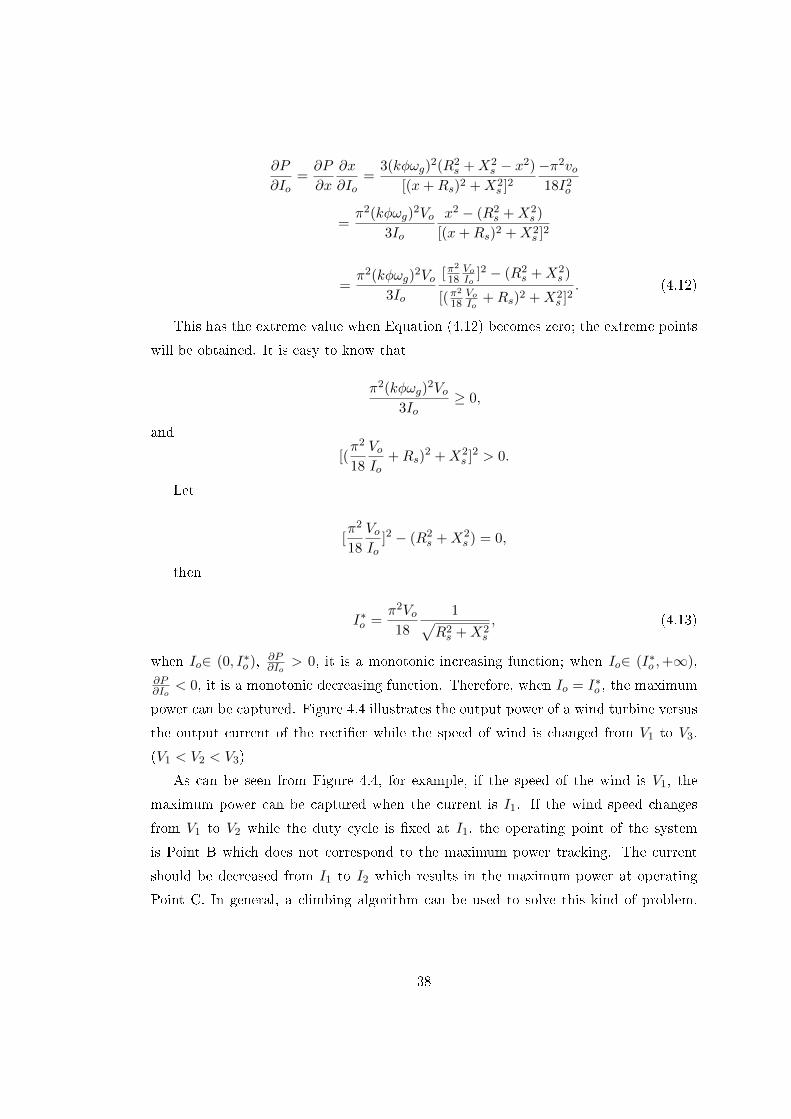
∂P
∂Io=∂P
∂x
∂x
∂Io=
3(kφωg)2(R2
s +X2s − x2)
[(x+Rs)2 +X2s ]2
−π2vo18I2
o
=π2(kφωg)
2Vo3Io
x2 − (R2s +X2
s )
[(x+Rs)2 +X2s ]2
=π2(kφωg)
2Vo3Io
[π2
18VoIo
]2 − (R2s +X2
s )
[(π2
18VoIo
+Rs)2 +X2s ]2
. (4.12)
This has the extreme value when Equation (4.12) becomes zero; the extreme points
will be obtained. It is easy to know that
π2(kφωg)2Vo
3Io≥ 0,
and
[(π2
18
VoIo
+Rs)2 +X2
s ]2 > 0.
Let
[π2
18
VoIo
]2 − (R2s +X2
s ) = 0,
then
I∗o =π2Vo18
1√R2s +X2
s
, (4.13)
when Io∈ (0, I∗o ), ∂P∂Io
> 0, it is a monotonic increasing function; when Io∈ (I∗o ,+∞),∂P∂Io
< 0, it is a monotonic decreasing function. Therefore, when Io = I∗o , the maximum
power can be captured. Figure 4.4 illustrates the output power of a wind turbine versus
the output current of the rectier while the speed of wind is changed from V1 to V3.
(V1 < V2 < V3)
As can be seen from Figure 4.4, for example, if the speed of the wind is V1, the
maximum power can be captured when the current is I1. If the wind speed changes
from V1 to V2 while the duty cycle is xed at I1, the operating point of the system
is Point B which does not correspond to the maximum power tracking. The current
should be decreased from I1 to I2 which results in the maximum power at operating
Point C. In general, a climbing algorithm can be used to solve this kind of problem.
38

P
V3
C V2
B
V1
A
I1 I2 Io
Figure 4.4: Power versus output current of a rectier for three dierent wind speeds.
Algorithm 4.1 Climbing algorithm (modied from [21])1) Measure the output power P = V I and increase the reference current by one step2) Measure the output power again.3) Calculate 4P and 4I.4) I∗(n) = I∗(n− 1) + Istep
∆P∆I .
5) Repeat from Step 2 to reach to the optimum operating point.Where V , I are the output voltage and current of the rectier, respectively.
This climbing algorithm, which adopts the dierent steps according to ∆P∆I , is shown in
Algorithm 4.1. In this way, it will make the system respond quickly.
The output current of the rectier should be controlled to track the reference current
that is obtained from the climbing algorithm. As a result, the maximum power will be
captured. The basic structure and control topology of the boost converter is shown in
Figure 4.5. The transfer function of a PI controller is given by
CPI(s) = Kp +Ki
s, (4.14)
where Kp and Ki are proportional and integral gains respectively.
4.3 Simulation Results
4.3.1 Model of a wind turbine
The wind turbine model is shown in the following scheme (see Figure 4.6).
The tip speed ratio λ is calculated in the rst subsystem using
39

Climbing Algorithm PIPWM
Generator
I*
I
VPWM
+ - p
Figure 4.5: Control strategy.
Tm
1
Turbine torque
v
w
Cp
p
R
Tm
Tip speed ratio
v
w
R
Lambda
Power coefficient
Lambda Cp
Air density
1.20
w
3
R
2
wind speed
1
Figure 4.6: Wind turbine model.
λ =Rω
v.
where R is the radius of the blades; v is the wind speed; and ω is the rotation speed of
the rotor.
The power coecient Cp value is calculated in the next subsystem by using the
following formulas [23]:
Cp(β, θ) = 0.22(116
β− 0.4θ − 5)e
− 12.5β
and
β =1
1λ+0.08θ −
0.035θ3+1
.
Cp depends on the tip speed ratio λ of the wind turbine and the angle of blades β.
The wind turbine extracts power from the wind and then converts it into mechanical
40
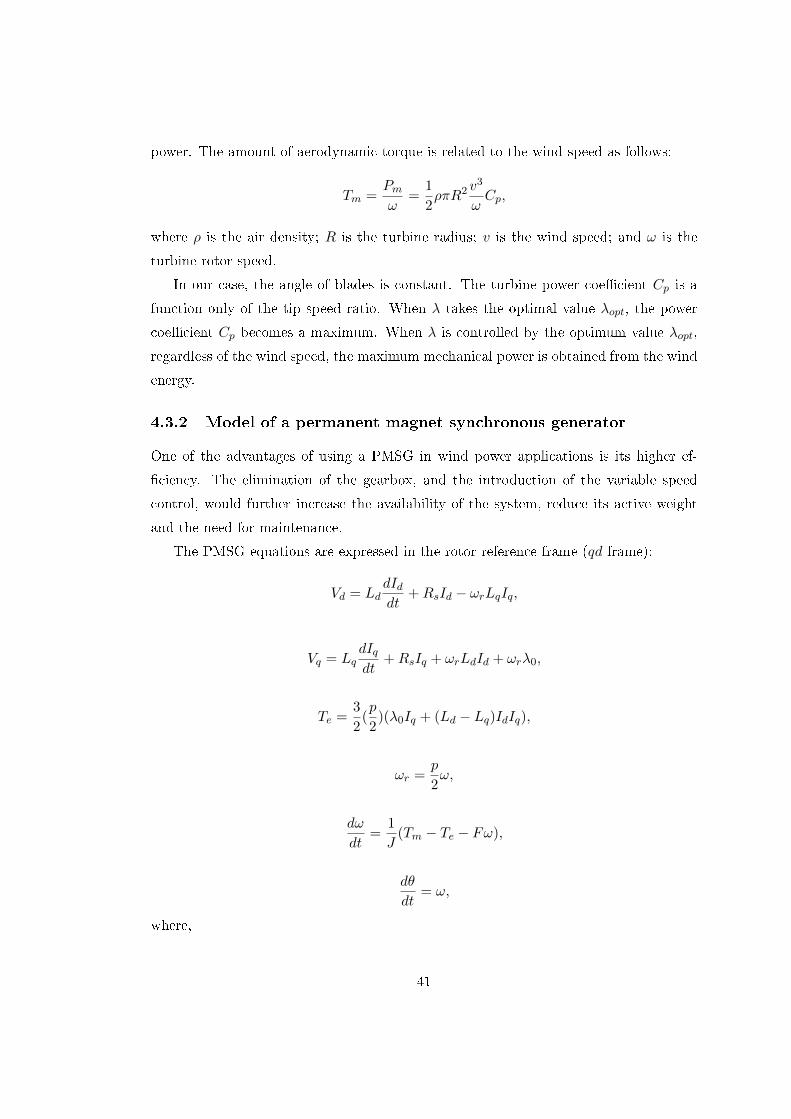
power. The amount of aerodynamic torque is related to the wind speed as follows:
Tm =Pmω
=1
2ρπR2 v
3
ωCp,
where ρ is the air density; R is the turbine radius; v is the wind speed; and ω is the
turbine rotor speed.
In our case, the angle of blades is constant. The turbine power coecient Cp is a
function only of the tip speed ratio. When λ takes the optimal value λopt, the power
coecient Cp becomes a maximum. When λ is controlled by the optimum value λopt,
regardless of the wind speed, the maximum mechanical power is obtained from the wind
energy.
4.3.2 Model of a permanent magnet synchronous generator
One of the advantages of using a PMSG in wind power applications is its higher ef-
ciency. The elimination of the gearbox, and the introduction of the variable speed
control, would further increase the availability of the system, reduce its active weight
and the need for maintenance.
The PMSG equations are expressed in the rotor reference frame (qd frame):
Vd = LddIddt
+RsId − ωrLqIq,
Vq = LqdIqdt
+RsIq + ωrLdId + ωrλ0,
Te =3
2(p
2)(λ0Iq + (Ld − Lq)IdIq),
ωr =p
2ω,
dω
dt=
1
J(Tm − Te − Fω),
dθ
dt= ω,
where,
41

Table 4.1: Parameters of the PMSG.
Parameters Values Parameters ValuesLd 0.975mH Lq 0.975mHRs 0.0918Ω Flux linkage 0.1688V.s
Inertial 3.94e-3kg.m2 Friction 4.924e-4N.m.sPole pairs 4 Ts 1e− 6
Lq, Ld: q and d axis inductances
R: Resistance of the stator windings
Iq, Id: q and d axis currents
Vq, Vd: q and d axis voltages
ωr: Angular velocity of the rotor
λ0: Amplitude of the ux induced by the permanent magnets of the rotor in the
stator phases
p: Number of pole pairs
Te: Electromagnetic torque
ω: Rotation speed of the rotating frame.
The Park transformation is commonly used in three-phase electric machine models.
It transforms from a three-phase (abc) reference frame to a dq0 reference frame. The
following transformations are used
Id =2
3(Iacosθ + Ibcos(θ −
2
3π) + Iccos(θ +
2
3π)),
Iq =2
3(Iasinθ + Ibsin(θ − 2
3π) + Icsin(θ +
2
3π)).
The Clarke transformation transforms it from a dq0 reference frame to a three-phase
(abc) reference frame. The following transformations are used
Va = Vdcosθ − Vqsinθ,
Vb = Vdcos(θ −2
3π)− Vqsin(θ − 2
3π),
Vc = Vdcos(θ +2
3π)− Vqsin(θ +
2
3π),
42
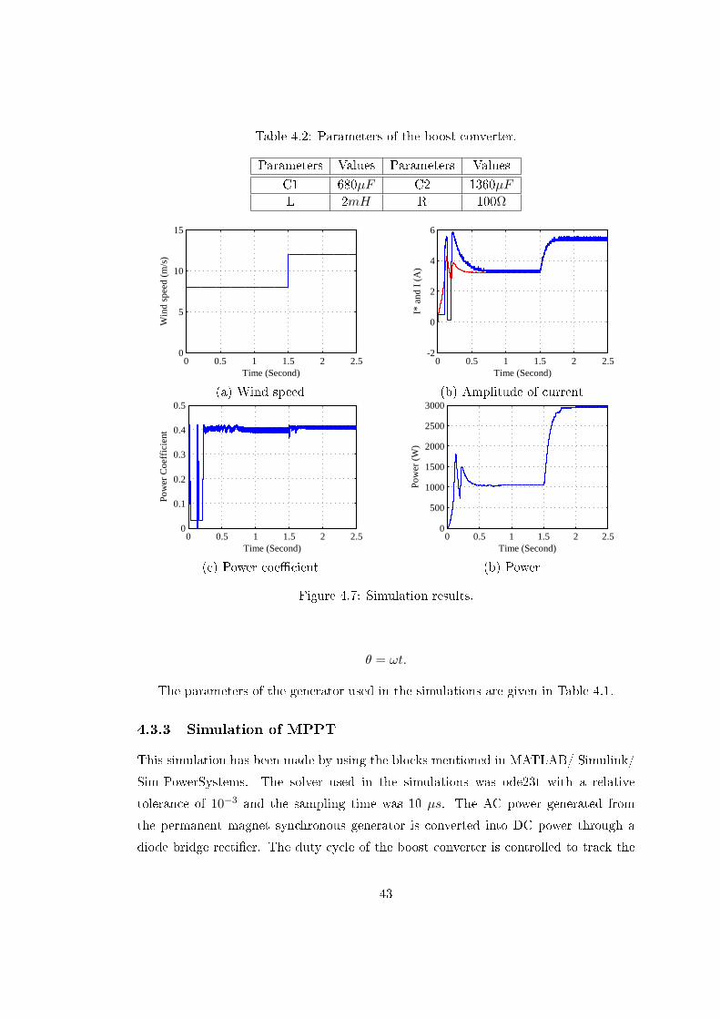
Table 4.2: Parameters of the boost converter.
Parameters Values Parameters ValuesC1 680µF C2 1360µFL 2mH R 100Ω
0 0.5 1 1.5 2 2.50
5
10
15
Time (Second)
Win
d sp
eed
(m/s
)
0 0.5 1 1.5 2 2.5-2
0
2
4
6
Time (Second)
I* a
nd I
(A
)
(a) Wind speed (b) Amplitude of current
0 0.5 1 1.5 2 2.50
0.1
0.2
0.3
0.4
0.5
Time (Second)
Pow
er C
oeff
icie
nt
0 0.5 1 1.5 2 2.50
500
1000
1500
2000
2500
3000
Time (Second)
Pow
er (
W)
(c) Power coecient (b) Power
Figure 4.7: Simulation results.
θ = ωt.
The parameters of the generator used in the simulations are given in Table 4.1.
4.3.3 Simulation of MPPT
This simulation has been made by using the blocks mentioned in MATLAB/ Simulink/
Sim-PowerSystems. The solver used in the simulations was ode23t with a relative
tolerance of 10−3 and the sampling time was 10 µs. The AC power generated from
the permanent magnet synchronous generator is converted into DC power through a
diode bridge rectier. The duty cycle of the boost converter is controlled to track the
43

Figure 4.8: Experimental setup.
reference current generated by the climbing algorithm.
The parameters of the boost converter used in the simulations are given in Table
9.1.
The simulation was started at t = 0. The initial time is from t = 0 to 0.2s, so the
rst 0.2 second is ignored in our analysis. The wind speed was changed from 8 to 12m/s
at t = 1.5s. The simulations were carried out in Matlab7.6/Simulink. The solver used
in the simulations was ode23t with a relative tolerance of 10−3 and a maximum step
size of 10 µs.
The simulation results are shown in Figure 4.7. The output current of the rectier
I (blue line) tracked the reference current I∗ (red line) very well in (b). The power
coecient Cp was at almost maximum all the time, regardless of the wind speed in (c).
The system responses were stable and very quick. When the wind speed was changed
from 8 to 12 m/s at t=1.5s, the power was increased from 1000 to 2900W in 0.3 second.
4.4 Experimental Results
The experimental setup, shown in Figure 4.8, consists of a I/O conditioning board,
a measurement transducers board, a boost converter board, an LCL lter board, a
Semistack IGBT device consisting of an uncontrollable rectier and an inverter, a
44

Figure 4.9: The experimental topology for MPPT.
TMS320F28335 digital signal controller and a Code Composer Studio, and MATLAB
Simulink/ SimPowerSystems Package and Target Support Package TC2.
The speed controllable induction motor has been used as a wind turbine in the ini-
tial experiments. The AC power generated from the permanent magnet synchronous
generator is converted into DC power through the diode bridge rectier. In the DC
bus, a boost converter has been used to achieve maximum power point tracking. Be-
cause the duty cycle of the boost converter is the only control variable, and the real
power measured at the converter output is considered, normally used inverters or en-
ergy storages will not take simplicity into account, so instead a resistor is connected
directly. The resistor provides a virtual load for consuming the real power generation.
The experimental topology is shown in Figure 4.9.
Experimental results (see Figure 4.10) have been obtained from Code Composer
Studio 3.3 in real time mode. In Figure 4.10 the left column shows the experimental
results when the induction motor was operated at 300rpm. The reference I∗ and the
actual I are around 1.04. The duty cycle D is around 29.6%. Reference I∗, actual I
and duty cycle D were changed in Figure 4.10's right column when the induction motor
was operated at 150rpm.
4.5 Conclusions
In this chapter, a simple MPPT control scheme is proposed for the wind turbine applica-
tion without mechanical sensors by using a climbing algorithm and a PI controller. Both
simulation and experimental results are provided to conrm that the control strategy
works well to track the maximum power for dierent wind speeds.
45

(a) Reference current
(b) Inductor current
(c) Duty cycle
Figure 4.10: Experimental results: for the case with 300rpm (left column) and 150rpm(right column).
46

Chapter 5
Overview of the Synchronverter
Technology
Power systems currently receive more and more contributions from distributed energy
sources, in particular, from renewable energy sources. Renewable energy sources are
uncontrollable and highly non-linear. If their share in a power system becomes signi-
cant, a modem control strategy is required not only to preserve, but also to improve
the stability of the power system. It is one of the biggest challenges for all researchers
working in this area to propose the most ecient way to send renewable power to the
grid without degrading the system stability.
In general, the control schemes for sending power from a renewable energy source
to the utility grid are quite similar and include two stages. In the rst stage, the source
power is converted into electrical power, often in the form of DC, using appropriate
techniques. The second stage is to feed the electrical power to the utility grid, often via
DC-AC converters, also called inverters. Various control strategies can be applied at
this stage to control the power owing into the grid from the DC bus. Dierent control
strategies have dierent ways of feeding the power to the grid and therefore the impact
on the stability of the power system is dierent.
Dierent control methods can be applied at the second stage to control grid-connected
inverters. The two most-studied methods are power (torque) angle control and current
vector control for voltage source inverters (VSI). Generally, the current vector control
method aims at delivering current ows with low harmonic distortion to the grid while
maintaining a stable DC bus voltage [24, 25, 26, 27]. Because the source model for the
inverter in this method is a current source mode [28], maintaining the DC bus voltage
47
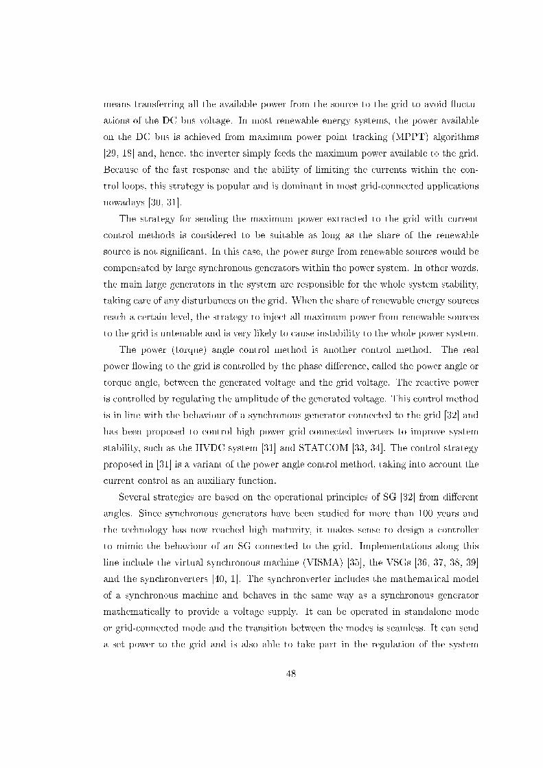
means transferring all the available power from the source to the grid to avoid uctu-
ations of the DC bus voltage. In most renewable energy systems, the power available
on the DC bus is achieved from maximum power point tracking (MPPT) algorithms
[29, 18] and, hence, the inverter simply feeds the maximum power available to the grid.
Because of the fast response and the ability of limiting the currents within the con-
trol loops, this strategy is popular and is dominant in most grid-connected applications
nowadays [30, 31].
The strategy for sending the maximum power extracted to the grid with current
control methods is considered to be suitable as long as the share of the renewable
source is not signicant. In this case, the power surge from renewable sources would be
compensated by large synchronous generators within the power system. In other words,
the main large generators in the system are responsible for the whole system stability,
taking care of any disturbances on the grid. When the share of renewable energy sources
reach a certain level, the strategy to inject all maximum power from renewable sources
to the grid is untenable and is very likely to cause instability to the whole power system.
The power (torque) angle control method is another control method. The real
power owing to the grid is controlled by the phase dierence, called the power angle or
torque angle, between the generated voltage and the grid voltage. The reactive power
is controlled by regulating the amplitude of the generated voltage. This control method
is in line with the behaviour of a synchronous generator connected to the grid [32] and
has been proposed to control high power grid-connected inverters to improve system
stability, such as the HVDC system [31] and STATCOM [33, 34]. The control strategy
proposed in [31] is a variant of the power angle control method, taking into account the
current control as an auxiliary function.
Several strategies are based on the operational principles of SG [32] from dierent
angles. Since synchronous generators have been studied for more than 100 years and
the technology has now reached high maturity, it makes sense to design a controller
to mimic the behaviour of an SG connected to the grid. Implementations along this
line include the virtual synchronous machine (VISMA) [35], the VSGs [36, 37, 38, 39]
and the synchronverters [40, 1]. The synchronverter includes the mathematical model
of a synchronous machine and behaves in the same way as a synchronous generator
mathematically to provide a voltage supply. It can be operated in standalone mode
or grid-connected mode and the transition between the modes is seamless. It can send
a set power to the grid and is also able to take part in the regulation of the system
48
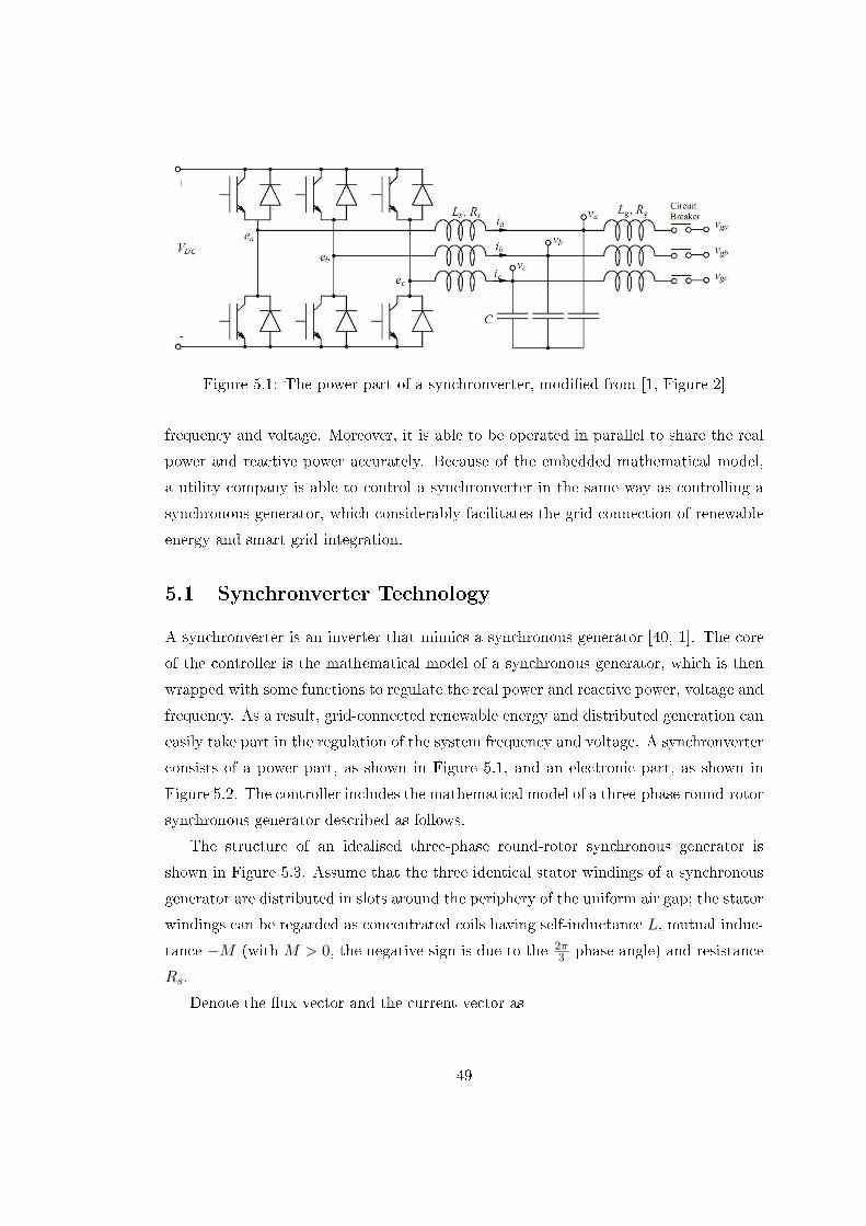
Figure 5.1: The power part of a synchronverter, modied from [1, Figure 2]
frequency and voltage. Moreover, it is able to be operated in parallel to share the real
power and reactive power accurately. Because of the embedded mathematical model,
a utility company is able to control a synchronverter in the same way as controlling a
synchronous generator, which considerably facilitates the grid connection of renewable
energy and smart grid integration.
5.1 Synchronverter Technology
A synchronverter is an inverter that mimics a synchronous generator [40, 1]. The core
of the controller is the mathematical model of a synchronous generator, which is then
wrapped with some functions to regulate the real power and reactive power, voltage and
frequency. As a result, grid-connected renewable energy and distributed generation can
easily take part in the regulation of the system frequency and voltage. A synchronverter
consists of a power part, as shown in Figure 5.1, and an electronic part, as shown in
Figure 5.2. The controller includes the mathematical model of a three-phase round-rotor
synchronous generator described as follows.
The structure of an idealised three-phase round-rotor synchronous generator is
shown in Figure 5.3. Assume that the three identical stator windings of a synchronous
generator are distributed in slots around the periphery of the uniform air gap; the stator
windings can be regarded as concentrated coils having self-inductance L, mutual induc-
tance −M (with M > 0, the negative sign is due to the 2π3 phase angle) and resistance
Rs.
Denote the ux vector and the current vector as
49

1Ks 1s Reset 1Js
Q
Qref Mfif Te Tm θ
θc vg
i
Eqn.(5.2) Eqn.(5.4) Eqn.(5.5) Dp
Pref
v Amplitude Detection vr vm
e
θɺ 1nθɺ
Dq
θɺ r
Figure 5.2: The electronic part (controller) of a synchronverter, modied from [1, Figure3]
Φ =
Φa
Φb
Φc
, i =
ia
ib
ic
,respectively, and the vectors
cosθ =
cosθ
cos(θ − 2π3 )
cos(θ − 4π3 )
, sinθ =
sinθ
sin(θ − 2π3 )
sin(θ − 4π3 )
,where θ is the rotor angle with respect to the Phase A winding. Then the phase terminal
voltages v = [ va vb vc ]T of a generator can be written as
v = e−Rsi− Lsdi
dt, (5.1)
where Ls = L+M and e = [ ea eb ec ]T is the back EMF due to the rotor movement
given by
e = Mf if θsinθ −Mfdifdt
cosθ. (5.2)
The mechanical part of the generator is governed by
50

a-axis
Rotor field axis θ sR , sL ai
av
fi fR , fL M
Field voltage fv
bv cv
bi ci
b-axis c-axis
Figure 5.3: Structure of an idealized three-phase round-rotor synchronous generator,modied from [1, Figure 1]
θ =1
J(Tm − Te −Dpθg), (5.3)
where J is the moment of inertia of all the parts rotating with the rotor; Dp is a damping
factor; Tm is the mechanical torque and Te is the electromagnetic torque
Te = Mf if
⟨i, sinθ
⟩, (5.4)
where 〈·, ·〉 denotes the conventional inner product in R3.
The real power and reactive power are, respectively,
P = θMfif < i, sinθ >,
Q = −θMfif < i, cosθ > . (5.5)
Similarly to the control of a synchronous generator, the controller of a synchronverter
has two channels: one for the real power and the other for the reactive power. The
real power is controlled by a frequency droop control loop, which is implemented in a
synchronverter by comparing the virtual angular speed θ with the angular frequency
51
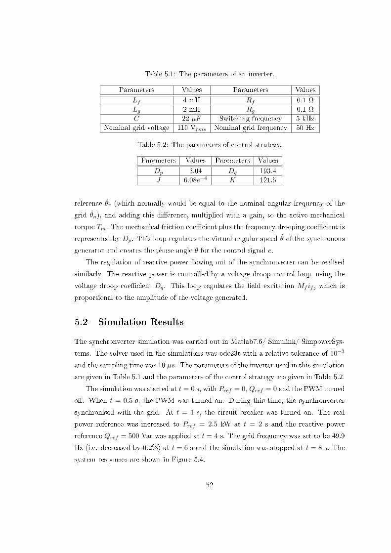
Table 5.1: The parameters of an inverter.
Parameters Values Parameters ValuesLf 4 mH Rf 0.1 Ω
Lg 2 mH Rg 0.1 Ω
C 22 µF Switching frequency 5 kHzNominal grid voltage 110 Vrms Nominal grid frequency 50 Hz
Table 5.2: The parameters of control strategy.
Paremeters Values Paremeters ValuesDp 3.04 Dq 193.4J 6.08e−4 K 121.5
reference θr (which normally would be equal to the nominal angular frequency of the
grid θn), and adding this dierence, multiplied with a gain, to the active mechanical
torque Tm. The mechanical friction coecient plus the frequency drooping coecient is
represented by Dp. This loop regulates the virtual angular speed θ of the synchronous
generator and creates the phase angle θ for the control signal e.
The regulation of reactive power owing out of the synchronverter can be realised
similarly. The reactive power is controlled by a voltage droop control loop, using the
voltage droop coecient Dq. This loop regulates the eld excitation Mf if , which is
proportional to the amplitude of the voltage generated.
5.2 Simulation Results
The synchronverter simulation was carried out in Matlab7.6/ Simulink/ SimpowerSys-
tems. The solver used in the simulations was ode23t with a relative tolerance of 10−3
and the sampling time was 10 µs. The parameters of the inverter used in this simulation
are given in Table 5.1 and the parameters of the control strategy are given in Table 5.2.
The simulation was started at t = 0 s, with Pref = 0, Qref = 0 and the PWM turned
o. When t = 0.5 s, the PWM was turned on. During this time, the synchronverter
synchronised with the grid. At t = 1 s, the circuit breaker was turned on. The real
power reference was increased to Pref = 2.5 kW at t = 2 s and the reactive power
reference Qref = 500 Var was applied at t = 4 s. The grid frequency was set to be 49.9
Hz (i.e. decreased by 0.2%) at t = 6 s and the simulation was stopped at t = 8 s. The
system responses are shown in Figure 5.4.
52

0 1 2 3 4 5 6 7 8313
314
315
316
317
318
Time [s]
Freq
uenc
y [r
ad/s
]
θg θ
0 1 2 3 4 5 6 7 80
20406080
100120140160
Time [s]
rms
[V]
v
rmsirms
(a) Frequency (b) Amplitude of v − vg
0 1 2 3 4 5 6 7 8−500
0500
1000150020002500300035004000
Time [s]
P ref a
nd P
[W]
P
ref P
0 1 2 3 4 5 6 7 8−250
0
250
500
750
1000
Time [s]
Qre
f and
Q [V
ar]
Q
ref Q
(c) Real power (d) Reactive power
Figure 5.4: Simulation results
As shown in Figure 5.4(a), regardless of the reference Pref and Qref applied, the
synchronverter tracked the grid frequency very well, even when the frequency decreased
by 0.1 Hz at t = 6 s. Moreover, the real power and the reactive power tracked their
references quickly and accurately under dierent operational conditions, as shown in
Figure 5.4(c) and (d).
Figure 5.5 shows the grid voltage va and the control signal ea in the dierent cases.
Obviously, there were no big dierences between the cases of before connection and after
connection. The control signal ea was synchronised with the grid voltage va (in terms
of phase and frequency). When Pref = 2.5 kW, the control signal ea had a small phase
shift with the grid voltage va in Figure 5.5(c). Moreover, when Qref = 500 Var, the
control signal ea increased slightly in Figure 5.5(d). It means that the real power and
the reactive power are controlled by the frequency droop control loop and the voltage
droop control loop, respectively.
5.3 Experimental Results
Experiments were also carried out on the experimental setup which is described in the
previous chapter. The speed controllable induction motor was used to drive the per-
53
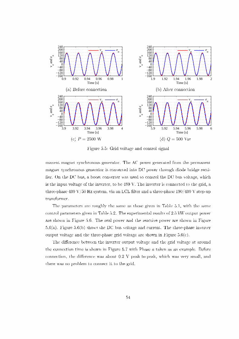
0.9 0.92 0.94 0.96 0.98 1−160−120−80−40
04080
120160200240
Time [s]
v a and
e a
v
ae
a
1.9 1.92 1.94 1.96 1.98 2−160−120−80−40
04080
120160200240
Time [s]
v a and
e a
v
ae
a
(a) Before connection (b) After connection
3.9 3.92 3.94 3.96 3.98 4−160−120−80−40
04080
120160200240
Time [s]
v a and
e a
v
ae
a
5.9 5.92 5.94 5.96 5.98 6−160−120−80−40
04080
120160200240
Time [s]
v a and
e a
v
ae
a
(c) P = 2500 W (d) Q = 500 Var
Figure 5.5: Grid voltage and control signal
manent magnet synchronous generator. The AC power generated from the permanent
magnet synchronous generator is converted into DC power through diode bridge recti-
er. On the DC bus, a boost converter was used to control the DC bus voltage, which
is the input voltage of the inverter, to be 480 V. The inverter is connected to the grid, a
three-phase 400 V/50 Hz system, via an LCL lter and a three-phase 190/400 V step-up
transformer.
The parameters are roughly the same as those given in Table 5.1, with the same
control parameters given in Table 5.2. The experimental results of 2.5 kW output power
are shown in Figure 5.6. The real power and the reactive power are shown in Figure
5.6(a). Figure 5.6(b) shows the DC bus voltage and current. The three-phase inverter
output voltage and the three-phase grid voltage are shown in Figure 5.6(c).
The dierence between the inverter output voltage and the grid voltage at around
the connection time is shown in Figure 5.7 with Phase a taken as an example. Before
connection, the dierence was about 0.2 V peak-to-peak, which was very small, and
there was no problem to connect it to the grid.
54

(a) The real power and the reactive power
(b) The DC bus current and voltage
(c) the three-phase inverter output voltage and the three-phase grid voltage
Figure 5.6: 2.5kW experimental results
55

Figure 5.7: Error between output voltage and grid voltage
5.4 Conclusions
In this chapter, the synchronverter technology was introduced. It can be operated in
the standalone mode or the grid-connected mode and the transition between the modes
is seamless. It is able to send a set power to the grid and is also able to take part in
the regulation of the system frequency and voltage. Moreover, it can be operated in
parallel to share the real power and reactive power accurately. Both simulation and
experimental results were provided.
56

Chapter 6
Synchronverters in Parallel
Operation
As mentioned in the previous chapter, synchronverters can be operated in parallel to
share the real power and reactive power accurately because of the voltage and frequency
droop control method. In this chapter, the speciality of synchronverters with parallel
operation was discussed and a synchronverter-based control scheme for parallel inverters
was proposed.
Rapidly increasing DPGS based on renewable energy are connected to the public
grid via power inverters. They often form microgrids before being connected to the
utility grid [41, 42, 43, 44, 45]. Due to the availability of high current power electronic
devices, it is inevitable that multiple inverters are needed to be operated in parallel
for high-power and/or low-cost application. Additionally, inverters are widely used
in stand-alone mode, such as UPS, energy storage systems and backup power supply
systems. These applications can be implemented by using a high-capacity inverter
or several low-capacity inverters. It is well-known that the use of a singular high-
capacity inverter has many disadvantages [46]. In other words, the parallel operation of
several low-capacity inverters is better than a singular high-capacity inverter due to the
advantages of better extensibility and reliability. Consequently, the inverter that gives
the performance of parallel operation is an important trend.
The conventional control methods for parallel-connected inverters can be classied
into two types. One is the active current distribution type which uses active current
distribution control to adapt the current-mode control. The object of the active cur-
rent distribution control is to generate a reference current for each parallel-connected
57

1s1Js
Mfif Te θ
i
Eqn.(5.2) Eqn.(5.4) Dp
v Amplitude Detection vref vm
e
θɺ
Dq
θɺ ref
1KsFigure 6.1: Proposed control scheme for parallel operation
inverter, and it can be subdivided into three methods: the master-slave control method
[46, 47, 48], the concentrated distribution control method [49, 50] and the ring control
method [51]. Another is the droop control [52, 53, 54, 55, 56, 57, 58, 59, 1], which is
widely used in conventional power generation systems [60]. The advantage is that no
external communication mechanism is needed among the inverters to share the load
automatically [57, 61]. This enables good sharing for linear and/or nonlinear loads
[62, 63, 64, 65, 66]. In some cases, external communication means are still adopted for
load sharing [67] and restoring the microgrid voltage and frequency.
6.1 Description of the Control Scheme
A parallel operation control strategy based on synchronverters was proposed in Figure
6.1. In comparison to the synchronverter (see Figure 5.2), Pset and Q loop are removed
from the controller. The real power is controlled by a frequency droop control loop,
which is implemented in a synchronverter by comparing the virtual angular speed θ
with the angular frequency reference θref , and adding this dierence, multiplied with a
gain, to the active mechanical torque Tm. This loop regulates the virtual angular speed
θ of the synchronous generator and creates the phase angle θ for the control signal e.
The mechanical friction coecient plus the frequency drooping coecient is represented
58

Table 6.1: The parameters used in the simulation.
Parameters Values Parameters ValuesDp1 6.08 Dp2 3.04Dq1 385.7 Dq2 192.8J1 0.0122 J2 0.0061K1 242.34 K2 121.17
by Dp. Dening the frequency drooping coecient Dp as the change in the total torque
acting on the imaginary rotor ∆T and the change in angular frequency ∆θ gives:
Dp = −∆T
∆θ.
The regulation of reactive power owing out of the synchronverter can be realised
similarly. This loop regulates the eld excitation Mf if , which is proportional to the
amplitude of the voltage generated. The reactive power is controlled by a voltage droop
control loop, using the voltage droop coecient Dq. Dening the voltage drooping
coecient Dq as the ratio of the required change of reactive power ∆Q to the change
of voltage ∆v gives:
Dq = −∆Q
∆v.
6.2 Simulation Results
A system that consists of two three-phase inverters powered by two separate 400 V DC
voltage supplies was used to carry out simulations to verify the control strategy. The
simulations were carried out in Matlab7.6/ Simulink/ SimpowerSystems. The solver
used in the simulations was ode23t with a relative tolerance of 10−3 and the sampling
time was 10 µs. The rated voltage is 110V and the frequency of the system is 50Hz. The
lter inductor is L = 2.2mH with a parasitic resistance of 0.1Ω and the lter capacitance
C is 22µF.
6.2.1 With a linear load
The capacity of Inverter 1 is 3000VA and the capacity of Inverter 2 is 1500VA. The
parameters of simulation are shown in Table 6.1. Simulation was carried out for a
59

0.5 0.52 0.54 0.56 0.58 0.6−20
−10
0
10
20
30
Time [s]
Cur
rent
[A]
i1
i2 i
0 0.2 0.4 0.6 0.8 1 1.2 1.4 1.6 1.8 20
4
8
12
16
20
Time [s]
Cur
rent
[A
]
irms1
irms2
irms
(a) Current i1, i2 and i (b) RMS current irms1, irms2 and irms
1.9 1.92 1.94 1.96 1.98 2−200−150−100−50
050
100150200
Vol
tage
[V]
Time [s]0 0.2 0.4 0.6 0.8 1 1.2 1.4 1.6 1.8 2
020406080
100120140
Vol
tage
[V
]
Time [s]
(c) Load voltage (d) RMS voltage of load
0 0.2 0.4 0.6 0.8 1 1.2 1.4 1.6 1.8 20
1000
2000
3000
4000
Time [s]
P [W
]
P
1P
2
0 0.2 0.4 0.6 0.8 1 1.2 1.4 1.6 1.8 2−150−100−50
050
100150200250
Time [s]
Q [V
ar]
Q
1Q
2
(e) Real power P1 and P2 (f) Reactive power Q1 and Q2
0 0.2 0.4 0.6 0.8 1 1.2 1.4 1.6 1.8 249.5
49.5549.6
49.6549.7
49.7549.8
49.8549.9
49.9550
Time [s]
Q [
Var
]
f1
f2
0 0.2 0.4 0.6 0.8 1 1.2 1.4 1.6 1.8 20
1
2
3
4
5
TH
D [
%]
Time [s]
(g) Frequency f1 and f2 (h) THD of load voltage
Figure 6.2: Simulation results with a linear load
60

linear load with R = 9Ω for each phase. The system responses are shown in Figure
6.2. It can been seen that the parallel operation of two inverters performed very well.
The current of Inverter 1, Inverter 2 and load are shown in Figure 6.2 (a) with Phase A
taken as an example. They are nearly sinusoidal with little phase shift between them
and irms1 + irms2 = irms. The output voltage is very close to the rated voltage 110V
with low THD (about 1.1%). The real power and reactive power are well shared.
6.2.2 With a nonlinear load
The same simulations were carried out for a full-bridge rectier load with an LC lter
L = 150µH, C = 1000µF and R = 9Ω. The system responses are shown in Figure 6.3.
While this appliance consumes the real power, as it is a nonlinear load, it also outputs
harmonics and consumes the reactive power. The real power and reactive power were
accurately shared. The load voltage is close to the rated voltage with 21% THD.
6.2.3 Master-slave mode with a linear load
A master-slave architecture of an inverter system is presented which allows parallel
operation of an arbitrary number of inverter modules by a simple control method. The
simulation of master-slave mode was also carried out. The proposed control scheme was
applied for Inverter 1 as the master mode. Inverter 2 is a synchronverter which means
that Inverter 2 can track the master phase by a synchronisation unit and can also set
the real power and reactive power references.
The simulation was started at t = 0s, with the Circuit breaker S o. At t = 1s,
the Circuit breaker S was on and Inverter 2 was connected to the load. Meanwhile,
the real power reference P2 was 1000W and the reactive power reference Q2 was zero.
Then, P2 was changed to 1500W at t = 2s and Q2 was changed to 500Var at t = 3s.
The system responses are shown in Figure 6.4. The parallel operation of two inverters
performed very well. The real power and reactive power were accurately shared with
P = P1 + P2 and Q = Q1 + Q2. P2 tracked the reference very well and P1 shared the
load automatically. The load voltage is stable and purely sinusoidal, even when the
state of the inverters changed.
The current of Inverter 1, Inverter 2 and the load in dierent situations are shown in
Figure 6.5. When Circuit breaker S was o, the current of Inverter 1 i1 is exactly equal
to the current of the load i. When P2 = 1000W or P2 = 1500W, the Inverter 1 current
61

0.5 0.52 0.54 0.56 0.58 0.6−40
−20
0
20
40
60
Time [s]
Cur
rent
[A]
i1
i2 i
0 0.2 0.4 0.6 0.8 1 1.2 1.4 1.6 1.8 205
101520253035
Time [s]
Cur
rent
[A
]
irms1
irms2
irms
(a) Current i1, i2 and i (b) RMS current irms1, irms2 and irms
1.9 1.92 1.94 1.96 1.98 2−200−150−100−50
050
100150200
Vol
tage
[V]
Time [s]0 0.2 0.4 0.6 0.8 1 1.2 1.4 1.6 1.8 2
020406080
100120140
Vol
tage
[V
]
Time [s]
(c) Load voltage (d) RMS voltage of load
0 0.2 0.4 0.6 0.8 1 1.2 1.4 1.6 1.8 20
1000
2000
3000
4000
5000
6000
Time [s]
P [W
]
P
1P
2
0 0.2 0.4 0.6 0.8 1 1.2 1.4 1.6 1.8 2
0200400600800
10001200
Time [s]
Q [
Var
]
Q
1Q
2
(e) Real power P1 and P2 (f) Reactive power Q1 and Q2
0 0.2 0.4 0.6 0.8 1 1.2 1.4 1.6 1.8 249
49.2
49.4
49.6
49.8
50
Time [s]
Q [
Var
]
f1
f2
0 0.2 0.4 0.6 0.8 1 1.2 1.4 1.6 1.8 20
10
20
30
40
50
TH
D [
%]
Time [s]
(g) Frequency f1 and f2 (h) THD of load voltage
Figure 6.3: Simulation results with a nonlinear load
62

0 0.5 1 1.5 2 2.5 3 3.5 40
4
8
12
16
20
Time [s]
Cur
rent
[A
]
irms1
irms2
irms
0 0.5 1 1.5 2 2.5 3 3.5 449
49.5
50
50.5
51
Time [s]
Q [
Var
]
f1
f2
(a) RMS current irms1, irms2 and irms (b) Frequency f1 and f2
1.96 1.98 2 2.02 2.04 2.06−200−150−100−50
050
100150200
Vol
tage
[V]
Time [s]0 0.5 1 1.5 2 2.5 3 3.5 4
020406080
100120140
Vol
tage
[V
]
Time [s]
(c) Load voltage (d) RMS voltage of load
0 0.5 1 1.5 2 2.5 3 3.5 40
1000
2000
3000
4000
5000
6000
Time [s]
P [W
]
P
1P
2
0 0.5 1 1.5 2 2.5 3 3.5 4−1000
−500
0
500
1000
1500
Time [s]
Q [V
ar]
Q
1Q
2
(e) Real power P1 and P2 (f) Reactive power Q1 and Q2
Figure 6.4: Simulation results in the master-slave mode with a linear load
0.5 0.52 0.54 0.56 0.58 0.6−20
−10
0
10
20
30
Time [s]
Cur
rent
[A]
i1
i2 i
1.5 1.52 1.54 1.56 1.58 1.6−20
−10
0
10
20
30
Time [s]
Cur
rent
[A]
i1
i2 i
(a) When P2 = 0 W (b) When P2 = 1000 W
2.5 2.52 2.54 2.56 2.58 2.6−20
−10
0
10
20
30
Time [s]
Cur
rent
[A]
i1
i2 i
3.5 3.52 3.54 3.56 3.58 3.6−20
−10
0
10
20
30
Time [s]
Cur
rent
[A]
i1
i2 i
(b) When P2 = 1500 W (b) When Q2 = 500 Var
Figure 6.5: Current of inverter1, inverter2 and load
63
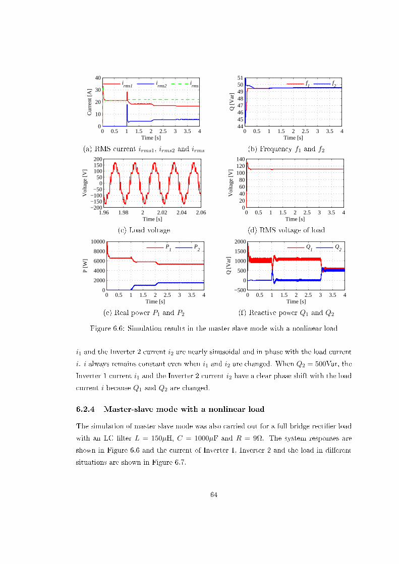
0 0.5 1 1.5 2 2.5 3 3.5 40
10
20
30
40
Time [s]
Cur
rent
[A
]
irms1
irms2
irms
0 0.5 1 1.5 2 2.5 3 3.5 44445464748495051
Time [s]
Q [
Var
]
f1
f2
(a) RMS current irms1, irms2 and irms (b) Frequency f1 and f2
1.96 1.98 2 2.02 2.04 2.06−200−150−100−50
050
100150200
Vol
tage
[V]
Time [s]0 0.5 1 1.5 2 2.5 3 3.5 4
020406080
100120140
Vol
tage
[V
]
Time [s]
(c) Load voltage (d) RMS voltage of load
0 0.5 1 1.5 2 2.5 3 3.5 40
2000
4000
6000
8000
10000
Time [s]
P [W
]
P
1P
2
0 0.5 1 1.5 2 2.5 3 3.5 4−500
0
500
1000
1500
2000
Time [s]
Q [V
ar]
Q
1Q
2
(e) Real power P1 and P2 (f) Reactive power Q1 and Q2
Figure 6.6: Simulation results in the master-slave mode with a nonlinear load
i1 and the Inverter 2 current i2 are nearly sinusoidal and in phase with the load current
i. i always remains constant even when i1 and i2 are changed. When Q2 = 500Var, the
Inverter 1 current i1 and the Inverter 2 current i2 have a clear phase shift with the load
current i because Q1 and Q2 are changed.
6.2.4 Master-slave mode with a nonlinear load
The simulation of master-slave mode was also carried out for a full-bridge rectier load
with an LC lter L = 150µH, C = 1000µF and R = 9Ω. The system responses are
shown in Figure 6.6 and the current of Inverter 1, Inverter 2 and the load in dierent
situations are shown in Figure 6.7.
64

0.5 0.52 0.54 0.56 0.58 0.6−40
−20
0
20
40
60
Time [s]
Cur
rent
[A]
i1
i2 i
1.5 1.52 1.54 1.56 1.58 1.6−40
−20
0
20
40
60
Time [s]
Cur
rent
[A]
i1
i2 i
(a) When P2 = 0 W (b) When P2 = 1000 W
2.5 2.52 2.54 2.56 2.58 2.6−40
−20
0
20
40
60
Time [s]
Cur
rent
[A]
i1
i2 i
3.5 3.52 3.54 3.56 3.58 3.6−40
−20
0
20
40
60
Time [s]C
urre
nt [A
]
i1
i2 i
(b) When P2 = 1500 W (b) When Q2 = 500 Var
Figure 6.7: Current of inverter1, inverter2 and load
6.3 Conclusions
In this chapter, a controller based on synchronverters for parallel inverters in stand-
alone mode has been proposed. The control strategy consists of a frequency droop
loop and a voltage droop loop which allow the sharing of the real power and reactive
power, respectively. Simulation results were provided to demonstrate the excellent
performance.
65

Chapter 7
Synchronverters with Capacitive
Output Impedances
Rapidly increasing energy consumption on one side and steadily reducing energy sources
on the other side, lead to the need for a DPGS based on renewable energy sources,
mainly from wind and solar energy [68, 69, 70]. They often form microgrids before
being connected to the utility grid [41, 71, 72, 73]. One of the major problems with
these applications is the quality of the microgrid voltage. For both wind turbines
and photovoltaics connected to the grid, the maximum limit for the Total harmonic
distortion of the output voltage is THD = 5% according to industrial regulations
[74, 75].
Several feedback control schemes, e.g. deadbeat or hysteresis controllers [76, 77],
have been proposed for inverters to reduce THD. However, these controllers alone cannot
eliminate the periodic distortion caused for example by nonlinear loads. Repetitive
control theory [78, 79], which is regarded as a simple learning control method, provides
an alternative for eliminating periodic errors in dynamic system, using the internal
model principle [80]. Furthermore, some research has been done on active lters [81, 82]
and grid-connected inverters [71, 74, 83].
The switching frequency of the PWM switching converter is usually a few kilohertz
and high-order frequency harmonics are small in magnitude and can be removed by a
lter. The lter is connected in parallel as an interface between the inverter and the
grid [84, 85, 86, 87, 88]. The output lter, used to reduce harmonic currents injected
into the grid or load, is a simple rst order L lter. However, implementation of LC
lters has been proposed to provide better harmonic attenuation and reduce the lter
66
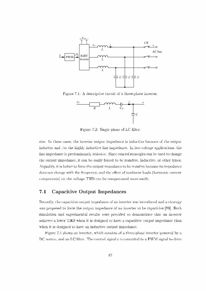
PWM
i
L
IGBT
Inverter
e
+ - V DC
e f
AC bus
C
CB v
L
L
C C
Figure 7.1: A descriptive circuit of a three-phase inverter.
L R C0
C
e f v i
Figure 7.2: Single phase of LC lter.
size. In these cases, the inverter output impedance is inductive because of the output
inductor and /or the highly inductive line impedance. In low-voltage applications, the
line impedance is predominantly resistive. Since control strategies can be used to change
the output impedance, it can be easily forced to be resistive, inductive, or other types.
Arguably, it is better to force the output impedance to be resistive because its impedance
does not change with the frequency, and the eect of nonlinear loads (harmonic current
components) on the voltage THD can be compensated more easily.
7.1 Capacitive Output Impedances
Recently, the capacitive output impedance of an inverter was introduced and a strategy
was proposed to force the output impedance of an inverter to be capacitive [89]. Both
simulation and experimental results were provided to demonstrate that an inverter
achieves a lower THD when it is designed to have a capacitive output impedance than
when it is designed to have an inductive output impedance.
Figure 7.1 shows an inverter, which consists of a three-phase inverter powered by a
DC source, and an LC lter. The control signal e is converted to a PWM signal to drive
67

1s1Js
vref Mfif Te Tm θ
i
Eqn.(5.2) Eqn.(5.4) Eqn.(5.5) fref
v Amplitude Detection e
θɺ 2π
ivKs
ifpf KK s+
1osC
er Figure 7.3: Control strategy based on synchronverters.
the inverter so that the average of ef over a switching period is the same as e. Figure
7.2 shows the single phase of LC lter. The following equation is easily obtained,
ef = (R+ sL+1
sC0)i+ v,
which gives
v = ef − Zo(s) · i,
where the output impedance Zo(s) is
Zo(s) = R+ sL+1
sC0.
When R is bigger than sL+ 1sC0
, the output impedance of the inverter can be treated
as resistive. When sL is bigger than R + 1sC0
, the output impedance of the inverter
can be treated as inductive. When 1sC0
is bigger than R + sL, the output impedance
of the inverter can be treated as capacitive. Therefore, if the capacitor C0 is chosen to
be small enough, the eect of the inductor (R + sL) is not signicant and the output
impedance can be made to be nearly purely capacitive at the fundamental frequency,
i.e., roughly
Zo(s) ≈1
sC0.
68
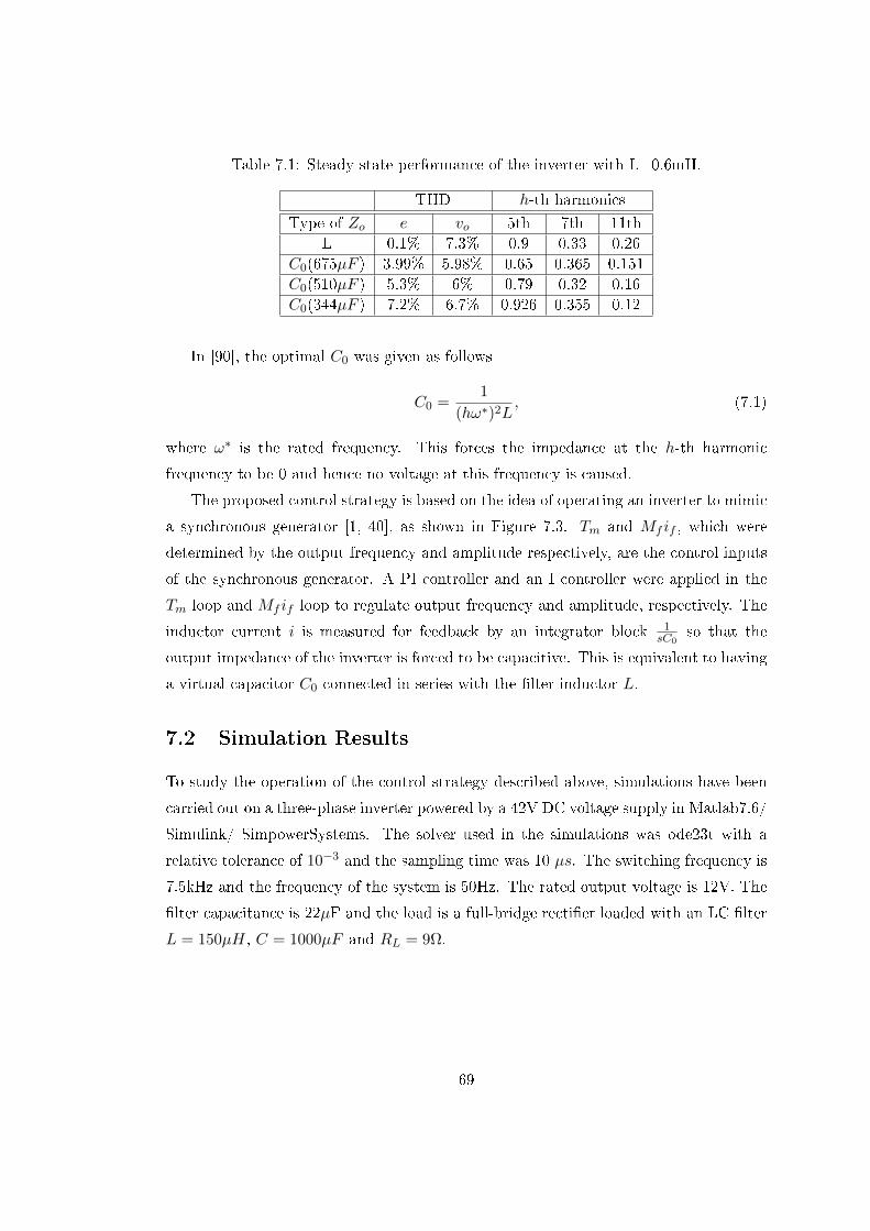
Table 7.1: Steady-state performance of the inverter with L=0.6mH.
THD h-th harmonicsType of Zo e vo 5th 7th 11th
L 0.1% 7.3% 0.9 0.33 0.26C0(675µF ) 3.99% 5.98% 0.65 0.365 0.151C0(510µF ) 5.3% 6% 0.79 0.32 0.16C0(344µF ) 7.2% 6.7% 0.926 0.355 0.12
In [90], the optimal C0 was given as follows
C0 =1
(hω∗)2L, (7.1)
where ω∗ is the rated frequency. This forces the impedance at the h-th harmonic
frequency to be 0 and hence no voltage at this frequency is caused.
The proposed control strategy is based on the idea of operating an inverter to mimic
a synchronous generator [1, 40], as shown in Figure 7.3. Tm and Mf if , which were
determined by the output frequency and amplitude respectively, are the control inputs
of the synchronous generator. A PI controller and an I controller were applied in the
Tm loop and Mf if loop to regulate output frequency and amplitude, respectively. The
inductor current i is measured for feedback by an integrator block 1sC0
so that the
output impedance of the inverter is forced to be capacitive. This is equivalent to having
a virtual capacitor C0 connected in series with the lter inductor L.
7.2 Simulation Results
To study the operation of the control strategy described above, simulations have been
carried out on a three-phase inverter powered by a 42V DC voltage supply in Matlab7.6/
Simulink/ SimpowerSystems. The solver used in the simulations was ode23t with a
relative tolerance of 10−3 and the sampling time was 10 µs. The switching frequency is
7.5kHz and the frequency of the system is 50Hz. The rated output voltage is 12V. The
lter capacitance is 22µF and the load is a full-bridge rectier loaded with an LC lter
L = 150µH, C = 1000µF and RL = 9Ω.
69
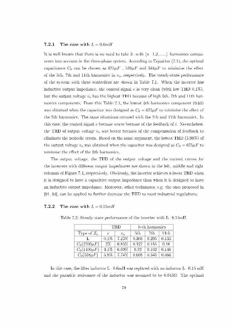
7.2.1 The case with L = 0.6mH
It is well known that there is no need to take 3 · n-th (n=1,2,......) harmonics compo-
nents into account in the three-phase system. According to Equation (7.1), the optimal
capacitance C0 can be chosen as 675µF , 510µF and 344µF to minimise the eect
of the 5th, 7th and 11th harmonics in vo, respectively. The steady-state performance
of the system with these controllers are shown in Table 7.1. When the inverter has
inductive output impedance, the control signal e is very clean (with low THD 0.1%),
but the output voltage vo has the highest THD because of high 5th, 7th and 11th har-
monics components. From this Table 7.1, the lowest 5th harmonics component (0.65)
was obtained when the capacitor was designed as C0 = 675µF to minimise the eect of
the 5th harmonics. The same situations occured with the 7th and 11th harmonics. In
this case, the control signal e became worse because of the feedback of i. Nevertheless,
the THD of output voltage vo was better because of the compensation of feedback to
eliminate the periodic errors. Based on the same argument, the lowest THD (5.98%) of
the output voltage vo was obtained when the capacitor was designed as C0 = 675µF to
minimise the eect of the 5th harmonics.
The output voltage, the THD of the output voltage and the current curves for
the inverters with dierent output impedances are shown in the left, middle and right
columns of Figure 7.4, respectively. Obviously, the inverter achieves a lower THD when
it is designed to have a capacitive output impedance than when it is designed to have
an inductive output impedance. Moreover, other techniques, e.g. the ones proposed in
[91, 92], can be applied to further decrease the THD to meet industrial regulations.
7.2.2 The case with L = 0.15mH
Table 7.2: Steady-state performance of the inverter with L=0.15mH.
THD h-th harmonicsType of Zo e vo 5th 7th 11th
L 0.1% 7.25% 0.306 0.295 0.135C0(2700µF ) 2% 6.85% 0.127 0.185 0.16C0(1400µF ) 4.1% 6.69% 0.32 0.102 0.148C0(558µF ) 5.9% 7.74% 0.605 0.345 0.066
In this case, the lter inductor L=0.6mH was replaced with an inductor L=0.15 mH
and the parasitic resistance of the inductor was assumed to be 0.045Ω. The optimal
70
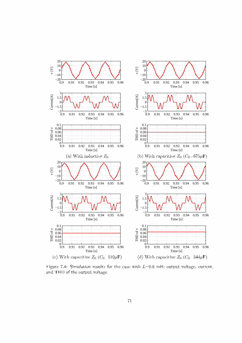
0.9 0.91 0.92 0.93 0.94 0.95 0.96−20−10
01020
v [V
]
Time [s]0.9 0.91 0.92 0.93 0.94 0.95 0.96
−20−10
01020
v [V
]
Time [s]
0.9 0.91 0.92 0.93 0.94 0.95 0.96−3
−1.50
1.53
Cur
rent
[A]
Time [s]0.9 0.91 0.92 0.93 0.94 0.95 0.96
−3−1.5
01.5
3
Cur
rent
[A]
Time [s]
0.9 0.91 0.92 0.93 0.94 0.95 0.960
0.020.040.060.080.1
TH
D o
f v
Time [s]0.9 0.91 0.92 0.93 0.94 0.95 0.960
0.020.040.060.080.1
TH
D o
f v
Time [s]
(a) With inductive Z0 (b) With capacitive Z0 (C0=675µF)
0.9 0.91 0.92 0.93 0.94 0.95 0.96−20−10
01020
v [V
]
Time [s]0.9 0.91 0.92 0.93 0.94 0.95 0.96
−20−10
01020
v [V
]
Time [s]
0.9 0.91 0.92 0.93 0.94 0.95 0.96−3
−1.50
1.53
Cur
rent
[A]
Time [s]0.9 0.91 0.92 0.93 0.94 0.95 0.96
−3−1.5
01.5
3
Cur
rent
[A]
Time [s]
0.9 0.91 0.92 0.93 0.94 0.95 0.960
0.020.040.060.080.1
TH
D o
f v
Time [s]0.9 0.91 0.92 0.93 0.94 0.95 0.960
0.020.040.060.080.1
TH
D o
f v
Time [s]
(c) With capacitive Z0 (C0=510µF) (d) With capacitive Z0 (C0=344µF)
Figure 7.4: Simulation results for the case with L=0.6 mH: output voltage, current,and THD of the output voltage.
71

capacitance C0 can be chosen as 1600µF, 1200µF and 827µF to minimise the eect of
the 5th, 5th+7th and 7th harmonics in vo, respectively. The steady-state performances
of the system with these controllers are shown in Table 7.2. The best THD (16.7%)
was obtained when the capacitor was designed to minimise the eect of the 5th+7th
harmonics as C0=1200µF. The output voltage, the THD of the output voltage and the
current curves for the inverters with dierent output impedances are shown in the left,
middle and right columns of Figure 7.5, respectively.
7.3 Experimental Results
Experiments were also carried out in the stand-alone mode, as shown in Figure 7.6, to
further demonstrate the control strategy. The experimental setup consists of a 42V DC
voltage supply, an inverter board, a LC lter, a board consisting of voltage and current
transducers, a full-bridge rectier loaded with an LC lter L = 150µH, C = 1000µF
and RL = 9Ω, a dSPACE DS1104 R&D controller board with ControlDesk software
and MATLAB Simulink/SimPower software package. The sampling frequency of the
controller was 5 kHz and the switching frequency was 10 kHz. Two cases were tested:
one with L = 0.6 mH and the other with L = 0.15 mH.
7.3.1 The case with L = 0.6mH
The experimental results when the inverter was designed to have dierent types of
output impedance are shown in Figure 7.7. The experimental results are similar to the
simulation ones, but the eect of the THD reduction is not remarkable. However, the
improvement can still be noticed.
7.3.2 The case with L = 0.15mH
The experimental results when the inverter was designed to have dierent types of
output impedance are shown in Figure 7.8. When the inverter was designed to have a
capacitive output impedance to minimise the eect of the 7th harmonics, the best result
was obtained. The THD was improved by about 1% from the case with an inductive
output impedance.
72

0.9 0.91 0.92 0.93 0.94 0.95 0.96−20−10
01020
v [V
]
Time [s]0.9 0.91 0.92 0.93 0.94 0.95 0.96
−20−10
01020
v [V
]
Time [s]
0.9 0.91 0.92 0.93 0.94 0.95 0.96−4−2
024
Cur
rent
[A]
Time [s]0.9 0.91 0.92 0.93 0.94 0.95 0.96
−4−2
024
Cur
rent
[A]
Time [s]
0.9 0.91 0.92 0.93 0.94 0.95 0.960
0.020.040.060.080.1
TH
D o
f v
Time [s]0.9 0.91 0.92 0.93 0.94 0.95 0.960
0.020.040.060.080.1
TH
D o
f v
Time [s]
(a) With inductive Z0 (b) With capacitive Z0 (C0=1600µF)
0.9 0.91 0.92 0.93 0.94 0.95 0.96−20−10
01020
v [V
]
Time [s]0.9 0.91 0.92 0.93 0.94 0.95 0.96
−20−10
01020
v [V
]
Time [s]
0.9 0.91 0.92 0.93 0.94 0.95 0.96−4−2
024
Cur
rent
[A]
Time [s]0.9 0.91 0.92 0.93 0.94 0.95 0.96
−4−2
024
Cur
rent
[A]
Time [s]
0.9 0.91 0.92 0.93 0.94 0.95 0.960
0.020.040.060.080.1
TH
D o
f v
Time [s]0.9 0.91 0.92 0.93 0.94 0.95 0.960
0.020.040.060.080.1
TH
D o
f v
Time [s]
(c) With capacitive Z0 (C0=1200µF) (d) With capacitive Z0 (C0=827µF)
Figure 7.5: Simulation results for the case with L=0.15mH: output voltage, current andTHD of the output voltage.
73

Figure 7.6: The experimental setup
7.4 Conclusions
In this chapter, a synchronverter-based control strategy which introduced a current
feedback was presented to force the output impedance of the inverter to be capacitive.
Both simulation and experimental results were provided to demonstrate that an inverter
achieves a lower THD when it is designed to have a capacitive output impedance than
when it is designed to have an inductive output impedance.
74

0.9 0.91 0.92 0.93 0.94 0.95 0.96−20−10
01020
Vol
tage
[V]
Time [s]0.9 0.91 0.92 0.93 0.94 0.95 0.96
−20−10
01020
Vol
tage
[V]
Time [s]
0.9 0.91 0.92 0.93 0.94 0.95 0.96−3
−1.50
1.53
Cur
rent
[A]
Time [s]0.9 0.91 0.92 0.93 0.94 0.95 0.96
−3−1.5
01.5
3
Cur
rent
[A]
Time [s]
0 0.5 1 1.5 20
0.040.080.120.160.2
TH
D o
f v
Time [s]0 0.5 1 1.5 2
00.040.080.120.160.2
TH
D o
f v
Time [s]
(a) With inductive Z0 (b) With capacitive Z0 (C0=1600µF)
0.9 0.91 0.92 0.93 0.94 0.95 0.96−20−10
01020
Vol
tage
[V]
Time [s]0.9 0.91 0.92 0.93 0.94 0.95 0.96
−20−10
01020
Vol
tage
[V]
Time [s]
0.9 0.91 0.92 0.93 0.94 0.95 0.96−3
−1.50
1.53
Cur
rent
[A]
Time [s]0.9 0.91 0.92 0.93 0.94 0.95 0.96
−3−1.5
01.5
3
Cur
rent
[A]
Time [s]
0 0.5 1 1.5 20
0.040.080.120.160.2
TH
D o
f v
Time [s]0 0.5 1 1.5 2
00.040.080.120.160.2
TH
D o
f v
Time [s]
(c) With capacitive Z0 (C0=1200µF) (d) With capacitive Z0 (C0=827µF)
Figure 7.7: Experimental results for the case with L=0.6mH: output voltage, currentand THD of the output voltage.
75
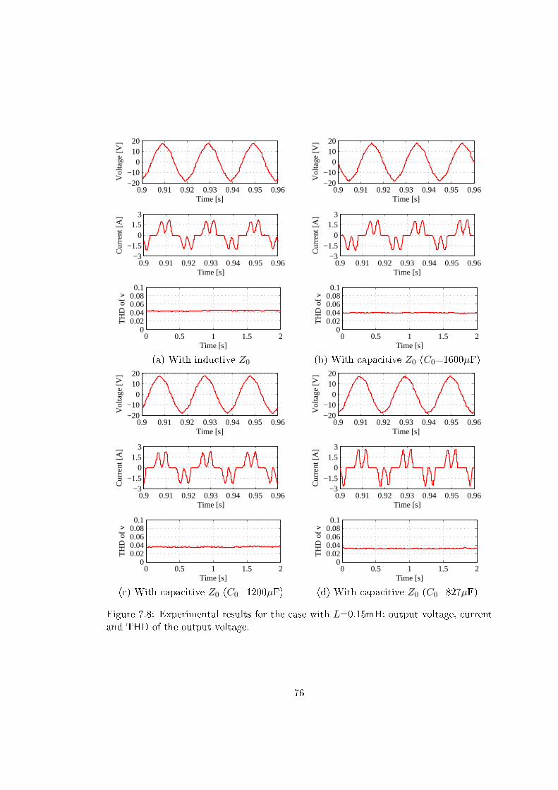
0.9 0.91 0.92 0.93 0.94 0.95 0.96−20−10
01020
Vol
tage
[V]
Time [s]0.9 0.91 0.92 0.93 0.94 0.95 0.96
−20−10
01020
Vol
tage
[V]
Time [s]
0.9 0.91 0.92 0.93 0.94 0.95 0.96−3
−1.50
1.53
Cur
rent
[A]
Time [s]0.9 0.91 0.92 0.93 0.94 0.95 0.96
−3−1.5
01.5
3
Cur
rent
[A]
Time [s]
0 0.5 1 1.5 20
0.020.040.060.080.1
TH
D o
f v
Time [s]0 0.5 1 1.5 2
00.020.040.060.080.1
TH
D o
f v
Time [s]
(a) With inductive Z0 (b) With capacitive Z0 (C0=1600µF)
0.9 0.91 0.92 0.93 0.94 0.95 0.96−20−10
01020
Vol
tage
[V]
Time [s]0.9 0.91 0.92 0.93 0.94 0.95 0.96
−20−10
01020
Vol
tage
[V]
Time [s]
0.9 0.91 0.92 0.93 0.94 0.95 0.96−3
−1.50
1.53
Cur
rent
[A]
Time [s]0.9 0.91 0.92 0.93 0.94 0.95 0.96
−3−1.5
01.5
3
Cur
rent
[A]
Time [s]
0 0.5 1 1.5 20
0.020.040.060.080.1
TH
D o
f v
Time [s]0 0.5 1 1.5 2
00.020.040.060.080.1
TH
D o
f v
Time [s]
(c) With capacitive Z0 (C0=1200µF) (d) With capacitive Z0 (C0=827µF)
Figure 7.8: Experimental results for the case with L=0.15mH: output voltage, currentand THD of the output voltage.
76

Chapter 8
Synchronverters Operated as
Rectiers
Most three-phase rectiers use a diode bridge circuit and a bulk storage capacitor. This
has the advantage of being simple, robust and low cost. However, it allows only undi-
rectional power ow. Moreover, the energy returned from the motor must be dissipated
on the power resistor controlled by a chopper connected across the DC bus. The diode
input circuit also results in a lower power factor and a high level of harmonic input
currents. The voltage source PWM rectier is increasingly used in industrial DC power
supplies, motor drives, and a common DC bus for multiple drives [93]. PWM rectiers
are well known for their advantages and merits compared to uncontrolled diode recti-
ers e.g. lower THD factor, Power Factor correction, regenerative operation and Active
Filtering capabilities [94, 95].
Figure 8.1 presents the most popular topology used in the ASD system for induction
machines, UPS and AC-exited induction generator drive systems utilise the bidirectional
AC-DC-AC power converters. Ls and Rs represent the line impedance. It brings the
current source character of the input circuit and provides the boost feature of converters.
Various strategies have been proposed to control PWM rectiers. These strategies
can achieve the same major goals, such as a high power factor and near-sinusoidal
current waveforms, but they are often based on dierent principles. In particular, the
VOC, which uses closed-loop current control in a rotating reference frame, oers good
dynamic and static performance. It has become very popular and has constantly been
developed and improved [96, 97, 98, 99]. The conguration and performance of the
VOC system largely depends on the quality of the applied current control strategy
77

Q1 Q4
Q3 Q6
va ia Io Q5 Q2
~
~
~
vb vc ib
ic R V o +
-
C
ea eb
ec Rs Ls
Figure 8.1: Representation of three-phase voltage source PWM rectier.
which normally consists of an inner high bandwidth current control loop and an outer
low bandwidth DC bus voltage regulation loop [100]. The current controller controls
the input line current to track the reference to ensure the unity power factor operation
and the power balance on the output of the rectier. The DC bus voltage regulator
indirectly regulates the power fed into the rectier to realise the constant DC bus voltage
control [101, 102, 103].
DPC adopts instantaneous real and reactive power control loops to control the power
directly, without using inner current loops, by using hysteresis control. No PWM block is
needed because the states of the converter switches are selected from a table based on the
instantaneous errors between the set-point and the measured values of real and reactive
power [104, 105, 106, 107, 108, 109]. This leads to a variable switching frequency. It is
dicult to implement in industry because of the variable switching frequency and the
high sampling frequency needed for digital implementation.
In this chapter, two control strategies are proposed to operate a rectier to mimic a
synchronous motor, following the idea of operating inverters to mimic synchronous gen-
erators [1]. This allows the use of a PWM block to convert the voltage into PWM signals
to drive the rectier switches and, hence, the switching frequency is xed. Moreover,
the line currents can be made sinusoidal and good dynamics can be achieved.
8.1 Direct Power Control
The principle of DPC was rst introduced in [104] where an optimum switching table
was dened for the demands of real or reactive power as a function of the power source
78

i Sa Sb Sc
Sq Sp
γψL
Vo
P
Q
Pref
Vref Qref =0 i
p
KK
s+
Switching
Table
Current measurement
&
Power estimator
Figure 8.2: Conventional DPC.
voltage angle. [105] proposed the use of a PWM controlled switched rectier using the
virtual ux signal for power estimation without voltage sensors. Therefore, the most
important thing in this paper is a correct and fast estimation of the real and reactive
power. The real power P and reactive power Q can be dened as
P = Ls(diadt ia + dib
dt ib + dicdt ic) + Vo(Saia + Sbib + Scic),
Q = 1√33Ls(diadt ic −
dicdt ia)− Vo[Sa(ib − ic) + Sb(ic − ia) + Sc(ia − ib),
where ia, ib, ic are three phase line currents; Sa, Sb, Sc are the switching states of the
converter; Vo is the DC bus voltage. The basic block diagram of DPC is shown in
Figure 8.2.
The reference of real power Pref (delivered from the outer PI-DC voltage controller)
and reactive power Qref (set to zero for unity power factor) are compared with the
estimated P and Q values (line voltage or virtual ux), in real and reactive power
hysteresis controllers, respectively.
The digitised output signals of the real and reactive power controllers are dened as
Sp =
1 P < Pref −Hp
0 P > Pref +Hp
,
79

Sq =
1 Q < Qref −Hq
0 Q > Qref +Hq
,
where Hp and Hq are the hysteresis bands.
The digitised variables Sp, Sq and the ux vector position γψL = arctan(ψLαψLβ)γψL,
which, by accessing the address of the look-up table, select the appropriate voltage
vector according to the switching table[104].
The region of the voltage or ux vector position is divided into twelve sectors and
the sectors can be numerically expressed as
(n− 2)π
6≤ γ ≤ (n− 1)π
6,
where, n=1,2,. . . ,12.
However, superimpositions of the disturbances on the line voltage have direct inu-
ences on the line voltage vector position in the control system. Sometimes, this kind of
problem can be overcome by phase-locked loops only, but the quality of the controlled
system depends on the eectiveness of PLL design.
8.2 Modeling of a Synchronous Motor
A three-phase PWM bridge rectier is shown in Figure 8.3. Inductors Ls with equivalent
series resistance Rs are connected between the rectier and the source to reduce the
current harmonics. Assume that the eld and the three identical stator windings are
distributed in slots around the periphery of the uniform air gap. The stator windings
can be regarded as concentrated coils having self-inductance L and mutual inductance
−M (M > 0, the negative sign is due to the 2π3 phase angle). In this chapter, the model
of a synchronous motor presented in [1] is adopted because the model for a generator
or a motor is more or less the same, apart from the direction of the stator current is
dened as opposite.
Denote the ux vector and the current vector as
Φ =
Φa
Φb
Φc
, i =
ia
ib
ic
respectively, and
80
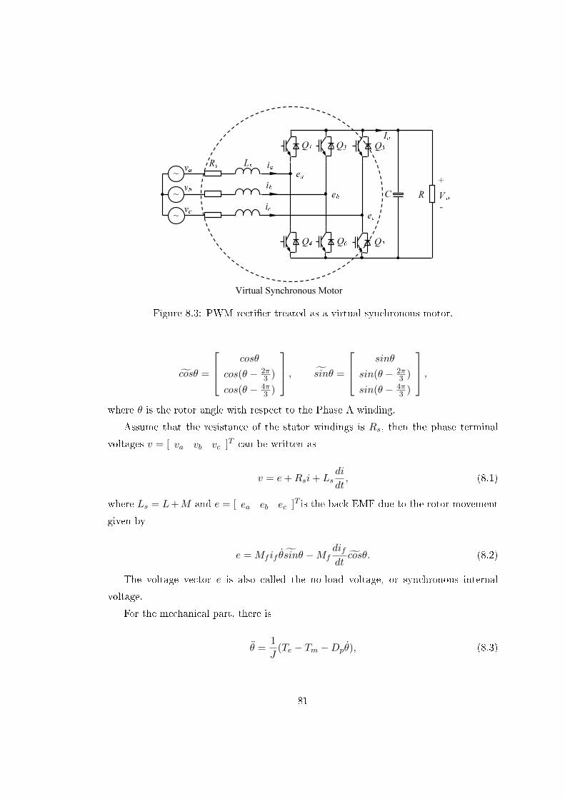
Q1 Q4
Q3 Q6
va ia Io Q5 Q2
~
~
~
vb vc ib
ic R V o +
-
C
ea eb
ec Virtual Synchronous Motor
Rs Ls
Figure 8.3: PWM rectier treated as a virtual synchronous motor.
cosθ =
cosθ
cos(θ − 2π3 )
cos(θ − 4π3 )
, sinθ =
sinθ
sin(θ − 2π3 )
sin(θ − 4π3 )
,where θ is the rotor angle with respect to the Phase A winding.
Assume that the resistance of the stator windings is Rs, then the phase terminal
voltages v = [ va vb vc ]T can be written as
v = e+Rsi+ Lsdi
dt, (8.1)
where Ls = L+M and e = [ ea eb ec ]T is the back EMF due to the rotor movement
given by
e = Mf if θsinθ −Mfdifdtcosθ. (8.2)
The voltage vector e is also called the no-load voltage, or synchronous internal
voltage.
For the mechanical part, there is
θ =1
J(Te − Tm −Dpθ), (8.3)
81

a-axis Rotor field axis θ sR , sL ai
av fR , fL M
Field voltage fv fi
bv cv
bi ci b-axis c-axis
Figure 8.4: Structure of an idealized three-phase round-rotor synchronous motor.
where J is the moment of inertia of all the parts rotating with the rotor; Dp is a damping
factor; Tm is the mechanical torque and Te is the electromagnetic torque
Te = Mf if
⟨i, sinθ
⟩, (8.4)
where 〈·, ·〉 denotes the conventional inner product in R3.
Dene the generated real power P and reactive power Q as
P = vaia + vbib + vcic, (8.5)
Q =1√3
[(vb − vc)ia + (vc − va)ib + (va − vb)ic]. (8.6)
The model can be described with the block diagram shown in Figure 8.5. Thus, the
state variables of the synchronous motor are i (the inductor currents), θ and θ (which
82

Tm θɺ θ Te P
Q e v f fM i i
1Js 1 1s 1s sR L s+
Dp Eqn.(8.2) Eqn.(8.4) Eqn.(8.5) Eqn.(8.6)
Figure 8.5: The model of a synchronous motor.
are a virtual angle and a virtual angular speed). Tm and Mf if are the control inputs
of the synchronous motor. The control strategy will be discussed in the next section.
8.3 Proposed Strategy
The STA, which is the basic component of the proposed controller for synchronisation,
is explained in subsection A. The proposed methodology of DPC, which is based on
the virtual synchronous motor, is explained in subsection B. The proposed strategy to
control the output voltage is described in subsection C and some applications are given
in subsection D.
8.3.1 STA
In order for the strategy to work properly, the frequency θ inside the rectier should
be the same as, or very close to the grid frequency θg. Before the rectier is connected
to the power source, its phase θ should be kept the same as that of the grid in order
to minimise the settling time when connecting it to the grid. This can be achieved by
measuring the phase of the grid, e.g. via a phase-locked loop. In this control strategy,
STA [110] is adopted to generate a signal to reset the integrator and the grid frequency.
A nonstationary sinusoidal y(t) can be expressed as
y(t) = A(t)sin(∫ tω(τ)dτ + δ(t)),
83
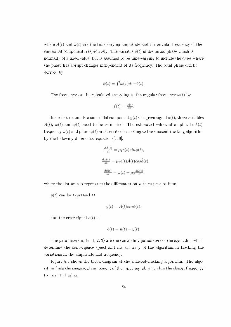
where A(t) and ω(t) are the time-varying amplitude and the angular frequency of the
sinusoidal component, respectively. The variable δ(t) is the initial phase which is
normally of a xed value, but is assumed to be time-varying to include the cases where
the phase has abrupt changes independent of its frequency. The total phase can be
derived by
φ(t) =∫ tω(τ)dτ+δ(t).
The frequency can be calculated according to the angular frequency ω(t) by
f(t) = ω(t)2π .
In order to estimate a sinusoidal component y(t) of a given signal u(t), three variables
A(t), ω(t) and φ(t) need to be estimated. The estimated values of amplitude A(t),
frequency ω(t) and phase φ(t) are described according to the sinusoid-tracking algorithm
by the following dierential equations[110]:
dA(t)dt = µ1e(t)sinφ(t),
dω(t)dt = µ2e(t)A(t)cosφ(t),
dφ(t)dt = ω(t) + µ3
dω(t)dt ,
where the dot on top represents the dierentiation with respect to time.
y(t) can be expressed as
y(t) = A(t)sinφ(t),
and the error signal e(t) is
e(t) = u(t)− y(t).
The parameters µi (i=1, 2, 3) are the controlling parameters of the algorithm which
determine the convergence speed and the accuracy of the algorithm in tracking the
variations in the amplitude and frequency.
Figure 8.6 shows the block diagram of the sinusoid-tracking algorithm. The algo-
rithm nds the sinusoidal component of the input signal, which has the closest frequency
to its initial value.
84
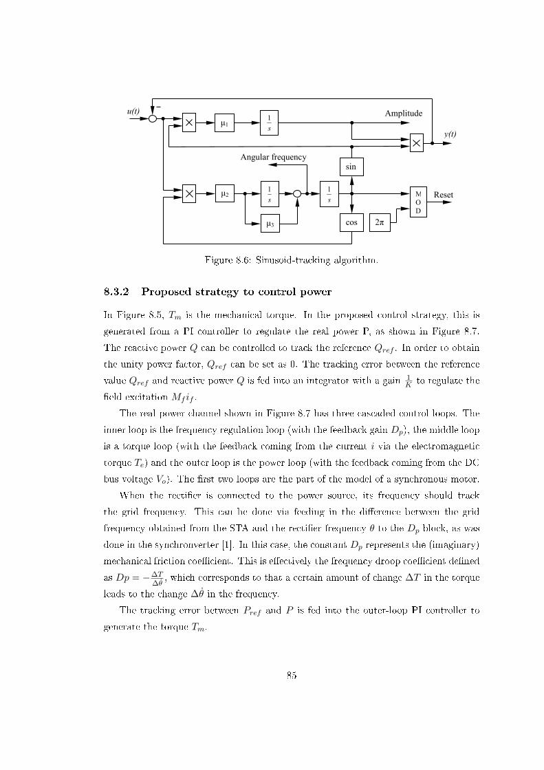
u(t)
µ1
µ2
µ3
sin
cos
2π
M
O
D
y(t)
Amplitude
Reset
Angular frequency
1
s
1
s
1
s
Figure 8.6: Sinusoid-tracking algorithm.
8.3.2 Proposed strategy to control power
In Figure 8.5, Tm is the mechanical torque. In the proposed control strategy, this is
generated from a PI controller to regulate the real power P, as shown in Figure 8.7.
The reactive power Q can be controlled to track the reference Qref . In order to obtain
the unity power factor, Qref can be set as 0. The tracking error between the reference
value Qref and reactive power Q is fed into an integrator with a gain 1K to regulate the
eld excitation Mf if .
The real power channel shown in Figure 8.7 has three cascaded control loops. The
inner loop is the frequency regulation loop (with the feedback gain Dp), the middle loop
is a torque loop (with the feedback coming from the current i via the electromagnetic
torque Te) and the outer loop is the power loop (with the feedback coming from the DC
bus voltage Vo). The rst two loops are the part of the model of a synchronous motor.
When the rectier is connected to the power source, its frequency should track
the grid frequency. This can be done via feeding in the dierence between the grid
frequency obtained from the STA and the rectier frequency θ to the Dp block, as was
done in the synchronverter [1]. In this case, the constant Dp represents the (imaginary)
mechanical friction coecient. This is eectively the frequency droop coecient dened
as Dp = −∆T∆θ
, which corresponds to that a certain amount of change ∆T in the torque
leads to the change ∆θ in the frequency.
The tracking error between Pref and P is fed into the outer-loop PI controller to
generate the torque Tm.
85
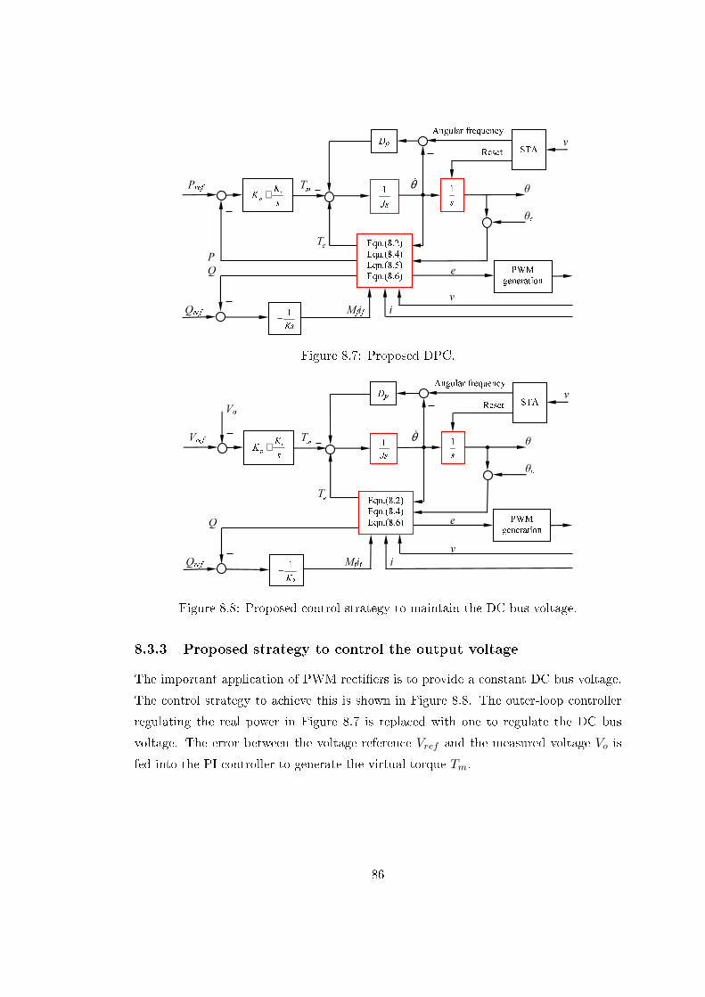
Pref mT θɺ eT P
Q e v
Qref Mfif i
1JsDp
1Ks−
ip KK s+ 1s STA θ
θc v Reset Angular frequency
PWM generation Eqn.(8.2) Eqn.(8.4) Eqn.(8.5) Eqn.(8.6) Figure 8.7: Proposed DPC.
Vo
Vref mT θɺ eT
Q v
Qref Mfif i
1Js 1s Dp
1Ks−
PWM generation STA ip KK s+
e
θ
θc v Reset Angular frequency
Eqn.(8.2) Eqn.(8.4) Eqn.(8.6) Figure 8.8: Proposed control strategy to maintain the DC bus voltage.
8.3.3 Proposed strategy to control the output voltage
The important application of PWM rectiers is to provide a constant DC bus voltage.
The control strategy to achieve this is shown in Figure 8.8. The outer-loop controller
regulating the real power in Figure 8.7 is replaced with one to regulate the DC bus
voltage. The error between the voltage reference Vref and the measured voltage Vo is
fed into the PI controller to generate the virtual torque Tm.
86
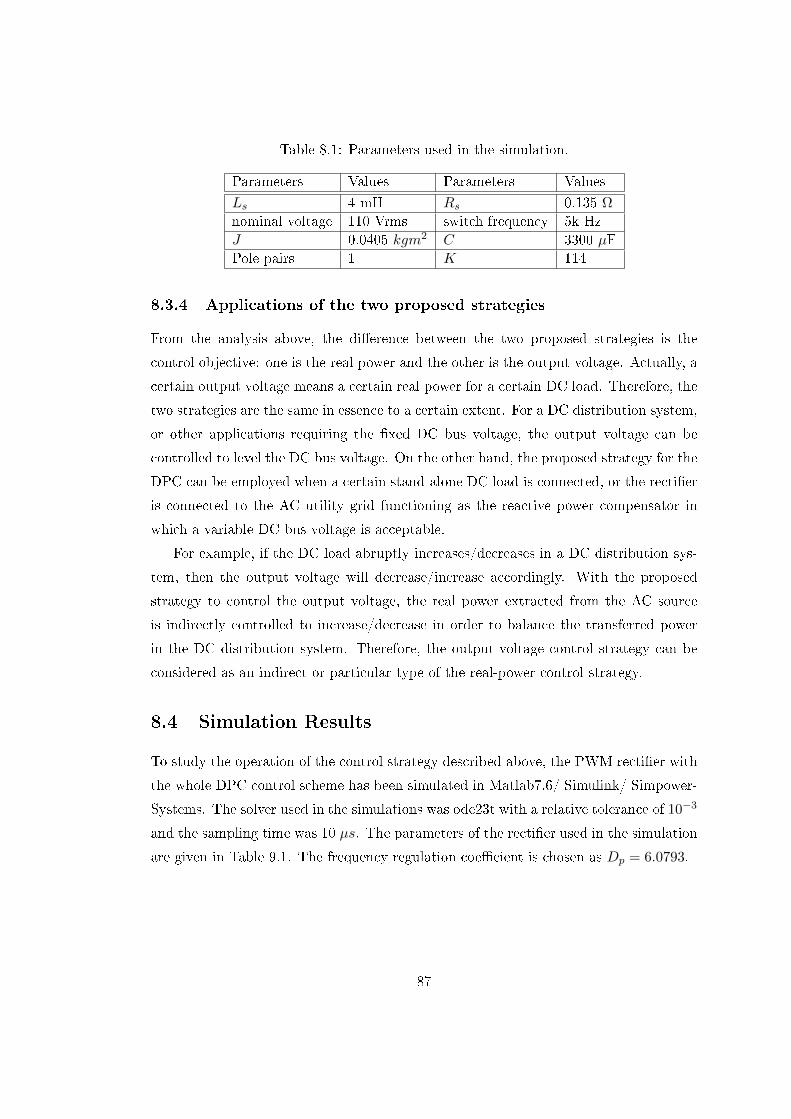
Table 8.1: Parameters used in the simulation.
Parameters Values Parameters ValuesLs 4 mH Rs 0.135 Ω
nominal voltage 110 Vrms switch frequency 5k HzJ 0.0405 kgm2 C 3300 µFPole pairs 1 K 114
8.3.4 Applications of the two proposed strategies
From the analysis above, the dierence between the two proposed strategies is the
control objective: one is the real power and the other is the output voltage. Actually, a
certain output voltage means a certain real power for a certain DC load. Therefore, the
two strategies are the same in essence to a certain extent. For a DC distribution system,
or other applications requiring the xed DC bus voltage, the output voltage can be
controlled to level the DC bus voltage. On the other hand, the proposed strategy for the
DPC can be employed when a certain stand-alone DC load is connected, or the rectier
is connected to the AC utility grid functioning as the reactive power compensator in
which a variable DC bus voltage is acceptable.
For example, if the DC load abruptly increases/decreases in a DC distribution sys-
tem, then the output voltage will decrease/increase accordingly. With the proposed
strategy to control the output voltage, the real power extracted from the AC source
is indirectly controlled to increase/decrease in order to balance the transferred power
in the DC distribution system. Therefore, the output-voltage control strategy can be
considered as an indirect or particular type of the real-power control strategy.
8.4 Simulation Results
To study the operation of the control strategy described above, the PWM rectier with
the whole DPC control scheme has been simulated in Matlab7.6/ Simulink/ Simpower-
Systems. The solver used in the simulations was ode23t with a relative tolerance of 10−3
and the sampling time was 10 µs. The parameters of the rectier used in the simulation
are given in Table 9.1. The frequency regulation coecient is chosen as Dp = 6.0793.
87

0 1 2 3 4 5300305310315320325330
Time [s]
Spee
d [r
ad/s
]
θg θ
0 1 2 3 4 50
102030405060
Vol
tage
[V
]
Time [s]
(a) Virtual speed and grid speed (b) DC bus voltage (V)
0 1 2 3 4 50
20
40
60
80
100
Time [s]
P [W
]
P
ref P
0 1 2 3 4 5−100
−50
0
50
100
Time [s]
Q [V
ar]
Q
ref Q
(c) P (W) (d) Q (Var)
0.1 0.15 0.2 0.25 0.3−20
−10
0
10
20
30
Time [s]
[V/A
]
va
ia
2.5 2.55 2.6 2.65 2.7−20
−10
0
10
20
30
Time [s]
[V/A
]
va
ia
(e) Voltage and current (uncontrollable) (f) Voltage and current (PWM)
Figure 8.9: Simulation results with the nominal grid frequency.
8.4.1 DPC
The simulation was started at t = 0. An STA was used for the initial synchronisation at
the rst 0.5 second. During this time, the PWM rectier worked as an uncontrollable
rectier. The reactive power reference Qref was set to zero to obtain the unity power
factor. Initially, the real power reference Pref was 30W and the load R was 50Ω. The
real power reference was increased to Pref = 50W at t = 2s and the load was changed
to R = 30Ω at t = 3.5s. In this simulation, Kp = 0.05 and Ki = 0.5 are proportional
and integral gains for a PI controller of the real power loop, respectively.
The system responses are shown in Figure 8.9. The virtual angular speed θ tracked
the grid angular speed θg very well before the connection. There were small transient
responses at the connection time, but they quickly settled down after the connection.
88

0 1 2 3 4 5300305310315320325330
Time [s]
Spee
d [r
ad/s
]
θg θ
0 1 2 3 4 50
1020304050607080
Time [s]
Vol
tage
[V
]
V
refV
o
(a) Virtual speed and grid speed (b) Vref and Vo (V)
0 1 2 3 4 50
20
40
60
80
100
P [k
W]
Time [s]0 1 2 3 4 5
−100
−50
0
50
100
Time [s]
Q [k
Var
]
Q
ref Q
(c) Real power (W) (d) Reactive power (Var)
0.1 0.15 0.2 0.25 0.3−20
−10
0
10
20
30
Time [s]
[V/A
]
va
ia
2.5 2.55 2.6 2.65 2.7−20
−10
0
10
20
30
Time [s]
[V/A
]
va
ia
(e) Voltage and current (uncontrollable) (d) Voltage and current (PWM)
Figure 8.10: Simulation results when maintaining DC bus voltage.
The real power changed slightly but quickly recovered to the reference value. Meanwhile,
the DC bus voltage changed gradually because of the capacitor on the DC bus. The
reactive power was maintained at zero, apart from when there were changes in the
reference or the load. The input voltage and current were in the same phase, which
means the unity power factor is always achieved.
8.4.2 Regulation of the output voltage
The reactive power reference Qref was set to zero for the unity power factor and the
output voltage reference Vref was set at 40V. The load R was 50Ω at the beginning.
The output voltage reference was changed to Vref = 50V at t = 2s and the load was
changed to R = 30Ω at t = 3.5s. In this simulation, Kp = 0.02 and Ki = 0.2 are
89

Q1 Q4
Q3 Q6
va ia Io Q5 Q2
vb vc ib
ic R V o +
-
C
ea eb
ec Ls Rs Relay
RL Transformer
230/12 Grid
Figure 8.11: Experimental topology.
proportional and integral gains for a PI controller of the voltage loop, respectively.
The system responses are shown in the Figure 8.10. The virtual angular speed θ
tracked the grid angular speed θg very well all the time. The results are similar to the
previous case. There was a big overshoot on the real power when the DC bus voltage
reference changed due to the eect of the DC bus capacitor. The output voltage tracked
the reference voltage very well. When the load was changed, the voltage dropped but
quickly returned to the reference value.
8.5 Experiment Results
Experiments were also carried out on a test rig, of which the parameters are roughly
the same as those given in Table 9.1 and the control parameters are the same, to further
demonstrate the analysis. The experimental setup consists of a rectier board, a three-
phase grid interface inductor, a board consisting of voltage and current transducers, a
step-up transformer, a dSPACE DS1104 R&D controller board with ControlDesk soft-
ware and the MATLAB Simulink/SimPower software package. The sampling frequency
of the controller is 5kHz and the switching frequency is 10 kHz. For safety reasons,
this test rig was a low-power low-voltage system but it was enough to demonstrate the
proposed strategy and to compare the results with the simulation results. The parame-
ters used in the experimental setup are the same as those used in the simulations given
in Table 9.1. The experimental topology is shown in Figure 9.8 and the experimental
setup is shown in Figure 8.12.
90

Figure 8.12: Experimental setup.
8.5.1 DPC
The experiment was carried out according to the following sequence of actions:
1) start the system, but keep all the IGBTs o; use the STA algorithm to synchronise
the grid's frequency;
2) turn the relay on roughly at t=3s;
3) connect to the load R=50Ω roughly at t=5s;
4) start operating the IGBTs roughly at t=10s, Pref=40W and Q loop was closed;
5) activate the Q loop roughly at t=20s;
6) apply Pref=60W roughly at t=30s;
7) change the load to R=30Ω roughly at t=41s.
Figure 8.13 shows the responses of the system. θ tracked θg very well all the time.
From the beginning to 3s, most of the power is lost on RL which makes the system safe
for building up DC bus voltage slowly at the beginning. The DC bus voltage was built
up at around 26V. The real power and reactive power were zero because there was no
load on the DC bus. In order to remove RL, relays were turned on at t=3s. The real
power, increased slightly for charging the DC bus capacitor, then went back to zero, so
that the the DC bus voltage went up to 28V. When the load R=50Ω was connected to
DC bus at t=5s, the real power increased to 16W. Theoretically, the DC bus voltage
91
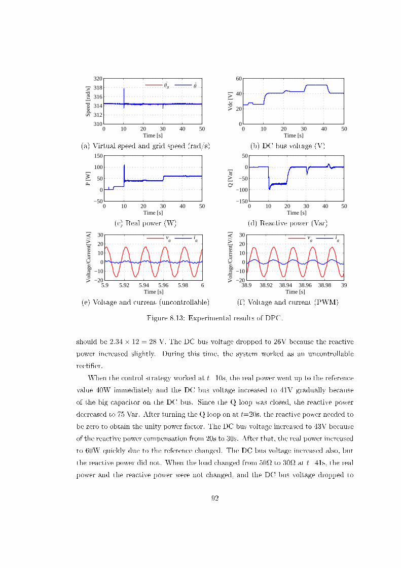
0 10 20 30 40 50310
312
314
316
318
320
Time [s]
Spee
d [r
ad/s
]
θg θ
0 10 20 30 40 500
20
40
60
Vdc
[V
]
Time [s]
(a) Virtual speed and grid speed (rad/s) (b) DC bus voltage (V)
0 10 20 30 40 50−50
0
50
100
150
P [W
]
Time [s]0 10 20 30 40 50
−150
−100
−50
0
50
Q [V
ar]
Time [s]
(c) Real power (W) (d) Reactive power (Var)
5.9 5.92 5.94 5.96 5.98 6−20
−10
0
10
20
30
Time [s]
Vol
tage
/Cur
rent
[V/A
]
va
ia
38.9 38.92 38.94 38.96 38.98 39−20
−10
0
10
20
30
Time [s]
Vol
tage
/Cur
rent
[V/A
]
va
ia
(e) Voltage and current (uncontrollable) (f) Voltage and current (PWM)
Figure 8.13: Experimental results of DPC.
should be 2.34× 12 = 28 V. The DC bus voltage dropped to 26V because the reactive
power increased slightly. During this time, the system worked as an uncontrollable
rectier.
When the control strategy worked at t=10s, the real power went up to the reference
value 40W immediately and the DC bus voltage increased to 41V gradually because
of the big capacitor on the DC bus. Since the Q loop was closed, the reactive power
decreased to 75 Var. After turning the Q loop on at t=20s, the reactive power needed to
be zero to obtain the unity power factor. The DC bus voltage increased to 43V because
of the reactive power compensation from 20s to 30s. After that, the real power increased
to 60W quickly due to the reference changed. The DC bus voltage increased also, but
the reactive power did not. When the load changed from 50Ω to 30Ω at t=41s, the real
power and the reactive power were not changed, and the DC bus voltage dropped to
92
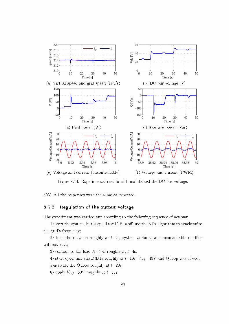
0 10 20 30 40 50310
312
314
316
318
320
Time [s]
Spee
d [r
ad/s
]
θg θ
0 10 20 30 40 500
20
40
60
Vdc
[V
]
Time [s]
(a) Virtual speed and grid speed (rad/s) (b) DC bus voltage (V)
0 10 20 30 40 50−50
0
50
100
150
P [W
]
Time [s]0 10 20 30 40 50
−150
−100
−50
0
50
Q [V
ar]
Time [s]
(c) Real power (W) (d) Reactive power (Var)
5.9 5.92 5.94 5.96 5.98 6−20
−10
0
10
20
30
Time [s]
Vol
tage
/Cur
rent
[V/A
]
va
ia
38.9 38.92 38.94 38.96 38.98 39−20
−10
0
10
20
30
Time [s]
Vol
tage
/Cur
rent
[V/A
]
va
ia
(e) Voltage and current (uncontrollable) (f) Voltage and current (PWM)
Figure 8.14: Experimental results with maintained the DC bus voltage.
40V. All the responses were the same as expected.
8.5.2 Regulation of the output voltage
The experiment was carried out according to the following sequence of actions:
1) start the system, but keep all the IGBTs o; use the STA algorithm to synchronise
the grid's frequency;
2) turn the relay on roughly at t=2s, system works as an uncontrollable rectier
without load;
3) connect to the load R=50Ω roughly at t=4s;
4) start operating the IGBTs roughly at t=10s, Vref=40V and Q loop was closed;
5)activate the Q loop roughly at t=20s;
6) apply Vref=50V roughly at t=30s;
93

7) change the load to R=30Ω roughly at t=41s..
Figure 8.14 shows the responses of the system. From t=0 to 10s, the results are
totally the same as the previous case. When the control strategy worked at t=10s,
the DC bus voltage increased to the reference value 40V and the real power increased
to around 40W. Since the Q loop was closed, the reactive power decreased to 70Var.
After turning the Q loop on at t=20s, the reactive power needed to be zero to obtain
the unity power factor. The real power dropped slightly because of the reactive power
compensation from 20s to 30s. The DC bus voltage kept the reference value very well.
After this, the DC bus voltage increased to 50V quickly due to the reference change.
The real power increased as well but the reactive power did not. When the load changed
from 50Ω to 30Ω at t=41s, the DC bus voltage and the reactive power did not change,
and the real power went up to 95W.
8.6 Conclusions
In this chapter, the three-phase PWM rectiers are operated to mimic a synchronous
motor with two dierent control strategies, which can possess most of the characteristics
of conventional synchronous motors. Therefore, when PWM rectiers are connected
with the utility grid, the previous operation methods of the utility grid can still be
used regardless of the particular load characteristics; the stability of the utility grid can
be improved accordingly. In the proposed schemes, the real power extracted from the
source and the output voltage are the control objectives, respectively, hence they can be
employed in dierent applications. Moreover, the reactive power can easily be controlled
to remain at zero in the steady state so that the unity power factor is obtained. Both
simulation and experimental results are provided to demonstrate the proposed control
strategies.
94

Chapter 9
Synchronverters Operated as
Rectiers without a PLL
PWM-controlled rectiers are increasingly used in industrial applications, such as ASD
for induction machines and UPS, with bidirectional AC-DC-AC power converters. When
compared with conventional diode rectiers, PWM-controlled rectiers have many ad-
vantages such as output voltage control, direct power control, sinusoidal line current
with low THD, power factor correction, and bi-directional power ow [94, 95].
Various control strategies have been proposed in recent years for PWM-controlled
rectiers. The classical solution is the VOC scheme, which uses closed-loop current
control in the rotating reference frame. It oers good dynamic and static performance
and has constantly been developed and improved [96, 97, 98, 99]. The conguration
and performance of a VOC system largely depend on the quality of the applied current
control strategy, which normally consists of an inner high bandwidth current control loop
and an outer low bandwidth DC voltage regulation loop [100]. The current controller
regulates the line current to track the reference to ensure unity power factor operation
and power balance on the output of the rectier. The DC bus voltage regulator indirectly
regulates the power fed into the rectier to achieve constant DC bus voltage control
[101, 102, 103].
Another solution is based on the idea of DPC. It adopts instantaneous real and re-
active power control loops to control the power directly using hysteresis control, without
using inner current loops. No pulse-width-modulation (PWM) block is needed because
the states of the converter switches are selected from a table based on the instantan-
eous errors between the set-point and the measured values of real and reactive power
95

Q1 Q4
Q3 Q6
va ia Io Q5 Q2
~
~
~
vb vc ib
ic R V o +
-
C
ea eb
ec Rs Ls
Figure 9.1: A three-phase PWM-controlled rectier.
[104, 105, 106, 107, 108, 109]. This leads to a variable switching frequency. It is di-
cult to implement in industry because of the variable switching frequency and the high
sampling frequency needed for digital implementation.
Recently, the synchronverter technology [40, 1] has been proposed as an inverter to
mimic synchronous generators and, hence, it considerably facilitates the grid connection
of renewable energy and smart grid integration. Since synchronous generators have been
studied for more than 100 years, and the relevant technologies have reached a high level
of maturity, all these technologies can easily be applied to control inverters. Moreover,
the synchronverter technology has been extended to operate a rectier to mimic SM
[111]. This strategy can control the output voltage and the power directly with excellent
performance.
It has become a convention for control strategies of a grid-connected converter (in-
verter or rectier), regardless of the methods applied, to embed a synchronisation unit,
e.g. a PLL [112, 113], to provide the information about the grid frequency and phase so
that the converter is able to synchronise with the grid voltage. As a result, a large num-
ber of research activities have been developed for PLL [114, 115, 116, 117, 118, 119, 120].
It is known that PLLs have a negative impact on control performance [121, 122] and
it is benecial if it can be removed. A slow PLL could directly aect the control per-
formance and degrade system stability but a complex PLL, on the other hand, is often
computationally intensive, which adds signicant burden to the controller.
In this chapter, a control strategy is presented to control the output voltage for three-
phase PWM-controlled rectiers. The controller is able to track the grid frequency and
phase automatically so that an extra synchronisation unit is no longer needed. This
96

mT
eT
Q Mfif
1Js 1s e
θ
θc ip KK s+
ifpf KK s+
1s sL R+
nθɺ
gθ∆ ɺ
T∆
rθɺ
i
v
v 1 2 is S 1Ks−
θɺ
ivpv KK s+ Eqn.(8.2) Eqn.(8.4) Eqn.(8.5) Qref Vref Vo θ∆ ɺ
Figure 9.2: Control strategy to regulate the output voltage.
not only improves the performance of the system but also considerably reduces the
complexity of the overall controller.
9.1 Proposed Control Strategies
9.1.1 Regulation of the output voltage
The proposed controller to regulate the output voltage of a PWM-controlled rectier is
shown in Figure 9.2. Comparing this to Figure 8.8, it is easy to see that there are three
major changes. Firstly, a virtual current is generated from the error between the grid
voltage v and the control signal e is introduced, and the current fed into the controller
can be either the virtual current is or the grid current i. Secondly, the synchronisation
unit, which provides the grid frequency reference and the reset signal, is removed from
the controller. Finally, a PI controller is added to generate the reference speed θr for the
virtual synchronous motor, while driving the error between the reference speed θr and
the virtual speed θ to zero. It will be shown later that the reference speed θr converges
to the grid frequency at the steady state.
It is well known that a three-phase PWM-controlled rectier consists of six switches
with anti-parallelled diodes, as shown in Figure 9.1. When all the switches are o,
the three-phase PWM-controlled rectier works as an uncontrolled rectier which only
consists of six diodes. Analyses are given below for both the uncontrolled mode and the
97
PWM-controlled mode to explain how the controller works and why the changes should
be made.
9.1.1.1 Uncontrolled mode
When turning on the switches, the control signals e must be synchronised with the
grid voltage v, with the same phase sequence. Otherwise, high inrush currents may
ow through the line impedance from the grid to the rectier because of the error
between the control signals e and the grid voltage v, which might destroy the relevant
components in the circuit. Moreover, it would be ideal if the amplitude E is also the
same as the amplitude of v.
During the uncontrolled mode, the Q-loop of the controller and the DC bus voltage
loop should be disabled. The virtual mechanical torque Tm can be set to be zero and the
virtual eld excitation Mf if can be set as Eθn, where θn is the nominal grid frequency
(here θn = 100π). However, the current i owing through the line impedance from the
grid to the rectier is not available for the controller because the current i cannot be
controlled by the controller when the rectier is operated in the uncontrolled mode. In
order to solve this problem, a virtual current
is =1
sLs +Rs(v − e), (9.1)
which is generated from the error between v and e, is introduced to replace i for feedback
so that Te can be calculated according to Equation (8.4). Since the current is is not
physical, the virtual synchronous inductor sLs + Rs can be small to speed up the
synchronisation process.
When the control signal e is equal to the grid voltage v, the virtual current is is zero
according to Equation (9.1), so that the controller is synchronised with the grid. After
synchronisation, the switches can be turned on at any time to operate the rectier in the
PWM-controlled mode. At the same time, the Switch S should be turned to Position 2
so that the real current i is fed into the controller for the normal operation. Note that
although the control signal e is the same as the grid voltage v, the recovered voltage
at the terminals of the PWM-controlled rectier is in phase with v but with a smaller
amplitude because the DC bus voltage is not high enough. Hence, the inrush current
when turning the switches on can only be reduced, but not completely eliminated.
98

9.1.1.2 PWM-controlled mode
When the rectier is operated in the PWM-controlled mode, not only should the Switch
S be turned to Position 2, but also the Q-loop and the DC bus voltage loop should be
enabled at the same time. Since the regulation of the output voltage and the reactive
power are outlined in the last section, only the characteristics that are dierent from
the control strategy are described here.
It is well known that the phase dierence
δ = θg − θ (9.2)
where θg is the phase of the grid voltage. The phase dierence is often called the
power angle and is controlled by the virtual mechanical torque Tm. If the grid phase
θg (or speed θg) decreases, then the power angle δ decreases according to Equation
(9.2). As a result, the real power fed into the rectier decreases and the output voltage
of the rectier also decreases when the load is not changed. This causes the virtual
mechanical torque Tm to increase because of the regulation of the DC bus voltage PI
controller (Kpv + Kivs ). As a result, the input to the integrator block 1
Js in Figure 9.2
decreases, because of the negative sign before the summation block, and the speed θ of
the virtual SM decreases. At the same time, ∆θ increases so that ∆θg also increases
because of the regulation of the frequency PI controller (Kpf +Kifs ), which causes the
speed reference θr to decrease according to θr = θn − ∆θg. The regulation process
continues till θ = θr and θr = θg.
If the grid frequency θg increases, then a similar process happens till θ = θr = θg.
Therefore, the frequency θ is able to track the grid frequency θg automatically so that
the controller does not need an extra synchronisation unit to provide the grid frequency
θg as the reference frequency.
9.1.2 Regulation of the power
Direct Power Control (DPC) adopts instantaneous real and reactive power control loops
to control the power directly. The control strategy to achieve this is shown in Figure
9.3. The outer-loop controller regulating the output voltage in Figure 9.2 is replaced
with one to regulate the real power. The error between the real power reference Prefand the real power P is fed into the real power PI controller (Kpp +
KipS ) to generate
99
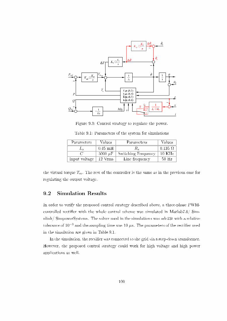
mT
eT
Mfif
1Js 1s e
θ
θc ip KK s+
ifpf KK s+
1s sL R+
nθɺ
gθ∆ ɺ
T∆
rθɺ
i
v
v 1 2 is S 1Ks−
θɺ
ippp KK s+ Eqn.(8.2) Eqn.(8.4) Eqn.(8.5) Eqn.(8.6) Qref Pref
P
Q
θ∆ ɺ
Figure 9.3: Control strategy to regulate the power.
Table 9.1: Parameters of the system for simulations
Parameters Values Parameters ValuesLs 0.45 mH Rs 0.135 Ω
C 5000 µF Switching Frequency 10 KHzInput voltage 12 Vrms Line frequency 50 Hz
the virtual torque Tm. The rest of the controller is the same as in the previous case for
regulating the output voltage.
9.2 Simulation Results
In order to verify the proposed control strategy described above, a three-phase PWM-
controlled rectier with the whole control scheme was simulated in Matlab7.6/ Sim-
ulink/ SimpowerSystems. The solver used in the simulations was ode23t with a relative
tolerance of 10−3 and the sampling time was 10 µs. The parameters of the rectier used
in the simulation are given in Table 9.1.
In the simulation, the rectier was connected to the grid via a step-down transformer.
However, the proposed control strategy could work for high voltage and high power
applications as well.
100

Table 9.2: Parameters of the controller.
Parameters Values Parameters ValuesKpf 0.5 Kif 7Kpv 0.01 Kiv 0.1J 0.0002 kgm2 K 370
0 1 2 3 4 5 6 7 8313
313.5
314
314.5
315
315.5
316
Time [s]
Freq
uenc
y [r
ad/s
]
θg θ
0 1 2 3 4 5 6 7 80
1020304050607080
Time [s]
Vol
tage
[V
]
V
refV
o
(a) Frequency (rad/s) (b) DC bus voltage (V)
0 1 2 3 4 5 6 7 80
20406080
100120140
P [W
]
Time [s]0 1 2 3 4 5 6 7 8
−100−75−50−25
0255075
100
Time [s]
Q [V
ar]
Q
ref Q
(c) Real power (W) (d) Reactive power (Var)
Figure 9.4: Simulation results when regulating the output voltage.
9.2.1 Regulation of the output voltage
The parameters of the controller used in the simulation are shown in Table 9.2.
The simulation was started at t = 0 s, with Switch S at Position 1. The rectier
worked in the uncontrolled mode for the rst 0.5 s, during which the DC bus voltage
loop and the Q-loop were disabled in order for the rectier to synchronise with the
grid voltage. At t = 0.5 s, the DC bus voltage loop and the Q-loop were enabled, the
Switch S was switched to Position 2 and the PWM signals were released to the rectier.
Initially, the output voltage reference Vref was 40 V and the reactive power reference
Qref was set to zero to obtain the unity power factor for a load R of 50 Ω. The output
voltage reference was increased to Vref = 50 V at t = 2 s and the load was changed to
R = 25 Ω at t = 3.5 s. At t = 5 s, the grid voltage frequency decreased from 50 Hz to
49.95 Hz and at t = 6.5 s the reactive power reference was changed to Qref = 30 Var .
101

0.3 0.34 0.38 0.42 0.46 0.5−20
−10
0
10
20
30
Time [s]
v a and
e a
v
ae
a
4.8 4.84 4.88 4.92 4.96 5−20
−10
0
10
20
30
Time [s]
v a and
e a
v
ae
a
(a) In the uncontrolled mode (b) In the PWM-controlled mode
Figure 9.5: Grid voltage and control signal.
0.3 0.34 0.38 0.42 0.46 0.5−20
−10
0
10
20
30
Time [s]
v a and
i a [V/A
]
v
aia
(a) In the uncontrolled mode
4.8 4.84 4.88 4.92 4.96 5−20
−10
0
10
20
30
Time [s]
v a and
i a [V/A
]
v
aia
(b) In the PWM-controlled mode with Qref = 0 Var
7.8 7.84 7.88 7.92 7.96 8−20
−10
0
10
20
30
Time [s]
v a and
i a [V/A
]
v
aia
(c) In the PWM-controlled mode with Qref = 30 Var
Figure 9.6: Input voltage and current.
102

Table 9.3: Control parameters for regulating the power.
Parameters Values Parameters ValuesKpf 0.5 Kif 7Kpp 0.001 Kip 0.1J 0.0002 kgm2 K 370
The simulation results are shown in Figure 9.4. The rectier tracked the grid frequency
very well. Moreover, the output voltage and the reactive power tracked their references
quickly and accurately under dierent operational conditions. Here, the grid frequency
θg, obtained from a PLL, is also shown in Figure 9.4(a) to illustrate that the proposed
strategy worked properly without the need for an extra synchronisation unit.
As shown in Figure 9.5(a), when the rectier worked in the uncontrolled mode,
the control signal e was synchronised with the grid voltage v (in terms of phase and
frequency). When it was operated in the PWM-controlled mode, as shown in Figure
9.5(b), the control signal ea was lower than the grid voltage va so that the current could
ow from the grid to the rectier to supply the DC load.
PWM-controlled rectiers are able to improve the THD of the input currents and
to compensate for the reactive power drawn from the grid. This is demonstrated with
the simulation results shown in Figure 9.6. When the rectier was operated in the
uncontrolled mode, the input current as shown in Figure 9.6 was distorted with high
THD. When the rectier was operated under the PWM-controlled mode with Q = 0, the
input current was nearly sinusoidal with THD=0.5% and in phase with the line voltage,
as shown in Figure 9.6(b). Therefore, the unity power factor operation of the rectier
was successfully achieved by maintaining the reactive power at zero. The rectier was
also able to provide reactive power, as shown in Figure 9.6(c), where the input current
was also nearly sinusoidal but with a phase shift, because the reference for the reactive
power was set at Qref = 30 Var.
9.2.2 Regulation of the power
The parameters of the controller used in the simulation are given in Table 9.3.
The simulation was started at t = 0, with Switch S at Position 1. The rectier
worked in the uncontrollable mode for the rst 0.5 s. During this time, the P -loop and
Q-loop were disabled in order that the controller could be synchronised with the grid
voltage and let e = v for the initial synchronisation. The rectier operated in the PWM
103

0 1 2 3 4 5 6 7 8313
313.5
314
314.5
315
315.5
316
Time [s]
Freq
uenc
y [r
ad/s
]
θg θ
0 1 2 3 4 5 6 7 80
1020304050607080
Vol
tage
[V
]
Time [s]
(a) Speed (rad/s) (b)DC bus voltage (V)
0 1 2 3 4 5 6 7 80
20406080
100120140
Time [s]
P [W
]
P
ref P
0 1 2 3 4 5 6 7 8−100−75−50−25
0255075
100
Time [s]
Q [V
ar]
Q
ref Q
(c) Real power (W) (d) Reactive power (Var)
Figure 9.7: Simulation results when regulating the power.
mode at t = 0.5 s, meanwhile, the P -loop and Q-loop were enabled and the Switch S
was switched to Position 2. Initially, the real power reference Pref was 50 W and the
reactive power reference Qref was set to zero to obtain the unity power factor and load
R was 50 Ω. The real power reference was increased to Pref = 70 W at t = 2 s and
the load was changed to R = 25Ω at t = 3.5 s. At t = 5 s, the grid voltage frequency
increased from 50 Hz to 50.05 Hz. Eventually, the reactive power reference was set to
Qref=30 Var at t = 6.5 s. The system dynamic responses are shown in Figure 9.7.
9.3 Experimental Results
Experiments were also carried out on a test rig, which was described in the previous
chapter, to further demonstrate the control strategy. The parameters are roughly the
same as those given in Table 9.1, with the same control parameters given in Table 9.2
and Table 9.3. The experimental topology is shown in Figure 9.8.
9.3.1 Regulation of the output voltage
The experiment was carried out according to the following sequence of actions:
104

Q1 Q4
Q3 Q6
va ia Io Q5 Q2
vb vc ib
ic R V o +
-
C
ea eb
ec Ls Rs Relay
RL Transformer
230/12 Grid
Figure 9.8: Experimental topology.
1) start the system but keep all IGBTs o; disable the DC bus voltage loop and the
Q-loop, Switch S to Position 1;
2) turn the relay on roughly at t = 3 s to short-circuit the rheostat that was added
at the place of Rs to connect the rectier to the power supply so that the system works
in the uncontrolled mode without a load;
3) connect the load R = 50 Ω roughly at t = 5 s;
4) operate the IGBTs roughly at t = 10 s, Switch S to Position 2, enable the DC
bus voltage loop with Vref = 40 V;
5) enable the Q-loop and set Qref = 0 roughly at t = 20 s;
6) apply Vref = 50 V roughly at t = 31 s;
7) change the load to R = 30 Ω roughly at t = 42 s.
Figure 9.9 shows the responses of the system, where the grid frequency θg obtained
from a PLL is also shown in Figure 9.9(a) for comparison. θ tracked θg very well
throughout. At the beginning, the real power and reactive power were zero because
there was no load on the DC bus. After the relays were turned on at t = 3 s, the real
power increased slightly to charge the DC bus capacitor then went back to zero quickly
and the DC bus voltage went up to 28 V. When the load R = 50 Ω was connected to
the DC bus at t = 5 s, the real power increased to 16 W and the rectier worked in the
uncontrolled mode.
When the proposed control strategy started working at t = 10 s, the DC bus voltage
increased to the reference value 40 V. Since the Q-loop was not enabled, the reactive
power decreased to about -70 Var. After turning the Q-loop on at t = 20 s, the reactive
power was driven to zero to obtain the unity power factor, while the DC bus voltage
was maintained well at 40 V. When the DC bus voltage reference was increased to 50 V
105

0 10 20 30 40 50313
313.5
314
314.5
315
315.5
316
Time [s]
Freq
uenc
y [r
ad/s
]
θg θ
0 10 20 30 40 500
10
20
30
40
50
60
Vo [
V]
Time [s]
(a) Virtual speed and grid speed (rad/s) (b) DC bus voltage (V)
0 10 20 30 40 50−50
−25
0
25
50
75
100
P [W
]
Time [s]0 5 10 15 20 25 30 35 40 45 50
−100
−75
−50
−25
0
25
50
Q [V
ar]
Time [s]
(c) Real power (W) (d) Reactive power (Var)
6.9 6.92 6.94 6.96 6.98 7−20
−10
0
10
20
30
Time [s]
Vol
tage
/Cur
rent
[V/A
]
va
ia
29.9 29.92 29.94 29.96 29.98 30−20
−10
0
10
20
30
Time [s]
Vol
tage
/Cur
rent
[V/A
]
va
ia
(e) Voltage and current (uncontrollable) (f) Voltage and current (PWM)
Figure 9.9: Experimental results when regulating the output voltage.
at t = 31 s, the DC bus voltage quickly increased to the reference value. The reactive
power deviated but quickly returned to zero to maintain the unity power factor. When
the load was changed from 50 Ω to 30 Ω at t = 42 s, the DC bus voltage was maintained
well. Again the reactive power deviated but returned to zero quickly. It is worth noting
that the grid frequency was changing during the experiment but it did not aect the
performance of the system.
9.3.2 Regulation of the power
The experiment was carried out according to the following sequence of actions:
1) start the system, but keep all the IGBTs o; disable P -loop and Q-loop, Switch
S to Position 1;
106

2) turn the relay on roughly at t = 2 s;
3) connect to the load R = 50 Ω roughly at t = 7 s;
4) start operating the IGBTs roughly at t = 10 s, Switch S to Position 2, enable
Q-loop and set Pref = 40 W;
5) enable the Q-loop roughly at t = 20 s;
6) apply Pref = 60 W roughly at t = 30 s;
7) change the load to R = 30 Ω roughly at t = 41 s.
Figure 9.10 shows the responses of the system. From t = 0 to 10 s, the results are
totally the same as the previous case. When the control strategy worked at t = 10 s,
the real power went up to the reference value of 40 W immediately and the DC bus
voltage increased to 42 V gradually because of the big capacitor on the DC bus. Since
the Q loop was closed, the reactive power decreased to 70 Var. After turning the Q loop
on at t = 20 s, the reactive power remained at zero to obtain the unity power factor.
The DC bus voltage increased to 43 V because of the reactive power compensation from
20s to 30s. After that, the real power increased to 60W quickly due to the reference
change. The DC bus voltage also increased but the reactive power did not. When the
load changed from 50 Ω to 30 Ω at t = 41 s, the real power and the reactive power were
not changed, and the DC bus voltage dropped to 41 V. All the responses are the same
as expected.
9.4 Conclusions
Control strategies without the need of a synchronisation unit have been proposed for
three-phase PWM-controlled rectiers, based on the recently proposed synchronverter
technology. The proposed control strategies are able to regulate the DC bus voltage and
the reactive power drawn from the supply. Hence, it is able to obtain clean sinusoidal
line currents and a unity power factor with ease. Both simulation and experimental
results are provided to demonstrate the excellent performance of the proposed control
strategy.
107
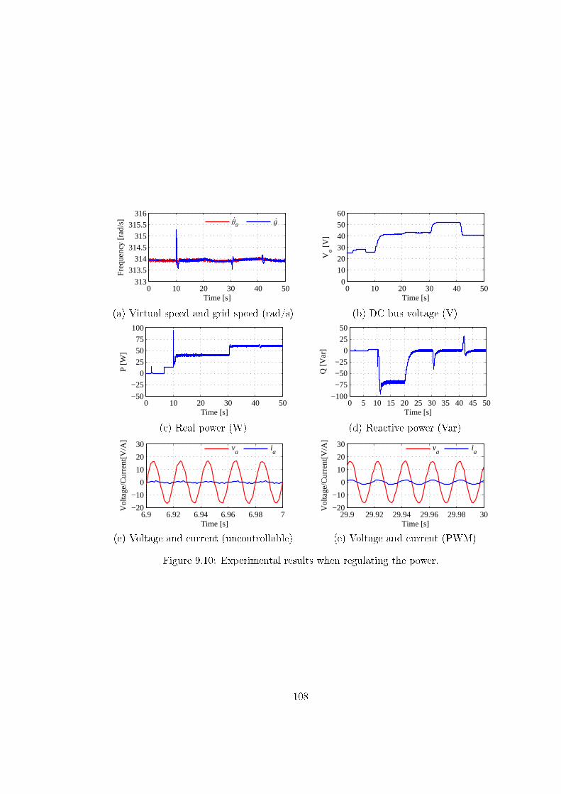
0 10 20 30 40 50313
313.5
314
314.5
315
315.5
316
Time [s]
Freq
uenc
y [r
ad/s
]
θg θ
0 10 20 30 40 500
10
20
30
40
50
60
Vo [
V]
Time [s]
(a) Virtual speed and grid speed (rad/s) (b) DC bus voltage (V)
0 10 20 30 40 50−50
−25
0
25
50
75
100
P [W
]
Time [s]0 5 10 15 20 25 30 35 40 45 50
−100
−75
−50
−25
0
25
50Q
[Var
]
Time [s]
(c) Real power (W) (d) Reactive power (Var)
6.9 6.92 6.94 6.96 6.98 7−20
−10
0
10
20
30
Time [s]
Vol
tage
/Cur
rent
[V/A
]
va
ia
29.9 29.92 29.94 29.96 29.98 30−20
−10
0
10
20
30
Time [s]
Vol
tage
/Cur
rent
[V/A
]
va
ia
(e) Voltage and current (uncontrollable) (e) Voltage and current (PWM)
Figure 9.10: Experimental results when regulating the power.
108
Chapter 10
Synchronverter-based Back-to-back
Converter for Wind Power
During the last decade, more and more attention has been paid to utilising renewable
energy sources to tackle the energy crisis we are facing. Wind power has been regarded
as one of the main alternative renewable power sources to replace/complement fossil
fuels. Wind energy has many advantages such as no pollution, the relatively low capital
cost involved and the short gestation period. Many countries have set strategic plans to
develop technologies for utilising wind power and a lot of researchers have shifted into
this area.
Wind generation systems can be divided into variable-speed generation systems
and xed-speed generation systems. Variable-speed systems are more attractive than
xed-speed systems due to the improved wind energy production and the reduction of
icker problems. Nowadays, the most-used topologies for variable-speed wind turbines
are doubly-fed induction generators with wounded rotors, induction generators with
squirrel cage rotors and synchronous generators with permanent magnets [7]. In these
three cases, one of the most popular grid connection topologies is to adopt back-to-back
voltage source inverters to interface with the grid [10] to provide unity power factor
and low harmonic distortion of current, as shown in Figure 10.1. The synchronous
generator is connected to the grid through a full-scale back-to-back PWM converter
and the conversion stage consists of a rotor-side converter and a grid-side converter. It
has a substantial inuence for power quality, because non-sinusoidal currents delivered
to the grid can introduce an additional non-sinusoidal voltage drop across the line
109
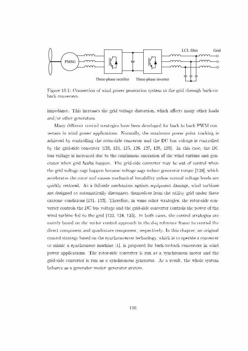
~
Three-phase rectifier Three-phase inverter
LCL filter Grid
PMSG
Figure 10.1: Connection of wind power generation system to the grid through back-to-back converters.
impedance. This increases the grid voltage distortion, which aects many other loads
and/or other generators.
Many dierent control strategies have been developed for back-to-back PWM con-
verters in wind power applications. Normally, the maximum power point tracking is
achieved by controlling the rotor-side converter and the DC bus voltage is controlled
by the grid-side converter [123, 124, 125, 126, 127, 128, 129]. In this case, the DC
bus voltage is increased due to the continuous operation of the wind turbine and gen-
erator when grid faults happen. The grid-side converter may be out of control when
the grid voltage sags happen because voltage sags reduce generator torque [130], which
accelerates the rotor and causes mechanical instability unless normal voltage levels are
quickly restored. As a fail-safe mechanism against equipment damage, wind turbines
are designed to automatically disconnect themselves from the utility grid under these
extreme conditions [131, 132]. Therefore, in some other strategies, the rotor-side con-
verter controls the DC bus voltage and the grid-side converter controls the power of the
wind turbine fed to the grid [133, 134, 135]. In both cases, the control strategies are
mainly based on the vector control approach in the d-q reference frame to control the
direct component and quadrature component, respectively. In this chapter, an original
control strategy based on the synchronverter technology, which is to operate a converter
to mimic a synchronous machine [1], is proposed for back-to-back converters in wind
power applications. The rotor-side converter is run as a synchronous motor and the
grid-side converter is run as a synchronous generator. As a result, the whole system
behaves as a generatormotorgenerator system.
110

10.1 Control of the Rotor-side Converter
As mentioned before, the rotor-side converter is used to maintain a constant DC bus
voltage. Hence, it is run as a PWM rectier. Here, this is done via operating the PWM
rectier to mimic a synchronous motor.
The output voltage and current of the wind-turbine generator are denoted as vr =
[ vra vrb vrc ]T and ir = [ ira irb irc ]T , respectively. The proposed control strat-
egy is shown in Figure 10.2, which includes the model of a synchronous motor as the
core of the control strategy. The model of a synchronous motor is more or less the same
as the model of a generator discussed above, apart from the fact that the direction of
the stator current is dened as opposite. Therefore, Equations (5.1) and (5.3) should
be modied accordingly as
vr = em +Rsir + Lsdirdt,
and
θm =1
Jm(Tme − Tmm −Dmpθm),
where the mechanical torque Tmm is the load to the motor. Here, this is generated by
the PI controller that regulates the DC bus voltage.
The strategy has two channels: one to regulate the real power and the other to
regulate the reactive power. The real power channel shown in Figure 10.2 has three
cascaded control loops. The inner loop is the frequency regulation loop (with the feed-
back gain Dmp); the middle loop is a torque loop (with the feedback coming from the
current ir via the electromagnetic torque Tme) and the outer loop is the DC bus voltage
loop (with the feedback coming from the DC bus voltage Vdc). The rst two loops are
part of the model of a virtual synchronous motor.
When the rotor-side converter is connected to vr, its virtual frequency should track
the frequency of vr. This can be done via feeding the dierence between the frequency
θr obtained from the STA and the rectier frequency θm to the Dmp block, as done
in the synchronverter [1]. In this case, the constant Dmp represents the (imaginary)
mechanical friction coecient of the virtual motor. It is eectively the frequency droop
coecient dened as Dmp = − ∆T∆θm
, which corresponds to a certain amount of change
∆T in the torque leading to a change ∆θm in the frequency.
111

1mK s−
1s STA
PWM Generation 1mJ s PI Dmp
Vref Qm
Qref Mfif Tme Tmm
rθɺ
Reset
θm
vra vr
vr ir
Three-phase rectifier
Eqn.(8.2) Eqn.(8.4) Eqn.(8.6)
PMSG
Vdc
vrb vrc ira
irb irc
mθɺ
em
Vdc ωn
Figure 10.2: Control structure for the rotor-side converter.
The reactive power Qm of the rotor-side converter can be controlled to track the
reference Qref . The tracking error between the reference value Qref and the reactive
power Qm is fed into an integrator with a gain − 1K to regulate the eld excitationMf if
so that the voltage em is changed. In order to obtain the unity power factor, Qref can
be set as 0.
In order for the rotor-side converter, i.e., the virtual synchronous motor, to work
properly, the frequency θm inside the rectier should be the same as, or very close to,
the frequency θr of vr and the terminal voltage should be synchronised with the voltage
vr. Before the rectier is connected to vr, its phase θm should be kept the same as that
of vr in order to minimise the settling time following the connection. The traditional
phase-locked loop (PLL) in the dq frame is not fast enough for this purpose [136]. In
this control strategy, the sinusoid-tracking algorithm (STA) [110] is adopted to provide
the frequency signal and the phase information quickly.
112
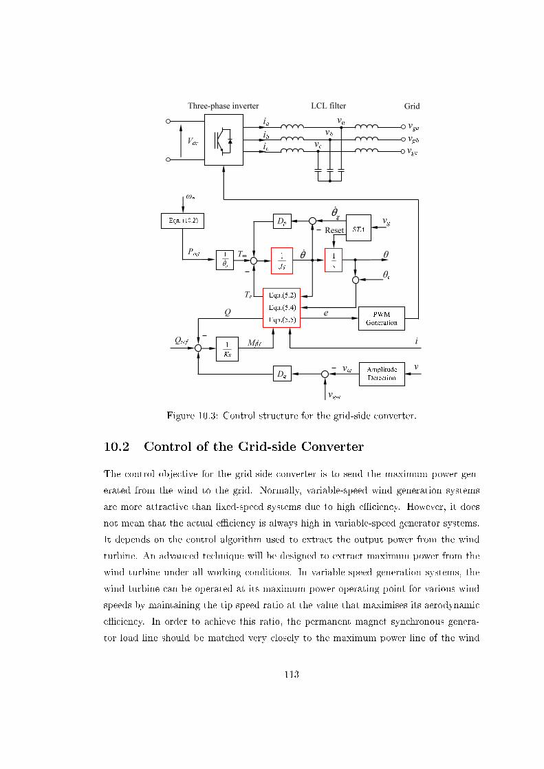
1Ks 1s
STA PWM Generation
1Js Q
Qref Mfif Te Tm
Reset
θ
θc vg
i
Three-phase inverter
Eqn.(5.2) Eqn.(5.4) Eqn.(5.5)
LCL filter
Dp Pref
Dq v
Grid
Amplitude Detection vgm
vm
e
1nθɺ Eqn. (10.2)
va vb
vc ia ib ic vga
vgb vgc
θɺ
Vdc ωn gθɺ
Figure 10.3: Control structure for the grid-side converter.
10.2 Control of the Grid-side Converter
The control objective for the grid-side converter is to send the maximum power gen-
erated from the wind to the grid. Normally, variable-speed wind generation systems
are more attractive than xed-speed systems due to high eciency. However, it does
not mean that the actual eciency is always high in variable-speed generator systems.
It depends on the control algorithm used to extract the output power from the wind
turbine. An advanced technique will be designed to extract maximum power from the
wind turbine under all working conditions. In variable-speed generation systems, the
wind turbine can be operated at its maximum power operating point for various wind
speeds by maintaining the tip speed ratio at the value that maximises its aerodynamic
eciency. In order to achieve this ratio, the permanent magnet synchronous genera-
tor load line should be matched very closely to the maximum power line of the wind
113
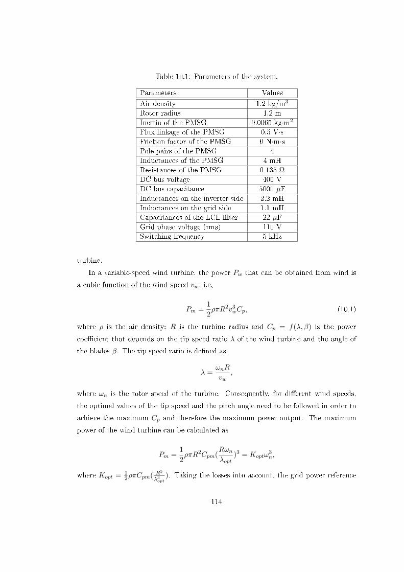
Table 10.1: Parameters of the system.
Parameters ValuesAir density 1.2 kg/m3
Rotor radius 1.2 mInertia of the PMSG 0.0065 kg·m2
Flux linkage of the PMSG 0.5 V·sFriction factor of the PMSG 0 N·m·sPole pairs of the PMSG 4Inductances of the PMSG 4 mHResistances of the PMSG 0.135 Ω
DC bus voltage 400 VDC bus capacitance 5000 µFInductances on the inverter side 2.2 mHInductances on the grid side 1.1 mHCapacitances of the LCL lter 22 µFGrid phase voltage (rms) 110 VSwitching frequency 5 kHz
turbine.
In a variable-speed wind turbine, the power Pw that can be obtained from wind is
a cubic function of the wind speed vw, i.e,
Pm =1
2ρπR2v3
wCp, (10.1)
where ρ is the air density; R is the turbine radius and Cp = f(λ, β) is the power
coecient that depends on the tip speed ratio λ of the wind turbine and the angle of
the blades β. The tip speed ratio is dened as
λ =ωnR
vw,
where ωn is the rotor speed of the turbine. Consequently, for dierent wind speeds,
the optimal values of the tip speed and the pitch angle need to be followed in order to
achieve the maximum Cp and therefore the maximum power output. The maximum
power of the wind turbine can be calculated as
Pm =1
2ρπR2Cpm(
Rωnλopt
)3 = Koptω3n,
where Kopt = 12ρπCpm( R5
λ3opt). Taking the losses into account, the grid power reference
114

Table 10.2: Control parameters for the rotor-side converter.
Parameters Values Parameters ValuesJm 0.0122 Kp 0.8Dmp 6.0793 Ki 2Km 2430.1
Table 10.3: Control parameters for the grid-side converter.
Parameters Values Parameters ValuesJ 0.0122 K 2430.1Dp 6.0793 Dq 386.7615
can be chosen to be slightly smaller than Pm. Here, this is chosen as
Pref = 0.95Koptω3n. (10.2)
This reference can be passed to the synchronverter so that the right amount of power
is fed into the grid. The proposed control strategy for the grid-side converter is shown
in Figure 10.3, where the inductor current, the capacitor voltage and the grid voltage
are denoted as i = [ ia ib ic ]T , v = [ va vb vc ]T and vg = [ vga vgb vgc ]T ,
respectively. This is very similar to the controller for the synchronverter [1], with the
real power reference set as Equation (10.2). Because of the inherent capability of the
synchronverter, this strategy is able to feed the real power to the grid while regulating
the reactive power.
10.3 Simulation Results
Simulations were carried out to verify the control strategy described above in Matlab
7.6/ Simulink/ SimpowerSystems. The solver used in the simulations was ode23t with
a relative tolerance of 10−3 and the sampling time was 2 µs. The parameters of the
system used in the simulations are given in Table 9.1.
The wind turbine extracts power from the wind and then converts it into mechanical
power. The power coecient Cp is calculated by using the following formula [23]:
Cp(λ, β) = 0.22(116
β− 0.4− 5)e
− 12.5β
115
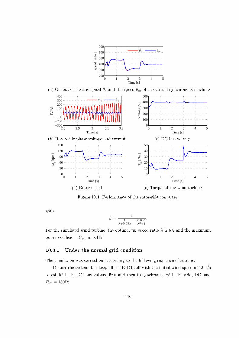
0 1 2 3 4 5200
300
400
500
600
700
Time [s]
spee
d [r
ad/s
]
θr θm
(a) Generator electric speed θr and the speed θm of the virtual synchronous machine
2.8 2.9 3 3.1 3.2−300−200−100
0100200300400
Time [s]
[V/A
]
v
raira
0 1 2 3 4 50
100
200
300
400
500
Vol
tage
[V
]
Time [s]
(b) Rotor-side phase voltage and current (c) DC bus voltage
0 1 2 3 4 50
30
60
90
120
150
ωn [
rpm
]
Time [s]0 1 2 3 4 5
0
10
20
30
40
50
Tm
[N
m]
Time [s]
(d) Rotor speed (e) Torque of the wind turbine
Figure 10.4: Performance of the rotor-side converter.
with
β =1
1λ+0.08λ −
0.035λ3+1
.
For the simulated wind turbine, the optimal tip speed ratio λ is 6.8 and the maximum
power coecient Cpm is 0.419.
10.3.1 Under the normal grid condition
The simulation was carried out according to the following sequence of actions:
1) start the system, but keep all the IGBTs o with the initial wind speed of 12m/s
to establish the DC bus voltage rst and then to synchronise with the grid, DC load
Rdc = 150Ω;
116
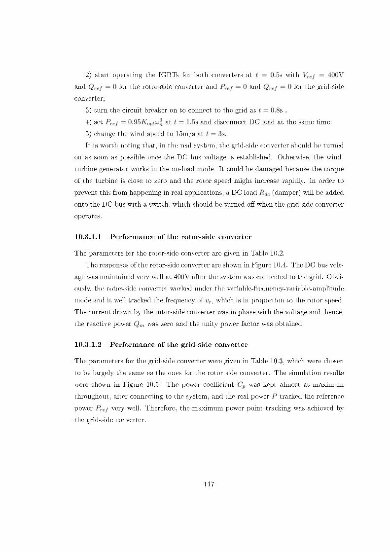
2) start operating the IGBTs for both converters at t = 0.5s with Vref = 400V
and Qref = 0 for the rotor-side converter and Pref = 0 and Qref = 0 for the grid-side
converter;
3) turn the circuit breaker on to connect to the grid at t = 0.8s .
4) set Pref = 0.95Koptω3n at t = 1.5s and disconnect DC load at the same time;
5) change the wind speed to 15m/s at t = 3s.
It is worth noting that, in the real system, the grid-side converter should be turned
on as soon as possible once the DC bus voltage is established. Otherwise, the wind-
turbine generator works in the no-load mode. It could be damaged because the torque
of the turbine is close to zero and the rotor speed might increase rapidly. In order to
prevent this from happening in real applications, a DC load Rdc (damper) will be added
onto the DC bus with a switch, which should be turned o when the grid side converter
operates.
10.3.1.1 Performance of the rotor-side converter
The parameters for the rotor-side converter are given in Table 10.2.
The responses of the rotor-side converter are shown in Figure 10.4. The DC bus volt-
age was maintained very well at 400V after the system was connected to the grid. Obvi-
ously, the rotor-side converter worked under the variable-frequency-variable-amplitude
mode and it well tracked the frequency of vr, which is in proportion to the rotor speed.
The current drawn by the rotor-side converter was in phase with the voltage and, hence,
the reactive power Qm was zero and the unity power factor was obtained.
10.3.1.2 Performance of the grid-side converter
The parameters for the grid-side converter were given in Table 10.3, which were chosen
to be largely the same as the ones for the rotor-side converter. The simulation results
were shown in Figure 10.5. The power coecient Cp was kept almost at maximum
throughout, after connecting to the system, and the real power P tracked the reference
power Pref very well. Therefore, the maximum power point tracking was achieved by
the grid-side converter.
117

0 1 2 3 4 5300
305
310
315
320
325
330
Time [s]
spee
d [r
ad/s
]
θg θ
(a) Grid speed θg and the speed θ of the virtual synchronous machine
2.8 2.9 3 3.1 3.2−200
−100
0
100
200
300
Time [s]
[V/A
]
v
gaia
0 1 2 3 4 50
0.1
0.2
0.3
0.4
0.5
Cp
Time [s]
(b) Grid-side phase voltage and current (c) Power coecient of the wind turbine
0 1 2 3 4 50
1000
2000
3000
4000
5000
Time [s]
P [W
]
P
ref P
0 1 2 3 4 5−1000
−500
0
500
1000
Q [V
ar]
Time [s]
(d) Power reference and real power (e) Reactive power on grid-side converter
Figure 10.5: Performance of the grid-side converter.
10.3.2 Under grid voltage sags
Grid-voltage sags are transient dips in the grid operating voltage, ranging between
10% and 90% of the nominal value and lasting from a few milliseconds to a minute
[132]. Faults resulting from voltage sags can occur on the distribution system or on the
utility system. The new regulations on power grid operation require that wind turbine
systems remain connected with the grid even in the situation of grid-voltage sags to help
the system rapidly recover to the rated output after the fault clearance. Simulations
were carried out to demonstrate the performance of the proposed control strategy in
responding to voltage sags.
In the simulation, the sequence of actions was the same as in the previous case
118

0 1 2 3 4 50
0.1
0.2
0.3
0.4
0.5
Cp
Time [s]0 1 2 3 4 5
0
40
80
120
160
200
Time [s]
[V/A
]
v
gaia
(a) Power coecient of wind turbine (b) RMS of grid-side voltage and current
0 1 2 3 4 50
30
60
90
120
150
ωn [
rpm
]
Time [s]0 1 2 3 4 5
0
10
20
30
40
50
Tm
[N
m]
Time [s]
(c) Rotor speed (d) Torque of the wind turbine
0 1 2 3 4 5−1000
0
1000
2000
3000
4000
5000
Time [s]
P [W
]
P
ref P
0 1 2 3 4 50
100
200
300
400
500V
olta
ge [
V]
Time [s]
(e) Real power of grid-side (f) DC bus voltage
Figure 10.6: System responses during grid voltage sags.
except that the fth action was replaced with the grid voltage drop of 20% at t = 3s.
The system responses are shown in Figure 10.6. The current of the grid side had a
jump when the grid voltage dropped, but it quickly settled down at a value which was
20% higher. There was no noticeable change in the torque and the rotor speed, which
meant that the wind turbine and the PMSG worked properly during the grid voltage
sags. The DC bus voltage was controlled very well by the rotor-side converter and the
maximum power coecient was also maintained.
119

10.4 Conclusions
In this chapter, a synchronverter-based control strategy was proposed for back-to-back
converters applied to a variable speed wind turbine with PMSG. This method is based on
the DC bus voltage controlled by the generator side converter. The grid side converter
controls the grid power according to the MPPT strategy. Moreover, the proposed
control strategy improves the fault ride-through capability and causes the wind turbine
to remain normal when the grid voltage sags. In order to validate the proposed control
strategy, simulation results are provided.
120

Chapter 11
Conclusions and Further Work
11.1 Conclusions
Two of the most popular AC-DC-AC topologies for wind power with PMSG have been
investigated in this thesis.
11.1.1 Uncontrollable rectier + boost converter + inverter
An experimental setup has been designed and built for this AC-DC-AC topology. Based
on this experimental setup, a current control for maximum power point tracking without
a mechanical sensor has been proposed. For constant excitation, the rotating speed of
the generator is proportional to the peak output voltage and the torque of the machine
is proportional to the peak output current. The output current of an uncontrollable
rectier can be controlled by a boost converter according to a current reference, which
is determined by a climbing algorithm, to achieve MPPT.
An inverter is controlled according to the synchronverter technology to implement
the grid-connection. It is able to send a set power to the grid and is also able to
take part in the regulation of the system frequency and voltage. A controller based
on synchronverters for parallel operation of inverters in the stand-alone mode has been
proposed. Based on the droop method, the controller avoids the use of communication
signals among the units. The control strategy consists of a frequency droop loop and a
voltage droop loop which allows for the sharing of the real power and reactive power,
respectively. The concept of capacitive output impedance is adopted to reduce the THD
of the synchronverter's output voltage. Both simulation and experimental results have
been provided.
121
11.1.2 Back-to-back converter
Synchronverter-based control strategies for three-phase rectiers, which can possess
most of the characteristics of conventional synchronous motors, have been proposed.
Therefore, when PWM rectiers are connected with the utility grid, the previous op-
eration methods of the utility grid can still be used regardless of the particular load
characteristics, and the stability of the utility grid can be improved accordingly. In the
proposed schemes, the real power extracted from the source and the output voltage are
the control variables, respectively, hence they can be employed in dierent applications.
Furthermore, improved control schemes without the need of an extra synchronisation
unit have been presented to reduce the computational burden of the controller.
Finally, a control strategy based on the synchronverter technology was proposed for
the back-to-back PWM converter. Both converters are run as synchronverters, which are
mathematically equivalent to the conventional synchronous machines. The rotor-side
converter is responsible for maintaining the DC bus voltage and the grid-side converter
is responsible for the Maximum Power Point Tracking.
11.2 Further Work
Based on the study carried out, various issues can be taken care of in further work, and
are detailed below.
Firstly, synchronverter-based control strategies for three-phase rectiers work in the
simulations. However, the voltage and power used in the experiments in this work
are very low. In order to validate the concept at real voltage and power ratings, the
experiments should be carried out in a more realistic situations.
Secondly, the improved control strategies, which have no need of an extra synchron-
isation unit, have not been applied in back-to-back converters. These control strategies
should work on the grid-side because of the nearly constant frequency of the utility grid.
On the rotor-side, the frequency of the generator output voltage is no longer constant.
Further work should focus on the parameter selection to allow three-phase rectiers to
track the generator frequency properly.
Thirdly, various strategies have been proposed to control PWM rectiers or inverters.
These strategies can achieve the same major goals, such as a high power factor and near-
sinusoidal current waveforms, but they are often based on dierent principles, such as
d-p transformation, VOC, PWM and so on. An overall comparison between them should
122

be given to point out advantages and disadvantages for each other so that we are able to
know which strategy is most appropriate way in dierent situations and requirements.
Fourthly, most of experiments have been implemented in ideal conditions. But there
are large numbers of extreme cases in realistic situations. If we want to apply this way
into practice, many experiments and research should be done to know the fault tolerance
of system in dierent extreme cases.
Moreover, robust control is a branch of control theory that explicitly deals with
uncertainty in its approach to controller design. Robust control methods are designed
to function properly so long as uncertain parameters or disturbances are within some
set. Robust methods aim to achieve robust performance and/or stability in the presence
of bounded modeling errors. Further research about parameters variation should be
investigated. For example, because there is no delay involved in the frequency droop
loop, the time constant can be made much smaller than for a real SG. It is not necessary
to have a large inertia as with a physical SG, where a larger inertia means that more
energy is stored mechanically. Whether a small inertia is good for overall grid stability
is an open question for later research.
Finally, in this work, the prototype of the control strategy for wind power is presen-
ted, however many details could be improved in realistic situations. For example, MPPT
tracking based only on the wind speed is not realistic, since it is dicult to obtain a
realistic value for it. A new experimental setup for the back-to-back converter could be
designed and relevant experiments carried out in realistic environments.
123

References
[1] Q.-C. Zhong and G. Weiss. Synchronverters: Inverters that mimic synchronous
generators. IEEE Trans. Ind. Electron., 58(4):12591267, Apr. 2011.
[2] H.-J. Wagner and J. Mathur. Introduction to wind energy systems: basics, tech-
nology and operation. Springer-Verlag, 2009.
[3] S. Mathew. Wind energy : fundamentals, resource analysis and economics.
Springer-Verlag, 2006.
[4] T. Burton. Wind energy: handbook. John Wiley & Sons, 2001.
[5] S. Heier. Grid integration of wind energy conversion systems. John Wiley & Sons,
2006.
[6] J.F. Manwell, J.G. McGowan, and A.L. Rogers. Wind Energy Explained: Theory,
Design and Application. John Wiley & Sons, 2009.
[7] D.A. Spera. Wind turbine technology: fundamental concepts of wind turbine en-
gineering. ASME Press, 2009.
[8] M. Tazil, V. Kumar, R. C. Bansal, S. Kong, Z. Y. Dong, W. Freitas, and H. D.
Mathur. Three-phase doubly fed induction generators: An overview. IET Proc.
Electric Power Appli., 4(2):7589, 2010.
[9] J. Ekanayake, L. Holdsworth, and N. Jenkins. Control of DFIG wind turbines.
Power Engineer, 17(1):2832, Feb. 2003.
[10] J.A. Baroudi, V. Dinavahi, and A.M. Knight. A review of power converter topolo-
gies for wind generators. In Proc. of IEEE International Conference on Electric
Machines and Drives, pages 458465, May 2005.
124
[11] F.D. Bianchi, H.D. Battista, and R.J. Mantz. Wind turbine control systems:
principles, modelling and gain scheduling design. Springer-Verlag, 2007.
[12] S. Mathew and G.S. Philip. Advances in wind energy and conversion technology.
Springer-Verlag, 2011.
[13] T. Tanaka, T. Toumiya, and T. Suzuki. Output control by hill-climbing method
for a small scale wind power generating system. Renewable Energy, 12(4):387400,
Jul. 1997.
[14] M.G. Simoes, B.K. Bose, and R.J. Spiegel. Fuzzy logic based intelligent control
of a variable speed cage machine wind generation system. In Proc. of Power
Electronics Specialists Conference (PESC), pages 389395, 1995.
[15] K. Tan and S. Islam. Optimum control strategies in energy conversion of pmsg
wind turbine system without mechanical sensors. IEEE Trans. Energy Convers.,
19(2):392399, Jun. 2004.
[16] Quincy Wang and Liuchen Chang. An intelligent maximum power extraction
algorithm for inverter-based variable speed wind turbine systems. IEEE Trans.
Power Del., 19(5):12421249, Sept. 2004.
[17] R. Datta and V.T. Ranganathan. A method of tracking the peak power points
for a variable speed wind energy conversion system. IEEE Power Eng. Rev.,
22(10):5757, Oct. 2002.
[18] E. Koutroulis and K. Kalaitzakis. Design of a maximum power tracking system for
wind-energy-conversion applications. IEEE Trans. Ind. Electron., 53(2):486494,
Apr. 2006.
[19] Ying-Yi Hong, Shiue-Der Lu, and Ching-Sheng Chiou. MPPT for PM wind
generator using gradient approximation. Energy Conversion and Management,
50(1):8289, Aug. 2009.
[20] M.E. Haque, K.M. Muttaqi, and M. Negnevitsky. Control of a standalone variable
speed wind turbine with a permanent magnet synchronous generator. In Proc. of
the 21st Power and Energy Society General Meeting, pages 19, 2008.
125
[21] K. Amei, Y. Takayasu, T. Ohji, and M. Sakui. A maximum power control of
wind generator system using a permanent magnet synchronous generator and a
boost chopper circuit. In Proc. of Power Conversion Conference (PCC), pages
14471452, 2002.
[22] A.B. Kulkarni and M. Ehsani. A novel position sensor elimination technique for
the interior permanent-magnet synchronous motor drive. In Proc. of Industry
Applications Society Annual Meeting, pages 773779, 1989.
[23] Tao Sun, Zhe Chen, and F. Blaabjerg. Voltage recovery of grid-connected wind
turbines after a short-circuit fault. In Proc. of Industrial Electronics Society
(IECON), pages 27232728, 2003.
[24] E. Figueres, G. Garcera, J. Sandia, F. Gonzalez-Espin, and J.C. Rubio. Sensitivity
study of the dynamics of three-phase photovoltaic inverters with an lcl grid lter.
IEEE Trans. Ind. Electron., 56(3):706717, Mar. 2009.
[25] S. Alepuz, S. Busquets-Monge, J. Bordonau, J. Gago, D. Gonzalez, and J. Balcells.
Interfacing renewable energy sources to the utility grid using a three-level inverter.
IEEE Trans. Ind. Electron., 53(5):15041511, Oct. 2006.
[26] J.M. Espi Huerta, J. Castello-Moreno, J.R. Fischer, and R. Garcia-Gil. A syn-
chronous reference frame robust predictive current control for three-phase grid-
connected inverters. IEEE Trans. Ind. Electron., 57(3):954 962, Mar. 2010.
[27] B. Sahan, A.N. Vergara, N. Henze, A. Engler, and P. Zacharias. A single-stage PV
module integrated converter based on a low-power current-source inverter. IEEE
Trans. Ind. Electron., 55(7):26022609, Jul. 2008.
[28] J.M. Espi, J. Castello, R. Garci anda Gil, G. Garcera, and E. Figueres. An
adaptive robust predictive current control for three-phase grid-connected invert-
ers. IEEE Trans. Ind. Electron., 58(8):35373546, Aug. 2011.
[29] R. Kadri, J.-P. Gaubert, and G. Champenois. An improved maximum power
point tracking for photovoltaic grid-connected inverter based on voltage-oriented
control. IEEE Trans. Ind. Electron., 58(1):6675, Jan. 2011.
126

[30] M.P. Kazmierkowski and L. Malesani. Current control techniques for three-phase
voltage-source pwm converters: a survey. IEEE Trans. Ind. Electron., 45(5):691
703, Oct. 1998.
[31] Lidong Zhang, L. Harnefors, and H.-P. Nee. Power-synchronization control of
grid-connected voltage-source converters. IEEE Trans. Power Syst., 25(2):809
820, May 2010.
[32] Theodore Wildi. Electrical Machines, Drives and Power Systems. Prentice-Hall,
6 edition, 2005.
[33] A. Cetin and M. Ermis. VSC-Based D-STATCOM with selective harmonic elim-
ination. IEEE Trans. Ind. Appl., 45(3):10001015, may-jun 2009.
[34] B. Singh, R. Saha, A. Chandra, and K. Al-Haddad. Static synchronous compen-
sators (STATCOM): A review. IET Proc. Power Electron., 2(4):297324, Jul.
2009.
[35] H.-P. Beck and R. Hesse. Virtual synchronous machine. In Proc. of the 9th
International Conference on Electrical Power Quality and Utilisation (EPQU),
pages 16, 2007.
[36] J. Driesen and K. Visscher. Virtual synchronous generators. In Proc. of IEEE
Power and Energy Society General Meeting, pages 13, 2008.
[37] K. Visscher and S.W.H. De Haan. Virtual synchronous machines (VSG's) for
frequency stabilisation in future grids with a signicant share of decentralized
generation. In Proc. of IET-CIRED Seminar on Smart Grids for Distribution,
pages 14, 2008.
[38] M. Torres and L. A. C. Lopes. Frequency control improvement in an autonomous
power system: An application of virtual synchronous machines. In Proc. of the
8th IEEE International Conference on Power Electronics and ECCE Asia (ICPE
& ECCE), pages 21882195, 2011.
[39] Y. Chen, R. Hesse, D. Turschner, and H.-P. Beck. Improving the grid power
quality using virtual synchronous machines. In Proc. of International Conference
on Power Engineering, Energy and Electrical Drives (POWERENG), pages 16,
2011.
127

[40] Q.-C. Zhong and G. Weiss. Static synchronous generators for distributed genera-
tion and renewable energy. In Proc. of IEEE PES Power Systems Conference &
Exhibition (PSCE), 2009.
[41] R.H. Lasseter. Microgrids. In Proc. of IEEE Power Engineering Society Winter
Meeting, pages 305308, 2002.
[42] Tomas Hornik. Power quality in microgrids. PhD thesis, University of Liverpool,
Liverpool, UK, 2010.
[43] F. Katiraei, R. Iravani, N. Hatziargyriou, and A. Dimeas. Microgrids management.
IEEE Power Energy Mag., 6(3):5465, May/Jun. 2008.
[44] C. Xiarnay, H. Asano, S. Papathanassiou, and G. Strbac. Policymaking for mi-
crogrids. IEEE Power Energy Mag., 6(3):6677, May/Jun. 2008.
[45] H. Nikkhajoei and R.H. Lasseter. Distributed generation interface to the CERTS
microgrid. IEEE Trans. Power Del., 24(3):15981608, Jul. 2009.
[46] Shiguo Luo, Zhihong Ye, Ray-Lee Lin, and F.C. Lee. A classication and eval-
uation of paralleling methods for power supply modules. In Power Electronics
Specialists Conference, 1999. PESC 99. 30th Annual IEEE, pages 901 908 vol.2,
1999.
[47] C.S. Lee, S. Kim, C.B. Kim, S.C. Hong, J.S. Yoo, S.W. Kim, C.H. Kim, S.H.
Woo, and S.Y. Sun. Parallel ups with a instantaneous current sharing control. In
Industrial Electronics Society, 1998. IECON '98. Proceedings of the 24th Annual
Conference of the IEEE, pages 568 573 vol.1, Aug 1998.
[48] Jiann-Fuh Chen and Ching-Lung Chu. Combination voltage-controlled and
current-controlled pwm inverters for ups parallel operation. Power Electronics,
IEEE Transactions on, 10:547 558, Sept 1995.
[49] T. Kawabata and S. Higashino. Parallel operation of voltage source inverters.
Industry Applications, IEEE Transactions on, 24(2):281 287, mar/apr 1988.
[50] A.P. Martins, A.S. Carvalho, and A.S. Araujo. Design and implementation of
a current controller for the parallel operation of standard upss. In Industrial
Electronics, Control, and Instrumentation, 1995., Proceedings of the 1995 IEEE
128
IECON 21st International Conference on, volume 1, pages 584 589 vol.1, Nov
1995.
[51] Tsai-Fu Wu, Yu-Kai Chen, and Yong-Heh Huang. 3c strategy for inverters in
parallel operation achieving an equal current distribution. Industrial Electronics,
IEEE Transactions on, 47(2):273 281, Apr 2000.
[52] J.M. Guerrero, L. Garcia de Vicuna, J. Matas, and J. Castilla, M. andMiret.
Output impedance design of parallel-connected UPS inverters with wireless load-
sharing control. IEEE Trans. Ind. Electron., 52(4):11261135, May. 2005.
[53] J.M. Guerrero, J. Matas, Luis Garcia de Vicuna, M. Castilla, and J. Miret. De-
centralized control for parallel operation of distributed generation inverters using
resistive output impedance. IEEE Trans. Ind. Electron., 54(2):9941004, Nov.
2007.
[54] E. Barklund, N. Pogaku, M. Prodanovic, C. Hernandez-Aramburo, and T.C.
Green. Energy management in autonomous microgrid using stability-constrained
droop control of inverters. IEEE Trans. Power Electron., 23(5):23462352, Sept.
2008.
[55] Y. Mohamed and E.F. El-Saadany. Adaptive decentralized droop controller to
preserve power sharing stability of paralleled inverters in distributed generation
microgrids. IEEE Trans. Power Electron., 23(6):28062816, Nov. 2008.
[56] J. M. Guerrero, J. C. Vasquez, J. matas, L. Garcia de Vicuna, and M. Castilla. Hi-
erarchical control of droop-controlled AC and DC microgrids- a general approach
towards standardization. IEEE Trans. Ind. Electron., 58(1):158172, Jan. 2011.
[57] A. Tuladhar, H. Jin, T. Unger, and K. Mauch. Parallel operation of single phase
inverter modules with no control interconnections. In Proc. of the 12th IEEE
Applied Power Electronics Conference and Exposition, pages 94100, 1997.
[58] R. Majumder, B. Chaudhuri, A. Ghosh, G. Ledwich, and F. Zare. Improvement
of stability and load sharing in an autonomous microgrid using supplementary
droop control loop. IEEE Trans. Power Syst., 25(2):796808, May 2010.
129

[59] K. De Brabandere, B. Bolsens, J. Van den Keybus, A. Woyte, J. Driesen, and
R. Belmans. A voltage and frequency droop control method for parallel inverters.
IEEE Trans. Power Electron., 22(4):11071115, Jul. 2007.
[60] G. Diaz, C. Gonzalez-Moran, J. Gomez-Aleixandre, and A. Diez. Scheduling
of droop coecients for frequency and voltage regulation in isolated microgrids.
IEEE Trans. Power Syst., 25(1):489496, Feb. 2010.
[61] M.C. Chandorkar, D.M. Divan, and R. Adapa. Control of parallel connected
inverters in standalone AC supply systems. IEEE Trans. Ind. Appl., 29(1):136
143, Jan./Feb. 1993.
[62] U. Borup, F. Blaabjerg, and P.N. Enjeti. Sharing of nonlinear load in parallel-
connected three-phase converters. IEEE Trans. Ind. Appl., 37(6):18171823,
Nov./Dec. 2001.
[63] E.A.A. Coelho, P.C. Cortizo, and P.F.D. Garcia. Small-signal stability for parallel-
connected inverters in stand-alone AC supply systems. IEEE Trans. Ind. Appl.,
38(2):533542, Oct. 2002.
[64] J.M. Guerrero, L.G. de Vicuna, J. Miret, J. Matas, and J. Cruz. Output
impedance performance for parallel operation of UPS inverters using wireless and
average current-sharing controllers. In Proc. of the 35th IEEE Power Electronics
Specialists Conference, pages 24822488, 2004.
[65] J.M. Guerrero, N. Berbel, L.G. de Vicuna, J. Matas, J. Miret, and M. Castilla.
Droop control method for the parallel operation of online uninterruptible power
systems using resistive output impedance. In Proc. of the 21st IEEE Applied
Power Electronics Conference and Exposition, pages 17161722, 2006.
[66] A. Tuladhar, Hua Jin, T. Unger, and K. Mauch. Control of parallel inverters in
distributed AC power systems with consideration of line impedance eect. IEEE
Trans. Ind. Appl., 36(1):131138, Jan./Feb. 2000.
[67] Chien-Liang Chen, Yubin Wang, Jih-Sheng Lai, Yuang-Shung Lee, and D. Martin.
Design of parallel inverters for smooth mode transfer microgrid applications. IEEE
Trans. Power Electron., 25(1):615, Feb. 2010.
130
[68] T. Ackerman. Wind Power in Power Systems. Chichester: John Wiley & Sons,
Ltd., 2005.
[69] F. Blaabjerg, Z. Chen, and S.B. Kjaer. Power electronics as ecient interface in
dispersed power generation systems. IEEE Trans. Power Electron., 19(5):1184
1194, Sept. 2004.
[70] F. Blaabjerg, F. Iov, R. Teodorescu, and Z. Chen. Power electronics in renewable
energy systems. In Proc. of the 12th International Power Electronics and Motion
Control Conference (EPE-PEMC), pages 117, 2006.
[71] G. Weiss, Q.-C. Zhong, T. Green, and J. Liang. H∞ repetitive control of DC-
AC converters in micro-grids. IEEE Trans. Power Electron., 19(1):219230, Jan.
2004.
[72] J.M. Guerrero, J.C. Vasquez, J. Matas, M. Castilla, and L.G. de Vicuna. Con-
trol strategy for exible microgrid based on parallel line-interactive UPS systems.
IEEE Trans. Ind. Electron., 56(3):726736, Mar. 2009.
[73] S. V. Iyer, M. N. Belur, and M. C. Chandorkar. A generalized computational
method to determine stability of a multi-inverter microgrid. IEEE Trans. Power
Electron., 25(9):24202432, Sept. 2010.
[74] T. Hornik and Q.-C. Zhong. A current control strategy for voltage-source inverters
in microgrids based on H∞ and repetitive control. IEEE Trans. Power Electron.,
26(3):943952, Mar. 2011.
[75] N. Yousefpoor, S. Fathi, N. Farokhnia, and H. Askarian Abyaneh. THD mini-
mization applied directly on the line to line voltage of multi-level inverters. IEEE
Trans. Ind. Electron., 59(1):373380, Jan. 2012.
[76] A. V. Timbus, R. Teodorescu, F. Blaabjerg, M. Liserre, and P. Rodriguez. Linear
and nonlinear control of distributed power generation systems. In Proc. of IEEE
Industry Applications Conference, pages 10151023, 2006.
[77] F. Blaabjerg, R. Teodorescu, M. Liserre, and A.V. Timbus. Overview of control
and grid synchronization for distributed power generation systems. IEEE Trans.
Ind. Electron., 53(5):13981409, Oct. 2006.
131

[78] Y.-Y. Tzou, S.-L. Jung, and H.-C. Yeh. Adaptive repetitive control of PWM
inverters for very low THD AC-voltage regulation with unknown loads. IEEE
Trans. Power Electron., 14(5):973981, Sept. 1999.
[79] T. Hornik and Q.-C. Zhong. Voltage control of grid-connected inverters based
on h∞ and repetitive control. In Proc. of the 8th World Congress on Intelligent
Control and Automation (WCICA), pages 270275, 2010.
[80] B.A. Francis and W.M. Wonham. The internal model principle for linear multi-
variable regulators. Applied Mathematics and Optimization, 2(2):170194, 1975.
[81] A. Garcia-Cerrada, O. Pinzon-Ardila, V. Feliu-Batlle, P. Roncero-Sanchez, and
P. Garcia-Gonzalez. Application of a repetitive controller for a three-phase active
power lter. IEEE Trans. Power Electron., 22(1):237246, Jan. 2007.
[82] R. Costa-Castello, R. Grino, R. Cardoner, and E. Fossas. High performance con-
trol of a single-phase shunt active lter. In Proc. of IEEE International Symposium
on Industrial Electronics (ISIE), pages 33503355, 2007.
[83] T. Hornik and Q.-C. Zhong. H∞ repetitive voltage control of grid-connected in-
verters with frequency adaptive mechanism. IET Proc. Power Electron., 3(6):925
935, Nov. 2010.
[84] F. Khatounian, E. Monmasson, F. Berthereau, E. Delaleau, and J.P. Louis. Con-
trol of a doubly fed induction generator for aircraft application. In Proc. of the
29th Annual Conference of the IEEE Industrial Electronics Society, pages 2711
2716, 2003.
[85] F. Khatounian, E. Monmasson, F. Berthereau, and J.P. Louis. Design of an
output LC lter for a doubly fed induction generator supplying non-linear loads
for aircraft applications. In Proc. of IEEE International Symposium on Industrial
Electronics (ISIE), pages 10931098, 2004.
[86] J. Mazumdar, I. Batarseh, N. Kutkut, and O. Demirci. High frequency low cost
DC-AC inverter design with fuel cell source for home applications. In Proc. of
the 37th IAS Annual Meeting and World Conference on Industrial applications of
Electrical Energy, pages 789794, 2002.
132
[87] H.W. Klesser, S.W.H. de Haan, and J.B. Woudstra. Analysis of a controllable
LC-lter for compensation of specic harmonics. In Proc. of Power Electronic
Drives and Energy Systems for Industrial Growth, pages 588591 Vol. 2, 1998.
[88] Timothy C.Y. Wang, Zhihong Ye, Gautam Sinha, and Xiaoming Yuan. Output
lter design for a grid-interconnected three-phase inverter. In Proc. of the 34th
Annual IEEE Power Electronics Specialists Conference, volume 2, pages 779784,
2003.
[89] Q.-C. Zhong and Y. Zeng. Can the output impedance of an inverter be designed
capacitive? In Proc. of the 37th Annual IEEE Conference of Industrial Electronics
(IECON), 2011.
[90] Q.-C. Zhong and Y. Zeng. Inverters with optimal capacitive output impedances
to minimise the output voltage THD. under review.
[91] Q.-C. Zhong, F. Blaabjerg, J.M. Guerrero, and T. Hornik. Reduction of voltage
harmonics for parallel-operated inverters. In Proc. of IEEE Energy Conversion
Congress and Exposition (ECCE), pages 473478, 2011.
[92] Guoqiao Shen, Xuancai Zhu, Jun Zhang, and Dehong Xu. A new feedback method
for PR current control of LCL-lter-based grid-connected inverter. IEEE Trans.
Ind. Electron., 57(6):20332041, Jun. 2010.
[93] T. Ericsen, N. Hingorani, and Y. Khersonsky. Power electronics and future marine
electrical systems. IEEE Trans. Ind. Appl., 42(1):155 163, Feb. 2006.
[94] J.R. Rodriguez, J.W. Dixon, J.R. Espinoza, J. Pontt, and P. Lezana. PWM
regenerative rectiers: State of the art. IEEE Trans. Ind. Electron., 52(1):522,
Feb. 2005.
[95] M. Cichowlas, M. Malinowski, M.P. Kazmierkowski, D.L. Sobczuk, P. Rodriguez,
and J. Pou. Active ltering function of three-phase PWM boost rectier under
dierent line voltage conditions. IEEE Trans. Ind. Electron., 52(2):410419, Apr.
2005.
[96] J.W. Dixon and Boon-Teck Ooi. Indirect current control of a unity power factor
sinusoidal current boost type three-phase rectier. IEEE Trans. Ind. Electron.,
35(4):508515, Nov. 1988.
133
[97] S. Hansen, M. Malinowski, F. Blaabjerg, and M.P. Kazmierkowski. Sensorless
control strategies for PWM rectier. In Proc. of Applied Power Electronics Con-
ference and Exposition (APEC), pages 832838, 2000.
[98] K. Zhou and D. Wang. Digital repetitive controlled three-phase PWM rectier.
IEEE Trans. Power Electron., 18(1):309316, Jan. 2003.
[99] J.L. Duarte, A. Van Zwam, C. Wijnands, and A. Vandenput. Reference frames t
for controlling PWM rectiers. IEEE Trans. Ind. Electron., 46(3):628630, Jun.
1999.
[100] M.P. Kazmierkowski and L. Malesani. Current control techniques for three-phase
voltage-source PWM converters: Asurvey. IEEE Trans. Ind. Electron., 45(5):691
703, Oct. 1998.
[101] Dong-Choon Lee and Dae-Sik Lim. AC voltage and current sensorless control of
three-phase PWM rectiers. IEEE Power Electron. Lett., 17(6):883 890, Nov.
2002.
[102] C. Cecati, A. Dell'Aquila, A. Lecci, and M. Liserre. Implementation issues of
a fuzzy-logic-based three-phase active rectier employing only voltage sensors.
IEEE Trans. Ind. Electron., 52(2):378 385, Apr. 2005.
[103] Z. Zhou, P.J. Unsworth, P.M. Holland, and P. Igic. Design and analysis of a feed-
forward control scheme for a three-phase voltage source pulse width modulation
rectier using sensorless load current signal. IET Proc. Power Electron., 2(4):421
430, Jul. 2009.
[104] T. Noguchi, H. Tomiki, S. Kondo, and I. Takahashi. Direct power control of
PWM converter without power-source voltage sensors. IEEE Trans. Ind. Appl.,
34(3):473479, May/Jun. 1998.
[105] M. Malinowski, M.P. Kazmierkowski, S. Hansen, F. Blaabjerg, and G.D. Mar-
ques. Virtual-ux-based direct power control of three-phase PWM rectiers. IEEE
Trans. Ind. Appl., 37(4):10191027, Jul./Aug. 2001.
[106] G. Escobar, A.M. Stankovic, J.M. Carrasco, E. Galvan, and R. Ortega. Analysis
and design of direct power control (DPC) for a three-phase synchronous rectier
134
via output regulation subspaces. IEEE Trans. Power Del., 18(3):823830, May
2003.
[107] M. Malinowski, M. Jasinski, and M.P. Kazmierkowski. Simple direct power control
of three-phase PWM rectier using space-vector modulation (DPC-SVM). IEEE
Trans. Ind. Electron., 51(2):447454, Apr. 2004.
[108] B.S. Chen and G. Joos. Direct power control of active lters with averaged switch-
ing frequency regulation. IEEE Trans. Power Del., 23(6):27292737, Nov. 2008.
[109] Shan Dong-liang, Song Shu-zhong, Ma Jian-wei, and Wang Xian-bo. Direct power
control of PWM rectiers based on virtual ux. In Proc. of the International Con-
ference on Computer Application and System Modeling (ICCASM), pages 613
616, 2010.
[110] A. K. Ziarani and A. Konrad. A method of extraction of nonstationary sinusoids.
Signal Processing, 84(8):13231346, Apr. 2004.
[111] Z. Ma, Q.-C. Zhong, and J. Yan. Synchronverter-based control strategies for
three-phase PWM rectiers. In Proc. of the 7th IEEE Conference on Industrial
Electronics and Applications (ICIEA), Singapore, Jul. 2012.
[112] S.-K. Chung. Phase-locked loop for grid-connected three-phase power conversion
systems. IEE Proc. Electric Power Appli., 147(3):213219, May 2000.
[113] D. Jovcic. Phase locked loop system for FACTS. IEEE Trans. Power Syst.,
18(3):11161124, Aug. 2003.
[114] R.M. Santos Filho, P.F. Seixas, P.C. Cortizo, L.A.B. Torres, and A.F. Souza.
Comparison of three single-phase PLL algorithms for UPS applications. IEEE
Trans. Ind. Electron., 55(8):29232932, Aug. 2008.
[115] C.H. da Silva, R.R. Pereira, L.E.B. da Silva, G. Lambert-Torres, B.K. Bose, and
S.U. Ahn. A digital PLL scheme for three-phase system using modied syn-
chronous reference frame. IEEE Trans. Ind. Electron., 57(11):38143821, Nov.
2010.
135
[116] M. Karimi Ghartemani, A. khajehoddin, P. Jain, and A. Bakhshai. Problems of
startup and phase jumps in PLL systems. IEEE Trans. Power Electron., PP(99):1,
Sept. 2011.
[117] Y.F. Wang and Y.W. Li. Grid synchronization PLL based on cascaded delayed
signal cancellation. IEEE Trans. Power Electron., 26(7):19871997, Jul. 2011.
[118] Dong Dong, D. Boroyevich, P. Mattavelli, and I. Cvetkovic. A high-performance
single-phase phase-locked-loop with fast line-voltage amplitude tracking. In Proc.
of the 26th Annual IEEE Applied Power Electronics Conference and Exposition
(APEC), pages 16221628, 2011.
[119] G. Escobar, M.F. Martinez-Montejano, A.A. Valdez, P.R. Martinez, and
M. Hernandez-Gomez. Fixed-reference-frame phase-locked loop for grid synchro-
nization under unbalanced operation. IEEE Trans. Ind. Electron., 58(5):1943
1951, May 2011.
[120] Xiaoqiang Guo, Weiyang Wu, and Zhe Chen. Multiple-complex coecient-
lter-based phase-locked loop and synchronization technique for three-phase grid-
interfaced converters in distributed utility networks. IEEE Trans. Ind. Electron.,
58(4):11941204, Apr. 2011.
[121] L. Harnefors, M. Bongiorno, and S. Lundberg. Input-admittance calculation and
shaping for controlled voltage-source converters. IEEE Trans. Ind. Electron.,
54(6):33233334, Dec. 2007.
[122] D. Jovcic, L.A. Lamont, and L. Xu. VSC transmission model for analytical studies.
In Proc. of IEEE Power Engineering Society General Meeting, volume 3, pages
17371742, Jul. 2003.
[123] R. Pena, J.C. Clare, and G.M. Asher. Doubly fed induction generator using
back-to-back PWM converters and its application to variable-speed wind-energy
generation. IEE Proc. Electric Power Appli., 143(3):231241, May 1996.
[124] R. Pena, J.C. Clare, and G.M. Asher. A doubly fed induction generator using
back-to-back PWM converters supplying an isolated load from a variable speed
wind turbine. IEE Proc. Electric Power Appli., 143(5):380387, Sept. 1996.
136

[125] R. Cardenas and R. Pena. Sensorless vector control of induction machines
for variable-speed wind energy applications. IEEE Trans. Energy Convers.,
19(1):196205, Mar. 2004.
[126] R. Teodorescu and F. Blaabjerg. Flexible control of small wind turbines with grid
failure detection operating in stand-alone and grid-connected mode. IEEE Trans.
Power Electron., 19(5):13231332, Sept. 2004.
[127] R.C. Portillo, M.M. Prats, J.I. Leon, J.A. Sanchez, J.M. Carrasco, E. Galvan, and
L.G. Franquelo. Modeling strategy for back-to-back three-level converters applied
to high-power wind turbines. IEEE Trans. Ind. Electron., 53(5):14831491, Oct.
2006.
[128] E.J. Bueno, S. Cobreces, F.J. Rodriguez, A. Hernandez, and F. Espinosa. Design
of a back-to-back NPC converter interface for wind turbines with squirrel-cage
induction generator. IEEE Trans. Energy Convers., 23(3):932945, Sept. 2008.
[129] M. Singh, V. Khadkikar, and A. Chandra. Grid synchronisation with harmonics
and reactive power compensation capability of a permanent magnet synchronous
generator-based variable speed wind energy conversion system. IET Proc. Power
Electron., 4(1):122130, Jan. 2011.
[130] O. Gomis-Bellmunt, A. Junyent-Ferre, A. Sumper, and J. Bergas-Jan. Ride-
through control of a doubly fed induction generator under unbalanced voltage
sags. IEEE Trans. Energy Convers., 23(4):10361045, Dec. 2008.
[131] M.F. McGranaghan, D.R. Mueller, and M.J. Samotyj. Voltage sags in industrial
systems. IEEE Trans. Ind. Appl., 29(2):397403, Mar./Apr. 1993.
[132] Math H. Bollen. Understanding Power Quality Problems: Voltage Sags and In-
terruptions. Wiley-IEEE Press, 2000.
[133] Xibo Yuan, Fei Wang, D. Boroyevich, Yongdong Li, and R. Burgos. DC-link
voltage control of a full power converter for wind generator operating in weak-
grid systems. IEEE Trans. Power Del., 24(9):21782192, Sept. 2009.
[134] A.D. Hansen and G. Michalke. Multi-pole permanent magnet synchronous gen-
erator wind turbines' grid support capability in uninterrupted operation during
grid faults. IET Proc. Renewable Power Generation, 3(3):333348, Sept. 2009.
137

[135] Ki-Hong Kim, Yoon-Cheul Jeung, Dong-Choon Lee, and Heung-Geun Kim. Ro-
bust control of PMSG wind turbine systems with back-to-back PWM convert-
ers. In Proc. of the 2nd Power Electronics for Distributed Generation Systems
(PEDG), pages 433437, 2010.
[136] A. K. Ziarani, A. Konrad, and A. N. Sinclair. A novel time-domain method of
analysis of pulsed sine wave signals. IEEE Trans. Instrum. Meas., 52(3):809814,
Jun. 2003.
138

Appendix A
PCB Layout
139
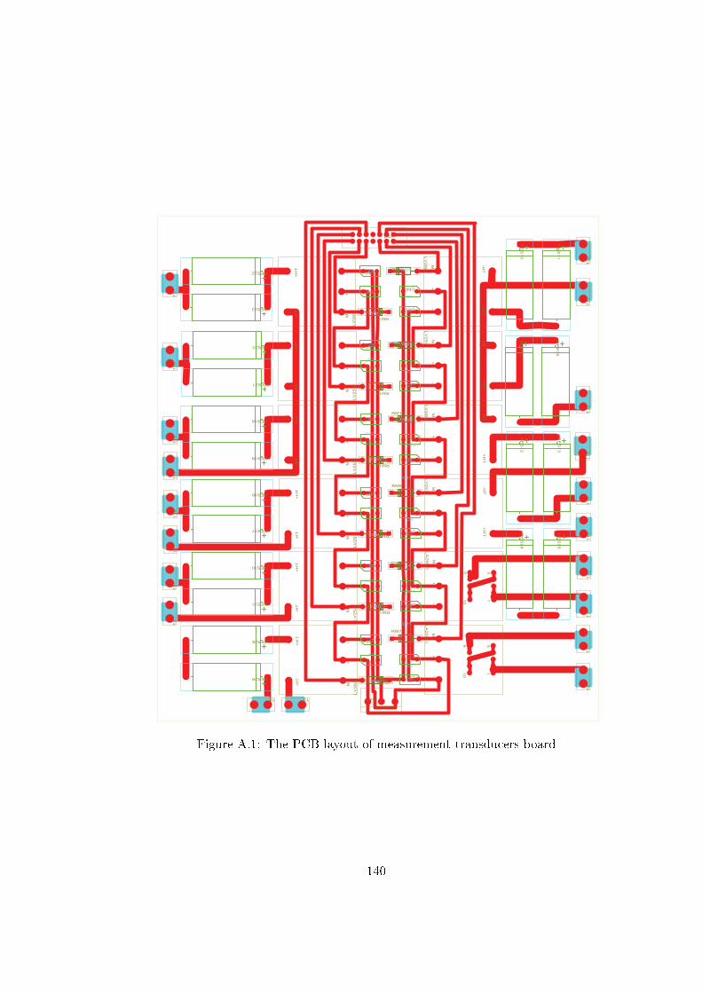
10
6
1
M+
_
5
LA25NS
C66
10
6
1
M+
_
5
LA25NU
C49
C50
C48
C58
C57
C47
M_
+
-HT
+HT
LV25T
M_
+
-HT
+HT
LV25U
M_
+
-HT
+HT
LV25V
C40
C39
C37
C65
M_
+
-HT
+HT
LV26B
RM17
C38
RM7
R16
RM9
RM10
RM11
J16
C60
C59
M_
+
-HT
+HT
LV26A
M_
+
-HT
+HT
LV25Z
C62
C61
M_
+
-HT
+HT
LV25X
M_
+
-HT
+HT
LV25W
C54
C53
C52
C51
C56
C55
M_
+
-HT
+HT
LV25Y
C63
C64
M_
+
-HT
+HT
LV26C
RM15
RM14
RM13
RM12
RM18
RM16
T15
T14
RES28
RES29
RES31
RES17
RES19
RES18
RES20
RES21
RES22
RES16
RES30
T13
T12
CN1
T9
T10
RES10
RES15
T20
RES14
RES12
RES13
RES25
RES11
RES24
T21
T8
T7
T4 T5
T3
T2
T1
T18
T17
T16
T6
T19
RES23
C7
C8
C10
C9
C8
C7
RM2
RM1
C7
C8
C10
C9
RM2
C7
RM1
C8
RM1
C8
C7
RM1
RM1
C7
RM2
R4
C7
C8
C7
C8
C9
C10
RM1
C9
C10
RM1
C8
Figure A.1: The PCB layout of measurement transducers board
140

C83
C79
C80
C82
LM358BP
LM358BQ
R140
R151
R152
R156
R177
R158
R155
R162
R160
R161
R157
C75
C81
R153
C85
C86
C88
LM358BR
LM358BL
R163
R165
R166
R169
R170
R178
R168
R174
C90
R124
R171
C89
C95
C91
C92
C94
LM358BT
LM358BU
R164
R175
R176
R180
R181
R182
R179
R186
R184
R185
C96
C77
C73
C74
C76
LM358BN
LM358BO
R139
R141
R145
R146
R147
R154
R150
R143
C93
C65
C61
C62
C64
LM358BJ
LM358BK
R115
R117
R118
R121
R122
R123
R120
R130
R125
R126
C71
R116
R129
C70
LM358BS
LM358BM
R127
R128
R132
R133
R134
R131
R138
R136
C69
C68
R137
C101
C97
C98
C100
LM358BV
LM358BW
R187
R188
R189
R192
R193
R194
R191
R238
R236
R237
C107
C103
C104
C106
LM358BX
LM358BY
R239
R240
R241
R244
R245
R246
R243
R250
R248
R249
P9
P13
C141
R173
CN1
L11226
T13
RV30
RV31
RV32
RV33
RV34
RV35
RV36
RV37
T14
T15
C164
C177
C176
T16
C165
C166
C167
J1
P18
RV46
RV49
C134 C136 C138 C140 C142 C144 C146 C148
C150C151C152C153C154C155C156C157
LM358CO LM358CP LM358CQ LM358CR LM358CS LM358CT LM358CU LM358CV
R219
R220
R221
R222
R223
R224
R225
R226
R227
R228
R229
R230
R231
R232
R233
R234
CN2
CN4
C161
RV42
RV43
RV44
L11224
L11225
J13
RV38
RV39
RV40
L11222
T12
T17
R149
P10
P11
C179
C178
T2
L17016
L17018
L17019
R167
R183
C67
C72
C63
C66
C84
R159
C87
R172
R135
R119
P16
C143
C170
C171
C172
C173
C135
C137
C139
C145
C147
C149
LM358CW
LM358CX
LM358CY
LM358CZ
LM358DA
LM358DB
LM358DC
LM358DD
R251
R252
R253
R254
R255
R256
R257
R258
R259
R260
R261
R262
R263
R264
R265
R266
C174
C175
LM358DE
LM358DF
R268
R269
R270
R271
C169
C168
C159
C158
C181
C180
T8
T10
T11
P15
T18
C162
L17017
C163
C160
L11223
RV45
RV41
J11
C99
R190
C102
R235
C105
R242
C108
R247
C78
R148
P12
P14
Figure A.2: The PCB layout of control board141

Appendix B
Schematics
142

Figure B.1: Schematics
143

Appendix C
Matlab Code
DigitalInputGUI.m
function varargout = DigitalInputGUI(varargin)
gui_Singleton = 1;
gui_State = struct('gui_Name', mlename, ...
'gui_Singleton', gui_Singleton, ...
'gui_OpeningFcn', @DigitalInputGUI_OpeningFcn, ...
'gui_OutputFcn', @DigitalInputGUI_OutputFcn, ...
'gui_LayoutFcn', [] , ...
'gui_Callback', []);
if nargin && ischar(varargin1)
gui_State.gui_Callback = str2func(varargin1);
end
if nargout
[varargout1:nargout] = gui_mainfcn(gui_State, varargin:);
else
gui_mainfcn(gui_State, varargin:);
end
function DigitalInputGUI_OpeningFcn(hObject, eventdata, handles, varargin)
handles.output = hObject;
guidata(hObject, handles);
global cc;
[cc, err] = PrepareTargetandLoad (handles);
if err == 1
144

return
end
congure(cc.rtdx,1024,8);
open(cc.rtdx,'DigIn0','r');
open(cc.rtdx,'DigIn1','r');
open(cc.rtdx,'DigIn2','r');
open(cc.rtdx,'DigIn3','r');
open(cc.rtdx,'DigIn4','r');
open(cc.rtdx,'DigIn5','r');
open(cc.rtdx,'DigIn6','r');
open(cc.rtdx,'DigIn7','r');
enable(cc.rtdx,'DigIn0');
enable(cc.rtdx,'DigIn1');
enable(cc.rtdx,'DigIn2');
enable(cc.rtdx,'DigIn3');
enable(cc.rtdx,'DigIn4');
enable(cc.rtdx,'DigIn5');
enable(cc.rtdx,'DigIn6');
enable(cc.rtdx,'DigIn7');
enable(cc.rtdx);
cc.rtdx
run(cc);
r = cc.rtdx;
t0 = r.readmsg('DigIn0', 'double');
set(handles.input0, 'string', num2str(t0));
t1 = r.readmsg('DigIn1', 'double');
set(handles.input1, 'string', num2str(t1));
t2 = r.readmsg('DigIn2', 'double');
set(handles.input2, 'string', num2str(t2));
t3 = r.readmsg('DigIn3', 'double');
set(handles.input3, 'string', num2str(t3));
t4 = r.readmsg('DigIn4', 'double');
set(handles.input4, 'string', num2str(t4));
t5 = r.readmsg('DigIn5', 'double');
145

set(handles.input5, 'string', num2str(t5));
t6 = r.readmsg('DigIn6', 'double');
set(handles.input6, 'string', num2str(t6));
t7 = r.readmsg('DigIn7', 'double');
set(handles.input7, 'string', num2str(t7));
set(handles.gure1,'visible','on');
while(isenabled(cc.rtdx))
pause(0.5);
numMsgs0 = r.msgcount('DigIn0');
if (numMsgs0 > 0),
if (numMsgs0 > 1),
r.ush('DigIn0',numMsgs0-1);
end
t0 = r.readmsg('DigIn0', 'double');
end
set(handles.input0, 'string', num2str(t0));
numMsgs1 = r.msgcount('DigIn1');
if (numMsgs1 > 0),
if (numMsgs1 > 1),
r.ush('DigIn1',numMsgs1-1);
end
t1 = r.readmsg('DigIn1', 'double');
end
set(handles.input1, 'string', num2str(t1));
numMsgs2 = r.msgcount('DigIn2');
if (numMsgs2 > 0),
if (numMsgs2 > 1),
r.ush('DigIn2',numMsgs2-1);
end
t2 = r.readmsg('DigIn2', 'double');
end
set(handles.input2, 'string', num2str(t2));
numMsgs3 = r.msgcount('DigIn3');
if (numMsgs3 > 0),
146

if (numMsgs3 > 1),
r.ush('DigIn3',numMsgs3-1);
end
t3 = r.readmsg('DigIn3', 'double');
end
set(handles.input3, 'string', num2str(t3));
numMsgs4 = r.msgcount('DigIn4');
if (numMsgs4 > 0),
if (numMsgs4 > 1),
r.ush('DigIn4',numMsgs4-1);
end
t4 = r.readmsg('DigIn4', 'double');
end
set(handles.input4, 'string', num2str(t4));
numMsgs5 = r.msgcount('DigIn5');
if (numMsgs5 > 0),
if (numMsgs5 > 1),
r.ush('DigIn5',numMsgs5-1);
end
t5 = r.readmsg('DigIn5', 'double');
end
set(handles.input5, 'string', num2str(t5));
numMsgs6 = r.msgcount('DigIn6');
if (numMsgs6 > 0),
if (numMsgs6 > 1),
r.ush('DigIn6',numMsgs6-1);
end
t6 = r.readmsg('DigIn6', 'double');
end
set(handles.input6, 'string', num2str(t6));
numMsgs7 = r.msgcount('DigIn7');
if (numMsgs7 > 0),
if (numMsgs7 > 1),
r.ush('DigIn7',numMsgs7-1);
147

end
t7 = r.readmsg('DigIn7', 'double');
end
set(handles.input7, 'string', num2str(t7));
pause(0.5);
if ~isrunning(cc)
Close_Callback(hObject, eventdata, handles);
end
end
if ishandle(hObject)
guidata(hObject, handles);
end
function [cc, err] = PrepareTargetandLoad(handles)
try
modelName = gcs;
cc = connectToBoard(modelName);
cc.visible(1);
if ~cc.isrtdxcapable
disp('Ending demo...');
if ishandle(handles.gure1)
close(handles.gure1)
end
msg = lf_message('demos:RTDXNotSupported');
errordlg(msg, 'Error');
err = 1;
return
end
fullModelName = fullle('.', [modelName '_ccslink'], modelName);
cc.cd(fullle(pwd,[modelName '_ccslink']));
outFile = [modelName '.out'];
if exist([fullModelName '.out'])
try
cc.reset;pause(0.1);
cc.load(outFile,100);
148

catch
clear cc;
msg = lf_message('demos:runDemoLoadError');
errordlg(msg, 'Error');
err = 1;
return
end
else
msg = lf_message('demos:runDemoReBuildError');
errordlg(msg, 'Error' , 'modal');
err = 1;
return
end
err = 0;
catch ME
err = 1;
errordlg(ME.message, 'Error');
end
function varargout = DigitalInputGUI_OutputFcn(hObject, eventdata, handles)
varargout1 = handles.output;
function input0_Callback(hObject, eventdata, handles)
function input0_CreateFcn(hObject, eventdata, handles)
if ispc && isequal(get(hObject,'BackgroundColor'),
get(0,'defaultUicontrolBackgroundColor'))
set(hObject,'BackgroundColor','white');
end
function input1_Callback(hObject, eventdata, handles)
function input1_CreateFcn(hObject, eventdata, handles)
if ispc && isequal(get(hObject,'BackgroundColor'),
get(0,'defaultUicontrolBackgroundColor'))
set(hObject,'BackgroundColor','white');
end
function input2_Callback(hObject, eventdata, handles)
function input2_CreateFcn(hObject, eventdata, handles)
149

if ispc && isequal(get(hObject,'BackgroundColor'),
get(0,'defaultUicontrolBackgroundColor'))
set(hObject,'BackgroundColor','white');
end
function input3_Callback(hObject, eventdata, handles)
function input3_CreateFcn(hObject, eventdata, handles)
if ispc && isequal(get(hObject,'BackgroundColor'),
get(0,'defaultUicontrolBackgroundColor'))
set(hObject,'BackgroundColor','white');
end
function input4_Callback(hObject, eventdata, handles)
function input4_CreateFcn(hObject, eventdata, handles)
if ispc && isequal(get(hObject,'BackgroundColor'),
get(0,'defaultUicontrolBackgroundColor'))
set(hObject,'BackgroundColor','white');
end
function input5_Callback(hObject, eventdata, handles)
function input5_CreateFcn(hObject, eventdata, handles)
if ispc && isequal(get(hObject,'BackgroundColor'),
get(0,'defaultUicontrolBackgroundColor'))
set(hObject,'BackgroundColor','white');
end
function input6_Callback(hObject, eventdata, handles)
function input6_CreateFcn(hObject, eventdata, handles)
if ispc && isequal(get(hObject,'BackgroundColor'),
get(0,'defaultUicontrolBackgroundColor'))
set(hObject,'BackgroundColor','white');
end
function input7_Callback(hObject, eventdata, handles)
function input7_CreateFcn(hObject, eventdata, handles)
if ispc && isequal(get(hObject,'BackgroundColor'),
get(0,'defaultUicontrolBackgroundColor'))
set(hObject,'BackgroundColor','white');
end
150

function Close_Callback(hObject, eventdata, handles)
disp('Ending demo...');
global cc;
r = cc.rtdx;
try
r.disable('DigIn0');
r.disable('DigIn1');
r.disable('DigIn2');
r.disable('DigIn3');
r.disable('DigIn4');
r.disable('DigIn5');
r.disable('DigIn6');
r.disable('DigIn7');
r.disable;
catch
end
cc.reset;
if ishandle(handles.gure1)
close(handles.gure1)
end
outputtest_all.m
function varargout = outputtest_all(varargin)
gui_Singleton = 1;
gui_State = struct('gui_Name', mlename, ...
'gui_Singleton', gui_Singleton, ...
'gui_OpeningFcn', @outputtest_all_OpeningFcn, ...
'gui_OutputFcn', @outputtest_all_OutputFcn, ...
'gui_LayoutFcn', [] , ...
'gui_Callback', []);
if nargin && ischar(varargin1)
gui_State.gui_Callback = str2func(varargin1);
end
if nargout
[varargout1:nargout] = gui_mainfcn(gui_State, varargin:);
151

else
gui_mainfcn(gui_State, varargin:);
end
function outputtest_all_OpeningFcn(hObject, eventdata, handles, varargin)
handles.output = hObject;
guidata(hObject, handles);
global cc;
[cc, err] = PrepareTargetandLoad (handles);
if err == 1
return
end
congure(cc.rtdx,1024,8);
open(cc.rtdx,'input0','w');
open(cc.rtdx,'input1','w');
open(cc.rtdx,'input2','w');
open(cc.rtdx,'input3','w');
open(cc.rtdx,'input4','w');
open(cc.rtdx,'input5','w');
open(cc.rtdx,'input6','w');
open(cc.rtdx,'input7','w');
enable(cc.rtdx,'input0');
enable(cc.rtdx,'input1');
enable(cc.rtdx,'input2');
enable(cc.rtdx,'input3');
enable(cc.rtdx,'input4');
enable(cc.rtdx,'input5');
enable(cc.rtdx,'input6');
enable(cc.rtdx,'input7');
enable(cc.rtdx);
cc.rtdx
run(cc);
writemsg(cc.rtdx, 'input0', int16(0));
set(handles.IO12, 'string', num2str(0));
writemsg(cc.rtdx, 'input1', int16(0));
152

set(handles.IO13, 'string', num2str(0));
writemsg(cc.rtdx, 'input2', int16(0));
set(handles.IO14, 'string', num2str(0));
writemsg(cc.rtdx, 'input3', int16(0));
set(handles.IO15, 'string', num2str(0));
writemsg(cc.rtdx, 'input4', int16(0));
set(handles.IO16, 'string', num2str(0));
writemsg(cc.rtdx, 'input5', int16(0));
set(handles.IO17, 'string', num2str(0));
writemsg(cc.rtdx, 'input6', int16(0));
set(handles.IO18, 'string', num2str(0));
writemsg(cc.rtdx, 'input7', int16(0));
set(handles.IO19, 'string', num2str(0));
function [cc, err] = PrepareTargetandLoad(handles)
try
modelName = gcs;
cc = connectToBoard(modelName);
cc.visible(1);
if ~cc.isrtdxcapable
disp('Ending demo...');
if ishandle(handles.gure1)
close(handles.gure1)
end
msg = lf_message('demos:RTDXNotSupported');
errordlg(msg, 'Error');
err = 1;
return
end
fullModelName = fullle('.', [modelName '_ccslink'], modelName);
cc.cd(fullle(pwd,[modelName '_ccslink']));
outFile = [modelName '.out'];
if exist([fullModelName '.out'])
try
cc.reset;pause(0.1);
153

cc.load(outFile,100);
catch
clear cc;
msg = lf_message('demos:runDemoLoadError');
errordlg(msg, 'Error');
err = 1;
return
end
else
msg = lf_message('demos:runDemoReBuildError');
errordlg(msg, 'Error' , 'modal');
err = 1;
return
end
err = 0;
catch ME
err = 1;
errordlg(ME.message, 'Error');
end
function varargout = outputtest_all_OutputFcn(hObject, eventdata, handles)
varargout1 = handles.output;
function IO12_Callback(hObject, eventdata, handles)
function IO12_CreateFcn(hObject, eventdata, handles)
if ispc && isequal(get(hObject,'BackgroundColor'),
get(0,'defaultUicontrolBackgroundColor'))
set(hObject,'BackgroundColor','white');
end
function IO13_Callback(hObject, eventdata, handles)
function IO13_CreateFcn(hObject, eventdata, handles)
if ispc && isequal(get(hObject,'BackgroundColor'),
get(0,'defaultUicontrolBackgroundColor'))
set(hObject,'BackgroundColor','white');
end
function IO14_Callback(hObject, eventdata, handles)
154

function IO14_CreateFcn(hObject, eventdata, handles)
if ispc && isequal(get(hObject,'BackgroundColor'),
get(0,'defaultUicontrolBackgroundColor'))
set(hObject,'BackgroundColor','white');
end
function IO15_Callback(hObject, eventdata, handles)
function IO15_CreateFcn(hObject, eventdata, handles)
if ispc && isequal(get(hObject,'BackgroundColor'),
get(0,'defaultUicontrolBackgroundColor'))
set(hObject,'BackgroundColor','white');
end
function IO16_Callback(hObject, eventdata, handles)
function IO16_CreateFcn(hObject, eventdata, handles)
if ispc && isequal(get(hObject,'BackgroundColor'),
get(0,'defaultUicontrolBackgroundColor'))
set(hObject,'BackgroundColor','white');
end
function IO17_Callback(hObject, eventdata, handles)
function IO17_CreateFcn(hObject, eventdata, handles)
if ispc && isequal(get(hObject,'BackgroundColor'),
get(0,'defaultUicontrolBackgroundColor'))
set(hObject,'BackgroundColor','white');
end
function IO18_Callback(hObject, eventdata, handles)
function IO18_CreateFcn(hObject, eventdata, handles)
if ispc && isequal(get(hObject,'BackgroundColor'),
get(0,'defaultUicontrolBackgroundColor'))
set(hObject,'BackgroundColor','white');
end
function IO19_Callback(hObject, eventdata, handles)
function IO19_CreateFcn(hObject, eventdata, handles)
if ispc && isequal(get(hObject,'BackgroundColor'),
get(0,'defaultUicontrolBackgroundColor'))
set(hObject,'BackgroundColor','white');
155

end
function IO12_0_Callback(hObject, eventdata, handles)
global cc;
r = cc.rtdx;
r.writemsg('input0', int16(0));
set(handles.IO12, 'string', num2str(0));
function IO13_0_Callback(hObject, eventdata, handles)
global cc;
r = cc.rtdx;
r.writemsg('input1', int16(0));
set(handles.IO13, 'string', num2str(0));
function IO14_0_Callback(hObject, eventdata, handles)
global cc;
r = cc.rtdx;
r.writemsg('input2', int16(0));
set(handles.IO14, 'string', num2str(0));
function IO15_0_Callback(hObject, eventdata, handles)
global cc;
r = cc.rtdx;
r.writemsg('input3', int16(0));
set(handles.IO15, 'string', num2str(0));
function IO16_0_Callback(hObject, eventdata, handles)
global cc;
r = cc.rtdx;
r.writemsg('input4', int16(0));
set(handles.IO16, 'string', num2str(0));
function IO17_0_Callback(hObject, eventdata, handles)
global cc;
r = cc.rtdx;
r.writemsg('input5', int16(0));
set(handles.IO17, 'string', num2str(0));
function IO18_0_Callback(hObject, eventdata, handles)
global cc;
r = cc.rtdx;
156

r.writemsg('input6', int16(0));
set(handles.IO18, 'string', num2str(0));
function IO19_0_Callback(hObject, eventdata, handles)
global cc;
r = cc.rtdx;
r.writemsg('input7', int16(0));
set(handles.IO19, 'string', num2str(0));
function IO12_1_Callback(hObject, eventdata, handles)
global cc;
r = cc.rtdx;
r.writemsg('input0', int16(1));
set(handles.IO12, 'string', num2str(1));
function IO13_1_Callback(hObject, eventdata, handles)
global cc;
r = cc.rtdx;
r.writemsg('input1', int16(1));
set(handles.IO13, 'string', num2str(1));
function IO14_1_Callback(hObject, eventdata, handles)
global cc;
r = cc.rtdx;
r.writemsg('input2', int16(1));
set(handles.IO14, 'string', num2str(1));
function IO15_1_Callback(hObject, eventdata, handles)
global cc;
r = cc.rtdx;
r.writemsg('input3', int16(1));
set(handles.IO15, 'string', num2str(1));
function IO16_1_Callback(hObject, eventdata, handles)
global cc;
r = cc.rtdx;
r.writemsg('input4', int16(1));
set(handles.IO16, 'string', num2str(1));
function IO17_1_Callback(hObject, eventdata, handles)
global cc;
157

r = cc.rtdx;
r.writemsg('input5', int16(1));
set(handles.IO17, 'string', num2str(1));
function IO18_1_Callback(hObject, eventdata, handles)
global cc;
r = cc.rtdx;
r.writemsg('input6', int16(1));
set(handles.IO18, 'string', num2str(1));
function IO19_1_Callback(hObject, eventdata, handles)
global cc;
r = cc.rtdx;
r.writemsg('input7', int16(1));
set(handles.IO19, 'string', num2str(1));
function Close_Callback(hObject, eventdata, handles)
disp('Ending demo...');
global cc;
r = cc.rtdx;
try
r.disable('input0');
r.disable('input1');
r.disable('input2');
r.disable('input3');
r.disable('input4');
r.disable('input5');
r.disable('input6');
r.disable('input7');
r.disable;
catch
end
cc.reset;
if ishandle(handles.gure1)
close(handles.gure1)
end
158