Embed Size (px)
Citation preview
Synchronizing 5G Mobile Networks
Dennis Hagarty, Shahid Ajmeri, Anshul Tanwar
Cisco Press221 River St.
Hoboken, NJ 07030 USA
9780136836254_print.indb 1 29/04/21 6:56 pm
ii Synchronizing 5G Mobile Networks
Synchronizing 5G Mobile NetworksDennis Hagarty, Shahid Ajmeri, Anshul Tanwar
Copyright©2021 Cisco Systems, Inc.
Cisco Press logo is a trademark of Cisco Systems, Inc.
Published by: Cisco Press 221 River St. Hoboken, NJ 07030 USA
All rights reserved. This publication is protected by copyright, and permission must be obtained from the publisher prior to any prohibited reproduction, storage in a retrieval system, or transmission in any form or by any means, electronic, mechanical, photocopying, recording, or likewise. For information regarding permissions, request forms, and the appropriate contacts within the Pearson Education Global Rights & Permissions Department, please visit www.pearson.com/permissions.
This book contains copyrighted material of Microsemi Corporation replicated with permission. All rights reserved. No further replications may be made without Microsemi Corporation’s prior written consent.
This book contains copyrighted material of Microchip Technology Inc., replicated with permission. All rights reserved. No further replications may be made without Microchip’s prior written consent.
No patent liability is assumed with respect to the use of the information contained herein. Although every precaution has been taken in the preparation of this book, the publisher and author assume no responsibility for errors or omissions. Nor is any liability assumed for damages resulting from the use of the information contained herein.
ScoutAutomatedPrintCode
Library of Congress Control Number: 2021903473
ISBN-13: 978-0-13-683625-4 ISBN-10: 0-13-683625-9
Warning and DisclaimerThis book is designed to provide material concerning the theory and methods used to build timing and synchronization networks to support LTE and 5G mobile. Every effort has been made to make this book as complete and as accurate as possible, but no warranty or fitness for purpose is implied.
The information is provided on an “as is” basis. The authors, Cisco Press, and Cisco Systems, Inc. shall have neither liability nor responsibility to any person or entity with respect to any loss or damage arising from the information contained in this book or from the use of the discs or programs that may accompany it.
The opinions expressed in this book belong to the authors and are not necessarily those of Cisco Systems, Inc.
9780136836254_print.indb 2 29/04/21 6:56 pm
iii
Trademark AcknowledgmentsAll terms mentioned in this book that are known to be trademarks or service marks have been appropriately capitalized. Cisco Press or Cisco Systems, Inc., cannot attest to the accuracy of this information. Use of a term in this book should not be regarded as affecting the validity of any trademark or service mark.
Special SalesFor information about buying this title in bulk quantities, or for special sales opportunities (which may include electronic versions; custom cover designs; and content particular to your business, training goals, marketing focus, or branding interests), please contact our corporate sales department at [email protected] or (800) 382-3419.
For government sales inquiries, please contact [email protected].
For questions about sales outside the U.S., please contact [email protected].
Feedback InformationAt Cisco Press, our goal is to create in-depth technical books of the highest quality and value. Each book is crafted with care and precision, undergoing rigorous development that involves the unique expertise of members from the professional technical community.
Readers’ feedback is a natural continuation of this process. If you have any comments regarding how we could improve the quality of this book, or otherwise alter it to better suit your needs, you can contact us through email at [email protected]. Please make sure to include the book title and ISBN in your message.
We greatly appreciate your assistance.
Editor-in-Chief: Mark Taub
Alliances Manager, Cisco Press: Arezou Gol
Director, ITP Product Management: Brett Bartow
Executive Editor: James Manly
Managing Editor: Sandra Schroeder
Development Editor: Christopher A. Cleveland
Project Editor: Mandie Frank
Copy Editor: Bill McManus
Technical Editors: Mike Gilson, Peter Meyer
Editorial Assistant: Cindy Teeters
Designer: Chuti Prasertsith
Composition: codeMantra
Indexer: Ken Johnson
Proofreader: Charlotte Kughen
Americas HeadquartersCisco Systems, Inc.San Jose, CA
Asia Pacific HeadquartersCisco Systems (USA) Pte. Ltd.Singapore
Europe HeadquartersCisco Systems International BV Amsterdam, The Netherlands
Cisco has more than 200 offices worldwide. Addresses, phone numbers, and fax numbers are listed on the Cisco Website at www.cisco.com/go/offices.
Cisco and the Cisco logo are trademarks or registered trademarks of Cisco and/or its affiliates in the U.S. and other countries. To view a list of Cisco trademarks, go to this URL: www.cisco.com/go/trademarks. Third party trademarks mentioned are the property of their respective owners. The use of the word partner does not imply a partnership relationship between Cisco and any other company. (1110R)
Cisco and the Cisco logo are trademarks or registered trademarks of Cisco and/or its affiliates in the U.S. and other countries. To view a list of Cisco trademarks, go to this URL: www.cisco.com/go/trademarks. Third party trademarks mentioned are the property of their respective owners. The use of the word partner does
not imply a partnership relationship between Cisco and any other company. (1110R)
Americas HeadquartersCisco Systems, Inc.San Jose, CA
Asia Pacific HeadquartersCisco Systems (USA) Pte. Ltd.Singapore
Europe HeadquartersCisco Systems International BV Amsterdam, The Netherlands
Cisco has more than 200 offices worldwide. Addresses, phone numbers, and fax numbers are listed on the Cisco Website at www.cisco.com/go/offices.
9780136836254_print.indb 3 29/04/21 6:56 pm
iv Synchronizing 5G Mobile Networks
CreditsFigure Number Credit Attribution
Figure 1-1 zechal/123RF
Figure 1-3A Brett Holmes/Shutterstock
Figure 1-3B Petr Vaclavek/Shutterstock
Figure 1-3C LongQuattro/Shutterstock
Figure 3-1 Aliaksei Tarasau/Shutterstock
Figure 3-14 U.S. Coast Guard Navigation Center, United States Department of Homeland Security
Figure 5-19 © ITU 2008
Figure 8-2 Based on Figure 8-5 of ITU-T Recommendation G.803
Figure 8-3 Based on Figure 7-1 of ITU-T Recommendation G.8271.1
Figure 8-4 Based on Figure 1 of ITU-T Recommendation G.8271.2
Figure 9-14 © ITU 2008
Figure 9-18 Based on Figure III.2 of ITU-T Recommendation G.8273.2
Figure 11-2a Wikipedia Commons
Figure 11-2b Wikipedia Commons
Figure 12-9 Calnex Solutions plc © 2021
Figure 12-10 Calnex Solutions plc © 2021
Figure 12-24 Calnex Solutions plc © 2021
9780136836254_print.indb 4 29/04/21 6:56 pm
v
About the AuthorsDennis Hagarty is an experienced technical specialist in the fields of information technology and telecommunications. He has led presales, consulting, and engineering efforts for major utilities, corporations, and service providers in Australasia and Europe. Having worked in numerous technical areas, Dennis has concentrated on the mobile space for almost 30 years and has specialized in timing and synchronization for the last 12 years. In his current role, Dennis is the Cisco communications interface between engineering, field sales teams, and the global Cisco customer community for all matters related to 5G timing and synchronization. This mandate sees him talking with many large service providers, including most of the world’s tier 1 mobile operators.
Shahid Ajmeri is a senior product manager at Cisco with responsibility for leading its 5G transport and mobile edge architecture strategy. He has more than 20 years of experience in the service provider industry, focusing on various technologies ranging from 3G/4G to 5G mobile networks, mobile edge computing, telco data center, service provider security, time synchronization, and end-to-end network design. Shahid has been instrumental in driving network transformation projects and architecting next-generation networks for customers across the globe. He currently works across disciplines, bringing together engineering, standards development organizations, and customers to develop and translate product requirements from industry and standard-setting bodies to the market.
Anshul Tanwar is a principal engineer at Cisco Systems, where he is known as a technologist with a combination of R&D expertise and business sensibility. During his tenure of more than 20 years at Cisco, Anshul has architected many routing and switch-ing products used by large tier 1 mobile and Metro Ethernet service providers across the world. He has led the SyncE and PTP architecture definition and implementation for multiple access and pre-aggregation routers in Cisco. In his most recent role, Anshul was responsible for defining the deployment architecture of phase timing synchronization for one of the world’s largest service provider LTE/LTE-A networks. He is also a co-inventor on three patents, including one covering synchronization.
9780136836254_print.indb 5 29/04/21 6:56 pm
vi Synchronizing 5G Mobile Networks
About the Technical ReviewersMike Gilson is a senior manager in BT and is responsible for the Synchronization and Timing Platforms. He has played a major role in BT’s synchronization strategy from 1988 to present day and currently leads a team responsible for timing-related research, timing design, development, and the delivery into the operational estate. Through the years, he has represented BT on various national and international working groups, standards committees, and regulatory bodies. He currently contributes to ITU, is on the steering committee for the ITSF/WSTS forums, and several UK advisory groups. He has authored or co-authored books, papers, conference presentations, and produced standards con-tributions on many aspects of synchronization. Mike joined BT in 1983 working in advanced transmission, before moving onto timing. He has a BA (Hons) in Business from University of East Anglia and is a Member of the IET.
Peter Meyer is a systems engineering manager at Microchip Technology’s timing and communications business unit. He has worked in network synchronization and telecommunications for over 20 years at Mitel, Zarlink, Microsemi, and Microchip in a variety of roles, including applications engineering and system architecture. Peter has covered the transition of network synchronization distribution from T1/E1/PDH through SONET/SDH and now via Ethernet/IP using SyncE and PTP/IEEE1588. He represents Microchip as a timing expert at ITU-T, IETF, IEEE, and other standards development organizations.
9780136836254_print.indb 6 29/04/21 6:56 pm
vii
DedicationsDennis Hagarty: I dedicate this book to my incredibly supportive parents, Willa and Bill, for their steadfast belief in the value of a good education and their support no matter where my learning and development took me. To my wife, Dr. Ingrid Slembek, for her unwavering support and assistance through the long process of writing and editing. To my co-authors, Anshul and Shahid, who worked tirelessly to make this book the best and most comprehensive it could be. Finally, to Johann Sebastian Bach (1685–1750), whose genius is clearly recognized in the Brandenburg Concertos, the various recordings of which kept me company during the lonely hours on this journey.
Shahid Ajmeri: I dedicate this book to my entire family, who have always been encouraging and supportive during my work on this book. To my wonderful wife, Radhika, for inspiring and encouraging me to write this book. Without her support, it would have been impossible to finish this book. To my co-authors, Dennis and Anshul, for their patience during our many regular review calls and technology discussions. Finally, to the many mentors, co-workers, and friends who, over the last 20-odd years, have helped me—this book reflects of all those learnings.
Anshul Tanwar: I must start by thanking my wife, Soma, for patiently putting up with me and always encouraging me to keep writing. To my wonderful son, Aryan, and beautiful daughter, Anika, for their unwavering belief in me. To my mother, Aruna, for infusing the ever-lasting positivity in me. To my co-authors, Dennis and Shahid, for reviewing, editing, and keeping me focused on the book. I have a learned a lot from our formal and informal discussions.
9780136836254_print.indb 7 29/04/21 6:56 pm
viii Synchronizing 5G Mobile Networks
AcknowledgmentsWriting a book takes an immense amount of patience, discipline, and, of course, time. We would like to especially acknowledge the tremendous support we received from staff inside Cisco—especially our management team and colleagues.
We owe a huge debt of gratitude to the reviewers, Peter and Mike, for their amazing efforts and insights that led to the improvement of our text and correction of our frequent mistakes and misunderstandings. The amount of time and dedication that it took to understand and scrutinize our draft material is truly impressive.
Similarly, we would like to thank contributors from various companies, most especially the team at Calnex Solutions, and especially their CEO, Tommy Cook, who cheerfully agreed to write the foreword. We are also grateful for their permission to reuse photos of their equipment to help clarify the text, especially in Chapter 12.
We would like to extend our appreciation to James Manly, Cisco Press Executive Editor, for his patience with changing deadlines and flexibility required to fit this book around our day jobs. We would also like to thank Chris Cleveland, the development editor, for his solid guidance throughout. Their assistance through the entire process has made writing this book an interesting and rewarding experience.
Lastly, we would like to thank the many standards development organizations, technologists, and mobile experts that continue to contribute to the fields of both mobile communications and time synchronization—especially 5G mobile. Some of these professionals design and produce hardware, others build and code software, and many also make valuable contributions to standards development organizations. Without their hard work in striving for the best of the best, we would not have a book to write.
A01_Hagarty_FM_pi-xxviii.indd 8 03/05/21 9:56 am
ix
Contents at a Glance
Foreword xxi
Introduction xxiii
Part I Fundamentals of Synchronization and Timing
Chapter 1 Introduction to Synchronization and Timing 1
Chapter 2 Usage of Synchronization and Timing 19
Chapter 3 Synchronization and Timing Concepts 39
Part II SDOs, Clocks, and Timing Protocols
Chapter 4 Standards Development Organizations 97
Chapter 5 Clocks, Time Error, and Noise 139
Chapter 6 Physical Frequency Synchronization 179
Chapter 7 Precision Time Protocol 213
Part III Standards, Recommendations, and Deployment Considerations
Chapter 8 ITU-T Timing Recommendations 289
Chapter 9 PTP Deployment Considerations 347
Part IV Timing Requirements, Solutions, and Testing
Chapter 10 Mobile Timing Requirements 443
Chapter 11 5G Timing Solutions 519
Chapter 12 Operating and Verifying Timing Solutions 573
Index 659
9780136836254_print.indb 9 29/04/21 6:56 pm
x Synchronizing 5G Mobile Networks
ContentsForeword xxi
Introduction xxiii
Part I Fundamentals of Synchronization and Timing
Chapter 1 Introduction to Synchronization and Timing 1
Overview of Time Synchronization 1
What Is Synchronization and Why Is It Needed? 3
Frequency Versus Phase Versus Time Synchronization 4
What Is Time? 10
What Is TAI? 11
What Is UTC? 12
How Can GPS Provide Timing and Synchronization? 13
Accuracy Versus Precision Versus Stability 15
Summary 16
References in This Chapter 16
Chapter 1 Acronyms Key 16
Further Reading 17
Chapter 2 Usage of Synchronization and Timing 19
Use of Synchronization in Telecommunications 20
Legacy Synchronization Networks 20
Legacy Mobile Synchronization—Frequency 22
Legacy Mobile Synchronization—Phase 24
Cable and PON 26
Use of Time Synchronization in Finance, Business, and Enterprise 28
Circuit Emulation 30
Audiovisual 32
Industrial Uses of Time—Power Industry 33
Summary 34
References in This Chapter 34
Chapter 2 Acronyms Key 35
Chapter 3 Synchronization and Timing Concepts 39
Synchronous Networks Overview 40
Asynchronous Networks 41
Synchronous Networks 42
A01_Hagarty_FM_pi-xxviii.indd 10 03/05/21 10:02 am
Contents xi
Defining Frequency 43
Defining Phase Synchronization 45
Synchronization with Packets 48
Jitter and Wander 49
Clock Quality Traceability 51
Clocks 54
Oscillators 55
Clock Modes 57
ANSI Stratum Levels of Frequency Clocks 59
Clock Types 62
Sources of Frequency, Phase, and Time 66
Satellite Sources of Frequency, Phase, and Time 66
Sources of Frequency 75
Source of Frequency, Phase, and Time: PRTC 78
Timing Distribution Network 82
Transport of Time and Sync 83
Transport and Signaling of Quality Levels 87
Consumer of Time and Sync (the End Application) 88
Summary 89
References in This Chapter 89
Chapter 3 Acronyms Key 92
Further Reading 95
Part II SDOs, Clocks, and Timing Protocols
Chapter 4 Standards Development Organizations 97
International Telecommunication Union 98
ITU-R 99
ITU-T 100
ITU-D 103
International Mobile Telecommunications 104
3rd Generation Partnership Project 106
Institute of Electrical and Electronics Engineers 109
IEEE PTP 110
IEEE TSN 111
IEEE and IEC 115
European Telecommunications Standards Institute 116
Internet Engineering Task Force 118
9780136836254_print.indb 11 29/04/21 6:56 pm
xii Synchronizing 5G Mobile Networks
Radio Access Network 120
Common Public Radio Interface 121
xRAN and O-RAN Alliance 122
TIP OpenRAN 125
MEF Forum 126
Society of Motion Picture and Television Engineers and Audio Engineering Society 127
Summary 128
References in This Chapter 129
Chapter 4 Acronyms Key 132
Further Reading 137
Chapter 5 Clocks, Time Error, and Noise 139
Clocks 139
Oscillators 140
PLLs 143
Low-Pass and High-Pass Filters 147
Jitter and Wander 148
Frequency Error 153
Time Error 154
Maximum Absolute Time Error 156
Time Interval Error 157
Constant Versus Dynamic Time Error 160
Maximum Time Interval Error 161
Time Deviation 163
Noise 165
Holdover Performance 169
Transient Response 172
Measuring Time Error 173
Topology 173
References in This Chapter 175
Chapter 5 Acronyms Key 175
Further Reading 177
Chapter 6 Physical Frequency Synchronization 179
Evolution of Frequency Synchronization 180
BITS and SSU 181
Clocking Hierarchy 185
9780136836254_print.indb 12 29/04/21 6:56 pm
Contents xiii
Synchronous Ethernet 187
Enhanced Synchronous Ethernet 189
Clock Traceability 189
Synchronization Status Message 191
Ethernet Synchronization Messaging Channel 193
Enhanced ESMC 196
Synchronization Network Chain 197
Clock Selection Process 199
Timing Loops 201
Standardization 207
Summary 207
References in This Chapter 208
Chapter 6 Acronyms Key 209
Further Reading 211
Chapter 7 Precision Time Protocol 213
History and Overview of PTP 214
PTP Versus NTP 215
IEEE 1588-2008 (PTPv2) 216
General Overview 217
Overview of PTP Clocks 218
PTP Clock Domains 220
Message Rates 220
Message Types and Flows 221
The (Simple) Mathematics 223
Asymmetry and Message Delay 225
Asymmetry Correction 226
The Correction Field 228
PTP Ports and Port Types 228
Transport and Encapsulation 230
One-Step Versus Two-Step Clocks 230
Peer-to-Peer Versus End-to-End Delay Mechanisms 231
One-Way Versus Two-Way PTP 232
Timestamps and Timescales 233
The Announce Message 234
Best Master Clock Algorithm 236
PTP Datasets 237
9780136836254_print.indb 13 29/04/21 6:56 pm
xiv Synchronizing 5G Mobile Networks
Virtual PTP Ports 239
Negotiation 239
PTP Clocks 242
Grandmaster (Ordinary) Clocks 243
Slave (Ordinary) Clocks 244
Boundary Clocks 245
Transparent Clocks 246
Management Nodes 250
Profiles 250
Default Profiles 251
Telecom Profiles 252
Profiles for Other Industries 261
IEEE 802.1AS-2020: Timing and Synchronization for Time-Sensitive Applications: Generalized PTP (gPTP) 263
IEC 62439-3 (2016) PTP Industry Profile (PIP) 266
IEC 61850-9-3 (2016) Power Utility Automation Profile (PUP) 267
IEEE C37.238-2011 and 2017 Power Profile 268
SMPTE ST-2059-2 and AES67 Media Profiles 269
PTP Enterprise Profile (Draft RFC) 270
White Rabbit 272
PTP Security 273
IEEE 1588-2019 (PTPv2.1) 275
Changes from PTPv2 to PTPv2.1 276
New Features in v2.1 277
Next Steps for IEEE 1588 279
Summary 280
References in This Chapter 280
Chapter 7 Acronyms Key 283
Part III Standards, Recommendations, and Deployment Considerations
Chapter 8 ITU-T Timing Recommendations 289
Overview of the ITU 290
ITU-T Study Group 15 and Question 13 291
How Recommendations Come About 293
Notes on the Recommendations 294
Physical and TDM Versus Packet Recommendations 295
9780136836254_print.indb 14 29/04/21 6:56 pm
Contents xv
Types of Recommendations 296
Reading the Recommendations 299
ITU-T Physical and TDM Timing Recommendations 299
Types of Standards for Physical Synchronization 300
Definitions, Architecture, and Requirements 300
End-to-End Network Performance 302
Node and Clock Performance 305
Other Documents 309
ITU-T Recommendations for Frequency in Packet Networks 310
Packet-Based Frequency and Circuit Emulation 310
Synchronous Ethernet 313
Ethernet Synchronization Messaging Channel (ESMC) 315
ITU-T Packet-Based Timing Recommendations 316
Types of Standards for Packet-Based Synchronization 317
Definitions, Architecture, and Requirements 317
End-to-End Solution and Network Performance 322
Node and Clock Performance Recommendations 326
Telecom Profiles 334
Other Documents 339
Possible Future Changes in Recommendations 340
Summary 341
References in This Chapter 341
Chapter 8 Acronyms Key 342
Further Reading 346
Chapter 9 PTP Deployment Considerations 347
Deployment and Usage 348
Physical Inputs and Output Signals 349
Frequency Distribution in a Packet Network 359
Packet-Based Phase Distribution 370
Full On-Path Timing Support Versus Partial Timing Support 372
Hybrid Mode Versus Packet Only 373
PTP-Aware Nodes Versus PTP-Unaware Nodes 374
Assisted Partial Timing Support 376
Leap Seconds and Timescales 377
Factors Impacting Timing Performance 380
Packet-Based Frequency Distribution Performance 380
Packet-Based Phase Distribution Performance 383
9780136836254_print.indb 15 29/04/21 6:56 pm
xvi Synchronizing 5G Mobile Networks
Parameters for Timing Performance 383Maximum Absolute Time Error 385Constant Time Error 385Dynamic Time Error 386Asymmetry 389Packet Delay Variation 395Packet Selection and Floor Delay 397Packet/Message Rates 399Two-Way Time Error 400
Clock Performance 401PRTC and ePRTC 403T-BC and T-TSC 404T-TC 413T-BC-A, T-TSC-A 414T-BC-P, T-TSC-P 417
Budgeting End-to-End Time Error 419Network Holdover 422Packet Network Topologies 424Packet Transport 426
Carrying Frequency over the Transport System 426Carrying Phase/Time over the Transport System 428
Non-Mobile Deployments 430DOCSIS Cable and Remote PHY Devices 431Power Industry and Substation Automation 433
Summary 434References in This Chapter 435Chapter 9 Acronyms Key 437Further Reading 442
Part IV Timing Requirements, Solutions, and Testing
Chapter 10 Mobile Timing Requirements 443
Evolution of Cellular Networks 444Timing Requirements for Mobility Networks 448
Multi-Access and Full-Duplex Techniques 448Impact of Synchronization in FDD and TDD Systems 450
Timing Requirements for LTE and LTE-A 455OFDM Synchronization 458Multi-Antenna Transmission 463
9780136836254_print.indb 16 29/04/21 6:56 pm
Contents xvii
Inter-cell Interference Coordination 465
Enhanced Inter-cell Interference Coordination 466
Coordinated Multipoint 468
Carrier Aggregation 470
Dual Connectivity 471
Multimedia Broadcast Multicast Service (MBMS) 472
Positioning 474
Synchronization Requirements for LTE and LTE-A 475
Evolution of the 5G Architecture 478
5G Spectrum 480
5G Frame Structure—Scalable OFDM Numerology 481
5G System Architecture 482
5G New Radio Synchronization Requirements 496
Relative Time Budget Analysis 500
Network Time Error Budget Analysis 501
Synchronizing the Virtualized DU 505
Maximum Received Time Difference Versus Time Alignment Error 508
Summary 509
References in This Chapter 510
Chapter 10 Acronyms Key 512
Further Reading 517
Chapter 11 5G Timing Solutions 519
Deployment Considerations for Mobile Timing 520
Network Topology 520
Use Cases and Technology 522
Small Cells Versus Macro Cells 524
Redundancy 527
Holdover 531
Third-Party Circuits 532
Time as a Service 534
Frequency-Only Deployments 535
Solution Options 535
G.8265.1 Packet-Based Versus SyncE 537
Frequency, Phase, and Time Deployment Options 538
Network Topology/Architecture for Phase (G.8271.1 Versus G.8271.2) 538
GNSS Everywhere 539
9780136836254_print.indb 17 29/04/21 6:56 pm
xviii Synchronizing 5G Mobile Networks
Full On-Path Support with G.8275.1 and SyncE 541
Partial Timing Support with G.8275.2 and GMs at the Edge 543
Multi-Profile with Profile Interworking 547
Assisted Partial Timing Support with G.8275.2 548
Midhaul and Fronthaul Timing 550
Technology Splits 551
Centralized RAN and Distributed RAN 552
Packetized Radio Access Network 553
Relative Versus Absolute Timing 554
Timing Security and MACsec 556
PTP Security 556
Integrity Verification from IEEE 1588-2019 559
MACsec 561
Summary 564
References in This Chapter 565
Chapter 11 Acronyms Key 567
Further Reading 571
Chapter 12 Operating and Verifying Timing Solutions 573
Hardware and Software Solution Requirements 574
Synchronous Equipment Timing Source 575
Frequency Synchronization Clock 577
Time- and Phase-Aware Clock 579
Designing a PTP-Aware Clock 581
Writing a Request for Proposal 587
Testing Timing 590
Overall Approach 592
Testing Equipment 595
Reference Signals and Calibration 596
Testing Metrics 599
Testing PRTC, PRC, and T-GM Clocks 600
Testing End-to-End Networks 603
Testing Frequency Clocks in a Packet Network 610
Testing Standalone PTP Clocks 613
Overwhelmed! What Is Important? 628
9780136836254_print.indb 18 29/04/21 6:56 pm
Contents xix
Automation and Assurance 629
SNMP 630
NETCONF and YANG 631
Troubleshooting and Field Testing 635
Common Problems 635
Troubleshooting 636
Monitoring Offset from Master and Mean Path Delay 639
Probes: Active and Passive 641
Field Testing 643
GNSS Receivers and Signal Strength 645
GPS Rollover 647
Summary 648
Conclusion 649
References in This Chapter 649
Chapter 12 Acronyms Key 653
Further Reading 658
Index 659
9780136836254_print.indb 19 29/04/21 6:56 pm
xx Synchronizing 5G Mobile Networks
Icons Used in This Book
Cell site
Frequency signal
Time/phasetiming signal
Power substation
Radio unit
Router
Set-top box (STB)
Content acquirer
Handset/userequipment (UE)
Voice gateway
Time source
Central mobile core
Home routerfor DSL
CMTS/DOCSIShead end device
Satellites
A01_Hagarty_FM_pi-xxviii.indd 20 30/04/21 6:19 pm
xxi
ForewordThe distribution of synchronization across telecommunications networks has been a requirement since the emergence of digital networks back in the 1970s. Initially, frequency synchronization was required for the transfer of voice calls. Over the years, multiple generations of equipment standards increased the requirement for frequency synchronization. In the relatively recent past, the requirement was expanded to include time or, more precisely, phase synchronization. This need is principally driven by mobile base stations requiring phase alignment with other base stations to support overlapping radio footprints.
One of the main issues when dealing with network synchronization is that when synchronization goes wrong, it initially doesn’t look like a synchronization problem! I started my engineering career as a digital designer, and one of the first lessons I learned when doing printed circuit board (PCB) layout design was to always do the clock distribution plans first and make them as robust as possible. This was, and still is, best practice, because on PCB assemblies, when clocking issues occur, they manifest as logic design issues, not as clocking issues, making these types of problems very challenging to debug.
Networks are just the same. Synchronization issues in networks lead to sporadic outages and/or data loss events, often hours or days apart, which can appear to be traffic loading/management issues and thus are very challenging to track down. This is why network architects have always taken great care to design quality into their synchronization networks to ensure the synchronization is distributed robustly by design, not by trial and error.
With the evolution of mobile networks, the requirement for frequency synchronization broadened to include phase synchronization. The challenges faced by designers of equipment and networks for frequency distribution are also present in phase, but with an additional set of challenges that come on top. An additional factor is that recent interna-tional standards from the ITU Telecommunication Standardization Sector (ITU-T) specify tighter performance requirements for the transfer of phase. Combined with the increasing criticality of accurate phase synchronization to the future mobile network (due to the forecasted far-higher numbers of radio stations resulting in increased overlapping broad-cast footprints), and the use of time/phase in several emerging applications, it has never been more important to ensure that quality and performance are robustly designed in at every stage of the life cycle.
Many other industry sectors are now looking at the need to include time as a core element of their architecture; for example, factory automation, audio/video systems, financial networks utilizing machine trading, and so on. Although the accuracy requirements will vary between applications, several application-specific implementation challenges will arise.
Core to all of these applications is an understanding of the dynamics of time/phase transfer. Understanding these principles, the challenges involved, and the effects that cause problems is vital. Most importantly, if you are a designer, understanding how to
9780136836254_print.indb 21 29/04/21 6:56 pm
xxii Synchronizing 5G Mobile Networks
mitigate against problems that impede reliable time/phase delivery is critical. Once you develop this knowledge for one application, you will be able to use these skills to design synchronization networks that meet the specific needs of any application that requires time/phase.
As you can see from looking at the table of contents of this book, there are many dimen-sions and areas of knowledge involved in developing a broad and deep understanding of all aspects of synchronization. If deep and comprehensive understanding is your objec-tive, you will find this book essential reading. However, not everyone needs, wants, or has the time to understand the topic of synchronization to this depth. The book is struc-tured to meet your needs whether you have a need for specific knowledge or seek to be an expert. Whatever your objective, I’m sure you will find this book essential literature to support your goal. Enjoy!
--Tommy Cook
Founder and CEO of Calnex Solutions, Plc
9780136836254_print.indb 22 29/04/21 6:56 pm
xxiii
IntroductionMaintaining high-quality synchronization is very important for many forms of communication, and with mobile networks it is an especially critical precondition for good performance. Synchronization will have a dramatic (negative) effect on the efficiency, reliability, and capacity of the network, if the timing distribution network is not properly designed, implemented, and managed.
The stringent clock accuracy and precision requirements in these networks require that network engineers have a deep knowledge and understanding of synchronization protocols, their behavior, and their deployment needs.
Synchronization standards are also evolving to address a wide range of application needs using real-time network techniques. Factory automation, audio/video systems, synchronizing wireless sensors, and the Internet of things are some of the use cases where synchronization is extensively used, in addition to 4G/5G mobile and radio systems.
Motivation for Writing This BookTiming and synchronization are not easy concepts to grasp, and they are becoming increasingly complex and nuanced as newer technologies become available. The learning curve is steep, and much of the existing material on the topic is dispersed across many resources and in a variety of formats. When viewed from outside, the subject of timing appears as a castle with a high wall and a broad moat.
It is no surprise, then, that timing tends to frighten off the newcomer, as at first its complexity is daunting. Recent research confirms our belief that the engineer starting out in the field is not well served by any educational material currently available—a situation which this work aims to rectify.
This book collects, arranges, and consolidates the necessary knowledge into a format that makes it easier to digest. The aim is to provide in-depth information on timing and synchronization—at the basic as well as advanced level. This book includes topics such as timing standards and protocols, clock design, operational and testing aspects, solution design, and deployment trade-offs.
Although 5G mobile is the primary focus of this book, it is written to be relevant to other industries and use cases. This is because the need for a timing solution is becoming important in an increasing number of scenarios—the mobile network being only one very specific example. Many of the concepts and principles apply equally to these other use cases.
The goal is for this book to be educational and informative. Our collective years of experience in both developing timing products and helping customers understand how to implement it is now available to the reader.
9780136836254_print.indb 23 29/04/21 6:56 pm
xxiv Synchronizing 5G Mobile Networks
Who Should Read This Book?The primary audience of this book is engineers and network architects who need to understand the field—as specified by international standards—and apply that knowledge to design and deploy a working synchronization solution. Because the book covers a broad spectrum of topics, it is also well suited for anybody who is involved in selecting equipment or designing timing solutions.
This book is written to be suitable for any level of technical expertise, including the following:
■■ Transport design engineers and radio engineers looking to design and implement mobile networks
■■ Test engineers preparing to validate clock equipment or certifying a synchronization solution in a production network
■■ Networking consultants interested in understanding the time synchronization technology evolution that affects their mobile service provider customers
■■ Students preparing for a career in the mobile service provider or private 5G network fields
■■ Chief technology officers seeking a greater understanding of the value that time synchronization brings to mobile networks
Throughout the book, you will see practical examples of how an engineer might architect a solution to deliver timing to the required level of accuracy. The authors have designed this book so that even a network engineer with almost no knowledge of the topic can easily understand it.
How This Book Is OrganizedThis book starts with the fundamental concepts and builds toward the level of knowledge needed to implement a timing solution. The basic ideas are laid out in advance, so that you gain confidence and familiarity as you progress through the chap-ters. So, for those new to the field, the recommended approach is to progress sequen-tially through the chapters to get the full benefit of the book.
Depending on the level of technical depth that you require, you may use this book as a targeted reference if you are interested in a specific area. The content is organized so that you can move between sections or chapters to cover just the material that interests you.
This book is ideal for anybody who is looking for an educational resource built with the following methods:
■■ Written in an educational style that is very readable for most of the content, because the goal is to first understand the concept and leave the complexity and details to those who need it
9780136836254_print.indb 24 29/04/21 6:56 pm
How This Book Is Organized xxv
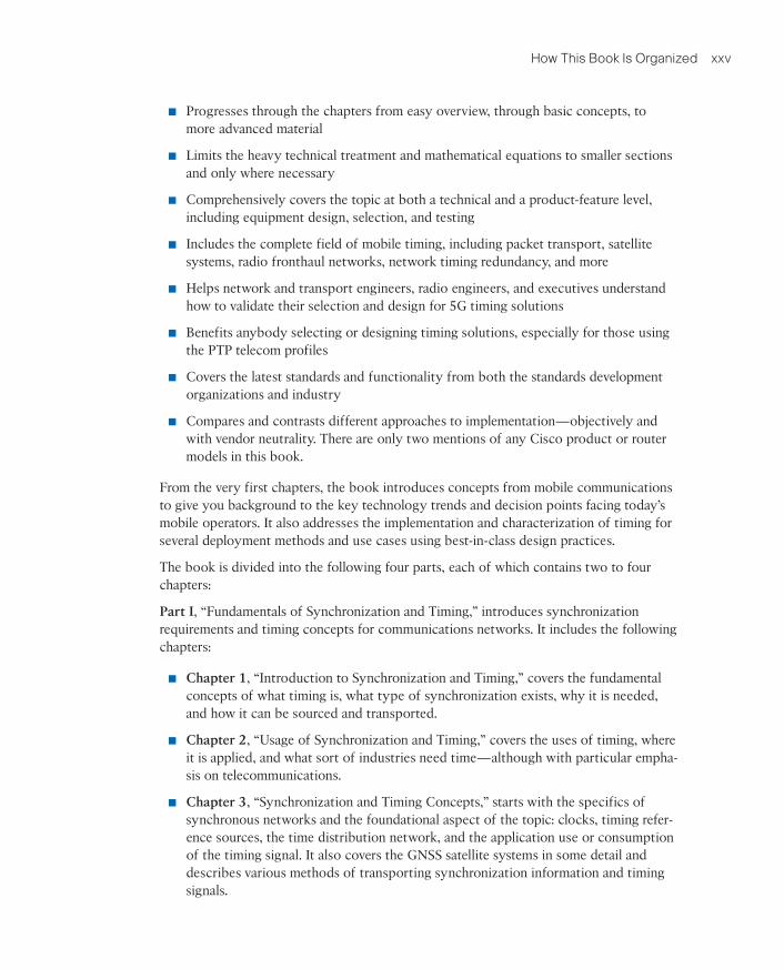
■■ Progresses through the chapters from easy overview, through basic concepts, to more advanced material
■■ Limits the heavy technical treatment and mathematical equations to smaller sections and only where necessary
■■ Comprehensively covers the topic at both a technical and a product-feature level, including equipment design, selection, and testing
■■ Includes the complete field of mobile timing, including packet transport, satellite systems, radio fronthaul networks, network timing redundancy, and more
■■ Helps network and transport engineers, radio engineers, and executives understand how to validate their selection and design for 5G timing solutions
■■ Benefits anybody selecting or designing timing solutions, especially for those using the PTP telecom profiles
■■ Covers the latest standards and functionality from both the standards development organizations and industry
■■ Compares and contrasts different approaches to implementation—objectively and with vendor neutrality. There are only two mentions of any Cisco product or router models in this book.
From the very first chapters, the book introduces concepts from mobile communications to give you background to the key technology trends and decision points facing today’s mobile operators. It also addresses the implementation and characterization of timing for several deployment methods and use cases using best-in-class design practices.
The book is divided into the following four parts, each of which contains two to four chapters:
Part I, “Fundamentals of Synchronization and Timing,” introduces synchronization requirements and timing concepts for communications networks. It includes the following chapters:
■■ Chapter 1, “Introduction to Synchronization and Timing,” covers the fundamental concepts of what timing is, what type of synchronization exists, why it is needed, and how it can be sourced and transported.
■■ Chapter 2, “Usage of Synchronization and Timing,” covers the uses of timing, where it is applied, and what sort of industries need time—although with particular empha-sis on telecommunications.
■■ Chapter 3, “Synchronization and Timing Concepts,” starts with the specifics of synchronous networks and the foundational aspect of the topic: clocks, timing refer-ence sources, the time distribution network, and the application use or consumption of the timing signal. It also covers the GNSS satellite systems in some detail and describes various methods of transporting synchronization information and timing signals.
9780136836254_print.indb 25 29/04/21 6:56 pm
xxvi Synchronizing 5G Mobile Networks
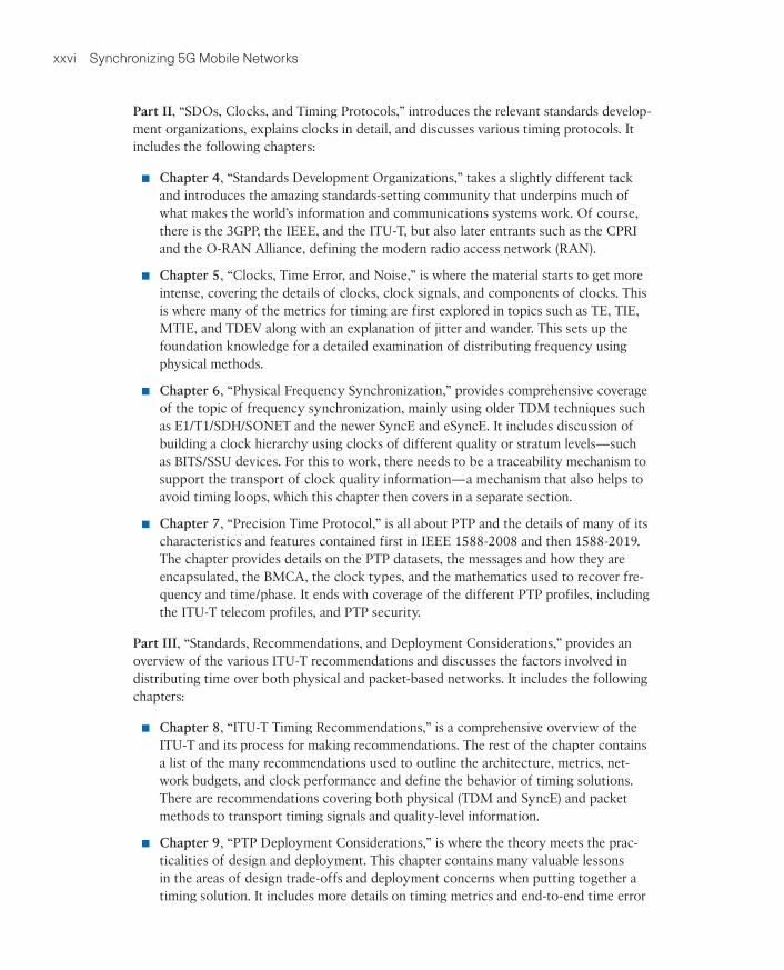
Part II, “SDOs, Clocks, and Timing Protocols,” introduces the relevant standards develop-ment organizations, explains clocks in detail, and discusses various timing protocols. It includes the following chapters:
■■ Chapter 4, “Standards Development Organizations,” takes a slightly different tack and introduces the amazing standards-setting community that underpins much of what makes the world’s information and communications systems work. Of course, there is the 3GPP, the IEEE, and the ITU-T, but also later entrants such as the CPRI and the O-RAN Alliance, defining the modern radio access network (RAN).
■■ Chapter 5, “Clocks, Time Error, and Noise,” is where the material starts to get more intense, covering the details of clocks, clock signals, and components of clocks. This is where many of the metrics for timing are first explored in topics such as TE, TIE, MTIE, and TDEV along with an explanation of jitter and wander. This sets up the foundation knowledge for a detailed examination of distributing frequency using physical methods.
■■ Chapter 6, “Physical Frequency Synchronization,” provides comprehensive coverage of the topic of frequency synchronization, mainly using older TDM techniques such as E1/T1/SDH/SONET and the newer SyncE and eSyncE. It includes discussion of building a clock hierarchy using clocks of different quality or stratum levels—such as BITS/SSU devices. For this to work, there needs to be a traceability mechanism to support the transport of clock quality information—a mechanism that also helps to avoid timing loops, which this chapter then covers in a separate section.
■■ Chapter 7, “Precision Time Protocol,” is all about PTP and the details of many of its characteristics and features contained first in IEEE 1588-2008 and then 1588-2019. The chapter provides details on the PTP datasets, the messages and how they are encapsulated, the BMCA, the clock types, and the mathematics used to recover fre-quency and time/phase. It ends with coverage of the different PTP profiles, including the ITU-T telecom profiles, and PTP security.
Part III, “Standards, Recommendations, and Deployment Considerations,” provides an overview of the various ITU-T recommendations and discusses the factors involved in distributing time over both physical and packet-based networks. It includes the following chapters:
■■ Chapter 8, “ITU-T Timing Recommendations,” is a comprehensive overview of the ITU-T and its process for making recommendations. The rest of the chapter contains a list of the many recommendations used to outline the architecture, metrics, net-work budgets, and clock performance and define the behavior of timing solutions. There are recommendations covering both physical (TDM and SyncE) and packet methods to transport timing signals and quality-level information.
■■ Chapter 9, “PTP Deployment Considerations,” is where the theory meets the prac-ticalities of design and deployment. This chapter contains many valuable lessons in the areas of design trade-offs and deployment concerns when putting together a timing solution. It includes more details on timing metrics and end-to-end time error
9780136836254_print.indb 26 29/04/21 6:56 pm
How This Book Is Organized xxvii
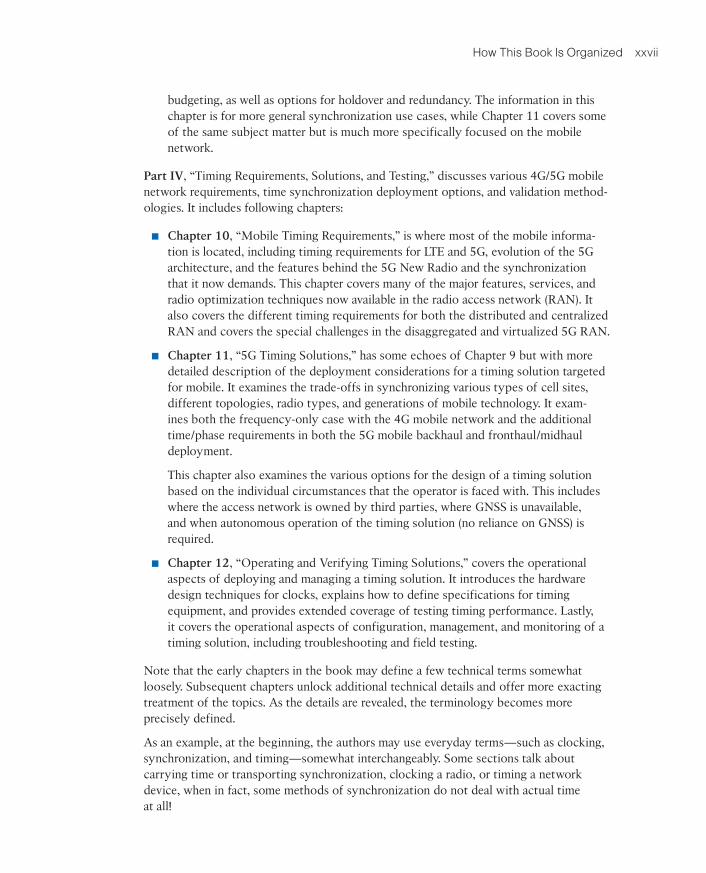
budgeting, as well as options for holdover and redundancy. The information in this chapter is for more general synchronization use cases, while Chapter 11 covers some of the same subject matter but is much more specifically focused on the mobile network.
Part IV, “Timing Requirements, Solutions, and Testing,” discusses various 4G/5G mobile network requirements, time synchronization deployment options, and validation method-ologies. It includes following chapters:
■■ Chapter 10, “Mobile Timing Requirements,” is where most of the mobile informa-tion is located, including timing requirements for LTE and 5G, evolution of the 5G architecture, and the features behind the 5G New Radio and the synchronization that it now demands. This chapter covers many of the major features, services, and radio optimization techniques now available in the radio access network (RAN). It also covers the different timing requirements for both the distributed and centralized RAN and covers the special challenges in the disaggregated and virtualized 5G RAN.
■■ Chapter 11, “5G Timing Solutions,” has some echoes of Chapter 9 but with more detailed description of the deployment considerations for a timing solution targeted for mobile. It examines the trade-offs in synchronizing various types of cell sites, different topologies, radio types, and generations of mobile technology. It exam-ines both the frequency-only case with the 4G mobile network and the additional time/phase requirements in both the 5G mobile backhaul and fronthaul/midhaul deployment.
■ This chapter also examines the various options for the design of a timing solution based on the individual circumstances that the operator is faced with. This includes where the access network is owned by third parties, where GNSS is unavailable, and when autonomous operation of the timing solution (no reliance on GNSS) is required.
■■ Chapter 12, “Operating and Verifying Timing Solutions,” covers the operational aspects of deploying and managing a timing solution. It introduces the hardware design techniques for clocks, explains how to define specifications for timing equipment, and provides extended coverage of testing timing performance. Lastly, it covers the operational aspects of configuration, management, and monitoring of a timing solution, including troubleshooting and field testing.
Note that the early chapters in the book may define a few technical terms somewhat loosely. Subsequent chapters unlock additional technical details and offer more exacting treatment of the topics. As the details are revealed, the terminology becomes more precisely defined.
As an example, at the beginning, the authors may use everyday terms—such as clocking, synchronization, and timing—somewhat interchangeably. Some sections talk about carrying time or transporting synchronization, clocking a radio, or timing a network device, when in fact, some methods of synchronization do not deal with actual time at all!
9780136836254_print.indb 27 29/04/21 6:56 pm
xxviii Synchronizing 5G Mobile Networks
The book does not give recommendations on which of these technologies should be deployed, nor does it provide a transition plan for a mobile operator. Each mobile operator can evaluate the technologies and make decisions based on their own criteria and circumstances. However, it does cover the details of the pros and cons behind each approach, allowing the engineer to make better-informed decisions.
We hope you enjoy reading and using this book as much as we enjoyed writing it!
9780136836254_print.indb 28 29/04/21 6:56 pm

In this chapter, you will learn the following:
■ Clocks: Covers clocks, clock signals, and the key components of clocks.
■ Time error: Explains what time error is, the different types of metrics to quantify time error, and how these metrics are useful in defining clock accuracy and stability.
■ Holdover performance: Explains holdover for clocks, applicable whenever a synchronization reference is temporarily lost, and why the holdover capability of a clock becomes critical to ensure optimal network and application functioning.
■ Transient response: Examines what happens when a slave clock changes its input reference.
■ Measuring time error: Describes how to determine and quantify the key metrics of time error.
In earlier chapters, you read that any clock can only be near perfect (none are perfect)—there are always inherent errors in clocks. In this chapter, you will discover the various components of a clock and understand how these components contribute to removing or introducing certain errors. Because these errors can adversely impact the consumer of the synchronization services (the end application), it is important to track and quantify them. Once measured, these errors are compared against some defined performance parameters to determine how much (if any) impact they have on the end application. This chapter also explains the different metrics used to quantify time error and how to measure them.
ClocksIn everyday usage, the term clock refers to a device that maintains and displays the time of day and perhaps the date. In the world of electronics, however, clock refers to a micro-chip that generates a clock signal, which is used to regulate the timing and speed of the components on a circuit board. This clock signal is a waveform that is generated either by
Clocks, Time Error, and Noise
Chapter 5
9780136836254_print.indb 139 29/04/21 6:57 pm
140 Chapter 5: Clocks, Time Error, and Noise
a clock generator or the clock itself—the most common form of clock signal in electron-ics is a square wave.
This type of clock is able to generate clock signals of different frequencies and phases as may be required by separate components within an electronic circuit or device. The fol-lowing are some examples showing the functions of a clock:
■ Most sophisticated electronic devices require a clock signal for proper operation. These devices require that the clock signal delivered to them adheres to a core set of specifications.
■ All electronics devices on an electronic circuit board communicate with each other to accomplish certain tasks. Every device might require clock signals with a different specification; providing the needed signals allows these devices to interoperate with each other.
In both cases, a clock device on the circuit board provides such signals.
Note Use of the terms “master” and “slave” is ONLY in association with the official ter-minology used in industry specifications and standards, and in no way diminishes Pearson’s commitment to promoting diversity, equity, and inclusion, and challenging, countering and/or combating bias and stereotyping in the global population of the learners we serve.
When discussing network synchronization or designing a timing distribution network, the timing signals need to travel much further than a circuit board. In this case, nodes must transfer clock signal information across the network. To achieve this, the engineer designates a clock as either a master clock or a slave clock. The master clock is the source for the clock signals, and a slave clock then synchronizes or aligns its clock signals to that of the master.
A clock signal relates to a (hardware) clock subsystem that generates a clocking signal, but often engineers refer to it simply using the term clock. You might hear the statement, “the clock on node A is not synchronized to a reference clock,” whereas the real meaning of clock in this sentence is that the clock signals are not synchronized. So, clock signal and clock are technically different terms with different meanings, but because the com-mon usage has made one refer to the other, this chapter will also use the term clock to refer to a clock signal.
Oscillators
An electronic oscillator is a device that “oscillates” when an electric current is applied to it, causing the device to generate a periodic and continuous waveform. This waveform can be of different wave shapes and frequencies, but for most purposes, the clock signals utilized are sine waves or square waves. Thus, oscillators are a simple form of clock signal generation device.
9780136836254_print.indb 140 29/04/21 6:57 pm
Clocks 141
There are a few different types of oscillators (as described in Chapter 3, “Synchronization and Timing Concepts”), but in modern electronics, crystal oscillators (referred to as XO) are the most common. The crystal oscillator is made up of a special type of crystal, which is piezoelectric in nature, which means that when electric current is applied to this crystal, it oscillates and emits a signal at a very specific frequency. The frequency could vary from a few tens of kHz to hundreds of MHz depending on the physical properties of the crystal.
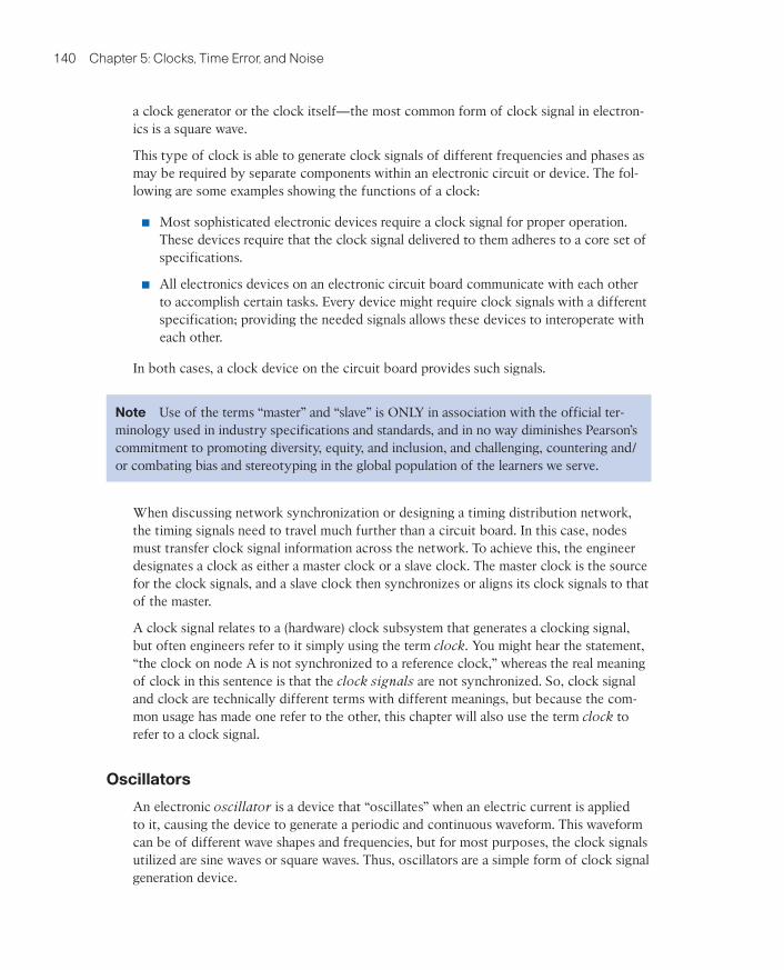
Quartz is one example of a piezoelectric crystal and is commonly used in many consumer devices, such as wristwatches, wall clocks, and computers. Similar devices are also used in networking devices such as switches, routers, radio base stations, and so on. Figure 5-1 shows a typical crystal commonly utilized in such a device.
Figure 5-1 16-MHz Crystal Oscillator
The quartz that is being used in crystal oscillators is a naturally occurring element, although manufacturers grow their own for purity. The natural frequency of the clock signal generated by a crystal depends on the shape or physical properties (sometimes referred to as the cut) of the crystal.
On the other hand, the stability of the output signal is also heavily influenced by many environmental factors, such as temperature, humidity, pressure, vibration, and magnetic and electric fields. Engineers refer to this as the sensitivity of the oscillator to environ-mental factors. For a given oscillator, the sensitivity to one factor is often dependent on the sensitivity to another factor, as well as the age of the crystal or device itself.
As a real-life example, if your wristwatch is using a 32,768-Hz quartz crystal oscillator, the accuracy of the wristwatch in different environmental conditions will vary. The same behavior also applies to other electronic equipment, including transport devices and routers in the network infrastructure. This means that when electronic devices are used to synchronize devices to a common frequency, phase, or time, the environmental condi-tions adversely impact the stability of synchronization.
M05_Hagarty_CH05_p139-178.indd 141 30/04/21 8:19 pm
142 Chapter 5: Clocks, Time Error, and Noise
Note The accuracy for wristwatches is usually measured in seconds or minutes, while for other tasks involving network transport, the accuracy requirement is frequently small frac-tions of a second—microseconds (millionths of a second) or even nanoseconds (billionths of a second).
There have been many innovations to improve the stability of crystal oscillators deployed in unstable environmental conditions. One common approach in modern designs is for the hardware designer to design a circuit to vary the voltage being applied to the oscil-lator to adjust its frequency in small amounts. This class of crystal oscillator is known as voltage-controlled crystal oscillators (VCXO).
Of the many environmental factors that affect the stability and accuracy of a crystal oscillator, the major one is temperature. To provide better oscillator stability of crystal against temperature variations, two additional types of oscillators have emerged in the market:
■ Temperature-compensated crystal oscillators (TCXO) are crystal oscillators designed to provide improved frequency stability despite wide variations in tem-perature. TCXOs have a temperature compensation circuit together with the crystal, which measures the ambient temperature and compensates for any change by alter-ing the voltage applied to the crystal. By aligning the voltage to values within the possible temperature range, the compensation circuit stabilizes the output clock frequency at different temperatures.
■ Oven-controlled crystal oscillators (OCXO) are crystal oscillators where the crys-tal itself is placed in an oven that attempts to maintain a specific temperature inside the crystal housing, independent of the temperature changes occurring outside. This reduces the temperature variation on the oscillator and thereby increases the stability of the frequency. As you can imagine, oscillators with additional heating compo-nents end up bulkier and costlier than TCXOs.
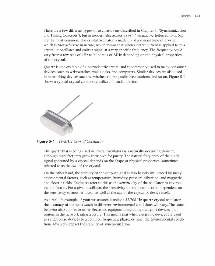
The basic approach with the TCXO is to compensate for measured changes in tempera-ture by applying appropriate changes in voltage, whereas for the OCXO, the tempera-ture is controlled (by being elevated above the expected operating temperature range). Figure 5-2 shows a typical OCXO.
An oscillator is the core component of a clock, which alone can significantly impact the quality of the clock. An approximate comparison of stability between these different oscillators suggests that the stability of an OCXO might be 10 to 100 times higher than a TCXO class device. Table 3-2 in Chapter 3 outlines the characteristics of the common types of oscillator.
The stability of an oscillator type also gets reflected in the cost. As a very rough esti-mate, cesium-based oscillators cost about $50,000 and rubidium-based oscillators around $100, whereas an OCXO costs around $30 and a TCXO would be less than $10.
9780136836254_print.indb 142 29/04/21 6:57 pm
Clocks 143
Figure 5-2 Typical OCXO
PLLs
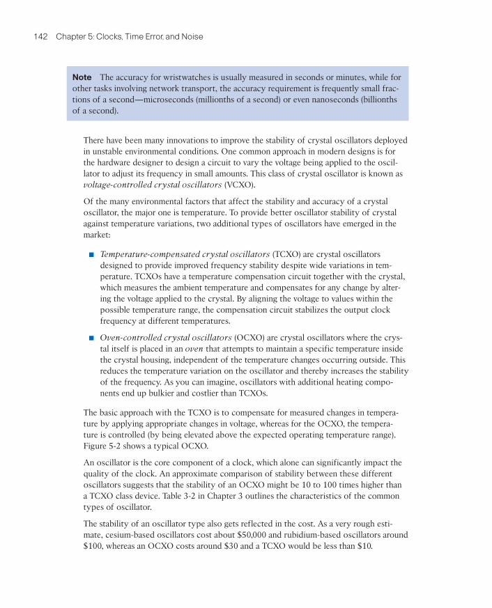
A phase-locked loop (PLL) is an electronic device or circuit that generates an output clock signal that is phase-aligned as well as frequency-aligned to an input clock signal. As shown in Figure 5-3, in its simplest form, a PLL circuit consists of three basic elements, as described in the list that follows.
Input clock signal Phase comparator Loop filter VCOOutputsignal
Basic block diagram of PLL
Figure 5-3 PLL Building Blocks
■ Voltage-controlled oscillator (VCO): A special type of oscillator that changes frequency with changes in an input voltage (in this case from the loop filter). The frequency of the VCO with a nominal control signal applied is called the free- running frequency, indicated by the symbol f0.
■ Phase comparator: Compares the phase of two signals (input clock and local oscil-lator) and generates a voltage according to the phase difference detected between the two signals. This output voltage is fed into the loop filter.
M05_Hagarty_CH05_p139-178.indd 143 30/04/21 8:20 pm
144 Chapter 5: Clocks, Time Error, and Noise
■ PLL loop filter: Primary function is to detect and filter out undesired phase changes passed on by the phase comparator in the form of voltage. This filtered voltage is then applied to the VCO to adjust the frequency. It is important to note that if the voltage is not filtered appropriately, it will result in a signal that exactly follows the input clock, inheriting all the variations or errors of the input clock reference. Thus, the properties of the loop filter directly affect the stability and performance of a PLL and the quality of the output signal.
When a PLL is initially turned on, the VCO with a nominal control signal applied will provide its free-running frequency (f0). When fed an input signal, the phase compara-tor measures the phase difference compared to the VCO signal. Based on the size of the phase difference between the two signals, the phase comparator generates a correcting voltage and feeds it to the loop filter.
The loop filter removes (or filters out) the noise and passes the filtered voltage to the VCO. With the new voltage applied, the VCO output frequency begins to change. Assuming the input signal and VCO frequency are not the same, the phase comparator sees this as a phase shift, and the output of the loop filter will be an increasing or decreasing voltage depending on which signal has higher frequency.
This voltage adjustment causes the VCO to continuously change its frequency, reducing the difference between VCO and input frequency. Eventually the size of changes in the output voltage of the loop filter are also reduced, resulting in ever smaller changes to the VCO frequency—at some point achieving a “locked” state.
Any further change in input or VCO frequency is also tracked by a change in loop filter output, keeping the two frequencies very closely aligned. This process continues as long as an input signal is detected. The filtering process is covered in detail in the following section in this chapter.
Recall that the input signal, even one generated from a very stable source (such as an atomic clock), would have accumulated noise (errors) on its journey over the clocking chain. The main purpose of a PLL is to align frequency (and phase) to the long-term average of the input signal and ignore (filter out) short-term changes.
Now a couple of questions arise:
■ Will the loop filter react and vary the voltage fed to the VCO for every phase variation seen on the input signal?
■ When should the PLL declare itself in locked state or, conversely, if already in locked state, under what conditions could the PLL declare that it has lost its lock with the input reference?
The first question raised is answered in the next section, but the second question needs a discussion on PLL states and the regions of operation of a PLL. The PLL is said to be in the transient state when the output is not locked to the input reference and it is in the
9780136836254_print.indb 144 29/04/21 6:57 pm
Clocks 145
process of locking to the input signal. Alternatively, the steady state is when the PLL is locked with the input reference. As explained earlier, even during steady-state operations, the VCO will keep adjusting the frequency to match the input frequency based on the differential voltage being fed from the loop filter.
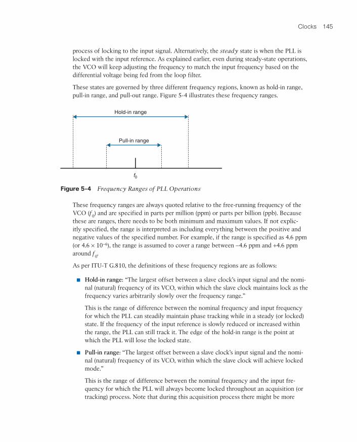
These states are governed by three different frequency regions, known as hold-in range, pull-in range, and pull-out range. Figure 5-4 illustrates these frequency ranges.
Hold-in range
Pull-in range
f0
Figure 5-4 Frequency Ranges of PLL Operations
These frequency ranges are always quoted relative to the free-running frequency of the VCO (f0) and are specified in parts per million (ppm) or parts per billion (ppb). Because these are ranges, there needs to be both minimum and maximum values. If not explic-itly specified, the range is interpreted as including everything between the positive and negative values of the specified number. For example, if the range is specified as 4.6 ppm (or 4.6 × 10⁻⁶), the range is assumed to cover a range between -4.6 ppm and +4.6 ppm around f0.
As per ITU-T G.810, the definitions of these frequency regions are as follows:
■ Hold-in range: “The largest offset between a slave clock’s input signal and the nomi-nal (natural) frequency of its VCO, within which the slave clock maintains lock as the frequency varies arbitrarily slowly over the frequency range.”
This is the range of difference between the nominal frequency and input frequency for which the PLL can steadily maintain phase tracking while in a steady (or locked) state. If the frequency of the input reference is slowly reduced or increased within the range, the PLL can still track it. The edge of the hold-in range is the point at which the PLL will lose the locked state.
■ Pull-in range: “The largest offset between a slave clock’s input signal and the nomi-nal (natural) frequency of its VCO, within which the slave clock will achieve locked mode.”
This is the range of difference between the nominal frequency and the input fre-quency for which the PLL will always become locked throughout an acquisition (or tracking) process. Note that during this acquisition process there might be more
9780136836254_print.indb 145 29/04/21 6:57 pm
146 Chapter 5: Clocks, Time Error, and Noise
than one cycle slip, but the PLL will always lock to the input signal. This is the range of frequencies within which a PLL can transition from the transient state to steady (locked) state.
■ Pull-out range: “The offset between a slave clock’s input signal and the nominal (nat-ural) frequency of its VCO, within which the slave clock stays in the locked mode and outside of which the slave clock cannot maintain locked mode, irrespective of the rate of the frequency change.”
This can be seen as the range of the frequency step, which if applied to a steady-state PLL, the PLL still remains in the steady (or locked) state. The PLL declares itself not locked if the input frequency step is outside of this range.
Taking an example from ITU-T G.812, both the pull-in and hold-in ranges for Type III clock type is defined as 4.6 × 10⁻⁶, which is the same as ±4.6 ppm. Table 3-3 in Chapter 3 provides a quick reference of these frequency ranges for different types of clock nodes.
When the PLL is tracking an input reference, it is the loop filter that is enforcing the limits of these frequency ranges. The loop filter is usually a low-pass filter, and as the name suggests, it allows only low-frequency (slow) variations to pass through. That means it removes high-frequency variation and noise in the reference signal. Conversely, a high-pass filter allows high-frequency variations to pass and removes the low-frequency changes.
While these filters are discussed in the next section in detail, it is important to note that “low-frequency variations” does not refer to the frequency of the clock signal, but the rate with which the frequency or phase of the clock signal varies. Low rate (less frequent) changes are a gradual wander in the signal, whereas high rate changes are a very short-term jitter in the signal. You will read more about jitter and wander later in this chapter.
Because PLLs synchronize local clock signals to an external or reference clock signal, these devices have become one of the most commonly used electronic circuits on any communication device. Out of several types of PLL devices, one of the main types of PLL used today is the digital PLL (DPLL), which is used to synchronize digital signals.
It is worthwhile noting that, just like any other electronic circuits and devices, PLLs have also been evolving. Designers of modern communications equipment are incorporating the latest PLL devices into them, circuits that now contain multiple PLLs (analogue or digital).
To reduce real-estate requirements on circuit boards, newer-generation devices can oper-ate with lower-frequency oscillators that can replace expensive high-frequency oscilla-tors. They also output signals with ultra-low levels of jitter that is required for the tight jitter specifications required by some equipment designs (remembering that jitter is high-frequency noise).
9780136836254_print.indb 146 29/04/21 6:57 pm
Clocks 147
Low-Pass and High-Pass Filters
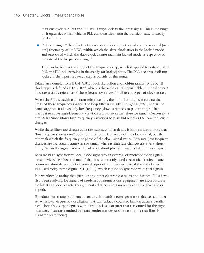
A low-pass filter (LPF) is a filter that filters out (removes) signals that are higher than a fixed frequency, which means an LPF passes only signals that are lower than a certain frequency—hence the name low-pass filter. For the same reasons, sometimes LPFs are also called high-cut filters because they cut off signals higher than some fixed frequency. Figure 5-5 illustrates LPF filtering where signals with lower frequency than a cut-off frequency are not attenuated (diminished). The pass band is the range of frequencies that are not attenuated, and the stop band is the range of frequencies that are attenuated.
Meanwhile, the range up to the cut-off frequency becomes the clock bandwidth, which also matches the width of a filter’s pass band. For example, as shown in Figure 5-5, in the case of an LPF, the clock bandwidth is the range of frequencies that constitute the pass band. The clock bandwidth is typically a configurable parameter based on the capabili-ties of a PLL.
Stop bandPass band
Cut-off frequency
Frequency
Bandwidth
Figure 5-5 Low-Pass Filter
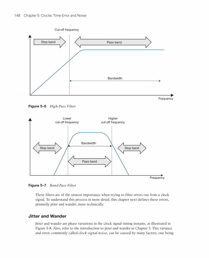
Similarly, a high-pass filter (HPF) is a device that filters out signals that are lower than some fixed frequency, which means that an HPF passes only signals that are higher than a certain frequency. And again, HPFs are also sometimes called low-cut filters because they cut off lower than a fixed frequency signal. Figure 5-6 depicts an HPF, showing that the pass band and stop band are a mirror image of the LPF case.
It is interesting to note that combining both filters (LPF and HPF) on a circuit, you could design a system to allow only a certain range of frequencies and filter out the rest. Such a combination of LPF and HPF behaves as shown in Figure 5-7 and is called a band-pass filter. The band-pass name comes from the fact that it allows a certain band of frequen-cies (from lower cut-off to higher cut-off) to pass and attenuates the rest of the spectrum.
9780136836254_print.indb 147 29/04/21 6:57 pm
148 Chapter 5: Clocks, Time Error, and Noise
Pass bandStop band
Bandwidth
Frequency
Cut-off frequency
Figure 5-6 High-Pass Filter
Bandwidth
Highercut-off frequency
Lowercut-off frequency
Stop band Stop band
Pass band
Frequency
Figure 5-7 Band-Pass Filter
These filters are of the utmost importance when trying to filter errors out from a clock signal. To understand this process in more detail, this chapter next defines these errors, primarily jitter and wander, more technically.
Jitter and Wander
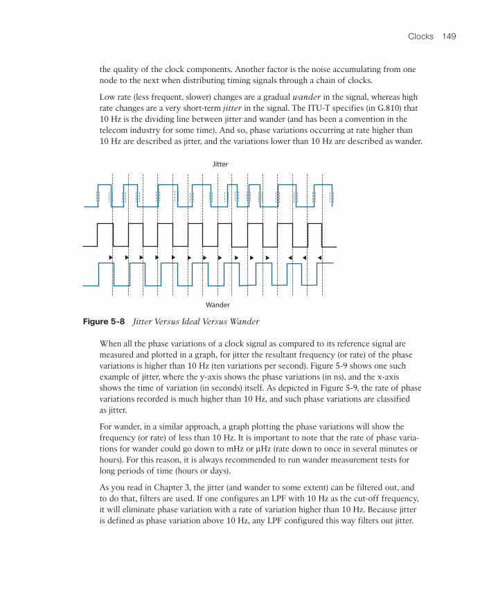
Jitter and wander are phase variations in the clock signal timing instants, as illustrated in Figure 5-8. Also, refer to the introduction to jitter and wander in Chapter 3. This variance and error, commonly called clock signal noise, can be caused by many factors, one being
9780136836254_print.indb 148 29/04/21 6:57 pm
Clocks 149
the quality of the clock components. Another factor is the noise accumulating from one node to the next when distributing timing signals through a chain of clocks.
Low rate (less frequent, slower) changes are a gradual wander in the signal, whereas high rate changes are a very short-term jitter in the signal. The ITU-T specifies (in G.810) that 10 Hz is the dividing line between jitter and wander (and has been a convention in the telecom industry for some time). And so, phase variations occurring at rate higher than 10 Hz are described as jitter, and the variations lower than 10 Hz are described as wander.
Jitter
Wander
Figure 5-8 Jitter Versus Ideal Versus Wander
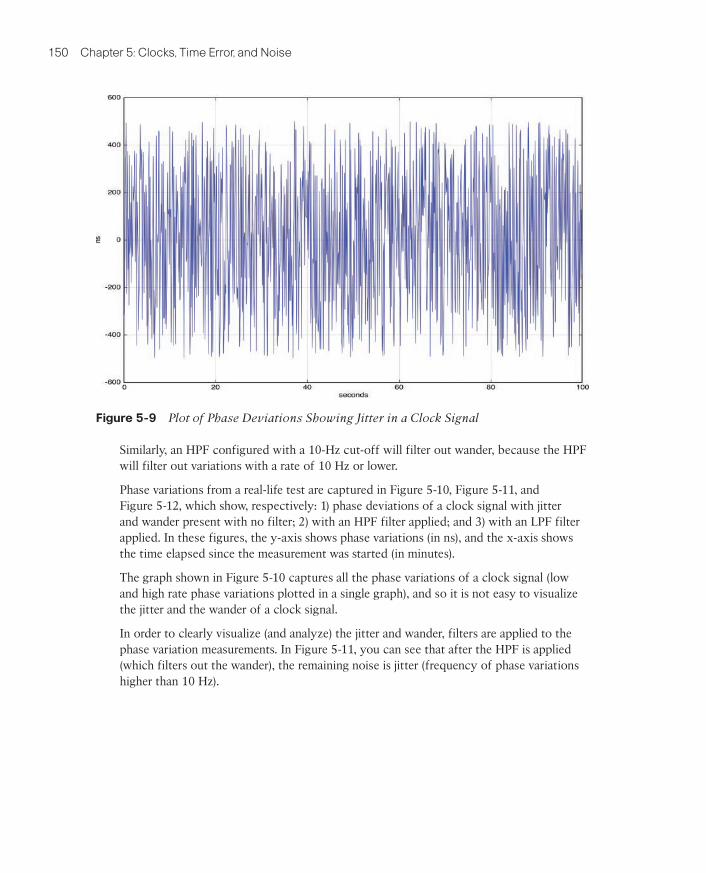
When all the phase variations of a clock signal as compared to its reference signal are measured and plotted in a graph, for jitter the resultant frequency (or rate) of the phase variations is higher than 10 Hz (ten variations per second). Figure 5-9 shows one such example of jitter, where the y-axis shows the phase variations (in ns), and the x-axis shows the time of variation (in seconds) itself. As depicted in Figure 5-9, the rate of phase variations recorded is much higher than 10 Hz, and such phase variations are classified as jitter.
For wander, in a similar approach, a graph plotting the phase variations will show the frequency (or rate) of less than 10 Hz. It is important to note that the rate of phase varia-tions for wander could go down to mHz or µHz (rate down to once in several minutes or hours). For this reason, it is always recommended to run wander measurement tests for long periods of time (hours or days).
As you read in Chapter 3, the jitter (and wander to some extent) can be filtered out, and to do that, filters are used. If one configures an LPF with 10 Hz as the cut-off frequency, it will eliminate phase variation with a rate of variation higher than 10 Hz. Because jitter is defined as phase variation above 10 Hz, any LPF configured this way filters out jitter.
9780136836254_print.indb 149 29/04/21 6:57 pm
150 Chapter 5: Clocks, Time Error, and Noise
Figure 5-9 Plot of Phase Deviations Showing Jitter in a Clock Signal
Similarly, an HPF configured with a 10-Hz cut-off will filter out wander, because the HPF will filter out variations with a rate of 10 Hz or lower.
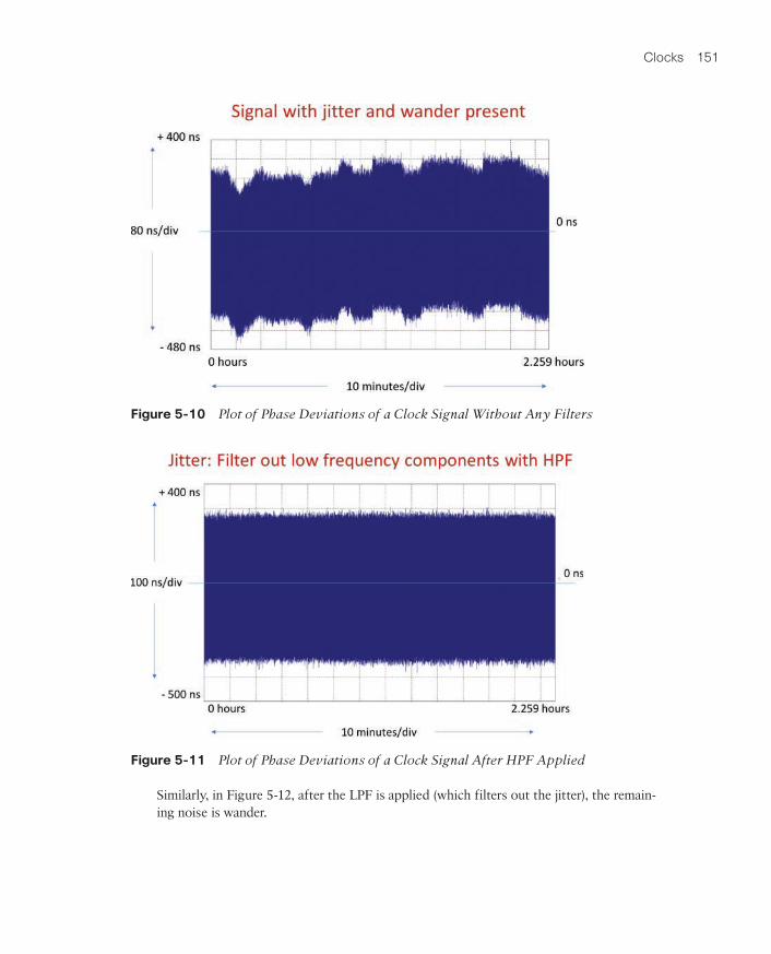
Phase variations from a real-life test are captured in Figure 5-10, Figure 5-11, and Figure 5-12, which show, respectively: 1) phase deviations of a clock signal with jitter and wander present with no filter; 2) with an HPF filter applied; and 3) with an LPF filter applied. In these figures, the y-axis shows phase variations (in ns), and the x-axis shows the time elapsed since the measurement was started (in minutes).
The graph shown in Figure 5-10 captures all the phase variations of a clock signal (low and high rate phase variations plotted in a single graph), and so it is not easy to visualize the jitter and the wander of a clock signal.
In order to clearly visualize (and analyze) the jitter and wander, filters are applied to the phase variation measurements. In Figure 5-11, you can see that after the HPF is applied (which filters out the wander), the remaining noise is jitter (frequency of phase variations higher than 10 Hz).
9780136836254_print.indb 150 29/04/21 6:57 pm
Clocks 151
Figure 5-10 Plot of Phase Deviations of a Clock Signal Without Any Filters
Figure 5-11 Plot of Phase Deviations of a Clock Signal After HPF Applied
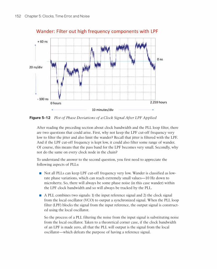
Similarly, in Figure 5-12, after the LPF is applied (which filters out the jitter), the remain-ing noise is wander.
9780136836254_print.indb 151 29/04/21 6:57 pm
152 Chapter 5: Clocks, Time Error, and Noise
Figure 5-12 Plot of Phase Deviations of a Clock Signal After LPF Applied
After reading the preceding section about clock bandwidth and the PLL loop filter, there are two questions that could arise. First, why not keep the LPF cut-off frequency very low to filter the jitter and also limit the wander? Recall that jitter is filtered with the LPF. And if the LPF cut-off frequency is kept low, it could also filter some range of wander. Of course, this means that the pass band for the LPF becomes very small. Secondly, why not do the same on every clock node in the chain?
To understand the answer to the second question, you first need to appreciate the following aspects of PLLs:
■ Not all PLLs can keep LPF cut-off frequency very low. Wander is classified as low-rate phase variations, which can reach extremely small values—10 Hz down to microhertz. So, there will always be some phase noise (in this case wander) within the LPF clock bandwidth and so will always be tracked by the PLL.
■ A PLL combines two signals: 1) the input reference signal and 2) the clock signal from the local oscillator (VCO) to output a synchronized signal. When the PLL loop filter (LPF) blocks the signal from the input reference, the output signal is construct-ed using the local oscillator.
So the process of a PLL filtering the noise from the input signal is substituting noise from the local oscillator. Taken to a theoretical corner case, if the clock bandwidth of an LPF is made zero, all that the PLL will output is the signal from the local oscillator—which defeats the purpose of having a reference signal.
9780136836254_print.indb 152 29/04/21 6:57 pm
Clocks 153
So, if using a very low cut-off frequency for the LPF, the PLL needs to be matched to a good-quality local oscillator, so that the noise added by the local oscillator is reduced. For the hardware designer, this has obvious cost ramifications—to get bet-ter noise filtering, you need to spend more money on the oscillator.
■ The time taken for a PLL to move from transient state to the steady (or locked) state depends on the clock bandwidth (as well as the input frequency and quality of the local oscillator). The narrower the clock bandwidth for the LPF, the longer time it takes for the PLL to move to the steady state.
For example, a synchronization supply unit (SSU) type I clock or building integrated timing supply (BITS) stratum 2 clock with an LPF configured for bandwidth of 3 mHz will take several minutes to lock to an input signal. However, telecom net-works are very widely distributed and can consist of long chains of clock nodes. If all the clocks in the chain had low bandwidth, the complete chain could take many hours to settle to a steady state. Similarly, it might take several hours for the last node of the chain to settle down after any disruption to the distribution of clock.
It is for these reasons that a clock node with better filtering capabilities should have a good-quality oscillator and should be placed in a chain of clock nodes at selected locations. These factors also explain why SSU/BITS clock nodes (which have stratum 2– quality oscillators and better PLL capabilities) are recommended only after a certain number of SDH equipment clock (SEC) nodes. The section “Synchronization Network Chain” in Chapter 6, “Physical Frequency Synchronization,” covers this limit and recom-mendations by ITU-T in greater detail.
To ensure interoperability between devices and to minimize the signal degradation due to jitter and wander accumulation across the network, the ITU-T recommendations (such as G.8261 and G.8262) specify jitter and wander performance limits for networks and clocks. The normal network elements (NE) and synchronous Ethernet equipment clocks (EEC) are usually allocated the most relaxed limits.
For example, ITU-T G.8262 specifies the maximum amount of peak-to-peak output jitter (within a defined bandwidth) permitted from an EEC. This is to ensure that the amount of jitter never exceeds the specified input tolerance level for subsequent EECs. Chapter 8, “ITU-T Timing Recommendations,” covers the ITU-T recommendations in greater detail.
Frequency Error
While jitter and wander are both metrics to measure phase errors, the frequency error (or accuracy) also needs to be measured.
The frequency error (also referred to as frequency accuracy) is the degree to which the frequency of a clock can deviate from a nominal (or reference) frequency. The metric to measure this degree is called the fractional frequency deviation (FFD) or sometimes just the frequency offset. This offset is also referred to as the fractional frequency offset (FFO).
9780136836254_print.indb 153 29/04/21 6:57 pm
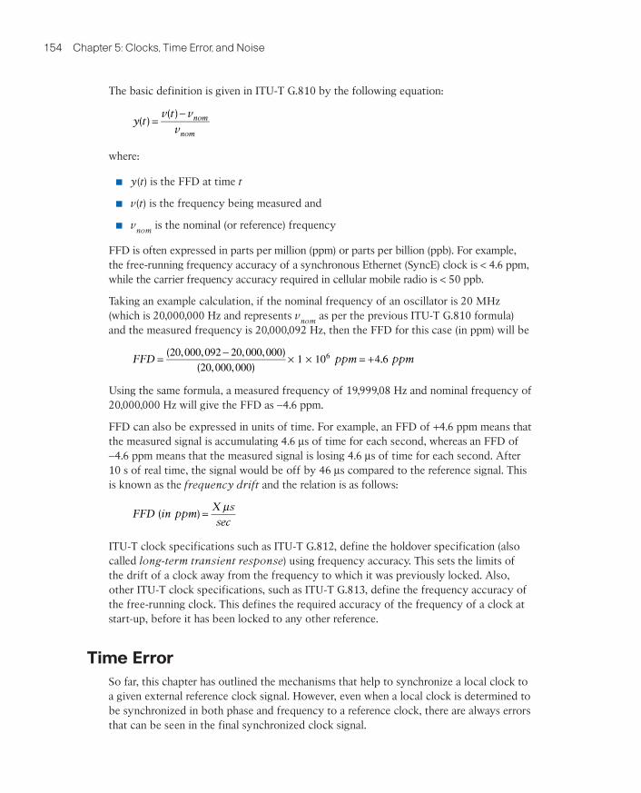
154 Chapter 5: Clocks, Time Error, and Noise
The basic definition is given in ITU-T G.810 by the following equation:
y tv t v
vnom
nom( )
( )=
−
where:
■ y(t) is the FFD at time t
■ v(t) is the frequency being measured and
■ vnom is the nominal (or reference) frequency
FFD is often expressed in parts per million (ppm) or parts per billion (ppb). For example, the free-running frequency accuracy of a synchronous Ethernet (SyncE) clock is < 4.6 ppm, while the carrier frequency accuracy required in cellular mobile radio is < 50 ppb.
Taking an example calculation, if the nominal frequency of an oscillator is 20 MHz (which is 20,000,000 Hz and represents vnom as per the previous ITU-T G.810 formula) and the measured frequency is 20,000,092 Hz, then the FFD for this case (in ppm) will be
FFD ppm ppm( , , , , )
( , , ).20 000 092 20 000 000
20 000 0001 10 4 66= − × × = +
Using the same formula, a measured frequency of 19,999,08 Hz and nominal frequency of 20,000,000 Hz will give the FFD as -4.6 ppm.
FFD can also be expressed in units of time. For example, an FFD of +4.6 ppm means that the measured signal is accumulating 4.6 µs of time for each second, whereas an FFD of -4.6 ppm means that the measured signal is losing 4.6 µs of time for each second. After 10 s of real time, the signal would be off by 46 µs compared to the reference signal. This is known as the frequency drift and the relation is as follows:
FFD in ppmX ssec
( ) µ=
ITU-T clock specifications such as ITU-T G.812, define the holdover specification (also called long-term transient response) using frequency accuracy. This sets the limits of the drift of a clock away from the frequency to which it was previously locked. Also, other ITU-T clock specifications, such as ITU-T G.813, define the frequency accuracy of the free-running clock. This defines the required accuracy of the frequency of a clock at start-up, before it has been locked to any other reference.
Time ErrorSo far, this chapter has outlined the mechanisms that help to synchronize a local clock to a given external reference clock signal. However, even when a local clock is determined to be synchronized in both phase and frequency to a reference clock, there are always errors that can be seen in the final synchronized clock signal.
9780136836254_print.indb 154 29/04/21 6:57 pm
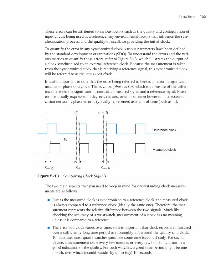
Time Error 155
These errors can be attributed to various factors such as the quality and configuration of input circuit being used as a reference; any environmental factors that influence the syn-chronization process; and the quality of oscillator providing the initial clock.
To quantify the error in any synchronized clock, various parameters have been defined by the standard development organizations (SDO). To understand the errors and the vari-ous metrics to quantify these errors, refer to Figure 5-13, which illustrates the output of a clock synchronized to an external reference clock. Because the measurement is taken from the synchronized clock that is receiving a reference signal, this synchronized clock will be referred to as the measured clock.
It is also important to note that the error being referred to here is an error in significant instants or phase of a clock. This is called phase error, which is a measure of the differ-ence between the significant instants of a measured signal and a reference signal. Phase error is usually expressed in degrees, radians, or units of time; however, in telecommuni-cation networks, phase error is typically represented as a unit of time (such as ns).
x(n - 1)
Tc
(n) (n + 1)
x(n + 1)x(n)
Reference clock
Measured clock
Figure 5-13 Comparing Clock Signals
The two main aspects that you need to keep in mind for understanding clock measure-ments are as follows:
■ Just as the measured clock is synchronized to a reference clock, the measured clock is always compared to a reference clock (ideally the same one). Therefore, the mea-surement represents the relative difference between the two signals. Much like checking the accuracy of a wristwatch, measurement of a clock has no meaning unless it is compared to a reference.
■ The error in a clock varies over time, so it is important that clock errors are measured over a sufficiently long time period to thoroughly understand the quality of a clock. To illustrate, most quartz watches gain/lose some time (seconds) daily. For such a device, a measurement done every few minutes or every few hours might not be a good indication of the quality. For such watches, a good time period might be one month, over which it could wander by up to (say) 10 seconds.
9780136836254_print.indb 155 29/04/21 6:57 pm
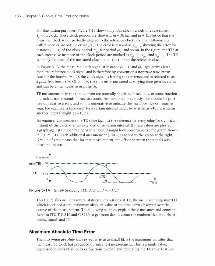
156 Chapter 5: Clocks, Time Error, and Noise
For illustration purposes, Figure 5-13 shows only four clock periods or cycle times, Tc, of a clock. These clock periods are shown as (n - 1), (n), and (n + 1). Notice that the measured clock is not perfectly aligned to the reference clock, and that difference is called clock error or time error (TE). The error is marked as x(n - 1) showing the error for instance (n - 1) of the clock period, x(n) for period (n), and so on. In the figure, the TEs at each successive instance of the clock period are marked as x(n - 1), x(n), and x(n + 1). The TE is simply the time of the measured clock minus the time of the reference clock.
In Figure 5-13, the measured clock signal at instance (n - 1) and (n) lags (arrives later than) the reference clock signal and is therefore by convention a negative time error. And for the interval (n + 1), the clock signal is leading the reference and is referred to as a positive time error. Of course, the time error measured at varying time periods varies and can be either negative or positive.
TE measurements in the time domain are normally specified in seconds, or some fraction of, such as nanoseconds or microseconds. As mentioned previously, there could be posi-tive or negative errors, and so it is imperative to indicate this via a positive or negative sign. For example, a time error for a certain interval might be written as +40 ns, whereas another interval might be -10 ns.
An engineer can measure the TE value (against the reference) at every edge (or significant instant) of the clock over an extended observation interval. If these values are plotted in a graph against time on the horizontal axis, it might look something like the graph shown in Figure 5-14. Each additional measurement (+ or -) is added to the graph at the right. A value of zero means that for that measurement, the offset between the signals was measured as zero.
Time error
Time
max|TE|
cTEdTE
50ns
15 ns
0
Figure 5-14 Graph Showing cTE, dTE, and max|TE|
This figure also includes several statistical derivations of TE, the main one being max|TE|, which is defined as the maximum absolute value of the time error observed over the course of the measurement. The following sections explain these measures and concepts. Refer to ITU-T G.810 and G.8260 to get more details about the mathematical models of timing signals and TE.
Maximum Absolute Time Error
The maximum absolute time error, written as max|TE|, is the maximum TE value that the measured clock has produced during a test measurement. This is a single value, expressed in units of seconds or fractions thereof, and represents the TE value that lies
9780136836254_print.indb 156 29/04/21 6:57 pm
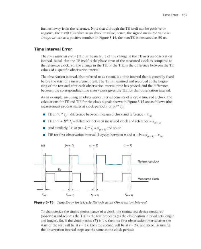
Time Error 157
furthest away from the reference. Note that although the TE itself can be positive or negative, the max|TE| is taken as an absolute value; hence, the signed measured value is always written as a positive number. In Figure 5-14, the max|TE| is measured as 50 ns.
Time Interval Error
The time interval error (TIE) is the measure of the change in the TE over an observation interval. Recall that the TE itself is the phase error of the measured clock as compared to the reference clock. So, the change in the TE, or the TIE, is the difference between the TE values of a specific observation interval.
The observation interval, also referred to as τ (tau), is a time interval that is generally fixed before the start of a measurement test. The TE is measured and recorded at the begin-ning of the test and after each observation interval time has passed; and the difference between the corresponding time error values gives the TIE for that observation interval.
As an example, assuming an observation interval consists of k cycle times of a clock, the calculations for TE and TIE for the clock signals shown in Figure 5-15 are as follows (the measurement process starts at clock period n or (n)th Tc):
■ TE at (n)th Tc = difference between measured clock and reference = x(n)
■ TE at (n + 1)th Tc = difference between measured clock and reference = x(n + 1)
■ And similarly, TE at (n + k)th Tc = x(n + k) and so on
■ TIE for first observation interval (k cycles between n and n + k) = x(n + k) - x(n)
(n) (n + 1) (n + 2) (n + k)
Tc
x(n) x(n + 1) x(n + 2) x(n + k)
Reference clock
Measured clock
Figure 5-15 Time Error for k Cycle Periods as an Observation Interval
To characterize the timing performance of a clock, the timing test device measures (observes) and records the TIE as the test proceeds (as the observation interval gets longer and longer). So, if the clock period (Tc) is 1 s, then the first observation interval after the start of the test will be at t = 1 s, then the second will be at t = 2 s, and so on (assuming the observation interval steps are the same as the clock period).
9780136836254_print.indb 157 29/04/21 6:57 pm
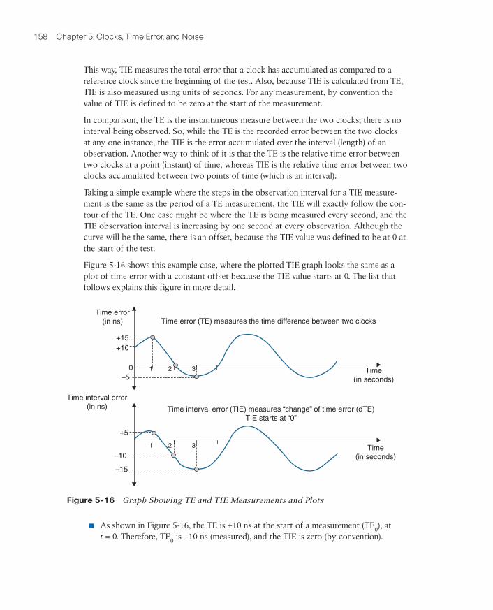
158 Chapter 5: Clocks, Time Error, and Noise
This way, TIE measures the total error that a clock has accumulated as compared to a reference clock since the beginning of the test. Also, because TIE is calculated from TE, TIE is also measured using units of seconds. For any measurement, by convention the value of TIE is defined to be zero at the start of the measurement.
In comparison, the TE is the instantaneous measure between the two clocks; there is no interval being observed. So, while the TE is the recorded error between the two clocks at any one instance, the TIE is the error accumulated over the interval (length) of an observation. Another way to think of it is that the TE is the relative time error between two clocks at a point (instant) of time, whereas TIE is the relative time error between two clocks accumulated between two points of time (which is an interval).
Taking a simple example where the steps in the observation interval for a TIE measure-ment is the same as the period of a TE measurement, the TIE will exactly follow the con-tour of the TE. One case might be where the TE is being measured every second, and the TIE observation interval is increasing by one second at every observation. Although the curve will be the same, there is an offset, because the TIE value was defined to be at 0 at the start of the test.
Figure 5-16 shows this example case, where the plotted TIE graph looks the same as a plot of time error with a constant offset because the TIE value starts at 0. The list that follows explains this figure in more detail.
Time error (TE) measures the time difference between two clocks
Time interval error (TIE) measures “change” of time error (dTE)TIE starts at “0”
Time error(in ns)
Time(in seconds)
+15
+5
+10
–10
–15
0–5
1 2 3
1 2 3 Time(in seconds)
Time interval error(in ns)
Figure 5-16 Graph Showing TE and TIE Measurements and Plots
■ As shown in Figure 5-16, the TE is +10 ns at the start of a measurement (TE0), at t = 0. Therefore, TE0 is +10 ns (measured), and the TIE is zero (by convention).
9780136836254_print.indb 158 29/04/21 6:57 pm
Time Error 159
■ Assume that the observation interval is 1 second. After the first observation interval, from Figure 5-16, TE1 is 15 ns. The TIE calculated for this interval will be (TE1 - TE0) = 5 ns.
■ After the second observation interval, assume TE2 is 0 ns. The TIE calculated now will be (TE2 - TE0) = -10 ns. Note that this calculation is for the second observation interval and the interval for calculations really became 2 seconds.
■ The observation interval keeps increasing until the end of the entire measurement test.
There are other clock metrics (discussed later in this chapter), such as MTIE and TDEV, that are calculated and derived from the TIE measurements. TIE, which is primarily a measurement of phase accuracy, is the fundamental measurement of the clock metrics.
Some conclusions that you can draw based on plotted TIE on a graph are as follows:
■ An ever-increasing trend in the TIE graph suggests that the measured clock has a frequency offset (compared to the reference clock). You can infer this because the frequency offset will be seen in each time error value and hence will get reflected in TIE calculations.
■ If TIE graph shows a large value at the start of the measurement interval and starts converging slowly toward zero, it might suggest that the clock or PLL is not yet locked to the reference clock or is slow in locking or responding to the reference input.
Note that the measurement of the change in TE at each interval really becomes measure-ment of a short-term variation, or jitter, in the clock signals, or what is sometimes called timing jitter. And as TIE is a measurement of the change in phase, it becomes a perfect measurement for capturing jitter.
Now it is time to revisit the concepts of accuracy and stability from Chapter 1, “Introduction to Synchronization and Timing.” These are two terms that have a very precise meaning in the context of timing.
For synchronization, accuracy measures how close one clock is to the reference clock. And this measurement is related to the maximum absolute TE (or max|TE|). So, a clock that closely follows the reference clock with a very small offset is an accurate clock.
On the other hand, stability refers to the change and the speed of change in the clock during a given observation interval, while saying nothing about how close it is to a reference clock.
As shown in Figure 5-17, an accurate clock might not be a very stable clock, or a very stable clock might not be accurate, and so on. As the end goal is to have the most stable as well as the most accurate clock possible, a clock is measured on both aspects. The metrics that quantify both these aspects become the timing characteristics of a clock.
9780136836254_print.indb 159 29/04/21 6:57 pm
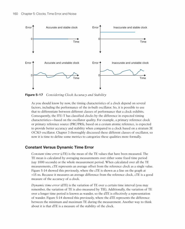
160 Chapter 5: Clocks, Time Error, and Noise
Accurate and stable clockError
Error
0 0
00
Time
Error Inaccurate and stable clock
Inaccurate and unstable clock
Time
Time
ErrorAccurate and unstable clock
Time
Figure 5-17 Considering Clock Accuracy and Stability
As you should know by now, the timing characteristics of a clock depend on several factors, including the performance of the in-built oscillator. So, it is possible to use that to differentiate between different classes of performance that a clock exhibits. Consequently, the ITU-T has classified clocks by the difference in expected timing characteristics—based on the oscillator quality. For example, a primary reference clock or primary reference source (PRC/PRS), based on a cesium atomic reference, is expected to provide better accuracy and stability when compared to a clock based on a stratum 3E OCXO oscillator. Chapter 3 thoroughly discussed these different classes of oscillator, so now it is time to define some metrics to categorize these qualities more formally.
Constant Versus Dynamic Time Error
Constant time error (cTE) is the mean of the TE values that have been measured. The TE mean is calculated by averaging measurements over either some fixed time period (say 1000 seconds) or the whole measurement period. When calculated over all the TE measurements, cTE represents an average offset from the reference clock as a single value. Figure 5-14 showed this previously, where the cTE is shown as a line on the graph at +15 ns. Because it measures an average difference from the reference clock, cTE is a good measure of the accuracy of a clock.
Dynamic time error (dTE) is the variation of TE over a certain time interval (you may remember, the variation of TE is also measured by TIE). Additionally, the variation of TE over a longer time period is known as wander, so the dTE is effectively a representation of wander. Figure 5-14 showed this previously, where the dTE represents the difference between the minimum and maximum TE during the measurement. Another way to think about it is that dTE is a measure of the stability of the clock.
M05_Hagarty_CH05_p139-178.indd 160 30/04/21 6:20 pm
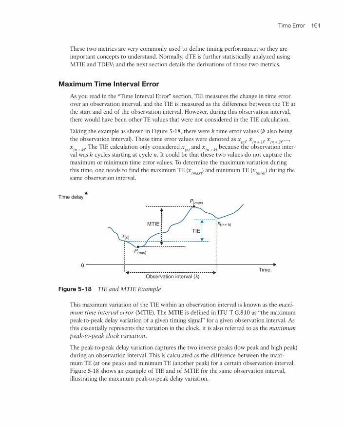
Time Error 161
These two metrics are very commonly used to define timing performance, so they are important concepts to understand. Normally, dTE is further statistically analyzed using MTIE and TDEV; and the next section details the derivations of those two metrics.
Maximum Time Interval Error
As you read in the “Time Interval Error” section, TIE measures the change in time error over an observation interval, and the TIE is measured as the difference between the TE at the start and end of the observation interval. However, during this observation interval, there would have been other TE values that were not considered in the TIE calculation.
Taking the example as shown in Figure 5-18, there were k time error values (k also being the observation interval). These time error values were denoted as x(n), x(n + 1), x(n + 2),…, x(n + k). The TIE calculation only considered x(n) and x(n + k) because the observation inter-val was k cycles starting at cycle n. It could be that these two values do not capture the maximum or minimum time error values. To determine the maximum variation during this time, one needs to find the maximum TE (x(max)) and minimum TE (x(min)) during the same observation interval.
x(n + k)
x(n)
P(max)
P(min)
Time delay
Time0
MTIE
Observation interval (k)
TIE
Figure 5-18 TIE and MTIE Example
This maximum variation of the TIE within an observation interval is known as the maxi-mum time interval error (MTIE). The MTIE is defined in ITU-T G.810 as “the maximum peak-to-peak delay variation of a given timing signal” for a given observation interval. As this essentially represents the variation in the clock, it is also referred to as the maximum peak-to-peak clock variation.
The peak-to-peak delay variation captures the two inverse peaks (low peak and high peak) during an observation interval. This is calculated as the difference between the maxi-mum TE (at one peak) and minimum TE (another peak) for a certain observation interval. Figure 5-18 shows an example of TIE and of MTIE for the same observation interval, illustrating the maximum peak-to-peak delay variation.
9780136836254_print.indb 161 29/04/21 6:57 pm
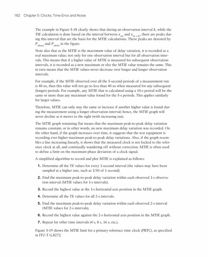
162 Chapter 5: Clocks, Time Error, and Noise
The example in Figure 5-18 clearly shows that during an observation interval k, while the TIE calculation is done based on the interval between x(n) and x(n + k), there are peaks dur-ing this interval that are the basis for the MTIE calculations. These peaks are denoted by P(max) and P(min) in the figure.
Note also that as the MTIE is the maximum value of delay variation, it is recorded as a real maximum value; not only for one observation interval but for all observation inter-vals. This means that if a higher value of MTIE is measured for subsequent observation intervals, it is recorded as a new maximum or else the MTIE value remains the same. This in turn means that the MTIE values never decrease over longer and longer observation intervals.
For example, if the MTIE observed over all the 5-second periods of a measurement run is 40 ns, then this value will not go to less than 40 ns when measured for any subsequent (longer) periods. For example, any MTIE that is calculated using a 10-s period will be the same or more than any maximum value found for the 5-s periods. This applies similarly for larger values.
Therefore, MTIE can only stay the same or increase if another higher value is found dur-ing the measurement using a longer observation interval; hence, the MTIE graph will never decline as it moves to the right (with increasing tau).
The MTIE graph remaining flat means that the maximum peak-to-peak delay variation remains constant; or in other words, no new maximum delay variation was recorded. On the other hand, if the graph increases over time, it suggests that the test equipment is recording ever-higher maximum peak-to-peak delay variations. Also, if the graph resem-bles a line increasing linearly, it shows that the measured clock is not locked to the refer-ence clock at all, and continually wandering off without correction. MTIE is often used to define a limit on the maximum phase deviation of a clock signal.
A simplified algorithm to record and plot MTIE is explained as follows:
1. Determine all the TE values for every 1-second interval (the values may have been sampled at a higher rate, such as 1/30 of 1 second).
2. Find the maximum peak-to-peak delay variation within each observed 1-s observa-tion interval (MTIE values for 1-s intervals).
3. Record the highest value at the 1-s horizontal axis position in the MTIE graph.
4. Determine all the TE values for all 2-s intervals.
5. Find the maximum peak-to-peak delay variation within each observed 2-s interval (MTIE values for 2-s intervals).
6. Record the highest value against the 2-s horizontal axis position in the MTIE graph.
7. Repeat for other time intervals (4 s, 8 s, 16 s, etc.).
Figure 5-19 shows the MTIE limit for a primary reference time clock (PRTC), as specified in ITU-T G.8272.
9780136836254_print.indb 162 29/04/21 6:57 pm
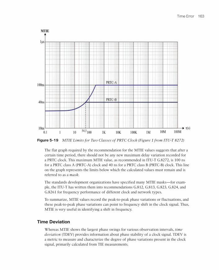
Time Error 163
Figure 5-19 MTIE Limits for Two Classes of PRTC Clock (Figure 1 from ITU-T 8272)
The flat graph required by the recommendation for the MTIE values suggests that after a certain time period, there should not be any new maximum delay variation recorded for a PRTC clock. This maximum MTIE value, as recommended in ITU-T G.8272, is 100 ns for a PRTC class A (PRTC-A) clock and 40 ns for a PRTC class B (PRTC-B) clock. This line on the graph represents the limits below which the calculated values must remain and is referred to as a mask.
The standards development organizations have specified many MTIE masks—for exam-ple, the ITU-T has written them into recommendations G.812, G.813, G.823, G.824, and G.8261 for frequency performance of different clock and network types.
To summarize, MTIE values record the peak-to-peak phase variations or fluctuations, and these peak-to-peak phase variations can point to frequency shift in the clock signal. Thus, MTIE is very useful in identifying a shift in frequency.
Time Deviation
Whereas MTIE shows the largest phase swings for various observation intervals, time deviation (TDEV) provides information about phase stability of a clock signal. TDEV is a metric to measure and characterize the degree of phase variations present in the clock signal, primarily calculated from TIE measurements.
9780136836254_print.indb 163 29/04/21 6:57 pm
164 Chapter 5: Clocks, Time Error, and Noise
Unlike MTIE, which records the difference between the high and low peaks of phase variations, TDEV primarily focuses on how frequent and how stable (or unstable) such phase variations are occurring over a given time—note the importance of “over a given time.” This is important because both “how frequent” and “how stable” parameters would change by changing the time duration of the measurements. For example, a significant error occurring every second of a test can be considered a frequently occurring error. But if that was the only error that occurred for the next hour, the error cannot be considered to be a frequently occurring error.
Consider a mathematical equation that divides the total phase variations (TE values) by the total test time; you will realize that if there are less phase variations over a long time, this equation produces a low value. However, the result from the equation increases if there are more phase variations during the same test time. This sort of equation is used for TDEV calculations to determine the quality of the clock.
The low frequency phase variations could appear to be occurring randomly. Only if such events are occurring less often over a longer time can these be marked as outliers. And this results in gaining confidence in the long-term quality of the clock. Think of toss-ing five coins simultaneously, and with the first toss, all five coins come down heads! Without tossing those coins a lot more times, you cannot be sure if that was an outlier (a random event) or if something strange is wrong with the coins.
The TDEV of a clock defines the limit of any randomness (or outliers) in the behavior of a clock. The degree of this randomness is a measure of the low frequency phase variation (wander), which can be statistically calculated from TIE measurements and plotted on graphs, using a TDEV calculation.
According to ITU-T G.810, TDEV is defined as “a measure of the expected time variation of a signal as a function of integration time.” So, TDEV is particularly useful in reveal-ing the presence of several noise processes in clocks over a given time interval; and this calculated measurement is compared to the limit (specified as a mask in the recommenda-tions) for each clock type.
Usually, instability of a system is expressed in terms of some statistical representation of its performance. Mathematically, variance or standard deviation are usual metrics that would provide an adequate view to express such instability. However, for clocks, it has been shown that the usual variance or standard deviation calculation has a problem—the calculation does not converge.
The idea of convergence can be explained with a generic example. A dataset composed of a large collection of values with a Gaussian distribution will have a specific mean and variance. The mean shows the average value, and the variance shows how closely the values cluster around the mean—much like the stability of a clock. Now, if one were to calculate these values using a small subset or sample of these values, then the level of confidence in those metrics would be low—much like the toss of five coins. And as these parameters are calculated using larger and larger samples of this example dataset, the confidence in these metrics increases. The increase in confidence here means that variance moves toward a true value for the given dataset—this is referred to as conver-gence of variance. However, for clocks and oscillators, no matter how large the sample
9780136836254_print.indb 164 29/04/21 6:57 pm
Time Error 165
of variations is, apparently there is no evidence of this variance value converging. To deal with this deficiency, one of the alternative approaches is to use TDEV.
Rather than understanding the exact formula for calculating TDEV, it might be better to see the TDEV measure as a root mean square (RMS) type of metric to capture clock noise. Mathematically, RMS is calculated by first taking a mean (average) of square values of the sample data and then taking a square root of it. The key aspect of this calculation is that it averages out extremes or outliers in the sample (much more than the normal mean). Interestingly, the extremes average out more and more as the sample data increases.
Thus, TDEV becomes a highly averaged value. And if the noise in the clock is occurring rarely, the degree (or magnitude) of this rarely occurring error starts diminishing over lon-ger periods of measurement. An example might be something occurring rarely or seldom, such as errors introduced by environmental changes over the course of the day (diurnal rhythms), such as the afternoon sun striking the exterior metal panel of the clock.
So, to gain confidence in the TDEV values (primarily to discard the rare noise occur-rence in clock), the tests are usually quite long, at least several times longer than the usual MTIE observation intervals. For example, ITU-T G.811 calls for running TDEV tests for 12 times the maximum observation interval.
Compared to TDEV, you might notice that MTIE is perfectly suited to catch outliers in samples of TIE measurements. MTIE is a detector of peaks, but TDEV is a measure of wander over varying observation time intervals and is well suited to characterization of wander noise. It can do that because it is very good at averaging out short-term and rare variations.
So, it makes sense that TDEV is used alongside MTIE as metrics to characterize the quality of clock. As is the case for MTIE, ITU-T recommendations also specify TDEV masks for the same purpose. These masks show the maximum permissible values for both TDEV and MTIE for different clock types and in different conditions.
Noise
In the timing world, noise is an unwanted disturbance in a clock signal—the signal is still there, and it is good, but it is not as perfect as one would like. Noise arises over both the short term, say for a single sampling period, as well as over much longer timeframes—up to the lifetime of the clock. Because there are several factors that can introduce noise, the amount and type of noise can vary greatly between different systems.
The metrics that are discussed in this chapter try to quantify the noise that a clock can generate at its output. For example, max|TE| represents the maximum amount of noise that can be generated by a clock. Similarly, cTE and dTE also characterize different aspects of the noise of a clock.
Noise is classified as either jitter or wander. As seen in the preceding section “Jitter and Wander,” by convention, jitter is the short-term variation, and wander is the long-term variation of the measured clock compared to the reference clock. The ITU-T G.810 standard defines jitter as phase variation with a rate of change greater than or equal
9780136836254_print.indb 165 29/04/21 6:57 pm
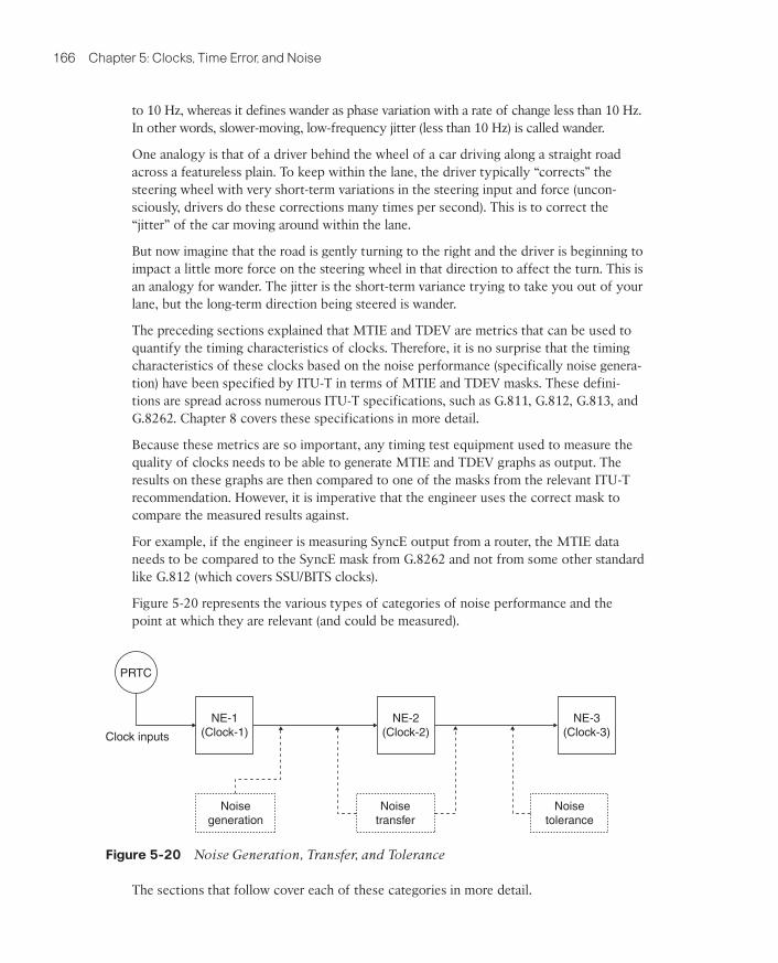
166 Chapter 5: Clocks, Time Error, and Noise
to 10 Hz, whereas it defines wander as phase variation with a rate of change less than 10 Hz. In other words, slower-moving, low-frequency jitter (less than 10 Hz) is called wander.
One analogy is that of a driver behind the wheel of a car driving along a straight road across a featureless plain. To keep within the lane, the driver typically “corrects” the steering wheel with very short-term variations in the steering input and force (uncon-sciously, drivers do these corrections many times per second). This is to correct the “jitter” of the car moving around within the lane.
But now imagine that the road is gently turning to the right and the driver is beginning to impact a little more force on the steering wheel in that direction to affect the turn. This is an analogy for wander. The jitter is the short-term variance trying to take you out of your lane, but the long-term direction being steered is wander.
The preceding sections explained that MTIE and TDEV are metrics that can be used to quantify the timing characteristics of clocks. Therefore, it is no surprise that the timing characteristics of these clocks based on the noise performance (specifically noise genera-tion) have been specified by ITU-T in terms of MTIE and TDEV masks. These defini-tions are spread across numerous ITU-T specifications, such as G.811, G.812, G.813, and G.8262. Chapter 8 covers these specifications in more detail.
Because these metrics are so important, any timing test equipment used to measure the quality of clocks needs to be able to generate MTIE and TDEV graphs as output. The results on these graphs are then compared to one of the masks from the relevant ITU-T recommendation. However, it is imperative that the engineer uses the correct mask to compare the measured results against.
For example, if the engineer is measuring SyncE output from a router, the MTIE data needs to be compared to the SyncE mask from G.8262 and not from some other standard like G.812 (which covers SSU/BITS clocks).
Figure 5-20 represents the various types of categories of noise performance and the point at which they are relevant (and could be measured).
PRTC
Clock inputs
NE-1(Clock-1)
Noisegeneration
Noisetransfer
Noisetolerance
NE-2(Clock-2)
NE-3(Clock-3)
Figure 5-20 Noise Generation, Transfer, and Tolerance
The sections that follow cover each of these categories in more detail.
9780136836254_print.indb 166 29/04/21 6:57 pm
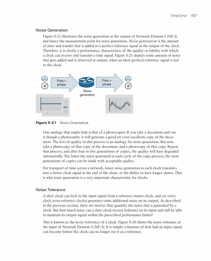
Time Error 167
Noise Generation
Figure 5-21 illustrates the noise generation at the output of Network Element-1 (NE-1) and hence the measurement point for noise generation. Noise generation is the amount of jitter and wander that is added to a perfect reference signal at the output of the clock. Therefore, it is clearly a performance characteristic of the quality or fidelity with which a clock can receive and transmit a time signal. Figure 5-21 depicts some amount of noise that gets added and is observed at output, when an ideal (perfect) reference signal is fed to the clock.
Freq +phase
Freq +phase
Noisegeneration
Figure 5-21 Noise Generation
One analogy that might help is that of a photocopier. If you take a document and run it though a photocopier, it will generate a good (or even excellent) copy of the docu-ment. The loss of quality in that process is an analogy for noise generation. But now, take a photocopy of that copy of the document, and a photocopy of that copy. Repeat that process, and after four to five generations of copies, the quality will have degraded substantially. The lower the noise generated in each cycle of the copy process, the more generations of copies can be made with acceptable quality.
For transport of time across a network, lower noise generation in each clock translates into a better clock signal at the end of the chain, or the ability to have longer chains. That is why noise generation is a very important characteristic for clocks.
Noise Tolerance
A slave clock can lock to the input signal from a reference master clock, and yet every clock (even reference clocks) generates some additional noise on its output. As described in the previous section, there are metrics that quantify the noise that is generated by a clock. But how much noise can a slave clock receive (tolerate) on its input and still be able to maintain its output signal within the prescribed performance limits?
This is known as the noise tolerance of a clock. Figure 5-20 shows the noise tolerance at the input of Network Element-3 (NE-3). It is simply a measure of how bad an input signal can become before the clock can no longer use it as a reference.
9780136836254_print.indb 167 29/04/21 6:57 pm
168 Chapter 5: Clocks, Time Error, and Noise
Going back to the photocopier analogy, the noise tolerance is the limit at which the pho-tocopier can only just read the input document well enough to produce a readable copy. Any further degradation and it cannot produce a satisfactory output.
Like noise generation, noise tolerance is also specified as MTIE and TDEV masks for each class of clock performance. Up until the maximum permissible values of noise specified in ITU-T recommendations is applied at the input of a clock, the output of the clock should continue to operate within the expected performance limits. These masks are specified in the same ITU-T specifications that cover noise generation, such as G.812, G.813, G.823, G.824, and G.8262.
What happens when the noise at the input of a clock exceeds the permissible limits—what should be the action of a clock? The clock could do one or more of the following:
■ Report an alarm, warning that it has lost the lock to the input clock
■ Switch to another reference clock if there are backup references available
■ Go into holdover (operating without an external reference input) and raise an alarm warning of the change of status and quality
Noise Transfer
To synchronize network elements to a common timing source, there can be at least two different approaches—external clock distribution and line timing clock distribution.
An external clock distribution or frequency distribution network (refer to the sec-tion “Legacy Synchronization Networks” in Chapter 2, “Usage of Synchronization and Timing”) becomes challenging because the network elements are normally geographically dispersed. So, building a dedicated synchronization network to each node could become very costly, and hence this method is often not preferred.
The other approach is to cascade the network elements and use the line clocking (again refer to the section “Legacy Synchronization Networks” in Chapter 2), where the clock is passed from one network element to the next element, as in a daisy chain. Figure 5-20 shows the clock distribution model using the line clocking approach, where NE-1 is pass-ing the clock to NE-2 and then subsequently to NE-3.
From the previous section on noise generation, you know that every clock will generate additional noise on the output of the clock compared to the input. When networks are designed as a daisy chain clock distribution, the noise generated at one clock is being passed as input to the next clock synchronized to it. This way, noise not only cascades down to all the clocks below it in the chain, but the noise gets amplified during transfer. To try to lessen that, the accumulated noise needs to be somehow reduced or filtered at the output of the clock (on each network element).
This propagation of noise from input to output of a node is called noise transfer and can be defined as the noise that is seen at the output of the clock due to the noise that is fed to the input of the clock. The filtering capabilities of the clock determines the amount
9780136836254_print.indb 168 29/04/21 6:57 pm
Holdover Performance 169
of noise being transferred through a clock from the input to the output. Obviously, less noise transfer is desirable. Figure 5-20 shows the noise that NE-2 transferred to NE-3 based on noise it was subjected to from NE-1.
Again, as with the ITU-T clock specifications for noise generation and tolerance, MTIE and TDEV masks are used to specify the allowed amount of noise transfer. Remember that each clock node has a PLL with filtering capabilities (LPF and HPF) that can fil-ter out noise based on the clock bandwidth (refer to the earlier section “Low-Pass and High-Pass Filters”).
The main metric used to describe how noise is passed from input to output is clock bandwidth, which was explained in the section “Low-Pass and High-Pass Filters.” For example, the noise transfer of an Option 1 EEC is described in clause 10.1 of ITU-T G.8262 as follows: “The minimum bandwidth requirement for an EEC is 1 Hz. The maximum bandwidth requirement for an EEC is 10 Hz.”
Holdover PerformanceGiven an accurate reference clock as an input signal, one can achieve a well-synchronized clock. This is the fundamental principle of timing synchronization whereby a master clock drives the slave clock, always assuming that the master clock itself is stable and accurate.
Occasionally, there will be cases where the master clock becomes unavailable. During such periods, the local clock is no longer disciplined by a master (or reference) clock. Most synchronization-based applications need to know the amount of frequency drift that can occur during such events.
The time during which a clock does not have a reference clock to synchronize to is called clock holdover. In this state, the clock behaves like a flywheel that keeps spinning at a constant speed even when it is not being actively driven, so this is sometimes also referred to as flywheel mode. And the measure of the speed with which a slave clock drifts away from the reference or master clock is called its holdover performance. The clock’s ability to maintain the same frequency over an interval of time without a refer-ence frequency being available is called frequency holdover. Similarly, time or phase holdover is the ability to maintain phase accuracy over an interval of time without the external phase reference.
This synchronization across network elements is achieved either via a physical signal (such as SyncE) or via precision time protocol (PTP) packets carrying timing synchroniza-tion information. There is even the ability to combine both approaches in a hybrid clock-ing architecture, whereby frequency is carried with SyncE and phase synchronization with PTP packets. Chapter 7, “Precision Time Protocol,” delves into this a little more.
A physical link failure (or fault) will break the frequency distribution via SyncE or inter-rupt the PTP packet path between slave and master. During such events, the slave clock will start slowly “drifting” away from the reference or master clock. This frequency and phase drift, besides depending on many external factors, also depends on components used for the local clock and the characteristics of the PLL circuitry.
9780136836254_print.indb 169 29/04/21 6:57 pm
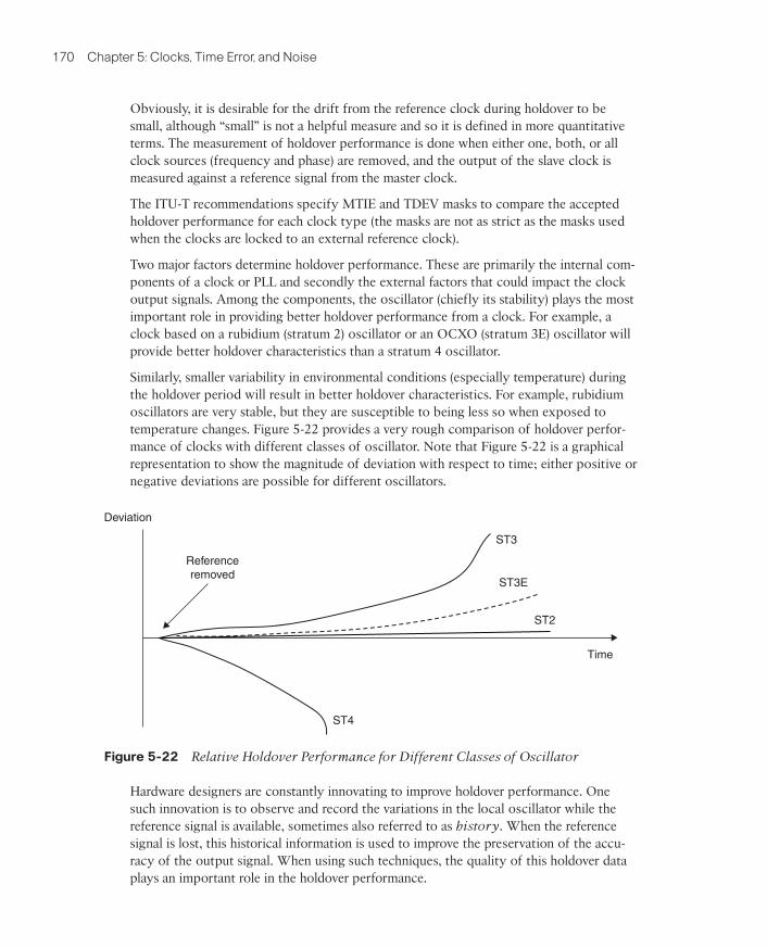
170 Chapter 5: Clocks, Time Error, and Noise
Obviously, it is desirable for the drift from the reference clock during holdover to be small, although “small” is not a helpful measure and so it is defined in more quantitative terms. The measurement of holdover performance is done when either one, both, or all clock sources (frequency and phase) are removed, and the output of the slave clock is measured against a reference signal from the master clock.
The ITU-T recommendations specify MTIE and TDEV masks to compare the accepted holdover performance for each clock type (the masks are not as strict as the masks used when the clocks are locked to an external reference clock).
Two major factors determine holdover performance. These are primarily the internal com-ponents of a clock or PLL and secondly the external factors that could impact the clock output signals. Among the components, the oscillator (chiefly its stability) plays the most important role in providing better holdover performance from a clock. For example, a clock based on a rubidium (stratum 2) oscillator or an OCXO (stratum 3E) oscillator will provide better holdover characteristics than a stratum 4 oscillator.
Similarly, smaller variability in environmental conditions (especially temperature) during the holdover period will result in better holdover characteristics. For example, rubidium oscillators are very stable, but they are susceptible to being less so when exposed to temperature changes. Figure 5-22 provides a very rough comparison of holdover perfor-mance of clocks with different classes of oscillator. Note that Figure 5-22 is a graphical representation to show the magnitude of deviation with respect to time; either positive or negative deviations are possible for different oscillators.
ST3
ST3E
ST2
ST4
Referenceremoved
Deviation
Time
Figure 5-22 Relative Holdover Performance for Different Classes of Oscillator
Hardware designers are constantly innovating to improve holdover performance. One such innovation is to observe and record the variations in the local oscillator while the reference signal is available, sometimes also referred to as history. When the reference signal is lost, this historical information is used to improve the preservation of the accu-racy of the output signal. When using such techniques, the quality of this holdover data plays an important role in the holdover performance.
9780136836254_print.indb 170 29/04/21 6:57 pm
Holdover Performance 171
There are cases where multiple paths of synchronization are available, and not all are lost simultaneously. For the hybrid synchronization case, where frequency synchronization is achieved via physical network (SyncE) and phase synchronization is achieved via PTP packets, it may be that only one of the synchronization transport paths breaks (such as, only the PTP packet path or just the frequency synchronization path). For such cases, one of the synchronization modes could move into holdover.
For example, it could be that the PTP path to the master is lost (for example, due to logi-cal path failure to the PTP master) but frequency synchronization (SyncE) is still available. In this case, the frequency stays locked to the reference and just the phase/time moves into holdover.
Why is holdover performance important, and how long should good holdover perfor-mance be required?
As an example, let us examine the case of a 4G LTE-Advanced cell site, which may have a phase alignment requirement to be always within ±1.5 µs of its master. This cell site is equipped with a GPS receiver and external antenna to synchronize its clock to this level of phase accuracy. Suppose this GPS antenna fails for some reason (say, a lightning strike). In that case, the clock in this cell site equipment will immediately move into holdover. The operation of this cell site can only continue so long as its clock phase alignment of that cell site radio stays within ±1.5 µs of accuracy.
Should this GPS antenna failure happen during the night, it might take some time for operations staff to discover and locate the failure, and then dispatch a technician to the correct location. If it was a long weekend, it might take quite some time for the techni-cian to reach the location and fix the issue (assuming the technician knows what the problem is and has spares for the GPS antenna readily available).
Of course, it would be very convenient if, during this whole duration, the clock was able to stay within a phase alignment of ±1.5 µs and provide uninterrupted service to that area. If the maximum time to detect and correct this fault is (say) 24 hours, then for unin-terrupted service, the clock on this cell site requires a holdover period of 24 hours for ±1.5 µs. In fact, the generally accepted use case at the ITU-T is that a clock should need holdover performance for up to 72 hours (considering a long weekend).
Note that this requirement (24 hours for ±1.5 µs) is quite a strict holdover specification and just about all currently deployed systems (cell site radios and routers) are not able to achieve this level of holdover. Being able to do it for 72 hours is very difficult and requires a clock with a very high-quality oscillator, such as one based on rubidium.
Adding to the difficulty, the weather conditions at a cell site (up some mountaintop) might be extremely challenging with only minimal control of environmental conditions for the equipment. Temperature is a very significant factor contributing to the stability of an oscillator, and that stability feeds directly into holdover performance. For this reason, the ITU-T G.8273.2 specification for a PTP boundary and slave clock defines the required holdover performance in absence of PTP packets for both cases—constant temperature and variable temperature.
9780136836254_print.indb 171 29/04/21 6:57 pm
172 Chapter 5: Clocks, Time Error, and Noise
Transient ResponseHoldover is the state that a clock transitions to whenever the input reference clock is lost. It has been shown that providing good, long-duration holdover to a failure of the refer-ence signal is neither easy nor inexpensive. However, there could be multiple reference clocks simultaneously available to a slave clock, offering the ability to provide backup signals in the case of failure. Consequently, network designers prefer a design where mul-tiple references are available to the network elements—providing redundancy and backup for timing synchronization.
The question arises, how should the clock behave when an input reference clock is lost and the clock decides to select the second-best clock source as the input reference? The behavior during this event is characterized as the transient response of a clock.
Multiple reference inputs to a clock could be traceable (via different paths) to the same source of time (such as a PRTC) or back to different sources. The clock quality informa-tion (such as Ethernet synchronization messaging channel (ESMC) and PTP packets) sent through the network shows the quality of the source of time that these separate refer-ences offer. The software managing the slave clocks then decides which backup reference clock to use based on the quality information. As expected, a high-quality reference is preferred over a lower-quality reference clock.
For cases where there are multiple inputs, the network designer might assign the input references a priority, so that the slave clock can decide in what order the input is pre-ferred. So, when the highest priority (say priority 1) reference clock fails, the slave must decide whether there is another reference available to provide an input signal. The slave selects one of the remaining sources available out of those signaling the highest quality level. If more than one source signal is available at that quality level, the slave selects the available reference with the highest priority (say, priority 2). The slave will then start to acquire this new input signal and continue to provide an output signal but now aligned to the new reference.
This switchover, referred to as reference clock change, is known as a transient event and the change in timing characteristics of a clock during such an event is referred to as tran-sient response. This is a very different event from a clock moving into the holdover state, because the change in reference clock happens very quickly, resulting in the slave clock being in the holdover state for only a very brief time.
These transients are thus divided in the ITU-T recommendations into two categories: long-term transients and short-term transients. Switching between two reference inputs is an example of a short-term transient. Long-term transient is another name for holdover.
Transient response specifies the noise that a slave clock generates during such events. Slave clocks are unlikely to be transparent during such events and could either transfer or gener-ate additional noise, which is measured as the transient response. Again, for each clock type, there are MTIE and TDEV masks in the ITU-T standards to specify the accepted transient response. For example, you can find MTIE and TDEV masks for transient response for clocks supporting SDH (E1) and SONET (T1) in clause 11 of ITU-T G.812.
9780136836254_print.indb 172 29/04/21 6:57 pm
Measuring Time Error 173
Measuring Time ErrorThis chapter explores several definitions and limits of time error, and numerous metrics to quantify it, as well as examining the impact of time error on applications. In summary, time error, essentially the difference between a slave clock and a reference or master clock, is primarily measured using four metrics: cTE, dTE, max|TE|, and TIE. From those basic measurements, engineers have statistically derived MTIE and TDEV from TIE, in combination with the application of different filters.
ITU-T recommendations specify the allowed limits for these different metrics of time error. The metrics cTE and max|TE| are defined in terms of time (such as nanoseconds). dTE, being the change of the time error function over time, is characterized using TIE and is then compared to a mask expressed in MTIE and TDEV, which defines the permis-sible limits for that type of clock.
Some ITU-T recommendations define allowed limits for a single standalone clock (a single network element), and others specify clock performance at the final output of a timing chain in an end-to-end network. You should not mix these two types of specifica-tions, because limits that apply to the standalone case do not apply to the network case. Similarly, masks used to define the limits on a standalone clock do not apply to the net-work. This is especially the case when discussing the testing of timing performance, as in Chapter 12, “Operating and Verifying Timing Solutions.”
For each type and class of standalone clock, all four metrics, max|TE|, cTE, dTE, and TIE, are specified by these standards, while for the network case, max|TE| and dTE are specified. The cTE is not listed for network limits because the limits of max|TE| for the network case automatically include cTE, which might be added by any one clock in the chain of clocks.
The ITU-T specifies the various noise and/or time error constraints for almost all the clock types. For each one of the numerous clock specifications, the ITU-T recommenda-tions define all five aspects for timing characterization of a clock:
■ Noise generation
■ Noise tolerance
■ Noise transfer
■ Transient response
■ Holdover performance
Chapter 8 will cover these specifications in more detail.
Topology
As shown in Figure 5-23, the setup required for time error measurement testing includes
■ Timing testing equipment that can synthesize ideal reference clock signals.
■ Clock under test that would normally be embedded in a network element.
9780136836254_print.indb 173 29/04/21 6:57 pm
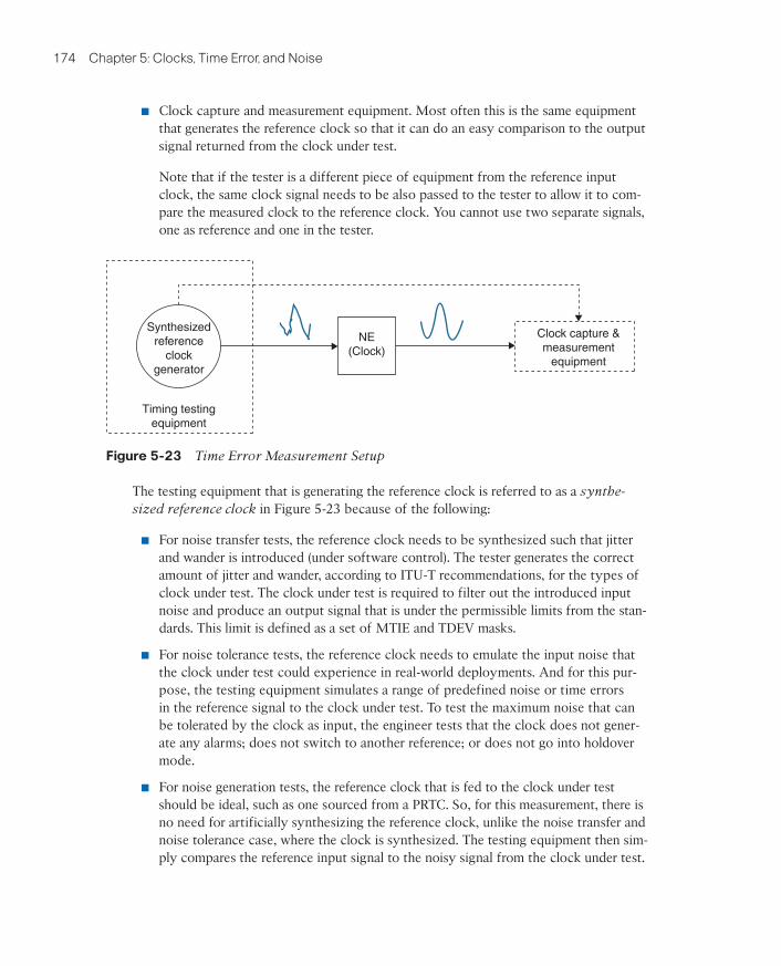
174 Chapter 5: Clocks, Time Error, and Noise
■ Clock capture and measurement equipment. Most often this is the same equipment that generates the reference clock so that it can do an easy comparison to the output signal returned from the clock under test.
Note that if the tester is a different piece of equipment from the reference input clock, the same clock signal needs to be also passed to the tester to allow it to com-pare the measured clock to the reference clock. You cannot use two separate signals, one as reference and one in the tester.
Synthesizedreference
clockgenerator
Timing testingequipment
NE(Clock)
Clock capture &measurement
equipment
Figure 5-23 Time Error Measurement Setup
The testing equipment that is generating the reference clock is referred to as a synthe-sized reference clock in Figure 5-23 because of the following:
■ For noise transfer tests, the reference clock needs to be synthesized such that jitter and wander is introduced (under software control). The tester generates the correct amount of jitter and wander, according to ITU-T recommendations, for the types of clock under test. The clock under test is required to filter out the introduced input noise and produce an output signal that is under the permissible limits from the stan-dards. This limit is defined as a set of MTIE and TDEV masks.
■ For noise tolerance tests, the reference clock needs to emulate the input noise that the clock under test could experience in real-world deployments. And for this pur-pose, the testing equipment simulates a range of predefined noise or time errors in the reference signal to the clock under test. To test the maximum noise that can be tolerated by the clock as input, the engineer tests that the clock does not gener-ate any alarms; does not switch to another reference; or does not go into holdover mode.
■ For noise generation tests, the reference clock that is fed to the clock under test should be ideal, such as one sourced from a PRTC. So, for this measurement, there is no need for artificially synthesizing the reference clock, unlike the noise transfer and noise tolerance case, where the clock is synthesized. The testing equipment then sim-ply compares the reference input signal to the noisy signal from the clock under test.
9780136836254_print.indb 174 29/04/21 6:57 pm
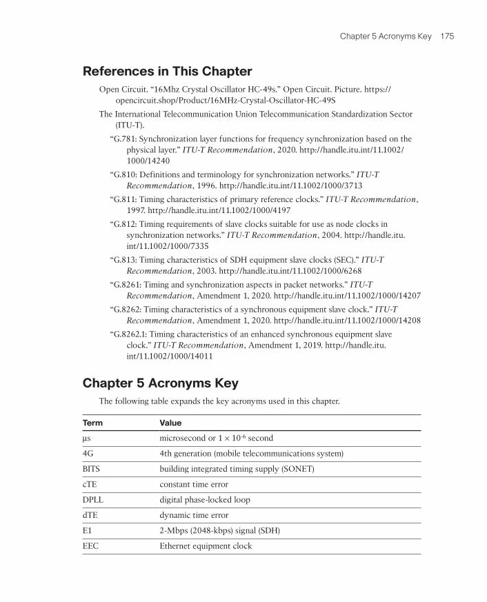
Chapter 5 Acronyms Key 175
References in This ChapterOpen Circuit. “16Mhz Crystal Oscillator HC-49s.” Open Circuit. Picture. https://
opencircuit.shop/Product/16MHz-Crystal-Oscillator-HC-49S
The International Telecommunication Union Telecommunication Standardization Sector (ITU-T).
“G.781: Synchronization layer functions for frequency synchronization based on the physical layer.” ITU-T Recommendation, 2020. http://handle.itu.int/11.1002/ 1000/14240
“G.810: Definitions and terminology for synchronization networks.” ITU-T Recommendation, 1996. http://handle.itu.int/11.1002/1000/3713
“G.811: Timing characteristics of primary reference clocks.” ITU-T Recommendation, 1997. http://handle.itu.int/11.1002/1000/4197
“G.812: Timing requirements of slave clocks suitable for use as node clocks in synchronization networks.” ITU-T Recommendation, 2004. http://handle.itu.int/11.1002/1000/7335
“G.813: Timing characteristics of SDH equipment slave clocks (SEC).” ITU-T Recommendation, 2003. http://handle.itu.int/11.1002/1000/6268
“G.8261: Timing and synchronization aspects in packet networks.” ITU-T Recommendation, Amendment 1, 2020. http://handle.itu.int/11.1002/1000/14207
“G.8262: Timing characteristics of a synchronous equipment slave clock.” ITU-T Recommendation, Amendment 1, 2020. http://handle.itu.int/11.1002/1000/14208
“G.8262.1: Timing characteristics of an enhanced synchronous equipment slave clock.” ITU-T Recommendation, Amendment 1, 2019. http://handle.itu.int/11.1002/1000/14011
Chapter 5 Acronyms KeyThe following table expands the key acronyms used in this chapter.
Term Value
µs microsecond or 1 × 10⁻⁶ second
4G 4th generation (mobile telecommunications system)
BITS building integrated timing supply (SONET)
cTE constant time error
DPLL digital phase-locked loop
dTE dynamic time error
E1 2-Mbps (2048-kbps) signal (SDH)
EEC Ethernet equipment clock
9780136836254_print.indb 175 29/04/21 6:57 pm
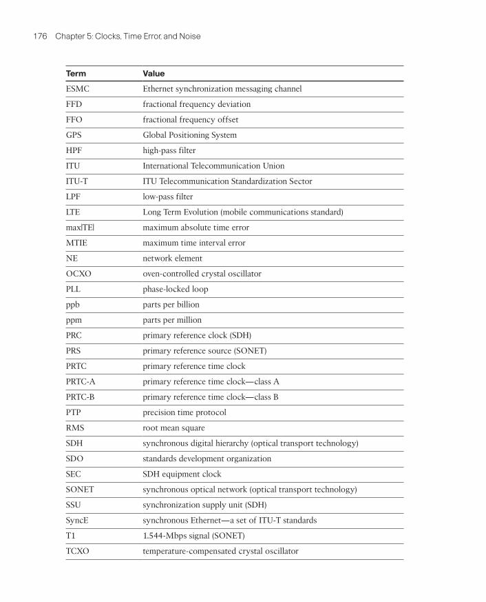
176 Chapter 5: Clocks, Time Error, and Noise
Term Value
ESMC Ethernet synchronization messaging channel
FFD fractional frequency deviation
FFO fractional frequency offset
GPS Global Positioning System
HPF high-pass filter
ITU International Telecommunication Union
ITU-T ITU Telecommunication Standardization Sector
LPF low-pass filter
LTE Long Term Evolution (mobile communications standard)
max|TE| maximum absolute time error
MTIE maximum time interval error
NE network element
OCXO oven-controlled crystal oscillator
PLL phase-locked loop
ppb parts per billion
ppm parts per million
PRC primary reference clock (SDH)
PRS primary reference source (SONET)
PRTC primary reference time clock
PRTC-A primary reference time clock—class A
PRTC-B primary reference time clock—class B
PTP precision time protocol
RMS root mean square
SDH synchronous digital hierarchy (optical transport technology)
SDO standards development organization
SEC SDH equipment clock
SONET synchronous optical network (optical transport technology)
SSU synchronization supply unit (SDH)
SyncE synchronous Ethernet—a set of ITU-T standards
T1 1.544-Mbps signal (SONET)
TCXO temperature-compensated crystal oscillator
9780136836254_print.indb 176 29/04/21 6:57 pm
Further Reading 177
Term Value
TDEV time deviation
TE time error
TIE time interval error
VCO voltage-controlled oscillator
VCXO voltage-controlled crystal oscillator
XO crystal oscillator
Further ReadingRefer to the following recommended sources for further information about the topics covered in this chapter.
ANSI: https://www.ansi.org
ETSI: https://www.etsi.org
ITU: https://www.itu.int
9780136836254_print.indb 177 29/04/21 6:57 pm
Index
Numbers1DM (One-way Delay Measurement),
29–301PSS, 80–81
phase inputs/outputs, 355–356time inputs/outputs, 355–356virtual PTP ports, 356–357
1xRTT handovers, 4762DM (Two-way Delay Measurement),
29, 302G networks, synchronization
requirements, 4542-MHz frequency, 773G networks, synchronization
requirements, 4543GPP (Third Generation Partnership
Project), 106–1095G networks
5G RAN, 488–4915GCN, 482–484absolute timing, 554–556architecture of, 478–480assisted partial timing, 548–550bandwidth, 481–482
CPRI, 487–488, 493–495deployment considerations, 520DRAN, 493–494eCPRI, 493–495eMBB, 478evolution of, 478–480frame structures, 481–482frequency deployments, 538frequency-only deployments, 535fronthaul timing, 550–551full on-path support, 541–543FWA, 478GNSS, 539–541holdovers, 531–532integrity verification, IEEE
1588-2019, 554–556ITU-T G.8265.1, 537ITU-T G.8271.1, 538–539ITU-T G.8271.2, 538–539ITU-T G.8275.1, 541–543ITU-T G.8275.2, 543–547, 548–550macro cells, 524–527MACsec, 556–559, 561–564midhaul timing, 550–551
9780136836254_print.indb 659 29/04/21 6:58 pm
660 5G networks
mMTC, 478MRTD, 508multi-profile with profile
interworking, 547–548networks
slicing, 496time error budget analysis,
501–505NR CRAN, 493–494NR synchronization requirements,
496–500phase deployments, 538phase network topologies, 538–539PTP security, 556–559RAN, 484–486, 488–491
centralized RAN, 552–553distributed RAN, 552–553functional splits, 491–492packetized RAN, 553–554
redundancy, 527–529GNSS, 529–530PTP, 530SyncE, 530
relative time budget analysis, 500–501
relative timing, 554–556RoE, 493–494scalable OFDM numerology,
481–482security, 556–559small cells, 524–527solution deployment options,
535–537spectrum, 480SyncE, 537, 541–543TaaS, 534–535TAE, 508
technology splits, 551–552third-party circuits, 532–534time deployments, 538topologies, 520–522transport architectures, 493–495uRLLC, 478use cases, 522–524vDU synchronization, 505–508
10-MHz frequency, 76–77
AaBMCA (alternate BMCA), 236absolute timing, 554–556AC (Attachment Circuits), TDM
networks, 31accuracy, time, 15acquiring state, clocks, 58ACR (Adaptive Clock Recovery), 32,
362–364acronyms keys
chapter 1, 16–17chapter 2, 35–37chapter 3, 92–95chapter 4, 132–137chapter 5, 175–177chapter 6, 209–211chapter 7, 283–287chapter 8, 342–345chapter 9, 437–442chapter 10, 512–516chapter 11, 567–571chapter 12, 653–657
active/passive probes, 641–643AES (Audio Engineering Society),
128AES67, 263, 269–270
9780136836254_print.indb 660 29/04/21 6:58 pm
CDMA2000, 2G/3G network synchronization requirements 661
aging, frequencies, 7aging oscillators, 56Announce messages, 214, 234–236ANSI, stratum levels of frequency
clocks, 59–61antennas
diversity, 463multi-antenna transmissions,
463–464assisted partial timing support,
PTP, 376–377assurance, networks, 629–630asymmetry
correction/calibration, 392–395dynamic asymmetry, 390–391PTP messages, 389
asymmetry correction, 226–228
delays, 225–226static asymmetry, 389–390
asynchronous networks, overview, 41–42
atomic clocks, 10, 11atomic oscillators, 55, 56–57audiovisual synchronization, 32–33augmentation systems, GNSS, 72–75automation, networks, 629–630aware/unaware nodes, PTP, 374–376
Bbackup timing, WAN, 33–34baluns, 77bandwidth
5G networks, 481–482packets, 361
BeiDou navigation satellite system, 70
BIPM (Bureau International des Poids et Mesures), 11, 12–13
BITS (Building Timing Integrated Supply), 77–78, 181–185
BMCA (Best Master Clock Algorithm), 236–237
BNC connectors, 350–351boundary clocks, 245–246BPF (Band-Pass Filters), 147–148bridges, defined, 112broadband
eMBB, 478mMTC, 478uRLLC, 478
BS (Base Stations)BS to BS synchronization, 462–463LTE-TDD wide area BS, 476UE to BS synchronization, 462
building clocks, 181bundle of ports, 195
CCA (Carrier Aggregation), 470–471cable
DOCSIS cable, non-mobile deployments, 431–432
phase synchronization, 26–28calibrating, timing, 596–598cascaded media converters, testing,
626–628CDMA, 449
1xRTT handovers, 4762G/3G network synchronization
requirements, 454CDMA2000, 2G/3G network
synchronization requirements, 454
9780136836254_print.indb 661 29/04/21 6:58 pm
662 CE (Carrier Ethernet), MEF Forum
CE (Carrier Ethernet), MEF Forum, 126–127
cell search, synchronization, 461cellular networks
evolution of, 444–448high band frequencies, 448low band frequencies, 446mid-band frequencies, 446
CEM (Circuit Emulation)TDM networks, 30–32timing solutions, 31–32
centralized RAN, 552–553cesium oscillators, 55–56Circular T, 11, 12–13cleanup, clock, 184clock offset, 47clockClass, 53clocks
acquiring state, 58ACR, 362–364attributes of, 54–55boundary clocks, 245–246BPF, 147–148building clocks, 181cleanup, 184clock signals, 139–140DCR, 364–365defined, 54delivery clocks, ITU-T phase/time
recommendations, 401–402dividers, 577ePRTC
ITU-T G.8272.1, 330–331timing, 330–331
FFD, 153–154free-running mode, 58, 185
frequency clocks, 62stratum levels, 59–61, 62–64testing in packet networks,
610–613time distribution hierarchies, 62
frequency errors, 153–154frequency synchronization, 577–579functions of, 140GM clocks, 65grandmaster (ordinary) clocks,
243–244ITU-T G.8266, 328–329ITU-T G.8273.1, 331timing, 328–329
hierarchy, 185–186holdovers
holdover mode, 59performance, 169–171specifications, 154state, 185
HPF, 147–148jitter, 146, 148–153locked mode, 58–59LPF, 146, 147measured clocks, 155modes, 57–59multipliers, 577MUX, 578node clocks, ITU-T G.812, 306noise, 148–149, 165–166, 199
generation, 167tolerance, 167–168transfers, 168–169transient events, 172transient response, 172
office clocks, 181
9780136836254_print.indb 662 29/04/21 6:58 pm
clocks 663
one-step clocks, 230–231oscillators, 140
aging, 56atomic oscillators, 55, 56–57cesium oscillators, 55–56crystal oscillators, 55, 56,
141–142hydrogen masers, 56OCXO, 55, 56, 142quartz oscillators, 55rubidium oscillators, 55, 56signal histories, 170TCXO, 55, 56, 142VCO, 143VCXO, 142
packet clocks, 64–65, 327–328performance, 326–327, 401–402
ITU-T, 305–308ITU-T G.8263, 327–328synchronization chains, 62–64T-BC testing, 629T-TSC testing, 629
phase-aware clocks, 579–581phase clocks
frameworks, 319–320ITU-T G.8273, 319–320
phase errors, 155PLL, 143–146, 152–153plot of phase deviations, 149–152PRC, 44–45, 600–603primary reference clocks
ITU-T G.811, 306ITU-T G.811.1, 306–307
PRTC, 64, 65, 403–404ITU-T G.8272.1, 330–331testing, 600–603timing, 329–331
PTP clocks, 242–243boundary clocks, 245–246domains, 220grandmaster (ordinary) clocks,
243–244overview, 218–219slave (ordinary) clocks,
244–245testing standalone PTP clocks,
613–629transparent clocks, 246–249
PTP-aware clocks, 581control plane processing,
584–586hardware-assisted
timestamping, 581–584packet processing, 584–586servo processing, 584–586
QL, 191–193, 354–355quality traceability, 51–53
clockClass, 53eESMC, 53ESMC, 53health bits, 53methods, 53SSM bits, 52, 53time of day messages, 53timing loops, 54
rearrangement, 201SEC, ITU-T G.813, 308selection algorithm. See traceabilityselection process, 199–201signal comparisons, 155signal noise. See noiseslave (ordinary) clocks, 244–245
ITU-T G.812, 306SEC, ITU-T G.813, 308
9780136836254_print.indb 663 29/04/21 6:58 pm
664 clocks
synchronous slave clocks, 314–315
telecom time slave clocks, 331–334
stratum 1 clocks, 61stratum 2 clocks, 61stratum 3E clocks, 61stratum 4 clocks, 61stratum 4E clocks, 61synchronous slave clocks
ITU-T G.8262, 314ITU-T G.8262.1, 314–315timing, 314–315
T-BC testing, 629TC, 65TDEV, 163–165TE, 154–156
cTE, 160, 385–386dTE, 160–161, 386–388max|TE|, 156–157, 385measuring, 173–174MTIE, 161–165. See also TIEnegative time error, 156positive time error, 156TIE, 157–160. See also MTIE
telecom boundary clocksITU-T G.8273.2, 331–332ITU-T G.8273.4, 333–334timing, 331–332
telecom grandmaster clocksITU-T G.8266, 328–329ITU-T G.8273.1, 331timing, 328–329, 331
telecom time slave clocksITU-T G.8273.2, 331–332ITU-T G.8273.4, 333–334timing, 331–334
telecom transparent clocksITU-T G.8273.3, 332–333timing, 332–333
T-GM clocks, 600–603time clocks
frameworks, 319–320ITU-T G.8273, 319–320
time-aware clocks, 579–581timing, packet clocks, 327–328traceability, 189–191transparent clocks, 246
end-to-end transparent clocks, 247–248, 249
peer-to-peer transparent clocks, 248–249
transparent clocks, 246–247T-TSC testing, 629two-step clocks, 230–231wander, 146, 148–153warm-up time, 57
CMDA radios, 24–25common network problems,
troubleshooting, 635–639CoMP (Coordinated Multipoint),
468–470, 475connectors
BNC connectors, 350–351DIN 1.0/2.3 connectors, 350, 352RJ-45 type connectors, 352–353SMB connectors, 350
consent, ITU-T, 294consumers of time synchronization, 88contributions, ITU-T, 293control plane processing, 584–586Coordinated Universal Time (UTC),
12–13correction field, PTP, 228
9780136836254_print.indb 664 29/04/21 6:58 pm
end-to-end networks 665
CPRI (Common Public Radio Interface), 121–122, 487–488, 493–495
crystal oscillators, 141–142OCXO, 55, 56TCXO, 55, 56
cTE (Constant Time Errors), 160, 385–386
CUPS (Control and User Plane Separation), 484
current datasets, 237
Ddata overflow, 22data underflow, 22datasets, 237–239DC (Dual Connectivity), 471–472DCR (Differential Clock Recovery),
32, 364–365default datasets, 237delays
1DM, 29–302DM, 29, 30packet networks, ITU-T G.8261.1,
312–313spread, 459variations, packets, 395–399
delegates, ITU-T, 293delivery clocks, ITU-T phase/time
recommendations, 401–402densification, 540digital interfaces (hierarchical), ITU-T
G.703, 309–310DIN 1.0/2.3 connectors, 350, 352distributed RAN, 493–494, 552–553diversity
antenna diversity, 463spatial diversity, 463
dividers, clocks, 577DOCSIS cable, non-mobile
deployments, 431–432DPLL (Digital Phase Locked Loops),
21drafting, ITU-T, 294dTE (Dynamic Time Errors),
160–161, 386–388dynamic asymmetry, 390–391
EE1 legacy circuits, 2-MHz frequency,
77eCPRI (enhanced Common Public
Radio Interface), 493–495editors, ITU-T, 294eESMC (enhanced Ethernet
Synchronization Message Channel), 53
enhanced QL TLV format, 196enhanced SSM codes, 196–197
EGNOS (European Geostationary Navigation Overlay Service), 74
eICIC (enhanced Inter-Cell Interference), 466–468, 475
eLORAN (enhanced LORAN), 85–86eMBB (enhanced Mobile Broadband),
478encapsulating PTP message, 230end-to-end delay mechanisms, PTP,
231–232end-to-end networks
frequencyclock tests, 629wander, 628
functional testing, 629holdovers, 629performance, ITU-T, 302–305
9780136836254_print.indb 665 29/04/21 6:58 pm
666 end-to-end networks
phase alignment, 628testing, 603–610
end-to-end TE, 419–421end-to-end transparent clocks,
247–248, 249enhanced QL TLV format, eESMC,
196enhanced SSM codes, eESMC,
196–197epochs, 11ePRTC (enhanced PRTC)
ITU-T G.8272.1, 330–331timing, 330–331
equipment limits, 593errors
phase errors, 403TAE, 508ToD errors, 403
ESMC (Ethernet Synchronization Message Channel), 53, 87–88, 193–194, 315
ITU-T G.8264, 315–316PDU format, 194–195QL TLV format, 195
EthernetCE, MEF Forum, 126–127eESMC, 53
enhanced QL TLV format, 196enhanced SSM codes, 196–197
enhanced synchronization, 189ESMC, 53, 193–194, 315
ITU-T G.8264, 315–316PDU format, 194–195QL TLV format, 195
MEF Forum, 126–127RoE, 493–494SyncE, 42
5G networks, 537, 541–543
eESMC, 53ESMC, 53frequency inputs/outputs,
353–354ITU-T G.8265.1, 537redundancy, 530testing frequency wander,
604–607synchronization, 187–188synchronous Ethernet, 313
ITU-T G.8262, 314ITU-T G.8262.1, 314–315
ETSI (European Telecommunications Standards Institute), 116–117
event messages, 48external timing, 182–183, 577
Ffall time, 47FDD (Frequency Division Duplexes),
25, 449–450LTE-FDD, 476synchronization, 450–454UMTS-FDD, 2G/3G network
synchronization requirements, 454
FDM vs. OFDM, 455–457FDMA (Frequency-Division Multiple
Access), 449FFD (Fractional Frequency
Deviation), 153–154FFO (Fractional Frequency Offsets).
See FFDfield testing, 635–639, 643–645filters
BPF, 147–148HPF, 147–148LPF, 146, 147
9780136836254_print.indb 666 29/04/21 6:58 pm
frequency 667
floor delay, packets, 397–399forced switch command, 201foreign master datasets, 238frame preemption, 114–115frame scheduling, 114free running oscillators, 41free-run accuracy, 61, 63free-running mode, clocks, 58, 185frequency, 66
2-MHz frequency, 775G networks
deployments, 538frequency-only deployments,
5355G spectrum, 48010-MHz frequency, 76–77BITS, 77–78, 181–185carrying on transport networks,
426–428clocks, 62
stratum levels, 59–61, 62–64testing in packet networks,
610–613time distribution hierarchies, 62
defined, 43–45distribution networks, 20–21drift, 154end-to-end networks
clock tests, 629wander, 628
errors, 153–154fall time, 47FFD, 153–154high band frequencies, 448hold-in range, 61, 145hopping, 449Hz, 44
L band, 66low band frequencies, 446MBSFN, 473, 476mid-band frequencies, 446NTP, packet networks, 365–366offsets. See FFDoscillators, 43–44
frequency counters, 44PRC, 44–45significant instants, 46–47
packet networks, 359–361ACR, 362–364DCR, 364–365NTP, 365–366PTP, 366–369
packet-based distribution performance, 383
packet-based frequency recommendations, ITU-T G.811, 310
packets, frequency delivery, 319periods, 43phase alignment, 46PLL, 576PTP inputs/outputs, 349–350
BNC connectors, 350–351DIN 1.0/2.3 connectors, 350,
352QL, 354–355RJ-45 type connectors, 352–353SMB connectors, 350SyncE, 353–354
PTP packet networks, 366–369pull-in range, 61, 145–146pull-out range, 146resonators, 43rise time, 47
9780136836254_print.indb 667 29/04/21 6:58 pm
668 frequency
satellite sourcesBeiDou, 70Galileo, 70–71GLONASS, 69–70GNSS, 67–75GNSS systems, 66–67GPS, 67–69IRNSS, 71multi-constellation satellite
systems, 72PRC, 66, 67, 75–78PRS, 66, 67, 75–78PRTC, 66, 67, 78–80QZSS, 71–72
significant instants, 46–47spreading codes, 449squelch, 53SSU, 77–78synchronization, 7
aging, 7BITS, 181–185clocking hierarchy, 185–186clocks, 189–191, 199–201,
577–579eESMC, 196–197enhanced synchronous
Ethernet, 189ESMC, 193–195evolution of, 180–181frequency accuracy, 7legacy mobile synchronization,
22–24network chains, 197–199nominal frequencies, 7packet backhaul, 23–24SSM, 191–193SSU, 181–185
synchronous Ethernet, 187–188telecom profiles, 335–336time synchronization versus,
4–6timing loops, 195, 201–206
T-BC-A testing, 620T-BC-P testing, 622testing, 594, 602–603T-TSC-A testing, 620T-TSC-P testing, 622virtual PTP ports, 356–357wander
packets, 606–607SyncE, 604–606
fronthaul timing, 5G networks, 550–551
FTS (Full Timing Support), 372–373full on-path support, 5G networks,
541–543functional splits, RAN, 491–492functional testing, end-to-end
networks, 629FWA (Fixed Wireless Access), 478
GG.703, ITU-T, 309–310G.781, ITU-T, 300–302G.781.1, ITU-T, 318G.810, ITU-T, 302G.811, ITU-T, 306G.811.1, ITU-T, 306–307G.812, ITU-T, 307–308G.813, ITU-T, 308G.823, ITU-T, 303G.824, ITU-T, 303–304G.825, ITU-T, 304–305
9780136836254_print.indb 668 29/04/21 6:58 pm
GSTR-GNSS, ITU-T 669
G.8260, ITU-T, 318–319G.8261, ITU-T, 310–312G.8261.1, ITU-T, 312–313G.8262, ITU-T, 314G.8262.1, ITU-T, 314–315G.8263, ITU-T, 327–328G.8264, ITU-T, 315–316G.8265, ITU-T, 319G.8265.1, ITU-T, 254–255,
335–336, 537G.8266, ITU-T, 328–329G.8271, ITU-T, 322–323G.8271.1, ITU-T, 323–325, 538–539G.8271.2, ITU-T, 325–326, 538–539G.8272.1, ITU-T, 330–331G.8273, ITU-T, 319–320G.8273.1, ITU-T, 331G.8273.2, ITU-T, 331–332, 384,
613–618, 629G.8273.3, ITU-T, 332–333,
624–626G.8273.4, ITU-T, 333–334,
618–623G.8275, ITU-T, 320–321G.8275.1, ITU-T, 255–257, 336–337,
541–543G.8275.2, ITU-T, 258–261, 337–338,
543–547, 548–550GAGAN (GPS-Aided GEO
Augmented Navigation), 74Galileo, 70–71GDOI (Group Domain of
Interpretation), 560geopolitical risk, GNSS, 541GLONASS (Global Navigation
Satellite System), 69–70GM clocks, 65GMT (Greenwich Mean Time), 3
GNSS (Global Navigation Satellite Systems)
5G networks, 539–541augmentation systems, 72–75BeiDou, 70Galileo, 70–71geopolitical risk, 541GLONASS, 69–70GPS, 67–69GSTR-GNSS, 339–340IRNSS, 71multi-constellation satellite systems,
72PTP, 357–359QZSS, 71–72receivers, signal strength, 645–647redundancy, 529–530spoofing, 541time of day messages, 53time synchronization, 13–15
GPS (Global Positioning Systems), 67–69
health bits, 53macro cells, 25receivers, 646–647rollover, 647–648time synchronization, 13–15
gPTP (generalized PTP), 114, 262–266
grandmaster (ordinary) clocks, 243–244
ITU-T G.8266, 328–329ITU-T G.8273.1, 331timing, 328–329
GSM, 2G/3G network synchronization requirements, 454
GSTR-GNSS, ITU-T, 339–340
9780136836254_print.indb 669 29/04/21 6:58 pm
670 hardware-assisted timestamping
Hhardware-assisted timestamping,
581–584hardware solution requirements, PTP,
574–575frequency synchronization clocks,
577–579phase-aware clocks, 579–581PTP-aware clocks, 581
control plane processing, 584–586
hardware-assisted timestamping, 581–584
packet processing, 584–586servo processing, 584–586
SETS, 575–577time-aware clocks, 579–581
health bits, 53Hertz (Hz), 44hierarchical digital interfaces, ITU-T
G.703, 309–310hierarchy of clocks, 185–186high band frequencies, 448histories, signal, 170hold-in range, 61, 63, 145holdovers, 21
5G networks, 531–532clocks, 59end-to-end networks, 629long-term holdovers, 531–532media converters (cascaded), testing,
628networks, 422–424packet performance, 384performance, 169–171specifications, 154stability, 61, 63
state, 185T-BC, 411–412, 613–618T-BC-A, 416–417, 621T-BC-B, 419T-BC-P testing, 623testing, 602T-TC testing, 626T-TSC, 411–412, 613–618T-TSC-A, 416–417, 621T-TSC-B, 419T-TSC-P testing, 623
hopping frequencies, 449HPF (High-Pass Filters), 147–148HRPD handovers, 476hybrid mode, PTP, 373–374hydrogen masers, 56Hz (Hertz), 44
IICIC (Inter-Cell Interference),
465–466, 467–468eICIC, 466–468LTE-A eICIC, 475
IEC (International Electrotechnical Commission), 115
IEC 61850–9-3 (2016), PUP, 263, 267–268
IEC 62439–3, 115–116IEC 62439–3 (PIP), 263, 266–267IEC/IEEE 60802, 116IEC/IEEE 61850, 116
IEEE (Institute of Electrical and Electronics Engineers), 109–110
IEC and, 115–116IEC/IEEE 60802, 116IEC/IEEE 61850, 116
IEEE 802.1AS-2020 (gPTP), 262–266
9780136836254_print.indb 670 29/04/21 6:58 pm
ITU (International Telecommunication Union) 671
IEEE 1588, next steps, 279IEEE 1588–2008 (PTPv2), 216–217,
629–630, 632–633IEEE 1588–2019, 559–561IEEE as 1588–2019 (PTPv2.1),
275–279IEEE C37.238–2017 (power profile),
263, 268–269PTP, 110–111
IETF (Internet Engineering Task Force), 118–120
IMT (International Mobile Telecommunications), 104–106
input monitoring, 579input selectors, 577, 579integrity verification, IEEE
1588-2019, 559–561interference
eICIC, 466–468ICIC, 465–466, 467–468LTE-A eICIC, 475
interim meetings, ITU-T, 294International Atomic Time (TAI), 11IRNSS (Indian Regional Navigation
Satellite System), 71ITU (International Telecommunication
Union), 98ITU-D, 103, 290ITU-R, 99–100, 104, 290ITU-T, 100–103, 290
clock performance, 305–308consent, 294contributions, 293delegates, 293delivery clocks, phase/time
recommendations, 401–402drafting, 294editors, 294
end-to-end performance, 302–305
end-to-end solutions, 322–326G.703, 309–310G.781, 300–302G.781.1, 318G.810, 302G.811, 306G.811.1, 306–307G.812, 307–308G.813, 308G.823, 303G.824, 303–304G.825, 304–305G.8260, 318–319G.8261, 310–312G.8261.1, 312–313G.8262, 314G.8262.1, 314–315G.8263, 327–328G.8264, 315–316G.8265, 319G.8265.1, 254–255, 335–336,
537G.8266, 328–329G.8271, 322–323G.8271.1, 323–325, 538–539G.8271.2, 325–326, 538–539G.8272.1, 330–331G.8273, 319–320G.8273.1, 331G.8273.2, 331–332, 384–618,
629G.8273.3, 332–333, 624–626G.8273.4, 333–334, 618–623G.8275, 320–321G.8275.1, 255–257, 336–337,
541–543
9780136836254_print.indb 671 29/04/21 6:58 pm
672 ITU (International Telecommunication Union)
G.8275.2, 337–338, 543–547, 548–550
GSTR-GNSS, 339–340interim meetings, 294network performance, 322–326node performance, 305–308packet recommendations,
295–296packet-based frequency
recommendations, 310–313packets, synchronization layer
functions, 318packets, synchronization
standards, 317packets, timing
recommendations, 316–317physical recommendations,
295–296, 299–300plenaries, 293proposals, 293PTP telecom profiles, 295–296question 13, 291–293rapporteurs, 293recommendations, creating,
293–294recommendations, future of,
340–341recommendations, notes,
294–295recommendations, PTP
deployments, 298–299recommendations, reading, 299recommendations, types of,
296–299sector members, 293Series G Supplement 68, 340study groups, 291–293TDM networks, 298, 299–300working documents, 294
overview, 290TSAG, 100WTSA, 100
J - Kjitter, 49–51, 146, 148–153
ITU-T G.823, 303ITU-T G.824, 303–304ITU-T G.825, 304–305phase, 602
LL band, 66leap seconds, 377–380legacy mobile synchronization
frequency synchronization, 22–24phase synchronization, 24–26
legacy synchronization networks, 20–22
line clocking, 20–21line timing, 183–184, 577locked mode, clocks, 58–59lockout commands, 201long-term holdovers, 531–532long-term transient response.
See holdover specificationsloop filters, PLL, 144loops
PLLfrequency PLL, 576loop filters, PLL, 144phase recovery PLL, 576system PLL, 576T4 PLL, 576–577
PTP servo loops, 586timing loops, 54, 195, 201–206
9780136836254_print.indb 672 29/04/21 6:58 pm
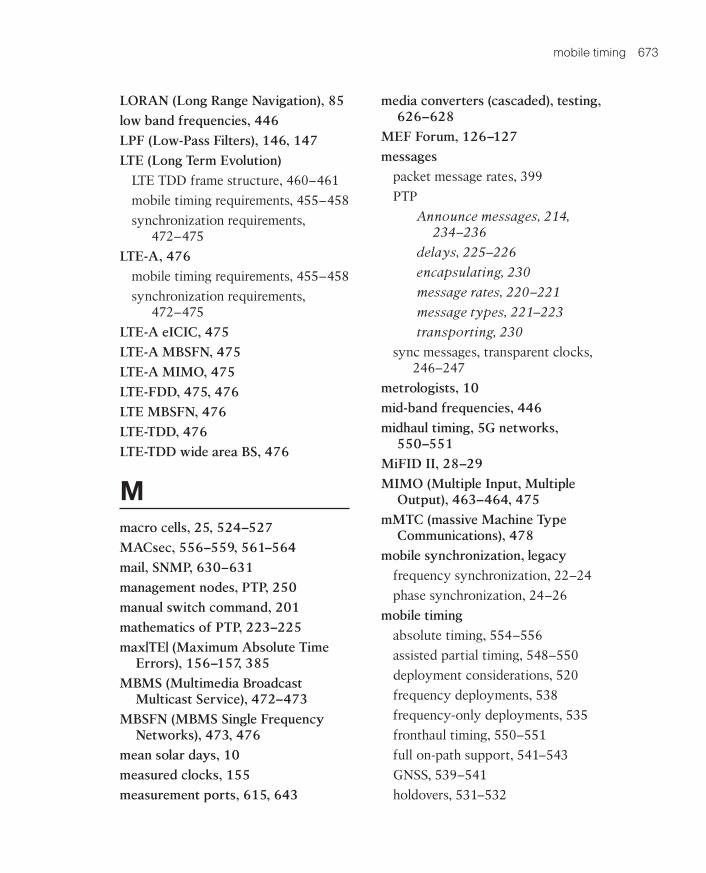
mobile timing 673
LORAN (Long Range Navigation), 85low band frequencies, 446LPF (Low-Pass Filters), 146, 147LTE (Long Term Evolution)
LTE TDD frame structure, 460–461mobile timing requirements, 455–458synchronization requirements,
472–475LTE-A, 476
mobile timing requirements, 455–458synchronization requirements,
472–475LTE-A eICIC, 475LTE-A MBSFN, 475LTE-A MIMO, 475LTE-FDD, 475, 476LTE MBSFN, 476LTE-TDD, 476LTE-TDD wide area BS, 476
Mmacro cells, 25, 524–527MACsec, 556–559, 561–564mail, SNMP, 630–631management nodes, PTP, 250manual switch command, 201mathematics of PTP, 223–225max|TE| (Maximum Absolute Time
Errors), 156–157, 385MBMS (Multimedia Broadcast
Multicast Service), 472–473MBSFN (MBMS Single Frequency
Networks), 473, 476mean solar days, 10measured clocks, 155measurement ports, 615, 643
media converters (cascaded), testing, 626–628
MEF Forum, 126–127messages
packet message rates, 399PTP
Announce messages, 214, 234–236
delays, 225–226encapsulating, 230message rates, 220–221message types, 221–223transporting, 230
sync messages, transparent clocks, 246–247
metrologists, 10mid-band frequencies, 446midhaul timing, 5G networks,
550–551MiFID II, 28–29MIMO (Multiple Input, Multiple
Output), 463–464, 475mMTC (massive Machine Type
Communications), 478mobile synchronization, legacy
frequency synchronization, 22–24phase synchronization, 24–26
mobile timingabsolute timing, 554–556assisted partial timing, 548–550deployment considerations, 520frequency deployments, 538frequency-only deployments, 535fronthaul timing, 550–551full on-path support, 541–543GNSS, 539–541holdovers, 531–532
9780136836254_print.indb 673 29/04/21 6:58 pm
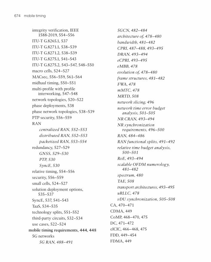
674 mobile timing
integrity verification, IEEE 1588-2019, 554–556
ITU-T G.8265.1, 537ITU-T G.8271.1, 538–539ITU-T G.8271.2, 538–539ITU-T G.8275.1, 541–543ITU-T G.8275.2, 543–547, 548–550macro cells, 524–527MACsec, 556–559, 561–564midhaul timing, 550–551multi-profile with profile
interworking, 547–548network topologies, 520–522phase deployments, 538phase network topologies, 538–539PTP security, 556–559RAN
centralized RAN, 552–553distributed RAN, 552–553packetized RAN, 553–554
redundancy, 527–529GNSS, 529–530PTP, 530SyncE, 530
relative timing, 554–556security, 556–559small cells, 524–527solution deployment options,
535–537SyncE, 537, 541–543TaaS, 534–535technology splits, 551–552third-party circuits, 532–534use cases, 522–524
mobile timing requirements, 444, 4485G networks
5G RAN, 488–491
5GCN, 482–484architecture of, 478–480bandwidth, 481–482CPRI, 487–488, 493–495DRAN, 493–494eCPRI, 493–495eMBB, 478evolution of, 478–480frame structures, 481–482FWA, 478mMTC, 478MRTD, 508network slicing, 496network time error budget
analysis, 501–505NR CRAN, 493–494NR synchronization
requirements, 496–500RAN, 484–486RAN functional splits, 491–492relative time budget analysis,
500–501RoE, 493–494scalable OFDM numerology,
481–482spectrum, 480TAE, 508transport architectures, 493–495uRLLC, 478vDU synchronization, 505–508
CA, 470–471CDMA, 449CoMP, 468–470, 475DC, 471–472eICIC, 466–468, 475FDD, 449–454FDMA, 449
9780136836254_print.indb 674 29/04/21 6:58 pm
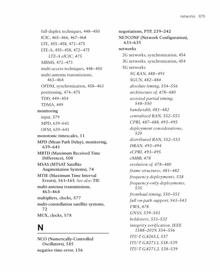
networks 675
full-duplex techniques, 448–450ICIC, 465–466, 467–468LTE, 455–458, 472–475LTE-A, 455–458, 472–475
LTE-A eICIC, 475MBMS, 472–473multi-access techniques, 448–450multi-antenna transmissions,
463–464OFDM, synchronization, 458–463positioning, 474–475TDD, 449–454TDMA, 449
monitoringinput, 579MPD, 639–641OFM, 639–641
monotonic timescales, 11MPD (Mean Path Delay), monitoring,
639–641MRTD (Maximum Received Time
Difference), 508MSAS (MTSAT Satellite
Augmentation Systems), 74MTIE (Maximum Time Interval
Errors), 161–165. See also TIEmulti-antenna transmissions,
463–464multipliers, clocks, 577multi-constellation satellite systems,
72MUX, clocks, 578
NNCO (Numerically-Controlled
Oscillators), 585negative time error, 156
negotiations, PTP, 239–242NETCONF (Network Configuration),
631–635networks
2G networks, synchronization, 4543G networks, synchronization, 4545G networks
5G RAN, 488–4915GCN, 482–484absolute timing, 554–556architecture of, 478–480assisted partial timing,
548–550bandwidth, 481–482centralized RAN, 552–553CPRI, 487–488, 493–495deployment considerations,
520distributed RAN, 552–553DRAN, 493–494eCPRI, 493–495eMBB, 478evolution of, 478–480frame structures, 481–482frequency deployments, 538frequency-only deployments,
535fronthaul timing, 550–551full on-path support, 541–543FWA, 478GNSS, 539–541holdovers, 531–532integrity verification, IEEE
1588–2019, 554–556ITU-T G.8265.1, 537ITU-T G.8271.1, 538–539ITU-T G.8271.2, 538–539
9780136836254_print.indb 675 29/04/21 6:58 pm
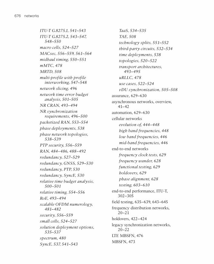
676 networks
ITU-T G.8275.1, 541–543ITU-T G.8275.2, 543–547,
548–550macro cells, 524–527MACsec, 556–559, 561–564midhaul timing, 550–551mMTC, 478MRTD, 508multi-profile with profile
interworking, 547–548network slicing, 496network time error budget
analysis, 501–505NR CRAN, 493–494NR synchronization
requirements, 496–500packetized RAN, 553–554phase deployments, 538phase network topologies,
538–539PTP security, 556–559RAN, 484–486, 488–492redundancy, 527–529redundancy, GNSS, 529–530redundancy, PTP, 530redundancy, SyncE, 530relative time budget analysis,
500–501relative timing, 554–556RoE, 493–494scalable OFDM numerology,
481–482security, 556–559small cells, 524–527solution deployment options,
535–537spectrum, 480SyncE, 537, 541–543
TaaS, 534–535TAE, 508technology splits, 551–552third-party circuits, 532–534time deployments, 538topologies, 520–522transport architectures,
493–495uRLLC, 478use cases, 522–524vDU synchronization, 505–508
assurance, 629–630asynchronous networks, overview,
41–42automation, 629–630cellular networks
evolution of, 444–448high band frequencies, 448low band frequencies, 446mid-band frequencies, 446
end-to-end networksfrequency clock tests, 629frequency wander, 628functional testing, 629holdovers, 629phase alignment, 628testing, 603–610
end-to-end performance, ITU-T, 302–305
field testing, 635–639, 643–645frequency distribution networks,
20–21holdovers, 422–424legacy synchronization networks,
20–22LTE MBSFN, 476MBSFN, 473
9780136836254_print.indb 676 29/04/21 6:58 pm
networks 677
mobile timing requirements, 444, 448CA, 470–471CDMA, 449CoMP, 468–470, 475DC, 471–472eICIC, 466–468FDD, 449–454FDMA, 449full-duplex techniques, 448–450ICIC, 465–466, 467–468LTE, 455–458, 472–475LTE-A, 455–458, 472–475MBMS, 472–473multi-access techniques,
448–450multi-antenna transmissions,
463–464OFDM, 458–463positioning, 474–475TDD, 449–454TDMA, 449
NETCONF, 631–635packet networks
ACR, 362–364CPRI, 487–488DCR, 364–365delay variations, 312–313frequencies, 359–369ITU-T G.8261, 310–312ITU-T G.8261.1, 312–313ITU-T G.8271.1, 323–325ITU-T G.8271.2, 325–326NTP, 365–366PTP, 366–369synchronization, 310–312time synchronization, 323–326timing, 310–312
packetstesting frequency clocks,
610–613topologies, 424–425transport networks, 426
performance, ITU-T G.8271, 322–323
RAN, 120–1215G RAN, 488–491, 551centralized RAN, 552–553distributed RAN, 552–553evolution of, 484–486functional splits, 491–492O-RAN Alliance, 122–124, 495packetized RAN, 553–554TIP OpenRAN, 125–126xRAN Forum, 122
SDH, 20–21slicing, 484, 496SNMP, 630–631SONET, 20–21synchronization network chains,
197–199synchronous networks, 40–41,
42–43TDM networks
AC, 31CEM, 30–32ITU-T recommendations, 298,
299–300slips, 22
telecommunications networksphase synchronization,
322–323time synchronization,
322–323time error budget analysis, 5G
networks, 501–505
9780136836254_print.indb 677 29/04/21 6:58 pm
678 networks
time synchronizationITU-T G.8271.1, 323–325ITU-T G.8271.2, 325–326
timing distribution networks, 82transport networks
carrying frequency, 426–428carrying phase/time, 428–430packet transport, 426–430
troubleshooting, 635–639active/passive probes, 641–643MFD monitoring, 639–641OFM monitoring, 639–641
TSG RAN, 107WAN, backup timing, 33–34YANG, 631–635
NIC, time sync, 505node clocks, ITU-T G.812, 306nodes
performance, 305–308, 326–328PTP-aware/unaware nodes,
374–376noise, 148–149, 165–166
clock nodes, 199generation, 167media converters (cascaded), testing,
627–628packets, 361, 384T-BC
noise generation, 405–406noise tolerance, 406–408noise transfer, 408–410testing, 616–617
T-BC-Anoise generation, 414noise tolerance, 414–415noise transfer, 414–415testing, 620–621
T-BC-Bnoise generation, 417–418noise tolerance, 418noise transfer, 418
T-BC-P testing, 622–623tolerance, 167–168transfers, 168–169transient events, 172transient response, 172T-TC, 413–414, 625–626T-TSC
noise generation, 405–406noise tolerance, 406–408noise transfer, 408–410testing, 616–617
T-TSC-Anoise generation, 414noise tolerance, 414–415noise transfer, 414–415testing, 620–621
T-TSC-Bnoise generation, 417–418noise tolerance, 418noise transfer, 418
T-TSC-P testing, 622–623nominal frequencies, 7non-mobile deployments, PTP,
430–431DOCSIS cable, 431–432power industry, 433–434remote PHY devices, 431–432
notes, ITU-T recommendations, 294–295
NR CRAN, 5G, 493–494NR synchronization requirements, 5G
networks, 496–500NSA (Non-Standalone Architectures),
482
9780136836254_print.indb 678 29/04/21 6:58 pm
packets 679
NTP (Network Time Protocol)packet networks, 365–366PTP vs, 215–216tine distribution network hierarchy,
28
OOAM (Open Application Model)
functions, 29ITU-T Series G Supplement 68, 340synchronization, 340
OCXO (Oven-Controlled Crystal Oscillators), 55, 56, 142
OFDM (Orthogonal Frequency-Division Multiplexing)
FDM vs, 455–457frame structures, 458–460scalable OFDM numerology,
5G networks, 481–482synchronization, 458
BS to BS synchronization, 462–463
cell search, 461frame structures, 458–460LTE TDD frame structure,
460–461UE to BS synchronization, 462
OFDMA, 455–458office clocks, 181OFM monitoring, 639–641one-step clocks, 230–231one-way PTP, 232–233O-RAN Alliance, 122–124, 495oscillators, 43–44, 140
aging, 56atomic oscillators, 55, 56–57cesium oscillators, 55–56
crystal oscillators, 141–142OCXO, 55, 56, 142TCXO, 55, 56, 142
free running oscillators, 41frequency, 44frequency counters, 44hydrogen masers, 56NCO, 585OCXO, 55, 56, 142PRC, 44–45quartz oscillators, 55rubidium oscillators, 55, 56signal histories, 170significant instants, 46–47TCXO, 55, 56, 142VCO, 143, 585VCXO, 142
overflow, data, 22
PP802.1ASdn, 634P1588e, 634packet clocks, 64–65
ITU-T G.8263, 327–328timing, 327–328
packet-only mode, PTP, 373–374packets
backhaul, frequency synchronization, 23–24
bandwidth, 361delay variations, 395–399distributions, time synchronization,
83, 87event messages, 48floor delay, 397–399frequencies
9780136836254_print.indb 679 29/04/21 6:58 pm
680 packets
clocks, testing, 610–613delivery, 319packet networks, 359–369packet-based distribution
performance, 383recommendations, creating, 310wander, 606–607
ITU-Tfrequency delivery, 319G.781.1, 318G.8260, 318–319G.8265, 319G.8265.1, 537synchronization definitions
and terminology, 318–319synchronization layer
functions, 318synchronization standards, 317timing recommendations,
316–317message rates, 399networks
ACR, 362–364CPRI, 487–488DCR, 364–365delay variations, 312–313ITU-T G.8261, 310–312ITU-T G.8261.1, 312–313ITU-T G.8271.1, 323–325ITU-T G.8271.2, 325–326NTP, 365–366PTP, 366–369synchronization, 310–312time synchronization, 323–325timing, 310–312topologies, 424–425
noise, 361performance
holdovers, 384noise, 384timing, 380, 383–385transient response, 384
phase distributions, 320–321, 370–372
processing, 584–586RAN, 553–554recommendations, ITU-T, 295–296regularity, 361selection process, 397–399synchronization, 48–49
definitions and terminology, 318–319
ITU-T G781.1, 318ITU-T G.8260, 318–319ITU-T G.8265, 319ITU-T standards, 317layer functions, 318
time distributions, 320–321, 370–372
timestamps, 48–49timing
ITU-T recommendations, 316–317
signals, 48–49traffic insensitivity, 361transport networks, 426
carrying frequency, 426–428carrying phase/time, 428–430
two-way TE, 400–401Paragon-neo, 595, 596Paragon-X, 595–596parent datasets, 237–238
9780136836254_print.indb 680 29/04/21 6:58 pm
phase 681
passive/active probes, 641–643PDU format, ESMC, 194–195peer-to-peer delay mechanisms, PTP,
231–232peer-to-peer transparent clocks,
248–249performance
clocks, 326–327, 401–402ITU-T G.8263, 327–328performance, ITU-T, 305–308synchronization chains, 62–64T-BC testing, 629T-TSC testing, 629
end-to-end performance, ITU-T, 302–305
ePRTC, 403–404networks, ITU-T G.8271, 322–323nodes, 326–327
ITU-T G.8263, 327–328performance, ITU-T, 305–308
packetsdistribution performance, 383holdovers, 384noise, 384timing, 380, 383–385transient response, 384
PRTC, 403–404periods, frequency, 43phase
5G network deployments, 538accuracy, 601alignment testing, 607–610carrying on transport networks,
428–430clocks
deviations, plot of, 149–152frameworks, 319–320
ITU-T G.8273, 319–320phase-aware clocks, 579–581
comparators, 143, 585delivery clock recommendations,
401–402deviations (clocks), plot of,
149–152end-to-end networks, 628errors, 155, 403frequency PLL, 576jitter, 602offset, 47packet distributions, 320–321, 372phase-aware clocks, 579–581phase recovery PLL, 576PTP inputs/outputs, 355–356satellite sources
BeiDou, 70Galileo, 70–71GLONASS, 69–70GNSS, 66–75GPS, 67–69IRNSS, 71multi-constellation satellite
systems, 72PRC, 66, 67, 75–78PRS, 66, 67, 75–78PRTC, 66, 67, 78–80QZSS, 71–72
synchronization, 7–9cable, 26–28clock offset, 47defined, 45–47frequency and phase alignment,
46legacy mobile synchronization,
24–26
9780136836254_print.indb 681 29/04/21 6:58 pm
682 phase
phase accuracy, 6phase offset, 47PON, 26–28relative offset, 47STB, 26–28telecom profiles, 336–338telecommunications networks,
322–323time synchronization versus, 6
system PLL, 576testing, 594, 607–610transients, 61, 63wander, 602
PHY devices (remote), 431–432physical layer distributions, time
synchronization, 83physical recommendations, ITU-T,
295–296, 299–300piezoelectric crystals, 141PIP (PTP Industry Profile), 263,
266–267plenaries, 293PLL (Phase-Locked Loops), 143–146,
152–153frequency PLL, 576phase recovery PLL, 576system PLL, 576T4 PLL, 576–577
plot of phase deviations, clocks, 149–152
PMU (Phasor Measurement Units), 33POC (Proof of Concept), 590PON, phase synchronization, 26–28ports
bundle of ports, 195datasets, 238defined, 65forced switch command, 201
lockout commands, 201manual switch command, 201measurement ports, 615, 643PTP ports, 218–219, 228–230virtual PTP ports, 239, 356–357
positioning, 474–475positive time error, 156power industry, non-mobile
deployments, 433–434power profile, 263, 268–269PRC (Primary Reference Clocks), 21,
44–45, 66, 67, 75–762-MHz frequency, 7710-MHz frequency, 76–77BITS, 77–78SSU, 77–78testing, 600–603
Preamble fields, 41precision, time, 15primary level SSU, 52primary reference clocks
ITU-T G.811, 306ITU-T G.811.1, 306–307
probes, active/passive, 641–643profile interworking, 5G networks,
547–548profiles, PTP, 250–251
AES67, 263, 269–270characteristics of major profiles,
261–263gPTP, 262–266PIP, 263, 266–267power profile, 263, 268–269PTP Enterprise Profile (RFC draft),
263, 270–272PUP, 263, 267–268SMPTE ST-2059–2, 263, 269–270
9780136836254_print.indb 682 29/04/21 6:58 pm
PTP (Precision Time Protocol) 683
telecom profiles, 252G.8265.1, 254–255G.8275.1, 255–257G.8275.2, 258–261
White Rabbit (WR), 263, 272–273proposals
ITU-T, 293POC, 590RFP, 587–590writing for, 587–590
protocol stacks, 584–585PRS (Primary Reference Sources), 21,
66, 67, 75–762-MHz frequency, 7710-MHz frequency, 76–77BITS, 77–78SSU, 77–78
PRTC (Primary Reference Time Clocks), 64, 65, 66, 67, 78–80, 403–404
1PSS, 80–81ePRTC, 403–404
ITU-T G.8272.1, 330–331timing, 330–331
testing, 600–603timing, 329–331ToD signals, 81–82
PTP (Precision Time Protocol), 29, 32–33, 64–65, 110–111
aBMCA, 236ACR, 362–364AES67, 263, 269–270Announce messages, 214, 234–236assisted partial timing support,
376–377asymmetry, 389
correction, 226–228correction/calibration, 392–395
dynamic asymmetry, 390–391message delays, 225–226static asymmetry, 389–390
aware/unaware nodes, 374–376BMCA, 236–237clockClass, 53clocks, 242–243
boundary clocks, 245–246domains, 220grandmaster (ordinary) clocks,
243–244overview, 218–219performance, 401–402slave (ordinary) clocks,
244–245testing standalone PTP clocks,
613–629transparent clocks, 246–249
correction field, 228cTE, 385–386datasets, 237–239DCR, 364–365delivery clocks, 401–402dTE, 386–388end-to-end delay mechanisms,
231–232end-to-end TE, 419–421ePRTC, 403–404frequency inputs/outputs, 349–350
BNC connectors, 350–351DIN 1.0/2.3 connectors, 350,
352QL, 354–355RJ-45 type connectors, 352–353SMB connectors, 350SyncE, 353–354
FTS, 372–373GNSS, 357–359
9780136836254_print.indb 683 29/04/21 6:58 pm
684 PTP (Precision Time Protocol)
gPTP, 114, 262–266hardware solution requirements,
574–575frequency synchronization
clocks, 577–579phase-aware clocks, 579–581PTP-aware clocks, 581–586SETS, 575–577time-aware clocks, 579–581
history of, 214hybrid mode, 373–374IEEE 1588, next steps, 279IEEE 1588–2008 (PTPv2),
216–217ITU-T
phase/time recommendations, 401–402
recommendations, 298–299leap seconds, 377–380management nodes, 250mathematics of, 223–225max|TE|385messages
delays, 225–226encapsulating, 230rates, 220–221transporting, 230types of, 221–223
negotiations, 239–242networks
holdovers, 422–424packet network topologies,
424–425transport networks, 426–430
non-mobile deployments, 430–431DOCSIS cable, 431–432power industry, 433–434remote PHY devices, 431–432
NTP vs, 215–216one-step clocks, 230–231one-way PTP, 232–233overview, 214
general overview, 217–218PTP clocks, 218–219
packet-only mode, 373–374packets
delay variations, 395–399floor delay, 397–399message rates, 399networks, 366–369networks, ACR, 362–364networks, DCR, 364–365networks, frequencies, 359–369networks, topologies, 424–425performance, 380performance, holdovers, 384performance, noise, 384performance, timing, 383–385performance, transient
response, 384phase distributions, 370–372selection process, 397–399time distributions, 370–372transport networks, 426–430two-way TE, 400–401
peer-to-peer delay mechanisms, 231–232
performanceclocks, 401–402packet-based distribution
performance, 383phase inputs/outputs, 355–356PIP, 263, 266–267ports, 218–219, 228–230
defined, 65virtual PTP ports, 239
9780136836254_print.indb 684 29/04/21 6:58 pm
PTP (Precision Time Protocol) 685
power profile, 263, 268–269profiles, 250–251
AES67, 263, 269–270characteristics of major
profiles, 261–263gPTP, 262–266PIP, 263, 266–267power profile, 263, 268–269PTP Enterprise Profile (RFC
draft), 263, 270–272PUP, 263, 267–268SMPTE ST-2059–2, 263,
269–270telecom profiles, 252–261White Rabbit (WR), 263,
272–273PRTC, 403–404PTP-aware clocks, 581
control plane processing, 584–586
hardware-assisted timestamping, 581–584
packet processing, 584–586servo processing, 584–586
PTP Enterprise Profile (RFC draft), 263, 270–272
PTPv2, 216–217, 629–630, 632–633PTPv2.1, 275–279PTS, 372–373PUP, 263, 267–268redundancy, 530security, 273–276, 556–559servo loops, 586SMPTE ST-2059–2, 263, 269–270software solution requirements,
574–575frequency synchronization
clocks, 577–579phase-aware clocks, 579–581
PTP-aware clocks, 581–586SETS, 575–577time-aware clocks, 579–581
synchronization types and timing, 348
TAI, 379–380T-BC, 404–405
holdovers, 411–412noise generation, 405–406noise tolerance, 406–408noise transfer, 408–410transient response, 410–411
T-BC-A, 414holdovers, 416–417noise generation, 414noise tolerance, 414–415noise transfer, 414–415transient response, 415
T-BC-B, 417holdovers, 419noise generation, 417–418noise tolerance, 418noise transfer, 418transient response, 418–419
telecom profiles, 217, 295–296time inputs/outputs, 355–356timescales, 233–234, 377–380timestamps, 233–234timing and synchronization types,
348T-TC, 413–414T-TSC, 404–405
holdovers, 411–412noise generation, 405–406noise tolerance, 406–408noise transfer, 408–410transient response, 410–411
9780136836254_print.indb 685 29/04/21 6:58 pm
686 PTP (Precision Time Protocol)
T-TSC-A, 414holdovers, 416–417noise generation, 414noise tolerance, 414–415noise transfer, 414–415transient response, 415
T-TSC-B, 417holdovers, 419noise generation, 417–418noise tolerance, 418noise transfer, 418transient response, 418–419
two-step clocks, 230–231two-way PTP, 232–233unicast negotiations, 239–242UTC, 379–380virtual PTP ports, 356–357White Rabbit (WR), 263, 272–273
PTS (Full Timing Support), 372–373pull-in range, 61, 63, 145–146pull-out range, 146PUP (Power Utility Automation
Profile), 263, 267–268
QQL (Quality Levels), clocks, 191–193,
354–355QL TLV format, ESMC, 195QL-disabled mode, clock selection
process, 200QL-enabled mode, clock selection
process, 200quality traceability, clocks, 51–53
clockClass, 53eESMC, 53ESMC, 53
health bits, 53methods, 53SSM bits, 52, 53time of day messages, 53timing loops, 54
quartz oscillators, 55question 13 (ITU-T study groups),
291–293QZSS (Global Navigation Satellite
System), 71–72
Rradio distribution systems, time
synchronization, 83, 84–86radios
CMDA radios, 24–25synchronization, 4
TDD radios, 25–26RAN (Radio Access Networks),
120–1215G RAN, 488–491, 551centralized RAN, 552–553DRAN, 493–494, 552–553evolution of, 484–486functional splits, 491–492O-RAN Alliance, 122–124, 495packetized RAN, 553–554positioning, 474–475TIP OpenRAN, 125–126xRAN Forum, 122
ranging, STB, 26–28rapporteurs, ITU-T, 293rearrangement of clocks, 201recommendations, ITU-T
creating, 293–294future of, 340–341
9780136836254_print.indb 686 29/04/21 6:58 pm
satellite sources of frequency, phase, and time 687
notes, 294–295packet recommendations, 295–296physical recommendations, 295–296,
299–300PTP
deployments, 298–299telecom profiles, 295–296
reading, 299TDM networks, 298, 299–300types of, 296–299
redundancy5G networks, 527–529
GNSS, 529–530PTP, 530SyncE, 530
GNSS, 529–530PTP, redundancy, 530SyncE, 530
reference receivers, 600reference signals, testing timing,
596–598regularity, packets, 361relative offset, 47relative time budget analysis, 5G
networks, 500–501relative timing, 554–556remote PHY devices, 431–432requests, writing for proposals,
587–590resonators, 43RFP (Request for Proposals),
587–590ring topologies, timing distributions,
202–206rise time, 47RJ-45 type connectors, 352–353RoE (Radio over Ethernet), 493–494
rollover, GPS, 647–648rubidium oscillators, 55, 56
SSA (Standalone Architectures), 482satellite sources of frequency, phase,
and timeBeiDou, 70Galileo, 70–71GLONASS, 69–70GNSS
augmentation systems, 72–75BeiDou, 70Galileo, 70–71GLONASS, 69–70GPS, 67–69IRNSS, 71multi-constellation satellite
systems, 72QZSS, 71–72
GNSS systems, 66–67GPS, 67–69IRNSS, 71multi-constellation satellite systems,
72PRC, 66, 67, 75–76
2-MHz frequency, 7710-MHz frequency, 76–77BITS, 77–78SSU, 77–78
PRS, 66, 67, 75–762-MHz frequency, 7710-MHz frequency, 76–77BITS, 77–78SSU, 77–78
PRTC, 66, 67, 78–80
9780136836254_print.indb 687 29/04/21 6:58 pm
688 satellite sources of frequency, phase, and time
1PSS, 80–81ToD signals, 81–82
QZSS, 71–72SBA (Service-Based Architectures),
483–484SBAS (Space-Based Augmentation
Systems), 72scalable OFDM numerology, 5G
networks, 481–482SC-FDMA, 455–458SDCM (System of Differential
Correction and Monitoring), 74SDH (Synchronous Digital
Hierarchies), 20–212-MHz frequency, 77SSM bits, 53
SDO (Standards Development Organizations), 97–98. See also standards
3GPP, 106–109AES, 128CPRI, 121–122ETSI, 116–117IEC, 115
IEC 62439–3, 115–116IEC/IEEE 60802, 116IEC/IEEE 61850, 116
IEEE, 109–110IEC and, 115–116IEC/IEEE 60802, 116IEC/IEEE 61850, 116PTP, 110–111
IETF, 118–120IMT, 104–106ITU, 98
ITU-D, 103, 290ITU-R, 99–100, 104, 290overview, 290
TSAG, 100WTSA, 100
ITU-T, 100–103, 290clock performance, 305–308consent, 294contributions, 293delegates, 293drafting, 294editors, 294end-to-end performance,
302–305end-to-end solutions, 322–326G.703, 309–310G.781, 300–302G.781.1, 318G.810, 302G.811, 306G.811.1, 306–307G.812, 307–308G.813, 308G.823, 303G.824, 303–304G.825, 304–305G.8260, 318–319G.8261, 310–312G.8261.1, 312–313G.8262, 314G.8262.1, 314–315G.8263, 327–328G.8264, 315–316G.8265, 319G.8265.1, 335–336, 537G.8266, 328–329G.8271, 322–323G.8271.1, 323–325, 538–539G.8271.2, 325–326, 538–539
9780136836254_print.indb 688 29/04/21 6:58 pm
servo processing 689
G.8272.1, 330–331G.8273, 319–320G.8273.1, 331G.8273.2, 331–332, 384,
613–618, 629G.8273.3, 332–333, 624–626G.8273.4, 333–334, 618–623G.8275, 320–321G.8275.1, 336–337, 541–543G.8275.2, 337–338, 543–547,
548–550GSTR-GNSS, 339–340interim meetings, 294network performance, 322–326node performance, 305–308packet recommendations,
295–296packet-based frequency
recommendations, 310–313packets, synchronization layer
functions, 318packets, synchronization
standards, 317packets, timing
recommendations, 316–317physical recommendations,
295–296, 299–300plenaries, 293proposals, 293PTP telecom profiles, 295–296question 13, 291–293rapporteurs, 293recommendations, creating,
293–294recommendations, future of,
340–341recommendations, notes,
294–295
recommendations, PTP deployments, 298–299
recommendations, reading, 299recommendations, types of,
296–299sector members, 293Series G Supplement 68, 340study groups, 291–293TDM networks, 298, 299–300working documents, 294
MEF Forum, 126–127O-RAN Alliance, 122–124RAN, 120–121
O-RAN Alliance, 122–124TIP OpenRAN, 125–126xRAN Forum, 122
SMPTE, 127–128TIP OpenRAN, 125–126TSAG, 100WTSA, 100xRAN Forum, 122
SEC (SDH Equipment Slave Clocks), ITU-T G.813, 308
sector members, 293security
integrity verification, IEEE 1588-2019, 554–556
MACsec, 556–559, 561–564PTP, 273–276, 556–559timing, 556–559
selection processclocks, 199–201packets, 397–399
Sentinel, 595, 644Series G Supplement 68, ITU-T, 340servo processing, 584–586
9780136836254_print.indb 689 29/04/21 6:58 pm
690 SETS (Synchronous Equipment Timing Source)
SETS (Synchronous Equipment Timing Source), 575–577
SG1, 103SG2, 100, 103SG3, 101SG5, 101SG9, 101SG11, 101SG15, 102SG16, 102SG17, 102signal histories, 170signal noise. See noisesignal strength, GNSS receivers,
645–647significant instants, 46–47slave (ordinary) clocks, 244–245
ITU-T G.812, 307–308SEC, ITU-T G.813, 308synchronous slave clocks
ITU-T G.8262, 314ITU-T G.8262.1, 314–315timing, 314–315
telecom time slave clocksITU-T G.8273.2, 331–332ITU-T G.8273.4, 333–334timing, 331–334
slicing networks, 484, 496slips, 22
defined, 22TDM networks, 22
small cells, 5G networks, 524–527SMB connectors, 350SMPTE (Society of Motion Picture
and Television Engineers), 127–128, 263
SNMP (Simple Network Mail Protocol), 630–631
software solution requirements, PTP, 574–575
frequency synchronization clocks, 577–579
phase-aware clocks, 579–581PTP-aware clocks, 581
control plane processing, 584–586
hardware-assisted timestamping, 581–584
packet processing, 584–586servo processing, 584–586
SETS, 575–577time-aware clocks, 579–581
SONET (Synchronous Optical Networking), 20–21
2-MHz frequency, 77SSM bits, 53
spatial diversity, 463spatial multiplexing, 464spoofing, GNSS, 541spreading codes, 449squelch, 53SSM, 87SSM (Synchronization Status
Messages), 191–193SSM bits, 52, 53SSU (Synchronization Supply Units),
52, 77–78, 181–185stability, time, 15standalone PTP clocks, testing, 613
T-BC, 613–618T-TSC, 613–618
standards, defined, 98. See also SDOstatic asymmetry, 389–390STB (Set-Top Boxes)
phase synchronization, 26–28ranging, 26–28
9780136836254_print.indb 690 29/04/21 6:58 pm
synchronization 691
stratum 1 clocks, 61stratum 2 clocks, 61stratum 3E clocks, 61stratum 4 clocks, 61stratum 4E clocks, 61stratum levels of frequency clocks,
59–61, 62–64study groups (ITU-T), 291–293sundials, 2sync messages, transparent clocks,
246–247SyncE (Synchronous Ethernet), 42
5G networks, 537, 541–543eESMC, 53ESMC, 53frequency
inputs/outputs, 353–354testing frequency wander,
604–607ITU-T G.8265.1, 537redundancy, 530
synchronization2G networks, 4543G networks, 454audiovisual synchronization, 32–33BS
BS to BS synchronization, 462–463
UE to BS synchronization, 462cell search, 461clock performance in
synchronization chains, 62–64defined, 3–4Ethernet, 53, 187–188, 193–195FDD, 450–454frequency synchronization, 7
aging, 7BITS, 181–185
clock selection process, 199–201
clock traceability, 189–191clocking hierarchy, 185–186clocks, 577–579eESMC, 196–197enhanced synchronous
Ethernet, 189ESMC, 193–195evolution of, 180–181frequency accuracy, 7legacy mobile synchronization,
22–24nominal frequencies, 7packet backhaul, 23–24SSM, 191–193SSU, 181–185synchronization network
chains, 197–199synchronous Ethernet, 187–188telecom profiles, 335–336time synchronization versus,
4–6timing loops, 195, 201–206
legacy mobile synchronizationfrequency synchronization,
22–24phase synchronization, 24–26
legacy synchronization networks, 20–22
LTE synchronization requirements, 472–475
LTE-A synchronization requirements, 472–475
mobile synchronization, legacyfrequency synchronization,
22–24phase synchronization, 24–26
network chains, 197–199
9780136836254_print.indb 691 29/04/21 6:58 pm
692 synchronization
NR synchronization requirements, 5G networks, 496–500
OAM, 340OFDM, 458
BS to BS synchronization, 462–463
cell search, 461frame structures, 458–460LTE TDD frame structure,
460–461UE to BS synchronization, 462
packet networks, timing, 310–312packet synchronization, 48–49
definitions and terminology, 318–319
ITU-T G781.1, 318ITU-T G.8260, 318–319ITU-T G.8265, 319ITU-T standards, 317layer functions, 318
phase synchronization, 7–9cable, 26–28clock offset, 47defined, 45–47frequency and phase alignment,
46legacy mobile synchronization,
24–26phase accuracy, 6phase offset, 47PON, 26–28relative offset, 47STB, 26–28telecom profiles, 336–338telecommunications networks,
322–323time synchronization versus, 6
primary level SSU, 52purpose of, 3–4radio synchronization, 4SSM, 191–193TDD, 450–454telecommunications, 20time of day synchronization,
9–10time synchronization, 6
consumers of, 88defined, 3–4frequency synchronization
versus, 4–6GNSS, 13–15GPS, 13–15ITU-T G.8271.1, 323–325ITU-T G.8271.2, 325–326overview, 1–3packet networks, 323–326packet-based distributions,
83, 87phase synchronization versus,
6physical layer distributions, 83radio distribution systems, 83,
84–86telecommunications networks,
322–323timing and synchronization types,
348UE to BS synchronization, 462vDU, 505–508
synchronous Ethernet, 313ITU-T G.8262, 314ITU-T G.8262.1, 314–315
synchronous networks, 40–41, 42–43
9780136836254_print.indb 692 29/04/21 6:58 pm
TE (Time Error) 693
synchronous slave clocksITU-T G.8262, 314ITU-T G.8262.1, 314–315timing, 314–315
synchrophasors, 33system PLL, 576
TT1 legacy circuits, 2-MHz frequency, 77T4 PLL, 576–577TaaS (Time as a Service), 534–535TAE (Time Alignment Errors), 508TAI (Temps Atomic International), 11,
379–380T-BC, 404–405
holdovers, 411–412noise generation, 405–406noise tolerance, 406–408noise transfer, 408–410testing, 613–618
clock performance, 629holdovers, 617noise, 616–617transient response, 617
transient response, 410–411T-BC-A, 414
holdovers, 416–417noise generation, 414noise tolerance, 414–415noise transfer, 414–415T-BC-A, noise, 620–621testing, 618–620
frequency accuracy, 620holdovers, 621transient response, 621
transient response, 415
T-BC-B, 417holdovers, 419noise generation, 417–418noise tolerance, 418noise transfer, 418transient response, 418–419
T-BC-P, testing, 621–622frequency accuracy, 622holdovers, 623noise, 622–623transient response, 623
TC (Transparent Clocks), 65TCXO (Temperature-Compensated
Crystal Oscillators), 55, 56, 142TDD (Time Division Duplexes),
449–450BS to BS synchronization, 462–463LTE TDD frame structure, 460–461LTE-TDD, 476LTE-TDD wide area BS, 476radios, 25–26, 463synchronization, 450–454UMTS-TDD, 2G/3G network
synchronization requirements, 454
TDEV (Time Deviation), 163–165TDM networks
AC, 31CEM, 30–32ITU-T recommendations, 298,
299–300slips, 22
TDMA (Time-Division Multiple Access), 449
TD-SCDMA, 2G/3G network synchronization requirements, 454
TE (Time Error), 154–156cTE, 160, 385–386
9780136836254_print.indb 693 29/04/21 6:58 pm
694 TE (Time Error)
dTE, 160–161, 386–388end-to-end TE, 419–421max|TE|156–157, 385measuring, 173–174MTIE. See also TIE, 161–165negative time error, 156network time error budget analysis,
5G networks, 501–505positive time error, 156TIE, 157–160. See also MTIEtwo-way TE, 400–401
technology splits, 5G networks, 551–552
telecom boundary clocksITU-T G.8273.2, 331–332ITU-T G.8273.4, 333–334timing, 331–332
telecom grandmaster clocks, 328–329, 331
telecom profiles, 217, 252, 334–335frequency synchronization, 335–336G.8265.1, 254–255G.8275.1, 255–257G.8275.2, 258–261ITU-T, 295–296ITU-T G.8265.1, 335–336ITU-T G.8275.1, 336–337ITU-T G.8275.2, 337–338phase synchronization, 336–338
telecom time slave clocks, 331–334telecom transparent clocks, 332–333telecommunications
networksphase synchronization,
322–323time synchronization, 322–323
synchronization, 20tempo. See frequency
TESLA (Timed Efficient Stream Loss-tolerant Authentication), 560
testingend-to-end networks, 603–610field testing, 635–639, 643–645frequency, 602–603frequency clocks in packet networks,
610–613frequency wander
packets, 606–607SyncE, 604–606
functional testing, end-to-end networks, 629
holdovers, 602media converters (cascaded),
626–628phase alignment, 607–610PRC, 600–603PRTC, 600–603PTP clocks, 613
T-BC, 613–618T-TSC, 613–618
T-BC, 613–618clock performance, 629holdovers, 613–618noise, 616–617transient response, 617
T-BC-A, 618–620frequency accuracy, 620holdovers, 621noise, 620–621transient response, 621
T-BC-P, 621–622frequency accuracy, 622holdovers, 623noise, 622–623transient response, 623
T-GM clocks, 600–603
9780136836254_print.indb 694 29/04/21 6:58 pm
time 695
timing, 603frequency, 602–603PRC, 600–603PRTC, 600–603T-GM clocks, 600–603
T-TC, 624–625holdovers, 626noise, 625–626transient response, 626
T-TSC, 613–618clock performance, 629holdovers, 613–618noise, 616–617transient response, 617
T-TSC-A, 618–620frequency accuracy, 620holdovers, 621noise, 620–621transient response, 621
T-TSC-P, 621–622frequency accuracy, 622holdovers, 623noise, 622–623transient response, 623
testing timing, 590–592calibration, 596–598frequency testing, 594overall approach, 592–594phase testing, 594reference signals, 596–598testing equipment, 595–596testing metrics, 599–600time testing, 594
T-GM clocks, testing, 600–603third-party circuits, 5G networks,
532–534
TIE (Time Interval Errors), 157–160. See also MTIE
time5G network deployments, 538accuracy, 15atomic clocks, 10, 11BIPM, 11carrying on transport networks,
428–430Coordinated Universal Time (UTC),
12–13cTE, 160, 385–386defined, 10–11delivery clock recommendations,
401–402dTE, 160–161, 386–388end-to-end TE, 419–421epochs, 11GMT, 3International Atomic Time (TAI), 11max|TE|156–157, 385mean solar days, 10metrologists, 10monotonic timescales, 11NTP, PTP vs, 215–216packet distributions, 320–321,
370–372precision, 15PTP, 29, 32–33
aBMCA, 236AES67, 263, 269–270Announce messages, 214,
234–236asymmetry, correction,
226–228asymmetry, message delays,
225–226BMCA, 236–237
9780136836254_print.indb 695 29/04/21 6:58 pm
696 time
boundary clocks, 245–246characteristics of major
profiles, 261–263clocks, 242–249clocks, domains, 220clocks, overview, 218–219correction field, 228datasets, 237–239encapsulating messages, 230end-to-end delay mechanisms,
231–232gPTP, 262–266grandmaster (ordinary) clocks,
243–244history of, 214IEEE 1588, next steps, 279IEEE 1588–2008 (PTPv2),
216–217inputs/outputs, 355–356management nodes, 250mathematics of, 223–225message delays, 225–226message rates, 220–221message types, 221–223negotiations, 239–242NTP vs, 215–216one-step clocks, 230–231one-way PTP, 232–233outputs/inputs, 355–356overview, 214overview, general overview,
217–218overview, PTP clocks, 218–219peer-to-peer delay mechanisms,
231–232PIP, 263, 266–267ports, 218–219, 228–230, 239
power profile, 263, 268–269profiles, 250–273PTP Enterprise Profile (RFC
draft), 263, 270–272PTPv2, 216–217PTPv2.1, 275–279PUP, 263, 267–268security, 273–276slave (ordinary) clocks,
244–245SMPTE ST-2059–2, 263,
269–270telecom profiles, 217, 252–261timescales, 233–234timestamps, 233–234transparent clocks, 246–249transporting messages, 230two-step clocks, 230–231two-way PTP, 232–233unicast negotiations, 239–242virtual PTP ports, 239White Rabbit (WR), 263,
272–273satellite sources
BeiDou, 70Galileo, 70–71GLONASS, 69–70GNSS, 67–75GNSS systems, 66–67GPS, 67–69IRNSS, 71multi-constellation satellite
systems, 72PRC, 66, 67, 75–78PRS, 66, 67, 75–78PRTC, 66, 67, 78–80QZSS, 71–72
9780136836254_print.indb 696 29/04/21 6:58 pm
timing 697
stability, 15sundials, 2synchronization, 6
defined, 3–4frequency synchronization
versus, 4–6GNSS, 13–15GPS, 13–15ITU-T G.8271.1, 323–325ITU-T G.8271.2, 325–326overview, 1–3packet networks, 323–326phase synchronization
versus, 6telecommunications networks,
322–323TAI, 11, 379–380testing, 594time-aware clocks, 579–581universal time (UT), 10UTC, 12–13, 379–380UTC(k), 12–13Zytturm (Clock Tower), 1–2
time clocks, frameworks, 319–320time distribution hierarchies,
frequency clocks, 62time error. See TEtime of day messages, 53time of day synchronization, 9–10time-power industry, industrial uses,
33–34time properties datasets, 238timescales, PTP, 233–234, 377–380timestamps
hardware-assisted timestamping, 581–584
packets, 48–49PTP, 233–234
time synchronizationconsumers of, 88NIC, 505packet-based distributions, 83, 87physical layer distributions, 83radio distribution systems, 83, 84–86
timingabsolute timing, 554–556distributions and ring topologies,
202–203ePRTC, 330–331ESMC, ITU-T G.8264, 315–316external timing, 182–183, 577fronthaul timing, 5G networks,
550–551FTS, 372–373integrity verification, IEEE 1588-
2019, 554–556ITU-T G.811, 306ITU-T G.811.1, 306–307ITU-T G.812, 306ITU-T G.813, 308line timing, 183–184line timing interfaces, 577loops, 195midhaul timing, 5G networks,
550–551mobile timing
absolute timing, 554–556assisted partial timing,
548–550centralized RAN, 552–553deployment considerations,
520distributed RAN, 552–553frequency deployments, 538frequency-only deployments,
535
9780136836254_print.indb 697 29/04/21 6:58 pm
698 timing
fronthaul timing, 550–551full on-path support, 541–543GNSS, 539–541holdovers, 531–532integrity verification, IEEE
1588–2019, 554–556ITU-T G.8265.1, 537ITU-T G.8271.1, 538–539ITU-T G.8271.2, 538–539ITU-T G.8275.1, 541–543ITU-T G.8275.2, 543–547,
548–550macro cells, 524–527MACsec, 556–559, 561–564midhaul timing, 550–551multi-profile with profile
interworking, 547–548network topologies, 520–522packetized RAN, 553–554phase deployments, 538phase network topologies,
538–539PTP security, 556–559redundancy, 527–529redundancy, GNSS, 529–530redundancy, PTP, 530redundancy, SyncE, 530relative timing, 554–556security, 556–559small cells, 524–527solution deployment options,
535–537SyncE, 537, 541–543TaaS, 534–535technology splits, 551–552third-party circuits, 532–534time deployments, 538use cases, 522–524
mobile timing requirements, 444, 4485G networks, 5G RAN,
488–4915G networks, 5GCN, 482–4845G networks, architecture of,
478–4805G networks, bandwidth,
481–4825G networks, CPRI, 487–488,
493–4955G networks, DRAN, 493–4945G networks, eCPRI, 493–4955G networks, eMBB, 4785G networks, evolution of,
478–4805G networks, frame structures,
481–4825G networks, FWA, 4785G networks, mMTC, 4785G networks, MRTD, 5085G networks, network slicing,
4965G networks, network time
error budget analysis, 501–505
5G networks, NR CRAN, 493–494
5G Networks, NR synchronization requirements, 496–500
5G networks, RAN, 484–4865G networks, RAN functional
splits, 491–4925G networks, relative time
budget analysis, 500–5015G networks, RoE, 493–4945G networks, scalable OFDM
numerology, 481–4825G networks, spectrum, 4805G networks, TAE, 508
9780136836254_print.indb 698 29/04/21 6:58 pm
timing signals 699
5G networks, transport architectures, 493–495
5G networks, uRLLC, 4785G networks, vDU
synchronization, 505–508CA, 470–471CDMA, 449CoMP, 468–470, 475DC, 471–472eICIC, 466–468FDD, 449–450FDD, synchronization, 450–
454FDMA, 449full-duplex techniques, 448–
450ICIC, 465–466, 467–468LTE, 455–458, 472–475LTE-A, 455–458, 472–475MBMS, 472–473multi-access techniques,
448–450multi-antenna transmissions,
463–464OFDM, 458–463positioning, 474–475TDD, 449–454TDMA, 449
packet clocks, 327–328packet networks
ITU-T G.8261, 310–312ITU-T G.8271.1, 323–325ITU-T G.8271.2, 325–326time synchronization, 323–326
packetsITU-T recommendations,
316–317performance, 380
performance, 383–385proposals
POC, 590RFP, 587–590writing requests for, 587–590
PRTC, 329–331PTP, assisted partial timing support,
376–377PTS, 372–373relative timing, 554–556security, 556–559SETS, 575–577synchronization types, 348synchronous slave clocks, 314–315telecom boundary clocks, 331–332telecom grandmaster clocks,
328–329, 331telecom transparent clocks, 332–333testing, 590–592, 603
calibration, 596–598frequency, 602–603frequency testing, 594overall approach, 592–594phase testing, 594PRC, 600–603PRTC, 600–603reference signals, 596–598testing equipment, 595–596testing metrics, 599–600T-GM clocks, 600–603time testing, 594
timing distribution networks, 82timing loops, 54, 201–206timing signals
jitter, 49–51packets, 48–49wander, 49–51
9780136836254_print.indb 699 29/04/21 6:58 pm
700 timing solutions, CEM
timing solutions, CEM, 31–32TIP OpenRAN, 125–126ToD errors, 403ToD signals, 81–82
phase inputs/outputs, 355–356time inputs/outputs, 355–356virtual PTP ports, 356–357
tolerance, noise, 167–168topologies
5G networks, 520–522packet networks, 424–425phase network topologies, 538–539
traceabilityclock quality traceability, 51–53clocks, 189–191defined, 52
traffic insensitivity, packets, 361transient events, 172transient response, 172
media converters (cascaded), testing, 628
packet performance, 384T-BC, 410–411T-BC testing, 617T-BC-A, 415T-BC-A testing, 621T-BC-B, 418–419T-BC-P testing, 623T-TC testing, 626T-TSC, 410–411T-TSC testing, 617T-TSC-A, 415T-TSC-A testing, 621T-TSC-B, 418–419T-TSC-P testing, 623
transparent clocks, 246
end-to-end transparent clocks, 247–248, 249
peer-to-peer transparent clocks, 248–249
transparent clocks, 246–247transport networks
carrying frequency, 426–428carrying phase/time, 428–430networks, packet network topologies,
426packets, transport networks, 426
transporting PTP message, 230troubleshooting networks, 635–639
active/passive probes, 641–643MFD monitoring, 639–641OFM monitoring, 639–641
TSAG (Telecommunication Standardization Advisory Group), 100
TSG CT (Core Network and Terminals), 107
TSG RAN (Radio Access Networks), 107
TSG SA (Service and System Aspects), 107
TSN (Time-Sensitive Networking), 111–115
T-TC, 413–414holdovers, 626noise, 625–626testing, 624–626transient response, 626
T-TSC, 404–405holdovers, 411–412noise generation, 405–406noise tolerance, 406–408noise transfer, 408–410
9780136836254_print.indb 700 29/04/21 6:58 pm
wander 701
testing, 613–618clock performance, 629holdovers, 613–618noise, 616–617transient response, 617
transient response, 410–411T-TSC-A, 414
holdovers, 416–417noise generation, 414noise tolerance, 414–415noise transfer, 414–415testing, 618–620
frequency accuracy, 620holdovers, 621noise, 620–621transient response, 621
transient response, 415T-TSC-B, 417
holdovers, 419noise generation, 417–418noise tolerance, 418noise transfer, 418transient response, 418–419
T-TSC-Pfrequency accuracy, 622holdovers, 623noise, 622–623testing, 621–623transient response, 623
two-step clocks, 230–231two-way PTP, 232–233two-way TE, 400–401
UUE to BS synchronization, 462UMTS-FDD, 2G/3G network
synchronization requirements, 454
UMTS-TDD, 2G/3G network synchronization requirements, 454
unaware/aware nodes, PTP, 374–376underflow, data, 22unicast negotiations, 239–242universal time (UT), 10uRLLC (ultra-Reliable and Low-
Latency Communication), 478use cases, 5G networks, 522–524UTC (Coordinated Universal Time),
12–13, 379–380UTC(k), 12–13
VVCO (Voltage-Controlled Oscillators),
143, 585VCXO (Voltage-Controlled Crystal
Oscillators), 142vDU, synchronization, 505–508verifying integrity, IEEE 1588–2019,
559–561virtual PTP ports, 239, 356–357
WWAAS (Wide Area Augmentation
Systems), 74WAN, backup timing, 33–34wander, 49–51, 61, 63, 146,
148–153end-to-end networks, 628frequency
packets, 606–607SyncE, 604–606
ITU-T G.823, 303ITU-T G.824, 303–304ITU-T G.825, 304–305phase wander, 602
9780136836254_print.indb 701 29/04/21 6:58 pm
702 warm-up time, clocks
warm-up time, clocks, 57WG1, 123WG2, 123–124WG3, 124WG4, 124WG5, 124WG6, 124WG7, 124WG8, 124WG9, 124White Rabbit (WR), 263, 272–273working documents, ITU-T, 294WP1, 102WP2, 102WP3, 102
WP5D (Working Party 5D), 104WTSA (World Telecommunication
Standardization Assembly), 100
XxRAN Forum, 122
YYANG (Yet Another Next Generation),
631–635
ZZytturm (Clock Tower), 1–2
9780136836254_print.indb 702 29/04/21 6:58 pm