synbreed: A Framework for the Analysis of GenomicPrediction Data using R

Valentin Wimmer

Plant BreedingTechnische Universitat Munchen

Gottingen, 28/29 March 2011

Plant Breeding 1

Outline

Day 1

Introduction to the synbreed package

Working with data class gpData

Current development status of synbreed package

Discussion

Day 2

Writing R extensions

R-Forge and SVN

Extending the synbreed package, common standards

Discussion and future work

Plant Breeding 2

Summary - synbreed package

Add-on for the open source environment for statistical computing R (RDevelopment Core Team 2010)

Title: Framework for the anaylsis of genomic prediction data using R

Version: 0.5-1

S3 class system (Chambers and Hastie 1992)

Hosted on R-Forge:https://r-forge.r-project.org/projects/synbreed/

SVN repository

Audience: Scientists and professionals

Package description in preparation for JSS

Plant Breeding 3

Objectives

1 Provide algorithms required in the analysis of genomic prediction data

2 Create a framework for the analysis using a unified data object resembling thestructure for a wide range of studies such as GS, GWAS or QTL mapping

3 Collection of methods within one open-source software package

4 Flexible implementation with respect to data structure, suitable for plant andanimal breeding

5 Gateway to other R packages with models for genomic prediction

Plant Breeding 4

Genomic selection

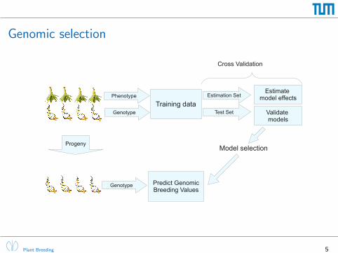
Phenotype

Genotype

Training dataEstimation Set

Test Set

Estimate model effects

Validate models

Progeny

Cross Validation

Genotype Predict GenomicBreeding Values

Model selection

Plant Breeding 5

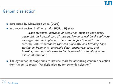
Genomic selection

Introduced by Meuwissen et al. (2001)

In a recent review, Heffner et al. (2009, p.9) state

“While statistical methods of prediction must be continuallyadvanced, an integral part of their performance will be the softwarepackages used to implement them. In conjunction with thissoftware, robust databases that can efficiently link breeding lines,testing environments, genotypic data, phenotypic data, andbreeding programs will need to be developed to simplify flow anduse of information.”

The synbreed package aims to provide tools for advancing genomic selectionfrom theory to praxis: “Analysis pipeline for genomic selection”

Plant Breeding 6

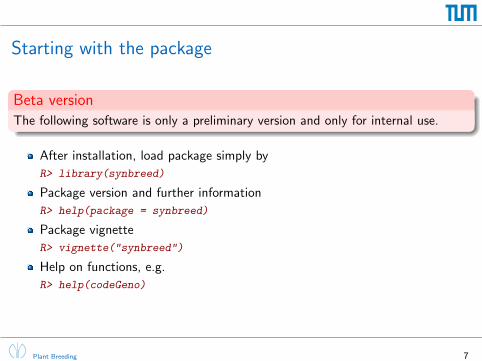
Starting with the package

Beta versionThe following software is only a preliminary version and only for internal use.

After installation, load package simply by

R> library(synbreed)

Package version and further information

R> help(package = synbreed)

Package vignette

R> vignette("synbreed")

Help on functions, e.g.

R> help(codeGeno)

Plant Breeding 7

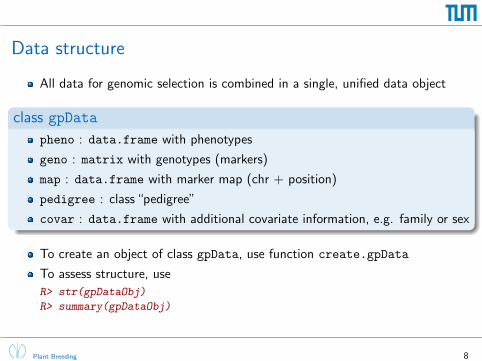
Data structure

All data for genomic selection is combined in a single, unified data object

class gpData

pheno : data.frame with phenotypes

geno : matrix with genotypes (markers)

map : data.frame with marker map (chr + position)

pedigree : class “pedigree”

covar : data.frame with additional covariate information, e.g. family or sex

To create an object of class gpData, use function create.gpData

To assess structure, use

R> str(gpDataObj)

R> summary(gpDataObj)

Plant Breeding 8

Data structure

Advantages of a unified data object

Common names for individuals and markers (like a data base)

Clear data queries and merges (like a data base)

Challenges: unphenotyped or ungenotyped individuals, markers withoutposition, additional individuals in pedigree

Only define data structure in the beginning, reuse for further analysis

Save all data in one Rdata object, considerably reduced storage requirement

All R scripts are based on the same data object (avoid missmatches)

Plant Breeding 9

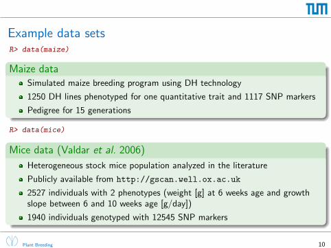
Example data setsR> data(maize)

Maize dataSimulated maize breeding program using DH technology

1250 DH lines phenotyped for one quantitative trait and 1117 SNP markers

Pedigree for 15 generations

R> data(mice)

Mice data (Valdar et al. 2006)

Heterogeneous stock mice population analyzed in the literature

Publicly available from http://gscan.well.ox.ac.uk

2527 individuals with 2 phenotypes (weight [g] at 6 weeks age and growthslope between 6 and 10 weeks age [g/day])

1940 individuals genotyped with 12545 SNP markers

Plant Breeding 10

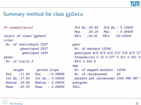
Summary method for class gpData

R> summary(mice)

object of class 'gpData'

covar

No. of individuals 2527

phenotyped 2527

genotyped 1940

pheno

No. of traits 2

weight growth.slope

Min. :11.90 Min. :-0.08889

1st Qu.:17.80 1st Qu.: 0.04556

Median :19.90 Median : 0.08024

Mean :20.30 Mean : 0.08659

3rd Qu.:22.60 3rd Qu.: 0.12569

Max. :30.20 Max. : 0.26408

NA's :16.00 NA's :53.00000

geno

No. of markers 12545

genotypes A/G G/G A/A C/C C/A A/T T/T G/C G/A C/G A/C T/A

frequencies 0.15 0.277 0.311 0.081 0.015 0.016 0.026 0.004 0.063 0.012 0.036 0.006

NA's 0.444 %

map

No. of mapped markers 12545

No. of chromosomes 20

markers per chromosome 1044 948 857 778 770 709 658 615 630 481 706 550 573 590 527 497 535 456 302 319

pedigree

NULL

Plant Breeding 11

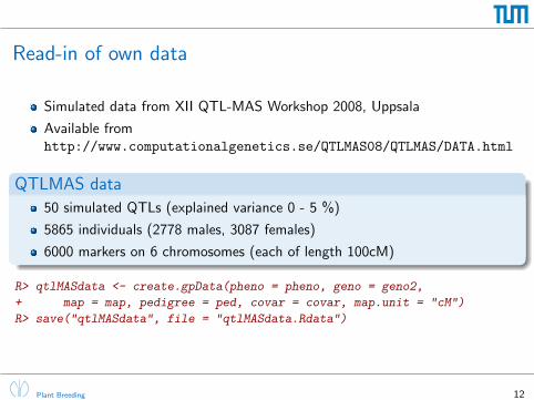
Read-in of own data

Simulated data from XII QTL-MAS Workshop 2008, Uppsala

Available fromhttp://www.computationalgenetics.se/QTLMAS08/QTLMAS/DATA.html

QTLMAS data

50 simulated QTLs (explained variance 0 - 5 %)

5865 individuals (2778 males, 3087 females)

6000 markers on 6 chromosomes (each of length 100cM)

R> qtlMASdata <- create.gpData(pheno = pheno, geno = geno2,

+ map = map, pedigree = ped, covar = covar, map.unit = "cM")

R> save("qtlMASdata", file = "qtlMASdata.Rdata")

Plant Breeding 12

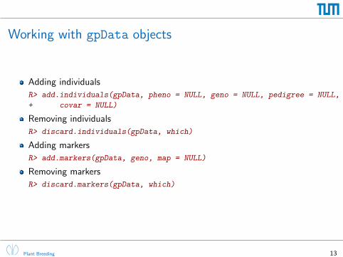
Working with gpData objects

Adding individuals

R> add.individuals(gpData, pheno = NULL, geno = NULL, pedigree = NULL,

+ covar = NULL)

Removing individuals

R> discard.individuals(gpData, which)

Adding markers

R> add.markers(gpData, geno, map = NULL)

Removing markers

R> discard.markers(gpData, which)

Plant Breeding 13

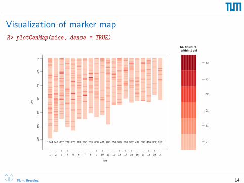
Visualization of marker mapR> plotGenMap(mice, dense = TRUE)

Nr. of SNPs within 1 cM

seq(

from

= 0

, to

= m

axD

ens,

leng

th =

6)

0

11

21

32

42

53

120

100

8060

4020

0

chr

pos

1 2 3 4 5 6 7 8 9 10 11 12 13 14 15 16 17 18 19 X

1044 948 857 778 770 709 658 615 630 481 706 550 573 590 527 497 535 456 302 319

Plant Breeding 14

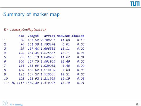
Summary of marker map

R> summaryGenMap(maize)

noM length avDist maxDist minDist

1 76 157.52 2.100267 11.08 0.10

2 96 151.38 1.593474 6.81 0.03

3 99 157.44 1.606531 13.11 0.02

4 122 154.34 1.275537 13.11 0.04

5 85 155.13 1.846786 11.67 0.01

6 106 157.70 1.501905 12.46 0.02

7 154 158.98 1.039085 6.48 0.02

8 130 156.62 1.214109 7.03 0.05

9 121 157.27 1.310583 14.21 0.06

10 128 153.92 1.211969 15.19 0.08

1 - 10 1117 1560.30 1.410027 15.19 0.01

Plant Breeding 15

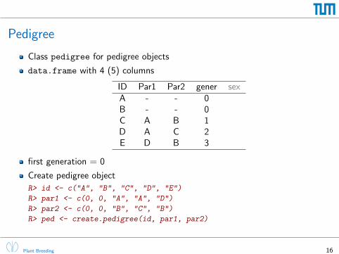
Pedigree

Class pedigree for pedigree objects

data.frame with 4 (5) columns

ID Par1 Par2 gener sexA - - 0B - - 0C A B 1D A C 2E D B 3

first generation = 0

Create pedigree object

R> id <- c("A", "B", "C", "D", "E")

R> par1 <- c(0, 0, "A", "A", "D")

R> par2 <- c(0, 0, "B", "C", "B")

R> ped <- create.pedigree(id, par1, par2)

Plant Breeding 16

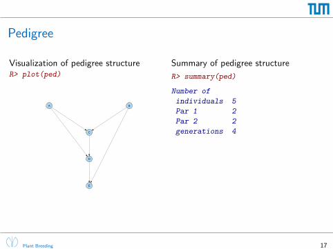
Pedigree

Visualization of pedigree structureR> plot(ped)

A B

C

D

E

Summary of pedigree structure

R> summary(ped)

Number of

individuals 5

Par 1 2

Par 2 2

generations 4

Plant Breeding 17

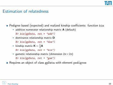
Estimation of relatedness

Pedigree based (expected) and realized kinship coefficients: function kinI additive numerator relationship matrix A (default)

R> kin(gpData, ret = "add")

I dominance relationship matrix D

R> kin(gpData, ret = "dom")

I kinship matrix K = 12A

R> kin(gpData, ret = "kin")

I gametic relationship matrix (dimension 2n×2n)

R> kin(gpData, ret = "gam")

Requires an object of class gpData with element pedigree

Plant Breeding 18

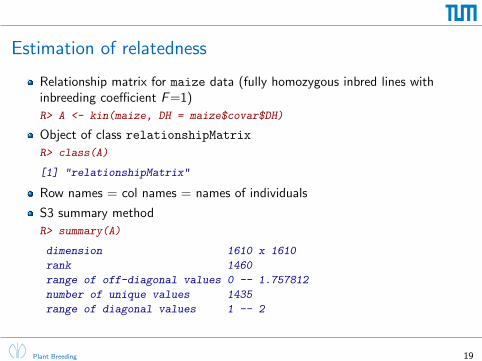
Estimation of relatedness

Relationship matrix for maize data (fully homozygous inbred lines withinbreeding coefficient F =1)

R> A <- kin(maize, DH = maize$covar$DH)

Object of class relationshipMatrix

R> class(A)

[1] "relationshipMatrix"

Row names = col names = names of individuals

S3 summary method

R> summary(A)

dimension 1610 x 1610

rank 1460

range of off-diagonal values 0 -- 1.757812

number of unique values 1435

range of diagonal values 1 -- 2

Plant Breeding 19

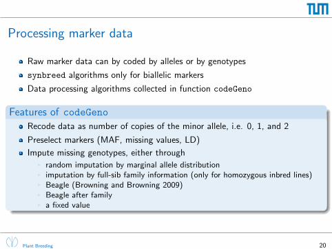
Processing marker data

Raw marker data can by coded by alleles or by genotypes

synbreed algorithms only for biallelic markers

Data processing algorithms collected in function codeGeno

Features of codeGenoRecode data as number of copies of the minor allele, i.e. 0, 1, and 2

Preselect markers (MAF, missing values, LD)

Impute missing genotypes, either throughI random imputation by marginal allele distributionI imputation by full-sib family information (only for homozygous inbred lines)I Beagle (Browning and Browning 2009)I Beagle after familyI a fixed value

Plant Breeding 20

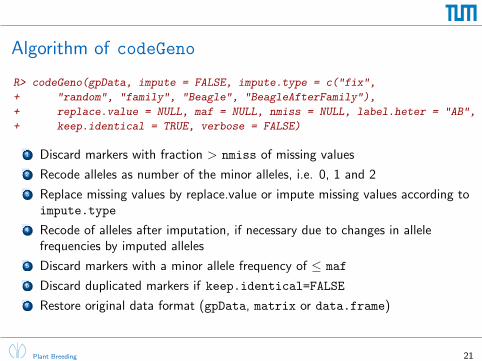
Algorithm of codeGeno

R> codeGeno(gpData, impute = FALSE, impute.type = c("fix",

+ "random", "family", "Beagle", "BeagleAfterFamily"),

+ replace.value = NULL, maf = NULL, nmiss = NULL, label.heter = "AB",

+ keep.identical = TRUE, verbose = FALSE)

1 Discard markers with fraction > nmiss of missing values

2 Recode alleles as number of the minor alleles, i.e. 0, 1 and 2

3 Replace missing values by replace.value or impute missing values according toimpute.type

4 Recode of alleles after imputation, if necessary due to changes in allelefrequencies by imputed alleles

5 Discard markers with a minor allele frequency of ≤ maf

6 Discard duplicated markers if keep.identical=FALSE

7 Restore original data format (gpData, matrix or data.frame)

Plant Breeding 21

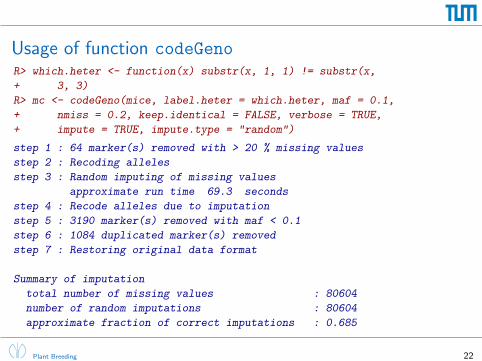
Usage of function codeGenoR> which.heter <- function(x) substr(x, 1, 1) != substr(x,

+ 3, 3)

R> mc <- codeGeno(mice, label.heter = which.heter, maf = 0.1,

+ nmiss = 0.2, keep.identical = FALSE, verbose = TRUE,

+ impute = TRUE, impute.type = "random")

step 1 : 64 marker(s) removed with > 20 % missing values

step 2 : Recoding alleles

step 3 : Random imputing of missing values

approximate run time 69.3 seconds

step 4 : Recode alleles due to imputation

step 5 : 3190 marker(s) removed with maf < 0.1

step 6 : 1084 duplicated marker(s) removed

step 7 : Restoring original data format

Summary of imputation

total number of missing values : 80604

number of random imputations : 80604

approximate fraction of correct imputations : 0.685

Plant Breeding 22

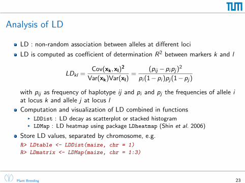
Analysis of LD

LD : non-random association between alleles at different loci

LD is computed as coefficient of determination R2 between markers k and l

LDkl =Cov(xk,xl)

2

Var(xk)Var(xl)=

(pij −pipj)2

pi (1−pi )pj(1−pj)

with pij as frequency of haplotype ij and pi and pj the frequencies of allele iat locus k and allele j at locus l

Computation and visualization of LD combined in functionsI LDDist : LD decay as scatterplot or stacked histogramI LDMap : LD heatmap using package LDheatmap (Shin et al. 2006)

Store LD values, separated by chromosome, e.g.

R> LDtable <- LDDist(maize, chr = 1)

R> LDmatrix <- LDMap(maize, chr = 1:3)

Plant Breeding 23

0 50 100 150

0.0

0.2

0.4

0.6

0.8

1.0

chromosome 1

dist [cM]

r2

(0,25] (25,50] (50,75] (75,160]

chromosome 1

dist [cM]

frac

tion

of S

NP

pai

rs

0.0

0.2

0.4

0.6

0.8

1.0

LD (r2)

(0,0.05](0.05,0.1](0.1,0.2](0.2,0.3](0.3,0.5](0.5,1]

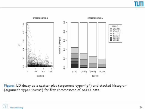
Figure: LD decay as a scatter plot (argument type="p") and stacked histogram(argument type="bars") for first chromosome of maize data.

Plant Breeding 24

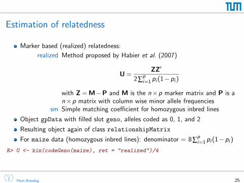
Estimation of relatedness

Marker based (realized) relatedness:

realized Method proposed by Habier et al. (2007)

U =ZZ′

2∑pi=1 pi (1−pi )

with Z = M−P and M is the n×p marker matrix and P is an×p matrix with column wise minor allele frequencies

sm Simple matching coefficient for homozygous inbred lines

Object gpData with filled slot geno, alleles coded as 0, 1, and 2

Resulting object again of class relationshipMatrix

For maize data (homozygous inbred lines): denominator = 8∑pi=1 pi (1−pi )

R> U <- kin(codeGeno(maize), ret = "realized")/4

Plant Breeding 25

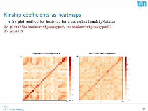
Kinship coefficients as heatmapsS3 plot method for heatmap for class relationshipMatrix

R> plot(A[maize$covar$genotyped, maize$covar$genotyped])

R> plot(U)

Plant Breeding 26

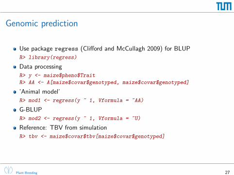
Genomic prediction

Use package regress (Clifford and McCullagh 2009) for BLUP

R> library(regress)

Data processing

R> y <- maize$pheno$Trait

R> AA <- A[maize$covar$genotyped, maize$covar$genotyped]

’Animal model’

R> mod1 <- regress(y ~ 1, Vformula = ~AA)

G-BLUP

R> mod2 <- regress(y ~ 1, Vformula = ~U)

Reference: TBV from simulation

R> tbv <- maize$covar$tbv[maize$covar$genotyped]

Plant Breeding 27

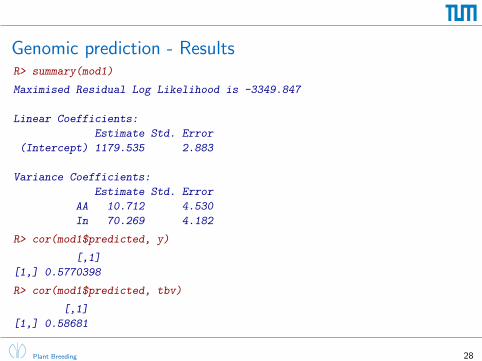
Genomic prediction - ResultsR> summary(mod1)

Maximised Residual Log Likelihood is -3349.847

Linear Coefficients:

Estimate Std. Error

(Intercept) 1179.535 2.883

Variance Coefficients:

Estimate Std. Error

AA 10.712 4.530

In 70.269 4.182

R> cor(mod1$predicted, y)

[,1]

[1,] 0.5770398

R> cor(mod1$predicted, tbv)

[,1]

[1,] 0.58681

Plant Breeding 28

Genomic prediction - ResultsR> summary(mod2)

Maximised Residual Log Likelihood is -3223.837

Linear Coefficients:

Estimate Std. Error

(Intercept) 1178.921 0.197

Variance Coefficients:

Estimate Std. Error

U 106.100 14.716

In 48.578 2.287

R> cor(mod2$predicted, y)

[,1]

[1,] 0.7264322

R> cor(mod2$predicted, tbv)

[,1]

[1,] 0.8563112

Plant Breeding 29

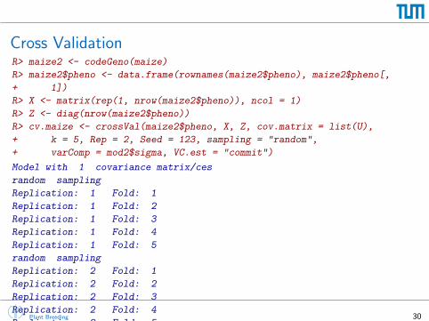
Cross ValidationR> maize2 <- codeGeno(maize)

R> maize2$pheno <- data.frame(rownames(maize2$pheno), maize2$pheno[,

+ 1])

R> X <- matrix(rep(1, nrow(maize2$pheno)), ncol = 1)

R> Z <- diag(nrow(maize2$pheno))

R> cv.maize <- crossVal(maize2$pheno, X, Z, cov.matrix = list(U),

+ k = 5, Rep = 2, Seed = 123, sampling = "random",

+ varComp = mod2$sigma, VC.est = "commit")

Model with 1 covariance matrix/ces

random sampling

Replication: 1 Fold: 1

Replication: 1 Fold: 2

Replication: 1 Fold: 3

Replication: 1 Fold: 4

Replication: 1 Fold: 5

random sampling

Replication: 2 Fold: 1

Replication: 2 Fold: 2

Replication: 2 Fold: 3

Replication: 2 Fold: 4

Replication: 2 Fold: 5Plant Breeding 30

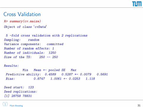
Cross ValidationR> summary(cv.maize)

Object of class 'cvData'

5 -fold cross validation with 2 replications

Sampling: random

Variance components: committed

Number of random effects: 1

Number of individuals: 1250

Size of the TS: 250 -- 250

Results:

Min Mean +- pooled SE Max

Predictive ability: 0.4589 0.5287 +- 0.0079 0.5691

Bias: 0.8747 1.0061 +- 0.0253 1.118

Seed start: 123

Seed replications:

[1] 28758 78831

Plant Breeding 31

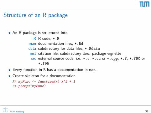
Structure of an R package

An R package is structured into

R R code, *.Rman documentation files, *.Rddata subdirectory for data files, *.Rdatainst citation file, subdirectory doc: package vignettesrc external source code, i.e. *.c, *.cc or *.cpp, *.f, *.f90 or

*.f95

Every function in R has a documentation in man

Create skeleton for a documentation

R> myFunc <- function(x) x^2 + 1

R> prompt(myFunc)

Plant Breeding 32

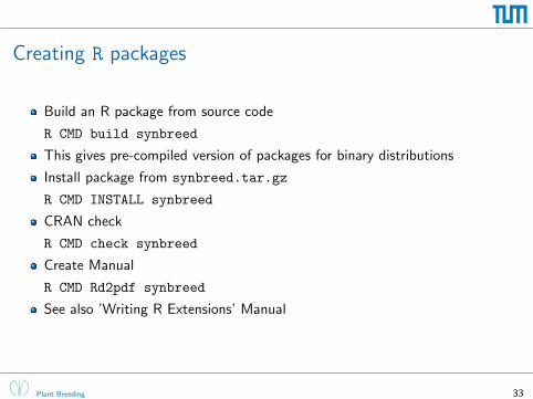
Creating R packages

Build an R package from source code

R CMD build synbreed

This gives pre-compiled version of packages for binary distributions

Install package from synbreed.tar.gz

R CMD INSTALL synbreed

CRAN check

R CMD check synbreed

Create Manual

R CMD Rd2pdf synbreed

See also ’Writing R Extensions’ Manual

Plant Breeding 33

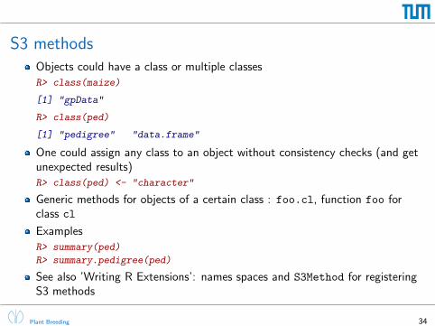
S3 methodsObjects could have a class or multiple classes

R> class(maize)

[1] "gpData"

R> class(ped)

[1] "pedigree" "data.frame"

One could assign any class to an object without consistency checks (and getunexpected results)

R> class(ped) <- "character"

Generic methods for objects of a certain class : foo.cl, function foo forclass cl

Examples

R> summary(ped)

R> summary.pedigree(ped)

See also ’Writing R Extensions’: names spaces and S3Method for registeringS3 methods

Plant Breeding 34

R-Forge

http://r-forge.r-project.org/

R-Forge is a subversion system for R package developers

Work is organized in ’Projects’

Source code management and version control

Authorized collaborators can ’check out’ or ’update’ the project file structure

SVN keeps track of the complete repository history

Package submission to CRAN

Plant Breeding 35

R-Forge

Automatic build from daily snapshot

Install packages from R-Forge

R> install.packages("synbreed", repos = "http://R-Forge.R-project.org")

No anonymous access at the moment

Roles in a project: Administrator, Senior developer, Junior developer

Additional features: Project website, mailing lists, project categorization,news, forums

For Synbreed: synbreed-news@lists.r-forge.r-project.org

More information on R-Forge in Theußl and Zeileis (2009)

Plant Breeding 36

SVN

Repositorysvn+ssh://username@svn.r-forge.r-project.org/svnroot/synbreed

More information on SVNhttp://svnbook.red-bean.com

SVN tool for Windowshttp://tortoisesvn.net/downloads

Plant Breeding 37

Future work

Stand-alone function for LD, additional measures, e.g. D ′

Imputation of missing genotypes: link to other software packages: Beagle

(Browning and Browning 2009) and/or fastPhase (Scheet and Stephens2006)

Genomic prediction methods, e.g. BayesA, BayesB (use external sourcecode?)

Simulation methods

Parallel computing

Data sets

. . .

Plant Breeding 38

Outlook

Package synbreed as framework for the analysis of breeding data

Promotion of own methods (citation in documentation)

Usage of a common data class

Guidelines for a collaborative software developmentI Common standards (S3 or S4)I Common example data setsI Standards for documentationI Quality checks (beyond R CMD check)

Plant Breeding 39

Dependencies for the synbreed package

To load the synbreed package, we require packages

lattice

igraph

MASS

LDheatmap

qtl

doBy

BLR

Plant Breeding 40

Gateway from synbreed to package qtl

Package qtl for QTL analysis in experimental crosses

Main data class cross

Conversion from gpData to cross

R> gpData2cross(gpDataObj)

Conversion from cross to gpData

R> cross2gpData(crossObj)

Plant Breeding 41

LiteratureBrowning, B. L., and S. R. Browning, 2009 A unified approach to genotype imputation and haplotype-phase

inference for large data sets of trios and unrelated individuals. The American Journal of Human Genetics846: 210–223.

Chambers, J. M., and T. J. Hastie, 1992 Statistical Models in S. Chapman & Hall. ISBN 9780412830402.

Clifford, D., and P. McCullagh, 2009 regress: Gaussian Linear Models with Linear Covariance Structure. Rpackage version 1.1-2.

Habier, D., R. Fernando, and J. Dekkers, 2007 The impact of genetic relationship information onGenome-Assisted breeding values. Genetics 177: 2389 – 2397.

Heffner, E. L., M. E. Sorrells, and J.-L. Jannink, 2009 Genomic selection for crop improvement. Crop Science49: 1–12.

Meuwissen, T. H. E., B. J. Hayes, and M. E. Goddard, 2001 Prediction of total genetic value usingGenome-Wide dense marker maps. Genetics 157: 1819–1829.

R Development Core Team, 2010 R: A Language and Environment for Statistical Computing . R Foundationfor Statistical Computing, Vienna, Austria.

Scheet, P., and M. Stephens, 2006 A fast and flexible statistical model for large-scale population genotypedata: Applications to inferring missing genotypes and haplotypic phase. The American Journal of HumanGenetics 78: 629–644.

Shin, J.-H., S. Blay, B. McNeney, and J. Graham, 2006 Ldheatmap: An R function for graphical display ofpairwise linkage disequilibria between single nucleotide polymorphisms. J Stat Soft 16: Code Snippet 3.

Theußl, S., and A. Zeileis, 2009 Collaborative Software Development Using R-Forge. The R Journal 1: 9–14.

Valdar, W., L. Solberg, D. Gauguier, W. Cookson, J. Rawlins, et al., 2006 Genetic and environmental effectson complex traits in mice. Genetics 174: 959–984.

Plant Breeding 42

Acknowledgement

Chris-Carolin Schon Henner Simianer Carsten Knaak Michael HohleHans-Jurgen Auinger Malena Erbe Milena Ouzunova Larry SchaefferTheresa Albrecht Richard Mottthe working group

This research was funded by the German Federal Ministry of Education

and Research (BMBF) within the AgroClustEr “Synbreed - Synergistic

plant and animal breeding” (Grant ID 0315528A).

Plant Breeding 43