Embed Size (px)
Citation preview
Available online at www.sciencedirect.com
Chaos, Solitons and Fractals 40 (2009) 2532–2543
www.elsevier.com/locate/chaos
Symplectic synchronization of different chaotic systems
Zheng-Ming Ge *, Cheng-Hsiung Yang
Department of Mechanical Engineering, National Chiao Tung University, Hsinchu 300, Taiwan, ROC
Accepted 29 October 2007
Communicated by Prof. Ji-Huan He
Abstract
In this paper, a new symplectic synchronization of chaotic systems is studied. Traditional generalized synchroniza-tions are special cases of the symplectic synchronization. A sufficient condition is given for the asymptotical stability ofthe null solution of an error dynamics. The symplectic synchronization may be applied to the design of secure commu-nication. Finally, numerical results are studied for a Quantum-CNN oscillators synchronized with a Rossler system inthree different cases.� 2007 Elsevier Ltd. All rights reserved.
1. Introduction
Many approaches have been presented for the synchronization of chaotic systems [2–6]. There are a chaotic mastersystem and either an identical or a different slave system. Our goal is the synchronization of the chaotic master and thechaotic slave by coupling or by other methods.
Among many kinds of synchronizations [7], generalized synchronization is investigated [8–12]. There exists a func-tional relationship between the states of the master and that of the slave. In this paper, a new synchronization
0960-0doi:10
* CoE-m
1 ThClassic
y ¼ Hðx; y; tÞ þ F ðtÞ ð1Þ
is studied, where x, y are the state vectors of the ‘‘master’’ and of the ‘‘slave’’, respectively, F(t) is a given function oftime in different form, such as a regular or a chaotic function. When H(x,y, t) = x, Eq. (1) reduces to the generalizedsynchronization given in [1]. Therefore this paper is an extension of [1].
In Eq. (1), the final desired state y of the ‘‘slave’’ system not only depends upon the ‘‘master’’ system state x but alsodepends upon the ‘‘slave’’ system state y itself. Therefore the ‘‘slave’’ system is not a traditional pure slave obeying the‘‘master’’ system completely but plays a role to determine the final desired state of the ‘‘slave’’ system. In other words, itplays an ‘‘interwined’’ role, so we call this kind of synchronization ‘‘symplectic synchronization’’1, and call the ‘‘master’’system partner A, the ‘‘slave’’ system partner B.
779/$ - see front matter � 2007 Elsevier Ltd. All rights reserved..1016/j.chaos.2007.10.055
rresponding author. Tel.: +886 3 5712121; fax: +886 3 5720634.ail address: [email protected] (Z.-M. Ge).
e term ‘‘symplectic’’ comes from the Greek for ‘‘interwined’’. H. Weyl first introduced the term in 1939 in his book ‘‘Theal Groups’’ (p. 165 in both the first edition, 1939, and second edition, 1946, Princeton University Press).
Z.-M. Ge, C.-H. Yang / Chaos, Solitons and Fractals 40 (2009) 2532–2543 2533
When H(x,y, t) = H(x, t), Eq. (1) becomes
y ¼ Hðx; tÞ þ F ðtÞ ð2Þ
which reduces to generalized synchronization. Therefore generalized synchronization is a special case of the symplecticsynchronization. There exists great potential of the application of the symplectic synchronization. For instance, whenthe symplectically synchronized chaotic signal is used as a signal carrier, the secure communication is more difficult tobe deciphered.
As numerical examples, recently developed Quantum Cellular Neural Network (Quantum-CNN) chaotic oscillatoris used to synchronize with different systems, respectively. Quantum-CNN oscillator equations are derived from aSchrodinger equation taking into account quantum dots cellular automata structures to which in the last decade a wideinterest has been devoted, with particular attention towards quantum computing [13].
This paper is organized as follows. In Section 2, by the Lyapunov asymptotical stability theorem, a symplectic syn-chronization scheme is given. In Section 3, various feedback controllers are designed for the symplectic synchronizationof the Quantum-CNN oscillator and a Rossler system. Numerical simulations are also given in Section 3. Finally, someconcluding remarks are given in Section 4.
2. Symplectic synchronization scheme
There are two different nonlinear chaotic systems. The partner A controls the partner B partially. The partner A isgiven by
_x ¼ f ðxÞ ð3Þ
where x = [x1,x2, . . . ,xn]T 2 Rn is a state vector and f is a vector function.The partner B is given by
_y ¼ gðyÞ ð4aÞ
where y = [y1,y2, . . . ,yn]T 2 Rn is a state vector, and g is a vector function different from f.After a controller u(t) is added, partner B becomes
_y ¼ gðyÞ þ uðtÞ ð4bÞ
where u(t) = [u1(t),u2(t), . . . ,un(t)]T 2 Rn is the control vector.Our goal is to design the controller u(t) so that the state vector y of the partner B asymptotically approaches
H(x,y, t) + F(t), a given function H(x,y, t) plus a given vector function F(t) = [F1(t),F2(t), . . . ,Fn(t)]T which is a regularor a chaotic function of time. Define error vector e(t) = [e1,e2, . . . ,en]T:
e ¼ Hðx; y; tÞ � y þ F ðtÞ ð5Þlimt!1
e ¼ 0 ð6Þ
is demanded.From Eq. (5), it is obtained that
_e ¼ oHox
_xþ oHoy
_y þ oHot� _y þ _F ðtÞ ð7Þ
By Eqs. (3), (4a) and (4b), (7) becomes
_e ¼ oHox
f ðxÞ þ oHoy
gðyÞ þ oHot� gðyÞ � uðtÞ þ _F ðtÞ ð8Þ
A positive definite Lyapnuov function V(e) is chosen:
V ðeÞ ¼ 1
2eTe ð9Þ
Its derivative along any solution of Eq. (8) is
_V ðeÞ ¼ eT oHox
f ðxÞ þ oHoy
gðyÞ þ oHot� gðyÞ þ _F ðtÞ � uðtÞ
� �: ð10Þ
In Eq. (10), u(t) is designed so that _V ¼ eTCn�ne where Cn·n is a diagonal negative definite matrix. _V is a negative def-inite function of e. By Lyapunov theorem of asymptotical stability
2534 Z.-M. Ge, C.-H. Yang / Chaos, Solitons and Fractals 40 (2009) 2532–2543
limt!1
e ¼ 0
The symplectic synchronization is obtained [14–16].
3. Numerical results for the symplectic chaos synchronization of Quantum-CNN oscillator and Rossler System
Case I: A cubic symplectic synchronization
For a two-cell Quantum-CNN, following differential equations are obtained [13]
_x1 ¼ �2a1
ffiffiffiffiffiffiffiffiffiffiffiffiffi1� x2
1
psin x2
_x2 ¼ �x1ðx1 � x3Þ þ 2a1x1ffiffiffiffiffiffiffiffiffiffiffiffiffi
1� x21
p cos x2
_x3 ¼ �2a2
ffiffiffiffiffiffiffiffiffiffiffiffiffi1� x2
3
psin x4
_x4 ¼ �x2ðx3 � x1Þ þ 2a2x3ffiffiffiffiffiffiffiffiffiffiffiffiffi
1� x23
p cos x4
8>>>>>>>><>>>>>>>>:
ð11Þ
where x1, x3 are polarizations, x2, x4 are quantum phase displacements, a1 and a2 are proportional to the inter-dotenergy inside each cell and x1 and x2 are the parameters that weigh the effects on the cell of the difference of polari-zation of the neighboring cells, like the cloning templates in traditional CNNs. When a1 = 19.4, a2 = 13.1, x1 = 9.529and x2 = 7.94, the system is chaotic.
A chaotic Rossler system is described by
_y1 ¼ �y2 � y3
_y2 ¼ y1 � ay2 þ y4
_y3 ¼ y1y3 þ b
_y4 ¼ cy3 þ ry4
8>>><>>>:
ð12Þ
where a = 0.5, b = 0.52, c = 0.5, r = 0.05.For symplectic synchronization of these two systems, u1, u2, u3 and u4 are added to the four equations of Eq. (12),
respectively:
_y1 ¼ �y2 � y3 þ u1
_y2 ¼ y1 � ay2 þ y4 þ u2
_y3 ¼ y1y3 þ bþ u3
_y4 ¼ cy3 þ ry4 þ u4
8>>><>>>:
ð13Þ
The initial values of the states of the Quantum-CNN system and of the Rossler system are taken as x1(0) = 0.8,x2(0) = �0.77, x3(0) = �0.72, x4(0) = 0.57, y1(0) = 0.3, y2(0) = �0.4, y3(0) = �0.7 and y4(0) = 0.15.
We take F 1ðtÞ ¼ x34ðtÞ, F 2ðtÞ ¼ x3
1ðtÞ, F 3ðtÞ ¼ x32ðtÞ, and F 4ðtÞ ¼ x3
3ðtÞ. They are chaotic functions of time.H iðx; y; tÞ ¼ �x2
i yi ði ¼ 1; 2; 3; 4Þ are given. By Eq. (6) we have
limt!1
ei ¼ limt!1ð�x2
i yi � yi þ x3j Þ ¼ 0; i ¼ 1; 2; 3; 4 j ¼
4; i ¼ 1
i� 1; i–1
�ð14Þ
From Eq. (7) we have
_ei ¼ �2 _xixiyi � x2i _yi � _yi þ 3 _xjx2
j ; i ¼ 1; 2; 3; 4 j ¼4; i ¼ 1
i� 1; i–1
�ð15Þ
Eq. (8) can be expressed as
_e1 ¼ 2y1x1 2a1
ffiffiffiffiffiffiffiffiffiffiffiffiffi1� x2
1
qsin x2
� �þ ðy2 þ y3Þx2
1 þ y2 þ y3 � u1
þ 3x24 �x2ðx3 � x1Þ þ 2a2
x3ffiffiffiffiffiffiffiffiffiffiffiffiffi1� x2
3
p cos x4
!
Z.-M. Ge, C.-H. Yang / Chaos, Solitons and Fractals 40 (2009) 2532–2543 2535
_e2 ¼ �2y2x2 �x1ðx1 � x3Þ þ 2a1x1ffiffiffiffiffiffiffiffiffiffiffiffiffi
1� x21
p cos x2
!� ðy1 � ay2 þ y4Þx2
2
� y1 þ ay2 � y4 � u2 þ 3x21 �2a1
ffiffiffiffiffiffiffiffiffiffiffiffiffi1� x2
1
qsin x2
� �
_e3 ¼ 2y3x3 2a2
ffiffiffiffiffiffiffiffiffiffiffiffiffi1� x2
3
qsin x4
� �� ðy1y3 þ bÞx3
2 � y1y3 � b� u3
þ 3x22 �x1ðx1 � x3Þ þ 2a1
x1ffiffiffiffiffiffiffiffiffiffiffiffiffi1� x2
1
p cos x2
!
_e4 ¼ �2y4x4 �x2ðx3 � x1Þ þ 2a2x3ffiffiffiffiffiffiffiffiffiffiffiffiffi
1� x23
p cos x4
!� ðcy3 þ ry4Þx2
4 � cy3
� ry4 � u4 þ 3x23 �2a2
ffiffiffiffiffiffiffiffiffiffiffiffiffi1� x2
3
qsin x4
� �
where e1 ¼ �x21y1 � y1 þ x3
4, e2 ¼ �x22y2 � y2 þ x3
1, e3 ¼ �x23y3 � y3 þ x3
2 and e4 ¼ �x24y4 � y4 þ x3
3.Choose a positive definite Lyapunov function:
V ðe1; e2; e3; e4Þ ¼1
2ðe2
1 þ e22 þ e2
3 þ e24Þ ð17Þ
Its time derivative along any solution of Eq. (16) is
_V ¼ e1
(2y1x1 2a1
ffiffiffiffiffiffiffiffiffiffiffiffiffi1� x2
1
qsin x2
� �þ ðy2 þ y3Þx2
1 þ y2 þ y3
þ3x24 �x2ðx3 � x1Þ þ 2a2
x3ffiffiffiffiffiffiffiffiffiffiffiffiffi1� x2
3
p cos x4
!� u1
)
þ e2 �2y2x2 �x1ðx1 � x3Þ þ 2a1x1ffiffiffiffiffiffiffiffiffiffiffiffiffi
1� x21
p cos x2
!� ðy1 � ay2 þ y4Þx2
2
(
�y1 þ ay2 � y4 þ 3x21 �2a1
ffiffiffiffiffiffiffiffiffiffiffiffiffi1� x2
1
qsin x2
� �� u2
)
þ e3
(2y3x3 2a2
ffiffiffiffiffiffiffiffiffiffiffiffiffi1� x2
3
qsin x4
� �� ðy1y3 þ bÞx3
2 � y1y3 � b
þ3x22 �x1ðx1 � x3Þ þ 2a1
x1ffiffiffiffiffiffiffiffiffiffiffiffiffi1� x2
1
p cos x2
!� u3
)
þ e4 �2y4x4 �x2ðx3 � x1Þ þ 2a2x3ffiffiffiffiffiffiffiffiffiffiffiffiffi
1� x23
p cos x4
!� ðcy3 þ ry4Þx2
4 � cy3
(
�ry4 þ 3x23 �2a2
ffiffiffiffiffiffiffiffiffiffiffiffiffi1� x2
3
qsin x4
� �� u4
)
ð18Þ
Choose
u1 ¼ 2y1x1 2a1
ffiffiffiffiffiffiffiffiffiffiffiffiffi1� x2
1
qsin x2
� �þ ðy2 þ y3Þx2
1 þ y2 þ y3
þ 3x24 �x2ðx3 � x1Þ þ 2a2
x3ffiffiffiffiffiffiffiffiffiffiffiffiffi1� x2
3
p cos x4
!� y1x2
1 � y1 þ x34
u2 ¼ �2y2x2 �x1ðx1 � x3Þ þ 2a1
x1ffiffiffiffiffiffiffiffiffiffiffiffiffi1� x2
1
p cos x2
!� ðy1 � ay2 þ y4Þx2
2
� y1 � y4 þ 3x21 �2a1
ffiffiffiffiffiffiffiffiffiffiffiffiffi1� x2
1
qsin x2
� �� aðy2x2
2 � x31Þ
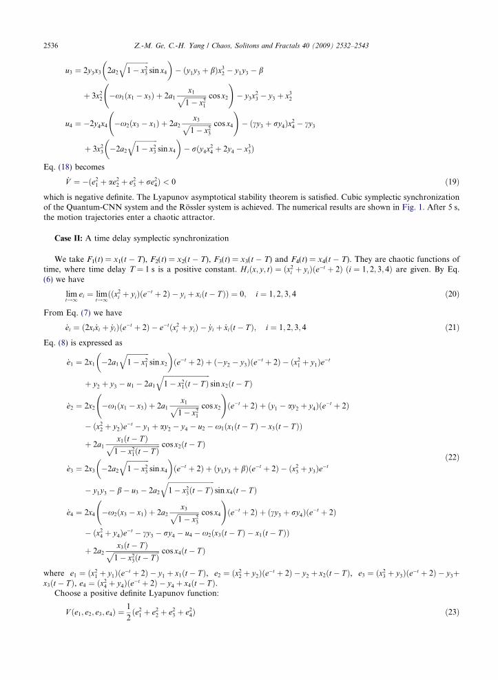
2536 Z.-M. Ge, C.-H. Yang / Chaos, Solitons and Fractals 40 (2009) 2532–2543
u3 ¼ 2y3x3 2a2
ffiffiffiffiffiffiffiffiffiffiffiffiffi1� x2
3
qsin x4
� �� ðy1y3 þ bÞx3
2 � y1y3 � b
þ 3x22 �x1ðx1 � x3Þ þ 2a1
x1ffiffiffiffiffiffiffiffiffiffiffiffiffi1� x2
1
p cos x2
!� y3x2
3 � y3 þ x32
u4 ¼ �2y4x4 �x2ðx3 � x1Þ þ 2a2
x3ffiffiffiffiffiffiffiffiffiffiffiffiffi1� x2
3
p cos x4
!� ðcy3 þ ry4Þx2
4 � cy3
þ 3x23 �2a2
ffiffiffiffiffiffiffiffiffiffiffiffiffi1� x2
3
qsin x4
� �� rðy4x2
4 þ 2y4 � x33Þ
Eq. (18) becomes
_V ¼ �ðe21 þ ae2
2 þ e23 þ re2
4Þ < 0 ð19Þ
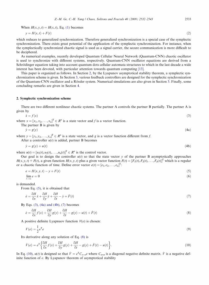
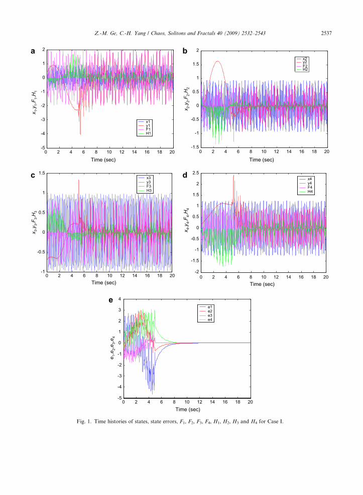
which is negative definite. The Lyapunov asymptotical stability theorem is satisfied. Cubic symplectic synchronizationof the Quantum-CNN system and the Rossler system is achieved. The numerical results are shown in Fig. 1. After 5 s,the motion trajectories enter a chaotic attractor.
Case II: A time delay symplectic synchronization
We take F1(t) = x1(t � T), F2(t) = x2(t � T), F3(t) = x3(t � T) and F4(t) = x4(t � T). They are chaotic functions oftime, where time delay T = 1 s is a positive constant. H iðx; y; tÞ ¼ ðx2
i þ yiÞðe�t þ 2Þ ði ¼ 1; 2; 3; 4Þ are given. By Eq.(6) we have
limt!1
ei ¼ limt!1ððx2
i þ yiÞðe�t þ 2Þ � yi þ xiðt � T ÞÞ ¼ 0; i ¼ 1; 2; 3; 4 ð20Þ
From Eq. (7) we have
_ei ¼ ð2xi _xi þ _yiÞðe�t þ 2Þ � e�tðx2i þ yiÞ � _yi þ _xiðt � T Þ; i ¼ 1; 2; 3; 4 ð21Þ
Eq. (8) is expressed as
_e1 ¼ 2x1 �2a1
ffiffiffiffiffiffiffiffiffiffiffiffiffi1� x2
1
qsin x2
� �ðe�t þ 2Þ þ ð�y2 � y3Þðe�t þ 2Þ � ðx2
1 þ y1Þe�t
þ y2 þ y3 � u1 � 2a1
ffiffiffiffiffiffiffiffiffiffiffiffiffiffiffiffiffiffiffiffiffiffiffiffiffiffiffi1� x2
1ðt � T Þq
sin x2ðt � T Þ
_e2 ¼ 2x2 �x1ðx1 � x3Þ þ 2a1x1ffiffiffiffiffiffiffiffiffiffiffiffiffi
1� x21
p cos x2
!ðe�t þ 2Þ þ ðy1 � ay2 þ y4Þðe�t þ 2Þ
� ðx22 þ y2Þe�t � y1 þ ay2 � y4 � u2 � x1ðx1ðt � T Þ � x3ðt � T ÞÞ
þ 2a1
x1ðt � T Þffiffiffiffiffiffiffiffiffiffiffiffiffiffiffiffiffiffiffiffiffiffiffiffiffiffiffi1� x2
1ðt � T Þp cos x2ðt � T Þ
_e3 ¼ 2x3 �2a2
ffiffiffiffiffiffiffiffiffiffiffiffiffi1� x2
3
qsin x4
� �ðe�t þ 2Þ þ ðy1y3 þ bÞðe�t þ 2Þ � ðx2
3 þ y3Þe�t
� y1y3 � b� u3 � 2a2
ffiffiffiffiffiffiffiffiffiffiffiffiffiffiffiffiffiffiffiffiffiffiffiffiffiffiffi1� x2
3ðt � T Þq
sin x4ðt � T Þ
_e4 ¼ 2x4 �x2ðx3 � x1Þ þ 2a2x3ffiffiffiffiffiffiffiffiffiffiffiffiffi
1� x23
p cos x4
!ðe�t þ 2Þ þ ðcy3 þ ry4Þðe�t þ 2Þ
� ðx24 þ y4Þe�t � cy3 � ry4 � u4 � x2ðx3ðt � T Þ � x1ðt � T ÞÞ
þ 2a2x3ðt � T Þffiffiffiffiffiffiffiffiffiffiffiffiffiffiffiffiffiffiffiffiffiffiffiffiffiffiffi
1� x23ðt � T Þ
p cos x4ðt � T Þ
ð22Þ
where e1 ¼ ðx21 þ y1Þðe�t þ 2Þ � y1 þ x1ðt � T Þ, e2 ¼ ðx2
2 þ y2Þðe�t þ 2Þ � y2 þ x2ðt � T Þ, e3 ¼ ðx23 þ y3Þðe�t þ 2Þ � y3þ
x3ðt � T Þ, e4 ¼ ðx24 þ y4Þðe�t þ 2Þ � y4 þ x4ðt � T Þ.
Choose a positive definite Lyapunov function:
V ðe1; e2; e3; e4Þ ¼1
2ðe2
1 þ e22 þ e2
3 þ e24Þ ð23Þ
0 2 4 6 8 10 12 14 16 18 20-2
-1.5
-1
-0.5
0
0.5
1
1.5
2
2.5x4y4F4H4
x 4,y
4,F4,H
4
0 2 4 6 8 10 12 14 16 18 20-1
-0.5
0
0.5
1
1.5x3y3F3H3
x 3,y
3,F3,H
3
0 2 4 6 8 10 12 14 16 18 20-5
-4
-3
-2
-1
0
1
2
3
4
e1e2e3e4
e 1,e
2,e3,e
4
Time (sec)
Time (sec) Time (sec)
Time (sec) Time (sec) 0 2 4 6 8 10 12 14 16 18 20
-5
-4
-3
-2
-1
0
1
2
x1y1F1H1
x 1,y
1,F1,H
1
0 2 4 6 8 10 12 14 16 18 20-1.5
-1
-0.5
0
0.5
1
1.5
2
x2y2F2H2
x 2,y
2,F2,H
2
a b
c d
e
Fig. 1. Time histories of states, state errors, F1, F2, F3, F4, H1, H2, H3 and H4 for Case I.
Z.-M. Ge, C.-H. Yang / Chaos, Solitons and Fractals 40 (2009) 2532–2543 2537
2538 Z.-M. Ge, C.-H. Yang / Chaos, Solitons and Fractals 40 (2009) 2532–2543
Its time derivative along any solution of Eq. (22) is
_V ¼ e1 2x1 �2a1
ffiffiffiffiffiffiffiffiffiffiffiffiffi1� x2
1
qsin x2
� �ðe�t þ 2Þ þ ð�y2 � y3Þðe�t þ 2Þ � ðx2
1 þ y1Þe�t
�
þy2 þ y3 � 2a1
ffiffiffiffiffiffiffiffiffiffiffiffiffiffiffiffiffiffiffiffiffiffiffiffiffiffiffi1� x2
1ðt � T Þq
sin x2ðt � T Þ � u1
�
þ e2 2x2 �x1ðx1 � x3Þ þ 2a1x1ffiffiffiffiffiffiffiffiffiffiffiffiffi
1� x21
p cos x2
!ðe�t þ 2Þ þ ðy1 � ay2 þ y4Þðe�t þ 2Þ � ðx2
2 þ y2Þe�t
(
�y1 þ ay2 � y4 � x1ðx1ðt � T Þ � x3ðt � T ÞÞ þ 2a1x1ðt � T Þffiffiffiffiffiffiffiffiffiffiffiffiffiffiffiffiffiffiffiffiffiffiffiffiffiffiffi
1� x21ðt � T Þ
p cos x2ðt � T Þ � u2
)
þ e3 2x3 �2a2
ffiffiffiffiffiffiffiffiffiffiffiffiffi1� x2
3
qsin x4
� �ðe�t þ 2Þ þ ðy1y3 þ bÞðe�t þ 2Þ � ðx2
3 þ y3Þe�t
�
�y1y3 � b� 2a2
ffiffiffiffiffiffiffiffiffiffiffiffiffiffiffiffiffiffiffiffiffiffiffiffiffiffiffi1� x2
3ðt � T Þq
sin x4ðt � T Þ � u3
�
þ e4 2x4 �x2ðx3 � x1Þ þ 2a2x3ffiffiffiffiffiffiffiffiffiffiffiffiffi
1� x23
p cos x4
!ðe�t þ 2Þ þ ðcy3 þ ry4Þðe�t þ 2Þ � ðx2
4 þ y4Þe�t
(
�cy3 � ry4 � x2ðx3ðt � T Þ � x1ðt � T ÞÞ þ 2a2x3ðt � T Þffiffiffiffiffiffiffiffiffiffiffiffiffiffiffiffiffiffiffiffiffiffiffiffiffiffiffi
1� x23ðt � T Þ
p cos x4ðt � T Þ � u4
)
ð24Þ
Choose
u1 ¼ 2x1 �2a1
ffiffiffiffiffiffiffiffiffiffiffiffiffi1� x2
1
qsin x2
� �ðe�t þ 2Þ þ ð�y2 � y3Þðe�t þ 2Þ � ðx2
1 þ y1Þe�t þ y2 þ y3
� 2a1
ffiffiffiffiffiffiffiffiffiffiffiffiffiffiffiffiffiffiffiffiffiffiffiffiffiffiffi1� x2
1ðt � T Þq
sin x2ðt � T Þ þ ðx21 þ y1Þðe�t þ 2Þ � y1 þ x1ðt � T Þ
u2 ¼ 2x2 �x1ðx1 � x3Þ þ 2a1x1ffiffiffiffiffiffiffiffiffiffiffiffiffi
1� x21
p cos x2
!ðe�t þ 2Þ þ ðy1 � ay2 þ y4Þðe�t þ 2Þ � ðx2
2 þ y2Þe�t
� y1 � y4 � x1ðx1ðt � T Þ � x3ðt � T ÞÞ þ 2a1
x1ðt � T Þffiffiffiffiffiffiffiffiffiffiffiffiffiffiffiffiffiffiffiffiffiffiffiffiffiffiffi1� x2
1ðt � T Þp cos x2ðt � T Þ
þ aððx22 þ y2Þðe�t þ 2Þ þ x2ðt � T ÞÞ
u3 ¼ 2x3 �2a2
ffiffiffiffiffiffiffiffiffiffiffiffiffi1� x2
3
qsin x4
� �ðe�t þ 2Þ þ ðy1y3 þ bÞðe�t þ 2Þ � ðx2
3 þ y3Þe�t
� y1y3 � b� 2a2
ffiffiffiffiffiffiffiffiffiffiffiffiffiffiffiffiffiffiffiffiffiffiffiffiffiffiffi1� x2
3ðt � T Þq
sin x4ðt � T Þ þ ðx23 þ y3Þðe�t þ 2Þ � y3 þ x3ðt � T Þ
u4 ¼ 2x4 �x2ðx3 � x1Þ þ 2a2
x3ffiffiffiffiffiffiffiffiffiffiffiffiffi1� x2
3
p cos x4
!ðe�t þ 2Þ þ ðcy3 þ ry4Þðe�t þ 2Þ � ðx2
4 þ y4Þe�t
� cy3 � x2ðx3ðt � T Þ � x1ðt � T ÞÞ þ 2a2x3ðt � T Þffiffiffiffiffiffiffiffiffiffiffiffiffiffiffiffiffiffiffiffiffiffiffiffiffiffiffi
1� x23ðt � T Þ
p cos x4ðt � T Þ
þ rððx24 þ y4Þðe�t þ 2Þ � 2y4 þ x4ðt � T ÞÞ
Eq. (24) becomes
_V ¼ �ðe21 þ ae2
2 þ e23 þ re2
4Þ < 0 ð25Þ
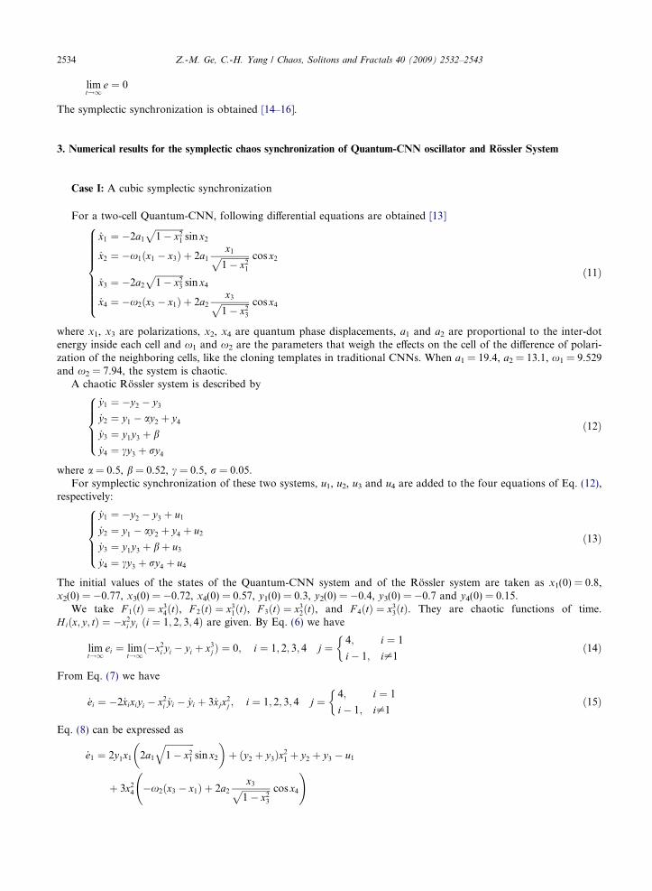
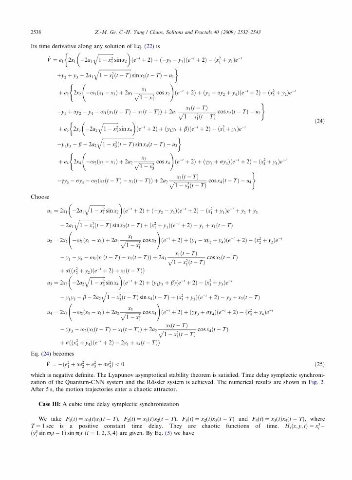
which is negative definite. The Lyapunov asymptotical stability theorem is satisfied. Time delay symplectic synchroni-zation of the Quantum-CNN system and the Rossler system is achieved. The numerical results are shown in Fig. 2.After 5 s, the motion trajectories enter a chaotic attractor.
Case III: A cubic time delay symplectic synchronization
We take F1(t) = x4(t)x1(t � T), F2(t) = x1(t)x2(t � T), F3(t) = x2(t)x3(t � T) and F4(t) = x3(t)x4(t � T), whereT = 1 sec is a positive constant time delay. They are chaotic functions of time. H iðx; y; tÞ ¼ x3
i�ðy3
i sin -it � 1Þ sin -it ði ¼ 1; 2; 3; 4Þ are given. By Eq. (5) we have
0 2 4 6 8 10 12 14 16 18 20-8
-6
-4
-2
0
2
4
6
x1y1F1H1
x 1,y
1,F1,H
1
0 2 4 6 8 10 12 14 16 18 20-3
-2
-1
0
1
2
3
4
5
6
x2y2F2H2
0 2 4 6 8 10 12 14 16 18 20-6
-4
-2
0
2
4
6x4y4F4H4
0 2 4 6 8 10 12 14 16 18 20-4
-3
-2
-1
0
1
2
3
4
5
6
x3y3F3H3
x 3,y
3,F3,H
3
x 4,y
4,F4,H
4x 2
,y2,F
2,H2
0 2 4 6 8 10 12 14 16 18 20-4
-3
-2
-1
0
1
2
3
4
5
6
e1e2e3e4
e 1,e
2,e3,e
4
Time (sec)
Time (sec) Time (sec)
Time (sec) Time (sec)
a b
c d
e
Fig. 2. Time histories of states, state errors, F1, F2, F3, F4, H1, H2, H3 and H4 for Case II.
Z.-M. Ge, C.-H. Yang / Chaos, Solitons and Fractals 40 (2009) 2532–2543 2539
limt!1
ei ¼ limt!1ðx3
i � ðy3i sin -it � 1Þ sin -it � yi þ xjxiðt � T ÞÞ ¼ 0; i ¼ 1; 2; 3; 4; j ¼
4; i ¼ 1
i� 1; i–1
�ð26Þ
2540 Z.-M. Ge, C.-H. Yang / Chaos, Solitons and Fractals 40 (2009) 2532–2543
From Eq. (7) we have
_ei ¼ ð3 _xix2i � ð3 _yiy2
i sin -it þ y3i -i cos -itÞ sin -it � ðy3
i sin -it � 1Þ-i cos -it � _yi þ _xjxiðt � T Þ þ xj _xiðt � T Þ;
i ¼ 1; 2; 3; 4; j ¼4; i ¼ 1
i� 1; i–1
�ð27Þ
Eq. (8) is expressed as
_e1 ¼ 3x21 �2a1
ffiffiffiffiffiffiffiffiffiffiffiffiffi1� x2
1
qsin x2
� �� 3y2
1ð�y2 � y3Þ sin2 -1t � y31-1 sin 2-1t
þ -1 cos -1t þ y2 þ y3 � u1 þ �x2ðx3 � x1Þ þ 2a2
x3ffiffiffiffiffiffiffiffiffiffiffiffiffi1� x2
3
p cos x4
!x1ðt � T Þ
� 2a1x4
ffiffiffiffiffiffiffiffiffiffiffiffiffiffiffiffiffiffiffiffiffiffiffiffiffiffiffi1� x2
1ðt � T Þq
sin x2ðt � T Þ
_e2 ¼ 3x22 �x1ðx1 � x3Þ þ 2a1
x1ffiffiffiffiffiffiffiffiffiffiffiffiffi1� x2
1
p cos x2
!� 3y2
2ðy1 � ay2 þ y4Þ sin2 -2t
� y32-2 sin 2-2t þ -2 cos -2t � y1 þ ay2 � y4 � u2 � 2a1x2ðt � T Þ
ffiffiffiffiffiffiffiffiffiffiffiffiffi1� x2
1
qsin x2
þ x1ð�x1ðx1ðt � T Þ � x3ðt � T ÞÞ þ 2a1x1ðt � T Þffiffiffiffiffiffiffiffiffiffiffiffiffiffiffiffiffiffiffiffiffiffiffiffiffiffiffi
1� x21ðt � T Þ
p cos x2ðt � T Þ
_e3 ¼ 3x23 �2a2
ffiffiffiffiffiffiffiffiffiffiffiffiffi1� x2
3
qsin x4
� �� 3y2
3ðy1y3 þ bÞ sin2 -3t þ y33-3 sin 2-3t
þ -3 cos -3t � y1y3 � b� u3 þ �x1ðx1 � x3Þ þ 2a1x1ffiffiffiffiffiffiffiffiffiffiffiffiffi
1� x21
p cos x2
!x3ðt � T Þ
� 2a2x2
ffiffiffiffiffiffiffiffiffiffiffiffiffiffiffiffiffiffiffiffiffiffiffiffiffiffiffi1� x2
3ðt � T Þq
sin x4ðt � T Þ
_e4 ¼ 3x24 �x2ðx3 � x1Þ þ 2a2
x3ffiffiffiffiffiffiffiffiffiffiffiffiffi1� x2
3
p cos x4
!� 3y2
4ðcy3 þ ry4Þ sin2 -4t
þ y34-4 sin 2-4t þ -4 cos -4t � cy3 � ry4 � u4 � 2a2x4ðt � T Þ
ffiffiffiffiffiffiffiffiffiffiffiffiffi1� x2
3
qsin x4
þ x3 �x2ðx3ðt � T Þ � x1ðt � T ÞÞ þ 2a2
x3ðt � T Þffiffiffiffiffiffiffiffiffiffiffiffiffiffiffiffiffiffiffiffiffiffiffiffiffiffiffi1� x2
3ðt � T Þp cos x4ðt � T Þ
!
ð28Þ
where
e1 ¼ x31 � ðy3
1 sin -1t � 1Þ sin -1t � y1 þ x4ðtÞx1ðt � T Þe2 ¼ x3
2 � ðy32 sin -2t � 1Þ sin -2t � y2 þ x1ðtÞx2ðt � T Þ
e3 ¼ x33 � ðy3
3 sin -3t � 1Þ sin -3t � y3 þ x2ðtÞx3ðt � T Þe4 ¼ x3
4 � ðy34 sin -4t � 1Þ sin -4t � y4 þ x3ðtÞx4ðt � T Þ
Choose a positive definite Lyapunov function:
V ðe1; e2; e3; e4Þ ¼1
2ðe2
1 þ e22 þ e2
3 þ e24Þ ð29Þ
Its time derivative along any solution of Eq. (28) is
_V ¼ e1 3x21 �2a1
ffiffiffiffiffiffiffiffiffiffiffiffiffi1� x2
1
qsin x2
� �� 3y2
1ð�y2 � y3Þ sin2 -1t � y31-1 sin 2-1t þ -1 cos -1t þ y2 þ y3
(
þ �x2ðx3 � x1Þ þ 2a2x3ffiffiffiffiffiffiffiffiffiffiffiffiffi
1� x23
p cos x4
!x1ðt � T Þ � 2a1x4
ffiffiffiffiffiffiffiffiffiffiffiffiffiffiffiffiffiffiffiffiffiffiffiffiffiffiffi1� x2
1ðt � T Þq
sin x2ðt � T Þ � u1
)
þ e2 3x22 �x1ðx1 � x3Þ þ 2a1
x1ffiffiffiffiffiffiffiffiffiffiffiffiffi1� x2
1
p cos x2
!� 3y2
2ðy1 � ay2 þ y4Þ sin2 -2t � y32-2 sin 2-2t
(
Z.-M. Ge, C.-H. Yang / Chaos, Solitons and Fractals 40 (2009) 2532–2543 2541
þ-2 cos -2t � y1 þ ay2 � y4 � 2a1x2ðt � T Þffiffiffiffiffiffiffiffiffiffiffiffiffi1� x2
1
qsin x2 þ x1ð�x1ðx1ðt � T Þ � x3ðt � T ÞÞ
þ2a1x1ðt � T Þffiffiffiffiffiffiffiffiffiffiffiffiffiffiffiffiffiffiffiffiffiffiffiffiffiffiffi
1� x21ðt � T Þ
p cos x2ðt � T Þ � u2
)
þ e3
(3x2
3 �2a2
ffiffiffiffiffiffiffiffiffiffiffiffiffi1� x2
3
qsin x4
� �� 3y2
3ðy1y3 þ bÞ sin2 -3t þ y33-3 sin 2-3t þ -3 cos -3t � y1y3
�bþ �x1ðx1 � x3Þ þ 2a1x1ffiffiffiffiffiffiffiffiffiffiffiffiffi
1� x21
p cos x2
!x3ðt � T Þ � 2a2x2
ffiffiffiffiffiffiffiffiffiffiffiffiffiffiffiffiffiffiffiffiffiffiffiffiffiffiffi1� x2
3ðt � T Þq
sin x4ðt � T Þ � u3
)
þ e4 3x24 �x2ðx3 � x1Þ þ 2a2
x3ffiffiffiffiffiffiffiffiffiffiffiffiffi1� x2
3
p cos x4
!� 3y2
4ðcy3 þ ry4Þ sin2 -4t þ y34-4 sin 2-4t
(
þ-4 cos -4t � cy3 � ry4 � 2a2x4ðt � T Þffiffiffiffiffiffiffiffiffiffiffiffiffi1� x2
3
qsin x4 þ x3ð�x2ðx3ðt � T Þ � x1ðt � T ÞÞ
þ2a2
x3ðt � T Þffiffiffiffiffiffiffiffiffiffiffiffiffiffiffiffiffiffiffiffiffiffiffiffiffiffiffi1� x2
3ðt � T Þp cos x4ðt � T ÞÞ � u4
)
Choose
u1 ¼ 3x21 �2a1
ffiffiffiffiffiffiffiffiffiffiffiffiffi1� x2
1
qsin x2
� �� 3y2
1ð�y2 � y3Þ sin2 -1t � y31-1 sin 2-1t
þ -1 cos -1t þ y2 þ y3 þ �x2ðx3 � x1Þ þ 2a2x3ffiffiffiffiffiffiffiffiffiffiffiffiffi
1� x23
p cos x4
!x1ðt � T Þ
� 2a1x4
ffiffiffiffiffiffiffiffiffiffiffiffiffiffiffiffiffiffiffiffiffiffiffiffiffiffiffi1� x2
1ðt � T Þq
sin x2ðt � T Þ þ x31 � ðy3
1 sin -1t � 1Þ sin -1t � y1 þ x4ðtÞx1ðt � T Þ
u2 ¼ 3x22 �x1ðx1 � x3Þ þ 2a1
x1ffiffiffiffiffiffiffiffiffiffiffiffiffi1� x2
1
p cos x2
!� 3y2
2ðy1 � ay2 þ y4Þ sin2 -2t
� y32-2 sin 2-2t þ -2 cos -2t � y1 � y4 � 2a1x2ðt � T Þ
ffiffiffiffiffiffiffiffiffiffiffiffiffi1� x2
1
qsin x2
þ x1ð�x1ðx1ðt � T Þ � x3ðt � T ÞÞ þ 2a1x1ðt � T Þffiffiffiffiffiffiffiffiffiffiffiffiffiffiffiffiffiffiffiffiffiffiffiffiffiffiffi
1� x21ðt � T Þ
p cos x2ðt � T Þ
þ aðx32 � ðy3
2 sin -2t � 1Þ sin -2t þ x1ðtÞx2ðt � T ÞÞ
u3 ¼ 3x23 �2a2
ffiffiffiffiffiffiffiffiffiffiffiffiffi1� x2
3
qsin x4
� �� 3y2
3ðy1y3 þ bÞ sin2 -3t
þ y33-3 sin 2-3t þ -3 cos -3t � y1y3 � bþ �x1ðx1 � x3Þ þ 2a1
x1ffiffiffiffiffiffiffiffiffiffiffiffiffi1� x2
1
p cos x2
!x3ðt � T Þ
� 2a2x2
ffiffiffiffiffiffiffiffiffiffiffiffiffiffiffiffiffiffiffiffiffiffiffiffiffiffiffi1� x2
3ðt � T Þq
sin x4ðt � T Þ þ x33 � ðy3
3 sin -3t � 1Þ sin -3t � y3 þ x2ðtÞx3ðt � T Þ
u4 ¼ 3x24 �x2ðx3 � x1Þ þ 2a2
x3ffiffiffiffiffiffiffiffiffiffiffiffiffi1� x2
3
p cos x4
!� 3y2
4ðcy3 � ry4Þ sin2 -4t
þ y34-4 sin 2-4t þ -4 cos -4t � cy3 � 2a2x4ðt � T Þ
ffiffiffiffiffiffiffiffiffiffiffiffiffi1� x2
3
qsin x4
þ x3 �x2ðx3ðt � T Þ � x1ðt � T ÞÞ þ 2a2x3ðt � T Þffiffiffiffiffiffiffiffiffiffiffiffiffiffiffiffiffiffiffiffiffiffiffiffiffiffiffi
1� x23ðt � T Þ
p cos x4ðt � T Þ !
þ rðx34 � ðy3
4 sin -4t � 1Þ sin -4t � 2y4 þ x3ðtÞx4ðt � T ÞÞ
Eq. (30) becomes
_V ¼ �ðe21 þ ae2
2 þ e23 þ re2
4Þ < 0 ð31Þ
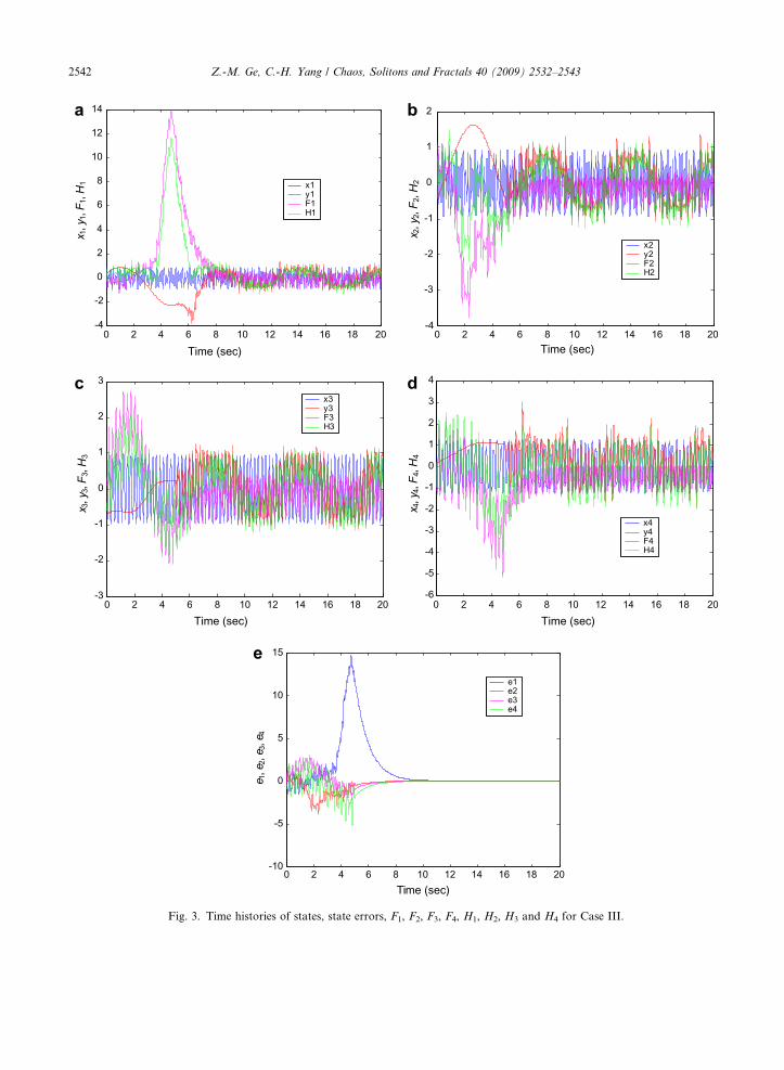
which is negative definite. The Lyapunov asymptotical stability theorem is satisfied. Cubic time delay symplectic syn-chronization of the Quantum-CNN system and the Rossler system is achieved. The numerical results are shown inFig. 3. After 5 s, the motion trajectories enter a chaotic attractor.
0 2 4 6 8 10 12 14 16 18 20-4
-2
0
2
4
6
8
10
12
14
x1y1F1H1
x 1,y
1,F 1
,H1
0 2 4 6 8 10 12 14 16 18 20-6
-5
-4
-3
-2
-1
0
1
2
3
4
x4y4F4H4
0 2 4 6 8 10 12 14 16 18 20-10
-5
0
5
10
15
e1e2e3e4
e 1,e
2,e 3
,e4
Time (sec)
0 2 4 6 8 10 12 14 16 18 20-4
-3
-2
-1
0
1
2
x2y2F2H2
x 2,y
2,F 2
,H2
0 2 4 6 8 10 12 14 16 18 20-3
-2
-1
0
1
2
3
x3y3F3H3
x 3,y
3,F 3
,H3
x 4,y
4,F 4
,H4
Time (sec) Time (sec)
Time (sec) Time (sec)
a b
c d
e
Fig. 3. Time histories of states, state errors, F1, F2, F3, F4, H1, H2, H3 and H4 for Case III.
2542 Z.-M. Ge, C.-H. Yang / Chaos, Solitons and Fractals 40 (2009) 2532–2543
Z.-M. Ge, C.-H. Yang / Chaos, Solitons and Fractals 40 (2009) 2532–2543 2543
4. Conclusions
A new symplectic synchronization of a Quantum-CNN chaotic oscillator and a Rossler system is obtained by theLyapunov asymptotical stability theorem. Two different chaotic dynamical systems, the Quantum-CNN system andthe Rossler system, are in symplectic synchronization for three cases: the cubic symplectic synchronization, the timedelay symplectic synchronization and the cubic time delay symplectic synchronization. Symplectic synchronizationof chaotic systems can be used to increase the security of secret communication.
Acknowledgement
This research was supported by the National Science Council, Republic of China, under Grant Number 96-2221-E-009-144-MY3.
References
[1] Ge Z-M, Yang C-H. The generalized synchronization of a Quantum-CNN chaotic oscillator with different order systems. Chaos,Solitons & Fractals 2008;35:980–90.
[2] Ge Z-M, Yang C-H. Synchronization of complex chaotic systems in series expansion form. Chaos, Solitons & Fractals2007;34:1649–58.
[3] Pecora L-M, Carroll T-L. Synchronization in chaotic system. Phys Rev Lett 1990;64:821–4.[4] Ge Zheng-Ming, Leu Wei-Ying. Anti-control of chaos of two-degrees-of-freedom louderspeaker system and chaos synchroni-
zation of different order systems. Chaos, Solitons & Fractals 2004;20:503–21.[5] Femat R, Ramirez J-A, Anaya G-F. Adaptive synchronization of high-order chaotic systems: a feedback with low-order
parameterization. Physica D 2000;139:231–46.[6] Ge Z-M, Chang C-M. Chaos synchronization and parameters identification of single time scale brushless DC motors. Chaos,
Solitons & Fractals 2004;20:883–903.[7] Femat R, Perales G-S. On the chaos synchronization phenomenon. Phys Lett A 1999;262:50–60.[8] Ge Z-M, Yang C-H. Pragmatical generalized synchronization of chaotic systems with uncertain parameters by adaptive control.
Physica D: Nonlinear Phenomena 2007;231:87–94.[9] Yang S-S, Duan C-K. Generalized synchronization in chaotic systems. Chaos, Solitons & Fractals 1998;9:1703–7.
[10] Krawiecki A, Sukiennicki A. Generalizations of the concept of marginal synchronization of chaos. Chaos, Solitons & Fractals2000;11(9):1445–58.
[11] Ge Z-M, Yang C-H, Chen H-H, Lee S-C. Non-linear dynamics and chaos control of a physical pendulum with vibrating androtation support. J Sound Vib 2001;242(2):247–64.
[12] Chen M-Y, Han Z-Z, Shang Y. General synchronization of Genesio–Tesi system. Int J Bifurcat Chaos 2004;14(1):347–54.[13] Fortuna Luigi, Porto Domenico. Quantum-CNN to generate nanoscale chaotic oscillator. Int J Bifurcat Chaos 2004;14(3):1085–9.[14] Ge Zheng-Ming, Chen Yen-Sheng. Synchronization of unidirectional coupled chaotic systems via partial stability. Chaos, Solitons
& Fractals 2004;21:101–11.[15] Chen S, Lu J. Synchronization of uncertain unified chaotic system via adaptive control. Chaos, Solitons & Fractals
2002;14(4):643–7.[16] Ge Zheng-Ming, Chen Chien-Cheng. Phase synchronization of coupled chaotic multiple time scales systems. Chaos, Solitons &
Fractals 2004;20:639–47.


![Synchronization of Two Fractional-Order Chaotic Systems ...downloads.hindawi.com/journals/jcse/2017/9562818.pdf · in [34, 35], and, furthermore, for fractional-order chaotic systems,](https://img.pdfslide.us/doc/110x75/5f8d11c07c3bc0232b547316/synchronization-of-two-fractional-order-chaotic-systems-in-34-35-and-furthermore.jpg)