Embed Size (px)
Citation preview
( n ./
Symplectic Methods Applied to the Lotka-Volterra System
Melanie Beck
Department of Mathematics and Statistics,
McGill University, Montreal
Quebec, Canada
June, 2003
A thesis submitted to the Faculty of Graduate Studies and Research
in partial fulfillment of the requirements of the degree of
Master of Science
Copyright © Melanie Beck, 2003 % '.::•<:
) i

Abstract
We analyse the preservation of physical properties of numerical approximations to
solutions of the Lotka-Volterra system: its positivity and the conservation of the
Hamiltonian. We focus on two numerical methods : the symplectic Euler method and
an explicit variant of it. We first state under which conditions they are symplectic and
we prove they are both Poisson integrators for the Lotka-Volterra system. Then, we
study under which conditions they stay positive. For the symplectic Euler method,
we derive a simple condition under which the numerical approximation always stays
positive. For the explicit variant, there is no such simple condition. Using properties
of Poisson integrators and backward error analysis, we prove that for initial conditions
in a given set in the positive quadrant, there exists a bound on the step size, such that
numerical approximations with step sizes smaller than the bound stay positive over
exponentially long time intervals. We also show how this bound can be estimated.
We illustrate all our results by numerical experiments.

ii Abstract
I l l
Resume
Nous analysons la preservation des proprietes physiques d'approximations numeriques
des solutions du systeme Lotka-Volterra : sa positivite et la conservation du Hamil-
tonien. Nous nous concentrons sur deux methodes : la methode d'Euler symplec-
tique et une variante explicite de celle-ci. Nous enongons d'abord sous quelles con
ditions ces methodes sont symplectiques et nous prouvons qu'elles sont toutes deux
des integrateurs de Poisson pour le systeme Lotka-Volterra. Puis nous etudions sous
quelles conditions elles sont positives. Pour la methode d'Euler symplectique, nous
obtenons une condition simple sous laquelle l'approximation numerique reste toujous
positive. Pour la variante explicite, il n'y a pas de condition aussi simple. En utilisant
les propriets des integrateurs de Poisson et l'analyse implicite de l'erreur ("backward
error analysis"), nous prouvons que pour des conditions initiales appartenant a un
ensemble donne dans le quadrant positif, il existe une borne sur le pas de temps,
telle que les approximations numeriques avec un pas de temps plus petit que cette
borne restent positives sur des intervalles exponentiellement longs. Nous montrons
egalement comment cette borne peut etre estimee. Nous illustrons tous nos resultats
pas des experiences numeriques.

IV Resume
Acknowledgments
Je voudrais tout d'abord remercier mon superviseur, Martin J. Gander, pour son
aide, son soutien, ses encouragements et ses suggestions ; le temps qu'il consacre a
ses etudiants est impressionnant. Sans lui, je n'aurais jamais commence de maitrise,
et j'aurais encore moins termine cette maitrise. He is such an excellent supervisor!
J'aimerais egalement remercier Ernst Hairer et Gerhard Wanner pour m'avoir
invitee a participer au seminaire d'analyse numerique de l'Universite de Geneve, ainsi
que pour les discussions concernant mon projet de recherche et les idees qu'ils m'ont
apportees. Merci aussi pour leur ouvrage [5] si complet.
Merci a Olivier Dubois et Charles Fortin pour avoir relu ma these et suggere des
ameliorations.
I would like to thank the professors of applied mathematics in the department, in
particular Nilima Nigam, Paul Tupper, Georg Schmidt, Tony Humphries and Peter
Bartello, for their efforts in making the department more and more friendly, pleasant
and enjoyable for studying.
I also want to thank the Department of Mathematics and Statistics, l'lnstitut
des Sciences Mathematiques and the Faculty of Graduate Studies, for their financial
support.
Finalement je remercie ma famille et mes amis des deux cotes de l'Atlantique,
grace a qui ma vie d'etudiante est si agreable.

vi Acknowledgments
V l l
Table of Contents
Abstract i
Resume iii
Acknowledgments v
Introduction 1
1 Preliminaries 5
1.1 Historical Bibliography 5
1.2 The Lotka-Volterra System 7
2 Different Methods Applied to the Lotka-Volterra System 13
2.1 Forward Euler 13
2.2 Backward Euler 14
2.3 Symplectic Euler 17
2.4 Explicit Variant of symplectic Euler 19
3 Symplectic Methods and Poisson Integrators 23
3.1 Symplecticity 23
3.2 Poisson Integrators 25
3.3 Symplectic Euler 28
viii TABLE OF CONTENTS
3.4 Explicit Variant of Symplectic Euler 34
4 Backward Error Analysis 41
4.1 Properties of Symplectic Methods and Poisson Integrators 41
4.2 The Symplectic Euler Method 44
4.3 The Structure of the Numerical Hamiltonian 49
4.4 The Explicit Variant of the Symplectic Euler Method 62
4.5 Structure of the Numerical Hamiltonian 65
4.6 Concluding Remarks 68
5 Exploitation of the Numerical Hamiltonian 71
5.1 Estimation of the Numerical Solution 72
5.2 Estimation of the Coefficients of the Modified Equation 73
5.3 Estimation of the Local Error 78
5.4 Estimates of the Variation of the Hamiltonian 81
5.5 Application 84
5.6 Example 87
Conclusion 89
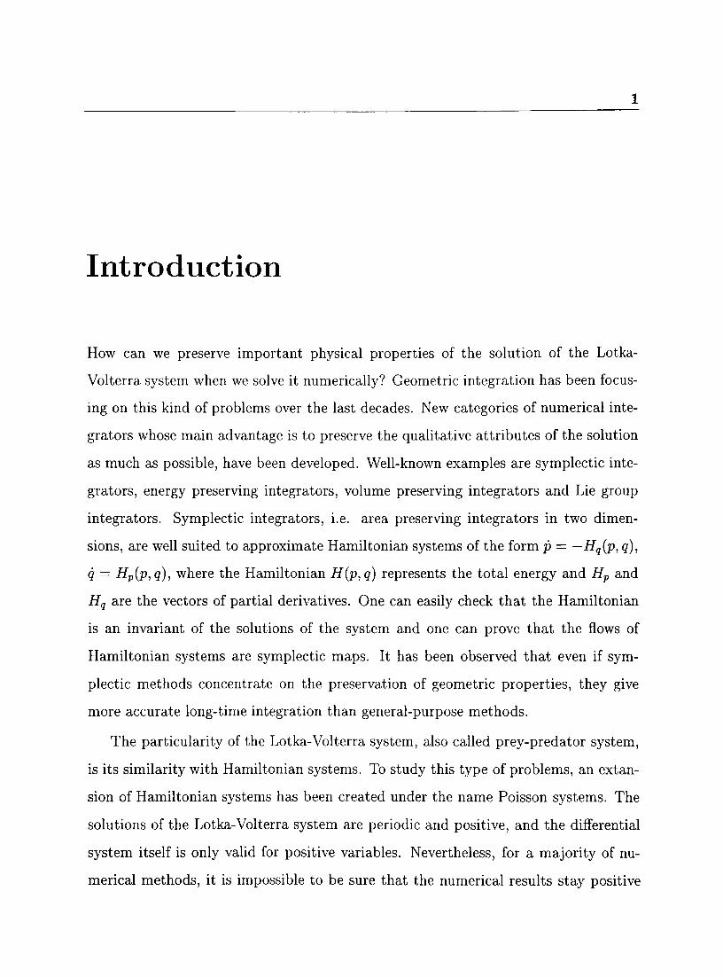
Introduction
How can we preserve important physical properties of the solution of the Lotka-
Volterra system when we solve it numerically? Geometric integration has been focus
ing on this kind of problems over the last decades. New categories of numerical inte
grators whose main advantage is to preserve the qualitative attributes of the solution
as much as possible, have been developed. Well-known examples are symplectic inte
grators, energy preserving integrators, volume preserving integrators and Lie group
integrators. Symplectic integrators, i.e. area preserving integrators in two dimen
sions, are well suited to approximate Hamiltonian systems of the form p = —Hq(p, q),
q = Hp(p,q), where the Hamiltonian H(p,q) represents the total energy and Hp and
Hq are the vectors of partial derivatives. One can easily check that the Hamiltonian
is an invariant of the solutions of the system and one can prove that the flows of
Hamiltonian systems are symplectic maps. It has been observed that even if sym
plectic methods concentrate on the preservation of geometric properties, they give
more accurate long-time integration than general-purpose methods.
The particularity of the Lotka-Volterra system, also called prey-predator system,
is its similarity with Hamiltonian systems. To study this type of problems, an extan-
sion of Hamiltonian systems has been created under the name Poisson systems. The
solutions of the Lotka-Volterra system are periodic and positive, and the differential
system itself is only valid for positive variables. Nevertheless, for a majority of nu
merical methods, it is impossible to be sure that the numerical results stay positive
Introduction
and consequently we can not expect a good long-time approximation. It is therefore
important to study the possibilities offered by specific " Poisson integrators".
This thesis' focus is a specific method, the symplectic Euler method, and an
explicit variant of it. Both methods are Poisson integrators for the Lotka-Volterra
system and our interest lies in the preservation of the positivity. For the symplectic
Euler method, very simple arguments yield the desired result: if the step-size is chosen
smaller than a bound determined by the problem (namely, the minimum of the inverse
of the equilibrium point's coordinates), the numerical solution stays positive for all
time. In contrast, for an explicit variant of this method, much more work is needed
and important properties of Poisson integrators have to be used to show a similar
result. In particular, backward error analysis is the key tool. The final result shows
how to compute, for given initial conditions, a bound h* such that every numerical
solution obtained with a step-size smaller than h*, is really close to the exact solution
and remains positive for exponentially long time intervals.
In the first chapter, after a short historical bibliography on the symplectic Euler
method, we present the Lotka-Volterra system and its properties.
The second chapter contains illustrations of some classical methods applied to
the Lotka-Volterra system together with the advantages and disadvantages of these
methods.
We introduce, in the third chapter, the notions of symplecticity and of Poisson
integrators, and we also study in more details two methods : the symplectic Euler
method and an explicit variant of it. We study their symplecticity, whether or not
they are Poisson integrators for the Lotka-Volterra system and finally we study their
positivity (when applied to the Lotka-Volterra system).
The fourth chapter is devoted to the backward error analysis; after defining this
concept, we state some properties of symplectic methods and Poisson integrators and
compute the first terms of the numerical Hamiltonians of the symplectic Euler method
and its explicit variant. We also study the structure of these numerical Hamiltonians.
The fifth and last chapter exploits backward error analysis. We focus on the
explicit variant of the symplectic Euler method and prove the important theorem
concerning the choice of the step-size ensuring the positivity of the numerical result
for exponentially long time intervals.

Introduction
Chapter 1
Preliminaries
1.1 Historical Bibliography
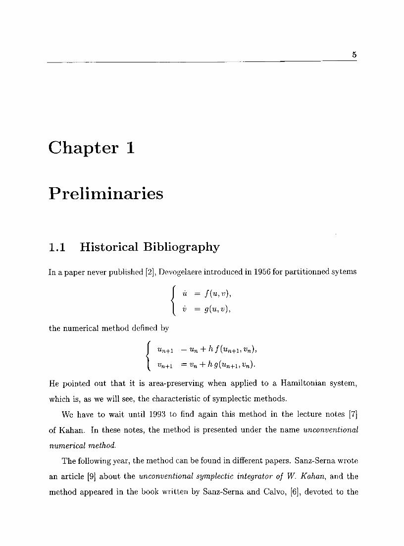
In a paper never published [2], Devogelaere introduced in 1956 for partitionned sytems
u = f(u,v),
v = g{u,v),
the numerical method defined by
un+x =un + hf(un+i,vn),
vn+i =vn + hg(un+1,vn).
He pointed out that it is area-preserving when applied to a Hamiltonian system,
which is, as we will see, the characteristic of symplectic methods.
We have to wait until 1993 to find again this method in the lecture notes [7]
of Kahan. In these notes, the method is presented under the name unconventional
numerical method.
The following year, the method can be found in different papers. Sanz-Serna wrote
an article [9] about the unconventional symplectic integrator of W. Kahan, and the
method appeared in the book written by Sanz-Serna and Calvo, [6], devoted to the
6 Preliminaries
numerical approximation of Hamiltonian problems. However in this text the method
is not given any specific name; it is presented as the first order symplectic Runge-
Kutta method. In the mean time, Hairer introduced the method in [4] motivated by
the backward error analysis and called it the symplectic Euler method. In [3], Gander
studied particularly the Lotka-Volterra equation, and in order to have an explicit
method, he defined the symplectic Euler method as
un+i =un + hf(un,vn),
vn+i =vn + hg(un+i,vn).
Later, in 2000, Meyer-Spasche and Gander studied several numerical integrators
preserving physical properties in [8]. They continued studying the explicit variant of
the symplectic Euler method and applied it to Hamiltonian problems with separable
Hamiltonian and to the Lotka-Volterra system. The same year, two physicists, Stur
geon and Laird used the symplectic Euler method in [10] to define the Stormer-Verlet
scheme, a composition of the symplectic Euler method and its adjoint.
The study of the symplectic Euler method continued in a few papers written
in 2002. In a chapter of his thesis [11], Tupper explored the results obtained by
different numerical methods applied to a Hamiltonian system on long time intervals
and using large step sizes. He illustrated the excellent performance of the symplectic
Euler method and the mediocrity of one-step-and-project methods in the context of
long-time statistics. In Norway, Berland studied in his diploma thesis [1] numerical
methods, including the symplectic Euler method, by the means of Lie group theory.
Finally in that same year, Hairer, Lubich and Wanner published the most complete
book written up to date on geometric numerical integration, [5]. Most of the results
observed about the symplectic Euler method, and even more, can be found in this
reference.
1.2 The Lotka-Volterra System 7
1.2 The Lotka-Volterra System
This thesis mainly focuses on the numerical approximation of the Lotka-Volterra
system
u = u(b-v),
ii = v (u — a),
which models the evolution of two animal species. Here u(t) is the number of prey
and v(t) the number of predators. Actually, u and v are continuous variables since
we consider densities and not numbers of individual. The constants a and b depend
on the two animal species considered, b is the growing rate of preys, when there is
no predator, and a represents the tendance of extinction of the predators when there
is no prey. The term uv is related to the decreasing rate of preys due to predators
in the first equation and to the rate of variation of predators corresponding to the
quantity of available food in the second equation.
The Lotka-Volterra system is interesting due to its geometric property : every
solution of (1.1) lies on a closed curve (actually one can even show that it is periodic).
If we divide the two equations of the Lotka-Volterra system (1.1), we obtain
ii u(b — v) v v(u — a) '
which becomes, after separation of variables,
u — a . b — v . u v = 0.
u v
Integrating this equality we obtain an invariant of the system,
H(u,v) = u — a\nu + v — b\nv. (1.2)
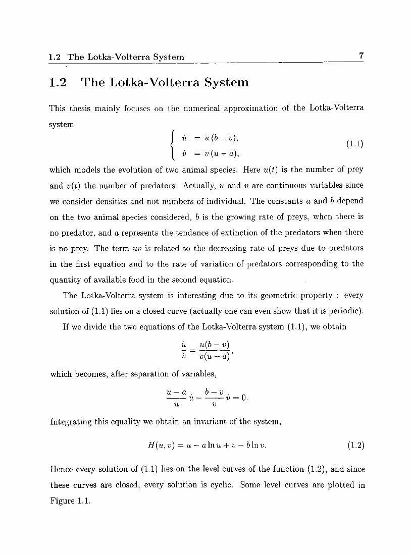
Hence every solution of (1.1) lies on the level curves of the function (1.2), and since
these curves are closed, every solution is cyclic. Some level curves are plotted in
Figure 1.1.
8 Preliminaries
Figure 1.1: Some level curves of the Hamiltonian of the Lotka-Volterra system, from
H = 2.1 to H = 3.7.
If H is defined by (1.2), the Lotka-Volterra system can be written as
u = —uvHv(u,v),
v = uv Hu(u, v),
where Hu and Hv denote the partial derivatives of H with respect to u and v. In other
words, the system is not Hamiltonian but it is a non-canonical Hamiltonian system,
or more generally a Poisson system (a more precise definition is given in Chapter 3).
This explains why thereafter we call H the Hamiltonian of the system.
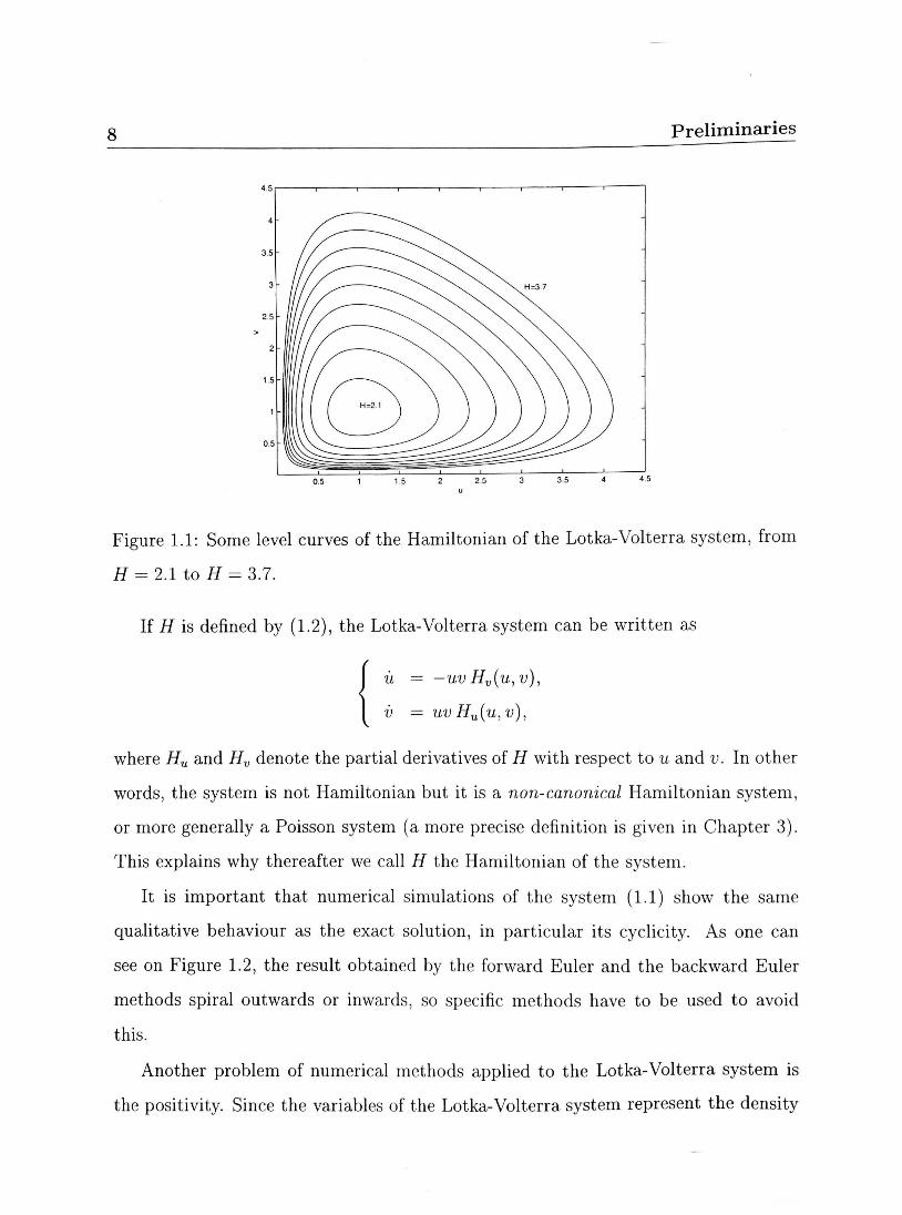
It is important that numerical simulations of the system (1.1) show the same
qualitative behaviour as the exact solution, in particular its cyclicity. As one can
see on Figure 1.2, the result obtained by the forward Euler and the backward Euler
methods spiral outwards or inwards, so specific methods have to be used to avoid
this.
Another problem of numerical methods applied to the Lotka-Volterra system is
the positivity. Since the variables of the Lotka-Volterra system represent the density
1.2 The Lotka-Volterra System 9
0 Forward Euler method + Backward Euler method
I I Trajectory ol the exact solution
Figure 1.2: Illustration of the forward Euler and the backward Euler methods, with
u0 = 0.5, VQ = 0.5, a = b = 1 and h = 0.1.
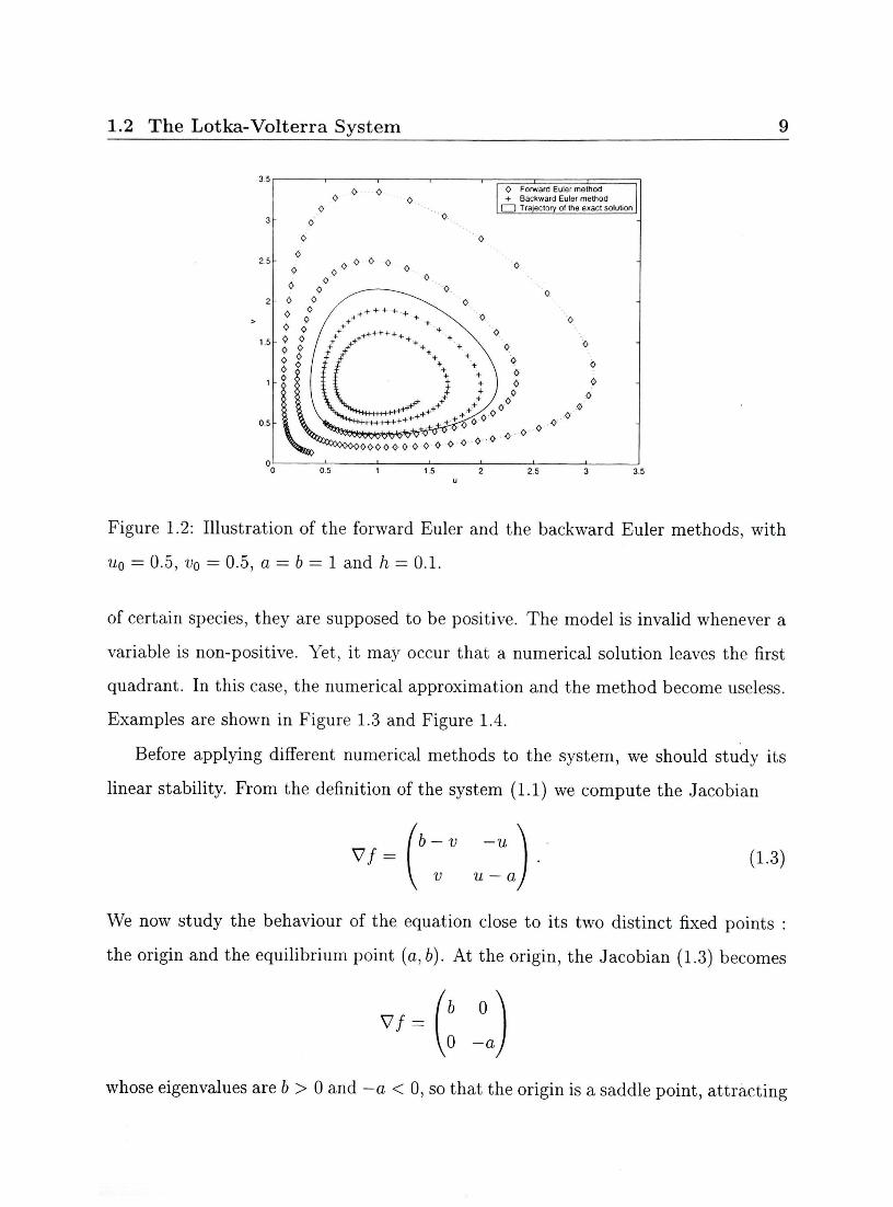
of certain species, they are supposed to be positive. The model is invalid whenever a
variable is non-positive. Yet, it may occur that a numerical solution leaves the first
quadrant. In this case, the numerical approximation and the method become useless.
Examples are shown in Figure 1.3 and Figure 1.4.
Before applying different numerical methods to the system, we should study its
linear stability. From the definition of the system (1.1) we compute the Jacobian
V/ = b — v —u
;i.3) v u — a
We now study the behaviour of the equation close to its two distinct fixed points :
the origin and the equilibrium point (a, b). At the origin, the Jacobian (1.3) becomes
V/ = b 0
0 -a
whose eigenvalues are b > 0 and - a < 0, so that the origin is a saddle point, attracting
10 Preliminaries
5 -
+ ,
+.
1
+ • - + .
+
1
'•'+
r
' + • . . .
.. +
+
+
10 12 14
Figure 1.3: Illustration of the forward Euler method when the solution leaves the first
quadrant. UQ = 0.5, VQ = 0.5 and h = 0.3.
along v and repulsive along u. At the equilibrium point the Jabobian becomes
V/ = 0 -a
b 0
and its eigenvalues are ±ivab. Hence the equilibrium point is hyperbolic and the
solution is rotating around it. This analysis is confirmed by the shape of the level
curves given in Figure 1.1.
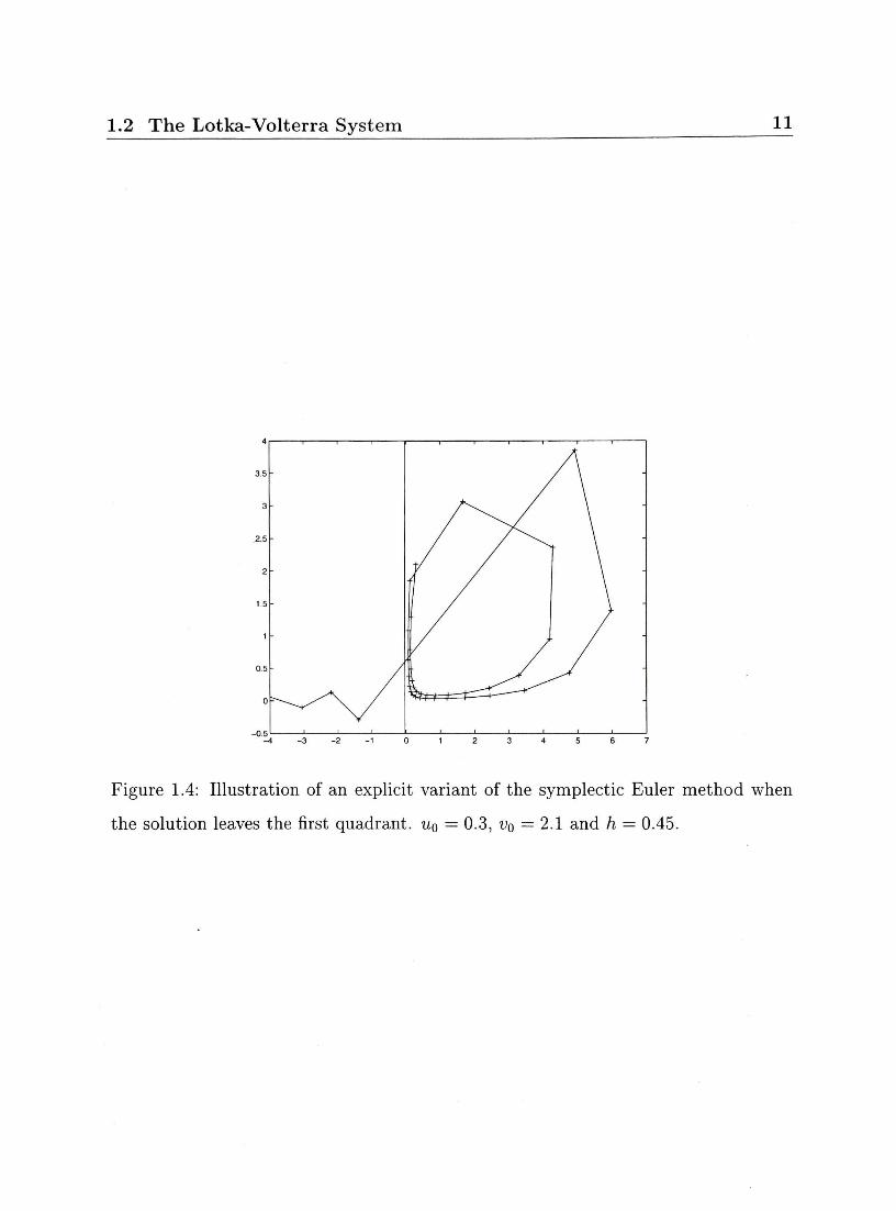
1.2 The Lotka-Volterra System 11
Figure 1.4: Illustration of an explicit variant of the symplectic Euler method when
the solution leaves the first quadrant. uQ = 0.3, VQ = 2.1 and h — 0.45.

1 o Preliminaries
13
Chapter 2
Different Methods Applied to the
Lotka-Volterra System
As an illustration, we apply classical numerical methods to the Lotka-Volterra system
and observe their properties. To simplify the computation of implicit methods, we
consider the system when a and b are both equal to one:
ii = u{l-v) = f(u,v),
v = v (u — 1) = g(u,v).
2.1 Forward Euler
The forward Euler method, given by
Un+l =Un + hf{un,Vn),
vn+i =vn + hg{un,vn),
is easy to implement because it is an explicit method. When we apply it to the
Lotka-Volterra system, un+i and vn+i are given by
un+i = un + hun{\ - vn),
Vn+l = Vn + hvn (Un - 1).
14 Different Methods Applied to the Lotka-Volterra System
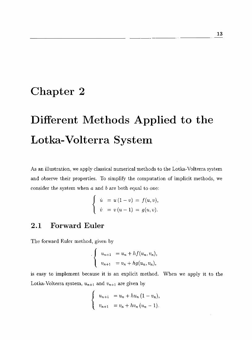
Figure 2.1: Illustration of the performance of the forward Euler method applied to
the Lotka-Volterra system, with u0 = 0.5, v0 = 0.5 and h = 0.1.
Figure 2.1 shows the numerical solution obtained with the forward Euler method
for h = 0.1. We observe that it spirals outwards whereas the exact solution should
lie on a closed curve (the solid line on the figure).
2.2 Backward Euler
The backward Euler method is an implicit method given by
un+l =un + hf(un+i,vn+i),
Vn+i = vn + hg(un+i, vn+i);
yet, for the Lotka-Volterra system, one can explicitely advance it because of the simple
form of / and g: to express un+1 and un+1 as functions of un and vn, we first derive
from the first equation of the method
Un+l u.
1 - h{\ -vn+1)
2.2 Backward Euler 15
Substituting this definition of wn+1 into the second equation of the method,
vn+i = vn + hvn+l(un+i - 1),
we obtain an equation of second order in vn+i, whose solutions are
h Ur, ± \j{\ -h-un- vn)2 + 4(1 + h)vn(^ - 1)
2(1+ /i) V
Now we have to choose one of these two solutions. As h goes to zero, the numerical
result should converge to the exact solution, in particular vn+\ should stay bounded.
Since the terms of \/h blow up as h goes to zero, the correct root is the one with
the positive sign, so that the terms (1/h — h — un — vn) balance themselves. One can
indeed check, for example using Maple, that the first term of the expansion of the
solution with the negative sign is —1/h whereas the first term of the expansion of the
solution with the positive sign is vn.
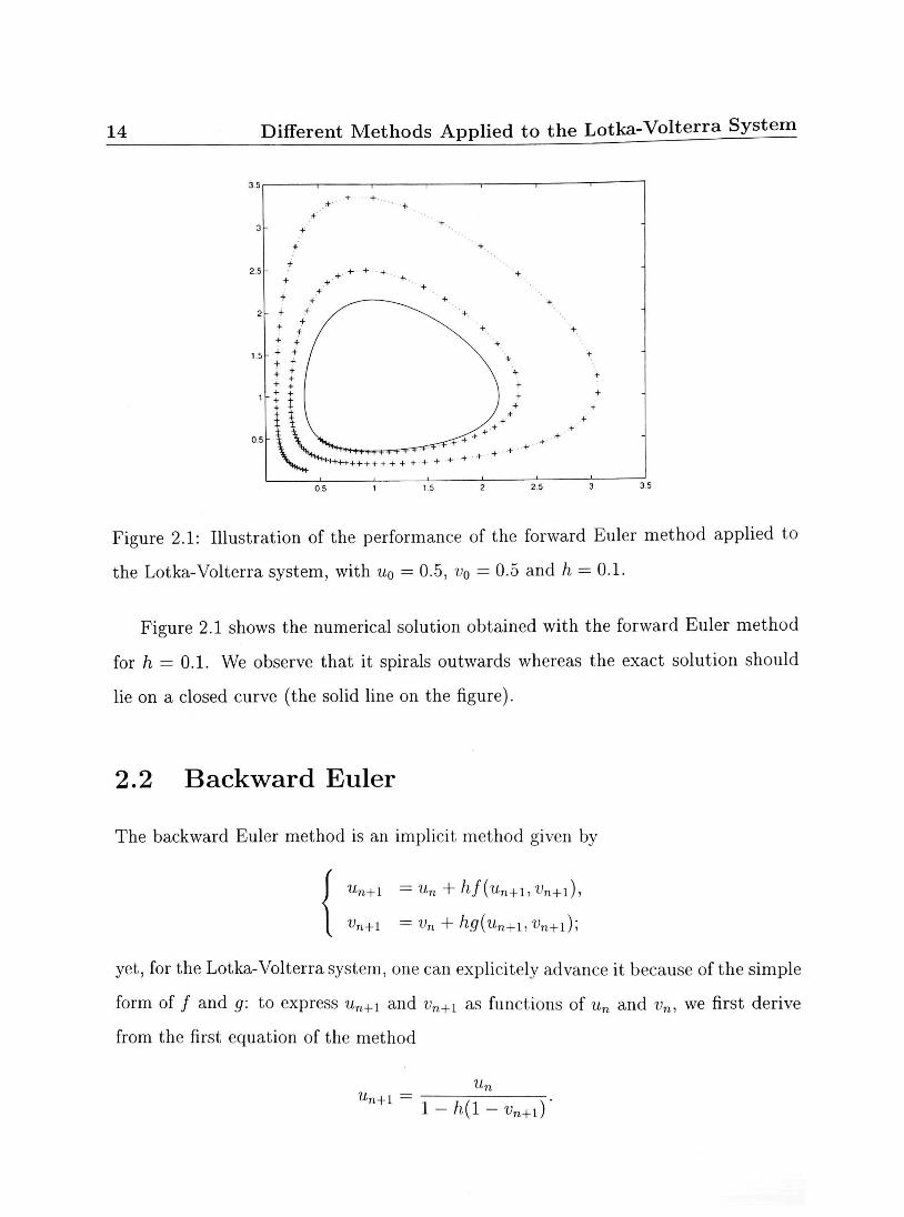
Figure 2.2: Illustration of the performance of the backward Euler method applied to
the Lotka-Volterra system when we use the root with the negative sign for vn+i, with
UQ = 0.5, VQ = 0.5, and h = 0.1.
16 Different Methods Applied to the Lotka-Volterra System
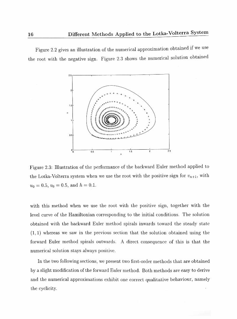
Figure 2.2 gives an illustration of the numerical approximation obtained if we use
the root with the negative sign. Figure 2.3 shows the numerical solution obtained
Figure 2.3: Illustration of the performance of the backward Euler method applied to
the Lotka-Volterra system when we use the root with the positive sign for vn+i, with
u0 = 0.5, v0 = 0.5, and h = 0.1.
with this method when we use the root with the positive sign, together with the
level curve of the Hamiltonian corresponding to the initial conditions. The solution
obtained with the backward Euler method spirals inwards toward the steady state
(1,1) whereas we saw in the previous section that the solution obtained using the
forward Euler method spirals outwards. A direct consequence of this is that the
numerical solution stays always positive.
In the two following sections, we present two first-order methods that are obtained
by a slight modification of the forward Euler method. Both methods are easy to derive
and the numerical approximations exhibit one correct qualitative behaviour, namely
the cyclicity.
2.3 Symplectic Euler 17
2.3 Symplectic Euler
The symplectic Euler method is defined in [4] by
un + i =un + hf(un+l,vn),
Vn+1 =Vn + hg(Un+UVn),
and gives, when applied to the Lotka-Volterra system
un+l =un + hun+1(l-vn),
vn+x =vn + hvn(un+1-l),
(2.1)
that is 11 , — "n
"n+1 — i_h (1—«„)' vn+1 = vn + hvn{un+i - 1).
(2.2)
A
. -i-h -
^
A-
i
+ Symplectic Euler method | 1 Trajectory of the exact solution
\ +
\ + \v V \ +
i •
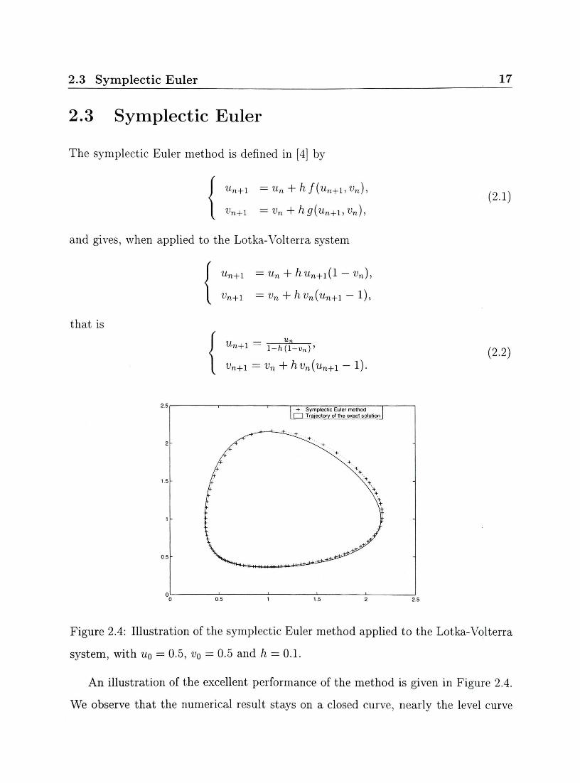
Figure 2.4: Illustration of the symplectic Euler method applied to the Lotka-Volterra
system, with u0 = 0.5, v0 = 0.5 and h = 0.1.
An illustration of the excellent performance of the method is given in Figure 2.4.
We observe that the numerical result stays on a closed curve, nearly the level curve
18 Different Methods Applied to the Lotka-y^Uerra^ys^em
-35 -30 -25 -20 -15 -10
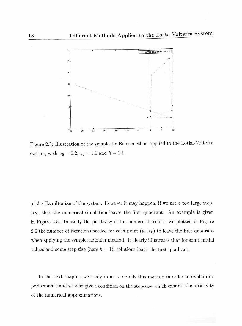
Figure 2.5: Illustration of the symplectic Euler method applied to the Lotka-Volterra
system, with u0 = 0.2, v0 = 1.1 and h = 1.1.
of the Hamiltonian of the system. However it may happen, if we use a too large step-
size, that the numerical simulation leaves the first quadrant. An example is given
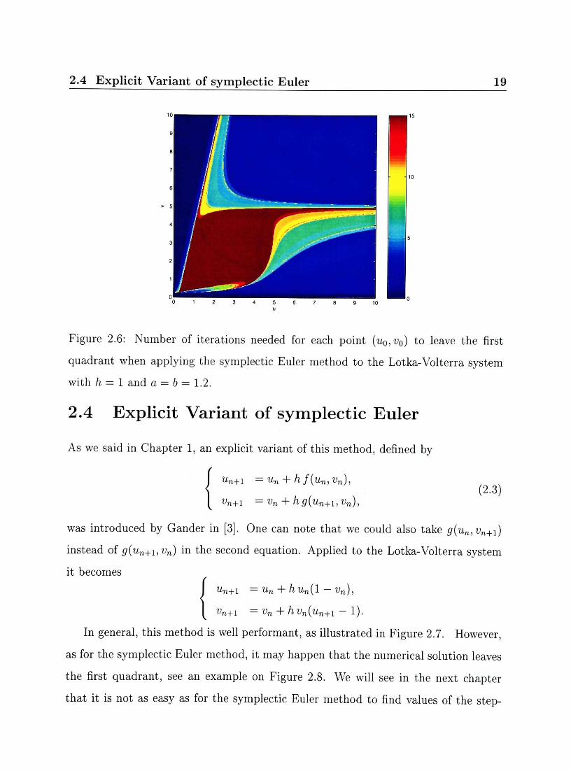
in Figure 2.5. To study the positivity of the numerical results, we plotted in Figure
2.6 the number of iterations needed for each point (uo, v0) to leave the first quadrant
when applying the symplectic Euler method. It clearly illustrates that for some initial
values and some step-size (here h = 1), solutions leave the first quadrant.
In the next chapter, we study in more details this method in order to explain its
performance and we also give a condition on the step-size which ensures the positivity
of the numerical approximations.
2.4 Explicit Variant of symplectic Euler 19
Figure 2.6: Number of iterations needed for each point (u0,v0) to leave the first
quadrant when applying the symplectic Euler method to the Lotka-Volterra system
with h — 1 and a = b = 1.2.
2.4 Explicit Variant of symplectic Euler
As we said in Chapter 1, an explicit variant of this method, defined by
(2.3) un+i =un + hf(un,vn),
vn+\ = vn + hg(un+1,vn),
was introduced by Gander in [3]. One can note that we could also take g{un,vn+i)
instead of g(un+x, vn) in the second equation. Applied to the Lotka-Volterra system
it becomes
Un+1 =Un + hun(l-Vn),
Vn+l =Vn + hvn(un+i-l).
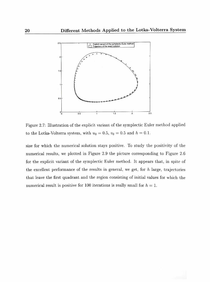
In general, this method is well performant, as illustrated in Figure 2.7. However,
as for the symplectic Euler method, it may happen that the numerical solution leaves
the first quadrant, see an example on Figure 2.8. We will see in the next chapter
that it is not as easy as for the symplectic Euler method to find values of the step-
20 Different Methods Applied to the Lotka-Volterra System
Explicit variant of the symplectic Euler method I Trejectory ol the exact solution
Hi H i •»
Figure 2.7: Illustration of the explicit variant of the symplectic Euler method applied
to the Lotka-Volterra system, with u0 = 0.5, vQ = 0.5 and h = 0.1.
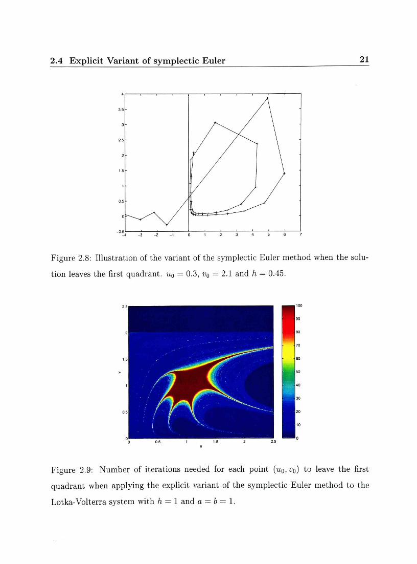
size for which the numerical solution stays positive. To study the positivity of the
numerical results, we plotted in Figure 2.9 the picture corresponding to Figure 2.6
for the explicit variant of the symplectic Euler method. It appears that, in spite of
the excellent performance of the results in general, we get, for h large, trajectories
that leave the first quadrant and the region consisting of initial values for which the
numerical result is positive for 100 iterations is really small for h = 1.
2.4 Explicit Variant of symplectic Euler 21
Figure 2.8: Illustration of the variant of the symplectic Euler method when the solu
tion leaves the first quadrant. uQ = 0.3, VQ = 2.1 and h = 0.45.
Figure 2.9: Number of iterations needed for each point (U0,VQ) to leave the first
quadrant when applying the explicit variant of the symplectic Euler method to the
Lotka-Volterra system with h = 1 and a = b = 1.

22 Different Methods Applied to the Lotka-Volterra System
23
Chapter 3
Symplectic Methods and Poisson
Integrators
In this chapter, after introducing the notions of symplecticity and of Poisson integra
tors, we study in more details the symplectic Euler method and its explicit variant
defined in Section 2.3 and Section 2.4. We study their symplecticity, under which
conditions they are Poisson integrators and if it possible to find for which step-sizes
the numerical solution stays positive.
3.1 Symplecticity
Before defining symplecticity, we need to introduce an important concept in the study
of differential equations: the flow over time t. This map, denoted by cf>t, associates
to any point y0 in the phase space, the value y(t) of the solution with initial value
y(0) = y0. In other words, it is defined by
<i>t{yo) = y{t) if 2/(0) = y0.
24 Symplectic Methods and Poisson Integrators
As proved in [8], an interesting property of Hamiltonian systems of the form
<7 = ^ ( P > * ) ,
W^>^> (3.1) I
dp
where H(p, q) is the Hamiltonian, is, when p and q are scalars, area preservation.
Transformations that have this property are called symplectic. A generalization to
higher dimensions of the definition of symplecticity is given in [5]:
Definition 3.1. A differentiable map g : U ->• R2d (where U C R2d is an open set) is
called symplectic, if the Jacobian matrix g'(p, q) is everywhere symplectic:
g'(p,q)TJ g'(p,q) = f
where
\ - I 0
This definition allows us to consider systems of any dimensions: the oriented
area of two-dimensional parallelograms P lying in R2, is replaced by the sum of
the oriented areas of the projections of 2d-dimensional parallelograms P onto the
coordinate planes (pi,qi). Symplecticity is a characteristic of Hamiltonian systems,
more precisely the flows of Hamiltonian systems are symplectic maps. This motivates
the following definition of symplecticity of numerical methods.
Definition 3.2. A numerical method is called symplectic, if the one-step map t/i =
$h(yo) is symplectic whenever the method is applied to a smooth Hamiltonian system.
This means that a numerical method is symplectic if and only if
fd(P+l,qn+i)\T j (d(P+1,q ,)\ = j
\ d(pn,qn) J \ d{pn,qn) J
whenever it is applied to the smooth Hamiltonian system (3.1).
3.2 Poisson Integrators 25
To check symplecticity in the case where p and q are scalars, there exists a simpler
way (see for example [6]): if we consider a C^transformation
defined on a set D, according to the standard rule for changing variables in an integral,
ip preserves area and orientation if and only if the Jacobian determinant is identically
one, that is
w , . _ du* dv* du* dv* „ .„ „x
V u . v e D , — — - — _ = l. (3.3) ou dv dv du
This condition is equivalent to the matrix equation (3.2), in the case where p and q are scalars. Now we consider the differentials
, „ du* du* J , , „ dv* , dv* , du = -r—du + ——dv and dv = -^—du + -r—dv
du dv du dv
and we compute their wedge product (also called exterior product), du A dv. This
product is bilinear and skew-symmetric (i.e. du A du = dv A dv = 0 and du A dv =
—du A du), so we get
, , , „ du*dv* , du* dv* , , 5u* 5v* J , 5u* 5w* , du Adv = -r— -r— du Adu + — — — du A du + -^— -^— dv A du + ——— d v . A d v
du du du dv dv du dv dv _ (du^dy^_ duf_dy^\
\ du dv dv du J
Consequently, according to the characterization of symplecticity (3.3), the method is
symplectic if and only if
dun+i A dvn+i = dun A dvn for all (un, vn).
3.2 Poisson Integrators
As we said in Chapter 1, the Lotka-Volterra system is not Hamiltonian but its struc
ture is similar to a Hamiltonian system. In fact, the right hand sides are only multi
plied by uv in addition. In other words, we can write the Lotka-Volterra system as
2(3 Symplectic Methods and Poisson Integrators
y = B(y)VH(y), (3-4)
where y = (u,v), H(y) = u - a\nu + v - b\nv and
( 0 -uv \ ln cx
(3-5) uv 0 ]
The generalization (3.4) of a Hamiltonian system is called a Poisson system.
Definition 3.3. If a matrix B(y) is skew-symmetric and satisfies
£ (^kk(y) + ^ K i v ) + ^ M v ) ) = 0, for all UX (3.6)
then the formula
l=1 v oyi oyi dyi
W G } W = t ^ M ^ (3.7)
is said to represent a general Poisson bracket. The corresponding differential system
(3.4) is a Poisson system. We continue to call H the Hamiltonian.
Since the Lotka-Volterra system can be written in the form (3.4), where B{y),
defined in (3.5), is skew-symmetric and satisfies (3.6), it is a Poisson system. To
study such systems, the notion of Poisson maps is essential.
Definition 3.4. A transformation ip : U -> Rn (where U is an open set in Rn) is
called a Poisson map with respect to the Poisson bracket (3.7), if its Jacobian matrix
satisfies
<p'(y)B(y)<p'(y)T = B(<p(y)).
We observe, of course, a similarity with symplectic maps. The following theorem,
whose proof can be found in [5], explains the relation between Poisson systems and
Poisson maps.
3.2 Poisson Integrators 27
Theorem 3.5. If B(y) is the structure matrix of a Poisson bracket, the flow f>t{y)
of the differential system
y = B{y)VH{y)
is a Poisson map.
It would of course be interesting to choose numerical methods which exhibit the
same characteristics as the flow y>t(y) when solving this kind of problems. This
motivates the introduction of the notion of Poisson integrators, but before stating its
definition we need to introduce the Casimir functions.
Theorem 3.6. Suppose that the matrix B(y) defines a Poisson bracket and is of
constant rank n — q — 2m in a neighbourhood of yo (zW1. Then, there exist functions
Pi{y),...,Pm{y), Qi(y),---,Qm{y), andCi{y),...,Cq{y) satisfying
{Pt,P3} = 0 {P«Qj\ = -6ij {Pi,G} = 0
{Qi,Pj} = Stj {Qi,Qj} = 0 {Qi,G} = 0
{Ck,Pj\ = 0 {C*,Q,} = 0 {C*,Ci} = 0
on a neighbourhood ofyo. The gradients of P{,Qj,Ck are linearly independent, so that
y •-»• (Pi{y),Qi(y),Ck(y)) constitutes a local change of coordinates to canonical form.
The proof of this theorem can be found in [5]. The functions Ck are called Casimirs
and the flow (pt{y) of a Poisson system respects them in the sense that Ci(<pt(y)) —
Const. This motivates the following definition.
Definition 3.7. A numerical method y\ = $h(yo) is a Poisson integrator for the
structure matrix B(y), if the transformation u0 i-> y\ respects the Casimirs and if it
is a Poisson map whenever the method is applied to the corresponding differential
system (3.4).
In the case of the Lotka-Volterra system, the matrix B(y) is of rank 2 for all
y = (u,v) € D = {(u,v) : u > 0, v > 0}, so there is no Casimir function (since
28 Symplectic Methods and Poissonjntegrators
q = 0) and a numerical method is a Poisson integrator for B(y) if and only if it is a
Poisson map whenever applied to the Poisson system (3.4), in other words we need
it to satisfy
(d(un+l,Vn+1)\T I 0 ~UnVn\ fd(un+l,Vn+l)\ = / 0 -Un+lVn+l
V d{un,vn) ) \UnVn 0 I V d(un,vn) J U n + 1 u n + i 0 X ' (3.8)
The most interesting property of Poisson integrators is related to the backward
error analysis which is the topic of the next chapter.
3.3 Symplectic Euler
The main characteristic of the symplectic Euler method (2.1) is its symplecticity.
Theorem 3.8. If the matrix I + hHpq, where I is the identity and Hpq is the matrix
of partial derivatives evaluated at (Pn+\,qn), is invertible, then the symplectic Euler
method (2.1) is symplectic. The condition is always satisfied for h small enough.
Proof. We have to prove that this method is symplectic in the sense of the definition
given in [5], that is we have to prove the symplecticity characterization (3.2).
Applying the symplectic Euler method to a smooth Hamiltonian system gives
Pn+i =Pn~ h^{pn+uqn),
qn+i =qn + h^{pn+l,qn),
and differentiating these expressions with respect to pn and qn, we obtain
dP"+i — J _ h^XL(n , n ^ P n + 1 dpn
x ndpdq\lJn+l,Hn) dpn ,
dPi+i - -h^LLfn , / , U h^JLfn n ^ P " + > dqn ~ ndqdq\Pn+li(ln) ,l dpdq \Pn+l, 9n) gqn ,
d1n+x _ i d2H l \dpn + i
dpn ndpdpyPn + l ^ n l dpn '
{ ^ = ^hg-p(Pn+uqn) + h0-p(Pn+uqn)d-^.
3.3 Symplectic Euler 29
This system can be written as a matrix equation
J + AHJ ° | [ ^ ^ l . (3.9)
where the matrices Hqp,Hpp,Hqq of partial derivatives are evaluated at (pn+i,qn)-
To simplify notations, we define A := I + hHqp. Assuming that the first matrix in
equation (3.9) is invertible, that is det A / 0, we can compute the matrix of derivatives
d$h: =
where
AT 0 \ l _ ( A~T 0
-hHpp I j \hHppA-T I
We can now compute the matrix product
'd{pn+i,qn+i)\T j (d{pn+uqn+iY
l~T 0\ II -hHqq
hHppA~T I
and the symplecticity of the method is proved.
•
Since the Lotka-Volterra system is a Poisson system, we can check whether or not
the symplectic Euler method is a Poisson integrator for this system.
30 Symplectic Methods and Poisson Integrators
Theorem 3.9. The symplectic Euler method (2.1) is a Poisson integrator for Poisson
systems with B(y) defined in (3.5) and any separable Hamiltonian H such that 1 +
hvn(Hv - un+lHuv) is not zero. This condition is always satisfied if h is chosen small
enough.
Proof. We need to prove that the condition (3.8) is satisfied whenever we apply the
symplectic Euler method to a system of the form
u = —uvHv(u,v),
v = uvHu(u, v).
We differentiate un+i = un - hun+ivnHv(un+1,vn),
vn+i = vn + hun+iVnHu(un+i,vn)
with respect to (un, vn) and write the results as a matrix equation
\ + hvn(Hv - un+1Huv) o \ / ^ ± i *£±i \ = A -hun+1(Hv + vnHvv)
-hvn(Hu + un+lHuu) 1) \ ^ d-^j \0 l + hun+i{Hu + vnHvu)^
where the matrices HUV,HUU,HVV of partial derivatives are evaluated at (un+i,vn).
Assuming 1 + hvn(Hv — un+iHuv) is not zero, we have
l + te„(tf„-«„+1ff„) <>\ = / i+to„(H.iu,„H,„) o
-hvn(Hu+un,lH„) i) [tiifc::'"^ i and we can compute
( Q -unvn(l+hun+i(Hu+vnHvu))
l+hvn(Hv-un+1Huv) UnVn{l+hun+l{Hu+VnHvu)) r\
l+hvn(Hv-un+iHuv) Therefore the symplectic Euler method is a Poisson integrator for B(y) if
u„un(l + hun+i{Hu + vnHvu)) 1 + hvn(Hv - un+iHuv) Un+lVn+l-
3.3 Symplectic Euler 31
Replacing un+i by u n / ( l + hvnHv) and vn+i by un(l + hun+iHu) we obtain the con
dition
Huv(l + hvnHv) = -Huv(l + hun+iHu)
which is satisfied for any separable Hamiltonian H(u,v) = T(u) + S(v). Since the
Hamiltonian of the Lotka-Volterra system is separable, the theorem is proved. •
Since the symplectic Euler method is a Poisson integrator for the Lotka-Volterra
system, we can expect it to give good numerical results. This explains the excellent
performance we observed on Figure 2.4.
The symplectic Euler method (2.1), applied to the Lotka-Volterra system, gives
Un+l = ^fe)' (3.XQ) vn+i = vn + hvn(un+1 - a).
Apart from the fact that it is a Poisson integrator, an important property of this
method is that if we carefully choose h, the numerical result stays in the first quadrant.
This property is essential as we pointed out in Chapter 1.
Theorem 3.10. If we apply the symplectic Euler method (2.1) to the Lotka-Volterra
system with h smaller than 1/a and 1/b, the numerical result stays in the first quad
rant, that is un and vn are positive for any n.
Proof. To prove the theorem, we suppose that un and vn are positive and check under
which conditions un + i and vn+\ are also positive.
Since un is positive, un + 1 is positive if and only if 1 — h(b — vn) is positive, that is
, 1 Vn>b~ - .
h
Since we know that vn is positive, if b — 1/h is negative, the above inequality is
satisfied. Therefore, if h is smaller than 1/b, un + 1 is positive. This also guarantees
32 Symplectic Methods and Poisson Integrators
that the denominator of the first equation in (3.10) never vanishes. On the other
hand, vn+i is positive if and only if 1 + h(un+i - a) is positive which implies
un+1>a--. (3-11) h
We just established that un+i is positive if h is smaller than 1/b , so under this
condition and if a - 1/h is negative, that is h smaller than 1/a, the inequality (3.11)
is satisfied and vn+i is positive. Hence if we choose
fe<min{i,i],
un and vn are positive for all n G N. D
In Figure 2.5, the step-size used, h = 1.1, is larger than the minimum of 1/a
and 1/b since a and b are both equal to one. That is why we obtain a numerical
approximation that leaves the first quadrant.
We now study the linear stability of the map. From the equations of the method
(2.2), we compute the Jacobian
—u/i
V ( / , o ) = '/ '" hv 1 + h
_ | l-hv(b-v) [l-h(b-v)]2
l-h(b-v
At the origin, this Jacobian becomes
u -a l-h(b-v
i^KS o
uvh2
[l-h{b-v)]2
V(/,o) = 0 1-ha
so the eigenvalues are 1/(1 - hb) and 1 - ha. Since we have 1/|1 - hb\ < 1 for h
between zero and 2/6 and |1 - ha\ < 1 for h between zero and 2/a, the origin is a
saddle point attractive along v and repulsive along u if
h<mm\-,l\. (3.12) ""{il}-

3.3 Symplectic Euler 33
However, if 2/6 < h < 2/a, we have a sink, if 2/a < h < 2/6, we have a source, and if
h is larger than 2/a and 2/6, we obtain a saddle point attractive along u and repulsive
along v. But, since we have to choose h smaller than the minimum of 1/a and 1/6 in
the symplectic Euler method to guarantee a positive trajectory, the condition (3.12)
is satisfied and the origin is a saddle point in the numerical method.
The study of the behaviour close to the equilibrium point (a, b) is slightly more
complicated. The Jacobian at that point is
v(/,s) =
\hb 1-abh2
whose characteristic polynomial is
P(\) = X2 + (abh2 -2)X + 1.
If abh2 — 4 is positive, the two eigenvalues are
Ai,2 = l-.—± -^ abh2 {abh2 - 4) € R.
Some manipulations yield
|Ax| < 1 and A2 < - 1 ,
so that we obtain a saddle point. However, we are mostly interested in what we
obtain for small values of h, and for h smaller than 2/\fab, that is abh2 — 4 < 0, we
have h2ab . .1 Ai,2 = 1 - —r- ± i-y/abh2(A-abh2) e C.
One can show that |A|2 = 1, which means that the equilibrium point is stable but not
asymptotically stable and the solutions are rotating around it. Here again, the con
dition for the positivity of the numerical trajectory of the symplectic Euler method,
i.e. h < 1/a and h < 1/b, is stronger than the condition given by the linear stability,
i.e. h < 2/Vab.
34 Symplectic Methods and Poisson Integrators
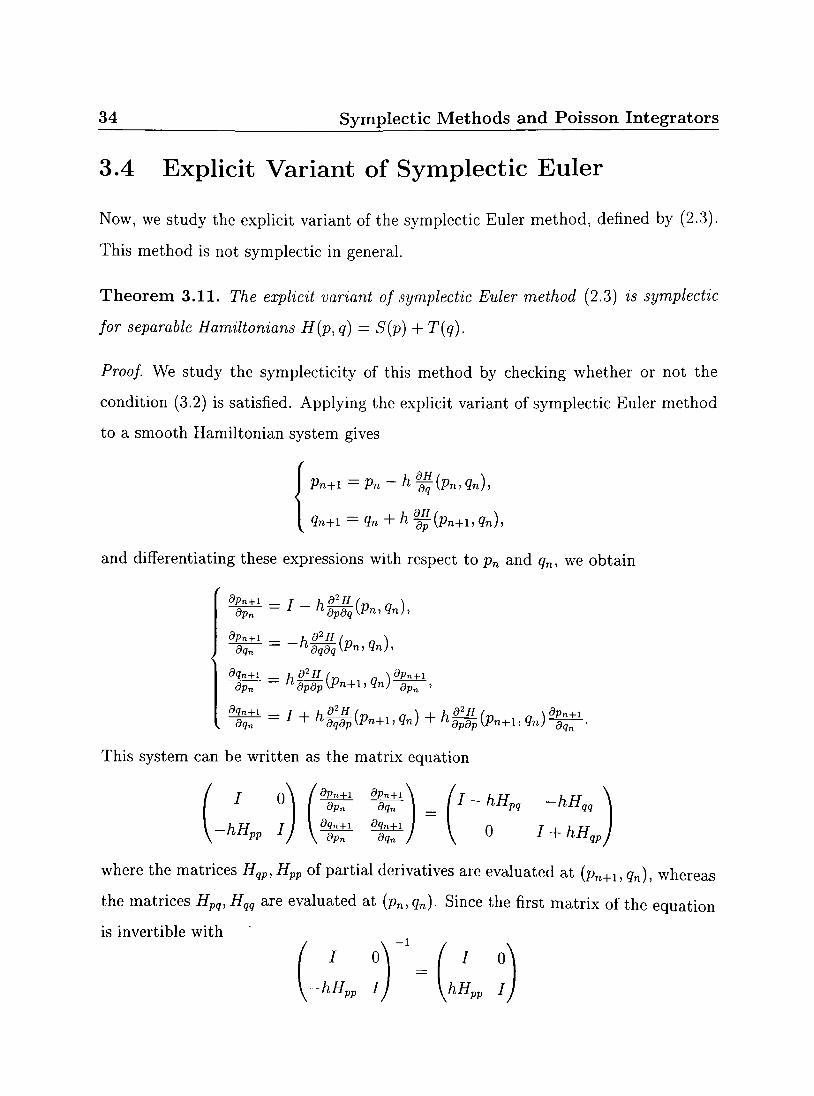
3.4 Explicit Variant of Symplectic Euler
Now, we study the explicit variant of the symplectic Euler method, defined by (2.3).
This method is not symplectic in general.
Theorem 3.11. The explicit variant of symplectic Euler method (2.3) is symplectic
for separable Hamiltonians H{p, q) = S(p) + T(q).
Proof. We study the symplecticity of this method by checking whether or not the
condition (3.2) is satisfied. Applying the explicit variant of symplectic Euler method
to a smooth Hamiltonian system, gives
Pn+i =Pn -h^{Pn,qn),
qn+i =qn + h^pL{pn+i,qn),
and differentiating these expressions with respect to pn and qn, we obtain
dP»+i = I -h^L(v a )
dq„ ndqdqWnil*n>i
d1n+\ _ L d2H l \ dpn+l
dpn ~ ndpdp\Pn+l^qnl dpn '
K dqn ^ adqdp\Pn+1'qn> + ndpdp\Pn+l^qn)-g^---
This system can be written as the matrix equation
hH*> V Y^r d^r) V ° ' + *»», where the matrices Hqp, Hpp of partial derivatives are evaluated at {Pn+i,qn), whereas
the matrices Hpq, Hqq are evaluated at {pn, qn). Since the first matrix of the equation
is invertible with
/ Q\ Y (i oN
-hHpj, 11 \hHpp I
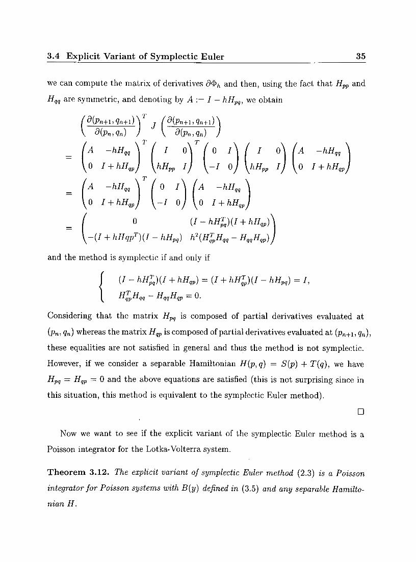
3.4 Explicit Variant of Symplectic Euler 35
we can compute the matrix of derivatives d$n and then, using the fact that Hpp and
Hqq are symmetric, and denoting by A := I - hHpq, we obtain
fd{pn+l,qn+l)\ (d{pn+i,qn+i) J
d{Pn,qn) T
I 0\ / 0 I \ I I 0\ (A -hHqq
0 1 + hHm / \-I 0 \0 I+hH
0 I + hHqpJ \hHpp I) \-I 0) \hHpp IJ \ 0 I + hHqp
A -hHqq \ ( 0 I
IP I \ ± u / \ u 2 i nllqp
0 (/ - hHjq){I + hHqp)
•{I + hHqPT){I - hHpq) h2{HT
qvHqq - HqqHqp)
and the method is symplectic if and only if
(7 - hH^){I + hHqp) = (/ + hHTqp){I - hHpq) = I,
H^pHqq ~ HqqHqp = 0.
Considering that the matrix Hpq is composed of partial derivatives evaluated at
(Pn, qn) whereas the matrix Hqp is composed of partial derivatives evaluated at (pn+i, qn),
these equalities are not satisfied in general and thus the method is not symplectic.
However, if we consider a separable Hamiltonian H{p,q) = S{p) + T{q), we have
Hpq = Hqp — 0 and the above equations are satisfied (this is not surprising since in
this situation, this method is equivalent to the symplectic Euler method).
•
Now we want to see if the explicit variant of the symplectic Euler method is a
Poisson integrator for the Lotka-Volterra system.
Theorem 3.12. The explicit variant of symplectic Euler method (2.3) is a Poisson
integrator for Poisson systems with B{y) defined in (3.5) and any separable Hamilto
nian H.
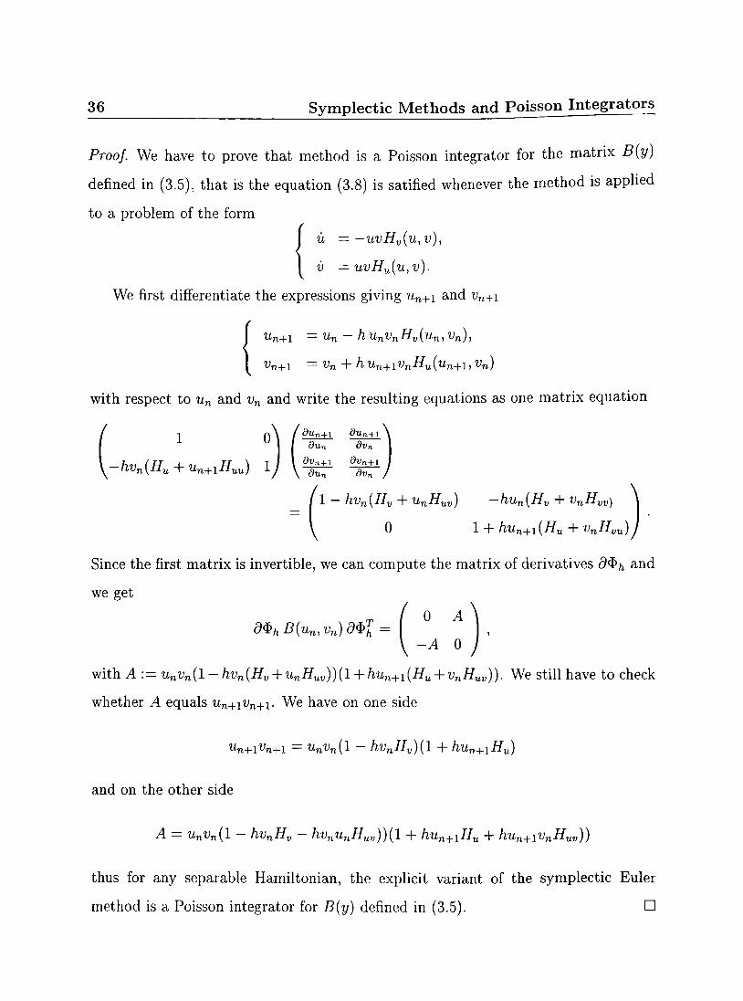
36 Symplectic Methods and Poisson Integrators
Proof. We have to prove that method is a Poisson integrator for the matrix B(y)
defined in (3.5), that is the equation (3.8) is satified whenever the method is applied
to a problem of the form
u = —uvHv{u, v),
ii = uvHu(u,v).
We first differentiate the expressions giving u n + i and vn+i
un+i = un- h unvnHv(un, vn),
vn+i = vn + hun+iVnHu{un+i,vn)
with respect to un and vn and write the resulting equations as one matrix equation
1 n \ / dun+\ dun+i j J du„ dvn
-hvn{Hu+Un+lHuu) 1) V ^ J l »g±
1 - hvn(Hv + unHuv) -hun{Hv + vnHvv)
0 1 + hun+i {Hu + vnHvu)^
Since the first matrix is invertible, we can compute the matrix of derivatives d$h and
we get
T l 0 A d$hB(un,Vn)d$T
h = \ -A 0
with A := unvn(l-hvn{Hv + unHuv))(l + hun+i(Hu + vnHuv)). We still have to check
whether A equals un+1un+1. We have on one side
Un+lVn+l = unvn{l - hvnHv){l + hun+iHu)
and on the other side
A = unvn{l - hvnHv - hvnunHuv)){l + hun+lHu + hun+iVnHuv))
thus for any separable Hamiltonian, the explicit variant of the symplectic Euler
method is a Poisson integrator for B{y) defined in (3.5). •
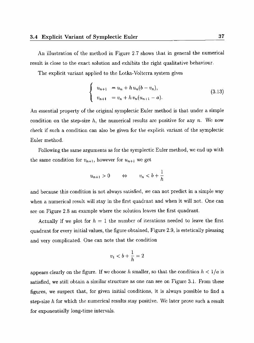
3.4 Explicit Variant of Symplectic Euler 37
An illustration of the method in Figure 2.7 shows that in general the numerical
result is close to the exact solution and exhibits the right qualitative behaviour.
The explicit variant applied to the Lotka-Volterra system gives
un+i =un + hun(b-vn), (3 13)
Vn+1 =Vn + h Vn {Un+l ~ a).
An essential property of the original symplectic Euler method is that under a simple
condition on the step-size h, the numerical results are positive for any n. We now
check if such a condition can also be given for the explicit variant of the symplectic
Euler method.
Following the same arguments as for the symplectic Euler method, we end up with
the same condition for vn+i, however for u n + i we get
un+i > 0 <=> vn <b+ -h
and because this condition is not always satisfied, we can not predict in a simple way
when a numerical result will stay in the first quadrant and when it will not. One can
see on Figure 2.8 an example where the solution leaves the first quadrant.
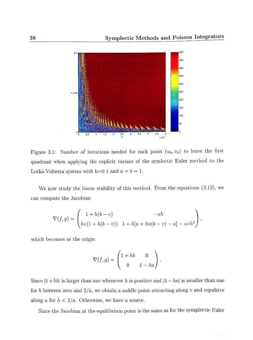
Actually if we plot for h = 1 the number of iterations needed to leave the first
quadrant for every initial values, the figure obtained, Figure 2.9, is estetically pleasing
and very complicated. One can note that the condition
vi < b + - = 2 h
appears clearly on the figure. If we choose h smaller, so that the condition h < 1/a is
satisfied, we still obtain a similar structure as one can see on Figure 3.1. From these
figures, we suspect that, for given initial conditions, it is always possible to find a
step-size h for which the numerical results stay positive. We later prove such a result
for exponentially long-time intervals.
38 Symplectic Methods and Poisson Integrators
Figure 3.1: Number of iterations needed for each point {u0,v0) to leave the first
quadrant when applying the explicit variant of the symlectic Euler method to the
Lotka-Volterra system with h=0.1 and a = 6 = 1.
We now study the linear stability of this method. From the equations (3.13), we
can compute the Jacobian
V(/,o) = ' l + h(b-v) -uh
i hv{l + h(b - v)) 1 + h[u + hu(b - v) - a] - uvh'
which becomes at the origin
V(/,<7)
Since |1 + hb\ is larger than one whenever h is positive and |1 — ha\ is smaller than one
for h between zero and 2/a, we obtain a saddle point attracting along v and repulsive
along u for h < 2/a. Otherwise, we have a source.
Since the Jacobian at the equilibrium point is the same as for the symplectic Euler
3.4 Explicit Variant of Symplectic Euler 39
method, that is
( 1 -ah V(/,s) =
\hb 1 - abh2
the conclusions are the same : for h smaller than 2/^/ab, the numerical solution is
rotating around the equilibrium point. We will see later that we need to choose h
much smaller than 2/a or 2/\fab to ensure a positive numerical solution, thus we will
have a saddle point at the origin and a center at the equilibrium point.

40 Symplectic Methods and Poisson Integrators
41
Chapter 4
Backward Error Analysis
In this chapter, we introduce the notion of backward error analysis, a very useful tool
to study the qualitative behaviour of numerical methods over long time intervals. The
idea of backward error analysis is to search for a modified differential equation of the
form
ij = f(y) + hf2(y) + h2f3{y) + ..., (4.1)
such that the solution y of this modified equation corresponds to the numerical so
lution of y = f{y), that is yn = y{nh). Of course the modified equation depends on
the method applied and usually, the series in (4.1) diverges, so one has to truncate it
suitably.
4.1 Propert ies of Symplectic Methods and Poisson
Integrators
The most important property of symplectic methods is that if such a method is applied
to a Hamiltonian system with a smooth Hamiltonian, then the modified equation (4.1)
is also Hamiltonian. Before stating this result we need to prove an important Lemma,
42 Backward Error Analysis
often called Integrability Lemma. The proof we give is essentially the same as in [5J.
Lemma 4.1. Let D C Rn be open and f : D ->• Rn be continuously differentiable, and
assume that the Jacobian f'{y) is symmetric for all y G D. Then, for every yo 6E L)
there exists a neighbourhood of yo and a function H{y) such that
f{y) = VH(y)
on this neighbourhood.
Proof. Consider y0 € D and a ball around y0 which is contained in D. Then we define
on this ball
H{y) = f (y- yoffivo + t(y - y0))dt + Const. (4.2) Jo
Differentiating H with respect to yk, the kth component of the vector u, and using
the symmetry assumption f = f^ (which implies V/fc = M-) yields dyk dyi v H J dVk
dH dyk
dt r1 df
(y) = I fkiyo + t(y - y0)) + {y- ^ ) T ^ ( y o + t{y - y0)) t
r1 d = J jt{tfk{yo + t{y-y0)))dt
= fk(y),
which proves the lemma. •
The important point of this proof is that it shows that for star-shaped regions D,
or convex sets D, the function H is globally defined : we fix y0 such that for all y in
D and all t between zero and one, we have
yo + t(y -y0) e D
and H defined by (4.2) is thus defined on all D.
Theorem 4.1. If a symplectic method $n(y) is applied to a Hamiltonian system
with a smooth Hamiltonian H : D C R2d -> R, where D is simply connected, then
4.1 Properties of Symplectic Methods and Poisson Integrators 43
the modified equation (4-1) is also Hamiltonian. More -precisely, there exist smooth
functions Hj : D —> R for j = 2, 3 , . . . , such that fj{y) = J~xVHj{y).
This result can be generalized to any arbitrary open set D, however since the
Lotka-Voltera system is defined on a convex set, we don't need to study further
symplectic methods. The proof of this theorem and the proofs of the following ones
can be found in [5]. As stated in the following theorems, the previous result can be
generalized to Poisson integrators.
Theorem 4.2. If a Poisson integrator $n{y) is applied to the Poisson system (3.4),
then the modified equation is locally a Poisson system. More precisely, for every
yo € Rn there exist a neighbourhood U and smooth functions Hj : U —> R such that
on U, the modified equation is of the form
j = B{y)(VH{y) + hVH2{y) + . . . ) . (4.3)
This result, which is only considering the local structure of the modified equation,
can be made more global under additional conditions on the differential equation.
Theorem 4.3. / / H{y) and B{y) are defined and smooth on a simply connected
domain D, and if B{y) is invertible on D, then a Poisson integrator $/i(y) has a
modified equation (4.3) with smooth functions Hj{y) defined on all of D.
Since for the Lotka-Volterra system, the matrix B{y) is invertible on ID = {y =
{u,v) : u > 0, v > 0}, whatever Poisson integrator you use to solve it, the modified
equation is globally a Poisson system. We usually call the Hamiltonian of the modified
system the numerical Hamiltonian of the original system.
44 Backward Error Analysis
4.2 T h e Symplect ic Euler M e t h o d
4.2.1 First Order Term
In this section, we derive the first order term of the numerical Hamiltonian corre
sponding to the symplectic Euler method applied to the Lotka-Volterra system,
U n . J . 1 = U„ " + 1 ~~ l-h{b-vn)
Vn+1 = Vn + hvn(un+1 - a).
The first step is to find what the method gives when we expand u(tn+i) = u(tn + h),
for h small. We consider
u(tn+i) = l-h(b-v{tn)Y '
and using Taylor series
n>0
we obtain the expansion
u(tn+l) = u(tn) Y,[W~ v(tn)) }p, (4.4) p>0
which means the term of order hp is u(6 — v)p hp.
To find the first order term of the numerical Hamiltonian, we use the ansatz
ii = f{u,v) + hf2{u,v),
v = g{u,v) + hg2{u,v),
4.2 The Symplectic Euler Method 45
where f(u,v) = u{b - v) and g{u,v) = v{u — a), and substitute it into the Taylor
expansion of u{tn+i),
h2
u{tn+1) = u{tn) + hii{tn) + —u{tn) + 0{h3)
= u{tn) + hf(u{tn),v(tn)) + h2f2{u{tn),v{tn))
+ Y[^U(tn)^(tn))u + ^{u{tn),v{tn))vj +0{h3),
= U{tn) + hf{u{tn),v{tn)) + h2f2{u{tn),v{tn))
+ \{^{u{tn),v{tn))f{u{tn),v{tn))
+ ^{u{tn),v{tn))g{u{tn),v{tn))j +0{h3).
Comparing this expansion with the one of the method (4.4) that we can write as
u(tn+1) =u + hf(u, v) + h2f{u, v)Mu, v) + 0{h3), du
we find that for an 0{h3) residual, we need f2 to satisfy
h(u, v) + - ( —(u, v)f{u, v) + —(u, v)g{u, v)j= / (u, v)-^{u, v),
in other words
1 fdf £ df_\ 1 r..,L ,2
/ 2 K v) = 2 I 'du'1 ~ ~fog) = 2 ^ b ~ ^ + UV^U ~ a^'
Similarly we obtain the Taylor expansion for vn+i ,
v{tn+l) = v{tn) + hg{u{tn),v{tn)) + h2g2{u{tn), v{tn))
+ y ( f ^ M * * ) , v(tn))fWn), v{tn))
+ ^{U{tn), V{tn))g{u{tn), V{tn))j + 0{h3),
and for v the method gives
v{tn+i) = v{tn) + hv{tn)[u{tn+1) - a],
= v{tn) + hv{tn)[u + u{b - v)h + u{b - v)2h2 H a]
= v{tn) + hv{u - a) + h2uv{b - v) + h3uv{b - v)2 + . . . ,
46 Backward Error Analysis
that is, the term of order hp is [uv{b-v)p-l}hp. Therefore, to obtain an 0{h3) residual,
we must have
g-i (u, v) + \(^{«> v)f^ v) + %^ v ) ^ «)) = ^ ( u > v ^ ^ u ) '
or
(4.5)
Putting these results together, we obtain the modified equation
u = u(6 - v) + | [u(b - v)2 + uv{u - a) ],
v = v(u - a) + | [uv(b - v) - v(u - a)2].
To obtain the numerical Hamiltonian, some algebra is needed. We first divide the
two equations of the modified system,
u u(b- v) + | [ u ( 6 - v)2 + uv{u - a)]
v v{u — a) + | [uv{b - v) - v{u - a ) 2 ] '
to obtain
d u ( u ( u - a ) + - [ u f ( 6 - i ; ) - ? ; ( u - a ) 2 ] ) =dvlu(b-v) + - [u(6-i ;)2 + m; (u -a ) ]
Dividing this equality by uv, we get
du 1 - - + - [ 2a + 6 \ u 2 —v -u ])+dv[l-- + -[a
u \ v 2 -u
62 \
- + 26- , ] j=0
and integrating it, we obtain the Hamiltonian of the modified system (4.5)
Hh{u,v) = u — a In u + — (2ua + bu —uv u a2 In u) + v — 6 In v
h v2
+ -(av - b2\nv + 2bv - —).
- H{u, v) - -[ — + uv + — - (2a + b)u - (a + 2b)v
+ a2\nu + b2\nv}.
We summarize these results in the following lemma.
4.2 The Symplectic Euler Method 47
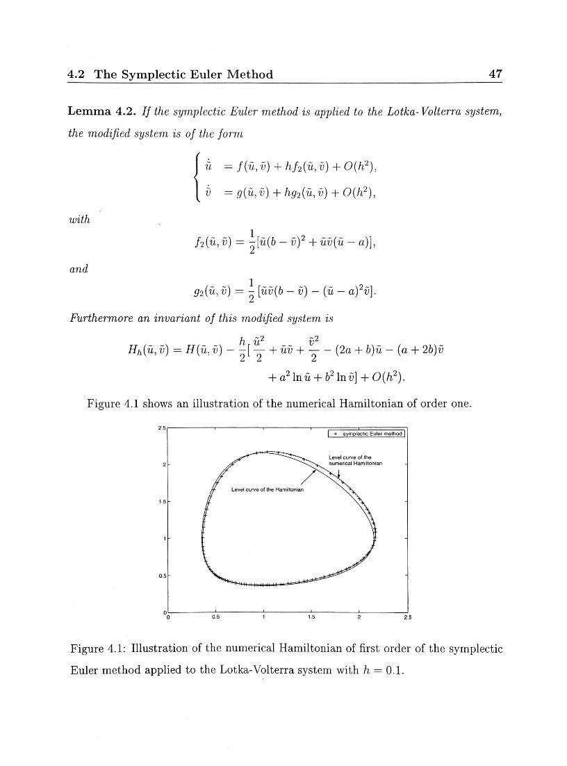
Lemma 4.2. If the symplectic Euler method is applied to the Lotka-Volterra system,
the modified system is of the form
il = f{u, v) + hf2(u, v) + 0(h2),
v = g(u,v) + hg2{u,v) + 0(h2),
with
and
f2{u, v) = -[u(b - v)2 + uv(ii - a)],
1 g2{u, v) = - [uv(b - v) - (u - a) v).
Furthermore an invariant of this modified system is
h u ii Hh{u, i)) = H{u, v) [ h ui) H (2a + b)u - (a + 2b)v
+ a2 lnu + 62lni)] + 0(/z2).
Figure 4.1 shows an illustration of the numerical Hamiltonian of order one.
4- symplectic Euler method
Level curve of the numerical Hamiltonian
Figure 4.1: Illustration of the numerical Hamiltonian of first order of the symplectic
Euler method applied to the Lotka-Volterra system with h = 0.1.
48 Backward Error Analysis
4.2.2 Second order term
Following the same steps as in the previous section, we derive the second-order term
of the numerical Hamiltonian. To do so, we use the ansatz
ii = /(u, v) + h /2(u, v) + h2f3{u, v),
v = g{u,v) + hg2{u,v) + h2g3(u,v), (4.6)
where f2 and g2 are those computed in the previous section. To compute / 3 and
g3 we need the Taylor expansions of u(in+1) and v(tn+i) up to order /z4. From the
expression giving it in the ansatz (4.6), we obtain u = f'(u,v) + hf2(u,v) + 0(h2)
and 'ii = f"(u, v) + 0{h) and thus (omitting tn, u and v when there is no ambiguity)
h2 h3
U{tn+l) = U{tn) + hil{tn) + —u(tn) + —u{tn) + 0(h*)
= u + hf + h2f2 + h2
—f+ — du dv
+ h3[h + - df df ^df2 df2 du dv du dv
1 + 6 du2 /2 + 2
d2f , d2f g + -^g2 + I i H /
d_f du dudv dv2
+ dldlg+dldg_f+dldl " du dv dv du dv dv
+ 0{h4).
This result (and the following ones) can be easily obtained using Maple. To obtain a
residual of order /i4, we simply have to set
/3(u, v) = -u(b - v)3 + uv(--(u- a)2 + -(u -a)(b-v) + -u(b - v) J.
Similarly, we obtain the expression for a3,
9z(u,v) = -v{u-a)3 + uv(-(b-v)2- -{b-v)(u-a) + ~v{u - a) J.
The next step is to consider u/v, where u and v are given by the ansatz (4.6) and
/3 and o3 are the ones we just derived. After simplifications, we obtain the numerical
4.3 The Structure of the Numerical Hamiltonian 49
Hamiltonian
Hh = H{u,v)-^ 2 9
U V + uv + — -(2a + b)u - (a + 26)i; + a1 In u + 6 In v
h2
+ y u3 v3 3 u2 3 v2
— + u2v + uv2 + — - (3a + - & ) — - (2a + 26)uu - (-a + 36) — O O Z ^ A Li
3 3 + (3a2 + -ab + b2)u + {a2 + -ab + 3b2)v - a3 In u - 63 ln(v)
Li LI
Higher order terms can be computed following the same procedure.
+ 0{h3).
4.3 The Structure of the Numerical Hamiltonian
As one can see from the expansion of the numerical Hamiltonian we just derived, it
seems that each term of the expansion consists of a sum of a term in In u, one in In v
and a polynomial in u and v. It is interesting to study the structure of this expansion
further, which we do in this section. More precisely, we prove that the term of order
n of the expansion is of the form
hn
( an+1 lnu + 6n+1 In v + polynomial in u and v ) . (4.7)
Theorem 4.4. When we use the ansatz
u = f + hf2 + h2f3 + ... + hnfn+1,
v = g + fg2 + h2gz + ... + hngn+l.
the coefficients fn+i and gn+i are of the form
(4.8)
fn+i = -—Tu(b ~ V)U+1 +uvx Pn+l (u, v) (4.9) lb | 1
and (-l)n
gn+i = -TTV(U ~ a ) " + 1 +uvx Qn+i (w, v) (4.10) ft I X
where Pn+\ and Qn+i o-r& polynomials.
Once this theorem is proved, a simple manipulation yields the numerical Hamilto
nian. However before proving this theorem, we first need to establish several lemmas.
50 Backward Error Analysis
4 . 3 . 1 N o t a t i o n s
To simplify the expansion of / n + 1 and gn+1, we introduce some notation. We show
the details only for the functions ft, similar notations can be easily deduced for the
functions &. We may often, to simplify formulas, denote / by / i , so that fi is well-
defined for i = l,...,n + 1. Usually we use the notation duf to denote the partial
derivative of / with respect to u, whereas the dot and the prime correspond to the
derivative with respect to t.
From the ansatz (4.8), one can find the higher order derivatives of u with respect
to t :
ii = /{ + hf2 + ... + hnfn+l, u = f; + hft + ... + hnf'n'+l, etc.
Since fi is a function of u and v, we have
fl = dufiu + dvfiv, (4.11)
which becomes, when we substitute the ansatz (4.8) into it,
fl = fdufl+gdvfl + h{f2dufl + g2dvfl) + ... + hn{fn+idufl + gn+idvft)- (4-12)
Since each derivative of the function fi with respect to t is a partial sum of a series
in h, we introduce a new notation, /,- •, to denote each term of the sum,
n
fi = fi + hf'u2 + ... + hnf'hn+1 = ] T Vfld+l. j=Q
Similarly, we introduce the same notation for the higher derivatives,
/ f = f$ + hf$ + ... + h»fW+l = JT Vf$+l, for k = l...n. (4.13) 3=0
In other words, f\J corresponds to the term of order h^~l of the fcth derivative of fi
with respect to t.
4.3 The Structure of the Numerical Hamiltonian 51
4.3.2 Der iva t ion of fn+\ and gn+i
(k)
The first step to prove Theorem 4.4 is to express fn+i and gn+\ as functions of f\J
and g(*]. Lemma 4.3. In the notation of (4.13), we have
rn-k+l
/„+1 = u(b - „r> - Y, JX^TY ( E /£L-,-+»), fi»-»> i k=i v ' ' v i=i '
Proof. Using the notation introduced in (4.13), one can write down explicitly the
expansion of u{tn+i):
u{tn+i) =u + hu+^u+... + ^ - ) + Y ^ Y u ^ + 0{h^2) 2! n! (n + 1)!
= u + h{f + hf2 + h2f3 + ... + hnfn+l)
+ !$(f, + hti + --- + hn-1fn)
+ r{f{n-1) + hft1)) n!
+ 7 ^ r T ( / ( n ) ) +0{hn+2) (n + 1J!
= u + M + A2 (/2 + i / i ,^ + />3 (/3 + i(/f>2 + / y + i.tffl)
+ ^ (/4 + |( / | ,3 + /2,2 + /i,l) + ^ ( / ^ + tf.l) + ^ j /S )
+ + 1 (/n+1 + ^ ( / i l B + / i „ - i + • • • + /A,!) + | ( /Cn -1
n,Ul,2 +/2.1 ) + ( „ + ! ) + • • • + tf-1.1) + • • • + iiW* + /2" ) + TZXTuiW
+ 0{hn+2).
52 Backward Error Analysis
From this expansion, we obtain an explicit expression for fn+i as a function of the
derivatives of fi, i = 1,..., n: since the method gives
un+i = u„ J ^ [/i (6 - vn)]p,
p>0
we should have
/ . „ = „ ( i - , r > - ^ ( ^ + . . . + ^ l ) - . . . - ^ ( / ( - 2 - n + / g - ' ) ) _ _ 2 _ y < j ) , (414)
for n > 1. A similar argument is used to derive gn+1. The only difference comes from
the expansion of the method; we have
Vn+i =vn + hv(u - a) + ^2 iuv(b ~ v)p~l]hp, P>2
therefore, we obtain, for n > 1,
* „ = »(6 - „)• - i(9;,„ +...+,;,,) - . . . _ I(s(»-» + s(»-')) _ j ^ j w ,
and the lemma is proved. [j
This result, although interesting, is not directly usable, since the derivatives of
fi and gi become more and more complicated. A method enabling us to find the
functions fi and g{ explicitly is to express the functions in terms of trees. More
details and results about this method can be found in [5] (Theorem 9.4 on page 319)
In the next chapter we give an expansion of / n + 1 as a function of Lie derivatives. Yet
even if we are not able to find fn+i and gn+l explicitly in a simple way, we can use
those results to study the structure of the functions fi and gt and prove Theorem 4 4
The advantage of this notation is that it is easier to follow exactly what each term
corresponds to.
4.3 The Structure of the Numerical Hamiltonian 53
4.3.3 The Structure of tfk) and g\k) J»,3 Ji,3
From (4.14), we see that / n + 1 consists of a linear combination of derivatives with
respect to t of the fi. When we replace these derivatives by their counterparts com
posed of derivatives with respect to u and v, we obtain a polynomial whose terms are
a product of fi and gt and their derivatives, but the essential observation is that, as
soon as there is at least one derivative with respect to u in a product, then at least
one fi appears in this product, and similarly a factor #,• is necessary if the product
contains a derivative with respect to v. We have exactly the same result for gn+i-
By our induction hypothesis, we have for k = 1,..., n,
dufk = 7(6 — v)k + v x polynomial of (u, v), k
dvfk — —u(b — v) + u x polynomial of (u, v),
and
dugk — {—1) v{u — a) + v x polynomial of (u, v),
dvgk = - (u — a) + u x polynomial of (u, v). k
Then, the higher derivatives with respect to u (and only u) of fk and gk are all of the
form v x polynomial of (u, v), and the higher derivatives with respect to v (and only
v) of fk and o are all of the form u x polynomial of (u, v).
Because we want to prove (4.9) and (4.10), we are only interested in terms that
do not contain the product u x v : any term containing this product is included in the
second part of (4.9) or (4.10). We just saw that any product containing a derivative
with respect to u contains also one /,- and any product containing a derivative with
respect to v contains also one gi, thus any product containing a derivative of u and v
contains also one fi and one gi. Moreover, since, by the induction hypothesis, fz is of
the form u x a polynomial of (u, v) and & is of the form v x a polynomial of (u, v),
we know that any product containing a derivative with respect to u and v is of the
form u x u x polynomial of (u, v).
54 Backward Error Analysis
Moreover, apart from duf{, the derivatives of f{ and gt with respect to u are of the
form v x polynomial of {u,v), so multiplied by a function /, we obtain again u x vx
a polynomial of (u,v). Similarly, the derivatives of fi and gt with respect to v are,
apart from dvg%, of the form u x polynomial of (u, v), so multiplied by gi} we obtain
u x vx a polynomial of (u,z;).
Consequently, the only terms not included in the second part of (4.9) or (4.10)
are the ones composed only of /,'s and/or first derivatives of fi with respect to u, or
composed only of g^s and/or first derivatives of gi with respect to v.
Our task is now to find where these terms appear in f\J and ghj. From (4.12),
we already know that
f'ij = dufifj + dvfigj,
and
g'ij = duglfj + dvgigj.
To find the higher derivatives, we use (4.11) to obtain
/ " = duufi u2 + 2duvfi uv + dvvfi v2 + duft il + dvfz v,
and
g" = duugi ii2 + 2duvgz uv + dvvgx v2 + dug{ u + dvgt v,
but as we said before the only terms we are interested in are the ones containing
only the first derivative with respect to u of fi, or the ones containing only the first
derivative with respect to v of #;. So we should write
/ " = dufi u -I- other derivatives of fu
and
g'l — 9vgi v + other derivatives of g^.
Similarly, we obtain for the next derivatives
f\ ' = dufi u^ + other derivatives of fi,
4.3 The Structure of the Numerical Hamiltonian 55
and
g\ = dvgi v^k' + other derivatives of gx.
Since u^ and v^ are given by
and
„<'> = /<*-»+ */<*-•> + ... + /,»/£-»,
»<*» = si '""+ Asi*-"+ ... + * - & " .
we obtain, using the notation introduced in (4.13),
?(*+i) _ / i r ; = ^ f i c(fc) i r(fc) (*)
J\,j "+" / 2 , j - i I " • • • "t- J j , l + functions of other derivatives, (4.15)
and
sir= dv9i (k) , (*) . , CO
9\J + Aj-i + •••+ 9),{ + functions of other derivatives.
From this last result, we can obtain f>j and g\J by induction on k.
Lemma 4.4. In the notation of (4.13), we have
^(fc+i) _ _ Q(k+i) u^ _ vy+j+k _|_ uy x p0iynomiai {n u and v^
and
pj/c+1) = {-l)i+j -Cf+l) v{u - a)i+j+k + uv x polynomial in u and v,
where Cf} is defined recursively by C) -1/j and
c) (fc+1) V ^ 1
r(k)
Proof. As suggested by the expansion (4.15) of /£ • ', we use an induction argument.
We first consider the case A; = 0 where we have
f = dufi fj + ... = -{b- v)l-u{b -v)j + uv... = -u{b - v)i+j + uv..., % j ij
56 Backward Error Analys is
and we define C' to be C\ := - so that
fl3 = -C'u{b-v)^ + uv....
Now we consider
f"j = dutifij+r2,-i + ...+rhi\ + 3
= dufi 2_^ fpj+i-p + • • • P=i
j
= W-vyti1-c'^-Pu(b-vr+H1-p+---%
P=iP
= 7E^i + i -p«(6-«) i + i + 1 + - . 1
P = i p
so defining C" := £ J = 1 \ C']+i-P > w e obtain
/ ' ' = - C ; ' u ( 6 - i ; ) ^ + 1 + u z ; . . . .
This example suggests to define C- + by
r(k+l) ._ V^ V(/=) ° J — 2^ D°J+I-P •
p = l y
Then, using the induction hypothesis we get
P = l
= ~(b - ^ £ - C ^ ! _ p u{b - w)P+i+i-i»+'-i +
P=I P
lA 1
P = i i
i = - d ' + 1 ) u(b - v)l+]+l + uv . . . ,
z J
and the first part of the lemma is proved.
4.3 The Structure of the Numerical Hamiltonian 57
A similar procedure leads us to the formula corresponding to g\j . For k = 0,
we have
9iJ = 9jdv9i + •••
(_l)(;-i) (-1V+1
= - - (u - a)- -—v(u - a)3 + uv i 3
(-lY+i . . = - —v(u - a)l+3 +uv...
= {-l)l+3-C'v{u-a)i+3, n J
and using the induction hypothesis, we obtain
i
9?r)=dv9>Yi9pi-p+---p=i
uv = ( 1 ) Z " (u - a)1 ^ ( - 1 ) P + J + 1 - P - Cf+l_p v{u - a)
p+3+l'p+l-1 + 1 P=i p
= ^±l-Cfll_pv{u-ay^+uv...
= {-iy+J - cf+l) v{u - a)l+j+l + uv..., i J
which concludes the proof. •
4.3.4 Proof of Theorem 4.4
The first step for proving Theorem 4.4 consists of checking whether or not the induc
tion hypotheses are satisfied for n = 0 and n = 1. We already know from the previous
sections that / = u(6 - v), g = v{u - a),
h = -u{b-v)2+ uv-{u-a) and g2 =--v{u - a)2 + uv-{b - v),
58 Backward Error Analysis
so they satisfy the induction hypothesis (4.9) and (4.10). Then, using the results of
Lemma 4.4, we have
f(k) - \n{k) ii(h-vV+n-k-j+2+k-l , Jj,n-k-j+2 — • ^n-k-j+1 U\° V) -+UU .. . J
1 1( fc) n.fk „,\n+l = -ci:>U{b-vr^+uv..., so that
E C - i « = E 7c&_,««(»-«)"+I+ «»••• j=l j=l
(n-k+1 -. \
= C(n
k_X u(b - v)"+1 +uv....
Substituting this into the expansion of fn+i given in Lemma 4.3 we obtain
z„+1 = u(b - „ r ' - J2 jj^jy {clnh_\'X(b - «>"+i + uv..),
= (i - i : cfcTi)! cits,) «(* -»)-« Similarly, we have for gn+1
fc=l v ' / ' V j = i /
= u„(i -»)" - E (^Tji ( " E ' ( - I ) " - ' JC<V,-+»»(« - «)"+1 + «»•••)
= E-5rTTjTc^,«(«-<.r+1+™....
+ Uf
_ ( - l ) n ^(fc+j
fc=l
The parts we denoted by "+uv..." in the above results are polynomials, so it only
remains to show that n
•i(k+i) _ 1
^ (k + l a
^ (fc + 1)! n~fc+1 n + 1
4.3 The Structure of the Numerical Hamiltonian 59
and
v (-ir f c r(*+p = ( - i )n
^ (fc + 1)! n~k+1 n + 1
Lemma 4.5. / / we define
C f = J <^ C<t+1» = y j i C< % , ; > 1 , p=l P
the two following identities hold
n i n I i \ k 1
^(k + l)\ n~k+1 ~ n + l ' ^ (Jfc + 1)! "-*+1 " n + 1 ^ ( * + l)! / c = l
Proof. The key is to introduce the generating function (suggested by Ernst Hairer)
a(fc)(C)=E^UJ-j>0
For fc = 1, we obtain
and on the other hand we have
„<» «)«<»> (o = E M ' ^ - U <' = E ^ t 1 1 cj = o<t+1)(o, j>0 p-0 j>0
therefore
From this identity we obtain
ln(l ~ C) c
fc>2 ?>0 fc>2
as well as
EE^^^^i-^-or
(4.16)
(4.17) fc>2 j > 0 fc>2
60 Backward Error Analysis
If we define n to be n — j + k, the left-hand side of (4.16) can be rewritten as
EE^Sc , + l = EE k>2 j>0 k>2 n>k
EE fc>l n>k
(-iy k\
i(k) U n - f c + l s.
E 71>1
(-l)fc + 1 (fc + l ) + 1
(fc + 1)! °"- f c + 1^
(_l)*+i a (fc+i)
^ (fc + l ) !^ n - f c + 1 -n+1
Similarly the left-hand side of (4.17) can be rewritten as
E V ±_r{k) rj+k _ V^ Y^ l r(k+l)
^ k> i + 1 ^ ~ ^ ^ (k + lV n~k+]
k>1 j>0 ' n > l L k=l V ' '
Now if we consider the right-hand side of (4.16), we have
E rr [ l n ( ! - 0 ]* = exp(ln(l - 0 ) - 1 - ln(l - C)
C n+1
fc>2
c2 c3
= l - C - l - l n ( l - C ) = y + y + n+1
^ n ^ n + 1 n>2 n > l
and the equation (4.16) becomes
E n > l
y^ {-L) c(k+i) ^(k + iy. n~k+1
c+i = ^ C n+1
n > l n + 1'
so that we have V^ (-l)k+1 g(k+l) _ 1
^ (fc + l)! "~fc+1 n + 1 '
which is the first identity we wanted to prove. Finally since the right-hand side of
(4.17) can be rewritten as
E ^ [ - M l - C ) ] f c = ~ - l + l n ( l - C ) fc>2 c
= 1 + C + C2 + 1 n
2 3
= E n > l
n + 1 n+1
4.3 The Structure of the Numerical Hamiltonian 61
the equation (4.17) becomes
E n > l
n
V r{k+l)
^(k + iy n~k+l - ( * + !) and we obtain the second identity.
-n+1 E n > l
n n + 1
c n+1
D
4.3.5 Conclusion
To find the numerical Hamiltonian, we consider the quotient
u = f + hf2 + h2h + • • • + hnfn+1
v g + hg2 + h2o3 + . . . + hngn+i'
which gives
du (g + hg2 + h2g3 + ... + hngn+l) = dv (/ + hf2 + h2f3 + ...+ hnfn+1).
We are only interested in the part of order hn since we want to prove (4.7), that is we consider
— ( fn+idv - gn+idu J = 0, uv \ J
and using the expressions of / n + i and gn+i given by Theorem 4.4, we can write
• ( - ! ) " 1 1 1 du\ ^ - - ( u - a)n+1 + Pn+i{u, v))-dv( —-r-{b - v)n+1 + Q n + 1 ( u , v ) ) = 0 ,
\n +1 u / \ n + lv J
which becomes when we expand the products
/ ( _ i W _ a ) " + i . \ / i bn+l ~ \ du[±—:> S—I + Pn+1{u,v)) -dv(—- + Qn+l{u,v)} =0.
\ n + l u / \ n + 1 u /
To obtain the term of the numerical Hamiltonian, we simply integrate this equality
(which is possible by Theorem 4.3), and we get
• an+1 lnu -bn+l lnu + polynomial in (u, v) — Const., n+1 n+1 K v ;
and then the new term of the expansion of the numerical Hamiltonian is of the form
hn
-[an+l lnu + 6n+1 \nv + polynomial of u and v],
which is what we wanted to prove.
62 Backward Error Analysis
4.4 The Explicit Variant of the Symplectic Euler
Method
4.4.1 First Order Term
We now derive the term of order h of the numerical Hamiltonian corresponding to
the explicit variant of the symplectic Euler method. Considering the Lotka-Volterra
system (1.1), the variant of the symplectic Euler method is given by (2.3) with
f{u,v) = u{b - v) and g{u,v) = v{u - a). To find the first order term of the
numerical Hamiltonian, we use the ansatz
ii = f{u,v) + hf2{u,v),
ii = g(u,v) + hg2{u,v).
Since we have
h2
u{tn+l) = u{tn) + hu{tn) + —u(tn) + 0{h3)
= U{tn) + hf{u{tn), V(tn)) + h2f2{u{tn),v{tn))
+ y (j£.(u(tn), v{tn))it + -^{u(tn),v{tn))iXj + 0(h3),
= u(tn) + hf(u(tn), v(tn)) + h2f2{u{tn), v{tn))
h2 fdf + y ( ^M*n),v(tn))f{u(tn),v{tn))
and the method gives
+ -^{u{tn),v{tn))g{u{tn), v{tn)) J + 0{h3),
u{tn+1) = u{tn) + hf{u{tn),v{tn)),
we must have
f2{u, v) + - ( —(u, v)f{u, v) + — (u, v)g{u, v)\ = 0 ,
4.4 The Explicit Variant of the Symplectic Euler Method 63
to obtain an 0{h3) residual, that is
f2{u,v) = --(—{u,v)f{u,v) + —{u,v)g{u,v)J,
= — -[u(6 — v)2 — uv{u — a)].
Similarly we have for v (in+i)
v{tn+i) = v{tn) + hg(u{tn), v{tn)) + h2g2(u{un), v{tn))
i 2 / ct
+ ^\J^{u{tn),v(tn))f{u(tn),v{tn))
+ -£(u(tn),v{tn))g{u(tn),v{tn))\ +0{h3),
but since for v the method gives
V{tn+l) = V{tn) + hg{u{tn+1),v(tn)),
= v{tn) + hg{u{tn) + hf(u(tn), v{tn)) + 0{h2), v{tn)),
= v(tn) + hg{u{tn), v{tn)) + h2-£{u{tn), v{tn))f{u{tn), v{tn)) + 0{h3),
the condition g2 must satisfy is
52(w,v) + - f ^ ( u , w ) / + —(u,t;)aj = —{u,v)f{u,v),
that is
do lfdg dg \ ldg ldg 92{u,v) = -f--\^-f + -g) = 2 ^ - 2 ^
= - [uv{b — v) — (u — a)2w].
Finally, we obtain the numerical Hamiltonian of the Lotka-Volterra system
h u v
Hh = H{u, v)--[ — + uv- — -{2a + b)u - (a - 2b)v
+ a 2 l nu -6 2 l n t ; ] + 0(n 2) .
We summarize these results in the following lemma.
64 Backward Error Analysis
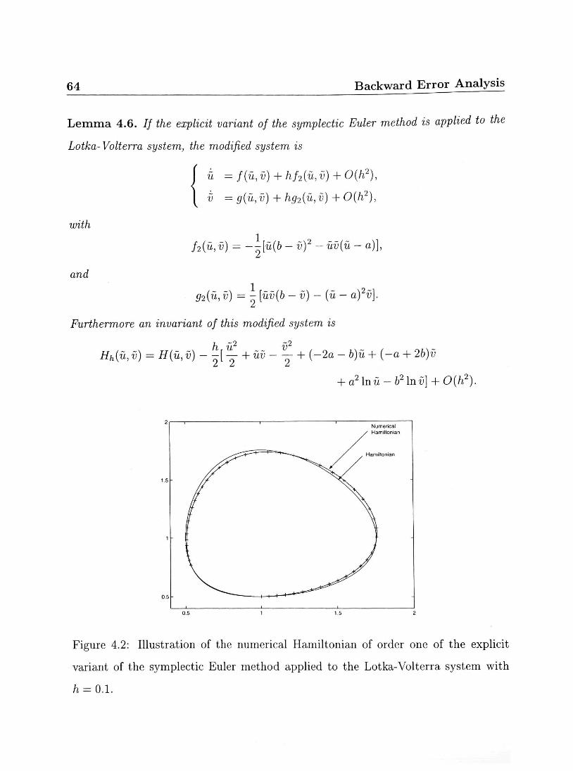
Lemma 4.6. If the explicit variant of the symplectic Euler method is applied to the
Lotka- Volterra system, the modified system is
with
and
u = f(u,v) + hf2(u,v) + 0{h2),
i) =g(u,v) + hg2{u,v) + 0(h2),
/2(u, v) = --[u(b - v)2 - uv(u - a)],
92{u, v) = - [uv(b -v)-(u- a)2v}.
Furthermore an invariant of this modified system is
h ~2 ~2
Hh(u, v) = H{u, v) - - [ y + uv - — + (-2a - b)u + ( -a + 2b)i)
+ a2\xvu-b2\iiv}xO(h2).
Figure 4.2: Illustration of the numerical Hamiltonian of order one of the explicit
variant of the symplectic Euler method applied to the Lotka-Volterra system with
/i = 0.1.
4.5 Structure of the Numerical Hamiltonian 65
4.5 Structure of the Numerical Hamiltonian
As one can see from the expansion of the numerical Hamiltonian we just derived, it
is very similar to the one we derived for the symplectic Euler method. We can prove,
following the same steps as in Section 4.3, that each term of the expansion is of the
form hn
[ a n + 1 l n u + ( - l ) n 6n+1 lnu + polynomial of u and v).
The theorem corresponding to Theorem 4.4 is the following.
Theorem 4.5. The coefficients fn+\ and gn+i are of the form
and
fn+i = ——-u(6 - v)n+1 + uv x Pn+i(u, v) n + 1
gn+i = — — - v { u - a ) n + l +uv x Qn+l{u,v),
where Pn+i and Qn+i are polynomials, when we use the ansatz
u = f + hf2 + h2f3 + ... + hnfn+1,
v = g + fg2 + h2g3 + ... + hngn+1.
The expansion of u{tn+i) given in the proof of Lemma 4.3 is still valid, however,
since the method gives
Un+1 = Un + hf{un,Vn),
with no term of order hn, n > 1, the term of order hn in the expansion of u(£n+1)
vanishes, and we obtain
/n+1 = - y ( / l , n + ••• + /n,l) - ••• ~ ^j(/l,2 + f2,l ) ~ / + 1)!^U
/n—k+1
^ (k + 1). N . , k=i y ' N j=i
For vn+i, the method gives
= - E (T^W ( E f$-k-3+2) > for " > 1-
vn+i =vn + hg{un+i, vn) = vn + hg{un + hf{un, vn),vn),
66 Backward Error Analysis
which gives with a Taylor expansion
/ h2
Vn+i = vn+ hlg + hdugii+ — (duug u2 + dug u) +
h3 \ -^{duuUgu3 + 3d u ugiiu+ dug u) + ... 1,
but since we know that duug and the higher derivatives of g are zero, this becomes
vn+l =Vn + h(g + hdugii + ^-dugu + ^dug U+... + ^jduguMj + 0(hn+2).
We can rewrite this expansion as
/ n2 /j3 ^n \
^n+i =vn + hg + hdug I hit + —ii + —ii + ... + — u(n) j + 0(hn+2),
which is very similar to the expansion of u{tn+i) derived in the proof of Lemma 4.3,
and it becomes
vn+i = vn + hg + h2dugfx + h3dug I f2 + —f[A j
+ ^ p ( / 3 + ^(/{,2 + /2,l) + ^ ' , l )
+ ^ + ^ ( / n + ^ (/(,„_! + ••• + / ;_! ,X) + ^{fl,n-2 + • • •
+ f" ) + + _ (f(n-2) , An-2), J_ f(n-l)\ ••• + /n-2,J + ---+ ^ _ ^,Ul,2 +/2.1 J + ^ / l . l J
+ 0{hn+2).
By the induction hypothesis, we have / m + 1 = - £™=1 ^ y y 2~2T=ik+1 fj*i-k-j+2 f o r
m = 1 , . . . , n — 1, so we obtain that all the terms of order hk, for k = 3 to n + 1 will
vanish, so that the method becomes
"n+1 = vn + hg + h2dugfx + 0(hn+2).
4.5 Structure of the Numerical Hamiltonian 67
Therefore, we obtain, for n greater that 2, the function gn+\, essentially the same as
/ n + 1 ;
1 / / , , I \ 1 / (n- l ) , ( n - l ) \ 1 (n) 9n+l = --[{gl,n + ---+9n,l)------Ml,2 + 92,1 0 ~ (^T^Jf^l.l »
n-k+1
E(fc+l)| I E ,n fc=l V ; V j=l
-fc-j+2
Then, considering the remarks made in Section 4.3.3, we easily obtain the following
lemma.
Lemma 4.7. In the notation of (4.13), we have
fij+ = (—l)l+j -Cj u(6 - v)l+j+l + uv x polynomial in u and v,
and
p-j+ 1 ) = ( - l ) l + J + 1 -Cf v(u - a)l+j+l + uv x polynomial in u and v,
where C- is defined in Lemma 4-4-
Now we can prove Theorem 4.5: one can easily check that the induction hypotheses
are satisfied for n = 0 and n = 1, then Lemma 4.5 and Lemma 4.7 conclude the proof.
To find the numerical Hamiltonian, we consider the quotient u/v, which yields, as in
Section 4.3.5,
— I fn+idv - gn+idu I = 0, uv \ /
and using the expressions of fn+i and gn+i we just derived, we can write
du\ (u - a)n+1 + Pn+i(u,v)\ - dvl^--(b - v)n+l + Qn+i{u,v)) = 0, n + 1 u
which gives, if we expand the products,
/(-l)n (_a\n+l _ \ / ( - l ) n 6 n + 1 - \ du( 1, +Pn+i(u,v))-dv({--)- + Qn+l{u,v) = 0 .
\ n + l u / Vn + l i ; /
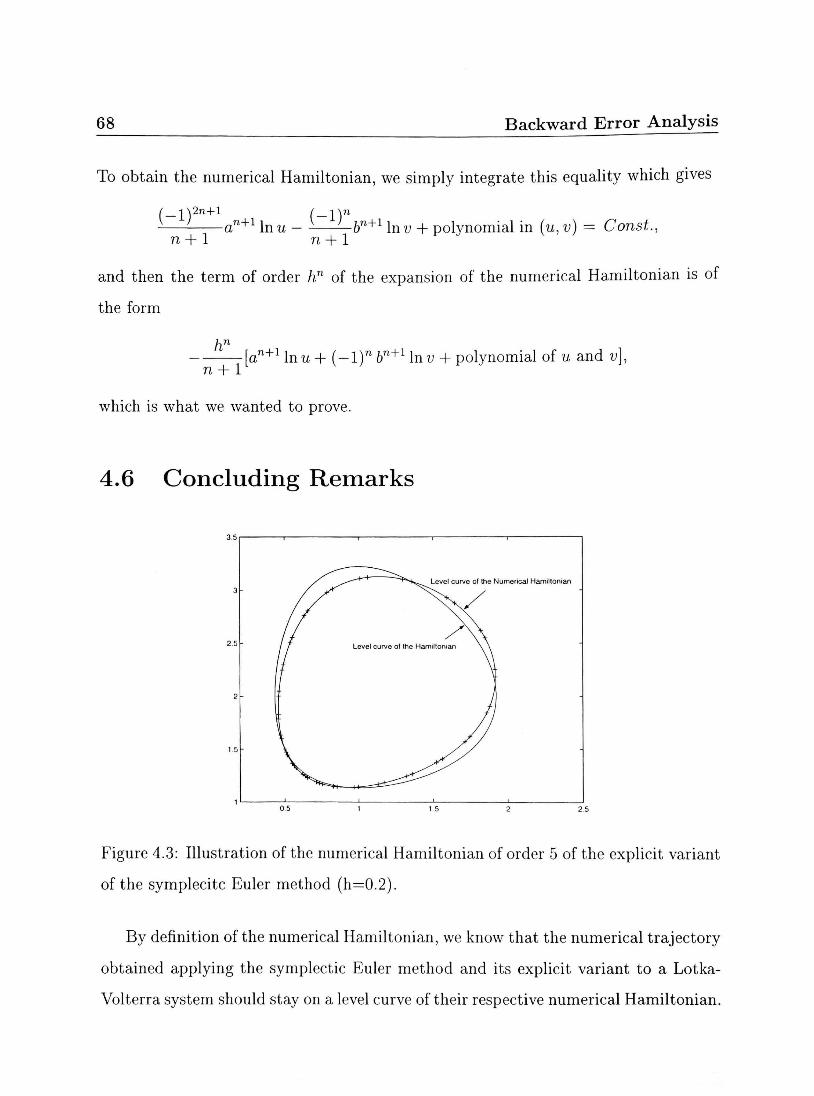
68 Backward Error Analysis
To obtain the numerical Hamiltonian, we simply integrate this equality which gives
(-1) 2n+l (-1)" an+l lnu - - 6 n + 1 lnu + polynomial in (u,v) = Const., n+1 n+1
and then the term of order hn of the expansion of the numerical Hamiltonian is of
the form
hr
n + 1 [an+l lnu + (-1)" 6"+1 lnu + polynomial of u and v],
which is what we wanted to prove.
4.6 Concluding Remarks
Level curve of the Numerical Hamiltonian
Figure 4.3: Illustration of the numerical Hamiltonian of order 5 of the explicit variant
of the symplecitc Euler method (h=0.2).
By definition of the numerical Hamiltonian, we know that the numerical trajectory
obtained applying the symplectic Euler method and its explicit variant to a Lotka-
Volterra system should stay on a level curve of their respective numerical Hamiltonian.
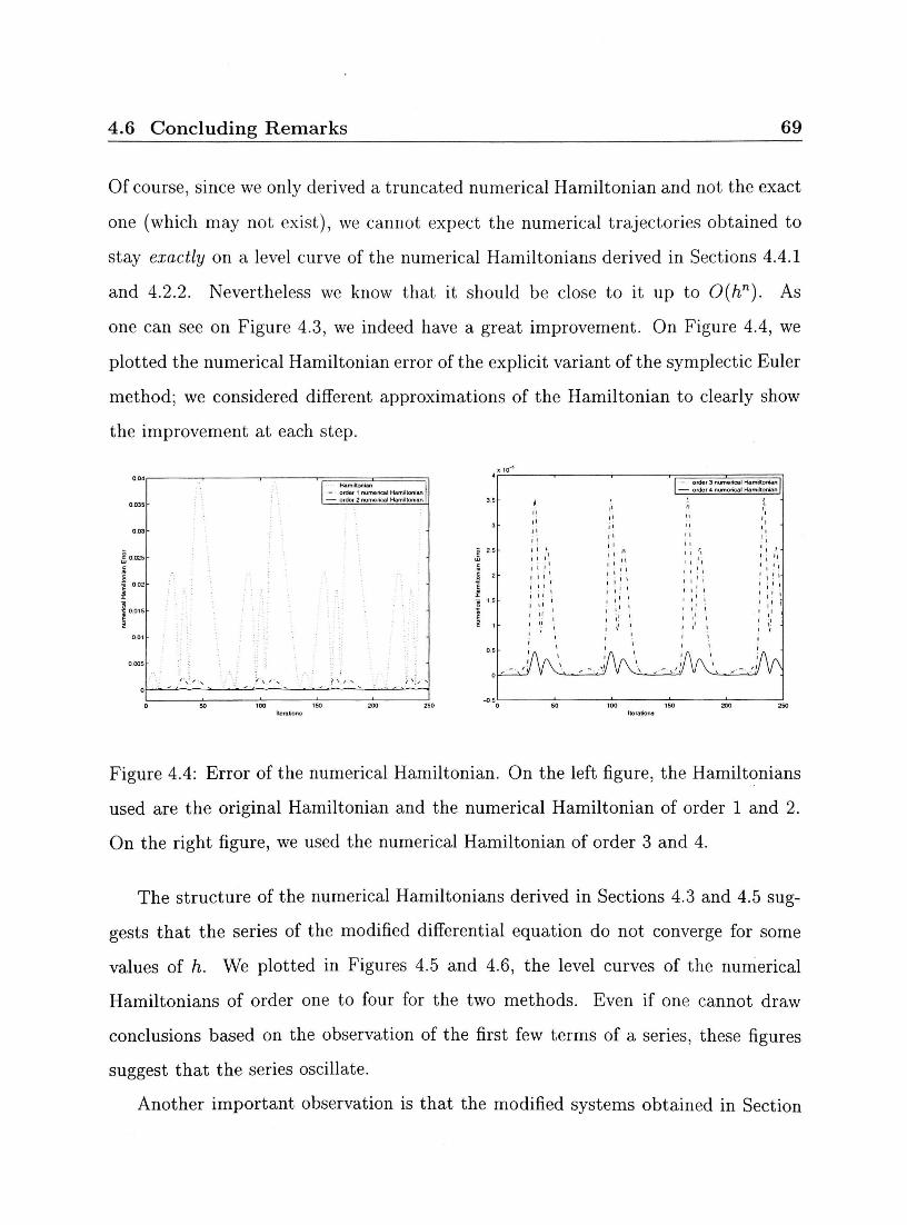
4.6 Concluding Remarks 69
Of course, since we only derived a truncated numerical Hamiltonian and not the exact
one (which may not exist), we cannot expect the numerical trajectories obtained to
stay exactly on a level curve of the numerical Hamiltonians derived in Sections 4.4.1
and 4.2.2. Nevertheless we know that it should be close to it up to 0{hn). As
one can see on Figure 4.3, we indeed have a great improvement. On Figure 4.4, we
plotted the numerical Hamiltonian error of the explicit variant of the symplectic Euler
method; we considered different approximations of the Hamiltonian to clearly show
the improvement at each step.
i i ° i I " •
Hamiltonian — order 1 numoncal Hamiltonian
order 2 numerical Hamillonian
y •
,
ii ii i i 11 i i i i i.
i i ' i
! i i ' i < ' 1 '! , i 11 I H 1 " ; ' '
ii i ' ij 11 j i
1 j j !
1 I
1 1
I — order 3 numerical Hamdtoman 1 | order 4 numerical Hamiltonian [
' 1
(! 1; il , '
I I , !
i i , !
I I ' '
1 ' , ! i i i • . 1 1 i •
i ' ' '" !!'! ' ' ' ' • 1 ' >' '
! 'i '. j ) • ' \ i
Figure 4.4: Error of the numerical Hamiltonian. On the left figure, the Hamiltonians
used are the original Hamiltonian and the numerical Hamiltonian of order 1 and 2.
On the right figure, we used the numerical Hamiltonian of order 3 and 4.
The structure of the numerical Hamiltonians derived in Sections 4.3 and 4.5 sug
gests that the series of the modified differential equation do not converge for some
values of h. We plotted in Figures 4.5 and 4.6, the level curves of the numerical
Hamiltonians of order one to four for the two methods. Even if one cannot draw
conclusions based on the observation of the first few terms of a series, these figures
suggest that the series oscillate.
Another important observation is that the modified systems obtained in Section
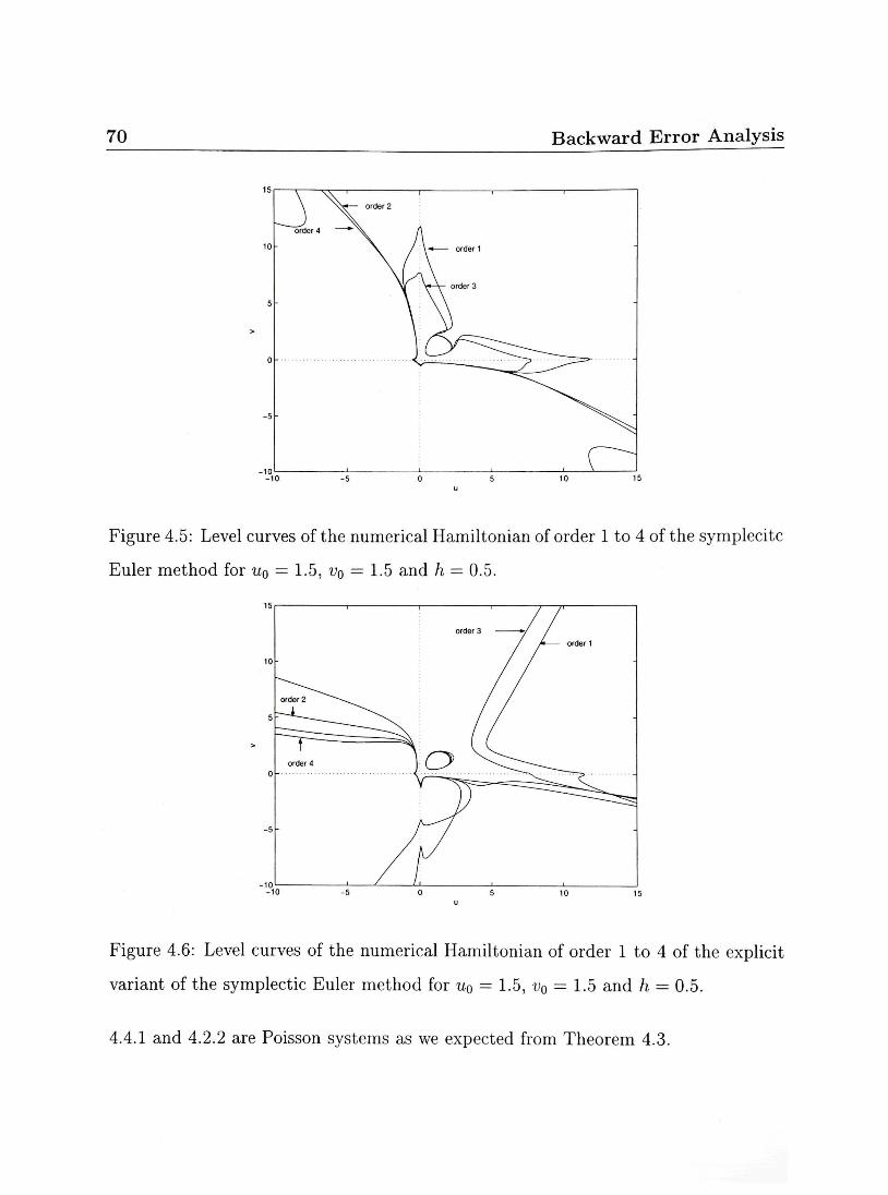
70 Backward Error Analysis
Figure 4.5: Level curves of the numerical Hamiltonian of order 1 to 4 of the symplecitc
Euler method for u0 = 1.5, vQ = 1.5 and h = 0.5.
10--
order 2 ^ " " - - ^ ^ ^
• — • — . ^ - v
order 4 ]
J
order 3
o ^
order 1
-
Figure 4.6: Level curves of the numerical Hamiltonian of order 1 to 4 of the explicit
variant of the symplectic Euler method for u0 = 1.5, VQ = 1.5 and h = 0.5.
4.4.1 and 4.2.2 are Poisson systems as we expected from Theorem 4.3.
71
Chapter 5
Exploitation of the Numerical
Hamiltonian
The aim of this chapter is to study the positivity of the numerical results given by
the explicit variant of the symplectic Euler method (EVSE) using backward error
analysis.
We mostly follow Sections IX.7 and IX.8 of [5] where the study focuses on Hamil
tonian systems. Some modifications are necessary to take into account the fact that
the Lotka-Volterra system is not a Hamiltonian but a Poisson system. We also trans
form some general results into ones more specific to EVSE in order to achieve better
bounds.
The procedure is to bound the local error of the numerical result and to use
this result and properties of Hamiltonian systems to bound the Hamiltonian error
\H{yn) — H{yo)\. This bound allows us to state our main theorem : given initial
conditions, we can compute for which step-size values the numerical solution given by
EVSE is ensured to remain positive over exponentially long time intervals. We also
give the procedure to find these step-sizes and illustrate it by a numerical example.
72 Exploitation of the Numerical Hamiltonian
5.1 Estimation of the Numerical Solution
We consider the Lotka-Volterra system
u = u (6 — v),
v = v (u — a),
which is a Poisson system whose Hamiltonian
H(u,v) = u - a lnu + v — b\nv
is analytic on E x E, where E := C\ {z \ Re(z) < 0 and Im(z) = 0} . We shall denote
for the rest of the chapter y := (u,v) and f{y) = (u(b - v),v{u - a))T. We apply
to the system the explicit variant of the symplectic Euler method $/i(y), defined by
(2.3), with step size h.
We fix a compact set K C D = {(u, v) G K2 | u > 0, v > 0} and define
i?:= a distance^, ESf),
where 0 < a < 1 can be arbitrarily chosen (we usually obtain better results if a is
large), so that for all u0 G K and all y such that \\y - y0\\ < R, y belongs to D.
Denoting by K the compact set K := { y | 3y0 € K such that ||y - y0|| < R} and by
M the bound M :— max{/(u,u) : (u,v) G K}, we now have, for all y0 G K,
\\f(y)\\<M for \\y-yo\\<R. (5.1)
As we saw in Section 4.4.1, we can write the explicit variant of the symplectic
Euler method applied to the Lotka-Volterra system as
$h{y)=y + hf{y) + h2d2(y), (5.2)
where d2{y) = (0,uv{b — v))T is analytic. Since we have to bound d2(y) for y G K,
we simply define M2 :— max{ut>(6 - v) : (u,v) G K} so that for all y0 G K,
\\d2{y)\\ = \uv{b - v)\ < M2 for \\y - y0|| < R. (5.3)
5.2 Estimation of the Coefficients of the Modified Equation 73
5.2 Estimation of the Coefficients of the Modified
Equation
Our task is now to bound the functions fd of the modified equation
ti = f(y) + hf2{y) + h2f3(y) + .... (5.4)
In order to simplify formulas, we may often denote / by f\. The key idea to obtain
an explicit formula for these functions, is to introduce the Lie derivative
[kb * d
D^Zfnv) dyW k
where y'fc' denotes the kth component of the vector y; in particular, for any differen-
tiable function g,
Djg(y) = g'{y)fj{y).
Using Lie derivatives and denoting y := y(t), we can write the solution of the
modified equation (5.4) expanded into a Taylor series as
y{t + h) = y + h{f{y) + hf2{y) + h2f3{y) + ...)
+ y(f'(y) + hf'M + .. -)(/(y) + hf2{y) + ...) + ...
= y + hf{y) + h2[f2(y) + ^f'f(y)}
+ h3[fM + ^(/2/(y) + f'f2(y)) + ^ ( /77(y) + /"//(?/))] + . . .
= y + hf{y) + h2[f2{y) + ^{Dlf1){y)]
+ h3[h{y) + y (D1/2 + D2fx){y) + ^{D2h){y)\ + ....
In other words, the solution of the modified equation (5.4), with initial value y{t) = y
can be formally written as
y{t + h)=y + J2^D^F{y), i>l
74 Exploitation of the Numerical Hamiltonian
where F(y) = fx{y) + hf2{y) + h2f3{y) + ... stands for the modified equation, and
hD = hDi + h2D2 + h3D3 + . . . for the corresponding Lie operator.
Expanding the formal sum, we obtain
y{t + h) = y + Y,x< (5.5) J2 hk^-+k'{Dkl...Dk^fki)(y) i>l " Ui, . . . ,ki
where all km > 1, and then we can compare like powers of h in the numerical method
(5.2) and the expansion of the exact solution (5.5) to obtain for j > 3,
2-^ j\ £ {Dkl...Dkx_Jki)(y) ki-\ \-ki=j
= 0
and for j = 2
In other words,
and
L^i\ i > l
] T (Dkl...Dki_1fkl)(y) .fci+-+fci=2
f2{y) = d2{y)-1-{D1f1){y)
= My)-
(5.6)
My) = -t1n Y, {Dkl...Dki_Jkl){y) , (5.7) »=2 " lki + -+k{=j
for j > 3, so if we want to get bounds for ||/j(y)||, we have to estimate first ||(Z>,a)(y)||
and for this we use the following variant of Cauchy's estimate given in [5].
Lemma 5.1. For analytic functions fj{y) and g(y) we have for 0 < a < p the
estimate
lAylU < p-a
11/tlU • h\\p-
Here, \\g\\p := max { \\g(y)\\ : y G Bp{y0)} and \\fi\\a, ||Ay||«7 are defined similarly.
Proof. Fix y G Bo(y0) and consider a(z) := g(y + zfr{y)). This function is analytic
for \z\ <£:= ^f with M := \\fi\\a. We then have
<*'(0)=9'(y)Mv) = (Dig)(y),
5.2 Estimation of the Coefficients of the Modified Equation 75
so applying Cauchy's estimate to a we obtain
ll(Ay)(y)|| = ||a'(0)|| < - sup ||a(z)|| = — M l , £ \Z\<E p-°~
and finally
|Ay|| < II/IIUIPIU p-a
D
The following theorem gives an explicit bound for the functions fj{y), for y G
K2 := {y | 3y0 G K s.t. \\y — y0|| < R/2 }. Note that this bound is only valid when
we apply the explicit variant of the symplectic Euler method to the Lotka-Volterra
system.
Theorem 5.1. For all yo G K, f{y) and the coefficients fj{y) of the modified dif
ferential equation (5.4) are analytic in Bn{yo), so if the bounds (5.1) and (5.3) are
satisfied, we have for the coefficients fj, j > 2,
11/)11 ^ ^ P ^ y - 1 for ytK2, (5.8)
where n := 2/(2 In 2 - 1) + M2R/M2.
Proof. We fix an index J > 1 and we want to bound | | / J | |H/2 = max{ ||/j(y)|| : y &
BR/2{yo)}. The trick of the proof is to introduce S := R/(2{J — 1)) and estimate
||/j|U-y-i)o, so that for j = J, we obtain | | / J | U - ( J - I ) * = II /JIU/2-
In order to simplify notations, we abbreviate || • ||fl_(j_i)5 by || • \\j. Applying
repeatedly Cauchy's estimate given in Lemma 5.1, we obtain for ki + \- hi = j ,
\\DklDk2. ..Dk%_Jki\\3 < i | | / f c l | | , • \\Dk2. ..Dki_Jki\\3_x
< T^IIAillj • l l / ^ l l i - l " \\Dkz • • • -Dfci-i/fcilli-2
< . . .
- Tizrll/fcillj' ll/^llj-i • ••• • ll/fci-illj-t+2• ll/fcj|j-i+i-
76 Exploitation of the Numerical Hamiltonian
By definition, for k < j we have BR_^_X)5 C BR^k^i)5, so that ||y||j < ||y||fc, so from
k\, k2,..., ki < j — i + 1, we obtain
\\DklDk2 . . . Dki_Jki\\j < ^ - H / f c J I f c ! -Il/fcjllifca • • • • • ll/fc-illfc.-i • WfkiWkr
We now apply this inequality to the expansions of the functions f3 given by (5.6) and
(5.7) and obtain
II/2H2 < ||d2||2 + i||I>l/l||2 < |M 2 | | 2 +-^ | | / l | | 2
and
Wf3(y)\\3<ztl E WD^.-.D^MIJ
i=2 ' ki + -+ki=j
3 1 1 ^ E " 7 ! E TiTlll/fcilUi • Il/fc2||fc2 ••••• H/fcJk-
i=2 ' ki+-+ki=j
We define, by induction,
V ' i=2 ki + -+ki=j
so that \\fj\\j < (3j6, for 1 < j < J, and we consider the generating function
&(0 = 5><J'
= E y ( ^ f V + E E * E A./V-.A.C j > l V 7 j>2 i=2 fci+-+fct=j
Denoting by 7 := M/5 and q := M2/M and assuming |g£| < 1 we obtain
6(0 = ^ + ^ - 6 ( 0 - 1 .
5.2 Estimation of the Coefficients of the Modified Equation 77
So denoting by y := 6(0, we have to solve
$ ( C , y ) : = e ^ - 2 y - l + - ^ - = 0 (5.9)
1 -q(
and since d$/dy = ey - 2, we can apply the implicit function theorem whenever
ey _ e6(c) ^ 2. We have ey = 2 for y = B : = In 2 + 2km, so we need
e6(c) - 26(0 = 1 1^7 / 2 - IB.
Solving this last equation we obtain that
2 5 - 1 c/ 7 + 9(25-1)
So finally 6(C) is analytic in a disc with radius £ := ^^ln^-i) centered at the origin.
One can note that since \ < -, the sum Ylj>o(lO'' m the derivation of 6(C) is well
defined.
Now we want to prove that on the disc |C| < £, the solution 6(C) of (5.9) with
6(0) = 0 is bounded by In 2. We consider first the map defined by w = j z ^ = \~TTZ~
and decompose it. The image of the disc |C| < \ under the mapping C •-> \ is the
disc |C| < v, then we apply the translation C >-+ C — Q a n d w e obtain the disc of radius
v centered at —q. Applying again the transformation ( H + ^ we obtain the disc of
radius , 2 V2| centered at Xj^ if Q ¥" v (which is always the case since 7 cannot be
zero). Finally we multiply by (—7) and obtain the disc centered at 2 ^ 2 and of radius
, 2^21 • Since v > q, the centre of the disc is negative and the largest point of the disc
is
w =— 2+—2 2 = = - 2 1 n 2 - l ) . ql — vl ql — vl q — v
So now we have to consider the image of the disc |UJ| < 2 In 2 — 1 centered at the origin
under the mapping 6(u>) defined by eb - 1 — 26 = w and 6(0) = 0. One can prove (see,
for example, [5] page 309) that it is completely contained in the disc |6| < In 2.
78 Exploitation of the Numerical Hamiltonian
Applying Cauchy's estimate to 6(C) = ]C7>1 PjC3\ we now obtain
\h 6^(0)
J! < In 2 v3
and thus | |/j |U/2 = \\fj\\j < 5/3j < In2 6 v3. By definition of v, we have
v = q + 7 M2
+ M M2 2M{J - 1)
2 1 n 2 - l M <5(21n2-l) M i ? (21n2- l )
M ( J - l ) R
2 RM2
+ 2 1 n 2 - l M 2 ( J - 1 ) , <
M ( J - l ) R
2 RM2
2 1 n 2 - l M2
so defining n := 2/(2 In 2 - 1) + RM2/M2, we obtain
v < M{J - l)n
R '
On the other hand, we have
5u = R R M(J - l)n
-v < 2(J-1) ~ 2 ( J - 1 ) R
Mn
so that finally, for J > 1, we obtain
11,11 ^ i «Mn (M{J-l)y \\fj\\R/2 < In2 — I
j - i
D
5.3 Estimation of the Local Error
As we said in Chapter 4, the modified differential equation series usually diverges, so
that we have to work with a truncated equation
y = FN(y), FN(y) = f(y) + hf2(y) + ••• + hN~lfN{y) (5.10)
5.3 Estimation of the Local Error 79
with initial value yo = yo- Supposing that hN < h0 with h0 := -^ and using the
bound (5.8), we estimate for y G K2,
\\FN(v)\\ = \\f(y) + Wv) + ••• + hN-]fN{y)\\
<\\f\\+h\\f2\\ + --- + hN-1\\fN\\ N
», V - , nvM (r]M{j-l)h\3'x
< M + 2 j ln2-y- I - v ' ' 3=2 ^
R
< M
< M
1 + In2 ^-J fnMjh0\
3
^ ^ E ^ - R A T J J=I
j = i v J
and since the sum in the last line is maximal for N = 2 and bounded by 0.184, we
obtain
\\FN{y)\\<M 1 + 1.0022 n-ln2
< M [1 + 0.06477] (5.11)
This estimation allows us to bound the local error.
Theorem 5.2. If h < ho/3 with ho = R/{enM), then there exists N = N(h) (namely
N equal to the largest integer satisfying hN < h0) such that, for any y0 G K, the
difference between the numerical solution yx = $n{yo) and the exact solution cf)^<t{yo)
of the truncated modified equation (5.10) satisfies
\\$h(yo) ~ 4>N,h{yo)\\ < h^/Me-^,
where 7 = e(2 + eJf^ + 0.064/7) .
Proof. For any yo G K fixed, we consider the function
g{h) := $h{yQ) - < ^ ( y 0 ) ,
which is analytic, since $n{yo) = yo + hf{y0) + h2d2{y0) and <j>Nth in Section 4.5 are
both analytic functions of h.
80 Exploitation of the Numerical Hamiltonian
By definition of the functions f3{y) of the modified equation, the coefficients of
the Taylor series for $h(yo) and cf>Nth are the same up to the hN-term, but not further
due to the truncation of the modified equation. Hence the function g(h) contains the
factor hN+1 and we can apply the maximum principle for analytic functions to -^r+r-
If g{z) is analytic for |z| < e, we have for 0 < h < e,
9(h) hN+l - 777+T m ^ x l ^^ £N+1 \z\<e
(5.12)
Since g{h) is analytic for any h, we can choose e = eho/N.
On the other hand we have
ll*z(l/o) - Vo\\ = \\zf(y0) + z2d2(y0)\\ < \z\M + \z\2M2.
Moreover ||F/v(y)|| < M(l + O.O6477) is valid for any y G K2 and any \h\ < e, so we
have
UNM) - yoll = \\y{z) - y(0)|| < \z\ • \\y{z)\\ = \z\ • \\FN{y)\\ < \z\M{l + 0.0647?),
as long as cj)N,z(yo) = y(z) stays in K2. In fact, because
eM(l + 0.06477) = ^ M ( l + 0.0647?) = ^-{- + 0.064) < y
since 77 > 5 and N > 3, the solution cj>N,z stays in the ball BR/2{y0) c K2 for all
\z\<e.
Finally we go back to (5.12). Since
| | ^ ) | | < | | ^ ( y 0 ) - yoll + MNAVO) - i/oll
< \z\M + \z\2M2 + M\z\{l + 0.0647?)
M, < \z\M (1 + \z\-j + 1 + 0.064/?),

5.4 Estimates of the Variation of the Hamiltonian 81
we have
\g(h)\\ < hN+l
—rrrr rnax £N+1 \z\<e
<
<
'/V
'/V
N+1
Mo \z\M (2 + \z\jf + 0.064/?)
Mo eM (2 + e-j- + 0.064T?)
M N
hM 2 + ^ + 0 . 0 6 4 7 ? '
W
<- £ J -NM
2 + ^ + 0 . 0 ^
Then, because /W < /io, we obtain
e/ln
iV
< e -N
and
|y(/i)|| < e~NhM 2 + ^ + o.oa4,
Finally, since iV < h0/h < N + 1, we have e /l0/'/l > e (Ar+1) and the theorem is
proved.
•
5.4 Estimates of the Variation of the Hamiltonian
We are now in a position to prove that if the numerical result stays in a compact set,
then it is really close to the exact trajectory for exponentially long time intervals.
Theorem 5.3. / / the numerical solution stays in the compact set K2 C D = {u >
0,v > 0} and if h < h0/3, with h0 = R/{enM), then there exist N = N{h) (the
largest integer satisfying hN < ho) such that, over exponentially long time intervals
nh < eho/2h,
\H{yn)-H{yo)\<L1Me-h°/2h
(5.13) \H(yn) - H{y0)\ < L jMe^2*1 + 2hC
82 Exploitation of the Numerical Hamiltonian
with L := M ( 1 + 0 . 0 6 4 T ? ) and C : = 0 .277MV (u„ i„ -R/2) ( i ; m i n - f l /2 ) »•<"* ^ — (umxn-R/2)(vmln-R/2)-
(u, u) G K} and vmm is defined in a similar way.
where umin := min{ u :
Proof. Let 0Arjt(yo) be the flow of the truncated modified equation (5.4). As stated
in Theorem 4.3, this differential equation is a Poisson system whose Hamiltonian is
H = H + hH2 + h2H3 + ••• + hN~lHN, so that
H{4>Ntt{yo))=H{y0), Vt.
Our first goal is to bound VH. By definition of Poisson systems, we have
FN(y) = /(!/) + hf2{y) + ••• + hN~lfN{y) = B{y)VH{y),
and using the bound on ||F/v(y)|| derived in (5.11), we have
\\B{y)VH{y)\\< M(l + 0.064T?).
On the other hand, since we consider the Lotka-Volterra system, we have
so that
\B(v)VH(y)\\ =
6 < M(l+0.064,) K
uvHv(y)
-uvHu(y) = \uv\
Hv(y)
-Hu(y) = \uv\ \\VH{y)\\
M(l + 0.064T?) = :L,
\uv\ (umin - R/2){vmin - R/2)
since min{ u : (u, v) G K2} — um,n — R/2 and similarly for v. The bound L is in fact
a global /Vindependent Lipschitz constant for H and
||tf (yn+1) - H{4)N,h{yn))\\ < L \\yn+1 - 4>N,h{yn)\\ < L hjMe-h°/h,
by Theorem 5.2.
We are now in a position to bound
\H(yn)-H(yo)\ = n n
] T [H{yj) - Hiy^)] = ] T [H(yj) - H{^h{y3-i)) 3=1 j = l 3 = 1 n
<Y^\L hjMe-ko/h\ = nhL -yMe-ho/h,
5.4 Estimates of the Variation of the Hamiltonian 83
so that for nh < eh°/2h, we have
\H{yn)-H{yo)\<L1Me-h°/2h,
which is the first inequality we wanted to prove.
It remains to show an equivalent result for the Hamiltonian. Since
H(y) = H{y) + h[H2{y) + hH3(y) + ••• + hN~2HN{y)},
we have to prove that H2{y) + hH3{y) -I \- hN~2HN{y) is uniformly bounded on
K independently of h and N. By Theorem 4.3, we have for all j
fj(y) = B(y)9j(y) = B{y)VH3(y),
so that, using the bound (5.8), we have for j > 2 and y G K2
\\f3{y)\\ = \uv\ • \\VH3{y)\\ = \uv\ • ||0j(y)|| < In2 ^ (vM{jR
lY
On the other hand, the proof of the Integrability Lemma 4.1 gives
Hj(y) = (y- zo)Tgj(z0 + t(y - z0))dt Jo
for any ZQ G K. So we can choose z0 such that ||y — z0\\ < R/2 and then
WHMW = II / (9 ~ zo)T93(zo + t{y - zQ))dt \\ Jo
< [ \\(y-zo)\\-\\gj(zo+t{y-zo))\\dt Jo
3-1
J - l R 1 \n2Mrj (nM{j -1)'
~ ~2~]u~v\ 2 V P /
JUn2M7? fnM{j-l)\j-1
~ 4{umin-R/2){vmin-R/2) { R )
84 Exploitation of the Numerical Hamiltonian
and then
\\H2(y) + hH3{y) + ---+hN-2HN{y)\\
< A R\n2Mn fnM{j-l)\]-1 h
~ h 4(u™- - ^/2)(«min - R/2) \ R J
^ R\n2Mn fnMhj\3~l nMj ~ f^ 4(umin- R/2){vmm- R/2) V R ) R
< ln2MV ^ . (j_\-1
~ 4(umin - R/2){vmin - R/2) jx[3\eN)
< ^ V -YeNf-LY ~ 4(umin - R/2){vmin - R/2) frt \eNj '
^;v-l and since the sum Ylj=i ^(^v)3 is maximal for N = 4 and is bounded by 0.588 we
define
0.588 e In 2M2T?2 _ 0.277MV ' " 4(umin - R/2)(vmin - R/2) ~ (umin - R/2){vm[n - R/2)
and H2{y) + hH3{y) + • • • + hN~2HN{y) is uniformly bounded on K by C. Finally we
have for nh < eho/2h
\H(yn)-H(yo)\ < L^Me-^2h+ 2hC.
•
5.5 Application
We can apply Theorem 5.3 to our problem, namely "how to be sure that the method
remains positive". The constructive proof of the following theorem gives a routine
which enables us to determine the step-size h* for which the numerical result stays in
the first quadrant over exponentially long time intervals.
5.5 Application 85
Theorem 5.4. Let (u0,v0) be given initial conditions, and let h* be the minimum of
ho/3 and the unique solution of
L1Me~h^2h + 2hC = Hmax- H0,
where the constants h0,L,j,M,C,Hm:ix and H0 are defined in the proof below. Then if
we apply the explicit variant of the symplectic Euler method with a step-size h smaller
than h*, the numerical solution stays positive over exponentially long time intervals
t = nh* < eh°l2h*.
Proof. The constants a, 6, u0 and u0 are fixed, so that we can compute
HQ :— H{u0, v0) — u0 - a In u0 + v0 - 6 In v0.
The level curve of H0 defines the compact set K. Then we compute the maximum
values and the minimum values of u and v in K and we obtain the values of
«max :=max{u : (u, v) G K},
Umin :=min{u : (u, v) G K},
^max :=max{u : {u,v) G K),
^min := min {v : (u, v) G K}.
Then we set R := a min{ umjn, vmin } with, for example, a = 9/10, so that we can
define the compact set K — { y : 3 y0 G K such that ||y - y0|| < R} and in a similar
way, K2.
We have by definition M := max{/(u, v) \ {u,v) G K}, however it is much easier
to use
M = max { umax(i;max - 6), wmax(umax -a)}
where umax = max{u | (u, v) G K} = umax + R and umax = umax + R. Similarly we use
M2 = umaxtjmax(umax - 6)
86 Exploitation of the Numerical Hamiltonian
instead of max e^ ||d2(y)||.
Once we have these values, we can compute
2 RM2 , , R 7? = 1 — and ho — 2 In 2 - 1 M2 enM
as well as 7 = e[2 + ^ ^ + 0.064/?],
- _ M(l + 0.064/?) ~ {umin-R/2)(vmm-R/2)
and _ 0.277M2/?2
{umin-R/2){vmin-R/2)
The next step is to choose h smaller than h0/3. Once h is chosen, we check
whether or not it is small enough to ensure that the numerical solution stays in K2.
We know that the bound (5.13) is valid if and only if yn is in K2, so we need to know
that it does stay in this compact set.
Defining Hma.x := min{H{u,v)\{u,v) G dK2} = m'm{ H{umm-R/2, b),H(a, vmin-
R/2) }, we know that yn stays in K2, if
H(yn) - Ho < //max - Ho
that is, using the bound (5.13), if
L 1Me-hol2h + 2hC < tfmax - H0. (5.14)
Now all the constants in the above expression are positive, and since any function
of the form
f{h) = ae-ho/2k + (3h-6
where a, /3, and 6 are positive, is strictly increasing, h satisfies inequality (5.14) if
and only if h is smaller than the unique solution of
L ^Me-ho/2k + 2hC = # m a x - HQ. (5.15)
5.6 Example 87
In other words, the bound h* we are looking for is given by the minimum of h0/3
and the solution of (5.15). Moreover, the numerical solution stays in K2 for at least
t = nh*< ehol2h'.
•
5.6 Example
As an illustration, we consider the problem
u = u (1 — v),
i) — v (u — 2),
with the initial condition u(0) = 1.5, v{0) = 0.5.
The exact solution of the system stays on the level curve of the Hamiltonian
with H0 = 1.8822, so we define K = {{u,v) | \H{u,v)\ < 1.8822} and then umin =
1.135, umax = 3.222,vmin = 0.4343 and ?jmax = 1.921. We obtain R = 0.3909 and we
compute h0 — 0.0057, so we have to choose h to be smaller than h0/3 = 0.0019. Since
the solution of
L 1Me-h°'2h + 2hC = # m a x - Ho
is 0.000113, we conclude that for values of h smaller that 0.000113, we are sure that
the numerical Hamiltonian is well-conserved and that the numerical solution stays
positive and exhibits the right qualitative behaviour, for a time t = nh ~ 1015.
It is interesting to note that, as one can see on Figure 5.1, the estimate for h is
really pessimistic. For values as large as h = 0.1, the Hamiltonian is extremely well-
conserved, with maxn>i \H{yn) - H0\ = 0.0127 and the numerical simulation starts
to leave the first quadrant for values of h greater or equal to 0.7.
An important remark is that we not only proved that the numerical solution of
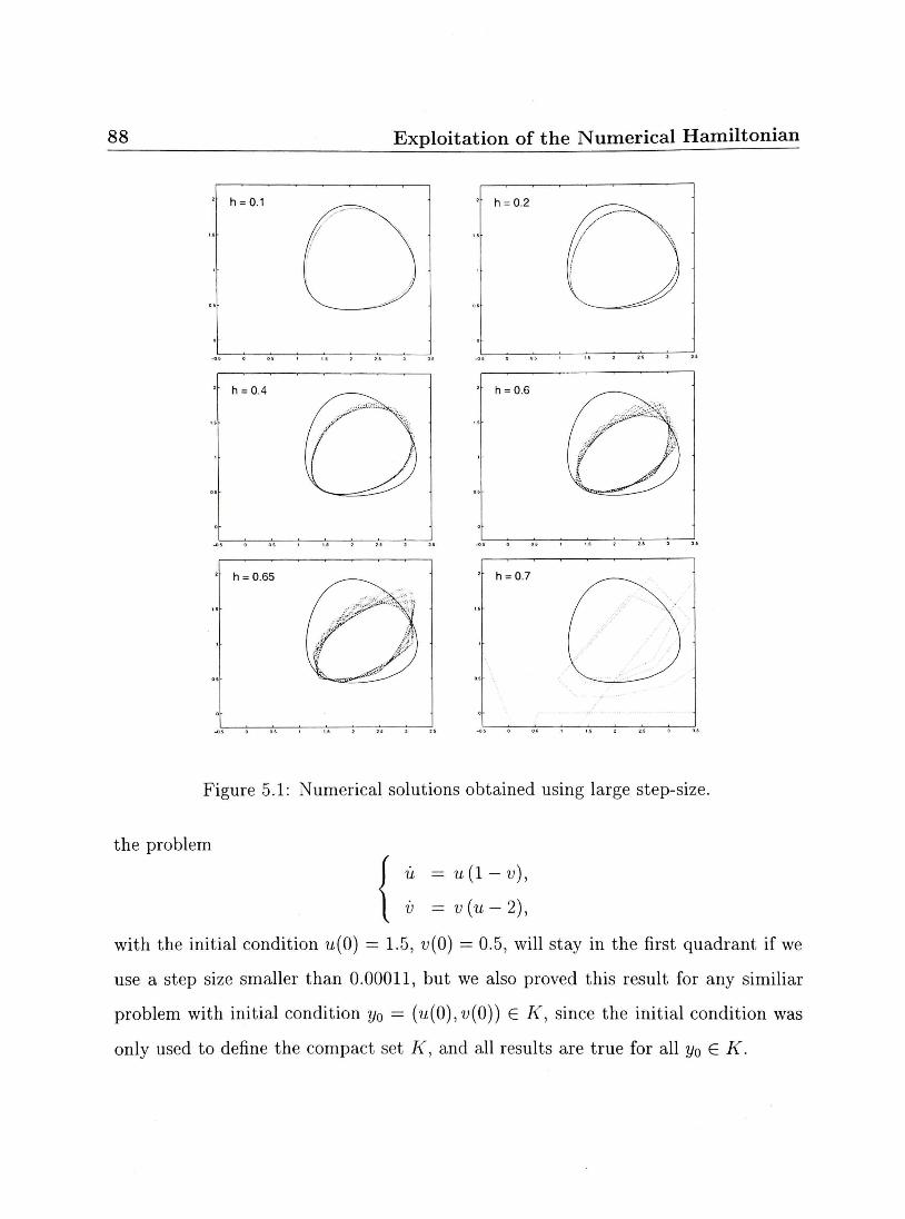
88 Exploitation of the Numerical Hamiltonian
h = 0.2
•
/ [1
X
n
-
Figure 5.1: Numerical solutions obtained using large step-size.
the problem
ii = u (1 — v),
v = v (u — 2),
with the initial condition u(0) = 1.5, v{0) — 0.5, will stay in the first quadrant if we
use a step size smaller than 0.00011, but we also proved this result for any similiar
problem with initial condition y0 = (u(0),w(0)) G A', since the initial condition was
only used to define the compact set K, and all results are true for all yo G K.
89
Conclusion
In this thesis we mostly focused on two properties of the Lotka-Volterra system: its
cyclicity, by the mean of its Poisson structure, and its positivity. As we pointed out
in the introduction, geometric integration has been studying, among other topics,
numerical methods preserving Poisson structure. Independently of geometric inte
gration, there is current research focusing on the positivity of numerical methods.
Our goal was to unify these two subjects. We first studied the symplecticity of the
symplectic Euler method and its explicit variant and then we proved that they are
Poisson integrators for the Lotka-Volterra system. The latter property explains their
excellent performance in general. We finally focused on the positivity of the numerical
results.
In the case of the Lotka-Volterra system, we derived simple conditions ensuring
the positivity of the symplectic Euler method, whereas we should expect from Figure
2.9 which gives the number of iterations needed for each point to leave the first
quadrant, that those conditions are not as simple for its explicit variant (2.3). To
study these conditions, we used backward error analysis, but this analysis needed
to be more refined than what is generally required. Since this concept is usually
employed to study the qualitative behaviour of numerical methods over long time
intervals, the idea is in general to prove that the order of the error is small. However
for our problem, we needed precise bounds on the error, in Theorem 5.3 in particular,
in order to ensure the positivity of the numerical results. The last chapter is an
90 Conclusion
excellent illustration of a concrete application of backward error analysis for Poisson
systems.
These results are, of course, very restricted as they are only valid for the symplectic
Euler method and its variant when they are applied to the Lotka-Volterra system.
However, nothing proves that it will not be possible to first generalize the results
and the procedure given in Chapter 5 for the explicit variant of the symplectic Euler
method applied to any Poisson system and then to find similar results for other
methods.
We observed, in particular, that several second-order methods, such as the implicit
midpoint rule, the trapezoidal rule and the Stormer-Verlet method, exhibit the same
characteristics as the explicit variant of the symplectic Euler method. Even if, in
general, the numerical approximations show the correct qualitative behaviour, they
may become negative depending on the choice of the initial conditions and step size.
By plotting the number of iterations needed for each point to leave the first quadrant
when we apply one of these three methods to the Lotka-Volterra system with h = 1,
we notice on Figures 5.2, 5.3 and 5.4 that we get trajectories leaving the first quadrant.
For the implicit midpoint rule and the trapezoidal rule, the region consisting of
initial values for which the numerical result is positive for 100 iterations is large
(almost [0,3] x [0.3]), whereas the one corresponding to the Stormer-Verlet method
is much smaller and similar to the one corresponding to the explicit variant of the
symplectic Euler method (see Figure 2.9). Using the tools we derived in this thesis,
it should be possible to give conditions on the step size to ensure the positivity of the
numerical approximations over long time intervals. One could start by the Stormer-
Verlet method as it is a Poisson integrator for the Lotka-Volterra system. Then the
results could be generalized to the implicit midpoint rule, which is symplectic but
not a Poisson integrator. Finally one could study the case of the trapezoidal rule.
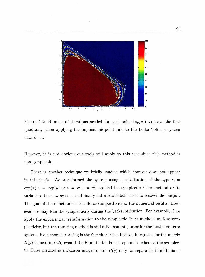
91
Figure 5.2: Number of iterations needed for each point (u0,i>o) to leave the first
quadrant, when applying the implicit midpoint rule to the Lotka-Volterra system
with h = 1.
However, it is not obvious our tools still apply to this case since this method is
non-symplectic.
There is another technique we briefly studied which however does not appear
in this thesis. We transformed the system using a substitution of the type u =
exp{x),v = exp(y) or u = x2,v = y2, applied the symplectic Euler method or its
variant to the new system, and finally did a backsubstitution to recover the output.
The goal of these methods is to enforce the positivity of the numerical results. How
ever, we may lose the symplecticity during the backsubstitution. For example, if we
apply the exponential transformation to the symplectic Euler method, we lose sym
plecticity, but the resulting method is still a Poisson integrator for the Lotka-Volterra
system. Even more surprising is the fact that it is a Poisson integrator for the matrix
B(y) defined in (3.5) even if the Hamiltonian is not separable, whereas the symplec
tic Euler method is a Poisson integrator for B{y) only for separable Hamiltonians.
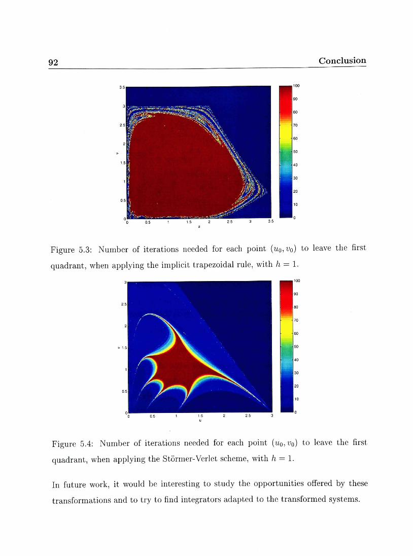
92 Conclusion
Figure 5.3: Number of iterations needed for each point {u0,v0) to leave the first
quadrant, when applying the implicit trapezoidal rule, with h = 1.
Figure 5.4: Number of iterations needed for each point (IIQ,V0) to leave the first
quadrant, when applying the Stormer-Verlet scheme, with h = l.
In future work, it would be interesting to study the opportunities offered by these
transformations and to try to find integrators adapted to the transformed systems.
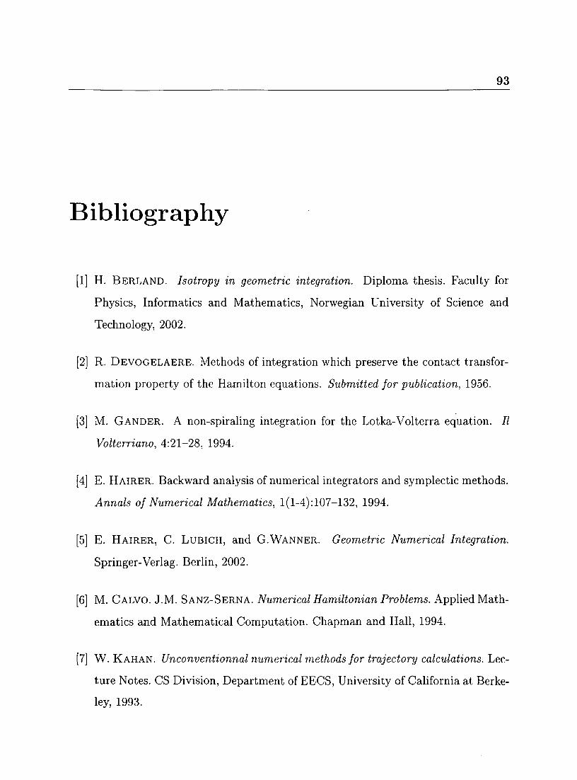
93
Bibliography
[1] H. BERLAND. Isotropy in geometric integration. Diploma thesis. Faculty for
Physics, Informatics and Mathematics, Norwegian University of Science and
Technology, 2002.
[2] R. DEVOGELAERE. Methods of integration which preserve the contact transfor
mation property of the Hamilton equations. Submitted for publication, 1956.
[3] M. GANDER. A non-spiraling integration for the Lotka-Volterra equation. II
Volterriano, 4:21-28, 1994.
[4] E. HAIRER. Backward analysis of numerical integrators and symplectic methods.
Annals of Numerical Mathematics, 1(1-4):107-132, 1994.
[5] E. HAIRER, C. LUBICH, and G.WANNER. Geometric Numerical Integration.
Springer-Verlag. Berlin, 2002.
[6] M. CALVO. J.M. SANZ-SERNA. Numerical Hamiltonian Problems. Applied Math
ematics and Mathematical Computation. Chapman and Hall, 1994.
[7] W. KAHAN. Unconventionnal numerical methods for trajectory calculations. Lec
ture Notes. CS Division, Department of EECS, University of California at Berke
ley, 1993.
94 BIBLIOGRAPHY
[8] R. MEYER-SPASCHE. M.J. GANDER. An introduction to numerical integrators
preserving physical properties. In Applications of Nonstandard Finite Difference
Schemes, pages 1-67. 2000.
[9] J. SANZ-SERNA. An unconventionnal symplectic integrator of W. Kahan. Tech
nical report, Universidad de Valladolid, Spain, 1994. Report 1994/2.
[10] J. STURGEON and B. LAIRD. Symplectic algorithm for constant-pressure molec
ular dynamics using a Nose-Poincare thermostat. Journal of Chemical Physics,
112(8):3474-82, 2000.
[11] P. TUPPER. Topics in the Numerical Analysis of Ordinary Differential Equations:
Molecular Dynamics and Chemical Kinetics. PhD thesis, Scientific Computing-
Computational Mathematics Program, Stanford University, 2002.

![Competitive Lotka-Volterra Population Dynamics with · PDF filearXiv:1102.2163v1 [math.PR] 10 Feb 2011 Competitive Lotka-Volterra Population Dynamics with Jumps Jianhai Bao1,3, Xuerong](https://img.pdfslide.us/doc/110x75/5aa5c9347f8b9a185d8dc6a8/competitive-lotka-volterra-population-dynamics-with-11022163v1-mathpr-10.jpg)