Embed Size (px)
Citation preview

1
Symmetry & Relations
In the proximal arteries of ischemic stroke patients
Symmetrical or not?
Bachelor thesis Physics and Astronomy, 12EC,
From 27 june 2013 – 11 oktober 2013
Author: Hilmar van der Veen (5743257)
Supervisor: MSc Emilie Santos (PhD student)
Second supervisor: Dr. Henk Marquering
Second examiner: Prof. Dr. Ton van Leeuwen

2
Samenvatting
Een beroerte is een plotselinge afname in de toevoer van zuurstofrijk bloed aan de hersen. Dit wordt
meestal veroorzaakt doordat een bloedprop of trombus een bloedvat in de hersenen afsluit. De
locatie van de trombus wordt bepaald middels een computed tomography angiography (CTA). Dit is
een methode waarbij met behulp van contrast vloeistof in combinatie met een CT-scan de
bloedvaten in de hersenen zichtbaar worden gemaakt.
Het bepalen van de locatie van de bloedprop alleen is niet voldoende om de patiënt direct de juiste
medicatie te geven. Hiertoe is ook de afmeting van de trombus van belang. Gedaan onderzoek wijst
uit dat de lengte van de trombus een grote rol speelt bij het succesvol kunnen rekanaliseren van het
bloedvat [9].
Nader onderzoek, aan het AMC en Erasmus MC, is gedaan naar het reconstrueren van een afgesloten
bloedvat. De toegepaste reconstructie methode is gebaseerd op de symmetrie van de bloedvaten in
de nabijheid van de cirkel van Willis.
Om gebruik te kunnen maken van symmetrie is het noodzakelijk dat de cirkel van Willis compleet is.
Slechts 29% van alle patiënten met een beroerte hebben een complete cirkel van Willis. Om ook in
gevallen van een niet complete cirkel van Willis de afmeting van de trombus te kunnen bepalen is het
raadzaam om meer inzicht te krijgen in de relaties van de bloedvaten onderling.
Binnen dit project wordt bepaald in welke mate de binnenste halsslagaders, de middelste en de
voorste hersenslagaders een significante correlatie vertonen; in hun lengte, mate van maximale
kromming, onderlinge hoeken, en onderlinge straal. Ook wordt er bepaald in hoe verre er sprake is
van symmetrie, waarbij de mate van symmetrie bepaald wordt in het geval van een volledige cirkel
van Willis.
Bij dit project zijn de sterk significante arteriële correlaties vooral gevonden in de onderlinge straal
van de bloedvaten en in de lengte van het bloedvat ten opzichte van zijn eigen maximale kromming.

3
Inhoud
Samenvatting ........................................................................................................................................... 2
Introduction ............................................................................................................................................. 5
1. Stroke .......................................................................................................................................... 5
2. Imaging ........................................................................................................................................ 5
2.1 CTA ....................................................................................................................................... 5
2.2 Baseline and Follow up CTA ................................................................................................ 5
3. Treatment ischemic stroke .......................................................................................................... 5
4. Current researches ...................................................................................................................... 6
5. Arteries ........................................................................................................................................ 7
5.1 Internal Carotid Artery ........................................................................................................ 7
5.2 The Middle Cerebral Artery ................................................................................................. 8
5.3 The anterior cerebral artery ................................................................................................ 8
5.4 The circle of Willis and its variants ...................................................................................... 8
Background and Purpose ........................................................................................................................ 9
Research questions: ............................................................................................................................ 9
Method .................................................................................................................................................... 9
1. Introduction ................................................................................................................................. 9
1.1 Software .............................................................................................................................. 9
1.2 Networks ............................................................................................................................. 9
2. Data ........................................................................................................................................... 10
3. Exclusion criteria ....................................................................................................................... 10
4. Segmentation ............................................................................................................................ 10
a. Marking.................................................................................................................................. 10
b. Minimum Cost path. .............................................................................................................. 11
c. Robust shape regression for supervised vessel segmentation. ............................................ 12
Measurement and statistical method ................................................................................................... 13
1. The vessel length and curvature ............................................................................................... 13
2. The angle ................................................................................................................................... 13
3. The radius .................................................................................................................................. 14
4. Pearson correlation coefficient ................................................................................................. 14
5. Paired T-test .............................................................................................................................. 14
Results ................................................................................................................................................... 15
Correlation and significance .......................................................................................................... 15
Paired T-test .................................................................................................................................. 15

4
Discussion .............................................................................................................................................. 16
Relations between the arteries ..................................................................................................... 16
Symmetry in the proximal arteries ................................................................................................ 16
Limitations ..................................................................................................................................... 16
Conclusion ............................................................................................................................................. 17
Epilogue ................................................................................................................................................. 17
References ............................................................................................................................................. 18
Appendix A ............................................................................................................................................ 19
Appendix B ............................................................................................................................................ 21
Appendix C............................................................................................................................................. 24
Appendix D ............................................................................................................................................ 25

5
Introduction
Stroke Stroke or cerebrovascular accident (CVA) is the sudden loss of oxygenated blood supply to the brain
due to a blockage (Ischemic) or an haemorrhage. The blockage is mostly caused by a thrombus or an
embolus in a vessel. An haemorrhagic stroke occurs when a vessel fractures and blood locally
streams into the brain tissue. In both cases a rapid decline in brain function occurs due to tissue
necrosis. Ischemic stroke happens most frequently with 87%, while haemorrhagia only occurs in 13%
of all cases.
Figure 1: Illustration “A” shows two causes for ischemic stroke to happen. The first cause is due to a blood clot or an embolus blocking the vessel. The second cause is due to stenosis of the artery, also called atherosclerosis. Illustration “B” shows the two type of stroke: Ischemic and Hemorrhagic. [Illustration A: (http://www.drugs.com/health-guide/transient-ischemic-attack-tia.html)].
[Illisutration B:(http://www.drugs.com/health-guide/transient-ischemic-attack-tia.html)
Imaging
2.1 CTA
Computed Tomography Angiography (CTA) is an imaging technique, based on computed
tomography, that visualize the vessels and map them into a 3D image. The visualisation of the
arteries is done by administering the patient with a contrast agent short before the scan takes place.
If a CTA scan is made of the brain of a stroke patients, occluded segments parts (vessel without
contrast) will reveal the thrombus location in the arteries.
2.2 Baseline and Follow up CTA
A baseline CTA is a scan performed before an intervention. A radiologist diagnoses the baseline CTA
and decides what type of treatment is going to be applied. However, baseline CTA images may also
be useful for scientific purposes. The follow up CTA scan is done after a recanalization procedure to
observe if the treatment was successful.
Treatment ischemic stroke Treatment of acute ischemic stroke aims for the reperfusion of the cerebral arteries. Two methods
are used: chemical or mechanical. Tissue plasminogen activator (tPA) is given to the patients in order
to dissolve the thrombus. Alternatively, if the tPA fails, intravenous treatment using a catheter, stent
or MERCI device is then used to remove the thrombus manually.

6
Figure 2: Illustration “A” and “B” show how the tissue plasminogen activator (tPA) dissolves the blood clot (or fibrin) and restores the blood flow. Illustration “C” shows the manual removal of the thrombus or embolus with a mechanical device. [Illustration A: (http://www.askdoctork.com/can-you-explain-how-tpa-works-to-treat-a-stroke-201308055223) ] [Illustration B: (http://www.zina-
studio.com/p447740290/hF59B5E7#hf59b5e7)].
Numerous studies have demonstrated that thrombus characteristics (its size, location, and density)
are related with treatment success. Thrombus characteristics are by consequent a potential predictor
of patient outcome. It is then important to collect this information when the ischemic stroke patient
is admitted to the hospital.
Current researches
Figure 3: Example of final 3D rendering of the lumen (in blue) and thrombus segmentation (in red). [Symmetry based computer aided segmentation of occluded cerebral arteries on CT Angiography, Emilie SANTOS]
The AMC in collaboration with Erasmus MC (Rotterdam) aims to develop an automatic thrombus
segmentation and characterization pipeline on CT angiography for analyses and admission
diagnostics. But, this task is challenging since the lack of contrast between low density thrombus and
surrounding brain tissue in CT images makes manual delineation a difficult, time consuming and
often impossible task. One of the solutions developed was to exploits the absence of contrast at the
site of thrombus by using anatomical information from the contralateral side of the brain. The
method is based on a shape prior generation from the segmentation of the contralateral artery,
mirror symmetry and local image intensity.

7
Figure 4: The healthy side is mirrored onto the occluded side. [vessel disease map, AMC]
Arteries
5.1 Internal Carotid Artery
The internal carotid artery (ICA) is one of the three main arteries supplying the brain of oxygenated
blood. This artery consists of seven segments, which are denoted by C1 - C7, and start in the middle
of the neck, where it branches from the common carotid artery. In Figure 3 a representation of the
internal carotid artery is shown.
Figure 2 This figure shows the regional segments of the ICA starting from C1 to C7. The left image is a coronal view of the internal carotid artery (ICA), middle cerebral artery (MCA) and anterior cerebral artery (ACA). The image at the right shows a sagittal view of these same arteries. [http://radiopaedia.org/images/25325]

8
5.2 The Middle Cerebral Artery
The middle cerebral artery (MCA) is divided into 4 segments and starts at the branching of the ICA.
The M1 segment, or horizontal segment, is the segmental part between the ICA and the bifurcation
at the Silvian fissure. The M2 segment is in 78% of the time bifurcated.
Figure 4: Five variations of the MCA are shown in illustrations A to E. However, 78% of all stroke patients have an M2 segment that is bifurcated. Only 12% of the patients have an M2 which is trifurcated and 10% have an M2 that is furcating into more trunks. The illustrations F and G give a full depiction of how the arteries the ICA, the ACA A1 and the MCA. [4]
5.3 The anterior cerebral artery
The anterior cerebral artery (ACA) supplies the middle part of the brain and is divided into 3
segments. The A1 segment is part of the Circle of Willis and connected to the ICA. The ACA is also
connected to the ACA of the other brain part by the anterior communicating artery (AcomA). In
Figure 4F both A1 and A2 segments are represented.
5.4 The circle of Willis and its variants
The circle of Willis is a system of connected arteries. This system is also responsible for the
distribution of oxygenated blood over the brain. However, its main purpose is to connect the internal
carotid and the vertebral artery. For the main reason, if one supplying artery fails the other is used as
collateral. It has been demonstrated in literature that the circle of Willis present normal variations as
shown in Figure 5.
Figure 5: Eleven variants of the Circle of Willis are shown. Only 29% of all stroke patients have a complete circle of Willis. The number in parenthesis quantify the occurrences. [6]

9
Background and Purpose
We saw that the circle of Willis have been reported not to be complete for 71% of the time. It is not
always possible to use mirror symmetry to reconstruct the occluded side by using vascular
information of the contralateral side, as hypothesized, by AMC researchers. Therefore, measuring
correlations between proximal arteries would allow researchers to determine linear models and
finally reconstruct the occluded vessel.
Moreover, to our knowledge there has never been any report of any study focused on the
measurements and the verifications of the partial or complete symmetry into full circle of wills.
Research questions: This study aims to answer the following questions:
In case of a complete artery tree, is perfect symmetry present?
Would it be possible to reconstruct missing segment of an artery using the local
vessel information?
Method
1. Introduction A large amount of segmented CTA images needs to be processed in order to obtain useful
measurements. Processing these segmentation manually is a long and sturdy job to do. Regarding
the limited time dedicated to this research project, it is necessary to limit manual annotations as
much as possible.
1.1 Software
To automated the segmentation and perform our measurements, an image processing software was
required. The entire image processing pipeline was then implemented in MeVisLab®. MeVisLab is an
open source software, available at http://www.mevislab.de. It is based on a modular framework for
the development of image processing algorithms for visualization and interaction methods.
MeVisLab includes advanced medical imaging algorithms for segmentation, registration, and
quantitative morphological and functional image analysis.
Libraries have been developed by research groups and contain more than 1000 preprogramed
modules in C++, java or python. Each module can be linked between each other, creating functional
modular networks.
1.2 Networks
A Robust kernel segmentation network is available at the AMC. The network will give a fully
segmented vessel as output. We decided to use it since it has been proven to be equivalent to
manual segmentation but perform much faster. The network works with the following input:
a curve going through the complete vessel, not necessarily a centerline.
background values.
a good quality CTA image

10
The generation of the curve line will also be automated using a Minimum Cost Path method. The cost
image is calculated from Frangi’s Vesselness filter to highlight the tubular shapes in the images. The
Skull may also be interpreted as a tubular shape by the filter. Therefore we need to mask the skull in
the CTA image before applying the vesselness filter.
Data In order to answer the research questions, we will use the CTA scans of the MR Clean patient
population. MR Clean is an abbreviation for multicenter randomized controlled clinical trial. Its aim is
to investigate the therapeutics value of endovascular treatment for stroke patient. It was started in
December 2010. Approximately 17 medical centers in the Netherlands participated to the inclusion.
The number of patients included is now 365.
Exclusion criteria An exclusion criteria is used to separate between usable and unusable CTA scans. This criteria reads
as follows:
The CTA needs to be of High quality,
The slice thickness is not more than 1mm.
High quality means that the CTA scan does not contain much aliasing artifacts or too much noise. At
least not in the region where the relevant arteries are located.
Segmentation
a. Marking
To define the initial and final points of the artery we manually have to place these two marker points
at the right location, like in figure 5. For placing the marker points at the same position in every CTA
scan the following rules are needed to be followed:
The first marking point A is placed in the ICA at the same level of the peak of the dens axis.
The second marking point B is placed in the branching of the ICA into the proximal M1 and
the proximal A1.
The third marking point C is placed at the branching of the proximal M1 into the two
proximal M2 trunks.
The fourth marking point D is placed at the first branching spot of the anterior M2 trunk
encountered towards the side of the brain.
The fifth marking point E is placed at the first branching spot of the superior M2 trunk
encountered towards the side of the brain
The sixth marking point F is placed at the end of the A1 segment of the ACA, where the
artery branches into the A2 segment and the anterior communicating artery (AcomA).
These marker points will be used as an input for both the minimum cost path and the measurement
of the angles.

11
Figure 5: The letters A, B, C, D, E, F are manually placed marker points and define the initial and final position of an artery’s segment.
b. Minimum Cost path.
The minimum cost path [1] determines the shortest path between two predefined marker points in
any cost image. For our study the cost image is defined from a CTA image whereupon a skull mask
image and a Vesselness filter is applied.
This combined image needs to be added by a small value to remove all the values equal to zero
before getting inversed. Otherwise singularity problems will arise. The resulting Cost image will be
used by the minimum cost path to generate the curve going through the artery between the two
previously placed marking points.
Figure 6: The minimum cost path creates a guided centerline between two manually placed marker points, defining the initial and final point of the relevant segment.

12
c. Robust shape regression for supervised vessel segmentation.
The robust shape regression for supervised vessel segmentation (RSRSVS) is built around the
following modules:
the lumen segmentation intensity probability (LSIP),
the radial graph cut (RGC),
and the radial distance regression (RDR).
A point marked on the vessel, as a reference, together with an earlier defined frame around it are
used as the input for the LSIP. The frame’s spatial dimension is 4,00x4,00x15,73 mm. The LSIP
normalizes the intensity in the given frame between 0 and 1. With the 0 value defined as the value of
the surrounding background intensity of the vessel.
The RGC uses this frame work to define the vessel’s boundary and redefines the existing values into
binary values. Where the zero value defines the outside of the vessel whereas the value 1 defines the
inside. The output of the RGC is an uniform valued slab, shown in figure 7.
The RDR smoothens the contour to obtain a more circle like image. The RDR gives only the smoothed
contour as an output. This smoothed contour is also known as a contour segmented object (CSO)
Figure 7: The Output of the lumen segmentation intensity probability (LSIP) is shown by image A. The output of the radial graph cut is shown by image B.
When for example the centreline of the ICA is given as an input. This network gives a chain of CSOs as
output. Such as seen under the title output in figure 8. From these generated CSOs we are eventually
able to extract the radius and to create a new centerline.
13
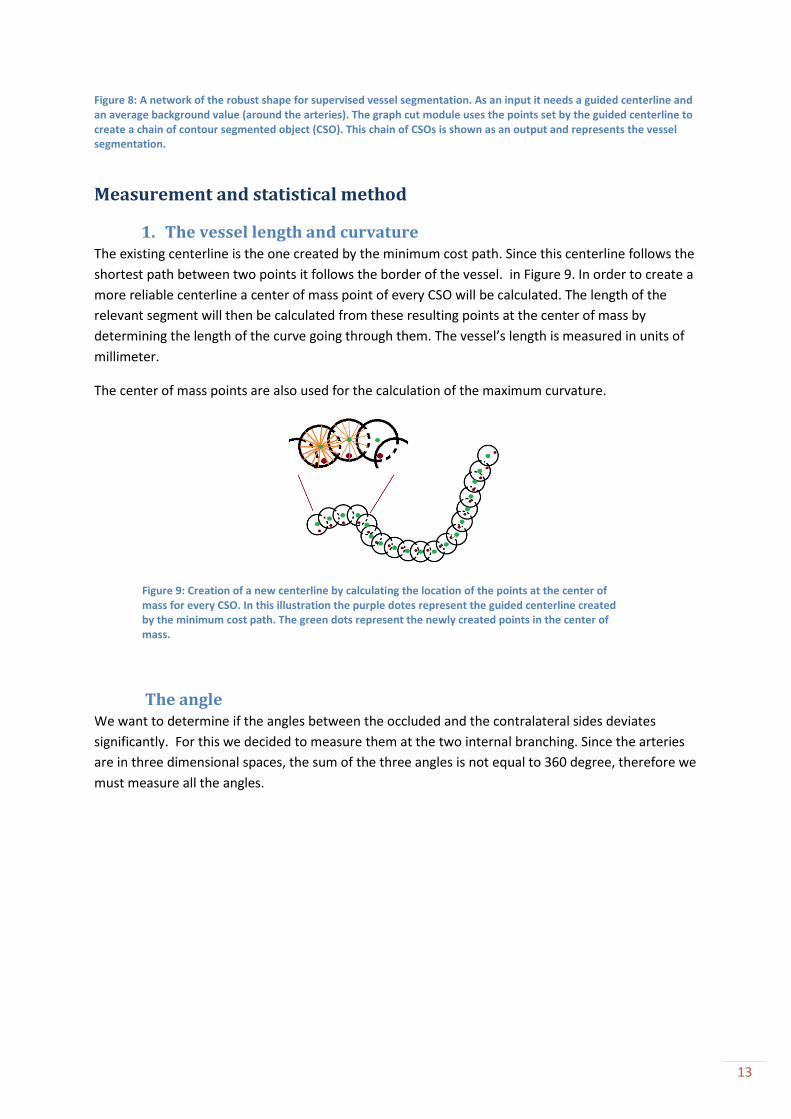
Figure 8: A network of the robust shape for supervised vessel segmentation. As an input it needs a guided centerline and an average background value (around the arteries). The graph cut module uses the points set by the guided centerline to create a chain of contour segmented object (CSO). This chain of CSOs is shown as an output and represents the vessel segmentation.
Measurement and statistical method
1. The vessel length and curvature The existing centerline is the one created by the minimum cost path. Since this centerline follows the
shortest path between two points it follows the border of the vessel. in Figure 9. In order to create a
more reliable centerline a center of mass point of every CSO will be calculated. The length of the
relevant segment will then be calculated from these resulting points at the center of mass by
determining the length of the curve going through them. The vessel’s length is measured in units of
millimeter.
The center of mass points are also used for the calculation of the maximum curvature.
Figure 9: Creation of a new centerline by calculating the location of the points at the center of mass for every CSO. In this illustration the purple dotes represent the guided centerline created by the minimum cost path. The green dots represent the newly created points in the center of mass.
The angle We want to determine if the angles between the occluded and the contralateral sides deviates
significantly. For this we decided to measure them at the two internal branching. Since the arteries
are in three dimensional spaces, the sum of the three angles is not equal to 360 degree, therefore we
must measure all the angles.

14
Figure 8: Illustration A is an example of how the angles of a real artery would be measured. Illustration B defines the angles and the segments. Where; S1 is the ICA, S2 the proximal M1, S3 and S4 The proximal M2, and S5 the A1 segment of the ACA
The radius The radius is measured by using the CSOs obtain from the robust kernel segmentation. Since a vessel
consists of many such CSOs a large dataset of radii is obtained. From this dataset the minimum,
maximum and average value are extracted. Since they are independent to the variation in the vessel
length.
Pearson correlation coefficient The Pearson correlation coefficient r gives a measure to what extent two variables1, X and Y, have a
linear correlation between each other. The correlation coefficient can take any value in the
interval [-1, +1]. The magnitude of the r value gives a measure to how strongly correlated the two
variables X and Y are.
A positive coefficient (r) tells us that when the variable X increases, the variable Y also increase. The
opposite happens when the correlation coefficient is negative, because if variable X increases the
variable Y decreases. A correlation coefficient of zero indicates that there is no correlation between
the variables X and Y.
The correlation coefficient alone is not sufficient to give any meaning to how the two variables are
related. Since the correlation can happen by chance. So to avoid collecting meaningless correlations
the measurements also contain a significance level 0 < p ≤ 0.05. If the probability value p for the
correlation is smaller than 0.05 then it is called significant.
Paired T-test A paired T-test is a hypothesis test between two dependent variables X and Y. The null hypothesis
needs to be rejected and the alternative hypothesis accepted if there is a significantly difference in
the average values between the two variables. Thus, for such an hypothesis test we calculate to what
probability value (or p-value) the average values ̅ and ̅ differ from each other. If the calculated
value is equal or smaller than 0.05, which correspond to a Confidence interval (CI) of 95%, then we
say that these variables X and Y are significantly different. 1 With variables it is meant all the angles, maximum curvatures, lengths, and radii.

15
Results
For this project we received 104 MR Clean patients. Which contained 104 baseline CTAs and 75
follow up CTAs. Of all follow up CTAs Only 25 were fully recanalized. Since we want to restrict the
amount of CTAs with artifacts and noise in it. So the Exclusion criteria is being applied.
After the exclusion criteria only 65 baseline CTAs and 18 (fully recanalized) follow up CTAs remain.
Correlation and significance
For 108 pairs of variables a significant correlation was found. Of these 108 pairs of variables 62 pairs
have a moderate to high correlation coefficient and also contain an high2 level of significance, as seen
in Table 1.
Of the 61 sets of paired variables 50 pairs correspond to inter radial correlations. The lengths of the
proximal M1 and the two proximal M2 segments are moderate correlated with their own segmental
maximum curvature (with an high level of significance).
Table 1: This table shows the correlation coefficient (r) related to a classification. It also contains how many pairs of variables are related to a certain correlation coefficient and significance level. [8]
Further obtained data for the correlations is placed in appendix B. In appendix C a matrix containing
Paired T-test
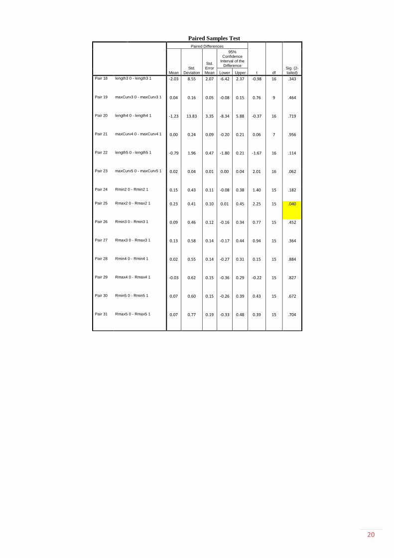
The paired T-test shows us that of the 31 pairs 7 pairs of variables are significantly different. Of the
significantly different pairs three of them correspond to the radius of the internal carotid artery.
2 High significance means a significance level of p≤0.01.
Correlation coefficient r Classification Amount of pairs
0 ≤ 0.35 low/weak 35*
0 ≤ 0.35 low/weak 12**
0.36 - 0.67 moderate 55**
0.68 - 1.00 strong/high 6**
≥ 0.90 very high 0
**significance p ≤ 0.01 *significance 0.01< p ≤ 0.05

16
Table 2: This table contains the 7 pairs which are significantly different.
Discussion
Relations between the arteries
The measurements of the correlations between the arteries have been completed with success.
Significant correlations were found in 107 pairs of variables. With an amount of 56 pairs of variables
containing a moderate correlation and 5 pairs of variables containing a strong correlation both with a
p-value of less than 1%.
Linear models can be created. But, the creation of the linear models was beyond the scope of this
project. Since, finding significant correlation between the artery’s properties and to measure
symmetry in the complete circle of Willis was the main point of research.
Symmetry in the proximal arteries
We have measured symmetry with the paired T-test and found 7 variable pairs which were
significant different. The remaining 24 variable pairs that are not significantly different can be
interpreted as to not being different to each other. However, since we didn’t measure the actual
equalness with the T-test between the 24 variables we don’t actually know to what significance level
these variables are equal.
The available set of 18 useful CTA scans is also relatively low to obtain a robust and meaningful
outcome. Nonetheless, it gives us
Limitations
The minimum cost path failed to generated a few guided centerlines. Due to a skull mask which did
not cover the skull sufficiently. In which the Vesselness filter the uncovered parts of the skull used as
if it was an vessel. Because of this some guided centerlines needed to be annotated manually.
Lower Upper
Pair 4 Angle x 0 - Angle x 1 -20.15 32.79 7.95 -37.01 -3.29 -2.53 16 .022
Pair 5 Angle α 0 - Angle α 1 -12.94 14.66 4.64 -23.43 -2.46 -2.79 9 .021
Pair 7 Rmin1 0 - Rmin1 1 -.214 .416 .101 -.428 .000 -2.12 16 .050
Pair 8 Rmax1 0 - Rmax1 1 -.429 .384 .093 -.627 -.231 -4.60 16 .000
Pair 9 Raverage1 0 - Raverage1 1 -.346 .392 .095 -.548 -.145 -3.64 16 .002
Pair 14 length1 0 - length1 1 -6.08187 10.93633 2.82375 -12.13820 -.02553 -2.154 14 .049
Pair 25 Rmax2 0 - Rmax2 1 .22914 .40767 .10192 .01191 .44638 2.248 15 .040
Paired Differences
t df
Sig. (2-
tailed)Mean
Std.
Deviation
Std. Error
Mean
95% Confidence
Interval of the
Paired Samples Test

17
Moreover, measurements of the internal carotid artery and the anterior cerebral artery failed in 18
MR Clean patients due to some internal failure of the Robust kernel segmentation.
The dimensions of the arteries in the fully recanalized follow up CTA could also be affected by the
intravenous treatment done during the surgery. Due to this it could be that the vessels are swollen
up and a little bit moved from its actual location at the time the patient gets its follow up CTA scan.
Conclusion
61 pairs of variables containing a moderate to high correlation with also a significance value p smaller
than 1%. For these pairs of variables determination of linear equation is possible.
Validation of the linear equations can be done by predicting the values on a test set of new patients.
We measured symmetry. But, from our results we can conclude that only 7 of the 31 paired
variables, as seen in the tables of Appendix A. Are significant different. The remaining 24 pairs could
be interpreted as not different, but there is no value of significance
Since the symmetry measurements relay on a small amount of data. It is advisable when further
study in symmetry is going to be done to at least use a larger data set of recanalized follow up CTAs.
Or rather to do the symmetry study with a large data set of healthy blood vessels of the Circle of
Willis.
Epilogue I chose to do this bachelor thesis about “symmetry and relations in the proximal arteries of ischemic
stroke patients” at the AMC, because I wanted to extent my view in science. Since, in the first three
years of my physics program I only got in touch with astronomy and physics courses.
During my bachelor project I learnt many new terminology from the field of biomedical engineering.
Especially in the area of imaging and visualization of the brain. Where I needed to work with the
programming software MeVisLab. Which can be used to build networks consisting of modules for
measurements and visualization purposes. After struggling a lot in the previous month I eventually
managed to build my own networks.
I want to specially thank my supervisor Emillie M. Santos who helped me a lot during my project with
both the project itself as with my presentation.

18
References
[1] Emilie M.M., et al., “Symmetry based computer aided segmentation of occluded cerebral arteries
on CT Angiography”, IFBME proceedings, 2014, volume 41, 4 pages.
[2] Michiel Schaap, et al., “Robust Shape Regression for Supervised Vessel Segmentation and its
applications to coronary Segmentation in CTA”, IEEE Transactions on medical imaging, 2011, issue
11/ volume: 30, 13 pages.
[3] C.T. Metz, et al., ”Two Point Minimum Cost Approach for CTA Coronary Centerline Extraction”,
MIDAS Journal, 2008, 7 pages.
[4] Lawton, Michael T. MD, Seven Aneurysms: Tenets and Techniques for Clipping, Kay Conerly,
Thieme Medical Publishers, New York, 2011.
[5] By Leslie Ritter, PhD, RN, and Bruce Coull, MD, University of Arizona;
http://heart.arizona.edu/heart-health/preventing-stroke/lowering-risks-stroke
[6] A. W. J. Hoksbergen, “Collateral Variations in Circle of Willis in Atherosclerotic Population
Assessed by Means of Transcranial Color-Coded Duplex Ultrasonography”, Chris Bor, Febodruk BV
Enschede, Enschede, 2003.
[7] Christian H. Riedel, et al., “The Importance of Size: Succesful Recanalization by intravenous
Thrombolysis in acute Anterior Stroke Depends on thrombus Length”, Stroke, 2011, volume 42, 4.
[8] Richard Taylor, EDD, RDCS, “Interpretation of the Correlation Coefficient: A Basic Review”, JDSM,
1990, volume 1, 5 pages.

19
Appendix A This appendix contain all relevant data of the symmetry measurements.
Lower Upper
Pair 1 1.7 12.82 3.11 -4.89 8.29 0.55 16 0.592
Pair 2 -1.6 8.7 2.62 -7.45 4.25 -0.61 10 0.556
Pair 3 -17.09 34.56 8.38 -34.85 0.68 -2.04 16 0.058
Pair 4 -20.15 32.79 7.95 -37.01 -3.29 -2.53 16 0.022
Pair 5 -12.94 14.66 4.64 -23.43 -2.46 -2.79 9 0.021
Pair 6 -6.85 39.95 9.69 -27.39 13.69 -0.71 16 0.49
Pair 7 -0.21 0.42 0.1 -0.43 0 -2.12 16 0.05
Pair 8 -0.43 0.38 0.09 -0.63 -0.23 -4.6 16 0
Pair 9 -0.35 0.39 0.1 -0.55 -0.14 -3.64 16 0.002
Pair 10 0.17 0.42 0.1 -0.04 0.38 1.67 16 0.114
Pair 11 0.1 0.49 0.12 -0.15 0.35 0.86 16 0.4
Pair 12 -0.01 0.55 0.13 -0.29 0.28 -0.04 16 0.967
Pair 13 0.05 0.66 0.16 -0.29 0.39 0.32 16 0.756
Pair 14 -6.08 10.94 2.82 -12.14 -0.03 -2.15 14 0.049
Pair 15 0.03 0.12 0.03 -0.04 0.1 0.98 14 0.343
Pair 16 3.58 8.11 2.03 -0.74 7.91 1.77 15 0.098
Pair 17 0.09 0.16 0.06 -0.04 0.23 1.61 7 0.151
length2 0 - length2 1
maxCurv2 0 - maxCurv2 1
Paired Samples Test
Raverage3 0 - Raverage3 1
Raverage4 0 - Raverage4 1
Raverage5 - Raverage5 1
length1 0 - length1 1
maxCurv1 0 - maxCurv1 1
Angle g 0 - Angle g 1
Angle b 0 – Angle b 1
Angle d 0 – Angle d 1
Angle x 0 – Angle x 1
Angle a 0 – Angle a 1
Angle z 0 – Angle z 1
Rmin1 0 - Rmin1 1
Rmax1 0 - Rmax1 1
Raverage1 0 - Raverage1 1
Raverage2 0 - Raverage2 1
Paired Differences
t df Sig. (2- tailed)
Mean Std. Deviation Std. Error Mean
95% Confidence Interval of the
Difference
20
Paired Samples Test
Paired Differences
t df Sig. (2-tailed) Mean
Std. Deviation
Std. Error Mean
95% Confidence
Interval of the Difference
Lower Upper
Pair 18 length3 0 - length3 1 -2.03 8.55 2.07 -6.42 2.37 -0.98 16 .343
Pair 19 maxCurv3 0 - maxCurv3 1 0.04 0.16 0.05 -0.08 0.15 0.76 9 .464
Pair 20 length4 0 - length4 1 -1.23 13.83 3.35 -8.34 5.88 -0.37 16 .719
Pair 21 maxCurv4 0 - maxCurv4 1 0.00 0.24 0.09 -0.20 0.21 0.06 7 .956
Pair 22 length5 0 - length5 1 -0.79 1.96 0.47 -1.80 0.21 -1.67 16 .114
Pair 23 maxCurv5 0 - maxCurv5 1 0.02 0.04 0.01 0.00 0.04 2.01 16 .062
Pair 24 Rmin2 0 - Rmin2 1 0.15 0.43 0.11 -0.08 0.38 1.40 15 .182
Pair 25 Rmax2 0 - Rmax2 1 0.23 0.41 0.10 0.01 0.45 2.25 15 .040
Pair 26 Rmin3 0 - Rmin3 1 0.09 0.46 0.12 -0.16 0.34 0.77 15 .452
Pair 27 Rmax3 0 - Rmax3 1 0.13 0.58 0.14 -0.17 0.44 0.94 15 .364
Pair 28 Rmin4 0 - Rmin4 1 0.02 0.55 0.14 -0.27 0.31 0.15 15 .884
Pair 29 Rmax4 0 - Rmax4 1 -0.03 0.62 0.15 -0.36 0.29 -0.22 15 .827
Pair 30 Rmin5 0 - Rmin5 1 0.07 0.60 0.15 -0.26 0.39 0.43 15 .672
Pair 31 Rmax5 0 - Rmax5 1 0.07 0.77 0.19 -0.33 0.48 0.39 15 .704
21
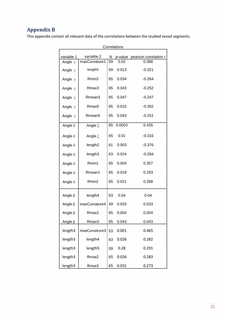
Appendix B This appendix contain all relevant data of the correlations between the studied vessel segments.
Correlations
variable 1 variable 2 N p-value pearson correlation r
Angle g maxCurvature1 59 0.02 0.388
Angle g length5 59 0.013 -0.321
Angle g Rmin3 65 0.034 -0.264
Angle g Rmax3 65 0.043 -0.252
Angle g Rmean3 65 0.047 -0.247
Angle g Rmax5 65 0.015 -0.302
Angle g Rmean5 65 0.043 -0.251
Angle d Angle x 65 0.0003 0.435
Angle d Angle z 65 0.01 -0.316
Angle d length2 61 0.003 -0.376
Angle d length3 63 0.024 -0.284
Angle d Rmin1 65 0.004 0.357
Angle d Rmean1 65 0.018 0.293
Angle d Rmin2 65 0.021 0.288
Angle b length4 63 0.04 0.04
Angle b maxCurvature4 49 0.033 0.033
Angle b Rmax1 65 0.004 0.004
Angle b Rmax3 65 0.043 0.043
length3 maxCurvature3 53 0.001 0.465
length3 length4 63 0.026 0.282
length3 length5 59 0.28 0.291
length3 Rmax2 65 0.026 0.283
length3 Rmax3 65 0.031 0.273

22
Correlations
variable 1 variable 2 N p-value pearson
correlation r
Angle x Angle z 65 0.000 -0.552
Angle x Rmin1 65 0.009 0.322
Angle x Rmean1 65 0.004 0.35
Angle z length4 63 0.002 -0.374
Angle z maxCurvature4 49 0.050 -0.282
Angle z Rmin1 65 0.016 -0.298
Angle z Rmax1 65 0.019 -0.29
Angle z Rmean1 65 0.004 -0.357
Angle z Rmin2 65 0.015 -0.303
Angle z Rmean2 65 0.031 -0.269
maxCurvature1 length3 63 0.010 -0.334
length2 maxCurvature2 57 0.000 0.543
length2 Rmax2 65 0.030 0.377
maxCurvature2 length3 63 0.043 0.272
maxCurvature2 Rmin1 65 0.037 -0.277
maxCurvature2 Rmax2 65 0.000 0.454
maxCurvature2 Rmean2 65 0.009 0.344
maxCurvature2 Rmax3 65 0.017 0.314
maxCurvature2 Rmean3 65 0.041 0.271
maxCurvature3 Rmax3 65 0.013 0.346
maxCurvature3 Rmean3 65 0.042 0.286

23
Correlations
variable 1 variable 2 N p-value pearson
correlation r
length4 maxCurvature4 49 0.009 0.369
length4 Rmax1 65 0.031 0.271
length4 Rmean1 65 0.010 0.323
length4 Rmax2 65 0.016 0.305
length4 Rmean2 65 0.031 0.272
Rmin1 Rmax1 65 0.000 0.493
Rmin1 Rmean1 65 0.000 0.765
Rmax1 Rmean1 65 0.000 0.86
Rmax1 Rmax3 65 0.006 -0.335
Rmax1 Rmean3 65 0.014 -0.303
Rmean1 Rmax3 65 0.012 -0.309
Rmean1 Rmean3 65 0.026 -0.276
Rmin2 Rmax2 65 0.000 0.666
Rmin2 Rmean2 65 0.000 0.912
Rmin2 Rmin3 65 0.000 0.428
Rmin2 Rmax3 65 0.000 0.464
Rmin2 Rmean3 65 0.000 0.48
Rmin2 Rmin4 65 0.000 0.514
Rmin2 Rmax4 65 0.000 0.532
Rmin2 Rmean4 65 0.000 0.529
Rmin2 Rmin5 65 0.000 0.407
Rmin2 Rmax5 65 0.000 0.489
Rmin2 Rmean5 65 0.000 0.456
Rmax2 Rmean2 65 0.000 0.907
Rmax2 Rmin3 65 0.026 0.277
Rmax2 Rmax3 65 0.003 0.368
Rmax2 Rmean3 65 0.004 0.357
Rmax2 Rmin4 65 0.004 0.355
Rmax2 Rmax4 65 0.001 0.417
Rmax2 Rmean4 65 0.002 0.385
Rmax2 Rmin5 65 0.005 0.345
Rmax2 Rmax5 65 0.001 0.398
Rmax2 Rmean5 65 0.002 0.373

24
Appendix C The matrix below contains all correlations between the variables. The meaningful correlations are
colored.
Angle g Angle b Angle d Angle x Angle a Angle z length1
maxCurvat
ure1 length2
maxCurvat
ure2 length3
maxCurvat
ure3 length4
maxCurvat
ure4 length5
maxCurvat
ure5 Rmin1 Rmax1 Rmean1 Rmin2 Rmax2 Rmean2 Rmin3 Rmax3 Rmean3 Rmin4 Rmax4 Rmean4 Rmin5 Rmax5 Rmean5
Pearson
Correlation
1 .017 .146 -.047 .045 .073 -.208 .388** -.030 -.143 -.075 .123 .088 -.224 -.321* -.058 .115 .099 .085 -.125 .007 -.078 -.264* -.252* -.247* -.107 -.147 -.121 -.205 -.302* -.251*
Sig. (2-
tailed)
.891 .247 .712 .720 .565 .108 .002 .817 .287 .560 .388 .493 .121 .013 .665 .362 .432 .502 .324 .958 .539 .034 .043 .047 .396 .244 .338 .102 .015 .043
Pearson
Correlation
.017 1 .037 .011 .150 .027 -.159 -.063 -.022 -.024 -.144 -.085 -.260* -.305* -.192 -.095 .066 .352** .213 -.231 -.213 -.242 -.145 -.252* -.241 -.002 -.051 -.035 -.029 -.115 -.062
Sig. (2-
tailed)
.891 .768 .929 .234 .831 .222 .635 .864 .858 .259 .555 .040 .033 .146 .474 .602 .004 .089 .066 .091 .052 .248 .043 .053 .985 .685 .782 .817 .361 .624
Pearson
Correlation
.146 .037 1 .435** -.068 -.316* .018 .021 -.376** -.254 -.284* -.084 .167 -.150 -.221 -.088 .357** .160 .293* .288* .036 .163 .162 -.062 .041 .106 .102 .093 .026 .036 .047
Sig. (2-
tailed)
.247 .768 .000 .588 .010 .891 .873 .003 .056 .024 .558 .192 .303 .093 .507 .004 .202 .018 .021 .776 .193 .198 .626 .743 .398 .421 .460 .837 .775 .713
Pearson
Correlation
-.047 .011 .435** 1 -.162 -.552** .077 .108 -.200 -.145 -.059 .080 .205 -.006 .009 -.013 .322** .192 .350** .138 -.039 .066 .165 .061 .112 .049 .080 .064 -.027 .010 -.005
Sig. (2-
tailed)
.712 .929 .000 .198 .000 .553 .417 .123 .281 .644 .577 .108 .966 .949 .923 .009 .125 .004 .276 .762 .599 .189 .629 .373 .701 .525 .614 .830 .936 .970
Pearson
Correlation
.045 .150 -.068 -.162 1 .056 -.154 -.111 .107 -.172 -.061 -.129 -.166 -.020 -.131 -.221 -.080 .008 -.020 -.220 -.104 -.181 -.196 -.104 -.139 -.153 -.082 -.112 .005 -.046 -.023
Sig. (2-
tailed)
.720 .234 .588 .198 .656 .236 .404 .412 .201 .634 .368 .194 .893 .324 .092 .528 .949 .874 .081 .413 .150 .117 .410 .271 .225 .517 .373 .970 .719 .859
Pearson
Correlation
.073 .027 -.316* -.552** .056 1 -.065 .058 .170 -.083 -.185 -.126 -.374** -.282* -.113 .081 -.298* -.290* -.357** -.303* -.189 -.269* -.168 -.179 -.194 -.148 -.226 -.191 -.121 -.149 -.138
Sig. (2-
tailed)
.565 .831 .010 .000 .656 .617 .661 .189 .538 .147 .378 .002 .050 .394 .543 .016 .019 .004 .015 .134 .031 .180 .153 .121 .238 .070 .128 .339 .235 .274
Pearson
Correlation
-.208 -.159 .018 .077 -.154 -.065 1 -.029 -.002 -.057 .177 .064 .181 .244 .098 -.070 .176 .033 .181 -.134 -.111 -.135 -.007 .060 .004 .000 .038 .016 .036 .044 .042
Sig. (2-
tailed)
.108 .222 .891 .553 .236 .617 .827 .991 .686 .175 .667 .171 .102 .478 .610 .176 .799 .163 .306 .399 .298 .954 .645 .978 .999 .771 .901 .782 .734 .749
Pearson
Correlation.388** -.063 .021 .108 -.111 .058 -.029 1 -.005 -.212 -.334* -.273 .014 -.089 -.013 .173 -.015 -.075 -.048 -.100 -.075 -.081 -.201 -.184 -.201 -.098 -.136 -.115 -.074 -.046 -.073
Sig. (2-
tailed)
.002 .635 .873 .417 .404 .661 .827 .971 .135 .010 .064 .918 .566 .924 .215 .908 .574 .720 .455 .576 .542 .127 .163 .126 .459 .303 .384 .579 .731 .585
Pearson
Correlation
-.030 -.022 -.376** -.200 .107 .170 -.002 -.005 1 .543** .211 -.101 -.111 -.028 -.178 .044 -.114 .019 -.089 -.237 .377** .100 -.094 -.026 -.054 -.098 -.078 -.088 .078 .036 .052
Sig. (2-
tailed)
.817 .864 .003 .123 .412 .189 .991 .971 .000 .106 .489 .397 .851 .193 .749 .380 .885 .494 .068 .003 .441 .472 .843 .679 .453 .551 .499 .549 .784 .690
Pearson
Correlation
-.143 -.024 -.254 -.145 -.172 -.083 -.057 -.212 .543** 1 .272* .073 .172 .076 .000 .045 -.277* .092 -.134 .133 .454** .344** .194 .314* .271* .155 .213 .179 .241 .217 .236
Sig. (2-
tailed)
.287 .858 .056 .281 .201 .538 .686 .135 .000 .043 .635 .205 .633 .998 .756 .037 .495 .322 .329 .000 .009 .147 .017 .041 .249 .111 .183 .071 .105 .077
Pearson
Correlation
-.075 -.144 -.284* -.059 -.061 -.185 .177 -.334* .211 .272* 1 .465** .282* .205 .291* .045 .102 .092 .051 .109 .283* .214 .104 .273* .226 .135 .206 .182 .174 .163 .188
Sig. (2-
tailed)
.560 .259 .024 .644 .634 .147 .175 .010 .106 .043 .001 .026 .163 .028 .741 .425 .473 .692 .399 .026 .092 .419 .031 .074 .291 .105 .155 .173 .202 .140
Pearson
Correlation
.123 -.085 -.084 .080 -.129 -.126 .064 -.273 -.101 .073 .465** 1 .043 -.077 -.021 -.129 .330
* .088 .149 .186 .090 .151 .173 .346*
.286* .131 .140 .148 .105 .024 .088
Sig. (2-
tailed)
.388 .555 .558 .577 .368 .378 .667 .064 .489 .635 .001 .765 .646 .891 .398 .018 .538 .298 .196 .533 .289 .224 .013 .042 .361 .328 .299 .464 .868 .537
Pearson
Correlation
.088 -.260* .167 .205 -.166 -.374** .181 .014 -.111 .172 .282* .043 1 .369** -.005 .009 .151 .271* .323** .211 .305* .272* -.057 .028 .004 -.072 .097 .008 .000 -.009 -.006
Sig. (2-
tailed)
.493 .040 .192 .108 .194 .002 .171 .918 .397 .205 .026 .765 .009 .968 .949 .237 .031 .010 .100 .016 .031 .656 .830 .974 .573 .447 .950 .999 .945 .965
Pearson
Correlation
-.224 -.305* -.150 -.006 -.020 -.282* .244 -.089 -.028 .076 .205 -.077 .369** 1 .140 .254 -.003 -.139 -.002 .071 .062 .078 .067 .212 .177 -.224 -.095 -.143 -.035 .095 .018
Sig. (2-
tailed)
.121 .033 .303 .966 .893 .050 .102 .566 .851 .633 .163 .646 .009 .372 .100 .986 .341 .987 .632 .675 .595 .646 .144 .223 .121 .516 .326 .810 .516 .903
Pearson
Correlation-.321* -.192 -.221 .009 -.131 -.113 .098 -.013 -.178 .000 .291* -.021 -.005 .140 1 .132 -.129 .015 -.079 .193 .052 .132 -.089 -.002 -.066 .068 .034 .047 -.043 .137 .045
Sig. (2-
tailed)
.013 .146 .093 .949 .324 .394 .478 .924 .193 .998 .028 .891 .968 .372 .319 .330 .907 .553 .148 .697 .318 .504 .988 .617 .606 .796 .726 .748 .299 .734
Pearson
Correlation
-.058 -.095 -.088 -.013 -.221 .081 -.070 .173 .044 .045 .045 -.129 .009 .254 .132 1 -.054 -.196 -.185 -.007 -.065 -.031 -.091 .089 .000 -.052 -.047 -.050 .082 .177 .127
Sig. (2-
tailed)
.665 .474 .507 .923 .092 .543 .610 .215 .749 .756 .741 .398 .949 .100 .319 .684 .136 .160 .959 .627 .817 .495 .503 .998 .698 .725 .709 .539 .180 .339
Pearson
Correlation
.115 .066 .357** .322** -.080 -.298* .176 -.015 -.114 -.277* .102 .330* .151 -.003 -.129 -.054 1 .493** .765** .009 -.132 -.062 -.139 -.135 -.122 -.167 -.122 -.135 -.114 -.154 -.127
Sig. (2-
tailed)
.362 .602 .004 .009 .528 .016 .176 .908 .380 .037 .425 .018 .237 .986 .330 .684 .000 .000 .945 .297 .623 .271 .282 .334 .182 .332 .284 .367 .221 .312
Pearson
Correlation
.099 .352** .160 .192 .008 -.290* .033 -.075 .019 .092 .092 .088 .271* -.139 .015 -.196 .493** 1 .860** -.038 .028 -.005 -.243 -.335** -.303* -.153 -.107 -.135 -.155 -.225 -.176
Sig. (2-
tailed)
.432 .004 .202 .125 .949 .019 .799 .574 .885 .495 .473 .538 .031 .341 .907 .136 .000 .000 .764 .825 .970 .051 .006 .014 .223 .395 .285 .218 .071 .161
Pearson
Correlation
.085 .213 .293* .350** -.020 -.357** .181 -.048 -.089 -.134 .051 .149 .323** -.002 -.079 -.185 .765** .860** 1 -.065 -.097 -.084 -.228 -.309* -.276* -.235 -.166 -.201 -.162 -.234 -.190
Sig. (2-
tailed)
.502 .089 .018 .004 .874 .004 .163 .720 .494 .322 .692 .298 .010 .987 .553 .160 .000 .000 .608 .447 .508 .068 .012 .026 .059 .185 .109 .196 .061 .129
Pearson
Correlation
-.125 -.231 .288* .138 -.220 -.303* -.134 -.100 -.237 .133 .109 .186 .211 .071 .193 -.007 .009 -.038 -.065 1 .666** .912** .428** .464** .480** .514** .532** .529** .407** .489** .456**
Sig. (2-
tailed)
.324 .066 .021 .276 .081 .015 .306 .455 .068 .329 .399 .196 .100 .632 .148 .959 .945 .764 .608 .000 .000 .000 .000 .000 .000 .000 .000 .001 .000 .000
Pearson
Correlation
.007 -.213 .036 -.039 -.104 -.189 -.111 -.075 .377** .454** .283* .090 .305* .062 .052 -.065 -.132 .028 -.097 .666** 1 .907** .277* .368** .357** .355** .417** .385** .345** .398** .373**
Sig. (2-
tailed)
.958 .091 .776 .762 .413 .134 .399 .576 .003 .000 .026 .533 .016 .675 .697 .627 .297 .825 .447 .000 .000 .026 .003 .004 .004 .001 .002 .005 .001 .002
Pearson
Correlation
-.078 -.242 .163 .066 -.181 -.269* -.135 -.081 .100 .344** .214 .151 .272* .078 .132 -.031 -.062 -.005 -.084 .912** .907** 1 .379** .454** .454** .473** .519** .499** .415** .484** .455**
Sig. (2-
tailed)
.539 .052 .193 .599 .150 .031 .298 .542 .441 .009 .092 .289 .031 .595 .318 .817 .623 .970 .508 .000 .000 .002 .000 .000 .000 .000 .000 .001 .000 .000
Pearson
Correlation-.264* -.145 .162 .165 -.196 -.168 -.007 -.201 -.094 .194 .104 .173 -.057 .067 -.089 -.091 -.139 -.243 -.228 .428** .277* .379** 1 .806** .933** .540** .508** .522** .486** .461** .499**
Sig. (2-
tailed)
.034 .248 .198 .189 .117 .180 .954 .127 .472 .147 .419 .224 .656 .646 .504 .495 .271 .051 .068 .000 .026 .002 .000 .000 .000 .000 .000 .000 .000 .000
Pearson
Correlation-.252* -.252* -.062 .061 -.104 -.179 .060 -.184 -.026 .314* .273* .346* .028 .212 -.002 .089 -.135 -.335** -.309* .464** .368** .454** .806** 1 .954** .570** .608** .601** .530** .543** .558**
Sig. (2-
tailed)
.043 .043 .626 .629 .410 .153 .645 .163 .843 .017 .031 .013 .830 .144 .988 .503 .282 .006 .012 .000 .003 .000 .000 .000 .000 .000 .000 .000 .000 .000
Pearson
Correlation-.247* -.241 .041 .112 -.139 -.194 .004 -.201 -.054 .271* .226 .286* .004 .177 -.066 .000 -.122 -.303* -.276* .480** .357** .454** .933** .954** 1 .573** .592** .592** .521** .520** .545**
Sig. (2-
tailed)
.047 .053 .743 .373 .271 .121 .978 .126 .679 .041 .074 .042 .974 .223 .617 .998 .334 .014 .026 .000 .004 .000 .000 .000 .000 .000 .000 .000 .000 .000
Pearson
Correlation
-.107 -.002 .106 .049 -.153 -.148 .000 -.098 -.098 .155 .135 .131 -.072 -.224 .068 -.052 -.167 -.153 -.235 .514** .355** .473** .540** .570** .573** 1 .958** .986** .682** .688** .714**
Sig. (2-
tailed)
.396 .985 .398 .701 .225 .238 .999 .459 .453 .249 .291 .361 .573 .121 .606 .698 .182 .223 .059 .000 .004 .000 .000 .000 .000 .000 .000 .000 .000 .000
Pearson
Correlation
-.147 -.051 .102 .080 -.082 -.226 .038 -.136 -.078 .213 .206 .140 .097 -.095 .034 -.047 -.122 -.107 -.166 .532** .417** .519** .508** .608** .592** .958** 1 .990** .665** .676** .697**
Sig. (2-
tailed)
.244 .685 .421 .525 .517 .070 .771 .303 .551 .111 .105 .328 .447 .516 .796 .725 .332 .395 .185 .000 .001 .000 .000 .000 .000 .000 .000 .000 .000 .000
Pearson
Correlation
-.121 -.035 .093 .064 -.112 -.191 .016 -.115 -.088 .179 .182 .148 .008 -.143 .047 -.050 -.135 -.135 -.201 .529** .385** .499** .522** .601** .592** .986** .990** 1 .676** .680** .706**
Sig. (2-
tailed)
.338 .782 .460 .614 .373 .128 .901 .384 .499 .183 .155 .299 .950 .326 .726 .709 .284 .285 .109 .000 .002 .000 .000 .000 .000 .000 .000 .000 .000 .000
Pearson
Correlation
-.205 -.029 .026 -.027 .005 -.121 .036 -.074 .078 .241 .174 .105 .000 -.035 -.043 .082 -.114 -.155 -.162 .407** .345** .415** .486** .530** .521** .682** .665** .676** 1 .892** .976**
Sig. (2-
tailed)
.102 .817 .837 .830 .970 .339 .782 .579 .549 .071 .173 .464 .999 .810 .748 .539 .367 .218 .196 .001 .005 .001 .000 .000 .000 .000 .000 .000 .000 .000
Pearson
Correlation-.302* -.115 .036 .010 -.046 -.149 .044 -.046 .036 .217 .163 .024 -.009 .095 .137 .177 -.154 -.225 -.234 .489** .398** .484** .461** .543** .520** .688** .676** .680** .892** 1 .964**
Sig. (2-
tailed)
.015 .361 .775 .936 .719 .235 .734 .731 .784 .105 .202 .868 .945 .516 .299 .180 .221 .071 .061 .000 .001 .000 .000 .000 .000 .000 .000 .000 .000 .000
Pearson
Correlation-.251* -.062 .047 -.005 -.023 -.138 .042 -.073 .052 .236 .188 .088 -.006 .018 .045 .127 -.127 -.176 -.190 .456** .373** .455** .499** .558** .545** .714** .697** .706** .976** .964** 1
Sig. (2-
tailed)
.043 .624 .713 .970 .859 .274 .749 .585 .690 .077 .140 .537 .965 .903 .734 .339 .312 .161 .129 .000 .002 .000 .000 .000 .000 .000 .000 .000 .000 .000
N 65 65 65 65 65 65 61 59 61 57 63 51 63 49 59 59 65 65 65 64 64 65 65 65 65 65 65 65 65 65 65
Pearson Correlation Pearson Correlation Pearson Correlation Pearson Correlation
0 ≤ 0.35* 0** ≤ 0.35** 0.36** - 0.67** 0.68** - 1.00**
length2
Correlations
Angle g
Angle b
Angle d
Angle x
Angle a
Angle z
length1
maxCurvat
ure1
Rmax2
maxCurvat
ure2
length3
maxCurvat
ure3
length4
maxCurvat
ure4
length5
maxCurvat
ure5
Rmin1
Rmax1
Rmean1
Rmin2
*. Correlation is significant at the 0.05 level (2-tailed).
Rmean2
Rmin3
Rmax3
Rmean3
Rmin4
Rmax4
Rmean4
Rmin5
Rmax5
Rmean5
**. Correlation is significant at the 0.01 level (2-tailed).

25
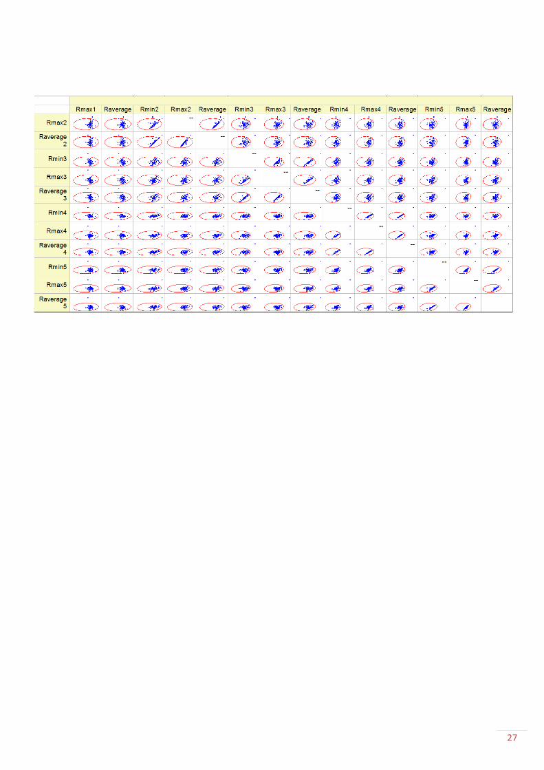
Appendix D The matrices below show all possible scatterplots. The scatterplots are drawn together with a
Confidens Ellips. (The confidence level for the Ellipse is 95%.) .The four Scatter Matrices correspond
to the Pearson correlation values in the table of Appendix C.

26
27