Symmetry and Symplectic Reduction

Matthew O’Callaghan

May 2021Submitted as Part III Essay, Mathematics, Cambridge

Contents

1 Introduction 11.1 Motivation for Poisson Geometry . . . . . . . . . . . . . . . . . . . . . . . . . . . . . . . . . . 11.2 Motivation for Bianchi Lie Groups . . . . . . . . . . . . . . . . . . . . . . . . . . . . . . . . . 2

2 Lie Groups and Lie Algebras 32.1 Lie Groups . . . . . . . . . . . . . . . . . . . . . . . . . . . . . . . . . . . . . . . . . . . . . . 32.2 Representations and Actions . . . . . . . . . . . . . . . . . . . . . . . . . . . . . . . . . . . . 52.3 Classification of Three-Dimensional Lie Algebras over the Reals . . . . . . . . . . . . . . . . . 7

3 Poisson Geometry and Dynamics 103.1 Symplectic Manifolds . . . . . . . . . . . . . . . . . . . . . . . . . . . . . . . . . . . . . . . . . 103.2 Poisson Manifolds . . . . . . . . . . . . . . . . . . . . . . . . . . . . . . . . . . . . . . . . . . 113.3 Poisson Dynamics . . . . . . . . . . . . . . . . . . . . . . . . . . . . . . . . . . . . . . . . . . 133.4 Equations of Motion for g∗ . . . . . . . . . . . . . . . . . . . . . . . . . . . . . . . . . . . . . 153.5 Symplectic Foliation . . . . . . . . . . . . . . . . . . . . . . . . . . . . . . . . . . . . . . . . . 16

4 Momentum Maps and Noether’s Theorem 184.1 Momentum Maps . . . . . . . . . . . . . . . . . . . . . . . . . . . . . . . . . . . . . . . . . . . 184.2 Noether’s Theorem . . . . . . . . . . . . . . . . . . . . . . . . . . . . . . . . . . . . . . . . . . 194.3 Noether’s Theorem on g∗ . . . . . . . . . . . . . . . . . . . . . . . . . . . . . . . . . . . . . . 20

5 Reduction 225.1 Lie-Poisson Reduction . . . . . . . . . . . . . . . . . . . . . . . . . . . . . . . . . . . . . . . . 22

6 Conclusion 246.1 Concluding Remarks . . . . . . . . . . . . . . . . . . . . . . . . . . . . . . . . . . . . . . . . . 246.2 Glimpsping Further Developments: Geometric Quantization and the Orbit Method . . . . . . 24

1

Abstract

In the last hundred years, Classical Mechanics has been dwarfed by the development of Relativity andQuantum Mechanics. However, significant mathematical developments have been made to Classical Mechan-ics in the same time frame and this essay aims to explore some of the recent advances. The purpose of thisessay is to understand Hamiltonian dynamics, Noether’s theorem and symmetry in a geometric frameworkusing Poisson geometry. In particular, we want to analyse the case when the natural configuration space ofa system is a Lie group G and transformations on the space correspond to the Lie group acting on itself.In this case, the Lie-Poisson reduction theorem will say that the reduced phase space T ∗G/G is a Poissonmanifold diffeomorphic to g∗. We will begin Chapter 1 by outlining the core concepts required to understandsymmetry, in particular, we will discuss the notion of a Lie group, its Lie algebra and how each of theseobjects acts on certain manifolds. In Chapter 2 we will define Poisson and Symplectic manifolds and usethem to derive equations of motion and dynamics. Chapter 3 will discuss the geometric understanding ofNoether’s theorem by looking at momentum maps. Finally, Chapter 4 will discuss the Lie-Poisson reductiontheorem. Throughout the essay, we will aim to illustrate the concepts using the physically relevant caseswhich arise when the configuration space G is a three-dimensional Lie group over the reals.

Acknowledgements

When starting this journey in Theoretical Physics and Mathematics I never thought I would find myself inCambridge having fascinating and friendly conversations over Zoom with Dr. Jeremy Butterfield. Jeremy’sinterest in both my writing and me as a person has taught me to be more proud of my own work and totake more interest in others’; he gave me the confidence to think I had something worthwhile to write about.Thank you, Jeremy, I thoroughly enjoyed writing this essay and I enjoyed every moment in discussing thissubject with you.To all my lecturers at Trinity College, Dublin, without your teaching, I would never have attained the skillsnecessary to carry out this essay and the environment you provided for learning was second to none. Inparticular, to John Stalker, who introduced me to coadjoint orbits and representation theory; thank you foryour mentoring.To Sean Dunne, you showed me that with hard work and dedication that anything is possible; you aremissed.Finally, to my family, thank you for your continued support and for always believing in me in any decisionthat I make.

Chapter 1

Introduction

1.1 Motivation for Poisson Geometry

In courses on Classical Mechanics such as V.I. Arnold’s excellent book [6], we learn that the evolution of amechanical system with n degrees of freedom can be described in phase space coordinates

(q1(t), ..., qn(t), p1(t), ..., pn(t)), (1.1)

where qi(t), pi(t) are called the configuration and momentum coordinates respectively, via Hamilton’s equa-tions

qi(t) =∂H

∂pi, pi(t) =

∂H

∂qi, (1.2)

for a Hamiltonian H of the mechanical system. From here, one can generalise the notion of phase space andHamilton’s equations in terms of symplectic manifolds; however in this essay we will generalise Hamiltoniansystems in terms of the more general Poisson manifolds.

To motivate this we recall that we can introduce the idea of a Poisson bracket for the phase spacegeometry, namely

f, g :=

n∑i=1

(∂f

∂pi

∂g

∂qi− ∂f

∂qi∂g

∂pi); (1.3)

using this we can reformulate Hamilton’s equations as

xi(t) = H,xi(t), (1.4)

for xi one of the phase space coordinates and H a Hamiltonian. Moreover we can introduce the idea of aHamiltonian vector field by defining

XH :=

n∑i=1

(∂H

∂pi

∂

∂qi− ∂H

∂qi∂

∂pi); (1.5)

and so Equation (1.4) can be written in the form

xi(t) = XH [xi(t)]. (1.6)

We call the above development a canonical Hamiltonian system.

Our usual first step in creating an abstract framework for Hamiltonian dynamics begins by globallydescribing the dynamics in terms of a closed, nondegenerate two-form; which is embodied in the theory ofSymplectic geometry, where locally the dynamics will look like a canonical Hamiltonian system. Howeveroften we are concerned with non-canonical Hamiltonian system, which can’t be described by Symplecticgeometry; and thus Poisson manifolds were introduced to further generalize Hamiltonian dynamics to thesesystems.

1

1.2 Motivation for Bianchi Lie Groups

In Chapter 2 we will classify the three-dimensional real Lie algebras and in Chapter 3 we define a Poissonstructure on the dual to these Lie algebras g∗. The problem of classifying three-dimensional real Lie algebrasis equivalent to classifying homogeneous and anisotropic 1+3 dimensional cosmologies on spatial slices sincethe isotropy group is generated by these Lie algebras.

One can show these problems are equivalent by considering a time-slice of spacetime and letting gab bethe three-space metric on the time slice. Each time-slice being homogeneous means there exist three Killingvector fields ξi, i = 1, 2, 3, which are linearly independent at each point. The Killing vector property meansthat the three-metric is transported under the Lie derivative as

Lξi(gab) = ξci ∂cgab + gcb∂aξci + gac∂bξ

ci = 0; (1.7)

in other words, the three-metric is unchanged under transformations along integral curves of the Killingvector fields.

The Killing fields describe how the metric changes from one point in space to another and so we want toconsider the relationship between these vector fields. We do this by considering an infinitesimal closed loopby pushing along integral curves of two different vector fields and then returning in the opposite way; this isembodied in the commutator bracket of our Killing vector fields

[ξi, ξj ] = fkijξk, (1.8)

giving a Lie algebra structure to the Killing fields. Further details can be found in [7].

We will define the unique connected and simply connected Lie group associated with a three-dimensionalLie algebra as being a Bianchi group, from here we will analyse the dynamics on the dual to its Lie algebrag∗, a space which is diffeomorphic to the reduced phase space T ∗G/G as Poisson manifolds.

For the Bianchi Lie groups, the configuration space g∗ will be three dimensional therefore Symplectic ge-ometry couldn’t be used to globally describe the dynamics, since Symplectic manifolds are even-dimensional.Hence we use the theory of Poisson geometry to define Hamiltonian dynamics on this system, illustratingthe power and generality of Poisson manifolds.

2

Chapter 2

Lie Groups and Lie Algebras

In Classical Mechanics, symmetry can be understood as a transformation that leaves the equations of motionfor the system invariant. We know from the classical version of Noether’s theorem that symmetries imply theexistence of conserved quantities; which are of paramount importance to physicists. Lie groups and their Liealgebras will prove to be a useful tool in understanding symmetries arising in a classical mechanical system.We will define how Lie groups act on a manifold and how Lie algebra actions will act as an infinitesimalanalogue. We will conclude this chapter by classifying three-dimensional spaces which admit a continuousgroup of motions. For we will illustrate many of the concepts introduced throughout this essay with theseexamples in mind.

2.1 Lie Groups

We begin by stating a few definitions about Lie groups and Lie algebras.

Definition 2.1. A Lie group G is a group that is also a smooth manifold, such that the map G×G→ G,(x, y) 7→ x ∗ y−1 is smooth. In other words, the multiplication map and inversion are smooth maps on G.

Example 2.2. An example of a Lie group which plays an important role in describing one-dimensionalquantum mechanical systems is the Heisenberg Group H, the set of matrices1 a c

0 1 b0 0 1

where a, b, c ∈ R, together with matrix multiplication as the group operation. We will consider the physicalimplications of H when talking about the Heisenberg Lie algebra.

Lie groups in typical cases have an action on a manifold M , representing states of the physical system.This provides us with a framework to understand the symmetries of a physical system. The infinitesimalanalogue of these actions is understood via Lie algebras.

Definition 2.3. A Lie algebra L is a vector space over a field K, equipped with a Lie bracket. That is,bilinear map L× L→ L, (x, y) 7→ [x, y], ∀x, y ∈ L, such that:

1. [x, y] = −[y, x];

2. [x, [y, z]] + [z, [x, y]] + [y, [z, x]] = 0 (Jacobi identity).

Throughout this essay we will always take K = R.

Example 2.4. Consider the real vector space with basis:

X =

0 1 00 0 00 0 0

, Y =

0 0 00 0 10 0 0

, Z =

0 0 10 0 00 0 0

3

which is a Lie algebra when equipped with the commutator [A,B] = AB − BA, as the Lie bracket. Thecommutator relations can readily be seen to be [X,Y ] = Z, [X,Z] = 0 and [Y,Z] = 0. We will seelater that this Lie algebra is Bianchi II. This Lie algebra has an important physical interpretation whenconsidering one-dimensional quantum mechanical systems. Let H be the Hilbert space corresponding tosuch a system, p, q be the momentum and position respectively, and let f be a wavefunction in the Hilbertspace. Moreover consider the position operator Q(f(q)) = qf(q) and the momentum operator P (f) = i~∂f∂q ,then the commutator of these operators is

[P,Q](f) = i~∂

∂q(Qf)−Q(i~

∂f

∂q) = i~f,

[P, i~] = [Q, i~] = 0. (2.1)

Thus the Heisenberg Lie algebra is isomorphic to the Lie algebra consisting of the span of P,Q, i~ withthe commutator Lie bracket.

As we alluded to before, the Lie algebra is the infinitesimal analogue of Lie group actions; in fact, toeach Lie group we can define a corresponding Lie algebra. To motivate this, we consider a Lie group Gand a vector field ξ on G. We say that ξ is a left-invariant vector field if its push-forward under the leftmultiplication map, defined by g 7→ gh, Lg of G, leaves it invariant, i.e.,

(Lg)∗ξ = ξ, ∀g ∈ G. (2.2)

It can be shown that any left-invariant vector field can be written as ξg := (Lg)∗eX for some vector X ∈ TeG.So we use ξX to denote this left-invariant vector field. This allows us to define the Lie algebra of a Lie group.

Definition 2.5. The Lie algebra of a Lie group G, denoted g, is the tangent space at the identity TeGequipped with the Lie bracket

[X,Y ] := [ξX , ξY ]e, (2.3)

where the Lie bracket on the right-hand side (on left-invariant vector fields) is the usual Lie bracket on vectorfields restricted to evaluation at the identity, e.

We note that the mappingf : XL(G)→ g = TeG, X 7→ X(e), (2.4)

is a linear isomorphism of vector spaces, where XL(G) denotes the left-invariant vector fields on G. For com-pleteness, we mention without further comment that there is an equivalent formulation of the Lie algebra ofa Lie group using right-invariant vector fields.

If e1, ..., en is a basis for a Lie algebra g then we can write the commutator relations of the basis in theform

[ei, ej ] =

n∑k=1

fkijek, fkij ∈ K; (2.5)

and we call fkij the structure constants of g.We have seen that given a Lie group we can define its Lie algebra. Conversely, there is also an operation totake us from the Lie algebra to the Lie group, called the exponential map.

Definition 2.6. Let φξ be the integral curve of the left invariant vector field ξX associated with X ∈ g = TeGsuch that φξ(0) = e ∈ G. The exponential map is defined as

exp : g→ G, X 7→ φξ(1). (2.6)

For matrix Lie groups (closed subgroups of GLn(K)) the exponential map is the usual matrix exponential.

Let us return to the Heisenberg Lie algebra and see that it exponentiates to give the Heisenberg Liegroup.

4

Example 2.7. We show that the Lie algebra defined in Example 2.4 is the Lie algebra of the Heisenberggroup, H. Indeed if we assume that exp(tX) ∈ H for all t ∈ R, X ∈ g then:

exp(tX) =

1 x1(t) x3(t)0 1 x2(t)0 0 1

where each xi : R→ R are smooth functions. Then

X =d

dtexp(tX)

∣∣t=0

=

0 ddtx1(t) d

dtx3(t)0 0 d

dtx2(t)0 0 0

t=0

(2.7)

where ddtxi(t)

∣∣t=0

, i = 1, 2, 3 is just a real number. Indeed, if x1(t) = eat, x2(t) = ebt, x3(t) = ect thenEquation (2.7) reduces to aX + bY + cZ, with X,Y, Z as in Example 2.4. Thus the vectors X are the spanof the basis of the Lie algebra we defined before.There was an element of cheating involved when defining the Heisenberg Lie group and its Lie algebra andthen showing their correspondence. While we can define the group independently as we have done above, inphysics we tend to define it as the exponential of the Heisenberg Lie algebra.

It is natural to ask how much information the Lie algebra contains about the Lie group via the exponentialmap. When we care about connected and simply connected Lie groups, the answer is quite a lot. This canbe summarised in the following theorem due to Lie.

Theorem 2.8. For every finite-dimensional Lie algebra g over R, there exists a unique connected and simplyconnected real Lie group G such that g = TeG.

This theorem, known as Lie’s third theorem, has important consequences for this essay: it will allow usto study the action of the Lie group via the Lie algebra, which is a much simpler structure to analyse.The proof of Theorem 2.8 is lengthy and requires a lot of Lie algebra theory and powerful theorems. A(very) rough sketch of the proof is as follows: by Ado’s theorem, the Lie algebra g is isomorphic to a matrixLie algebra. From here the exponential of the Lie algebra exp(g) can be shown to be a connected Lie groupwhich can be lifted to a unique maximal simply connected covering group. A proof of Ado’s theorem can befound in the original paper [9] and a proof of Theorem 2.8 using Ado’s theorem can be found in [1, p. 153].

2.2 Representations and Actions

We have now defined the objects used to understand symmetries of a physical system, especially the idea ofa Lie group. To understand how symmetries arise, we want to consider how a Lie group will transform thestate of a physical system and subsequently inspect the invariants of this operation. A Lie group will act ona manifold M via its action.

Definition 2.9. Let G be a Lie group and M be a manifold. A (left) action of G on M is a smooth mapΦ : G×M →M such that the following two conditions hold:

1. Φ(e, x) = x, ∀x ∈M .

2. Φ(g1,Φ(g2, x)) = Φ(g1g2, x), ∀g1, g2 ∈ G and x ∈M .

We note that a right action can be defined similarly. Throughout this essay, the action we considerwill be a left action and we will often use the notation gx := Φ(g, x). Moreover, if g ∈ G then the mapΦg : M → M , x 7→ Φ(g, x), unless we specify otherwise, is a smooth map. If M is a vector space and Φgis a linear transformation for each g ∈ G, then we call Φ a representation of G on M . Next, we considerrepresentations of the Lie algebra.

Definition 2.10. A Lie algebra representation of a Lie algebra g over a vector space V is a Lie algebrahomomorphism φ : g→ End(V ), where End(V ) is the set of endomorphisms on V .

5

Similarly to before, we will often omit the explicit form of the representation and write the correspondingaction as ξv := φ(ξ)v

We know that there is a Lie algebra-Lie group correspondence in some sense. This correspondence carriesover to representations. If we begin by considering an action of a Lie group G on a vector space V , then wecan construct an action (representation) on the Lie algebra via

ξv =d

dtexp(tξ)v

∣∣∣∣t=0

, (2.8)

where ξ ∈ g, v ∈ V . This leads us to define the following.

Definition 2.11. Let G be a Lie group and (g, x) 7→ gx a smooth action on a manifold M . Then theinfinitesimal action or infinitesimal generator of the action corresponding to an element ξ ∈ g is the vectorfield defined by

(ξ)x :=d

dtexp(tξ)x

∣∣∣∣t=0

(2.9)

In general, not all representations of g can be obtained this way. However, in the case of a simplyconnected, connected real Lie group, it can be shown that all representations of the Lie algebra will be ofthis form. In this essay, we will restrict ourselves to this case.

A specific action which we will consider deeply throughout this essay is the action of a Lie group on thedual space of its Lie algebra via the coadjoint action. To motivate this we define the adjoint action on g,written Ad, of a Lie group G on its Lie algebra, as the derivative at the identity of the conjugation map.More explicitly, with ξ ∈ g

Ad : G× g→ g, Adg(ξ) = Te(Rg−1 Lg)ξ. (2.10)

The corresponding Lie algebra representation is

adξ(X) =d

dtAdexp(tξ)(X)

∣∣∣∣t=0

= [ξ,X]. (2.11)

Because g is a real vector space, the adjoint action Ad : G → GL(g), g 7→ Adg is a representation andtherefore we can define a dual representation.

Definition 2.12. The coadjoint representation of a Lie group G on the dual of its Lie algebra g∗ is definedas follows. Let Ad∗g : g∗ → g∗ be the map such that 〈Ad∗gf,X〉 = 〈f,AdgX〉 for g ∈ G, X ∈ g, f ∈ g∗, thenthe coadjoint action is the map

G× g∗ → g∗, (g, f) 7→ Ad∗g−1f, (2.12)

Ad∗g−1 = (Te(Rg Lg−1))∗,

where the right hand side asterisks denotes the usual dual operator on a linear function.The corresponding Lie algebra representation is

ad∗ξ(f) =d

dtAd∗exp(tξ)(f)

∣∣∣∣t=0

= −f adξ. (2.13)

For a Lie group action Φ on a manifold M it can be shown that the orbit of an element x ∈ M ,Ox = Φg(x) : g ∈ G is an immersed submanifold. We finish this section by looking at our familiar case ofthe Heisenberg Group.

Example 2.13. For all matrix Lie subgroups of GLn(R) the adjoint representation takes the form

Adg(X) = gXg−1

In particular, returning to the Heisenberg group, let

g =

1 a c0 1 b0 0 1

∈ H, ξ =

0 x y0 0 z0 0 0

∈ h,

6

where h is the Lie algebra of H. We have:

Adg(ξ) = gξg−1 =

0 x ax+ y − bx0 0 z0 0 0

.To find the coadjoint action note that

Adg−1ξ =

0 x z − ay + bx0 0 y0 0 0

.Letting 〈X,Y 〉 = X(Y ) and X1, X2, X3 be a basis of g∗ with respect to the evaluation, and f = αiX

i ∈ g∗,we have

Ad∗gf = βiXi

whereβ1 = α1 + bα3, β2 = α2 − aα3, β3 = α3.

We will return later to analyzing the coadjoint orbits of this group.

2.3 Classification of Three-Dimensional Lie Algebras over the Re-als

In cosmology, a Bianchi Universe is a cosmological model which assumes homogeneity of space and no ad-ditional symmetry. By considering the metric at a given time slice, homogeneity means the metric will bethe same under change of coordinates; such a transformation we call a motion. The set of motions forms agroup and we say that a space is homogeneous if it admits a continuous group of motions, that is the groupof motions is a finite-dimensional Lie group. Any continuous group of motions of a finite-dimensional spacewill be generated by infinitesimal transformations corresponding to elements of the Lie algebra. From thisstarting point, in [3], Luigi Bianchi classified all three-dimensional spaces which admit a continuous groupof motions by classifying three-dimensional Lie algebras over R.

We aim to provide a different classification of all three-dimensional Lie algebras over R up to an isomor-phism. Einstein summation convention will be assumed and repeated indices will sum from 1 to 3.We begin by fixing a basis (e1, e2, e3) of g. In this basis the commutator relations are:

[ei, ej ] = fkijek, fkij ∈ R; (2.14)

where any other basis will be related to ei by an isomorphism of the Lie algebra. In particular, considera change of basis:

xi = Ajiej . (2.15)

We want to see how the structure constants in the xi basis are related to those in the original basis. Let

[xi, xj ] = Ckijxk, Ckij ∈ R. (2.16)

Then using (2.15) this becomes:[Anien, A

mjem] = CkijA

lkel (2.17)

By the bilinearity of the commutator bracket and (2.14) the left-hand side becomes:

AniAmj [en, em] = AniA

mjflnmel. (2.18)

Using this and the right hand side of (2.17) we find that, under the change of basis, the structure constantstransform as:

(A−1)klAniA

mjflnm = Ckij , k = 1, 2, 3; (2.19)

7

where A−1 exists because the change of basis is an isomorphism. In particular, the structure constantstransform as a (1, 2) tensor.

A priori, there are 3 × 3 × 3 = 27 components of the tensor fkij . Not all of these components are

independent: using the antisymmetry of the Lie bracket, we find that for each k we have fkij + fkji = 0,this reduces the number of independent components of the tensor by 3 × (3 + 2 + 1) = 18, leaving us with9 independent components of the tensor fkij . We note that we can represent fkij with a 3× 3 matrix F lk

via the identification:fkij = εijlF

lk; (2.20)

where εijl is the totally antisymmetric three-dimensional Levi-Civita symbol with ε123 = 1. From standardlinear algebra, we can split the matric F lk into a symmetric and antisymmetric part. We call ηlk the symmet-ric part and αlk the antisymmetric part. Similar to the above identification, we can write the antisymmetricmatrix as αkl = εklnan.

The above decomposition shows us that:

fkij = εijlFlk

= εijl(ηlk + εklnan)

= εijlηlk + εijlε

klnan

= εijlηlk − δknij an

(2.21)

where δknij = δki δnj − δni δkj is called the generalised Kronecker delta.

Thus far, we have only used the antisymmetry and the bilinearity of the Lie bracket. But the Lie brackethas one more important property, namely, the Jacobi identity. The Jacobi identity says: [ei, [ej , ek]] +[ek, [ei, ej ]] + [ej , [ek, ei]] = 0. So, using (2.14) this becomes:

f ljkfmil + f lijf

mkl + f lkif

mjl = 0. (2.22)

Combining this with (2.21) we see that the Jacobi equation reduces to:

ηabab = 0. (2.23)

We note that (2.21) and (2.23) are tensor equations, so that they are true in any basis. This has an impor-tant consequence: namely that ηlk is a symmetric matrix over R and thus there is a basis of g such that ηkl

is a diagonal matrix with eigenvalues n1, n2, n3 taking up values 0, 1,−1. Moreover, (2.23) implies that thevector ab lies in the direction of one of the eigenvectors and, without loss of generality (we could just permutethe basis), we can assume ab = (a, 0, 0) implying that (2.23) reduces to an1 = 0. Thus, either a = 0 or n1 = 0.

We can thus find a basis X1, X2, X3 of g such that the commutator relations are:

[X1, X2] = aX2 + n3X3

[X2, X3] = n1X1 (2.24)

[X3, X1] = n2X2 − aX3.

To finish the classification we need only consider the possibilities for a, n1, n2, n3, noting that permutingn1, n2, n3 or multiplying them by a constant will give isomorphic Lie algebras. Firstly, an1 = 0 implieswe either have a = 0 or n1 = 0. If a = 0 then n1, n2, n3 can take up any values in 0, 1,−1, giving us sixnon-isomorphic Lie algebras. On the other hand, if n1 = 0, we have either a = 1 or a ∈ R − 1, 0 andconsidering the possibilities for n2, n3 we get five further non-isomorphic Lie algebras, two with a continuousparameter.

We call this the Bianchi Classification, summarized in the table below.

8

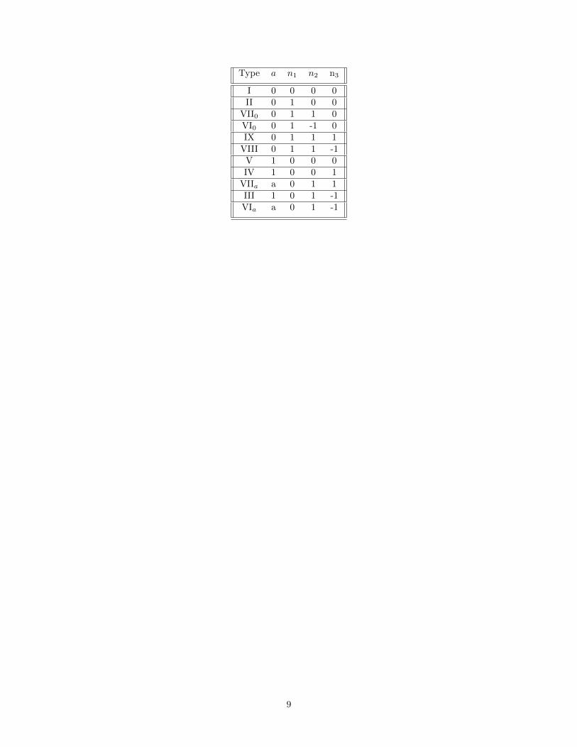
Type a n1 n2 n3

I 0 0 0 0II 0 1 0 0

VII0 0 1 1 0VI0 0 1 -1 0IX 0 1 1 1

VIII 0 1 1 -1V 1 0 0 0IV 1 0 0 1

VIIa a 0 1 1III 1 0 1 -1VIa a 0 1 -1

9

Chapter 3

Poisson Geometry and Dynamics

Our next goal is to provide a geometric framework for understanding Hamiltonian mechanics in terms ofsymplectic and Poisson manifolds. In particular, we will use these objects to study geometric analogues ofDynamics and Equations of Motions; an interpretation of Noether’s theorem using momentum mappings willbe developed in the next chapter. In this essay, we will explore symplectic manifolds as a complementarystructure to the Poisson manifold. Not only will we see that Poisson geometry will allow us to generalisefurther the idea of Hamiltonian dynamics on a symplectic, but we will also see that a Symplectic structure willinduce a Poisson structure which will be of paramount importance since we can define a natural symplecticstructure on the cotangent bundle T ∗G of a Lie group G. In Chapter 4 we will use the induced Poissonstructure to show that the reduced phase space T ∗G/G is isomorphic as a Poisson manifold to the Lie-Poissonstructure on g∗.

3.1 Symplectic Manifolds

Definition 3.1. A symplectic manifold (M,Ω) is a manifold M equipped with a closed nondegeneratetwo-form Ω on M .

The non-degeneracy of Ω means that symplectic manifolds are necessarily even-dimensional; this makessense why we traditionally use symplectic manifolds to generalise Hamiltonian systems as Hamiltonians nec-essarily operate on even dimensional phase space. Presenting dynamics in terms of symplectic manifoldsis the first step of generalising Hamiltonian systems and presents dynamics in terms of the two-form Ω;however, in this essay, we will develop dynamics in terms of Poisson manifolds.

Given two symplectic manifolds (M1,Ω1), (M2,Ω2) we say that a smooth mapping f : M1 → M2 issymplectic if

f∗Ω2 = Ω1, (3.1)

and if f is also a diffeomorphism we call it a symplectomorphism.

Example 3.2 (Cotangent Bundle). We now wish to show that the cotangent bundle of a manifold naturallyinherits a symplectic structure. Let M be a manifold, then we can define a one-form Φ on the cotangentbundle T ∗M as

Φα(f) := 〈α, dπMx〉, (3.2)

where α ∈ T ∗M , x ∈ Tα(T ∗M), πM : T ∗M → M is the natural projection and dπM : T (T ∗M) → TM isthe tangent map of πM . After some algebra one can verify that (T ∗M,Ω := −dΦ) is a symplectic manifold.If we treat our manifold M as the configuration space of a mechanical system then the cotangent bundlecan be thought of as the phase space of the system, on which we expect to be able to define Hamiltoniandynamics, and so it makes sense for it to inherit a symplectic structure.

10

We conclude this brief section by stating a powerful theorem (Darboux’s) for symplectic manifolds, theproof of which can be found in [2, p.149]. Darboux’s theorem tells us that there is a coordinate system fora symplectic manifold in which locally the manifold looks like the phase space of a mechanical system.

Theorem 3.3 (Darboux’s Theorem). If (M,Ω) is a finite-dimensional symplectic manifold then M nec-essarily has dimension dimM = 2n for n ∈ N. Moreover, for each x ∈ M there exist local coordinates(q1, ..., qn, p1, ..., pn) such that the symplectic form in these coordinates is

Ω = dqi ∧ dpi. (3.3)

3.2 Poisson Manifolds

Poisson manifolds will generalise Symplectic geometry and the Poisson bracket for a classical mechanicalsystem; accordingly will provide us with a more generalised understanding of dynamics.

Definition 3.4. A Poisson manifold is a manifold M equipped with a Poisson bracket (also called Poissonstructure), namely a bilinear map , on C∞(M) such that:

• (C∞(M), , ) is a Lie algebra.

• For each f, g, h ∈ C∞(M) we have the derivation property in the first factor: fg, h = f, hg+fg, hand similarly with the second factor.

Similarly to the symplectic case, given two Poisson manifolds (M1, , 1), (M2, , 2), we say that a smoothmapping f : M1 →M2 is a Poisson map if

f∗F,G2 = F,G1, (3.4)

for any F,G ∈ C∞(M).

We can express the Poisson bracket in local coordinates (x1, ..., xn) as

F,G =

n∑i,j=1

xij∂F

∂xi

∂G

∂xj, (3.5)

where xij := xi, xj is called the Poisson matrix in these coordinates.

Consider a Poisson manifold M and the map G 7→ G,H for H,G ∈ C∞(M). By the derivationproperties of the Poisson bracket on M it is clear this map is a derivation on C∞(M). It is a well-knownresult of differential geometry that such derivations are in one to one correspondence with vector fields onM . Thus for H ∈ C∞(M) we can define a unique vector field

XH(G) := G,H, (3.6)

called the Hamiltonian vector field associated with H.

Example 3.5 (Poisson Structure from Symplectic). If (M,Ω) be a symplectic manifold then it is also aPoisson manifold when equipped with the bracket

F,G(x) := Ω(XF [x], XG[x]), (3.7)

where F,G : M → R are smooth functions and x ∈M . Indeed the bilinearity follows from the bilinearity oftwo-forms. Moreover we have

XFG = FXG +GXF , (3.8)

giving us the derivation property:

FG,H = XH [FG] = FXH [G] +GXH [F ] = FG,H+GF,H. (3.9)

11

In this essay we will analyse the Lie-Poisson Structure. Let g be a Lie algebra; then we can define aPoisson structure on its dual g∗ as follows. Let e1, ..., en be a basis for g and recall that we can write thecommutator relations as

[ei, ej ] = fkijek, fkij ∈ R. (3.10)

Let e1, ..., en be the basis of g∗ dual to e1, ..., en, defined as ei := e∗i , where for X = αiei ∈ g we have

e∗i (X) = 〈X, ei〉 := αi. Throughout let µ = xiei, we claim that, for F,G ∈ C∞(g∗), the bilinear map

F,G(µ) = xij∂F

∂xi

∂G

∂xj, (3.11)

is a Poisson structure on C∞(g∗), where xij = [ei, ej ]∗ is the Poisson matrix. Unless confusion arises we will

usually drop the µ dependence in F,G(µ). The bilinearity and derivation property of the Poisson bracketarises from the linearity and derivation properties of partial derivatives. The Jacobi identity and derivationproperty follow after observing e∗k, e∗l = xij∂ie

∗k∂je

∗l = [ek, el]

∗ and by the bilinearity of the bracket thisimplies ξ∗, γ∗ = [ξ, γ]∗ for γ, ξ ∈ g. From here it is obvious that

xi, xj, xk = [[ei, ej ], ek]∗.

Thus the Jacobi identity follows immediately from that of the Lie bracket.

To find a coordinate-free expression of (3.11), given µ ∈ g∗ and F ∈ C∞(g∗); the push forward F∗ :Tµ(g∗) → R can be regarded as an element of g. Indeed g∗ as a vector space is naturally isomorphic toits tangent space Tµ(g∗), thus the push forward can be considered as an element of (g∗)∗, which itself isnaturally isomorphic to g. Hence we identify the push forward at µ ∈ g∗ with an element dµF ∈ g. We canwrite this in terms of the basis as dµF =

∑ni=1

∂F∂xi

(µ)ei.Finally, we state our definition:

Definition 3.6. Let g be a finite-dimensional Lie algebra. The Lie-Poisson bracket (or Lie-Poisson structure)is the Poisson bracket on C∞(g∗):

F,G(µ) :=⟨µ, [dµF, dµG]

⟩, F,G ∈ C∞(g∗), µ ∈ g∗ (3.12)

equipping g∗ with a Poisson manifold structure. Here dµF, dµG are elements of g as just explained.

In the coordinate expression (3.11) we can find xij explicitly:

xij = xi, xj = [ei, ej ]∗,

[ei, ej ]∗ = (fkijek)∗ = fkije

∗k = fkijxk.

Thus Equation (3.11) reduces to:

F,G =

n∑i,j=1

fkijxk∂F

∂xi

∂G

∂xj. (3.13)

Example 3.7. When g is one of the Bianchi Lie algebras from Equations (2.24) we have that the onlynonzero structure constants are:

f212 = a, f312 = n3,

f123 = n1, (3.14)

f231 = n2, f331 = −a.

For this case Equation (3.11) becomes:

F,G = x1(f123(∂2F∂3G− ∂3F∂2G))

+x2(f212(∂1F∂2G− ∂2F∂1G) + f231(∂3F∂1G− ∂1F∂3G)) (3.15)

+x3(f312(∂1F∂2G− ∂2F∂1G) + f331(∂3F∂1G− ∂1F∂3G)),

12

and substituting (3.14) gives us:

F,G = x1(n1(∂2F∂3G− ∂3F∂2G))

+x2(a(∂1F∂2G− ∂2F∂1G) + n2(∂3F∂1G− ∂1F∂3G)) (3.16)

+x3(n3(∂1F∂2G− ∂2F∂1G)− a(∂3F∂1G− ∂1F∂3G)),

for any F,G ∈ C∞(g∗).

3.3 Poisson Dynamics

As we alluded to before, Poisson geometry will generalise the idea of Hamiltonian dynamics for a classicalmechanical system. We now aim to further this by analysing the equations of motion in terms of the Poissonbracket and consider invariants of motion.

Before looking at dynamics we show one important property of Hamiltonian vector fields.

Lemma 3.8. Let M be a Poisson manifold and H,G ∈ C∞(M). We have:

[XH , XG] = −XH,G. (3.17)

Proof.

[XH , XG][F ] = XH [XG[F ]]−XG[XH [F ]]

= F,G, H − F,H, G= −F, G,H (Jacobi)

= −XH,G[F ].

(3.18)

We now look at the main theorem about equations of motion on a Poisson manifold.

Theorem 3.9. Let φt be the flow on a Poisson manifold M of a Hamiltonian vector field XH , whereH : M → R be a smooth function.

1. For F ∈ C∞(U), where U ⊂M is open, we have

d

dt(F φt) = F,H φt = F φt, H. (3.19)

Or in other words, F = F,H for all F ∈ C∞(U) iff φt is the flow of XH .

2. If φt is the flow of XH then H φt = H.

Proof. Let x ∈M .

1. By the chain rule the left hand side becomes:

d

dtF (φt(x)) = dF

∣∣φt(x)

d

dtφt(x).

The right hand side is:F,H

∣∣φt(x)

= dF∣∣φt(x)

XH [φt(x)]

and it follows from the Hahn Banach theorem [12, Theorem 1.1.2, pp. 4-7] that these are equal in anopen set U ⊂M for any F ∈ C∞(M) iff XH [φt(x)] = d

dtφt(x) i.e φt is the flow of XH with initial pointx. Conversely if φt is a flow so that

XH [φt(x)] = (φt)∗(XH [x]),

13

using the chain rule again we see:

d

dtF (φt(x)) = dF

∣∣φt(x)

XH [φt(x)]

= dF∣∣φt(x)

(φt)∗(XH [x])

= d((F φt)(x)XH [x]

= F φt, H(x).

(3.20)

2. Follows from 1. using H = F .

We want to compare the local dynamical equations of due to both Symplectic and Poisson geometry. Inthe Symplectic case, we have local coordinates (by Darboux’s theorem) x := (q1, ..., qn, p1, ..., pn) and theHamiltonian equations of motion will read

~x = J∇H, (3.21)

where J:= [0 In−In 0

]. (3.22)

We compare this to the local Poisson manifold equations of motion. Let (x1, ..., xn) be local coordinates,where n can be either even or odd (as opposed to the symplectic case). If we let Λ be the Poisson matrix inthese coordinates, the dynamical equations xi = H,xi become

~x = Λ∇H. (3.23)

Thus we can see the similarities between the two formulations. However, we stress that the Poisson structureallows for dynamics on a space of arbitrary dimension.

Definition 3.10. Let C ∈ C∞(U) for some open subset, U ⊂M , of a Poisson manifold M. We say that Cis a Casimir function of the Poisson structure if for all H ∈ C∞(M) we have

H,C = 0. (3.24)

An important Corollary of Theorem 3.9 is that if G,H ∈ C∞(M), then G is constant along the integralcurves of XH iff G,H = 0. The Casimir functions are those which have trivial dynamics, that is C will beconstant along the flow of all Hamiltonian vector fields. We note that functions G which are constant alongintegral curves of XH will be the central focus of Chapter 4.

We finish by showing that for any choice in Hamiltonian, the dynamics of the system will live on a levelset of the Casimir function C. Indeed, by the skew-symmetry of the Poisson bracket, we have C,C = 0and so C is constant along the integral curves of XC . Let f, g ∈ C∞(M), using the Jacobi equation we see

C, f, g = f, C, g − g, H, f = 0, (3.25)

where the terms on the right-hand side are zero by definition of a Casimir function; and so C, f, g = 0and the dynamics are restricted to level sets of C.

”Thus for any choice of a Hamiltonian, the resulting dynamics will be constrained to live on a set onwhich L is constant.”

14

3.4 Equations of Motion for g∗

We want to now consider what the equations of motion and Hamiltonian vector fields for a HamiltonianH ∈ C∞(g∗) look like in terms of the Lie-Poisson bracket. Recall the definition of the Lie-Poisson bracketin Equation (3.12) and let F ∈ C∞(g∗). We have

F,H(µ) = 〈µ, [dµF, dµH]〉= 〈µ,−addµHdµF 〉= −〈ad∗dµHµ, dµF 〉.

(3.26)

Moreover by the chain rule we have

dF

dt= dF (µ)

dµ

dt= 〈dµ

dt, dµF 〉 (3.27)

and non-degeneracy of the pairing implies that the equations of motion are

dµ

dt= −ad∗dµHµ. (3.28)

Thus we have that the Hamiltonian vector fields of the Lie-Poisson structure are of the form

XH [µ] = −ad∗dµHµ, (3.29)

for a Hamiltonian H.

Using Equation (3.13) we can write a coordinate expression for the equations of motion:

dF

dt=

n∑i,j=1

fkijxk∂F

∂xi

∂H

∂xj. (3.30)

The problem is too general to solve for any sort of dynamics other than the trivial dynamics in this essay.So we will turn our attention to finding Casimir functions of the Lie-Poisson structure. A Casimir function

of the Lie Poisson structure will satisfy:

XC [F ] =

n∑i,j=1

fkijxk∂F

∂xi

∂C

∂xj= 0, ∀F ∈ C∞(M). (3.31)

In particular for F = xl, l = 1, ..., n we must still have xl, C = 0. This gives us

XC [xl] =

n∑i,j=1

fkijxkδli

∂C

∂xj= 0, (3.32)

=⇒ XC [xl] =

n∑j=1

fkljxkδli

∂C

∂xj= 0, l = 1, ..., n. (3.33)

This will give us a system of n partial differential equations which we hope to solve for a Casimir functionC on some open set U ⊂M . We now look at the specific case of the Bianchi Lie algebras.

Example 3.11. For the Bianchi Lie algebras, using Equation (3.16) we deduce that if C is a Casimirfunction we must have:

(ax2 + n3x3)∂C

∂x2+ (ax3 − n2x2)

∂C

∂x3= 0,

−(ax2 + n3x3)∂C

∂x1+ n1x1

∂C

∂x3= 0, (3.34)

−(ax3 − n2x2)∂C

∂x1− n1x1

∂C

∂x2= 0.

Identifying g∗ ≡ R3 with basis (x2, x2, x3) I found in [8] open sets and Casimir functions for each BianchiLie group as outlined in Table 3.1.

15

Table 3.1: Casimir/Coadjoint Invariant Functions of the Bianchi Groups.

Type Invariant Open Set 0-D Orbits

I 0 R3 EverywhereII x1 R3 − x1 = 0 x1 = 0

VII0 x21 + x22 R3 − x3 axis x3 axisVI0 x21 − x22 R3 − x3 axis x3 axisIX x21 + x22 + x23 R3 − (0, 0, 0) The origin

VIII x21 + x22 − x23 R3 − (0, 0, 0) The originV x2/x3 R3 − x3 = 0 x1 axis

x3/x2 R3 − x2 = 0IV x3 exp(−x2

x3) R3 − x3 = 0 x1 axis

VIIa (x22 + x23) exp(−2a(arctan(x2

x3))) Cylindrical Coordinates: R3 − (x1, 0, 0) x1 axis

III x2 + x3 R∗ − x2 = x3 x2 = x3

VIa>1 (x2 − x3)(x2 + x3)1+a1−a R3 − x2 + x3 = 0 x1 axis

VIa<1 (x2 − x3)(x2 + x3)1+a1−a R3 − x2 = x3 = 0 x1 axis

For Bianchi g∗, it was completely necessary to use Poisson geometry to describe the mechanics since theconfiguration space (which is isomorphic to R3) is three-dimensional and thus symplectic geometry cannotbe applied.

In the next section, we will see that Poisson manifolds decompose into symplectic manifolds called sym-plectic leaves. For the Lie-Poisson bracket the symplectic leaves are coadjoint orbits. Moreover, I showedin [8] that under certain conditions the level sets of the Casimir functions on an open subset of g∗ are thesymplectic leaves themselves. The above table gives a partially complete classification for the coadjointorbits of each Bianchi group.

While dynamics on our manifold cannot be described by Symplectic geometry, it does foliate into sym-plectic manifolds which can be described by level sets of the Casimir functions which are invariant under allHamiltonian vector fields. In fact, our Poisson structure restricted to a leaf is exactly the symplectic form;a proof of this fact can be found in [4]. By our reasoning at the end of the previous section, the dynamicsare restricted to the level sets of the Casimir functions, which are symplectic leaves and thus symplecticmanifolds.

3.5 Symplectic Foliation

We have mentioned how Poisson manifolds will decompose into symplectic manifolds called ’symplecticleaves’ and we next want to give a brief overview of the Theorems used to show this and apply them to theLie-Poisson structure.

At the end of the previous section, we discussed how the dynamics on the Poisson manifold will be re-stricted to the level sets of the Casimir functions. We will see that under certain conditions the level sets ofCasimir functions are exactly the symplectic leaves, and so the Poisson manifold will decompose into levelsets of its Casimir functions.

To motivate this we state without proof the following theorems on the symplectic foliation of a Poissonmanifold, the proofs of which can be found in [4, Section 5.3].

Theorem 3.12. Let M be a Poisson manifold. Then M is the disjoint union of immersed submanifolds

16

whose tangent spaces are spanned by its Hamiltonian vector fields. These submanifolds are symplectic man-ifolds called symplectic leaves. We call the decomposition the symplectic foliation of M .

Theorem 3.13. A function on a Poisson manifold M is a Casimir function if and only if F is constant oneach symplectic leaf.

These two theorems tell us that given a Poisson manifold M , it decomposes into the union of symplecticmanifolds where the Poisson structure restricted to a symplectic leaf is the symplectic form. In fact, Theorem3.13 goes further, which is explained in the following theorem, the proof of which can also be found in [5,Ch. 3].

Theorem 3.14. Let M be a Poisson manifold of dimension n and let U be a nonempty open subset. LetF1, ..., Fr ∈ C∞(U) be such that:

1. The rank of the Poisson matrix is constant of U and equal to n− r.

2. The functions F1, ..., Fr are Casimir functions of the restriction of the Poisson structure to U .

3. For each point ξ of U the differentials (dFi)ξ are independent.

Then the symplectic leaves on U are the level sets of the map (F1, ..., Fr) : U → Rr.

Symplectic foliation thus provides a beautiful connection between the two types of manifolds we havediscussed in this essay. Now we wish to show that for the Lie-Poisson bracket the symplectic leaves areexactly the coadjoint orbits and the Casimir functions are the coadjoint invariant functions.

Let G be a connected Lie group (hence why we defined the Bianchi groups as being connected) whoseLie algebra is g. We show that the set of infinitesimal generators of the coadjoint action coincides with theset of Hamiltonian vector fields on g∗, so that we can apply Theorem 3.12. In Equation (3.29) we showedthat the Hamiltonian vector fields were

XH [µ] = −ad∗dµHµ, (3.35)

for µ ∈ g∗ and a Hamiltonian H. Now for ξ ∈ g we have dµξ∗ = ξ∗ where ξ∗ := 〈µ, ξ〉. Thus it follows that

the set of Hamiltonian vector fields at µ ∈ g∗ is

ad∗dµFµ : F ∈ C∞(g∗) = ad∗ξµ : ξ ∈ g, (3.36)

which gives us our result after realising that G being connected means the coadjoint orbits are connectedand so the symplectic leaves are coadjoint orbits by Theorem 3.12.Moreover, it follows from Theorem 3.13 that the Casimir functions of the Lie-Poisson bracket are thosethat are constant on symplectic leaves, i.e. Ad∗ invariant functions. In [8] I showed that for the BianchiLie groups; we could apply Theorem 3.14to show that the symplectic leaves were level sets of the Casimirfunctions we found.

17

Chapter 4

Momentum Maps and Noether’sTheorem

We now aim to use the theory of Poisson geometry as developed in the previous chapter to provide ageometric understanding of Noether’s theorem. A usual first course in the Lagrangian and Hamiltonianformulation of Classical Mechanics will introduce aspiring physicists to the notion of how symmetries giverise to conserved quantities via Noether’s theorem. First examples are usually symmetry of time translation,which implies conservation of energy; symmetry under rotation gives conservation of angular momentum;translational symmetry implies conservation of momentum; a reference for these derivations can be found in[6]. Our geometric generalisation of conserved quantities arising from symmetries will be realised throughthe momentum map.

4.1 Momentum Maps

We begin by recalling that if Φg is a left action of a Lie group G on a manifold M then for each g ∈ G themap Φg : M →M is a smooth map. Furthermore, if M is a Poisson manifold and if for each g ∈ G we havethat Φg is a Poisson map, i.e.

Φ∗gF,G = Φ∗gF,Φ∗gG, (4.1)

for any F,G ∈ C∞(M): then we say that the action is a Poisson action. Let ξ ∈ g; then differentiating (4.1)in the direction of ξ we get:

d

dt(exp(tξ)F,G)

∣∣t=0

= ddt

(exp(tξ)F )∣∣t=0

, G+ F, ddt

(exp(tξ)G)∣∣t=0. (4.2)

Recalling from Equation (2.8) the definition of the infinitesimal action we have:

ξF,G = ξF,G+ F, ξG; (4.3)

in this case, we say that the action is an infinitesimal Poisson automorphism.

However we are interested in a slightly stronger condition: namely, that there exists a global HamiltonianJ(ξ) ∈ C∞(M) for the infinitesimal action ξ, i.e:

XJ(ξ) = ξ. (4.4)

We will say that a Lie algebra acts canonically on a Poisson manifold if (4.4) is satisfied. We are now readyto define a momentum map.

Definition 4.1. Let g be a Lie algebra which acts canonically on a Poisson manifold M . Suppose that thereis a linear map J : g→ C∞(M) such that J satisfies (4.4) for all ξ ∈ g. The map

J : M → g∗

18

〈J(x), ξ〉 := J(ξ)(x), (4.5)

for ξ ∈ g and x ∈M is called a momentum map of the action.

As we alluded to before; if we have symmetries arising from the action of our Lie group we hope to beable to mirror Noether’s theorem by finding such a momentum map that will correspond to a conservedquantity of the symmetry.

Returning to the Lie-Poisson structure, we want a map J : g→ C∞(g∗) such that J satisfies (4.4) for allξ ∈ g. We first show that the coadjoint action is a Poisson action. Indeed given F,G ∈ C∞(g∗) and lettingα = Ad∗g−1 we have

F,G(αµ) = 〈αµ, [dαµF, dαµG]〉= 〈αµ, [Adgdµ(F α), Adgdµ(G α)]〉= 〈µ, [dµ(F α), dµ(G α)]〉= F α,G α(µ);

(4.6)

where in the second line we used the identity:

dαF = Adgdµ(F α). (4.7)

Now for the coadjoint action the infinitesimal acition is

ξ =d

dt(exp(tξ)µ)

∣∣t=0

= −ad∗ξµ, (4.8)

for µ ∈ g∗ and ξ ∈ g. Thus (4.4) in this case becomes:

ad∗dµJ(ξ)µ = ad∗ξµ. (4.9)

Hence the momentum map is the identity on g∗, which we see after realising

J(ξ)(µ) = 〈µ, ξ〉. (4.10)

While in some sense this result is trivial, it will allow us to later classify the allowable Hamiltonians for theLie-Poisson bracket and show that the dynamics must be generated by Casimir functions.

4.2 Noether’s Theorem

As promised, we are now going to provide a geometric interpretation of Noether’s theorem for Poissonmanifolds. Let g act canonically on a Poisson manifold M and assume there exists a momentum mapJ : M → g∗. Let H ∈ C∞(M) be a g− invariant Hamiltonian, that is

ξ(H) = 0, ∀ξ ∈ g, (4.11)

which tells us that J(ξ), H = 0. Thus for any ξ ∈ g it follows that J(ξ) is conserved along the flow ofXH , the Hamiltonian vector field associated with H. Thus J is conserved. We have proved the followingTheorem:

Theorem 4.2 (Noether’s Theorem). Let g act canonically on the Poisson manifold M and assume thereexists a momentum map J : M → g∗. If H ∈ C∞(M) is g−invariant for all ξ ∈ g then

J φt = J, (4.12)

where φt is the flow of XH . I.e. J is a constant of motion. If the Lie algebra action comes from a Poissonaction Φg of G then the invariance hypothesis of H is automatically satisfied.

19

As we hoped, we have a version of Noether’s theorem which tells us that if an action preserves the Poissonstructure on a Poisson manifold, then if there exists a momentum map it is a constant of motion. FromClassical Mechanics courses, we know that translation invariance should imply that linear momentum isconserved; so we hope that our version of Noether’s theorem will describe the same result.Indeed, let us consider an n particle system and let R3n act on T ∗R3n ∼= R6n via the action

~x(~qi, ~pi) := (~qi + ~x, ~pi). (4.13)

For Noether’s theorem to be applied we need this to be a canonical action, i.e. Equation (4.4) must besatisfied. First we note that if ξ ∈ g then differentiating the action tells us our infinitesimal action is

ξ(~qi, ~pi) = (ξ, ..., ξ, 0, ..., 0); (4.14)

and so applying Equation (4.4) we find

XJ(ξ)(~qi, ~pi) = (

∂J(ξ)

∂~pi,−∂J(ξ)

∂~qi) = (ξ, ..., ξ, 0, ..., 0). (4.15)

Thus, it follows that

J(ξ)(~qi, ~pi) = (

n∑i=1

~pi)ξ, (4.16)

and so the momentum map is exactly the linear momentum

J(~qi, ~pi) = (

n∑i=1

~pi), (4.17)

which will be a constant of motion along any g−invariant Hamiltonian, as we expect.

4.3 Noether’s Theorem on g∗

We will now apply Noether’s theorem to the Lie-Poisson structure of the dual Lie algebras g∗, to find thepossible Hamiltonians on g∗. In some sense the resulting dynamics will be trivial, however, it will allow usto express the tools we have developed thus far in this essay. We will then be able to classify the possibleHamiltonians in the Bianchi case and show that they are the Casimir functions we found before — recallingfrom Section 3.4 that the dynamics are restricted to level sets of these Casimir functions.

From Equation (4.10) we recall that J = Idg∗ is a momentum map for the Lie-Poisson bracket on g∗.Moreover the derivation in Equations (4.6) showed us that the coadjoint action of G was Poisson. It followsthat for any g−invariant Hamiltonian H ∈ C∞(g∗) we must have, by Equation (4.12), that

Idg∗ φt = Idg∗ , (4.18)

where φt is the flow of XH . In other words the flow of the Hamiltonian vector field must be the identity.Equation (4.18) tells us that

d

dtφt(x) = XH(φt(x)) = 0, (4.19)

and recalling from Equation 3.31 the form of the Hamiltonian vector fields of the Lie-Poisson bracket in ourusual basis for g∗:

XH [φt(x1, ..., xn)] =

n∑i,j=1

fkijxk∂(x1, ..., xn)

∂xi

∂H

∂xj=

n∑i,j=1

fkijxk∂H

∂xj= 0; (4.20)

and so we must haven∑

i,j=1

fkijxk∂H

∂xj= 0. (4.21)

20

Example 4.3. Specializing to the Bianchi Lie groups, we stated in Equation (3.14) the structure constantsof the Bianchi Lie algebras; from here it follows that a Hamiltonian on a Bianchi g∗, HB , must satisfy

∂HB

∂x1(−ax2 − n3x3 + n2x2 − ax3) +

∂HB

∂x2(ax2 + n3x3 − n1x1) +

∂HB

∂x3(n1x1 + ax3 − n2x2) = 0. (4.22)

It is easy to check that the Casimir functions we defined in Table 3.1 solve this.

Returning to the general case of the Lie-Poisson bracket take our coadjoint invariant functions (Casimirfunctions) and analyse which ones solve (4.21). If we recall from Section 2.3, Casimir functions generatetrivial dynamics on g∗, that is they are constant along the flow of all Hamiltonian vector fields; in fact, wewill show that the only dynamics on g∗ are trivial.

To classify the dynamics on g∗ and show that the only allowable Hamiltonians applicable to Noether’stheorem are the Casimir functions, we recall from Section 3.4 that the Ad∗ invariant functions are theCasimir functions and so that to apply Noether’s theorem we must have that the Hamiltonian is a Casimirfunction. Theorem 3.13 tells us for the Lie-Poisson bracket the Hamiltonians which can be applied toNoether’s Theorem are exactly the Casimir functions, provided the Lie group G is connected. Thus thedynamics on g∗ must be trivial.

Example 4.4. For the Bianchi Lie groups, which we defined as being simply connected and connected,we were able to provide a classification of the Casimir functions on open subsets of g∗, thus we have beenable to entirely classify the trivial dynamics of the Lie-Poisson structure of the Bianchi Lie-groups andso we have classified the dynamics of the reduced phase space T ∗G/G for a three-dimensional space whichadmits a continuous group of motions. Thus we have classified Hamiltonian dynamics on a three-dimensionalconfiguration space, a task that Poisson geometry was necessary to do.

21

Chapter 5

Reduction

Our final chapter is a technical one to show that the canonical Poisson bracket on the cotangent space T ∗Gis related to the Lie-Poisson bracket we defined on g∗. Some of the technical aspects of the theory we developwill be based on bundle theory and the proofs shall be omitted but may be found in [2]. Our proof of theLie-Poisson Reduction theorem will use the fact that we have derived the Lie-Poisson bracket on g∗ already;a more constructive proof without assuming this can be found in [4].

5.1 Lie-Poisson Reduction

We now aim to prove the following theorem, which states that the reduced phase space of a Lie group T ∗G/Gis a Poisson manifold diffeomorphic to the Lie algebra g = TeG. Throughout the section, the subscript onthe bracket indicates the space in which the bracket is defined.

We first introduce some notation, namely for αg ∈ T ∗gG define O(αg) to be the set

O(αg) := β ∈ T ∗G : β = T ∗Rg−1(α), for some g ∈ G. (5.1)

Theorem 5.1 (Lie-Poisson Reduction Theorem). Suppose αg ∈ T ∗G, the map

f : T ∗G/G→ g∗ (5.2)

O(αg) 7→ T ∗eRg(α),

is both a diffeomorphism and a Poisson map.

The proof that f : T ∗G/G → g∗ is a diffeomorphism requires bundle theory so we will provide only abrief overview of the proof. We can see this by considering the map

λ : T ∗gG→ G× g∗, (5.3)

λ(αg) := (g, T ∗eRg(αg)),

which transforms the cotangent lift of the right action on G into the action of G on G× g∗ given by

g(h, ξ) ≡ Φg(h, ξ) := (gh, ξ), (5.4)

and so we have the following diffeomorphisms:

T ∗G/G ∼= (G× g∗)/G ∼= g∗. (5.5)

Thus we have the desired diffeomorphism T ∗G/G ∼= g∗.Now the map f : T ∗G/G→ g∗ provides us with the commutative triangle:

T ∗G/G

T ∗G g∗

fπ

JL

22

where π is the canonical projection and JL := T ∗e Lg is the momentum map of the cotangent lift of righttranslation on G; so that JL = f π. We note that because Rg : G→ G is a diffeomorphism then it can beshown that its cotangent lift is a symplectic map.

We claim that if Φg is a Poisson action (cf. Equation (4.1)) of G on a Poisson manifold M then, assumingM/G is well defined and π : M →M/G is a smooth submersion, there exists a unique Poisson structure onM/G such that π is a Poisson map. Indeed, let α : M/G→ R be a smooth real valued function and considerits pull back α := π∗α under π, then α([x]) = π∗α([x]) is well defined as it is constant on G−orbits. Thusfor β, γ : M/G→ R we have

β, γM/G π = β π, β πM ≡ β, γM , (5.6)

because π is a Poisson map. Moreover the surjectivity of π tells us that β, γ is determined uniquely. Nowrecalling that Φg is a Poisson action and the pull backs of β and γ under π are constant on G−orbits wehave

β, γ(Φg(x)) = (β, γ Φg(x)

= β Φg, γ Φg(x) (Poisson Action)

= β, γ(x), (Constant on G−orbits)

(5.7)

an so β, γ is also constant on G−orbits; therefore the bracket is well-defined. Moreover, the derivationproperties, bilinearity and Jacobi identity all follow from the bracket on M .

Using this claim it follows that there is a unique Poisson structure on T ∗G/G such that π is a Poissonmap. The map JL = T ∗eRg is a Poisson map because of equivariance (show); it follows the map f is Poisson,meaning

(F,Gg∗ f)(x) = F f,H fT∗G/G(x), (5.8)

for F,G ∈ C∞(g∗) and x ∈ T ∗G/G.

To finish the proof, we note that because π is surjective, there exists an αg ∈ T ∗G for each x ∈ T ∗G/Gsuch that x = π(αg). Moreover recall that JL = f π is a Poisson map. It follows that

(F,Hg∗ f)(x) = F f,H fg∗(f π)(αg)

= F,Hg∗ JL(αg)

= F JL, H JLT∗G(αg)

= F f,H fT∗G/G(π(αg))

= F f,H fT∗G/G(x).

(5.9)

23

Chapter 6

Conclusion

6.1 Concluding Remarks

Throughout this essay, we aimed to show the power of Poisson geometry by defining dynamics on a manifoldof arbitrary dimension and readily applying it to the case of the Lie-Poisson structure. We found that thedynamics of Poisson geometry were constrained to live on the level sets of the Casimir functions and proved ageometric version of Noether’s theorem. Our development of the theory allowed us to understand symmetriesof Hamiltonian systems and we applied this to the case of the Bianchi g∗, a three-dimensional Poissonmanifold and showed that the Hamiltonian dynamics were trivial. Moreover, we related the symplecticfoliation of g∗ to the coadjoint orbits of the corresponding Bianchi group G. We concluded the essay with aproof showing that the reduced phase space T ∗G/G was a Poisson manifold diffeomorphic to g∗.

As a final glimpse into the richness of this subject, Section 6.2 will very briefly discuss its relation toquantum theory.

6.2 Glimpsping Further Developments: Geometric Quantizationand the Orbit Method

Quantization refers to the process of taking a classical mechanical system and translating it into a quantumanalogue by mapping classical observables to quantum operators. When considering a classical system whosephase space is described by a symplectic manifold (M,Ω), geometric quantization aims to quantize M byconstructing a map sending observables f ∈ C∞(M) to operators on a Hilbert space H:

Q : C∞(M)→ Op(H). (6.1)

Dirac proposed certain conditions which such a map should obey; perhaps unsurprisingly, these are knownas the Dirac quantization conditions:

1. The map Q must be linear on C∞(M).

2. The map must relate commutators to Poisson brackets in the following sense:

[Q(f), Q(g)] = −i~Q(f, g). (6.2)

3. Constant observables must get mapped to constant operators:

Q(f) = fI, (6.3)

for f constant.

4. Completeness: if fi form a complete set of observables for the classical system then Q(fi) form acomplete set of operators for the quantum system.

24

The exact formulation of geometric quantization is described in [10]. However, the theory of geometricquantization involves understanding line bundles, this would provide content enough for another Part IIIessay in itself.

In summary: geometric quantization amounts to a two-step process known as pre-quantization andpolarization. A pre-quantization on a symplectic manifold (M,Ω) is a complex line bundle B over Mtogether with a connection ∇ and a Hilbert structure H on the line bundle. Here the quantization map isdefined as

Q(f) := −i∇Xf + f. (6.4)

Pre-quantization does a good job at mapping observables to operators. However, we must reduce this toa smaller space so that Condition 4. of the Dirac conditions is met. The process of polarization allows usto do exactly this. We stress that this is an extremely brief overview and invite the reader to explore thetheory of geometric quantization in [10].

In essence, quantization is concerned with finding unitary representations of the structure of the classicalphase space. The Orbit Method, described extensively in [11], concerns itself with finding unitary represen-tations of Lie groups. If we have a Lie group G and know its coadjoint orbits, finding unitary representationsof G amounts to performing geometric quantization on quantizable orbits. Indeed, we know from our workin the previous chapters that coadjoint orbits are symplectic manifolds; so quantization can be well definedon them. The orbit method identifies unitary representations of a Lie group G with the action of G on thestate space of the geometric quantization.

25

Bibliography

[1] Jean-Pierre Serre. Lie Algebras and Lie Groups. Part of the Lecture Notes in Mathematics book series(LNM, volume 1500), Springer, 1992.

[2] Marsden, J.E., Ratiu, Tudor. Introduction to Mechanics and Symmetry. A Basic Exposition of ClassicalMechanical Systems, Springer, 1999.

[3] Bianchi, L. Sugli spazi a tre dimensioni che ammettono un gruppo continuo di movimenti [On three-dimensional spaces which admit a continuous group of motions].Relativity and Gravitation 33, 2171–2253 (2001).https://doi.org/10.1023/A:1015357132699

[4] J. Butterfield On Symplectic Reduction in Classical Mechanics, in J. Earman and J. Butterfield (eds.)The Handbook of Philosophy of Physics, North Holland (2006); 1 - 131. Available at: http://arxiv.org/abs/physics/0507194.

[5] Camille Laurent-Gengoux, Anne Pichereau and Pol VanhaeckePoisson Structures.Springer, 2013.

[6] Arnold, V.I.Mathematical Methods of Classical Mechanics.Springer, 1978.

[7] L.D. Landau and E.M. LifshitzClassical Theory of Fields.Butterworth-Heinemann, 1980.

[8] O’Callaghan, M.Coadjoint Orbits Calculations, Undergrad Research Project, Trinity College, Dublin 2020.

[9] Ado, Igor D. (1935), ”Note on the representation of finite continuous groups by means of linear substi-tutions”, Izv. Fiz.-Mat. Obsch. (Kazan’), 7: 1–43. (Russian language)

[10] Carosso, AGeometric QuantizationDepartment of Physics, University of Colorado, Boulder, Colorado 80309, United States

[11] Kirillov, ALectures on the Orbit MethodAmerican Mathematical Society, 2004.

[12] Kadison, R.V. and Ringrose J.R.Fundamentals of the Theory of Operator Algebras. Volume I: Elementary TheoryAmerican Mathematical Society 1991.

26