Symmetry and Particle Physics

Michaelmas Term 2007

Jan B. GutowskiDAMTP, Centre for Mathematical SciencesUniversity of CambridgeWilberforce Road, CambridgeCB3 0WA, UKEmail: J.B.Gutowski@damtp.cam.ac.uk

Contents

1. Introduction to Symmetry and Particles 51.1 Elementary and Composite Particles 51.2 Interactions 7

1.2.1 The Strong Interaction 71.2.2 Electromagnetic Interactions 81.2.3 The weak interaction 101.2.4 Typical Hadron Lifetimes 12

1.3 Conserved Quantum Numbers 12

2. Elementary Theory of Lie Groups and Lie Algebras 142.1 Differentiable Manifolds 142.2 Lie Groups 142.3 Compact and Connected Lie Groups 162.4 Tangent Vectors 172.5 Vector Fields and Commutators 192.6 Push-Forwards of Vector Fields 212.7 Left-Invariant Vector Fields 212.8 Lie Algebras 232.9 Matrix Lie Algebras 242.10 One Parameter Subgroups 272.11 Exponentiation 292.12 Exponentiation on matrix Lie groups 302.13 Integration on Lie Groups 312.14 Representations of Lie Groups 332.15 Representations of Lie Algebras 372.16 The Baker-Campbell-Hausdorff (BCH) Formula 382.17 The Killing Form and the Casimir Operator 45

3. SU(2) and Isospin 483.1 Lie Algebras of SO(3) and SU(2) 483.2 Relationship between SO(3) and SU(2) 493.3 Irreducible Representations of SU(2) 51

3.3.1 Examples of Low Dimensional Irreducible Representations 543.4 Tensor Product Representations 55

3.4.1 Examples of Tensor Product Decompositions 573.5 SU(2) weight diagrams 583.6 SU(2) in Particle Physics 59

3.6.1 Angular Momentum 593.6.2 Isospin Symmetry 59

– 1 –

3.6.3 Pauli’s Generalized Exclusion Principle and the Deuteron 613.6.4 Pion-Nucleon Scattering and Resonances 61

3.7 The semi-simplicity of (complexified) L(SU(n+ 1)) 63

4. SU(3) and the Quark Model 654.1 Raising and Lowering Operators: The Weight Diagram 66

4.1.1 Triangular Weight Diagrams (I) 694.1.2 Triangular Weight Diagrams (II) 714.1.3 Hexagonal Weight Diagrams 734.1.4 Dimension of Irreducible Representations 774.1.5 The Complex Conjugate Representation 77

4.2 Some Low-Dimensional Irreducible Representations of L(SU(3)) 784.2.1 The Singlet 784.2.2 3-dimensional Representations 784.2.3 Eight-Dimensional Representations 81

4.3 Tensor Product Representations 814.3.1 3⊗ 3 decomposition. 824.3.2 3⊗ 3 decomposition 844.3.3 3⊗ 3⊗ 3 decomposition. 86

4.4 The Quark Model 894.4.1 Meson Multiplets 894.4.2 Baryon Multiplets 904.4.3 Quarks: Flavour and Colour 91

5. Spacetime Symmetry 945.1 The Lorentz Group 945.2 The Lorentz Group and SL(2,C) 975.3 The Lie Algebra L(SO(3, 1)) 995.4 Spinors and Invariant Tensors of SL(2,C) 101

5.4.1 Lorentz and SL(2,C) indices 1025.4.2 The Lie algebra of SL(2,C) 104

5.5 The Poincare Group 1045.5.1 The Poincare Algebra 1055.5.2 Representations of the Poincare Algebra 1065.5.3 Massive Representations of the Poincare Group: kµ = (m, 0, 0, 0) 1115.5.4 Massless Representations of the Poincare Group: kµ = (E,E, 0, 0) 111

6. Gauge Theories 1146.1 Electromagnetism 1146.2 Non-Abelian Gauge Theory 115

6.2.1 The Fundamental Covariant Derivative 1156.2.2 Generic Covariant Derivative 116

6.3 Non-Abelian Yang-Mills Fields 118

– 2 –

6.3.1 The Yang-Mills Action 1196.3.2 The Yang-Mills Equations 1206.3.3 The Bianchi Identity 121

6.4 Yang-Mills Energy-Momentum 1226.5 The QCD Lagrangian 123

– 3 –

Recommended Books

General Particle Physics Books

? D. H. Perkins, Introduction to High energy Physics, 4th ed., CUP (2000).

• B. R. Martin and G. Shaw, Particle Physics, 2nd ed., Wiley (1998).

Lie Algebra books written for Physicists

? H. Georgi, Lie Algebras in Particle Physics, Perseus Books (1999).

? J. Fuchs and C. Schweigert, Symmetries, Lie Algebras and Representations, 2nd ed.,CUP (2003).

• H. F. Jones, Groups, Representations and Physics, 2nd ed., IOP Publishing (1998).

• J. Cornwell, Group Theory in Physics, (Volume 2), Academic Press (1986).

Pure Mathematics Lie Algebra books

• S. Helgason, Differential geometry, Lie groups, and symmetric spaces, 3rd ed., Aca-demic Press (1978).

? H. Samelson, Notes on Lie Algebras, Springer (1990).

• W. Fulton and J. Harris, Representation Theory, A First Course, 3rd ed. Springer(1991).

For an introduction to some aspects of Lie group differential geometry not covered inthis course:

• M. Nakahara, Geometry, Topology and Physics, 2nd ed., Institute of Physics Pub-lishing (2003).

References for Spacetime Symmetry and Gauge Theory Applications

• T-P. Cheng and L-F. Li, Gauge Theory of Elementary Particle Physics, Oxford(1984).

? S. Pokorski, Gauge Field Theories, 2nd ed., CUP (2000).

• S. Weinberg, The Quantum Theory of Fields, (Book 1), CUP (2005).

? J. Buchbinder and S. Kuzenko, Ideas and Methods of Supersymmetry and Supergrav-ity, Or a Walk Through Superspace, 2nd ed., Institute of Physics Publishing (1998).

– 4 –

1. Introduction to Symmetry and Particles

Symmetry simplifies the description of physical phenomena. It plays a particularly impor-tant role in particle physics, for without it there would be no clear understanding of therelationships between particles. Historically, there has been an “explosion” in the numberof particles discovered in high energy experiments since the discovery that atoms are notfundamental particles. Collisions in modern accelerators can produce cascades involvinghundreds of types of different particles: p, n,Π,K,Λ,Σ . . . etc.

The key mathematical framework for symmetry is group theory: symmetry transfor-mations form groups under composition. Although the symmetries of a physical system arenot sufficient to fully describe its behaviour - for that one requires a complete dynamicaltheory - it is possible to use symmetry to find useful constraints. For the physical systemswhich we shall consider, these groups are smooth in the sense that their elements dependsmoothly on a finite number of parameters (called co-ordinates). These groups are Liegroups, whose properties we will investigate in greater detail in the following lectures. Wewill see that the important information needed to describe the properties of Lie groups isencoded in “infinitessimal transformations”, which are close in some sense to the identitytransformation. The properties of these transformations, which are elements of the tangentspace of the Lie group, can be investigated using (relatively) straightforward linear algebra.This simplifies the analysis considerably. We will make these rather vague statements moreprecise in the next chapter.

Examples of symmetries include

i) Spacetime symmetries: these are described by the Poincare group. This is only anapproximate symmetry, because it is broken in the presence of gravity. Gravity is theweakest of all the interactions involving particles, and we will not consider it here.

ii) Internal symmetries of particles. These relate processes involving different typesof particles. For example, isospin relates u and d quarks. Conservation laws can befound for particular types of interaction which constrain the possible outcomes. Thesesymmetries are also approximate; isospin is not exact because there is a (small) massdifference between mu and md. Electromagnetic effects also break the symmetry.

iii) Gauge symmetries. These lead to specific types of dynamical theories describingtypes of particles, and give rise to conserved charges. Gauge symmetries if present,appear to be exact.

1.1 Elementary and Composite Particles

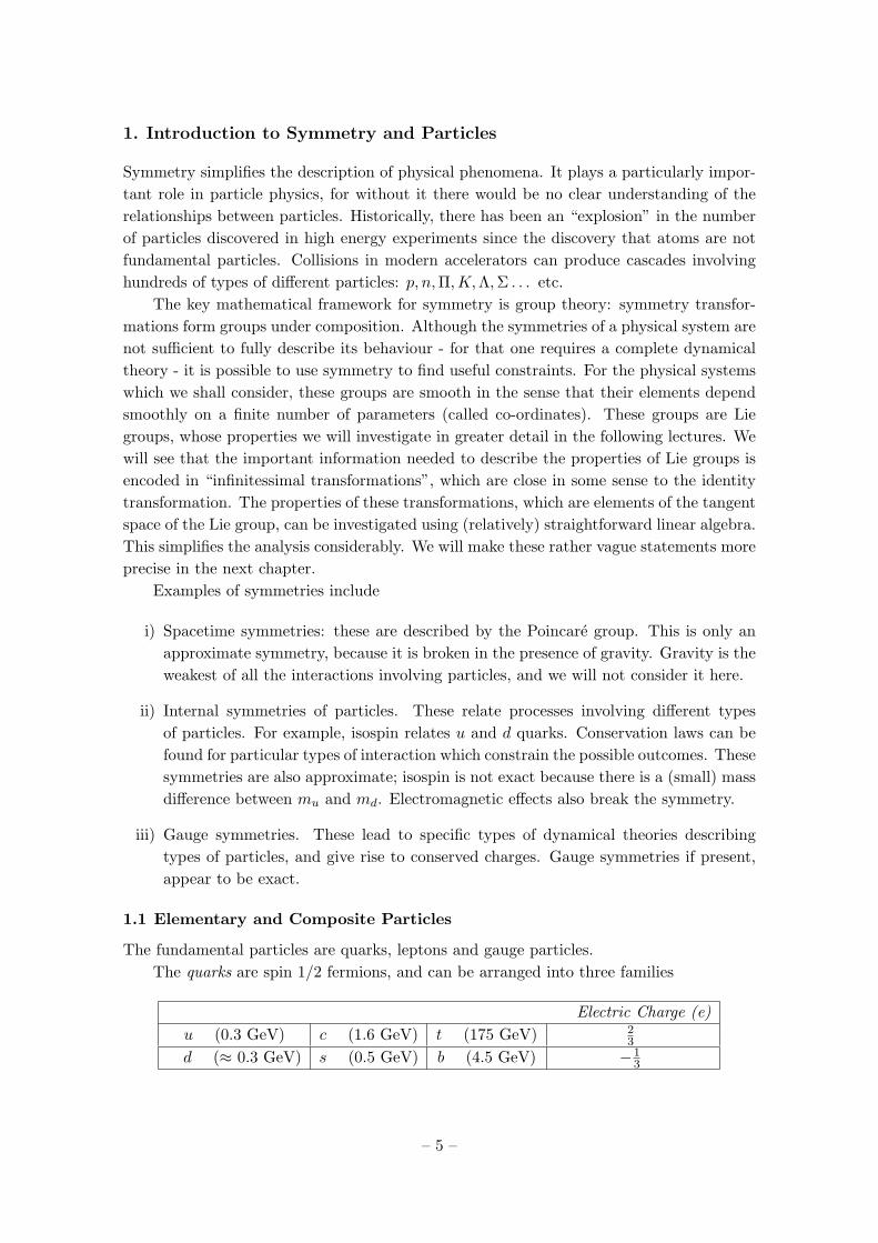
The fundamental particles are quarks, leptons and gauge particles.The quarks are spin 1/2 fermions, and can be arranged into three families

Electric Charge (e)u (0.3 GeV) c (1.6 GeV) t (175 GeV) 2

3

d (≈ 0.3 GeV) s (0.5 GeV) b (4.5 GeV) −13

– 5 –

The quark labels u, d, s, c, t, b stand for up, down, strange, charmed, top and bottom.The quarks carry a fractional electric charge. Each quark has three colour states. Quarksare not seen as free particles, so their masses are ill-defined (the masses above are “effective”masses, deduced from the masses of composite particles containing quarks).

The leptons are also spin 1/2 fermions and can be arranged into three families

Electric Charge (e)e− (0.5 MeV) µ− (106 MeV) τ− (1.8 GeV) −1νe (< 10 eV) νµ (< 0.16 MeV) ντ (< 18 MeV) 0

The leptons carry integral electric charge. The muon µ and taon τ are heavy unstableversions of the electron e. Each flavour of charged lepton is paired with a neutral particleν, called a neutrino. The neutrinos are stable, and have a very small mass (which is takento vanish in the standard model).

All these particles have antiparticles with the same mass and opposite electric charge(conventionally, for many particles, the antiparticles carry a bar above the symbol, e.g.the antiparticle of u is u). The antiparticles of the charged leptons are often denoted bya change of − to +, so the positron e+ is the antiparticle of the electron e− etc. Theantineutrinos ν differ from the neutrinos ν by a change in helicity (to be defined later...).

Hadrons are made from bound states of quarks (which are colour neutral singlets).

i) The baryons are formed from bound states of three quarks qqq; antibaryons are formedfrom bound states of three antiquarks qqq

For example, the nucleons are given by

p = uud : 938 Mev

n = udd : 940 Mev

ii) Mesons are formed from bound states of a quark and an antiquark qq.

For example, the pions are given byπ+ = ud : 140 Mev

π− = du : 140 Mev

π0 = uu, dd superposition : 135 Mev

Other particles are made from heavy quarks; such as the strange particles K+ = us

with mass 494 Mev , Λ = uds with mass 1115 Mev, and Charmonium ψ = cc with mass3.1 Gev.

The gauge particles mediate forces between the hadrons and leptons. They are bosons,with integral spin.

– 6 –

Mass (GeV) Interactionγ (photon) 0 Electromagnetic

W+ 80 WeakW− 80 WeakZ0 91 Weak

g (gluon) 0 Strong

The gluons are responsible for interquark forces which bind quarks together in nucleons.It is conjectured that a spin 2 gauge boson called the graviton is the mediating particlefor gravitational forces, though detecting this is extremely difficult, due to the weakness ofgravitational forces compared to other interactions.

1.2 Interactions

There are three types of interaction which are of importance in particle physics: the strong,electromagnetic and weak interactions.

1.2.1 The Strong Interaction

The strong interaction is the strongest interaction.

• Responsible for binding of quarks to form hadrons (electromagnetic effects are muchweaker)

• Dominant in scattering processes involving just hadrons. For example, pp → pp isan elastic process at low energy; whereas pp −→ ppπ+π− is an inelastic process athigher energy.

• Responsible for binding forces between nucleons p and n, and hence for all nuclearstructure.

Properties of the Strong Interaction:

i) The strong interaction preserves quark flavours, although qq pairs can be producedand destroyed provided q, q are the same flavour.

An example of this is:

d s

Σ+

π+K

+

duu

uu

s

u u

p

– 7 –

The Σ+ and K+ particles decay, but not via the strong interaction, because of con-servation of strange quarks.

ii) Basic strong forces are “flavour blind”. For example, the interquark force betweenqq bound states in the ψ = cc (charmonium) and Υ = bb (bottomonium) mesons arewell-approximated by the potential

V ∼ α

r+ βr (1.1)

and the differences in energy levels for these mesons is approximately the same.

The binding energy differences can be attributed to the mass difference of the b andc quarks.

iii) Physics is unchanged if all particles are replaced by antiparticles.

The dynamical theory governing the strong interactions is Quantum Chromodynamics(QCD), which is a gauge theory of quarks and gluons. This is in good agreement withexperiment, however non-perturbative calculations are difficult.

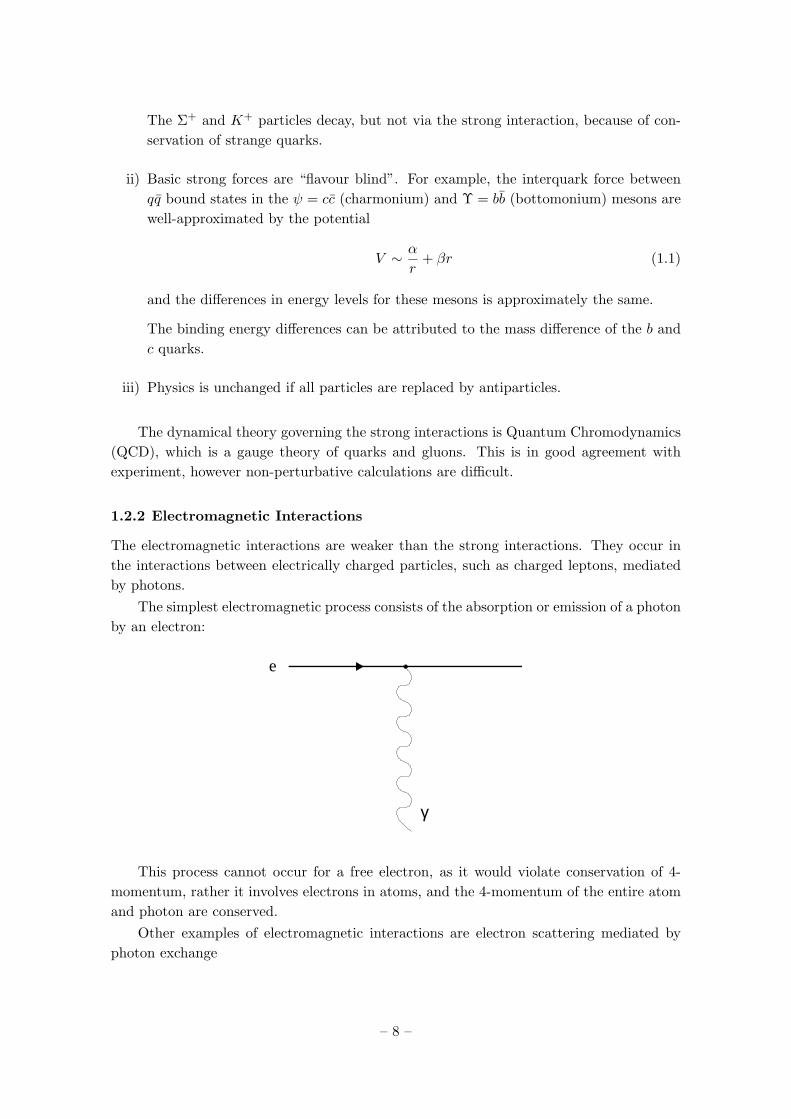
1.2.2 Electromagnetic Interactions

The electromagnetic interactions are weaker than the strong interactions. They occur inthe interactions between electrically charged particles, such as charged leptons, mediatedby photons.

The simplest electromagnetic process consists of the absorption or emission of a photonby an electron:

e

γ

This process cannot occur for a free electron, as it would violate conservation of 4-momentum, rather it involves electrons in atoms, and the 4-momentum of the entire atomand photon are conserved.

Other examples of electromagnetic interactions are electron scattering mediated byphoton exchange

– 8 –

e

e

γ

and there are also smaller contributions to this process from multi-photon exchanges.Electron-positron interactions are also mediated by electromagnetic interactions

e+

e−

e+

e−

γ

e−

e+

e−

e+

γ

+

Electron-positron annihilation can also produce particles such as charmonium or bot-tomonium

e−

e+ HADRONS

γ ψ

– 9 –

The dynamic theory governing electromagnetic interactions is Quantum Electrody-namics (QED), which is very well tested experimentally.

Neutrinos have no electromagnetic or strong interactions.

1.2.3 The weak interaction

The weak interaction is considerably weaker than both the strong and electromagneticinteractions, they are mediated by the charged and neutral vector bosons W± and Z0

which are very massive and produce only short range interactions. Weak interactionsoccur between all quarks and leptons, however they are in general negligable when thereare strong or electromagnetic interactions present. Only in the absence of strong andelectromagnetic interactions is the weak interaction noticable.

Unlike the strong and electromagnetic interactions, weak interactions can involve neu-trinos. Weak interactions, unlike strong interactions, can also produce flavour change inquarks and neutrinos.

The gauge bosons W± carry electric charge and they can change the flavour of quarks.Examples of W -boson mediated weak interactions are n −→ p+ e− + νe:

e−

νe

W−

ddu

udu

n p

and µ− −→ e− + νe + νµ:

– 10 –

W−

e−

νe

µ−

µν

and νµ + n→ µ− + p

νµ µ−

ddu

udu

n p

W+

The flavour changes within one family are dominant; e.g.

e− ↔ νe, µ− ↔ νµu ↔ d, c↔ s (1.2)

whereas changes between families, like u↔ s and u↔ b are “Cabibbo suppressed”.

The neutral Z0, like the photon, does not change quark flavour; though unlike thephoton, it couples to neutrinos. An example of a Z0 mediated scattering process is νµe−

scattering:

– 11 –

νµ νµ

Z0

e− e−

In any process in which a photon is exchanged, it is possible to have a Z0 bosonexchange. At low energies, the electromagnetic interaction dominates; however at highenergies and momenta, the electromagnetic and weak interactions become comparable.The unified theory of electromagnetic and weak interactions is Weinberg-Salam theory.

1.2.4 Typical Hadron Lifetimes

Typical hadron lifetimes (valid for most decays) via the three interactions are summarizedbelow:

Interaction Lifetime (s)Strong 10−22 − 10−24

Electromagnetic 10−16 − 10−21

Weak 10−7 − 10−13

with the notable exceptional case being weak neutron decay, which has average lifetimeof 103s.

1.3 Conserved Quantum Numbers

Given a configuration of particles containing particle P , we define N(P ) to denote thenumber of P -particles in the configuration. We define various quantum numbers associatedwith leptons and hadrons.

Definition 1. There are three lepton numbers. The electron, muon and tauon numbersare given by

Le = N(e−)−N(e+) +N(νe)−N(νe)Lµ = N(µ−)−N(µ+) +N(νµ)−N(νµ)Lτ = N(τ−)−N(τ+) +N(ντ )−N(ντ ) (1.3)

In electromagnetic interactions, where there are no neutrinos involved, conservationof L is equivalent to the statement that leptons and anti-leptons can only be created orannihilated in pairs. For weak interactions there are more possibilities, so for example, an

– 12 –

election e− and anti-neutrino νe could be created. Lepton numbers are conserved in allinteractions.

There are also various quantum numbers associated with baryons.

Definition 2. The four quark numbers S, C, B and T corresponding to strangeness,charm, bottom and top are defined by

S = −(N(s)−N(s))C = (N(c)−N(c))B = −(N(b)−N(b))T = (N(t)−N(t)) (1.4)

These quark quantum numbers, together with N(u) − N(u) and N(d) − N(d), areconserved in strong and electromagnetic interactions, because in these interactions quarksand antiquarks are only created or annihilated in pairs. The quark quantum numbers arenot conserved in weak interactions, because it is possible for quark flavours to change.

Definition 3. The baryon number B is defined by

B =13

(N(q)−N(q)) (1.5)

where N(q) and N(q) are the total number of quarks and antiquarks. Baryons thereforehave B = 1 and antibaryons have B = −1; mesons have B = 0. B is conserved in allinteractions.

Note that one can write

B =13

(N(u)−N(u) +N(d)−N(d) + C + T − S − B) (1.6)

Definition 4. The quantum number Q is the total electric charge. Q is conserved in allinteractions

In the absence of charged leptons, such as in strong interaction processes, one can write

Q =23

(N(u)−N(u) + C + T )− 13

(N(d)−N(d)− S − B) (1.7)

Hence, for strong interactions, the four quark quantum numbers S, C, B, T togetherwith Q and B are sufficient to determine N(u)−N(u) and N(d)−N(d).

– 13 –

2. Elementary Theory of Lie Groups and Lie Algebras

2.1 Differentiable Manifolds

Definition 5. A n-dimensional real smooth manifold M is a (Hausdorff topological) spacewhich is equipped with a set of open sets Uα such that

1) For each p ∈M , there is some Uα with p ∈ Uα

2) For each Uα, there is an invertible homeomorphism xα : Uα → Rn onto an opensubset of Rn such that if Uα ∩ Uβ 6= ∅ then the map

xβ xα−1 : xα(Uα ∩ Uβ)→ xβ(Uα ∩ Uβ) (2.1)

is smooth (infinitely differentiable) as a function on Rn.The open sets Uα together with the maps xα are called charts, the set of all charts

is called an atlas. The maps xα are local co-ordinates on M defined on the Uα, and havecomponents xiα for i = 1, . . . , n. So a smooth manifold looks locally like a portion of Rn.

A n-dimensional complex manifold is defined in an exactly analogous manner to a realmanifold, with Rn replaced by Cn throughout.

Definition 6. Suppose M is a m-dimensional smooth manifold, and N is a n-dimensionalsmooth manifold, with charts (Uα, xα), (WA, yA) respectively. Then the Cartesian productX = M×N is a m+n-dimensional smooth manifold, equipped with the standard Cartesianproduct topology.

The charts are V α,A = Uα ×WA with corresponding local co-ordinates

zα,A = xα × yA : Uα ×WA → Rm+n (2.2)

Definition 7. Suppose M is a m-dimensional smooth manifold, and N is a n-dimensionalsmooth manifold, with charts (Uα, xα), (WA, yA) respectively. Then a function f : M → N

is smooth if for every Uα and WA such that f(Uα) ∩WA 6= ∅, the map

yA f x−1α : xα(Uα)→ yA(WA) (2.3)

is smooth as a function Rm → Rn.

Definition 8. A smooth curve on a manifold M is a map γ : (a, b) → M where (a, b) issome open interval in R such that if U is a chart with local co-ordinates x then the map

x γ : (a, b)→ Rn (2.4)

may be differentiated arbitrarily often.

2.2 Lie Groups

Definition 9. A group G is a set equipped with a map • : G × G → G, called groupmultiplication, given by (g1, g2)→ g1 •g2 ∈ G for g1, g2 ∈ G. Group multiplication satisfies

– 14 –

i) There exists e ∈ G such that g • e = e • g = g for all g ∈ G. e is called an identityelement.

ii) For every g ∈ G there exists an inverse g−1 ∈ G such that g • g−1 = g−1 • g = e.

iii) For all g1, g2, g3 ∈ G; g1•(g2•g3) = (g1•g2)•g3, so group multiplication is associative.

It is elementary to see that the identity e is unique, and g has a unique inverse g−1.

Definition 10. A Lie group G is a smooth differentiable manifold which is also a group,where the group multiplication • has the following properties

i) The map • : G×G→ G given by (g1, g2)→ g1 • g2 is a smooth map.

ii) The inverse map G→ G given by g → g−1 is a smooth map

Henceforth, we shall drop the • for group multiplication and just write g1 • g2 = g1g2.Examples:Many of the most physically interesting Lie groups are matrix Lie groups in various

dimensions. These are subgroups of GL(n,R) (or GL(n,C)), the n × n real (or complex)invertible matrices. Group multiplication and inversion are standard matrix multiplicationand inversion.

Suppose that G is a matrix Lie group of dimension k. Let the local co-ordinatesbe xi for i = 1, . . . , k. Then g ∈ G is described by its matrix components gAB(xi) forA,B = 1, . . . , n. The gAB are smooth functions of the co-ordinates xi. Examples of matrixLie groups are (here F = R or F = C):

i) GL(n,F), the invertible n× n matrices over F. The co-ordinates of GL(n,F) are then2 real (or complex) components of the matrices.

ii) SL(n,F) = M ∈ GL(n,F) : detM = 1

iii) O(n) = M ∈ GL(n,R) : MMT = In

iv) U(n) = M ∈ GL(n,C) : MM † = In, where † is the hermitian transpose.

v) SO(n) = M ∈ GL(n,R) : MMT = In and detM = 1

vi) SU(n) = M ∈ GL(n,C) : MM † = In and detM = 1. SU(2) and SU(3) play aparticularly important role in the standard model of particle physics.

vii) SO(1, n− 1) = M ∈ GL(n,R) : MT ηM = η and detM = 1where η = diag (1,−1,−1, · · · − 1) is the n-dimensional Minkowski metric.

There are other examples, some of which we will examine in more detail later. It canbe shown that any closed subgroup H of GL(n,F) (i.e. any subgroup which contains allits accumulation points) is a Lie group.

– 15 –

Some of these groups are related to each other by group isomorphism; a particularlysimple example is SO(2) ∼= U(1). Elements of U(1) consist of unit-modulus complexnumbers eiθ for θ ∈ R under multiplication, whereas SO(2) consists of matrices

R(θ) =

(cos θ − sin θsin θ cos θ

)(2.5)

which satisfyR(θ+φ) = R(θ)R(φ). The map T : U(1)→ SO(2) given by T (eiθ) = R(θ)is a group isomorphism.

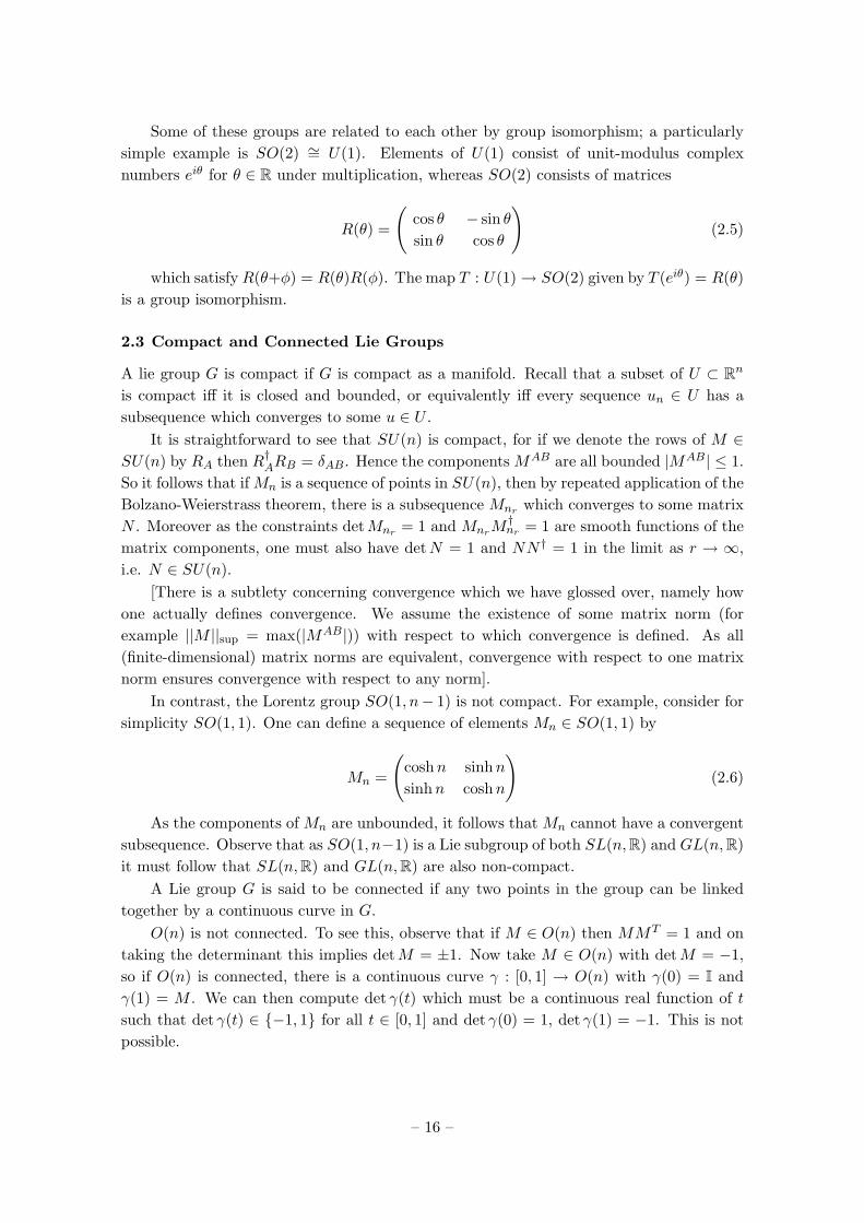
2.3 Compact and Connected Lie Groups

A lie group G is compact if G is compact as a manifold. Recall that a subset of U ⊂ Rn

is compact iff it is closed and bounded, or equivalently iff every sequence un ∈ U has asubsequence which converges to some u ∈ U .

It is straightforward to see that SU(n) is compact, for if we denote the rows of M ∈SU(n) by RA then R†ARB = δAB. Hence the components MAB are all bounded |MAB| ≤ 1.So it follows that if Mn is a sequence of points in SU(n), then by repeated application of theBolzano-Weierstrass theorem, there is a subsequence Mnr which converges to some matrixN . Moreover as the constraints detMnr = 1 and MnrM

†nr = 1 are smooth functions of the

matrix components, one must also have detN = 1 and NN † = 1 in the limit as r → ∞,i.e. N ∈ SU(n).

[There is a subtlety concerning convergence which we have glossed over, namely howone actually defines convergence. We assume the existence of some matrix norm (forexample ||M ||sup = max(|MAB|)) with respect to which convergence is defined. As all(finite-dimensional) matrix norms are equivalent, convergence with respect to one matrixnorm ensures convergence with respect to any norm].

In contrast, the Lorentz group SO(1, n− 1) is not compact. For example, consider forsimplicity SO(1, 1). One can define a sequence of elements Mn ∈ SO(1, 1) by

Mn =

(coshn sinhnsinhn coshn

)(2.6)

As the components of Mn are unbounded, it follows that Mn cannot have a convergentsubsequence. Observe that as SO(1, n−1) is a Lie subgroup of both SL(n,R) and GL(n,R)it must follow that SL(n,R) and GL(n,R) are also non-compact.

A Lie group G is said to be connected if any two points in the group can be linkedtogether by a continuous curve in G.

O(n) is not connected. To see this, observe that if M ∈ O(n) then MMT = 1 and ontaking the determinant this implies detM = ±1. Now take M ∈ O(n) with detM = −1,so if O(n) is connected, there is a continuous curve γ : [0, 1] → O(n) with γ(0) = I andγ(1) = M . We can then compute det γ(t) which must be a continuous real function of tsuch that det γ(t) ∈ −1, 1 for all t ∈ [0, 1] and det γ(0) = 1, det γ(1) = −1. This is notpossible.

– 16 –

We shall say that two points in G are connected if they can be linked with a continuouscurve. This defines an equivalence relation on G, and hence partitions G into equivalenceclasses of connected points; the equivalence class of g ∈ G is called the connected componentof g. The equivalence class of points of O(n) connected to I is SO(n), which is connected.

2.4 Tangent Vectors

Suppose that U is an open subset of a manifold M , and that the curve γ passes throughsome p ∈ U with γ(t0) = p. Then the curve defines a tangent vector at p, denoted by γp,which maps smooth real functions f : U → R to R according to

γp : f →[ ddt

(f γ(t))]t=t0

(2.7)

The components of the tangent vector are

γmp =[ ddt

((x γ)m)]t=t0

= γp(xm) (2.8)

Note that one can write (using the chain rule)

γp(f) =[ ddt

(f γ(t))]t=t0

=[ ddt

(f x−1 x γ(t))]t=t0

=n∑i=1

∂

∂xi(f x−1)|x(p)(

d

dt(x γ)i)t=t0

=n∑i=1

∂

∂xi(f x−1)|x(p)γ

ip (2.9)

Proposition 1. The set of all tangent vectors at p forms a n-dimensional vector space(where n = dim M), denoted by Tp(M).Proof

Suppose that p lies in the chart U with local co-ordinates x. Suppose also that V ,W ∈ Tp(M) are tangent vectors at p corresponding to the curves γ, σ, where withoutloss of generality we can take γ : (a, b) → M , σ : (a, b) → M with a < t0 < b andγ(t0) = σ(t0) = p

Take a, b ∈ R. Consider the curve ρ in Rn defined by

ρ(t) = a(x γ)(t) + b(x σ)(t)− (a+ b− 1)x(p) (2.10)

where scalar multiplication and vector addition are the standard operations in Rn.Note that ρ(t0) = x(p).

Then define the curve ρ on U by ρ = x−1 ρ, so that ρ(t0) = p.If f is a smooth function on U then by (2.9) it follows that

ρp(f) =n∑i=1

∂

∂xi(f x−1)|x(p)(

d

dt(x ρ)i)t=t0

– 17 –

=n∑i=1

∂

∂xi(f x−1)|x(p)(

d

dtρi(t))t=t0

= an∑i=1

∂

∂xi(f x−1)|x(p)(

d

dt(x γ)i)t=t0

+ b

n∑i=1

∂

∂xi(f x−1)|x(p)(

d

dt(x γ)i)t=t0

= aγp(f) + bσp(f) (2.11)

So it follows that aγp + bσp is the tangent vector to ρ at p.In order to compute the dimension of the vector space it suffices to compute a basis.To do this, define n curves ρ(i) for i = 1, . . . , n passing through p by

(x ρ(i))(t)j = (x(p))j + tδji (2.12)

Using (2.9) it is straightforward to compute the tangent vectors to the curves ρ(i) atp;

ρ(i)p(f) =∂

∂xi(f x−1)|x(p) (2.13)

and hence, if γ is a curve passing through p then (2.9) implies that

γp(f) =n∑i=1

ρ(i)p(f)γip (2.14)

and hence it follows that γp =∑n

i=1 γipρ(i)p. Hence the tangent vectors to the curves

ρ(i) at p span Tp(M). Given the expression (2.13), it is conventional to write the tangent vectors to the curves

ρ(i) at p as

ρ(i)p =( ∂∂xi)p

(2.15)

Lemma 1. Suppose that M1, M2 are smooth manifolds of dimension n1, n2 respectively.Let M = M1×M2 be the Cartesian product manifold and suppose p = (p1, p2) ∈M . ThenTp(M) = Tp1(M1)

⊕Tp2(M2).

ProofSuppose Vp ∈ Tp(M). Then V is the tangent vector to a smooth curve γ(t), with

γ(t0) = p. Write γ(t) = (γ1(t), γ2(t)); γi(t) is then a smooth curve in Mi and γi(t0) = pifor i = 1, 2.

Let f be a smooth function f : M → R. Suppose that xa are local co-ordinates on M1

for a = 1, . . . , n1 and ym are local co-ordinates on M2 for m = 1, . . . , n2 corresponding tocharts U1 ⊂M1 and U2 ⊂M2.

Then one has n1 + n2 local co-ordinates zα on M where if q = (q1, q2) ∈ U1 × U2,

z(q1, q2) =(x1(q1), . . . , xn1(q1), y1(q2), . . . , yn2(q2)

)(2.16)

– 18 –

Note that f1(q1) = f(q1, q2) is a smooth function of q1 when q2 is fixed, and f2(q2) =f(q1, q2) is a smooth function of q2 when q1 is fixed.

Then using the chain rule

Vpf =n1+n2∑α=1

∂

∂zα(f z−1)|z(p)

d

dt((z γ)α(t))|t=t0

=n1∑a=1

∂

∂xa(f1 x−1)|(x(p1),y(q2))

d

dt((x γ1)a(t))|t=t0

+n2∑j=1

∂

∂yj(f2 y−1)|(x(p1),y(q2))

d

dt((y γ2)j(t))|t=t0

= (V (1)p + V (2)p)f (2.17)

where V (1)p is the tangent vector to γ1 at p, and V (2)p is the tangent vector to γ2 atp. Hence Vp = V (1)p + V (2)p. Conversely, given two smooth curves γ1(t), γ2(t) in M1, M2

passing through p1 and p2 at t = t0, with associated tangent vectors V (1)p and V (2)p, onecan construct the smooth curve γ(t) = (γ1(t), γ2(t)) in M passing through p = (p1, p2) att = t0. Then (2.17) shows that V (1)p + V (2)p can be written as Vp ∈ Tp(M).

2.5 Vector Fields and Commutators

The tangent space of M , T (M) consists of the union

T (M) =⋃p∈M

Tp(M) (2.18)

A vector field V on M is a map V : M → T (M) such that V (p) = Vp ∈ Tp(M).Note that T (M) is a vector space with addition and scalar multiplication defined by

(X + Y )(f) = X(f) + Y (f) (2.19)

where X,Y ∈ T (M) and f : M → R is smooth, and

(αX)(f) = αX(f) (2.20)

for constant α ∈ R.At a point p ∈ M , one can decompose Vp into its components with respect to a

particular chart as

Vp = V ip

( ∂∂xi)p

(2.21)

It is conventional to write

V = V i(∂

∂xi) (2.22)

where V i = (V x−1)(xi) are functions Rn → R and ( ∂∂xi

) is a locally defined vectorfield which satisfies

– 19 –

(∂

∂xi)xj = δji (2.23)

It follows that T (M) is n-dimensional with a local basis given by the ( ∂∂xi

). The vectorfield is called smooth if the functions V i are smooth functions on Rn.

Suppose now that f is a smooth function on M and that V , W are vector fields on M .Then note that V f can be regarded as a function M → R defined by

(V f)(p) = Vpf (2.24)

Hence one can act on V f with Wp at some p ∈M to find

Wp(V f) = W ip

( ∂∂xi)p(V f)

= W ip

( ∂∂xi)p(V j ∂

∂xj(f x−1))|x(p)

= W ip

∂V j

∂xi|x(p)(

∂

∂xj(f x−1))|x(p)

+ W ipV

jp (

∂2

∂xi∂xj(f x−1))|x(p) (2.25)

The fact that there are second order derivatives acting on f means that we cannotwrite Wp(V f) = Zpf for some vector field Z.

However, these second order derivatives can be removed by taking the difference

Wp(V f)− Vp(Wf) =(W ip

∂V j

∂xi|x(p) − V i

p

∂W j

∂xi|x(p)

)(∂

∂xj(f x−1))|x(p) (2.26)

which can be written as Zpf where Z is a vector field called the commutator or alter-natively the Lie bracket of W and V which we denote by [W,V ] with components

[W,V ]j = W i∂Vj

∂xi− V i∂W

j

∂xi(2.27)

Exercise:Prove that the Lie bracket satisfies

i) Skew-symmetry: [X,Y ] = −[Y,X] for all smooth vector fields X, Y ∈ T (M).

ii) Linearity: [αX+βY, Z] = α[X,Z] +β[Y,Z] for α, β constants and X, Y , Z ∈ T (M).

iii) The Jacobi identity: [[X,Y ], Z]+[[Z,X], Y ]+[[Y, Z], X] = 0 for all X, Y , Z ∈ T (M).

Definition 11. Let V be a smooth vector field on M . An integral curve σ(t) of V is acurve whose tangent vector at σ(t) is V |σ(t), i.e.

d

dt(σi(t)) = V i

σ(t) (2.28)

where in a slight abuse of notation, σi(t) = (x σ)i(t) for some local co-ordinates x.Such a curve is guaranteed to exist and to be unique (at least locally, given an initialcondition), by the standard existence and uniqueness theorems for ODE’s.

– 20 –

2.6 Push-Forwards of Vector Fields

Suppose that M , N are two smooth manifolds and f : M → N is a smooth map. Thenthere is an induced map

f∗ : T (M)→ T (N) (2.29)

which maps the tangent vector of a curve γ passing through a point p ∈ M to thetangent vector of the curve f γ passing through f(p) ∈ N .

In particular, for each smooth function h on N , and if γ is a curve passing throughp ∈M with γ(0) = p, and if Vp ∈ Tp(M) is the tangent vector of γ at p then f∗Vp ∈ Tf(p)(N)is given by

(f∗Vp)h =d

dt

(h (f γ)

)t=0

= Vp(h f) (2.30)

Hence it is clear that the push-forward map f∗ is linear on the space of tangent vectors.Note that if M , N and Q are manifolds, and f : M → N , g : N → Q are smooth

functions then if h : Q→ R is smooth and p ∈M ,

((g f)∗Vp

)(h) = Vp(h (g f))

= Vp((h g) f)= (f∗Vp)(h g)=(g∗(f∗Vp)

)(h) (2.31)

and hence

(g f)∗ = g∗ f∗ (2.32)

2.7 Left-Invariant Vector Fields

Suppose that G is a Lie group and a, g ∈ G. Define the operation of left-translationLa : G→ G by

Lag = ag (2.33)

La defined in this fashion is a differentiable invertible map from G onto G. Hence, onecan construct the push-forward La∗ of vector fields on G with respect to La.

Definition 12. A vector field X ∈ T (G) is said to be left-invariant if

La∗(X|g) = X|ag (2.34)

Given v ∈ Te(G) one can construct a unique left-invariant vector field X(v) ∈ T (G)with the property that X(v)e = v using the push-forward by

– 21 –

X(v)|g = Lg∗v (2.35)

To see that X(v) is left-invariant, note that

X(v)|ag = L(ag)∗v (2.36)

but from (2.32) it follows that as Lag = La Lg we must have

L(ag)∗v = (La Lg)∗v = La∗(Lg∗v) = La∗X(v)g (2.37)

so X(v) is left-invariant. Hence there is a 1-1 correspondence between elements of thetangent space at e and the set of left-invariant vector fields.

Proposition 2. The set of left-invariant vector fields is closed under the Lie bracket, i.e.if X, Y ∈ T (G) are left-invariant then so is [X,Y ].Proof

Suppose that f : G→ R is a smooth function. Then

(La∗[X,Y ]g

)f = [X,Y ]g(f La)

= Xg(Y (f La))− Yg(X(f La)) (2.38)

But as X is left-invariant, La∗Xg = Xag so

Xagf = (La∗Xg)f = Xg(f La) (2.39)

so replacing f with Y f in the above we find

Xg((Y f) La) = Xag(Y f) (2.40)

Moreover, as Y is left-invariant, it is straightforward to show that

(Y (f La)

)g = Yg(f La)

= (La∗Yg)f= Yag(f)= (Y f)(ag)=((Y f) La)g (2.41)

so Y (f La) = (Y f) LaHence

Xg(Y (f La))− Yg(X(f La)) = Xg((Y f) La)− Yg((Xf) La)= Xag(Y f)− Yag(Xf)= [X,Y ]agf (2.42)

So La∗[X,Y ]g = [X,Y ]ag, hence [X,Y ] is left-invariant.

– 22 –

2.8 Lie Algebras

Definition 13. Suppose that G is a Lie group. Then the Lie algebra L(G) associatedwith G is Te(G), the tangent space of G at the origin, together with a Lie bracket [ , ] :L(G)× L(G)→ L(G) which is defined by

[v, w] = [L∗v, L∗w]e (2.43)

for v, w ∈ Te(G), L∗v and L∗w denote the smooth vector fields on G obtained by pushingforward v and w by left-multiplication (i.e. L∗v|g = Lg∗v), and [L∗v, L∗w] is the standardvector field commutator. As the Lie bracket on L(G) is obtained from the commutator ofvector fields, it follows that the Lie bracket is

i) Skew-symmetric: [v, w] = −[w, v] for all v, w ∈ L(G).

ii) Linear: [αv1 + βv2, w] = α[v1, w] + β[v2, w] for α, β constants and v1, v2, w ∈ L(G),

iii) and satisfies the Jacobi identity: [[v, w], z] + [[z, v], w] + [[w, z], v] = 0 for all v, w,z ∈ L(G).

where (ii) follows because the push forward map is linear on the space of vector fields,and (iii) follows because as a consequence of Proposition 2, Lg∗[v, w] = [L∗v, L∗w]g.

More generically, one can also define a Lie algebra to be a vector space g equippedwith a map [ , ] : g× g→ g satisfying (i), (ii), (iii) above.

Definition 14. Suppose that Ti : i = 1, . . . , n is a basis for L(G). Then the Ti are calledgenerators of the Lie algebra. As [Ti, Tj ] ∈ L(G) it follows that there are constants cijk

such that

[Ti, Tj ] = cijkTk (2.44)

The constants cijk are called the structure constants of the Lie algebra.The structure constants are constrained by the antisymmetry of the Lie bracket to be

antisymmetric in the first two indices;

cijk = −cjik (2.45)

Also, the Jacobi identity implies

[[Ti, Tj ], Tk] + [[Tj , Tk], Ti] + [[Tk, Ti], Tj ] = 0 (2.46)

which gives an additional constraint on the structure constants

cij`c`k

m + cjk`c`i

m + cki`c`j

m = 0 (2.47)

– 23 –

2.9 Matrix Lie Algebras

The Lie algebras of matrix Lie groups are of particular interest. Suppose that G is a matrixLie group, and V ∈ T (G) is a smooth vector field. Let f be a smooth function of the matrixcomponents gAB. Then if h ∈ G,

Vhf = V mh

∂f

∂xm

= V mh

∂gAB

∂xm∂f

∂gAB

= V ABh

∂f

∂gAB(2.48)

where

V ABh = V m

h

∂gAB

∂xm(2.49)

defines a tangent matrix associated with the components V mh of V at h. Each vector

field has a corresponding tangent matrix, and it will often be most convenient to deal withthese matrices instead of more abstract vector fields as differential operators.

In particular, if γ(t) is some curve in G with tangent vector V then

V f =d

dt(f γ(t))

=dgAB

dt

∂f

∂gAB(2.50)

hence the tangent vector to the curve corresponds to the matrix dgAB

dt . We will fre-quently denote the identity element of a matrix Lie group by e = I

Examples of matrix Lie algebras are

• a) GL(n,R): the co-ordinates of GL(n,R) are the n2 components of the matrices, soGL(n,R) is n2-dimensional. There is no restriction on tangent matrices to curves inGL(n,R), the space of tangent vectors is Mn×n(R), the set of n× n real matrices.

• b) GL(n,C): the co-ordinates of GL(n,C) are the n2 components of the matrices, soGL(n,C) is 2n2-dimensional when viewed as a real manifold. There is no restrictionon tangent matrices to curves in GL(n,C), the space of tangent vectors is Mn×n(C),the set of n× n complex matrices.

• c) SL(n,R): Suppose that M(t) is a curve in SL(n,R) with M(0) = I. To computethe restrictions on the tangent vectors to the curve note that

detM(t) = 1 (2.51)

so, on differentiating with respect to t,

– 24 –

Tr(M−1(t)

dM(t)dT

)= 0 (2.52)

and so if we denote the tangent vector at the identity to be m = dM(t)dt |t=0 then

Tr m = 0. The tangent vectors correspond to traceless matrices. Hence SL(n,R) isn2 − 1 dimensional.

• d) O(n): suppose that M(t) is a curve in O(n) with M(0) = I. To compute therestrictions on the tangent vectors to the curve note that

M(t)M(t)T = 1 (2.53)

so, on differentiating with respect to t,

dM(t)dt

M(t)T +M(t)dM(t)T

dt= 0 (2.54)

and hence ifm = dM(t)dt |t=0 thenm+mT = 0. The tangents to the curve at the identity

correspond to antisymmetric matrices. There are 12n(n − 1) linearly independent

antisymmetric matrices, hence O(n) is 12n(n− 1)-dimensional.

Note that the Lie algebra of SO(2) is 1-dimensional and is spanned by

T1 =

(0 1

− 1 0

)(2.55)

As [T1, T1] = 0 it follows trivially that the Lie bracket vanishes

• f) SO(n) the group of n × n real matrices such that if M ∈ SO(n) then MMT = 1and detM = 1. By the reasoning in (c) and (e) it follows that the tangent matricesat the identity are skew-symmetric matrices (these are automatically traceless).

As the skew symmetric matrices are automatically traceless, it follows that the Liealgebra L(SO(n)) of SO(n) is identical to the Lie algebra of O(n). If v, w ∈ L(SO(n))are skew-symmetric matrices it is straightforward to show that the matrix commu-tator [v, w] is also skew symmetric, as [v, w]T = (vw − wv)T = wT vT − vTwT =[w, v] = −[v, w]. Hence [v, w] ∈ L(SO(n)) as expected. We will show that vectorfield commutation can be reduced to tangent matrix commutation for matrix Liegroups.

ExerciseShow that the tangent vectors of U(n) at I consist of antihermitian matrices, and the

tangent vectors of SU(n) at I are traceless antihermitian matrices.

– 25 –

Proposition 3. Suppose that G is a matrix Lie group and V is a smooth vector field onG and a ∈ G is fixed. If V denotes the tangent matrix associated with V , then the tangentmatrix associated with the push-forward La∗V is aV .Proof

Suppose h ∈ G, and f : G → R is a smooth function on G. Consider the tangentvector La∗Vh defined at ah

Then

(La∗Vh)f = Vh(f La)= Vhf (2.56)

where f(g) = f(ag).So

(La∗Vh)f = V ABh

∂f

∂gAB|h

= V ABh

∂f

∂gPQ|ah

∂

∂gAB((ag)PQ)

= V ABh

∂f

∂gPB|ahaPA

= (aV )AB∂f

∂gAB|ah (2.57)

So it follows that the tangent matrix associated with La∗Vh is aV . Using this result, it is possible to re-interpret the commutator of two left-invariant

vector fields in terms of the matrix commutators of their associated matrices.

Proposition 4. Suppose that G is a matrix Lie group and that v, w ∈ Te(G) and V , Ware the left-invariant vector fields defined by Vg = Lg∗v, Wg = Lg∗w. Then the matrixassociated with [V,W ]e is the matrix commutator of [v, w] where v and w are the matricesassociated with v and w.Proof

By definition, the matrix associated with [V,W ] is

[V,W ]AB = [V,W ]m∂gAB

∂xm

= V p∂Wm

∂xp∂gAB

∂xm−W p∂V

m

∂xp∂gAB

∂xm

= V p ∂

∂xp(Wm∂g

AB

∂xm)−W p ∂

∂xp(V m∂g

AB

∂xm)

= V p∂WAB

∂xp−W p∂V

AB

∂xp(2.58)

where V and W denote the matrices associated with V and W . But from the previousproposition Vg

AB= gAC vCB and Wg

AB= gACwCB so

– 26 –

[V,W ]ABe = V P ∂gAC

∂xp|ewCB −WP ∂g

AC

∂xp|evCB

= vACwCB − wAC vCB

= [v, w]AB (2.59)

as required. We have therefore shown that if G is a matrix Lie group then the elements L(G) can be

associated with matrices and the Lie bracket is then simply standard matrix commutationby Proposition 4 (which can be directly checked satisfies all three of the Lie bracket forLie algebras). In the literature, it is often conventional to denote the Lie algebra of SO(n)by so(n), su(n) is the Lie algebra of SU(n), u(n) the Lie algebra for U(n) etc. We willhowever continue to use the notation L(G) for the Lie algebra of Lie group G.

Observe that the image [L(G),L(G)] under the Lie bracket need not be the whole ofL(G). This is clear for SO(2), as the Lie bracket vanishes identically in that case. Recallthat the Lie bracket on R viewed as a Lie group under addition vanishes identically aswell. If G is a connected 1-dimensional Lie group then G must either be isomorphic to Ror SO(2) (equivalently U(1)).

2.10 One Parameter Subgroups

Definition 15. A curve σ : R→ G is called a one-parameter subgroup if σ(s)σ(t) = σ(s+t)for all s, t ∈ R.

Note that if σ(t) is a 1-parameter subgroup then σ(0) = e.We shall show that these subgroups arise naturally as integral curves of left-invariant

vector fields.

Proposition 5. Suppose that V is a left-invariant vector field. Let σ(t) be the integralcurve of V which passes through e when t = 0.

Then σ(t) is a 1-parameter subgroup of G.Proof

Let x denote some local co-ordinates.Consider the curves χ1(t) = σ(s)σ(t) and χ2(t) = σ(s+ t) for fixed s.These satisfy the same initial conditions χ1(0) = χ2(0) = σ(s).By definition, χ2 satisfies the ODE

d

dt((x χ2(t))n) =

d

d(s+ t)((x σ(s+ t))n)

= Vσ(s+t)(xn)

= Vχ2(t)(xn) (2.60)

Consider

d

dt((x χ1(t))n) =

d

dt

((x Lσ(s) σ(t))n

)

– 27 –

=d

dt

(((x Lσ(s) x−1) (x σ)(t))n

)=

∂

∂xm((x Lσ(s) x−1)n

)|xσ(t)

d

dt((x σ(t))m) (2.61)

where we have used the chain rule. But by definition of σ(t),

d

dt((x σ(t))m) = V m

σ(t) (2.62)

Hence, substituting this into the above:

d

dt((x χ1(t))n) = V m

σ(t)

∂

∂xm((x Lσ(s) x−1)n

)|xσ(t)

= Vσ(t)((x Lσ(s))n)= (Lσ(s)∗Vσ(t))(x

n) (by definition of push− forward)= Vχ1(t)(x

n) (as V is left− invariant) (2.63)

So χ1, χ2 satisfy the same ODE with the same initial conditions.Hence it follows that σ(s)σ(t) = σ(s+ t), i.e. σ defines a 1-parameter subgroup. The converse is also true: a 1-parameter subgroup σ(t) has left-invariant tangent

vectors

Proposition 6. Suppose σ(t) is a 1-parameter subgroup of G with tangent vector V . Sup-pose Ve = v. Then Vσ(t) = Lσ(t)∗v, i.e. the tangent vectors are obtained by pushing forwardthe tangent vector at the identity.Proof

Suppose f : G→ R is a smooth function. Then

Vσ(t)f =d

dt

((f σ)(t)

)= lim

h→0

(f(σ(t+ h))− f(σ(t))h

)= lim

h→0

(f(σ(t)σ(h))− f(σ(t))h

)=

d

dt′(f Lσ(t) σ(t′))|t′=0

= (Lσ(t)∗v)f (2.64)

so Vσ(t) = Lσ(t)∗v. From this we obtain the corollory

Corollory 1. Suppose that σ(t), µ(t) are two 1-parameter subgroups of G with tangentvectors V , W respectively, with Ve = We = u. Then σ(t) = µ(t) for all t.Proof

Note that

d

dt

((x σ(t))n

)= Vσ(t)x

n

– 28 –

= (Lσ(t)∗u)xn (2.65)

and also

d

dt

((x µ(t))n

)= Wσ(t)x

n

= (Lµ(t)∗u)xn (2.66)

So x σ and x µ satisfy the same ODE and with the same initial conditions, henceσ(t) = µ(t).

2.11 Exponentiation

Definition 16. Suppose v ∈ Te(G), Then we define the exponential map exp : Te(G)→ G

by

exp(v) = σv(1) (2.67)

where σv(t) denotes the 1-parameter subgroup generated by X(v), and X(v) is theleft-invariant vector field obtained via the push-forward X(v)g = Lg∗v

Note that exp(0) = e.

Proposition 7. If v ∈ Te(G) and t ∈ R then

exp(tv) = σv(t) (2.68)

and hence exp((t1 + t2)v) = exp(t1v)exp(t2v).Proof

Take a ∈ R, a 6= 0. Note that σv(at) and σav(t) are both 1-parameter subgroups of G.The tangent vector to σav(t) at the origin is av.

We also compute the tangent vector to σv(at) at e via

d

dt

((x σ(at))n

)t=0

= ad

d(at)((x σ(at))n

)at=0

= avn (2.69)

So σv(at) and σav(t) have the same tangent vector av at the origin. Therefore σv(at) =σav(t).

Hence

exp(tv) = σtv(1) = σv(t) (2.70)

as required.

– 29 –

2.12 Exponentiation on matrix Lie groups

Suppose that G is a matrix Lie group, and v ∈ Te(G) is some tangent matrix. Theexponential exp(tv) produces a curve in G with d

dt(exp(tv))|t=0 = v satisfying exp((t1 +t2)v) = exp(t1v) exp(t2v)

It is then straightforward to show that

d

dt(exp(tv))|t=t0 = lim

t→0

(t−1(exp((t0 + t)v)− exp(t0v))

)= lim

t→0

(t−1(exp(tv)− I) exp(t0v)

)= v exp(t0v) (2.71)

Similarly, one also finds ddt(exp(tv))|t=t0 = exp(t0v)v, so v commutes with exp(tv).

It is clear that ddt exp(tv) = v exp(tv) implies that exp(tv) is infinitely differentiable (as

expected as the integral curve is smooth by construction). Then by elementary analysis,one can compute the power series expansion for exp(tv) as

exp(tv) =∞∑n=0

tnvn

n!(2.72)

with a remainder term which converges to 0 (with respect to the supremum norm onmatrices, for example). Hence, for matrix Lie groups, the Lie group exponential operatorcorresponds to the usual operation of matrix exponentiation.

Comment: Suppose that G1 and G2 are Lie groups. Then G = G1×G2 is a Lie group,and by Lemma 1, L(G) = L(G1)

⊕L(G2).

Conversely, suppose Lie groups G, G1, G2 are such that L(G) = L(G1)⊕L(G2). Then

by exponentiation, it follows that, at least in a local neighbourhood of e, G has the localgeometric structure of G1×G2. However, as it is not in general possible to reconstruct thewhole group in this fashion, one cannot say that G = G1×G2 globally (typically there willbe some periodic identification somewhere in the Cartesian product group).

In general, one cannot reconstruct the entire Lie group by exponentiating elements ofthe Lie algebra. Consider for example, SO(2) and O(2). Both L(O(2)) and L(SO(2)) aregenerated by

T1 =

(0 1

− 1 0

)(2.73)

however it is straightforward to show that

eθT1 =

(cos θ sin θ

− sin θ cos θ

)(2.74)

which always has determinant +1. So SO(2) = exp(L(SO(2))) butO(2) 6= exp(L(O(2))).However, there do exist neighbourhoods B0 of 0 ∈ L(G) and B1 of I ∈ G such that themap exp : B0 → B1 is invertible. (The inverse is called log by convention).

– 30 –

2.13 Integration on Lie Groups

Suppose that G is a matrix Lie group, and let V be a left-invariant vector field on G, andsuppose that the associated tangent matrix to V at the identity is v.

Then if x are some local co-ordinates on G, we know that

g(x)v = V mg(x)

∂g(x)∂xm

(2.75)

From this formula, it is clear that if h ∈ G is a constant matrix then

V mg(x) = V m

hg(x) (2.76)

If H = h1, . . . , hr is a finite group, and f : H → R is a function, then the integral off over H is simply

r∑i=1

f(hi) (2.77)

and note that if h ∈ H is fixed then

r∑i=1

f(hi) =r∑i=1

f(hhi) (2.78)

We wish to construct an analogous integral over a matrix Lie group G. Suppose thatx, y are co-ordinates on G and define

dnx = dx1 . . . dxn, dny = dy1 . . . dyn (2.79)

Note that dnx and dny are related by

dnx = J−1dny (2.80)

where J is the Jacobian J = det( ∂yi∂xj

).

Now suppose that µi for i = 1, . . . , n is a basis of left-invariant vector fields. Then

µi|g(x) = µji,g(x)

∂

∂xj(2.81)

Then we have

µji,g(x)

∂

∂xj= µji,g(x)

∂yk

∂xj∂

∂yk= µji,g(y)

∂

∂yj(2.82)

so

µji,g(y) = µki,g(x)

∂yj

∂xk(2.83)

and hence

det(µji,g(x)

)= J−1 det

(µji,g(y)

)(2.84)

Motivated by this, we make the

– 31 –

Definition 17. The Haar measure is defined by

dnx(

det(µji,g(x)))−1 (2.85)

Then by the previous reasoning,

dnx(

det(µji,g(x)))−1 = dny

(det(µji,g(y))

)−1 (2.86)

so the measure is invariant under changes of co-ordinates.Also, if h is a constant matrix, then as the µi are left-invariant, µji,g(x) = µji,hg(x), and

sodnx

(det(µji,g(x))

)−1 = dnx(

det(µji,hg(x)))−1 (2.87)

It follows that if f : G→ R, then∫dnx

(det(µji,g(x))

)−1f(g(x)) =

∫dnx

(det(µji,g(x))

)−1f(hg(x)) (2.88)

It can be shown that the Haar measure (up to multiplication by a non-zero constant)is the unique measure with this property.

Example: SL(2,R)Consider g ∈ SL(2,R),

g =

(a b

c d

)(2.89)

for a, b, c, d ∈ R constrained by ad− bc = 1. Note that

g−1 =

(d −b−c a

)(2.90)

We take co-ordinates x1 = b, x2 = c, x3 = d (in some neighbourhood of the identity).Then

g−1 ∂g

∂x1=

(c d

− c2

d −c

), g−1 ∂g

∂x2=

(0 01d 0

), g−1 ∂g

∂x3=

(−a −bacd a

)(2.91)

Take

v1 =

(1 00 −1

), v2 =

(0 01 0

), v3 =

(0 10 0

)(2.92)

to be a basis for L(SL(2,R)). Then note that

v1 = −bg−1 ∂g

∂x1+ cg−1 ∂g

∂x2− dg−1 ∂g

∂x3

– 32 –

v2 = dg−1 ∂g

∂x2

v3 = ag−1 ∂g

∂x1+ cg−1 ∂g

∂x3(2.93)

It follows that the left-invariant vector fields obtained from pushing-forward the vectorfields associated with v1, v2, v3 at the identity with L∗ are

µ1 = −b ∂

∂x1+ c

∂

∂x2− d ∂

∂x3

µ2 = d∂

∂x2

µ3 = a∂

∂x1+ c

∂

∂x3(2.94)

So the matrix µji is

(µji ) =

−b c −d0 d 0a 0 c

(2.95)

As det(µji ) = d it follows that the Haar measure in these co-ordinates is 1d db dc dd.

2.14 Representations of Lie Groups

Definition 18. Let V be a finite dimensional vector space (over R or C) and let GL(V )denote the space of invertible linear transformations V → V . Then a representation of aLie group G acting on V is a map D : G→ GL(V ) such that

D(g1g2) = D(g1)D(g2) (2.96)

for all g2, g2 ∈ G. (i.e. D is a homomorphism). The dimension of the representation isgiven by dim D = dim V .

Lemma 2. If D is a representation of G then D(e) = 1 where 1 ∈ GL(V ) is the identitytransformation, and if g ∈ G then D(g−1) = (D(g))−1.Proof

Note that D(e) = D(ee) = D(e)D(e) and so it follows that D(e) = 1 where 1 ∈ GL(V )is the identity transformation.

If g ∈ G then 1 = D(e) = D(gg−1) = D(g)D(g−1), so D(g−1) = (D(g))−1. If M(V ) denotes the set of all linear transformations V → V , and D : G → M(V )

satisfies D(e) = 1 together with the condition (2.96) then it follows from the reasoningused in the Lemma above that D(g) is invertible for all g ∈ G, with inverse D(g−1), andhence D is a representation.

We next define some useful representations

Definition 19. The trivial representation is defined by D(g) = 1 for all g ∈ G

– 33 –

Definition 20. If G is a matrix Lie group which is a subgroup of GL(n,R) or GL(n,C)then the group elements themselves act directly on n-component vectors. The fundamentalrepresentation is then defined by D(g) = g.

Definition 21. If G is a matrix Lie group then the adjoint representation Ad : G →GL(L(G)) is defined by

(Ad(g))X = gXg−1 (2.97)

for g ∈ G and X ∈ L(G) is a tangent matrix.

Lemma 3. Ad(g) as defined above is a representationProof

We first verify that if X ∈ L(g) then Ad(g)X ∈ L(G).Fix g ∈ G. Next, recall that if X ∈ L(G) then there is some smooth curve in G, γ(t)

such that X = dγ(t)dt |t=0. Define a new smooth curve in G by ρ(t) = gγ(t)g−1, then the

tangent matrix to ρ(t) at t = 0 is given by dρ(t)dt |t=0 = g dγ(t)

dt |t=0g−1 = gXg−1.

Hence Ad(g)X ∈ L(G).It is clear that Ad(g) is a linear transformation on X ∈ L(G).Note that Ad(e)X = eXe−1 = X, so Ad(e) = 1. Also, if g1, g2 ∈ G then

Ad(g1g2)X = (g1g2)X(g1g2)−1

= g1g2Xg−12 g−1

1

= g1(g2Xg−12 )g−1

1

= g1(Ad(g2)X)g−11

= Ad(g1)Ad(g2)X (2.98)

hence Ad(g1g2) = Ad(g1)Ad(g2).It then follows that Ad(g)Ad(g−1) = Ad(gg−1) = Ad(e) = 1 so Ad(g) is invertible.

Definition 22. Suppose D is a representation of G acting on V . A subspace W ⊂ V iscalled an invariant subspace if D(g)w ∈W for all g ∈ G and w ∈W .

Definition 23. Suppose D is a representation of G acting on V . Then D is reducible ifthere is an invariant subspace W of V with W 6= 0 and W 6= V . If the only invariantsubspaces of V are 0 and V then D is called irreducible.

Definition 24. A representation D is called totally reducible if there exists a direct sum de-composition of V into subspaces Wi, V = W1

⊕W2⊕...⊕Wk where the Wi are invariant

subspaces with respect to D and D restricted to Wi is irreducible.In terms of matrices, if D is totally reducible, then there is some basis of V in which

D has a block diagonal form

D(g) =

D1(g) 00 D2(g)

. . .

(2.99)

– 34 –

Di(g) denotes D(g) restricted to Wi.

Definition 25. A representation D of G acting on V is faithful if D(g) = 1 only if g = e.

Definition 26. Suppose that D is a representation of G acting on V where V is a vectorspace over C equipped with an inner product. Then D is a unitary representation if D(g) :V → V satisfies D(g)D(g)† = 1 for all g ∈ G.

Proposition 8. A finite dimensional unitary representation is totally reducibleProof

If D is irreducible then we are done. Otherwise, suppose that W is an invariantsubspace. Write V = W ⊕W⊥. Suppose v ∈W⊥. Then if w ∈W and g ∈ g,

〈D(g)v, w〉 = 〈v,D(g)†w〉= 〈v,D(g)−1w〉= 〈v,D(g−1)w〉= 0 (2.100)

as D(g−1)w ∈W because W is an invariant subspace.Hence it follows that if v ∈ W⊥ then D(g)v ∈ W⊥ and so W⊥ is also an invariant

subspace. Repeating this process by considering D restricted to the invariant subspaces Wand W⊥ one obtains a direct sum decomposition of V into invariant (orthogonal) subspacesWi such that D restricted to Wi is irreducible.

Proposition 9. Let V1, V2 be finite dimensional vector spaces. Suppose D is a represen-tation of G acting on V1, and A : V1 → V2 is an invertible linear transformation. DefineD(g) = AD(g)A−1. Then D is a representation of G on V2.Proof

As D is a composition of invertible linear transformations, D is also an invertible lineartransformation on V2.

Also, if g1, g2 ∈ G

D(g1g2) = AD(g1g2)A−1

= AD(g1)D(g2)A−1

= AD(g1)A−1AD(g2)A−1

= D(g1)D(g2) (2.101)

and hence D is also a representation.

Definition 27. Suppose D is a representation of G acting on V1, and A : V1 → V2 is aninvertible linear transformation. Define D(g) = AD(g)A−1. Then D and D are said to beequivalent representations.

– 35 –

Proposition 10. Schur’s First Lemma: Suppose that D1 and D2 are two irreducible rep-resentations of G acting on V1 and V2 respectively and there exists a linear transformationA : V1 → V2 such that

AD1(g) = D2(g)A (2.102)

for all g ∈ G. Then either D1 and D2 are equivalent representations, or A = 0.Proof First note that

Ker A = ψ ∈ V1 : Aψ = 0 (2.103)

is an invariant subspace of D1, because if ψ ∈ Ker A then

AD1(g)ψ = D2(g)Aψ = 0 (2.104)

so D1(g)ψ ∈ Ker A for all g ∈ G. But D1 is irreducible on V1, so one must haveKer A = 0 or Ker A = V1, so A is 1-1 or A = 0.

Similarly,

Im A = φ ∈ V2 : φ = Aψ for some ψ ∈ V1 (2.105)

is an invariant subspace of D2, because if φ ∈ Im A then there is some ψ ∈ V1 suchthat φ = Aψ and hence

D2(g)φ = D2(g)Aψ = AD1(g)ψ (2.106)

and hence D2(g)φ ∈ Im A for all g ∈ G. But D2 is irreducible on V2, so one must haveIm A = 0 or Im A = V2, i.e. A = 0 or A is onto.

Hence either A = 0 or A is both 1-1 and onto i.e. A is invertible. If A is invertiblethen D1 and D2 are equivalent.

Proposition 11. Schur’s Second Lemma: Suppose that D is an irreducible representationof G on V , where V is a vector space over C, and A : V → V is a linear transformationsuch that

AD(g) = D(g)A (2.107)

for all g ∈ G. Then A = λ1 for some λ ∈ C.Proof

As V is over C, A has at least one eigenvalue. Let λ ∈ C be an eigenvalue of A, withcorresponding eigenspace U (U 6= 0). Then U is an invariant subspace of V with respectto D, for if ψ ∈ U then

Aψ = λψ (2.108)

and if g ∈ G, thenAD(g)ψ = D(g)Aψ = D(g)(λψ) = λD(g)ψ (2.109)

so D(g)ψ ∈ U .But D is irreducible on V , so this implies U = V (as U 6= 0).Hence it follows that A = λ1.

– 36 –

Definition 28. Suppose that D1 and D2 are representations of the Lie group G over vectorspaces V1 and V2 respectively. Let V = V1

⊗V2 be the standard tensor product vector space

of V1 and V2 consisting of elements v1 ⊗ v2 (v1 ∈ V1 and v2 ∈ V2) in the vector space dualto the space of bilinear forms on V1 × V2. If v1 ⊗ v2 ∈ V then v1 ⊗ v2 acts linearly onbilinear forms Ω via v1⊗v2Ω = Ω(v1, v2). V is equipped with pointwise addition and scalarmultiplication which satisfy (v1 +w1)⊗ (v2 +w2) = v1 ⊗ v2 + v1 ⊗w2 +w1 ⊗ v2 +w1 ⊗w2

and α(v1 ⊗ v2) = (αv1)⊗ v2 = v1 ⊗ (αv2).Then the tensor product representation D is defined as a linear map on V satisfying

D(g)v1 ⊗ v2 = D1(g)v1 ⊗D2(g)v2 (2.110)

for g ∈ G and v1 ∈ V1 and v2 ∈ V2

Proposition 12. The tensor product representation defined above is a representation.Proof

The map D(g) is linear by construction, also

D(e)v1 ⊗ v2 = D1(e)v1 ⊗D2(e)v2 = v1 ⊗ v2 (2.111)

because D1(e) = 1 and D2(e) = 1. Hence D(e) = 1. And if g1, g2 ∈ G then

D(g1g2)v1 ⊗ v2 = D1(g1g2)v1 ⊗D2(g1g2)v2

= D1(g1)D1(g2)v1 ⊗D2(g1)D2(g2)v2

= D(g1)(D1(g2)v1 ⊗D2(g2)v2)= D(g1)D(g2)v1 ⊗ v2 (2.112)

so D(g1g2) = D(g1)D(g2). Hence, this together with D(e) = 1 implies that D(g) isinvertible. So D(g) is a representation.

Note that if D1 is irreducible on V1 and D2 is irreducible on V2 then D = D1⊗D2 is

not generally irreducible on V = V1⊗V2. Indeed, we shall be particularly interested in

decomposing D into irreducible components in several explicit examples.

2.15 Representations of Lie Algebras

Definition 29. Let V be a finite dimensional vector space (over R or C) and let M(V )denote the space of linear transformations V → V . Suppose that L(G) is the Lie algebra of aLie group G. Then a representation of L(G) acting on V is a linear map d : L(G)→M(V )satisfying

d([X,Y ]) = d(X)d(Y )− d(Y )d(X) (2.113)

for all X,Y ∈ L(G). The dimension of the representation is the dimension of V .

Definition 30. The trivial representation of L(G) on V is given by d(X) = 0 for allX ∈ L(G)

– 37 –

Definition 31. If G is a matrix Lie group and hence L(G) is a matrix Lie algebra, thenthe tangent vectors can be regarded as matrices acting directly on n-component vectors.Then we define the fundamental representation of L(G) on V by d(X) = X

There is a particularly natural representation associated with any Lie algebra.

Definition 32. Let L(G) be a Lie algebra. Then the adjoint representation is a represen-tation of L(G) over the vector space L(G), ad : L(G)→M(L(G)) defined by

(ad v)w = [v, w] (2.114)

for v, w ∈ L(G).It is clear from the above that (ad v)w is linear in w , hence ad v ∈ M(L(G)), and

ad v is also linear in v.Moreover, if v1, v2, w ∈ L(G) then

(ad [v1, v2])w = [[v1, v2], w]= [v1, [v2, w]]− [v2, [v1, w]] (using the Jacobi identity)= (ad v1)[v2, w]− (ad v2)[v1, w]= (ad v1)(ad v2)w − (ad v2)(ad v1)w (2.115)

so ad is indeed a representation.

2.16 The Baker-Campbell-Hausdorff (BCH) Formula

The BCH formula states that the product of two exponentials can be written as an expo-nential:

exp(v) exp(w) = exp(v + w +12

[v, w] +112

[v, [v, w]] +112

[[v, w], w] + ...) (2.116)

where ... indicates terms of higher order in v and w. For simplicity we shall consideronly matrix Lie groups, in which case the Lie algebra elements are square matrices.

To obtain the first few terms in this formula, consider etvetw as a function of t and set

eZ(t) = etvetw (2.117)

At t = 0 we must have eZ(0) = I, which is solved by taking Z(0) = 0 (this solution isunique if we limit ourselves to the neighbourhood of the identity on which exp is invertible).Hence we can write Z(t) as a power series

Z(t) = tP +12t2Q+O(t3) (2.118)

where we determine the matrices P and Q by expanding out (2.117) in powers of t:

I + t(v + w) +12t2(w2 + v2 + 2vw) +O(t3) = I + tP +

12t2(Q+ P 2) +O(t3) (2.119)

from which we find P = v + w and Q = [v, w].

– 38 –

Proposition 13. All higher order terms in the power series expansion of Z(t) in the BCHformula depend only on sums of compositions of commutators on v and w.Proof

Suppose that Z(y) is an arbitrary square matrix. Consider

f1(x, y) =∂

∂y(exZ(y)) (2.120)

and

f2(x, y) =∫ 1

1−xe(x−1+t)Z(y)∂Z(y)

∂ye(1−t)Z(y)dt (2.121)

These both satisfy

∂fi∂x

=∂Z(y)∂y

exZ(y) + Z(y)fi(x, y) (2.122)

and fi(0, y) = 0 for i = 1, 2. Hence f1(x, y) = f2(x, y).Now suppose that Z(t) is the matrix appearing in the BCH formula, i.e.

eZ(t) = etvetw (2.123)

Then consider the identity f1(1, t) = f2(1, t). This implies that

v + etvwe−tv =∫ 1

0eyZ(t)∂Z(t)

∂te−yZ(t)dy (2.124)

Now consider the function

g(t) = etvwe−tv (2.125)

this satisfies g(0) = Y and

dng

dtn= etv(ad v)nwe−tv (2.126)

hence the power series expansion of g(t) is given by

etvwe−tv = w +∞∑n=1

tn

n!(ad v)nw (2.127)

Applying this expression to both sides of (2.124) and performing the y-integral, onefinds

v + w +∞∑n=1

tn

n!(ad v)nw =

dZ

dt+∞∑n=1

1(n+ 1)!

(ad Z(t))ndZ

dt(2.128)

Then by expanding out Z(t) =∑∞

n=1 Zntn (as we know that Z(0) = 0), it follows by

induction using the above equation that the Zn can be written as sums of compositions ofcommutators on v and w.

Exercise: Suppose that [v, w] = 0. Show that evew = ev+w.

– 39 –

Proposition 14. Suppose that D is a representation of the matrix Lie group G acting onV . Then there is a representation d of L(G) also on V defined via

d(v) =d

dt

(D(exp(tv))

)|t=0 (2.129)

for v ∈ L(G).Proof

It is convenient to expand out up to O(t3) by

D(etv) = 1 + td(v) + t2h(v) +O(t3) (2.130)

Note that as D is a representation we must have D(e(t1+t2)v) = D(et1v)D(et2v)Hence

1 + (t1 + t2)d(v) + (t1 + t2)2h(v) +O(t3i ) = (1 + t1d(v) + t21h(v))(1 + t2d(v) + t22h(v)) +O(t3i )(2.131)

and so on equating the t1t2 coefficient we find h(v) = 12d(v)2.

Next consider for v, w ∈ L(G)

D(e−tve−twetvetw) = (1− td(v) +12t2d(v)2)(1− td(w) +

12t2d(w)2)

× (1 + td(v) +12t2d(v)2)(1 + td(w) +

12t2d(w)2) +O(t3)

= 1 + t2(d(v)d(w)− d(w)d(v)) +O(t3) (2.132)

But using the BCH formula

e−tve−twetvetw = e−t(v+w)+ 12t2[v,w]+O(t3)et(v+w)+ 1

2t2[v,w]+O(t3)

= et2[v,w]+O(t3) (2.133)

and so

D(e−tve−twetvetw) = D(et2[v,w]+O(t3)) = 1 + t2d([v, w]) +O(t3) (2.134)

Comparing (2.132) with (2.134) we find that

d([v, w]) = d(v)d(w)− d(w)d(v) (2.135)

as required.To show that d is linear, suppose v, w ∈ L(G) and α, β are constants. Then

D(etαvetβw) = D(etαv)D(etβw)= (1 + tαd(v) +O(t2))(1 + tβd(w) +O(t2))= 1 + t(αd(v) + βd(w)) +O(t2) (2.136)

– 40 –

But by the BCH formula

D(etαvetβw) = D(et(αv+βw)+O(t2)) = 1 + td(αv + βw) +O(t2) (2.137)

Hence, comparing the O(t) terms in (2.136) and (2.137) it follows that d(αv + βw) =αd(v) + βd(w).

Proposition 15. If G is a matrix Lie group, then the representation Ad : G→ GL(L(G))induces the representation ad : L(G)→M(L(G)).Proof

If v, w ∈ L(G) then

Ad (etv)w = etvwe−tv

= (1 + tv +O(t2))w(1− tv +O(t2))= w + t[v, w] +O(t2)= (I + tad v +O(t2))w (2.138)

and hence it follows that

d

dt(Ad(etv))|t=0 = ad v (2.139)

as required. We have seen that a representation D of the matrix Lie group G acting on V gives rise

to a representation d of the Lie algebra L(G) on V . A partial converse is true.

Definition 33. Suppose that G is a matrix Lie group. Let d denote a representation ofL(G) on V . Then a representation D is induced locally on G via

D(g) = ed(v) (2.140)

for those g ∈ G such that g = ev.Here we assume that the representation d(v) is realized as a matrix linear transforma-

tion on V , so that the standard matrix exponentiation ed(v) may be taken. The represen-tation D induced by d is generally not globally well-defined, but it is locally well-definedon the neighbourhood of the identity on which exp is invertible.

Proposition 16. The map D given in (2.140) which is locally induced by the representationd of L(G) on V defines a representation.Proof

Clearly, D(g) defines a linear transformation on V .As I = e0 it follows that D(e) = ed(0) = e0 = 1 where d(0) = 0 follows from the

linearity of d.Also, suppose that g1, g2 have g1 = ev1 , g2 = ev2 . Then by the BCH formula we have

g1g2 = ev1+v2+ 12

[v1,v2]+... (2.141)

– 41 –

where . . . denotes a sum of higher order nested commutators by Proposition 13. Hence

D(g1g2) = ed(v1+v2+ 12

[v1,v2]+... )

= ed(v1)+d(v2)+ 12d([v1,v2])+d(... ) (by the linearity of d)

= ed(v1)+d(v2)+ 12

[d(v1),d(v2)]+... (using (2.113))= ed(v1)ed(v2)

= D(g1)D(g2) (2.142)

So D is at least locally a representation. Note that we have made use of the fact that allhigher order terms in the BCH expansion can be written as sums of commutators, togetherwith the property (2.113) of representations of L(G) in proceeding from the second to thethird line of the above equation.

Proposition 17. Suppose that G is a matrix Lie group. If D is a unitary representationof G on V then the induced representation d of L(G) on V is antihermitian.

Conversely, suppose d is a antihermitian representation of L(G) on V , then the (lo-cally) induced representation D of G on V is unitary.Proof

First suppose that D is a unitary representation.Recall that d satisfies D(etX) = I + td(X) +O(t2) for t ∈ R and X ∈ L(G).As D is unitary it follows that D(etX)D(etX)† = I.Hence (I + td(X) +O(t2))(I + td(X) +O(t2))† = I, so expanding out, the O(t) terms

imply d(X) + d(X)† = 0, i.e. d is antihermitian.Conversely, suppose that d is an antihermitian representation of L(G) on V . Let D

denote the (locally) induced representation of G on V .Suppose that g ∈ G is given by g = eX for X ∈ L(G). Then

D(g) = ed(X) (2.143)

Then

D(g)D(g)† = ed(X)(ed(X))†

= ed(X)ed(X)†

= ed(X)e−d(X)

= 1 (2.144)

Hence D(g) is unitary .There are directly analogous definitions for irreducibility of representations of Lie al-

gebras

Definition 34. Suppose d is a representation of L(G) acting on V . A subspace W ⊂ V iscalled an invariant subspace if d(X)ω ∈W for all X ∈ L(G) and ω ∈W .

Definition 35. Suppose d is a representation of L(G) acting on V . Then d is reducibleif there is an invariant subspace W of V with W 6= 0 and W 6= V . If the only invariantsubspaces of V are 0 and V then d is called irreducible.

– 42 –

Definition 36. A representation d of L(G) is called totally reducible if there exists a directsum decomposition of V into subspaces Wi, V = W1

⊕W2⊕...⊕Wk where the Wi are

invariant subspaces with respect to d and d restricted to Wi is irreducible.

Proposition 18. Suppose that G is a matrix Lie group. If D is a representation of G on Vwith invariant subspace W , then W is an invariant subspace of the induced representationd of L(G) on V

Conversely, suppose d is a representation of L(G) on V with invariant subspace W ;then W is an invariant subspace of the (locally) induced representation D of G on V .Proof

Suppose that D is a representation of G on V with invariant subspace W with respectto D. Let d be the induced representation of L(G) on V . If w ∈W and X ∈ L(G) then

d(X)w =d

dt(D(etX))t=0w =

d

dt(D(etX)w)t=0 (2.145)

As D(etX)w ∈W for all t ∈ R it follows that d(X)w ∈W .Conversely, suppose that d is a representation of L(G) on V , and W is an invariant

subspace of V with respect to d. Let D be the locally defined representation of G inducedby d. Then if g ∈ G is given by g = eX for some X ∈ L(G) then if w ∈W ,

D(g)w = ed(X)w =∞∑n=0

1n!dn(X)w (2.146)

However, as W is an invariant subspace of V with respect to d, it follows that dn(X)w ∈Wfor all n ∈ N. Hence D(g)w ∈W .

Note that in this proof we made implicit use of the closure of W .There is also a natural concept of equivalent representations of Lie algebras.

Definition 37. Suppose d is a representation of L(G) acting on V1, and B : V1 → V2 isan invertible linear transformation. Define d(X) = Bd(X)B−1 for X ∈ L(G). Then d andd are said to be equivalent representations.

Exercise: Show that d defined above is a representation of L(G). Also show that if D1,D2 are equivalent representations of G on vector spaces V1 and V2 then the correspondinginduced representations d1 and d2 on V1 and V2 are equivalent; and conversely, if d1 andd2 are equivalent representations of L(G) on V1 and V2 then the locally defined inducedrepresentations D1 and D2 of G are equivalent.

Note that Schur’s lemmas may be applied to representations of Lie algbras in exactlythe same way as to representations of Lie groups.

Hence we have shown that there is (at least locally) a 1-1 correspondence betweenirreducible representations of the Lie group G and the Lie algebra L(G). This is useful,because it enables us to map the analysis of representations of G to those of L(G), andthus the problem reduces to one of linear algebra.

Proposition 19. Suppose that d1 and d2 are representations of L(G) acting on V1 andV2 and let V = V1

⊗V2. Define d = d1 ⊗ 1 + 1 ⊗ d2 as a linear map on V . Then d is a

representation of L(G) acting on V .

– 43 –

ProofIf w1, w2 ∈ L(V ) and α, β are scalars and v1 ⊗ v2 ∈ V then

d(αw1 + βw2)v1 ⊗ v2 = d1(αw1 + βw2)v1 ⊗ v2 + v1 ⊗ d2(αw1 + βw2)v2

= (αd1(w1) + βd1(w2))v1 ⊗ v2 + v1 ⊗ (αd2(w1) + βd2(w2))v2

= αd1(w1)v1 ⊗ v2 + βd1(w2)v1 ⊗ v2

+ αv1 ⊗ d2(w1)v2 + βv1 ⊗ d2(w2)v2

= α(d1(w1)v1 ⊗ v2 + v1 ⊗ d2(w1)v2)+ β(βd1(w2)v1 ⊗ v2 + v1 ⊗ d2(w2)v2)= αd(w1)v1 ⊗ v2 + βd(w2)v2 ⊗ v2 (2.147)

so d is linear on L(G). Also

d([w1, w2])v1 ⊗ v2 = d1([w1, w2])v1 ⊗ v2 + v1d2([w1, w2])v2

= (d1(w1)d1(w2)− d1(w2)d1(w1))v1 ⊗ v2

+ v1 ⊗ (d2(w1)d2(w2)− d2(w2)d2(w1))v2

= d1(w1)d1(w2)v1 ⊗ v2 − d1(w2)d1(w1)v1 ⊗ v2

+ v1 ⊗ d2(w1)d2(w2)v2 − v1 ⊗ d2(w2)d2(w1)v2 (2.148)

Also note that

d(w1)d(w2)v1 ⊗ v2 = d(w1)(d1(w2)v1 ⊗ v2 + v2 ⊗ d2(w2)v2

)= d1(w1)d1(w2)v1 ⊗ v2 + d1(w2)v1 ⊗ d2(w1)v2

+ d1(w1)v1 ⊗ d2(w2)v2 + v1 ⊗ d2(w1)d2(w2)v2 (2.149)

where the sum of the second and third terms in this expression is symmetric in w1 and w2.Hence

d(w1)d(w2)v1 ⊗ v2 − d(w2)d(w1)v1 ⊗ v2 = d1(w1)d1(w2)v1 ⊗ v2 − d1(w2)d1(w1)v1 ⊗ v2

+ v1 ⊗ d2(w1)d2(w2)v2 − v1 ⊗ d2(w2)d2(w1)v2

= d([w1, w2])v1 ⊗ v2 (2.150)

as required .

Proposition 20. Suppose that D1 and D2 are representations of matrix Lie group G onV1 and V2 with induced representations of L(G) on V1 and V2 denoted by d1 and d2. LetD = D1

⊗D2 denote the representation of G on the tensor product V1

⊗V2. Then the

corresponding induced representation of L(G) on V1⊗V2 is d = d1 ⊗ 1 + 1⊗ d2.

Proof Suppose w ∈ L(G), then expanding out in powers of t;

D(etw)v1 ⊗ v2 = D1(etw)v1 ⊗D2(etw)v2

– 44 –

= (v1 + td1(w)v1 +O(t2))⊗ (v2 + td2(w)v2 +O(t2))= v1 ⊗ v2 + t

(d1(w)v1 ⊗ v2 + v1 ⊗ d2(w)v2

)+O(t2)

= v1 ⊗ v2 + t(d1 ⊗ 1 + 1⊗ d2)v1 ⊗ v2 +O(t2) (2.151)

and hence from the O(t) term we find the induced representation d = d1 ⊗ 1 + 1⊗ d2

as required .

2.17 The Killing Form and the Casimir Operator

Definition 38. Suppose that G is a matrix Lie group with Lie algebra L(G). Then forX ∈ L(G), ad X can be realized as a matrix linear transformation on L(G). The Killingform κ is defined by

κ(X,Y ) = Tr (ad Xad Y ) (2.152)

Suppose that Ta is a basis for L(G). Then from the Killing form one obtains a sym-metric matrix

κab = κ(Ta, Tb) (2.153)

Denote the matrix elements of ad Ta by (ad Ta)bc; then note that

(ad Ta)Tb = [Ta, Tb] = cabcTc

= (ad Ta)bcTc (2.154)

Hence (ad Ta)bc = cabc. So it follows that

κab = cadecbe

d (2.155)

Lemma 4. The Killing form is associative: κ(X, [Y,Z]) = κ([X,Y ], Z)Proof

κ(X, [Y,Z]) = Tr (ad Xad [Y,Z])= Tr (ad X(ad Y ad Z − ad Zad Y ))= Tr (ad Xad Y ad Z)− Tr (ad Xad Zad Y )= Tr (ad Xad Y ad Z)− Tr (ad Y ad Xad Z)= Tr ((ad Xad Y − ad Y ad X)ad Z)= Tr (ad [X,Y ]ad Z)= κ([X,Y ], Z) (2.156)

as required. .As κab is symmetric, one can always choose an adapted basis for L(G) in which κab is

a diagonal matrix, and by rescaling the Lie algebra generators, the diagonal entries can beset to +1, 0 or −1.

Definition 39. The Killing form is non-degenerate if κab has no zero diagonal entries inthe adapted basis. The Lie algebra L(G) is then called semi-simple. If all the diagonalentries are −1 then L(G) is said to be a compact Lie algebra.

– 45 –

Lemma 5. Suppose that L(G) is semi-simple. Define cabc = cabdκdc (i.e. lower the last

index of the structure constants with the Killing form). Then cabc is totally antisymmetricin a, b, c.Proof

Note that

κ(Ta, [Tb, Tc]) = cbcdκ(Ta, Td) = cbc

dκad = cbca (2.157)

and

κ([Ta, Tb], Tc) = cabdκ(Td, Tc) = cab

dκdc = cabc = −cbac (2.158)

But by associativity of κ, (2.157) and (2.158) are equal. Hence cbca = −cbac. As cabc isskew symmetric in both the first two and the last two indices, it follows that cabc is totallyantisymmetric.

Definition 40. Suppose that L(G) is a Lie algebra with non-degenerate Killing form, andd is a representation of L(G) on V . The Casimir operator C of L(G) is defined by

C = −∑a,b

(κ−1)abd(Ta)d(Tb) (2.159)

where κ−1 denotes the inverse of the Killing form.

Proposition 21. The Casimir operator commutes with d(X) for all X ∈ L(G)Proof

It suffices to show that [C, d(Ta)] = 0 for all Ta.Note that

[d(Ta), C] = −∑b,c

(κ−1)bc([d(Ta), d(Tb)d(Tc)]

)= −

∑b,c

(κ−1)bc([d(Ta), d(Tb)]d(Tc) + d(Tb)[d(Ta), d(Tc)]

)= −

∑b,c

(κ−1)bc(d[Ta, Tb]d(Tc) + d(Tb)d[Ta, Tc]

)= −

∑b,c

(κ−1)bc(cab

`d(T`)d(Tc) + cac`d(Tb)d(T`)

)= −cac`d(T`)d(Tc)− cac`d(Tc)d(T`)= 0 (2.160)

where we have definedcabc =

∑`

(κ−1)b`ca`c (2.161)

and we note that cabc is antisymmetric in b, c. Note that if d is irreducible then by Schur’s second lemma, C must be a scalar multiple

of the identity.

– 46 –

If L(G) is compact, then working in the adapted basis, C takes a particularly simpleform

C =∑a

d(Ta)d(Ta) (2.162)

– 47 –

3. SU(2) and Isospin

3.1 Lie Algebras of SO(3) and SU(2)

We have shown that the Lie algebra of SO(3) consists of the 3 × 3 antisymmetric realmatrices.

A basis for L(SO(3)) is given by

T1 =

0 0 00 0 −10 1 0

T2 =

0 0 10 0 0−1 0 0

T3 =

0 −1 01 0 00 0 0

(3.1)

Exercise: Show that[Ta, Tb] = εabcTc (3.2)

where εabc is totally antisymmetric and ε123 = 1.Next consider SU(n). Let M(t) be a smooth curve in SU(n) with M(0) = I . Then

M(t) must satisfy

detM(t) = 1 M(t)M(t)† = I (3.3)

Differentiating these constraints we obtain

Tr(M(t)−1dM(t)

dt

)= 0

dM(t)dt

M(t)† +M(t)dM(t)†

dt= 0 (3.4)

Setting t = 0 we findTr m = 0 m+m† = 0 (3.5)

where m = dM(t)dt |t=0. Hence L(SU(n)) consists of the traceless antihermitian matrices.

Exercise: Verify that if X and Y are traceless antihermitian square matrices then so is[X,Y ].

It is convenient to make use of the Pauli matrices σa defined by

σ1 =

(0 11 0

)σ2 =

(0 −ii 0

)σ3 =

(1 00 −1

)(3.6)

which satisfy σaσb = δabI + iεabcσc.Then a basis of traceless antihermitian 2× 2 matrices is given by taking Ta = − i

2σa.It follows that

[Ta, Tb] = εabcTc (3.7)

Comparing (3.2) and (3.7) it is clear that SO(3) and SU(2) have the same Lie algebra.We might therefore expect SO(3) and SU(2) to be similar, at least near to the identity.We shall see that this is true.

Exercise: Using this basis, show that the Lie algebra L(SU(2)) is of compact type.

– 48 –

3.2 Relationship between SO(3) and SU(2)

Proposition 22. The manifold SU(2) can be identified with S3.Proof

Consider

U =

(α µ

β ν

)∈ SU(2) (3.8)

for α, β, µ, ν ∈ C.

Then UU † = I implies that

(α

β

)be orthogonal to

(µ

ν

)with respect to the standard

inner product on C2. As the orthogonal complement to

(α

β

)in C2 is a 1-dimensional

complex vector space spanned by

(−βα

)it follows that µ = −σβ, ν = σα for σ ∈ C.

We also require that

(α

β

)and

(µ

ν

)have unit norm, which fixes

|σ|2 = |α|2 + |β|2 = 1 (3.9)

Finally, the constraint detU = 1 fixes σ = 1.Hence we have shown that

U =

(α −ββ α

)(3.10)

where αα+ ββ = 1. Such U is automatically an element of SU(2). Hence this is the formof the most generic element of SU(2).

Set α = y0 + iy3, β = −y2 + iy1 for y0, y1, y2, y3 ∈ R. Then it is straightforward to seethat

U = y0I + iynσn (3.11)

and αα+ ββ = 1 is equivalent to y20 + y2

1 + y22 + y2

3 = 1, i.e. y ∈ S3.This establishes a smooth invertible map between SU(2) and S3. Note that this map provides an explicit way of seeing that SU(2) is connected, because

S3 is connected.

Proposition 23. There is a 2− 1 correspondence R : SU(2)→ SO(3) between SU(2) andSO(3). The map R is a group homomorphism.Proof Suppose U ∈ SU(2). Define a 3× 3 matrix R(U) via

R(U)mn =12

Tr(σmUσnU

†) (3.12)

By writing U = y0I+iymσm for y0, ym ∈ R satisfying y20 +ypyp = 1, it is straightforward

to show that

Rmn = (y20 − ypyp)δmn + 2εmnqy0yq + 2ymyn (3.13)

– 49 –

(here we have written Rmn = R(U)mn).It is clear that if yp = 0 for p = 1, 2, 3 so that U = ±I, then R = I, so R ∈ SO(3).More generally, suppose that ypyp 6= 0. Then one can set y0 = cosα, yp = sinαzp for

0 < α < 2π and α 6= π. Then the constraint y20 + ypyp = 1 implies that zpzp = 1, i.e z is a

unit vector in R3. The expression (3.13) can be rewritten as

Rmn = cos 2αδmn + sin 2αεmnqzq + (1− cos 2α)zmzn (3.14)

It is then apparent that

Rmnzn = zm (3.15)

and if x is orthogonal to z then

Rmnxn = cos 2αxm + sin 2αεmnqxnzq (3.16)

The transformation R therefore corresponds to a rotation of angle 2α in the plane withunit normal vector z.

It is clear that any non-trivial rotation in SO(3) can be written in this fashion. How-ever, the correspondence is not 1 − 1. To see this explicitly, suppose that two rotationscorresponding to y ∈ S3 and u ∈ S3 are equal. Then

(y20 − ypyp)δmn + 2εmnqy0yq + 2ymyn = (u2

0 − upup)δmn + 2εmnqu0uq + 2umun (3.17)

where y20 + ypyp = u2

0 + upup = 1.From the antisymmetric portion of this matrix we find y0yp = u0up.From the diagonal elements with n = m, we see that

y20 − ypyp + 2(ym)2 = u2

0 − upup + 2(um)2 (3.18)

where p is summed over but m is fixed. Summing over m we find

3y20 − ypyp = 3u2

0 − upup (3.19)

where p is summed over; which together with y20 + ypyp = u2

0 + upup = 1 implies thaty2

0 = u20 and ypyp = upup (sum over p). Substituting back into (3.18) we find y2

m = u2m for

each m = 1, 2, 3.Suppose first that y0 6= 0, then u0 6= 0, and it follows that y0 = ±u0 and yp = ±up for

each p = 1, 2, 3 (with the same sign throughout).Next, suppose y0 = 0. Then u0 = 0 also, and ymyn = umun for each m,n = 1, 2, 3.

Contracting with yn we get (ynyn)ym = (ynun)um for m = 1, 2, 3. As ynyn = 1, this impliesthat ym = λum for m = 1, 2, 3 where λ is constant. Hence, (1− λ2)umun = 0. Contractingover m and n then gives 1 − λ2 = 0, so λ = ±1. Therefore yp = ±up for p = 1, 2, 3 (withthe same sign throughout).

– 50 –

Hence, we have shown that each R ∈ SO(3) corresponds to two elements U and−U ∈ SU(2). These two elements correspond to antipodal points±y ∈ S3. This establishesthe correspondence.

It remains to check that R(U1U2) = R(U1)R(U2) for U1, U2 ∈ SU(2). Note that onwriting

U1 = y0I2 + iynσn, U2 = w0 + iwnσn (3.20)

for y0, yp, w0, wp ∈ R satisfying y20 + ypyp = w2

0 + wpwp = 1 then

U1U2 = u0I2 + iunσn (3.21)

where u0 = y0w0− ypwp and um = y0wm +w0ym− εmpqypwq satisfy u20 +upup = 1. It then

suffices to evaluate directly

R(U1U2)mn = (u20 − upup)δmn + 2εmnqu0uq + 2umun (3.22)

and compare this with

R(U1)mpR(U2)pn =[(y2

0−y`y`)δmp+2εmpqy0yq+2ymyp][

(w20−wrwr)δpn+2εpnrw0wr+2wpwn

](3.23)

On expanding out these two expressions in terms of y and w it becomes an exercise inalgebra to show that R(U1U2)mn = R(U1)mpR(U2)pn as required.

Exercise: Verify the identity R(U1U2)mn = R(U1)mpR(U2)pn.It is conventional to write SU(2) = S3 and SO(3) = S3/Z2, where S3/Z2 is the 3-

sphere with antipodal points identified. SU(2) is called the double cover of SO(3); andthere is an isomorphism SO(3) ∼= SU(2)/Z2.

It can be shown (using topological methods outside the scope of this course) thatSU(2) and SO(3) are not homeomorphic. This is because SU(2) and SO(3) have differentfundamental groups π1. In particular, as SU(2) ∼= S3, and S3 is simply connected, itfollows that π1(SU(2)) is trivial. However, it can be shown that π1(SO(3)) = Z2.

3.3 Irreducible Representations of SU(2)

The standard basis of L(SU(2)) which we have been using is Ta = − i2σa. Suppose that

d is a finite-dimensional irreducible representation of L(SU(2)) on V , where V is a vectorspace over C.

Define

J3 = id(T3), J± =i√2

(d(T1)± id(T2)) (3.24)

Then

[J3, J±] = ±J±, [J+, J−] = J3 (3.25)

As V is a complex vector space, there exists an eigenstate |φ〉 of J3 with some eigenvalueλ, and using (3.25) it follows that

– 51 –

J3J± |φ〉 = (λ± 1)J± |φ〉 (3.26)

and so by simple induction

J3(J±)n |φ〉 = (λ± n)(J±)n |φ〉 (3.27)

for non-negative integer n; i.e. J± are the standard raising and lowering operators.The eigenvalues of J3 are called weights. We have therefore shown that (J±)n |φ〉 eithervanishes or is a J3 eigenstate with eigenvalue λ± n.

Consider the states (J+)n |φ〉. If non-vanishing, these states are linearly independent(as they have different J3 eigenvalues). Hence, as V is finite dimensional, there exists a J3

eigenstate (J+)n |φ〉 which we will refer to as |j, j〉 with eigenvalue j such that J+ |j, j〉 = 0.

Definition 41. j is called the highest weight of the representation. In the context of particlephysics, it is called the spin.

Note that by acting on |j, j〉 with J− other distinct eigenstates of J3 are obtained. Aswe are interested in finite dimensional representations, it follows that (J−)N |j, j〉 = 0 forsome positive integer N (otherwise one could just keep going and the representation wouldbe infinite dimensional). Let k+ 1 be the smallest positive integer for which this happens,and set |ψk〉 = (J−)k |j, j〉, so, by construction, J− |ψk〉 = 0.

Define for ` = 0, . . . , k

|ψ`〉 = (J−)` |j, j〉 (3.28)

Then |ψ`〉 are (non-vanishing) j − ` eigenvectors of J3.Note that

J+ |ψ`〉 = J+(J−)` |j, j〉= (J+J−)(J−)`−1 |j, j〉=([J+, J−] + J−J+

)(J−)`−1 |j, j〉

=(J3 + J−J+

)(J−)`−1 |j, j〉

= (j − (`− 1))(J−)`−1 |j, j〉+ J−J+(J−)`−1 |j, j〉 (3.29)

Repeating this process, one finds by induction

J+ |ψ`〉 =(j − (`− 1) + j − (`− 2) + · · ·+ j − 1 + j

)|ψ`−1〉

= `(j − 12

(`− 1)) |ψ`−1〉 (3.30)

In order to constrain j recall that J− |ψk〉 = 0, so

0 = J+J− |ψk〉=([J+, J−] + J−J+

)|ψk〉

– 52 –

=(J3 + J−J+

)|ψk〉

= (j − k) |ψk〉+ J−(k(j − 1

2(k − 1))

)|ψk−1〉

=(j − k + k(j − 1

2(k − 1))

)|ψk〉

=12

(k + 1)(2j − k) |ψk〉 (3.31)

As k is non-negative, it follows that k = 2jUsing this it is straightforward to prove the following

Proposition 24. V = spanJk− |j, j〉 , Jk−1− |j, j〉 , . . . , |j, j〉 and the highest weight state is

unique.Proof

Consider the vector space V ′ spanned by |ψi〉 for i = 0, . . . , k. This is an invariantsubspace of V with respect to the representation d. As the representation is irreducible onV it follows that V = V ′. In particular, J3 is diagonalizable on V and each eigenspace is1-dimensional.

To prove uniqueness suppose that |φ〉 ∈ V satsfies J+ |φ〉 = 0. As |φ〉 ∈ V it followsthat we can write

|φ〉 =2j∑i=0

ai(J−)i |j, j〉 (3.32)

for constants ai. Applying (J+)2j to both sides of this equation implies a2j = 0. Then,applying (J+)2j−1 implies a2j−1 = 0. Continuing in this way, we obtain a1 = a2 = · · · =a2j−1 = a2j = 0, and so |φ〉 = a0 |j, j〉. So the highest weight state in an irreduciblerepresentation of L(SU(2)) is unique (up to scaling). .

Hence, we have shown that j is half (non-negative) integer, and the representation is2j + 1-dimensional. The irreducible representations are therefore completely characterizedby the value of the weight j.

It is possible to go further, and prove the following theorem (the proof given is thatpresented in [Samelson]):

Theorem 1. **NON-EXAMINABLE** Suppose that d is a representation of L(SU(2))on a complex vector space V . Then V can be decomposed as V = V1 ⊕ · · · ⊕ Vp where Viare invariant subspaces of V such that d restricted to Vi is irreducible.Proof Given in Appendix A.

Note that we have not as yet assumed that the representation originates from a unitaryrepresentation of the Lie group. However, in order to compute normalized states, it willbe convenient to assume this; so in particular, the d(Ta) are antihermitian and hence

J†3 = J3, J†± = J∓ (3.33)

We will assume that the highest weight state |j, j〉 is normalized to 1.Exercise:

– 53 –

Show using (3.30) that 〈ψ`|ψ`〉 = `2(2j − `+ 1) 〈ψ`−1|ψ`−1〉, and hence that

N` ≡ 〈ψ`|ψ`〉 =(2j)!`!

2`(2j − `)!(3.34)

It is conventional to define normalized states |j,m〉 for m = −j, . . . , j via

|j,m〉 =1√Nj−m

|ψj−m〉 (3.35)

the first label denotes the highest weight value j, the m label denotes the eigenstateof J3, J3 |j,m〉 = m |j,m〉. These satisfy (check!)

J− |j,m〉 =1√2

√(j +m)(j −m+ 1) |j,m− 1〉

J+ |j,m− 1〉 =1√2

√(j +m)(j −m+ 1) |j,m〉 (3.36)

Exercise: Show that the Casimir operator C is given by C = −12(J+J−+J−J+ +(J3)2)

and satisfies

C |j,m〉 = −12j(j + 1) |j,m〉 (3.37)

3.3.1 Examples of Low Dimensional Irreducible Representations

It is useful to consider several low-dimensional representations.

i) j = 12 . A normalized basis is given by |12 ,

12〉 and |12 ,−

12〉, with

J+ |12,12〉 = 0

J+ |12,−1

2〉 =

1√2|12,12〉 (3.38)

and

J− |12,12〉 =

1√2|12,−1

2〉

J− |12,−1

2〉 = 0 (3.39)

ii) j = 1. A normalized basis of states is |1, 1〉, |1, 0〉 and |1,−1〉 with

J+ |1, 1〉 = 0J+ |1, 0〉 = |1, 1〉

J+ |1,−1〉 = |1, 0〉 (3.40)

– 54 –

and

J− |1, 1〉 = |1, 0〉J− |1, 0〉 = |1,−1〉

J− |1,−1〉 = 0 (3.41)

iii) j = 32 . A normalized basis of states is |32 ,

32〉, |

32 ,

12〉, |

32 ,−

12〉 and |32 ,−

32〉. with

J+ |32,32〉 = 0

J+ |32,12〉 =

√32|32,32〉

J+ |32,−1

2〉 =√

2 |32,12〉

J+ |32,−3

2〉 =

√32|32,−1

2〉 (3.42)

and

J− |32,32〉 =

√32|32,12〉

J− |32,12〉 =√

2 |32,−1

2〉

J− |32,−1

2〉 =

√32|32,−3

2〉

J− |32,−3

2〉 = 0 (3.43)

3.4 Tensor Product Representations

Suppose that d1 and d2 are two irreducible representations of L(SU(2)) over vector spacesV (1), V (2). Let V = V (1)

⊗V (2) be the tensor product, and d = d1 ⊗ 1 + 1⊗ d2 be the

representation on V .We wish to decompose V into irreducible representations of d (i.e. invariant subspaces

of V on which the restriction of d is irreducible).Denote the states of V (1) by |j1,m〉 for m = −j1, . . . , j1 and those of V (2) by |j2, n〉

for n = −j2, . . . , j2, where j1 and j2 are the highest weights of V (1) and V (2) respectively.Note that |j1,m〉 ⊗ |j2, n〉 for m = −j1, . . . , j1 and n = −j2, . . . , j2 provides a basis for V .

SetJ3(1) = id1(T3), J±(1) =

i√2

(d1(T1)± id1(T2)) (3.44)

andJ3(2) = id2(T3), J±(2) =

i√2

(d2(T1)± id2(T2)) (3.45)

– 55 –

withJ3 = J3(1)⊗ 1 + 1⊗ J3(2), J± = J±(1)⊗ 1 + 1⊗ J±(2) (3.46)

Exercise: Check that J± and J3 satisfy J†3 = J3, J†± = J∓ and

[J3, J±] = ±J±, [J+, J−] = J3 (3.47)

In order to construct the decomposition of V into irreducible representations, first notethat if |ψ(1)〉 ∈ V (1) is a state of weight m1 with respect to J3(1), and |ψ(2)〉 ∈ V (2) isa state of weight m2 with respect to J3(2) then |ψ(1)〉 ⊗ |ψ(2)〉 ∈ V is a state of weightm1 +m2 with respect to J3, i.e. weights add in the tensor product representation.

Using this, it is possible to compute the degeneracy of certain weight states in thetensor product representation. In particular, the maximum possible weight must be j1 + j2which corresponds to |j1, j1〉 ⊗ |j1, j2〉.

Consider the weight j1 + j2 − k for k > 0. In general, j1 + j2 − k can be written as asum of two integers m1 +m2, for m1 ∈ −j1, ..., j1 and m2 ∈ −j2, ..., j2 in k + 1 ways:

j1 + j2 − k = (j1 − k) + j2= (j1 − k + 1) + (j2 − 1). . .

= (j1 − 1) + (j2 − k + 1)= j1 + (j2 − k) (3.48)

provided that j1 − k ≥ −j1 and j2 − k ≥ −j2, or equivalently

k ≤ 2min(j1, j2) = j1 + j2 − |j1 − j2| (3.49)

Consider the state of weight j1 + j2. There is only one such state, and there is no stateof higher weight. Hence it must be a highest weight state of a subspace of V on whichthe tensor product representation is irreducible. This irreducible subspace has dimension2(j1 + j2) + 1, and is denoted by Vj1+j2 Write V = V ′ ⊕ Vj1+j2 .

Next consider the states in V ′. The highest possible weight is j1 + j2 − 1. In V therewere two linearly independent states of this weight, however one of these lies in Vj1+j2 , anddoes not lie in V ′. The remaining state of weight j1 + j2 − 1 is of highest weight in V ′ andhence must be a highest weight state of a subspace (of dimension 2(j1 + j2)− 1) of V ′, onwhich the tensor product representation is irreducible. Denote this subspace by Vj1+j2−1.Note that by construction Vj1+j2 ∩ Vj1+j2−1 = 0.

One can continue inductively in this fashion: for each j = |j1−j2|, |j1−j2|+1, . . . j1+j2there is a subspace Vj (of dimension 2j+1) on which the tensor product representation is ir-reducible, with highest weight j, and Vj∩Vk = 0 if j 6= k. In fact these subspaces accountfor all of the elements in V . To see this, compute the dimension of V|j1−j2|

⊕· · ·⊕Vj1+j2 :

We find

dim V|j1−j2|⊕· · ·⊕

Vj1+j2 =j1+j2∑

j=|j1−j2|

(2j + 1)

– 56 –

=j1+j2−|j1−j2|∑

n=0

(2(|j1 − j2|+ n) + 1)

= (1 + 2j1)(1 + 2j2)= dim V (3.50)

Hence we have decomposed V = V|j1−j2|⊕· · ·⊕Vj1+j2 into irreducible subspaces Vj

where Vj has highest weight j and is of dimension 2j + 1.

3.4.1 Examples of Tensor Product Decompositions

We shall consider two simple spin combinations which are of physical interest.Firstly, take the spin 1/2 ⊗ spin 1/2 composite system. As j1 = j2 = 1

2 there are twopossible values for the composite spin, j = 1 or j = 0, and the tensor product space is4-dimensional.

For the j = 1 states, the highest weight state can be written as

|1, 1〉 = |12,12〉 ⊗ |1

2,12〉 (3.51)

Applying J− to both sides we find

|1, 0〉 =1√2

(|12,−1

2〉 ⊗ |1

2,12〉+ |1

2,12〉 ⊗ |1

2,−1

2〉)

(3.52)

and applying J− once more

|1,−1〉 = |12,−1

2〉 ⊗ |1

2,−1

2〉 (3.53)

The remaining possible spin is j = 0. This has only one state, which must have theform

|0, 0〉 = c0 |12,12〉 ⊗ |1

2,−1

2〉+ c1 |

12,−1

2〉 ⊗ |1

2,12〉 (3.54)

for constants c0, c1 to be fixed. Applying J+ to both sides we get

(c0 + c1) |12,12〉 ⊗ |1

2,12〉 = 0 (3.55)

so c1 = −c0. Then on making the appropriate normalization we find

|0, 0〉 =1√2

(|12,−1

2〉 ⊗ |1

2,12〉 − |1

2,12〉 ⊗ |1

2,−1

2〉)

(3.56)

Next, take the spin 1 ⊗ spin 1/2 composite system. As j1 = 1, j2 = 12 there are two

possible values for the composite spin, j = 12 or j = 3

2 , and the tensor product space is6-dimensional.

For the j = 32 states, the state with greatest weight is

|32,32〉 = |1, 1〉 ⊗ |1

2,12〉 (3.57)

– 57 –

Applying J− to both sides gives

|32,12〉 =

√23|1, 0〉 ⊗ |1

2,12〉+

1√3|1, 1〉 ⊗ |1

2,−1

2〉 (3.58)

Further applications of J− give

|32,−1

2〉 =

1√3|1,−1〉 ⊗ |1

2,12〉+

√23|1, 0〉 ⊗ |1

2,−1

2〉 (3.59)

and|32,−3

2〉 = |1,−1〉 ⊗ |1

2,−1

2〉 (3.60)

For the j = 12 states, the state with maximal weight can be written as a linear combi-

nation|12,12〉 = c0 |1, 1〉 ⊗ |

12,−1

2〉+ c1 |1, 0〉 ⊗ |

12,12〉 (3.61)

for some constants c0, c1 to be determined. Then

0 = J+ |12,12〉 = (c1 +

1√2c0) |1, 1〉 ⊗ |1

2,12〉 (3.62)

so c1 = − 1√2c0. On making a unit normalization, we also fix c0 and find

|12,12〉 = −

√23|1, 1〉 ⊗ |1

2,−1

2〉+

1√3|1, 0〉 ⊗ |1

2,12〉 (3.63)

and applying J− to both sides this gives

|12,−1

2〉 = − 1√

3|1, 0〉 ⊗ |1

2,−1

2〉+

√23|1,−1〉 ⊗ |1

2,12〉 (3.64)

3.5 SU(2) weight diagrams

One can plot the weights of an irreducible L(SU(2)) representation on the real line; forexample:

The spin j=4 SU(2) irreducible representation

6543210−1−2−3−4−5−6

The weight diagrams of irreducible representations have the following properties

i) The diagram is reflection symmetric about the origin.

ii) The weights are all half integer; and are distributed with unit distance between eachweight. The highest weight is j for 2j ∈ N, and the lowest weight is −j, and thereare no “holes” in the weight diagram- −j,−j + 1, . . . , j − 1, j are all weights.

– 58 –

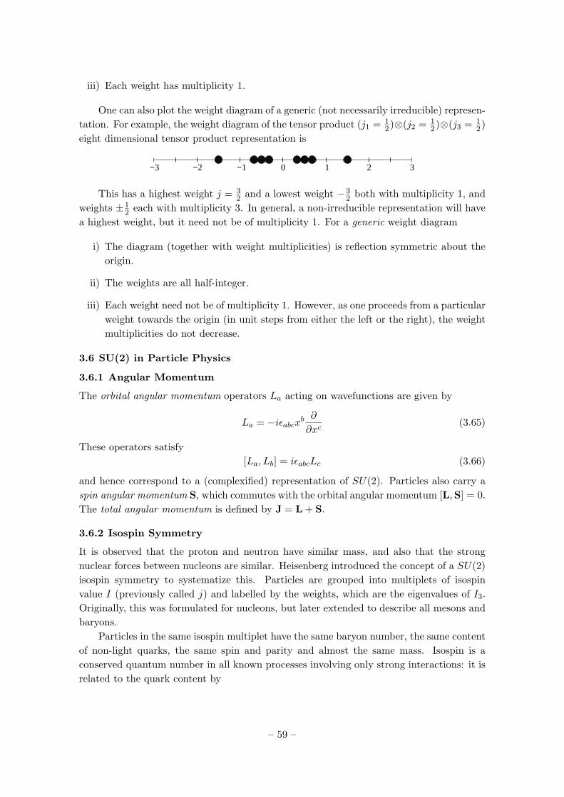
iii) Each weight has multiplicity 1.

One can also plot the weight diagram of a generic (not necessarily irreducible) represen-tation. For example, the weight diagram of the tensor product (j1 = 1

2)⊗(j2 = 12)⊗(j3 = 1

2)eight dimensional tensor product representation is

3210−1−2−3

This has a highest weight j = 32 and a lowest weight −3

2 both with multiplicity 1, andweights ±1

2 each with multiplicity 3. In general, a non-irreducible representation will havea highest weight, but it need not be of multiplicity 1. For a generic weight diagram

i) The diagram (together with weight multiplicities) is reflection symmetric about theorigin.

ii) The weights are all half-integer.

iii) Each weight need not be of multiplicity 1. However, as one proceeds from a particularweight towards the origin (in unit steps from either the left or the right), the weightmultiplicities do not decrease.

3.6 SU(2) in Particle Physics

3.6.1 Angular Momentum

The orbital angular momentum operators La acting on wavefunctions are given by

La = −iεabcxb∂

∂xc(3.65)

These operators satisfy[La, Lb] = iεabcLc (3.66)

and hence correspond to a (complexified) representation of SU(2). Particles also carry aspin angular momentum S, which commutes with the orbital angular momentum [L,S] = 0.The total angular momentum is defined by J = L + S.

3.6.2 Isospin Symmetry

It is observed that the proton and neutron have similar mass, and also that the strongnuclear forces between nucleons are similar. Heisenberg introduced the concept of a SU(2)isospin symmetry to systematize this. Particles are grouped into multiplets of isospinvalue I (previously called j) and labelled by the weights, which are the eigenvalues of I3.Originally, this was formulated for nucleons, but later extended to describe all mesons andbaryons.

Particles in the same isospin multiplet have the same baryon number, the same contentof non-light quarks, the same spin and parity and almost the same mass. Isospin is aconserved quantum number in all known processes involving only strong interactions: it isrelated to the quark content by

– 59 –

I3 =12

(N(u)−N(u)− (N(d)−N(d))) (3.67)

Isospin symmetry arises in the quark model because of the very similar properties ofthe u and d quarks.

Examples:

i) Nucleons have isospin I = 12 ; the proton has I3 = 1

2 , and the neutron has I3 = −12 :

n = |12,−1

2〉

p = |12,12〉 (3.68)

ii) The pions have I = 1 with

π− = |1,−1〉π0 = |1, 0〉π+ = |1, 1〉 (3.69)

iii) The strange baryons have I = 0 and I = 1

Σ− = |1,−1〉Σ0 = |1, 0〉Σ+ = |1, 1〉 (3.70)

and

Λ0 = |0, 0〉 (3.71)

iv) The strange mesons lie in two multiplets of I = 12

K0 = |12,−1

2〉

K+ = |12,12〉 (3.72)

and

K− = |12,−1

2〉

K0 = |12,12〉 (3.73)

K± are antiparticles with the same mass, but are in different isospin multipletsbecause of their differing quark content.

– 60 –

v) The light quarks have I = 12

d = |12,−1

2〉

u = |12,12〉 (3.74)

and all other quarks are isospin singlets I = 0.

3.6.3 Pauli’s Generalized Exclusion Principle and the Deuteron

Consider first NN nucleon-nucleon bound states. From the previously obtained decompo-sition of the (I1 = 1/2)⊗ (I2 = 1/2) tensor product we find the following isospin states

|1, 1〉 = pp, |1, 0〉 =1√2

(np+ pn), |1,−1〉 = nn (3.75)

which are are symmetric under exchange of isospin degrees of freedom, and the remainingstate is

|0, 0〉 =1√2

(np− pn) (3.76)

which is anti-symmetric under exchange of isospin degrees of freedom.The deuteron d is a pn bound state, which has no pp or nn partners. There is therefore

only one possibility; d = |0, 0〉.In general, the total wavefunction for a NN state can be written as a product of space,

spin, and isospin functions

ψ = ψ(space)ψ(spin)ψ(isospin) (3.77)

The generalized Pauli exclusion principle requires allowed NN wave-functions be anti-symmetric under exchange of all degrees of freedom. As ψ(isospin) is anti-symmetric,ψ(space)ψ(spin) must be symmetric- in fact ψ(space) is symmetric (the nucleons in the dare in a ` = 0 angular momentum state), and ψ(spin) as also symmetric, as d is a spin 1particle.

3.6.4 Pion-Nucleon Scattering and Resonances

Isospin can be used to investigate scattering processes; consider for example pion-nucleonscattering processes. From the decomposition of the (I1 = 1)⊗ (I2 = 1/2) tensor productwe find

|32,32〉 = π+p

|32,12〉 =

√23π0p+

1√3π+n

|32,−1

2〉 =

1√3π−p+

√23π0n

– 61 –

|32,−3

2〉 = π−n (3.78)

and

|12,12〉 =

1√3π0p−

√23π+n

|12,−1

2〉 =

√23π−p− 1√

3π0n (3.79)

These equations can be inverted to give

π+p = |32,32〉

π0p =

√23|32,12〉+

1√3|12,12〉

π+n =1√3|32,12〉 −

√23|12,12〉

π−p =1√3|32,−1

2〉+

√23|12,−1

2〉

π0n =

√23|32,−1

2〉 − 1√

3|12,−1

2〉

π−n = |32,−3

2〉 (3.80)

Consider πN scattering. The scattering is described by a S-matrix, which, in processesdominated by strong interactions is taken to be isospin invariant: [Ij , S] = 0 and so bySchur’s lemma

〈I ′,m′|S |I,m〉 = φ(I)δII′δmm′ (3.81)

The cross sections of the scattering processes are given by

σ(in→ out) = K| 〈in|S |out〉 |2 (3.82)

for constant K. Hence

σ(π+p→ π+p) = K|φ(32

)|2 (3.83)

σ(π0n→ π−p) =29K|φ(

32

)− φ(12

)|2 (3.84)

σ(π−p→ π−p) =19K|φ(

32

) + 2φ(12

)|2 (3.85)

For all three of these processes, a marked resonance is measured at approximately 1236Mev. The ratio of the cross-sections of these resonances is

σ(π+p→ π+p) : σ(π0n→ π−p) : σ(π−p→ π−p) = 1 :29

:19

(3.86)

which is consistent with the supposition that the resonance corresponds to a particle ofisospin 3

2 (and so |φ(32)| |φ(1

2)|). This particle is the ∆ particle, which lies in anisospin I = 3

2 multiplet with states ∆−, ∆0, ∆+, ∆++ having weights I3 = −32 ,−

12 ,

12 ,

32

respectively.

– 62 –

3.7 The semi-simplicity of (complexified) L(SU(n+ 1))

To proceed, define the n+ 1× n+ 1 square matrices Eij by (Ei,j)pq = δipδjq. Recall thatL(SU(n+1)) consists of the traceless antihermitian matrices, and is therefore spanned overR by i(Ei,i − En+1,n+1) for i = 1, . . . , n and Ei,j − Ej,i, i(Ei,j + Ej,i) for i < j. Hence, oncomplexification, the Lie algebra is spanned by traceless diagonal matrices together withthe Ei,j for i 6= j.

Suppose that h = diag (a1, a2, . . . , an+1),∑ai = 0 is a traceless diagonal matrix.

Then if i 6= j, observe that [h,Ei,j ] = (ai − aj)Ei,j .

Proposition 25. Complexified L(SU(n+ 1)) is semi-simple.Proof

Note by direct computation that

[Ei,j , Er,s] = δjrEi,s − δisEr,j (3.87)

so(ad Ep,q ad Ei,j)Er,s = δjrδiqEp,s − δjrδpsEi,q − δisδqrEp,j + δisδpjEr,q (3.88)

and hence the component of (ad Ep,q ad Ei,j)Er,s in the E`,t direction is

δjrδiqδp`δst − δjrδpsδi`δqt − δisδqrδp`δjt + δisδpjδr`δqt (3.89)

There are various cases to consider

i) κ(Ep,q, Ei,j) for p 6= q, i 6= j. We must compute Tr (ad Ep,q ad Ei,j). If r 6= s thenthe component of (ad Ep,q ad Ei,j)Er,s in the Er,s direction is

δjrδiqδpr − δjrδpsδirδqs − δisδqrδprδjs + δisδpjδqs = δjrδiqδpr + δisδpjδqs (3.90)

(as i 6= j and p 6= q). So the contribution to the trace from these terms is

n+1∑r=1,s=1,r 6=s

δjrδiqδpr + δisδpjδqs = 2nδiqδpj (3.91)

We also compute the component of (ad Ep,q ad Ei,j)Er,s in the direction Ek,k −En+1,n+1 for k = 1, . . . , n. Observe that the component of δiqEp,s − δpsEiq in thisdirection is δiqδps(δpk − δik) (if i 6= q or p 6= s then the diagonal components ofδiqEp,s−δpsEiq vanish). Hence the component of (ad Ep,q ad Ei,j)Er,s in the directionEk,k − En+1,n+1 for k = 1, . . . , n is

δjrδiqδps(δpk − δik) + δisδpjδrq(δrk − δpk) (3.92)

It follows that the component of (ad Ep,q ad Ei,j)(Ek,k − En+1,n+1) along (Ek,k −En+1,n+1) is

δjkδiqδpk(δpk − δik) + δikδpjδqk(1− δpk)

– 63 –

−(δj,n+1δiqδp,n+1(δpk − δik)− δi,n+1δpjδq,n+1δpk

)(3.93)

which can be simplified using i 6= j and p 6= q to

δjkδiqδpk + δikδpjδqk + δj,n+1δiqδp,n+1δik + δi,n+1δpjδq,n+1δpk (3.94)

On taking the sum from k = 1, . . . , n this gives a contribution to the trace of

2δiqδpj (3.95)

and so

κ(Ep,q, Ei,j) = 2(n+ 1)δiqδpj (3.96)

ii) κ(Ep,q, h) for h = diag (a1, a2, . . . , an+1) with∑

i ai = 0 and p 6= q. The onlycontribution to the trace Tr (ad Ep,q ad h) comes from terms

(ad Ep,q ad h)Ei,j = ad Ep,q(ai − aj)Ei,j = (ai − aj)(δqiEp,j − δp,jEi,q) (3.97)

for i 6= j. The component of this matrix along the Ei,j direction is

(ai − aj)(δqiδpi − δp,jδq,j) = 0 (3.98)

as p 6= q. Hence

κ(Ep,q, h) = 0 (3.99)

iii) κ(h, g) where h = diag (a1, a2, . . . , an+1) and g = diag (b1, b2, . . . , bn+1) and∑

i ai =∑i bi = 0,

The only contribution to the trace Tr (ad h ad g) is from the terms

(ad h ad g)Ei,j (3.100)

for i 6= j. But(ad h ad g)Ei,j = (ai − aj)(bi − bj)Ei,j (3.101)

so taking the sum over i and j (i 6= j) we obtain

κ(h, g) = 2(n+ 1)∑i

aibi (3.102)

Hence κ is negative definite over the span over R of i(Er,r−En+1,n+1) for r = 1, . . . , n;and this span is orthogonal to the span of the Ei,j − Ej,i and i(Ei,j + Ej,i) (i 6= j).Furthermore, κ is diagonal and negative definite over the span over R of the Ei,j−Ej,i andi(Ei,j + Ej,i). κ is therefore non-degenerate.

We also have the immediate corollory:

Corollory 2. The Lie algebra of SU(n+ 1) (as a real Lie algebra) is compact.

– 64 –

4. SU(3) and the Quark Model

The Lie algebra of SU(3) consists of the traceless antihermitian 3 × 3 complex matrices.It is convenient to define the following matrices

h1 =

12 0 00 −1

2 00 0 0

h2 =

1

2√

30 0

0 12√

30

0 0 − 1√3

e1

+ =

0 1√2

0

0 0 00 0 0

e1− =

0 0 01√2

0 0

0 0 0

e2

+ =

0 0 00 0 1√

2

0 0 0

e2− =

0 0 00 0 00 1√

20

e3

+ =

0 0 1√2

0 0 00 0 0

e3− =

0 0 00 0 01√2

0 0

(4.1)

Then ih1, ih2 and i(em+ +em− ), em+−em− for m = 1, 2, 3 form a basis for the antihermitiantraceless 3 × 3 matrices (over R), and hence are a basis for L(SU(3)). Suppose that d isthe irreducible representation of L(SU(3)) acting on a complex vector space V which isinduced from an irreducible representation of SU(3) acting on V .

It is convenient to set

H1 = d(h1), H2 = d(h2), Em± = d(em± ) for m = 1, 2, 3 (4.2)

Then we find the following commutators:

[H1, H2] = 0

[H1, E1±] = ±E1

±, [H1, E2±] = ∓1

2E2±, [H1, E

3±] = ±1

2E3±

[H2, E1±] = 0, [H2, E

2±] = ±

√3

2E2±, [H2, E

3±] = ±

√3

2E3± (4.3)

and

[E1+, E

1−] = H1

[E2+, E

2−] =

√3

2H2 −

12H1

[E3+, E

3−] =

√3

2H2 +

12H1 (4.4)

The remaining commutation relations are

[E1+, E

2+] =

1√2E3

+, [E1−, E

2−] = − 1√

2E3−

– 65 –

[E1+, E

3−] = − 1√

2E2−, [E1

−, E3+] =

1√2E2

+

[E2+, E

3−] =

1√2E1−, [E2

−, E3+] = − 1√

2E1

+ (4.5)

and

[E1+, E

2−] = [E1

−, E2+] = [E1

+, E3+] = [E1

−, E3−] = [E2

+, E3+] = [E2

−, E3−] = 0 (4.6)

Note in particular that H1, H2 commute. The subalgebra of L(SU(3)) spanned byih1 and ih2 is called the Cartan subalgebra. It is the maximal commuting subalgebra ofL(SU(3)).

4.1 Raising and Lowering Operators: The Weight Diagram

The Lie algebra of L(SU(3)) can be used to obtain three sets of L(SU(2)) algebras. Inparticular, we find that

[H1, E1±] = ±E1

±, [E1+, E

1−] = H1 (4.7)

and

[√

32H2 −

12H1, E

2±] = ±E2

±, [E2+, E

2−] =

√3

2H2 −

12H1 (4.8)

and

[√

32H2 +

12H1, E

3±] = ±E3

±, [E3+, E

3−] =

√3

2H2 +

12H1 (4.9)

In particular, there are three pairs of raising and lowering operators Em± .For simplicity, consider a representation d of L(SU(3)) obtained from a unitary repre-

sentation D of SU(3) such that d is an anti-hermitian representation- so that H1 and H2

are hermitian, and hence diagonalizable with real eigenvalues. Hence, H1 and√

32 H2± 1

2H1,can be simultaneously diagonalized, and the eigenvalues are real. (In fact the same can beshown without assuming unitarity!)

Suppose then that |φ〉 is an eigenstate of H1 with eigenvalue p and also an eigenstateof H2 with eigenvalue q. It is convenient to order the eigenvalues as points in R2 withposition vectors (p, q) where p is the eigenvalue of H1 and q of H2. (p, q) is then referredto as a weight.

From the commutation relations we have the following properties

i) Either E1± |φ〉 = 0 or E1

± |φ〉 is an eigenstate of H1 and H2 with eigenvalue (p, q)±(1, 0)

ii) Either E2± |φ〉 = 0 or E2

± |φ〉 is an eigenstate with eigenvalue (p, q)± (−12 ,√

32 )

iii) Either E3± |φ〉 = 0 or E3

± |φ〉 is an eigenstate with eigenvalue (p, q)± (12 ,√

32 )

Moreover, from the properties of L(SU(2)) representations we know that

2p = m1,√

3q − p = m2,√

3q + p = m3 (4.10)

– 66 –

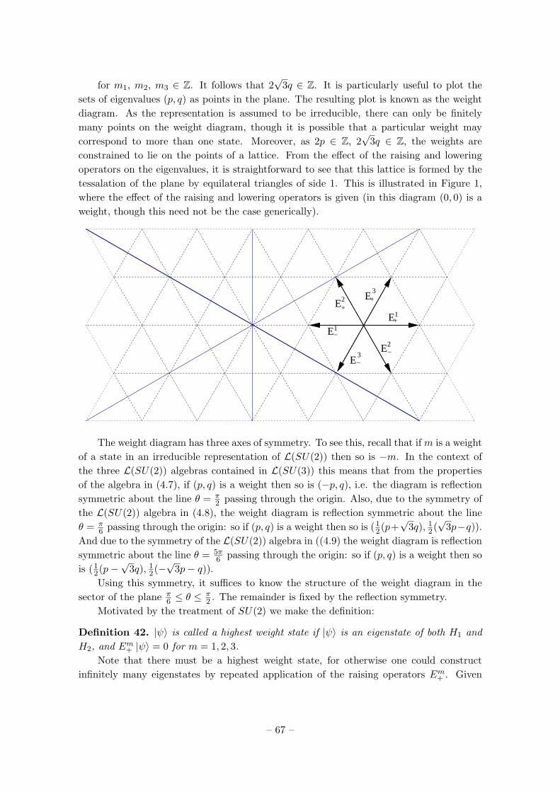
for m1, m2, m3 ∈ Z. It follows that 2√

3q ∈ Z. It is particularly useful to plot thesets of eigenvalues (p, q) as points in the plane. The resulting plot is known as the weightdiagram. As the representation is assumed to be irreducible, there can only be finitelymany points on the weight diagram, though it is possible that a particular weight maycorrespond to more than one state. Moreover, as 2p ∈ Z, 2

√3q ∈ Z, the weights are

constrained to lie on the points of a lattice. From the effect of the raising and loweringoperators on the eigenvalues, it is straightforward to see that this lattice is formed by thetessalation of the plane by equilateral triangles of side 1. This is illustrated in Figure 1,where the effect of the raising and lowering operators is given (in this diagram (0, 0) is aweight, though this need not be the case generically).

E1

E2

E3

E2

E1

E3

++

+

−

−

−

The weight diagram has three axes of symmetry. To see this, recall that if m is a weightof a state in an irreducible representation of L(SU(2)) then so is −m. In the context ofthe three L(SU(2)) algebras contained in L(SU(3)) this means that from the propertiesof the algebra in (4.7), if (p, q) is a weight then so is (−p, q), i.e. the diagram is reflectionsymmetric about the line θ = π

2 passing through the origin. Also, due to the symmetry ofthe L(SU(2)) algebra in (4.8), the weight diagram is reflection symmetric about the lineθ = π

6 passing through the origin: so if (p, q) is a weight then so is (12(p+

√3q), 1

2(√

3p−q)).And due to the symmetry of the L(SU(2)) algebra in ((4.9) the weight diagram is reflectionsymmetric about the line θ = 5π

6 passing through the origin: so if (p, q) is a weight then sois (1

2(p−√

3q), 12(−√

3p− q)).Using this symmetry, it suffices to know the structure of the weight diagram in the

sector of the plane π6 ≤ θ ≤

π2 . The remainder is fixed by the reflection symmetry.

Motivated by the treatment of SU(2) we make the definition:

Definition 42. |ψ〉 is called a highest weight state if |ψ〉 is an eigenstate of both H1 andH2, and Em+ |ψ〉 = 0 for m = 1, 2, 3.

Note that there must be a highest weight state, for otherwise one could constructinfinitely many eigenstates by repeated application of the raising operators Em+ . Given

– 67 –

a highest weight state, let V ′ be the vector space spanned by |ψ〉 and states obtained byacting with all possible products of lowering operators Em− on |ψ〉. As there are only finitelymany points on the weight diagram, there can only be finitely many such terms. Then, bymaking use of the commutation relations, it is clear that V ′ is an invariant subspace of V .As the representation is irreducible on V , this implies that V ′ = V , i.e. V is spanned by|ψ〉 and a finite set of states obtained by acting with lowering operators on |ψ〉. Supposethat (p, q) is the weight of |ψ〉. Then V is spanned by a basis of eigenstates of H1 and H2

with weights confined to the sector given by π ≤ θ ≤ 5π3 relative to (p, q)- all points on the

weight diagram must therefore lie in this sector.

Lemma 6. The highest weight state is unique.

Proof Suppose that |ψ〉 and |ψ′〉 are two highest weight states with weights (p, q), (p′, q′)respectively. Then (p′, q′) must make an angle π ≤ θ ≤ 5π

3 relative to (p, q) and (p, q) mustmake an angle π ≤ θ ≤ 5π

3 relative to (p′, q′). This implies that p = p′, q = q′.

Next suppose that |ψ1〉 and |ψ2〉 are two linearly independent highest weight states(both with weight (p, q)). Let V1 and V2 be the vector spaces spanned by the statesobtained by acting with all possible products of lowering operators Em− on |ψ1〉 and |ψ2〉respectively; one therefore obtains bases for V1 and V2 consisting of eigenstates of H1 andH2. By the reasoning given previously, as V1 and V2 are invariant subspaces of V and therepresentation is irreducible on V , it must be the case that V1 = V2 = V . In particular, wefind that |ψ2〉 ∈ V1. However, the only basis element of V1 which has weight (p, q) is |ψ1〉,hence we must have |ψ2〉 = c |ψ1〉 for some constant c, in contradiction to the assumptionthat |ψ1〉 and |ψ2〉 are linearly independent.

Having established the existence of a unique highest weight state |ψ〉, we can proceedto obtain the generic form for the weight diagram. Recall that the highest weight j of anirreducible representation of L(SU(2)) is always non-negative. By acting on |ψ〉 with thelowering operators Em− , one obtains three irreducible representations of L(SU(2)). Non-negativity of the highest weight corresponding to the L(SU(2)) irreducible representationgenerated by E1

− implies that the highest weight must lie in the half-plane to the right ofthe line θ = π

2 , or on the line θ = π2 :

Non-negativity of the highest weight corresponding to the L(SU(2)) irreducible represen-tation generated by E2

− implies that the highest weight must lie in the half-plane abovethe line θ = π

6 , or on the line θ = π6 :

– 68 –

Finally, non-negativity of the highest weight corresponding to the L(SU(2)) irreduciblerepresentation generated by E3

− implies that the highest weight must lie in the half-planeabove the line θ = 5π

6 , or on the line θ = 5π6 :

As the highest weight must lie in all three of these regions, it must lie in the sectorπ6 ≤ θ ≤

π2 relative to (0, 0), or at the origin:

Lemma 7. If the highest weight is (0, 0), then there is only one state in the representation,which is called the singlet.Proof

Let |ψ〉 be the highest weight state with weight (0, 0). Suppose that Em− |ψ〉 6= 0 forsomem. Then by the reflection symmetry of the weight diagram, it follows that Em+ |ψ〉 6= 0,in contradiction to the fact that Ei+ |ψ〉 = 0 for i = 1, 2, 3, as |ψ〉 is the highest weightstate. Hence Em± |ψ〉 = 0 for m = 1, 2, 3. Also H1 |ψ〉 = H2 |ψ〉 = 0. It follows that the1-dimensional subspace V ′ spanned by |ψ〉 is an invariant subspace of V , and thereforeV = V ′ as the representation is irreducible.

There are then three possible locations for the highest weight state |ψ〉.

4.1.1 Triangular Weight Diagrams (I)

Suppose that the highest weight lies on the line θ = π2 . In this case, by applying powers of

E2− the states of the L(SU(2)) representation given in (4.8) are generated. These form a

line orthogonal to the axis of reflection θ = π6 , about which they are symmetric, and there

– 69 –

are no states outside this line, as these points cannot be reached by applying loweringoperators. Then, by using the reflection symmetry, it follows that the outermost statesfrom an equilateral triangle with horizontal base. Each lattice point inside the trianglecorresponds to (at least) one state which has this weight, because each lattice point in thetriangle lies at some possible weight within the L(SU(2)) representation given in (4.7),and from the properties of L(SU(2)) representations, we know that this has a state withthis weight (i.e. as the L(SU(2)) weight diagram has no “holes” in it, neither does theL(SU(3)) weight diagram).

This case is illustrated by

Proposition 26. Each weight in this triangle corresponds to a unique state.Proof

Note that all of the states on the right edge of the triangle correspond to unique states,because these weights correspond to states which can only be obtained by acting on |ψ〉with powers of E2

−. It therefore follows by the reflection symmetry that all of the states onthe edges of the triangle have multiplicity one.

Now note the commutation relation

[E1−, E

2−] = − 1√

2E3− (4.11)

This implies that products of lowering operators involving E3− can be rewritten as

linear combinations of products of operators involving only E1− and E2

− (in some order).In particular, we find

(E1−)(E2

−)n |ψ〉 = [E1−, E

2−](E2

−)n−1 |ψ〉+ E2−E

1−(E2

−)n−1 |ψ〉

= − 1√2E3−(E2

−)n−1 |ψ〉+ E2−E

1−(E2

−)n−1 |ψ〉. . .

– 70 –

= − n√2E3−(E2

−)n−1 |ψ〉 (4.12)

by simple induction, where we have used the fact that E1− |ψ〉 = 0 and [E2

−, E3−] = 0.

A generic state of some fixed weight in the representation can be written as a linearcombination of products of E2

− and E1− lowering operators acting on |ψ〉 of the form

Π(E1−, E

2−) |ψ〉 (4.13)

where Π(E1−, E

2−) contains m powers of E2

− and ` powers of E1− where m, ` are uniquely

determined by the weight of the state- only the order of the operators is unfixed.

Using (4.12), commute the E1− states in this product to the right as far as they will

go. Then either one finds that the state vanishes (due to an E1− acting directly on |ψ〉), or

one can eliminate all of the E1− terms and is left with a term proportional to

(E2−)m−`(E3

−)` |ψ〉 (4.14)

where we have used the commutation relations [E2−, E

3−] = [E1

−, E3−] = 0.

Hence, it follows that all weights in the diagram can have at most multiplicity 1.However, from the property of the L(SU(2)) representations, as the weights in the outerlayers have multiplicity 1, it follows that all weights in the interior have multiplicity atleast 1.

Hence, all the weights must be multiplicity 1.

4.1.2 Triangular Weight Diagrams (II)

Suppose that the highest weight lies on the line θ = π6 . In this case, by applying powers of

E1− the states of the L(SU(2)) representation given in (4.7) are generated. These form a

horizontal line orthogonal to the axis of reflection θ = π2 , about which they are symmetric,

and there are no states outside this line, as these points cannot be reached by applyinglowering operators. Then, by using the reflection symmetry, it follows that the outermoststates from an inverted equilateral triangle with horizontal upper edge. Each lattice pointinside the triangle corresponds to (at least) one state which has this weight, because eachlattice point in the triangle lies at some possible weight within the L(SU(2)) representationgiven in (4.7), and from the properties of L(SU(2)) representations, we know that this hasa state with this weight (i.e. as the L(SU(2)) weight diagram has no “holes” in it, neitherdoes the L(SU(3)) weight diagram).

This case is illustrated by

– 71 –

Proposition 27. Each weight in this triangle corresponds to a unique state.Proof

Note that all of the states on the horizontal top edge of the triangle correspond tounique states, because these weights correspond to states which can only be obtained byacting on |ψ〉 with powers of E1

−. It therefore follows by the reflection symmetry that allof the states on the edges of the triangle have multiplicity one.

Now, using (4.11) it is straightforward to show that

E2−(E1

−)n |ψ〉 =n√2E3−(E1

−)n−1 |ψ〉 (4.15)

for n ≥ 1, where we have used E2− |ψ〉 = 0.

Now consider a state of some fixed weight in the representation; this can be written asa linear combination of terms of the form

Π(E1−, E

2−) |ψ〉 (4.16)

where Π(E1−, E

2−) contains m powers of E1

− and ` powers of E2− in an appropriate order,

where m and ` are determined uniquely by the weight of the state in question.Using (4.15), commute the E2

− states in this product to the right as far as they willgo. Then either one finds that the state vanishes (due to an E2

− acting directly on |ψ〉), orone can eliminate all of the E1

− terms and is left with a term proportional to

(E1−)m−`(E3

−)` |ψ〉 (4.17)

where we have used the commutation relations [E2−, E

3−] = [E1

−, E3−] = 0.

Hence, it follows that all weights in the diagram can have at most multiplicity 1.However, from the property of the L(SU(2)) representations, as the weights in the outerlayers have multiplicity 1, it follows that all weights in the interior have multiplicity atleast 1.

Hence, all the weights must be multiplicity 1.

– 72 –

4.1.3 Hexagonal Weight Diagrams

Suppose that the highest weight lies in the sector π6 < θ < π

2 . In this case, by applyingpowers of E1

− the states of the L(SU(2)) representation given in (4.7) are generated. Theseform a horizontal line extending to the left of the maximal weight which is orthogonalto the line θ = π

2 , about which they are symmetric, There are no states above, as thesepoints cannot be reached by applying lowering operators. Also, by applying powers of E2

−the states of the L(SU(2)) representation given in (4.8) are generated. These form a lineextending to the right of the maximal weight which is orthogonal to the axis of reflectionθ = π

6 , about which they are symmetric, and there are no states to the right of this line,as these points cannot be reached by applying lowering operators.

Then, by using the reflection symmetry, it follows that the outermost states form ahexagon. Each lattice point inside the hexagon corresponds to (at least) one state whichhas this weight, because each lattice point in the hexagon lies at some possible weightwithin the L(SU(2)) representation given in (4.7), and from the properties of L(SU(2))representations, we know that this has a state with this weight (i.e. as the L(SU(2)) weightdiagram has no “holes” in it, neither does the L(SU(3)) weight diagram).

This case is illustrated by

The multiplicities of the states for these weight diagrams are more complicated thanfor the triangular diagrams. In particular, the weights on the two edges of the hexagonleading off from the highest weight have multiplicity 1, because these states can only beconstructed as (E1

−)n |ψ〉 or (E2−)m |ψ〉. So by symmetry, all of the states on the outer layer

of the hexagon have multiplicity 1. However, if one proceeds to the next layer, then themultiplicity of all the states increases by 1. This happens until the first triangular layer isreached, at which point all following layers have the same multiplicity as the first triangularlayer.

– 73 –

Suppose that the top horizontal edge leading off the maximal weight is of length m,and that the other outer edge is of length n, with m ≥ n. This situation is illustratedbelow

n

m

The highest weight is then at (m2 ,1

2√

3(m + 2n)). The outer n layers are hexagonal,

whereas the n + 1-th layer is triangular, and all following layers are also triangular. Asone goes inwards through the outer n+ 1 layers the multiplicity of the states in the layersincreases from 1 in the first outer layer to n+ 1 in the n+ 1-th layer. Then all the statesin the following triangular layers have multiplicity n+ 1 as well.

We will prove this in several steps.

Proposition 28. States with weights on the k-th hexagonal layer for k = 1, . . . , n or thek = n+ 1-th layer (the first triangular layer) have multiplicity not exceeding k.Proof

In order to prove this, consider first a state on the upper horizontal edge of the k-thlayer for k ≤ n + 1. The length of this edge is m − k + 1. A general state on this edge isobtained via

Π(E2−, E

1−) |ψ〉 (4.18)

where Π(E2−, E

1−) contains (in some order) k − 1 powers of E2

− and ` powers of E1− for

` = k − 1, . . . ,m.Now use the commutation relation (4.11) to commute the powers of E2

− to the right asfar as they will go. Then the state can be written as a linear combination of the k vectors

|vi〉 = (E3−)i−1(E1

−)`−i+1(E2−)k−i |ψ〉 (4.19)

for i = 1, . . . , k.It follows that this state has multiplicity ≤ k.

– 74 –

Next consider a state again on the k-th level, but now on the edge leading off to theright of the horizontal edge which we considered above; this edge is parallel to the outeredge of length n. Take k ≤ n+ 1, so the edge has length n− k+ 1. A state on this edge isobtained via

Π(E1−, E

2−) |ψ〉 (4.20)

where Π(E1−, E

2−) contains (in some order) k − 1 powers of E1

− and ` powers of E2− where

` = k − 1, . . . , n. Now use the commutation relation (4.11) to commute the powers of E1−

to the right as far as they will go. Then the state can be written as a linear combinationof the k vectors

|wi〉 = (E3−)i−1(E2

−)`−i+1(E1−)k−i |ψ〉 (4.21)

for i = 1, . . . , k.So these states also have multiplicity ≤ k. By using the reflection symmetry, it follows

that the all the states on the k-th hexagonal layer have multiplicity k. We also have the

Proposition 29. The states with weights in the triangular layers have multiplicity notexceeding n+ 1.Proof

Consider a state on the k-th row of the weight diagram for m+ 1 ≥ k ≥ n+ 1 whichlies inside the triangular layers. Such a state can also be written as

Π(E2−, E

1−) |ψ〉 (4.22)

where Π(E2−, E

1−) contains (in some order) k − 1 powers of E2

− and ` powers of E1− for

` = k − 1, . . . ,m. and hence by the reasoning above, it can be rewritten as a linearcombination of the k vectors |vi〉 in (4.19), however for i < k−n, |vi〉 = 0 as (E2

−)k−i |ψ〉 = 0.The only possible non-vanishing vectors are the n + 1 vectors |vk−n〉 , |vk−n+1〉 , . . . , |vk〉.Hence these states have multiplicity ≤ n+ 1.

Next note the lemma

Lemma 8. Define |wi,k〉 = (E3−)i−1(E1

−)k−i(E2−)k−i |ψ〉 for i = 1, . . . , k, k = 1, . . . , n+ 1.

Then the sets Sk = |w1,k〉 , . . . , |wk,k〉 are linearly independent for k = 1, . . . , n+ 1.Proof

By using the commutation relations, it is straightforward to prove the identities

E3+ |wi,k〉 = (i− 1)

(√32q +

12p+

i

2+ 1− k

)|wi−1,k−1〉

− 1√2

(k − i)2(√3

2q − 1

2p+

i

2+

12− k

2|wi,k−1〉

E2+ |wi,k〉 = E1

−( 1√

2(i− 1) |wi−1,k−1〉

+ (k − i)(√3

2q − 1

2p− 1

2(k − i− 1)

)|wi,k−1〉

)(4.23)

(with obvious simplifications in the cases when i = 1 or i = k)

– 75 –

Note that S1 = |ψ〉 is linearly independent. Suppose that Sk−1 is linearly indepen-dent (k ≥ 2). Consider Sk. Suppose

k∑i=1

ci |wi,k〉 = 0 (4.24)

for some constants ci. Applying E3+ to (4.24) and using the linear independence of

Sk−1 we find the relation

i(√

32

+12p+

i

2+

32− k)ci+1 −

1√2

(k − i)2(√

32q − 1

2p+

i

2+

12− 1

2k)ci = 0 (4.25)

for i = 1, . . . , k − 1. Applying E2+ to (4.24) another recursion relation is obtained

1√2ici+1 + (k − i)(

√3

2q − 1

2p+

i

2+

12− 1

2k)ci = 0 (4.26)

Combining these relations we find ci+1 = 0 for i = 1, . . . , k−1. If√

32 q−

12p+ i

2 + 12−

12k 6= 0

when i = 1 then one also has c1 = 0. This holds if k ≤ n+ 1, however if k = n+ 2 then c1

is not fixed by these equations. The induction stops at this point. These results are sufficient to fix the multiplicity of all the states. This is because the

vectors in Sk for 1 ≤ k ≤ k + 1 correspond to states with weight (p, q) − (k − 1)(12 ,√

32 )

which are at the top right hand corner of the k-th hexagonal (or outermost triangular fork = n + 1) layer. We have shown therefore that these weights have multiplicity both lessthan or equal to, and greater than or equal to k. Hence these weights have multiplicityk. Next consider the states on the level k edges which are obtained by acting with theL(SU(2)) lowering operators E1

− and E2− on the “corner weight” states. Observe the

following:

Lemma 9. Let d be a representation of L(SU(2)) on V be such that a particular L(SU(2))weight m > 0 has multiplicity p. Then all weights m′ such that |m′| ≤ m have multiplicity≥ p

whose proof is left as an exercise.By this lemma, all the states on the k-th layer obtained in this fashion have multi-

plicity k also. Then the reflection symmetry implies that all states on the k-th layer havemultiplicity k.

In particular, the states on the outer triangular layer have multiplicity n + 1. Wehave shown that the states on the triangular layers must have multiplicity not greater thann+ 1, but by the lemma above together with the reflection symmetry, they must also havemultiplicity ≥ n + 1. Hence the triangular layer weights have multiplicity n + 1, and theproof is complete.

This was rather long-winded. There exist general formulae constraining multiplicitiesof weights in more general Lie group representations, but we will not discuss these here.

– 76 –

4.1.4 Dimension of Irreducible Representations

Using the multiplicity properties of the weight diagram, it is possible to compute thedimension of the representation. We consider first the hexagonal weight diagram for m ≥ n.

Then there are 1+ · · ·+(m−n)+(m−n+1) = 12(m−n+1)(m−n+2) weights in the

interior triangle. Each of these weights has multiplicity (n+ 1) which gives 12(n+ 1)(m−

n + 1)(m − n + 2) linearly independent states corresponding to weights in the triangle.Consider next the k-th hexagonal layer for k = 1, . . . , n. This has 3((m + 1 − (k − 1)) +(n+ 1− (k − 1))− 2) = 3(m+ n+ 2− 2k) weights in it, and each weight has multiplicityk, which gives 3k(m+ n+ 2− 2k) linearly independent states in the k-th hexagonal layer.

The total number of linearly independent states is then given by

12

(n+1)(m−n+1)(m−n+2)+n∑k=1

3k(m+n+2−2k) =12

(m+1)(n+1)(m+n+2) (4.27)

This formula also applies in the case for m ≤ n and also for the triangular weight diagramsby taking m = 0 or n = 0. The lowest dimensional representations are therefore 1,3,6,8,10...

4.1.5 The Complex Conjugate Representation

Definition 43. Let d be a representation of a Lie algebra L(G) acting on V . If v ∈ L(G),then viewing d(v) as a matrix acting on V , the complex representation d is defined by

d(v)u = (d(v))∗u (4.28)

for u ∈ V , where ∗ denotes matrix complex conjugation.Note that as d(v) is linear in v over R, it follows that (d(v))∗ is also linear in v over

R. Also, asd([v, w]) = d(v)d(w)− d(w)d(v) (4.29)

for v, w ∈ L(G), so taking the complex conjugate of both sides we find

d([v, w]) = d(v)d(w)− d(w)d(v) (4.30)

i.e. d is indeed a Lie algebra representation.Suppose that Ta are the generators of L(G) with structure constants cabc. Then as d

is a representation,[d(Ta), d(Tb)] = cab

cd(Tc) (4.31)

Taking the complex conjugate, and recalling that cabc are real, we find

[d(Ta), d(Tb)] = cabcd(Tc) (4.32)

i.e. the d(Ta) and d(Ta) satisfy the same commutation relations.In the context of representations of L(SU(3)), the conjugate operators to iH1, iH2,

i(Em+ +Em− ) and Em+ −Em− are denoted by iH1, iH2, i(Em− +Em+ ), and Em+ −Em− respectivelyand are given by

iH1 = (iH1)∗

– 77 –

iH2 = (iH2)∗

i(Em− + Em+ ) = (i(Em+ + Em− ))∗

Em+ − Em− = (Em+ − Em− )∗ (4.33)

which implies

H1 = −(H1)∗, H2 = −(H2)∗, Em± = −(Em∓ )∗ (4.34)

Then H1, H2 and Em± satisfy the same commutation relations as the unbarred opera-tors, and also behave in the same way under the hermitian conjugate. One can thereforeplot the weight diagram associated with the conjugate representation d, the weights beingthe (real) eigenvalues of H1 and H2. But as H1 = −(H1)∗ and H2 = −(H2)∗ it followsthat if (p, q) is a weight of the representation d, then (−p,−q) is a weight of the represen-tation d. So the weight diagram of d is obtained from that of d by inverting all the points(p, q) → −(p, q). Note that this means that the equilateral triangular weight diagrams Nand H of equal length sides are conjugate to each other.

4.2 Some Low-Dimensional Irreducible Representations of L(SU(3))

4.2.1 The Singlet

The simplest representation has only one state, which is the highest weight state withweight (0, 0). This representation is denoted 1.

4.2.2 3-dimensional Representations

Take the fundamental representation. Then as h1 and h2 are already diagonalized, it isstraightforward to compute the eigenstates and weights.

– 78 –

State Weight100

(12 ,

12√

3)

010

(−12 ,

12√

3)

001

(0,− 1√3)

The state of highest weight is

100

which has weight (12 ,

12√

3). The weight diagram is

d u

s

This representation is denoted 3. It will be convenient to define the following statesin the 3 representation.

u =

100

, d =

010

, s =

001

(4.35)

so that u has weight (12 ,

12√

3), d has weight (−1

2 ,1

2√

3) and s has weight (0,− 1√

3).

The lowering operators have the following effect: d =√

2e1−u, s =

√2e3−u and s =√

2e2−d.The complex conjugate of this representation is called 3 and the weights are obtained

by multiplying the weights of the 3 representation by −1.

– 79 –

State Weight100

(−12 ,−

12√

3)

010

(12 ,−

12√

3)

001

(0, 1√3)

The state of highest weight is

001

which has weight (0, 1√3). The weight diagram is

s

u d

It will be convenient to define the following states in the 3 representation.

u =

100

, d =

010

, s =

001

(4.36)

so that u has weight (−12 ,−

12√

3), d has weight (1

2 ,−1

2√

3) and s has weight (0, 1√

3).

The lowering operators have the following effect: u = −√

2e3−s, d = −

√2e2−s and

u = −√

2e1−d; where em± = −(em∓ )∗.

Exercise: Verify that all other lowering operators em− (except those given above) an-nihilate u, d, s. Also compute the effect of the raising operators em+ .

– 80 –

4.2.3 Eight-Dimensional Representations

Consider the adjoint representation defined on the complexified Lie algebra L(SU(3)), i.e.ad(v)w = [v, w]. Then the weights of the states can be computed by evaluating thecommutators with h1 and h2:

State v [h1, v] [h2, v] Weighth1 0 0 (0, 0)h2 0 0 (0, 0)e1

+ e1+ 0 (1, 0)

e1− −e1

− 0 (−1, 0)e2

+ −12e

2+

√3

2 e2+ (−1

2 ,√

32 )

e2−

12e

2− −

√3

2 e2− (1

2 ,−√

32 )

e3+

12e

3+

√3

2 e3+ (1

2 ,√

32 )

e3− −1

2e3− −

√3

2 e3− (−1

2 ,−√

32 )

The highest weight state is e3+ with weight (1

2 ,√

32 ). All weights have multiplicity 1

except for (0, 0) which has multiplicity 2. The weight diagram is a regular hexagon:

4.3 Tensor Product Representations

Suppose that d1, d2 are irreducible representations of L(SU(3)) acting on V1, V2 respec-tively. Then let V = V1

⊗V2 and d = d1⊗ 1 + 1⊗ d2 be the tensor product representation

of L(SU(3)) on V . In general d is not irreducible on V , so we want to decompose V intoa direct sum of invariant subspaces on which the restriction of d is irreducible.

To do this, recall that one can choose a basis of V1 which consists entirely of eigenstatesof both d1(h1) and d1(h2). Similarly, one can also choose a basis of V2 which consists entirelyof eigenstates of both d2(h1) and d2(h2). Then the tensor product of the basis eigenstatesproduces a basis of V1

⊗V2 which consists of eigenstates of d(h1) and d(h2).

Explicitly, suppose that |φi〉 ∈ Vi is an eigenstate of di(h1) and di(h2) with weight(pi, qi) (i.e. di(h1) |φi〉 = pi |φi〉 and di(h2) |φi〉 = qi |φi〉) for i = 1, 2. Define |φ〉 =

– 81 –

|φ1〉 ⊗ |φ2〉. Then

d(h1) |φ〉 = (d1(h1) |φ1〉)⊗ |φ2〉+ |φ1〉 ⊗ (d2(h1) |φ2〉)= (p1 |φ1〉)⊗ |φ2〉+ |φ1〉 ⊗ (p2 |φ2〉)= (p1 + p2) |φ〉 (4.37)

and similarly

d(h2) |φ〉 = (q1 + q2) |φ〉 (4.38)

So the weight of |φ〉 is (p1 + p2, q1 + q2); the weights add in the tensor product repre-sentation.

Using this, one can plot a weight diagram consisting of the weights of all the eigenstatesin the tensor product basis of V , the points in the weight diagram are obtained by addingthe pairs of weights from the weight diagrams of d1 and d2 respectively, keeping carefultrack of the multiplicities (as the same point in the tensor product weight diagram may beobtained from adding weights from different states in V1

⊗V2.)

Once the tensor product weight diagram is constructed, pick a highest weight, whichcorresponds to a state which is annihilated by the tensor product operators Em+ for m =1, 2, 3. (Note that as the representation is finite-dimensional such a state is guaranteedto exist, though as the representation is no longer irreducible, it need not be unique). Ifthere are multiple highest weight states corresponding to the same highest weight, onecan without loss of generality take them to be mutually orthogonal. Picking one of these,generate further states by acting on a highest weight state with all possible combinationsof lowering operators. The span of these (finite number) of states produces an invariantsubspace W1 of V on which d is irreducible. Remove these weights from the tensor productweight diagram. If the multiplicity of one of the weights in the original tensor productdiagram is k, and the multiplicity of the same weight in the W1 weight diagram is k′ thenon removing the W1 weights, the multiplicity of that weight must be reduced from k tok − k′.

Repeat this process until there are no more weights left. This produces a decompositionV = W1

⊕...⊕Wk of V into invariant subspaces Wj on which d is irreducible.

Note that one could also perform this process on triple (and higher order) tensorproducts e.g. V1

⊗V2⊗V3. In this case, one would construct the tensor product weight

diagram by adding triplets of weights from the weight diagrams of d1 on V1, d2 on V2 andd3 on V3 respectively.

This process can be done entirely using the weight diagrams, because we have shownthat for irreducible representations, the location of the highest weight fixes uniquely theshape of the weight diagram and the multiplicities of its states.

We will see how this works for some simple examples:

4.3.1 3⊗ 3 decomposition.

Consider the 3⊗ 3 tensor product. Adding the weights together one obtains the followingtable of quark content and associated weights

– 82 –

Quark content and weights for 3⊗ 3

Quark Content Weight

u⊗ u (1, 1√3)

d⊗ d (−1, 1√3)

s⊗ s (0,− 2√3)

u⊗ d, d⊗ u (0, 1√3)

u⊗ s, s⊗ u (12 ,−

12√

3)

d⊗ s, s⊗ d (−12 ,−

12√

3)

Plotting the corresponding weight diagram gives

The raising and lowering operators are Em± = em± ⊗ 1 + 1 ⊗ em± . The highest weight stateis u ⊗ u with weight (1, 1√

3). Applying lowering operators to u ⊗ u it is clear that a

six-dimensional irreducible representation is obtained. The (unit-normalized) states andweights are given by

States and weights for the 6 in 3⊗ 3

State Weight

u⊗ u (1, 1√3)

d⊗ d (−1, 1√3)

s⊗ s (0,− 2√3)

1√2(d⊗ u+ u⊗ d) (0, 1√

3)

1√2(u⊗ s+ s⊗ u) (1

2 ,−1

2√

3)

1√2(d⊗ s+ s⊗ d) (−1

2 ,−1

2√

3)

– 83 –

which has the following weight diagram

This representation is called 6. Removing the (non-vanishing) span of these statesfrom the tensor product space, one is left with a 3-dimensional vector space. The newhighest weight is at (0, 1√

3) with corresponding state 1√

2(d⊗ u− u⊗ d) (this is the unique

linear combination- up to overall scale- of d⊗ u and u⊗ d which is annihilated by all theraising operators). This generates a 3. The states and their weights are

States and weights for the 3 in 3⊗ 3

State Weight1√2(d⊗ u− u⊗ d) (0, 1√

3)

1√2(d⊗ s− s⊗ d) (−1

2 ,−1

2√

3)

1√2(s⊗ u− u⊗ s) (1

2 ,−1

2√

3)

Hence 3 ⊗ 3 = 6 ⊕ 3. The states in the 6 are symmetric, whereas those in the 3 areantisymmetric.

4.3.2 3⊗ 3 decomposition

For this tensor product the quark content/weight table is as follows:

– 84 –

Quark content and weights for 3⊗ 3

Quark Content Weight

u⊗ s (12 ,√

32 )

u⊗ d (1, 0)

d⊗ s (−12 ,√

32 )

u⊗ u, d⊗ d, s⊗ s (0, 0)

d⊗ u (−1, 0)

s⊗ u (−12 ,−

√3

2 )

s⊗ d (12 ,−

√3

2 )

with weight diagram

ds us

du dd,uu,ss ud

su sd

The raising and lowering operators are Em± = em± ⊗ 1 + 1 ⊗ em± All weights havemultiplicity 1, except for (0, 0) which has multiplicity 3. The highest weight state is u⊗ swith weight (1

2 ,√

32 ). Acting on this state with all possible lowering operators one obtains

an 8 with the following states and weights

States and weights for the 8 in 3⊗ 3

State Weight

u⊗ s (12 ,√

32 )

u⊗ d (1, 0)

d⊗ s (−12 ,√

32 )

1√2(d⊗ d− u⊗ u), 1√

6(d⊗ d+ u⊗ u− 2s⊗ s) (0, 0)

d⊗ u (−1, 0)

s⊗ u (−12 ,−

√3

2 )

s⊗ d (12 ,−

√3

2 )

– 85 –

Removing these weights from the weight diagram, one is left with a singlet 1 withweight (0, 0), corresponding to the state

1√3

(u⊗ u+ s⊗ s+ d⊗ d) (4.39)

which is the unique linear combination- up to an overall scale- of u⊗u, s⊗ s and d⊗d whichis annihilated by the raising operators Em+ . Hence we have the decomposition 3⊗3 = 8⊕1.

4.3.3 3⊗ 3⊗ 3 decomposition.

For this tensor product the quark content/weight table is as follows:

Quark content and weights for 3⊗ 3⊗ 3

Quark Content Weight

u⊗ u⊗ u (32 ,√

32 )

s⊗ s⊗ s (0,−√

3)

d⊗ d⊗ d (−32 ,√

32 )

u⊗ u⊗ s, u⊗ s⊗ u, s⊗ u⊗ u (1, 0)

u⊗ u⊗ d, u⊗ d⊗ u, d⊗ u⊗ u (12 ,√

32 )

s⊗ s⊗ u, s⊗ u⊗ s, u⊗ s⊗ s (12 ,−

√3

2 )

s⊗ s⊗ d, s⊗ d⊗ s, d⊗ s⊗ s (−12 ,−

√3

2 )

d⊗ d⊗ s, d⊗ s⊗ d, s⊗ d⊗ d (−1, 0)

d⊗ d⊗ u, d⊗ u⊗ d, u⊗ d⊗ d (−12 ,√

32 )

u⊗ d⊗ s, u⊗ s⊗ d, d⊗ u⊗ s,d⊗ s⊗ u, s⊗ u⊗ d, s⊗ d⊗ u (0, 0)

with weight diagram

ddd ddu duu uuu

ddsdus

uus

dss uss

sss

The raising and lowering operators are Em± = em± ⊗ 1 ⊗ 1 + 1 ⊗ em± ⊗ 1 + 1 ⊗ 1 ⊗ em± .There are six weights of multiplicity 3, and the weight (0, 0) has multiplicity 6. The highest

– 86 –

weight is u⊗ u⊗ u with weight (32 ,√

32 ). By applying lowering operators to this state, one

obtains a triangular 10-dimensional irreducible representation denoted by 10, which hasnormalized states and weights:

States and weights for 10 in 3⊗ 3⊗ 3

State Weight

u⊗ u⊗ u (32 ,√

32 )

s⊗ s⊗ s (0,−√

3)

d⊗ d⊗ d (−32 ,√

32 )

1√3(u⊗ u⊗ s+ u⊗ s⊗ u+ s⊗ u⊗ u) (1, 0)

1√3(u⊗ u⊗ d+ u⊗ d⊗ u+ d⊗ u⊗ u) (1

2 ,√

32 )

1√3(s⊗ s⊗ u+ s⊗ u⊗ s+ u⊗ s⊗ s) (1

2 ,−√

32 )

1√3(s⊗ s⊗ d+ s⊗ d⊗ s+ d⊗ s⊗ s) (−1

2 ,−√

32 )

1√3(d⊗ d⊗ s+ d⊗ s⊗ d+ s⊗ d⊗ d) (−1, 0)

1√3(d⊗ d⊗ u+ d⊗ u⊗ d+ u⊗ d⊗ d) (−1

2 ,√

32 )

1√6(u⊗ d⊗ s+ u⊗ s⊗ d+ d⊗ u⊗ s+d⊗ s⊗ u+ s⊗ u⊗ d+ s⊗ d⊗ u) (0, 0)

The 10 weight diagram is

ddd ddu duu uuu

dds dus uus

dss uss

sss

Removing the (non-vanishing) span of these states from the tensor product space, oneis left with a 17-dimensional vector space. The new weight diagram is

– 87 –

ddu duu

ddsdus

uus

dss uss

Note that the highest weight is now (12 ,√

32 ). This weight has has multiplicity 2. It

should be noted that the subspace consisting of linear combinations of d⊗ u⊗ u, u⊗ d⊗ uand u ⊗ u ⊗ d which is annihilated by all raising operators Em+ is two-dimensional andis spanned by the two orthogonal states 1√

6(d ⊗ u ⊗ u + u ⊗ d ⊗ u − 2u ⊗ u ⊗ d) and

1√2(d ⊗ u ⊗ u − u ⊗ d ⊗ u). By acting on these two states with all possible lowering

operators, one obtains two 8 representations whose states are mutually orthogonal.

The states and weights of these two 8 representations are summarized below:

States and weights for an 8 in 3⊗ 3⊗ 3

State Weight1√6(d⊗ u⊗ u+ u⊗ d⊗ u− 2u⊗ u⊗ d) (1

2 ,√

32 )

1√6(s⊗ u⊗ u+ u⊗ s⊗ u− 2u⊗ u⊗ s) (1, 0)

1√6(2d⊗ d⊗ u− d⊗ u⊗ d− u⊗ d⊗ d) (−1

2 ,√

32 )

12√

3(s⊗ d⊗ u+ s⊗ u⊗ d+ d⊗ s⊗ u

+u⊗ s⊗ d− 2d⊗ u⊗ s− 2u⊗ d⊗ s),1

2√

3(2s⊗ d⊗ u+ 2d⊗ s⊗ u− s⊗ u⊗ d−d⊗ u⊗ s− u⊗ s⊗ d− u⊗ d⊗ s) (0, 0)1√6(s⊗ d⊗ d+ d⊗ s⊗ d− 2d⊗ d⊗ s) (−1, 0)

1√6(2s⊗ s⊗ u− s⊗ u⊗ s− u⊗ s⊗ s) (1

2 ,−√

32 )

1√6(2s⊗ s⊗ d− s⊗ d⊗ s− d⊗ s⊗ s) (−1

2 ,−√

32 )

– 88 –

States and weights for another 8 in 3⊗ 3⊗ 3

State Weight1√2(d⊗ u⊗ u− u⊗ d⊗ u) (1

2 ,√

32 )

1√2(s⊗ u⊗ u− u⊗ s⊗ u) (1, 0)

1√2(d⊗ u⊗ d− u⊗ d⊗ d) (−1

2 ,√

32 )

12(s⊗ d⊗ u+ s⊗ u⊗ d− d⊗ s⊗ u− u⊗ s⊗ d),12(s⊗ u⊗ d+ d⊗ u⊗ s− u⊗ s⊗ d− u⊗ d⊗ s) (0, 0)

1√2(s⊗ d⊗ d− d⊗ s⊗ d) (−1, 0)

1√2(s⊗ u⊗ s− u⊗ s⊗ s) (1

2 ,−√

32 )

1√2(s⊗ d⊗ s− d⊗ s⊗ s) (−1

2 ,−√

32 )

Removing these weights from the weight diagram, we are left with a singlet 1 withweight (0, 0). The state corresponding to this singlet is

1√6

(s⊗ d⊗ u− s⊗ u⊗ d+ d⊗ u⊗ s− d⊗ s⊗ u+ u⊗ s⊗ d− u⊗ d⊗ s) (4.40)

which is the only linear combination-up to overall scale- of u⊗ d⊗ s, u⊗ s⊗ d, d⊗ u⊗ s,d⊗ s⊗ u, s⊗ u⊗ d and s⊗ d⊗ u which is annihilated by all the raising operators.

Hence we have the decomposition 3⊗ 3⊗ 3 = 10⊕ 8⊕ 8⊕ 1 where the states in 10are symmetric, but the state in 1 is antisymmetric. The 8 states have mixed symmetry.

4.4 The Quark Model

It is possible to arrange the baryons and the mesons into SU(3) multiplets; i.e. the stateslie in Hilbert spaces which are tensor products of vector spaces equipped with irreduciblerepresentations of L(SU(3)). To see examples of this, it is convenient to group hadrons intomultiplets with the same baryon number and spin. We plot the hypercharge Y = S + B

where S is the strangeness and B is the baryon number against the isospin eigenvalue I3

for these particles.

4.4.1 Meson Multiplets

The pseudoscalar meson octet has B = 0 and J = 0. The (I3, Y ) diagram is

– 89 –

Y

I3

+ −

−

1/2

1

−1/2

−1

Mass(Mev)495

137

549

495

K K

K K0

0 +

π π π0

η−1 −1/2 1/2 1

There is also a J = 0 meson singlet η′.

The vector meson octet has B = 0 and J = 1. The (I3, Y ) diagram is

Y

I3

+ −

−

1/2

1

−1/2

−1

Mass(Mev)892

770

783

892

K K

K K0

0 +

0

∗ ∗

∗ ∗

ρ ρ ρ

ω−1 −1/2 1/2 1

There is also a J = 1 meson singlet, φ.

4.4.2 Baryon Multiplets

The baryon decuplet has B = 1 and J = 32 with (I3, Y ) diagram

– 90 –

Y

I3

1/2

1

−1/2

−1

−3/2

−2

∆ ∆ ∆ ∆

Σ Σ Σ

Ξ Ξ

Ω

+

+

++0

0

0

−

−

−

−

∗ ∗ ∗

∗ ∗

Mass (Mev)

1235

1385

1530

1670

−3/2 −1 −1/2 1/2 1 3/2

There is also an antibaryon decuplet with (I3, Y )→ −(I3, Y ).The baryon octet has B = 1, J = 1

2 with (I3, Y ) diagram

Y

I3

n p

Σ Σ

Ξ Ξ

+

+

Σ−

−

Λ

0

0

1/2

1

−1/2

−1

Mass(Mev)939

1193

1116

1318

−1/2 11/2−1

and there is also a J = 12 baryon singlet Λ0∗.

4.4.3 Quarks: Flavour and Colour

On making the identification (p, q) = (I3,√

32 Y ) the points on the meson and baryon octets

and the baryon decuplet can be matched to points on the weight diagrams of the 8 and 10of L(SU(3)).

Motivated by this, it is consistent to consider the (light) meson states as lying withina 3 ⊗ 3; as 3 ⊗ 3 = 8 ⊕ 1, the meson octets are taken to correspond to the 8 states, andthe meson singlets correspond to the singlet 1 states. The light baryon states lie within a3⊗ 3⊗ 3; the baryon decuplet corresponds to the 10 in 3⊗ 3⊗ 3 = 10⊕ 8⊕ 8⊕ 1; thebaryon octet corresponds to appropriate linear combinations of elements in the 8 irreps,and the baryon singlet corresponds to the 1.

– 91 –

In this model, the fundamental states in the 3 are quarks, with basis states u (up),d (down) and s (strange). The basis labels u, d, s are referred to as the flavours of thequarks. The 3 states are called antiquarks with basis u, d, s. Baryons are composed ofbound states of three quarks qqq, mesons are composed of bound states of pairs of quarksand antiquarks qq. The quarks have J = 1

2 and B = 13 whereas the antiquarks have J = 1

2

and B = −13 which is consistent with the values of B and J for the baryons and mesons.

The quark and antiquark flavours can be plotted on the (I3, Y ) plane:

Y

I3

1/3

−2/3

d u

s

−1/2 1/2I3−1/2 1/2

Y2/3

−1/3

s

u d

We have shown that mesons and baryons can be constructed from qq and qqq statesrespectively. But why do qq particles not exist? This problem is resolved using the notionof colour. Consider the ∆++ particle in the baryon decuplet. This is a u⊗u⊗u state withJ = 3

2 . The members of the decuplet are the spin 32 baryons of lowest mass, so we assume

that the quarks have vanishing orbital angular momentum. Then the spin J = 32 is obtained

by having all the quarks in the spin up state, i.e. u ↑ ⊗u ↑ ⊗u ↑. However, this violates thePauli exclusion principle. To get round this problem, it is conjectured that quarks possessadditional labels other than flavour. In particular, quarks have additional charges calledcolour charges- there are three colour basis states associated with quarks called r (red), g(green) and b (blue). The quark state wave-functions contain colour factors which lie ina 3 representation of SU(3) which describes their colour; the colour of antiquark statescorresponds to a 3 representation of SU(3) (colour). This colour SU(3) is independent ofthe flavour SU(3).

These colour charges are also required to remove certain discrepancies (of powers of3) between experimentally observed processes such as the decay π0 → 2γ and the crosssection ratio between the processes e+e− → hadrons and e+e− → µ+µ− and theoreticalpredictions. However, although colour plays an important role in these processes, it seemsthat one cannot measure colour directly experimentally- all known mesons and baryonsare SU(3) colour singlets (so colour is confined). This principle excludes the possibilityof having qq particles, as there is no singlet state in the SU(3) (colour) tensor productdecomposition 3 ⊗ 3, though there is in 3 ⊗ 3 ⊗ 3 and 3 ⊗ 3. Other products of 3 and 3can also be ruled out in this fashion.

Nevertheless, the decomposition of 3⊗3 is useful because it is known that in additionto the u, d and s quark states, there are also c (charmed), t (top) and b (bottom) quarkflavours. However, the c, t and b quarks are heavier than the u, d and s quarks, and are

– 92 –

unstable- they decay into the lighter quarks. The SU(3) symmetry cannot be meaningfullyextended to a naive SU(6) symmetry because of the large mass differences which break thesymmetry. In this context, meson states formed from a heavy antiquark and a light quarkcan only be reliably put into 3 multiplets, whereas baryons made from one heavy and twolight quarks lie in 3⊗ 3 = 6⊕ 3 multiplets.

– 93 –

5. Spacetime Symmetry

In this section we examine spacetime symmetry in the absence of gravity. Spacetimeis taken to be 4-dimensional Minkowski space, M4 , with real co-ordinates xµ for µ =0, 1, 2, 3, equipped with the Minkowski metric which has the non-vanishing componentsη00 = −η11 = −η22 = −η33 = 1, or as a matrix

(η)µν = (η)µν =

1 0 0 00 −1 0 00 0 −1 00 0 0 −1

(5.1)

5.1 The Lorentz Group

A Lorentz transformation is a linear transformation Λ : M4 → M4 which transformsco-ordinates

x′µ = Λµνxν (5.2)

for Λµν ∈ R, but leaves the length invariant

ηµνx′µx′ν = ηµνx

µxν (5.3)

for all x.This condition can be rewritten in matrix notation as

ΛT ηΛ = η (5.4)

Suppose that Λ1,Λ2 are two 4×4 matrices satisfying (5.4) then it is straightforward tosee that Λ1Λ2 satisfies (5.4). Also, if Λ satisfies (5.4) then det Λ = ±1, hence Λ is invertible,with inverse Λ−1 = η−1ΛT η, and

(Λ−1)T ηΛ−1 = ηΛη−1.η.η−1ΛT η= ηΛη−1ΛT η= ηΛΛ−1

= η (5.5)

so Λ−1 is also a Lorentz transformation. Hence, the set of Lorentz transformations formsa group, under matrix multiplication.

Write a generic Lorentz transformation as

Λ =

(λ βT

α R

)(5.6)

where λ ∈ R, α, β ∈ R3 and R is a 3× 3 real matrixThen the constraint (5.4) is equivalent to

λ2 = 1 + α.α (5.7)

– 94 –

andλβ = RTα (5.8)

andRTR− ββT = I3 (5.9)

Note that (5.7) implies thatλ = ±

√1 + α.α (5.10)

so in particular λ ≤ −1 or λ ≥ +1. Then (5.8) fixes β in terms of α and R by

β = ± 1√1 + α.α

RTα (5.11)

which can be used to rewrite (5.9) as

RTR− 11 + α.α

RTααTR = I3 (5.12)

DefineR =

(1− 1√

1 + α.α(1 +√

1 + α.α)ααT

)R (5.13)

or equivalently

R =(1 +

11 +√

1 + α.αααT

)R (5.14)

Then (5.12) impliesRT R = I3 (5.15)

i.e. R ∈ O(3). Moreover, it is straightforward to check directly that

det R =1√

1 + α.αdetR (5.16)

where we have used the formula det(I3 + KααT ) = 1 + Kα.α for any K. Also, one canwrite

Λ =

(λ 0α I3

)(1 λ−2αT

0 I3 − λ−2ααT

)(1 00 R

)(5.17)

and hencedet Λ =

λ

1 + α.αdetR =

λ√1 + α.α

det R (5.18)

O(3) has two connected components, the connected component of I3 (which is SO(3))whose elements have determinant det R = +1, and the connected component of −I3, whoseelements have determinant det R = −1.

There are therefore four connected components of the Lorentz group, according asΛ0

0 ≤ −1 or Λ00 ≥ 1 and det Λ = +1 or det Λ = −1. It is not possible to construct a

smooth curve in the Lorentz group passing from one of these components to the other.The set of Lorentz transformations with det Λ = +1 forms a subgroup of the Lorentz

group.

– 95 –

Note that (5.13) implies that

RTα =1√

1 + α.αRTα (5.19)

and henceβ.β =

11 + α.α

αTRRTα = α.α (5.20)

So, if Λ and Λ′ are two Lorentz transformations

Λ =

(λ βT

α R

)Λ′ =

(λ′ β′T

α′ R′

)(5.21)

with λ ≥ 1 and λ′ ≥ 1, then

(ΛΛ′)00 = λλ′ + β.α′ ≥

√1 + α.α

√1 + α′.α′ −√α.α

√α′.α′ ≥ 1 (5.22)

Hence the set of Lorentz transformations with Λ00 ≥ 1 also forms a subgroup of the

Lorentz group.The subgroup of Lorentz transformations with det Λ = +1 and Λ0

0 ≥ 1 is called theproper orthochronous Lorentz group, which we denote by SO(3, 1)↑.

We note the useful lemma

Lemma 10. Suppose that Λ ∈ SO(3, 1)↑. Then there exist S1, S2 ∈ SO(3) and z ∈ R suchthat

Λ =

(1 0T

0 S1

)cosh z sinh z 0 0sinh z cosh z 0 0

0 0 1 00 0 0 1

(

1 0T

0 S2

)(5.23)

ProofFrom the analysis of the Lorentz group so far, we have shown that if Λ ∈ SO(3, 1)↑

then there exists α ∈ R3 and R ∈ SO(3) such that

Λ =

( √1 + α.α αT R

α(1 + 1

1+√

1+α.αααT

)R

)

=

( √1 + α.α αT

α 1 + 11+√

1+α.αααT

)(1 0T

0 R

)(5.24)

There also exists S1 ∈ SO(3) and z ∈ R such that

α = S1

sinh z00

(5.25)

The result follows on substituting this into Λ and setting S2 = (S1)T R.

– 96 –

5.2 The Lorentz Group and SL(2,C)

Consider the spacetime co-ordinates xµ. Define the matrices

σ0 =

(1 00 1

)σ1 =

(0 11 0

)σ2 =

(0 −ii 0

)σ3 =

(1 00 −1

)(5.26)

Then given real spacetime co-ordinates xµ, define the 2× 2 complex hermitian matrix

x = xµσµ =

(x0 − x3 −x1 + ix2

−x1 − ix2 x0 + x3

)(5.27)

Observe that any hermitian 2× 2 matrix can be written as x for some real xµ.Note that

det x = (x0)2 − (x1)2 − (x2)2 − (x3)2 = ηµνxµxν (5.28)

ηµνxµxν is invariant under the action of SO(3, 1). det x is invariant under the action of

SL(2,C), the complex 2× 2 matrices with unit determinant.

Proposition 30. There exists an isomorphism π : SL(2,C)/Z2 → SO(3, 1)↑ where SL(2,C)/Z2

consists of elements ±N ∈ SL(2,C) with +N identified with −N .Proof

Given N ∈ SL(2,C) consider the 2 × 2 complex matrix NxN †. The components ofthis matrix are linear in the spacetime co-ordinates xµ. As x is hermitian, it follows thatNxN † is also hermitian. Hence there exist Λµν ∈ R (independent of x) for µ, ν = 0, . . . , 3such that

NxN † = (Λx) (5.29)

Taking the determinant of both sides we find det x = det (Λx) for all x, and therefore Λ isa Lorentz transformation.

SetΛ = π(N) (5.30)

Note that

Tr (Λx) = 2Λ0µx

µ = Tr (N †Nx) (5.31)

Setting x0 = 1, x1 = x2 = x3 = 0 we find Λ00 = 1

2Tr (N †N) > 0.If N1, N2 ∈ SL(2,C) then

(N1N2)x(N1N2)† = ˜(π(N1N2)x) (5.32)

But

(N1N2)x(N1N2)† = N1(N2xN†2)N †1

= N1˜(π(N2)x)N †1

= ˜π(N1)π(N2)x (5.33)

– 97 –

Hence ˜(π(N1N2)x) = ˜π(N1)π(N2)x for all x, which implies π(N1N2) = π(N1)π(N2).Next we will establish that π is onto SO(3, 1)↑. First recall that any R ∈ SO(3, 1)↑ of

the form

R =

(1 0T

0 R

)(5.34)

can be written as a product of rotations around the spatial co-ordinate axes

R1(φ1) =

1 0 0 00 1 0 00 0 cosφ1 sinφ1

0 0 − sinφ1 cosφ1

(5.35)

R2(φ2) =

1 0 0 00 cosφ2 0 − sinφ2

0 0 1 00 sinφ2 0 cosφ2

(5.36)

and

R3(φ3) =

1 0 0 00 cosφ3 sinφ3 00 − sinφ3 cosφ3 00 0 0 1

(5.37)

By a direct computation we find π(eiφj2σj ) = Rj for j = 1, 2, 3; and

π(e−z2σ1

) =

cosh z sinh z 0 0sinh z cosh z 0 0

0 0 1 00 0 0 1

(5.38)

where eiφj2σj ∈ SL(2,C) for j = 1, 2, 3 and e−

z2σ1 ∈ SL(2,C).

Hence, if Λ ∈ SO(3, 1)↑, it follows that one can write Λ = Λ1.Λ2 . . .Λk where Λi areelementary rotation or boost transformations in SO(3, 1)↑, and from the above reasoning,Λi = π(Ni) for someNi ∈ SL(2,C). Therefore, Λ = π(N1.N2 . . . Nk), so π is onto SO(3, 1)↑.

Next, suppose that π(N) = π(M) for N,M ∈ SL(2,C). Then

NxN † = MxM † (5.39)

Set Q = M−1N , so thatQxQ† = x (5.40)

Setting x0 = 1, x1 = x2 = x3 = 0, we obtain QQ† = I2, so Q ∈ SU(2). Hence

Qσi = σiQ (5.41)

– 98 –

for i = 1, 2, 3. The only Q ∈ SU(2) satisfying this is Q = ±I2, so M = ±N . Hence π is a2− 1 map.

Lastly, we must prove that if N ∈ SL(2,C) then π(N) ∈ SO(3, 1)↑. We have alreadyshown that π(N) is orthochronous. Suppose that det(π(N)) = −1. Consider

Λ =

1 0 0 00 1 0 00 0 1 00 0 0 −1

π(N) (5.42)

The det Λ = +1, so Λ ∈ SO(3, 1)↑. Hence, there exists some N ′ ∈ SL(2,C) such thatΛ = π(N ′), so

1 0 0 00 1 0 00 0 1 00 0 0 −1

π(N) = π(N ′) (5.43)

Setting Y = N ′N−1, we obtain1 0 0 00 1 0 00 0 1 00 0 0 −1

= π(Y ) (5.44)

for some Y ∈ SL(2,C). This implies that

Y xµσµY † = x0I2 + x1σ

1 + x2σ2 − x3σ

3 (5.45)

for all xµ. In particular, for x0 = 1, x1 = x2 = x3 = 0 we find Y Y † = I2, so Y ∈ SU(2).The remaining constraints are

Y σ1 = σ1Y, Y σ2 = σ2Y, Y σ3 = −σ3Y (5.46)

This is not possible, because [Y, σ1] = [Y, σ2] = 0 implies that Y = αI2 for some α ∈ C.As detY = 1 this implies Y = ±I2, but then Y σ3 6= −σ3Y . Hence if N ∈ SL(2,C) thenπ(N) ∈ SO(3, 1)↑.

Although π : SL(2,C)→ SO(3, 1)↑ is not 1-1, we have shown that the restriction of πto SL(2,C)/Z2, in which N is identified with −N is 1-1.

5.3 The Lie Algebra L(SO(3, 1))

To compute the constraints on the tangent matrices, consider a curve in the Lorentz groupΛ(t) with Λ(0) = I4. This is constrained by

Λ(t)T ηΛ(t) = η (5.47)

– 99 –

Differentiate this constraint and set t = 0 to obtain

mT η + ηm = 0 (5.48)

where m = (dΛ(t)dt )|t=0. The generic solution to this constraint is

mµν =

(0 χ

χT S

)(5.49)

for any χ ∈ R3 and S is a real 3× 3 antisymmetric matrix; S = −ST . There are three realdegrees of freedom in χ and three real degrees of freedom in the antisymmetric matrix S.Hence the Lie algebra is six-dimensional.

Define the 4× 4 matrices Mµν for µ, ν = 0, 1, 2, 3 by

(Mµν)αβ = i(ηµαδνβ − ηναδµβ) (5.50)

note that Mµν = −Mνµ, so there are only six linearly independent matrices defined here.By direct computation, we find

M01 =

0 i 0 0i 0 0 00 0 0 00 0 0 0

M02 =

0 0 i 00 0 0 0i 0 0 00 0 0 0

M03 =

0 0 0 i

0 0 0 00 0 0 0i 0 0 0

M12 =

0 0 0 00 0 −i 00 i 0 00 0 0 0

M13 =

0 0 0 00 0 0 −i0 0 0 00 i 0 0

M23 =

0 0 0 00 0 0 00 0 0 −i0 0 i 0

(5.51)

and[Mµν ,Mρσ] = i

(Mµσηνρ +Mνρηµσ −Mµρηνσ −Mνσηµρ

)(5.52)

which defines the complexified Lie algebra of the Lorentz group.Define

Ji =12εijkMjk

Ki = M0i (5.53)

for i, j, k = 1, 2, 3. Then it follows that

[Ji, Jj ] = iεijkJk[Ki,Kj ] = −iεijkJk[Ji,Kj ] = iεijkKk (5.54)

– 100 –

So, setting

Ai =12

(Ji − iKi), Bi =12

(Ji + iKi) (5.55)

we obtain the commutation relations

[Ai, Aj ] = iεijkAk[Bi, Bj ] = iεijkBk[Ai, Bj ] = 0 (5.56)

Hence the complexified Lorentz algebra L(SO(3, 1)) can be written as the direct sum oftwo commuting complexified L(SU(2)) algebras. It follows that one can classify irreduciblerepresentations of the Lorentz algebra by spins (A,B) for 2A, 2B ∈ N.

5.4 Spinors and Invariant Tensors of SL(2,C)

Definition 44. The left handed Weyl spinors are elements of a 2-dimensional complexvector space V on which the fundamental representation of SL(2,C) acts via D(N)ψ = Nψ

where N ∈ SL(2,C). In terms of components, if ψ ∈ V has components ψα for α = 1, 2with respect to some basis of V , then under the action of SL(2,C), ψ transforms as

ψα → ψ′α = Nαβψβ (5.57)

where N ∈ SL(2,C).

Definition 45. The right handed Weyl spinors are elements of a 2-dimensional com-plex vector space V on which the complex conjugate of the fundamental representation ofSL(2,C) acts as D∗(N)χ = N?χ where N ∈ SL(2,C) and N? is the complex conjugateof N . In terms of components, if χ ∈ V has components χα for α = 1, 2, then under theaction of SL(2,C), χ transforms as

χα → χ′α = N∗αβχβ (5.58)

where N ∈ SL(2,C).Note: One should regard α and α as being entirely independent! The components of

these spinors anticommute.We also define εαβ and εαβ to be totally skew-symmetric with

εαβ =

(0 1−1 0

)εαβ =

(0 −11 0

)(5.59)

and observe that εαβεβγ = δαγ . One defines εαβ and εαβ similarly.Note that εαβ is invariant under SL(2,C), as

εαβ → ε′αβ = εµνNαµNβ

ν = det(N)εαβ = εαβ (5.60)

or in matrix notation NεNT = ε.

– 101 –

If we define the contravariant representation DCV on V via

DCV (N)ψ → (NT )−1ψ (5.61)

and the complex conjugate contravariant representation by

D∗CV (N)χ→ (N∗T )−1χ (5.62)

then NεNT = ε implies that (NT )−1 = ε−1Nε, so DCV is equivalent to the fundamentalrepresentation. The complex conjugate representations are similarly equivalent.

The tensors εαβ and εαβ are called invariant tensors as they transform into themselvesunder the action of SL(2,C). For SO(3, 1), the invariant tensors are ηµν and ηµν , whichcan be used to raise and lower indices. We will raise and lower SL(2,C) indices using εαβ,εαβ, so if ψα, χα are in the fundamental and conjugate representations respectively, thenwe define

ψα = εαβψβ, χα = εαβχβ (5.63)

One can construct a tensor product representation of the fundamental representationacting on n products of V , V ⊗ V ⊗ V · · · ⊗ V . In terms of components, elements of thetensor product vector space have components ψα1...αn which transform under the action ofSL(2,C) as

ψα1,...,αn → ψ′α1,...,αn = Nα1β1 . . . Nαn

βnψβ1...βn (5.64)

for N ∈ SL(2,C). Similarly, tensor product representations of the complex conjugaterepresentation correspond to complex tensors with components χα1... ˙αm which transformas

χα1...αm → χ′α1...αm = N∗α1β1 . . . N∗αm

βmχβ1...βm(5.65)

By taking the tensor product n tensor products of V acted on by the fundamentalrepresentations, with m tensor products of V acted on by the conjugate representation, oneobtains a vector space which has elements with components ψα1...αnβ1...βm

which transformas

ψα1...αnβ1...βm→ ψ′

α1...αnβ1...βm= Nα1

µ1 . . . NαnµnN∗β1

ν1 . . . N∗βmνmψβ1...βnν1...νm (5.66)

This representation is in general not irreducible.

5.4.1 Lorentz and SL(2,C) indices

It is straightforward to map between Lorentz invariant tensors and SL(2,C) invarianttensors. In particular, recall that the relationship between N ∈ SL(2,C) and the corre-sponding Lorentz transformation Λ = Λ(N) is given by

NxµσµN † = ηνρΛργxγσν (5.67)

which implies that

NσµN † = ηνρΛργηγµσν = (η−1ΛT η)µνσν = (Λ−1)µνσν (5.68)

– 102 –

So, denoting the components of σµ by σµαβ

, one finds

σναβ

= NαλN∗

βγΛνµσ

µλγ (5.69)

which implies that σµαβ

is invariant. One can also define

(σµ)αα = εαβεαβσµββ

(5.70)

so that σ0 = σ0, σi = −σi for i = 1, 2, 3.Exercise: Prove the following useful identities

i) σµσν + σν σµ = 2ηµνI2

ii) Tr σµσν = 2ηµν

iii) σµαασββµ = 2δβαδ

βα.

Definition 46. Define the 4× 4 matrices γµ by

γµ =

(0 σµ

σµ 0

)(5.71)

Then these matrices satisfy

γµ, γν ≡ γµγν + γνγµ = 2ηµνI4 (5.72)

An algebra satisfying this property is called a Clifford algebra.

Definition 47. A Dirac spinor ΨD is a 4-component spinor constructed from left and righthanded Weyl spinors ψα, χα via

ΨD =

(ψαχα

)(5.73)

The gamma matrices act on Dirac spinors.The σ-matrix identities are useful. For example; recall that the correspondence be-

tween Λ ∈ SO(3, 1)↑ and N ∈ SL(2,C) is given by NσµN † = ηνρΛργηγµσν . Then using(ii) above the components of Λ are given by

Λµν =12

Tr(σµNσνN

†) (5.74)

Also, it is straightforward to relate tensors with SL(2,C) indices to tensors withLorentz indices. Given a 4-vector with Lorentz indices V µ one can define a tensor withSL(2,C) indices via

Vαα = V µ(σµ)αα (5.75)

The invariance of (σµ)αα ensures that if V µ transforms as V µ → ΛµνV ν under the actionof the Lorentz group, then Vαα transforms as Vαα → Nα

βN∗αβVββ under SL(2,C). This

expression can be inverted using (ii) of the above exercise to give

V µ =12

(σµ)ααVαα (5.76)

Similar maps between higher order tensors can also be constructed.

– 103 –

5.4.2 The Lie algebra of SL(2,C)

The Lie algebra of SL(2,C) consists of traceless complex 2× 2 matrices; which has six realdimensions. This is to be expected, as L(SO(3, 1)) is six-dimensional. It is convenient todefine the matrices

(σµν)αβ =i

4(σµσν − σν σµ)αβ

(σµν)αβ =i

4(σµσν − σνσµ)αβ (5.77)

so that σ0i = − i2σ

i, σjk = 12εjk`σ`, σ0i = i

2σi, σjk = 1

2εjk`σ`. It is clear that the σµν span

the 2 × 2 traceless matrices over R (as do the σµν), hence they are generators of the Liealgebra of SL(2,C). By a direct computation we obtain the commutation relations:

[σµν , σρσ] = i(ηνρσµσ + ηµσσνρ − ηνσσµρ − ηµρσνσ

)(5.78)

which is the same commutation relation as for the Lie algebra L(SO(3, 1)). Similarly, wefind

[σµν , σρσ] = i(ηνρσµσ + ηµσσνρ − ηνσσµρ − ηµρσνσ

)(5.79)

Hence the σµν and σµν correspond to representations of L(SO(3, 1)).The action of SL(2,C) on left-handed Weyl spinors is given by

ψα →(eωµνσ

µν)αβψβ (5.80)

Just as for the Lorentz algebra, one can define Ji = 12εijkσjk = 1

2σi and Ki = σ0i = i

2σi.

Hence Ai = 12σ

i, Bi = 0. Therefore the fundamental representation corresponds to a spin-12

L(SU(2)) representation generated by A, and a L(SU(2)) B-singlet. This representationis denoted by (1

2 , 0).The action of SL(2,C) on right-handed Weyl spinors is given by

χα →(eωµν σ

µν)βαχβ (5.81)

Again, define Ji = 12εijkσjk = 1

2σi and Ki = σ0i = − i

2σi. Hence Ai = 0, Bi = 1

2σi.

Therefore this representation corresponds to a spin-12 L(SU(2)) representation generated

by B, and a L(SU(2)) A-singlet. This representation is denoted by (0, 12).

5.5 The Poincare Group

The Poincare group consists of Lorentz transformations combined with translations; whichact on the spacetime co-ordinates by

xµ → Λµνxν + bµ (5.82)

where Λ is a Lorentz transformation and b ∈ R4 is an arbitrary 4-vector. One can denotethe generic Poincare group element by a pair (Λ, b) which act in this way. Note that underthe action of (Λ, b) followed by (Λ′, b′); x → Λ′Λx + Λ′b + b′, hence one defines the groupproduct to be

(Λ′, b′)(Λ, b) = (Λ′Λ,Λ′b+ b′) (5.83)

– 104 –

so the Poincaree group is closed under this multiplication. The identity is (I4, 0) and theinverse of (Λ, b) is (Λ−1,−Λ−1b).

One can construct a group isomorphism between the Poincare group and the subgroupof GL(5,R) of matrices of the form (

Λ b

0 1

)(5.84)

where Λ is a Lorentz transformation and b is an arbitrary 4-vector, as under matrix mul-tiplication (

Λ′ b′

0 1

)(Λ b

0 1

)=

(Λ′Λ Λ′b+ b′

0 1

)(5.85)

5.5.1 The Poincare Algebra

Consider a curve (Λ(t) b(t)

0 1

)(5.86)

in the Poincare group passing through the identity when t = 0, so Λ(0) = I4, b(0) = 0.Differentiating with respect to t and setting t = 0 we note that the generic element of thePoincare Lie algebra is of the form (

m v

0 0

)(5.87)

where m ∈ L(SO(3, 1)) and v ∈ R4 is unconstrained. Hence a basis for the Lie algebra isgiven by the 5× 5 matrices Mµν and P ν for µ, ν = 0, 1, 2, 3 where

(Mρσ)µν = i(ηρµδσν − ησµδρν)(Mρσ)4

ν = (Mρσ)µ4 = (Mρσ)44 = 0 (5.88)

and

(P ν)µ4 = iηµν

(P ν)µλ = (P ν)4λ = (P ν)4

4 = 0 (5.89)

(labeling the matrix indices by µ, ν = 0, 1, 2, 3 and the additional index is “4”). The Mρσ

generate the Lorentz sub-algebra (m 00 0

)(5.90)

for m ∈ L(SO(3, 1)); they satisfy the usual Lorentz algebra commutation relations

[Mµν ,Mρσ] = i(Mµσηνρ +Mνρηµσ −Mµρηνσ −Mνσηµρ

)(5.91)

– 105 –

The P ν generate the translations(0 iv

0 0

)(5.92)

for v ∈ R4. The Pµ satisfy[Pµ, P ν ] = 0 (5.93)

and[Pµ,Mρσ] = iηρµP σ − iησµP ρ (5.94)

The commutation relations

[Mµν ,Mρσ] = i(Mµσηνρ +Mνρηµσ −Mµρηνσ −Mνσηµρ

)[Pµ,Mρσ] = iηρµP σ − iησµP ρ

[Pµ, P ν ] = 0 (5.95)

define the Poincare algebra.

5.5.2 Representations of the Poincare Algebra

Definition 48. Suppose that d is a representation of the Poincare algebra. Let εµνρσ bethe totally antisymmetric tensor with ε0123 = 1. Then the Pauli-Lubanski vector is definedby

Wµ =12εµρσνd(Mρσ)d(P ν) (5.96)

Proposition 31. The Pauli-Lubanski vector satisfies the following commutation relations:

1) [Wµ, d(Pν)] = 0

2) [Wµ, d(Mρσ)] = iηµρWσ − iηµσWρ

3) [Wµ,Wν ] = −iεµνρσW ρd(P σ)

ProofWe will use the identities

εµαβγεµρστ = −6δρ[αδ

σβδτγ] = −6δ[ρ

αδσβδτ ]γ (5.97)

and

εµναβεµνρσ = −4δρ[αδ

σβ] = −4δ[ρ

αδσ]β (5.98)

To prove (1) is straightforward:

[Wµ, d(Pν)] =12εµρσθ[d(Mρσ)d(P θ), d(Pν)]

– 106 –

=12εµρσθ

(d(Mρσ)[d(P θ), d(Pν)] + [d(Mρσ), d(Pν)]d(P θ)

)=

12εµρσθ

(d(Mρσ)d([P θ, Pν ]) + d([Mρσ, Pν ])d(P θ)

)=

12εµρσθ

(− iδρνd(P σ) + iδσνd(P ρ)

)d(P θ)

= 0 (5.99)

To prove (ii) is an unpleasant exercise in algebra:

[Wµ, d(Mρσ)] =12εµλχθ[d(Mλχ)d(P θ), d(Mρσ)

]=

12εµλχθ

(d(Mλχ)[d(P θ), d(Mρσ)] + [d(Mλχ), d(Mρσ)]d(P θ)

)=

12εµλχθ

(d(Mλχ)d([P θ,Mρσ]) + d([Mλχ,Mρσ])d(P θ)

)=

12εµλχθ

(d(Mλχ)

(iδθρd(Pσ)− iδθσd(Pρ)

)+ i(d(Mλ

σ)δχρ − d(Mχσ)δλρ − d(Mλ

ρ)δχσ + d(Mχρ)δλσ

)d(P θ)

)=

i

2εµλχθ

(d(Mλχ)δθρd(Pσ)− d(Mλχ)δθσd(Pρ)

+ 2d(Mλσ)δχρd(P θ)− 2d(Mλ

ρ)δχσd(P θ))

=i

2(ηστδθρ − ηρτδθσ)εµλχθ

(d(Mλχ)d(P τ )− 2d(Mλτ )d(Pχ)

)=

3i2

(ηστδθρ − ηρτδθσ)εµλχθd(M [λχ)d(P τ ]) (5.100)

But

ελχτ γWγ =

12ελχτ γε

γν1ν2ν3d(Mν1ν2)d(P ν3)

= 3d(M [λχ)d(P τ ]) (5.101)

Hence

[Wµ, d(Mρσ)] =i

2(ηστδθρ − ηρτδθσ)εµλχθελχτ γW γ

=i

2(ηστδθρ − ηρτδθσ)(−2)(δτ µηθγ − δτ θηµγ)W γ

= iηµρWσ − iηµσWρ (5.102)

as required.(3) follows straightforwardly from (2):

[Wµ,Wν ] =12ενρσθ[Wµ, d(Mρσ)d(P θ)]

=12ενρσθ

([Wµ, d(Mρσ)]d(P θ) + d(Mρσ)[Wµ, d(P θ)]

)=

12ενρσθ[Wµ, d(Mρσ)]d(P θ)

– 107 –

=12ενρσθ(iδρµW σ − iδσµW ρ)d(P θ)

= −iεµνρσW ρd(P σ) (5.103)

as required. .From this we find the

Corollory 3. The following commutation relations hold

1) [WµWµ, d(Pν)] = 0

2) [WµWµ, d(Mρσ)] = 0

Proof(1) follows because [WµW

µ, d(Pν)] = Wµ[Wµ, d(Pν)] + [Wµ, d(Pν)]Wµ = 0(2) holds because

[WµWµ, d(Mρσ)] = Wµ[Wµ, d(Mρσ)] + [Wµ, d(Mρσ)]Wµ

= Wµ(iδµρWσ − iδµσWρ) + (iηµρWσ − iηµσWρ)Wµ

= 0 (5.104)

as required. Hence we have shown thatWµW

µ is a Casimir operator. d(Pµ)d(Pµ) is another Casimiroperator:

Proposition 32. The following commutation relations hold

1) [d(Pµ)d(Pµ), d(Pν)] = 0

2) [d(Pµ)d(Pµ), d(Mρσ)] = 0

Proof(1) follows because

[d(Pµ)d(Pµ), d(Pν)] = d(Pµ)[d(Pµ), d(Pν)] + [d(Pµ), d(Pν)]d(Pµ) = 0 (5.105)

(2) holds because

[d(Pµ)d(Pµ), d(Mρσ)] = d(Pµ)[d(Pµ), d(Mρσ)] + [d(Pµ), d(Mρσ)]d(Pµ)= d(Pµ)(iδµρd(Pσ)− iδµσd(Pρ)) + (iηµρd(Pσ)− iηµσd(Pρ))d(Pµ)= 0 (5.106)

as required. We shall show that irreducible representations are classified by the values of the two

Casimir operators WµWµ and d(Pµ)d(Pµ).

– 108 –

In particular, suppose that D is a unitary representation of the Poincare group actingon V . Such representations arise naturally in the context of quantum field theory whenV is taken to be a Hilbert space, and it is assumed that Poincare transformations do notaffect transition probabilities. We will assume that this is the case.

Note that iMµν and iPµ form a basis for the (real) Poincare algebra. Hence one canlocally write the Poincare transformation as

e−i2

(bµPµ+ωµνMµν) (5.107)

for real bµ and skew-symmetric real ωµν , and

D(e−i2

(bµPµ+ωµνMµν)) = e−i2

(bµd(Pµ)+ωµνd(Mµν)) (5.108)

where d is a representation of the Poincare algebra acting on V . As D is unitary, d(Mρσ)and d(Pµ) are hermitian.

As the d(Pµ) commute with each other and are hermitian, they can be simultaneouslydiagonalized, with real eigenvalues. For a 4-vector qµ define the subspace Vq of V to bethe simultaneous eigenspace

Vq = |ψ〉 ∈ V : d(Pµ) |ψ〉 = qµ |ψ〉 , µ = 0, 1, 2, 3 (5.109)

andV =

⊕q

Vq (5.110)

Then on Vq, d(Pµ)d(Pµ) = qµqµ = q2. We will assume that for configurations ofphysical interest, such as when q is the 4-momentum of a massive particle or of a photon,that q2 ≥ 0 and q0 > 0. We will only consider these cases.

Consider first the operators

hλ(t) = eit2

(bµd(Pµ)+ωµνd(Mµν))d(P λ)e−it2

(bµd(Pµ)+ωµνd(Mµν)) (5.111)

Differentiating with respect to t we find

dhλ

dt= e

it2

(bµd(Pµ)+ωµνd(Mµν))[d(P λ),− i2

(bµd(Pµ) + ωµνd(Mµν))]e−it2

(bµd(Pµ)+ωµνd(Mµν))

= ωλχeit2

(bµd(Pµ)+ωµνd(Mµν))d(Pχ)e−it2

(bµd(Pµ)+ωµνd(Mµν))

= ωλχhχ (5.112)

with the initial condition hλ(0) = d(P λ). Therefore

hλ(t) = (etω)λρd(P ρ) = (e−it2ωµνMµν

)λρd(P ρ) (5.113)

Hence, setting t = 1 we find

d(P λ)e−i2

(bµd(Pµ)+ωµνd(Mµν)) = (e−i2ωµνMµν

)λρe−i2

(bµd(Pµ)+ωµνd(Mµν))d(P ρ) (5.114)

So, if |ψ〉 ∈ Vq then e−i2

(bµd(Pµ)+ωµνd(Mµν)) |ψ〉 ∈ Vq′ where q′ = e−i2ωµνMµν

q.

– 109 –

Definition 49. The stability subgroup Hq (or “little group”) which is associated with Vqis the subgroup of the Poincare group defined by

Hq = e−i2

(bµPµ+ωµνMµν) : e−i2

(bµd(Pµ)+ωµνd(Mµν)) |ψ〉 ∈ Vq for |ψ〉 ∈ Vq (5.115)

It can be shown that Hq is a Lie subgroup of the Poincare group. Suppose then that− i

2(bµPµ + ωµνMµν) ∈ L(Hq). It follows that e−

it2ωµνMµν

q = q for t ∈ R. Expanding outin powers of t we see that this constraint is equivalent to

ωµνqν = 0 (5.116)

which has a general solutionωµν = εµνρσn

ρqσ (5.117)

where nρ is an arbitrary constant 4-vector. Hence, if |ψ〉 ∈ Vq and e−i2

(bµPµ+ωµνMµν) ∈ Hq

thene−

i2

(bµd(Pµ)+ωµνd(Mµν)) |ψ〉 = e−i2bµqµe−in

µWµ |ψ〉 (5.118)

so we have reduced the action of Hq on Vq to the action of Wµ on Vq.The action of a generic Poincare transformation (Λ, b) does not leave Vq invariant,

becauseVq → V ′q = VΛq (5.119)

as q′ = Λq. However, q2 = q′2 is invariant. Hence we can split V into invariant subspaces Vqcorresponding to vectors qµ which have the same value of q2. We will therefore henceforthwork with such an invariant subspace, and consider q2 = m2 to be fixed.

If m2 > 0 then there is a Lorentz transformation Λ′(q) such that q = Λ′(q)k wherekµ = (m, 0, 0, 0). Alternatively, if m = 0 then there is a Lorentz transformation Λ(q) suchthat q = Λ′(q)k where kµ = (E,E, 0, 0). These Lorentz transformations can be taken tobe fixed functions of the q.

The key step is to show that the action of the entire Poincare group on the Vq (withq2 = m2 fixed) is fixed by the action of Hk on Vk (which is in turn determined by theaction of the Pauli-Lubanski vector on Vk).

To show this, first note that if |ψk〉 ∈ Vk, then one can write

|ψq〉 = D(Λ′(q), 0) |ψk〉 (5.120)

where |ψq〉 ∈ Vq, and these transformations can be used to obtain all elements of Vq fromthose in Vk.

It is then straightforward to show that the action of the representation of the wholePoincare group on Vq : q2 = m2 is determined by the action of D(Hk) acting on Vk.

To see this explicitly, suppose that |ψk,M 〉 for M = 1, . . . , `k is a basis of Vk. Then onecan define

|ψq,M 〉 = D(Λ′(q), 0) |ψk,M 〉 (5.121)

– 110 –

and the |ψq,M 〉 then form a basis for Vq. The representation of Hk on Vk is determined bythe coefficients D(h)MN , where h ∈ Hk, in the expansion

D(h) |ψk,M 〉 =∑N

D(h)MN |ψk,N 〉 (5.122)

Suppose that (Λ, b) is a generic Poincare transformation; then one can write

D(Λ, b) |ψq,M 〉 = D(Λ, b)D(Λ′(q), 0) |ψk,M 〉= D(Λ′(Λq), 0)D(Λ′(Λq)−1ΛΛ′(q),Λ′(Λq)−1b) |ψk,M 〉 (5.123)

However, ((Λ′(Λq))−1ΛΛ′(q),Λ′(Λq)−1b) ∈ Hk, so it is possible to expand

D(Λ, b) |ψq,M 〉 =∑N

D(Λ′(Λq), 0)D(Λ′(Λq)−1ΛΛ′(q),Λ′(Λq)−1b)MN |ψk,N 〉

=∑N

D(Λ′(Λq)−1ΛΛ′(q),Λ′(Λq)−1b)MN |ψΛq,N 〉 (5.124)

We will examine the action of Hk on Vk in the timelike and null cases separately.Although

V =⊕q

Vq (5.125)

is not in general finite-dimensional, we shall assume that Vk (and hence the Vq) arefinite dimensional.

5.5.3 Massive Representations of the Poincare Group: kµ = (m, 0, 0, 0)

We compute the action of Wµ on Vk. If |ψ〉 ∈ Vk then

W0 |ψ〉 =12εij`d(M ij)d(P `) |ψ〉 = 0

Wi |ψ〉 = −12εij`d(M j`)d(P 0) |ψ〉 = −md(Ji) |ψ〉 (5.126)

We have already shown that d(Ji) generates a L(SU(2)) algebra, hence the little group formassive representations is SO(3). For irreducible representations, the spin is fixed by thevalue taken by the Casimir on Vk; WµW

µ |ψ〉 = −m2d(Ji)d(Ji) |ψ〉.

5.5.4 Massless Representations of the Poincare Group: kµ = (E,E, 0, 0)

Again, we compute the action of Wµ on Vk. If |ψ〉 ∈ Vk then

W0 |ψ〉 =12εij`d(M ij)d(P `) |ψ〉 = d(M23)d(P 1) |ψ〉 = Ed(J1) |ψ〉

W1 |ψ〉 = −Ed(M23) |ψ〉 = −Ed(J1) |ψ〉W2 |ψ〉 =

12ε2µνλd(Mµν)d(P λ) |ψ〉

– 111 –

= E(d(M13)− d(M03)) |ψ〉= E(−d(J2) + d(K3)) |ψ〉

W3 |ψ〉 =12ε3µνλd(Mµν)d(P λ) |ψ〉

= E(−d(M12) + d(M02)) |ψ〉= E(−d(J3)− d(K2)) |ψ〉 (5.127)

Observe that the following commutation relations hold:

[−d(J2) + d(K3),−d(J3)− d(K2)] = 0[d(J1),−d(J3)− d(K2)] = −i(−d(J2) + d(K3))[d(J1),−d(J2) + d(K3)] = i(−d(J3)− d(K2)) (5.128)

These expressions may be simplified slightly by setting R1 = −d(J3) − d(K2), R2 =−d(J2) + d(K3), J = d(J1); so that

[R1, R2] = 0, [J,R1] = −iR2, [J,R2] = iR1 (5.129)

R1 and R2 are commuting hermitian operators on Vk, and hence can be simultaneouslydiagonalized over R. Consider a state |ψ〉 ∈ Vk with R1 |ψ〉 = r1 |ψ〉, R2 |ψ〉 = r2 |ψ〉 forr1, r2 ∈ R. Define

f(θ) = e−iθJR1eiθJ |ψ〉

g(θ) = e−iθJR2eiθJ |ψ〉 (5.130)

for θ ∈ R. Differentiating with respect to θ and using the commutation relations wefind df

dθ = −g, dgdθ = f . Solving these equations with the initial condition f(0) = r1 |ψ〉,

g(0) = r2 |ψ〉 we find

f(θ) = (r1 cos θ − r2 sin θ) |ψ〉g(θ) = (r1 sin θ + r2 cos θ) |ψ〉 (5.131)

which implies

R1eiθJ |ψ〉 = (r1 cos θ − r2 sin θ)eiθJ |ψ〉

R2eiθJ |ψ〉 = (r1 sin θ + r2 cos θ)eiθJ |ψ〉 (5.132)

Hence, unless r1 = r2 = 0, there is a continuum of R1, R2 eigenstates which implies Vkcannot be finite-dimensional. We must therefore have R1 = R2 = 0 on Vk. J is also ahermitian operator on Vk, and can also be diagonalized. For irreducible representations, Jcan have only one eigenvalue, σ ∈ R. σ is called the helicity of the particle. It follows thatWµ = σkµ, so it is clear that σ is a Lorentz invariant quantity.

There is no algebraic constraint fixing the value of the helicity σ in the massless case,as there is to fix the spin in the massive case. However, for physically realistic systems, onecan make a topological argument to fix 2σ ∈ Z. This is because eiθJ describes a rotation ofangle θ in the spatial plane in the 2, 3 directions. So in particular, setting θ = 2π we find

e2πiJ |ψ〉 = e2πσi |ψ〉 (5.133)

– 112 –

We require that e2πσi = ±1 (for a projective representation) and so 2σ ∈ Z. Neutrinoshave helicity ±1

2 , photons have helicity ±1 and gravitons have helicity ±2.

– 113 –

6. Gauge Theories

Lie groups and Lie algebras play an important role in the various dynamical theories whichgovern the behaviour of particles - the gauge theories. Though we will not examine thequantization of these theories, we shall present the relationship between Lie algebras andgauge theories.

Before examining non-Abelian gauge theories, we briefly recap some properties of thesimplest gauge theory, which is the U(1) gauge theory of electromagnetism.

6.1 Electromagnetism

The gauge theory of electromagnetism contains a field strength

fµν = ∂µaν − ∂νaµ (6.1)

where µ, ν = 0, 1, 2, 3 and xµ are co-ordinates on Minkowski space (indices raised/loweredwith the Minkowski metric η), and ∂µ ≡ ∂

∂xµ . aµ ∈ R is the 4-vector potential.Under a gauge transformation aµ −→ a′µ = aµ − ∂µλ where λ is a real function,

fµν → f ′µν = ∂µ(aν − ∂νλ)− ∂ν(aµ − ∂µλ) = ∂µaν − ∂νaµ = fµν (6.2)

since ∂µ∂νλ = ∂ν∂µλ. Hence fµν is invariant under gauge transformations.The field equations of electromagnetism are

∂µfµν = jν (6.3)

andελµνρ∂µfνρ = 0 (6.4)

Equation (6.4) holds automatically due to the existence of the vector potential. Conversely,if fµν satisfies (6.4) then it can be shown that a vector potential aµ exists (though onlylocally) such that fµν = ∂µaν − ∂νaµ.

Using the vector potential, one defines a covariant derivative Dµ by

Dµψ = ∂µψ + iaµψ (6.5)

where ψ = ψ(x). Under a gauge transformation

ψ −→ ψ′ = eiλψ, aµ −→ a′µ = aµ − ∂µλ (6.6)

where λ = λ(x), it is straightforward to see that

Dµψ −→ (Dµψ)′ = ∂µ(eiλψ) + i(aµ − ∂µλ)eiλψ= eiλDµψ (6.7)

so that Dµψ transforms like ψ. This means that the Dirac equation

iγµDµΨ−mΨ = 0 (6.8)

– 114 –

is gauge invariant. Ψ is a 4-component Dirac spinor constructed from left and right handedWeyl spinors ψα, χα via

Ψ =

(ψαχα

)(6.9)

and the 4× 4 matrices γµ are given by

γµ =

(0 σµ

σµ 0

)(6.10)

These matrices satisfy the Clifford algebra

γµ, γν ≡ γµγν + γνγµ = 2ηµνI4 . (6.11)

The standard Lagrangian governing the interaction of electrodynamics with scalarfields

L = −14fµνf

µν +12

(Dµφ)∗Dµφ+ V (φ∗φ) (6.12)

where φ is a complex scalar field, and V is a real function of φ∗φ is also gauge covariant.It is possible to obtain the gauge field strength in a natural way from the commutator

of covariant derivatives. If φ is a scalar field then

DµDµφ = (∂µ + iaµ)(∂νφ+ iaνφ)= ∂µ∂νφ+ i(aν∂µφ+ aµ∂νφ)− aµaνφ+ i∂µaνφ (6.13)

and hence[Dµ, Dν ]φ = i(∂µaν − ∂νaµ)φ = ifµνφ (6.14)

6.2 Non-Abelian Gauge Theory

6.2.1 The Fundamental Covariant Derivative

Suppose that G is a compact matrix Lie group acting on a vector space V via the funda-mental representation. Consider a scalar field Φ(x) which is an xµ dependent element ofV (which can be thought of as a column vector of ordinary scalar fields). Suppose that Φtransforms under the fundamental representation as

Φ(x) −→ Φ′(x) = g(x)Φ(x) (6.15)

where g(x) ∈ G.

Definition 50. The fundamental covariant derivative Dµ is defined by

DµΦ = ∂µΦ +AµΦ (6.16)

where Aµ ∈ L(G) is an element of the Lie algebra of G acting on V .We require that DµΦ should transform under local gauge transformations in the same

way as Φ. Suppose that Aµ → A′µ under local gauge transformations. Then we need

∂µΦ′ +A′µΦ′ = g(∂µΦ +AµΦ) (6.17)

– 115 –

which implies∂µ(gΦ) +A′µgΦ = g(∂µΦ +AµΦ) (6.18)

and hence∂µgΦ +A′µgφ = gAµΦ (6.19)

As this must hold for all Φ, we find the transformation rule

A′µ = gAµg−1 − ∂µgg−1 (6.20)

Before proceeding further, there is a question of consistency: namely if Aµ ∈ L(G) thenwe must verify that A′µ given above is also an element of L(G). This is proved using the

Lemma 11. If g(t) is a curve in the matrix Lie group G then dgdt g(t)−1 ∈ L(G).

ProofSuppose that g(t) = g0 when t = t0. Set h(t) = g(t + t0)g−1

0 . Then h(t) is a smoothcurve in G with h(0) = I, and

dh

dt|t=0 =

dg

dt|t=t0g−1

0 =(dgdtg−1)|t=t0 (6.21)

But dhdt |t=0 ∈ L(G) by definition, and hence

(dgdt g−1)|t=t0 ∈ L(G) for all t0.

Hence we have shown that ∂µgg−1 ∈ L(G), and from our previous analysis of theadjoint representation, we know that gAµg−1 ∈ L(G); so A′µ ∈ L(G) as required.

6.2.2 Generic Covariant Derivative

Definition 51. Suppose that G is a matrix Lie group with representation D acting on V ,and let d denote the associated representation of the Lie algebra acting on V . Let elementsθ ∈ V transform as θ → θ′ = D(g(x))θ under local gauge transformations.

Then the covariant derivative Dµ associated with D acting on V is defined by

Dµθ = ∂µθ + d(Aµ)θ (6.22)

where Aµ ∈ L(G) transforms as Aµ → A′µ = gAµg−1 − ∂µgg−1.

In order to show that this covariant derivative transforms as Dµθ → D(g)Dµθ we mustprove the

Lemma 12. Suppose that D is a representation of G acting on V , with associated repre-sentation d of L(G) acting on V . Then

i) If v ∈ L(G) and g ∈ G, then d(gvg−1)D(g) = D(g)d(v)

ii) If g(t) is a curve in G then dD(g)dt D(g−1) = d

(dgdt g−1)

Proof(Caveat: in this proof t is simply a parameter along a curve in G, not the spacetime

co-ordinate x0!)

– 116 –

To prove (i), set g = eh for h ∈ L(G), so that D(g) = ed(h). Then (i) is equivalent to

e−d(h)d(ehve−h)ed(h) = d(v) (6.23)

Setf(t) = e−td(h)d(ethve−th)etd(h) (6.24)

for t ∈ R. Then

df

dt= e−td(h)

([d(ethve−th), d(h)] + d(eth[h, v]e−th)

)etd(h)

= e−td(h)(d([ethve−th, h]) + d(eth[h, v]e−th)

)etd(h)

= e−td(h)(d(eth[v, h]e−th) + d(eth[h, v]e−th)

)etd(h)

= 0 (6.25)

and f(0) = d(v). Hence, f(1) = e−d(h)d(ehve−h)ed(h) = f(0) = d(v) as required.To prove (ii), suppose g(t) = g0 at t = t0. Set h(t) = g(t + t0)g−1

0 , so that h(t) is asmooth curve in G with h(0) = I. Then

dD(g)dtD(g−1)|t=t0 =

dD(h(t)g0)dt

|t=0D(g−10 ) =

dD(h(t))dt

|t=0 (6.26)

andd(dg

dtg−1|t=t0) = d(

dh(t)dt|t=0) (6.27)

As h(0) = I we can set h(t) = eth1+O(t2) for some constant matrix h1. Then

dh(t)dt|t=0 = h1 ∈ L(G) (6.28)

sod(dh(t)dt|t=0) = d(h1) (6.29)

But by definition

d(h1) =d

dt

(D(eth1)

)|t=0 =

d

dt

(D(h(t))

)|t=0 (6.30)

ThereforedD(g)dtD(g−1)|t=t0 = d(h1) = d(

dg

dtg−1|t=t0) (6.31)

are required.

Proposition 33. The covariant derivative Dµ associated with D transforms as

Dµθ → (Dµθ)′ = D(g)Dµθ (6.32)

under local gauge transformations.Proof

Note that

∂µθ′ + d(A′µ)θ′ = ∂µ(D(g)θ) + d(gAµg−1 − ∂µgg−1)D(g)θ

– 117 –

= D(g)(∂µθ + d(Aµ)θ) +(d(gAµg−1)D(g)−D(g)d(Aµ)

+ ∂µ(D(g))− d(∂µgg−1)D(g))θ

= D(g)Dµθ +(d(gAµg−1)D(g)−D(g)d(Aµ)

)θ

+(∂µ(D(g))− d(∂µgg−1)D(g)

)θ (6.33)

However, by the previous lemma, we have proved that d(gAµg−1)D(g)−D(g)d(Aµ) = 0and ∂µ(D(g))− d(∂µgg−1)D(g) = 0, hence

∂µθ′ + d(A′µ)θ′ = D(g)Dµθ (6.34)

as required. Given this property of transformations of covariant derivatives, one can define the

adjoint covariant derivative

Definition 52. Suppose that θ ∈ L(G) transforms under the adjoint representation Ad ofG. The the covariant derivative associated with the adjoint representation is

Dµθ = ∂µθ + (ad Aµ)θ = ∂µθ + [Aµ, θ] (6.35)

To summarize, we have shown that if Φ transforms under the action of the fundamentalrepresentation as Φ→ Φ′ = gΦ, then in order for the fundamental covariant derivative totransform in the same way, one must impose the transformation

Aµ → A′µ = gAµg−1 − ∂µgg−1 (6.36)

on the gauge potential. We then have shown that if Φ transforms under the action of ageneric representation D, Φ → Φ′ = D(g)Φ, then the same transformation rule Aµ →A′µ = gAµg

−1 − ∂µgg−1 is sufficient to ensure that the generic covariant derivative DµΦ =∂µΦ + d(Aµ)Φ also transforms in the same way as Φ. Caveat: a covariant derivative isalways defined with respect to a particular representation

6.3 Non-Abelian Yang-Mills Fields

Following from the relationship of the U(1) electromagnetic field strength with the com-mutator of the U(1) covariant derivatives acting on scalars, we consider the commutatorof the fundamental covariant derivative Dµ acting on Φ(x) ∈ V , which transforms underthe fundamental representation as Φ→ Φ′ = gΦ:

[Dµ, Dν ]Φ = (∂µ +Aµ)(∂νΦ +AνΦ

)− (∂ν +Aν)

(∂µΦ +AµΦ

)=(∂µAν − ∂νAµ + [Aµ, Aν ]

)Φ (6.37)

Definition 53. The non-abelian Yang-Mills field strength is

Fµν = ∂µAν − ∂νAµ + [Aµ, Aν ] (6.38)

– 118 –

Note that as Aµ ∈ L(g) it follows that Fµν ∈ L(G). Note also that by construction[Dµ, Dν ]Φ transforms like Φ under a gauge transformation. Hence if F ′µν is the transformedgauge field strength, then F ′µνΦ′ = gFµνΦ. As this must hold for all Φ, we find

F ′µν = gFµνg−1 (6.39)

so that F transforms like the homogeneous part of Aµ.Exercise: Verify this transformation rule for Fµν directly from the definition Fµν =

∂µAν − ∂νAµ + [Aµ, Aν ] together with the transformation rule of Aµ.

Lemma 13. The non-abelian field strength satisfies

DµDνFµν = 0 (6.40)

where here Dµ is the adjoint covariant derivative.Proof

DµDνFµν = Dµ(∂νFµν + [Aν , Fµν ])

= ∂µ∂νFµν + [Aµ, ∂νFµν ] + ∂µ[Aν , Fµν ] + [Aµ, [Aν , Fµν ]]

= [Aµ, DνFµν ] + [∂µAν , Fµν ] + [Aν , ∂µFµν ]

= [Aµ, DνFµν ] +

12

[Fµν − [Aµ, Aν ], Fµν ] + [Aν , DµFµν − [Aµ, Fµν ]]

= [Aµ, DνFµν ] + [Aν , DµF

µν ]− 12

[[Aµ, Aν ], Fµν ]− [Aν , [Aµ, Fµν ]]

= −12

[[Aµ, Aν ], Fµν ]− [Aν , [Aµ, Fµν ]]

= 0 ( using the Jacobi identity) (6.41)

as required.

6.3.1 The Yang-Mills Action

Definition 54. The non-abelian Yang-Mills Lagrangian is

L =1

4e2κ(Fµν , Fµν) (6.42)

where κ is the Killing form of the compact matrix Lie group G.

Proposition 34. The non-Abelian Yang-Mills Lagrangian is gauge invariantProof

Under a gauge transformation

κ(Fµν , Fµν) −→ κ(gFµνg−1, gFµνg−1) (6.43)

Suppose that X,Y, Z ∈ L(G). Then for t ∈ R, compute

d

dtκ(etZXe−tZ , etZY e−tZ) = κ(−etZ [X,Z]e−tZ , etZY e−tZ) + κ(etZXe−tZ ,−etZ [Y,Z]e−tZ)

– 119 –

= κ(−[etZXe−tZ , Z], etZY e−tZ) + κ(etZXe−tZ ,−[etZY e−tZ , Z])= −κ(etZXe−tZ , [Z, etZY e−tZ ]) + κ(etZXe−tZ ,−[etZY e−tZ , Z])= 0 (6.44)

where we have used the associativity of the Killing form. Therefore

κ(eZXe−Z , eZY e−Z) = κ(X,Y ) (6.45)

and hence it follows that

κ(gFµνg−1, gFµνg−1) = κ(Fµν , Fµν) (6.46)

as required. Note that the coupling constant e plays an important role in the dynamics. If one

attempts to rescale A so that Aµ = eAµ, it is possible to eliminate the explicit factor of efrom the Yang-Mills Lagrangian, and write

14e2

κ(Fµν , Fµν) =14κ(Fµν , Fµν) (6.47)

where here Fµν = ∂µAν−∂νAµ+e[Aµ, Aν ]. Although the explicit e-dependence of the Yang-Mills Lagrangian appears to have been removed, observe that the gauge field strength nowhas an e-dependent term, which arises from the commutator which is quadratic in A. So thedependence on e in the non-abelian theory cannot be removed by rescaling. If, nevertheless,one performs this rescaling (and then drops theˆon all terms), then the generic covariantderivative is modified via DµΦ = ∂µΦ + ed(Aµ)Φ, and the gauge potential transformationrule is also modified: Aµ → A′µ = gAµg

−1 − e−1∂µgg−1. Whether e appears as an overall

factor in the Yang-Mills Lagrangian, or within the covariant derivative and gauge fieldstrength, depends on convention. Until stated otherwise, we shall however retain the 1

4e2

outside the Lagrangian, and work with the un-rescaled gauge fields.If the representation D of G is unitary, then one can couple addtional gauge invariant

scalar terms to the Yang-Mills Lagrangian:

L =1

4e2κ(Fµν , Fµν) +

12

(DµΦ)†DµΦ− V (Φ†Φ) (6.48)

where Φ→ D(g)Φ under a gauge transformation.

6.3.2 The Yang-Mills Equations

Consider a first order variation to the gauge potential Aµ → Aµ+δAµ. Under this variation

Fµν → Fµν + (∂µδAν + [Aµ, δAν ])− (∂νδAµ + [Aν , δAµ]) (6.49)

Hence, the first order variation of the Yang-Mills action S = 14e2

∫κ(Fµν , Fµν)d4x is given

by

δS =1

2e2

∫κ(δFµν , Fµν)d4x

– 120 –

=1e2

∫κ(∂µδAν + [Aµ, δAν ], Fµν)d4x

= − 1e2

∫κ(δAν , ∂µFµν + [Aµ, Fµν ])d4x+ surface terms (6.50)

where we have made use of the associativity of the Killing form. Neglecting the surfaceterms (assuming that the solutions are sufficiently smooth and fall off sufficiently fast atinfinity), and requiring that δS = 0 for all variations δAν we obtain the Yang-Mills fieldequations

∂µFµν + [Aµ, Fµν ] = 0 (6.51)

or equivalentlyDµF

µν = 0 (6.52)

where here Dµ is the adjoint covariant derivative.

6.3.3 The Bianchi Identity

There is a non-abelian generalization of the identity ελµνρ∂µfνρ = 0 in electromagnetism.Let Dµ be the adjoint covariant derivative. Consider

DµFνρ = ∂µ(∂νAρ − ∂ρAν + [Aν , Aρ]) + [Aµ, ∂νAρ − ∂ρAν + [Aν , Aρ]]= ∂µ(∂νAρ − ∂ρAν)− ([Aµ, ∂ρAν ] + [Aρ, ∂µAν ])+ [Aµ, ∂νAρ] + [Aν , ∂µAρ] + [Aµ, [Aν , Aρ]] (6.53)

Consider the contraction ελµνρDµFνρ. As the terms ([Aµ, ∂ρAν ] + [Aρ, ∂µAν ]) are sym-metric in µ, ρ and the terms [Aµ, ∂νAρ]+ [Aν , ∂µAρ] are symmetric in µ, ν, these terms giveno contribution to ελµνρDµFνρ. Also,

ελµνρ[Aµ, [Aν , Aρ]] = 0 (6.54)

from the Jacobi identity, and just as for electromagnetism,

ελµνρ∂µ(∂νAρ − ∂ρAν) = 0 (6.55)

because the partial derivatives commute with each other. Hence we find ελµνρDµFνρ = 0,or equivalently

DµFνρ +DνFρµ +DρFµν = 0 (6.56)

This equation is called the Bianchi identity.This can be used to prove a Jacobi identity for all covariant derivatives. Suppose that

Dµ is the covariant derivative associated with the representation D, and Φ ∈ V transformsunder the representation D as Φ → Φ′ = D(g)Φ. Let d be the induced representation ofL(G).

Then note that

DνDλΦ = Dν(∂λ + d(Aλ)Φ)= ∂ν(∂λΦ + d(Aλ)Φ) + d(Aν)∂λΦ + d(Aν)d(Aλ)Φ

– 121 –

= ∂ν∂λΦ + d(Aλ)∂νΦ + d(Aν)∂λΦ +(d(∂νAλ) + d(Aν)d(Aλ)

)Φ (6.57)

and hence

[Dν , Dλ]Φ = d(Fνλ)Φ (6.58)

Then

[Dµ, [Dν , Dλ]]Φ = Dµ(d(Fνλ)Φ)− d(Fνλ)DµΦ= ∂µ(d(Fνλ)Φ) + d(Aµ)d(Fνλ)Φ− d(Fνλ)(∂µΦ + d(Aµ)Φ)=(∂µd(Fνλ) + [d(Aµ), d(Fνλ)]

)Φ

= d(Dadjµ Fνλ)Φ (6.59)

where Dadjµ denotes the adjoint covariant derivative.

Hence([Dµ, [Dν , Dλ]] + [Dν , [Dλ, Dµ]] + [Dλ, [Dµ, Dν ]]

)Φ = d(Dadj

µ Fνλ +Dadjν Fλµ +Dadj

λ Fµν)Φ

= 0 (6.60)

using the Bianchi identity on F . As this must hold for all Φ we obtain the Jacobiidentity for covariant derivatives:

[Dµ, [Dν , Dλ]] + [Dν , [Dλ, Dµ]] + [Dλ, [Dµ, Dν ]] = 0 (6.61)

6.4 Yang-Mills Energy-Momentum

The energy momentum tensor of the Yang-Mills field strength is

Tµν = κ(Fµλ, Fνλ)− 14ηµνκ(Fρσ, F ρσ) (6.62)

This differs from the canonical energy-momentum tensor by a total derivative. Observethat Tµν is gauge invariant by construction.

Proposition 35. If the Yang-Mills field strength F satisfies the Yang-Mills field equations,the energy-momentum tensor satisfies

∂µTµν = 0 (6.63)

Proof

∂µTµν = ∂µ(κ(Fµλ, Fνλ))− 14∂ν(κ(Fρσ, F ρσ))

= κ(∂µFµλ, Fνλ) + κ(Fµλ, ∂µFνλ)− 12κ(∂νFρσ, F ρσ)

= κ(DµFµλ − [Aµ, Fµλ], Fνλ) + κ(Fµλ, DµFνλ − [Aµ, Fνλ])

– 122 –

− 12κ(DνFρσ − [Aν , Fρσ], F ρσ) (6.64)

where here Dµ is the adjoint covariant derivative. Note that by the Bianchi identity

κ(Fµλ, DµFνλ) = κ(Fµλ,−DνF

λµ −DλFµν)= κ(Fµλ,−DνF

λµ)− κ(Fµλ, DµFνλ) (6.65)

and so

κ(Fµλ, DµFνλ) =

12κ(Fµλ, DνF

µλ) (6.66)

Hence

∂µTµν = κ(DµFµλ, Fνλ)− κ([Aµ, Fµλ], Fνλ)− κ(Fµλ, [Aµ, Fνλ])

+12κ([Aν , Fρσ], F ρσ) (6.67)

However, using the associativity of the Killing form

κ([Aν , Fρσ], F ρσ) = κ(Aν , [Fρσ, F ρσ]) = 0 (6.68)

and

κ([Aµ, Fµλ], Fνλ) + κ(Fµλ, [Aµ, Fνλ]) = κ([Aµ, Fµλ], Fνλ) + κ([Fµλ, Aµ], Fνλ)= 0 (6.69)

hence

∂µTµν = κ(DµFµλ, Fνλ) = 0 (6.70)

from the Yang-Mills field equations, as required.

6.5 The QCD Lagrangian

The QCD Lagrangian consists of a non-abelian Yang-Mills gauge theory coupled to fermions.The gauge group is G = SU(3)colour. Take generators Ta of G; as G is compact, these

may be chosen so that the Killing form has components

κab = −δab (6.71)

where a = 1, . . . , 8 (SU(3) is an 8-dimensional Lie group).The Lagrangian is given by

LQCD = −14

8∑a=1

F aµνFaµν + i

6∑f=1

ΨAf γ

µ(δAB∂µ+eAaµ(Ta)AB)ΨBf −6∑

f=1

mf ΨAf ΨAf (6.72)

– 123 –

Here we have decomposed the non-abelian gluon field strength F and potential A intocomponents

Fµν = F aµνTa, Aµ = AaµTa (6.73)

whereF aµν = ∂µA

aν − ∂νAaµ + e[Aµ, Aν ]a = ∂µA

aν − ∂νAaµ + ecbc

aAbµAcν (6.74)

The indices f = 1, . . . , 6 are flavour indices; whereas the indices A,B = 1, 2, 3 areSU(3)colour indices. The SU(3)colour structure constants are cabc. mf is the mass of the f -flavour quark. The SU(3) gauge coupling is e; observe that the gauge potentials have beenre-scaled as mentioned previously in order to remove the gauge coupling factor from theYang-Mills action; although this means that e now appears in the fundamental covariantderivative via ∂µ + eAµ, and also in the gauge transformations via

Aµ → gAµg−1 − e−1∂µgg

−1 (6.75)

where g ∈ G.The ΨAf are fermionic fields associated to the quarks- they are 4-component Dirac

spinors. We set ΨAf = δABΨBf , and ΨA

f ≡ (ΨAf )†γ0.

Gauge InvarianceThe Yang-Mills term −1

4

∑8a=1 F

aµνF

aµν = 14κ(Fµν , Fµν) in the QCD action is auto-

matically gauge invariant by construction.It remains to consider the terms involving fermions: the fermions transform under the

fundamental representation of SU(3)colour via

ΨAf → gAB(x)ΨBf (6.76)

where g(x) ∈ SU(3). It is then straightforward to see that the covariant derivative(δAB∂µ + e(Aµ)AB)ΨBf then transforms as

(δAB∂µ + e(Aµ)AB)ΨBf → gAC(δCB∂µ + e(Aµ)CB)ΨBf (6.77)

Also, the ΨAf transform as

ΨAf → ΨQfδ

AP (g∗)PQ (6.78)

Hence we see that under these gauge transformations

ΨAf ΨAf → ΨQfδ

AP (g∗)PQgACΨCf

= ΨQfδQCΨCf

= ΨAf ΨAf (6.79)

where g ∈ SU(3) implies δAP (g∗)PQgAC = δQC .Similarly, under this transformation

ΨAf (δAB∂µ + e(Aµ)AB)ΨBf → ΨQfδ

AP (g∗)PQgAC(δCB∂µ + e(Aµ)CB)ΨBf

– 124 –

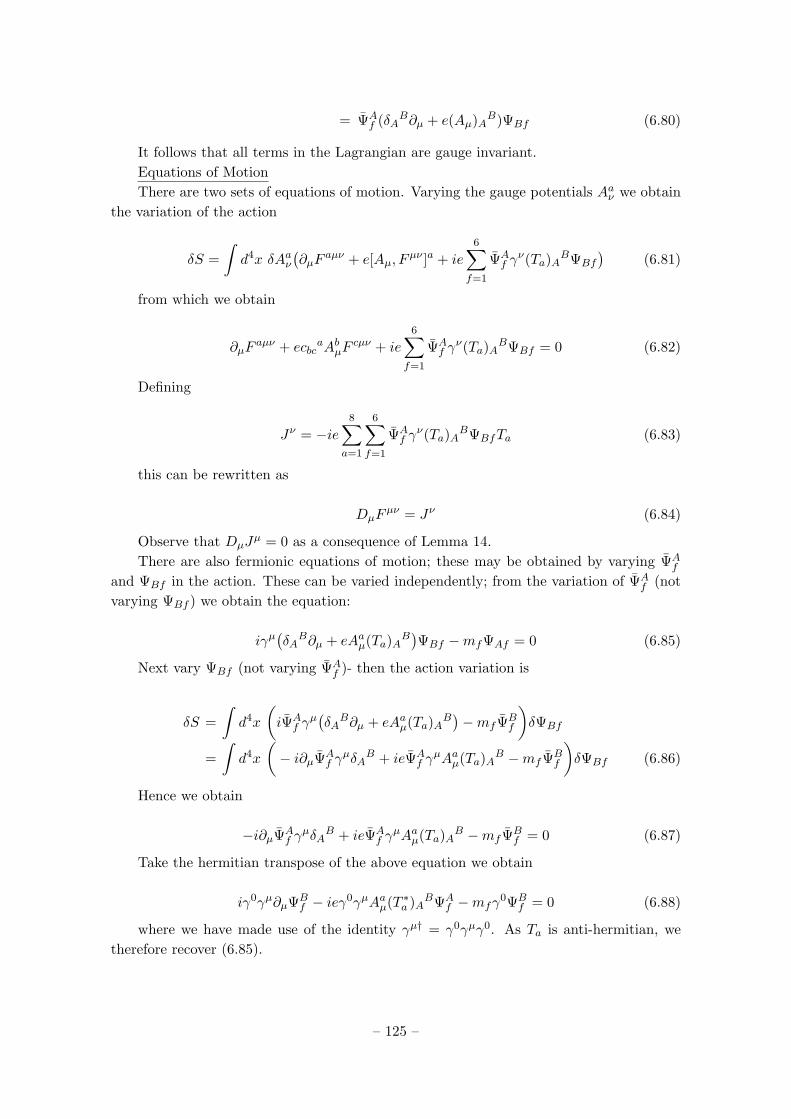
= ΨAf (δAB∂µ + e(Aµ)AB)ΨBf (6.80)

It follows that all terms in the Lagrangian are gauge invariant.Equations of MotionThere are two sets of equations of motion. Varying the gauge potentials Aaν we obtain

the variation of the action

δS =∫d4x δAaν

(∂µF

aµν + e[Aµ, Fµν ]a + ie

6∑f=1

ΨAf γ

ν(Ta)ABΨBf

)(6.81)

from which we obtain

∂µFaµν + ecbc

aAbµFcµν + ie

6∑f=1

ΨAf γ

ν(Ta)ABΨBf = 0 (6.82)

Defining

Jν = −ie8∑

a=1

6∑f=1

ΨAf γ

ν(Ta)ABΨBfTa (6.83)

this can be rewritten as

DµFµν = Jν (6.84)

Observe that DµJµ = 0 as a consequence of Lemma 14.

There are also fermionic equations of motion; these may be obtained by varying ΨAf

and ΨBf in the action. These can be varied independently; from the variation of ΨAf (not

varying ΨBf ) we obtain the equation:

iγµ(δA

B∂µ + eAaµ(Ta)AB)ΨBf −mfΨAf = 0 (6.85)

Next vary ΨBf (not varying ΨAf )- then the action variation is

δS =∫d4x

(iΨA

f γµ(δA

B∂µ + eAaµ(Ta)AB)−mf ΨB

f

)δΨBf

=∫d4x

(− i∂µΨA

f γµδA

B + ieΨAf γ

µAaµ(Ta)AB −mf ΨBf

)δΨBf (6.86)

Hence we obtain

−i∂µΨAf γ

µδAB + ieΨA

f γµAaµ(Ta)AB −mf ΨB

f = 0 (6.87)

Take the hermitian transpose of the above equation we obtain

iγ0γµ∂µΨBf − ieγ0γµAaµ(T ∗a )ABΨA

f −mfγ0ΨB

f = 0 (6.88)

where we have made use of the identity 㵆 = γ0γµγ0. As Ta is anti-hermitian, wetherefore recover (6.85).

– 125 –