SYMMETRIES IN THE OPTIMAL CONTROL OF SOLAR SAIL SPACECRAFTcdhall/papers/SolarSail.pdf · SYMMETRIES IN THE OPTIMAL CONTROL OF SOLAR SAIL SPACECRAFT M. KIM and C. D. HALL Department

SYMMETRIES IN THE OPTIMAL CONTROL OF SOLAR SAILSPACECRAFT

M. KIM and C. D. HALLDepartment of Aerospace and Ocean Engineering

Virginia Polytechnic Institute and State UniversityBlacksburg, Virginia 24061, USA

e–mails: [email protected], [email protected]

Abstract. The theory of optimal control is applied to obtain minimum–time trajectories for solarsail spacecraft for interplanetary missions. We consider the gravitational and solar radiation forcesdue to the Sun. The spacecraft is modelled as a flat sail of mass m and surface area A and is treateddynamically as a point mass. Coplanar circular orbits are assumed for the planets. We obtainoptimal trajectories for several interrelated problem families and develop symmetry properties thatcan be used to simplify the solution–finding process. For the minimum–time planet rendezvousproblem we identify different solution branches resulting in multiple solutions to the associatedboundary value problem. We solve the optimal control problem via an indirect method using anefficient cascaded computational scheme. The global optimizer uses a technique called AdaptiveSimulated Annealing. Newton and Quasi–Newton Methods perform the terminal fine tuning of theoptimization parameters.

Key words: Solar sail, Optimal control, Interplanetary missions, Symmetry.

1. Introduction

The concept of using solar radiation pressure as a means of propulsion for space vehicleswas first introduced in the 1920s by Tsiolkovsky (1921) and Tsander (1967 (quoting a 1924report by the author)). About fifty years later, the effect of solar radiation on spacecraftattitude dynamics was first experienced with the Mariner 10 mission to Mercury and Venus.Mariner 10 was also the first spacecraft to use a gravity assist trajectory, accelerating as itentered the gravitational influence of Venus, then using the planet’s gravity field to moveonto a slightly different course to reach Mercury. Since then, there have been severalattempts to realize a solar sail mission. In his book Wright (1992) presents a detailedanalysis on some possible solar sail applications. During his time at the Jet PropulsionLaboratory (JPL) Wright was actively involved in the planning of a rendezvous mission tocomet Halley using solar sail technology. In 1977 a solar electric propulsion concept wasselected instead, primarily because of technology maturity. Not long thereafter, the Halleyrendezvous mission was dropped by NASA.

During the development of the solar sail spaceflight concept, numerous studies of the

1

2 M. KIM and C. D. HALL

associated dynamics problem were presented. The first solar sail trajectories were calculatedby Tsu (1959) and London (1960). Tsu investigated various means of propulsion and showedthat in many cases solar sails show superior performance when compared to chemical andion propulsion systems. The author used approximated heliocentric motion equations toobtain spiraling trajectories for a “. . .fixed sail setting”. London presented similar spiralsolutions for Earth–Mars transfers with constant sail orientation using the exact equations ofmotion. Optimal solar sail trajectories were first computed by Zhukov and Lebedev (1964)for interplanetary missions between coplanar circular orbits. In 1980 Jayaraman (1980)published similar minimum–time trajectories for transfers between the Earth and Mars.Two years later, Wood et al. (1982) presented an analytical proof to show that the orbitaltransfer times obtained by Jayaraman (1980) were incorrect due to the incorrect applicationof a transversality condition of variational calculus and an erroneous control law. Powerset al. (1999) and Powers and Coverstone (2001) obtained results similar to those reportedin Wood’s paper, and obtained solutions for transfers to synchronous orbits. The moregeneral time–optimal control problem of three–dimensional, inclined and elliptic departureand rendezvous planet orbits was discussed by Sauer (1976). Hughes and McInnes (2001)used Genetic Algorithms and Sequential Quadratic Programming to obtain interplanetarytrajectories via a direct method. In a recent paper Dachwald (2004) presented a novelapproach based on Evolutionary Neurocontrollers (ENC) to calculate optimal solar sailtrajectories for interplanetary missions.

The paper is organized as follows: In the following sections we introduce the systemmodel and the corresponding motion equations. Subsequently, we define the minimum–timeoptimal control problem and present various optimal control problem families. We discusssystem symmetries and show how these symmetries can be used to great advantage to findoptimal control solutions. We outline the numerical algorithm with focus on the globaloptimization algorithm, namely, Simulated Annealing (SA). Finally we present simulationresults for each of the optimal control problem families and discuss the relationship betweenthe various families.

2. System Model And Motion Equations

The system model is illustrated in Figure 1. The spacecraft is modelled as a perfectly flatsolar sail of mass m and surface area A and is treated dynamically as a point mass. Wedefine the body–fixed reference frame bx, by with the bx axis identifying the solar sailsurface normal vector. The sail orientation angle α is defined as the angle between the sailnormal (= bx) and the solar flux direction S. A positive angle rotates bx anti–clockwiseinto S. For convenience, we define S⊥ as the unit vector orthogonal to S such that S⊥and by are aligned for α = 0. The environmental forces acting on the spacecraft system aredue to the gravitational field and the radiation pressure of the Sun. The initial and targetspacecraft trajectories are modelled as heliocentric, circular, and coplanar orbits.

We define the generalized coordinate vector as r , (r, θ)T and the corresponding velocityvector as v , (vr, vθ)T , where vr = r and vθ = rθ. In the inertial reference frame the motion

OPTIMAL CONTROL OF SOLAR SAIL SPACECRAFT 3

equations for a perfectly reflective solar sail spacecraft are then (McInnes, 1999)

r = vr (1)θ = vθ/r (2)

vr = β cos3 α/r2 + v2θ/r − 1/r2 (3)

vθ = β sinα cos2 α/r2 − vrvθ/r (4)

where β is the nondimensional characteristic acceleration. The motion equations can berewritten in condensed form as x = f(x, u), where the state vector and control input aredefined as x = (r, θ, vr, vθ)T and u = α. Typical normalized boundary conditions for thesystem (1–4) are

r(t0) = r0 θ(t0) = free vr(t0) = 0 vθ(t0) = 1/√

r0 (5)r(tf ) = rf θ(tf ) = θf or free vr(tf ) = 0 vθ(tf ) = 1/

√rf (6)

Note that depending on the particular optimal control problem family the angular boundarycondition has to be chosen appropriately. For the minimum–time orbit transfer problem,θ(tf ) = free, whereas for the minimum–time planet rendezvous problem θ(tf ) = θf . There-fore, we choose as the end–point constraint for the general minimum–time optimal controlproblem

ψ (x(tf ), tf ) =(r(tf )− rf , θ(tf )− θf , vr(tf ), vθ(tf )− 1/

√rf

)T = 0 (7)

In the next section we formulate the optimal control problem.

3. Optimal Control Problem Formulation

The optimal control problem is to find an optimal control input u? for a generally nonlinearsystem x = f(x, u, t) such that the associated performance index

J = φ (x(tf ), tf ) +∫ tf

t0

L(x,u, t) dt (8)

is minimized, and such that the constraint at final time tf

ψ (x(tf ), tf ) = 0 (9)

is satisfied. In equations (8,9) x is the n–dimensional state vector, u is the m–dimensionalcontrol input, and φ and L are the terminal and accumulated costs, respectively. Insteadof solving a constrained optimization problem, it is usually advantageous to consider thecorresponding unconstrained optimization problem using the augmented performance index

J + = φ (x(tf ), tf ) + νT ψ (x(tf ), tf ) +∫ tf

t0

L(x, u, t) + λT (f(x, u, t)− x)

dt (10)

Defining the Hamiltonian function H as

H = L(x, u, t) + λT f(x,u, t) (11)


the state and costate equations are obtained as

x =∂H∂λ

= f(x, u, t) and λ = −∂H∂x

= −∂L(x, u, t)∂x

− ∂f(x, u, t)∂x

λ (12)

Equations (12), combined with a set of appropriate boundary conditions for the states andcostates, yield a well–defined Boundary Value Problem (BVP). By specifying sets of end–and (where necessary) interior–point constraints, various control problem families can beidentified:

P0 . Minimum–time transfer between an initial and a target orbit. There is no angularend–point constraint; that is θ(tf ) = free.

P1 . P0 transfer with subsequent P0 return transfer to initial orbit. There are no angularinterior– and end–point constraints; that is, θ(ti) = free and θ(tf ) = free.

P2 . Minimum–time rendezvous with a target planet. The angular end–point constraintdepends on the initial angular separation between initial and target planet, and thesynodic period of the target planet; that is θ(tf ) = θf .

P3 . Minimum–time transfer including a target planet rendezvous and subsequent returnto initial planet. The angular constraints are θ(ti) = θi and θ(tf ) = θf .

In the following we present the optimality conditions and discuss specifics of each of thecontrol problem families introduced above.

3.1. Optimality conditions

For the general minimum–time transfer problem using the Lagrange formulation, the Hamil-tonian is given by

H = λ1vr + λ2vθ/r + λ3

(β cos3 α/r2 + v2

θ/r − 1/r2)

+ λ4

(β sinα cos2 α/r2 − vrvθ/r

)(13)

The corresponding costate equations are defined by λ = −∂H/∂x and are given as

λ1 = λ2vθ/r2 + (14)λ3

(2β cos3 α/r3 + v2

θ/r2 − 2/r3)

+ λ4

(2β sinα cos2 α/r3 − vrvθ/r2

)

λ2 = const.

= 0 iff θ(tf ) = free6= 0 iff θ(tf ) = θf

(15)

λ3 = −λ1 + λ4vθ/r (16)λ4 = −λ2/r − 2λ3vθ/r + λ4vr/r (17)

Applying Pontryagin’s Minimum Principle (Bryson and Ho, 1975), the optimal controlu? ≡ α? is chosen such that the Hamiltonian H is minimized; that is,

u? = arg minu∈U

H (x?, λ?, u) , ∀t > 0 (18)


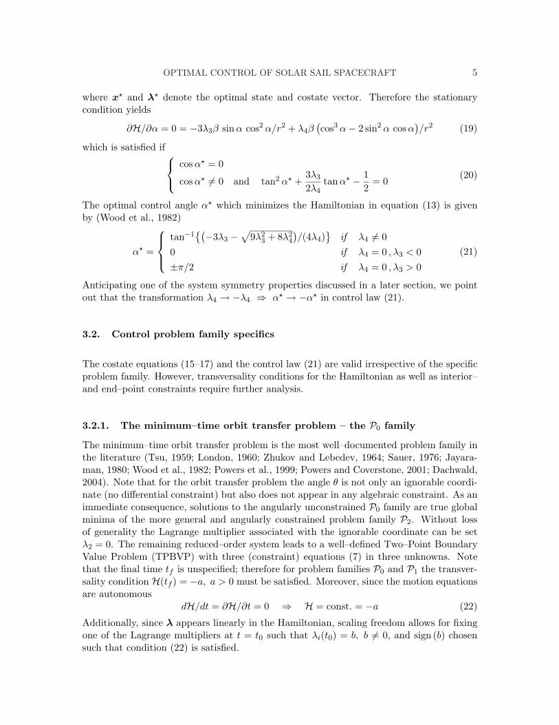
where x? and λ? denote the optimal state and costate vector. Therefore the stationarycondition yields

∂H/∂α = 0 = −3λ3β sinα cos2 α/r2 + λ4β(cos3 α− 2 sin2 α cosα

)/r2 (19)

which is satisfied if

cosα? = 0

cosα? 6= 0 and tan2 α? +3λ3

2λ4tanα? − 1

2= 0

(20)

The optimal control angle α? which minimizes the Hamiltonian in equation (13) is givenby (Wood et al., 1982)

α? =

tan−1(−3λ3 −

√9λ2

3 + 8λ24

)/(4λ4)

if λ4 6= 0

0 if λ4 = 0 , λ3 < 0±π/2 if λ4 = 0 , λ3 > 0

(21)

Anticipating one of the system symmetry properties discussed in a later section, we pointout that the transformation λ4 → −λ4 ⇒ α? → −α? in control law (21).

3.2. Control problem family specifics

The costate equations (15–17) and the control law (21) are valid irrespective of the specificproblem family. However, transversality conditions for the Hamiltonian as well as interior–and end–point constraints require further analysis.

3.2.1. The minimum–time orbit transfer problem – the P0 family

The minimum–time orbit transfer problem is the most well–documented problem family inthe literature (Tsu, 1959; London, 1960; Zhukov and Lebedev, 1964; Sauer, 1976; Jayara-man, 1980; Wood et al., 1982; Powers et al., 1999; Powers and Coverstone, 2001; Dachwald,2004). Note that for the orbit transfer problem the angle θ is not only an ignorable coordi-nate (no differential constraint) but also does not appear in any algebraic constraint. As animmediate consequence, solutions to the angularly unconstrained P0 family are true globalminima of the more general and angularly constrained problem family P2. Without lossof generality the Lagrange multiplier associated with the ignorable coordinate can be setλ2 = 0. The remaining reduced–order system leads to a well–defined Two–Point BoundaryValue Problem (TPBVP) with three (constraint) equations (7) in three unknowns. Notethat the final time tf is unspecified; therefore for problem families P0 and P1 the transver-sality condition H(tf ) = −a, a > 0 must be satisfied. Moreover, since the motion equationsare autonomous

dH/dt = ∂H/∂t = 0 ⇒ H = const. = −a (22)

Additionally, since λ appears linearly in the Hamiltonian, scaling freedom allows for fixingone of the Lagrange multipliers at t = t0 such that λi(t0) = b, b 6= 0, and sign (b) chosensuch that condition (22) is satisfied.


3.2.2. The minimum–time two–way orbit transfer problem – the P1 family

Minimum–time two–way orbit transfer problems present a challenging extension to the P0

family in that additional interior–point constraints have to be satisfied. One approach tosolve the resulting Three–Point Boundary Value Problems is to convert the problem to anequivalent TPBVP. By doing so, the interior point and boundary points of the Three–PointBoundary Value Problem are transformed to initial and final points of the TPBVP. Theresulting TPBVP is of higher dimension but less challenging to solve numerically. We solvethe Three–Point Boundary Value Problem following the procedure outlined in Bryson andHo (1975). At the interior point t0 < ti < tf boundary conditions of the form

υ(xi, ti) = (r(ti)− ri, vr(ti), vθ(ti)− 1/√

ri)T = 0 (23)

have to be satisfied. The corresponding jump conditions for the Lagrange multipliers thenyield

λr(t−i ) = λr(t+i ) + πT ∂υ

∂x(ti)= λr(t+i ) + π (24)

H(t−i ) = H(t+i )− πT ∂υ

∂ti= H(t+i ) (25)

where λr = (λ1, λ3, λ4)T are the Lagrange multipliers for the reduced system (λ2 = 0), πare the (constant) adjoined multipliers, and t−i and t+i signify the immediate points in timebefore and after t = ti, respectively. The increased complexity in solving for solutions of theP1 problem family stems from the additional unknowns: the adjoined multipliers π and theoptimal return transfer time. Note that a particular P1 solution can always be separatedinto two independent P0–type solutions due to missing angular constraints. Additionally,system symmetry can be used to great advantage to obtain one of the P0–type solutionsgiven the other. Symmetry properties are discussed in the following section.

3.2.3. The minimum–time planet rendezvous problem – the P2 family

For the rendezvous problem, the motion of the corresponding planets has to be taken intoaccount. The angular end–point constraint in equation (7) yields

θ(tf )− θf = 0 , where θf = T Θt −∆Θ(t0) = Tv3t −∆Θ(t0) (26)

In equation (26), T = tf − t0 is the transfer time, Θt and vt are angular rate and velocityof the target planet, and ∆Θ(t0) is the initial angular separation between initial and targetplanet. Note that due to system symmetry

∆Θ(t0) = −sign(Θi − Θt

)(Θi(t0)−Θt(t0)) ; (27)

that is, ∆Θ(t0) in equation (26) only depends on the relative orientation of initial andtarget planet. Also, with constraint (26) the transversality condition for the Hamiltonianfor problem families P2 and P3 becomes H(tf ) = H = a, a indefinite (as opposed toH(tf ) = −a, a > 0 for the angularly unconstrained P0 and P1 families). As before, withscaling freedom, λi(t0) = b, b 6= 0 and sign

(b)

chosen to satisfy H = a.


3.2.4. The minimum–time two–way planet rendezvous problem – the P3

family

Unlike for the P1 problem family we conjecture that P3 transfers can not be separated intotwo independent P2–type solutions. As mentioned before, the standard approach to obtaintwo–way trajectories is to solve the associated Three–Point Boundary Value Problems withappropriately chosen interior– and end–point constraints.

In the following section we discuss system symmetries as a means to assist in computingoptimal trajectories.

4. Symmetries

In the following we present and prove two system symmetries summarized in Theorem 1 andTheorem 2. Theorem 1 provides an effective tool to determine optimal return trajectories,which can be used to compute solutions of the P1 family efficiently. As pointed out inSection 3.2.2, solving the associated Three–Point Boundary Value Problem is not onlynumerically challenging but also a time–consuming process. Another interesting symmetryproperty is formulated in Theorem 2. Using nondimensional analysis one can show similarityof minimum–time solutions for the case when r(tf )/r(t0) = const. Moreover, there exists asimple relationship between transfer times and initial (or final) orbit radii for trajectorieswith r(tf )/r(t0) = const.

Definition A function Ω = (X,Λ, U, T )T is called a solution trajectory of the optimalcontrol problem if X and Λ are compatible solutions to the state equations (1–4) andcostate equations (15–17), respectively, with control history U and transfer time T , for agiven set of boundary values.

Theorem 1. Let Ω be a P0 solution trajectory satisfying the boundary conditions X(t0) =X0, X(tf ) = Xf , Λ(t0) = Λ0, and Λ(tf ) = Λf , then the costate solution for the corre-sponding return trajectory Ω∗ = (X∗,Λ∗, U∗, T ∗)T satisfies

Λ∗1(t∗) = −Λ1(t) , Λ∗2(t

∗) = Λ2(t) = 0 , Λ∗3(t∗) = Λ3(t) , Λ∗4(t

∗) = −Λ4(t) ,

witht∗ = T − t

and where T = tf − t0 = t∗f − t∗0 = T ∗.

Proof. The boundary conditions for the states are trivially compatible under the symmetrytransformation for the independent variable t. With (d/dt∗) = −(d/dt) it follows fromequation (1) that v∗r (t∗) = −vr(t) and from equation (3) that r∗(t∗) = r(t). For systeminvariance the control angle satisfies α∗(t∗) = −α(t) [equation (4)], which is compatiblewith the symmetry transformations for the Lagrange multipliers and the control law (21).Similarly, with the proposed symmetry transformations the costate equations are renderedinvariant.


Remark. Obviously, (−Λ1(tf ), Λ3(tf ),−Λ4(tf )) 7→ (Λ∗1(t∗0), Λ

∗3(t

∗0), Λ

∗4(t

∗0)) and the return

trajectory is readily propagated forward in time. For P0 solution trajectories θ is an ignor-able coordinate and does not appear in any algebraic constraints; therefore, Λ2 = Λ∗2 = 0without loss of generality.

Theorem 2. Let Ω be a P0 solution trajectory with Γ , r(tf )/r(t0) then the equivalent P0

solution trajectory Ω∗ with Γ∗ = Γ and r∗(t∗0) 6= r(t0) satisfies

X∗1 (t∗) = ξX1(t) , X∗

2 (t∗) = X2(t) , X∗3 (t∗) = ξ−1/2X3(t) , X∗

4 (t∗) = ξ−1/2X4(t) ,

Λ∗1(t∗) = ξ−3/2Λ1(t) , Λ∗2(t

∗) = Λ2(t) = 0 , Λ∗3(t∗) = Λ3(t) , Λ∗4(t

∗) = Λ4(t) ,

witht∗ = σt and therefore T ∗/ T = σ ≡ ξ3/2

where ξ = r∗(t∗0)/r(t0) = r∗(t∗f )/r(tf ) , T = tf − t0 , and T ∗ = t∗f − t∗0 .

Proof. Using as reference distance units 1 DU = r(t0) and 1 DU∗ = r∗(t∗0) to nondimen-sionalize motion equations and to obtain the corresponding solution trajectories Ω and Ω∗

the state and costate transformations render the systems of differential equations equivalentprovided that

µ TU 2/DU 3 = µ TU∗ 2/DU∗ 3

Remark. For solution trajectories that are not readily obtained with Theorem 1 and Theo-rem 2, for example, Γ∗ 6= Γ and r∗0 6= r0, Theorem 2 can be used to reduce the two–parametercontinuation problem to a one–parameter continuation problem as follows:

1. Compute Ω with Γ = Γ, r0 = r∗0 (or rf = r∗f ), using Theorem 2

2. Use homotopy to calculate Ω∗ with r∗0 = r0 (or r∗f = rf ) fixed

Also note the similarity between Kepler’s Third Law and the equation in Theorem 2 de-scribing the relationship between minimum transfer times and corresponding initial (orequivalently final) radial distances.

5. Numerical Approach

The inherent difficulty of global optimization problems lies in finding the best optimum froma possible multitude of local optima. In using indirect methods to solve optimum controlproblems, the difficulty stems from the fact that the initial conditions of the Lagrange mul-tipliers of the associated TPBVP cannot be estimated – not even approximately – withoutextensive analysis. von Stryk and Bulirsch (1992) and later Seywald and Kumar (1996)introduced the idea of combining direct and indirect methods to obtain approximate solu-tions with the direct method and to generate accurate solutions with the indirect method.An obvious drawback of this approach is that by using two fundamentally different solutionmethodologies, the control problem must be formulated twice, as well. Also, an interfaceis necessary to communicate between the two algorithms (Lagrange multipliers). In thispaper the optimization problem is solved with a cascaded computational scheme using anindirect method.


5.1. The computational scheme

Figure 2 illustrates the computational scheme. The qualitative performance of each of thethree methods used is indicated in the left part of the figure, with one star indicating rela-tively poor performance, and three stars indicating relatively good performance. SimulatedAnnealing (SA) is a global, statistical optimization algorithm, which was first introducedby Kirkpatrick et al. (1983) to solve discrete optimization problems such as computer chippacking and wiring, and to analyze classical problems such as the travelling salesman prob-lem (Cerny, 1985). We use a variant of the SA algorithm, namely Adaptive SimulatedAnnealing (Ingber and Rosen, 1992), as the initial optimization tool to obtain approximateestimates for the costates and the optimal transfer time T = tf − t0. Since statistical algo-rithms are in general neither efficient nor accurate, the global algorithm is used to identifythe region in the parameter space that contains the true global minimum.

Once the algorithm has located a set of parameters in close vicinity of the optimalset, a Quasi–Newton method (Gill et al., 1999) is used to further refine the parameter set.A crucial aspect of Quasi–Newton methods is the computation of second–order derivativeinformation. Rather than calculating the Hessian of the objective function accurately atevery iteration step or even just every so often we found that approximate Hessian informa-tion obtained using update formulas can significantly increase the algorithm effectiveness.In particular the Inverse Rank–One update (Gill et al., 1999) and the Inverse–Broyden–Fletcher–Goldfarb–Shanno (IBFGS) update (Gill et al., 1999) provide satisfactory opti-mization performance.

Newton’s method is known to be the most efficient zero–finding algorithm provided thestarting guess of the unknowns lies within the region of attraction of the algorithm. Used incombination with a Quasi–Newton method Newton’s method presents an efficient approachto obtain accurate solutions for the present problem.

5.2. Simulated annealing – A global, statistical optimization algorithm

The term simulated annealing (SA) derives from the analogous physical process of thermalannealing (metallurgy) to obtain a defect–free (and so in some sense optimized) crystallinestructure. In an annealing process a melt, initially at high temperature and disordered, iscooled in a controlled, slow manner to keep the system in an approximate state of thermo-dynamic equilibrium (adiabatic cooling). As cooling proceeds, the system becomes orderedand approaches a ground state. In a SA optimization algorithm, the annealed substancecorresponds to the system being optimized. Similarly, the current “energy” state of thesubstance corresponds to the current value of the system cost function, with the goal ofidentifying the ground state of the system, the global minimum. The internal microscopicinteractions that keep the substance in a state of thermodynamical equilibrium are simu-lated in SA by a sequence of parameter perturbations described by Markov chains. Onemajor difficulty of implementing a SA algorithm is that there is no obvious analog to the


temperature in the physical process. The corresponding SA control parameter serves as areference energy defining the boundary between the local and global vicinity of the currentoptimal parameter set in parameter space.

In general statistical optimization methods such as Simulated Annealing differ fromdeterministic techniques in that the iteration procedure need not converge towards a localoptimum since transitions thereout are always possible. Another feature is that an adaptivedivide–and–conquer occurs: coarse features of the optimal parameter set appear at highertemperatures, fine details develop at lower temperatures. For a detailed analysis on SA werefer to Kirkpatrick et al. (1983), Cerny (1985), and Ingber and Rosen (1992).

6. Simulation Results

Results obtained for Earth–Mars P0 transfers are in excellent agreement with data pub-lished by Wood et al. (1982). Table I shows transfer times and initial and final costatesfor two different characteristic accelerations. We obtained high–accuracy results with|ψ (x(tf ), tf ) | < 10−14, which result in slightly improved transfer times in the order of 10 to15 hours compared to reported results in Wood et al. (1982). Note that the nondimensionalcharacteristic accelerations of β = 0.16892 and β = 0.33784 correspond to nominal valuesof β = 1 mm/s2 and β = 2 mm/s2. The minimum transfer times correspond to 323.87 and407.62 days, respectively (1 TU = 365.25/(2π) days = 58.1313 days).

Figure 3 shows minimum transfer time versus target orbit radius for P0 orbit transfersstarting at 1 AU and for three different characteristic accelerations. According to McInnes(1999), state–of–the–art solar sail spacecraft achieve reasonable characteristic accelerationson the order of β / 2 mm/s2; thus β = 3.3784 is only of pedagogical value. Note theincreased “sail effectiveness” due to the 1/r2 potential field for inbound trajectories whencompared to outbound trajectories; that is, inbound transfers take comparatively less timethan outbound transfers.

Symmetry properties discussed in Section 4 are illustrated in Figures 4 and 5 and Ta-ble II. Figure 4 shows two outbound trajectories, Ω1 and Ω2, with Γ1 = Γ2 = 2, andr1(t1 = 0) = 1 AU and r2(t2 = 0) = 1.5 AU, respectively, and one inbound trajectory,Ω3, with Γ3 = 1/2 and r3(t3 = 0) = 1.5 AU. As shown in Theorem 2, α1(t1) = α2(t2) orequivalently, α1(τ) = α2(τ) on the unit time interval with τ ∈ [0, 1]. Also, for the outboundtrajectories σ = 1.8371 = 1.53/2 with T2 = 16.6176 and T1 = 9.0455. Using both Theoremsthe inbound trajectory satisfies α2(t2) = −α3(t3). The inbound transfer time results areT3 = 5.8752 and σ = T2/ T3 = 23/2, as expected. As pointed out in Section 3.2.2, P1 solutiontrajectories can be obtained by either solving the associated Three–Point Boundary ValueProblem or by solving for the corresponding P0 solution and using Theorem 1. Figure 5shows a P1 Earth–Mars–Earth transfer for β = 0.33784 obtained by solving the Three–PointBoundary Value Problem. Similarly to Figure 4 the sail orientation angle clearly shows sys-tem symmetry. Accompanying simulation data are listed in Table II. Note that the initial,and therefore also the final, Lagrange multipliers are scaled such that λ1(t0) = −1 and


λ1(tf ) = +1. The adjoined multipliers π, are essential to solve the boundary value problem(BVP), but dispensable when using symmetry (dashed–lined arrows).

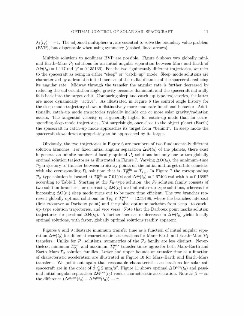
Multiple solutions to nonlinear BVP are possible. Figure 6 shows two globally mini-mal Earth–Mars P2 solutions for an initial angular separation between Mars and Earth of∆Θ(t0) = 1.117 rad (β = 0.135136). For the two significantly different trajectories, we referto the spacecraft as being in either “sleep” or “catch–up” mode. Sleep–mode solutions arecharacterized by a dramatic initial increase of the radial distance of the spacecraft reducingits angular rate. Midway through the transfer the angular rate is further decreased byreducing the sail orientation angle, gravity becomes dominant, and the spacecraft naturallyfalls back into the target orbit. Comparing sleep and catch–up type trajectories, the latterare more dynamically “active”. As illustrated in Figure 6 the control angle history forthe sleep mode trajectory shows a distinctively more moderate functional behavior. Addi-tionally, catch–up mode trajectories typically include one or more solar gravity/radiationassists. The tangential velocity vθ is generally higher for catch–up mode than for corre-sponding sleep mode trajectories. Not surprisingly, once close to the object planet (Earth)the spacecraft in catch–up mode approaches its target from “behind”. In sleep mode thespacecraft slows down appropriately to be approached by its target.

Obviously, the two trajectories in Figure 6 are members of two fundamentally differentsolution branches. For fixed initial angular separation ∆Θ(t0) of the planets, there existin general an infinite number of locally optimal P2 solutions but only one or two globallyoptimal solution trajectories as illustrated in Figure 7. Varying ∆Θ(t0), the minimum–timeP2 trajectory to transfer between arbitrary points on the initial and target orbits coincideswith the corresponding P0 solution; that is, Tmin

P2= TP0 . In Figure 7 the corresponding

P0–type solution is located at TminP2

= 7.01204 and ∆Θ(t0) = 2.67402 rad with β = 0.16892according to Table I. Starting at the P0–type solution, the P2 solution family consists oftwo solution branches: for decreasing ∆Θ(t0) we find catch–up type solutions, whereas forincreasing ∆Θ(t0) sleep mode turns out to be more time–efficient. The two branches rep-resent globally optimal solutions for TP2 6 Tmax

P2= 12.59186, where the branches intersect

(first crossover = Darboux point) and the global optimum switches from sleep– to catch–up–type solution trajectories, and vice versa. Note that the Darboux point marks solutiontrajectories for pessimal ∆Θ(t0). A further increase or decrease in ∆Θ(t0) yields locallyoptimal solutions, with faster, globally optimal solutions readily apparent.

Figures 8 and 9 illustrate minimum transfer time as a function of initial angular sepa-ration ∆Θ(t0) for different characteristic accelerations for Mars–Earth and Earth–Mars P2

transfers. Unlike for P0 solutions, symmetries of the P2 family are less distinct. Never-theless, minimum Tmin

P2and maximum Tmax

P2transfer times agree for both Mars–Earth and

Earth–Mars P2 solution families. Lower and upper bounds on transfer time as a functionof characteristic acceleration are illustrated in Figure 10 for Mars–Earth and Earth–Marstransfers. We point out again that reasonable characteristic accelerations for solar sailspacecraft are in the order of β / 2 mm/s2. Figure 11 shows optimal ∆Θopt(t0) and pessi-mal initial angular separation ∆Θpes(t0) versus characteristic acceleration. Note as β →∞the difference (∆Θopt(t0)−∆Θpes(t0)) → π.


7. Summary and Conclusions

We study the optimal control problem of solar sail spacecraft for planar interplanetarymissions in detail. The optimization problem is solved using an indirect method. Thecascaded computational scheme is divided into two optimization levels. On the first levela global statistical algorithm based on Adaptive Simulated Annealing is used to find anapproximate guess for the Lagrange multipliers and the transfer time. The optimizationparameters are then refined using a Quasi–Newton method. The final optimization stageis realized using a Newton’s method. The composite algorithm proves extremely efficientfinding highly accurate solutions to the minimum–time control problem.

We obtain optimal trajectories for several interrelated problem families that are de-scribed as Multi–Point Boundary Value Problems. We present and prove two theoremsdescribing system symmetries. We demonstrate how these symmetry properties can beused to significantly simplify the solution–finding process. For the minimum–time transferbetween two planetary orbits with subsequent return transfer, only a Two–Point Bound-ary Value Problem has to be solved when using symmetry as opposed to the associatedThree–Point Boundary Value Problem. Another system symmetry allows for efficient com-putation of solution trajectories by replacing a two–parameter continuation problem by acorresponding one–parameter continuation problem.

8. Future Work

In the future we intend to analyze more complex optimal control problems such as non–planar transfers between planets in elliptical orbits. From a dynamics point of view it isunlikely that symmetries exist for minimum–time transfer problems with arbitrary planetaryorbits. Nevertheless, the approach presented in this paper can be used to generate initialguesses for the costate vector for the more general class of optimization problems.

Choosing the solar sail orientation angle as the control variable yields analytically sim-ple control laws for spacecraft modelled as point masses. In practice, however, a rigid–body model might be more appropriate. Consequently, a combination of control forces andtorques replaces the solar sail orientation angle as the control variable. As an interestingconsequence, the particular choice of control variables might yield bang–type control lawswith the controls (forces and torques) appearing linearly in the Hamiltonian, which in turncould entail controllability issues.

Acknowledgements

The authors would like to thank Dr. Eugene Cliff for several fruitful discussions during thepreparation of this work.


References

Bryson, Jr. A. E. and Ho, Yu-Chi. 1975. Applied Optimal Control. Taylor & Francis.Revised Printing.

Cerny, V., 1985. Thermodynamical approach to the traveling salesman problem: An efficientsimulation algorithm. Journal of Optimization Theory and Applications, 45(1), 41–51.

Dachwald, B., 2004. Optimization of interplanetary solar sailcraft trajectories using evolu-tionary neurocontrol. Journal of Guidance, Control, and Dynamics, 27(1), 66–72.

Gill, P. E., Murray, W., and Wright, M. H. 1999. Practical Optimization. Academic PressLimited, 24/28 Oval Road, London NW1 7DX.

Hughes, G. W. and McInnes, C. R. 2001. Solar sail hybrid trajectory optimization. Proceed-ings of the 2001 AAS/AIAA Astrodynamics Specialist Conference, Quebec City, Quebec,Canada, volume 109 of Advances in the Astronautical Sciences, pages 2369–2380.

Ingber, L. and Rosen, B., 1992. Genetic algorithms and very fast simulated reannealing: Acomparison. Mathematical and Computer Modelling, 16(11), 87–100.

Jayaraman, T. S., 1980. Time–optimal orbit transfer trajectory for solar sail spacecraft.Journal of Guidance and Control, 3(6), 536–542.

Kirkpatrick, S., Gelatt, Jr., C. D., and Vecchi, M. P., 1983. Optimization by simulatedannealing. Science, 220(4598), 671–680.

London, H. S., 1960. Some exact solutions of the equations of motion of a solar sail withconstant sail setting. American Rocket Society Journal, 30, 198–200.

McInnes, C. R. 1999. Solar Sailing: Technology, Dynamics, and Mission Applications. SpaceScience and Technology. Springer. Published in association with Praxis Publishing.

Powers, R. B. and Coverstone, V. L., 2001. Optimal solar sail orbit transfers to synchronousorbits. The Journal of the Astronautical Sciences, 49(2), 269–281.

Powers, R. B., Coverstone-Carroll, V. L., and Prussing, J. E. 1999. Solar sail optimalorbit transfers to synchronous orbits. Proceedings of the 1999 AAS/AIAA AstrodynamicsSpecialist Conference, Girdwood, Alaska, volume 103 of Advances in the AstronauticalSciences, pages 523–538.

Sauer, C. G. 1976. Optimum solar–sail interplanetary trajectories. Paper presented atAIAA/AAS Astrodynamics Conference, San Diego, CA, AIAA Paper 76–792.

Seywald, H. and Kumar, R. R., 1996. Method for automatic costate calculation. Journalof Guidance, Control, and Dynamics, 19(6), 1252–1261.

Tsander, K., 1967 (quoting a 1924 report by the author). From a scientific heritage. NASATechnical Translation TTF–541.


Tsiolkovsky, K. E., 1921. Extension of man into outer space. Cf. Also K. E. Tsiolkovskiy,Symposium on Jet Propulsion, No. 2, United Scientific and Technical Presses (NIT), 1936(in Russian).

Tsu, T. C., 1959. Interplanetary travel by solar sail. American Rocket Society Journal, 29,422–427.

von Stryk, O. and Bulirsch, R., 1992. Direct and indirect methods for trajectory optimiza-tion. Annals of Operations Research, 37, 357–373.

Wood, L. J., Bauer, T. P., and Zondervan, K. P., 1982. Comment on time–optimal orbittransfer trajectory for solar sail spacecraft. Journal of Guidance, Control, and Dynamics,5(2), 221–224.

Wright, J. L. 1992. Space Sailing. Gordon and Breach Science Publishers. Second printing1993.

Zhukov, A. N. and Lebedev, V. N., 1964. Variational problem of transfer between heliocen-tric orbits by means of a solar sail. Kosmicheskie Issledovaniya (Cosmic Research), 2,45–50.


Table IMinimum transfer times and corresponding costates for Earth–Mars transfers.

Analysis Characteristic Transfer time Initial costates Final costates

Wood et al. (1982)

Kim and Hall

Analysis Transfer time Initial costates Final costates

accelerationAuthors β T λr(0) λr(T )

0.16892 7.02232

−7.40981−4.22855−7.91115

−21.5481+ 8.5025−46.6174

0.33784 5.57911

−3.68044−2.59597−2.56421

−14.9271+10.1662−29.6344

0.16892 7.01204

−7.41099−4.23234−7.90591

−21.5482+ 8.5063−46.5737

0.33784 5.57134

−3.68301−2.59741−2.56208

−14.9274+10.1619−29.6045

Table IILagrange and adjoined multipliers for an Earth–Mars–Earth minimum–time transfer for

β = 0.33784.

Solution arc Earth orbit Mars orbit Transfer time

Outboundtrajectory

−1.00000−0.70524−0.69565

→

−4.05305+2.75912−8.03812

5.57134

Turningpoint

− 8.10610− 0.00000−16.07625

Inboundtrajectory

+1.00000−0.70524+0.69565

→

+4.05305+2.75912+8.03812

5.57134

Solution arc Lagrange multipliers λr(t) at Adjoined multipliers π Transfer time


Figure Captions

Figure 1: System model.

Figure 2: Cascaded numerical algorithm for solving the optimal control problem.

Figure 3: Transfer time as a function of target orbit radius. Initial orbit radius is 1 AU.

Figure 4: Minimum–time orbit transfer system symmetry.

Figure 5: Earth–Mars–Earth minimum–time orbit transfer for β = 0.33784.

Figure 6: Minimum–time Mars–Earth rendezvous trajectories for β = 0.135136.

Figure 7: Minimum transfer time for Mars–Earth rendezvous for β = 0.16892.

Figure 8: Minimum transfer time for Mars–Earth rendezvous.

Figure 9: Minimum transfer time for Earth–Mars rendezvous.

Figure 10: Minimum transfer time for optimal and pessimal initial phase difference betweenMars and Earth.

Figure 11: Optimal and pessimal initial phase difference between Mars and Earth versuscharacteristic acceleration.


ex,

eybx

by

r = (r, θ)T

α

α

m,A

S

Sail

Sun

Initial orbit/planet(circular, coplanar)

Target orbit/planet(circular, coplanar)

Solar flux

Figure 1. System model.


text

Newton Method

Quasi-Newton Method

Adaptive Simulated

Annealing

Stochastic

global

Deterministic

local

Conver

gence

radius

Conver

gence

rate

Accurac

y

δ1 6 ε1

δ2 6 ε2

Figure 2. Cascaded numerical algorithm for solving the optimal control problem.


0 0.25 0.5 0.75 10

5

10

15

20

25

30

Non

dim

ensi

onal

orb

it tr

ansf

er ti

me

1 1.25 1.5 1.75 2 2.25 2.5 2.75 3

Minimum orbit transfer time versus target orbit radius

Nondimensional target orbit radius

Mer

cury

Venu

s Mar

sβ = 0.16892 β = 0.33784β = 3.3784

➌

➋

➊

➌➋➊

➌

➋

➊

Figure 3. Transfer time as a function of target orbit radius. Initial orbit radius is 1 AU.


−3 −2 −1 0 1 2 3 −3

−2

−1

0

1

2

3

Transfer trajectories for β = 0.33784

Nondimensional x distance

Non

dim

ensi

onal

y d

ista

nce

0 0.2 0.4 0.6 0.8 1−90

−60

−30

0

30

60

90Solar sail orientation angle for β = 0.33784

Normalized time

Orie

ntat

ion

angl

e in

deg

1:2 outbound trajectories

2:1 inbound trajectory

0.75 AU

1.50 AU

Figure 4. Minimum–time orbit transfer system symmetry.


−1.5 −1 −0.5 0 0.5 1 1.5

−1.5

−1

−0.5

0

0.5

1

1.5

Transfer trajectory for β = 0.33784


Non

dim

ensi

onal

y d

ista

nce

0 2 4 6 8 10 12−90

−60

−30

0

30

60

90Solar sail orientation angle for β = 0.33784

Nondimensional time

Orie

ntat

ion

angl

e in

deg

T = 11.142 TU = 2 × 5.571 TU

Figure 5. Earth–Mars–Earth minimum–time orbit transfer for β = 0.33784.


−2 −1 0 1 2

−2

−1

0

1

2

Transfer trajectories for β = 0.135136


Non

dim

ensi

onal

y d

ista

nce

0 2 4 6 8 10 12 14−90

−60

−30

0

30

60

90Solar sail orientation angle for β = 0.135136 (0.8 mm/s2)

Nondimensional time

Orie

ntat

ion

angl

e in

deg

"catch"

"sleep"

"sleep"

"catch"

T = 13.975 TU, ∆Θ = 1.117 rad

Figure 6. Minimum–time Mars–Earth rendezvous trajectories for β = 0.135136.


−3 −2 −1 0 1 2 37

8

9

10

11

12

13

14

15

16

Initial phase difference ∆Θ between Mars and Earth

Non

dim

ensi

onal

tran

sfer

tim

e

Minimum transfer time for Mars−Earth rendezvous for β = 0.16892

Second crossover (local minimum)

First crossover = Darboux point (global minimum)

Catch−up mode

Catch−up mode

Sleep mode

"catch"

"sleep"

∆Θ = ∆Θpes

∆Θ = ∆Θopt

Figure 7. Minimum transfer time for Mars–Earth rendezvous for β = 0.16892.


−3 −2 −1 0 1 2 30

5

10

15

20

25

30

35

Initial phase difference ∆Θ between Mars and Earth

Non

dim

ensi

onal

tran

sfer

tim

e

Minimum transfer time for Mars−Earth rendezvous

First crossovers (global minima)

β = 3.3784 (20 mm/s2) T

min= 3.127 TU

β = 0.33784 (2 mm/s2) T

min= 5.571 TU

β = 0.16892 (1 mm/s2) T

min= 7.012 TU

β = 0.135136 (0.8 mm/s2) T

min= 7.625 TU

β = 0.101352 (0.6 mm/s2) T

min= 8.632 TU

β = 0.033784 (0.2 mm/s2) T

min= 23.965 TU

β = 0.050676 (0.3 mm/s2) T

min= 16.298 TU

β = 1.0000 (5.9 mm/s2) T

min= 4.118 TU

Figure 8. Minimum transfer time for Mars–Earth rendezvous.


−3 −2 −1 0 1 2 30

5

10

15

20

25

30

35

Initial phase difference between Mars and Earth

Non

dim

ensi

onal

tran

sfer

tim

e

Minimum transfer time for Earth−Mars rendezvous

First crossovers (global minima)

β = 0.033784 (0.2 mm/s2) T

min= 23.965 TU

β = 0.050676 (0.3 mm/s2) T

min= 16.298 TU

β = 0.101352 (0.6 mm/s2) T

min= 8.632 TU

β = 0.135136 (0.8 mm/s2) T

min= 7.625 TU

β = 0.16892 (1 mm/s2) T

min= 7.012 TU

β = 0.33784 (2 mm/s2) T

min= 5.571 TU

β = 3.3784 (20 mm/s2) T

min= 3.127 TU

Figure 9. Minimum transfer time for Earth–Mars rendezvous.


0 0.5 1 1.5 2 2.5 3 3.50

5

10

15

20

25

30

35

Nondimensional characteristic acceleration

Non

dim

ensi

onal

tran

sfer

tim

e

Minimum transfer time versus characteristicacceleration for Earth−Mars and Mars−Earth rendezvous

β = 0.2 mm/s2

β = 1.0 mm/s2

β = 2.0 mm/s2

β = 20.0 mm/s2

Minimum transfer time for optimal initial phase difference ∆Θ ~

~

~

~ β = 0.8 mm/s2 ~

β = 0.6 mm/s2 ~

Minimum transfer time for pessimal initial phase difference ∆Θ

β = 0.3 mm/s2 ~

Figure 10. Minimum transfer time for optimal and pessimal initial phase difference betweenMars and Earth.


0 0.5 1 1.5 2 2.5 3 3.5−1

0

1

2

3

4

5

6

7

8

9

Nondimensional characteristic acceleration

Initi

al p

hase

diff

eren

ce b

etw

een

Mar

s an

d E

arth

in r

ad

Initial phase difference for minimum time transfers between Marsand Earth versus characteristic acceleration for Mars−Earth rendezvous

β = 0.2 mm/s2 ~

~ β = 1.0 mm/s2

β = 2.0 mm/s2 ~

~ β = 20.0 mm/s2

β = 0.8 mm/s2

~ β = 0.6 mm/s2 ~

Optimal initial phase difference ∆Θfor minimum time transfer

Pessimal initial phase difference ∆Θfor minimum time transfer

β = 0.3 mm/s2 ~

Figure 11. Optimal and pessimal initial phase difference between Mars and Earth versuscharacteristic acceleration.

Documents

SYMMETRIES IN THE OPTIMAL CONTROL OF SOLAR SAIL SPACECRAFTcdhall/papers/SolarSail.pdf · SYMMETRIES IN THE OPTIMAL CONTROL OF SOLAR SAIL SPACECRAFT M. KIM and C. D. HALL Department