Symmetrical Linear Antennas Driven by Two-Wire Lines

SERBIAN JOURNAL OF ELECTRICAL ENGINEERING Vol. 1, No. 1, November 2003, 27 - 60

27

Symmetrical Linear Antennas Driven by Two-Wire Lines

Jovan V. Surutka1, Dragutin M. Veli~kovi 2

Abstract: A new theoretical approach to the problem of the symmetrical linear antenna driven by a two-wire line is presented. Then symmetrical linear antenna and the feeder line are treated as a unique boundary-value problem leading to a system of two simultaneous integral equations containing antenna and line cur-rents as unknown sub-integral functions. The integral equations are approxi-mately solved by the so-called point-matching method. Due to the mutual cou-pling between the antenna and the line, a new conveniently defined apparent driving-point admittance is to be introduced. The method is applied on several types of linear antennas: Centre driven symmetrical dipole antenna, Centre-driven V-antenna, Cage antenna, H-antenna and System of two parallel non-stag-gered dipoles antennas, positioned in the air over semi-conducting ground. Then theoretical results for admittances were compared with the experiments and re-markably good overall agreement has been found. On the contrary, a comparison with the corresponding theoretical results obtained with the idealized delta-func-tion generator revealed remarkable discrepancies.

Keywords: Linear antenna, Integral equation, Antenna input impedance, Two-wire line.

1 Introduction Many authors have exhaustively treated the problem of the thin symmetrical linear

antennas fed by a delta-function generator. Then moment method is commonly used for approximate numerical solving of existing integral equation, having antenna current distribution as unknown [1]. Especially, very good results in the numerical solving of these integral equations are obtained using point matching method with polynomial cur-rent distribution. First of all, polynomial current approximation was used in [2], for ap-proximate numerical solving of Hallen's integral equation [27]. Afterward, integral equa-tions and polynomial current approximation were successfully used for solving several types of linear antennas, as: Isolated [3] or Symmetrical dipole antenna in non-linear semi conducting media [4], V-dipole antenna [5] and Loop antenna [6, 7]. This tech-nique was later expanded on the curvilinear antennas [8] and on the linear antennas in the surroundings of conducting bodies [9]. Recently, very good results are obtained in

1 Serbian Academy des Sciences et des Arts, Belgrade, Serbia and Montenegro 2 Faculty of Electronic Engineering of Ni, Department of Electromagnetics, Beogradska 14, 18000 Ni,

Serbia and Montenegro, Phone: +381 18 529 429, Fax: +381 18 524 931, E-mail: [email protected]

J. V. Surutka, D. M. Veli~kovi

28

modelling cage structures in pulse external electromagnetic field (which imitate light-ning or nuclear explosion electromagnetic discharges) [10]. Except point matching method, polynomial antenna current approximation is successfully included in varia-tional solution of linear antenna problems, for solving V and Loop antennas [11-13].

If linear antennas are driven by delta-function generator, the comparison between theoretical and experimental results show very good agreement in determining of the antenna radiation pattern, near and far field distribution and antenna input conductance, but theoretical values of antenna input susceptance are always incorrect, because of the physical insufficiency of the delta-function generator. In order to exceed these difficul-ties, the authors suggest one new approach to solving linear symmetric antennas driven by two-wire lines. The first very good results are obtained in the analysis of symmetrical dipole [14] and V-antenna [15], including two non-staggered dipoles [16, 17, 18]. Af-terward, several more complex forms of linear antennas were treated in this way, as cage antenna [21], H-antenna [22], two arbitrary oriented symmetrical dipole antennas in free space [20] or near ground [19]. These investigations of the symmetrical linear antenna driven by a two-wire line have revealed a strong dependence of the input admittance on geometry of the feeding zone. Particularly remarkable discrepancies were noticed be-tween the theoretical admittances obtained with the delta function generator and those achieved with real feeding system comprising a two-wire line having the conventional distance between the line conductors.

In order to prove the theory, the theoretical results were compared with the experi-mental results obtained by Angelakos [23] and in the Antenna Laboratory of the Faculty of Electrical Engineering of Belgrade [24]. A very satisfactory overall agreement be-tween the results was found. On the other side, the comparison between of the theoreti-cal results of the present theory with those obtained by using an idealized delta-function generator shows remarkable discrepancies. Finally, it is not superfluous to notice the obtained results in very precise numerical solving of several types on non-elementary integrals having singular or quasi-singular sub-integral functions [25, 26], which eliminates eventual ill-condition problems in numerical solving of systems of simulta-neous integral equations.

2 Short Theoretical Approach The antenna and the line are treated as a unique boundary value problem, so that

the coupling between the antenna and the line, as well as the transmission line end effect are taken into account. Such a treatment leads to a system of two simultaneous integral equations, containing the current distributions on the antenna and on the line as terminal zone, in the vicinity of the antenna input terminals, as unknown subintegral functions. Due to the coupling between the antenna and the line, the line current can be represented as a simple sum of an incident and reflected travelling waves, as in the conventional transmission line theory. At that part of the line, an additional, perturbing term must be added to the travelling waves. As performed investigations shown, the length of this per-turbed part of the line is not critical and it may be satisfactorily taken to be between

λ0.1 and λ0.25 , where λ denotes the wavelength. These integral equations are solved numerically by using point-matching method. The current on the antenna is approxi-

Theory of Symmetrical Linear Antennas ...

29

mated by a polynomial with unknown complex coefficients and that on the line by the sum of an incident and reflected waves and by a polynomial decreasing rapidly with the distance from the end of the line. The concept of the input admittance of the antenna needs some clarifications and a new, adequate definition. Namely, due to the mutual coupling (by means of the field) between the antenna and the line, the usual definition of the admittance, as the ratio between the current and potential difference at the input ter-minals, is no longer a meaningful and useful concept. Much better and more suitable definition can be established when the antenna effects on the current and voltage distri-butions along the line beyond the terminal zone are taken into consideration. Since the conventional transmission line theory holds at that part of the line, the input admittance in any cross section of the line can be defined as the ratio of the current and the voltage in that section and can be expressed by means of the current reflection coefficient and characteristic admittance of the line. In order to define an "apparent driving-point admit-tance" of the antenna, the above-defined admittance is to be transformed to the end of the line according to the transmission line theory.

3 Description of the Method in the case of Symmetric centre-driven dipole antenna

3.1 The Apparent Admittance and Currents in the System Consider the circuit consisting of a balanced two-wire line terminated in a symmet-

ric centre-driven dipole antenna. The geometrical arrangement is shown in Fig.1. The dipole antenna consists of two straight, collinear cylindrical conductors, each of length h′ and small radius a , separated in the middle by a gap of half-length d . The distance from the centre of the dipole to each of its extremities is denoted by h , so dhh +′= .

The transmission line consists of two parallel conductors of radius b , the axes of which are separated by a distance d2 . The antenna and line conductors are assumed to be perfect.

As shown in Fig.1 the axis of the dipole coincides with the −z axis of the coordi-nate system, the −y axis of which is parallel to the axes of the two-wire line and bisects the distance between them.

In order to simplify the analysis it is assumed that the currents on the antenna and on the transmission line are localized on conductor axes. The positive directions of the currents are denoted on the Figure. Due to symmetry the current on the dipole arms,

( )zIa , must satisfy the condition

( ) ( )zIzI aa =− , dzh −≤≤− , hzd ≤≤ . (1)

In addition, the current ( )zIa must fulfil the condition

( ) 0=hIa . (2)


30

In writing the expression for the current on the transmission line, it is convenient to distinguish two parts of the line:

(1) The part Ly ≥ , where the direct influence of the dipole and of the end-discontinuity of the line can be neglected; and

(2) The part Ly <≤0 , where the coupling between the dipole and the line, as well as the line ends effect, must be taken into account.

Fig. 1 - Symmetric dipole antenna driven by a two-wire line.

As will be seen later, the choice of the length L is not critical. It is quite satisfac-tory to take it equal to a small multiple of the separation d2 between the line conduc-tors.

The current distribution function along the first part of the line, Ly ≥ , can be represented in a conventional manner as the sum of the incident and reflected waves,

( ) kyky IIyI jr

jif ee −−= , Ly ≥ , (3)

where iI and rI are unknown complex amplitudes of the two waves and

λπ2=µεω= 00k is the free space propagation constant.

To account for the influence of the dipole and of the line-end on the current distri-bution on the second part of the line, Ly ≤≤0 , an additional term ( )yIp should be

added to (3), so that

( ) ( )yIIIyI kykyp

jr

jif ee +−= − , Ly ≤≤0 . (4)


31

In order to preserve the continuity of the current at Ly = , the following condi-tions must be satisfied,

( ) 0=LIp and 0==Ly

yI dd p . (5)

In addition, the current at the end of the line must be equal to the current entering the dipole,

( ) ( )dII af 0 = . (6)

The form of equation (3) implies that on the part of the line Ly ≥ a TEM field exists, so that the conventional transmission-line theory is fully applicable. Conse-quently, the input admittance, ( )yY , in each cross-section of the part of the line Ly ≥ can be defined as

( ) ( ) ( ) ( ) RRY

IIZIIyVyIy ky

ky

kyky

kyky

+

−=

+

−==

−

−

2j

2j

cjr

jic

jr

ji

ffee

eeeeY , (7)

where cc 1 ZY = is the characteristic admittance of the line and

ir IIR = (8)

is the reflection coefficient. The admittance given by (7) is just the quantity that can be determined by measur-

ing the v.s.w.r. and the position of the voltage minimum in respect of the cross-section at Ly ≥ .

The above-mentioned apparent driving-point admittance Y can be obtained from (7) by putting 0=y ,

( )RRYy

+−

=11

cY . (9)

In order to evaluate Y , the ratio ir II , and hence all the currents in the circuit, must be determined first.

3.2 The Components of the Magnetic Vector-potential

The magnetic vector-potential due to the dipole current, ( )zIa has only -z com-

ponent, which in the field point ( )zyx ,,M has the following form,


32

( ) zRR

zIAkRkRh

dz ′

+′

π4µ

=−−

0 ∫ dee

4

j

3

j

a43

, (10)

where

( )2223 zzyxR ′−++= and ( )222

4 zzyxR ′+++= . (11)

The vector-potential due to the current in the two-wire line has a −y component, whose incomplete expression, corresponding to the part of current given by (3), is de-rived in the Appendix. Taking into account the additional term of the current, ( )yIp ,

the complete expression for the vector-potential can be written as follows,

( ) ( ) ( ) ( )[ ] +

−+−+−π4

µ= 0

010201021

2ji SiSijCiCiln2e YYYY

rrIA ky

y

( ) ( ) ( ) ( )[ ] −−−−π4

µ+ −0

03040304j

r SiSijCiCie YYYYI ky

( ) yRR

yIkRkRL

′

+′

π4µ

−−−

0 ∫ dee

2

j

1

j

0p

21, (12)

where

( )221 dzxr −+= , ( )22

2 dzxr ++= , (13)

( )2211 yyrR ′−+= and ( )22

22 yyrR ′−+= . (14)

The values 0401,...,YY are defined in the Appendix.

3.3 Integral Equation Derived from the Boundary Condition on the Surface of the Dipole Conductor

Since the conductor is assumed to be perfect, the tangential component of the elec-tric field strength must vanish on the surface of the dipole. Applying this boundary con-dition to the −z component of the field strength along the line ax = , x=a, 0=y ,

hzd ≤≤ on the surface of the dipole, we can write


33

( )hzd

yaxzz Ak

zkE

≤≤0=

==+∂∂ω

−= 0divj 22 A , (15)

or

hzdy

ax

yz

zzy

AAk

zA

≤≤0=

=∂∂

∂−=+

∂

∂2

22

2. (16)

The solution of the non-homogeneous differential equation (16) consists of the in-tegral of the homogeneous equation (without the term on the right side of (16)),

( ) ( )[ ] ( )[ ]d-zkCd-zkCAz sincos 21hom ′+= (17)

and a particular integral of the non-homogeneous differential equation

( ) ( )[ ] ss-zkzy

Ak

Az

ds

hzdy

ax

yz dsin1 2

part ∫=

≤≤0=

=∂∂

∂−= . (18)

After a partial integration of the particular integral (18) has been performed, the fol-lowing expression is obtained,

( ) ( ) ( )[ ] ( )[ ]−+=+= d-zkCd-zkCAAA zzz sincos 21parthom

( )[ ] ss-zky

Az

ds

szy

ax

y dcos∫=

=0=

=∂

∂− , (19)

where

dzy

axy

yA

kCC

=0=

=∂

∂+′=

122 .

The partial derivative y

Ay

∂

∂ (19) can be obtained from (12), so


34

( ) −

−+−+−

π4µ

=∂

∂

==

∫−−−

0

=0=

=

szax

kr

kr

krkrt

szy

axy

rrt

tII

rrIk

yA 2

1

12

1

j

2

jj

ri1

2i

eedeln2j

( ) −

−

π4µ

−

==

−−0

szax

rrI

krkr

2

j

1

j

p21 ee0

( ) yRR

yI

szy

ax

kRkRL

′

+′′

π4µ

−

=0=

=

−−0 ∫ dee

2

j

1

j

0p

21 . (20)

Introducing (10) in the left-hand side of (19), the first of the two integral equations from which the unknown currents should be determined, is obtained,

( ) =′

+′

π4µ

0==

−−0 ∫ z

RRzI

yax

kRkRh

d

dee

4

j

3

j

a43

( )[ ] ( )[ ] ( )[ ] ss-zky

Ad-zkCd-zkC

z

ds

szy

ax

y dcossincos 21 ∫=

=0=

=∂

∂−+= .(21)

3.4 Integral Equation Derived from the Boundary Condition on the Surface of the Line Conductor

Boundary condition 0=yE , along the line bx = , dz = , 0≥y on the sur-

face of the line conductor, gives

0

22

2

2

≥==

∂∂∂

−=+∂

∂

ydzbx

zy

y

zyAAk

y

A. (22)


35

Analogously to the previous case, the integral of (22) is found as a sum of the inte-gral of the homogeneous equation

( ) ( ) ( )kyCkyCAy sincos 23hom ′+= (23)

and a particular integral of the non-homogeneous differential equation

( ) ( )[ ] ss-ykzy

Ak

Ay

s

dzsybx

zy dsin1

0

2

part ∫=

===

∂∂∂

−= . (24)

By use of partial integration of (24),

( ) ( ) ( ) ( )−+=+= kyCkyCAAA yyy sincos 43parthom

( )[ ] ss-ykyAz

ds

dzsybx

z dcos∫=

===∂

∂− , (25)

where

dzy

bxz

zA

kCC

=0=

=∂∂

+′=1

44 .

The term zAz ∂∂ can be obtained from (10) by partial differentiation. Since

zRzR ′∂∂−=∂∂ 33 and zRzR ′∂∂−=∂∂ 44 , after some manipulations involv-

ing partial integration and transformation of zAz ∂∂ , we obtain a form, which is suit-able for numerical calculations on a digital computer,

( ) +

−

π4µ

−=∂∂

=′==

−−0

==

dzdzbx

RRI

zA kRkR

dzbx

z

4

j

3

j

a43 ee0

( ) zRR

zI

dzbx

kRkRL

′

−′′

π4µ

+

==

−−0 ∫ dee

4

j

3

j

0a

43, (26)


36

where aI ′ means the derivative of aI .

If (12) is substituted into the left-hand side of (25) and if the account is taken of (26), equation (25) becomes the second integral equation. In order to save the space this integral equation will not be written explicitly and in what follows it will be referred to as equation (25).

One of the constants 2C and 4C in equations (19) and (25) can be determined

from the condition that the scalar-potentials on the dipole, aϕ , and the line conductor,

fϕ , should be equal at the joint of the two conductors. The above condition reads

( ) ( )dzybxdzyax =0,==ϕ==0,==ϕ ,, fa . (27)

The scalar-potential can be determined from the vector-potential by means of Lor-entz's continuity condition for potentials

∂∂

+∂

∂

µωε=ϕ

zA

yA zy

00

j. (28)

From (27) we get

42 CC = . (29)

3.5 Approximate Solution to the Integral Equations

The exact solution to the system of the simultaneous integral equations (19) and (25) is not known, but an approximate solution can be obtained by the so-called point-matching method. We assume the currents in the form of finite functional series with unknown complex coefficients. With this series substituted for ( )zI ′a and ( )yI f in (19) and (25), we calculate the unknown coefficients by prescribing the integral equa-tions to be satisfied at a sufficient number of points along the dipole and the part of the line Ly ≤≤0 .

The limited simple power series in z and y , respectively, appear to be very

convenient and most flexible trial functions for the current ( )zIa and the part ( )yIp

of the current. Let us, therefore, approximate the currents along the dipole and the line by the following expressions, respectively,

( ) ∑0=

=M

m

mm zAzIa , hzd ≤≤ (30)

and


37

( )

≤≤

≥+−=

∑0=

−

N

n

nn

kyky

.LyyB

LyIIyI

0,

,0ee j

rj

if (31)

The current distributions (30) and (31) comprise 4++ NM unknown coeffi-cients. Together with four constants, 1C , 2C , 3C and 4C , the total number of un-

knowns amounts to 8++ NM . On the other side, there are four conditions for currents - (2), (5a, b) and (6) - and

the relation (22) expressing the scalar potential condition, so that the total number of un-knowns is reduced by five. Besides, since only the ratio ir II is needed for determina-

tion of Y , iI can be chosen to be equal to unity, and, hence, it remains to evaluate 2++ NM unknowns.

According to the point-matching method these unknowns can be determined by satisfying the integral equations (19) and (25) (with the approximations (30) and (31) included) at 2++ NM points along the dipole and the part of the line Ly ≤≤0 . In principle these points can be selected arbitrarily, but it seems to be quite natural to select 1+M points along the dipole arm ( hzd ≤≤ ) and 1+N points along the part of the line Ly ≤≤0 . In addition, the selected points on the dipole, as well as those on the part of the line, are taken to be equidistant,

( ) Mdhkdzk −+= , Mk 1,...,0,= (32)

and

NLpy p = , Np 1,...,0,= . (33)

Substituting successively different values kz for z in (19), and py for y in

(25), and evaluating the corresponding integrals, we obtain a system of 2++ NM linear equations containing the unknown complex coefficients and constants which de-termine the current distribution functions. By solving the system these unknowns can be evaluated.

3.6 Numerical Results and Comparison with the Experiment The influence of the length, L , of the perturbed part of the line is presented in Ta-

ble 1. In this Table ( )ah2ln2=Ω is Hallen's parameter, cZ is characteristic line


38

impedance, M and N are the largest degrees of the polynomial approximating current distributions on the antenna and on the line perturbed part.

Table 1 - Admittance, [ ]mS Y , of half-wave dipole fed by a two-wire line as a function of λL , where λ0.25=h , 10=Ω , Ω300=cZ , 3== NM .

λL 0.001 0.05 0.10

[ ]mS Y 9.551-j4.375 9.365-j4.255 9.123-j4.245

λL 0.15 0.20 0.25

[ ]mS Y 9.146-j4.176 9.268-j5.153 9.076-j4.185

It can be seen from Table 1 that the length of the line perturbed part is not critical at all and that, starting from approximately λ0.1=L the results converge in a satisfac-tory manner. In order to verify this conclusion another example has been elaborated and the results are presented in Table 2.

Table 2 - Admittance, [ ]mS Y , of full-wave dipole fed by a two-wire line as a function of λL , where λ0.5=h , 10=Ω , Ω300=cZ , 3== NM .

λL hd 10.0= 0 hd 00.01= 0.1 0.951+j1.505 0.962+j1.214

0.25 0.952+j1.505 0.935+j1.172

λL hd 0150.= hd 000.1= 0.1 0.996+j0.448 1.039-j0.137

0.25 0.965+j0.413 1.039-j0.119

After the influence of the parameter L has been estimated, a theoretical but impor-tant check of the theory was performed: the admittances corresponding to a very small spacing between the line conductors ( hd 0.001= and Ω300=cZ ), as obtained by the present theory, were compared with those resulting from the theory which is based on the idealized delta-function generator [2]. In both cases the same order of the polynomi-als, approximating the current distribution along the dipole, was used (for 2≤kh ,

2=M and for 2≥kh , 3=M ). The numerical results are presented in Table 3, where

δY denotes admittances corresponding to the delta-function generator and Y those ob-tained by the present theory.

Although the general agreement between the above-cited theoretical results is very satisfactory, it should be noted that these results refer to a particular case only. As far as the validity of the theory is concerned, the above agreement is a necessary but not a suf-ficient condition.


39

Table 3 - Comparison of admittances of the half-wave dipoles fed by a delta-function generator and by a two-wire line with very small conductor spacing,

λ0.25=h , 10=Ω , hd 0.001= and Ω300=cZ .

kh [ ]mSY [ ]mSδY 1.0 0.400+j4-063 0.400+j4.171 1.2 1.991+j6.948 2.021+j7.075 1.4 11.879+j6.748 12.232+j7.415 1.6 7.893-j4.399 7.885-j4.512 1.8 3.422-jl.943 3.380-j3.181 2.0 2.104-jl.943 2.098-j1.930 2.2 1.573-jl.024 1.571-j0.994 2.4 1.296-j0.376 1.290-j0.334 2.6 1.130+j0.165 1.127+j0.213 2.8 1.031+j0.655 1.026+j0.707 3.0 0.971+jl.126 0.966+jl.188 3.2 0.946+jl.620 0.941+jl.689

Of course, the most competent support to a theory is provided by experiment. Un-fortunately the published experimental data concerning the admittances/impedances of dipoles driven by a two-wire line are rather rare and often refer to somewhat specific feeding conditions (the antenna as end load with high-impedance stub support, or an-tenna as a centre load with equal and opposite generators at the ends of the line, [23, p. 208]. Probably the most reliable experimental data, which are very suitable for direct comparison with the theoretical results, are those presented by Angelakos [23, Figs.34. 7a and 34.7b].

In order to eliminate the difficulties concerning the conventional open-wire lines, Angelakos used the image-plane line and monopole antenna in the measurements. The end of the line and monopole antenna was supported either by styrofoam supports or by a high-impedance stub. The measured impedances in the two cases differ significantly and both are given in the cited reference. For the purpose of comparison with the theory the experimental impedances obtained in the measurements with the styrofoam supports have been used. These impedances, converted into equivalent admittances, are in Fig.2. In Angelakos' experiment the frequency was kept constant at MHz750 ( m0.4=λ ) and the line had the following dimensions:

mm17.3=b , mm2 19.626=d and Ω215.4=cZ .

The radius of the antenna conductor was the same as that of the line conductor, i.e. mm17.3== ba , and the length of the dipole was varied within the limits

44.1 ≤≤ kh , where λπ2=k is phase constant. The same data were used in calculat-ing the theoretical admittances. These were evaluated using polynomials of the order

4=M and 3=N and assuming λ0.25=L . Theoretical admittances are shown on the Fig.2 together with the corresponding experimental results. The agreement between the theoretical and experimental data is really excellent and unexpected. A small, con-


40

stant difference in the susceptance, of about mS0 - mS25.0 , can be explained by the shunting effect of the styrofoam support. At the frequency of MHz750 this difference corresponds to a shunting capacitance of about pF0 - pF05.0 only.

Fig. 2 - Theoretical and experimental conductance, G, and susceptance, B,

of dipole antenna fed by a two-wire line as functions of kh , when mm17.3== ba , mm2 19.626=d , Ω215.4=cZ and cm40=λ .

For comparison, in Fig.2 the admittances corresponding to the idealized delta-func-tion generator and to the same dipole dimensions are also shown. Note the very remark-able discrepancies between the theoretical admittances obtained with idealized and real feeding conditions respectively

In addition, some other examples of the dipole antenna were analysed and the ap-parent driving-point admittances calculated. This time all dimensions of the dipole and line were kept constant and the frequency was varied. The geometry of the dipole and line was defined by the following parameters:

10=Ω , Ω300=cZ , ,0.001=hd 0.05 and 0.1.


41

Fig. 3 - Theoretical conductance, G , and susceptance, B , as a function of kh with hd as parameter.

The ratio db is implicitly contained in cZ . The calculated conductance and sus-ceptance, as functions of kh , are shown in Fig.3. It is seen that the influence of the line conductors on the admittance is very significant. With the increase of the ratio hd the maximum of both the conductance and susceptance curves become smaller and both curves are shifted towards larger values of kh .

4 Application of the proposed method to the other kind of antennas 4.1 V - dipole antenna

The readers, which are interested in detailed analysis, can find exhaustive theoreti-cal presentation in already published paper [15]. The remained exposition will be ori-ented to present realized numerical results of input antenna admittance/impedance and current distribution, including the comparison of the theoretical and experimental results and investigation of the influence of the form of driving antenna zone.


42

Thin symmetrical V-dipole antenna driven by a two-wire line, lying in the same plane, is considered. The geometrical arrangement is shown in Fig.4. The arms of the dipole have equal lengths h′ and the same radius a ( )ha ′<< , and are inclined at an arbitrary angle θ2 with respect to each other. The transmission line consists of two parallel conductors of radius b , the axes of which are separated by a distance d2 . The antenna and the line are assumed to be perfectly conductive.

Fig. 4 - Symmetric V-dipole antenna driven by a two-wire line.

The present theory has been used in calculating the admittance and current distri-bution for a number of V-dipole antennas.

In order to check the integral equations and the method as a whole, the particular case of the dipole having opening angle 0180=θ2 was primarily analysed and the results were compared with those obtained in Ref.14 for straight dipole of the same dimensions. Although the integral equations in [14] and these in this case (for 00=θ 9 ) are formally different, the results are exactly the same using both procedures.

Further, the influence of the order of polynomials as well as that of the length of the perturbed part of the line, L , on the convergence of the results were examined. The results and the conclusions are very similar to those for straight dipole. Fairly low order of polynomials, ,M 43,2,=N , depending on the ratio λ′h , approximating the cur-rents, yields satisfactorily fast convergence of the results. Similarly, the lengths of L between λ0.1 and λ0.25 secure a good convergence.


43


44

Fig. 5 - Theoretical and experimental conductances, G , and susceptances, B , as

functions of arm-length, h , of V-dipole ( mm3== ba , mm122 =d , MHz3.883=f ). Present theory: —— conductances and susceptances.

Measured values: o o o o conductances, + + + + susceptances.

Since the most valuable support of the theory could be provided experimentally, some measurements of the V-dipole admittances were performed in the Antenna Labo-ratory of the Faculty of Electrical Engineering, Belgrade [24]. The direct measurements of a symmetrically driven V-antenna were replaced by the measurements on an asym-metrical equivalent, using image plane technique and a slotted coaxial measuring line. During the experiment the frequency was maintained at MHz3.883 and the length of the dipole arm was varied within the limits cm17cm5 <′< h ( π<′< hk925.0 ).

The radii of the antenna and line conductors were mm3== ba and the half dis-tance between the axes of the line conductors was mm6=d , so that mS1581=Y . The measured conductances and the susceptances of the V-dipole were presented versus length of the dipole arm, h′ , and for the following angles between the arms: 0180=θ2 ,

0120 , 090 and 060 . The results are shown in Fig.5, by crosslets and dots. The corre-sponding theoretical values of the conductance and the susceptance are shown on the same figure by the full lines. The theoretical admittances were evaluated using polyno-mials of the order 4=M and 3=N , and assuming λ0.25=L . As it is seen from Fig.5 both conductance and susceptance curves show very good overall agreement with the experiment.

In order to investigate the influence of geometry of the feeding zone, the input im-pedances/admittances of the V-dipoles fed by two-wire lines, having the same charac-teristic impedances ( Ω300=cZ ) but different conductor spacing, are evaluated and compared. The case of zero spacing ( 0=′hd ) corresponds to the V-dipole fed by an


45

idealized delta-function generator. In evaluating the impedances/admittances, geometry of the dipole and line was kept unchanged and the frequency was varied, so that the electrical length of the dipole-arm was changed, approximately, between 0.9 and 3.2 radians. As a measure of the thickness of the antenna the parameter

( ) 10=′2=Ω ah2ln was adopted, h′ , being the net length of the dipole arm and a its radius. The calculations were performed for three different line conductor half-spacing

0=′hd ; 0.025; 0.05, and for a number of angles θ2 between the dipole arms, but

only the results referring to the angle 00=θ2 9 are presented here.

Table 4 - Input impedances (in Ω ) of the rectangular V-dipoles ( 090=θ2 ) calculated and compared for different values of ( )θ+′= sindhkkh and for

different values of d ( 0=′hd ; 0.025 ; 0.05; Ω300=cZ , ( ) 10=′2=Ω ah2ln ).

kh 0=′hd 025.0=′hd 05.0=′hd 0.9 8.1-j290.6 8.9 -j315.5 9.4-j337.2 1.0 10.6-j236.2 11.6 -j256.2 12.2-j273.9 1.1 13.9-j187.8 14.9 -j203.4 15.5-j217.9 1.2 17.9-j143.2 19.0 -j155.2 19.6-j167.0 1.3 23.2-j100.8 24.1 -j109.8 24.6-j119.5 1.4 30.0 -j 59.2 30.5 –j 66.1 30.7-j74.1 1.5 39.0 -j 17.3 38.7 -j 22.8 38.7-j29.7 2π 47.3+ j13.3 45.8 +j 8.2 44.9+j1.6

1.6 51.2+ j26.3 49.1 +j 21.1 48.0+j14.6 1.7 68.0+ j72.9 62.8 +j 66.5 60.1+j60.0 1.8 92.0+j123.8 81.0+j114.5 75.9+j106.5 1.9 127.1+j180.4 105.8+j166.2 96.5+j156.0 2.0 180.6+j243.5 140.4+j222.5 124.0+j209.0 2.1 264.6+j310.5 189.8+j283.9 161.6+j266.2 2.2 399.0+j368.4 262.4+j349.2 213.9+j327.8 2.3 604.6+j375.2 370.8+j411.9 288.4+j392.1 2.4 855.5+j240.9 531.4+j452.6 396.0+j453.2 2.5 987.8- j78.6 752.0+j425.0 550.1+j494.8 2.6 872.3-j395.4 986.7+j275.5 758.5+j480.3 2.7 648.8-j536.8 1098.7-j58.2 993.0+j350.6 2.8 461.2-j551.7 3999.1-j69.5 1152.8+j75.2 2.9 333.3-j516.5 5787.9-j38.4 1128.3-j253.9 3.0 249.5-j469.0 5588.3-j81.0 950.3-j487.2 3.1 193.6-j422.3 439.0-j560.5 737.5-j585.0 π 176.0-j404.1 390.9-j543.8 657.7-j596.2

3.2 155.4-j334.7 334.7-j517.0 559.3-j593.8


46

Table 5 - Input impedances (in Ω ) of the rectangular V-dipoles ( 090=θ2 ) calculated and compared for different values of the electrical length hk ′

and for different values of d ( 0=′hd ; 0.025; 0.05; Ω300=cZ , ( ) 10=′2=Ω ah2ln ).

kh 0=′hd 025.0=′hd 05.0=′hd 0.9 8.1-j290.6 9.2-j307.0 10.2-j318.9 1.0 10.6-j236.2 12.1-j247.7 13,2-j255.7 1.1 13.9-j187.8 15.6-j194.8 16.9-j199.5 1.2 17.9-j143.2 20.0-j146.2 21.5-j148.1 1.3 23.2-j100.8 25.4-j100.3 27.1-j99.7 1.4 30.0-j59.2 32.3-j55.8 34.1-j53.0 1.5 39.0-j17.3 41.1-j11.5 43.0-j6.9 2π 47.3+j13.3 48.9+j20.3 50.6+j25.9

1.6 51.2+j26.3 52.5+j33.6 54.2+j39.6 1.7 68.0+j72.9 67.6+j80.7 68.8+j87.6 1.8 92.0+j123.8 87.9+j130.8 87.9+j138.1 1.9 127.1+j180.4 115.9+j185.1 112.7+j191.6 2.0 180.6+j243.5 155.5+j244.5 148.7+j250.5 2.1 264.6+j310.5 213.0+j309.2 198.0+j313.8 2.2 399.0+j368.4 298.7+j376.6 268.9+j381.1 2.3 604.6+j375.2 428.4+j436.2 372.5+j447.8 2.4 855.5+j240.9 618.7+j458.1 524.0+j497.9 2.5 987.8-j78.6 862.4+j378.8 735.1+j496.6 2.6 872.3-j395.4 1169.7_j131.2 983.8+j377.5 2.7 648.8-j536.8 1085.3-j216.8 1165.6+j97.1 2.8 461.2-j551.7 908.7-j475.4 1147.7-j252.7 2.9 333.3-j516.5 686.8-j576.6 958.7-j498.6 3.0 249.5-j469.0 507.3-j579.6 733.0-j597.2 3.1 193.6-j422.3 379.8-j542.5 549.7-j600.8 π 176.0-j404.1 339.3-j522.6 488.6-j588.0

3.2 155.4-j380.0 292.3-j493.3 416.2-j563.3

The comparison of the results for impedances/admittances, referring to the various spacing d , can be accomplished in two different, but equally acceptable ways, depend-


47

ing upon the adopted independent variable defining the dipole arm-length. One of the ways, which is compatible with that used in Ref.5, is to adopt the electrical length

( )θ+′= sindhkkh as the independent variable. It means that in the special case of the

straight dipole ( 0180=θ2 ) the dipoles having the same total lengths h2 (comprising the distance d2 between the input terminals) are mutually compared. The other way consists in comparing the dipoles having the same net dipole arm-lengths, h′ , i.e. the same hk ′ .

Both above mentioned methods were used in this paper and the corresponding re-sults for impedances (only) are presented in Tables 4 and 5. The table-presentation (in-stead of diagrams) has been adopted due to very large variations of the impedance val-ues.

It is to be noted from the tables that geometry of the feeding zone has a consider-able effect on the impedance, especially near the anti-resonance. With the increase of the ratio hd ′ the maximum of the resistances in both presentations is shifted towards lar-ger values of hk ′ and kh . The same statement can be expressed with respect to the sec-ond nulls of the reactances.

In order to illustrate the effect of geometry of the feeding zone on the current dis-tribution, the present method was used to calculate the current distribution along the dipole arms of two rectangular V-dipoles ( 00=θ2 9 ), having the arm-lengths

λ0.25=′h and λ0.5=′h . The thickness of the dipole conductor is denned by the pa-rameter 10=Ω and geometry of the two-wire line by Ω300=cZ and 05.0=′hd . The real and imaginary parts (as well as the magnitude in the case λ0.5=′h ) of the current distribution are presented in Figs.6 and 7. For comparison, the current distribu-tions along the V-dipoles driven by the idealized delta-function generators ( 0=d ) and having the same arm-lengths ( λ0.25=′h and λ0.5=′h ) and parameter Ω , are shown on the same figures. In all cases the currents are calculated for an input power of W1 . The phase of the incident current wave at the end of the feeder line is taken as reference. Like impedances, the current distributions corresponding to the two feeding conditions differ significantly when the dipole arm-lengths are λ0.5 .

4.2 Two parallel non-staggered dipoles [16, 17, 18]

The system of two equal parallel non-staggered dipoles driven by a two-wire line is presented in Fig.8.

The real and imaginary parts of the self and mutual admittances ( sG , sB , mG and

mB ), as well as those of the impedances ( sR , sX , mR and mX ), against the ratio

λD are shown in Figs.9 and 10. For the sake of comparison, on the same figures the corresponding curves for the idealised delta-function generators are shown. As expected, the effect of the feeding lines on the admittances and impedances is always noticeable, but in some cases it is very pronounced.


48

Fig. 6 - Theoretical current distribution along rectangular V-dipoles driven by

a two-wire line ( Ω300=cZ , 05.0=′hd ) and by a delta-function generator 0=d , λ0.5=′h , 10=Ω .

Fig. 7 - Theoretical current distribution along rectangular V-dipoles driven by

a two-wire line ( Ω300=cZ , hd ′0.05= ) and by a delta-function generator, 0=d , λ0.5=′h , 10=Ω .

Fig. 8 - Two parallel non-staggered dipoles driven by a two-wire line.


49

Fig. 9 - Self and mutual admittances ( sG , sB , mG and mB ) of

two parallel non-staggered half-wave dipoles, 10=Ω , Ω300=cZ , ba = .


50

Fig. 10 - Self and mutual impedances ( sR , sX , mR and mX ) of

two parallel non-staggered half-wave dipoles, 10=Ω , Ω300=cZ and ba = .

4.3 Cage antenna [21]

Fig. 11 - Cage antenna driven by a two-wire line.

Fig. 12 - Conductance, G , and susceptance, B , of cage antenna with 8=N

conductors, driven by a two-wire line and by delta-function generator, versus λh .


51

Fig. 13 - Resistance, R , and reactance, X , of cage antenna driven by a two-wire line,

with 4=N and 8=N conductors, versus λh .

Conductance, G , and susceptance, B , of cage antenna having ah 12.5= , 8=N , ahh == 21 , hd 01.0= , aaaa 002.0321 === and Ω350=cZ are presented in

Fig.12, when two and third degrees of the polynomial current approximations on the antenna conductors and on the perturbed line part are used. Comparison of the results of the cage antenna resistance, R , and reactance, X , of the same dimensions as in Fig. 12, when 4=N and 8=N , is presented in Fig.13.

4.4 H-antenna [22]

H-antenna driven by a two-wire line is presented in Fig.14. Conductance, G , and susceptance, B , of H-antenna driven by a two-wire line and

by delta-function generator, when

12 hh 0.01= , 12 aa = , λ0.25== LD , Ω300=cZ , ( )[ ] 10=−2=Ω 121ln ahh and different ratio λ1h is presented in Fig.15.

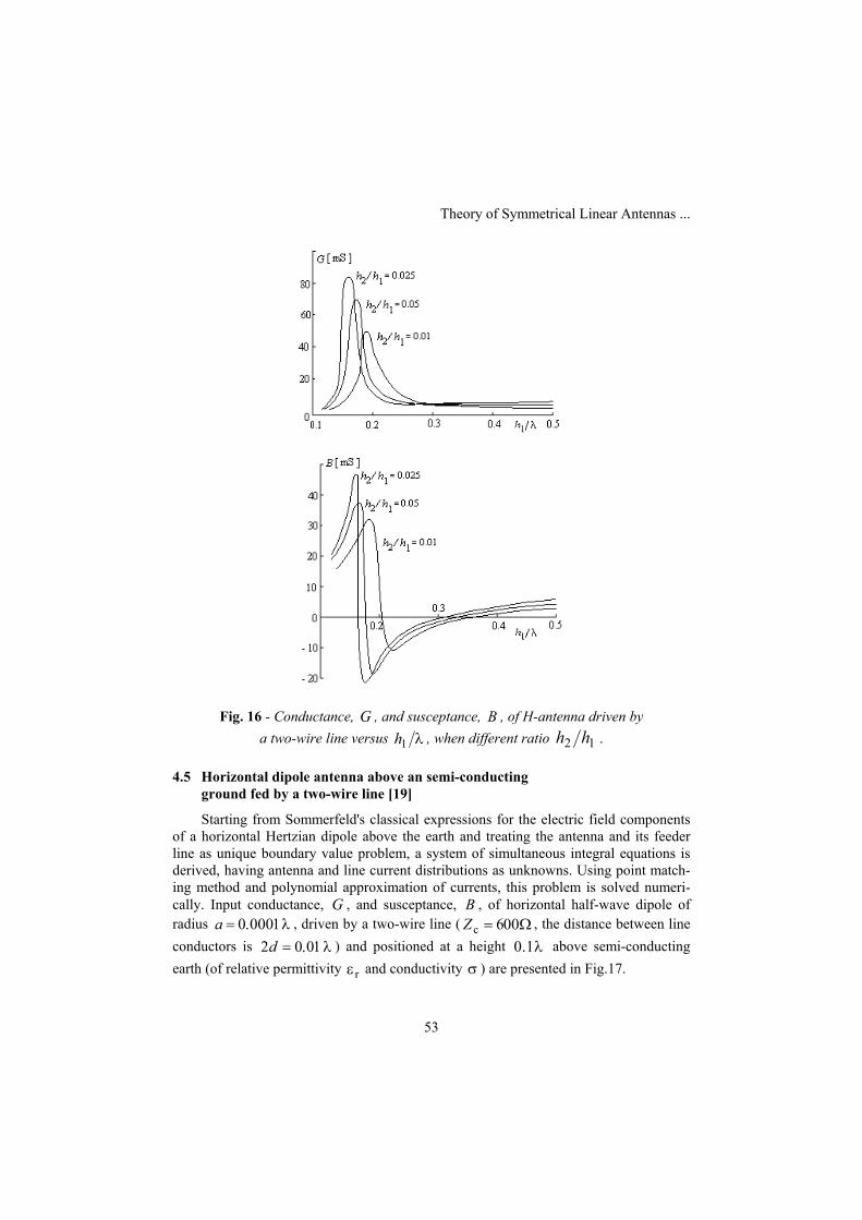
Conductance, G , and susceptance, B , of H-antenna driven by a two-wire line, when

λ0.25== LD , Ω300=cZ , ( )[ ] 10=−2=Ω 121ln ahh , 12 aa =

and different ratio 12 hh versus λ1h is presented in Fig.16.


52

Fig. 14 - H-antenna driven by a two-wire line.

Fig. 15 - Conductance, G , and susceptance, B , of H-antenna driven by a two-wire line

and by delta-function generator, versus λ1h .


53

Fig. 16 - Conductance, G , and susceptance, B , of H-antenna driven by a two-wire line versus λ1h , when different ratio 12 hh .

4.5 Horizontal dipole antenna above an semi-conducting ground fed by a two-wire line [19]

Starting from Sommerfeld's classical expressions for the electric field components of a horizontal Hertzian dipole above the earth and treating the antenna and its feeder line as unique boundary value problem, a system of simultaneous integral equations is derived, having antenna and line current distributions as unknowns. Using point match-ing method and polynomial approximation of currents, this problem is solved numeri-cally. Input conductance, G , and susceptance, B , of horizontal half-wave dipole of radius λ0.0001=a , driven by a two-wire line ( Ω00= 6cZ , the distance between line conductors is λ0.01=d2 ) and positioned at a height λ1.0 above semi-conducting earth (of relative permittivity rε and conductivity σ ) are presented in Fig.17.


54

Fig. 17 - Conductance, G , and susceptance, B , of horizontal half-wave dipole antenna positioned above semi-conducting ground and feed by a two-wire line.

5. Conclusion The investigators of the department of theoretical electromagnetics of Faculty of

Electronic Engineering of Ni suggested one original and very exact theoretical ap-proach to the problem of the symmetrical linear antennas driven by a two-wire line. This method treats the antenna and the transmission line as a unique boundary-value problem leading to a system of two simultaneous integral equations, containing current distribu-tion on the antenna and line conductors as unknowns. These integral equations have been approximately solved using the so-called point matching method and the polyno-mial approximation of the unknown currents on the antenna and on the line. In order to overcome the difficulties, caused by the mutual coupling between the antenna and the transmission line, a new, suitable defined apparent driving-point admittance has been introduced and calculated.


55

The described method has been used to calculate the apparent admittance for sev-eral types of antennas: Centre driven symmetrical dipole antenna, Centre-driven V-an-tenna, Cage antenna, H-antenna and System of two parallel non-staggered dipoles an-tennas in free space or near ground. A remarkable dependence of the admittance on the respect to distance between the transmission line conductors, as well as the inadequacy of the commonly used, idealized delta-function generator have been found. Excellent agreement of theoretical and experimental results for admittance available in the litera-ture has been established.

Using this procedure, several magisterial and doctoral thesis and several tenth of papers were realized on the Faculty of Electronics of Nish.

These results were noticed in scientific area. So the authors in prestige book [27] declare:

"Surutka and Veli~kovi (1976) looked at the problem of solving a practically fed dipole antenna. A two-wire line was used and integral equations derived both on the surface of the dipole conductors and of the surface of the line conductors. This gave simultaneous integral equations containing the current distributions on both the lines and the dipoles and these were solved".

6 Appendix Magnetic vector-potential of a semi-infinite two-wire line carrying progressive current waves

Consider a semi-infinite two-wire line, beginning at 0=y (Fig.18) and ending at infinity ( ∞→y ). Let the line carry the progressive current wave

( ) kyIyI ji e= , (34)

travelling in the negative direction of −y axis.

Fig. 18 - Notation for semi-infinite two-wire line.

With the proximity effect disregarded, the currents can be located on the axes of the wires and the vector-potential at a point ( )yrr ,,M 21 , out of the conductors, can be written in the form


56

yRR

IAkRkRL

kyy ′

−

π4µ

−=−−

0 ∫ deee2

j

1

j

0

ji

21, (35)

where

( )2211 yyrR ′−+= , ( )22

22 yyrR ′−+= ,

1r and 2r being the bipolar coordinates of the point M in the transverse plane y .

Introducing the new variable yyu −′= ( y is assumed to be finite) and by denot-ing the new limits of the integral by yp −= and ∞→q , the integral (35) can be put in the form

+−

+π4µ

−= ∫∫

+−

+−

0 uur

uur

IAq

p

urukq

p

urukky

y dedee22

2

j

221

jj

i

222

221

. (36)

By a new change of the variable

+−= 22 urukt , (37)

tur

tt dd22 +

−=

reads

−π4

µ−= ∫∫

+−

+−

+−

+−

0 tt

tt

IA

qrqk

prpk

kqrqk

prpk-

kky

y dedee

222

222

221

221

jjj

i

tt.

Since

∫ ∫∫ ∫ ∫ ∫∫ ∫ −=−−+=−c

a

d

b

b

a

c

b

c

b

d

c

b

a

d

c

,

the integral in the square bracket in (37) can be written as follows


57

tt

tt

JJJ

qrqk

qrqk

kqrpk

prpk

kdede

222

221

222

221

jj

21 ∫∫

+−

+−

+−

+−

−=−=tt

. (38)

Taking into account that yp −= , and putting, for abbreviation,

++−= 22

101 yrykY ,

+−−= 22

202 yrykY ,

the integral 1J can be expressed in terms of sine- and cosine-integral functions:

( ) ( ) ( ) ( )[ ]01020102

j

1 SiSijCiCide02

01

YYYYY

Y

t−+−== ∫ t

tJ , (39)

where

( ) tt

txx

dcosCi ∫∞

= , ( ) tt

txx

dsinSi ∫∞

= .

The second part of the integral (38) can be evaluated by the help of the mean value theorem:

22

1

222j

2 lneqrq

qrqJ P

+−

+−= , (40)

where

+−≤≤

+− 22

222

1 qrqkPqrqk . (41)

When ∞→q , 0→P and

1

222

1

222

2 lnlnlimrr

qrq

qrqJ

q2=

+−

+−=

∞→. (42)

If on the same semi-infinite two-wire line ( ∞<≤ y0 ), a progressive current wave of the form


58

( ) kyIyI jr e−−= (43)

is present (the wave propagates in the positive direction of the −y axis), the vector-potential can be derived in a similar way and it has the following form

( ) ( ) ( ) ( )[ ] 03040304j

r SiSijCiCie YYYY −−−π4

µ= −0 ky

y IA ,

where

++−= 22

103 yrykY ,

++−= 22

204 yrykY . (44)

5 References [1] R. F. Harrington: Field computation by moment methods, Collier-Macmillan, New

York, 1968. [2] B. D. Popovi: Polynomial approximation of current along thin symmetrical

cylindrical dipoles, Proc. Inst. Elect. Engrs, 117, No. 5, pp. 873 - 8, 1970. [3] D. M. Veli~kovi: A new polynomial approach to the numerical solution of thin

cylindrical antenna problem, Archiv für Elektr., B. 55, 1973, pp. 233 - 236. [4] D. M. Veli~kovi: Thin cylindrical centre driven dipole antenna in non-linear semi-

conducting medium, FACTA UNIVERSITATIS (Nish), Series: Electronics and En-ergetics, No 1 (1991), pp. 155 - 162.

[5] J. V. Surutka, D. M. Veli~kovi: Current and admittance of a symmetric centre-driven V-antenna, Publications de la Faculté d'électrotechnique de 1'Université à Belgrade, Series: Electronique, No. 79, 1973, pp. 21 - 31.

[6] J. V. Surutka, D. M. Veli~kovi: Jedan novi pristup problemu kru`ne okvirne an-tene, Zbornik radova XVIII Jugoslovenske konferencije za ETAN, Ulcinj, juni 1974, pp. 349 - 357.

[7] J. V. Surutka, D. M. Veli~kovi: Kru`na okvirna antena optereena koncentrisanim impedansama, Zbornik radova XVIII Jugoslovenske konferencije za ETAN, Ulcinj, juni 1974, pp. 341- 347.

[8] D. M. Veli~kovi, D. M. Petkovi: A New Integral Equation Method for Thin-Wire Curvilinear Antennas Designing, EURO ELECTROMAGNETICS, EUROEM'94, 30 May - 4 June 1994, Bordeaux, WEp-02-05.

[9] D. M. Veli~kovi, Z. @. Panti: Thin-wire antennas in the presence of a perfectly-conducting body of revolution, The Radio and Electronic Engineer., Vol. 52, No 6, pp. 297 - 303, June 1982.

[10] D. M. Veli~kovi, V. Javor: Computer Package for Analysis of Lightning Elec-tromagnetic Field Distribution for Cage Conductor Structures, Proceedings of Pa-


59

pers, International Conference on Lightning Protection ICLP 2002, 2 - 6 September 2002, Cracow, Poland, pp. 382 - 387.

[11] J. V. Surutka, D. M. Veli~kovi: Input impedance of rectangular V - dipole antenna derived by variational method, Publications de la Faculté d'électrotechnique de 1'Université à Belgrade, Serie: Mathematique et Physique, No 247 - 273, 1969, pp. 87 - 95.

[12] J. V. Surutka, D. M. Veli~kovi: Variational approach to V-dipole antenna analysis, The Radio and Electronic Engineer, Vol. 44, No. 7, July 1974, pp. 367 - 372.

[13] J. V. Surutka, D. M. Veli~kovi: Kru`na okvirna antena: varijacioni postupak sa polinomskom aproksimacijom struje, Zbornik radova XXI Juugoslovenske konfer-encije za ETAN, Banja Luka, juni 1977, Vol. II, pp. 240 - 247.

[14] J. V. Surutka, D. M. Veli~kovi: Admittance of a dipole antenna driven by a two-wire line, The Radio and Electronic Engineer., Vol. 46, No. 3, March 1976, pp. 121 - 128.

[15] J. V. Surutka, D. M. Veli~kovi: Theory of the V-dipole antenna driven by a two-wire line, Publications de la Faculté d'électrotechnique de 1'Université à Belgrade, Series: Electronics, No 102 - 106, 1976, pp. 31 - 46.

[16] J. V. Surutka, D. M. Veli~kovi: Self and mutual admittance/impedance of two parallel no staggered dipoles driven by 2-wire lines, Electronics Letters, 27th May 1976, Vol. 12, No 11, pp. 286 - 287.

[17] J. V. Surutka, D. M. Veli~kovi: Sopstvene i vzaimnie provodnosti (impedansi) dvuh paralelnih neeelonirovanih simetri~nih vibratorov, pitaemih s pom~u dvuh-provodnoj linii, Ekspres informacije, Radiotehnika svevrhvisokih ~astot, No 18, 1977, Moskva, pp. 10 - 13.

[18] J. V. Surutka, D. M. Veli~kovi: Sopstvene i me|usobne impedanse/admitanse spregnutih paralelnih dipola, napajanih dvo`i~nim vodovima, Zbornik radova XX Jugoslovenske konferencije za ETAN, Opatija, juni 1976, pp. 453 - 462.

[19] J. V. Surutka, D. N. Miti: Horizontal dipole antenna above an imperfectly conduct-ing ground fed by a two-wire line, Bulletin T. LXXVIII de l'Academie serbe des sci-ences et des arts, Classe des sciences technique, No 19, Belgrade 1981, pp.1 - 14.

[20] J. Vlaji: Odre|ivanje impedansi dve spregnute nejednake dipol antene napajane dvo`i~nim vodom, M. Sc. thesis, Faculty of Electronic Eng., Ni, 1977.

[21] Z. @. Panti: Cage dipole antenna driven by a two-wire line, AEÜ, Bd. 33, H. 7/8, 1979, pp. 329 - 330.

[22]P. Ran~i: H-antenna driven by a two-wire line, Proc. of XXI ETAN, Belgrade, 1977, pp. II. 245 - 252.

[23] R. W. P. King: The Theory of Linear Antennas, Harvard University Press, Cam-bridge, Mass., 1956.

[24] M. B. Dragovi, J. V. Surutka: Input impedance measurements of symmetrically driven antennas, Proc. of the 19-th Yugoslav Conference on Electronics, Telecom-munications, Automatics and Nuclear Engineering (ETAN), June 1975, Ohrid.


60

[25] D. M. Veli~kovi: Evaluation of integrals appearing in numerical solution of thin cylindrical antenna problems, Publications de la Faculté d'électrotechnique de 1'Uni-versité à Belgrade, Series: Math. and Phys, No 544 - 576, 1976, pp. 81 - 84.

[26] G. M. Milovanovi, D. M. Veli~kovi: Quadrature Processes for Several Types of Quasi-Singular Integrals Appearing in the Electromagnetic Field Problems, Proc. of Full Papers of 5th International Conference on Applied Electromagnetics PES2001, Ni, October 8 - 10 2001, pp. 117 - 122.

[27] Advances in Electronic and Electron Physics, Edited by L. Marton, Smithsonian Institution, Washington, D. C., Academic Press, New York, San Francisco, London, Volume 47, 1978, pp. 129.

[28] E. Hallen: Theoretical investigations into transmitting and receiving antennae, Nova Acta Regiae Soc. Sci. Upsaliensis, Ser. 4, 2, p. 1, 1938.

[29] R. W. P. King, D. Middleton: The cylindrical antenna: current and impedance, Quart. Appl. Math., 3, pp. 302 - 35, 1946.

[30] R. E. Collin, P. J. Zucker: Antenna Theory, Pt. 1, pp. 312 - 4, McGraw-Hill, New York, 1969.

[31] R. W. P. King: The linear antenna-eighty years of progress, Proc. IEEE, 55, No. 1, pp. 2 - 16, 1967.

[32] R. W. P. King, T. T. Wu: On the admittance of a mono-pole driven from a coaxial line, IEEE Trans. on Antennas and Propagation, AP - 17, pp. 814 - 7, 1969.

[33] K. Iizuka, R. W. P. King: Terminal-zone corrections for a dipole driven by a two-wire line, J. Res. Nat. Bur. Stds, 66, D (Radio Prop.), pp. 775 - 82, 1962.

[34] T. T. Wu, R. W. P. King: Driving point and input admittance of linear antennas, J. Appl. Phys., 30, pp. 74 - 6, 1959.

[35] R. H. Duncan: Theory of the infinite cylindrical antenna including the feed-point singularity in the antenna current, Res. Nat. Bur. Stds, 66, D (Radio Prop.), pp. 569 - 84, 1962.

Documents

Symmetrical Linear Antennas Driven by Two-Wire Lines