Symmetric instability in the Gulf Stream

Leif N. Thomasa,⇤, John R. Taylorb, Ra↵aele Ferraric, Terrence M. Joyced

aDepartment of Environmental Earth System Science,Stanford UniversitybDepartment of Applied Mathematics and Theoretical Physics, University of Cambridge

cEarth, Atmospheric and Planetary Sciences, Massachusetts Institute of TechnologydDepartment of Physical Oceanography, Woods Hole Institution of Oceanography

Abstract

Analyses of wintertime surveys of the Gulf Stream (GS) conducted aspart of the CLIvar MOde water Dynamic Experiment (CLIMODE) revealthat water with negative potential vorticity (PV) is commonly found withinthe surface boundary layer (SBL) of the current. The lowest values of PV arefound within the North Wall of the GS on the isopycnal layer occupied byEighteen Degree Water, suggesting that processes within the GS may con-tribute to the formation of this low-PV water mass. In spite of large heatloss, the generation of negative PV was primarily attributable to cross-frontadvection of dense water over light by Ekman flow driven by winds with adown-front component. Beneath a critical depth, the SBL was stably strat-ified yet the PV remained negative due to the strong baroclinicity of thecurrent, suggesting that the flow was symmetrically unstable. A large eddysimulation configured with forcing and flow parameters based on the obser-vations confirms that the observed structure of the SBL is consistent with thedynamics of symmetric instability (SI) forced by wind and surface cooling.The simulation shows that both strong turbulence and vertical gradients indensity, momentum, and tracers coexist in the SBL of symmetrically unstablefronts.

SI is a shear instability that draws its energy from geostrophic flows. Aparameterization for the rate of kinetic energy (KE) extraction by SI appliedto the observations suggests that SI could result in a net dissipation of 33 mWm�2 and 1 mW m�2 for surveys with strong and weak fronts, respectively.The surveys also showed signs of baroclinic instability (BCI) in the SBL,

⇤Corresponding author address: 473 Via Ortega, Stanford CA. 94305, Email address:leift@stanford.edu (Leif Thomas)

Preprint submitted to Deep Sea Research II February 19, 2012

namely thermally-direct vertical circulations that advect biomass and PV.The vertical circulation was inferred using the omega equation and used toestimate the rate of release of available potential energy (APE) by BCI.The rate of APE release was found to be comparable in magnitude to thenet dissipation associated with SI. This result points to an energy pathwaywhere the GS’s reservoir of APE is drained by BCI, converted to KE, andthen dissipated by SI and its secondary instabilities. Similar dynamics arelikely to be found at other strong fronts forced by winds and/or cooling andcould play an important role in the energy balance of the ocean circulation.

Keywords: fronts, subtropical mode water, upper-ocean turbulence, oceancirculation energy

1. Introduction

It has long been recognized that baroclinic instability plays an impor-tant role in the energetics of the Gulf Stream (GS) (e.g. Gill et al., 1974).The instability extracts available potential energy (APE) from the currentconverting it to kinetic energy (KE) on the mesoscale. Turbulence on themesoscale is highly constrained by the Earth’s rotation and thus follows aninverse cascade, with KE being transferred away from the small scales whereviscous dissipation can act (Ferrari and Wunsch, 2009). Thus the pathwayalong which the energy of the GS is ultimately lost cannot be direct throughthe action of the mesoscale alone. Submesoscale instabilities have been im-plicated as mediators in the dissipation of the KE of the circulation as theycan drive a forward cascade (Capet et al., 2008; Molemaker et al., 2010). Onesubmesoscale instability that could be at play in the GS and that has beenshown to be e↵ective at removing KE from geostrophic currents is symmetricinstability (SI) (Taylor and Ferrari, 2010; Thomas and Taylor, 2010).

In the wintertime, the strong fronts associated with the GS experienceatmospheric forcing that makes them susceptible to SI. A geostrophic currentis symmetrically unstable when its Ertel potential vorticity (PV) takes theopposite sign of the Coriolis parameter as a consequence of its vertical shearand horizontal density gradient (Hoskins, 1974). The strongly baroclinicGS is thus preconditioned for SI. SI is a shear instability that extracts KEfrom geostrophic flows (Bennetts and Hoskins, 1979). Under destabilizingatmospheric forcing (i.e. forcing that tends to reduce the PV) the rate of KEextraction by SI depends on the wind-stress, cooling, and horizontal density

2

gradient (Taylor and Ferrari, 2010; Thomas and Taylor, 2010).Preliminary analyses of observations from the eastern extension of the

GS taken during the winter as part of the CLIvar MOde water Dynamic Ex-periment (CLIMODE, e.g. Marshall and Coauthors (2009)) suggest that SIwas present (Joyce et al., 2009). In this article CLIMODE observations thatsampled the GS in both the east and west will be analyzed to characterizethe properties of SI in the current and its e↵ects on the surface boundarylayer. Particular emphasis will be placed on assessing the relative contribu-tions of SI and baroclinic instability to the energy balance of the GS understrong wintertime forcing. Both the energetics and boundary layer dynamicsthat will be discussed are shaped by small-scale turbulent processes. Whilemicrostructure measurements were made as part of CLIMODE (e.g. Inoueet al., 2010), these processes were not explicitly measured during the surveysdescribed here, therefore to study their properties a large eddy simulation(LES) configured with flow and forcing parameters based on the observationshas been performed. Before presenting the analyses of the observations andLES an overview of the dynamics of wind and cooling forced SI will be given.

2. Dynamics of forced symmetric instability

2.1. Potential vorticity and overturning instabilities

A variety of instabilities can develop when the Ertel potential vorticity(PV), q, takes the opposite sign of the Coriolis parameter (Hoskins, 1974),i.e.

fq = f(fk +r⇥ u) ·rb < 0, (1)

where f is the Coriolis parameter, u is the velocity, and b = �g⇢/⇢o isthe buoyancy (g is the acceleration due to gravity and ⇢ is the density). Theinstabilities that arise take di↵erent names depending on whether the verticalvorticity, stratification, or baroclinicity of the fluid is responsible for the lowPV. For barotropic flows where f⇣absN2 < 0 (⇣abs = f �uy + vx) and N2 > 0the instabilities that arise are termed inertial or centrifugal. Gravitational

instability occurs when N2 < 0. In strongly baroclinic flows, the PV can takethe opposite sign of f even if f⇣absN2 > 0. This is illustrated by decomposingthe PV into two terms

q = qvert + qbc, (2)

one associated with the vertical component of the absolute vorticity and thestratification

qvert = ⇣absN2, (3)

3

the other attributable to the horizonal components of vorticity and buoyancygradient

qbc =

✓@u

@z� @w

@x

◆@b

@y+

✓@w

@y� @v

@z

◆@b

@x. (4)

Throughout the rest of the paper we assume that the flows we are consideringare to leading order in geostrophic balance. For a geostrophic flow, ug, it canbe shown using the thermal wind relation that (4) reduces to

qgbc = �f

����@ug

@z

����2

= � 1

f|rhb|2, (5)

so that fqgbc is a negative definite quantity, indicating that the baroclinicityof the fluid always reduces the PV. When |fqgbc| > fqvert, with fqvert > 0,the instabilites that develop are termed symmetric instability (SI).

The instability criterion can equivalently be expressed in terms of the bal-anced Richardson number. Namely, the PV of a geostrophic flow is negativewhen its Richardson number

RiB =N2

(@ug/@z)2⌘ f 2N2

|rhb|2 (6)

meets the following criterion

RiB <f

⇣gif f⇣g > 0 (7)

where ⇣g = f +r⇥ ug · k is the vertical component of the absolute vorticityof the geostrophic flow (Haine and Marshall, 1998). In condition (7) wehave excluded barotropic, centrifugal/inertial instability which arises whenf⇣g < 0. If we introduce the following angle

�RiB

= tan�1

✓� |rhb|2

f 2N2

◆, (8)

instability occurs when

�RiB

< �c ⌘ tan�1

✓�⇣gf

◆. (9)

This angle is not only useful for determining when instabilities occur butit can also be used to distinguish between the various instabilities that canresult. These instabilities can be di↵erentiated by their sources of KE whichvary with �Ri

B

.

4

2.2. Energetics

The overturning instabilities that arise when fq < 0 derive their KE froma combination of shear production and the release of convective availablepotential energy (Haine and Marshall, 1998). The relative contributions ofthese energy sources to the KE budget di↵ers for each instability. For abasic state with no flow and an unstable density gradient, pure gravitationalinstability is generated that gains KE through the buoyancy flux

BFLUX = w0b0 (10)

(the overline denotes a spatial average and primes the deviation from thataverage). With stable stratification, no vertical shear, and f⇣g < 0, cen-trifugal/inertial instability forms and extracts KE from the laterally-shearedgeostrophic current at a rate given by

LSP = �u0v0s ·@ug

@s, (11)

where s is the horizontal coordinate perpendicular to the geostrophic flow andvs is the component of the velocity in that direction. For a geostrophic flowwith only vertical shear, N2 > 0, and fq < 0 SI develops and extracts KEfrom the geostrophic flow at a rate given by the geostrophic shear production

GSP = �u0w0 · @ug

@z. (12)

For an arbitrary flow with fq < 0, depending on the strength and sign of thestratification and vertical vorticity, and the magnitude of the thermal windshear the instabilities that result can gain KE through a combination ofthe buoyancy flux and shear production terms (11)-(12). A linear instabilityanalysis applied to a simple basic state with fq < 0 described in the appendixillustrates that the partitioning between energy sources is a strong function of�Ri

B

and �c. As schematized in figure 1 and described below these two anglescan thus be used to distinguish between the various modes of instability.

For unstable stratification (N2 < 0) and �180� < �RiB

< �135�, grav-itational instability develops, with BFLUX/GSP � 1, while for �135� <�Ri

B

< �90�, a hybrid gravitational/symmetric instability develops, whereboth the buoyancy flux and GSP contribute to its energetics.

For stable stratification and cyclonic vorticity (i.e. ⇣g/f > 1) the insta-bility that forms when

�90� < �RiB

< �c, with �c < �45� (13)

5

derives its energy primarily via GSP and thus can be characterized as SI.For N2 > 0 and anticyclonic vorticity (i.e. ⇣g/f < 1) both the LSP andGSP contribute to the energetics of the instabilities in varying degrees de-pending on �Ri

B

. Specifically, GSP/LSP > 1 and SI is the dominant modeof instability when

�90� < �RiB

< �45�, with �c > �45� (14)

When �45� < �RiB

< �c, a hybrid symmetric/centrifugal/inertial instabilitydevelops, where both the GSP and LSP contribute to its energetics.

In this sense, �RiB

is analogous to the Turner angle which is used to dif-ferentiate between the gravitational instabilities: convection, di↵usive con-vection, and salt fingering that can arise in a water column whose densityis a↵ected by both salinity and temperature (Ruddick, 1983). The param-eter �Ri

B

is also useful because it e↵ectively remaps an infinite range ofbalanced Richardson numbers, �1 < RiB < 1, onto the finite interval�180� < �Ri

B

< 0�.

2.3. Finite amplitude symmetric instability

As with many instabilities that have reached finite amplitude, turbulencegenerated by SI eventually adjusts the background flow so as to push thesystem to a state of marginal stability (Thorpe and Rotunno, 1989). For SIthis corresponds to a geostrophic flow with q = 0, a balanced Richardsonnumber

Riq=0 =f

⇣g(15)

and non-zero stratification

N2q=0 =

|rhb|2f⇣g

. (16)

This is in contrast to finite-amplitude pure gravitational instability which setsthe PV to zero by homogenizing density (Marshall and Schott, 1999). SI andits secondary instabilities drive the PV towards zero by mixing waters withoppositely signed PV together. SI in the SBL thus leads to a restratificationof the mixed layer. It should be noted that the upper ocean can be restratifiedby baroclinic instability as well, but via a di↵erent mechanism: the release ofavailable potential energy by eddy-driven overturning which can occur evenif fq > 0 (Fox-Kemper et al., 2008).

6

In pushing the system to a state with q = 0, SI damps itself out (Taylorand Ferrari, 2009). SI can be sustained however if it is forced by winds orbuoyancy fluxes that generate frictional or diabatic PV fluxes at the surfaceof the ocean that tend to drive fq < 0 and thus compensate for PV mixingby SI (Thomas, 2005; Taylor and Ferrari, 2010). Changes in PV are causedby convergences/divergences of a PV flux:

@q

@t= �r · J, (17)

J = uq +rb⇥ F � (fk +r⇥ u)D, which has an advective component andtwo non-advective constituents arising from frictional or non-conservativeforces, F , and diabatic processes, D ⌘ Db/Dt (Marshall and Nurser, 1992).Therefore in the upper ocean, the necessary condition for fq to be reducedand forced SI (FSI) to be sustained is

f (JzF + Jz

D) |z=0 > 0, (18)

where the vertical components of the frictional and diabatic PV fluxes are

JzF = rhb⇥ F (19)

andJzD = �⇣absD. (20)

When (18) is met, PV is extracted from (injected into) the ocean in theNorthern (Southern) Hemisphere thus pushing the PV in the surface bound-ary layer (SBL) towards the opposite sign of f . As shown in Thomas (2005),(18) can be related to the atmospheric forcing and horizontal density gradi-ent. Specifically, FSI can occur if

EBF + Bo > 0 (21)

where Bo is the surface buoyancy flux and EBF = Me ·rhb|z=0 is the Ekman

buoyancy flux, (Me = ⌧w ⇥ z/⇢of is the Ekman transport), the measureof the rate at which Ekman advection of buoyancy can re- or destratifythe SBL (Thomas and Taylor, 2010). From thermal wind balance, EBF =⇢�1o |⌧w||@ug/@z|z=0| cos ✓, where ✓ is the angle between the wind vector and

geostrophic shear. Therefore, in the absence of buoyancy fluxes, condition(21) is satisfied when the winds have a down-front component, i.e. �90� <✓ < 90�.

7

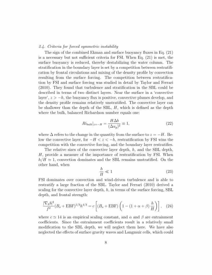
2.4. Criteria for forced symmetric instability

The sign of the combined Ekman and surface buoyancy fluxes in Eq. (21)is a necessary but not su�cient criteria for FSI. When Eq. (21) is met, thesurface buoyancy is reduced, thereby destabilizing the water column. Thestratification in the boundary layer is set by a competition between restratifi-cation by frontal circulations and mixing of the density profile by convectionresulting from the surface forcing. The competition between restratifica-tion by FSI and surface forcing was studied in detail by Taylor and Ferrari(2010). They found that turbulence and stratification in the SBL could bedescribed in terms of two distinct layers. Near the surface in a ‘convectivelayer’, z > �h, the buoyancy flux is positive, convective plumes develop, andthe density profile remains relatively unstratified. The convective layer canbe shallower than the depth of the SBL, H, which is defined as the depthwhere the bulk, balanced Richardson number equals one:

Ribulk|z=�H =H�b

(�ug)2⌘ 1, (22)

where� refers to the change in the quantity from the surface to z = �H. Be-low the convective layer, for �H < z < �h, restratification by FSI wins thecompetition with the convective forcing, and the boundary layer restratifies.

The relative sizes of the convective layer depth, h, and the SBL depth,H, provide a measure of the importance of restratification by FSI. Whenh/H ' 1, convection dominates and the SBL remains unstratified. On theother hand, when

h

H⌧ 1 (23)

FSI dominates over convection and wind-driven turbulence and is able torestratify a large fraction of the SBL. Taylor and Ferrari (2010) derived ascaling for the convective layer depth, h, in terms of the surface forcing, SBLdepth, and frontal strength:

|rhb|2f 2

(Bo + EBF)1/3h4/3 = c

(Bo + EBF)

✓1� (1 + ↵ + �)

h

H

◆�, (24)

where c ' 14 is an empirical scaling constant, and ↵ and � are entrainmentcoe�cients. Since the entrainment coe�cients result in a relatively smallmodification to the SBL depth, we will neglect them here. We have alsoneglected the e↵ects of surface gravity waves and Langmuir cells, which could

8

play an important role in the turbulence of the SBL for conditions where thefriction velocity u⇤ =

p|⌧w|/⇢o is weaker than the Stokes drift (McWilliamset al., 1997).

In order to illustrate the role of frontal baroclinicity, it is useful to rewrite(24) in terms of the velocity scales associated with the surface forcing andthermal wind:

✓h

H

◆4

� c3✓1� h

H

◆3 ✓w3

⇤|�ug|3 +

u2⇤

|�ug|2 cos✓◆2

= 0, (25)

where w⇤ = (BoH)1/3 is the convective velocity and �ug = |@ug/@z|H is thechange in geostrophic velocity across the SBL, and ✓ is the wind angle definedabove. For strongly baroclinic flows, where �ug � u⇤ and �ug � w⇤,

h

H! c3/4

w3

⇤|�ug|3 +

✓u2⇤

|�ug|2◆cos ✓

�1/2⌧ 1, (26)

and restratification by FSI dominates convection. In general, given the sur-face forcing and frontal strength, Eq. (25) can be solved for h/H.

The scaling expression in Eq. (25) provides a useful test for FSI based onobserved conditions. First, by measuring the PV or the balanced Richardsonnumber, RiB, the SBL depth, H, can be identified. Then, using the surfaceforcing and geostrophic shear, Eq. (25) can be used to predict whether FSIwill be active, and the qualitative structure of the vertical density profile.If h/H ' 1, FSI is not expected to be active, and the SBL should be un-stratified. However, if h/H < 1, FSI is possible, and a stable stratification isexpected to develop for �h < z < �H. In Section 3 we will use the predictedconvective layer depth, h, and the observed density and velocity profiles totest for FSI in the GS.

3. Observational evidence of symmetric instability in the Gulf Stream

Diagnostics were performed on the high-resolution SeaSoar/ADCP ob-servations collected as part of CLIMODE to probe for evidence of SI in theGS. The diagnostics entailed calculating the various instability criteria for SI,i.e. (13)-(14), (21), and (23). The analyses were performed on two surveysdenoted as survey 2 and 3. Survey 2 was to the east near the location whereflow detrains from the GS and enters the recirculation gyre and where the

9

GS front is relatively weak. Survey 3 was to the west where the GS front isstrong and has a prominent warm core (Fig. 2).

Representative cross-stream sections of density and PV for the two sur-veys are shown in figure 3(c)-(d). The PV was calculated assuming thatcross-front variations in velocity and density are large compared to along-front variations. On both sections there are regions where the PV was neg-ative. To determine if the dominant mode of instability in these regions wasSI, �Ri

B

was calculated. The parameter �RiB

is especially sensitive to thestratification since it involves calculating N�2, a quantity that can be quitelarge in the weakly stratified surface boundary layer. Thus to make as repre-sentative an estimate of N2 as possible, ungridded profiles of density from theSeaSoar surveys were used to calculate the vertical density gradient at high-resolution. The gridded density fields were used to estimate |rhb|2, whichwere then interpolated onto the cross-stream and vertical positions of theSeaSoar profiles to obtain high-resolution estimates of �Ri

B

. Values of �RiB

that satisfy criteria (13)-(14) were isolated and their locations are highlightedin figure 3(e)-(f). The collocation of waters with q < 0 that satisfy criteria(13)-(14) on the sections indicates that the negative PV is associated withstable stratification, strong baroclinicity, and thus a symmetrically unstableflow.

As described in section 2.3, mixing of PV by SI increases the PV of theboundary layer and hence stabilizes the flow unless the current is driven bybuoyancy loss and/or an EBF which induce PV fluxes that satisfy (18). Ship-board meteorology was used to calculate the net heat flux and EBF. Profilesof the EBF and heat loss are shown in figures 3 (a)-(b). The atmosphericforcing was much stronger on survey 3, with wind-stress values ranging from0.2-0.9 N m�2 and net heat fluxes of order 1000 W m�2. The EBF was highlyvariable across survey 3, reflecting changes in the frontal structure. At theNorth Wall of the GS the EBF was more than an order of magnitude largerthan surface heat flux, with a peak equivalent to 12000 W m�2 of heat loss.Not surprisingly, under such strong destabilizing forcing the PV at the GS isnegative down to over 100 m. While the forcing was weaker on survey 2, witha heat loss of a few hundred W m�2 and an EBF that did not exceed 1000W m�2, regions of negative PV correspond to peaks in the EBF, suggestinga causal link between the forcing and the observed PV distribution.

Apart from destabilizing forcing and a flow with negative PV, the condi-tion for FSI to be the dominant mode of instability is for the convective layerto be shallower than the surface boundary layer. To test this criterion, the

10

depths of both layers were estimated for each survey. The thickness of thesurface boundary layer, H, was estimated using the bulk, balanced Richard-son number criterion (22). The sum of the Ekman and surface buoyancyfluxes, the surface cross-front buoyancy gradient, and the surface boundarylayer depth were used to estimate the convective layer depth, h, by solving(25). The depths of both layers are indicated in figure 3(e)-(f). On bothsurveys there are locations where h is significantly smaller than H. Theseregions tend to coincide with fronts where �Ri

B

falls in the SI range (13)-(14) and the sum of the Ekman and surface buoyancy fluxes is positive, andthus where all three criteria for SI are satisfied. While these observationsare suggestive of SI, the evidence is still somewhat circumstantial becausemore definitive measures of SI and the turbulence that it generates (suchas the turbulent dissipation rate e.g. D’Asaro et al. (2011)) were not col-lected on the surveys. To determine if the conditions observed in the GSwere conducive for SI and to quantify the energy transfer associated with theinstabilities that could have been present, a high resolution large eddy simu-lation (LES) was conducted with initial conditions and forcing representativeof the observations.

4. Large eddy simulation of forced symmetric instability

The configuration of the LES, which is schematized in Figure 4, is meantto be an idealized representation of the flow and forcing along a subsectionof survey 3, line 3. The initial stratification, lateral density gradient, and thesurface forcing were based on averages of the observed fields from survey 3,line 3 collected between 0 and -15 km in the cross-stream direction (see theleft hand panel of Figure 3). More specifically, the density field was initializedusing a piecewise linear buoyancy frequency, shown in Figure 5, that captureskey features of the observed stratification. The initial mixed layer depth is73m and stratification, N2

0 (z), increases rapidly with depth below the mixedlayer before reaching a maximum buoyancy frequency squared of 6.5⇥10�5s�2

at a depth of 125m. In order to speed the development of frontal circulations,we initialized the cross-front buoyancy field with a sinusoidal perturbation:

b(x, z, t = 0) =

ZN2

0dz +M2

x+

LX

2⇡sin

✓2⇡x

LX

◆�. (27)

Although the strength of the front is not uniform across the domain, peri-odic boundary conditions can still be used after subtracting the background

11

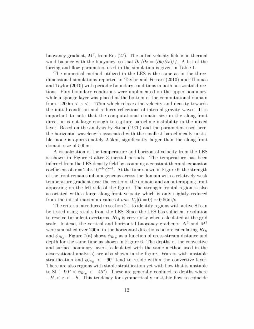
buoyancy gradient, M2, from Eq. (27). The initial velocity field is in thermalwind balance with the buoyancy, so that @v/@z = (@b/@x)/f . A list of theforcing and flow parameters used in the simulation is given in Table 1.

The numerical method utilized in the LES is the same as in the three-dimensional simulations reported in Taylor and Ferrari (2010) and Thomasand Taylor (2010) with periodic boundary conditions in both horizontal direc-tions. Flux boundary conditions were implimented on the upper boundary,while a sponge layer was placed at the bottom of the computational domainfrom �200m < z < �175m which relaxes the velocity and density towardsthe initial condition and reduces reflections of internal gravity waves. It isimportant to note that the computational domain size in the along-frontdirection is not large enough to capture baroclinic instability in the mixedlayer. Based on the analysis by Stone (1970) and the parameters used here,the horizontal wavelength associated with the smallest baroclinically unsta-ble mode is approximately 2.5km, significantly larger than the along-frontdomain size of 500m.

A visualization of the temperature and horizontal velocity from the LESis shown in Figure 6 after 3 inertial periods. The temperature has beeninferred from the LES density field by assuming a constant thermal expansioncoe�cient of ↵ = 2.4⇥10�4�C�1. At the time shown in Figure 6, the strengthof the front remains inhomogeneous across the domain with a relatively weaktemperature gradient near the center of the domain and an outcropping frontappearing on the left side of the figure. The stronger frontal region is alsoassociated with a large along-front velocity which is only slightly reducedfrom the initial maximum value of max|Vg|(t = 0) ' 0.56m/s.

The criteria introduced in section 2.1 to identify regions with active SI canbe tested using results from the LES. Since the LES has su�cient resolutionto resolve turbulent overturns, RiB is very noisy when calculated at the gridscale. Instead, the vertical and horizontal buoyancy gradients, N2 and M2

were smoothed over 200m in the horizontal directions before calculating RiBand �Ri

B

. Figure 7(a) shows �RiB

as a function of cross-stream distance anddepth for the same time as shown in Figure 6. The depths of the convectiveand surface boundary layers (calculated with the same method used in theobservational analysis) are also shown in the figure. Waters with unstablestratification and �Ri

B

< �90� tend to reside within the convective layer.There are also regions with stable stratification yet with flow that is unstableto SI (�90� < �Ri

B

< �45�). These are generally confined to depths where�H < z < �h. This tendency for symmetrically unstable flow to coincide

12

with regions where there is a significant gap between the convective andsurface boundary layers is also seen in the observations (figure 3).

A more quantitative comparison between the observations and the LEScan be made by comparing representative profiles of the balanced Richard-son number. This was done by calculating cross-stream means of N2 and|rhb|, averaged along surfaces of constant z/H, (denoted as hN2i and hM2i,respectively) that were then used to compute a mean, balanced Richardsonnumber, hRiBi ⌘ hN2if 2/hM2i2. Observations from survey 3, line 3 col-lected between cross-stream distances of -15 km and 0 km were used in thecomparison since the initial conditions and forcing of the LES were basedon this data. The temporal evolution of hRiBi from the LES is illustratedin figure 8. Within three inertial periods and beneath the convective layer,the SBL transitions from being unstratified to stably stratified in spite of thedestabilizing forcing, a consequence of the restratifying tendency of SI. In thisrelatively short period of time the profile of hRiBi approximately reaches asteady state, with a vertical structure that resembles the observations giventhe scatter in the data. This suggests that the bulk properties of the SBLseen in the observations are consistent with a flow undergoing FSI.

An important consequence of SI is that energy is extracted from a bal-anced front, converted to three-dimensional turbulent kinetic energy (TKE),and ultimately molecular dissipation. In order to determine the relativeimportance of this source of TKE to the boundary layer turbulence, we cancompare the geostrophic shear production (GSP) with other sources of TKE.Figure 9 shows several possible sources of TKE diagnosed from the LES. Nearthe surface, the wind stress generates TKE through the ageostrophic shearproduction (ASP) term where

ASP = �u0w0 ·✓@u

@z� @ug

@z

◆. (28)

The ASP is large near the surface where it is nearly balanced by the dis-sipation, while its vertically averaged contribution is small as argued byTaylor and Ferrari (2010). The two remaining terms which contribute tothe vertically-integrated TKE production are the buoyancy flux, b0w0, andthe GSP. Positive values of the buoyancy flux indicate convective conditions,which in this case are caused by a combination of the unstable surface buoy-ancy flux, B0, and the Ekman buoyancy flux (EBF). Although the buoyancyflux is a significant source of TKE due to the strong forcing conditions, theGSP is even larger, especially in the lower half of the low PV layer where it

13

dominates the TKE production. This implies that the extraction of frontalkinetic energy may be an important source of turbulence in the GS.

We can use these results from the LES to develop a parameterization forthe GSP. To begin, we invoke the theoretical scaling of Taylor and Ferrari(2010) that the sum of the GSP and BFLUX is a linear function of depth:

GSP +BFLUX ⇡ (EBF +Bo)

✓z +H

H

◆. (29)

By writing an approximate expression for the buoyancy flux profile, we canuse Eq. (29) to derive an expression for the GSP. Assuming that the buoyancyflux is a linear function of depth inside the convective layer, and zero below,

BFLUX ⇡⇢

b0w0 ⇡ Bo(z + h)/h z > �h0 z < �h

, (30)

the GSP can be parameterized with the following expression

GSP ⇡8<

:

(EBF + Bo)�z+HH

�� Bo

�z+hh

�z > �h

(EBF + Bo)�z+HH

� �H < z < �h0 z < �H

. (31)

The parameterizations for the buoyancy flux, GSP, and their sum comparefavorably to the LES results both in their vertical structure and amplitude(figure 9).

5. Sources and sinks of kinetic energy in the Gulf Stream

The submesoscale and mesoscale currents that make up the Gulf Streamgain KE primarily through the release of available potential energy. Asdescribed above, these baroclinic currents are potentially susceptible to SIwhich can act as a sink of KE. In this section we attempt to quantify thesesinks and sources of KE using the observations.

5.1. Removal of kinetic energy from the Gulf Stream by symmetric instability

It is thought that western boundary currents such as the GS lose their KEprimarily through bottom friction at the western boundary. The extractionof KE by SI in the surface boundary layer of western boundary currents isa break from this paradigm. We will estimate this KE sink by calculatingthe net dissipation associated with SI using the shipboard meteorology and

14

SeaSoar hydrography and the parameterization for the GSP (31). We willalso characterize the conditions that result in high frontal dissipation.

Dissipation by SI will be particularly large at strong lateral density gradi-ents forced by down-front winds where the EBF is large. Thus, a collocationof frontogenetic strain and an alignment of the winds with a frontal jet willconspire to give very large KE extraction by SI. A horizontal flow with fron-togenetic strain results in an increase in the lateral buoyancy gradient at arate given by the frontogenesis function:

Ffront ⌘ 2Q ·rhb =D

Dt|rhb|2 (32)

where

Q =

✓�@u@x

·rhb,�@u@y

·rhb

◆(33)

is the so-called Q-vector (Hoskins, 1982). The frontogenesis function wasevaluated on survey 3 using only the geostrophic component of the velocityin Eq. (33). The geostrophic velocity was inferred using density and velocityobservations and constraining ug to satisfy the thermal wind balance and tobe horizontally non-divergent following the method of Rudnick (1996)1.

The near-surface distribution of Ffront is shown in figure 10(a). Strongfrontogenesis (Ffront ⇠ 1 ⇥ 10�17 s�5) occurs in the North Wall of the GSnear the top of line 3 of the survey. To put this value in perspective, as fluidparcels transit the region of frontogenetic strain where Ffront ⇠ 1⇥10�17 s�5,which is around 25 km wide, moving at ⇠ 1 m s�1 (a speed representative ofthe GS in the North Wall) their horizontal buoyancy gradient would increaseby 5⇥ 10�7 s�2.

Previous studies have found that frontogenesis also occurs on a smallerscale driven by wind-forced ageostrophic motions (Thomas and Lee, 2005;Taylor and Ferrari, 2010; Thomas and Taylor, 2010) and in the LES de-scribed above, the frontogenesis driven by SI rivals that associated with thegeostrophic flow estimated from the observations. Frontogenetic circulationcan be seen in the visualization shown in figure 6 as a convergent cross-front velocity at the surface near the region with the strongest temperature

1The velocity and density fields used in the calculation were objectively mapped usingthe method of Le Traon (1990). Each field minus a quadratic fit was mapped at each depthusing 5% noise and an anisotropic Gaussian covariance function with e-folding lengths of20 and 10 km in the along- and cross-stream directions, respectively.

15

gradient. A cross-section of the frontogenesis function, evaluated from theLES is shown in Figure 10(b). Note that here, the full velocity has beenused in evaluating the frontogenesis function instead of just the geostrophiccomponent. The frontogenesis function is very large near the surface at thestrongest front at x ' 1.5km, indicating that the frontogenetic strain fieldsin the LES and observations are comparable in magnitude.

In addition to the intense frontogenesis inferred from the observations,the wind-stress is down-front and large in magnitude (e.g. 10(a)). Both ofthese conditions conspired to amplify the EBF at the North Wall, resultingin the peak value equivalent to 12000 W m�2 of heat loss seen in figure 3(a).On the south wall of the warm core, the flow is also frontogenetic but thewinds are up-front and are not conducive for driving SI. Upfront winds actto restratify the water column, increasing the PV, which tends to suppress SIand its associated extraction of KE. Therefore when averaged laterally overan area where the winds are both up and down front, SI will result in a netremoval of KE from the frontal circulation.

The rate of KE removal by SI was estimated by averaging the parame-terization for the GSP (31) over the area spanned by survey 3. As shownin figure 11, the average GSP peaks at the surface and decays with depth,extending to over 250 m, a depth set by the thick SBLs near the North Wall(e.g. figure 3(a)). Integrated over depth the average GSP (multiplied bydensity) amounts to 33 mW m�2. The contribution to the GSP from wind-forcing alone is assessed by setting Bo = 0 in (31). Wind forcing results in adepth integrated GSP of 27 mW m�2, suggesting that down-front winds arethe dominant trigger for SI on this survey.

On survey 2, both the fronts and atmospheric forcing were weaker (e.g.figure 3), which would imply weaker SI and a reduced GSP. Indeed the pa-rameterization for the GSP (31) averaged over survey 2 is over an order ofmagnitude smaller than that on survey 3 (compare figures 14 and 11). Inte-grated over depth, the net GSP is 1 mW m�2, which is close to the value forwind-forcing alone, namely 0.9 mW m�2.

5.2. Removal of available potential energy from the Gulf Stream by baroclinic

instability

While SI can draw KE directly from the GS, the current also loses avail-able potential energy (APE) to BCI. The GS’s APE loss translates to a KEgain for BCI at a rate given by the buoyancy flux

I = w0b0xy

(34)

16

(where the overline denotes a lateral average over the area of the survey andprimes the deviation from that average). We attempt to quantify this sourceof KE by calculating the the buoyancy flux following a method similar tothat employed by Naveira Garabato et al. (2001) of using a vertical velocityfield inferred by solving the omega equation

f 2@2w

@z2+N2r2

hw = 2r ·Qg, (35)

here written in its quasi-geostrophic form where r2h is the horizontal Lapla-

cian and the subscript “g” indicates that the Q-vector in (35) is evaluatedusing the geostrophic velocity (Hoskins et al., 1978)

The omega equation was solved for survey 3 with w set to zero at theboundaries of the domain over which the computation was made. Settingw = 0 at the bottom of the domain is somewhat of an arbitrary constraintoften used in studies of frontal vertical circulation that can a↵ect the solutionaway from the boundaries (e.g. Pollard and Regier, 1992; Allen and Smeed,1996; Rudnick, 1996; Thomas et al., 2010). Therefore, it is critical to pushthe bottom of the domain as far from the region of interest as possible so thatthe inferred w is not greatly a↵ected by the boundary condition. Thereforethe computational domain for the omega equation calculation was extendedbeneath the SeaSoar survey down to 1000 m. Deep CTD casts taken as partof CLIMODE were used to estimate N2 beneath the SeaSoar survey, and theQ-vector was set to zero at these depths. The divergence of the Q-vectoris largest in magnitude near the surface where frontogenesis is most intense.Thus setting Qg = 0 at depths beneath the SeaSoar survey does not greatlya↵ect the solution to (35) in the near-surface region of interest.

Plan view and cross-stream sections of w for survey 3 are shown in fig-ures 12 and 13. As to be expected, in regions of frontogenesis the verticalcirculation is thermally direct, with downwelling and upwelling on the denseand less dense sides of the front, respectively. The strong frontogenetic strainwhere line 3 intersects the Northern Wall of the GS results in a downdraftwith a magnitude of over 100 m day�1 that extends through the ⇠ 300 mSBL to the north of the GS. This downdraft is coincident with the plumeof low PV and high fluorescence evident in figures 3(c) and 13. Conversely,regions of upwelling correspond to areas of low fluorescence and high PV(e.g. near -10 km in the cross-stream direction). The correlation betweenthe fluorescence, PV, and w suggests that three dimensional processes suchas baroclinic instability play a key role in the vertical exchange of biomass

17

and PV across the pycnocline. As described in Joyce et al. (2009), a simi-lar correlation between low PV, enhanced fluorescence, and high oxygen wasobserved on survey 2.

Using the solution to the omega equation, the buoyancy flux (34) wasestimated across the area spanned by survey 3 (e.g. figure 11). Above z ⇡�200 m, w0b0

xyis positive, implying that APE is being extracted from the GS

over this range of depths. The buoyancy flux peaks near z ⇡ �50 m whichis within the SBL (e.g. figure 3(a)). While the positive buoyancy flux issuggestive of BCI, other process that drive a net thermally-direct circulation(such as large-scale frontogenetic strain) could have been present as well.

To determine whether the buoyancy flux estimated using the omega equa-tion is consistent with the energetics of BCI, the buoyancy flux associatedwith BCI was inferred using the parameterization of Fox-Kemper et al. (2008)

w0BCIb

0BCI

x=

Ce(Hx)2|rhb

xz|2|f | µ(z) (36)

where ()zand ()

xindicates an average across the SBL and in the along-front

direction, respectively, Ce ⇡ 0.06 is an empirically determined coe�cient,and µ(z) is a vertical structure function that goes to zero at the top andbottom of the SBL. The parameterization (36) captures the vertical modeof BCI confined to the SBL associated with submesoscale mixed layer eddies(MLEs) (Boccaletti et al., 2007; Fox-Kemper et al., 2008). Low vertical modeBCIs with a deeper extension could also contribute to the buoyancy flux butare not parameterized by (36).

The density field averaged in the along-stream direction was used to eval-uate (36). The cross-stream average of w0

BCIb0BCI

xhas similar features to

w0b0xy

in the upper 200 m (figure 11). The zero crossing of the buoyancy fluxassessed using the vertical velocities from the omega equation is close to thedepth where w0

BCIb0BCI

xaveraged across the survey goes to zero. The two

buoyancy fluxes have maxima near 50 m that are of similar strength. Giventhe potential errors that could arise in calculating the correlation betweenw and b over a survey that spans only a few submesoscale meanders of theGS, the agreement between the two estimates for the buoyancy flux suggeststhat the inferred APE release in the upper 200 m of the GS is qualitativelyconsistent with the energetics of baroclinic instability. When integrated overthis depth range, the net buoyancy flux (multiplied by density) is estimatedas 23 mW m�2 and 15 mW m�2 using (34) and (36), respectively. Thesevalues are smaller yet similar to the net GSP associated with SI.

18

On survey 2 an estimate of the APE release by BCI using the omegaequation diagnostic could not be performed due to gaps in the velocity dataand the relatively coarse along-front resolution of the survey. However, thebuoyancy flux associated with BCI could be assessed using the parameteriza-tion (36). In spite of the deeper SBLs, owing to the weaker fronts of survey2, w0

BCIb0BCI

xis over an order of magnitude weaker than that estimated for

survey 3 (figure 14). The parameterization suggests that the net APE releaseby BCI amounts to 1 mW m�2, equivalent to the inferred net dissipation bySI on the survey. Therefore based on these observations we can conclude thatunder the strong wintertime forcing experienced on the surveys, SI plays acomparable role to BCI in the energetics of the GS.

6. Conclusions

High resolution hydrographic and velocity surveys of the Gulf Streammade during strong wintertime forcing evidence a symmetrically unstablecurrent with negative PV caused by cooling and down-front winds. In spiteof the large wintertime heat loss, a combination of frontogenetic strain asso-ciated with the geostrophic flow combined with down-front winds conspiredto make the winds, through the Ekman advection of buoyancy, the dominantcause for decrease in PV. The lowest PV observed in the surveys is foundon the EDW isopycnal layer where it outcrops at the North Wall of the GSunder the maximum in the EBF.

These observations may shed light on the question as to why EDW formson the isopycnal layer bounded by the 26.4 and 26.5 kg m�3 density surfaces.The observations reveal that in the winter it is these density surfaces thatoutcrop in the North Wall of the GS where the horizontal density gradient ofthe open-ocean Northwest Atlantic is persistently strong (Belkin et al., 2009).Combined with a down-front wind, the outcrop of EDW isopycnal layer in theNorth Wall also coincides with a maximum in frictional PV removal whichcauses the PV to be preferentially reduced on this layer. This is indeed whatis observed on survey 3. While frictional PV fluxes can locally dominate overdiabatic PV fluxes along the fronts of the GS, PV budgets for the EDW isopy-cnal layer calculated using a coarse-resolution, data-assimilating numericalsimulation suggest that when integrated over the entire outcrop area, heatloss rather than friction is the primary mechanism for the seasonal reductionof the volume integrated PV on the layer (Maze and Marshall, 2011). Thisdoes not necessarily imply that frontal processes are unimportant for EDW

19

formation. Cooling dominates the PV budgets because it covers a larger out-crop area than wind-driven frictional PV fluxes. The large outcrop areas areto a large degree a reflection of the subsurface structure of the stratificationand low PV anomalies that precondition the fluid for deep convective mixedlayers. Thus processes that lead to the generation and subduction of waterwith anomalously low PV, such as those observed on the North Wall of theGS described here and in Thomas and Joyce (2010), can contribute indirectlyto the formation of EDW and thus select the isopycnal layer on which it isfound.

A large eddy simulation configured with flow and forcing parametersbased on the observations reveals that the destabilizing winds and buoyancyloss generate a deepening SBL with negative PV yet with stable stratifica-tion across a large fraction of its thickness. The turbulence in this stratifiedlayer derives its energy from both the buoyancy field and the geostrophicflow. In the LES the rate of KE extraction from the geostrophic flow bythe turbulence scales with the EBF and surface buoyancy flux in agreementwith a simple parameterization for SI. While PV is well mixed in the SBL,buoyancy, momentum, and tracers retained significant vertical structure inspite of strong turbulence with dissipation rates exceeding 1⇥ 10�6 W kg�1.

These results have important implications for the parameterization ofturbulent mixing in the upper ocean. The traditional view is that turbu-lence near the sea surface is driven solely by atmospheric forcing (winds orbuoyancy fluxes). Our analysis shows that turbulence can also be generatedthrough frontal instabilities. In addition, current parameterizations take aone dimensional view where vertical mixing spans a boundary layer whosedepth is commonly computed using a bulk Richardson number criterion (e.g.the KPP mixing scheme of Large et al. (1994) and the PWP model of Priceet al. (1986)). The critical bulk Richardson number used to determine theboundary layer depth is typically less than one, i.e. lower than the thresh-old for SI. Consequently at a front undergoing SI these mixing schemes willunder predict the depth of the boundary layer. A second, and perhaps moreimportant problem is that many models based on bulk criteria either assumeuniform water mass properties in the boundary layer, or assign a very largevertical di↵usivity. However, in observations taken during CLIMODE andthe LES, vertical gradients of buoyancy, momentum, and tracers persist inthe symmetrically unstable boundary layer. Vertical mixing is not strongenough to maintain a homogeneous boundary layer in the face of restratifica-tion. As shown by Taylor and Ferrari (2011) this has important consequences

20

for the biology as well as the physics of the upper ocean, especially in thehigh latitudes where the strength of vertical mixing can determine the meanlight exposure and hence growth rate of phytoplankton.

Apart from evidencing SI, the observational surveys of the GS show signsof baroclinic instability, namely thermally direct vertical circulations that re-lease available potential energy and advect tracers such as biomass and PV.These signatures of baroclinic instability are strongest in the surface bound-ary layer and are characterized by submesoscale length scales, suggestingthat the instabilities are a form of the mixed layer eddies (MLEs) modeledby Boccaletti et al. (2007) and Fox-Kemper et al. (2008). While baroclinicinstability injects kinetic energy into the geostrophic flow, symmetric insta-bility extracts KE, transferring it to small scales where it can be dissipated byfriction (Thomas and Taylor, 2010). The observations suggest that the ratesof KE removal and injection by the two instabilities averaged over the sur-face boundary layer are of the same order of magnitude. This result impliesthat SI can limit or prevent the inverse cascade of KE by MLEs and pointsto an energy pathway where the Gulf Stream’s reservoir of APE is drainedby MLEs, converted to KE, then dissipated by SI and its secondary insta-bilities. It follows that this energy pathway would be preferentially openedduring the winter, when strong atmospheric forcing both deepens the SBL,which allows for energetic MLEs to develop, and reduces the PV in frontalregions, triggering SI.

The depth-integrated dissipation associated with SI inferred from surveys2 and 3 was 1 mW m�2 and 33 mW m�2, respectively. This range of netdissipation is similar to that observed in the abyss of the Southern Ocean,O(1)�O(10) mW m�2, which has been ascribed to the breaking of internalwaves generated by geostrophic currents flowing over rough topography, aprocess thought to remove about 10% of the energy supplied by winds to theglobal circulation (Naveira Garabato et al., 2004; Nikurashin and Ferrari,2010). In contrast to breaking of internal waves however, dissipation associ-ated with SI in the SBL is likely to exhibit a seasonal cycle and thus averagedannually will result in weaker net dissipation values. Having said this, recentobservations in the Kuroshio taken during late spring have revealed local netdissipation rates of ⇠ 100 mW m�2 at a symmetrically unstable front drivenby weak atmospheric forcing, with minimal buoyancy loss and wind-stressmagnitudes of less than 0.2 N m�2 (D’Asaro et al., 2011). The intense dissi-pation at the Kuroshio was attributable to the combination of an extremelysharp front and the down-front orientation of the wind which resulted in

21

an EBF large enough to explain the observed dissipation. Thus SI and theKE extraction it induces is not solely a wintertime phenomenon, however itis confined to frontal regions which are limited in area. The contribution ofdissipation associated with SI to the removal of KE from the entire ocean cir-culation is a challenging number to constrain owing to the dependence of SIon submesoscale frontal features. However, the wintertime observations fromthe GS described here suggest that this contribution could be significant, andthus future studies should aim to quantify it.

Acknowledgments

Thanks are due to all the colleagues in the CLIMODE project, especiallythose organizing this special issue and Frank Bahr at WHOI for his e↵ortsin collecting the hydrographic and velocity measurements with the SeaSoarand shipboard ADCP. Support came from the National Science FoundationGrants OCE-0961714 (LT) and OCE-0959387 (TJ) and the O�ce of NavalResearch Grants N00014-09-1-0202 (LT) and N00014-08-1-1060 (JT and RF).

Appendix. Simple model for gravitational, inertial, and symmetricinstability and their energy sources

The simplest model for studying the overturning instabilities that developwhen fq < 0 consists of a background flow with spatially uniform gradients:ug = (M2/f)z � [(F 2 � f 2)/f ]y, where M2/f is the thermal wind shearand F 2/f = f � @ug/@y is the absolute vorticity of the geostrophic flow,both of which are assumed to be constant. The stratification, N2, is alsospatially uniform and has a value such that the PV of the geostrophic flow,q = (F 2N2�M4)/f takes the opposite sign of f . The governing equation forthe overturning streamfunction of the instabilities (which are assumed to beinvariant in the x-direction and of small amplitude so that their dynamics islinear) is

@2

@t2

✓@2

@y2+

@2

@z2

◆ + F 2@

2

@z2+ 2M2 @

2

@y@z+N2@

2

@y2= 0 (37)

where v0 = @ /@z and w0 = �@ /@y are the instabilities’ meridional andvertical velocities, respectively (Hoskins, 1974). If there are no boundaries,solutions of the form of plane waves = < { exp[�t+ i(ly +mz)]} can besought, where l,m are the components of the wavevector and � is the growth

22

rate. Substituting this ansatz into (37) yields an equation for the growthrate: �2 = �N2 sin2 ↵ � F 2 cos2 ↵ + M2 sin 2↵, where ↵ = � tan�1(l/m) isthe angle that the velocity vector in the y � z plane makes with the hori-zontal. Each mode, with angle ↵ and vertical wavenumber m, has buoyancyand zonal velocity anomalies, (b0, u0) = < {(B,U) exp[�t+ i(ly +mz)]} withamplitudes

B = im

�

�M2 �N2 tan↵

� (38)

U = im

f�

�F 2 �M2 tan↵

� . (39)

The modes that maximimize or minimize the growth rate are characterizedby velocity vectors with angles:

↵0,1 =1

2tan�1

✓2M2

N2 � F 2

◆+⇡

2n n = 0, 1, (40)

where ↵max = max(↵0,↵1) corresponds the angle of the fastest growing mode.The information from this simple linear stability analysis can be used to

estimate the relative strength of the energy sources (10)-(12) of the fastestgrowing overturning instabilities that develop when fq < 0. Namely,

BFLUX

GSP

���↵max

⇠ � w0b0

w0u0(M2/f)

���↵max

= �(M2 �N2 tan↵max)

(F 2 �M2 tan↵max)

✓f 2

M2

◆

(41)LSP

GSP

���↵max

⇠ u0v0(f 2 � F 2)/f

w0u0(M2/f)

���↵max

=(1� F 2/f 2)

tan↵max

✓f 2

M2

◆(42)

The dependence of these ratios on M2 and N2 is shown in figure 15 for abackground flow with anticyclonic vorticity and absolute vorticity F 2/f =0.4f . As can be seen in the figure the ratios are highly dependent of the angle�Ri

B

. The buoyancy flux exceeds the geostrophic shear production only for�Ri

B

less than �135�. Thus below this angle the instability transitions toconvection. For �135� < �Ri

B

� 90� the instability gets its energy primarilyfrom the vertical shear of the geostrophic flow and secondarily from theconvective available potential energy. When the stratification is stable, i.e.�Ri

B

> �90�, the buoyancy flux plays a minimal role in the energetics of theinstabilities. This is because for these values of �Ri

B

the fastest growing modehas flow that is nearly parallel to isopycnals and thus B ⇡ 0. For �90� <

23

�RiB

� 45� the instability gets its energy primarily from the vertical shear ofthe geostrophic flow and secondarily from its lateral shear. Above �Ri

B

=�45�, and for su�ciently strong anticyclonic vorticity, LSP/GSP becomeslarger than one, indicating a transition from symmetric to centrifugal/inertialinstability. The boundaries marking the transitions between gravitational,symmetric, and inertial/centrifugal instability based on this linear stabilityanalysis are schematized in figure 1.

References

Allen, J. T., Smeed, D. A., 1996. Potential vorticity and vertical velocity atthe Iceland-Faeroes front. J. Phys. Oceanogr. 26, 2611–2634.

Belkin, I. M., Cornillon, P. C., Sherman, K., 2009. Fronts in large marineecosystems. Prog. Oceanogr. 81, 223–236.

Bennetts, D. A., Hoskins, B. J., 1979. Conditional symmetric instability - apossible explanation for frontal rainbands. Qt. J. R. Met. Soc. 105, 945–962.

Boccaletti, G., Ferrari, R., Fox-Kemper, B., 2007. Mixed layer instabilitiesand restratification. J. Phys. Oceanogr. 37, 2228–2250.

Capet, X., McWilliams, J. C., Molemaker, M. J., Shchepetkin, A. F., 2008.Mesoscale to submesoscale transition in the California Current system.Part III: Energy balance and flux. J. Phys. Oceanogr. 38, 2256–2269.

D’Asaro, E., Lee, C. M., Rainville, L., Harcourt, R., Thomas, L. N., 2011.Enhanced turbulence and energy dissipation at ocean fronts. Science 332,318–332, doi: 10.1126/science.1201515.

Ferrari, R., Wunsch, C., 2009. Ocean circulation kinetic energy: Reservoirs,sources, and sinks. Annu. Rev. Fluid Mech. 41, 253–282.

Fox-Kemper, B., Ferrari, R., Hallberg, R., 2008. Parameterization of mixedlayer eddies. Part I: Theory and diagnosis. J. Phys. Oceanogr. 38, 1145–1165.

Gill, A. E., Green, J. S. A., Simmons, A. J., 1974. Energy partition in thelarge-scale ocean circulation and the production of mid-ocean eddies. Deep-Sea Res. 21, 499–528.

24

Haine, T. W. N., Marshall, J., 1998. Gravitational, symmetric, and baroclinicinstability of the ocean mixed layer. J. Phys. Oceanogr. 28, 634–658.

Hoskins, B. J., 1974. The role of potential vorticity in symmetric stabilityand instability. Qt. J. R. Met. Soc. 100, 480–482.

Hoskins, B. J., 1982. The mathematical theory of frontogenesis. Annu. Rev.Fluid Mech. 14, 131–151.

Hoskins, B. J., Draghici, I., Davies, H. C., 1978. A new look at the !-equation. Qt. J. R. Met. Soc. 104, 31–38.

Inoue, R., Gregg, M. C., Harcourt, R. R., 2010. Mixing rates across the GulfStream, Part 1: On the formation of Eighteen Degree Water. J. Mar. Res.68, 643–671.

Joyce, T. M., Thomas, L. N., Bahr, F., 2009. Wintertime observations ofSubtropical Mode Water formation within the Gulf Stream. Geophys. Res.Lett. 36, L02607, doi:10.1029/2008GL035918.

Large, W. G., McWilliams, J. C., Doney, S. C., 1994. Oceanic vertical mixing:a review and a model with a nonlocal boundary layer parameterization.Rev. Geophys. 32, 363–403.

Le Traon, P. Y., 1990. A method for optimal analysis of fields with spatiallyvariable mean. J. Geophys. Res. 95(C8), 13543–13547.

Marshall, J., Coauthors, 2009. The Climode field campaign: Observing thecycle of convection and restratification over the Gulf Stream. Bull. Amer.Meteor. Soc. 90, 1337–1350.

Marshall, J., Schott, F., 1999. Open ocean deep convection: observations,models and theory. Rev. Geophys. 37, 1–64.

Marshall, J. C., Nurser, A. J. G., 1992. Fluid dynamics of oceanic thermoclineventilation. J. Phys. Oceanogr. 22, 583–595.

Maze, G., Marshall, J., 2011. Diagnosing the observed seasonal cycle of At-lantic subtropical mode water using potential vorticity and its attendanttheorems. J. Phys. Oceanogr. 41, 1986–1999.

25

McWilliams, J. C., Sullivan, P. P., Moeng, C. H., 1997. Langmuir turbulencein the ocean. J. Fluid Mech. 334, 1–30.

Molemaker, J., McWilliams, J. C., Capet, X., 2010. Balanced and unbalancedroutes to dissipation in an equilibrated Eady flow. J. Fluid Mech. 654, 35–63.

Naveira Garabato, A., Polzin, K., King, B., Heywood, K., Visbeck, M., 2004.Widespread intense turbulent mixing in the Southern Ocean. Science 303,210–213.

Naveira Garabato, A. C., Allen, J. T., Leach, H., Strass, V. H., Pollard,R. T., 2001. Mesoscale subduction at the Antarctic Polar Front driven bybaroclinic instability. J. Phys. Oceanogr. 31, 2087–2107.

Nikurashin, M., Ferrari, R., 2010. Radiation and dissipation of internal wavesgenerated by geostrophic motions impinging on small-scale topography:Application to the Southern Ocean. J. Phys. Oceanogr. 40, 2025–2042.

Pollard, R. T., Regier, L. A., 1992. Vorticity and vertical circulation at anocean front. J. Phys. Oceanogr. 22, 609–625.

Price, J. F., Weller, R. A., Pinkel, R., 1986. Diurnal cycling: observationsand models of the upper ocean response to diurnal heating, cooling, andwind mixing. J. Geophys. Res. 91, 8411–8427.

Ruddick, B. R., 1983. A practical indicator of the stability of the watercolumn to double-di↵usive activity. Deep-Sea Res. 30, 1105–1107.

Rudnick, D. L., 1996. Intensive surveys of the Azores Front. 2. Inferring thegeostrophic and vertical velocity fields. J. Geophys. Res. 101 (C7), 16291–16303.

Stone, P., 1970. On non-geostrophic baroclinic stability: Part II. J. Atmo-spheric Sciences 27, 721–726.

Taylor, J., Ferrari, R., 2009. The role of secondary shear instabilities in theequilibration of symmetric instability. J. Fluid Mech. 622, 103–113.

Taylor, J., Ferrari, R., 2010. Buoyancy and wind-driven convection at mixed-layer density fronts. J. Phys. Oceanogr. 40, 1222–1242.

26

Taylor, J., Ferrari, R., 2011. Ocean fronts trigger high latitude phytoplanktonblooms. Geophys. Res. Lett. 38, L23601.

Thomas, L. N., 2005. Destruction of potential vorticity by winds. J. Phys.Oceanogr. 35, 2457–2466.

Thomas, L. N., Joyce, T. M., 2010. Subduction on the northern and southernflanks of the Gulf Stream. J. Phys. Oceanogr. 40, 429–438.

Thomas, L. N., Lee, C. M., 2005. Intensification of ocean fronts by down-frontwinds. J. Phys. Oceanogr. 35, 1086–1102.

Thomas, L. N., Lee, C. M., Yoshikawa, Y., 2010. The subpolar front of theJapan/East Sea II: Inverse method for determining the frontal verticalcirculation. J. Phys. Oceanogr. 40, 3–25.

Thomas, L. N., Taylor, J. R., 2010. Reduction of the usable wind-work onthe general circulation by forced symmetric instability. Geophys. Res. Lett.37, L18606, doi:10.1029/2010GL044680.

Thorpe, A. J., Rotunno, R., 1989. Nonlinear aspects of symmetric instability.J. Atmos. Sci. 46, 1285–1299.

27

SymmetricInstability

GravitationalInstability

Symmetric/GraviationalInstability

Stable

Inertial/SymmetricInstability

SymmetricInstability

GravitationalInstability

Symmetric/GraviationalInstability

Stable

Anticyclonic vorticity Cyclonic vorticity

Figure 1: Schematic illustrating the relation between the angle �RiB , (8), to the various

overturning instabilities that arise when fq < 0 and the vorticity is anticyclonic (left) andcyclonic (right). The dependence of �

RiB on the baroclinicity and stratification is alsoindicated.

28

SST from Feb 22, 2007

latit

ude

longitude−70 −65 −60 −55 −5035

40

45SST from Mar 8, 2007

latit

ude

longitude−70 −65 −60 −55 −5035

40

45

6 8 10 12 14 16 18 20 22SST (C°)

Figure 2: Satellite-based SST around the time when survey 2 (left) and survey 3 (right)were made (the ship track is in gray). The insets in each figure show the near surfacetemperature as measured during the hydrographic surveys contoured every 1� C. Line 2 ofsurvey 2 corresponds to the middle section. Line 3 of survey 3 is the easternmost section.

29

−4000 0

4000 800012000

(a)

(W m

−2)

survey 3

−400

−300

−200

−100

26.5

26.4

z (m

)

(c)

−20 0 20 40 60

−400

−300

−200

−100

0

(e)

z (m

)

cross−stream distance (km)

−1000 −500

0 500

1000(b)

(W m

−2)

survey 2

26.6

26.5

(d)

−2

−1

0

1

2

PVx1

09 (s−3

)

0 20 40 60 80

−400

−300

−200

−100

0

z (m

)

cross−stream distance (km)

(f)

Figure 3: Observational evidence of SI on survey 3, line 3 (left panels) and survey 2, line 2(right panels). (a)-(b) The cross-front structure of the heat loss (red) and Ekman buoyancyflux, expressed in units of a heat flux (black). Positive values of the EBF and heat fluxindicate conditions favorable for FSI. Cross-stream sections of density (gray contours) andPV (c)-(d) reveal regions where the PV was negative. As shown in (e)-(f) these regionstend to coincide with locations (denoted by the gold dots) where �90� < �

RiB < �45�

in regions of anticyclonic vorticity or �90� < �RiB < �

c

< �45� in regions of cyclonicvorticity. They also lie in areas where the convective layer depth (cyan line) is less thanthe depth of the surface boundary layer (dark blue line) suggesting that the negative PVis associated with FSI.

30

x (km)

z (m

)

1 2 3 -200

-160

-120

-80

-40

0

40

500400

300200

100

y(m)

ThermalWind

Figure 4: Schematic of the LES configuration.

31

1025.5 1025.6 1025.7 1025.8 1025.9 1026��

��

��

��

��

��

�

�

�

�

0(a)

l

Dep

th (m

)

0 2 � 6 8x 10ï�

��

��

��

��

��

��

�

�

�

�

0

Dep

th (m

)

N2 (sï�)

(b)

Figure 5: Initial profiles of (a) density and (b) buoyancy frequency for the large-eddysimulation described in Section 4.

32

Temperature (oC)

0-200m

500 m

1km 2km 3km 4km

-100m

0

Cross-front velocity (cm/s)

0-200m

500 m

1km 2km 3km 4km

-100m

0

Along-front velocity (cm/s)

0-200m

500 m

1km 2km 3km 4km

-100m

0

17.6

17.5

17.4

17.3

40

30

20

10

0

0

5

10

-10

-5

Figure 6: Visualization of the temperature and horizontal velocity fields from the LES.In order to emphasize the regions with larger velocities, the volume visualization of bothvelocity components have been made transparent for |u|, |v| < 2.5cm/s.

33

500 1000 1500 2000 2500 3000 3500 4000��

��

��

��

��

��

�

�

�

�

0

Dep

th (m

)

x (m)0

Figure 7: Cross-front section of �RiB from the LES. The color scheme is the same as that

used in figure 1. The depths of the convective layer (black) and surface boundary layer(cyan) are also indicated.

34

−0.5 0 0.5 1 1.5 2 2.5−1

−0.9

−0.8

−0.7

−0.6

−0.5

−0.4

−0.3

−0.2

−0.1

0

<RiB>=<N2>f2/<M2>2

z/H

Figure 8: The Richardson number of the balanced flow laterally-averaged along surfacesof constant z/H, hRi

B

i, from line 3, survey 3 for cross stream distances between -15 kmand 0 km (red). Profiles of hRi

B

i from the LES averaged between four time periods: t = 0(black), 0 < t < 2⇡/f (blue solid), 2⇡/f < t < 4⇡/f (blue dashed), and 4⇡/f < t < 6⇡/f(blue dashed-dotted) and across the entire computational domain is shown for comparison.

35

ï� ï��� � ��� � [���ï�ï���

��

��

��

��

��

�

�

�

�

�

Dep

th (m

)

ï� � � [���ï�ï���

��

��

��

��

��

�

�

�

�

�

Dep

th (m

)

Figure 9: TKE production terms from the LES (right panel), namely the geostrophicshear production (GSP, solid green), buoyancy flux (BFLUX, solid red), and their sum(solid black), along with the ageostrophic shear production (ASP, cyan) and minus thedissipation (magenta). Each term is averaged over the horizontal domain and for oneinertial period. Parameterizations for the buoyancy flux (red dashed), the GSP (greendashed), and their sum (black dashed) based on Eqns. (29-31) are shown for comparisionin the panel on the left which is an expanded view of the panel on the right. All quantitiesare in units of W kg�1.

36

(a)

x (km)

Fron

toge

nesis

func

tion

(s-5

)

(b)

Figure 10: (a) The density (contours) and frontogenesis function (shades) at z = �44m on survey 3. Vectors represent the wind-stress (for scaling, the maximum magntitudeof the wind-stress is 0.94 N m�2 on the survey). The magneta line is the ship track.Line 3 is the easternmost line of the survey. (b) A cross-section of the density (contours)and frontogenesis function averaged over six hours (shades) from the LES. Since spatialgradients are very large on the scale of three-dimensional turbulence, the velocity andbuoyancy gradients appearing in the frontogenesis function were each averaged across thealong-front direction and smoothed in the along-front direction over a window of 250m.

37

−1.5 −1 −0.5 0 0.5 1 1.5 2 2.5 3 3.5x 10−7

−400

−350

−300

−250

−200

−150

−100

−50

0

(W kg−1)

z (m

)

Figure 11: An estimate for SI’s geostrophic shear production, e.g. (31), attributed toboth wind-forcing and cooling (black) and wind-forcing alone (black dashed) for survey 3.Also shown is the buoyancy flux associated with baroclinic instability estimated using theomega equation diagnostic, w0b0

xy

, (gray) and the parameterization for BCI, (36), (graydashed). All quantities have been averaged laterally over the survey.

38

Figure 12: The density and inferred vertical velocity at z = �44 m on survey 3 calculatedusing the quasigeostrophic omega equation.

39

26.5

26.4

vertical velocity

cross−stream distance (km)

z (m

)

−20 0 20 40 60−400

−300

−200

−100

−20 0 20 40 60−400

−300

−200

−100

fluorescence

cross−stream distance (km)

w (m day−1)−100 −50 0 50 100

Figure 13: The density (contours), inferred vertical velocity (left), and fluorescence (right)on line 3 of survey 3.

40

0 0.2 0.4 0.6 0.8 1 1.2 1.4 1.6x 10−8

−400

−350

−300

−250

−200

−150

−100

−50

0

(W kg−1)

z (m

)

Figure 14: An estimate for SI’s geostrophic shear production, e.g. (31), attributed toboth wind-forcing and cooling (black) and wind-forcing alone (black dashed) for survey 2.Also shown is the buoyancy flux associated with baroclinic instability estimated using theparameterization for BCI, (36), (gray dashed). All quantities have been averaged laterallyover the survey.

41

−3

−2

−10

1

f2N2x1013 (s−4)

−M4 x1

013 (s

−4)

log(BFLUX/GSP)

−10 −5 0 5−12

−10

−8

−6

−4

−2

0

2

−4

−3

−2

−1

0

f2N2x1013 (s−4)

−M4 x1

013 (s

−4)

log(LSP/GSP)

−10 −5 0 5−12

−10

−8

−6

−4

−2

0

2

Figure 15: Logarithm (base ten) of the ratio of the energy source terms for gravitationalinstability, SI, and inertial instability, i.e. (41) and (42), for the fastest growing mode thatforms in a background flow with uniform vertical shear of strength M2/f and absolutevorticity F 2/f = 0.4f , and stratification N2. In the plots the angle measured counter-clockwise from the abscissa is �

RiB . Given the anticyclonic vorticity of the flow, the valueof �

RiB below which the PV turns negative is �c

= �21.8�.

42

Table 1: Parameters for the large-eddy simulation

(LX,LY, LZ) (NX,NY,NZ) M2 Q0

(4km, 500m, 200m) (768,96,50) �1.3⇥ 10�7s�2 1254W/m2

B0 ⌧wx ⌧wy EBF5.3⇥ 10�7m2/s3 �0.20N/m2 �0.48N/m2 6.5⇥ 10�7m2/s3

43