SYMMETRIC FUNCTIONAL DIFFERENTIAL EQUATIONS AND …SYMMETRIC FUNCTIONAL DIFFERENTIAL EQUATIONS AND NEURAL NETWORKS WITH MEMORY JIANHONG WU ... for systems of functional di erential

TRANSACTIONS OF THEAMERICAN MATHEMATICAL SOCIETYVolume 350, Number 12, December 1998, Pages 4799–4838S 0002-9947(98)02083-2

SYMMETRIC FUNCTIONAL DIFFERENTIAL EQUATIONSAND NEURAL NETWORKS WITH MEMORY

JIANHONG WU

Abstract. We establish an analytic local Hopf bifurcation theorem and atopological global Hopf bifurcation theorem to detect the existence and todescribe the spatial-temporal pattern, the asymptotic form and the globalcontinuation of bifurcations of periodic wave solutions for functional differen-tial equations in the presence of symmetry. We apply these general resultsto obtain the coexistence of multiple large-amplitude wave solutions for thedelayed Hopfield-Cohen-Grossberg model of neural networks with a symmetriccirculant connection matrix.

1. Introduction

The purpose of this paper is to study the spatial-temporal patterns of solutionsfor systems of functional differential equations in the presence of symmetry. Ofmajor concern is the existence, the asymptotic form, the isotropy group and theglobal continuation of periodic wave solutions. The well-known Hopfield-Cohen-Grossberg model of neural networks with delay provides the motivation and theillustration of our main general results.

We will start with the symmetric local Hopf bifurcation problem of the followingparametrized system of functional differential equations

x(t) = L(α)xt + f(α, xt),(1.1)

where f(α, 0) = 0 and ∂∂φf(α, 0) = 0 for α ∈ R and φ ∈ C := C([−τ, 0]; Rn),

τ ≥ 0, is a given constant, xt is the usual notation for an element of C defined byxt(s) = x(t + s) with s ∈ [−τ, 0], L : R × C → Rn is continuous and linear in thesecond argument. Moreover, there exists a compact Lie group Γ acting on Rn suchthat f(α, γφ) = γf(α, φ) and L(α)γφ = γL(α)φ for (α, γ, φ) ∈ R × Γ × C, whereγϕ ∈ C is given by (γφ)(s) = γφ(s) for s ∈ [−τ, 0]. We assume that there exists acritical value α0 such that at α = α0, (i). The infinitesimal generator A(α) of theC0-semigroup generated by the linear system x(t) = L(α)xt has a pair of purelyimaginary eigenvalues ±iβ0; (ii) the generalized eigenspace Uiβ0(A(α0)) associatedwith iβ0 consists of eigenvectors of A(α0) only and the restricted action of Γ onUiβ0(A(α0)) is isomorphic to V ⊕ V for some absolutely irreducible representationV of Γ.

Received by the editors September 13, 1995.1991 Mathematics Subject Classification. Primary 34K15, 34K20, 34C25.Key words and phrases. Periodic solution, delay differential equation, wave, symmetry, neural

network, equivariant degree, global bifurcation.Research partially supported by the Natural Sciences and Engineering Research Council of

Canada.

c©1998 American Mathematical Society

4799

License or copyright restrictions may apply to redistribution; see https://www.ams.org/journal-terms-of-use

4800 JIANHONG WU

Under the above assumptions, Uiβ0(A(α0)) consists of ω = 2πβ0

-periodic func-tions and Γ × S1 acts on Uiβ0(A(α0)) by shifting arguments. We will show, inTheorem 2.1, that under usual non-resonance and transversality conditions, for ev-ery subgroup Σ ≤ Γ × S1 such that the Σ-fixed point subspace of Uiβ0(A(α0)) isof dimension 2, system (1.1) has a bifurcation of periodic solutions whose spatio-temporal symmetry can be completely characterized by Σ. In other words, un-der non-resonance and transversality conditions, maximal isotropy groups withminimal-dimensional fixed-point subspaces lead to bifurcations of periodic solutionswith a certain spatio-temporal symmetry.

Note that the presence of symmetry often causes purely imaginary eigenvalues tobe multiple and hence, the standard Hopf bifurcation theory of functional differen-tial equations (cf. Hale [27], Hassard, Kazarinoff and Wan [29]) cannot be applied.Our general result, Theorem 2.1, represents an analog for functional differentialequations of a well-known symmetric Hopf bifurcation theorem established by Gol-ubitsky and Stewart [24] for ordinary differential equations (see also Golubitsky,Stewart and Schaeffer [25] and Vanderbauwhede [54] for a more detailed account ofthe local symmetric Hopf bifurcation theory). However, the proof of this analogueis not an elementary exercise as even the precise statement and verification of thehypotheses of this analog require nontrivial applications of some important facts ofthe generalized eigenspaces of the infinitesimal generators of solution semigroupsand the decomposition theory of linear retarded functional differential equations.

We next consider the global continuation of the bifurcation of symmetric peri-odic solutions detected by the analytic local symmetric Hopf bifurcation theorem(Theorem 2.1). Our strategy here is strongly influenced by the work of Alexanderand Auchmuty [3] where the global continuation of phase-locked oscillations in asystem of ordinary differential equations arising from Turing rings of identical cellswas investigated by considering the maximal continuation of periodic solutions foran associated scalar functional differential equations of mixed type (with both ad-vanced and delayed arguments). More generally, our analytic local symmetric Hopfbifurcation theorem describes the spatio-temporal pattern of the bifurcated periodicsolutions. This spatio-temporal pattern of the bifurcated periodic solutions oftenenables us to obtain a relatively simpler system of functional differential equation ofmixed type and with an additional parameter (usually the period) which completelycharacterizes the bifurcated periodic solutions. In other words, the global contin-uation problem of the bifurcated symmetric periodic solutions of a parametrizedsystem of functional differential equations can be reduced to a corresponding prob-lem of the bifurcated periodic solutions of a relatively simpler system of functionaldifferential equations which is of mixed type and with two parameters, but withoutsymmetry.

With this reduction in mind, we apply the S1-bifurcation theory developed byGeba and Marzantowicz [21] to establish a global Hopf bifurcation theorem, The-orem 3.3, for a system of functional differential equations of mixed type and withtwo parameters. At each stationary solution a sequence of bifurcation invariants,called the crossing numbers, is defined and can be evaluated from the information,via the Brouwer degree, of the linearization of the system at the stationary solution.Our global bifurcation theorem then claims that in the so-called Fuller’s space (cf.Fuller [19]), along each bounded connected component of the nontrivial periodicsolutions, the sum of the aforementioned crossing numbers must be zero.


SYMMETRIC FDES AND NEURAL NETWORKS 4801

Global bifurcation problems have been extensively studied during the last twodecades. A global bifurcation theorem was first established by Rabinowitz [51]for a compact perturbation of the identity parametrized by a real number, andthen generalized to more general classes of nonlinear mappings by Alexander [1],Alexander and Fitzpatrick [4], Dancer [11], Fenske [14], Hetzer and Stallbohm [31],Nussbaum [48] and Stuart [53], to name a few. A similar result was also obtainedfor global continua of periodic solutions of differential equations by Alexander [1],Alexander and Fitzpatrick [4], Alexander and Yorke [5], Chow and Mallet-Paret[8], Chow, Mallet-Paret and Yorke [9], Fiedler [15, 16], Fitzpatrick, [17], Geba andMarzantowicz [21], Ize [35, 36], Ize, Massabo and Vignoli [37, 38], Mallet-Paretand Yorke [46], Nussbaum [49]. We refer to Fielder [15], Ize, Massabo and Vignoli[37, 38] and Erbe, Geba, Krawcewicz and Wu [20] for a detailed account of theliterature.

Our general result, Theorem 3.3, represents an analog of the aforementionedresults, in particular, the results of Alexander and Auchmuty [2], Chow and Mallet-Paret [8], Fiedler [15, 16], Ize [35, 36], Mallet-Paret and Yorke [46] and Nussbaum[49], for functional differential equations of mixed type and with two parameters.This is not strikingly new but provides a crucial tool in our later application tothe existence of large-amplitude wave solutions of delayed neural networks. Itshould be mentioned that in our approach, we employed the S1-equivariant degreeconstructed by Dylawerski, Geba, Jodel and Marzantowicz [12]. There is nowa more general version of the equivariant degree introduced by Ize, Massabo andVignoli [37, 38] and Geba, Krawcewicz and Wu [20] and a corresponding bifurcationtheory developed by Ize, Massabo and Vignoli [37, 38], Krawcewicz, Vivi and Wu[39] and Krawcewicz and Wu [40]. We emphasize that the main contribution ofTheorem 3.3 is to formulate the global bifurcation theory in the setting easilyapplied to the problem of obtaining an unbounded continuation of periodic solutionsof functional differential equations.

In Sections 4 and 5, our general results will be illustrated by their applicationsto the delayed Hopfield-Cohen-Grossberg model of neural networks:

ui(t) = −ui(t) +n∑

j=1

Jijf(uj(t− τ)), 1 ≤ i ≤ n,(1.2)

where f is a sigmoidal function normalized so that f(0) = 0, J = (Jij) is a sym-metric circulant matrix with all the diagonal elements identical to zero. It wasshown by Hopfield [33, 34] and Cohen and Grossberg [10] that every solution of(1.2) is convergent to the set of equilibria if τ = 0. On the other hand, in electronicimplementations of analog neural networks, time delays are present in the com-munication and response of neurons due to the finite switching speed of amplifiers(neurons). Designing a network to operate more quickly increases the relative sizeof the intrinsic delay and may cause sustained oscillations. In particular, Marcusand Westervelt [47] have demonstrated how the neuron gain, delay and the sizeand connection topology of the network affect the existence of oscillatory modesin continuous-time analog neural networks with time delay from the viewpoint oflocal analysis and with the help of numerical integration and some experiments ona small electronic network.


4802 JIANHONG WU

By using Theorem 2.1 and Theorem 3.3, we will show that system (1.2) exhibitsvery rich dynamics and various types of oscillations for large delay. In particular,we will obtain the coexistence of

(i) pitchfork bifurcations of equilibria;(ii) Hopf bifurcations of synchronous oscillations (periodic solutions satisfying

ui(t) = ui−1(t) for i(modn), t ∈ R);(iii) Hopf bifurcations of phase-locked oscillations (periodic solutions satisfying

ui(t) = ui−1(t − rnp), i(modn), t ∈ R, where r ∈ 0, . . . , n − 1 is a given

integer and p > 0 is a period of u);(iv) Hopf bifurcations of mirror-reflecting waves (periodic solutions satisfying

ui(t) = un−i(t), i(modn), t ∈ R);(v) Hopf bifurcations of standing waves (periodic solutions satisfying un−i(t) =

ui(t− 12p), i(modn), t ∈ R, where p > 0 is a period of u).

We will also show that several branches of phase-locked oscillations, standing wavesand mirror-reflecting waves may bifurcate simultaneously from the trivial solutionat some critical values of the delay.

The above wave solutions are special cases of the so-called coherent oscillationobserved by Marcus and Westervelt [47]. In comparison with these results, wenot only can detect the existence of sustained oscillations but also describe theirspatio-temporal patterns. Moreover, as a result of our approach based on globalbifurcation theorems, the coexistence of the aforementioned wave solutions will beestablished for delay not only near but also far away form the critical values. There-fore, we can obtain wave solutions of large amplitudes. We establish such globalexistence results by applying Theorem 3.3 and by (i) obtaining a priori bounds forperiodic solution; (ii) excluding wave solutions of a certain period using the spectralanalysis of Nussbaum [50] for circulant matrices (see Lemma 5.3, Theorem 5.4 andTheorem 6.3).

Depending on the value of the neuron gain (f ′(0)) and the topology and sizeof the interconnection matrix, the aforementioned oscillations can be either stableor unstable. In fact, in Marcus and Westervelt [47] it has been observed thatsome systems of neural networks with delay possess multiple basins of attractionfor coexisting equilibria and oscillatory attractors. Due to the (topological) natureof our approach to the existence of wave solutions we are, in general, unable todiscuss the stability of these waves, except in several special cases where the theoryof monotone dynamical systems of Hirsch [32] and Smith [52] can be applied toexclude stable discrete waves, as will be illustrated in Section 6.

Finally, we mention that existing research has indicated some similarity betweenthe system (1.2) with large delay and the parallel-update network ui(k + 1) =∑n

j=1 Jijf(uj(k)) studied in Frumkin and Moses [18], Goles-Chacc, Fogelman-Soulie and Pellegrin [22], Goles and Vichniac [23], Grinstein, Jayaprakash and He[26], Little [43] and Little and Shaw [44]. We wish to address the related singularperturbation problem in a future paper.

2. Analytic local symmetric Hopf bifurcations for FDEs

Let τ ≥ 0 be a given real number and C denote the Banach space of con-tinuous mapping from [−τ, 0] into Rn equipped with the supremum norm ‖φ‖ =sup−τ≤θ≤0 |φ(θ)| for φ ∈ C. In what follows, if σ ∈ R, A ≥ 0 and x : [σ−τ, σ+A] →



Rn is a continuous mapping, then xt ∈ C, t ∈ [σ, σ+A], is defined by xt(θ) = x(t+θ)for −τ ≤ θ ≤ 0.

Suppose L : R × C → Rn is continuous and linear in the second argument,f : R × C → Rn is continuous and has continuous first and second derivatives inthe second argument with f(α, 0) = 0, αf

αφ (α, 0) = 0 for α ∈ R and φ ∈ C. Considerthe following system of delay differential equations

x(t) = L(α)xt + f(α, xt),(2.1)

where x(t) denotes ddtx(t). It is well-known that for each fixed α, the linear system

x(t) = L(α)xt(2.2)

generates a strongly continuous semigroup of linear operators with the infinitesimalgenerator A(α) given by

A(α)φ = φ, φ ∈ Dom(A(α)),

Dom(A(α)) = φ ∈ C; φ ∈ C, φ(0) = L(α)φ.Moreover, the spectrum σ(A(α)) of A(α) consists of eigenvalues which are solutionsof the following characteristic equation

det∆(α, λ) = 0,(2.3)

where the characteristic matrix ∆(α, λ) is given by

∆(α, λ) = λ Id−L(α)(eλ· Id).(2.4)

We assume(H1) The characteristic matrix is continuously differentiable in α ∈ R and there

exist α0 ∈ R and β0 > 0 such that (i) A(α0) has eigenvalues ±iβ0; (ii) thegeneralized eigenspace, denoted by Uiβ0(A(α0)), of these eigenvalues ±iβ0

consists of eigenvectors of A(α0); (iii) all other eigenvalues of A(α0) are notinteger multiple of ±iβ0.

(H2) There exists a compact Lie group Γ acting on Rn such that both L(α)and f(α, ·) are Γ-equivariant, i.e. f(α, γφ) = γf(α, φ), L(α)γφ = γL(α)φfor (α, γ, φ) ∈ R × Γ × C, where γφ ∈ C is given by (γφ)(θ) = γφ(θ),θ ∈ [−τ, 0].

Note that we do not require the eigenvalues ±iβ0 to be simple. In fact, thepresence of symmetry often causes these purely imaginary eigenvalues to be mul-tiple. Hence, the standard Hopf bifurcation theory of functional differential equa-tions (cf. Hale [27] and Hassard, Kazarinoff and Wan [29]) cannot be applied. Tostate the next assumption, we note that under (H1), Uβ0(A(α0)) is the real vectorspace consisting of Re(eiβ0·b) and Im(eiβ0·b) such that b ∈ Ker∆(α0, iβ0). More-over, there exists a natural identification between Ker∆(α0, iβ0) and R2m, where2m = dim Ker∆(α0, iβ0), as a real vector space. We also require(H3) There exists an m-dimensional absolutely irreducible representation V of Γ

such that Ker∆(α0, iβ0) is isomorphic to V ⊕V , here a representation V ofΓ is absolutely irreducible if the only linear mapping that commutes withthe action of Γ is a scalar multiple of the identity.

Remark 2.1. Assume that (H1)–(H3) are satisfied. Let bj1 + ibj2mj=1 be a basis

for Ker∆(α0, iβ0) and define sinβ , cosβ ∈ C([−τ, 0]; R) by

sinβ(θ) = sin(βθ), cosβ(θ) = cos(βθ), θ ∈ [−τ, 0].


4804 JIANHONG WU

Then the columns of Φα0 = (ε1, . . . , ε2m) form a basis for Uiβ0(A(α0)), where

εj = sinβ bj1 + cosβ bj2,

εm+j = cosβ bj1 − sinβ bj2, 1 ≤ j ≤ m.

It can be easily verified that

A(α0)εj = βεm+j , A(α0)εm+j = −βεj , 1 ≤ j ≤ m.

That is,

AΦα0 = Φα0B(α0),

where

B(α0) =(

0 β Idm

−β Idm 0

)and Idm is the identity matrix of order m.

Remark 2.2. Let

L(α)φ =∫ 0

−τ

[dη(α, θ)]φ(θ), φ ∈ C,α ∈ R,

where η(α, θ) is an n×n matrix function of bounded variation in θ ∈ [−τ, 0]. Then(2.2) can be written as

x(t) =∫ 0

−τ

[dη(α, θ)]x(t + θ).(2.5)

Along with this linear homogeneous equation, we will also consider the formaladjoint equation

y(s) = −∫ 0

−τ

y(s− θ)[dη(α, θ)](2.6)

together with the bilinear form

(ψ, φ)α = ψ(0)φ(0)−∫ 0

−τ

∫ θ

0

ψ(ξ − θ)[dη(α, θ)]φ(ξ) dξ(2.7)

for φ ∈ C and ψ ∈ C∗ := C([0, τ ]; Rn∗), where Rn∗ is the space of n-dimensionalrow vectors. Let A∗(α) denote the infinitesimal generator of the strongly continuoussemigroup generated by (2.6) on C∗. Then the subspace of solutions to the linearalgebraic equation

x∗∆(α0, iβ0) = 0, x∗ ∈ Rn∗ + iRn∗ := Cn∗

has a basis cj1 + icj2mj=1, cj1, cj2 ∈ Rn∗, 1 ≤ j ≤ m. If cos∗β , sin

∗β ∈ C([0, τ ]; R)

are defined by

cos∗β(θ) = cos(βθ), sin∗β(θ) = sin(βθ), θ ∈ [0, τ ],

then Ψ∗α0

= (ε∗1, . . . , ε∗2m) forms a basis for Uiβ0(A

∗(α0)), where

ε∗j = sin∗β cj1 + cos∗β cj2,

ε∗m+j = cos∗β cj1 − sin∗β cj2, 1 ≤ j ≤ m.



Lemma 2.1. Under assumptions (H1)–(H3), there exist δ0 > 0 and a continu-ously differentiable function λ : (α0 − δ0, α0 + δ0) → C such that λ(α0) = iβ0,λ(α) is an eigenvalue of A(α), Uλ(α)(A(α)) consists of eigenvectors of A(α), anddimUλ(α)(A(α)) = dimUiβ0(A(α0)). Moreover, there exist 2m continuously dif-ferentiable mappings ej : (α0 − δ0, α0 + δ0) → C and 2m continuously differen-tiable mappings e∗j : (α0 − δ0, α0 + δ0) → C∗ such that ej(α0) = εj , e

∗j(α0) = ε∗j ,

Φα = (e1(α), . . . , e2m(α)) is a basis of Uλ(α)(A(α)) and Ψα = (e∗1(α), . . . , e∗2m(α))is a basis of Uλ(α)(A∗(α)).

Proof. Let P and I − P denote the projection operators defined by the decompo-sition

Cn = Ker∆(α0, iβ0)⊕ Ran∆(α0, iβ0).

As Ker∆(α0, iβ0) is Γ-invariant, P and I−P commutes with the Γ-action. Rewritethe equation

∆(α, λ)b = 0(2.8)

as ∆(α0, iβ0)d = [I − P ][∆(α0, iβ0)−∆(α, λ)](b0 + d)P [∆(α0, iβ0)−∆(α, λ)](b0 + d) = 0

(2.9)

where

b = b0 + d(2.10)

is the unique decomposition such that

b0 ∈ Ker∆(α0, iβ0), d ∈ Ran∆(α0, iβ0).

Applying the implicit function theorem, we obtain δ1 > 0 and an n × n matrixD∗(α, λ), continuously differentiable for |α − α0| < δ1 and |λ − iβ0| < σ1, suchthat D∗(α0, iβ0) = 0, d = D∗(α, λ)b0 is a solution of the first equation of (2.9), andD∗(α, λ) commutes with the action of Γ on Ker∆(α0, iβ0). Therefore, the existenceof an eigenvalue λ near iβ0 for α near α0 is equivalent to the existence of a solutionof

f(α, λ)b0 = 0,(2.11)

where

f(α, λ)b0 = P [∆(α0, iβ0)−∆(α, λ)][Idm +D∗(α, λ)]b0.

Properly choosing a basis for Cn, we may assume

P =(

Idm 00 0

),∆(α, λ) =

(∆11(α, λ) ∆12(α, λ)∆21(α, λ) ∆22(α, λ)

),

where ∆11(α, λ) is an m×m matrix, ∆22(α, λ) is of order (n−m)× (n−m) and

∆(α0, iβ0) =(

0 00 ∆22(α0, iβ0)

), det∆22(α0, iβ0) 6= 0.

Therefore,

f(α, λ) = −[∆11(α, λ) + ∆12(α, λ)D∗(α, λ)].(2.12)

Moreover, substituting d by D∗(α, λ)b0 in the first equation of (2.9), we get

∆21(α, λ) = −∆22(α, λ)D∗(α, λ).(2.13)


4806 JIANHONG WU

This implies that

∆(α, λ) =(

∆11(α, λ) ∆12(α, λ)−∆22(α, λ)D∗(α, λ) ∆22(α, λ)

)=(

Idm 00 ∆22(α, λ)

)(∆11(α, λ) ∆12(α, λ)−D∗(α, λ) Idm

).

Consequently, from (2.12) it follows that

det∆(α, λ) = (−1)m det ∆22(α, λ) det f(α, λ).(2.14)

As dimUiβ0(A(α0)) = 2m, by the well-known folk theorem for retarded functionaldifferential equations (cf. Hale [27] and Levinger [42]) we have

∂k

∂λk det∆(α0, λ)|λ=iβ0 = 0, 0 ≤ k ≤ m− 1,∂m

∂λm det∆(α0, λ)|λ=iβ0 6= 0.(2.15)

Therefore, as det∆22(α0, iβ0) 6= 0, we derive from (2.14) the following∂k

∂λk det f(α, λ) = 0, 0 ≤ k ≤ m− 1,∂m

∂λm det f(α, λ) 6= 0.(2.16)

On the other hand, under assumption (H3) we may assume

f(α, λ) =(F11(α, λ) F12(α, λ)F21(α, λ) F22(α, λ)

)for some m × m real matrices Fij , i, j = 1, 2. The Γ-equivariance of D∗(α, λ)implies that f(α, λ) commutes with the diagonal action of Γ on V ⊕ V , and henceFij commutes with the action of Γ on V . By the absolute irreducibility of V , wehave

Fij(α, λ) = fij(α, λ) Idm

for some scalar functions fij(α, λ). So

det f(α, λ) = qm(α, λ),

where

q(α, λ) = f11(α, λ)f22(α, λ) − f12(α, λ)f21(α, λ).

By (2.16), we get q(α0, iβ0) = 0, ∂∂λq(α0, λ)|λ=iβ0 6= 0. Therefore, from the implicit

function theorem it follows that there exist δ0 > 0 and a continuous differen-tiable function λ(α) for |α − α0| < δ0 such that λ(α0) = iβ0, q(α, λ(α)) = 0 and|λ(α) − iβ0| < δ1. So, λ(α) is an eigenvalue of A(α) with multiplicity 2m, and thecorresponding eigenvector is

b(α) = [I +D∗(α, λ(α))]b, b ∈ Ker∆(α0, iβ0).

Consequently, dimUλ(α)(A(α)) = dimUiβ0(A(α0)) for |α− α0| < δ0. Let

b∗j1(α) + ib∗j2(α) = [I +D∗(α, λ(α))][bj1 + ibj2].

Then

ej(α) = Im eλ(α)·[b∗j1(α) + ib∗j2(α)],

em+j(α) = Re eλ(α)·[b∗j1(α) + ib∗j2(α)], 1 ≤ j ≤ m,

form a basis of Uλ(α)(A(α)) with the required properties.



The same argument can be applied to construct the basis c∗j1(α) + ic∗j2(α)mj=1

for the subspace of solutions to the equation x∗∆(α, λ(α)) = 0 for x∗ ∈ Rn∗.Therefore,

e∗j (α) = Im eλ(α)·[c∗j1(α) + ic∗j2(α)],

e∗m+j(α) = Re eλ(α)·[c∗j1(α) + ic∗j2(α)], 1 ≤ j ≤ m,

form a basis of Uλ(α)(A∗(α)) with the required properties. This completes theproof.

Remark 2.3. It can be easily shown that

A(α)Φλ(α) = Φλ(α)B(α),

where

B(α) =(

Reλ(α) Idm − Imλ(α) Idm

Imλ(α) Idm Reλ(α) Idm

).

We also need the following

Lemma 2.2. Let (Ψα,Ψα)α = ((e∗j , ek)α)1≤j,k≤2m. Then

B′(α) = −(Ψα,Φα)−1α Ψα(0)

[d

dαL(α)

]Φα.

The proof is similar to that of Lemma 3.9 on pp. 179 of Hale [27] and thereforeis omitted.

Let ω = 2πβ0

. Denote by Pω the Banach space of all continuous ω-periodic map-pings x : R → Rn. Then Γ× S1 acts on Pω by

(γ, θ)x(t) = γx(t+ θ), (γ, θ) ∈ Γ× S1, x ∈ Pω .

Denote by SPω the subspace of Pω consisting of all ω-periodic solutions of (2.2)with α = α0. Then for each subgroup Σ ≤ Γ× S1, the fixed point set

Fix(Σ, SPω) = x ∈ SPω; (γ, θ)x = x for all (γ, θ) ∈ Σis a subspace.

Under assumption (H1), the columns of U(t) = Φα0(0)eB(α0)t, t ∈ R, form abasis for SPω.

Lemma 2.3. SPω is a Γ× S1-invariant subspace of Pω.

Proof. For each γ ∈ Γ, γKer∆(α0, iβ0) ⊆ Ker∆(α0, iβ0). So there exist αγjk and

βγjk, 1 ≤ j, k ≤ m, such that

γbj1 =m∑

k=1

[αγjkbk1 − βγ

jkbk2],

γbj2 =m∑

k=1

[βγjkbk1 + αγ

jkbk2], 1 ≤ j ≤ m.

Let

T1γ = (αγjk)1≤j,k≤m, T2γ = (βγ

jk)1≤j,k≤m.

Then, we can easily verify that

γU(t) = U(t)(T1γ −T2γ

T2γ T1γ

).


4808 JIANHONG WU

So γSPω ⊆ SPω. Moreover, for every θ ∈ S1,

θU(t) = U(t)(

cos θ Idm − sin θ Idm

sin θ Idm cos θ Idm

).

Therefore, θSPω ⊆ SPω. This completes the proof.

Lemma 2.4. Let Tγ = ( T1γ −T2γ

T2γ T1γ) be given in the argument of Lemma 2.3. Then

Γ× S1 acts on R2m by

(γ, θ)w = Tγ

(cos(βθ) Idm − sin(βθ) Idm

sin(βθ) Idm cos(βθ) Idm

)w, w ∈ R2m,

and this action is isomorphic to the restricted action of Γ× S1 on Uiβ0(A(α0)).

Proof. Let w = (w1, . . . , w2m)T ∈ R2m. Then the mapping H : R2m → Uiβ0(A(α0))defined by

Hw =2m∑j=1

wjεj

gives an isomorphism of the representation of R2m and Uiβ0(A(α0)).

Lemma 2.5. Consider the linear nonhomogeneous equation

x(t) = L(α0)xt + g(t).(2.17)

Let

TPω = g ∈ Pω ; (2.17) has an ω-periodic solution.Then TPω is Γ× S1-invariant.

Proof. It is well-known that (2.17) has an ω-periodic solution if and only if∫ ω

0

y(t)g(t) dt = 0

for every ω-periodic solution of the formal adjoint equation (2.6) with α = α0. Onthe other hand, if y(s) is a ω-periodic solution of (2.6) with α = α0, then

y(s)γ = −∫ 0

−τ

y(s− θ)[dη(α0, θ)]γ

= −∫ 0

−τ

y(s− θ)γ[dη(α0, θ)].

So y(s− θ)γ is also an ω-periodic solution of (2.6) with α = α0. Consequently, forevery g ∈ TPω,∫ ω

0

y(t)(γ, θ)g(t) dt =∫ ω

0

y(t)γg(t+ θ) dθ =∫ ω

0

y(t− θ)γg(t) dt = 0.

This shows (γ, θ)g ∈ TPω, completing the proof.

Recall that in Lemma 2.1, we have proved that under (H1)–(H3), there existδ0 > 0 and a continuously differentiable function λ : (α0 − δ0, α0 + δ0) → C suchthat λ(α0) = iβ0, and for each α ∈ (α0 − δ0, α0 + δ0), λ(α) is an eigenvalue ofA(α), Uλ(α)(A(α)) consists of eigenvectors of A(α) and has the same dimension asUiβ0(A(α0)). We can now state the final assumption—the transversality condition:(H4) d

dα Reλ(α)|α=α0 6= 0.



Theorem 2.1. Assume that (H1)–(H4) are satisfied and dim Fix(Σ, SPω) = 2 forsome Σ ≤ Γ × S1. Then for a chosen basis δ1, δ2 of Fix(Σ, SPω) there existconstants a0 > 0, a∗0 > 0, σ0 > 0, functions α : R2 → R, ω∗ : R2 → (0,∞) and acontinuous function x∗ : R2 → Rn, with all functions being continuously differen-tiable in a ∈ R2 with |a| < a0, such that x∗(a) is an ω(a)-periodic solution of (2.1)with α = α(a), and

γx∗(a)(t) = x∗(a)(t− ω∗(a)

ωθ

), (γ, θ) ∈ Σ,

x∗(0) = 0, ω∗(0) = ω, α(0) = α0,

x∗(a) = (δ1, δ2)a+ o(|a|) as |a| → 0.

Furthermore, for |α−α0| < α∗0, |ω∗− 2πβ0| < σ0, every ω∗-periodic solution of (2.1)

with ‖xt‖ < σ0, γx(t) = x(t− ω∗ω θ) for (γ, θ) ∈ Σ, t ∈ R, must be of the above type.

Proof. We start with the normalization of the period. Let β ∈ (−1, 1), u(t) =x((1 + β)t). Then equation (2.1) can be rewritten as

u(t) = L(α0)ut +N(α, β, ut, ut,β),(2.18)

where

ut,β(θ) = u

(t+

θ

1 + β

), θ ∈ [−τ, 0],

N(α, β, ut, ut,β) = (1 + β)[f(α, ut,β) + L(α)ut,β ]− L(α0)ut.

Let J : Pω → TPω be a fixed Γ× S1-equivariant projection and let K : TPω → Pω

be a bounded linear Γ × S1-equivariant operator such that Kg is an ω-periodicsolution of (2.17) for every g ∈ TPω. Then u is an ω-periodic solution of (2.18)with Σ as the group of symmetry if and only if there exists z = (z1, z2)T ∈ R2 suchthat

u = (δ1, δ2)z +KJN(α, β, u., u.,β ),(I − J)N(α, β, u., u.,β ) = 0.

(2.19)

We now apply the implicit function theorem to obtain a solution of the firstequation of (2.19), u = u∗(α, β, z), for α, β, z in a sufficiently small neighbourhoodof (α0, β0, 0) such that

u∗(α0, β0, z)− (δ1, δ2)z = o(|z|) as |z| → 0.

The function u∗(α, β, z) is continuously differentiable in (α, z) from the implicitfunction theorem. Moreover, a solution of the first equation of (2.19) satisfies adifferential integral equation and hence, u∗(α, β, z)(t) is differentiable in t. This,in turn, implies that u∗(α, β, z) is differentiable in β. Furthermore, the uniquenessguaranteed by the implicit function theorem and the Γ-equivariance of f and Limply that

(γ, θ)u∗(α, β, z) = u∗(α, β, z), (γ, θ) ∈ Σ.

Consequently, all ω-periodic solutions of (2.18) are obtained by finding solutions(α, β, z) of the bifurcation equation

JN(α, β, u∗· (α, β, z), u∗·,β(α, β, z)) = 0.(2.20)


4810 JIANHONG WU

As noted in the proof of Lemma 2.5, g ∈ TPω if and only if∫ ω

0

e−B(α0)sΨα0(0)g(s) ds = 0.

So the bifurcation equation is equivalent to∫ ω

0

e−B(α0)sΨα0(0)N(α, β, u∗x(α, β, z), u∗s,β(α, β, z)) ds = 0.(2.21)

Let H : R2m → Uiβ0(A(α0)) denote the isomorphism defined in the proof ofLemma 2.4. Then there exists a vector w1 = (w11, w21)T ∈ R2m, w11, w12 ∈ Rm,such that (δ1, δ2) = H( w11 −w21

w21 w11). Define G : R× R+ × R2 → R2m by

G(α, β, z) =∫ ω

0

e−B(α0)sΨα0(0)N(α, β, u∗s(α, β, z), u∗s,β(α, β, z)) ds.

One can easily verify that

(γ, θ)G(z)

=∫ ω

0

e−B(α0)(s−θ)TgΨα0(0)N(α, β, u∗s(α, β, z), u∗s,β(α, β, z)) ds

=∫ ω

0

e−B(α0)(s−θ)Ψα0(0)γN(α, β, u∗s(α, β, z), u∗s,β(α, β, z)) ds

=∫ ω

0

e−B(α0)(s−θ)Ψα0(0)N(α, β, γu∗s(α, β, z), γu∗s,β(α, β, z)) ds

=∫ ω

0

e−B(α0)(s−θ)Ψα0(0)N(α, β, u∗s−θ(α, β, z), u∗s−θ,β(α, β, z)) ds

=∫ ω

0

e−B(α0)sΨα0(0)N(α, β, u∗s(α, β, z), u∗s,β(α, β, z)) ds

= G(Z)

for (γ, θ) ∈ Σ. So G(R×R+×R2) is contained in the two-dimensional subspace ofR2m spanned by w1 = (w11, w21)T and w2 = (−w21, w11)T . Clearly, G(α, β, 0) = 0and

G(α, β, z) = M(α, β)z + o(|z|),where

M(α, β)z =∫ ω

0

e−B(α)sΨα0(0)[(1 + β)L(α)v∗s,β(α, β) − L(α0)v∗s (α, β)]z ds

and

v∗(α, β)z = Ψα0(0)eB(α0)·(w1, w2)z +KJ [(1 + β)L(α)v∗·,β(α, β) − L(α0)v∗· (α, β)]z.

So,

v∗(α0, β)z = Ψα0(0)e(1+β)B(α0)·(w1, w2)z.

Hence,

M(α, β)z = β

∫ ω

0

e−B(α0)sΨα0(0)Φα0(0)eB(α0)sB(α0)(w1, w2)z ds

= β

∫ ω

0

(Ψα0 ,Φα0)α0B(α0)(w1, w2)z ds.



Therefore,∂

∂βM(α0, β)z|β=0

=∫ ω

0

(Ψα0 ,Φα0)α0B(α0)(w1, w2)z ds

= ω(Ψα0 ,Φα0)α0B(α0)(w1, w2)z

= (w1, w2)ω(Ψα0 ,Φα0)α0

(0 β0

−β0 0

)z.

Moreover, by Lemma 2.2, we have∂

∂αM(α, β0)z|α=α0

=∫ ω

0

e−B(α0)sΨα0L(α0)Φα0eB(α0)s(w1, w2)z ds

= −∫ ω

0

e−B(α0)s(Ψα0 ,Φα0)α0B′(α0)eB(α0)s(w1, w2)z ds

= −(w1, w2)ω(Ψα0 ,Φα0)α0

(Reλ′(α0) − Imλ′(α0)Imλ′(α0) Reλ′(α0)

)z.

Consequently, we get[∂

∂αM(α, β),

∂

∂βM(α, β)

]α=α0,β=β0

z

= ω

( −Reλ′(α0) β + Imλ′(α0)−β0 − Imλ′(α0) Reλ′(α0)

)z.

(2.22)

As G commutes with the S1-action, we haveG(α, β, z) = M(α, β)z + o(|z|)

= p(α, β)(z1z2

)+ q(α, β)

(−z2z1

)+ o(|z|).

So, (2.22) implies that∂

∂αp(α, β0)|α=α0 = −ωReλ′(α0),

∂

∂αq(α, β0)|α=α0 = Imλ′(α0),

∂

∂βp(α0, β)|β=β0 = 0,

∂

∂βq(α0, β)|β=β0 = −ωβ0.

The remainder of the proof proceeds exactly as in the proof of the standard Hopfbifurcation theorem (cf. Hale [27]), and therefore is omitted.

3. A topological global Hopf bifurcation theorem

Theorem 2.1 enables us to detect generic Hopf bifurcations of periodic solutions.It also describes the spatial-temporal symmetry of the bifurcated periodic solu-tions. Therefore, one can often obtain a reduced system of functional differentialequations which characterizes the bifurcated periodic solutions. In particular, for


4812 JIANHONG WU

the delayed neural network to be studied in subsequent sections, generic periodicsolutions are discrete waves, mirror-reflecting waves and standing waves which arecompletely characterized by a scalar functional differential equation with the periodas an additional parameter. Due to this additional parameter, the reduced scalarfunctional differential equations have several discrete delayed and advanced argu-ments. This motivates us to consider the local existence and global continuation ofperiodic solutions for functional differential equations of mixed type and with twoparameters.

We will need the following S1-bifurcation theory for a coincidence problem withtwo parameters. Let E be a real isometric Banach representation of the groupG = S1. The isotypical direct sum decomposition is denoted by

E = E0 ⊕ E1 ⊕ · · · ⊕ Ek ⊕ · · · ,where E0 = EG := x ∈ G; gx = x for all g ∈ G is the subspace of G-fixedpoints, and for k ≥ 1, x ∈ Ek\0 implies Gx, the isotropy group of x, is Zk :=g ∈ G; gk = 1. For simplicity, we assume that each Ek, k = 0, 1, . . . , is of finitedimension.

All subspaces Ek, k ≥ 1, admit a natural structure of complex vector spacessuch that an R-linear operator A : Ek → Ek is G-equivariant if and only if it isC-linear with respect to this complex structure. Therefore, by choosing a basis inEk, k ≥ 1, we can define an isomorphism between the group of all G-equivariant au-tomorphisms of Ek, denoted by GLG(Ek), and the general linear group GL(mk,C),where mk = dimC Ek.

For a topological space X , we denote by [S1, X ] the set of homotopy classesof continuous maps β : S1 → X . Let C∗ := C\0 be a continuous map. Thecorrespondence [β] → degB(β), where degB denotes the Brouwer degree, definesthe bijection of [S1,C∗] onto Z. It is well-known that there exists a canoni-cal bijection ∇ : [S1, GL(n,C)] → Z defined by ∇([α]) := degB(detC α), whereα : S1 → GL(n,E) and detC : GL(n,C) → C∗ is the usual determinant homomor-phism. Moreover, if αi : S1 → GL(ni,C), i = 1, 2, are two continuous maps, then∇([α1 ⊕ α2]) = ∇([α1]) · ∇([α2]), where α1 ⊕ α2 : S1 → GL(n1 + n2,C) is thecanonical direct sum of α1 and α2.

Let F be another Banach isometric representation of G, and L : E → F be agiven equivariant linear bounded Fredholm operator of index zero. We assume thatL has an equivariant compact resolvent K : E → F. That is, K is equivariant andL+K : E → F is an isomorphism.

In what follows, a point of the Banach space E × R2 is denoted by (x, λ) withx ∈ E and λ ∈ R2, and the action of G on E × R2 is defined by g(x, λ) = (gx, λ)for every g ∈ G.

We consider a G-equivariant continuous map f : E× R2 → F such that

f(x, λ) = Lx−Q(x, λ), (x, λ) ∈ X × R2,

where Q : E×R2 → F is a completely continuous map and the following assumptionis satisfied

(B1) There exists a two-dimensional submanifold N ⊂ E0 × R2 such that (i)N ⊂ f−1(0); (ii) if (x0, λ0) ∈ N , then there exists an open neighbourhoodUλ0 of λ0 in R2, an open neighbourhood Ux0 of x0 in E0, and a C1-mapη : Ux0 → E0 such that N ∩ (Ux0 × Uλ0) = (η(λ), λ);λ ∈ Uλ0.



We further assume that at all points (x0, λ0) ∈ N the derivative Dxf(x0, λ0) : E→ F of f with respect to x exists and is continuous on N . We say that (x0, λ0)∈ N is E-singular if Dxf(x0, λ0) : E → F is not an isomorphism. An E-singularpoint (x0, λ0) is isolated if there are no other E-singular points in some neighbour-hood of (x0, λ0).

Suppose that (x0, λ0) ∈ N is an isolated E-singular point. We identify R2 withC, and for sufficiently small ρ > 0, we define α : D → N , D := z ∈ C; |z| ≤ 1, by

α(z) = (η(λ0 + ρz), λ0 + ρz) ∈ E0 × R2.

Let

h(x, λ) = x− (L+K)−1(Kx+Q(x, λ)), (x, λ) ∈ X ⊕ R2.

Clearly, the formula Ψ(z) := Dxh(α(z)), z ∈ ∂D, defines a continuous mappingΨ: S1 → GLG(E) which has the decomposition Ψ = Ψ0 ⊕ Ψ1 ⊕ · · · ⊕ Ψk ⊕ · · · ,where Ψ0 : S1 → GL(E0) and Ψk : S1 → GLG(Ek) for k = 1, 2, . . . . We now define

ε = sign detΨ0(z), z ∈ S1,

and

γk(x0, λ0) = ε∇([Ψk]), k = 1, 2, . . . .

Geba and Marzantowicz [21] established the following global bifurcation resultby applying the S1-degree theory due to Dylawerski, Geba, Jodel and Marzantowicz[12].

Theorem 3.1. Suppose that f satisfies (B1). If (x0, λ0) ∈ N is an isolated E-singular point such that γk(x0, λ0) 6= 0 for some k ≥ 1, then there exists a sequence(xn, λn) ∈ f−1(0)\N such that (xn, λn) → (x0, λ0) as n → ∞ and Zk ⊂ Gxn foreach n ≥ 1. Moreover, if we assume that N is complete and every E-singular pointin N is isolated, then for each bounded connected component P of S(f), where S(f)denotes the closure of the set f−1(0)\N , the set P ∩ S(f) is finite and∑

(x,λ)∈P∩S(f)

γk(x, λ) = 0

for every positive integer k.

With the above preparation, we can now consider global Hopf bifurcations forgeneral functional differential equations of mixed type with two parameters.

Let X denote the Banach space of bounded continuous mappings x : R → Rn

equipped with the supremum norm. For reasons discussed at the beginning of thissection, we will consider functional differential equations with both delayed andadvanced arguments. Therefore, for x ∈ X and t ∈ R, we will use xt to denote anelement in X defined by xt(s) = x(t+ s) for s ∈ R.

Consider the following functional differential equation

x(t) = F (xt, α, p)(3.1)

parametrized by two real numbers (α, p) ∈ R×R+, where R+ = (0,∞) and F : X×R× R+ → Rn is completely continuous. Identifying the subspace of X consistingof all constant mappings with Rn, we obtain a mapping F = F |Rn×R×R+ : Rn×R×R+ → Rn. We require

(A1) F is twice continuously differentiable.


4814 JIANHONG WU

Denote by x0 ∈ X the constant mapping with the value x0 ∈ Rn. We call(x0, α0, p0) a stationary solution of (3.1) if F (x0, α0, p0) = 0. We assume

(A2) At each stationary solution (x0, α0, p0), the derivative of F (x, α, p) withrespect to the first variable x, evaluated at (x0, α0, p0), is an isomorphismof Rn

Under (A1)–(A2), for each stationary solution (x0, α0, p0) there exists ε0 > 0 anda continuously differentiable mapping y : Bε0(α0, p0) → Rn such that F (y(α, p), α, p)= 0 for (α, p) ∈ Bε0(α0, p0) = (α0 − ε0, α0 + ε0)× (p0 − ε0, p0 + ε0).

We need the following smoothness condition:(A3) F (ϕ, α, p) is differentiable with respect to ϕ, and the n× n complex matrix

function ∆(y(α,p),α,p)(λ) is continuous in (α, p, λ) ∈ Bε0(α0, p0) × C. here,for each stationary solution (x0, α0, p0), we have ∆(x0,α0,p0)(λ) = λ Id−DF (x0, α0, p0)(eλ· Id), where DF (x0, α0, p0) is the complexification of thederivative of F (ϕ, α, p) with respect to ϕ, evaluated at (x0, α0, p0).

For easy reference, we will again call ∆(x0,α0,p0)(λ) the characteristic matrixand the zeros of det∆(x0,α0,p0)(λ) = 0 the characteristic values of the stationarysolution (x0, α0, p0). So, (A2) is equivalent to assuming that 0 is not a characteristicvalue of any stationary solution of (3.1).

Definition 3.1. A stationary solution (x0, α0, p0) is called a center if it has purelyimaginary characteristic values of the form im 2π

p0for some positive integer m. A

center (x0, α0, p0) is said to be isolated if (i) it is the only center in some neighbor-hood of (x0, α0, p0); (ii) it has only finitely many purely imaginary characteristicvalues of the form im 2π

p0, m is an integer.

Assume now (x0, α0, p0) is an isolated center. Let J(x0, α0, p0) denote the set ofall positive integers m such that im 2π

p0is a characteristic value of (x0, α0, p0). We

assume that there exists m ∈ J(x0, α0, p0) such that(A4) There exist ε ∈ (0, ε0) and δ ∈ (0, ε0) so that on [α0 − δ, α0 + δ] × ∂Ωε,p0 ,

det∆(y(α,p),α,p)(u + im 2πp ) = 0 if and only if α = α0, u = 0, p = p0, where

Ωε,p0 = (u, p); 0 < u < ε, p0 − ε < p < p0 + ε.Let

H±(x0, α0, p0)(u, p) = det∆(y(α0±δ,p),α0±δ,p)

(u+ im

2πp

).

Then (A4) implies that H±m(x0, α0, p0) 6= 0 on ∂Ωε,p0 . Consequently, the following

integer

γm(x0, α0, p0) = degB(H−m(x0, α0, p0),Ωε,p0)− degB(H+

m(x0, α0, p0),Ωε,p0)

is well defined.

Definition 3.2. γm(x0, α0, p0) is called the mth crossing number of (x0, α0, p0).

We will show that γm(x0, α0, p0) 6= 0 implies the existence of a local bifurcationof periodic solutions with periods near p0/m. More precisely, we have the following:

Theorem 3.2. Assume that (A1)–(A3) are satisfied, and that there exists an iso-lated center (x0, α0, p0) and an integer m ∈ J(x0, α0, p0) such that (A4) holds andγm(x0, α0, p0) 6= 0. Then there exists a sequence (αk, pk) ∈ R× R+ so that

(i) limk→∞(αk, pk) = (α0, p0);



(ii) at each (α, p) = (αk, pk), (3.1) has a non-constant periodic solution xk(t)with a period pk/m.

(iii) limk→∞ xk(t) = x0, uniformly for t ∈ R.

To describe the global continuation of the local bifurcation obtained in Theo-rem 3.2, we need to assume(H5) All centers of (3.1) are isolated and (A4) holds for each center (x0, α0, p0)

and each m ∈ J(x0, α0, p0).(H6) For each bounded set W ⊆ X ×R×R+ there exists a constant L > 0 such

that |F (ϕ, α, p)−F (ψ, α, p)| ≤ L sups∈R |ϕ(s)−ψ(s)| for (ϕ, α, p), (ψ, α, p) ∈W .

Theorem 3.3. Let

Σ(F ) = Cl(x, α, p); x is a p-periodic solution of (3.1) ⊂ X × R× R,N(F ) = (x, α, p);F (x, α, p) = 0.

Assume that (x0, α0, p0) is an isolated center satisfying conditions in Theorem 3.2.Denote by C(x0, α0, p0) the connected component of (x0, α0, p0) in Σ(F ). Theneither

(i) C(x0, α0, p0) is unbounded, or(ii) C(x0, α0, p0) is bounded, C(x0, α0, p0) ∩N(F ) is finite and∑

(x,α,p)∈C(x0,α0,p0)∩N(F )

γm(x, α, p) = 0(3.2)

for all m = 1, 2, . . . , where γm(x, α, p) is the mth crossing number of (x, α, p)if m ∈ J(x, α, p), or it is zero if otherwise.

Proof of Theorems 3.2 and 3.3. Put S1 = R/2πZ, E = L1(S1; Rn), M=L2(S1; Rn).Define L : E →M and Q : E× R× R+ →M by

Lz = z(t), Q(z, α, p)(t) =p

2πF (zt,p, α, p),

where

zt,p(θ) = z

(t+

2πpθ

), θ ∈ R.

Clearly, x(t) is a p-periodic solution of (3.1) if and only if z(t) = x( p2π t) is a solution

in E of the operator equation Lz = Q(z, α, p).E and F are isometric Hilbert representations of the group S1, where S1 acts

by shifting the argument. With respect to these S1-actions, L is an equivariantbounded linear Fredholm operator of index zero with an equivariant compact resol-vent K, and Q is an S1-equivariant compact mapping. Moreover, at (y(α, p), α, p)with (α, p) ∈ D := (α0−δ, α0 +δ)× (p0−ε, p0 +ε), the derivative of Q with respectto the first variable is given by

DzQ(y(α, p), α, p)z(t) =p

2πDF (y(α, p), α, p)zt,p.

Identifying ∂D with S1, as (x0, α0, p0) is an isolated center we can easily show thatthe mapping Id−(L + K)−1[K + DzF (y(α, p), α, p)] is an isomorphism of E andthat the mapping Ψ: S1 → GL(E) defined by

(α, p) ∈ ∂D ∼= S1 → Id−(L+K)−1[K +DzF (y(α, p), α, p)] ∈ GL(E)

is continuous.


4816 JIANHONG WU

E has the well-known isotypical decomposition E =⊕∞

k=0 Ek, where E0∼= Rn

and for each k ≥ 1, Ek is spanned by cos(kt)εj and sin(kt)εj , 1 ≤ j ≤ n, whereε1, . . . , εn is the standard basis of Rn. So, we have Ψ(α, p)Ek ⊆ Ek. LetΨk(α, p) = Ψ(α, p)|Ek

. It is not difficult to show that

Ψk(α, p) =p

i2kπ∆(y(α,p),α,p)

(ik

2πp

).

Let

ε = signdetΨ0(α, p), (α, p) ∈ ∂D.nk(x0, α0, p0) = ε degB(det Ψk(·),D), k = 1, 2, . . . .

Then one can show, as in Erbe, Geba, Krawcewicz and Wu [13], that γk(x0, α0, p0) =nk(x0, α0, p0) and therefore Theorems 3.2 and 3.3 are simply an immediate conse-quence of Theorem 3.1 with N = (x0, α0, p0) ∈ Rn × R× R+;F (x0, α0, p0) = 0.This completes the proof.

4. Applications to delayed neural networks:Local existence and asymptotic forms of waves

We now consider the following system of delay-differential equations

Ciui(s) = − 1Riui(s) +

n∑j=1

Tijfj(uj(s− τj)), 1 ≤ i ≤ n,

which describes the evolution of a network of n saturating voltage amplifiers(neurons) with delayed output coupled via a resistive interconnection matrix, wherethe variable ui represents the voltage on the input of the ith neuron, and each neu-ron is characterized by an input capacitance Ci, and a transfer function fi whichis sigmoidal, saturating at ±1 with maximum slope at u = 0. More precisely, thetransfer function fi satisfies the following condition:

(TF) fi : R → R is twicely continuously differentiable, strictly increasing, f(0) =0, limx→±∞ fi(x) = ±1 and xf ′′i (x) < 0 if x 6= 0.

T = (Tij) is called the interconnection matrix where Tij has a value (Rij)−1 whenthe noninverting output of the jth neuron is connected to the input of the ith neuronthrough a resistance Rij , and a value −(Rij)−1 when the inverting output of thejth neuron is connected to the input of the ith neuron through a resistance Rij .Ri = (

∑nj=1 |Tij |)−1 is called the parallel resistance at the input of the ith neuron.

The system was proposed by Hopfield [33, 34] and the time delay was incorporatedby Marcus and Westervelt [47] to account for the finite switching speed of amplifiers.Similar systems were also investigated by Cohen and Grossberg [10].

We will concentrate on the case of identical neurons Ci = C, τi = τ∗, fi = f ,Ri = R, 1 ≤ i ≤ n. Rescaling time, delay and Tij by

t = s/RC, τ = τ∗/RC, Jij = RTij ,

we obtain the following normalized system

ui(t) = −ui(t) +n∑

j=1

Jijf(uj(t− τ)), 1 ≤ i ≤ n.(4.1)



Clearly, Jij has the following normalization propertyn∑

j=1

|Jij | = 1.(4.2)

In what follows, J = (Jij) will be called the normalized interconnection matrix, andRC the characteristic network relaxation time.

We further assume that the normalized interconnection matrix J is a symmetriccirculant matrix, i.e. Jij = aj−i+1, where ai = an−i+2 and the subscripts ak arewritten modulo n, so a0 = an, a−1 = an−1, etc. We will denote this by

Jij = circ(a1, a2, . . . , an).

Circulant interconnection matrix includes the following four important special cases:

JE =1

n− 1circ(0, 1, . . . , 1),

JI =1

n− 1circ(0,−1, . . . ,−1),

JRE =12

circ(0, 1, 0, 0, . . . , 0, 1),

JIE =12

circ(0,−1, 0, 0, . . . , 0,−1)

which represents all-excitatory or ferromagnetic networks, all-inhibitory or antifer-omagnetic networks, symmetrically connected excitatory rings and symmetricallyconnected inhibitory rings of neurons, respectively.

We will consider the Hopf bifurcation of periodic solutions of (4.1) with a circu-lant interconnection matrix J = circ(a1, . . . , an). The linearization of (4.1) at thetrivial solution leads to

ui(t) = −ui(t) + βn∑

j=1

Jijuj(t− τ), 1 ≤ i ≤ n,(4.3)

here

β = f ′(0)

is called the neuron gain. Regarding τ as the parameter, we first determine whenthe infinitesimal generator Aτ of (4.3) has a pair of purely imaginary eigenvalues.Some version of the following result has appeared in Belair [6] and Braddock andvan den Driessche [7], we include the proof for the completeness of the presentation.

Lemma 4.1. Let γ = Reiθ, 0 ≤ θ < 2π, and consider

q(λ) = λ+ 1− γe−λτ .

(i) If R ≤ 1, then q(λ) has no purely imaginary zeros for all τ ≥ 0;(ii) If R > 1, then for any integer k such that τk := (θ−arccos 1

R+2kπ)/√R2 − 1

> 0, q(λ) has one and only one pair of purely imaginary zeros ±i√R2 − 1if τ = τk, and has no pair of purely imaginary zeros if 0 < τ 6= τk for allsuch k’s;

(iii) If R > 1 and τk > 0 for some k, then there exist a sufficiently small δ > 0and a smooth curve λ : (τk − δ, τk + δ) → C such that q(λ(τ)) = 0 for allτ ∈ (τk − δ, τk + δ), λ(τk) = i

√R2 − 1 and d

dλ Reλ(τ)|τ=τk> 0.


4818 JIANHONG WU

Proof. For any x > 0, we have

q(ix) = ix+ 1− Rei(θ−τx)

=√

1 + x2ei arctan x − Rei(θ−τx) .

So, q(ix) = 0 if and only if√1 + x2 = R,

arctanx = θ − τx + 2kπ for some integer k

from which the conclusions (i) and (ii) follow.As

∂

∂λq(λ)|λ=i

√R2−1,τ=τk

= 1 + rτe−λτ |λ=i√

R2−1,τ=τk

= 1 + τk(i√R2 − 1 + 1) 6= 0,

there exist δ > 0 and a smooth curve λ : (τk − δ, τk + δ) → C such that q(λ(τ)) = 0and λ(τk) = i

√R2 − 1. Differentiating q(λ(τ)) = 0 with respect to τ , we get

λ′(τk) =−γλ(τk)e−λ(τk)τk

1 + τkγe−λ(τk)τk=−λ(τk)[λ(τk) + 1]1 + τk[λ(τk) + 1]

.

Therefore,

Reλ′(τk) =R2 − 1

(1 + τk)2 + τ2k (R2 − 1)

> 0.

This completes the proof.

To apply the previous lemma to system (4.3), we put

ξ = ei 2πn ,

Wr = (1, ξr, . . . , ξ(n−1)r)T , 0 ≤ r ≤ n− 1.

Clearly, W0, . . . ,Wn−1 spans Cn. The eigenvalues of Aτ of (4.3) are determinedby the equation

det∆(τ, λ) = 0,

where

∆(τ, λ) = (λ+ 1) Id−βe−λτJ.

Note that

(∆(τ, λ)Wr)i = (λ+ 1)ξ(i−1)r − βe−λτn∑

j=1

Jijξ(j−1)r

= [λ+ 1− βe−λτn∑

j=1

aj−i+1ξ(j−i)r ]ξ(i−1)r

= (λ+ 1− αrβe−λτ )ξ(i−1)r ,

where

αr =n−1∑k=0

ak+1ξkr .(4.4)



So,

∆(τ, λ)Wr = (λ + 1− αrβe−λτ )Wr

and hence,

det∆(τ, λ) −n−1∏r=0

(λ+ 1− αrβe−λτ ).

Applying Lemma 4.1 to each factor of the above product, we get

Lemma 4.2. Assume that there exists r ∈ 0, . . . , n− 1 such that |αrβ| > 1. Let

αr = |αr|eiθr , 0 ≤ θr < 2π,

τr,k =1√|αrβ|2 − 1

[θr − arccos

1|αrβ| + 2kπ

], k = 0,±1,±2, . . . .

Then(i) For each k = 0,±1,±2, . . . such that τr,k > 0, the generator of (4.3) has a

pair of purely imaginary eigenvalues ±i√|αrβ|2 − 1 and the corresponding

generalized eigenspace Ui√|αrβ|2−1

(Aτr,k) consists of vectors Re(ei

√|αrβ|−1·b)

and Im(ei√|αrβ|2−1·b) such that b ∈ ker∆(τr,k, i

√|αrβ|2 − 1);(ii) For each k = 0,±1,±2, . . . such that τr,k > 0, there exist δ > 0 and a

smooth function λ : (τr,k − δ, τr,k + δ) → C such that det∆(τ, λ(τ)) = 0,dimUλ(τ)(Aτ ) = dimU

i√|αrβ|2−1

(Aτr,k) for τ ∈ (τr,k−δ, τr,k +δ), λ(τr,k) =

i√R2 − 1 and d

dr Reλ(τ) > 0 at τ = τr,k.

We now explore the symmetry in system (4.1). Let Γ = Dn be the dihedralgroup of order 2n. Γ acts on Rn by

(ρx)j = xj−1, (κx)j = xn−j , j(modn),

where ρ is the generator of the cyclic subgroup Zn and κ is the flip. Clearly, system(4.1) is Γ-equivariant. It is an easy exercise to verify the following:

Lemma 4.3. Assume that there exists r ∈ 0, . . . , [n2 ] such that |αrβ| > 1 and

αj 6= αr for all 0 ≤ j 6= r ≤ [n2 ].

(i) If 2r 6= 0, n, then dim ker∆(τr,k, i√|αrβ|2 − 1) = 4 (as a real vector space)

for any integer k such that τr,k > 0. Moreover, there exists a 2-dimensionalabsolutely irreducible representation R2 of Γ such that ker∆(τr,k,i

√|αrβ|2−1)is Γ-isomorphic to R2 ⊕ R2;

(ii) If r = 0 or n2 (in the later case, n must be even), then

dim ker∆(τr,k, i√|αrβ|2 − 1) = 2

(as a real vector space) for any integer k such that τr,k > 0.

Assume now that |αrβ| > 1 for some r ∈ 0, . . . , [n2 ]. Let ω = 2π√

|αrβ|2−1, and

definePω = the Banach space of all continuous ω-periodic mappings

from R into Rn, equipped with the supremum norm;


4820 JIANHONG WU

SPω = the subspace of Pω consisting of all ω-periodic solutions

of (4.3), where τ = τr,k.

Clearly, for any θ ∈ (0, ω),

Σθ = (ρj, ei 2πω θj); 0 ≤ j ≤ n− 1

is a subgroup of Γ× S1. We first consider

Fix(σθ, SPω) = x ∈ SPω; ρx(t) = x(t− θ), t ∈ R= x ∈ SPω;xi−1(t) = xi(t− θ), t ∈ R, i(modn).

Lemma 4.4. Assume that |αrβ| > 1 for some r ∈ 0, . . . , [n2 ], and αj 6= αr for

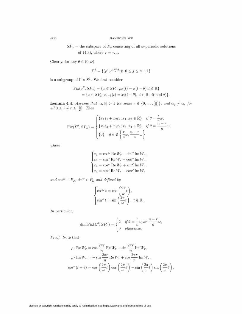
all 0 ≤ j 6= r ≤ [n2 ]. Then

Fix(Σθ, SPω) =

x1ε1 + x2ε2;x1, x2 ∈ R if θ =

r

nω,

x3ε3 + x4ε4;x3, x4 ∈ R if θ =n− r

nω,

0 if θ 6∈r

nω,n− r

nω

where

ε1 = cosω ReWr − sinω ImWr,

ε2 = sinω ReWr + cosω ImWr,

ε3 = cosω ReWr + sinω ImWr,

ε4 = sinω ReWr − cosω ImWr

and cosω ∈ Pω, sinω ∈ Pω and defined bycosω t = cos

(2πωt

),

sinω t = sin(

2πωt

), t ∈ R.

In particular,

dim Fix(Σθ, SPω) =

2 if θ =r

nω or

n− r

nω,

0 otherwise.

Proof. Note that

ρ · ReWr = cos2πrn

ReWr + sin2πrn

ImWr,

ρ · ImWr = − sin2πrn

ReWr + cos2πrn

ImWr,

cosω(t+ θ) = cos(

2πωt

)cos(

2πωθ

)− sin

(2πωt

)sin(

2πωθ

),



sinω(t+ θ) = sin(

2πωt

)cos(

2πωθ

)+ cos

(2πωt

)sin(

2πωθ

).

Consequently,

ρ · (x1ε1 + x2ε2 + x3ε3 + x4ε4)

= x1 cosω

[cos

2πrn

ReWr + sin2πrn

ImWr

]− x1 sinω

[− sin

2πrn

ReWr + cos2πrn

ImWr

]+ x2 sinω

[cos

2πrn

ReWr + sin2πrn

ImWr

]+ x2 cosω

[− sin

2πrn

ReWr + cos2πrn

ImWr

]+ x3 cosω

[cos

2πrn

ReWr + sin2πrn

ImWr

]+ x3 sinω

[− sin

2πrn

ReWr + cos2πrn

ImWr

]+ x4 sinω

[cos

2πrn

ReWr + sin2πrn

ImWr

]− x4 cosω

[− sin

2πrn

ReWr + cos2πrn

ImWr

]= x1 cos

2πrn

[cosω ReWr − sinω ImWr ]

+ x1 sin2πrn

[cosω ImWr + sinω ReWr]

+ x2 cos2πrn

[sinω ReWr + cosω ImWr]

+ x2 sin2πrn

[sinω ImWr − cosω ReWr]

+ x3 cos2πrn

[cosω ReWr + sinω ImWr]

+ x3 sin2πrn

[cosω ImWr − sinω ReWr]

+ x4 cos2πrn

[sinω ReWr − cosω ImWr]

+ x4 cos2πrn

[sinω ImWr + cosω ReWr]

=(x1 cos

2πrn

− x2 sin2πrn

)ε1 +

(x1 sin

2πrn

+ x2 cos2πrn

)ε2

+(x3 cos

2πrn

+ x4 sin2πrn

)ε3 +

(−x3 sin

2πrn

+ x4 cos2πrn

)ε4,


4822 JIANHONG WU

and

(x1ε1 + x2ε2 + x3ε3 + x4ε4)(·+ θ)

= x1

[cosω cos

2πωθ − sinω sin

2πωθ

]ReWr

− x1

[sinω cos

2πωθ + cosω sin

2πωθ

]ImWr

+ x2

[sinω cos

2πωθ + cosω sin

2πωθ

]ReWr

+ x2

[cosω cos


2πωθ

]ImWr

+ x3

[cosω cos


2πω

]ReWr

+ x3

[sinω cos

2πωθ + cosω sin

2πωθ

]ImWr

+ x4

[sinω cos

2πωθ + cosω sin

2πωθ

]ReWr

− x4

[cosω cos


2πωθ

]ImWr

= x1 cos2πωθ[cosω ReWr − sinω ImWr]

− x1 sin2πωθ[sinω ReWr + cosω ImWr]

+ x2 cos2πωθ[sinω ReWr + cosω ImWr]

+ x2 sin2πωθ[cosω ReWr − sinω ImWr]

+ x3 cos2πωθ[cosω ReWr + sinω ImWr]

+ x3 sin2πωθ[− sinω ReWr + cosω ImWr ]

+ x4 cos2πωθ[sinω ReWr − cosω ImWr]

+ x4 sin2πωθ[cosω ReWr + sinω ImWr]

=(x1 cos

2πωθ + x2 sin

2πωθ

)ε1 +

(−x1 sin

2πωθ + x2 cos

2πωθ

)ε2

+(x3 cos

2πωθ + x4 sin

2πω

)ε3 +

(−x3 sin

2πωθ + x4 cos

2πωθ

)ε4.

Consequently, in order for the following equality

ρ · (x1ε1 + x2ε2 + x3ε3 + x4ε4)

= (x1ε1 + x2ε2 + x3ε3 + x4ε4)(·+ θ)(4.5)



to hold, we must have

x1 cos2πrn

− x2 sin2πrn

= x1 cos2πrnθ + x2 sin

2πnθ

x1 sin2πrn

+ x2 cos2πrn

= −x1 sin2πnθ + x2 cos

2πωθ

x3 cos2πrn

+ x4 sin2πrn

= x3 cos2πωθ + x4 sin

2πωθ

x4 cos2πrn

− x3 sin2πrn

= x4 cos2πωθ − x3 sin

2πωθ.

Consequently, (4.5) holds if and only if

θ =n− r

nω, x3 = x4 = 0, x1, x2 ∈ R, or

θ =r

nω, x1 = x2 = 0, x3, x4 ∈ R, or

θ 6= n− r

nω,

r

nω, x1 = x2 = x3 = x4 = 0.

Clearly,

SPω = x1ε1 + x2ε2 + x3ε3 + x4ε4;x1, x2, x3, x4 ∈ R.The conclusion thus follows.

Note that

Σm = (κ, 1), (1, 1)and

Σs = (κ,−1), (1, 1)are also subgroups of Γ × S1. A similar argument to that of Lemma 4.4 leads tothe following:

Lemma 4.5. Assume that |αrβ| > 1 for some r ∈ 0, . . . , [n2 ], and αj 6= αr for

all 0 ≤ j 6= r ≤ [n2 ]. Then

Fix(Σm, SPω) =

4∑

i=1

xiεi ;x3 = x1 cos4πn− x2 sin

4πn,

x4 = x1 sin4πn

+ x2 cos4πn, x1, x2 ∈ R

and

Fix(Σs, SPω) =

4∑

i=1

xiεi ;x3 = −x1 cos4πn

+ x2 sin4πn,

x4 = − x1 sin4πn− x2 cos

4πn, x1, x2 ∈ R

.

In particular, dim Fix(Σm, SPω) = dim Fix(Σs, SPω) = 2.

Lemmas 4.2–4.5 enable us to apply Theorem 2.1 to obtain the following resulton the existence of smooth local Hopf bifurcations of wave solutions:


4824 JIANHONG WU

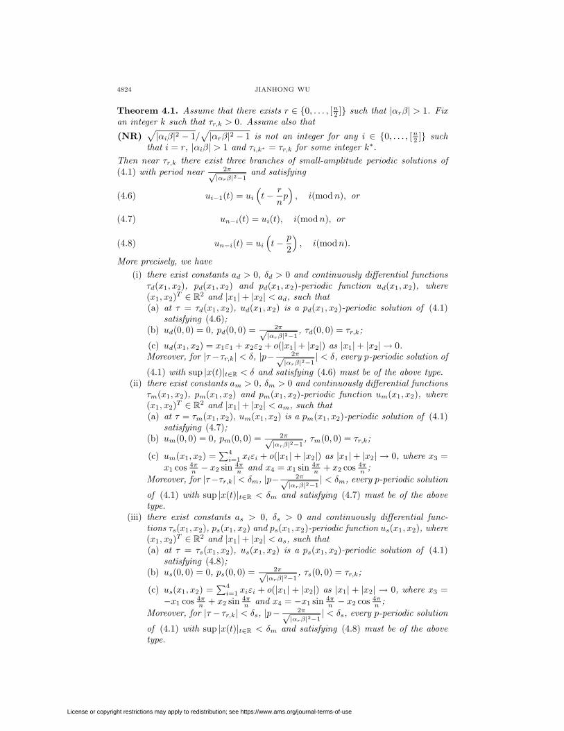
Theorem 4.1. Assume that there exists r ∈ 0, . . . , [n2 ] such that |αrβ| > 1. Fix

an integer k such that τr,k > 0. Assume also that

(NR)√|αiβ|2 − 1/

√|αrβ|2 − 1 is not an integer for any i ∈ 0, . . . , [n2 ] such

that i = r, |αiβ| > 1 and τi,k∗ = τr,k for some integer k∗.Then near τr,k there exist three branches of small-amplitude periodic solutions of(4.1) with period near 2π√

|αrβ|2−1and satisfying

ui−1(t) = ui

(t− r

np), i(modn), or(4.6)

un−i(t) = ui(t), i(modn), or(4.7)

un−i(t) = ui

(t− p

2

), i(modn).(4.8)

More precisely, we have(i) there exist constants ad > 0, δd > 0 and continuously differential functions

τd(x1, x2), pd(x1, x2) and pd(x1, x2)-periodic function ud(x1, x2), where(x1, x2)T ∈ R2 and |x1|+ |x2| < ad, such that(a) at τ = τd(x1, x2), ud(x1, x2) is a pd(x1, x2)-periodic solution of (4.1)

satisfying (4.6);(b) ud(0, 0) = 0, pd(0, 0) = 2π√

|αrβ|2−1, τd(0, 0) = τr,k;

(c) ud(x1, x2) = x1ε1 + x2ε2 + o(|x1|+ |x2|) as |x1|+ |x2| → 0.Moreover, for |τ−τr,k| < δ, |p− 2π√

|αrβ|2−1| < δ, every p-periodic solution of

(4.1) with sup |x(t)|t∈R < δ and satisfying (4.6) must be of the above type.(ii) there exist constants am > 0, δm > 0 and continuously differential functions

τm(x1, x2), pm(x1, x2) and pm(x1, x2)-periodic function um(x1, x2), where(x1, x2)T ∈ R2 and |x1|+ |x2| < am, such that(a) at τ = τm(x1, x2), um(x1, x2) is a pm(x1, x2)-periodic solution of (4.1)

satisfying (4.7);(b) um(0, 0) = 0, pm(0, 0) = 2π√

|αrβ|2−1, τm(0, 0) = τr,k;

(c) um(x1, x2) =∑4

i=1 xiεi + o(|x1|+ |x2|) as |x1|+ |x2| → 0, where x3 =x1 cos 4π

n − x2 sin 4πn and x4 = x1 sin 4π

n + x2 cos 4πn ;

Moreover, for |τ−τr,k| < δm, |p− 2π√|αrβ|2−1

| < δm, every p-periodic solution

of (4.1) with sup |x(t)|t∈R < δm and satisfying (4.7) must be of the abovetype.

(iii) there exist constants as > 0, δs > 0 and continuously differential func-tions τs(x1, x2), ps(x1, x2) and ps(x1, x2)-periodic function us(x1, x2), where(x1, x2)T ∈ R2 and |x1|+ |x2| < as, such that(a) at τ = τs(x1, x2), us(x1, x2) is a ps(x1, x2)-periodic solution of (4.1)

satisfying (4.8);(b) us(0, 0) = 0, ps(0, 0) = 2π√

|αrβ|2−1, τs(0, 0) = τr,k;

(c) us(x1, x2) =∑4

i=1 xiεi + o(|x1| + |x2|) as |x1| + |x2| → 0, where x3 =−x1 cos 4π

n + x2 sin 4πn and x4 = −x1 sin 4π

n − x2 cos 4πn ;

Moreover, for |τ − τr,k| < δs, |p− 2π√|αrβ|2−1

| < δs, every p-periodic solution

of (4.1) with sup |x(t)|t∈R < δm and satisfying (4.8) must be of the abovetype.



Remark 4.1. Periodic solutions satisfying (4.6) are called discrete waves in the lit-erature (cf. Fiedler [16] and Golubitsky, Stewart and Schaeffer [25] and referencestherein). They are also called synchronous oscillations (if r 6= 0) or phase-locked os-cillations (if r 6= 0) as each neuron oscillates just like others except not necessarily inphase with each other. The existence of synchronous oscillation in ordinary/partialdifferential equations has been extensively studied (cf. Alexander and Auchmuty[3]) and some existence results have also been obtained for functional differentialequations in conjunction with Turing rings with delayed coupling (see Krawcewiczand Wu [40] and Wu and Krawcewicz [55]. Periodic solutions satisfying (4.7) and(4.8) are called mirror-reflecting solutions and standing waves, respectively.

Remark 4.2. As will be shown in the next section, the non-resonance condition(NR) is not necessary for the existence of bifurcations of periodic solutions.

5. Applications to delayed neural networks:Global continua of discrete waves

Consider system (4.1) with a symmetric circulant interconnection matrix. Re-sults in Section 4 show that, under certain conditions, system (4.1) has branches ofperiodic solutions u(t) which satisfy the following property:

ui−1(t) = ui

(t− r

np), i(modn),(5.1)

where p is a period of u(t) and r is an integer satisfying 0 ≤ r ≤ n− 1.Let x(t) = u1(t). Clearly, if u(t) is a solution of (4.1) satisfying (5.1), the x(t) is

a solution of the following scalar functional differential equation

x(t) = −x(t) +n∑

j=1

ajf

[x

(t+

(j − 1)rn

p− τ

)].(5.2)

Conversely, if x(t) is a p-periodic solution of (5.2), then

u(t) =(x(t), x

(t+

r

np), . . . , x

(t+

(n− 1)rn

p

))T

is a p-periodic solution of (4.1) satisfying (5.1). Consequently, there exists a one-to-one correspondence between a p-periodic solution of the scalar equation (5.2)and a discrete wave satisfying (5.1) of the system (4.1).

When r = 0, system (5.2) reduces to the following scalar delay-differential equa-tion

x(t) = −x(t) +

n∑j=1

aj

f(x(t− τ)).(5.3)

This equation has been extensively studied. In particular, Mallet-Paret and Nuss-baum [45] proved the following:

Theorem 5.1. If β∑n

j=1 aj < −1, then for each

τ > τk :=1√

|∑nj=1 ajβ|2 − 1

[π − arccos

1|∑n

j−1 aj | + 2kπ

], k = 0, 1, . . . ,

equation (5.3) has at least (k+1) periodic solutions x1(t), . . . , xk+1(t) such that theperiod of x1(t) is larger than 2τ and the period of xm(t), 1 ≤ m ≤ k, is in the open


4826 JIANHONG WU

interval ( τm+ 1

2, τ

m ). Hence, for each τ > τk, (4.1) has (k + 1) distinct synchronousoscillations with periods in (2τ,∞) and ( τ

m+ 12, τ

m ), respectively.

We now follow Mallet-Paret and Nussbaum [45] and call a periodic solution of(4.1) a slowly oscillatory solution if its period is larger than twice the delay, and arapidly oscillatory solution if otherwise. So, Theorem 5.1 shows the coexistence ofa slowly oscillatory synchronous oscillation and k rapidly oscillatory synchronousoscillations for τ > τk under the assumption β

∑nj=1 aj < −1.

In the case where∑n

j=1 aj > 0, we have the following analog of Theorem 4.1.

Theorem 5.2. If β∑n

j=1 aj > 1, then for each

τ > τk :=1√

(β∑n

j=1 aj)2 − 1

[2π − arccos

1β∑n

j=1 aj+ 2kπ

], k = 0, 1, . . . ,

equation (5.3) has k+1 periodic solutions x1(t), . . . , xk+1(t) with periods in (τ, 2τ),( τ

m+1 ,τm ), 1 ≤ m ≤ k, respectively. Hence, for each τ > τk, (4.1) has k + 1

synchronous oscillation with periods in (τ, 2τ), ( τm+1 ,

τm ), 1 ≤ m ≤ k, respectively.

We defer the proof of this result to Remark 5.1.Due to the topological nature of our global bifurcation theorem, we are unable to

describe the stability of the obtained synchronous oscillation. In fact, the followingresult shows that in certain situations, the obtained synchronous oscillations are allunstable.

Theorem 5.3. If 0 ≤ ∑nj=1 aj < β−1, then the trivial solution of (5.3) is a

global attractor. Hence, (4.1) has no synchronous oscillations for all τ ≥ 0. Ifβ∑n

j=1 aj > 1, then equation (5.3) has three equilibria y∗ < 0 < z∗ such that al-most every solution of (5.3) is convergent to either y∗ or z∗. In particular, (4.1)has no stable synchronous oscillation for all τ ≥ 0.

Proof. The result is trivial if∑n

j=1 aj = 0. If∑n

j=1 aj > 0, then property (TF)implies that equation (5.3) has only one equilibrium 0 if β

∑nj=1 aj < 1, and has

three equilibria y∗ < 0 < z∗ such that f ′(y∗), f ′(z∗) < 1∑j=1 aj

if β∑n

j=1 aj > 1.The solution semiflow generated by equation (5.3) is eventually strongly monotone,and hence the stability of an equilibrium x∗ is determined by the associated ordinarydifferential equation x = −x +

∑nj=1 ajf

′(x∗)x by Theorem 3.1 of Smith [52].Consequently, if β

∑nj=1 aj < 1, then the unique equilibrium 0 is asymptotically

stable, and if β∑n

j=1 aj > 1, then the trivial solution is unstable and other equilibriay∗ and z∗ are asymptotically stable. The generic convergence to the asymptoticallystable equilibria is a consequence of the general theory of monotone dynamicalsystems developed by Hirsch [32] and Smith [52]. This completes the proof.

Throughout the remainder of this section, we assume

β

n∑j=1

aj < 1.(5.4)

It can be easily shown that under this assumption, 0 is the only equilibrium of (5.2)for all p, τ > 0. Our goal is to apply the global bifurcation theorem in Section 3to investigate the maximal continuation of each branch of discrete waves obtained



in Section 4. (The discussion of the maximal continua of standing waves andmirror-reflecting waves is similar and thus omitted). The existence results in theprevious section is local in character; the amplitude is small and the delay τ is closeto the bifurcation values τr,k. We will show that the existence of discrete waves(synchronous/phase-locked oscillations) is preserved as τ moves away form thesebifurcation values. Clearly, as τ moves away from τr,k, the amplitude of discretewaves may increase. Consequently, we obtain large-amplitude periodic solutions.

First of all, we establish some a priori bounds for possible periodic solutions of(5.2).

Lemma 5.1. If x(t) is a non-constant periodic solution of (5.2), then |x(t)| < 1for all t ∈ R.

Proof. Let t∗ ∈ R such that |x(t∗)| = sup |x(t)|t∈R. Then x(t∗) 6= 0 and ddtx

2(t∗)= 0. But |f(x(t))| < 1 for all t ∈ R and

d

dtx2(t∗) = 2x(t∗)

−x(t∗) +n∑

j=1

ajf

(x

(t∗ +

(j − 1)rn

p− τ

))< 2

−x2(t∗) + |x(t∗)|n∑

j=1

|aj |

= −2|x(t∗)||x(t∗)| − n∑

j=1

|aj |

= −2|x(t∗)|[|x(t∗)| − 1].

Consequently, |x(t∗)| < 1. This completes the proof.

Next, we exclude some periodic solutions with specific periods.

Lemma 5.2. If the diagonal elements of J are zero, then system (4.1) has nonon-constant periodic solutions of period τ . Consequently, (5.2) with p = τ has nonon-constant periodic solution of period τ .

Proof. If u(t) is a period solution of (4.1) of period τ , then u(t) solves the systemof ordinary differential equations

ui = −ui +n∑

j=1

Jijf(uj), 1 ≤ i ≤ n.(5.5)

For this system of ordinary differential equations, Hopfield [33] showed that thetime derivative of the energy function

E = −12

∑i,j

Jijf(ui)f(uj) +n∑

i=1

∫ f(ui)

0

f−1(v) dv

is

dE

dt= −

n∑i=1

f ′(ui)

ui(t)−n∑

j=1

Jijf(uj)

2

.


4828 JIANHONG WU

Therefore, by the well-known invariance principle, each solution of (5.5) is conver-gent to an equilibrium. Consequently, (5.5) (and thus (4.1)) has no non-constantperiodic solution of period τ . This completes the proof.

Lemma 5.3. Assume that there exists a positive integer s such that γsf(y)/y < 1for y 6= 0, where

γs = max

Ren∑

j=1

ajz(j−1)s−1; zns = 1

,

then equation (5.2) has no non-constant r−1nsτ-periodic solution (here, we assumer 6= 0).

Proof. Suppose that x(t) is an r−1nsτ -periodic solution of (5.2) with p = r−1nsτ .Then

x(t) = −x(t) +n∑

j=1

ajf [x(t+ (j − 1)sτ − τ)].

Clearly, x(t) is also nsτ -periodic. Let

yj(t) = x(t+ (j − 1)τ), j(modns)

y = (y1, . . . , yns)T ,

A = circ(0, . . . , 0, a2︸︷︷︸s

, 0, . . . , 0, a3︸︷︷︸s

, . . . , 0, . . . , 0, an︸︷︷︸s

, 0, . . . , 0, a1︸︷︷︸s

)

F (y) = (f(y1), . . . , f(yns))T .

Then

y = −y +AF (y).(5.6)

By Lemma 1.1 of Nussbaum [50] for the spectral analysis of circulant matrices, wehave

(−Az, z) ≥ min

Ren∑

j=1

(−aj)z(j−1)s−1; zns = 1

ns∑i=1

z2i

= −max

Ren∑

j=1

ajz(j−1)s−1; zns = 1

ns∑i=1

z2i

= −γs

ns∑i=1

z2i , z ∈ Rns.

That is,

(Az, z) ≤ γs

ns∑i=1

z2i .



Consequently, for V (y) =∑n

i=1

∫ yi

0f(s) ds, along solutions of (5.6), we have

d

dtV (y(t)) = F (y)T [−y +AF (y)]

=ns∑i=1

yif(yi) + (AF (y), F (y))

≤ −ns∑i=1

f(yi)yi

[1− γs

f(yi)yi

].

Therefore, if γsf(y)

y < 1 for all y 6= 0, then ddtV (y(t)) < 0 along nontrivial solutions

of (5.6). This implies that (5.6) has no non-constant periodic solutions. Hence,x(t) must be constant. This completes the proof.

Theorem 5.4. Assume that

(i) (5.4) is satisfied;(ii) there exists an integer r ∈ 0, . . . , [n

2 ] such that |αrβ| > 1;(iii) there exist an integer k and two nonnegative numbers qr,k,1 < qr,k,2 such

that τr,k > 0,

qr,k,1 <2π

θr − arccos 1|αrβ| + 2kπ

< qr,k,2

and (5.2) has non non-constant periodic solutions of period qr,k,1τ or qr,k,2τ .

Then for every τ > τr,k, system (4.1) has a discrete wave (a p-periodic solution)satisfying ui−1(t) = ui(t− r

np) for t ∈ R, i(modn) and qr,k,1 < p/τ < qr,k,2.

Proof. We regard (τ, p) as parameters and apply Theorem 3.3. By (5.4), we can eas-ily show that (0, τ, p) is the only stationary solution of (5.2) and the correspondingcharacteristic matrix

∆(0,τ,p)(λ) = λ+ 1−n∑

j=1

ajβeλ( j−1

n rp−τ)

is clearly continuous in (τ, p, λ) ∈ R+ × R+ × C. This justifies (A1)–(A3) of Theo-rem 3.3 for the considered equation (5.2).

To locate centers, we consider

∆(0,τ,p)

(i2mπp

)= i

2mπp

+ 1−n∑

j=1

ajβξ(j−1)rme−ir 2mπ

p

= i2mπp

+ 1− αmrβe−iτ 2mπ

p

= q

(i2mπp

),

where

q(λ) = λ+ 1− amrβe−τλ.

Using results in Lemma 4.1 and notations in Lemma 4.2, we can show that for eachfixed r, (0, τ, p) is a center if and only if there exist an integer m ≥ 1 and an integer


4830 JIANHONG WU

k such that |αmrβ| > 1,p = 2mπ√

|αmrβ|2−1,

τ = τmr,k > 0.

In particular, (0, τr,k, 2π√|αrβ|2−1

) is a center and all centers are isolated. In fact,

the set of centers is countable and can be expressed as

∆ =

(0, τmr,k,

2mπ√|αmrβ|2 − 1

); |αmrβ| > 1, τmr,k > 0

.

We now fix r ∈ 0, . . . , n− 1 such that |αrβ| > 1. Then (0, τr,k, 2π√|αrβ|2−1

) is an

isolated center and 1 ∈ J(0, τ∗r ,2π√

|αrβ|2−1).

Consider q(λ) with m = 1. By Lemma 4.1 there exist ε > 0, δ > 0 and a smoothcurve λ : (τr,k − δ, τr,k + δ) → C such that q(λ(τ)) = 0, |λ(τ) − i 2π√

|αrβ|2−1| < ε for

all τ ∈ [τr,k − δ, τr,k + δ], and

λ(τr,k) = i2π√|αrβ|2 − 1

,d

dτReλ(τ)|τ=τr,k

> 0.

Let

Ωε =

(0, p); 0 < u < ε,

∣∣∣∣∣p− 2π√|αrβ|2 − 1

∣∣∣∣∣ < ε

.

Clearly, if |τ − τr,k| ≤ δ and (u, p) ∈ ∂Ωε such that det∆(0,τ,p)(u + i 2πp ) = 0, then

τ = τr,k, u = 0 and p = 2π√|αrβ|2−1

. This justifies (A4) for m = 1. Moreover, if we

put

H±m

(0, τr,k,

2π√|αrβ|2 − 1

)(u, p) = ∆(0,τr,k±δ,p)

(u+ im

2πp

),

then at m = 1, we have

γm

(0, τr,k,

2π√|αrβ|2 − 1

)

= degB

(H−

m

(0, τr,k,

2π√|αrβ|2 − 1

),Ωε

)

− degB

(H+

m

(0, τr,k,

2π√|αrβ|2 − 1

),Ωε

)= −1.

By Theorem 3.3, we conclude that the connected component C(0, τr,k, 2π√|αrβ|2−1

)

through (0, τr,k, 2π√|αrβ|2−1

) in Σr is nonempty, where

Σr = cl(x, τ, p); x is a p-periodic solution of (5.2).



Using the same argument as above, we can show that the first crossing number ofeach center is always −1. Therefore, we can use (3.2) to exclude alternative (ii) ofTheorem 3.3. That is, we can conclude that C(0, τr,k, 2π√

|αrβ|2−1) is unbounded.

Lemma 5.1 implies that the projection of C(0, τr,k, 2π√|αrβ|2−1

) onto the x-space

is bounded. Also, note that the proof of Lemma 5.2 implies that the system(4.1) with τ = 0 has no non-constant periodic solution. Therefore, the projec-tion of C(0, τr,k, 2π√

|αrβ|2−1) onto the τ -space is bounded below. Assumption (iii)

implies that, if (x, τ, p) ∈ C(0, τr,k, 2π√|αrβ|2−1

), then τqr,k,1 < p < τqr,q,2. This

shows that in order for C(0, τr,k, 2π√|αrβ|2−1

) to be unbounded, the projection of

C(0, τr,k, 2π√|αrβ|2−1

) onto τ -space must be unbounded. Consequently, the projection

of C(0, τr,k, 2π√|αrβ|2−1

) onto τ -space must be an interval [α,∞) with 0 < α < τr,k.

This shows that for each τ > τr,k, (5.2) has a non-constant periodic solution witha period in (τqr,k,1, τqr,k,2). This completes the proof.

Remark 5.1. We can now give a proof of Theorem 5.2. In fact, Chow and Mallet-Paret [8] have proved that equation (5.3) has no non-constant periodic solutionof period 2τ . Consequently, it has no non-constant periodic solution of period τ

m

or 2τm+1 = τ

m+ 12

for all positive integers m. Therefore, Theorem 5.2 becomes a

special case of Theorem 5.4 where r = 0, αr =∑n

j=1 aj; θr = 0, τr,k = τk−1,qr,k+1,1 = 1

k+1 , qr,k+1,2 = 1k for all k = 1, 2, . . . , and qr,1,1 = 1, qr,1,2 = 2.

Remark 5.2. We can always take q1,k,1 = 0 if we do not need good estimation of thelower bound of the period of periodic solutions. Moreover, we can use Lemma 5.2and Lemma 5.3 to determine qr,k,1 and qr,k,2 in some concrete neural networks, seethe next section for details.

Remark 5.3. Applying Theorem 3.2 and employing the same argument as that forTheorem 5.4, we can obtain a local bifurcation theorem for (4.1): If there exist r ∈0, . . . , [n

2 ] and an integer k such that |αrβ| > 1 and τr,k > 0, then near τr,k, (4.1)has a branch of small-amplitude p-periodic solution satisfying ui−1(t) = ui(t− 1

np),i(modn), t ∈ R. Note that we do not require non-resonance condition, but wecannot describe the smoothness, the isotropy group and the asymptotic form of thebifurcated wave solution.

6. Examples and further discussions

In this section, we concentrate on some specific networks to discuss some im-plications and limitations of our general results. For simplicity, we will only con-sider synchronous/phase-locked oscillations and omit the discussion about standingwaves and mirror-reflecting waves.

6.A. All-Excitatory Networks. For this special network, as f is an increasingfunction and the interconnection matrix has positive off diagonal elements, thesolution semiflow is eventually strongly monotone and hence the convergence toequilibria is the dominant dynamics. More precisely, we have

Theorem 6.1. Consider equation (4.1) with the interconnection matrix JE.


4832 JIANHONG WU

(i) If β = f ′(0) < 1, then for any τ > 0 the unique equilibrium (0, . . . , 0) isa global attractor. That is, any solution of (4.1) converges to (0, . . . , 0) ast→∞.

(ii) If β = f ′(0) > 1, then equation (4.1) has three and only three equilibria(y∗, . . . , y∗), (0, . . . , 0) and (z∗, . . . , z∗) with y∗ < 0 < z∗, f(y∗) = y∗,f(z∗) = z∗. (0, . . . , 0) is unstable, (y∗, . . . , y∗) and (z∗, . . . , z∗) are asymp-totically stable and almost every solution of (4.1) is convergent to either(y∗, . . . , y∗) or (z∗, . . . , z∗) as t→∞. Moreover, there exists a solution u(t)of (4.1) such that ui(t) < ui(s) if t < s, 1 ≤ i ≤ n, and limt→−∞ ui(t) = 0,limt→∞ ui(t) = z∗; and there exists a solution v(t) of (4.1) such thatvi(t) < vi(s) if t > s, 1 ≤ i ≤ n, and limt→−∞ vi(t) = 0, limt→∞ vi(t) = y∗.

Proof. Let (x1, . . . , xn) be an equilibrium of (4.1). Then

xi =1

n− 1

∑j 6=i

f(xj), 1 ≤ i ≤ n.

Hence,

xi − xj =1

n− 1[f(xj)− f(xi)]

and from the increasing property of f it follows that xi = xj for all 1 ≤ i, j ≤ n.Therefore, (x1, . . . , xn) is an equilibrium of (4.1) if and only if x = f(x) and xi = xfor all 1 ≤ i ≤ n. Consequently, using property (TF) we conclude that (4.1)has a unique equilibrium (0, . . . , 0) if β < 1, and has three equilibria (y∗, . . . , y∗),(0, . . . , 0), (z∗, . . . , z∗) when f(y∗) = y∗ < 0 < z∗ = f(z∗) if β > 1. In the lattercase, we also have f ′(y∗), f ′(z∗) < 1.

We now consider the case where β < 1. As f is strictly increasing and JE

has positive off diagonal elements, the general theory of Smith [52] shows that thesolution semiflow generated by (4.1) is eventually strongly monotone and the zerosolution (0, . . . , 0) of (4.1) is asymptotically stable if and only if the zero solutionof the associated ordinary differential equation

xi = −xi +∑j 6=i

β

n− 1f(xj)(6.1)

is asymptotically stable. It can be easily shown that eigenvalues of (6.1) at thetrivial solution are −1 + βαr, 0 ≤ r ≤ n− 1, where

αr =

1 if r = 0,

− 1n− 1

if 1 ≤ r ≤ n− 1.

Consequently, β < 1 implies that the zero solution of (6.1) is asymptotically stable.As each solution of (4.1) is clearly bounded, (0, . . . , 0) is the only equilibrium andis asymptotically stable. By results in Smith [52], the zero solution is a globalattractor.

In the case where β > 1, using the same argument as above we can verify that thezero solution (0, . . . , 0) is unstable, and (y∗, . . . , y∗), (z∗, . . . , z∗) are asymptoticallystable. Again, by results in Hirsch [32] and Smith [52], almost every solution of(4.1) is convergent to either (y∗, . . . , y∗) or (z∗, . . . , z∗), and there are monotonicallyheteroclinic orbits connecting (0, . . . , 0) to (y∗, . . . , y∗) and to (z∗, . . . , z∗). Thiscompletes the proof.



Remark 6.1. The above result shows that the generic dynamics of (4.1) is the con-vergence to equilibria. This is independent of the length of the delay τ . The onlyinteresting phenomena is the bifurcation of the pitchfork type: as the neuron gainmoves through value 1, the zero solution becomes unstable, and two asymptoticstable equilibria appear in either side of the origin in the ferromagnetic direction(ui = 1 for all 1 ≤ i ≤ n). This phenomena was observed in Marcus and Westervelt[47].

Let us now try to apply Theorem 5.4 and Remark 5.3 to discuss the occurrenceof discrete waves. Clearly,

αr =1

n− 1[ξr + ξ2r + · · ·+ ξ(n−1)r]

=

1 if r = 0,

− 1n− 1

if 1 ≤ r ≤ n− 1.

Let

τ0,k =1√β2 − 1

[2kπ − arccos

1β

]if β > 1 and k ≥ 1;

τk =n− 1√

β2 − (n− 1)2

[π − arccos

n− 1β

+ 2kπ]

if β > n− 1 and k ≥ 0.

Applying Remark 5.3, we get

Theorem 6.2. Consider equation (4.1) with the interconnection matrix JE.(i) If β > 1, then near τ0,k, k ≥ 1, there exists a branch of small-amplitude

synchronous oscillations, i.e. a branch of small-amplitude periodic solutionwith period near 2π/

√β2 − 1 and satisfying ui(t) = u1(t) for 1 ≤ i ≤ n and

τ ∈ R;(ii) If β > n − 1, then near τk, k ≥ 0, there exist (n − 1) branches of small-

amplitude phase-locked oscillations with distinct phase differences, i.e. (n−1) branches of small-amplitude phase-locked oscillations with period near2π(n − 1)/

√β2 − (n− 1)2 and satisfying ui−1(t) = ui(t − r

np) for t ∈ R,i(modn), 1 ≤ r ≤ n− 1.

Remark 6.2. By Theorem 6.1, any synchronous/phase-locked oscillation obtainedabove must be unstable. Consequently, in all-excitatory networks, delay may causediscrete waves but these waves can hardly be observed in experiments. An in-teresting phenomena here is the simultaneous occurrence of (n − 1) branches ofphase-locked oscillations with distinct phase differences. We should also mentionthat if (n− 1)

√β2−1

β2−(n−1)2 is not a positive integer, then we can apply Theorem 2.1to discuss the smoothness and directions of these (n− 1) branches of phase-lockedoscillations.

6.B. Rings of Inhibitory Neurons. We next consider symmetrically connectedinhibitory rings of neurons, where

αr = −12[ξr + ξ(n−1)r]

=

−1 if r = 0,− cos 2πr

n if r = 1, . . . , n− 1.


4834 JIANHONG WU

Consequently, αi = αj if and only if i+ j = n.Note that

γs = max

Re(−1

2zs−1 − 1

2z(n−1)s−1

); zns = 1

= max

−1

2Re(zs−1 + z−s−1); zns = 1

= max

−1

2

[cos

2πj(s− 1)ns

+ cos2πj(s+ 1)

ns

]; 0 ≤ j ≤ ns− 1

= max

− cos

2πjns

cos2πjn

; 0 ≤ j ≤ ns− 1.

In particular,

γ1 = max

−(

cos2πjn

)2

; 0 ≤ j ≤ n− 1

≤ 0.

Therefore,

γ1f(y)/y ≤ 0 < 1 for all y 6= 0.

Let

τ0,k =1√β2 − 1

[π − arccos

1β

+ 2kπ], if β > 1, k ≥ 0,

and

τr,k =1√

|β cos 2πrn |2 − 1

[2(k + 1)π − arccos

1|β cos 2πr

n |]

if β cos2πrn

< −1, k ≥ 0,[π − arccos

1|β cos 2πr

n | + 2kπ]

if β cos2πrn

> 1, k ≥ 0.

Theorem 6.3. Consider system (4.1) with the interconnection matrix JIE.(i) If β > 1, then for each τ > τ0,k, (4.1) has (k + 1) distinct synchronous

oscillations with periods in (2τ,∞) and ( τm+ 1

2, τ

m ), 1 ≤ m ≤ k, respectively;

(ii) If rn ∈ (1

4 ,34 ) and β cos 2πτ

n < −1, then for each τ > τrk,k, (4.1) has (k + 1)phase-locked oscillations with periods in (τ, n

r τ) and ( τm+1 ,

τm ), 1 ≤ m ≤ k,

respectively and satisfying ui−1(t) = ui(t− rnp), i(modn), t ∈ R;

(iii) If rn ∈ (0, 1

4 ) ∪ (34 , 1) and β cos 2πr

n > 1, then for each τ > τr,k, (4.1) has(k + 1) phase-locked oscillations with periods in (2τ, n

r τ) (if rn ∈ (0, 1

4 )) or(2τ, n

n−r τ) (if rn ∈ (3

4 , 1)), and ( τm+1 ,

τm ), 1 ≤ m ≤ k, respectively and

satisfying ui−1(t) = ui(t− rnp), i(modn), t ∈ R.

Proof. (i) is an immediate consequence of Theorem 5.1, where∑n

j=1 aj = −1 < 0.(ii) Assume r

n ∈ (14 ,

34 ) and β cos 2πr

n < −1. Note that

1k + 1

=2π

2(k + 1)π<

2π2(k + 1)π − arccos 1

|β cos 2πrn |

<2π

2(k + 1)π − π2

=1

k + 34

.



So,

1 <2π

2(k + 1)π − arccos 1|β cos 2πr

n |<

43<n

r, if k = 0,

1k + 1

<2π

2(k + 1)π − arccos 1|β cos 2πr

n |<

1k, if k ≥ 1.

Since γ1 ≤ 0, by Lemma 5.3, equation (5.2) has no non-constant nr τ -periodic so-

lution. Moreover, by Lemma 5.2, equation (5.2) has no non-constant τm -periodic

solution for any positive integer m. Therefore, we can apply Theorem 5.4 to obtainthe required result, where

qr,0,1 = 1, qr,0,2 =n

r, qr,k,1 =

1k + 1

, qr,k,2 =1k, k ≥ 1.

This proves (ii), and (iii) can be justified similarly.

Remark 6.3. Note that cos 2πrn = cos 2π(n−r)

n . So, τr,k = τn−r,k for all r ∈ 1, . . . ,n − 1 and k ≥ 0. Therefore, if r 6= n

2 , then at each τr,k there are two branchesof phase-locked oscillations which are conjugate in the sense that if solutions alongone branch satisfy ui−1(t) = ui(t− r

np), then solutions along another branch satisfyui−1(t) = ui(t+ r

np) (as ui(t− n−rn p) = ui(t+ r

np)). This implies that Theorem 5.3actually guarantees the existence of 2(k+1) phase-locked oscillations in either case(ii) or case (iii).

Remark 6.4. If n = 4q + m for some nonnegative integer q and integer m ∈0, 1, 2, 3, then r

n ∈ (0, 14 ) ∪ (3

4 , 1) if and only if

r ∈

1, 2, . . . , q, n− 1, . . . , n− q) if m 6= 0,∅ if m = 0 and q ≤ 1,1, . . . , q − 1, n− 1, . . . , n− q + 1 if m = 0 and q ≥ 2.

Consequently, if

β > maxrn∈(0, 1

4 )∪( 34 ,1)

1cos 2πr

n

,

then for sufficiently large τ satisfying

τ >

maxτ0,0, τ1,0, . . . , τq,0 if m 6= 0,maxτ0,0, τ1,0, . . . , τq−1,0 if q ≥ 2, m = 0,τ0,0 if m = 0, q ≤ 1,

system (4.1) has at least (2q∗+1) slowly oscillatory periodic solutions, one of whichis synchronous oscillation and others are phase-locked oscillations, where

q∗ =

q if m 6= 0,q − 1 if m = 0, q ≥ 2,0 if m− 0, 0 ≤ q ≤ 1.

6.C. All-inhibitory networks and rings of excitatory neurons. Using thesame argument as that in 6.A and 6.B, we can show that all-inhibitory networksexhibit the coexistence of synchronous and phase-locked oscillations for large delayand neural gains. It is also possible for a ring of excitatory neurons to possess


4836 JIANHONG WU

synchronous/phase-locked oscillations, but these oscillations are all unstable andthe dominant dynamics is the convergence to equilibria.

Acknowledgement

This research was supported by Natural Sciences and Engineering ResearchCouncil of Canada and by Faculty of Arts Research Grants of York University.Part of the results was reported in various meetings including Workshop on Geo-metric Methods in Ordinary Differential Equations, Oberwolfach, March of 1995;Geometric Dynamics and Its Applications, Berkeley, October of 1993; The 2nd In-ternational Conference on Differential Equations, Athens, August of 1993; SIAMConference on Applications of Dynamical Systems, Snowbird, October of 1992. Theauthor has benefited very much from discussions with and encouragement from J.Belair, B. Fiedler, A. Herz, M. Hirsch, J. Mallet-Paret, J. Mawhin, K. Mischaikow,R. Nussbaum, K. Schmidt, P. van den Driessche and H. O. Walther.

References

[1] J. C. Alexander, Bifurcation of zeros of parametrized functions, J. Funct. Anal. 29 (1978),37–53. MR 80j:58023

[2] J. C. Alexander and G. Auchmuty, Global branching of waves, Manuscripta Math. 27 (1979),159–166. MR 80g:58021

[3] , Global bifurcations of phase-locked oscillators, Arch. Rational Mech. Anal. 93 (1986),253–270. MR 87j:34090

[4] J. C. Alexander and P. M. Fitzpatrick, The homotopy of certain spaces of nonlinear operators,and its relation to global bifurcation of the fixed points of parametrized condensing operators,J. Funct. Anal. 34 (1979), 87–106. MR 81k:58023

[5] J. C. Alexander and J. Yorke, Global bifurcation of periodic orbits, Amer. J. Math. 100(1978), 263–292. MR 57:14046

[6] J. Belair, Stability in a model of a delayed neural network, J. Dynamics and DifferentialEquations 5 (1993), 607–623. MR 94i:34150

[7] R. D. Braddock and P. van den Driessche, On the stability of differential-difference equations,J. Austral. Math. Soc. 19(B) (1976), 358–370. MR 56:6058

[8] S. N. Chow and J. Mallet-Paret, The fuller index and global Hopf bifurcation, J. DifferentialEquations 29 (1978), 66–85. MR 58:11665

[9] S. N. Chow, J. Mallet-Paret and J. A. Yorke, Global Hopf bifurcation from a multiple eigen-value, Nonlinear Anal. 2 (1978), 753–763. MR 80a:58015

[10] M. A. Cohn and S. Grossberg, Absolute stability of global pattern formation and parallelmemory storage by competitive neural networks, IEEE Trans. Systems Man Cybernet. 13(1983), 815–826. MR 85e:92002

[11] E. N. Dancer, Boundary-value problems for ordinary differential equations on infinite inter-vals, Proc. London Math. Soc. 30 (1975), 76–94. MR 52:867

[12] G. Dylawerski, K. Geba, J. Jodel and W. Marzantowicz, S1-equivalent degree and the Fullerindex, Ann. Polon. Math. 52 (1991), 243–280. MR 92g:58105

[13] L. H. Erge, K. Geba, W. Krawcewicz, and J. Wu, S1-degree and global Hopf bifurcationtheory of functional differential equations, J. Differential Equations 98 (1992), 277–298. MR93f:58034

[14] C. Fenske, Analytische Theorie des Abbildungrades fur Abbildungen in Banachraumes, Math.Nachr. 48 (1971), 279–290. MR 49:7857

[15] B. Fiedler, An index for global Hopf bifurcation in parabolic systems, J. Reine Angew. Math.359 (1985), 1–36. MR 87c:58024

[16] , Global Bifurcation of Periodic Solutions with Symmetry, Lecture Notes in Math.,Vol. 1309, Springer-Verlag, New York, 1988. MR 90c:58125

[17] P. M. Fitzpatrick, Homotopy, linearization, and bifurcation, Nonlinear Anal. 12 (1988), 171–184. MR 89g:58039

[18] A. Frumkin and E. Moses, Physicality of the Little model, Physical Review (A), 34 (1986),714–716.



[19] F. B. Fuller, An index of fixed point type for periodic orbits, Amer. J. Math. 89 (1967),133–148. MR 35:497

[20] K. Geba, W. Krawcewicz and J. Wu, An equivariant degree with applications to symmetricbifurcation problems, I: construction of the degree, Proc. London Math. Soc. 69 (1994), 377–398. MR 95g:58025

[21] K. Geba an W.. Marzantowicz, Global bifurcation of periodic solutions, Topological Methodsin Nonlinear Analysis 1 (1993), 67–93. MR 94e:58024

[22] E. Goles-Chacc, F. Fogelman-Soulie and D. Pellegrin, Decreasing energy functions as a toolfor studying threshold networks, Discrete Appl. Math. 12 (1985), 261–277. MR 87d:68084

[23] E. Goles and G. Y. Vichniac, Lyapunov functions for parallel neural networks, in “NeuralNetworks for Computing (J. S. Denber ed.)”, Amer. Inst. Phy., New York (1986), pp. 165–181.

[24] M. Golubitsky and I. N. Stewart, Hopf bifurcation in the presence of symmetry, Arch. Ra-tional Mech. Anal. 87 (1985), 107–165. MR 86g:58034

[25] M. Golubitsky, I. Stewart and D. G. Schaeffer, Singularities and Groups in Bifurcation The-

ory, Vol. 2, Springer-Verlag, New York, 1988. MR 89m:58038[26] G. Grinstein, C. Jayaprakash and P. He, Statistical mechanics of probabilistic automata,

Phys. Rev. Lett. 55 (1985), 2527–2530. MR 87c:82029[27] J. Hale, Theory of Functional Differential Equations, Springer-Verlag, New York 1977. MR

58:22904[28] , Nonlinear Oscillations in Equations with Delays, in “Nonlinear Oscillations in Biol-

ogy”, pp. 157–185, Lectures in Applied Mathematics, Vol. 17, Amer. Math. Soc., Providence,RI, 1979. MR 81d:34062

[29] D. Hassard, N. D. Kazarinoff and Y. Wan, Theory and Applications of Hopf Bifurcation,Cambridge Univ. Press, Cambridge, 1981. MR 82j:58089

[30] A. Herz, B. Salzer, R. Kuhn and J. L. van Hemmen, Hebbian learning reconsidered: repre-sentation of static and dynamic objects in associative neural nets, Biol. Cybern. 60 (1989),457–467.

[31] G. Hetzer and V. Stallbohm, Global behaviour of bifurcation branches and the essentialspectrum, Math. Nachr. 86 (1978), 343–360. MR 80g:47076

[32] M. W. Hirsch, Stability and convergence in strongly monotone dynamical systems, J. ReineAngew. Math. 383 (1988), 1–53. MR 89c:58108

[33] J. J. Hopfield, Neural networks and physical systems with emergent collective computationalabilities, Proc. Nat. Acad. Sci. 79 (1982), 2554–2558. MR 83g:92024

[34] J. J. Hopfield, Neurons with graded response have collective computational properties likethose of two-stage neurons, Proc. Nat. Acad. Sci. 81 (1984), 3088–3092.

[35] J. Ize, Bifurcation theory for Fredholm operators, Mem. Amer. Math. Soc. 17 (1976). MR54:13649

[36] , Obstruction theory and multiparameter Hopf bifurcation, Trans. Amer. Math. Soc.209 (1985), 757–792.

[37] J. Ize, I. Massabo and A. Vignoli, Degree theory for equivariant maps, (I). Trans. Amer.Math. Soc. 315 (1989), 433–510. MR 90a:58030

[38] , Degree theory for equivariant maps, (II). The general S1-action, Mem. Amer. Math.100 (1992). MR 93d:58030

[39] W. Krawcewicz, P. Vivi and J. Wu, Computation formulae of an equivalent degree withapplications to symmetric bifurcations, Nonlinear Studies 4 (1997), 89–120. CMP 97:14

[40] W. Krawcewicz and J. Wu, Theory and applications of Hopf bifurcations in symmetric func-tional differential equations, Nonlinear Analysis, in press.

[41] W. Krawcewicz, H. Xia and J. Wu, Global bifurcation theory for condensing fields and neu-tral equations with applications to lossless transmission problems, Canadian Appl. Math.Quarterly 1 (1993), 167–220. MR 94g:47077

[42] B. W. Levinger, A folk theorem in functional differential equations, J. Differential Equations4 (1980), 612–619. MR 37:6566

[43] W. A. Little, Existence of persistent states in the brain, Math. Biosci. 19 (1974), 101–120.[44] W. A. Little and G. L. Shaw, Analytic study of the memory storage capacity of a neural

network, Math. Biosci. 39 (1978), 281–290.[45] J. Mallet-Paret and R. D. Nussbaum, Global continuation and asymptotic behaviour for

periodic solutions of a differential-delay equation, Ann. Mate. Pura. Appl. 145 (1986), 33–128. MR 88e:34127


4838 JIANHONG WU

[46] J. Mallet-Paret and J. Yorke, Snakes: oriented families of periodic orbits, their sources, sinksand continuation, J. Differential Equations 43 (1992), 419–450. MR 84a:58071

[47] C. M. Marcus and R. M. Westervelt, Stability of analog neural networks with delay, PhysicalReview A 39 (1989), 347–359. MR 89m:92025

[48] R. D. Nussbaum, A global bifurcation theorem with applications to functional differentialequations, J. Funct. Anal. 19 (1975), 319–338. MR 52:6516

[49] , A Hopf global bifurcation theorem for retarded functional differential equations,Trans. Amer. Math. Soc. 238 (1978), 139–164. MR 81h:34082

[50] , Circulant matrices and differential-delay equations, J. Differential Equations 60(1985), 201–217. MR 87d:34112

[51] P. H. Rabinowitz, Some global results for nonlinear eigenvalue problems, J. Functional Anal.7 (1971), 487–513. MR 46:745

[52] H. L. Smith, Monotone semiflows generated by functional differential equations, J. Differen-tial Equations 66 (1987), 420—442. MR 88j:34155

[53] C. A. Stuart, Some bifurcation theory for k-set contractions, Proc. London Math. Soc. 27(1973), 531–550. MR 48:12178

[54] A. Vanderbauwhede, Local Bifurcation and Symmetry, Res. Notes Math., 75, Pitman, Boston,1982. MR 85f:58026

[55] J. Wu and W. Krawcewicz, Discrete waves and phase-locked oscillations in the growth of asingle-species population over a patchy environment, Open Systems and Information Dynam-ics 1 (1992), 127–147.

Department of Mathematics and Statistics, York University, North York, Ontario,Canada M3J 1P3

E-mail address: [email protected]


Documents

SYMMETRIC FUNCTIONAL DIFFERENTIAL EQUATIONS AND …SYMMETRIC FUNCTIONAL DIFFERENTIAL EQUATIONS AND NEURAL NETWORKS WITH MEMORY JIANHONG WU ... for systems of functional di erential