Symbolic Computation of Lax Pairsof Systems of Partial Difference Equations

Using Consistency Around the Cube

Willy Hereman & Terry BridgmanDepartment of Applied Mathematics and Statistics

Colorado School of Mines

Golden, Colorado, U.S.A.

http://www.mines.edu/fs home/whereman/

AMS Spring Western Sectional Meeting

University of Colorado, Boulder

Saturday, April 13, 2013, 3:00p.m.

Collaborators

Reinout Quispel & Peter van der Kamp

La Trobe University, Melbourne, Australia

Paper to appear:

Bridgman, Hereman, Quispel, van der Kamp

Foundations of Computational

Mathematics, 13, 3 or 4? (2013)

Research supported in part by NSF

under Grant CCF-0830783

This presentation is made in TeXpower

Outline

• What are nonlinear P∆Es?

• Lax pairs in matrix form of nonlinear PDEs

• Lax pair of nonlinear P∆Es

• Algorithm to compute Lax pairs of P∆Es

(Nijhoff 2001, Bobenko & Suris 2001)

• Additional examples

• Conclusions and future work

What are nonlinear P∆Es?

• Nonlinear maps with two (or more) lattice points

Some origins:

I full discretizations of PDEs

I discrete dynamical systems in 2 dimensions

I superposition principle (Bianchi permutability)

for Backlund transformations between 3

solutions (2 parameters) of a completely

integrable PDE

• Example 1: discrete potential Korteweg-de

Vries (pKdV) equation

(un,m − un+1,m+1)(un+1,m − un,m+1)− p2 + q2 = 0

• u is dependent variable or field (scalar case)

n and m are lattice points

p and q are parameters

• Notation:

(un,m, un+1,m, un,m+1, un+1,m+1) = (x, x1, x2, x12)

• Alternate notations (in the literature):

(un,m, un+1,m, un,m+1, un+1,m+1) = (u, u, u, ˆu)

(un,m, un+1,m, un,m+1, un+1,m+1) = (u00, u10, u01, u11)

• Example 1: discrete pKdV equation

(un,m − un+1,m+1)(un+1,m − un,m+1)− p2 + q2 = 0

Short: (x− x12)(x1 − x2)− p2 + q2 = 0

(un,m − un+1,m+1)(un+1,m − un,m+1)− p2 + q2 = 0

Short: (x− x12)(x1 − x2)− p2 + q2 = 0

x = un,m x1 = un+1,m

x12 = un+1,m+1x2 = un,m+1 p

p

q q

Systems of P∆Es

Example 2: Schwarzian-Boussinesq System

z1 y − x1 + x = 0

z2 y − x2 + x = 0

z y12(y1 − y2)− y(p y2 z1 − q y1 z2) = 0

• Note: System has two single-edge equations and

one full-face equation.

Concept of Consistency Around the Cube

Superposition of Backlund transformations between

4 solutions x, x1, x2, x3 (3 parameters: p, q, k)

x

x123

x12

x13

x23

x1

x2

x3

p

qk

• Introduce a third lattice variable `

• View u as dependent on three lattice points:

n,m, `. So, x = un,m −→ x = un,m,`

• Move in three directions:

n→ n+ 1 over distance p

m→ m+ 1 over distance q

`→ `+ 1 over distance k (spectral parameter)

• Require that the same lattice holds on the front,

bottom, and left faces of the cube

• Require consistency for the computation of

x123 = un+1,m+1,`+1 (3 ways → same answer)

x

x123

x12

x13

x23

x1

x2

x3

p

qk

Peter D. Lax (1926-)

Seminal paper: Integrals of nonlinear equations of

evolution and solitary waves, Commun. Pure Appl.

Math. 21 (1968) 467-490

Refresher: Lax Pairs of Nonlinear PDEs

• Historical example: Korteweg-de Vries equation

ut + αuux + uxxx = 0 α ∈ IR

• Key idea: Replace the nonlinear PDE with a

compatible linear system (Lax pair):

ψxx +(

16αu− λ

)ψ = 0

ψt + 4ψxxx + αuψx + 12αuxψ = 0

ψ is eigenfunction; λ is constant eigenvalue

(λt = 0) (isospectral)

Lax Pairs in Matrix Form (AKNS Scheme)

• Write

ψxx +(

16αu− λ

)ψ = 0

ψt + 4ψxxx + αuψx + 12αuxψ = 0

as a first-order system.

• Introduce, Ψ =

ψψx

, then, DxΨ = XΨ with

X =

0 1

λ− 16αu 0

• Use φt = ψxt = ψtx and eliminate ψx, ψxx, ψxxx, . . .

to get DtΨ = TΨ with

T =

16αux −4λ− 1

3αu

−4λ2 + 13αλu+ 1

18α2u2 + 1

6αu2x −1

6αux

• Compatibility of

DxΨ = X Ψ

DtΨ = T Ψ

yields Lax equation (zero-curvature equation):

DtX−DxT + [X,T] = 0

with commutator [X,T] = XT−TX

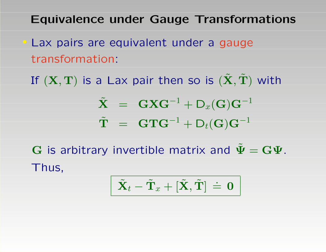
Equivalence under Gauge Transformations

• Lax pairs are equivalent under a gauge

transformation:

If (X,T) is a Lax pair then so is (X, T) with

X = GXG−1 + Dx(G)G−1

T = GTG−1 + Dt(G)G−1

G is arbitrary invertible matrix and Ψ = GΨ.

Thus,

Xt − Tx + [X, T] = 0

• Example: For the KdV equation

X =

0 1

λ− 16αu 0

and X =

−ik 16αu

−1 ik

Here,

X = GXG−1 and T = GTG−1

with

G =

−i k 1

−1 0

where λ = −k2

Reasons to Compute a Lax Pair

• Compatible linear system is the starting point for

application of the IST and the Riemann-Hilbert

method for boundary value problems

• Confirm the complete integrability of the PDE

• Zero-curvature representation of the PDE

• Compute conservation laws of the PDE

• Discover families of completely integrable PDEs

Question: How to find a Lax pair of a completely

integrable PDE?

Answer: There is no completely systematic method

Lax Pair of Nonlinear P∆Es

• Replace the nonlinear P∆E by

ψ1 = Lψ (recall ψ1 = ψn+1,m)

ψ2 = Mψ (recall ψ2 = ψn,m+1)

For scalar P∆Es, L,M are 2× 2 matrices; ψ=

fg

• Express compatibility:

ψ12 = L2 ψ2 = L2 Mψ

ψ12 = M1 ψ1 = M1 Lψ

• Lax equation: L2 M−M1 L = 0

Equivalence under Gauge Transformations

• Lax pairs are equivalent under a gauge

transformation

If (L,M) is a Lax pair then so is (L,M) with

L = G1 L G−1

M = G2 M G−1

where G is non-singular matrix and φ = Gψ

Proof: Trivial verification that

(L2M−M1 L)φ = 0↔ (L2 M−M1 L)ψ = 0

• Example 1: Discrete pKdV Equation

(x− x12)(x1 − x2)− p2 + q2 = 0

• Lax pair:

L = tLc = t

x p2 − k2 − xx1

1 −x1

M = sMc = s

x q2 − k2 − xx2

1 −x2

with t = s = 1 or t = 1√

DetLc= 1√

k2−p2

and s = 1√DetMc

= 1√k2−q2

. Here, t2t

ss1

= 1.

• Example 2: Schwarzian-Boussinesq System

z1 y − x1 + x = 0

z2 y − x2 + x = 0

z y12(y1 − y2)− y(p y2 z1 − q y1 z2) = 0

• Lax pair:

L = tLc = t

−y 0 yz1

kyy1z−pyz1

z0

0 1 −y1

M = sMc = s

−y 0 yz2

kyy2z− qyz2

z0

0 1 −y2

with t = s = 1

y, or t = 1

y1and s = 1

y2,

or t = 3

√z

y2y1z1and s = 3

√z

y2y2z2.

Here, t2t

ss1

= y1y2.

Lax Pair Algorithm for Scalar P∆Es

(Nijhoff 2001, Bobenko and Suris 2001)

Applies to P∆Es that are consistent around the cube

Example 1: Discrete pKdV Equation

• Step 1: Verify the consistency around the cube

? Equation on front face of cube:

(x− x12)(x1 − x2)− p2 + q2 = 0

Solve for x12 = x− p2−q2x1−x2 = x2x−xx1+p2−q2

x2−x1

Compute x123: x12 −→ x123 = x3 − p2−q2x13−x23

? Equation on floor of cube:

(x− x13)(x1 − x3)− p2 + k2 = 0

Solve for x13 = x− p2−k2x1−x3 = x3x−xx1+p2−k2

x3−x1

Compute x123: x13 −→ x123 = x2 − p2−k2x12−x23

? Equation on left face of cube:

(x− x23)(x3 − x2)− k2 + q2 = 0

Solve for x23 = x− q2−k2x2−x3 = x3x−xx2+q2−k2

x3−x2Compute x123: x23 −→ x123 = x1 − q2−k2

x12−x13

? Verify that all three coincide:

x123 =x1 −q2 − k2

x12 − x13=x2 −

p2 − k2

x12 − x23=x3 −

p2 − q2

x13 − x23

Upon substitution of x12, x13, and x23:

x123 =p2x1(x2 − x3) + q2x2(x3 − x1) + k2x3(x1 − x2)

p2(x2 − x3) + q2(x3 − x1) + k2(x1 − x2)

Consistency around the cube is satisfied!

px

q

x2

x3

x23

x1

k

x12

x13

x123

• Step 2: Homogenization

? Numerator and denominator of

x13 = x3x−xx1+p2−k2x3−x1 and x23 = x3x−xx2+q2−k2

x3−x2

are linear in x3.

? Substitute x3 = fg

into x13 to get

x13 = xf+(p2−k2−xx1)gf−x1g

? On the other hand, x3 = fg−→ x13 = f1

g1.

Thus, x13 = f1g1

= xf+(p2−k2−xx1)gf−x1g .

Hence, f1 = t(xf + (p2 − k2 − xx1)g

)and

g1 = t (f − x1g)

? In matrix formf1

g1

= t

x p2 − k2 − xx1

1 −x1

fg

Matches ψ1 = Lψ with ψ =

fg

? Similarly, from x23 = f2

g2= xf+(q2−k2−xx2)g

f−x2g

ψ2 =

f2

g2

= s

x q2 − k2 − xx2

1 −x2

fg

= Mψ.

Therefore,

L = t Lc = t

x p2 − k2 − xx1

1 −x1

M = sMc = s

x q2 − k2 − xx2

1 −x2

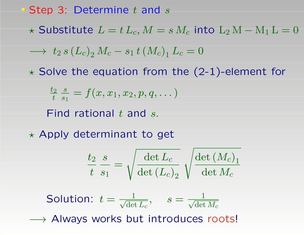
• Step 3: Determine t and s

? Substitute L = t Lc,M = sMc into L2 M−M1 L = 0

−→ t2 s (Lc)2Mc − s1 t (Mc)1 Lc = 0

? Solve the equation from the (2-1)-element for

t2t

ss1

= f(x, x1, x2, p, q, . . . )

Find rational t and s.

? Apply determinant to get

t2

t

s

s1=

√detLc

det (Lc)2

√det (Mc)1

detMc

Solution: t = 1√detLc

, s = 1√detMc

−→ Always works but introduces roots!

The ratiot2

t

s

s1is invariant under the change

t→a1

at, s→

a2

as,

where a(x) is arbitrary.

Proper choice of a(x) =⇒ Rational t and s.

No roots needed!

Lax Pair Algorithm – Systems of P∆Es

(Nijhoff 2001, Bobenko and Suris 2001)

Applies to systems of P∆Es that are

consistent around the cube

Example 2: Schwarzian-Boussinesq System

z1 y − x1 + x = 0

z2 y − x2 + x = 0

z y12(y1 − y2)− y(p y2 z1 − q y1 z2) = 0

• Note: System has two single-edge equations and

one full-face equation

• Edge equations require augmentation of system

with additional shifted, edge equations

z12 y2 − x12 + x2 = 0

z12 y1 − x12 + x1 = 0

• Edge equations will provide additional constraints

during homogenization (Step 2).

• Step 1: Verify the consistency around the cube

? System on the front face:

z1y − x1 + x = 0

z2y − x2 + x = 0

z12y2 − x12 + x2 = 0

z12y1 − x12 + x1 = 0

zy12(y1 − y2)− y(py2z1 − qy1z2) = 0

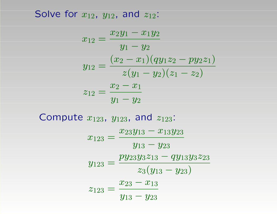
Solve for x12, y12, and z12:

x12 =x2y1 − x1y2

y1 − y2

y12 =(x2 − x1)(qy1z2 − py2z1)

z(y1 − y2)(z1 − z2)

z12 =x2 − x1

y1 − y2

Compute x123, y123, and z123:

x123 =x23y13 − x13y23

y13 − y23

y123 =py23y3z13 − qy13y3z23

z3(y13 − y23)

z123 =x23 − x13

y13 − y23

? System on the bottom face:

z1y − x1 + x = 0

z3y − x3 + x = 0

zy13(y1 − y3)− y(py3z1 − ky1z3) = 0

z13y3 − x13 + x3 = 0

z13y1 − x13 + x1 = 0

Solve for x13, y13, and z13:

x13 =x3y1 − x1y3

y1 − y3

y13 =(x2 − x1)(ky1z3 − py3z1)

z(y1 − y3)(z1 − z2)

z13 =x3 − x1

y1 − y3

Compute x123, y123, and z123:

x123 =x23y12 − x12y23

y12 − y23

y123 =py2y23z12 − ky12y2z23

z2(y12 − y23)

z123 =x23 − x12

y12 − y23

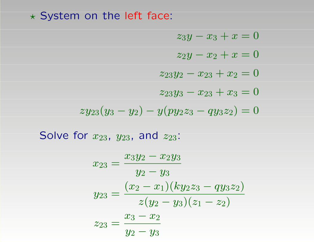
? System on the left face:

z3y − x3 + x = 0

z2y − x2 + x = 0

z23y2 − x23 + x2 = 0

z23y3 − x23 + x3 = 0

zy23(y3 − y2)− y(py2z3 − qy3z2) = 0

Solve for x23, y23, and z23:

x23 =x3y2 − x2y3

y2 − y3

y23 =(x2 − x1)(ky2z3 − qy3z2)

z(y2 − y3)(z1 − z2)

z23 =x3 − x2

y2 − y3

Compute x123, y123, and z123:

x123 =x13y12 − x12y13

y12 − y13

y123 =qy1y13z12 − ky1y12z13

z1(y12 − y13)

z123 =x13 − x12

y12 − y13

Substitute x12, y12, y12, x13, y13, z13, x23, y23, z23

into the above to get

x123 =(pz1(x3y2− x2y3)+ qz2(x1y3− x3y1)+ kz3(x2y1− x1y2)

(pz1(y2 − y3) + qz2(y3 − y1) + kz3(y1 − y2)

y123=pqy3z1(x2−x1)+kpy2z1(x1−x3)+kqy1(x3z2−x1z2+x1z3−x2z3)

z1(pz1(y2 − y3) + qz2(y3 − y1) + kz3(y1 − y2))

z123 =z(z1− z2)(x3(y1− y2) + x1(y2− y3)+ x2(y3− y1))

(x1 − x2)(pz1(y2 − y3) + qz2(y3 − y1) + kz3(y1 − y2))

Answer is unique and independent of x and y.

Consistency around the cube is satisfied!

• Step 2: Homogenization

? Observed that x3, y3 and z3 appear linearly in

numerators and denominators of

x13 =y1(x+ yz3)− y3(x+ yz1)

y1 − y3

y13 =pyy3z1 − kyy1z3

z(y1 − y3)

z13 =y(z3 − z1)

y1 − y3

x23 =y2(x+ yz3)− y3(x+ yz2)

y2 − y3

y23 =qyy3z2 − kyy2z3

z(y2 − y3)

z23 =y(z3 − z2)

y2 − y3

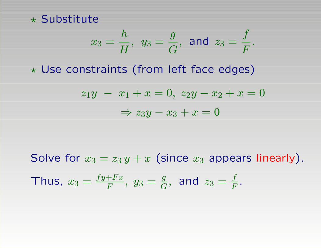
? Substitute

x3 =h

H, y3 =

g

G, and z3 =

f

F.

? Use constraints (from left face edges)

z1y − x1 + x = 0, z2y − x2 + x = 0

⇒ z3y − x3 + x = 0

Solve for x3 = z3 y + x (since x3 appears linearly).

Thus, x3 = fy+FxF

, y3 = gG, and z3 = f

F.

? Substitute x3, y3, z3 into x13, y13, z13:

x13 =Fgx− FGxy1 − fGyy1 + Fgyz1

F (g −Gy1)

y13 =y(fGky1 − Fgpz1)

F (g −Gy1)z

z13 =Gy(Fz1 − f)

F (g −Gy1)

Require that numerators and denominators are

linear in f, F, g, and G. That forces G = F .

Hence, x3 = fy+FxF

, y3 = gF, and z3 = f

F.

? Compute

x3 =fy + Fx

F−→ x13 =

f1y1 + F1x1

F1

y3 =g

F−→ y13 =

g1

F1

z3 =f

F−→ z13 =

f1

F1

Hence,

x13 =−fyy1 + g(x+ yz1)− Fxy1

g − Fy1=f1y1 + F1x1

F1

y13 =y(fky1 − gpz1)

(g − Fy1)z=g1

F1

z13 =y(−f + Fz1)

g − Fy1=f1

F1

Note that

x13 =−fyy1 + g(x+ yz1)− Fxy1

g − Fy1=f1y1 + F1x1

F1

is automaticlly satisfied as a result of the relationx3 = z3 y + x.

? Write in matrix form:

ψ1 =

f1

g1

F1

= t

−y 0 yz1

kyy1z−pyz1

z0

0 1 −y1

f

g

F

= Lψ

? Repeat the same steps for x23, y23, z23 to obtain

ψ2 =

f2

g2

F2

= t

−y 0 yz2

kyy2z− qyz2

z0

0 1 −y2

f

g

F

= M ψ

? Therefore,

L = tLc = t

−y 0 yz1

kyy1z−pyz1

z0

0 1 −y1

M = sMc = s

−y 0 yz2

kyy2z− qyz2

z0

0 1 −y2

• Step 3: Determine t and s

? Substitute L = t Lc,M = sMc into L2 M−M1 L = 0

−→ t2 s (Lc)2Mc − s1 t (Mc)1 Lc = 0

? Solve the equation from the (2-1)-element:

t2t

ss1

= y1y2.

Thus, t = s = 1y, or t = 1

y1and s = 1

y2,

or t = 3

√z

y2y1z1and s = 3

√z

y2y2z2.

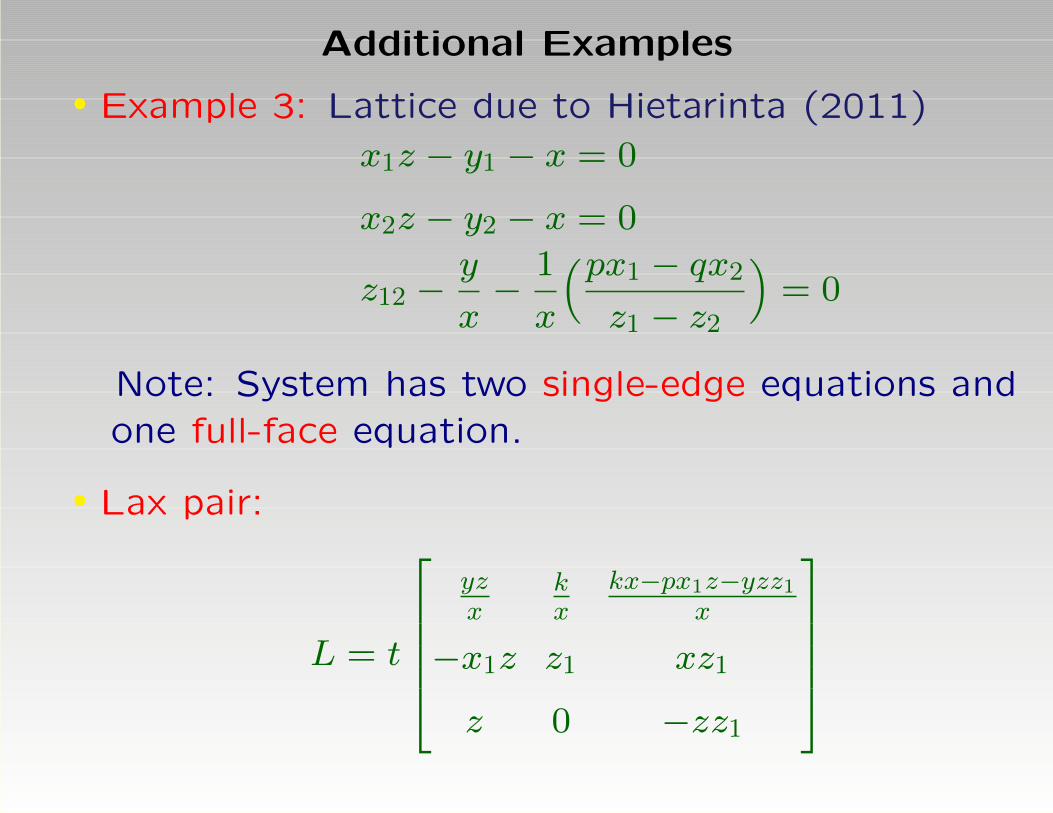
Additional Examples

• Example 3: Lattice due to Hietarinta (2011)x1z − y1 − x = 0

x2z − y2 − x = 0

z12 −y

x−

1

x

(px1 − qx2

z1 − z2

)= 0

Note: System has two single-edge equations andone full-face equation.

• Lax pair:

L = t

yzx

kx

kx−px1z−yzz1x

−x1z z1 xz1

z 0 −zz1

and

M = s

yzx

kx

kx−qx2z−yzz2x

−x2z z2 xz2

z 0 −zz2

,where t = s = 1

z, or t = 1

z1, s = 1

z2,

or t = 3

√x

x1z2z1, s = 3

√x

x2z2z2.

Here, t2t

ss1

= z1z2.

• Example 4: Discrete Boussinesq System

(Tongas and Nijhoff 2005)

z1 − xx1 + y = 0

z2 − xx2 + y = 0

(x2 − x1)(z − xx12 + y12)− p+ q = 0

• Lax pair:

L = t

−x1 1 0

−y1 0 1

p− k − xy1 + x1z −z x

M = s

−x2 1 0

−y2 0 1

q − k − xy2 + x2z −z x

with t = s = 1, or t = 1

3√p−k and s = 13√q−k .

Note: x3 = fF, y3 = g

F, and ψ =

f

F

g

, and t2t

ss1

= 1.

• Example 5: System of pKdV Lattices

(Xenitidis and Mikhailov 2009)

(x− x12)(y1 − y2)− p2 + q2 = 0

(y − y12)(x1 − x2)− p2 + q2 = 0

• Lax pair:

L =

0 0 tx t(p2 − k2 − xy1)

0 0 t −ty1

Ty T (p2 − k2 − x1y) 0 0

T −Tx1 0 0

M =

0 0 sx s(q2 − k2 − xy2)

0 0 s −sy2

Sy S(q2 − k2 − x2y) 0 0

S −Sx2 0 0

with t = s = T = S = 1,

or t T = 1√DetLc

= 1p−k and s S = 1√

DetMc= 1

q−k .

Note: t2T

Ss1

= 1 and T2t

sS1

= 1,

or T2TSS1 = 1, with T = t T, S = s S.

Here, x3 = fF, y3 = g

G, and ψ = [f F g G]T .

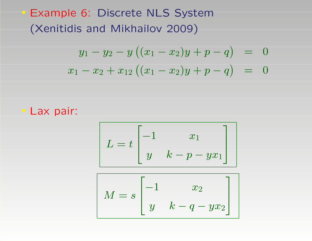
• Example 6: Discrete NLS System

(Xenitidis and Mikhailov 2009)

y1 − y2 − y((x1 − x2)y + p− q

)= 0

x1 − x2 + x12

((x1 − x2)y + p− q

)= 0

• Lax pair:

L = t

−1 x1

y k − p− yx1

M = s

−1 x2

y k − q − yx2

with t = s = 1, or t= 1√DetLc

= 1√α−k and s= 1√

β−k .

Note: x3 = fF

, ψ =

fF

, and t2t

ss1

= 1.

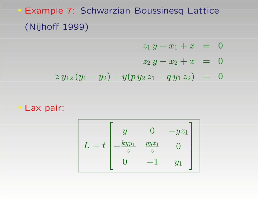
• Example 7: Schwarzian Boussinesq Lattice

(Nijhoff 1999)

z1 y − x1 + x = 0

z2 y − x2 + x = 0

z y12 (y1 − y2)− y(p y2 z1 − q y1 z2) = 0

• Lax pair:

L = t

y 0 −yz1

−kyy1z

pyz1z

0

0 −1 y1

M = s

y 0 −yz2

−kyy2z

pyz2z

0

0 −1 y2

with t = s = 1

y, or t = 1

y1and s = 1

y2,

or t = 3

√z

y2y1z1and s = 3

√z

y2y2z2.

Note: x3 = fy+FxF

, y3 = gF, z3 = f

F, ψ =

f

g

F

,

and t2t

ss1

= y1y2.

• Example 9: Toda modified Boussinesq System

(Nijhoff 1992)

y12(p− q + x2 − x1)− (p− 1)y2 + (q − 1)y1 = 0

y1y2(p− q − z2 + z1)− (p− 1)yy2 + (q − 1)yy1 = 0

y(p+ q − z − x12)(p− q + x2 − x1)− (p2 + p+ 1)y1

+ (q2 + q + 1)y2 = 0• Lax pair:

L= t

k + p− z 1+k+k2

y−k2y−y1−p2(y1−y)−ky(x1−z)+yzx1

y

−p(y1+yx1+yz)y

0 p− 1 (1− k)y1

1 0 p− k − x1

M=s

k + q − z 1+k+k2

y−k2y−y2−q2(y2−y)−ky(x2−z)+yzx2

y

− q(y2+yx2+yz)y

0 q − 1 (1− k)y2

1 0 q − k − x2

with t = s = 1, or t = 3

√y1y

and s = 3

√y2y

.

Note: x3 = fF, y3 = g

F, ψ =

f

g

F

Here, t2

tss1

= 1.

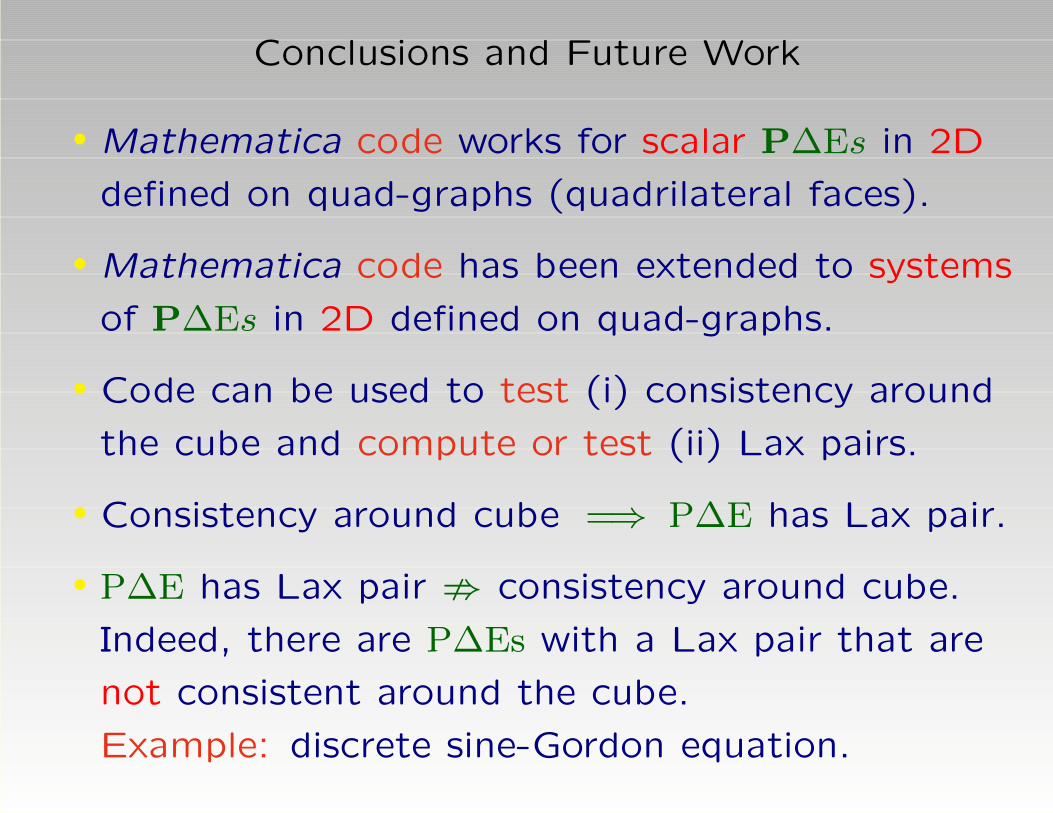
Conclusions and Future Work

• Mathematica code works for scalar P∆Es in 2D

defined on quad-graphs (quadrilateral faces).

• Mathematica code has been extended to systems

of P∆Es in 2D defined on quad-graphs.

• Code can be used to test (i) consistency around

the cube and compute or test (ii) Lax pairs.

• Consistency around cube =⇒ P∆E has Lax pair.

• P∆E has Lax pair ; consistency around cube.

Indeed, there are P∆Es with a Lax pair that are

not consistent around the cube.

Example: discrete sine-Gordon equation.

• Avoid the determinant method to avoid square

roots! Factorization plays an essential role!

• Hard cases: Q4 equation (elliptic curves,

Weierstraß functions) (Nijhoff 2001) and Q5

• Future Work: Extension to more complicated

systems of P∆Es.

• P∆Es in 3D: Lax pair will be expressed in terms of

tensors. Consistency around a “hypercube”.

Examples: discrete Kadomtsev-Petviashvili (KP)

equations.

Thank You

Additional Examples

• Example 9: (H1) Equation (ABS classification)

(x− x12)(x1 − x2) + q − p = 0

• Lax pair:

L = t

x p− k − xx1

1 −x1

M = s

x q − k − xx2

1 −x2

with t = s = 1 or t = 1√

k−p and s = 1√k−q

Note: t2t

ss1

= 1.

• Example 10: (H2) Equation (ABS 2003)

(x−x12)(x1−x2)+(q−p)(x+x1+x2+x12)+q2−p2 =0

• Lax pair:

L = t

p− k + x p2 − k2 + (p− k)(x+ x1)− xx1

1 −(p− k + x1)

M = s

q − k + x q2 − k2 + (q − k)(x+ x2)− xx2

1 −(q − k + x2)

with t = 1√

2(k−p)(p+x+x1)and s = 1√

2(k−q)(q+x+x2)

Note: t2t

ss1

= p+x+x1q+x+x2

.

• Example 11: (H3) Equation (ABS 2003)

p(xx1 + x2x12)− q(xx2 + x1x12) + δ(p2 − q2) = 0

• Lax pair:

L = t

kx −(δ(p2 − k2) + pxx1

)p −kx1

M = s

kx −(δ(q2 − k2) + qxx2

)q −kx2

with t = 1√

(p2−k2)(δp+xx1)and s = 1√

(q2−k2)(δq+xx2)

Note: t2t

ss1

= δp+xx1δq+xx2

.

• Example 12: (H3) Equation (δ = 0) (ABS 2003)

p(xx1 + x2x12)− q(xx2 + x1x12) = 0

• Lax pair:

L = t

kx −pxx1

p −kx1

M = s

kx −qxx2

q −kx2

with t = s = 1

xor t = 1

x1and s = 1

x2

Note: t2t

ss1

= xx1xx2

= x1x2.

• Example 13: (Q1) Equation (ABS 2003)

p(x−x2)(x1−x12)−q(x−x1)(x2−x12)+δ2pq(p−q) = 0

• Lax pair:

L = t

(p− k)x1 + kx −p(δ2k(p− k) + xx1

)p −

((p− k)x+ kx1

)

M = s

(q − k)x2 + kx −q(δ2k(q − k) + xx2

)q −

((q − k)x+ kx2

)

with t = 1δp±(x−x1)

and s = 1δq±(x−x2)

,

or t = 1√k(p−k)((δp+x−x1)(δp−x+x1))

and

s = 1√k(q−k)((δq+x−x2)(δq−x+x2))

Note: t2t

ss1

=q(δp+(x−x1))(δp−(x−x1))p(δq+(x−x2))(δq−(x−x2))

.

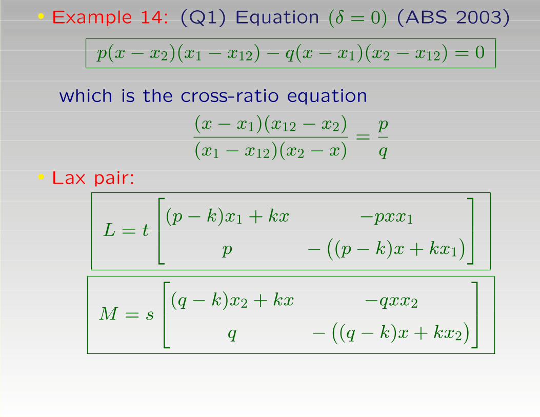
• Example 14: (Q1) Equation (δ = 0) (ABS 2003)

p(x− x2)(x1 − x12)− q(x− x1)(x2 − x12) = 0

which is the cross-ratio equation

(x− x1)(x12 − x2)

(x1 − x12)(x2 − x)=p

q

• Lax pair:

L = t

(p− k)x1 + kx −pxx1

p −((p− k)x+ kx1

)

M = s

(q − k)x2 + kx −qxx2

q −((q − k)x+ kx2

)

Here, t2t

ss1

= q(x−x1)2

p(x−x2)2. So, t = 1

x−x1 and s = 1x−x2

or t = 1√k(k−p)(x−x1)

and s = 1√k(k−q)(x−x2)

.

• Example 15: (Q2) Equation (ABS 2003)

p(x−x2)(x1−x12)−q(x−x1)(x2−x12)+pq(p−q)

(x+x1+x2+x12)−pq(p−q)(p2−pq+q2)=0

• Lax pair:

L= t

(k−p)(kp−x1)+kx

−p(k(k−p)(k2−kp+p2−x−x1)+xx1

)p −

((k−p)(kp−x)+kx1

)

M=s

(k−q)(kq−x2)+kx

−q(k(k−q)(k2−kq+q2−x−x2)+xx2

)q −

((k−q)(kq−x)+kx2

)

• with

t = 1√k(k−p)((x−x1)2−2p2(x+x1)+p4)

and

s = 1√k(k−q)((x−x2)2−2q2(x+x2)+q4)

Note:

t2

t

s

s1=

q((x− x1)2 − 2p2(x+ x1) + p4

)p((x− x2)2 − 2q2(x+ x2) + q4

)=

p((X +X1)2 − p2

) ((X −X1)2 − p2

)q((X +X2)2 − q2

) ((X −X2)2 − q2

)with x = X2, and, consequently, x1 = X2

1 , x2 = X22 .

• Example 16: (Q3) Equation (ABS 2003)

(q2−p2)(xx12+x1x2)+q(p2−1)(xx1+x2x12)

−p(q2−1)(xx2+x1x12)−δ2

4pq(p2−q2)(p2−1)(q2−1)=0

• Lax pair:

L= t

−4kp

(p(k2−1)x+(p2−k2)x1

)−(p2−1)(δ2k2−δ2k4−δ2p2+δ2k2p2−4k2pxx1)

−4k2p(p2−1) 4kp(p(k2−1)x1+(p2−k2)x

)

M=s

−4kq

(q(k2−1)x+(q2−k2)x2

)−(q2−1)(δ2k2−δ2k4−δ2q2+δ2k2q2−4k2qxx2)

−4k2q(q2−1) 4kq(q(k2−1)x2+(q2−k2)x

)

• with

t= 1

2k√p(k2−1)(k2−p2)(4p2(x2+x21)−4p(1+p2)xx1+δ2(1−p2)2)

and

s= 1

2k√q(k2−1)(k2−q2)(4q2(x2+x22)−4q(1+q2)xx2+δ2(1−q2)2)

.

Note:

t2

t

s

s1

=q(q2−1)

(4p2(x2+x2

1)−4p(1+p2)xx1+δ2(1−p2)2)

p(p2−1)(4q2(x2+x2

2)−4q(1+q2)xx2+δ2(1−q2)2)

=q(q2−1)

(4p2(x−x1)2−4p(p−1)2xx1+δ2(1−p2)2

)p(p2−1)

(4q2(x−x2)2−4q(q−1)2xx2+δ2(1−q2)2

)=q(q2−1)

(4p2(x+x1)2−4p(p+1)2xx1+δ2(1−p2)2

)p(p2−1)

(4q2(x+x2)2−4q(q+1)2xx2+δ2(1−q2)2

)

where

4p2(x2+x21)−4p(1+p2)xx1+δ2(1−p2)2

= δ2(p−eX+X1)(p−e−(X+X1))(p−eX−X1)(p−e−(X−X1))

= δ2(p−cosh(X +X1)+sinh(X +X1))

(p−cosh(X +X1)−sinh(X +X1))

(p−cosh(X −X1)+sinh(X −X1))

(p−cosh(X −X1)−sinh(X −X1))

with x = δ cosh(X), and, consequently,

x1 = δ cosh(X1), x2 = δ cosh(X2).

• Example 17: (Q3) Equation (δ) = 0 (ABS 2003)

(q2 − p2)(xx12 + x1x2) + q(p2 − 1)(xx1 + x2x12)

−p(q2 − 1)(xx2 + x1x12) = 0

• Lax pair:

L= t

(p2−k2)x1+p(k2−1)x −k(p2−1)xx1

(p2−1)k −((p2−k2)x+p(k2−1)x1

)

M=s

(q2−k2)x2+q(k2−1)x −k(q2−1)xx2

(q2−1)k −((q2−k2)x+q(k2−1)x2

)

• with t = 1px−x1 and s = 1

qx−x2

or t = 1px1−x and s = 1

qx2−x

or t = 1√(k2−1)(p2−k2)(px−x1)(px1−x)

and s = 1√(k2−1)(q2−k2)(qx−x2)(qx2−x)

.

Note: t2t

ss1

= (q2−1)(px−x1)(px1−x)(p2−1)(qx−x2)(qx2−x)

.

• Example 18: (α, β)-equation (Quispel 1983)((p−α)x−(p+β)x1

) ((p−β)x2−(p+α)x12

)−((q−α)x−(q+β)x2

) ((q−β)x1−(q+α)x12

)=0

• Lax pair:

L= t

(p−α)(p−β)x+(k2−p2)x1 −(k−α)(k−β)xx1

(k+α)(k+β) −((p+α)(p+β)x1+(k2−p2)x

)

M=s

(q−α)(q−β)x+(k2−q2)x2 −(k−α)(k−β)xx2

(k+α)(k+β) −((q+α)(q+β)x2+(k2−q2)x

)

• with t = 1(α−p)x+(β+p)x1)

and s = 1(α−q)x+(β+q)x2)

or t = 1(β−p)x+(α+p)x1)

and s = 1(β−q)x+(α+q)x2)

or t = 1√(p2−k2)((β−p)x+(α+p)x1)((α−p)x+(β+p)x1)

and s = 1√(q2−k2)((β−q)x+(α+q)x2)((α−q)x+(β+q)x2)

Note: t2t

ss1

=((β−p)x+(α+p)x1)((α−p)x+(β+p)x1)((β−q)x+(α+q)x2)((α−q)x+(β+q)x2)

.

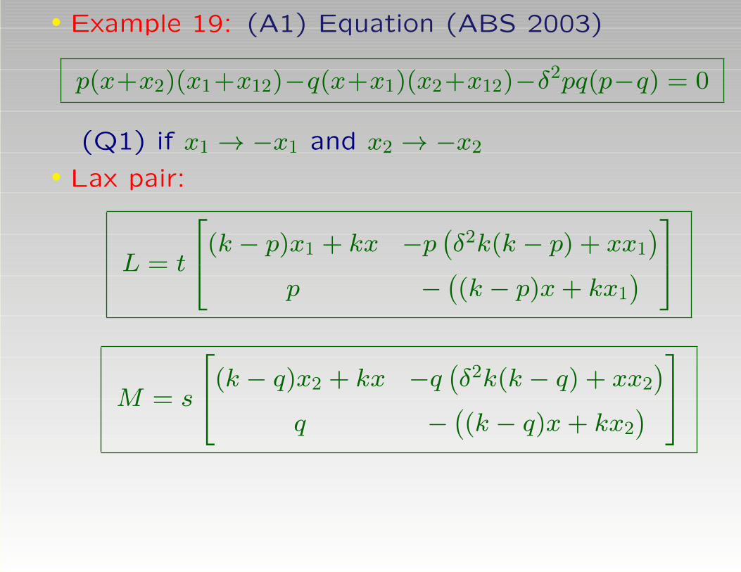
• Example 19: (A1) Equation (ABS 2003)

p(x+x2)(x1+x12)−q(x+x1)(x2+x12)−δ2pq(p−q) = 0

(Q1) if x1 → −x1 and x2 → −x2

• Lax pair:

L = t

(k − p)x1 + kx −p(δ2k(k − p) + xx1

)p −

((k − p)x+ kx1

)

M = s

(k − q)x2 + kx −q(δ2k(k − q) + xx2

)q −

((k − q)x+ kx2

)

• with t = 1√k(k−p)((δp+x+x1)(δp−x−x1))

and

s = 1√k(k−q)((δq+x+x2)(δq−x−x2))

Note: t2t

ss1

=q(δp+(x+x1))(δp−(x+x1))p(δq+(x+x2))(δq−(x+x2))

.

Question: Rational choice for t and s?

• Example 20: (A2) Equation (ABS 2003)

(q2 − p2)(xx1x2x12 + 1) + q(p2 − 1)(xx2 + x1x12)

−p(q2 − 1)(xx1 + x2x12) = 0

(Q3) with δ = 0 via Mobius transformation:

x→ x, x1 → 1x1, x2 → 1

x2, x12 → x12, p→ p, q → q

• Lax pair:

L= t

k(p2−1)x −(p2−k2+p(k2−1)xx1

)p(k2−1)+(p2 − k2)xx1 −k(p2−1)x1

M=s

k(q2−1)x −(q2−k2+q(k2−1)xx2

)q(k2−1)+(q2−k2)xx2 −k(q2−1)x2

• with t = 1√(k2−1)(k2−p2)(p−xx1)(pxx1−1)

and s = 1√(k2−1)(k2−q2)(q−xx2)(qxx2−1)

Note: t2t

ss1

= (q2−1)(p−xx1)(pxx1−1)(p2−1)(q−xx2)(qxx2−1)

.

Question: Rational choice for t and s?

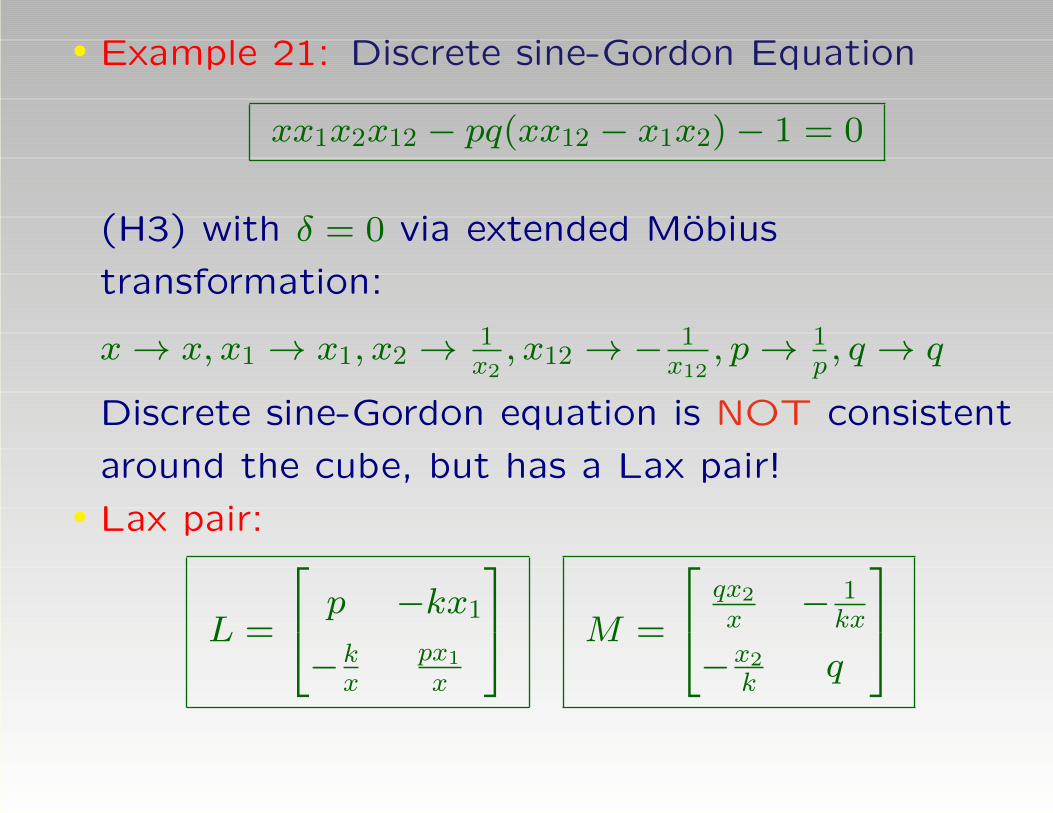
• Example 21: Discrete sine-Gordon Equation

xx1x2x12 − pq(xx12 − x1x2)− 1 = 0

(H3) with δ = 0 via extended Mobius

transformation:

x→ x, x1 → x1, x2 → 1x2, x12 → − 1

x12, p→ 1

p, q → q

Discrete sine-Gordon equation is NOT consistent

around the cube, but has a Lax pair!• Lax pair:

L =

p −kx1

−kx

px1x

M =

qx2x− 1kx

−x2k

q