Embed Size (px)
Citation preview
Symbolic Abstraction: Algorithms and Applications
by
Aditya V. Thakur
A dissertation submitted in partial fulfillment of
the requirements for the degree of
Doctor of Philosophy
(Computer Sciences)
at the
UNIVERSITY OF WISCONSIN–MADISON
2014
Date of final oral examination: 08/08/2014
The dissertation is approved by the following members of the Final Oral Committee:
Thomas W. Reps, Professor, Computer SciencesSomesh Jha, Professor, Computer SciencesKenneth L. McMillan, Senior Researcher, Microsoft ResearchC. David Page Jr., Professor, Biostatistics & Medical Informatics, and Computer SciencesMooly Sagiv, Professor, School of Computer Science, Tel Aviv UniversityXiaojin Zhu, Associate Professor, Computer Sciences

© Copyright by Aditya V. Thakur 2014
All Rights Reserved

i

ii
Acknowledgments
I would like to thank Prof. Thomas Reps. Without his guidance and encouragement this thesis
would not have materialized. As an adviser, he taught me about computer science, about research,
about teaching, about writing, about the ’which’ that should have been a ’that’, about the power
of the haka dance, and about pronouncing names of French computer scientists. As a student, I
hope I was not a complete disappointment.
Prof. Mooly Sagiv hosted me during two wonderful and useful visits to Tel Aviv. The first
trip was a few months after I had embarked on generalizing Stålmarck’s method; the discussions
in Tel Aviv helped solidify a lot of ideas presented in this thesis. During the second trip, Mooly’s
three wonderful daughters taught me how to swing upside-down on a monkey bar (and I also
worked on the research that led to Chapter 12).
Prof. Somesh Jha was always willing to impart useful advice, provided I reviewed a paper
for him in return—I think I owe him at least four reviews.
The rest my thesis committee, Dr. Kenneth McMillan, Prof. David Page, and Prof. Xiaojin
Zhu, asked a lot of interesting questions during my defense and gave many useful comments,
which greatly improved the presentation of the dissertation.
I would have given up on pursuing a Ph.D. if it were not for the encouragement and confidence
of Prof. R. Govindarajan, my adviser during my Master’s at IISc, Bangalore.
Evan Driscoll was always a careful reader of my drafts and a constructive critic of my pre-
sentations. He was a sounding board for my ideas, and patient with my many questions on
the vagaries of languages, compilers, and linkers. It was a wonderful experience writing the
OpenNWA tool with Evan.

iii
I has always been a learning experience working with Akash Lal during the time we over-
lapped at UW, and during later collaborations when he moved to Microsoft Research.
I did not get an opportunity to work with Nick Kidd while he was at UW, though I did
interact with him during my work on the OpenNWA tool, which was built on top of the WAli tool
written by Akash and Nick. I got an opportunity to work with Nick this last year, partly because
he was assigned to be my Google Mentor. The distributed SAT solver (Chapter 10) would not
have been built without his help. I learned a lot from him in the short time we collaborated.
It was a wonderful experience working with Jason Breck on SMASLTOV. I wish him the very
best for his graduate career.
Junghee Lim developed the TSL infrastructure, which was used in much of the research on
machine-code verification done in this dissertation.
The folks at GrammaTech, Inc., especially Brian Alliet, Denis Gopan, Alexey Loginov, and
Suan Hsi Yong, provided tool support and help for the work I carried out on machine-code
analysis.
Madison was a more fun place because of the dinners, dances, and drives with Gopika Nair.
The group that organized Diwali Night, especially Prachi, Muffi, Divya, and Rika, brought
out talents in me that I never realized I had.
The Southwest chicken sandwich never tasted the same at The Library (Bar & Cafe) after
Andres Jaan Tack left for Estonia.
Tristan Ravitch and I shared a passion for pl-eating and Mickies Dairy Bar. One day we
shall write a SAT solver in Haskell.
Dean Sanders provided me with multiple drama-free years while sharing an apartment. We
played the longest chess game of my life, and our discussions on astronomy and biology were
always insightful.
Tycho Andersen kept me sane in Madison, and was also an awesome companion on many
travels around the world. With him, I discovered spewn, ridin’ dirty, and DUM DUM DUM.
Cindy Rubio González read many a drafts, commented on presentations, and was always
there for me.

iv
My parents have always provided me with unconditional love and support. As a son, I hope
I am not a complete disappointment. To them, I dedicate this thesis. My parents would often
remark how little they understand about my research. The dedication is written in Marathi so as
to provide at least one page that is incomprehensible to my thesis committee and completely
understandable to my parents.
My dissertation research was supported, in part, by AFOSR under grant FA9550-09-1-0279;
NSF under grants CCF-0540955, CCF-0810053, and CCF-0904371; ONR under grants N00014-10-
M-0251 and N00014-11-C-0447; ARL under grant W911NF-09-1-0413; DARPA under cooperative
agreement HR0011-12-2-0012; and a Google Ph.D. Fellowship. Any opinions, findings, and
conclusions or recommendations expressed in this dissertation are those of the author, and do
not necessarily reflect the views of the sponsoring agencies.

v
Contents
Contents v
List of Tables ix
List of Figures xii
Abstract xvii
1 Through the Lens of Abstraction 1
1.1 Abstraction in Program Verification . . . . . . . . . . . . . . . . . . . . . . . . . . . . 4
1.2 Abstraction in Decision Procedures . . . . . . . . . . . . . . . . . . . . . . . . . . . . 11
1.3 The different hats of α . . . . . . . . . . . . . . . . . . . . . . . . . . . . . . . . . . . . 12
1.4 Thesis Outline . . . . . . . . . . . . . . . . . . . . . . . . . . . . . . . . . . . . . . . 18
1.5 Suggested Order of Reading . . . . . . . . . . . . . . . . . . . . . . . . . . . . . . . . 21
1.6 Chapter Notes . . . . . . . . . . . . . . . . . . . . . . . . . . . . . . . . . . . . . . . . 23
2 There’s Plenty of Room at the Bottom 24
2.1 The Need for Machine-Code Analysis . . . . . . . . . . . . . . . . . . . . . . . . . . . 25
2.2 The Challenges in Machine-Code Analysis . . . . . . . . . . . . . . . . . . . . . . . . . 26
2.3 The Design Space for Machine-Code Analysis . . . . . . . . . . . . . . . . . . . . . . . 29
2.4 Chapter Notes . . . . . . . . . . . . . . . . . . . . . . . . . . . . . . . . . . . . . . . . 32
3 Preliminaries 33

vi
3.1 Abstract Interpretation . . . . . . . . . . . . . . . . . . . . . . . . . . . . . . . . . . . 33
3.2 Symbolic Abstract Interpretation . . . . . . . . . . . . . . . . . . . . . . . . . . . . . . 40
3.3 Decision Procedures . . . . . . . . . . . . . . . . . . . . . . . . . . . . . . . . . . . . . 45
3.4 Stålmarck’s Method for Propositional Logic . . . . . . . . . . . . . . . . . . . . . . . . 46
3.5 Chapter Notes . . . . . . . . . . . . . . . . . . . . . . . . . . . . . . . . . . . . . . . . 51
4 Symbolic Abstraction from Below 53
4.1 RSY Algorithm . . . . . . . . . . . . . . . . . . . . . . . . . . . . . . . . . . . . . . . 54
4.2 KS Algorithm . . . . . . . . . . . . . . . . . . . . . . . . . . . . . . . . . . . . . . . . 57
4.3 Empirical Comparison of the RSY and KS Algorithms . . . . . . . . . . . . . . . . . . . 58
5 A Bilateral Algorithm for Symbolic Abstraction 62
5.1 Towards a Bilateral Algorithm . . . . . . . . . . . . . . . . . . . . . . . . . . . . . . . 63
5.2 A Parametric Bilateral Algorithm . . . . . . . . . . . . . . . . . . . . . . . . . . . . . 64
5.3 Abstract Domains with Infinite Descending Chains . . . . . . . . . . . . . . . . . . . . 72
5.4 Instantiations . . . . . . . . . . . . . . . . . . . . . . . . . . . . . . . . . . . . . . . . 76
5.5 Empirical Comparison of the KS and Bilateral Algorithms . . . . . . . . . . . . . . . . . 82
5.6 Computing Post . . . . . . . . . . . . . . . . . . . . . . . . . . . . . . . . . . . . . . 84
5.7 Related Work . . . . . . . . . . . . . . . . . . . . . . . . . . . . . . . . . . . . . . . . 84
5.8 Chapter Notes . . . . . . . . . . . . . . . . . . . . . . . . . . . . . . . . . . . . . . . . 88
6 A Generalization of Stålmarck’s Method 90
6.1 Overview . . . . . . . . . . . . . . . . . . . . . . . . . . . . . . . . . . . . . . . . . . 93
6.2 Algorithm for A ˜ssume[ϕ](A) . . . . . . . . . . . . . . . . . . . . . . . . . . . . . . . . 99
6.3 Instantiations . . . . . . . . . . . . . . . . . . . . . . . . . . . . . . . . . . . . . . . . 108
6.4 Experimental Evaluation . . . . . . . . . . . . . . . . . . . . . . . . . . . . . . . . . . 110
6.5 Related Work . . . . . . . . . . . . . . . . . . . . . . . . . . . . . . . . . . . . . . . . 114
6.6 Chapter Notes . . . . . . . . . . . . . . . . . . . . . . . . . . . . . . . . . . . . . . . . 114
7 Computing Best Inductive Invariants 116

vii
7.1 Basic Insights . . . . . . . . . . . . . . . . . . . . . . . . . . . . . . . . . . . . . . . . 118
7.2 Best Inductive Invariants and Intraprocedural Anaysis . . . . . . . . . . . . . . . . . . 119
7.3 Best Inductive Invariants and Interprocedural Analysis . . . . . . . . . . . . . . . . . . 125
7.4 Related Work . . . . . . . . . . . . . . . . . . . . . . . . . . . . . . . . . . . . . . . . 127
7.5 Chapter Notes . . . . . . . . . . . . . . . . . . . . . . . . . . . . . . . . . . . . . . . . 128
8 Bit-Vector Inequality Domain 129
8.1 The BVI Abstract Domain . . . . . . . . . . . . . . . . . . . . . . . . . . . . . . . . . 133
8.2 Related Work . . . . . . . . . . . . . . . . . . . . . . . . . . . . . . . . . . . . . . . . 138
8.3 Chapter Notes . . . . . . . . . . . . . . . . . . . . . . . . . . . . . . . . . . . . . . . . 139
9 Symbolic Abstraction for Machine-Code Verification 140
9.1 Background on Directed Proof Generation (DPG) . . . . . . . . . . . . . . . . . . . . . 142
9.2 MCVETO . . . . . . . . . . . . . . . . . . . . . . . . . . . . . . . . . . . . . . . . . . 143
9.3 Implementation . . . . . . . . . . . . . . . . . . . . . . . . . . . . . . . . . . . . . . . 158
9.4 Experimental Evaluation . . . . . . . . . . . . . . . . . . . . . . . . . . . . . . . . . . 159
9.5 Related Work . . . . . . . . . . . . . . . . . . . . . . . . . . . . . . . . . . . . . . . . 161
9.6 Chapter Notes . . . . . . . . . . . . . . . . . . . . . . . . . . . . . . . . . . . . . . . . 163
10 A Distributed SAT Solver 164
10.1 The DiSSolve Algorithm . . . . . . . . . . . . . . . . . . . . . . . . . . . . . . . . . . 166
10.2 Experimental Evaluation . . . . . . . . . . . . . . . . . . . . . . . . . . . . . . . . . . 171
10.3 Generalization . . . . . . . . . . . . . . . . . . . . . . . . . . . . . . . . . . . . . . . . 177
10.4 Related Work . . . . . . . . . . . . . . . . . . . . . . . . . . . . . . . . . . . . . . . . 180
10.5 Chapter Notes . . . . . . . . . . . . . . . . . . . . . . . . . . . . . . . . . . . . . . . . 181
11 Satisfiability Modulo Abstraction for Separation Logic with Linked Lists 182
11.1 Separation Logic and Canonical Abstraction . . . . . . . . . . . . . . . . . . . . . . . . 185
11.2 Overview . . . . . . . . . . . . . . . . . . . . . . . . . . . . . . . . . . . . . . . . . . 191
11.3 Proof System for Separation Logic . . . . . . . . . . . . . . . . . . . . . . . . . . . . . 197

viii
11.4 Experimental Evaluation . . . . . . . . . . . . . . . . . . . . . . . . . . . . . . . . . . 201
11.5 Related Work . . . . . . . . . . . . . . . . . . . . . . . . . . . . . . . . . . . . . . . . 205
11.6 Future Work . . . . . . . . . . . . . . . . . . . . . . . . . . . . . . . . . . . . . . . . . 207
11.7 Chapter Notes . . . . . . . . . . . . . . . . . . . . . . . . . . . . . . . . . . . . . . . . 208
12 Property-Directed Symbolic Abstraction 209
12.1 The Property-Directed Inductive Invariant (PDII) Algorithm . . . . . . . . . . . . . . . 212
12.2 Chapter Notes . . . . . . . . . . . . . . . . . . . . . . . . . . . . . . . . . . . . . . . . 217
13 Conclusion 219
13.1 Abstract Interpretation . . . . . . . . . . . . . . . . . . . . . . . . . . . . . . . . . . . 220
13.2 Machine-Code Verification . . . . . . . . . . . . . . . . . . . . . . . . . . . . . . . . . 224
13.3 Decision Procedures . . . . . . . . . . . . . . . . . . . . . . . . . . . . . . . . . . . . . 225
References 229

ix
List of Tables
1.1 Chapters relevant to a particular topic . . . . . . . . . . . . . . . . . . . . . . . . . . . 22
3.1 Examples of conjunctive domains. v, vi represent program variables and c, ci represent
constants . . . . . . . . . . . . . . . . . . . . . . . . . . . . . . . . . . . . . . . . . . . . 36
4.1 The characteristics of the x86 binaries of Windows utilities used in the experiments.
The columns show the number of instructions (instrs); the number of procedures
(procs); the number of basic blocks (BBs); the number of branch instructions (brs). . 59
5.1 Qualitative comparison of symbolic-abstraction algorithms. A 3 indicates that the
algorithm has a property described by a column, and a 7 indicates that the algorithm
does not have the property. . . . . . . . . . . . . . . . . . . . . . . . . . . . . . . . . . 63
5.2 Performance and precision comparison between the KS and Bilateral algorithms. The
columns show the times, in seconds, for α↑KS and αl〈E232〉WPDS construction; the
number of invocations of α↑KS that had a decision procedure timeout (t/o); and the
degree of improvement gained by using αl〈E232〉-generated weights rather than α↑KS
weights (measured as the percentage of control points whose inferred one-vocabulary
affine relation was strictly more precise under αl〈E232〉-based analysis). . . . . . . . 83
6.1 The characteristics of the x86 binaries of Windows utilities used in the experiments.
The columns show the number of instructions (instrs); the number of procedures
(procs); the number of basic blocks (BBs); the number of branch instructions (brs). . 110

x
6.2 Time taken, in seconds, by the αl and α↓ algorithms for WPDS construction. The
subscript is used to denote the time limit used for a single invocation of a call to α:
t = ∞ denotes that no time limit was given, and t = 1 denotes that a time limit of
1 second was given. For each benchmark, the algorithm that takes the least time is
highlighted in bold. . . . . . . . . . . . . . . . . . . . . . . . . . . . . . . . . . . . . . 111
6.3 Comparison of the degree of improvement gained by using αlt=∞ and α↓t=1 (measured
as the percentage of control points for which the inferred one-vocabulary affine
relation inferred by one analysis was strictly more precise than that inferred by the
other analysis). . . . . . . . . . . . . . . . . . . . . . . . . . . . . . . . . . . . . . . . . 112
9.1 Machine-code verification experiments. The first column displays the test name. The
Expected column lists the expected answer: [ ] means the target PC is reachable,
[9] means the target PC is unreachable. The ’BVI’ column displays the time taken
(in seconds) and the answer obtained when performing analysis based on the BVI
abstract domain; [ ? ] means the analysis could not determine whether or not the
target PC was reachable. No total timeout was specified for the BVI analysis. The
’MCVETO’ column displays the time taken (in seconds) by MCVETO when not using
any speculative trace refinement. The MCVETO+ column displays the time taken (in
seconds) by MCVETO when using speculative trace refinement. [—] means MCVETO
or MCVETO+ timed out after 100 seconds. . . . . . . . . . . . . . . . . . . . . . . . . . 160
10.1 Run time, in seconds, for DiSSolve on an 8-core machine. The number of compute
engines (or cores) available to DiSSolve was 8; the value of k was chosen to be 4. (The
names of some of the benchmarks have been truncated due to space constraints.) . . 176
10.2 Run time, in seconds, for DiSSolve when run on the cloud. c denotes the number of
compute engines available to DiSSolve, and k is the number of splitting variables. . 176
11.1 Core predicates used when representing states made up of acyclic linked lists. . . . 187

xi
11.2 Voc consists of the predicates shown above, together with the ones in Table 11.1. All
unary predicates are abstraction predicates; that is, A = Voc1. . . . . . . . . . . . . . 197
11.3 Number of formulas that contain each of the SL operators in Groups 1, 2, and 3. The
columns labeled “+” and “−” indicate the number of atoms occurring as positive
and negative literals, respectively. . . . . . . . . . . . . . . . . . . . . . . . . . . . . . 201
11.4 Unsatisfiable formulas. The time is in seconds. . . . . . . . . . . . . . . . . . . . . . . 203
11.5 Example instantiations of T1def= ¬a ∧ emp ∧ (a ∗ b), where a, b ∈ Literals. The time is
in seconds. . . . . . . . . . . . . . . . . . . . . . . . . . . . . . . . . . . . . . . . . . . 204
11.6 Example instantiations of T2def= emp∧a∧(b∗(c−~(emp∧¬a))), where a, b, c ∈ Literals.
The time is in seconds. . . . . . . . . . . . . . . . . . . . . . . . . . . . . . . . . . . . . 205
xii
List of Figures
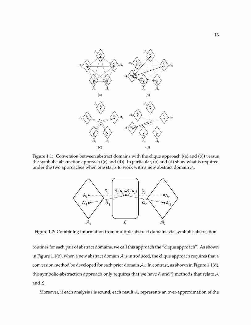
1.1 Conversion between abstract domains with the clique approach ((a) and (b)) versus
the symbolic-abstraction approach ((c) and (d)). In particular, (b) and (d) show what
is required under the two approaches when one starts to work with a new abstract
domain A. . . . . . . . . . . . . . . . . . . . . . . . . . . . . . . . . . . . . . . . . . . . 13
1.2 Combining information from multiple abstract domains via symbolic abstraction. . 13
1.3 An example of how information from the Parity and Interval domains can be used to
improve each other via symbolic abstraction. . . . . . . . . . . . . . . . . . . . . . . . 14
1.4 Dependencies among chapters . . . . . . . . . . . . . . . . . . . . . . . . . . . . . . . 22
2.1 A program that, on some executions, can modify the return address of foo so that
foo returns to the beginning of bar, thereby reaching ERR. (MakeChoice is a primitive
that returns a random 32-bit number.) . . . . . . . . . . . . . . . . . . . . . . . . . . . 30
2.2 Conventional ICFG for the program shown in Figure 2.1. Note that the CFG for bar
is disconnected from the rest of the ICFG. . . . . . . . . . . . . . . . . . . . . . . . . . 31
3.1 Integrity constraints corresponding to the formula ϕ = (a ∧ b) ∨ (¬a ∨ ¬b). The root
variable of ϕ is u1. . . . . . . . . . . . . . . . . . . . . . . . . . . . . . . . . . . . . . . 47
3.2 Propagation rules. . . . . . . . . . . . . . . . . . . . . . . . . . . . . . . . . . . . . . . . 47
3.3 Proof that ϕ is valid. . . . . . . . . . . . . . . . . . . . . . . . . . . . . . . . . . . . . . 48
3.4 The Dilemma Rule. . . . . . . . . . . . . . . . . . . . . . . . . . . . . . . . . . . . . . . 48
xiii
3.5 Sequence of Dilemma Rules in a proof that ψ is valid. (Details of 0-saturation steps
are omitted. For brevity, singleton equivalence-classes are not shown.) . . . . . . . . 49
3.6 Stålmarck’s method. The operation Close performs transitive closure on a formula
relation after new tuples are added to the relation. . . . . . . . . . . . . . . . . . . . 50
4.1 Total time taken by all invocations of α↑RSY[E232 ] compared to that taken by α↑KS for each
of the benchmark executables. The running time is normalized to the corresponding
time taken by α↑RSY[E232 ]; lower numbers are better. . . . . . . . . . . . . . . . . . . . 59
4.2 (a) Scatter plot showing of the number of decision-procedure queries during each pair
of invocations of α↑RSY and α↑KS, when neither invocation had a decision-procedure
timeout. (b) Log-log scatter plot showing the times taken by each pair of invocations
of α↑RSY and α↑KS, when neither invocation had a decision-procedure timeout. . . . . 60
5.1 Abstract Consequence: For all a1, a2 ∈Awhere γ(a1)( γ(a2), if a = AbstractConsequence(a1, a2),
then γ(a1) ⊆ γ(a) and γ(a) 6⊇ γ(a2). . . . . . . . . . . . . . . . . . . . . . . . . . . . . 65
5.2 The two cases arising in Algorithm 11: ϕ ∧ ¬γ(p) is either (a) unsatisfiable, or (b)
satisfiable with S |= ϕ and S 6|= γ(p). (Note that although lower v α(ϕ) v upper and
JϕK ⊆ γ(upper) are invariants of Algorithm 11, γ(lower) ⊆ JϕK does not necessarily
hold, as depicted above.) . . . . . . . . . . . . . . . . . . . . . . . . . . . . . . . . . . 66
5.3 Iterations of Algorithm 11 in Example 5.5. Self-mappings, e.g., y 7→ y, are omitted. . 79
5.4 Iterations of Algorithm 11 in Example 5.6. Self-mappings, e.g., y 7→ y, are omitted. . 80
5.5 Abstract consequence on polyhedra. (a) Two polyhedra: lower v upper. (b) p =
AbstractConsequence(lower,upper). (c) Result of upper← upper u p. . . . . . . . . . 82
6.1 Examples of propagation rules for inequality relations on literals. . . . . . . . . . . . 94
6.2 0-saturation proof that χ is valid, using inequality relations on literals. . . . . . . . . 94
6.3 (a) Inconsistent inequalities in the (unsatisfiable) formula used in Example 6.3. (b)
Application of the Dilemma Rule to abstract value (P0, A0). The dashed arrows from
(Pi, Ai) to (P ′i , A′i) indicate that (P ′i , A′i) is a semantic reduction of (Pi, Ai). . . . . . . 96

xiv
6.4 Rules used to convert a formula ϕ ∈ L into a set of integrity constraints I. op
represents any binary connective in L, and literal(L) is the set of atomic formulas
and their negations. . . . . . . . . . . . . . . . . . . . . . . . . . . . . . . . . . . . . . 101
6.5 Boolean rules used by Algorithm 17 in the call InternalRule(J, (P,A)). . . . . . . . . 106
6.6 Rules used by Algorithm 17 in the call LeafRule(J, (P,A)). . . . . . . . . . . . . . . . 106
6.7 Semilog plot of Z3 vs. α↓ on χd formulas. . . . . . . . . . . . . . . . . . . . . . . . . . 113
7.1 (a) Example program. (b) Dependences among node-variables in the program’s
equation system (over node-variables {V1, V6, V12}). (c) The transition relations among
{V1, V6, V12} (expressed as formulas). . . . . . . . . . . . . . . . . . . . . . . . . . . . 120
7.2 A possible chaotic-iteration sequence when a BII solver is invoked to find the best
inductive affine-equality invariant for Equation (7.2). The parts of the trace enclosed in
boxes show the actions that take place in calls to Algorithm 8 (Post↑). (By convention,
primes are dropped from the abstract value returned from a call on Post↑.) . . . . . 122
7.3 A possible trace of Iteration 2 from Figure 7.2 when the call to Post↑
(Algorithm 8) is
replaced by a call to Postl
(Algorithm 15). . . . . . . . . . . . . . . . . . . . . . . . . 123
7.4 The effect of specializing the abstract pre-condition at enter node ep, and the resulting
strengthening of the inferred abstract post-condition. (The abstract domain is the
domain of affine equalities E232 .) . . . . . . . . . . . . . . . . . . . . . . . . . . . . . . 127
8.1 Each + represents a solution of the indicated inequality in 4-bit unsigned bit-vector
arithmetic. . . . . . . . . . . . . . . . . . . . . . . . . . . . . . . . . . . . . . . . . . . . 131
9.1 The general refinement step across frontier (n, I,m). The presence of a witness is
indicated by a “�” inside of a node. . . . . . . . . . . . . . . . . . . . . . . . . . . . . 142
9.2 (a) A program with a non-deterministic branch; (b) the program’s ICFG. . . . . . . . 144
9.3 (a) Internal-transitions in the initial NWA-based abstract graphG0 created by MCVETO;
(b) call- and return-transitions in G0. * is a wild-card symbol that matches all instruc-
tions. . . . . . . . . . . . . . . . . . . . . . . . . . . . . . . . . . . . . . . . . . . . . . . 146

xv
9.4 (a) and (b) show two generalized traces, each of which reaches the end of the program.
(c) shows the intersection of the two generalized traces. (“�” indicates that a node
has a witness.) . . . . . . . . . . . . . . . . . . . . . . . . . . . . . . . . . . . . . . . . . 147
9.5 Definition of the trace-folding operation π/[PC]. . . . . . . . . . . . . . . . . . . . . . 148
9.6 Figures 9.4(a) and 9.4(b) with the loop-head in adjust split with respect to the candi-
date invariant ϕ def= x+ y = 500. . . . . . . . . . . . . . . . . . . . . . . . . . . . . . . 152
9.7 Programs that illustrate the benefit of using a conceptually infinite abstract graph. . 152
9.8 ERR is reachable, but only along a path in which a ret instruction serves to perform a
call. . . . . . . . . . . . . . . . . . . . . . . . . . . . . . . . . . . . . . . . . . . . . . . . 156
10.1 Log-log scatter plot comparing the running time (in seconds) of ppfolio[c = 8] and
DiSSolve[c = 23, k = 4] on 150 unsatisfiable (UNSAT) benchmarks. . . . . . . . . . . 173
10.2 Cactus plot comparing the running time (in seconds) of ppfolio[c = 8] and DiSSolve[c =
23, k = 4] on 150 unsatisfiable (UNSAT) benchmarks. . . . . . . . . . . . . . . . . . . 174
10.3 Log-log scatter plot comparing the running time (in seconds) of ppfolio[c = 8] and
DiSSolve[c = 23, k = 4] on 150 satisfiable (SAT) benchmarks. . . . . . . . . . . . . . 175
10.4 Cactus plot comparing the running time (in seconds) of ppfolio[c = 8] and DiSSolve[c =
23, k = 4] on 150 unsatisfiabile (UNSAT) benchmarks. . . . . . . . . . . . . . . . . . . 177
10.5 Each call to Deduce in AbstractDissolveSplit works on a different, though not nec-
essarily disjoint, portion of the search space. The dot-shaded sub-lattice (on the
left) is searched for models of ϕ that satisfy the (abstract) assumption A1. The solid-
filled sub-lattice (on the right) is searched for models of ϕ that satisfy the (abstract)
assumption A2. . . . . . . . . . . . . . . . . . . . . . . . . . . . . . . . . . . . . . . . . 179
10.6 Each call to Deduce in AbstractDissolveSplit infers (possibly different) globally true
abstract values A′1 and A′2, where ϕ⇒ γ(A′1) and ϕ⇒ γ(A′2). These two branches are
then merged by performing a meet. . . . . . . . . . . . . . . . . . . . . . . . . . . . . . 180
11.1 Satisfaction of an SL formula ϕ with respect to statelet (s, h). . . . . . . . . . . . . . . 186
11.2 Structures that arise in the meet operation used to analyze x 7→ y ∗ y 7→ x. . . . . . . 192

xvi
11.3 Some of the structures that arise in the meet operation used to evaluate x 7→ y −~
ls(x, z). . . . . . . . . . . . . . . . . . . . . . . . . . . . . . . . . . . . . . . . . . . . . . 195
11.4 Rules for computing an abstract value that overapproximates the meaning of a formula
in SL . . . . . . . . . . . . . . . . . . . . . . . . . . . . . . . . . . . . . . . . . . . . . . . 197
11.5 The abstract value for ls(x, y) ∈ atom in the canonical-abstraction domain. . . . . . . 198
11.6 The abstract value for [di = dj · dk]] in the canonical-abstraction domain. . . . . . . . 198
xvii
Abstract
This dissertation explores the use of abstraction in two areas of automated reasoning: verifica-
tion of programs, and decision procedures for logics. Establishing that a program is correct
is undecidable in general. Program-verification tools sidestep this tar-pit of undecidability by
working on an abstraction of a program, which over-approximates the original program’s behav-
ior. The theory underlying this approach is called abstract interpretation. Developing a scalable
and precise abstract interpreter is a challenging problem, especially when analyzing machine
code. Abstraction provides a new language for the description of decision procedures, leading to
new insights. I call such an abstraction-centric view of decision procedures Satisfiability Modulo
Abstraction (SMA).
The unifying theme behind the dissertation is the concept of symbolic abstraction:
Given a formula ϕ in logic L and an abstract domain A, the symbolic abstraction of
ϕ is the strongest consequence of ϕ expressible in A.
This dissertation advances the field of abstract interpretation by presenting two new algorithms
for performing symbolic abstraction, which can be used to synthesize various operations required
by an abstract interpreter. The dissertation presents two new algorithms for computing inductive
invariants for programs. The dissertation shows how the use of symbolic abstraction enables the
design of a new abstract domain capable of representing bit-vector inequality invariants.
The dissertation advances the field of machine-code analysis by showing how symbolic
abstraction can be used to implement machine-code analyses. Furthermore, the dissertation
describes MCVETO, a new model-checking algorithm for machine code.

xviii
The dissertation advances the field of decision procedures by presenting a variety of SMA
solvers. One is based on a generalization of Stålmarck’s method, a decision procedure for
propositional logic. When viewed through the lens of abstraction, Stålmarck’s method can be
lifted from propositional logic to richer logics, such as linear rational arithmetic. Furthermore,
the SMA view shows that the generalized Stålmarck’s method actually performs symbolic
abstraction. Thus, the concept of symbolic abstraction brings forth the connection between
abstract interpretation and decision procedures. The dissertation describes a new distributed
decision procedure for propositional logic, called DiSSolve. Finally, the dissertation presents an
SMA solver for a new fragment of separation logic.
1
Chapter 1
Through the Lens of Abstraction
Cubism came about because, in the process of analyzing form, something
that lay in the form, a plane, could be lifted out to float on its own.— Joseph Plaskett
This thesis explores the use of abstraction in two areas of automated reasoning: verification of
programs, and decision procedures for logics.
Establishing that a program is correct is undecidable in general. Program-verification tools
sidestep this tar-pit of undecidability by working on an abstraction of a program, which over-
approximates the original program’s behavior. The theory underlying this approach is called
abstract interpretation (Cousot and Cousot, 1977), and is around forty years old. However, devel-
oping a scalable and precise abstract interpreter still remains a challenging problem.
This thesis also explores the use of abstraction in the design and implementation of decision
procedures. Abstraction provides a new language for the description of decision procedures,

2
leading to new insights and new ways of thinking. I call such an abstraction-centric view of
decision procedures Satisfiability Modulo Abstraction.
The common use of abstraction in this work also brings out a non-trivial and useful relation-
ship between program verification and decision procedures.
The Need for Program Verification
Quis custodiet ipsos custodes?
Who will guard the guards themselves?— Satires of Juvenal
Software is everywhere. There is an increasing use of computers in our daily lives. More
importantly, safety-critical and security-critical computer systems are becoming ubiquitous.
Computers are an integral part of communication systems, flight systems, financial systems,
power systems, and medical systems. Furthermore, the functionality and complexity of these
computer systems has also increased. With this pervasive use of computers it is becoming
increasingly important to develop formal methods that certify that a given program is correct.
There is an economic argument—faulty software costs the U.S. economy at least $5 billion per
year (Charette, 2005)—as well as a moral argument—errors in safety-critical systems could lead
to loss of life (Bowen, 2000; Abramson and Pike, 2011)—for formal verification of computer
programs.
Ideally, one would like to establish that a computer programP strictly adheres to its functional,
safety, and security specification—that is, P satisfies a given property I for all possible inputs. In
theory, determining whether P satisfies I is undecidable. In practice, the program-verification
problem is often addressed by focusing on a restricted set of properties; however, the complexity
and size of the software makes program verification difficult even when the class of properties
to be verified is restricted. It is the goal of formal methods to make the practice of program
verification feasible for industrial-scale systems. Instead of verifying full functional correctness,
most program-verification tools verify comparatively “shallow”, yet critical, safety properties of

3
programs, such as absence of null-pointer dereferences, absence of out-of-bounds array accesses,
absence of division by zero, and verification of data-structure invariants.
In the last two decades, there has been tremendous innovation in formal verification, and a
greater adoption of formal methods, resulting in various industrial-scale tools being developed
(Holzmann, 2004; Ball et al., 2004; Delmas and Souyris, 2007; Jetley et al., 2008; Bessey et al.,
2010; Chapman and Schanda, 2014). However, implementing a correct, precise, and scalable
program-verification tool is an onerous and formidable task. Furthermore, as the analyses
and techniques become more complex, the need for automating the construction of such tools
increases (Cuoq et al., 2012).
The Emergence of a Disruptive Technology
(It is shown that) any recognition problem solved by a polynomial time-bounded
nondeterministic Turing machine can be “reduced” to the problem of determining
whether a given propositional formula is a tautology.— Stephen A. Cook (1971)
A decision procedure for a logic L is an algorithm that given a formula ϕ ∈ L determines
whether (i) ϕ is satisfiable if there exists an assignment to the variables of ϕ that satisfies ϕ, or (ii) ϕ
is unsatisfiable if no such satisfying assignment exists. A decision procedure for propositional logic
is called a SAT solver. For example, given the propositional-logic formula ψ1 := p1∧p2∧ (p3∨p4),
a SAT solver would determine thatψ1 is satisfiable with the following (Boolean) assignment to the
variables: [p1 7→ true, p2 7→ true, p3 7→ false, p4 7→ true]. Although propositional satisfiability
is an NP-complete problem, the last fifteen years have born witness to a wide range of SAT
solvers that are efficient for deciding satisfiability of formulas with millions of variables arising
in practical applications. Furthermore, decision procedures for richer logics, called Satisfiability
Modulo Theories (SMT) solvers, have been implemented. This tremendous progress in SAT and
SMT solvers has resulted in new, practical solutions to a wide variety of problems, including
planning problems (Kautz and Selman, 1992; Rintanen, 2009), cryptanalysis (Massacci and
Marraro, 2000), bounded model checking (Biere, 2009), program synthesis (Alur et al., 2013),

4
and automated test-input generation (Godefroid et al., 2005). The application of SMT solvers to
automated test-input generation leads us to the topic of the next section.
From Paths in Program to Formulas in Logic
Testing shows the presence, not the absence of bugs.
— Edsger W. Dijkstra (1969)
Suppose that we are asked to determine whether the ERROR statement is reachable in thefollowing C-code snippet:
i f ( x < y ) {i f (2∗ x+3∗z < w) {
}e lse {
ERROR:}
}
It should be clear that the ERROR statement is reachable if and only if the following formula in
quantifier-free bit-vector logic (QFBV) is satisfiable: (x < y) ∧ ¬(2x+ 3z < w). Thus, we already
see a (rather weak) connection between program verification and decision procedures—namely,
the conversion of a particular path in a program to a formula in a logic.
Unfortunately, most programs have loops, procedure calls, and recursion. Consequently,
the number of paths that could reach a particular statement is large (or even infinite). Hence, it
is not possible to check feasibility of each such path using a decision procedure. This simple
observation motivates the use of abstraction in program verification.
1.1 Abstraction in Program Verification
Abstract interpretation (Cousot and Cousot, 1977) provides a way to obtain information about
the possible states that a program reaches during execution, but without actually running the
program on specific inputs. Instead, it explores the program’s behavior for all possible inputs,
thereby accounting for all possible states that the program can reach.

5
Before describing the basic concepts of abstract interpretation, I first describe concrete in-
terpretation of programs. A concrete state of a program characterizes the state of the program
at a particular point during program execution, and typically consists of the valuations of the
various program variables. For instance, if x and y are integer program variables, a concrete
state σ would be described as [x 7→ 3, y 7→ 42]. (The similarity between the notation used for
describing concrete states of programs and models of formulas is not coincidental.) The concrete
interpretation of a program gives a concrete transformer that describes, for each program statement,
how a single (input) concrete state is transformed into a single (output) concrete state according
to the semantics of the programming language1. For instance, given the statement S ≡ x := x + 5,
which increments the value of variable x by 5, the concrete state σ would be transformed into
the output concrete state σ′ = [x′ 7→ 8, y′ 7→ 42]; the primes on the variables are merely used to
denote that these variables are in the output state.
In contrast to the situation in concrete interpretation, the abstract states during abstract inter-
pretation are finite-sized descriptors that represent a collection of concrete states. For instance, an
abstract state a =[x 7→ [2, 10], y 7→ [20, 200]
]denotes the set of concrete states in which variable
x takes values from the interval from 2 to 10 (inclusive), and variable y takes values from the
interval from 20 to 200 (inclusive). The collection of abstract states or abstract values form a lattice
called an abstract domain. The collection of concrete states described by an abstract value a is
denoted by γ(a). For example, the abstract value a is a value in the abstract domain of intervals
Interval. Various such abstract domains can be defined, each differing in what aspects of the
collection of concrete states they capture. For example, one can use abstract states that represent
only the sign of a variable’s value: neg, zero, pos, or unknown.
Paralleling the scenario in the concrete world, in abstract interpretation an abstract transformer
describes how, for each program statement, an input abstract state gets transformed into an
output abstract state. The abstract transformer should be sound with respect to the corresponding
concrete transformer; that is, the abstract transformer should be an over-approximation of the
concrete transformer. For example, given the input abstract state a and the statement S, the1For simplicity of exposition, the discussion here is restricted to deterministic semantics.

6
output abstract state is a′ =[x′ 7→ [7, 15], y′ 7→ [20, 200]
]. Because each abstract state represents a
collection of concrete states, operationally, one can think of abstract interpretation as running
the program “in the aggregate.” This seemingly simple concept of abstract interpretation has led
to much beautiful theory that helps reason about the soundness of sophisticated static analyses
of programs. In particular, as long as the abstract transformer is an over-approximation of the
concrete semantics of the program, the program properties inferred by the abstract interpreter
describe a superset of the states that can actually occur, and can be used as invariants.
Abstract Domains as Logic Fragments
An abstract domain A can be seen as a logic fragment, and each abstract value can be expressed
as a formula in this logic fragment. Let LA be some fragment of a general-purpose logic L. We
say that γ is a symbolic-concretization operation if it maps each A ∈ A to ϕA ∈ LA such that the
meaning of ϕA equals the collection of concrete states described by A; that is, JϕAK = γ(A). LA
is often defined by a syntactic restriction on the formulas of L.
Example 1.1. For instance, for abstract states over intervals, LInterval is the set of conjunctions
of one-variable inequalities over the program variables. Our experience is that it is generally
easy to implement the γ operation for an abstract domain. For example, given A ∈ Interval, it is
straightforward to read off the appropriate ϕA ∈ LInterval: each entry x 7→ [clow, chigh] contributes
the conjuncts “clow ≤ x” and “x ≤ chigh.” �
Symbolic Abstraction
Unfortunately, the theory of abstract interpretation does not provide algorithms for computing
the abstract transformers from the concrete transformers. Consequently, in practice, an analysis
writer needs to manually write the abstract transformers for each concrete operation. This task
can be tedious and error-prone, especially for machine code where most instructions involve
bit-wise operations. Thus, abstract interpretation has a well-deserved reputation of being a kind
of “black art”, and consequently difficult to work with.

7
Many of the key operations needed by an abstract interpreter, including computing abstract
transformers, can be reduced to the problem of symbolic abstraction (Reps et al., 2004), which
connects abstract interpretation and logic.
Given a formulaϕ in logicL and an abstract domainA, find the strongest consequence
of ϕ expressible in A.
We use αA(ϕ) to denote the symbolic abstraction of ϕ ∈ L with respect to an abstract domain A;
we drop the subscript A from αA(·) when the abstract domain is clear from the context.
Let us see how an algorithm for symbolic abstraction can be used to compute abstract
transformers.
Example 1.2. Consider again the statement S ≡ x := x + 5 and the input abstract value a =[x 7→
[2, 10], y 7→ [20, 200]]
in the abstract domain Interval. The semantics of a concrete operation can
be stated as a formula in a logic L that specifies the relation between input and output states.
In this example, the semantics of the statement S can be expressed in quantifier-free bit-vector
logic (QFBV) as the formula ϕS ≡ x′ = x+ 5. The abstract value a ∈ Interval can be expressed as
a formula γ(a) ≡ (2 ≤ x ≤ 10 ∧ 20 ≤ y ≤ 200).
The output abstract state a′ can be computed as finding the strongest consequence of the
formula ψ ≡ (ϕs ∧ γ(a)) = (2 ≤ x ≤ 10 ∧ 20 ≤ y ≤ 200 ∧ x′ = x+ 5) that can be expressed as an
interval over the variables x′ and y′; that is, α(ψ) =[x′ 7→ [7, 15], y′ 7→ [20, 200]
]. �
Example 1.3 illustrates that applying the abstract transformer can be complex even for a
single machine-code instruction.
Example 1.3. Consider the Intel x86 instruction τ ≡ add bh,al, which adds al, the low-order
byte of 32-bit register eax, to bh, the second-to-lowest byte of 32-bit register ebx. No other register
apart from ebx is modified. For simplicity, we only consider the registers eax, ebx, and ecx. The
semantics of τ can be expressed in QFBV logic as the formula ϕτ :
ϕτdef= ebx′ =
(ebx & 0xFFFF00FF)
| ((ebx + 256 ∗ (eax & 0xFF)) & 0xFF00)
∧ eax′ = eax
∧ ecx′ = ecx,(1.1)

8
where “&” and “|” denote bitwise-and and bitwise-or, respectively, and a symbol with a prime
denotes the value of the symbol in the post-state. Equation (1.1) shows that the semantics of a
seemingly simple add instruction involves non-linear bit-masking operations.
Now suppose that the abstract domain E232 is the domain of affine equalities over the 32-bit
registers eax, ebx, and ecx, and that we would like to compute the abstract transformer for τ when
the input abstract value a ∈ E232 is ebx = ecx. This task corresponds to finding the strongest
consequence of the formula ψ ≡ (ebx = ecx∧ϕτ ) that can be expressed as affine relation among
eax′, ebx′, and ecx′, which turns out to be α(ψ) ≡ (216ebx′ = 216ecx′ + 224eax′) ∧ (224ebx′ =
224ecx′). Multiplying by a power of 2 serves to shift bits to the left; because it is performed in
arithmetic mod 232, bits shifted off the left end are unconstrained. Thus, the first conjunct of
α(ψ) captures the relationship between the low-order two bytes of ebx′, the low-order two bytes
of ecx′, and the low-order byte of eax′. �
My Contributions
In this thesis, I have developed various algorithms for symbolic abstraction, which can be used
to synthesize operations needed by an abstract interpreter. Thus, the use of symbolic abstrac-
tion lessens the burden on analysis designers by raising the level of automation in abstraction
interpretation. Moreover, the use of symbolic abstraction provides help along the following four
dimensions:
soundness: Symbolic abstraction provides a way to create analyzers that are correct-by-construction,
while requiring an analysis designer to implement only a small number of operations.
Consequently, each instantiation of the approach only relies on a small “trusted computing
base”.
precision: Unlike most conventional approaches to creating analyzers, the use of symbolic
abstraction achieves the fundamental limits of precision that abstract-interpretation theory
establishes.

9
scalability: Algorithms for performing symbolic abstraction can be implemented as “anytime”
algorithms—i.e., the algorithms can be equipped with a monitor, and if too much time
or space is being used, the algorithms can be stopped at any time, and a safe (over-
approximating) answer returned. By this means, when the analyzer is applied to a suite
of programs that require successively more analysis resources to be used, precision can
degrade gracefully.
extensibility: If an additional abstract domain is added to an analyzer to track additional in-
formation, information can be exchanged automatically between domains via symbolic
abstraction to produce the most-precise abstract values in each domain. This feature is
illustrated in greater detail in Section 1.3.1.
Symbolic Abstraction and Quantifier Elimination
I now contrast two approaches to computing abstract transformers: (i) the use of symbolic
abstraction, and (ii) the use of quantifier-elimination techniques (Gulwani and Musuvathi, 2008;
Monniaux, 2009, 2010).
Gulwani and Musuvathi (2008) defined what they termed the “cover problem”, which
addresses approximate existential quantifier elimination:
Given a formulaϕ in logicL, and a set of variables V , find the strongest quantifier-free
formula ϕ in L such that J∃V : ϕK ⊆ JϕK.
I use CoverV (ϕ) to denote the cover of ϕ and the set of variables V .
Gulwani and Musuvathi (2008) presented cover algorithms for the theories of uninterpreted
functions and linear arithmetic, and showed that covers exist in some theories that do not support
quantifier elimination.
The notion of a cover has similarities to the notion of symbolic abstraction, but the latter is
more general. If we think of an abstract domain A as a logic fragment L′, then, in purely logical
terms, symbolic abstraction addresses the following problem of performing an over-approximating
translation to an impoverished fragment:
10
Given a formula ϕ in logic L, find the strongest formula ψ in logic-fragment L′ such
that JϕK ⊆ JψK.
Both cover and symbolic abstraction (deliberately) lose information from a given formula ϕ,
and hence both result in over-approximations of JϕK. In general, however, they yield different
over-approximations of JϕK.
1. The information loss from the cover operation only involves the removal of variable set
V from the vocabulary of ϕ. The resulting formula ϕ is still allowed to be an arbitrarily
complex L formula; ϕ can use all of the (interpreted) operators and (interpreted) relation
symbols of L.
2. The information loss from symbolic abstraction involves finding a formulaψ in the fragment
L′: ψ must be a restricted L formula; it can only use the operators and relation symbols of
L′, and must be written using the syntactic restrictions of L′.
One of the uses of information-loss capability 2 is to bridge the gap between the concrete
semantics and an abstract domain. In particular, it may be necessary to use the full power of
logic L to state the concrete semantics of a transformer τ . However, the corresponding abstract
transformer must be expressed in L′. When L′ is something other than the restriction of L to
a sub-vocabulary, cover is not guaranteed to return an answer in L′, and thus does not yield
a suitable abstract transformer. This difference is illustrated using the scenario described in
Example 1.3.
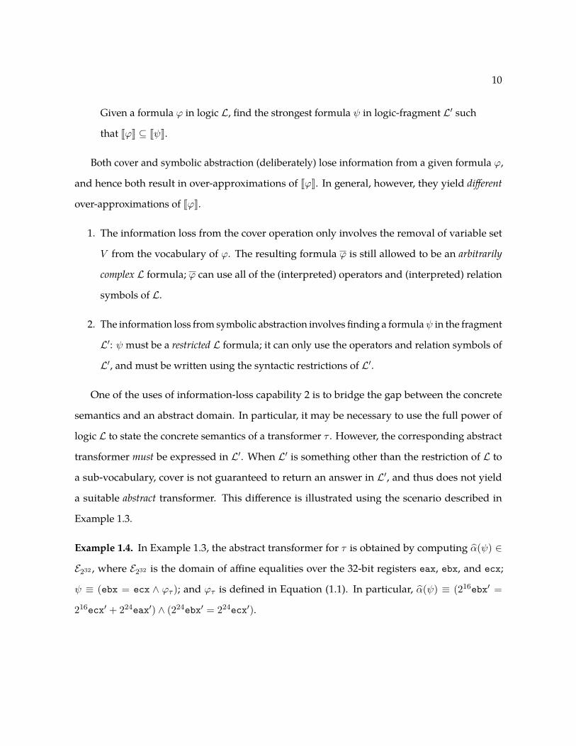
Example 1.4. In Example 1.3, the abstract transformer for τ is obtained by computing α(ψ) ∈
E232 , where E232 is the domain of affine equalities over the 32-bit registers eax, ebx, and ecx;
ψ ≡ (ebx = ecx ∧ ϕτ ); and ϕτ is defined in Equation (1.1). In particular, α(ψ) ≡ (216ebx′ =
216ecx′ + 224eax′) ∧ (224ebx′ = 224ecx′).
11
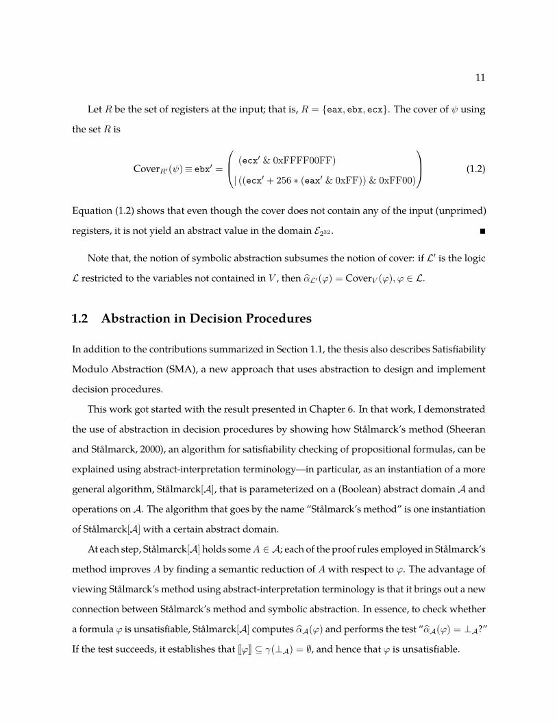
Let R be the set of registers at the input; that is, R = {eax, ebx, ecx}. The cover of ψ using
the set R is
CoverR′(ψ)≡ ebx′ =
(ecx′ & 0xFFFF00FF)
| ((ecx′ + 256 ∗ (eax′ & 0xFF)) & 0xFF00)
(1.2)
Equation (1.2) shows that even though the cover does not contain any of the input (unprimed)
registers, it is not yield an abstract value in the domain E232 . �
Note that, the notion of symbolic abstraction subsumes the notion of cover: if L′ is the logic
L restricted to the variables not contained in V , then αL′(ϕ) = CoverV (ϕ), ϕ ∈ L.
1.2 Abstraction in Decision Procedures
In addition to the contributions summarized in Section 1.1, the thesis also describes Satisfiability
Modulo Abstraction (SMA), a new approach that uses abstraction to design and implement
decision procedures.
This work got started with the result presented in Chapter 6. In that work, I demonstrated
the use of abstraction in decision procedures by showing how Stålmarck’s method (Sheeran
and Stålmarck, 2000), an algorithm for satisfiability checking of propositional formulas, can be
explained using abstract-interpretation terminology—in particular, as an instantiation of a more
general algorithm, Stålmarck[A], that is parameterized on a (Boolean) abstract domain A and
operations onA. The algorithm that goes by the name “Stålmarck’s method” is one instantiation
of Stålmarck[A] with a certain abstract domain.
At each step, Stålmarck[A] holds someA ∈ A; each of the proof rules employed in Stålmarck’s
method improves A by finding a semantic reduction of A with respect to ϕ. The advantage of
viewing Stålmarck’s method using abstract-interpretation terminology is that it brings out a new
connection between Stålmarck’s method and symbolic abstraction. In essence, to check whether
a formula ϕ is unsatisfiable, Stålmarck[A] computes αA(ϕ) and performs the test “αA(ϕ) = ⊥A?”
If the test succeeds, it establishes that JϕK ⊆ γ(⊥A) = ∅, and hence that ϕ is unsatisfiable.

12
Using this abstraction-based view, Stålmarck’s method can be lifted from propositional logic
to richer logics, such as quantifier-free linear rational arithmetic (LRA): to obtain a method for
richer logics, instantiate the parameterized version of Stålmarck’s method with richer abstract
domains, such as the polyhedral domain (Cousot and Halbwachs, 1978). By this means, we
obtained algorithms for computing α for these richer abstract domains. The bottom line is that
our algorithm is “dual-use”:
• it can be used by an abstract interpreter to compute α (and perform other symbolic abstract
operations), and
• it can be used in an SMT solver to determine whether a formula is satisfiable.
One of the main advantages of the SMA approach is that it is able to reuse abstract-interpretation
machinery to implement decision procedures. For instance, in in Chapter 6, the polyhedral
abstract domain—implemented in PPL (Bagnara et al., 2008)—is used to implement an SMA
solver for the logic of linear rational arithmetic. Similarly in Chapter 11, the abstract domain
of shapes—implemented in TVLA (Sagiv et al., 2002)—is used in a novel way to implement an
SMA solver for a new fragment of separation logic for which existing approaches do not apply.
1.3 The different hats of α
In this section, I present some other applications of symbolic abstraction, and draw connections
between symbolic abstraction and concepts used in Machine Learning and Artificial Intelligence.
1.3.1 Communication of Information Between Abstract Domains
Apart from computing abstract transformers, symbolic abstraction also provides a way to combine
the results from multiple analyses automatically—thereby enabling the construction of new,
more-precise analyzers that use multiple abstract domains simultaneously.
Figures 1.1(a) and 1.1(b) show what happens if we want to communicate information between
abstract domains without symbolic abstraction. Because it is necessary to create explicit conversion
13
A1
A1
A2 A
2
A3
A3
A4
A4
A5
A5
(a)
A1
A1
A2 A
2
A3
A3
A4
A4
A5
A5
AA
(b)
A1
A1
A2 A
2
A3
A3
A4
A4
A5
A5
L
(c)
A1
A1
A2 A
2
A3
A3
A4
A4
A5
A5
L
AA
(d)
Figure 1.1: Conversion between abstract domains with the clique approach ((a) and (b)) versusthe symbolic-abstraction approach ((c) and (d)). In particular, (b) and (d) show what is requiredunder the two approaches when one starts to work with a new abstract domain A.
γ1(A1)∧∧∧∧γ2(A2)
A2L
A1
A1
A2
∧∧∧∧ ∧∧∧∧
∧∧∧∧
α1
∧∧∧∧
α2
∧∧∧∧
γ1∧∧∧∧
γ2
A’1 A’2
Figure 1.2: Combining information from multiple abstract domains via symbolic abstraction.
routines for each pair of abstract domains, we call this approach the “clique approach”. As shown
in Figure 1.1(b), when a new abstract domainA is introduced, the clique approach requires that a
conversion method be developed for each prior domainAi. In contrast, as shown in Figure 1.1(d),
the symbolic-abstraction approach only requires that we have α and γ methods that relate A
and L.
Moreover, if each analysis i is sound, each result Ai represents an over-approximation of the

14
L
∧∧∧∧
αP∧∧∧∧
αI
∧∧∧∧
γP∧∧∧∧
γI(axeven,
bxodd,
cxΤ)
(ax[3,12],
bx[5,10],
cx[7,7])
3 ≤ a ≤ 12
∧ 5 ≤ b ≤ 10
∧ 7 ≤ c ≤ 7
∧ 231 a = 0
∧ 231 b = 231
(ax[4,12],
bx[5,9],
cx[7,7])
Parity Interval
(axeven,
bxodd,
cxodd)
Figure 1.3: An example of how information from the Parity and Interval domains can be used toimprove each other via symbolic abstraction.
actual set of concrete states. Consequently, the collection of analysis results {Ai} implicitly tells
us that only the states in⋂i γ(Ai) can actually occur. However, this information is only implicit,
and it can be hard to determine what the intersection value really is.
One way to address this issue is to perform a semantic reduction (Cousot and Cousot, 1979)
of each of the Ai with respect to the set of abstract values {Aj | i 6= j}. Fortunately, symbolic
abstraction provides a way to carry out such semantic reductions without the need to develop
pair-wise or clique-wise reduction operators. The principle is illustrated in Figure 1.2 for the case
of two abstract domains, A1 and A2. Given A1 ∈ A1 and A2 ∈ A2, we can improve the pair
〈A1, A2〉 by first creating the formula ϕ def= γ1(A1) ∧ γ2(A2), and then applying α1 and α2 to ϕ
to obtain A′1 = α1(ϕ) and A′2 = α2(ϕ), respectively. A′1 and A′2 can be smaller than the original
values A1 and A2, respectively. We then use the pair 〈A′1, A′2〉 instead of 〈A1, A2〉. Figure 1.3
shows a specific example of how information from the Parity and Interval domains can be used
to improve each other via the symbolic-abstraction approach to semantic reduction. Note that in
this example
• the Parity value is improved from (a 7→ even, b 7→ odd, c 7→ >) to (a 7→ even, b 7→ odd, c 7→
odd).
• the Interval value is improved from (a 7→ [3, 12], b 7→ [5, 10], c 7→ [7, 7]) to (a 7→ [4, 12], b 7→
[5, 9], c 7→ [7, 7]).

15
When there are more than two abstract domains, we form the conjunction ϕ def=∧i γi(Ai), and
then apply each αi to obtain A′i = αi(ϕ).
1.3.2 Symbolic Abstraction and Interpolation in Logic
Symbolic abstraction also leads to a generalization of interpolation (Craig, 1957), a concept in
mathematical logic. Interpolation has many uses in program verification (Henzinger et al., 2004;
McMillan, 2010).
Definition 1.5. Given ϕ1, ϕ2 ∈ L such that ϕ1⇒ϕ2, I ∈ L is said be an interpolant of ϕ1 and
ϕ2 if and only if (i) ϕ1⇒ I , (ii) I⇒ϕ2, and (iii) I uses only symbols in the shared vocabulary of
ϕ1 and ϕ2. �
A logic L supports interpolation if for all ϕ1, ϕ2 ∈ L, there exists an interpolant I . Many
logics used in verification support interpolation.
In many applications, interpolant I is used as a heuristic for obtaining a simple explanation
of why ϕ1⇒ϕ2. The fact that the interpolant is expressed in terms of the common vocabulary is
what supports the claim that the result is a simple explanation.
Extending our mantra of connecting concepts in logic to those in abstract interpretation, I
introduce the notion of abstract interpolation:
Definition 1.6. Given ϕ1, ϕ2 ∈ L such that ϕ1⇒ϕ2, and an abstract domain A, ι ∈ A is said be
an abstract interpolant of ϕ1 and ϕ2 if and only if (i) ϕ1⇒ γ(ι), and (ii) γ(ι)⇒ϕ2. �
Here there is no common-vocabulary restriction à la Definition 1.5(iii); however, the fact
that ι must be an element of abstract domain A serves as an alternative heuristic for obtaining a
simple explanation.
Note that even if the logic L supports interpolation, it may not necessarily support abstract
interpolation for a given abstract domain A. The existence of an abstract interpolant depends on
the expressiveness of A. When A is defined as the logic L restricted to the symbols common
to ϕ1 and ϕ2, abstract interpolation reduces to standard interpolation. Abstract interpolation

16
generalizes uniform interpolation (Visser, 1996), which is a strengthening of the notion of Craig
interpolation. In uniform interpolation, the interpolant has to be expressed in a given vocabulary
Σ. Thus, uniform interpolation concerns the problem of keeping the vocabulary Σ, and dropping
the rest, which is similar to the cover problem discussed in Section 1.1. Jhala and McMillan
(2006) present an algorithm for computing a uniform interpolant for a limited theory consisting
of restricted use of array operators and rational constraints.
Symbolic abstraction can be used to compute an abstract interpolant. In particular, to compute
an abstract interpolant of ϕ1 and ϕ2, compute ι = α(ϕ1), and verify whether γ(ι)⇒ϕ2. In fact,
this method is guaranteed to compute the strongest abstract interpolant if any abstract interpolant
exists. Thus, the method is sound and complete for abstract domains for which α is computable,
and logics for which validity of implication is decidable. Though I introduce the notion of
abstract interpolation, the rest of the thesis does not further explore this concept.
1.3.3 Symbolic Abstraction in Other Areas of Computer Science
The concept of symbolic abstraction can also be found in the literature on Machine Learning and
Artificial Intelligence.
In (Reps et al., 2004), a connection was made between symbolic abstraction and the problem
of concept learning in (classical) machine learning. In machine-learning terms, an abstract domain
A is a hypothesis space; each domain element corresponds to a concept. A hypothesis space has
an inductive bias, which means that it has a limited ability to express sets of concrete objects.
In abstract-interpretation terms, inductive bias corresponds to the image of γ on A not being
the full power set of the concrete objects—or, equivalently, the image of γ on A being only a
fragment of L. Given a formula ϕ, the symbolic-abstraction problem is to find the most specific
concept that explains the meaning of ϕ.
There are, however, some differences between the problems of symbolic abstraction and
concept learning. These differences mostly stem from the fact that an algorithm for performing
symbolic abstraction already starts with a precise statement of the concept in hand, namely,
the formula ϕ. In the machine-learning context, usually no such finite description of the con-

17
cept exists, which imposes limitations on the types of queries that the learning algorithm can
make to an oracle (or teacher); see, for instance, (Angluin, 1987, Section 1.2). The power of
the oracle also affects the guarantees that a learning algorithm can provide. In particular, in
the machine-learning context, the learned concept is not guaranteed or even required to be
an overapproximation of the underlying concrete concept. During the past three decades, the
machine-learning theory community has shifted their focus to learning algorithms that only
provide probabilistic guarantees. This approach to learning is called probably approximately cor-
rect learning (PAC learning) (Valiant, 1984; Kearns and Vazirani, 1994). The PAC guarantee also
enables a learning algorithm to be applicable to concept lattices that are not complete lattices
(Definition 3.1).
These differences between symbolic abstraction and concept learning serve to highlight the
novelty of the algorithms and applications discussed in the thesis. Furthermore, they also open
up the opportunity for a richer exchange of ideas between the two areas. In particular, one can
imagine situations in which it is appropriate for the overapproximation requirement for abstract
transformers to be relaxed to a PAC guarantee—for example, if abstract interpretation is being
used only to find errors in programs, instead of proving programs correct (Bush et al., 2000), or
if we are analyzing programs with a probabilistic concrete semantics (Kozen, 1981; Monniaux,
2000; Cousot and Monerau, 2012).
The problem of symbolic abstraction is closely related to the problems of restricted consequence
finding (RCF) (McIlraith and Amir, 2001) and approximate knowledge compilation in Artificial
Intelligence (Selman and Kautz, 1996; Del Val, 1999; Simon and Del Val, 2001). Both of these
problems involve translating a formula in a source logic to one in a given (less expressive) target
logic. In the context of knowledge compilation, translating to the target logic allows for efficient
queries to the knowledge base. Most existing techniques for RCF are applicable to propositional
logic or relational first-order logic. Symbolic abstraction also has a connection to another related
problem of forgetting in Artificial Intelligence (Lin and Reiter, 1994, 1997; Eiter and Wang, 2008;
Konev et al., 2009; Wang et al., 2010), which has applications in reuse and combination of
ontologies in Semantic Web applications, cognitive robotics, and logic programming.

18
There has been some work already in connecting some of these problems in Artificial Intelli-
gence to problems in program verification. Jhala and McMillan (2006) apply RCF techniques
to compute interpolants to be used for predicate abstraction. I believe it would be fruitful to
continue exploring this connection between problems in Artificial Intelligence and symbolic
abstraction.
1.4 Thesis Outline
This section provides an outline for each of the chapters in this thesis. Section 1.5 lists the
dependencies the various chapters, and suggests several possible orders in which the chapters
of the thesis can be read. A Chapter Notes section can be found at the end of most chapters.
Those sections provide technical and non-technical background on the research described in the
respective chapter. Chapters 5–12 contain the results developed during my dissertation research,
and present my contributions to advancing the field. Chapter 13 concludes by summarizing the
results in the three research threads discussed in this thesis: abstract interpretation, machine-code
verification, and decision procedures.
Chapter 2: There’s Plenty of Room at the Bottom
In this chapter, I introduce the reader to the unique opportunities and challenges involved in
analyzing machine code. Consequently, this chapter puts into context the tools and techniques
for machine-code analysis and verification developed in this thesis. I also give an overview of
the design space of tools and techniques for machine-code analysis.
Chapter 3: Preliminaries
This chapter introduces and defines concepts in (classical) abstract interpretation and symbolic
abstract interpretation, introduces terminology related to decision procedures, and describes
Stålmarck’s method.

19
Chapter 4: Symbolic Abstraction from Below
In this chapter, I review two prior algorithms for performing symbolic abstraction:
• The RSY algorithm: a framework for computing α that applies to any logic and abstract
domain that satisfies certain conditions (Reps et al., 2004).
• The KS algorithm: an algorithm for computing α that applies to QFBV logic and the domain
E2w of affine equalities (Elder et al., 2011).
I also present the results of an experiment I carried out to compare the performance of the two
algorithms.
Chapter 5: A Bilateral Algorithm for Symbolic Abstraction
This chapter uses the insights gained from the algorithms presented in Chapter 4 to design
a new Bilateral framework for symbolic abstraction that combines the best features of the KS
and RSY algorithms, but also has benefits that none of these previous algorithms have. The
Bilateral framework maintains sound under- and over-approximations of the answer, and hence
the procedure can return the over-approximation if it is stopped at any point (unlike the RSY
and KS algorithms). I compare the performance of the KS algorithm and an instantiation of the
Bilateral framework.
Chapter 6: A Generalization of Stålmarck’s Method
In this chapter, I give a new account of Stålmarck’s method by explaining each of the key
components in terms of concepts from the field of abstract interpretation. In particular, I show
that Stålmarck’s method can be viewed as a general framework, which I call, Stålmarck[A], that
is parameterized by an abstract domain A and operations on A. This abstraction-based view
allows Stålmarck’s method to be lifted from propositional logic to richer logics, such as LRA.
Furthermore, the generalized Stålmarck’s method falls into the Satisfiability Modulo Abstraction

20
(SMA) paradigm: an SMA solver is designed and implemented using concepts from abstract
interpretation.
I also present a connection between symbolic abstraction and Stålmarck’s method for checking
satisfiability, which leads to a new algorithm for symbolic abstraction. I present experimental
results that illustrate the dual-use nature of this Stålmarck-based framework. One experiment
uses it to compute abstract transformers, which are then used to generate invariants; another
experiment uses it for checking satisfiability.
Chapter 7: Computing Best Inductive Invariants
In this chapter, I show how symbolic abstraction can be used to compute best inductive invariants for
an entire program. This chapter provides insight on fundamental limits in abstract interpretation,
because the best inductive invariant represents the limit of obtainable precision for a given abstract
domain.
Chapter 8: Bit-Vector Inequality Domain
In this chapter, I describe how symbolic abstraction enables us to define a new abstract domain,
called the BVI domain, that addresses the following challenges: (1) identifying affine-inequality
invariants while handling overflow in arithmetic operations over bit-vector data-types, and
(2) holding onto invariants about values in memory during machine-code analysis.
Chapter 9: Symbolic Abstraction for Machine-Code Verification
This chapter describes a model-checking algorithm for stripped machine-code called MCVETO
(Machine-Code VErification TOol). I describe how MCVETO adapts directed proof generation (DPG)
(Gulavani et al., 2006) for model checking stripped machine-code. MCVETO implements a new
technique called trace-based generalization, which enables MCVETO to handle instruction aliasing
and self-modifying code. I describe how MCVETO uses speculative trace refinement to use candidate
invariants to speed up the convergence of DPG and to refine the abstraction of the program.
21
Chapter 10: A Distributed SAT Solver
In this chapter, I describe a new distributed SAT algorithm, called DiSSolve, that combines
concepts from Stålmarck’s method with those found in modern SAT solvers. I evaluate the
performance of DiSSolve when deployed on a multi-core machine and on the cloud.
Chapter 11: Satisfiability Modulo Abstraction for Separation Logic with Linked Lists
This chapter describes a procedure for checking the unsatisfiability of formulas in a fragment of
separation logic. Separation logic (Reynolds, 2002) is an expressive logic for reasoning about
heap-allocated data structures in programs. The unsatisfiability checker described in this chapter
is designed using concepts from abstract interpretation, and is thus an SMA solver. I present an
experimental evaluation of the procedure, and show that it is able to establish the unsatisfiability
of formulas that cannot be handled by previous approaches.
Chapter 12: Property-Directed Symbolic Abstraction
This chapter presents a new framework for computing inductive invariants for a program that
are sufficient to prove that a given pre/post-condition holds, which I call the property-directed
inductive-invariant (PDII) framework. The PDII framework computes an inductive invariant that
might not be the best (or most precise), but is sufficient to prove a given program property.
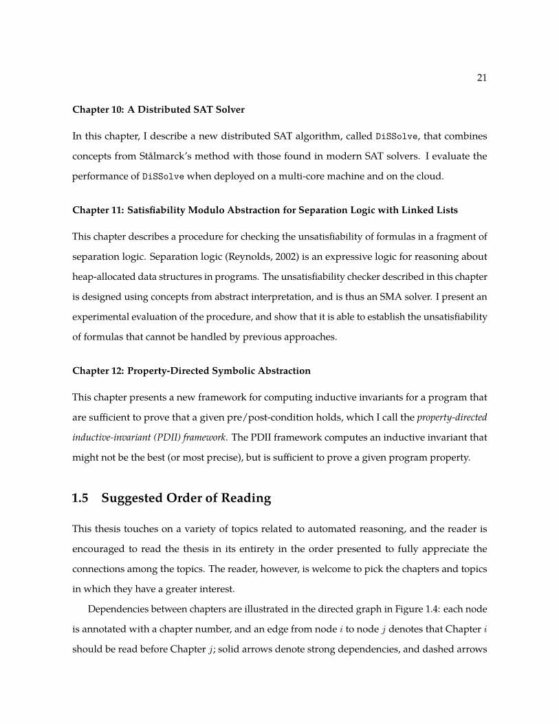
1.5 Suggested Order of Reading
This thesis touches on a variety of topics related to automated reasoning, and the reader is
encouraged to read the thesis in its entirety in the order presented to fully appreciate the
connections among the topics. The reader, however, is welcome to pick the chapters and topics
in which they have a greater interest.
Dependencies between chapters are illustrated in the directed graph in Figure 1.4: each node
is annotated with a chapter number, and an edge from node i to node j denotes that Chapter i
should be read before Chapter j; solid arrows denote strong dependencies, and dashed arrows

22
31
64
5
11
127
2
8
10
9
Figure 1.4: Dependencies among chapters
denote weak dependencies. Chapter 13, which is not shown in Figure 1.4, summarizes the results
developed during my dissertation research.
The thesis can also read in orders that follow (individually) three different threads: abstract
interpretation, decision procedures, and machine-code verification. The chapters relevant to
these three topics are listed in Table 1.1. (The results of the thesis in each of these three topics
are also summarized in Chapter 13 at a more technical level than is appropriate for the present
chapter.)
Topic Relevant chapters
Abstract Interpretation Chapters 3, 4, 5, 6, 7, 8, and 12Decision Procedures Chapters 3, 6, 10, and 11Machine-Code Verification Chapters 2, 8, and 9
Table 1.1: Chapters relevant to a particular topic

23
1.6 Chapter Notes
The beginning is always the hardest. When I started writing this thesis, I was stuck with the
question of what the first chapter should actually “introduce.” This thesis covers a wide range of
topics in automated reasoning that include theoretical results in abstract interpretation, practical
techniques for machine-code verification, decision procedures for propositional logic, and an
unsatisfiability checker for separation logic. Introducing all the problems and solution spaces
relevant to this thesis in a single chapter appeared daunting and near impossible.
I then came across an article by Karp (2011) that explores the changing relationship between
computer science and the natural and social sciences. This new relationship, referred to as the
computational lens, sees computation as a kind of lens through which to view the world of science.
This computational view enables the use of concepts of computer science to give new insights
and new ways of thinking about the physical and social sciences. Though the specific research
goals described in that article have little to do with this thesis, the title and message of the article
resonated with me: the use and benefits of viewing the physical and social sciences though the
computational lens paralleled the use and benefits of viewing program verification and decision
procedures through the abstraction lens, albeit on a more modest scale. This thought process
led to the title of this first chapter.
24
Chapter 2
There’s Plenty of Room at the Bottom
Now the name of this talk is “There is Plenty of Room at
the Bottom”—not just “There is Room at the Bottom.”— Richard Feynmann, There is Plenty of Room at the Bottom
This chapter introduces the reader to the unique opportunities and challenges involved in
analyzing machine code. Consequently, this chapter puts into context the tools and techniques
for machine-code analysis and verification developed in this thesis, especially MCVETO, the
Machine-Code VErification TOol (Chapter 9).
The purpose and contributions of the chapter can be summarized as follows:
1. I state the need for and advantages of machine-code analysis and verification (Section 2.1).
2. I state the challenges in analyzing machine code, as compared to source-code analysis
(Section 2.2).
3. I give an overview of the design space of tools and techniques for machine-code analysis
(Section 2.3).
Though applicable to a wide-range of instruction sets, the examples and instantiations used
in this thesis use the the 32-bit Intel x86 instruction set (also called IA32). For readers who
25
need a brief introduction to IA32, it has six 32-bit general-purpose registers (eax, ebx, ecx,
edx, esi, and edi), plus two additional registers: ebp, the frame pointer, and esp, the stack
pointer. By convention, register eax is used to pass back the return value from a function call.
In Intel assembly syntax, the movement of data is from right to left (e.g., mov eax,ecx sets the
value of eax to the value of ecx). Arithmetic and logical instructions are primarily two-address
instructions (e.g., add eax,ecx performs eax := eax + ecx). An operand in square brackets
denotes a dereference (e.g., if v is a local variable stored at offset -12 off the frame pointer,
mov [ebp-12],ecx performs v := ecx). Branching is carried out according to the values of
condition codes (“flags”) set by an earlier instruction. For instance, to branch to L1 when eax and
ebx are equal, one performs cmp eax,ebx, which sets ZF (the zero flag) to 1 iff eax− ebx = 0. At
a subsequent jump instruction jz L1, control is transferred to L1 if ZF = 1; otherwise, control
falls through.
2.1 The Need for Machine-Code Analysis
Traditionally, verification efforts have focused on analyzing source code. The need for investigat-
ing new techniques for performing machine-code analysis and verification can be summarized
as follows:
• In certain situations, source code is not available, and the only available artifact for analysis
is machine code.
• Machine code is an artifact that is closer to what actually executes on the machine; models
derived from machine code can be more accurate than models derived from source code.
• Analysis and verification techniques that have typically been applied to source code would
be unsound if applied to machine code.
Source code is not available when analyzing malware and viruses, or third-party libraries and
drivers. Thus, when trying to understand the behavior of malware, or trying to vet third-party
binaries for security vulnerabilities, the only option is to analyze machine code.

26
Computers do not execute source-code programs, they execute machine-code programs.
Consequently, there is a mismatch between what the programmer sees in the source code and
what is executed. Furthermore, analyses that are performed on source code can fail to detect
certain bugs and security vulnerabilities (particularly because compilation, optimization, and
link-time transformation can change how the code behaves). Balakrishnan et al. (2007) call this
phenomenon WYSINWYX for “What You See Is Not What You eXecute”.
When source code is compiled, the compiler and optimizer make certain choices that eliminate
some possible behaviors—hence there is sometimes the opportunity to obtain more precise
answers from machine-code analysis than from source-code analysis. For instance, security
exploits, such as buffer-overflow vulnerabilities, can depend on the layout of variables in memory,
which in turn depends on the idiosyncrasies of the compiler and optimizer used to generate
the machine code from the source code (Howard, 2002); security exploits could depend on the
specific libraries that are statically and dynamically linked to the program; security exploits
could depend on the (possibly malicious) instrumentation code inserted in programs subsequent
to compilation.
Often it is challenging for the programmer to understand how the compiler transforms the
source code. For instance, compilers perform optimizations that exploit undefined behavior in
programs; though perfectly sound with respect to the language semantics, such optimizations
have unexpected consequences, such as incorrect functionality and deleting security checks
(Wang et al., 2013).
The previous paragraph assumes that the compiler itself does not contain bugs. But compilers
do have bugs (Yang et al., 2011). In fact, so does the CPU (Cipra, 1995; AMD, 2012). How far
down do we go? There is plenty of room at the bottom.
2.2 The Challenges in Machine-Code Analysis
Machine-code analysis presents many new challenges. For instance, at the machine-code level,
memory is one large byte-addressable array, and an analyzer must handle computed—and
27
possibly non-aligned—addresses. It is crucial to track array accesses and updates accurately;
however, the task is complicated by the fact that arithmetic and dereferencing operations are
both pervasive and inextricably intermingled. For instance, consider the load of a local variable v,
located at offset -12 in the current activation record, into register eax: mov eax,[ebp-12]. This
instruction involves a numeric operation (ebp-12) to calculate an address whose value is then
dereferenced ([ebp-12]) to fetch the value of v, after which the value is placed in eax. Source-code
analysis tools often use separate phases of (i) points-to/alias analysis (analysis of addresses) and
(ii) analysis of arithmetic operations. Because numeric and address-dereference operations are
inextricably intertwined, as discussed above, only very imprecise information would result with
the same organization of analysis phases.
Compared with analysis of source code, the challenge is to drop all assumptions about
having certain kinds of information available (variables, control-flow graph, call-graph, etc.)
In particular, standard approaches to source-code analysis assume that certain information is
available—or at least obtainable by separate analysis phases with limited interactions between
phases—e.g.,
• a control-flow graph (CFG), or interprocedural CFG (ICFG)
• a call-graph
• a set of variables, split into disjoint sets of local and global variables
• a set of non-overlapping procedures
• type information
• points-to information or alias information
The availability of such information permits the use of techniques that can greatly aid the analysis
task. For instance, when one can assume that (i) the program’s variables can be split into (a) global
variables and (b) local variables that are encapsulated in a conceptually protected environment,
28
and (ii) a procedure’s return address is never corrupted, analyzers often tabulate and reuse
explicit summaries that characterize a procedure’s behavior.
Source-code-analysis tools sometimes also use questionable techniques, such as interpreting
operations in integer arithmetic, rather than bit-vector arithmetic. They also usually make
assumptions about the semantics that are not true at the machine-code level—for instance, they
usually assume that the area of memory beyond the top-of-stack is not part of the execution state
at all (i.e., they adopt the fiction that such memory does not exist).
Machine-code analyzers also need to address new kinds of behaviors that are not seen at the
source-code level, such as jumps to “hidden” instructions starting at positions that are out of
registration with the instruction boundaries of a given reading of an instruction stream (Linn
and Debray, 2003), and self-modifying code.
To summarize, the challenges that analysis of machine code presents include:
absence of information about variables: In stripped executables, no information is provided
about the program’s global and local variables.
a semantics based on a flat memory model: With machine code, there is no notion of separate
“protected” storage areas for the local variables of different procedure invocations, nor
any notion of protected fields of an activation record. For instance, a procedure’s return
address is stored on the stack; an analyzer must prove that it is not corrupted, or discover
what new values it could have.
absence of type information: In particular, int-valued and address-valued quantities are indis-
tinguishable at runtime.
arithmetic on addresses is used extensively: Moreover, numeric and address-dereference oper-
ations are inextricably intertwined, even during simple operations.
instruction aliasing: Programs written in instruction sets with varying-length instructions, such
as x86, can have “hidden” instructions starting at positions that are out of registration with

29
the instruction boundaries of a given reading of an instruction stream (Linn and Debray,
2003).
self-modifying code: With self-modifying code there is no fixed association between an address
and the instruction at that address.
2.3 The Design Space for Machine-Code Analysis
Machine-code-analysis problems come in at least three varieties:
1. In addition to the executable, the program’s source code is also available.
2. The source code is unavailable, but the executable includes symbol-table/debugging
information (“unstripped executables”).
3. The executable has no symbol-table/debugging information (“stripped executables”).
The appropriate variant to work with depends on the intended application. Some analysis
techniques apply to multiple variants, but other techniques are severely hampered when symbol-
table/debugging information is absent. In this thesis, I have primarily been concerned with the
analysis of stripped executables, both because it is the most challenging situation, and because
it is what is needed in the common situation where one needs to install a device driver or
commercial off-the-shelf application delivered as stripped machine code. If an individual or
company wishes to vet such programs for bugs, security vulnerabilities, or malicious code (e.g.,
back doors, time bombs, or logic bombs) analysis tools for stripped executables are required.
In this section, I describe the design space for machine-code analysis by contrasting two previ-
ous machine-code-analysis tools—CodeSurfer/x86 (Balakrishnan et al., 2005; Balakrishnan and
Reps, 2010) and DDA/x86 (Balakrishnan and Reps, 2008)—with the machine-code-verification
tool MCVETO developed in this thesis (Chapter 9). Those three tools represent several firsts:
• CodeSurfer/x86 is the first program-slicing tool for machine code that is able to track
the flow of values through memory, and thus help with understanding dependences
transmitted via memory loads and stores.

30
void foo() {int arr[2], n;void (*addr_bar)() = bar;if(MakeChoice() == 7) n = 4; // (*)else n = 2;for(int i = 0; i < n; i++)
arr[i] = (int)addr_bar; // (**)return; // can return to the entry of
bar}
void bar() {ERR:
return;}
int main() {foo();return 0;
}
Figure 2.1: A program that, on some executions, can modify the return address of foo so that fooreturns to the beginning of bar, thereby reaching ERR. (MakeChoice is a primitive that returns arandom 32-bit number.)
• DDA/x86 is the first automatic program-verification tool that is able to check whether a
stripped executable—such as a device driver—conforms to an API-usage rule (specified as
a finite-state machine).
• MCVETO is the first automatic program-verification tool capable of verifying (or detecting
flaws in) self-modifying code.
Figure 2.1 is an example that will be used to illustrate two points in the design space of
machine-code-analysis tools with respect to the question of corruption of a procedure’s return
address. When the program shown in Figure 2.1 is compiled with Visual Studio 2005, the return
address is located two 4-byte words beyond arr—in essence, at arr[3]. When MakeChoice
returns 7 at line (*), n is set to 4, and thus in the loop arr[3] is set to the starting address of
procedure bar. Consequently, the execution of foo can modify foo’s return address so that foo
returns to the beginning of bar.
In general, tools that represent different points in the design space have different answers to
the questionWhat properties are checked, and what is expected of the analyzer after the first anomalous action is
detected?First, consider the actions of a typical source-code analyzer, which would propagate abstract
states through an interprocedural control-flow graph (ICFG). The call on foo in main causes
it to begin analyzing foo. Once it is finished analyzing foo, it would follow the “return-edge”
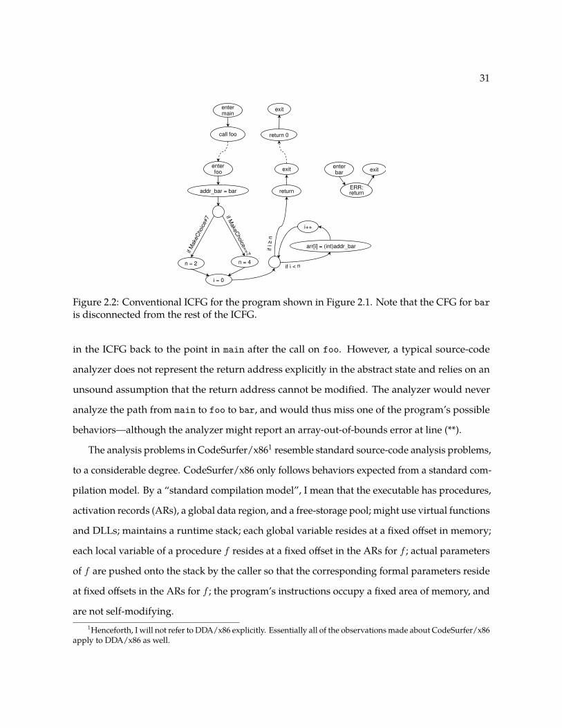
31
exit
addr_bar = bar
enterfoo
exit
entermain
return 0call foo
if Make
Choice
==7if
Make
Choic
e≠7
n = 2 n = 4
i = 0
arr[i] = (int)addr_bar
if i < nif i ≥
n
return
i++
exitenterbar
ERR:return
Figure 2.2: Conventional ICFG for the program shown in Figure 2.1. Note that the CFG for baris disconnected from the rest of the ICFG.
in the ICFG back to the point in main after the call on foo. However, a typical source-code
analyzer does not represent the return address explicitly in the abstract state and relies on an
unsound assumption that the return address cannot be modified. The analyzer would never
analyze the path from main to foo to bar, and would thus miss one of the program’s possible
behaviors—although the analyzer might report an array-out-of-bounds error at line (**).
The analysis problems in CodeSurfer/x861 resemble standard source-code analysis problems,
to a considerable degree. CodeSurfer/x86 only follows behaviors expected from a standard com-
pilation model. By a “standard compilation model”, I mean that the executable has procedures,
activation records (ARs), a global data region, and a free-storage pool; might use virtual functions
and DLLs; maintains a runtime stack; each global variable resides at a fixed offset in memory;
each local variable of a procedure f resides at a fixed offset in the ARs for f ; actual parameters
of f are pushed onto the stack by the caller so that the corresponding formal parameters reside
at fixed offsets in the ARs for f ; the program’s instructions occupy a fixed area of memory, and
are not self-modifying.1Henceforth, I will not refer to DDA/x86 explicitly. Essentially all of the observations made about CodeSurfer/x86
apply to DDA/x86 as well.

32
CodeSurfer/x86 is, however, prepared to detect and report deviations from behaviors ex-
pected from a standard compilation model, but it is not prepared to explore the consequences of
deviant behavior. When such deviations are detected, an error report is issued, and the analysis
proceeds by continuing to explore behaviors that stay within those of the desired execution
model. For instance, when the analysis discovers that the return address might be modified
within the procedure foo in Figure 2.1, CodeSurfer/x86 reports the potential violation, but
proceeds according to the original return address—i.e., by returning from foo to main. Similar
to source-code analyzers, they would not analyze the path from main to foo to bar. Although it
could miss one of the program’s possible behaviors, it reports that there is possibly an anomalous
overwrite of the return address. In the case of self-modifying code, either a write into the code
will be reported or a jump or call to data will be reported.
In contrast, MCVETO uses some techniques that permit it not only to detect the presence
of “deviant behaviors”, but also to explore them as well. The state-space-exploration method
used in MCVETO discovers that the execution of foo can modify foo’s return address. It uses
the modified return address to discover that foo actually returns to the beginning of bar, and
correctly reports that ERR is reachable. The reader is referred to Chapter 9 for more details
regarding the internals of MCVETO.
2.4 Chapter Notes
I came up with the idea for the title of this chapter when thinking of a title for an invited paper
for CAV 2010. I was rather excited about it, until Tom Reps, my adviser, mentioned that Richard
Feynman has a (famous) talk with the same title (Feynman, 1960), which I was unaware of at
the time. Tom believes I must have seen a reference to Feynman’s talk, and subconsciously
remembered it.

33
Chapter 3
Preliminaries
The advanced reader who skips parts that appear to him
too elementary may miss more than the less advanced
reader who skips parts that appear to him too complex.— G. Polya
This chapter introduces and defines concepts in (classical) abstract interpretation (Sections 3.1
and 3.1.2) and symbolic abstract interpretation (Sections 3.2.3 and 3.2.4), introduces terminology
related to decision procedures (Section 3.3), and describes Stålmarck’s method (Section 3.4).
3.1 Abstract Interpretation
Abstract interpretation (Cousot and Cousot, 1977) is a powerful framework for specifying static
program analyses. In this section, I formalize the abstract-interpretation concepts introduced in
Section 1.1. I assume familiarity with the basic concepts of abstract interpretation; a detailed
description can be found in (Nielson et al., 1999, chapter 4).
Definition 3.1. A partially ordered set (L,≤) is said to be a complete lattice if every subset M of
L has both a greatest lower bound (also called meet, denoted by M ) and a least upper bound
(also called join, denoted by⊔M ) in (L,≤). A complete lattice has a greatest element, denoted
by >, and a least element, denoted by ⊥, such that ⊥ ≤ m ≤ >, for each m ∈ L. �

34
Let (C,vC) be a complete lattice representing the concrete collecting semantics of the program.
Usually calculations using C may be too costly or even uncomputable. This situation motivates
using a simpler lattice (A,vA). The abstraction function α : C → A and the concretization function
γ : A → C are used to express the relationship between C and A. In particular, α expresses what
element of A is used to represent an element of C, and γ expresses the meaning of an element of
A in terms of an element of C.
Definition 3.2. We define G = C −−→←−−αγA to be a Galois connection between complete lattices
(C,vC) and (A,vA) if and only if α : C → A and γ : A → C are total functions that satisfy
α(c) vA a⇔ c vC γ(a) (3.1)
�
Intuitively, Equation (3.1) expresses that α and γ “respect” the orderings of the two lattices:
If an element c ∈ C is described by the element α(c) ∈ A, then all elements a ∈ A that are higher
than α(c) in the A-lattice order—α(c) vA a—should be mapped to elements γ(a) ∈ C that are
higher than c in the C-lattice order—c vC γ(a).
The next example illustrates the concepts of abstraction and concretization functions using
the abstract domain of intervals introduced in Section 1.1.
Example 3.3. Let C be the the powerset of states over integer variables x and y, and A could be
the lattice of states over intervals.
c1 ={[x 7→ 2, y 7→ 200], [x 7→ 5, y 7→ 120], [x 7→ 10, y 7→ 20]
}α(c1) = a1 =
[x 7→ [2, 10], y 7→ [20, 200]
]γ(a1) = c2 =
{[x 7→ 2, y 7→ 20], [x 7→ 2, y 7→ 21], . . . , [x 7→ 2, y 7→ 200],
[x 7→ 10, y 7→ 20], [x 7→ 10, y 7→ 21], . . . , [x 7→ 10, y 7→ 200}
The abstract value a1 = α(c1) is the interval representation of concrete states in c1 ∈ C. Notice
that there is a loss of precision when moving from C to A; however, the abstract value a1 is a

35
more succinct representation of c1. Applying the concretization function γ to the abstract value
a1 results in the set of concrete states c2. Note that c1 vC c2. �
I will make use of the following properties of a Galois connection G = C −−→←−−αγA (Nielson
et al., 1999, section 4.3.1):
• γ uniquely determines α by
α(c) ={a∣∣ c vC γ(a)
}(3.2)
• α is completely additive; that is, given C ⊆ C,
α(⊔
C)
=⊔{
α(c)∣∣ c ∈ C} (3.3)
Definition 3.4. The representation function β maps a singleton concrete state σ such that {σ} ∈ C
to the least value in A that over-approximates {σ}. �
In other words, β returns the abstraction of a singleton concrete state; i.e.,
β(σ) = α ({σ}) . (3.4)
Experience shows that, for most abstract domains, it is easy to implement a β function. Note
that implementing the α function can still be challenging, especially when a formula is used to
specify an infinite (or large) state set.
If C is the powerset of some set of states and c ∈ C, then using Equations (3.4) and (3.3) we
have that
α(c) =⊔σ∈c
β(σ) (3.5)
3.1.1 Conjunctive Abstract Domains
Many common abstract domains, and all the domains used in this thesis, fall into the category
of conjunctive domains.

36
Domain Φ
Integer Interval domain inequalities of the form c1 ≤ vand v ≤ c2 over integers
Polyhedral domain linear inequalities over reals or rationalsBit-Vector Interval domain I2w inequalities of the form c1 ≤ v
and v ≤ c2 integers mod 2wAffine-equalities domain E2w affine equalities over integers mod 2w
Table 3.1: Examples of conjunctive domains. v, vi represent program variables and c, ci representconstants
Definition 3.5. Let Φ be a given set of formulas expressed in L. A conjunctive domain over Φ is
an abstract domain A such that:
• For any a ∈ A, there exists a finite subset Ψ ⊆ Φ such that γ(a) = J∧
ΨK.
• For any finite Ψ ⊆ Φ, there exists an a ∈ A such that γ(a) = J∧
ΨK.
• There is an algorithm that, for all a1, a2 ∈ A, checks whether a1 v a2 holds. �
Table 3.1 lists the conjunctive domains used in this thesis.
The polyhedral domain and its associated abstract operations are defined in (Cousot and Halb-
wachs, 1978). An element of the polyhedral domain (Cousot and Halbwachs, 1978) is a convex
polyhedron, bounded by hyperplanes; that is, each polyhedron can be expressed as some conjunc-
tion of linear inequalities (“half-spaces”) from the set F = {∑v∈V cvv ≥ c | c, cv are constants},
where V is the set of program variables.
The affine-equalities domain E2w and its associated abstract operations are defined in Elder
et al. (2011). An element of the affine-equalities domain E2w is a set of affine equalities, where
each equality Ci is of the form Σjaijvj + bi = 0, aij , bi ∈ Z2w , vj ∈ V . In this thesis, we are
mainly interested in versions of the E2w that are based on machine arithmetic, e.g., arithmetic
modulo 28, 216, 232, or 264, and are able to take care of arithmetic overflow. The domain of
affine-equalities over integers EZ was first studied by Karr (1976). The abstract domain EZ does not
take into account overflow; consequently, the analysis results of an EZ analysis can be unsound.
Furthermore, E2w is more expressive than EZ. For instance, it is possible to express the parity of

37
a variable in E2w , but not in EZ. In arithmetic mod 2w, multiplying by a power of 2 serves to shift
bits to the left, with the effect that bits shifted off the left end are unconstrained. For example,
in E232 the affine relation 231x = 231 places a constraint solely on the least-significant bit of x;
consequently, 231x = 231 is satisfied by all states in which x is odd. Similarly, 231x = 0 is satisfied
by all states in which x is even.
3.1.2 Abstract Operations
Abstract Transformer
Suppose that G = C −−→←−−αγA is a Galois connection between concrete domain C and abstract
domainA. Then the “best transformer” (Cousot and Cousot, 1979), or best abstract post operator
for transition τ , denoted by Post[τ ] : A → A, is the most-precise abstract operator possible, given
A, for the concrete post operator for τ , Post[τ ] : C → C. Post[τ ] can be expressed in terms of α, γ,
and Post[τ ], as follows (Cousot and Cousot, 1979):
Post[τ ] = α ◦ Post[τ ] ◦ γ (3.6)
Equation (3.6) defines the limit of precision obtainable using abstraction A. However, it is
non-constructive; it does not provide an algorithm, either for applying Post[τ ] or for finding a
representation of the function Post[τ ]. In particular, in many cases, the application of γ to an
abstract value would yield an intermediate result—a set of concrete states—that is either infinite
or too large to fit in computer memory.
In practice, analysis designers typically give up on Equation (3.6) and manually write, for
each concrete operation, an abstract transformer that satisfies the weaker condition
Post][τ ] w α ◦ Post[τ ] ◦ γ. (3.7)
Furthermore, an analysis designer needs to prove that Equation (3.7) holds for the abstract
transformers that he has defined.

38
One common approach for implementing abstract transformers is via operator-by-operator
reinterpretation. The analysis developer writes a sound abstract operator—&], +], ∗], |], and
=]—for each concrete operator—&, +, ∗, |, and =, respectively. These abstract operators are used
in place of the concrete operators occurring in the term used to express the concrete transformer.
Abstract Transformers via Reinterpretation
TSL (for “ Transformer Specification Language”) (Lim and Reps, 2008, 2013), is a language and
system that uses the reinterpretation approach to automate the creation of abstract-interpretation
systems (primarily for machine-code analysis). With TSL, one specifies an instruction set’s con-
crete operational semantics by writing an interpreter using a first-order functional language.
The interpreter specifies how each instruction transforms a concrete state. To define an ab-
stract interpretation for an abstract domain A, one defines “replacement” datatypes for TSL’s
numeric/bit-vector and map datatypes, along with 42 replacement numeric/bit-vector opera-
tions, 12 replacement map-access/update operations, plus a few additional operations, such
as t, u, and widen. From such a reinterpretation of the TSL meta-language, which is extended
automatically to TSL expressions and functions, TSL creates sound over-approximating trans-
formers.
In general, such an operator-by-operator reinterpretation approach is sound, but is not
guaranteed to compute Post. Furthermore, the task of manually defining the abstract operations
can be tedious and error-prone, especially for machine code where most instructions involve
bit-wise operations. Example 1.3 illustrated that applying Post can be complex even for a single
instruction. For this example, Post[τ ](a) def= (216ebx′ = 216ecx′ + 224eax′) ∧ (224ebx′ = 224ecx′),
while the reinterpretation approach results in Post][τ ] def= 224ebx′ = 224ecx′, which is a strict
over-approximation of Post[τ ](a).
Example 3.6, given below, motivates why a technique for applying Post for a sequence of
instructions is desirable.
39
Example 3.6. Consider the two Intel x86 instructions τ1def= push 42 and τ1
def= pop eax. The
instruction τ1 pushes the value 42 onto the stack, and τ2 pops the value on top of the stack into
the register eax.
As in Example 1.3, we consider the abstract domain E232 of relational affine equalities among
32-bit registers. We would like to compute Post[τ1; τ2](a), where a = >; that is, we want to
apply the abstract transformer for the sequential composition of τ1 and τ2. One approach is
to compute the value Post[τ2](Post[τ1](a)). Post[τ1](a) def= >, because A is able to only capture
relations between registers, and is incapable of holding onto properties of values on the stack.
Consequently,
Post[τ2](Post[τ1](a)) = Post[τ2](>) = >.
In contrast,
Post[τ1; τ2](A) def= eax′ = 42. �
Examples 1.3 and 3.6 illustrate the fact that an abstract domain can be expressive enough to
capture invariants before and after a sequence of operations or instructions, but not capable of
capturing invariants at some intermediate point. As illustrated in Example 1.3, the application
of a sequence of sound abstract operations can lose precision because it is necessary to express
the intermediate result in the limited language supported by the abstract domain. Example 3.6
illustrates that a similar phenomenon holds at the level of a sequence of instructions: again, the
need to express an intermediate result in the limited language supported by the abstract domain
can cause a loss of precision.
Semantic Reduction
The semantic reduction of an abstract value A ∈ A is the lowest value, according to the lattice
order of A, that has the same concretization as that of A (Cousot and Cousot, 1979).
40
Definition 3.7. Given an abstract value A ∈ A, the semantic reduction of A, denoted by ρ(A), is
defined as:
ρ(A) def={A′ | γ(A′) = γ(A)
}�
Working with semantic reductions of abstract values often improves the overall precision of
the abstract interpretation. The use of semantic reduction in computing the reduced product
(Section 1.3.1) is one such example. Furthermore, when inferring whether a program point is
unreachable, an abstract interpreter checks whether the abstract value A at that program point
is ⊥. It is possible that A is not ⊥, but ρ(A) is ⊥.
This thesis also uses the following variant of the notion of semantic reduction, which provides
a way to refine an abstract value with respect to a formula.
Definition 3.8. Abstract value A′ is a semantic reduction of A with respect to ϕ if (i) γ(A′) ∩ JϕK =
γ(A) ∩ JϕK, and (ii) A′ v A. �
Example 3.9. Let I ≡[x 7→ [4, 100]
]be an element of the interval domain I232 , andϕ ≡ (x&1 = 1).
The semantic reduction of I with respect to ϕ is I ′ ≡[x 7→ [5, 99]
], because ϕ restricts x to be an
odd number. �
The relation between Definitions 3.7 and 3.8 is explained in Section 3.2.3.
Communication Among Abstract Domains
It is often beneficial to perform analysis using multiple abstract domains (Cousot et al., 2006).
Section 1.3.1 illustrated the concepts and issues associated with combining the results from
multiple analyses automatically.
3.2 Symbolic Abstract Interpretation
The aforementioned problems with applying γ can be side-stepped by working with symbolic
representations of sets of states (i.e., using formulas in some logic L). The use of L formulas to
41
represent sets of states is convenient because logic can also be used for specifying a language’s
concrete semantics; i.e., the concrete semantics of a transformer Post[τ ] can be stated as a formula
ϕτ ∈ L that specifies the relation between input states and output states. However, the symbolic
approach introduces a new challenge: how to bridge the gap between L and A. In particular,
we need to develop (i) concepts and algorithms to handle interconversion between formulas
of L and abstract values in A, and (ii) symbolic versions of the operations that form the core
repertoire at the heart of an abstract interpreter.
3.2.1 Moving from A to L
Definition 3.10. Given an abstract value A ∈ A, the symbolic concretization of A, denoted by γ(A),
maps A to a formula γ(A) such that A and γ(A) represent the same set of concrete states (i.e.,
γ(A) = Jγ(A)K). �
Experience shows that, for most abstract domains, it is easy to write a γ function, as illustrated
in Example 1.1.
3.2.2 Moving from L to A
Definition 3.11. Given ϕ ∈ L, the symbolic abstraction of ϕ, denoted by α(ϕ), maps ϕ to the
best value in A that over-approximates JϕK (i.e., α(ϕ) = α(JϕK)). �
In other words, α(ϕ) is the strongest consequence of ϕ expressible inA. Examples 1.2 and 1.3
illustrate the concept of α.
3.2.3 Symbolic Versions of Abstract Operations
The symbolic operations of γ and α can be used to implement the abstract operations of Sec-
tion 3.1.2.

42
Abstract Transformer
Given an abstract value a ∈ A, computing Post[τ ](a) corresponds to computing α(γ(a) ∧ ϕτ ),
where ϕτ is a formula in logic L that expresses the semantics of τ . Examples 1.2 and 1.3 illustrate
this concept.
Apart from being able to compute Post[τ ](a), it is sometimes useful to create a representation
of Post[τ ]. Some intraprocedural (Graham and Wegman, 1976) and many interprocedural (Sharir
and Pnueli, 1981; Knoop and Steffen, 1992) dataflow-analysis algorithms operate on instances
of an abstract datatype T that (i) represents a family of abstract functions (or relations), and
(ii) is closed under composition and join. By “creation of a representation of Post[τ ]”, we mean
finding the best instance in T that over-approximates Post[τ ]. α(ϕτ ) computes the best instance
in T that over-approximates Post[τ ].
Example 3.12. Consider the Intel x86 instruction τ ≡ add bh,al, which was used in Example 1.3.
The formula ϕτ (Equation (1.1)) expresses the semantics of τ . Let E232 be the abstract domain of
affine equalities over the 32-bit registers eax, ebx, ecx, eax′, ebx′, and ecx′. α(ϕτ ) computes the
representation of Post[τ ]; in particular,
α(ϕτ ) ≡ (216ebx′ = 216ebx + 224eax) ∧ (eax′ = eax) ∧ (ecx′ = ecx). �
Semantic Reduction
In symbolic abstract interpretation, Assume plays the role of the semantic-reduction operation
(Definition 3.8). Given ϕ ∈ L and A ∈ A, Assume[ϕ](A) returns the best value in A that over-
approximates the meaning of ϕ in concrete states described by A. That is, Assume[ϕ](A) equals
α(JϕK ∩ γ(A)), and can be computed as α(ϕ ∧ γ(A)
).

43
Example 3.13. Consider the scenario discussed in Example 3.9. The semantic reduction of I
with respect to ϕ is
I ′ ≡ Assume[ϕ](I)
≡ α((x&1 = 1) ∧ 4 ≤ x ∧ x ≤ 100
)≡[x 7→ [5, 99]
]�
The semantic-reduction operator ρ (Definition 3.7) can be computed using Assume: ρ(A) =
Assume[γ(A)](A).
Communication Among Abstract Domains
Suppose that there are two Galois connections G1 = C −−−→←−−−α1
γ1 A1 and G2 = C −−−→←−−−α2
γ2 A2, and one
wants to work with the reduced product of A1 and A2 (Cousot and Cousot, 1979, Section 10.1),
which I denote byA1 ?A2. The semantic reduction of a pair 〈A1, A2〉 can be performed by letting
ψ be the formula γ1(A1) ∧ γ2(A2), and creating the pair 〈α1(ψ), α2(ψ)〉. Section 1.3.1 illustrates
how symbolic abstraction can be used to compute the reduced product.
Symbolic abstraction can also be used to translate an abstract value in one abstract domain
to the best abstract value in another abstract domain. This capability would allow an abstract
interpreter to use different abstract domains for different portions of a program being analyzed.
Given A1 ∈ A1, one can find the most-precise value A2 ∈ A2 that over-approximates A1 in A2 as
follows: A2 = α2(γ1(A1)).
Notation for Over-Approximating Operators
We replace “” with “˜” to denote over-approximating operators—e.g., α(ϕ), Assume[ϕ](A),
and Post[τ ](A).
44
3.2.4 Properties of Symbolic Abstraction
In this section, I give two theorems that characterize α(ϕ) in terms of underapproximating
elements (Theorem 3.14) and in terms of overapproximating elements (Theorem 3.15). These
theorems will be used later to justify algorithms that, given ϕ, find α(ϕ) from below (Chapter 4),
from above (Chapter 6), or both (Chapter 5).
Theorem 3.14. α(ϕ) =⊔{β(S)
∣∣S |= ϕ}
Proof. By definition,
α(ϕ) = α(JϕK) (3.8)
S |= ϕ if and only if {S} ⊆ JϕK (3.9)
From Equation (3.9), we have that
JϕK =⋃{
S∣∣S |= ϕ
}(3.10)
Using Equation (3.10) in Equation (3.8), we have that
α(ϕ) = α(⋃{
S∣∣S |= ϕ
})(3.11)
Using Equation (3.5) in Equation (3.11), we have that
α(ϕ) =⊔{
β(S)∣∣S |= ϕ
}
Theorem 3.15. α(ϕ) ={a∣∣ϕ⇒ γ(a)
}Proof. By definition,
α(ϕ) = α(JϕK) (3.12)
By Equation (3.2), we have that
α(JϕK) ={a∣∣ JϕK vC γ(a)
}(3.13)

45
Using Equations (3.12) and (3.13), we have that
α(ϕ) ={a∣∣ JϕK vC γ(a)
}(3.14)
From the definition of γ, we have that
γ(a) = Jγ(a)K (3.15)
Using Equation (3.15) and from the relation between vC and⇒, we have that
JϕK vC γ(a) if and only if ϕ⇒ γ(a) (3.16)
Using Equation (3.16) in Equation (3.14), we have that
α(ϕ) ={a∣∣ϕ⇒ γ(a)
}
3.3 Decision Procedures
This section introduces basic terminology related to decision procedures.
A formula ψ is satisfiable if and only if there exists an interpretation S that makes ψ true. S is
called a model of ψ, and this fact is denoted by S |= ψ. Conversely, a formula is unsatisfiable if all
interpretations make the formula false. A formula is valid if all models make the formula true. ψ
is valid if and only if ¬ψ is unsatisfiable. A valid formula is also called a tautology.
A theory T for a signature of predicate and function symbols is a set of sentences. A formula
ψ is satisfiable modulo theory T if and only if there exists a interpretation S of the theory T such
that S |= ψ. In essence, T restricts the possible meanings of the predicate and function symbols.
Unless otherwise stated, “valid” means T -valid and “satisfiable” means T -satisfiable.
A decision procedure for a logic L is an algorithm that can determine in finite time whether or
not a given formula ψ ∈ L is satisfiable. A decision procedure for Boolean or propositional logic
is called a SAT solver. A decision procedure determining satisfiability modulo a theory is called
46
a Satisfiability Modulo Theory (SMT) solver. Note that if L is closed under negation, a decision
procedure for L-satisfiability can be used for deciding L-validity.
Most modern implementations of SAT and SMT solvers compute a satisfying model, if one
exists, when given a formula ψ. They also typically take a timeout parameter that bounds the
amount of time the implementation is allowed to spend on determining the answer. Given a
formula ψ ∈ L, we use “Model(ψ)” to denote a function that returns (i) a satisfying model S if
a decision procedure is able to determine that ψ is satisfiable (typically in a given time limit),
(ii) “None” if a decision procedure is able to determine that ψ is unsatisfiable in the given time
limit, and (iii) “TimeOut” otherwise. This terminology is used in the algorithms presented in
Chapters 4 and 5.
3.4 Stålmarck’s Method for Propositional Logic
This section describes Stålmarck’s method (Sheeran and Stålmarck, 2000), a fast validity checker
(and hence a fast SAT solver) for propositional logic.
We use 0 and 1 to denote the propositional constants false and true, respectively. Propositional
variables, negations of propositional variables, and propositional constants are referred to
collectively as literals. Stålmarck’s method manipulates formula relations, which are equivalence
relations over literals. A formula relation R will be denoted by ≡R, although we generally omit
the subscript when R is understood. We use 0 ≡ 1 to denote the universal (and contradictory)
equivalence relation {li ≡ lj | li, lj ∈ Literals}.
In this section, we review the two types of proof rules used in Stålmarck’s method with the
help of examples: (i) Example 3.16 describes the simple deductive rules, called propagation rules,
used in Stålmarck’s method, and (ii) Example 3.17 describes the Dilemma rule, a branching and
merging proof rule employed by Stålmarck’s method. The algorithm is described in Section 3.4.2.
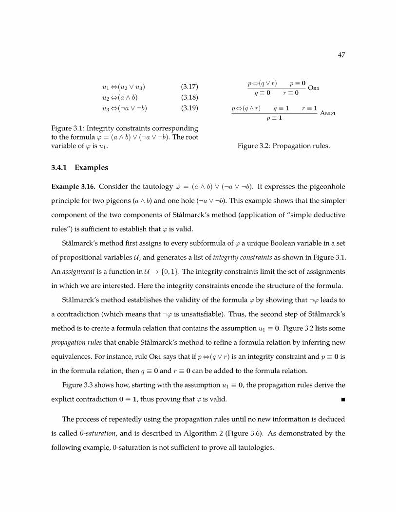
47
u1⇔(u2 ∨ u3) (3.17)u2⇔(a ∧ b) (3.18)u3⇔(¬a ∨ ¬b) (3.19)
Figure 3.1: Integrity constraints correspondingto the formula ϕ = (a ∧ b) ∨ (¬a ∨ ¬b). The rootvariable of ϕ is u1.
p⇔(q ∨ r) p ≡ 0q ≡ 0 r ≡ 0
Or1
p⇔(q ∧ r) q ≡ 1 r ≡ 1p ≡ 1
And1
Figure 3.2: Propagation rules.
3.4.1 Examples
Example 3.16. Consider the tautology ϕ = (a ∧ b) ∨ (¬a ∨ ¬b). It expresses the pigeonhole
principle for two pigeons (a ∧ b) and one hole (¬a ∨ ¬b). This example shows that the simpler
component of the two components of Stålmarck’s method (application of “simple deductive
rules”) is sufficient to establish that ϕ is valid.
Stålmarck’s method first assigns to every subformula of ϕ a unique Boolean variable in a set
of propositional variables U , and generates a list of integrity constraints as shown in Figure 3.1.
An assignment is a function in U → {0, 1}. The integrity constraints limit the set of assignments
in which we are interested. Here the integrity constraints encode the structure of the formula.
Stålmarck’s method establishes the validity of the formula ϕ by showing that ¬ϕ leads to
a contradiction (which means that ¬ϕ is unsatisfiable). Thus, the second step of Stålmarck’s
method is to create a formula relation that contains the assumption u1 ≡ 0. Figure 3.2 lists some
propagation rules that enable Stålmarck’s method to refine a formula relation by inferring new
equivalences. For instance, rule Or1 says that if p⇔(q ∨ r) is an integrity constraint and p ≡ 0 is
in the formula relation, then q ≡ 0 and r ≡ 0 can be added to the formula relation.
Figure 3.3 shows how, starting with the assumption u1 ≡ 0, the propagation rules derive the
explicit contradiction 0 ≡ 1, thus proving that ϕ is valid. �
The process of repeatedly using the propagation rules until no new information is deduced
is called 0-saturation, and is described in Algorithm 2 (Figure 3.6). As demonstrated by the
following example, 0-saturation is not sufficient to prove all tautologies.
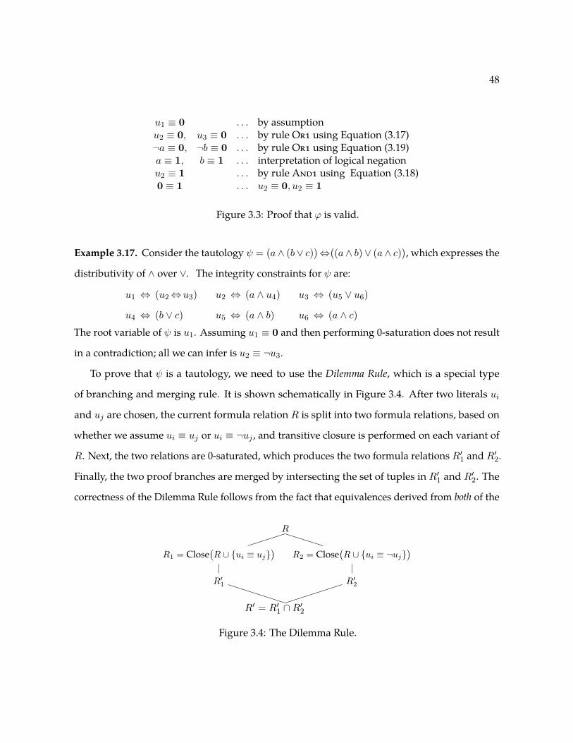
48
u1 ≡ 0 . . . by assumptionu2 ≡ 0, u3 ≡ 0 . . . by rule Or1 using Equation (3.17)¬a ≡ 0, ¬b ≡ 0 . . . by rule Or1 using Equation (3.19)a ≡ 1, b ≡ 1 . . . interpretation of logical negationu2 ≡ 1 . . . by rule And1 using Equation (3.18)0 ≡ 1 . . . u2 ≡ 0, u2 ≡ 1
Figure 3.3: Proof that ϕ is valid.
Example 3.17. Consider the tautology ψ =(a∧ (b∨ c)
)⇔((a∧ b)∨ (a∧ c)
), which expresses the
distributivity of ∧ over ∨. The integrity constraints for ψ are:
u1 ⇔ (u2⇔u3) u2 ⇔ (a ∧ u4) u3 ⇔ (u5 ∨ u6)
u4 ⇔ (b ∨ c) u5 ⇔ (a ∧ b) u6 ⇔ (a ∧ c)The root variable of ψ is u1. Assuming u1 ≡ 0 and then performing 0-saturation does not result
in a contradiction; all we can infer is u2 ≡ ¬u3.
To prove that ψ is a tautology, we need to use the Dilemma Rule, which is a special type
of branching and merging rule. It is shown schematically in Figure 3.4. After two literals ui
and uj are chosen, the current formula relation R is split into two formula relations, based on
whether we assume ui ≡ uj or ui ≡ ¬uj , and transitive closure is performed on each variant of
R. Next, the two relations are 0-saturated, which produces the two formula relations R′1 and R′2.
Finally, the two proof branches are merged by intersecting the set of tuples in R′1 and R′2. The
correctness of the Dilemma Rule follows from the fact that equivalences derived from both of the
R
R1 = Close(R ∪ {ui ≡ uj}
)R2 = Close
(R ∪ {ui ≡ ¬uj}
)R′
1 R′2
R′ = R′1 ∩R′2
Figure 3.4: The Dilemma Rule.
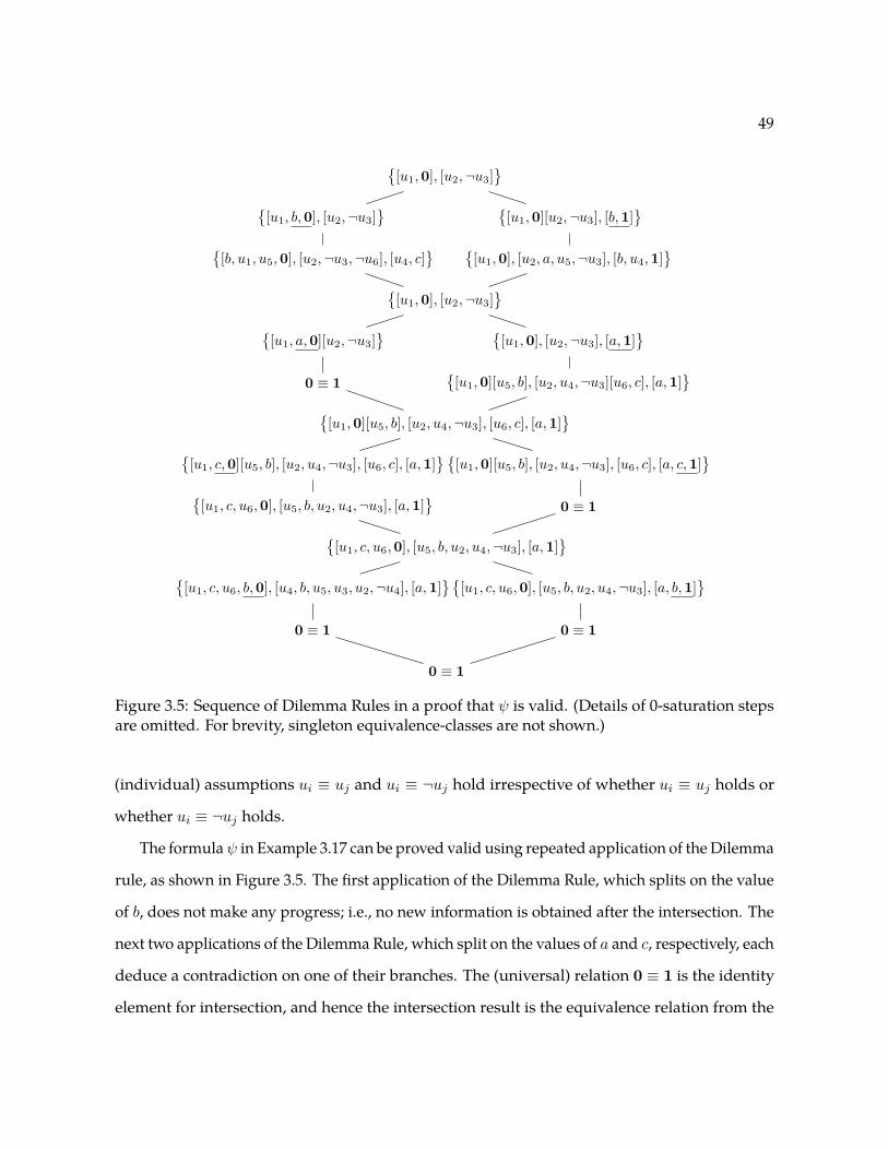
49
{[u1,0], [u2,¬u3]
}{
[u1, b,0], [u2,¬u3]} {
[u1,0][u2,¬u3], [b,1]}
{[b, u1, u5,0], [u2,¬u3,¬u6], [u4, c]
} {[u1,0], [u2, a, u5,¬u3], [b, u4,1]
}{
[u1,0], [u2,¬u3]}
{[u1, a,0][u2,¬u3]
} {[u1,0], [u2,¬u3], [a,1]
}0 ≡ 1
{[u1,0][u5, b], [u2, u4,¬u3][u6, c], [a,1]
}{
[u1,0][u5, b], [u2, u4,¬u3], [u6, c], [a,1]}
{[u1, c,0][u5, b], [u2, u4,¬u3], [u6, c], [a,1]
} {[u1,0][u5, b], [u2, u4,¬u3], [u6, c], [a, c,1]
}{
[u1, c, u6,0], [u5, b, u2, u4,¬u3], [a,1]}
0 ≡ 1
{[u1, c, u6,0], [u5, b, u2, u4,¬u3], [a,1]
}{
[u1, c, u6, b,0], [u4, b, u5, u3, u2,¬u4], [a,1]}{
[u1, c, u6,0], [u5, b, u2, u4,¬u3], [a, b,1]}
0 ≡ 1 0 ≡ 1
0 ≡ 1
Figure 3.5: Sequence of Dilemma Rules in a proof that ψ is valid. (Details of 0-saturation stepsare omitted. For brevity, singleton equivalence-classes are not shown.)
(individual) assumptions ui ≡ uj and ui ≡ ¬uj hold irrespective of whether ui ≡ uj holds or
whether ui ≡ ¬uj holds.
The formulaψ in Example 3.17 can be proved valid using repeated application of the Dilemma
rule, as shown in Figure 3.5. The first application of the Dilemma Rule, which splits on the value
of b, does not make any progress; i.e., no new information is obtained after the intersection. The
next two applications of the Dilemma Rule, which split on the values of a and c, respectively, each
deduce a contradiction on one of their branches. The (universal) relation 0 ≡ 1 is the identity
element for intersection, and hence the intersection result is the equivalence relation from the

50
Algorithm 1: propagate(J,R1, R, I)1 R2 = ApplyRule[I](J,R1)2 return Close(R ∪R2)
Algorithm 2: 0-saturation(R, I)1 repeat2 R′ ← R3 foreach J ∈ I,R1 ⊆ R do4 R← propagate(J,R1, R, I)5 until (R = R′) ‖ contradiction(R)6 return R
Algorithm 3: 1-saturation(R, I)1 repeat2 R′ ← R3 foreach vi, vj such that vi ≡ vj 6∈ R andvi ≡ ¬vj 6∈ R do
4 R1 ← Close(R ∪ {vi ≡ vj})5 R2 ← Close(R ∪ {vi ≡ ¬vj})6 R′1 ← 0-saturation(R1)7 R′2 ← 0-saturation(R2)8 R← R′1 ∩R′29 until (R = R′) ‖ contradiction(R)
10 return R
Algorithm 4: k-saturation(R, I)1 repeat2 R′ ← R3 foreach vi, vj such that vi ≡ vj 6∈ R andvi ≡ ¬vj 6∈ R do
4 R1 ← Close(R ∪ {vi ≡ vj})5 R2 ← Close(R ∪ {vi ≡ ¬vj})6 R′1 ← (k–1)-saturation(R1, I)7 R′2 ← (k–1)-saturation(R2, I)8 R← R′1 ∩R′29 until (R = R′) ‖ contradiction(R)
10 return R
Algorithm 5: k-Staalmarck(ϕ)1 (vϕ, I)← integrity(ϕ)2 R← {vϕ ≡ 0}3 R′ ← k-saturation(R, I)4 if R′ = 0 ≡ 1 then return valid5
6 else return unknown7
Figure 3.6: Stålmarck’s method. The operation Close performs transitive closure on a formularelation after new tuples are added to the relation.
non-contradictory branch. Finally, splitting on the variable b leads to a contradiction on both
branches. �
Repeatedly applying the Dilemma rule until no new information is deduced is called 1-
saturation, and is described in Algorithm 3 (Figure 3.6). Unfortunately, 1-saturation may not
be sufficient to prove certain tautologies. The 1-saturation procedure can be generalized to the
k-saturation procedure shown in Algorithm 4 (Figure 3.6).

51
3.4.2 Pseudo-Code for Stålmarck’s Method
Algorithm 1 (Figure 3.6) implements the propagation rules of Figure 3.2. Given an integrity
constraint J ∈ I and a set of equivalences R1 ⊆ R, line 1 calls the function ApplyRule, which
instantiates and applies the derivation rules of Figure 3.2 and returns the deduced equivalences in
R2. The new equivalences inR2 are incorporated intoR and the transitive closure of the resulting
equivalence relation is returned. We implicitly assume that if Close derives a contradiction then
it returns 0 ≡ 1.
Algorithm 2 (Figure 3.6) describes 0-saturation, which calls propagate repeatedly until no
new information is deduced, or a contradiction is derived. If a contradiction is derived, then the
given formula is proved to be valid.
The Dilemma Rule is applied repeatedly until no new information is deduced by a process
called 1-saturation, shown in Algorithm 3 (Figure 3.6). 1-saturation uses two literals vi and vj ,
and splits the formula relation with respect to vi ≡ vj and vi ≡ ¬vj (lines 4 and 5). 1-saturation
finds a contradiction when both 0-saturation branches identify contradictions (in which case
R = R′1 ∩R′2 equals 0 ≡ 1).
The 1-saturation procedure can be generalized to the k-saturation procedure shown in
Algorithm 4. Stålmarck’s method (Algorithm 5) is structured as a procedure for validity checking.
The actions of the algorithm are parameterized by a certain parameter k that is fixed by the user.
For a given tautology, if k is large enough Stålmarck’s method can prove validity, but if k is too
small the answer returned is “unknown”. In the latter case, one can increment k and try again.
However, for each k, (k + 1)-saturation is significantly more expensive than k-saturation: the
running time of Algorithm 5 as a function of k is O(|ϕ|k) (Sheeran and Stålmarck, 2000).
3.5 Chapter Notes
This chapter omits discussion of algorithms to compute fixpoints; the reader if referred to sections
2.4 and 4.2 of Nielson et al. (1999). Reps et al. (2007) discuss the use of weighted pushdown
systems (WPDSs) to perform inter-procedural analysis of programs. The WALi library (Kidd

52
et al., 2007) implements such a WPDS-based framework. The various analyses described in this
thesis are implemented using the WALi library.
Stålmarck’s method was protected by Swedish, European, and U.S. patents (Stålmarck, 1989),
which may have discouraged experimentation by researchers. Indeed, one finds relatively few
publications that concern Stålmarck’s method—some of the exceptions being Harrison (1996);
Cook and Gonthier (2005); Björk (2009). Kunz and Pradhan (1994) discuss an algorithm closely
related to Stålmarck’s method.
More information on SAT solvers can be found in (Harrison, 2009, Chapter 2); (Kroening and
Strichman, 2008, Chapter 2); Darwiche and Pipatsrisawat (2009); and Marques-Silva et al. (2009).
More information on SMT solvers can be found in (Kroening and Strichman, 2008, Chapters 3–7);
and Barrett et al. (2009).
53
Chapter 4
Symbolic Abstraction from Below
Started from the bottom, now we are here,
Started from the bottom, now the whole team here.— Drake
In this chapter, I review two prior algorithms for performing symbolic abstraction:
• The RSY algorithm: a framework for computing α that applies to any logic and abstract
domain that satisfies certain conditions (Reps et al., 2004).
• The KS algorithm: an algorithm for computing α that applies to QFBV logic and the
domain E2w of affine equalities. King and Søndergaard (2010) gave a specific α algorithm
for an abstract domain of Boolean affine relations. Elder et al. (2011) extended the King
and Søndergaard algorithm to the affine-equalities domain E2w . Because the generalized
algorithm is similar to the Boolean one, we refer to it as KS.
I also present the results of an experiment I carried out to compare the performance of the
two algorithms. Both algorithms compute α(ϕ) via successive approximation from “below”,
computing a sequence of successively “larger” approximations to the set of states described by ϕ.

54
Algorithm 6: α↑RSY〈L,A〉(ϕ)1 lower← ⊥2
3 while true do4
5 S ← Model(ϕ ∧ ¬γ( lower))6 if S is TimeOut then7 return >8 else if S is None then9 break // ϕ⇒ γ(lower)
10 else // S 6|= γ(lower)11 lower← lower t β(S)12 ans← lower13 return ans
Algorithm 7: α↑KS(ϕ)1 lower← ⊥2 i← 13 while i ≤ rows(lower) do4 p← Row(lower,−i) // p w lower5 S ← Model(ϕ ∧ ¬γ(p))6 if S is TimeOut then7 return >8 else if S is None then9 i← i+ 1 // ϕ⇒ γ(p)
10 else // S 6|= γ(p)11 lower← lower t β(S)12 ans← lower13 return ans
The purpose and contributions of this chapter can be summarized as follows:
1. To present algorithms for performing symbolic abstraction that are representative of the
state-of-the-art prior to this thesis (Sections 4.1 and 4.2).
2. To present the RSY and KS algorithms in a common setting (Algorithms 6 and 7).
3. To present an empirical comparison of the RSY and KS algorithms (Section 4.3).
The results of item 3 served as motivation for the new algorithms that I developed, described
in Chapters 5 and 6.
4.1 RSY Algorithm
Reps et al. (2004) presented a framework for computing α—which we call the RSY algorithm—
that applies to any logic L and abstract domain A that satisfy certain conditions. The key insight
of the algorithm is the use an SMT solver for L as a black-box to query for models of ϕ. Recall
the following property of α (Theorem 3.14):
α(ϕ) =⊔{
β(S)∣∣S |= ϕ
}(4.1)
55
Equation (4.1) states that α(ϕ) is the result of performing a join of the abstraction of models
of ϕ. Unfortunately, Equation (4.1) does not directly lead to an algorithm for computing α(ϕ),
because, as stated, it involves finding all models of ϕ, which would be impractical. The RSY
algorithm does not find all models of ϕ; instead the algorithm queries the SMT solver to compute
a finite sequence S1, S2, . . . , Sk−1, Sk of models of ϕ. This sequence of models is used to compute
a sequence of abstract values A0, A1, A2, . . . , Ak−1, Ak in the following way:
A0 = ⊥ (4.2)
Ai = Ai−1 t β(Si), Si |= ϕ, 1 ≤ i ≤ k (4.3)
Merely sampling k arbitrary models of ϕ would not work. In particular, it is possible that
Ai−1 = Ai in Equation (4.3) in which case step i has not made progress. Thus, to ensure progress
we require Si to be a model of ϕ such that Si /∈ γ(Ai−1) in Equation (4.3). In other words, Si
should be a model satisfying ϕ ∧ ¬γ(Ai−1). Computing Si in such a way ensures that Ai−1 Ĺ Ai
in Equation (4.3). Equations (4.2) and (4.3) can be restated as:
A0 = ⊥ (4.4)
Ai = Ai−1 t β(Si), Si |= ϕ ∧ ¬γ(Ai−1), 1 ≤ i ≤ k (4.5)
Furthermore, provided the abstract domain A has no infinite ascending chains, there exists a k
such that Ak = α(ϕ), because each step is guaranteed to make progress up the lattice. That is,
using Equations (4.4) and (4.5), we can construct a finite sequence of abstract values that form an
ascending chain that converges to α(ϕ):
⊥ = A0 @ A1 @ A2 @ . . . @ Ak−1 @ Ak = α(ϕ). (4.6)
Algorithm 6 shows the general RSY algorithm: α↑RSY〈L,A〉 is parameterized on logic L and
abstract domain A. The algorithm assumes there is a decision procedure for logic L, and uses
notation introduced in Section 3.3.

56
The algorithm implements Equations (4.4) and (4.5): the algorithm maintains an under-
approximation of the final answer in the variable lower, which is initialized to ⊥ on line 1, and
updated by performing a join (line 11). γ(lower) is used as a “blocking clause”, and thus the
model S of ϕ returned on line 5 is one that is not already represented by lower (i.e., S is not in
the concretization of lower). Consequently, lower Ĺ lower t β(S), and the updated value of lower
on line 11 is a strictly larger approximation to the set of states described by ϕ. Thus, provided
the abstract domainA has no infinite ascending chains, Algorithm 6 eventually terminates when
the call to Model on line 5 returns None. In this case, lower = α(ϕ).
Note that if the call to Model returns TimeOut, then Algorithm 6 returns > (line 6), which is a
trivial, but sound, over-approximation of α(ϕ). In other words, the RSY algorithm implements
α(ϕ); however, if in a given run of the algorithm there is no timeout, the value returned equals
α(ϕ). In this sense, all of the algorithms described in the thesis are implementations of α.
By looking at the pseudo-code in Algorithm 6, we can determine the assumptions on the
logic and the abstract domain made by the RSY algorithm:
1. There is a Galois connection C −−→←−−αγA between A and concrete domain C, and an imple-
mentation of the corresponding representation function β (see line 11).
2. There is an algorithm to evaluate a1 t a2 for all a1, a2 ∈ A (see line 11).
3. There is a symbolic-concretization operation γ that maps an abstract value a ∈ A to a
formula γ(a) in L (see line 5).
4. A has no infinite ascending chains.
5. There is a decision procedure for the logic L that is also capable of returning a model
satisfying a formula in L (see line 5).
6. The logic L is closed under conjunction and negation (see line 5).
I omit the formal proof of the correctness of the algorithm. The proof can be found in Reps
et al. (2004). Furthermore, the correctness of Bilateral algorithm, which is a generalization of the
RSY algorithm, will be given in Chapter 5.

57
Algorithm 8: Post↑[τ ](v)
1 lower′ ← ⊥2 while true do3 〈S, S′〉 ← Model(γ(v) ∧ ϕτ ∧ ¬γ(lower′))4 if 〈S, S′〉 is TimeOut then5 return >6 else if 〈S, S′〉 is None then7 break // Post[τ ](v) = lower′
8 else // S′ 6|= γ(lower′)9 lower′ ← lower′ t β(S′)
10 v′ ← lower′11 return v’
4.1.1 Computing Post
Algorithm 6, which computes the symbolic abstraction of a formula, can be adapted to compute
Post for a concrete transformer τ and input abstract value a ∈ A. Recall that Post satisfies
Post[τ ](a) = (α ◦ Post[τ ] ◦ γ)(a). Algorithm 8 shows the algorithm that computes Post.
ϕτ represents the formula in logic L that captures the input-output relation for the concrete
transformer τ . The main difference between Algorithm 6 and Algorithm 8 is call to Model on
line 3. Algorithm 8 will be used in Chapter 7.
4.2 KS Algorithm
Algorithm 7 presents the α↑KS algorithm for computing α that applies to the QFBV logic and
affine-equalities domain E2w . King and Søndergaard (2010) first presented the algorithm for
abstract domain for Boolean affine relations, which was generalized to the domain of affine
equalities by Elder et al. (2011).
An abstract value in the E2w domain is a conjunction of affine equalities, which can be
represented in a normal form as a matrix in which each row expresses a non-redundant affine
equality (Elder et al., 2011). (Rows are 0-indexed.) Given a matrixm, rows(m) returns the number
of rows of m (as in line 3 in Algorithm 7 ), and Row(m,−i), for 1 ≤ i ≤ rows(m), returns row
(rows(m)− i) of m (as in line 4 in Algorithm 7).

58
The presentation in Algorithm 7 differs significantly from that in (King and Søndergaard,
2010, figure 2); in particular, Algorithm 7 is stated using the terminology of symbolic abstract
interpretation (Section 3.2.3). The similarities between the RSY algorithm (Algorithm 6) and the
KS algorithm are easier to see in this presentation. Both algorithms have a similar overall structure.
Both are successive approximation algorithms: they compute a sequence of successively “larger”
approximations to the set of states described by ϕ. Both maintain an under-approximation of
the final answer in the variable lower, which is initialized to ⊥ on line 1. Both call a decision
procedure (line 5), and if a model S is found that satisfies the query, the under-approximation is
updated by performing a join (line 11).
The RSY and KS algorithms have a similar overall structures (Algorithms 6 and 7). The
differences between Algorithms 6 and 7 are highlighted in gray. The key difference is the nature
of the decision-procedure query on line 5. α↑RSY uses all of lower to construct the query, while
α↑KS uses only a single row from lower (line 4)—i.e., just a single affine equality, which has two
consequences. First, α↑KS should issue a larger number of queries than α↑RSY, for the following
reason. Suppose that the value of lower has converged to the final answer via a sequence of joins
performed by the algorithm. To discover that convergence has occurred, α↑RSY has to issue just a
single decision-procedure query, whereas α↑KS has to confirm it by issuing rows(lower)−i number
of queries, proceeding row-by-row. Second, each individual query issued by α↑KS is simpler than
the ones issued by α↑RSY. Thus, a priori, it is not clear which algorithm will perform better in
practice; an empirical comparison of the RSY and KS algorithms is provided in Section 4.3.
I omit the formal proof of the correctness of the KS algorithm. The proof can be found in
Elder et al. (2014). Furthermore, the correctness of Bilateral algorithm, which is a generalization
of the KS algorithm, will be given in Chapter 5.
4.3 Empirical Comparison of the RSY and KS Algorithms
In this section, I provide an quantitative comparison of the performance of the KS algorithm
and the RSY framework instantiated for the affine-equalities domain E232 . We use RSY[E232 ] to

59
name instrs procs BBs brs
finger 532 18 298 48subst 1093 16 609 74label 1167 16 573 103chkdsk 1468 18 787 119convert 1927 38 1013 161route 1982 40 931 243logoff 2470 46 1145 306setup 4751 67 1862 589
Table 4.1: The characteristics of the x86 binaries of Windows utilities used in the experiments.The columns show the number of instructions (instrs); the number of procedures (procs); thenumber of basic blocks (BBs); the number of branch instructions (brs).
Figure 4.1: Total time taken by all invocations of α↑RSY[E232 ] compared to that taken by α↑KS foreach of the benchmark executables. The running time is normalized to the corresponding timetaken by α↑RSY[E232 ]; lower numbers are better.
denote the RSY framework instantiated for the affine-equalities domain E232 .
The experiments in this section were designed to answer the following questions:
1. How does the speed of α↑KS compare with that of α↑RSY[E232 ]?
2. What are the reasons for the differences between the running times of α↑KS and α↑RSY[E232 ]?
To address these questions, we performed affine-relations analysis (ARA) on x86 machine
code, computing affine relations over the x86 registers. Our experiments were run on a single

60
(a) (b)
Figure 4.2: (a) Scatter plot showing of the number of decision-procedure queries during eachpair of invocations of α↑RSY and α↑KS, when neither invocation had a decision-procedure timeout.(b) Log-log scatter plot showing the times taken by each pair of invocations of α↑RSY and α↑KS,when neither invocation had a decision-procedure timeout.
core of a quad-core 3.0 GHz Xeon computer running 64-bit Windows XP (SP2), configured so
that a user process has 4GB of memory. We analyzed a corpus of Windows utilities (Table 4.1)
using the WALi (Kidd et al., 2007) system for weighted pushdown systems (WPDSs). 1 For the
α↑KS-based (α↑RSY-based) analysis we used a weight domain of α↑KS-generated (α↑RSY-generated)
ARA transformers. The weight on each WPDS rule encodes the ARA transformer for a basic block
B of the program, including a jump or branch to a successor block. A formula ϕB is created that
captures the concrete semantics of B, and then the ARA weight for B is obtained by performing
α(ϕB). We compared the time for α↑RSY[E232 ] and α↑KS to compute basic-block transformers for this
set of x86 executables. There was no overall timeout imposed on the invocation of the procedures,
but each invocation of the decision procedure (line 5 in Algorithms 6 and 7) had a timeout of 31Due to the high cost of the ARA-based WPDS construction, all analyses excluded the code for libraries. Because
register eax holds the return value from a call, library functions were modeled approximately (albeit unsoundly, ingeneral) by “havoc(eax)”.
61
seconds (as in Elder et al. (2011)).
Figure 4.1 shows the total time taken by all invocations of α↑RSY compared to that taken by α↑KS
for each of the benchmark executables. The running time is normalized to the corresponding
time taken by α↑RSY; lower numbers are better. Overall, α↑KS is about ten times faster compared to
α↑RSY; this answers the question posed in item 1 above.
Figure 4.2(a) shows a scatter-plot of the number of decision-procedure calls in each invocation of
α↑RSY versus the corresponding invocation of α↑KS, when neither of the procedures had a decision-
procedure timeout. α↑RSY issues fewer decision-procedure queries: on average (computed as an
arithmetic mean), α↑KS invokes 42% more calls to the decision procedure. Figure 4.2(b) shows a
log-log scatter-plot of the total time taken by each invocation of α↑RSY versus the time taken by
α↑KS. α↑KS is much faster than α↑RSY: overall, computed as the geometric mean of the speedups on
each of the x86 executables, α↑KS is about ten times faster compared to α↑RSY[E232 ].
The order-of-magnitude speedup can be attributed to the fact that each of the α↑KS decision-
procedure queries is less expensive than the ones issued by α↑RSY even though α↑KS issues more
decision-procedure calls. At line 4 in α↑KS, p is a single constraint; consequently, the decision-
procedure query contains the single conjunct ¬γ(p) (line 5). In contrast, at line 5 in α↑RSY, lower is
a conjunction of constraints, and consequently the decision-procedure query contains ¬γ(lower),
which is a disjunction of constraints.

62
Chapter 5
A Bilateral Algorithm for Symbolic
Abstraction
Great results can be achieved with small forces.
— Sun Tzu, The Art of War
In this chapter, I use the insights gained from the algorithms presented in Chapter 4 to design
a new framework for symbolic abstraction that
• is parametric and is applicable to any abstract domain that satisfies certain conditions
(similar to the RSY algorithm)
• uses a successive-approximation algorithm that is parsimonious in its use of the decision
procedure (similar to the KS algorithm)
• is bilateral; that is, it maintains both an under-approximation and a (non-trivial) over-
approximation of the desired answer, and hence is resilient to timeouts: the procedure
can return the over-approximation if it is stopped at any point (unlike the RSY and KS
algorithms).
In contrast, neither the RSY algorithm nor KS algorithm is resilient to timeouts. A decision-
procedure query—or the cumulative time for α↑—might take too long, in which case the only
safe answer that can be returned is > (line 6 in Algorithms 6 and 7).

63
Algorithm Parametric Resilient Parsimonious
RSY (Section 4.1) 3 7 7
KS (Section 4.2) 7 7 3
Bilateral (Section 5.2) 3 3 3
Table 5.1: Qualitative comparison of symbolic-abstraction algorithms. A 3 indicates that thealgorithm has a property described by a column, and a 7 indicates that the algorithm does nothave the property.
Table 5.1 compares the features of the various algorithms for symbolic abstraction. Thus,
the Bilateral algorithm combines the best features of the KS and RSY algorithms, but also has
benefits that none of these previous algorithms have.
The contributions of this chapter can be summarized as follows:
• I show how the KS algorithm can be modified into the KS+ algorithm, which maintains
sound under- and over-approximations of the answer (Section 5.1).
• I present a framework for symbolic abstraction based on a bilateral algorithm for computing
α (Section 5.2).
• I extend the bilateral algorithm to handle abstract domains with infinite descending chains
(Section 5.3).
• I give several instantiations of the bilateral framework (Section 5.4).
• I compare the performance of the KS algorithm and an instantiation of the Bilateral frame-
work (Section 5.5).
Section 5.6 describes a Bilateral algorithm for computing Post. Section 5.7 presents related work.
5.1 Towards a Bilateral Algorithm
In this section, I describe how the KS algorithm (Algorithm 7) can be made resilient to timeouts.
In particular, I show how α↑KS can be modified to maintain a non-trivial over-approximation

64
Algorithm 9: α↑KS(ϕ)1
2 lower← ⊥3 i← 14 while i ≤ rows(lower) do5 p← Row(lower,−i)// p w lower
6 S ← Model(ϕ ∧ ¬γ(p))7 if S is TimeOut then8 return >9 else if S is None then
// ϕ⇒ γ(p)10 i← i+ 111 else // S 6|= γ(p)12 lower← lower t β(S)13 ans← lower14 return ans
Algorithm 10: αlKS+(ϕ)
1 upper← >2 lower← ⊥3 i← 14 while i ≤ rows(lower) do5 p← Row(lower,−i)// p w lower, p 6w upper
6 S ← Model(ϕ ∧ ¬γ(p))7 if S is TimeOut then8 return upper9 else if S is None then
10 upper← upper u p // ϕ⇒ γ(p) i← i+ 111 else // S 6|= γ(p)12 lower← lower t β(S)13 ans← lower14 return ans
of the desired answer. Algorithm 10 is thus a bilateral algorithm: it maintains both an under-
approximation and over-approximation of α(ϕ). The original α↑KS is shown in Algorithm 9 for
comparison; the differences in the algorithms are highlighted in gray. (Note that line numbers
are different in Algorithms 7 and 9.)
The αlKS+ algorithm (Algorithm 10) initializes the over-approximation (upper) to > on line 1.
At any stage in the algorithm ϕ⇒ γ(upper). On line 10, it is sound to update upper by performing
a meet with p because ϕ⇒ γ(p). Progress is guaranteed because p 6w upper. In case of a decision-
procedure timeout (line 7), Algorithm 10 returns upper as the answer (line 8). Thus, αlKS+(ϕ) can
return a non-trivial over-approximation of α(ϕ) in case of a timeout. However, if the loop exits
without a timeout, then αlKS+(ϕ) returns α(ϕ).
5.2 A Parametric Bilateral Algorithm
Like the original KS algorithm, αlKS+ applies only to the affine-equalities domain E2w . The results
presented in Section 4.3 provide motivation to generalize αlKS+ so that we can take advantage
of its benefits with domains other than E2w . In this section, I present the bilateral framework,

65
which applies to any abstract domain that satisfies the interface defined below. (Note that the
interface for the Bilateral framework is slightly different than the interface for the RSY framework
presented in Section 4.1.)
I first introduce the abstract-consequence operation, which is the key operation in our general-
ized algorithm:
Definition 5.1. An operation AbstractConsequence(·, ·) is an acceptable abstract-consequence oper-
ation iff for all a1, a2 ∈ A such that a1 Ĺ a2,
a = AbstractConsequence(a1, a2) implies a1 v a and a 6w a2. �
Figure 5.1 illustrates Definition 5.1 graphically, using the concretizations of a1, a2, and a.
Algorithm 11 presents the parametric bilateral algorithm αl〈L,A〉(ϕ), which performs sym-
bolic abstraction of ϕ ∈ L for abstract domain A. The differences between Algorithms 11 and 10
are highlighted in gray.
The assumptions placed on the logic and the abstract domain are as follows:
1. There is a Galois connection C −−→←−−αγA between A and concrete domain C, and an imple-
mentation of the corresponding representation function β.
2. Given a1, a2 ∈ A, there are algorithms to evaluate a1 t a2 and a1 u a2, and to check a1 = a2.
3. There is a symbolic-concretization operation γ that maps an abstract value a ∈ A to a
formula γ(a) in L.
Figure 5.1: Abstract Consequence: For all a1, a2 ∈ A where γ(a1) ( γ(a2), if a =AbstractConsequence(a1, a2), then γ(a1) ⊆ γ(a) and γ(a) 6⊇ γ(a2).
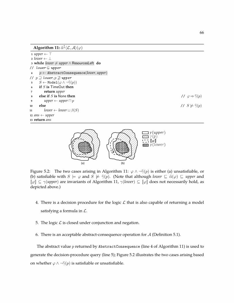
66
Algorithm 11: αl〈L,A〉(ϕ)1 upper← >2 lower← ⊥3 while lower 6= upper ∧ ResourcesLeft do
// lower Ĺ upper4 p← AbstractConsequence(lower,upper)
// p w lower, p 6w upper5 S ← Model(ϕ ∧ ¬γ(p))6 if S is TimeOut then7 return upper8 else if S is None then // ϕ⇒ γ(p)9 upper← upper u p
10 else // S 6|= γ(p)11 lower← lower t β(S)12 ans← upper13 return ans
S
(b)(a)
Figure 5.2: The two cases arising in Algorithm 11: ϕ ∧ ¬γ(p) is either (a) unsatisfiable, or(b) satisfiable with S |= ϕ and S 6|= γ(p). (Note that although lower v α(ϕ) v upper andJϕK ⊆ γ(upper) are invariants of Algorithm 11, γ(lower) ⊆ JϕK does not necessarily hold, asdepicted above.)
4. There is a decision procedure for the logic L that is also capable of returning a model
satisfying a formula in L.
5. The logic L is closed under conjunction and negation.
6. There is an acceptable abstract-consequence operation for A (Definition 5.1).
The abstract value p returned by AbstractConsequence (line 4 of Algorithm 11) is used to
generate the decision-procedure query (line 5); Figure 5.2 illustrates the two cases arising based
on whether ϕ ∧ ¬γ(p) is satisfiable or unsatisfiable.

67
If a model S is found satisfying the query, the Bilateral algorithm updates the under-
approximation by performing a join (line 11). The correctness of this update of lower via join is
based on Theorem 3.14.
The Bilateral algorithm also maintains an over-approximation of the final answer in the
variable upper, which is initialized to > (line 1). When the decision procedure determines
that the query on line 5 is unsatisfiable the Bilateral algorithm refines the value of upper by
performing a meet, as shown on line 9. The correctness of this update of upper via a meet is
based on Theorem 3.15.
The overall resources used by Algorithm 11, such as time, can be controlled via the ResourcesLeft
flag (line 3). If resources run out, the Bilateral algorithm returns the over-approximation com-
puted in upper (line 7).
Theorem 5.2. Suppose that L and A satisfy requirements 1–6, and ϕ ∈ L. Let a ∈ A be the value
returned by αl〈L,A〉(ϕ). Then
1. a over-approximates α(ϕ); i.e., α(ϕ) v a.
2. If A has neither infinite ascending nor infinite descending chains and the run of αl〈L,A〉(ϕ)
returns without ever having a timeout, then a = α(ϕ).
Proof. To prove part 1, we show that at each stage of Algorithm 11 lower v α(ϕ) v upper holds.
This invariant is trivially true after upper and lower are initialized in lines 1 and 2, respectively.
If control reaches line 4, then lower 6= upper and timeout is false. Hence, at line 4, lower Ĺ upper.
Thus, the precondition for the call to AbstractConsequence(lower,upper) is satisfied, and the
abstract value p returned is such that lower v p and p 6w upper (by Definition 5.1).
A Galois connection C −−→←−−αγA obeys the adjointness condition
for all c ∈ C, a ∈ A : c v γ(a) iff α(c) v a. (5.1)

68
The counterpart of Equation (5.1) for symbolic abstraction is
for all ϕ ∈ L, a ∈ A : ϕ⇒ γ(a) iff α(ϕ) v a. (5.2)
If control reaches line 9, then ϕ∧¬γ(p) is unsatisfiable (Figure 5.2(a)), which means that ϕ⇒ γ(p)
holds. Consequently, by Equation (5.2), we know that α(ϕ) v p holds. By properties of meet (u),
we can combine the latter inequality with the invariant α(ϕ) v upper to obtain α(ϕ) v upper u p.
Hence it is safe to update upper by performing a meet with p; that is, after the assignment
upper← upper u p on line 9, the invariant α(ϕ) v upper still holds.
On the other hand, if ϕ ∧ ¬γ(p) is satisfiable (Figure 5.2(b)), then at line 11 S |= ϕ. Thus,
β(S) v α(ϕ). By properties of join (t), we can combine the latter inequality with the invariant
lower v α(ϕ) to obtain lowert β(S) v α(ϕ). Hence it is safe to update lower by performing a join
with β(S); that is, after the assignment lower← lowertβ(S) on line 11, the invariant lower v α(ϕ)
still holds.
In both cases, lower v α(ϕ) v upper holds, and thus lower v α(ϕ) v upper holds throughout
the loop on lines 3–11.
On exiting the loop, we have α(ϕ) v upper. At line 12, ans is assigned the value of upper,
which is the value returned by Algorithm 11 at line 13. This finishes the proof of part 1.
We now prove part 2 of the theorem.
• At line 9, because p 6w upper, upper u p does not equal upper; that is, upper u p Ĺ upper.
• At line 11, S 6|= γ(p). Because p w lower, S 6|= γ(p) implies that S 6|= γ(lower), and hence
β(S) 6v lower. Therefore, lower t β(S) is not equal to lower; that is, lower t β(S) Ľ lower.
Consequently, progress is made no matter which branch of the if-then-else on lines 8–11 is taken,
and hence Algorithm 11 makes progress during each iteration of the while-loop.
By part 1, lower v α(ϕ) v upper. Consequently, ifA has neither infinite ascending nor infinite
descending chains, then eventually lower will be equal to upper, and both lower and upper will

69
Algorithm 12: AbstractConsequence(a1, a2) for conjunctive domains1 if a1 = ⊥ then return ⊥2
3 Let Ψ ⊆ Φ be the set of formulas such that γ(a1) =∧
Ψ4 foreach ψ ∈ Ψ do5 a← µα(ψ)6 if a 6w a2 then return a
have the value α(ϕ) (provided the loop exits without a timeout). Thus, for a run of Algorithm 11
on which the loop exits without a timeout, the answer returned is α(ϕ).
5.2.1 Relation Between RSY and Bilateral Algorithms
Definition 5.1 allows AbstractConsequence(a1, a2) to return any a ∈ A as long as a satisfies
a1 v a and a 6w a2. Thus, for a given abstract domainA there could be multiple implementations
of the AbstractConsequence operation. In particular, AbstractConsequence(a1, a2) can return
a1, because a1 v a1 and a1 6w a2. If this particular implementation of AbstractConsequence is
used, then Algorithm 11 reduces to the RSY algorithm (Algorithm 6). However, as illustrated in
Section 4.3, the decision-procedure queries issued by the RSY algorithm can be very expensive.
5.2.2 Abstract Consequence for Conjunctive Domains
Algorithm 12 presents an implementation of AbstractConsequence for conjunctive domains (Def-
inition 3.5). The benefit of Algorithm 12 is that it causes Algorithm 11 to issue the kind of
inexpensive queries that we see in α↑KS. Note that a1ta2 = a2 iff a1 v a2 iff a1ua2 = a1, so by As-
sumption 2 of the bilateral framework, a comparison test for use in line 6 of Algorithm 12 is always
available in a conjunctive domain that satisfies the requirements of the bilateral framework.
Theorem 5.3. WhenA is a conjunctive domain over Φ, Algorithm 12 is an acceptable abstract-consequence
operation.
Proof. Suppose that a1 Ĺ a2, and let γ(a1) =∧
Ψ, where Ψ ⊆ Φ. If for each ψ ∈ Ψ we have
γ(a2)⇒ ψ, then γ(a2)⇒∧{ψ}, or equivalently γ(a2)⇒
∧Ψ; i.e., γ(a2)⇒ γ(a1), or equivalently
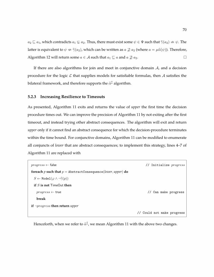
70
a2 v a1, which contradicts a1 Ĺ a2. Thus, there must exist some ψ ∈ Ψ such that γ(a2) ; ψ. The
latter is equivalent to ψ : γ(a2), which can be written as a 6w a2 (where a = µα(ψ)). Therefore,
Algorithm 12 will return some a ∈ A such that a1 v a and a 6w a2.
If there are also algorithms for join and meet in conjunctive domain A, and a decision
procedure for the logic L that supplies models for satisfiable formulas, then A satisfies the
bilateral framework, and therefore supports the αl algorithm.
5.2.3 Increasing Resilience to Timeouts
As presented, Algorithm 11 exits and returns the value of upper the first time the decision
procedure times out. We can improve the precision of Algorithm 11 by not exiting after the first
timeout, and instead trying other abstract consequences. The algorithm will exit and return
upper only if it cannot find an abstract consequence for which the decision-procedure terminates
within the time bound. For conjunctive domains, Algorithm 11 can be modified to enumerate
all conjuncts of lower that are abstract consequences; to implement this strategy, lines 4–7 of
Algorithm 11 are replaced with
progress← false // Initialize progress
foreach p such that p = AbstractConsequence(lower,upper) do
S ← Model(ϕ ∧ ¬γ(p))
if S is not TimeOut then
progress← true // Can make progress
break
if ¬progress then return upper
// Could not make progress
Henceforth, when we refer to αl, we mean Algorithm 11 with the above two changes.

71
5.2.4 Relationship of Abstract Consequence to Interpolation
To avoid the potential for confusion, we now discuss how the notion of abstract consequence
differs from the well-known concept of interpolation (Craig, 1957):
A logic L supports interpolation if for all ϕ1, ϕ2 ∈ L such that ϕ1⇒ϕ2, there exists a
formula I such that (i) ϕ1⇒ I , (ii) I⇒ϕ2, and (iii) I uses only symbols in the shared
vocabulary of ϕ1 and ϕ2.
Although condition (i) is part of Definition 5.1, the restrictions imposed by conditions (ii) and
(iii) are not part of Definition 5.1. To highlight the differences, we restate Definition 5.1 in terms
of formulas.
An operation AbstractConsequence(·, ·) is an acceptable abstract-consequence oper-
ation iff for all a1, a2 ∈ A such that γ(a1)⇒ γ(a2) and γ(a1) : γ(a2),
a = AbstractConsequence(a1, a2) implies γ(a1)⇒ γ(a) and γ(a) : γ(a2).
From an operational standpoint, condition (iii) in the definition of interpolation serves as a
heuristic that generally allows interpolants to be expressed as small formulas. In the context of
αl, we are interested in obtaining small formulas to use in the decision-procedure query (line 5
of Algorithm 11). Thus, given a1, a2 ∈ A, it might appear plausible to use an interpolant I of
γ(a1) and γ(a2) in αl instead of the abstract consequence of a1 and a2. However, there are a few
problems with such an approach:
• There is no guarantee that I will indeed be simple; for instance, if the vocabulary of γ(a1) is
a subset of the vocabulary of γ(a2), then I could be γ(a1) itself, in which case Algorithm 11
performs the more expensive RSY iteration step.
• Converting the formula I into an abstract value p ∈ A for use in line 9 of Algorithm 11
itself requires performing α on I .

72
Algorithm 13: αl+〈L,A〉(ϕ)1 upper← >2 lower← ⊥3 k ← 0 // initialize k4 while lower 6= upper do
// lower Ĺ upper5 if k < N then6 p← AbstractConsequence(lower,upper)7 else8 p← lower// p w lower, p 6w upper9 S ← Model(ϕ ∧ ¬γ(p))
10 if S is TimeOut then11 return upper12 else if S is None then // ϕ⇒ γ(p)13 upper← upper u p14 k ← k + 1 // increment k
15 else // S 6|= γ(p)16 lower← lower t β(S)17 k ← 0 // reset k
18 ans← upper19 return ans
As discussed above, many domains are conjunctive domains, and for conjunctive domains is
it always possible to find a single conjunct that is an abstract consequence (see Theorem 5.3).
Moreover, such a conjunct is not necessarily an interpolant.
5.3 Abstract Domains with Infinite Descending Chains
We can weaken part 2 of Theorem 5.2 to allowA to have infinite descending chains by modifying
Algorithm 11 slightly. The modified algorithm has to ensure that it does not get trapped updating
upper along an infinite descending chain, and that it exits when lower has converged to α(ϕ).
Suppose that, for some fixed N , N consecutive iterations of the loop on lines 3–11 update upper
(line 9) without updating lower (line 11). If this situation occurs, in the next iteration the algorithm
can set p to lower so that the decision-procedure query at line 5 becomes Model(ϕ ∧ ¬γ(lower))—
i.e., we force the algorithm to perform the basic iteration-step from the RSY algorithm. In this

73
way, we force lower to be updated at least once every N iterations. Moreover, if on such an
RSY-step the model S returned from the decision procedure is None, then we know that lower
has converged to α(ϕ) and the algorithm can return. A version of Algorithm 11 that implements
this strategy is presented as Algorithm 13.
Theorem 5.4. If abstract domain A does not have infinite ascending chains, and Algorithm 13 does not
timeout, then αl+〈L,A〉(ϕ) terminates and returns α(ϕ).
Proof. The proof of Theorem 5.2 carries over, except that we must additionally argue that if A
has infinite descending chains, αl+ (Algorithm 13) does not get trapped refining upper along an
infinite descending chain, and that the algorithm returns α(ϕ) after lower has converged to α(ϕ).
Suppose that N consecutive iterations of the loop on lines 3–11 update upper (line 13) without
updating lower (line 16). In the next iteration, the algorithm can set p to lower (line 8 so that the
decision-procedure query at line 9 becomes Model(ϕ ∧ ¬γ(lower))—i.e., we force the algorithm
to perform the basic iteration-step from the RSY algorithm. In this way, we force lower to be
updated at least once every N iterations.
Consequently, becauseA has no infinite ascending chains, lower must eventually be set to α(ϕ).
After that happens, within the next N iterations of the loop body, Algorithm 13 must execute
line 8, which sets p to lower (i.e., p = α(ϕ)). The model S returned from calling Model(ϕ∧¬γ(p))
in line 9 must be None. As argued in the proof of Theorem 5.2, lower v α(ϕ) v upper holds
on every iteration of the loop in lines 4–17. Because α(ϕ) v upper and p = α(ϕ), the update
upper ← upper u p on line 13 assigns α(ϕ) to upper. Because lower is equal to upper, the loop
exits with upper = α(ϕ). At line 18, ans is thus assigned α(ϕ), which is the value returned by
Algorithm 13 at line 19.
5.3.1 Algorithm Complexity
In this section, I analyze the worst-case time complexity of Algorithm 13. I first state the time
complexity of the algorithm for a generic abstract domain A and logic L. I then talk about the
time complexity for the affine-equalities abstract domain E2w and QFBV logic.

74
The worst-case time complexity T of Algorithm 13 for abstract domain A and logic L is
T = O(C × (TAC + TDP + TAO)) (5.3)

75
where
• C is the maximum length of an ascending chain in A, which is an upper bound for the
number of times the loop in lines 4–17 executes,
• TAC is the time complexity of computing the abstract consequence on line 6,
• TDP is the time complexity of the call to the decision procedure for logic L on line 9,
• TAO is the time complexity of the abstract operations, meet, on line 13, and join, on line 16).
Consider the instantiation of Algorithm 13 with the affine-equalities abstract domain E2w
and QFBV logic. Let k be the number of variables that the abstract domain E2w keeps track of. I
now list the various parameters in Equation (5.3) for this specific instantiation of the bilateral
algorithm:
• The length of the longest ascending chain in E2w is O(wk) (Elder et al., 2014, Theorem 2.7).
• The abstract consequence is computed using Algorithm 12. The loop on lines 4–6 can
execute at most k times. The time complexity of the subsumption check on line 6 is
O(k3) (Elder et al., 2014).Thus, the worst-case time complexity for computing the abstract
consequence is TAC = O(k4).
• The decision procedure for QFBV logic is NEXPTIME-complete (Kovásznai et al., 2012).
• The worst-case time complexity of the meet and join operations for E2w are O(k3) (Elder
et al., 2014).
Note that, technically, the time complexity of subsumption, meet, and join for E2w depends
on an operation that has the same asymptotic complexity as matrix multiplication (Storjohann,
2000). The operation has a straightforward O(k3) implementation that is similar to a standard
Gaussian-elimination algorithm (Elder et al., 2014, Algorithm 1).

76
5.4 Instantiations
In this section, we describe instantiations of the bilateral framework for several abstract domains.
5.4.1 Herbrand-Equalities Domain
Herbrand equalities are used in analyses for partial redundancy elimination, loop-invariant
code motion (Steffen et al., 1990), and strength reduction (Steffen et al., 1991). In these analyses,
arithmetic operations (e.g., + and *) are treated as term constructors. Two program variables
are known to hold equal values if the analyzer determines that the variables hold equal terms.
Herbrand equalities can also be used to analyze programs whose types are user-defined algebraic
data-types.
Basic definitions. Let F be a set of function symbols. The function arity : F → N yields the
number of parameters of each function symbol. Terms over F are defined in the usual way; each
function symbol f ∈ F always requires arity(f) parameters. Let T (F , X) denote the set of finite
terms generated by F and variable set X . The Herbrand universe of F is T (F , ∅), the set of ground
terms over F .
A Herbrand state is a mapping from program variables V to ground terms (i.e., a function in
V → T (F , ∅)). The concrete domain consists of all sets of Herbrand states: C def= P (V → T (F , ∅)).
We can apply a Herbrand state σ to a term t ∈ T (F ,V) as follows:
σ[t] def=
σ(t) if t ∈ V
f(σ[t1], . . . , σ[tk]) if t = f(t1, . . . , tk)
The Herbrand-equalities domain. Sets of Herbrand states can be abstracted in several ways. One
way is to use conjunctions of equations among terms (whence the name “Herbrand-equalities
domain”). Such systems of equations can be represented using Equivalence DAGs (Steffen
et al., 1990). A different, but equivalent, approach is to use a representation based on idempotent
substitutions: A = (V → T (F ,V))⊥. Idempotence means that for each σ 6= ⊥ and v ∈ V ,
σ[σ(v)] = σ(v). The meaning of an idempotent substitution σ ∈ A is given by its concretization

77
γ(σ), where γ : A → C, γ(⊥) = ∅, and otherwise
γ(σ) = {ρ : V → T (F , ∅) | ∀v ∈ V : ρ(v) = ρ[σ(v)]} . (5.4)
I now show that the Herbrand-equalities domain satisfies the requirements of the bilateral
framework. I will assume that the logical language L has all the function symbols and constant
symbols from F , equality, and a constant symbol for each element from V1. (In a minor abuse of
notation, the set of such constant symbols will also be denoted by V .) The logic’s universe is the
Herbrand universe of F (i.e., T (F , ∅)). An interpretation maps the constants in V to terms in
T (F , ∅). To be able to express γ(p) and ¬γ(p) (see item 3 below), we assume that L contains at
least the following productions:
F ::= F ∧ F | ¬F | v = T for v ∈ V | false
T ::= v ∈ V | f(T1, . . . , Tk) when arity(f) = k(5.5)
1. There is a Galois connection C −−→←−−αγA:
• The ordering on C is the subset relation on sets of Herbrand states.
• γ(σ) is given in Equation (5.4).
• α(S) = {a | γ(a) ⊇ S}.
• For a, b ∈ A, a v b iff γ(a) ⊆ γ(b).
2. Meet is most-general unification of substitutions, computed by standard unification tech-
niques (Lassez et al., 1988, Thm. 3.1). Join is most-specific generalization, computed by
“dual unification” or “anti-unification” (Plotkin, 1970; Reynolds, 1970), (Lassez et al., 1988,
Thm. 5.8). Equality checking is described by Lassez et al. (Lassez et al., 1988, Prop. 4.10).
3. γ: γ(⊥) = false; otherwise, γ(σ) is∧v∈V v = σ(v).
1Because the set of program variables is finite, V is finite.

78
4. A decision procedure for L, with models, is given by Lassez et al. (Lassez et al., 1988,
Thm. 6.12). In practice, one can obtain a decision procedure for L formulas using the
built-in datatype mechanism of, e.g., Z3 (de Moura and Bjørner, 2008) or Yices (Dutertre
and de Moura, 2006), and obtain the necessary decision procedure using an existing SMT
solver.
5. L is closed under conjunction and negation.
6. AbstractConsequence: The domain is a conjunctive domain, as can be seen from the
definition of γ.
Theorem 5.2 ensures that Algorithm 11 returns α(ϕ) when abstract domain A has neither
infinite ascending nor infinite descending chains. The Herbrand-equalities domain has no infinite
ascending chains (Lassez et al., 1988, Lem. 3.15). The domain described here also has no infinite
descending chains, essentially because every right-hand term in every Herbrand state has no
variables but those in V .2
I now present a pair of worked examples of αl (Algorithm 11) for the Herbrand-equalities
domain.
Example 5.5. Consider the following code fragment, which uses two different methods forchecking the parity of i (i&1 and i << 31 == 0):
i n t i ;cons_ t ree x , y ;x = ( i &1) ? n i l : cons ( y , x ) ;i f ( i << 31 == 0 ) { /∗ ( ∗ ) . . . ∗ / }
Suppose that we want an element of the Herbrand-equalities domain that relates the values of
x and y at the fragment’s start to x′ and y′, the values of those variables at program point (*).
A straightforward abstract interpretation of this program in the Herbrand-equalities domain
would yield no information about x′, because {x′ 7→ nil}t {x′ 7→ cons(y, x)} = {x′ 7→ x′}.2One can instead define a domain of Herbrand equalities in which fresh variables may occur in the terms of
an idempotent substitution’s range. Everything said in this section remains true of this alternative domain, exceptthat it has infinite descending chains, and so Algorithm 11 is only guaranteed to return an over-approximation ofα(ϕ). However, as discussed in Section 5.2, Algorithm 13, presented in Section 5.3, is a version of Algorithm 11 thatconverges to α(ϕ), even when the abstract domain has infinite descending chains.
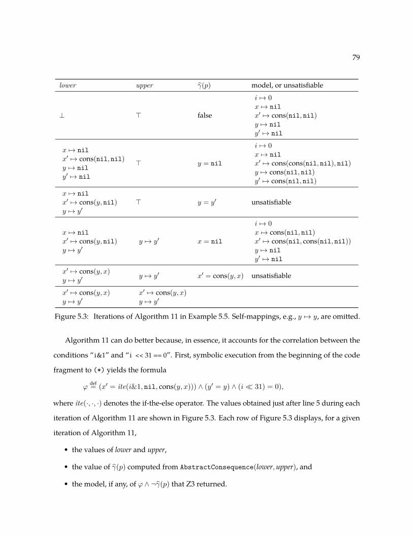
79
lower upper γ(p) model, or unsatisfiable
⊥ > false
i 7→ 0x 7→ nilx′ 7→ cons(nil, nil)y 7→ nily′ 7→ nil
x 7→ nilx′ 7→ cons(nil, nil)y 7→ nily′ 7→ nil
> y = nil
i 7→ 0x 7→ nilx′ 7→ cons(cons(nil, nil), nil)y 7→ cons(nil, nil)y′ 7→ cons(nil, nil)
x 7→ nilx′ 7→ cons(y, nil)y 7→ y′
> y = y′ unsatisfiable
x 7→ nilx′ 7→ cons(y, nil)y 7→ y′
y 7→ y′ x = nil
i 7→ 0x 7→ cons(nil, nil)x′ 7→ cons(nil, cons(nil, nil))y 7→ nily′ 7→ nil
x′ 7→ cons(y, x)y 7→ y′
y 7→ y′ x′ = cons(y, x) unsatisfiable
x′ 7→ cons(y, x)y 7→ y′
x′ 7→ cons(y, x)y 7→ y′
Figure 5.3: Iterations of Algorithm 11 in Example 5.5. Self-mappings, e.g., y 7→ y, are omitted.
Algorithm 11 can do better because, in essence, it accounts for the correlation between the
conditions “i&1” and “i << 31 == 0”. First, symbolic execution from the beginning of the code
fragment to (*) yields the formula
ϕdef= (x′ = ite(i&1, nil, cons(y, x))) ∧ (y′ = y) ∧ (i� 31) = 0),
where ite(·, ·, ·) denotes the if-the-else operator. The values obtained just after line 5 during each
iteration of Algorithm 11 are shown in Figure 5.3. Each row of Figure 5.3 displays, for a given
iteration of Algorithm 11,
• the values of lower and upper,
• the value of γ(p) computed from AbstractConsequence(lower,upper), and
• the model, if any, of ϕ ∧ ¬γ(p) that Z3 returned.
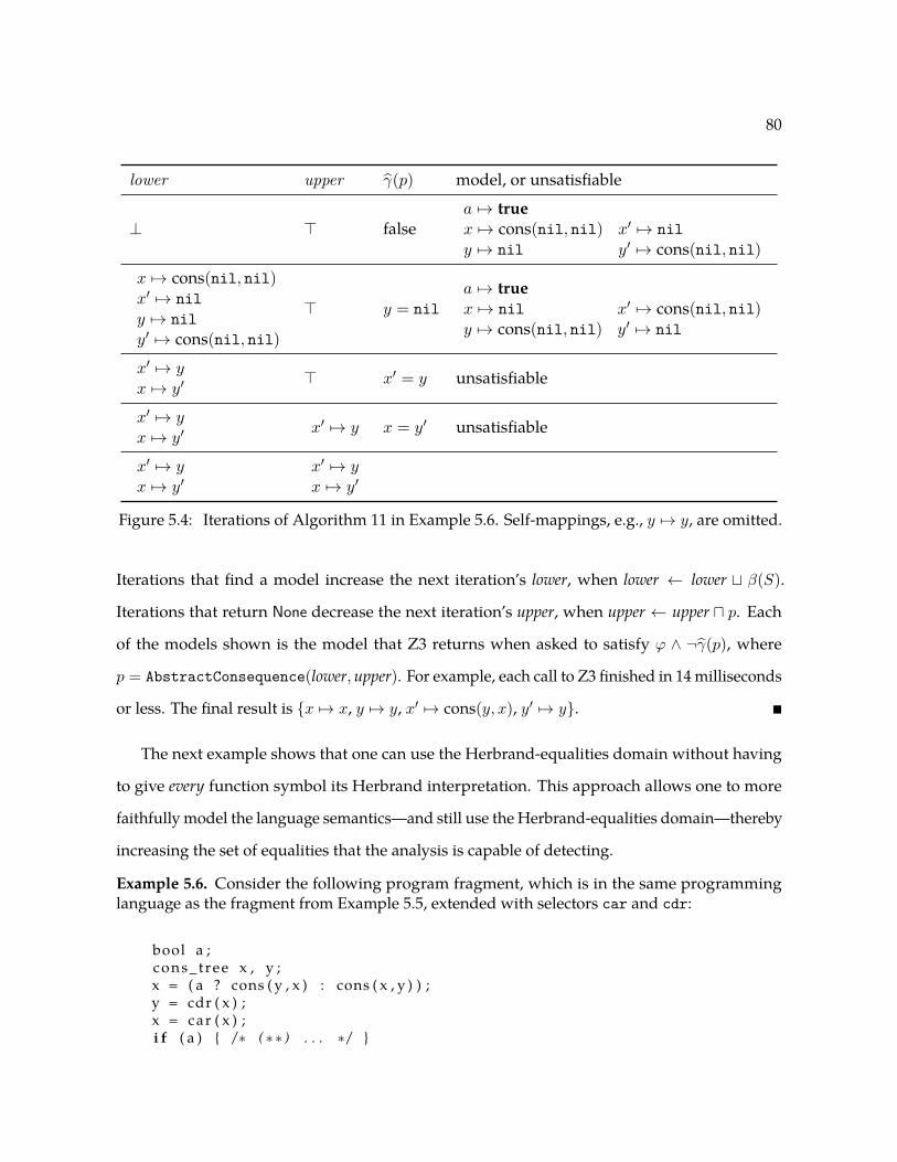
80
lower upper γ(p) model, or unsatisfiable
⊥ > falsea 7→ truex 7→ cons(nil, nil) x′ 7→ nily 7→ nil y′ 7→ cons(nil, nil)
x 7→ cons(nil, nil)x′ 7→ nily 7→ nily′ 7→ cons(nil, nil)
> y = nila 7→ truex 7→ nil x′ 7→ cons(nil, nil)y 7→ cons(nil, nil) y′ 7→ nil
x′ 7→ yx 7→ y′
> x′ = y unsatisfiable
x′ 7→ yx 7→ y′
x′ 7→ y x = y′ unsatisfiable
x′ 7→ yx 7→ y′
x′ 7→ yx 7→ y′
Figure 5.4: Iterations of Algorithm 11 in Example 5.6. Self-mappings, e.g., y 7→ y, are omitted.
Iterations that find a model increase the next iteration’s lower, when lower ← lower t β(S).
Iterations that return None decrease the next iteration’s upper, when upper ← upper u p. Each
of the models shown is the model that Z3 returns when asked to satisfy ϕ ∧ ¬γ(p), where
p = AbstractConsequence(lower,upper). For example, each call to Z3 finished in 14 milliseconds
or less. The final result is {x 7→ x, y 7→ y, x′ 7→ cons(y, x), y′ 7→ y}. �
The next example shows that one can use the Herbrand-equalities domain without having
to give every function symbol its Herbrand interpretation. This approach allows one to more
faithfully model the language semantics—and still use the Herbrand-equalities domain—thereby
increasing the set of equalities that the analysis is capable of detecting.
Example 5.6. Consider the following program fragment, which is in the same programminglanguage as the fragment from Example 5.5, extended with selectors car and cdr:
bool a ;cons_ t ree x , y ;x = ( a ? cons ( y , x ) : cons ( x , y ) ) ;y = cdr ( x ) ;x = car ( x ) ;i f ( a ) { /∗ (∗∗ ) . . . ∗ / }
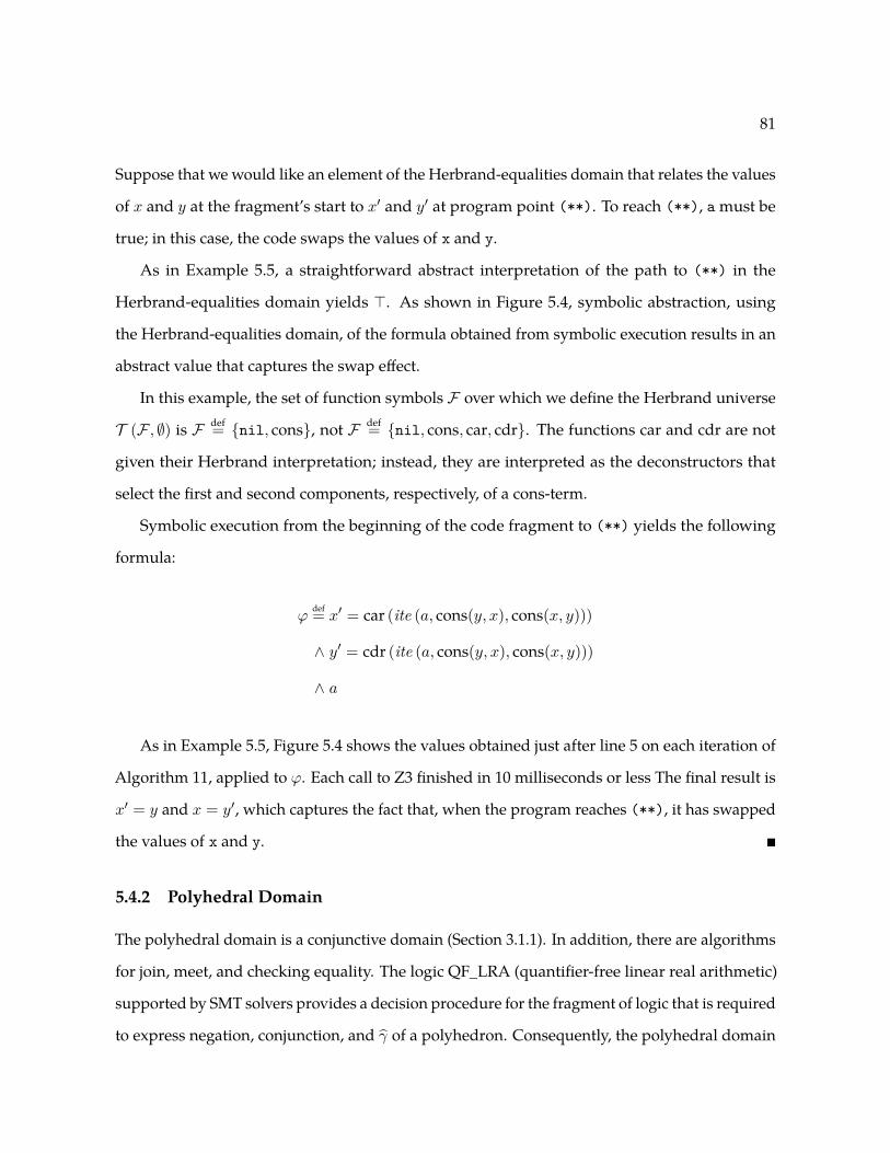
81
Suppose that we would like an element of the Herbrand-equalities domain that relates the values
of x and y at the fragment’s start to x′ and y′ at program point (**). To reach (**), a must be
true; in this case, the code swaps the values of x and y.
As in Example 5.5, a straightforward abstract interpretation of the path to (**) in the
Herbrand-equalities domain yields >. As shown in Figure 5.4, symbolic abstraction, using
the Herbrand-equalities domain, of the formula obtained from symbolic execution results in an
abstract value that captures the swap effect.
In this example, the set of function symbols F over which we define the Herbrand universe
T (F , ∅) is F def= {nil, cons}, not F def= {nil, cons, car, cdr}. The functions car and cdr are not
given their Herbrand interpretation; instead, they are interpreted as the deconstructors that
select the first and second components, respectively, of a cons-term.
Symbolic execution from the beginning of the code fragment to (**) yields the following
formula:
ϕdef= x′ = car (ite (a, cons(y, x), cons(x, y)))
∧ y′ = cdr (ite (a, cons(y, x), cons(x, y)))
∧ a
As in Example 5.5, Figure 5.4 shows the values obtained just after line 5 on each iteration of
Algorithm 11, applied to ϕ. Each call to Z3 finished in 10 milliseconds or less The final result is
x′ = y and x = y′, which captures the fact that, when the program reaches (**), it has swapped
the values of x and y. �
5.4.2 Polyhedral Domain
The polyhedral domain is a conjunctive domain (Section 3.1.1). In addition, there are algorithms
for join, meet, and checking equality. The logic QF_LRA (quantifier-free linear real arithmetic)
supported by SMT solvers provides a decision procedure for the fragment of logic that is required
to express negation, conjunction, and γ of a polyhedron. Consequently, the polyhedral domain
82
upperlower
(a) (b) (c)
p
Figure 5.5: Abstract consequence on polyhedra. (a) Two polyhedra: lower v upper. (b) p =AbstractConsequence(lower,upper). (c) Result of upper← upper u p.
satisfies the bilateral framework, and therefore supports the αl algorithm. The polyhedral domain
has both infinite ascending chains and infinite descending chains, and hence Algorithm 13 is
only guaranteed to compute an over-approximation of α(ϕ).
Because the polyhedral domain is a conjunctive domain, if lower Ĺ upper, then some single
constraint p of lower satisfies p 6w upper. For instance, if lower and upper are the polyhedra shown
in Figure 5.5(a), then the region p above the dotted line in Figure 5.5(b) is an acceptable abstract
consequence. Figure 5.5(c) shows the result after upper ← upper u p is performed at line 9 of
Algorithm 11.
5.5 Empirical Comparison of the KS and Bilateral Algorithms
In this section, I compare two algorithms for performing symbolic abstraction for the affine-
equalities domain E232 :
• the α↑KS procedure of Algorithm 7.
• the αl〈E232〉 procedure that is the instantiation of Algorithm 11 for the domain of affine-
equalities E232 and QFBV logic.
Although the bilateral algorithm αl〈E232〉 benefits from being resilient to timeouts, it maintains
both an over-approximation and an under-approximation. Thus, the experiments were designed
to understand the trade-off between performance and precision.
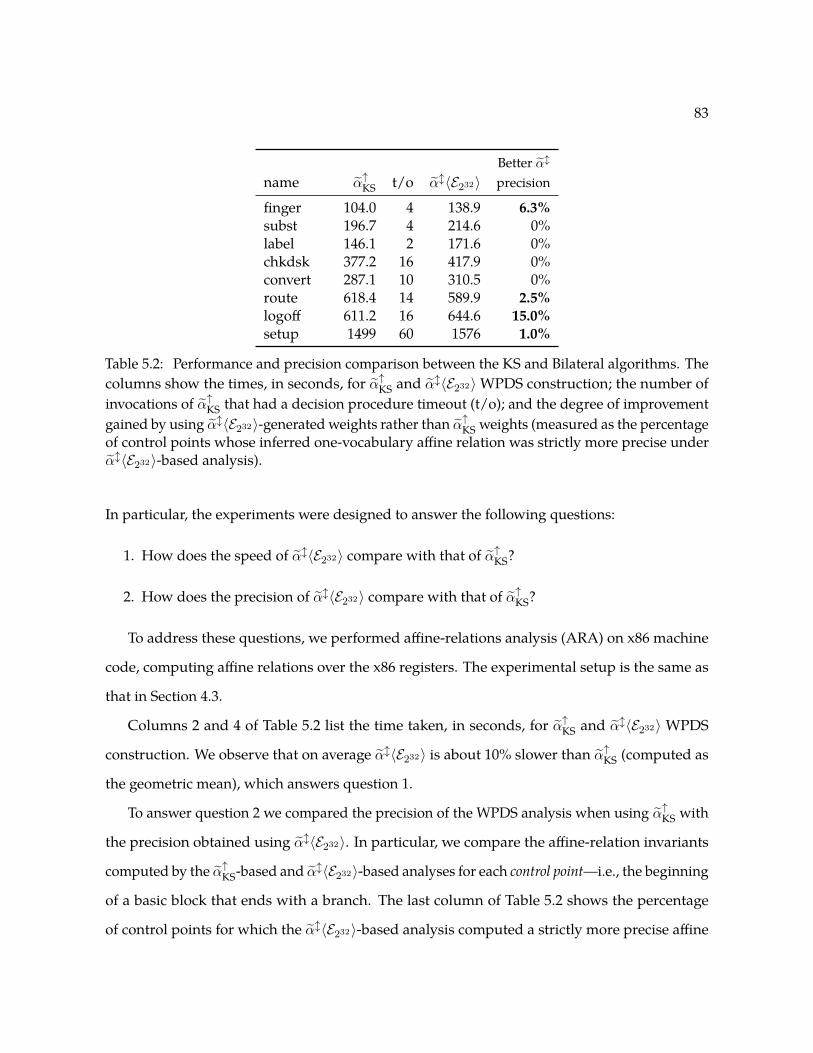
83
Better αl
name α↑KS t/o αl〈E232〉 precision
finger 104.0 4 138.9 6.3%subst 196.7 4 214.6 0%label 146.1 2 171.6 0%chkdsk 377.2 16 417.9 0%convert 287.1 10 310.5 0%route 618.4 14 589.9 2.5%logoff 611.2 16 644.6 15.0%setup 1499 60 1576 1.0%
Table 5.2: Performance and precision comparison between the KS and Bilateral algorithms. Thecolumns show the times, in seconds, for α↑KS and αl〈E232〉WPDS construction; the number ofinvocations of α↑KS that had a decision procedure timeout (t/o); and the degree of improvementgained by using αl〈E232〉-generated weights rather than α↑KS weights (measured as the percentageof control points whose inferred one-vocabulary affine relation was strictly more precise underαl〈E232〉-based analysis).
In particular, the experiments were designed to answer the following questions:
1. How does the speed of αl〈E232〉 compare with that of α↑KS?
2. How does the precision of αl〈E232〉 compare with that of α↑KS?
To address these questions, we performed affine-relations analysis (ARA) on x86 machine
code, computing affine relations over the x86 registers. The experimental setup is the same as
that in Section 4.3.
Columns 2 and 4 of Table 5.2 list the time taken, in seconds, for α↑KS and αl〈E232〉WPDS
construction. We observe that on average αl〈E232〉 is about 10% slower than α↑KS (computed as
the geometric mean), which answers question 1.
To answer question 2 we compared the precision of the WPDS analysis when using α↑KS with
the precision obtained using αl〈E232〉. In particular, we compare the affine-relation invariants
computed by the α↑KS-based and αl〈E232〉-based analyses for each control point—i.e., the beginning
of a basic block that ends with a branch. The last column of Table 5.2 shows the percentage
of control points for which the αl〈E232〉-based analysis computed a strictly more precise affine

84
Algorithm 14: Post↑[τ ](v)
1
2 lower′ ← ⊥3 while true do4
5 〈S, S′〉 ← Model(γ(v) ∧ τ ∧ ¬γ( lower′ ))6 if 〈S, S′〉 is TimeOut then7 return >8 else if 〈S, S′〉 is None then9 break // Post[τ ](v)= lower′
10 else // S′ 6|= γ(lower′ )11 lower′ ← lower′ t β(S′)12 v′ ← lower′
13 return v’
Algorithm 15: Postl[τ ](v)
1 upper′ ← >2 lower′ ← ⊥3 while lower′ 6= upper′ ∧ ResourcesLeft do4 p′ ← AbstractConsequence(lower′,upper′)// p′ w lower′, p′ 6w upper′
5 〈S, S′〉 ← Model(γ(v) ∧ τ ∧ ¬γ(p′ ))6 if 〈S, S′〉 is TimeOut then7 break8 else if 〈S, S′〉 is None then9 upper′ ← upper′ u p′ // Post[τ ](v)v p′
10 else // S′ 6|= γ(p′ )11 lower′ ← lower′ t β(S′)12 v′ ← upper′
13 return v’
relation. Column 3 of Table 5.2 lists the number invocations of α↑KS that had a decision-procedure
timeout, and hence returned >. We see that the αl〈E232〉-based analysis improves precision at
up to 15% of control points, and, on average, the αl〈E232〉-based analysis is more precise for 3.1%
of the control points (computed as the arithmetic mean), which answers question 2.
5.6 Computing Post
Algorithm 15 shows the Bilateral algorithm for computing Post. In the same way Algorithm 6,
which computes symbolic abstraction, was adapted to give Algorithm 8, which computes Post,
Algorithm 11 is adapted to give Algorithm 15. The differences between Post↑
and Postl
are
highlighted in gray. Most concern the variables upper′ or p′. Algorithm 8 will be used in Chapter 7.
5.7 Related Work
5.7.1 Related Work on Symbolic Abstraction
Previous work on symbolic abstraction falls into three categories:
1. algorithms for specific domains (Regehr and Reid, 2004; McMillan, 2005; Brauer and King,
2010; Barrett and King, 2010; King and Søndergaard, 2010; Elder et al., 2011; Li et al., 2014)

85
2. algorithms for parameterized abstract domains (Graf and Saïdi, 1997; Yorsh et al., 2004;
Sankaranarayanan et al., 2005; Monniaux, 2010)
3. abstract-domain frameworks (Reps et al., 2004).
What distinguishes category 3 from category 2 is that each of the results cited in category 2
applies to a specific family of abstract domains, defined by a parameterized Galois connection (e.g.,
with an abstraction function equipped with a readily identifiable parameter for controlling the
abstraction). In contrast, the results in category 3 are defined by an interface; for any abstract
domain that satisfies the requirements of the interface, one has a method for symbolic abstraction.
The approach presented in this paper falls into category 3.
Algorithms for specific domains. Regehr and Reid (2004) present a method that constructs
abstract transformers for machine instructions, for interval and bitwise abstract domains. Their
method does not call a SAT solver, but instead uses the physical processor (or a simulator of a
processor) as a black box. To compute the abstract post-state for an abstract value a, the approach
recursively divides a until an abstract value is obtained whose concretization is a singleton set.
The concrete semantics are then used to derive the post-state value. The results of each division
are joined as the recursion unwinds to derive the abstract post-state value.
Brauer and King (2010) developed a method that works from below to derive abstract trans-
formers for the interval domain. Their method is based on an approach due to Monniaux (2010)
(see below), but they changed two aspects:
1. They express the concrete semantics with a Boolean formula (via “bit-blasting”), which
allows a formula equivalent to ∀x.ϕ to be obtained from ϕ (in CNF) by removing the x and
¬x literals from all of the clauses of ϕ.
2. Whereas Monniaux’s method performs abstraction and then quantifier elimination, Brauer
and King’s method performs quantifier elimination on the concrete specification, and then
performs abstraction.

86
The abstract transformer derived from the Boolean formula that results is a guarded update:
the guard is expressed as an element of the octagon domain (Miné, 2001); the update operation
is expressed as an element of the abstract domain of rational affine equalities (Karr, 1976).
The abstractions performed to create the guard and the update are optimal for their respective
domains. The algorithm they use to create the abstract value for the update operation is essentially
the King-Søndergaard algorithm for α (King and Søndergaard, 2010, Fig. 2), which works from
below (see Algorithm 7). Brauer and King show that optimal evaluation of such transfer functions
requires linear programming. They give an example that demonstrates that an octagon-closure
operation on a combination of the guard’s octagon and the update’s affine equality is sub-optimal.
Barrett and King (2010) describe a method for generating range and set abstractions for bit-
vectors that are constrained by Boolean formulas. For range analysis, the algorithm separately
computes the minimum and maximum value of the range for an n-bit bit-vector using 2n calls to
a SAT solver, with each SAT query determining a single bit of the output. The result is the best
over-approximation of the value that an integer variable can take on (i.e., α).
Li et al. (2014) developed a symbolic-abstraction method for LRA, called SYMBA. The scenario
considered by Li et al. (2014) differs from that considered in this thesis. Given a formula ϕ in LRA
logic and a finite set of objectives {t1, t2, . . . , tn}, where ti is a linear-rational expression, SYMBA
computes the lower and upper bounds l1, l2, . . . , ln and u1, u2, . . . , un such that ϕ⇒(∧
1≤i≤n li ≤
ti ≤ ui). Similar to the Bilateral framework described in this chapter, the SYMBA algorithm
maintains and under-approximation and over-approximation of the final answer.
McMillan (2005) presents an algorithm for performing symbolic abstraction for propositional
logic and the abstract domain of propositional clauses of length up to k. The algorithm can be
viewed as an instance of the RSY algorithm: a SAT solver is used to generate samples and a trie
data structure is used to perform the join of abstract values. The specific application that the
algorithm is used for is to compute don’t-care conditions for logic synthesis.
Algorithms for parameterized abstract domains. Graf and Saïdi (1997) showed that decision
procedures can be used to generate best abstract transformers for predicate-abstraction domains.
Other work has investigated more efficient methods to generate approximate transformers that
87
are not best transformers, but approach the precision of best transformers (Ball et al., 2001; Clarke
et al., 2004).
Yorsh et al. (2004) developed a method that works from above to perform α(ϕ) for the kind of
abstract domains used in shape analysis (i.e., “canonical abstraction” of logical structures (Sagiv
et al., 2002)).
Template Constraint Matrices (TCMs) are a parametrized family of linear-inequality domains
for expressing invariants in linear real arithmetic. Sankaranarayanan et al. (2005) gave a meet,
join, and set of abstract transformers for all TCM domains. Monniaux (2010) gave an algorithm
that finds the best transformer in a TCM domain across a straight-line block (assuming that
concrete operations consist of piecewise linear functions), and good transformers across more
complicated control flow. However, the algorithm uses quantifier elimination, and no polynomial-
time elimination algorithm is known for piecewise-linear systems.
Abstract-domain frameworks. As discussed in Section 5.2, the bilateral framework reduces to
the RSY framework when using a particular (trivial) implementation of AbstractConsequence.
Unlike the RSY framework, to compute α(ϕ) the bilateral framework does not impose the re-
quirement that the abstract domain have no infinite ascending chains. As shown in part 1 of
Theorem 5.2, even when there are infinite ascending chains, the bilateral framework can return a
non-trivial over-approximation of α(ϕ). In contrast, RSY gives no such guarantees. Consequently,
compared to the RSY framework, the bilateral framework is applicable to a larger class of abstract
domains.
5.7.2 Other Related Work
Logical abstract domains. Cousot et al. (2011a) define a method of abstract interpretation based
on using particular sets of logical formulas as abstract-domain elements (so-called logical abstract
domains). They face the problems of (i) performing abstraction from unrestricted formulas to
the elements of a logical abstract domain (Cousot et al., 2011a, §7.1), and (ii) creating abstract
transformers that transform input elements of a logical abstract domain to output elements of

88
the domain (Cousot et al., 2011a, §7.2). Their problems are particular cases of α(ϕ). They present
heuristic methods for creating over-approximations of α(ϕ).
Connections to machine-learning algorithms.
α↑RSY (Algorithm 6) is related to the Find-S algorithm (Mitchell, 1997, Section 2.4) for concept
learning. Both algorithms start with the most-specific hypothesis (i.e., ⊥) and work bottom-up
to find the most-specific hypothesis that is consistent with positive examples of the concept.
Both algorithms generalize their current hypothesis each time they process a (positive) training
example that is not explained by the current hypothesis. A major difference is that Find-S receives
a sequence of positive and negative examples of the concept (e.g., from nature). It discards
negative examples, and its generalization steps are based solely on the positive examples. In
contrast, α↑RSY already starts with a precise statement of the concept in hand, namely, the formula
ϕ, and on each iteration, calls a decision procedure to generate the next positive example; α↑RSY
never sees a negative example.
A similar connection exists between αl (Algorithm 11) and the Candidate-Elimination (CE)
algorithm for concept learning (Mitchell, 1997, Section 2.5). Both algorithms maintain two
approximations of the concept, one that is an over-approximation and one that is an under-
approximation. The CE algorithm updates its under-approximation using positive examples in
the same way that the Find-S algorithm updates its under-approximation. Similarly, the Bilateral
algorithm updates its under-approximation (via a join) is the same way that the RSY algorithm
updates its under-approximation. One key difference between the CE algorithm and the Bilateral
algorithm is that the CE algorithm updates its over-approximation using negative examples. Most
conjunctive abstract domains are not closed under negation. Thus, given a negative example,
there usually does not exist an abstract value that only excludes that particular negative example.
5.8 Chapter Notes
The idea for the KS+ algorithm occurred to me during Andy King’s talk at a Dagstuhl seminar
describing the results of (King and Søndergaard, 2010). Though I was familiar with the paper,

89
I had never internalized the working of KS algorithm properly. The generalization of the KS+
algorithm to the Bilateral framework followed naturally from the requirement that each iteration
of the Bilateral algorithm is required to make progress.
The concept of Abstract Consequence was concealed inside the KS algorithm, and had to
be gleaned out. The concept of abstract consequence was used implicitly, and an acceptable
abstract consequence was computed by reading a single row of a matrix in Howell form (line 5
of Algorithm 9).
The main surprise was that the Howell form, a normal form using for the E2w abstract domain,
stressed in Elder et al. (2011) was not of central importance in generalizing the KS algorithm;
instead the Abstract Consequence operation was the key.

90
Chapter 6
A Generalization of Stålmarck’s
Method
In building a statue, a sculptor doesn’t keep adding clay to his
subject. Actually, he keeps chiselling away at the inessentials
until the truth of its creation is revealed without obstructions.— Bruce Lee
As explained in Section 3.4, Stålmarck’s method (Sheeran and Stålmarck, 2000) is an algo-
rithm for checking satisfiability of a formula in propositional logic. In this chapter, I give a new
account of Stålmarck’s method by explaining each of the key components in terms of concepts
from the field of abstract interpretation. In particular, I show that Stålmarck’s method can be
viewed as a general framework, which I call Stålmarck[A], that is parameterized on an abstract
domain A and operations on A. This abstraction-based view allows Stålmarck’s method to
be lifted from propositional logic to richer logics, such as LRA. Furthermore, the generalized
Stålmarck’s method falls into the Satisfiability Modulo Abstraction (SMA) paradigm: the gener-
alized Stålmarck’s-method solver we created is designed and implemented using concepts from
abstract interpretation.
91
In this chapter, I use the vantage point of abstract interpretation to describe the elements of
the Dilemma Rule as follows:
Branch of a Proof: In Stålmarck’s method, each proof-tree branch is associated with a so-called
formula relation (Sheeran and Stålmarck, 2000). In abstract-interpretation terms, each branch
is associated with an abstract-domain element.
Splitting: The step of splitting the current goal into sub-goals can be expressed in terms of
meet (u).
Application of simple deductive rules: Stålmarck’s method applies a set of simple deductive
rules after each split. In abstract-interpretation terms, the rules perform a semantic reduction
(Cousot and Cousot, 1979).
“Intersecting” results: The step of combining the results obtained from an earlier split are
described as an “intersection” in Stålmarck’s papers. In the abstract-interpretation-based
framework, the combining step is the join (t) of two abstract-domain values.
This more general view of Stålmarck’s method furnishes insight on when an invocation of the
Dilemma Rule fails to make progress in a proof. In particular, both branches of a Dilemma may
each succeed (locally) in advancing the proof, but the abstract domain used to represent proof
states may not be precise enough to represent the common information when the join of the two
branches is performed; consequently, the global state of the proof is not advanced.
As mentioned in Section 1.2, the other advantage of the abstraction-based view of Stålmarck’s
method is that it brings out a connection between Stålmarck’s method and symbolic abstrac-
tion; in particular, Stålmarck[A] computes αA(ϕ). This new algorithm for symbolic abstraction
approaches its result from “above”, and is denoted by α↓. Because the method approaches its
result from “above”, if the computation takes too much time, it can be stopped to yield a safe
result—i.e., an over-approximation to the best abstract operation—at any stage, similar to the
Bilateral framework (Chapter 5).
92
The α↓ framework, however, is based on much different principles from the RSY and Bilateral
frameworks. The latter frameworks use an inductive-learning approach to learn from examples,
while the α↓ framework uses a deductive approach by using inference rules to deduce the answer.
Thus, they represent two different classes of frameworks, with different requirements for the
abstract domain. In contrast to the RSY and Bilateral framework, which uses a decision procedure
as a black box, the α↓ framework adopts (and adapts) some principles from Stålmarck’s decision
procedure.
The contributions of this chapter can be summarized as follows:
• I present a connection between symbolic abstraction and Stålmarck’s method for checking
satisfiability (Section 6.1).
• I present a generalization of Stålmarck’s method that lifts the algorithm from propositional
logic to richer logics (Section 6.2).
• I present a new parametric framework that, for some abstract domains, is capable of
performing most-precise abstract operations in the limit, including α(ϕ) and Assume[ϕ](A),
as well as creating a representation of Post[τ ]. Because the method approaches most-precise
values from “above”, if the computation takes too much time it can be stopped to yield a
sound result (Section 6.2).
• I present instantiations of our framework for two logic/abstract-domain pairs: QFBV/E2w
and LRA/Polyhedra, and discuss completeness (Section 6.3).
• I present experimental results that illustrate the dual-use nature of our framework. One
experiment uses it to compute abstract transformers, which are then used to generate
invariants; another experiment uses it for checking satisfiability (Section 6.4).
Section 6.5 presents related work.
93
6.1 Overview
I now illustrate the key points of the generalized Stålmarck’s method using three examples:
• Section 6.1.1 illustrates how using inequality relations instead of equivalence relations in
Stålmarck’s method gives us a more powerful decision procedure for propositional logic.
• Section 6.1.2 shows how the generalized Stålmarck’s method applies to computing repre-
sentations of abstract transformers.
• Section 6.1.3 describes the application of the generalized Stålmarck’s method to checking
unsatisfiability of formulas in the LRA logic.
The top-level, overall goal of Stålmarck’s method can be understood in terms of the operation
α(ψ). However, Stålmarck’s method is recursive (counting down on a parameter k), and the
operation performed at each recursive level is the slightly more general operation Assume[ψ](A).
Thus, we will discuss Assume in Sections 6.1.2 and 6.1.3.
6.1.1 An Improvement of Stålmarck’s Method Replacing Equivalence Relations
with Inequality Relations for Propositional Logic
Instead of computing an equivalence relation ≡ on literals as done in Section 3.4, let us compute
an inequality relation ≤ between literals. Figure 6.1 shows a few of the propagation rules that
deduce inequalities. Because (i) an equivalence a ≡ b can be represented using two inequality
constraints, a ≤ b and b ≤ a, (ii) an inequivalence a 6≡ b can be treated as an equivalence a ≡ ¬b,
and (iii) a ≤ b cannot be represented with any number of equivalences, inequality relations are
a strictly more expressive method than equivalence relations for abstracting a set of variable
assignments. Moreover, Example 6.1 shows that, for some tautologies, replacing equivalence
relations with inequality relations enables Stålmarck’s method to be able to find a k-saturation
proof with a strictly lower value of k.

94
a⇔(b⇒ c)c ≤ a ¬a ≤ b
Imp1a⇔(b⇔ c) a ≤ 0b ≤ ¬c ¬c ≤ b
Iff1a⇔(b⇒ c) 1 ≤ b c ≤ 0
a ≤ 0Imp2
Figure 6.1: Examples of propagation rules for inequality relations on literals.
w1 ≤ 0 . . . by assumptionw2 ≤ ¬w3, ¬w3 ≤ w2 . . . Rule Iff1 on w1⇔(w2⇔w3)q ≤ w2, ¬w2 ≤ p . . . Rule Imp1 on w2⇔(p⇒ q)q ≤ ¬w3 . . . q ≤ w2, w2 ≤ ¬w3w3 ≤ p . . . w2 ≤ ¬w3 implies w3 ≤ ¬w2,¬w2 ≤ p¬p ≤ w3, ¬w3 ≤ ¬q . . . Rule Imp1 on w3⇔(¬q⇒¬p)q ≤ 0 . . . ¬w3 ≤ ¬q implies q ≤ w3, q ≤ ¬w31 ≤ p . . . w3 ≤ p,¬p ≤ w3 implies ¬w3 ≤ pw2 ≤ 0, . . . Rule Imp2 on w2⇔(p⇒ q)w3 ≤ 0 . . . Rule Imp2 on w3⇔(¬q⇒¬p)1 ≤ 0 . . . w2 ≤ ¬w3,¬w3 ≤ w2, w2 ≤ 0, w3 ≤ 0
Figure 6.2: 0-saturation proof that χ is valid, using inequality relations on literals.
Example 6.1. Consider the propositional-logic formula χ ≡ (p⇒ q)⇔(¬q⇒¬p). The corre-
sponding integrity constraints are w1⇔(w2⇔w3), w2⇔(p⇒ q), and w3⇔(¬q⇒¬p). The root
variable of χ is w1. Using formula relations (i.e., equivalence relations over literals), Stålmarck’s
method finds a 1-saturation proof that χ is valid. In contrast, using inequality relations, a Stål-
marck-like algorithm finds a 0-saturation proof. The proof starts by assuming that w1 ≤ 0.
0-saturation using the propagation rules of Figure 6.1 results in the contradiction 1 ≤ 0, as
shown in Figure 6.2. �
Because it can find a k-saturation proof with a strictly lower value of k than the standard
Stålmarck’s method, we say that the instantiation of Stålmarck’s method with inequality relations
is more powerful than the instantiation with equivalence relations. In general, Stålmarck’s method
can be made more and more powerful by using a more and more expressive abstraction: each
time you plug in a successively more expressive abstraction, a proof may be possible with a
lower value of k.

95
6.1.2 Computing Representations of Abstract Transformers
Example 6.2. Consider the following x86 assembly code
L1: cmp eax, 2 L2: jz L4 L3: … L4: …
The instruction at L1 sets the zero flag (zf) to true if the value of register eax equals 2. At
instruction L2, if zf is true the program jumps to location L4 by updating the value of the program
counter (pc) to L4; otherwise, control falls through to program location L3. The transition formula
that expresses the state transformation from the beginning of L1 to the beginning of L4 is thus
ϕ ≡ (zf⇔(eax = 2)) ∧ (pc′ = ITE(zf, L4, L3)) ∧ (pc′ = L4) ∧ (eax′ = eax),
where ϕ is a QFBV formula, and ITE(b, t1, t2) is an if-then-else term, which evaluates to term t1 if
the Boolean condition b is true, and to term t2 if b is false.
Let E232 be the abstract domain of affine-equalities over the 32-bit x86 registers. Let A0 =
>E232 , the empty set of affine constraints over input-state and output-state variables. We now
describe how our algorithm creates a representation of the E232 transformer for ϕ by computing
Assume[ϕ](A0).
First, the ITE term in ϕ is rewritten as (zf⇒(pc′ = L4)) ∧ (¬zf⇒(pc′ = L3)). Thus, the
transition formula becomesϕ = (zf⇔(eax = 2))∧(zf⇒(pc′ = L4))∧(¬zf⇒(pc′ = L3))∧(pc′ =
L4) ∧ (eax′ = eax).
Next, propagation rules are used to compute a semantic reduction with respect to ϕ, starting
from A0. The main feature of the propagation rules is that they are “local”; that is, they make
use of only a small part of formula ϕ to compute the semantic reduction.
1. Because ϕ has to be true, we can conclude that each of the conjuncts of ϕ are also true; that
is, zf⇔(eax = 2), zf⇒(pc′ = L4), ¬zf⇒(pc′ = L3), pc′ = L4, and eax′ = eax are all true.
2. Suppose that we have a function µαE232 such that for a literal l ∈ L, A′ = µαE232 (l) is a
sound overapproximation of α(l). Because the literal pc′ = L4 is true, we conclude that

96
a0
c0
b0
a1
c1
b1
a2
∨ ∨
(a)
(P0,A0)
(P1,A1)' ' (P2,A2)' '
(P0,A0) 6 (B,º) = (P2,A2)(P1,A1) = (P0,A0) 6 (B,º)
(P3,A3) (P1,A1)' ' (P2,A2)' '7=
b t
b
b
t
t
b
(b)
Figure 6.3: (a) Inconsistent inequalities in the (unsatisfiable) formula used in Example 6.3. (b)Application of the Dilemma Rule to abstract value (P0, A0). The dashed arrows from (Pi, Ai) to(P ′i , A′i) indicate that (P ′i , A′i) is a semantic reduction of (Pi, Ai).
A′ = µαE232 (pc′ = L4) = {pc′ − L4 = 0} holds, and thus A1 = A0 u A′ = {pc′ − L4 = 0},
which is a semantic reduction of A0.
3. Similarly, because the literal eax′ = eax is true, we obtain A2 = A1 u µαE232 (eax′ = eax) =
{pc′ − L4 = 0, eax′ − eax = 0}.
4. We know that ¬zf⇒(pc′ = L3). Furthermore, µαE232 (pc′ = L3) = {pc′ − L3 = 0}. Now
{pc′ − L3 = 0} u A2 is ⊥, which implies that Jpc′ = L3K ∩ γ({pc′ − L4 = 0, eax′ − eax =
0}) = ∅. Thus, we can conclude that ¬zf is false, and hence that zf is true. This value
of zf, along with the fact that zf⇔(eax = 2) is true, enables us to determine that A′′ =
µαE232 (eax = 2) = {eax − 2 = 0} must hold. Thus, our final semantic-reduction step
produces A3 = A2 uA′′ = {pc′ − L4 = 0, eax′ − eax = 0, eax− 2 = 0}.
Abstract value A3 is a set of affine constraints over the registers at L1 (input-state variables) and
those at L4 (output-state variables). �
The above example illustrates how our technique propagates truth values to various subfor-
mulas of ϕ. The process of repeatedly applying propagation rules to compute Assume is called
0-assume. The next example illustrates the Dilemma Rule, a more powerful rule for computing
semantic reductions.

97
6.1.3 Checking Unsatisfiability of LRA formulas
Example 6.3. Let L be LRA, and letA be the polyhedral abstract domain (Cousot and Halbwachs,
1978). Consider the formula
ψ ≡ (a0 < b0)∧(a0 < c0)∧(b0 < a1∨c0 < a1)∧(a1 < b1)∧(a1 < c1)∧(b1 < a2∨c2 < a2)∧(a2 < a0)
The structure of ψ ∈ L is illustrated in Figure 6.3(a). Suppose that we want to compute
Assume[ψ](>A).
To make the communication between the truth values of subformulas and the abstract
value explicit, we associate a fresh Boolean variable with each subformula of ψ to give a set of
integrity constraints I. In this case, Iψ = {u1⇔∧8i=2 ui, u2⇔(a0 < b0), u3⇔(a0 < c0), u4⇔(u9 ∨
u10), u5⇔(a1 < b1), u6⇔(a1 < c1), u7⇔(u11 ∨ u12), u8⇔(a2 < a0), u9⇔(b0 < a1), u10⇔(c0 <
a1), u11⇔(b1 < a2), u12⇔(c1 < a2)}. The integrity constraints encode the structure of ψ via
the set of Boolean variables U = {u1, u2, . . . , u12}. When I is used as a formula, it denotes the
conjunction of the individual integrity constraints.
We now introduce an abstraction over U ; in particular, we use the Cartesian domain P =
(U → {0, 1, ∗})⊥ in which ∗ denotes “unknown”, and each element in P represents a set of
assignments in P(U → {0, 1}). We denote an element of the Cartesian domain as a mapping,
e.g., [u1 7→ 0, u2 7→ 1, u3 7→ ∗], or [0, 1, ∗] if u1, u2, and u3 are understood. >P is the element λu.∗.
The “single-point” partial assignment in which variable v is set to b is denoted by >P [v 7→ b].
The variable u1 ∈ U represents the root ofψ; consequently, the single-point partial assignment
>P [u1 7→ 1] corresponds to the assertion that ψ is satisfiable. In fact, the models of ψ are
closely related to the concrete values in JIK ∩ γ(>P [u1 7→ 1]). For every concrete value in
JIK ∩ γ(>P [u1 7→ 1]), its projection onto {ai, bi, ci | 0 ≤ i ≤ 1} ∪ {a2} gives us a model of
ψ; that is, JψK = (JIK ∩ γ(>P [u1 7→ 1]))|({ai,bi,ci|0≤i≤1}∪{a2}). By this means, the problem of
computing Assume[ψ](>A) is reduced to that of computing Assume[I]((>P [u1 7→ 1],>A)),
where (>P [u1 7→ 1],>A) is an element of the reduced product of P and A.
98
Because u1 is true in >P [u1 7→ 1], the integrity constraint u1⇔∧8i=2 ui implies that u2 . . . u8
are also true, which refines>P [u1 7→ 1] toP0 = [1, 1, 1, 1, 1, 1, 1, 1, ∗, ∗, ∗, ∗]. Because u2 is true and
u2⇔(a0 < b0) ∈ I, >A can be refined using µαA(a0 < b0) = {a0 − b0 < 0}. Doing the same for
u3, u5, u6, and u8, refines>A toA0 = {a0−b0 < 0, a0−c0 < 0, a1−b1 < 0, a1−c1 < 0, a2−a0 < 0}.
These steps refine (>P [u1 7→ 1],>A) to (P0, A0) via 0-assume.
To increase precision, we need to use the Dilemma Rule, a branch-and-merge rule, in which
the current abstract state is split into two (disjoint) abstract states, 0-assume is applied to both
abstract values, and the resulting abstract values are merged by performing a join. The steps of
the Dilemma Rule are shown schematically in Figure 6.3(b) and described below.
In our example, the value of u9 is unknown in P0. Let B ∈ P be >P [u9 7→ 0]; then B, the
abstract complement1 of B, is >P [u9 7→ 1]. The current abstract value (P0, A0) is split into
(P1, A1) = (P0, A0) u (B,>) and (P2, A2) = (P0, A0) u (B,>).
Now consider 0-assume on (P1, A1). Because u9 is false, and u4 is true, we can conclude that u10
has to be true, using the integrity constraint u4⇔(u9 ∨ u10). Because u10 holds and u10⇔(c0 <
a1) ∈ I , A1 can be refined with the constraint c0 − a1 < 0. Because a0 − c0 < 0 ∈ A1, a0 − a1 < 0
can be inferred. Similarly, when performing 0-assume on (P2, A2), a0−a1 < 0 is inferred. Call the
abstract values computed by 0-assume (P ′1, A′1) and (P ′2, A′2), respectively. At this point, the join
of (P ′1, A′1) and (P ′2, A′2) is taken. Because a0 − a1 < 0 is present in both branches, it is retained
in the join. The resulting abstract value is (P3, A3) = ([1, 1, 1, 1, 1, 1, 1, 1, ∗, ∗, ∗, ∗], {a0 − b0 <
0, a0 − c0 < 0, a1 − b1 < 0, a1 − c1 < 0, a2 − a0 < 0, a0 − a1 < 0}. Note that although P3 equals
P0, A3 is lower in the latticeA than A0 (i.e., A3 @ A0), and hence (P3, A3) is a semantic reduction
of (P0, A0) with respect to ψ.
Now suppose that (P3, A3) is split using u11. Using reasoning similar to that performed
above, a1−a2 < 0 is inferred on both branches, and hence so is a0−a2 < 0. However, a0−a2 < 0
contradicts a2 − a0 < 0; consequently, the abstract value reduces to (⊥P ,⊥A) on both branches.
Thus, Assume[ψ](>A) = ⊥A, and hence ψ is unsatisfiable. In this way, Assume instantiated
with the polyhedral domain can be used to decide the satisfiability of a LRA formula. �
1B is an abstract complement of B if and only if γ(B) ∩ γ(B) = ∅, and γ(B) ∪ γ(B) = γ(>).
99
The process of repeatedly applying the Dilemma Rule is called 1-assume. That is, repeatedly
some variable u ∈ U is selected whose truth value is unknown, the current abstract value is split
using B = >P [u 7→ 0] and B = >P [u 7→ 1], 0-assume is applied to each of these values, and the
resulting abstract values are merged via join (Figure 6.3(b)). Different policies for selecting the
next variable on which to split can affect how quickly an answer is found; however, any fair
selection policy will return the same answer. The efficacy of the Dilemma Rule is partially due
to case-splitting; however, the real power of the Dilemma Rule is due to the fact that it preserves
information learned in both branches when a case-split is “abandoned” at a join point.
The generalization of the 1-assume algorithm is called k-assume: repeatedly some variable
u ∈ U is selected whose truth value is unknown, the current abstract value is split using
B = >P [u 7→ 0] and B = >P [u 7→ 1]; (k–1)-assume is applied to each of these values; and the
resulting values are merged via join. However, there is a trade-off: higher values of k give greater
precision, but are also computationally more expensive.
For certain abstract domains and logics, Assume[ψ](>A) is complete—i.e., with a high-
enough value of k for k-assume, Assume[ψ](>A) always computes the most-precise A value
possible for ψ. However, our experiments show that Assume[ψ](>A) has very good precision
with k = 1 (see Section 6.4)—which jibes with the observation that, in practice, with Stålmarck’s
method for propositional validity (tautology) checking “a formula is either [provable with k = 1]
or not a tautology at all!” (Harrison, 1996, p. 227).
6.2 Algorithm for Assume[ϕ](A)
This section presents our algorithm for computing Assume[ϕ](A) ∈ A, for ϕ ∈ L. The proofs of
the various theorems can be skipped without losing continuity.
The assumptions of our framework are as follows:
1. There is a Galois connection C −−→←−−αγA between A and concrete domain C.
2. There is an algorithm to perform the join of arbitrary elements of A.

100
Algorithm 16: Assume[ϕ](A)1 〈I, uϕ〉 ← integrity(ϕ)2 P ← >P [uϕ 7→ 1]3 (P , A)← k-assume[I]((P,A))4 return A
Algorithm 17: 0-assume[I]((P,A))1 repeat2 (P ′, A′)← (P,A)3 foreach J ∈ I do4 if J has the form u⇔ ` then5 (P,A)← LeafRule(J, (P,A))6 else7 (P,A)← InternalRule(J, (P,A))8 until ((P,A) = (P ′, A′)) ‖ timeout9 return (P,A)
Algorithm 18: k-assume[I]((P,A))1 repeat2 (P ′, A′)← (P,A)3 foreach u ∈ U such that P (u) = ∗ do4 (P0, A0)← (P,A)5 (B,B)← (>P [u 7→ 0],>P [u 7→ 1])6 (P1, A1)← (P0, A0) u (B,>)7 (P2, A2)← (P0, A0) u (B,>)8 (P ′1, A′1)← (k–1)-assume[I]((P1, A1))9 (P ′2, A′2)← (k–1)-assume[I]((P2, A2))
10 (P,A)← (P ′1, A′1)t (P ′2, A′2)11 until ((P,A) = (P ′, A′)) ‖ timeout12 return (P,A)
3. Given a literal l ∈ L, there is an algorithm µα to compute a safe (overapproximating)
“micro-α”—i.e., A′ = µα(l) such that γ(A′) ⊇ JlK.
4. There is an algorithm to perform the meet of an arbitrary element of Awith an arbitrary
element of {µα(l) | ` ∈ literal(L)}.
Note that A is allowed to have infinite descending chains; because Assume works from above,
it is allowed to stop at any time, and the value in hand is an over-approximation of the most
precise answer.
Algorithm 16 presents the algorithm that computes Assume[ϕ](A) for ϕ ∈ L and A ∈ A.
Line 1 calls the function integrity, which converts ϕ into integrity constraints I by assigning a
fresh Boolean variable to each subformula of ϕ, using the rules described in Figure 6.4. The
variable uϕ corresponds to formula ϕ. We use U to denote the set of Boolean variables created
when converting ϕ to I. Algorithm 16 also uses a second abstract domain P , each of whose
elements represents a set of Boolean assignments in P(U → {0, 1}). For simplicity, in this
presentation P is the Cartesian domain (U → {0, 1, ∗})⊥, but other more-expressive Boolean
domains could be used.

101
ϕ := ` ` ∈ literal(L)uϕ⇔ ` ∈ I
Leafϕ := ϕ1op ϕ2
uϕ⇔(uϕ1 op uϕ2) ∈ IInternal
Figure 6.4: Rules used to convert a formula ϕ ∈ L into a set of integrity constraints I. oprepresents any binary connective in L, and literal(L) is the set of atomic formulas and theirnegations.
On line 2 of Algorithm 16, an element of P is created in which uϕ is assigned the value 1,
which asserts that ϕ is true. Algorithm 16 is parameterized by the value of k (where k ≥ 0). Let
γI((P,A)) denote γ((P,A))∩JIK. The call to k-assume on line 3 returns (P , A), which is a semantic
reduction of (P,A) with respect to I; that is, γI((P , A)) = γI((P,A)) and (P , A) v (P,A). In
general, the greater the value of k, the more precise is the result computed by Algorithm 16. The
next theorem establishes that Algorithm 16 computes an over-approximation of Assume[ϕ](A).
Theorem 6.4. For all ϕ ∈ L, A ∈ A, if A = Assume[ϕ](A), then γ(A) ⊇ JϕK ∩ γ(A), and A v A.
Proof. Line 1 calls the function integrity, which convertsϕ into integrity constraints I by assigning
a fresh Boolean variable to each subformula of ϕ, using the rules described in Figure 6.4. uϕ is
assigned to formula ϕ. We use U to denote the set of fresh variables created when converting ϕ
to I, and we use V to denote the vocabulary of the abstract domain A.
Thus, after line 1 we have that
JϕK = (JIK ∩ JuϕK) ↓V , (6.1)
where ′′M ↓ V ′′ denotes the operation of discarding all constants, functions, and relations of
a model M that are not in the vocabulary V . On line 2 of Algorithm 16, an element P of the
Cartesian domain P is created in which uϕ is assigned the value 1. Thus, we have that
JuϕK = γ((P,>)) (6.2)

102
Using Equations (6.1) and (6.2), we obtain
JϕK = (JIK ∩ γ((P,>A))) ↓V (6.3)
JϕK ∩ γ(A) = (JIK ∩ γ((P,>A))) ↓V ∩ γ(A) (6.4)
JϕK ∩ γ(A) = (JIK ∩ γ((P,>A))) ↓V ∩ γ((>P , A)) ↓V (6.5)
JϕK ∩ γ(A) = (JIK ∩ γ((P,>A)) ∩ γ((>P , A))) ↓V (6.6)
JϕK ∩ γ(A) = (JIK ∩ γ((P,A))) ↓V (6.7)
After line 3, we have that
(P , A) = k-assume[I]((P,A)) (6.8)
Using Theorem 6.5 on Equation (6.8), we have that
γI((P , A)) = γI((P,A)) (6.9)
(P , A) v (P,A) (6.10)
Using Equation (6.10), we immediately have
A v A (6.11)
Using Equation (6.9), we have that
γ((P , A)) ∩ JIK = γ((P,A)) ∩ JIK
(γ((P , A)) ∩ JIK) ↓V = (γ((P,A)) ∩ JIK) ↓V
Using Equation (6.7), we have that
(γ((P , A)) ∩ JIK) ↓V = JϕK ∩ γ(A)
γ((P , A)) ↓V ⊇ JϕK ∩ γ(A)
γ(A) ⊇ JϕK ∩ γ(A)
Algorithm 18 presents the algorithm to compute k-assume, for k ≥ 1. Given the integrity
constraints I , and the current abstract value (P,A), k-assume[I]((P,A)) returns an abstract value
that is a semantic reduction of (P,A) with respect to I. The crux of the computation is the
inner loop body, lines 4–10, which implements an analog of the Dilemma Rule from Stålmarck’s
method (Sheeran and Stålmarck, 2000).
103
The steps of the Dilemma Rule are shown schematically in Figure 6.3(b). At line 3 of Al-
gorithm 18, a Boolean variable u whose value is unknown is chosen. B = >P [u 7→ 0] and its
complementB = >P [u 7→ 1] are used to split the current abstract value (P0, A0) into two abstract
values (P1, A1) = (P,A) u (B,>) and (P2, A2) = (P,A) u (B,>), as shown in lines 6 and 7.
The calls to (k–1)-assume at lines 8 and 9 compute semantic reductions of (P1, A1) and (P2, A2)
with respect to I, which creates (P ′1, A′1) and (P ′2, A′2), respectively. Finally, at line 10 (P ′1, A′1)
and (P ′2, A′2) are merged by performing a join. (The result is labeled (P3, A3) in Figure 6.3(b).)
The steps of the Dilemma Rule (Figure 6.3(b)) are repeated until a fixpoint is reached, or some
resource bound is exceeded. The next theorem establishes that k-assume[I]((P,A)) computes a
semantic reduction of (P,A) with respect to I.
Theorem 6.5. For all P ∈ P and A ∈ A, if (P ′, A′) = k-assume[I]((P,A)), then γI((P ′, A′)) =
γI((P,A)) and (P ′, A′) v (P,A).
Proof. We prove this via induction on k. Theorem 6.6 proves the base case when k = 0.
To prove the inductive case, assume that Algorithm 18 is sound for k − 1, i.e., for all P ∈ P
and A ∈ A, if (P ′, A′) = (k-1)-assume[I]((P,A)), then
γI((P ′, A′)) = γI((P,A)) and (P ′, A′) v (P,A) (6.12)
Let (P 0, A0) be the value of (P,A) passed as input to Algorithm 18, and (P i, Ai) be the value
of (P,A) computed at the end of the ith iteration of the loop body consisting of lines 4–10 (that is,
the value computed at line 10).
We show via induction that, for each i, γI((P i, Ai)) = γI((P 0, A0)) and (P i, Ai) v (P 0, A0).
We first prove the base case for i = 1; that is, γI((P 1, A1)) = γI((P 0, A0)) and (P 1, A1) v
(P 0, A0).
At line 3 of Algorithm 18, a variable u ∈ U is chosen such that P 0(u) = ∗. After line 5,
B = >P [u 7→ 0] and B = >P [u 7→ 1], and, thus, we have that
γ((B,>)) ∪ γ((B,>) = γ((>,>)) (6.13)
B and B are used to split the current abstract value (P 0, A0) into two abstract values.

104
After line 6 of 18, we have that (P1, A1) = (P 0, A0) u (B,>), which implies
γ((P1, A1)) ⊇ γ((P 0, A0)) ∩ γ((B,>)) (6.14)
Similarly, after line 7 of Algorithm 18, we have that
γ((P2, A2)) ⊇ γ((P 0, A0)) ∩ γ((B,>)) (6.15)
From Equations (6.14) and (6.15), we have that
γ((P1, A1)) ∪ γ((P2, A2)) ⊇ (γ((P 0, A0)) ∩ γ((B,>))) ∪ (γ((P 0, A0)) ∩ γ((B,>)))
⊇ γ((P 0, A0)) ∩ (γ((B,>)) ∪ γ((B,>))
⊇ γ((P 0, A0)) ∩ γ((>,>)) (using Equation (6.13) )
⊇ γ((P 0, A0))
Thus, we obtain
γI((P1, A1)) ∪ γI((P2, A2)) ⊇ γI((P 0, A0)) (6.16)
After lines 6 and 7 of Algorithm 18 we also have that
(P1, A1) v (P 0, A0) (6.17)
(P2, A2) v (P 0, A0) (6.18)
After line 8 of Algorithm 18, we have that
(P ′1, A′1) = (k–1)-assume[I]((P1, A1)) (6.19)
By using the induction hypothesis (Equation (6.12)) in Equation (6.19), we obtain
(P ′1, A′1) v (P1, A1) (6.20)
Using Equations (6.17) and (6.20), we obtain
(P ′1, A′1) v (P 0, A0) (6.21)
Similarly, after line 9 of Algorithm 18, we obtain
(P ′2, A′2) v (P 0, A0) (6.22)
Using Equations (6.21) and (6.22), we obtain
(P ′1, A′1) t (P ′2, A′2) v (P 0, A0) (6.23)
Using Equation (6.23), we have that
γ((P ′1, A′1) t (P ′2, A′2)) ⊆ γ((P 0, A0))
γ((P ′1, A′1) t (P ′2, A′2)) ∩ JIK ⊆ γ((P 0, A0)) ∩ JIK

105
This gives us
γI((P ′1, A′1) t (P ′2, A′2)) ⊆ γI((P 0, A0)) (6.24)
After line 10 of Algorithm 18, we have that (P 1, A1) = (P ′1, A′1)t (P ′2, A′2). Using Equation (6.23),
we obtain
(P 1, A1) v (P 0, A0) (6.25)
Using Equation (6.24), we obtain
γI(P 1, A1) ⊆ γI((P 0, A0)) (6.26)
Furthermore, by the induction hypothesis (Equation (6.12)), after lines 8 and 9 of Algorithm 18,
we also have
γI((P ′1, A′1)) = γI((P1, A1)) (6.27)
γI((P ′2, A′2)) = γI((P2, A2)) (6.28)
After line 10 of Algorithm 18, we have that
γI((P 1, A1)) = γI((P ′1, A′1) t (P ′2, A′2))
γI((P 1, A1)) ⊇ γI((P ′1, A′1)) ∪ γI((P ′2, A′2))
Using Equations (6.27) and (6.28), we have that
γI((P 1, A1)) ⊇ γI((P1, A1)) ∪ γI((P2, A2))
Using Equation (6.16), we obtain
γI((P 1, A1)) ⊇ γI((P 0, A0)) (6.29)
Using Equations (6.26) and (6.29), we have that
γI((P 1, A1)) = γI((P 0, A0)) (6.30)
Thus, using Equations (6.25) and (6.30) we have proved the base case with i = 1. An almost
identical proof can be used to prove the inductive case for the induction on i. Thus, for each i,
γI((P i, Ai)) = γI((P 0, A0)) and (P i, Ai) v (P 0, A0).
Because the value returned by Algorithm 18 is the final value computed at line 10, we have
proven the inductive case for the induction on k. Thus, by induction, we have shown that for
all P ∈ P and A ∈ A, if (P ′, A′) = k-assume[I]((P,A)), then γI((P ′, A′)) = γI((P,A)) and
(P ′, A′) v (P,A).

106
J = (u1⇔(u2 ∨ u3)) ∈ I P (u1) = 0(P u >[u2 7→ 0, u3 7→ 0], A)
Or1J = (u1⇔(u2 ∧ u3)) ∈ I P (u1) = 1
(P u >[u2 7→ 1, u3 7→ 1], A)And1
Figure 6.5: Boolean rules used by Algorithm 17 in the call InternalRule(J, (P,A)).
J = (u⇔ l) ∈ I P (u) = 1(P,A u µαA(l))
PtoA-1J = (u⇔ l) ∈ I P (u) = 0
(P,A u µαA(¬l))PtoA-0
J = (u⇔ `) ∈ I A u µαA(l) = ⊥A(P u >[u 7→ 0], A)
AtoP-0
Figure 6.6: Rules used by Algorithm 17 in the call LeafRule(J, (P,A)).
Algorithm 17 describes the algorithm to compute 0-assume: given the integrity constraints
I, and an abstract value (P,A), 0-assume[I]((P,A)) returns an abstract value (P ′, A′) that is a
semantic reduction of (P,A) with respect to I. It is in this algorithm that information is passed
between the component abstract values P ∈ P and A ∈ A via propagation rules, like the ones
shown in Figures 6.5 and 6.6. In lines 4–7 of Algorithm 17, these rules are applied by using a
single integrity constraint in I and the current abstract value (P,A).
Given J ∈ I and (P,A), the net effect of applying any of the propagation rules is to compute
a semantic reduction of (P,A) with respect to J ∈ I . The propagation rules used in Algorithm 17
can be classified into two categories:
1. Rules that apply on line 7 when J is of the form p⇔(q op r), shown in Figure 6.5. Such an
integrity constraint is generated from each internal subformula of formula ϕ. These rules
compute a non-trivial semantic reduction of P with respect to J by only using information
from P . For instance, rule And1 says that if J is of the form p⇔(q ∧ r), and p is 1 in P ,
then we can infer that both q and r must be 1. Thus, P u >[q 7→ 1, r 7→ 1] is a semantic
reduction of P with respect to J . (See Example 6.2, step 1.)
2. Rules that apply on line 5 when J is of the form u⇔ `, shown in Figure 6.6. Such an

107
integrity constraint is generated from each leaf of the original formula ϕ. This category of
rules can be further subdivided into
a) Rules that propagate information from abstract value P to abstract value A; viz.,
rules PtoA-0 and PtoA-1. For instance, rule PtoA-1 states that given J = u⇔ l,
and P (u) = 1, then A u µα(l) is a semantic reduction of A with respect to J . (See
Example 6.2, steps 2 and 3.)
b) Rule AtoP-0, which propagates information from abstract value A to abstract value P .
Rule AtoP-0 states that if J = (u⇔ `) and A u µα(l) = ⊥A, then we can infer that u is
false. Thus, the value of P u >[u 7→ 0] is a semantic reduction of P with respect to J .
(See Example 6.2, step 4.)
Algorithm 17 repeatedly applies the propagation rules until a fixpoint is reached, or some
resource bound is reached. The next theorem establishes that 0-assume computes a semantic
reduction of (P,A) with respect to I.
Theorem 6.6. For all P ∈ P, A ∈ A, if (P ′, A′) = 0-assume[I]((P,A)), then γI((P ′, A′)) =
γI((P,A)) and (P ′, A′) v (P,A).
Proof. Let (P 0, A0) be the value of (P,A) passed as input to Algorithm 17, and (P i, Ai) be the
value of (P,A) computed at the end of the ith iteration of the loop body consisting of lines 4–7
(that is, the value computed at line 5 or line 7).
We show via induction that, for each i, γI((P i, Ai)) = γI((P 0, A0)) and (P i, Ai) v (P 0, A0).
We first prove the base case for i = 1; that is, γI((P 1, A1)) = γI((P 0, A0)), and (P 1, A1) v
(P 0, A0). After line 3 of Algorithm 17, we have that
J ∈ I (6.31)
From Equation (6.31), we have that
JJK ⊇ JIK (6.32)
It is easy to show that, given J ∈ I and (P 0, A0), the net effect of applying any of the
propagation rules in Figures 6.5 and 6.6 is to compute a semantic reduction of (P 0, A0) with

108
respect to J ∈ I. Thus, after the ith iteration of the loop body, we have that
γ((P 1, A1)) ∩ JJK = γ((P 0, A0)) ∩ JJK (6.33)
(P 1, A1) v (P 0, A0) (6.34)
Using Equation (6.33),
(γ((P 1, A1)) ∩ JJK) ∩ JIK = (γ((P 0, A0)) ∩ JJK) ∩ JIK (6.35)
Using Equations (6.32) and (6.35),
γ((P 1, A1)) ∩ JIK = γ((P 0, A0)) ∩ JIK (6.36)
This gives us
γI((P 1, A1)) = γI((P 0, A0)) (6.37)
Thus, Equations (6.34) and (6.37) prove the base case of the induction for i = 1. An almost
identical proof can be used to prove the inductive case for the induction on i. Thus, for each i,
γI((P i, Ai)) = γI((P 0, A0)) and (P i, Ai) v (P 0, A0).
Because the value returned by Algorithm 17 is the final value of (P,A) computed at line 5
or line 7, we have shown that for all P ∈ P, A ∈ A, if (P ′, A′) = 0-assume[I]((P,A)), then
γI((P ′, A′)) = γI((P,A)) and (P ′, A′) v (P,A).
6.3 Instantiations
In this section, we describe instantiations of our framework for two logical-language/abstract-
domain pairs: (QFBV, E2w ) and (LRA, Polyhedra). For each instantiation, we describe the µα
operation. We say that an Assume algorithm is complete for a logic L and abstract domain A if it
is guaranteed to compute the best value Assume[ϕ](A) for ϕ ∈ L and A ∈ A. We give conditions
under which the two instantiations are complete.
6.3.1 Bitvector Affine-Equalities Domain (QFBV, E2w)
Given a literal l ∈ QFBV, we compute µαE2w (l) by invoking αlE2w(l). That is, we harness αlE2w
in
service of AssumeE2w , but only for µαE2w , which means that αlE2wis only applied to literals.

109
Algorithm 16 is not complete for (QFBV,E2w ). Let x be a bitvector of width 2, and let ϕ =
(x 6= 0∧ x 6= 1∧ x 6= 2). Thus, Assume[ϕ](>E22 ) = {x− 3 = 0}. The E22 domain is not expressive
enough to represent disequalities. For instance, µα(x 6= 0) equals >E22 . Because Algorithm 16
considers only a single integrity constraint at a time, we obtain Assume[ϕ](>E22 ) = µα(x 6=
0) u µα(x 6= 1) u µα(x 6= 2) = >E22 .
The current approach can be made complete for (QFBV, E2w ) by making 0-assume consider
multiple integrity constraints during propagation (in the limit, having to call µα(ϕ)). For the
affine subset of QFBV, an alternative approach would be to perform a 2w-way split on the E2w
value each time a disequality is encountered, where w is the bit-width—in effect, rewriting x 6= 0
to (x = 1 ∨ x = 2 ∨ x = 3) in the example above. Furthermore, if there is a µAssume operation,
then the second approach can be extended to handle all of QFBV: µAssume[`](A) would be used
to take the current E2w abstract value A and a literal `, and return an over-approximation of
Assume[`](A). All these approaches would be prohibitively expensive. Our current approach,
though theoretically not complete, works very well in practice (see Section 6.4).
6.3.2 Polyhedral Domain (LRA, Polyhedra)
The second instantiation that we implemented is for the logic LRA and the polyhedral domain
(Cousot and Halbwachs, 1978). Because an LRA disequality t 6= 0 can be normalized to (t <
0 ∨ t > 0), every literal l in a normalized LRA formula is merely a half-space in the polyhedral
domain. Consequently, µαPolyhedra(l) is exact, and easy to compute. Furthermore, because of this
precision, the Assume algorithm is complete for (LRA, Polyhedra). In particular, if k = |ϕ|, then
k-assume is sufficient to guarantee that Assume[ϕ](A) returns Assume[ϕ](A). For polyhedra, our
implementation uses PPL (Bagnara et al., 2008).
The observation in the last paragraph applies in general: if µαA(l) is exact for all literals
l ∈ L, then Algorithm 16 is complete for logic L and abstract domain A.
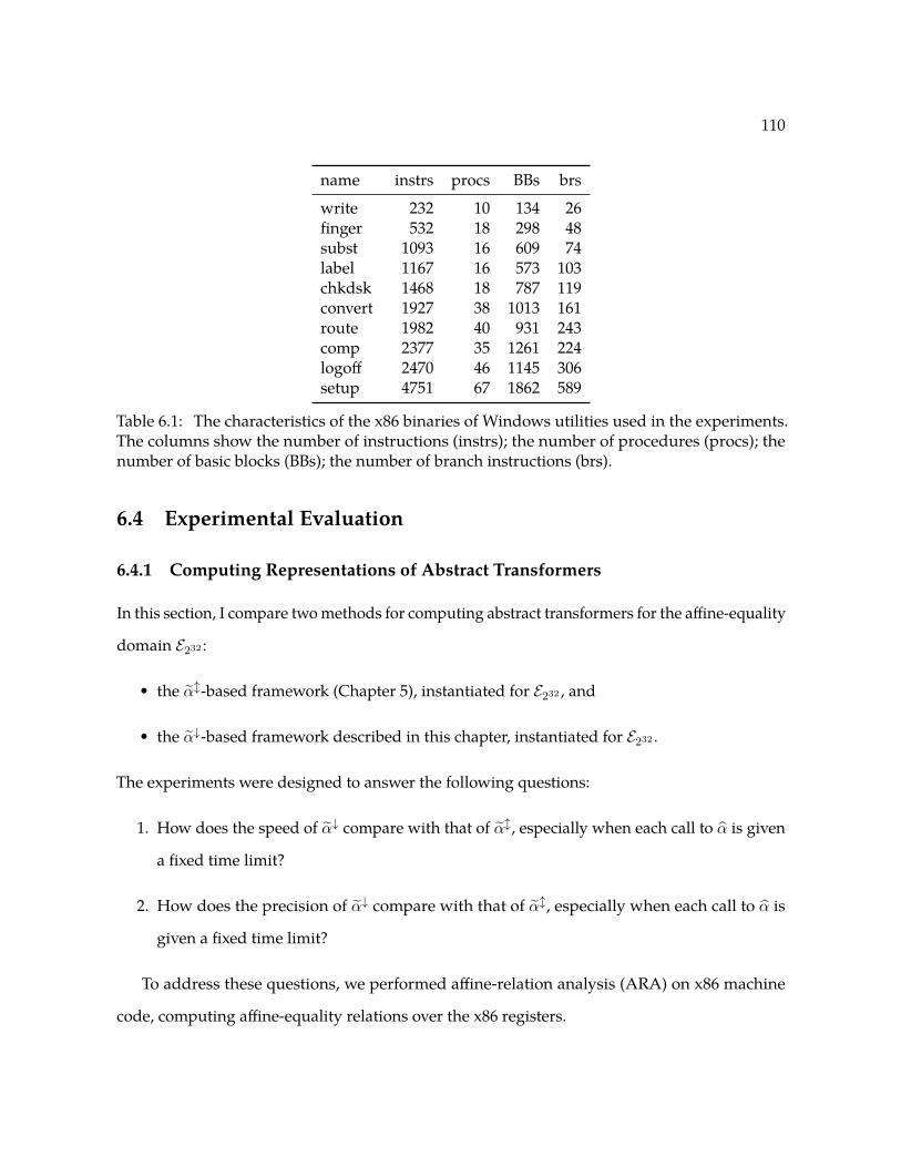
110
name instrs procs BBs brs
write 232 10 134 26finger 532 18 298 48subst 1093 16 609 74label 1167 16 573 103chkdsk 1468 18 787 119convert 1927 38 1013 161route 1982 40 931 243comp 2377 35 1261 224logoff 2470 46 1145 306setup 4751 67 1862 589
Table 6.1: The characteristics of the x86 binaries of Windows utilities used in the experiments.The columns show the number of instructions (instrs); the number of procedures (procs); thenumber of basic blocks (BBs); the number of branch instructions (brs).
6.4 Experimental Evaluation
6.4.1 Computing Representations of Abstract Transformers
In this section, I compare two methods for computing abstract transformers for the affine-equality
domain E232 :
• the αl-based framework (Chapter 5), instantiated for E232 , and
• the α↓-based framework described in this chapter, instantiated for E232 .
The experiments were designed to answer the following questions:
1. How does the speed of α↓ compare with that of αl, especially when each call to α is given
a fixed time limit?
2. How does the precision of α↓ compare with that of αl, especially when each call to α is
given a fixed time limit?
To address these questions, we performed affine-relation analysis (ARA) on x86 machine
code, computing affine-equality relations over the x86 registers.

111
αlt=∞ α
lt=1 α↓t=∞ α↓t=1
write 52.10 19.33 10.01 6.536finger 99.42 31.51 29.03 12.35subst 118.1 51.62 27.45 17.03label 89.84 57.13 28.00 18.72chkdsk 249.3 88.56 106.0 33.96route 438.7 124.1 95.56 43.89convert 212.4 98.02 83.56 34.82comp 588.6 149.3 105.9 46.78logoff 481.4 176.8 168.9 75.11setup 1318 358.7 476.5 177.7
Table 6.2: Time taken, in seconds, by the αl and α↓ algorithms for WPDS construction. Thesubscript is used to denote the time limit used for a single invocation of a call to α: t =∞ denotesthat no time limit was given, and t = 1 denotes that a time limit of 1 second was given. For eachbenchmark, the algorithm that takes the least time is highlighted in bold.
The experimental setup in this section differs slightly from that used in Sections 4.3 and 5.5
in the following two ways:
• The αl and α↓ algorithms are passed an over-approximation of the answer computed using
operator-by-operator reinterpretation.2 This scenario better reflects how α frameworks are
likely to be used in practice, and also highlights the fact that these two frameworks can
make use of an initial over-approximation. A (non-trivial) initial over-approximation aids
the Bilateral algorithm (αl) by guiding the set of abstract consequences it chooses.
• The set of benchmarks used in this experiment (Table 6.1) is a strict superset of the bench-
marks used in Sections 4.3 and 5.5.
Apart from the above two items, the rest of the experimental setup is the same as that used in
Sections 4.3 and 5.5.
Table 6.2 shows the time taken, in seconds, by the αl and α↓ algorithms for WPDS construction.
I also ran each of the algorithms with and without a total time limit on a single invocation of a
call to α. The subscript is used to denote the time limit used for a single invocation of a call to α:2Section 3.1.2 briefly describes the TSL system used for computing transformers via reinterpretation.

112
αlt=∞ better α↓t=1 better
than α↓t=1 than αlt=∞write 0% 11.54%finger 0% 12.50%subst 0% 12.16%label 0% 4.85%chkdsk 9.24% 0%route 6.17% 4.53%convert 0% 0%comp 0% 1.34%logoff 11.76% 10.78%setup 0% 4.70%
Table 6.3: Comparison of the degree of improvement gained by using αlt=∞ and α↓t=1 (measuredas the percentage of control points for which the inferred one-vocabulary affine relation inferredby one analysis was strictly more precise than that inferred by the other analysis).
t =∞ denotes that no time limit was given, and t = 1 denotes that a time limit of 1 second was
given. From Table 6.2, we see that α↓t = 1 is 7.5 times faster than αlt=∞, and 2.7 times faster than
αlt=1 (computed as the geometric mean). This table answers question 1 stated above.
To answer question 2, we compare the precision of the WPDS analysis when using αl with the
precision obtained using α↓. In particular, we compare the affine-relation invariants computed
by the α↓-based and αl-based analyses for each control point. Table 6.3 compares the precision
of αlt=∞ and α↓t=1. We see that α↓ computes precise invariants even when given a much smaller
time limit of 1 second. Though not shown in Table 6.3, the precision of αlt=1 was slightly worse
than αlt=∞, while the precision of α↓t=∞ was the same as that of α↓t=1. Increasing the depth of the
Dilemma Rule from k = 1 to k = 2 did not improve precision of α↓.
6.4.2 Checking Unsatisfiability of LRA formulas
The formula used in Example 6.3 is just one instance of a family of unsatisfiable LRA formu-
las (McMillan et al., 2009). Let χd = (ad < a0) ∧∧d−1i=0 ((ai < bi) ∧ (ai < ci) ∧ ((bi < ai+1) ∨ (ci <
ai+1))). The formula ψ in Example 6.3 is χ2; that is, the number of “diamonds” is 2 (see Fig-
ure 6.3(a)). These “diamond formulas” appear in the naive encoding of sequences of if-then-elses

113
Figure 6.7: Semilog plot of Z3 vs. α↓ on χd formulas.
in programs, for instance, when trying to compute the worst-case execution time (Henry et al.,
2014). We used the (LRA, Polyhedra) instantiation of our framework to check whether α(χd) = ⊥
for d = 1 . . . 25 using 1-assume. We ran this experiment on a single processor of a 16-core 2.4
GHz Intel Zeon computer running 64-bit RHEL Server release 5.7. The semilog plot in Figure 6.7
compares the running time of α↓ with that of Z3, version 3.2 (de Moura and Bjørner, 2008). The
time taken by Z3 increases exponentially with d, exceeding the timeout threshold of 1000 seconds
for d = 23. These measurements corroborate the results of a similar experiment conducted by
McMillan et al. (2009), where the reader can also find an in-depth explanation of Z3’s behavior
on this family of formulas.
On the other hand, the running time of α↓ increases linearly with d taking 0.78 seconds for
d = 25. The cross-over point is d = 12. In Example 6.3, we saw how two successive applications
of the Dilemma Rule suffice to prove that ψ is unsatisfiable. That explanation generalizes to χd:
d applications of the Dilemma Rule are sufficient to prove unsatisfiability of χd. The order in
which Boolean variables with unknown truth values are selected for use in the Dilemma Rule
has no bearing on this linear behavior, as long as no variable is starved from being chosen (i.e., a
fair-choice schedule is used). Each application of the Dilemma Rule is able to infer that ai < ai+1
for some i.
We do not claim that α↓ is always better than mature SMT solvers such as Z3. We do believe
that it represents another interesting point in the design space of SMT solvers, similar in nature

114
to the GDPLL algorithm (McMillan et al., 2009) and the k-lookahead technique used in the
DPLL(t) algorithm (Bjørner and de Moura, 2008).
6.5 Related Work
In the context of checking functional equivalence of sequential circuits, van Eijk (1998) and Bjesse
and Claessen (2000) present symbolic-abstraction algorithms for the abstract domain of Boolean
equalities. Van Eijk performs symbolic abstraction using BDDs. Bjesse and Claessen convert
van Eijk’s algorithm to use Stålmarck’s method (Sheeran and Stålmarck, 2000) instead of BDDs.
Furthermore, Bjesse and Claessen (2000) extend Stålmarck’s method from using equivalences
between variables to implications between variables.
Recent work has also explored connections between abstract interpretation and decision
procedures (D’Silva et al., 2012, 2013; Haller, 2013; D’Silva et al., 2014). In particular, D’Silva et al.
(2013) generalize the algorithm for Conflict Driven Clause Learning used in SAT solvers to solve
the lattice-theoretic problem of determining if an additive transformer on a Boolean lattice is
always bottom. In contrast, our algorithms address a broader class of problems. Our algorithms
apply to non-Boolean lattices. Moreover, provided there are no timeouts, our algorithms are
capable of discovering if the most-precise answer is ⊥. However, they are also useful when
the most-precise answer is not ⊥; in particular, our algorithms can be used to compute best
transformers. Furthermore, as described in Chapter 7, our algorithms can be used to solve the
BII problem (assuming no timeouts), and even when there are timeouts, they generate inductive
program invariants. Our work and that of D’Silva et al. were performed independently and
contemporaneously.
6.6 Chapter Notes
I first came across Stålmarck’s method in Harrison (2009). The fact that there was a merge of
proof branches involved was what stuck with me. Plenty of thinking and discussions with Tom
115
resulted in the simple insight that the intersection of constraints at the merge of the Dilemma
Rule corresponds to the join of abstract values.
I spent a considerable amount of time trying to engineer a pure Stålmarck-based SAT/SMT
solver that would be competitive with state-of-the-art solvers. Alas the tremendous progress in
SAT solvers, such as variable-selection heuristics, and conflict-driven clause learning (CDCL),
and my inadequate engineering skills forced me to abandon this approach; see Thakur and Reps
(2012) for some preliminary experiments using my earlier prototype, and Chapter 10 for a more
practical design that incorporates the best of the Stålmarck-style approach and the DPLL/CDCL
approach.
One takeaway from my earlier prototype was the need for implementations of abstract do-
mains that scaled as the number of variables increased; in my experience, the abstract operations
of join and meet became prohibitively expensive when the number of variables was greater than
50.

116
Chapter 7
Computing Best Inductive Invariants
In Chapters 4, 5, and 6, symbolic abstraction was used to compute best abstract transformers
for a sequence of statements. In this chapter, I show how symbolic abstraction can be used to
compute best inductive invariants for an entire program.
Let C be the concrete domain that describes the collecting semantics of the program. For
a concrete transformer τ , let Post[τ ] : C → C denote the operator that applies the concrete
transformer. A set of invariants {Ik} are said be inductive with respect to a set of transformers
{τij} if, for all i and j, Post[τij ](JIiK) ⊆ JIjK, where JIkK ∈ C denotes the meaning of Ik.
The choice of a particular abstract domain A fixes a limit on the precision of the invariants
identified by an analysis. If {Ik} is a set of inductive invariants, and Ij ∈ A for each single
member Ij of {Ik}, then the set of invariants {Ik} are said to be inductive A-invariants. (For
brevity, I also refer to a single member Ij of {Ik} as an inductive A-invariant.) Furthermore,
a most-precise inductive A-invariant exists: Post[τ ] is monotonic in C; given two A-invariants,
we can take their meet; thus, provided A is a meet semi-lattice, the most-precise inductive
A-invariant exists. (On the other hand, computing the most preciseA-invariant at a program point,
defined as the abstraction of the collecting semantics at that point, is generally infeasible.)
117
In summary, the best inductive invariant (BII) problem can be stated as follows:
Given program P , and an abstract domain A, find the most-precise inductive A-
invariant for P .
BII is clearly an important problem because it represents the limit of obtainable precision for
a given abstract domain. The key insights behind our approach are:
• The BII problem reduces to the problem of applying Post.
• The problem of applying Post reduces to the problem of symbolic abstraction.
Because the symbolic-abstraction approach solves the BII problem (in the absence of timeouts), it
can obtain more precise results than more conventional approaches to implementing abstract in-
terpreters. In particular, the symbolic-abstraction approach can identify invariants and procedure
summaries that are more precise than the ones obtained by more conventional approaches.
Not only does the work provide insight on fundamental limits in abstract interpretation,
the algorithms that I present are also practical. Santini is an invariant-generation tool based on
the principles of symbolic abstraction. Santini uses the predicate-abstraction domain that can
infer arbitrary Boolean combinations of a given set of predicates. The implementation of the
abstract domain was simple: just 1200 lines of C# code. We then compared the performance of
Santini with Houdini (Flanagan and Leino, 2001), which is a well-established tool that infers
only conjunctive invariants from a given set of predicates. We ran the Corral model checker (Lal
et al., 2012) using invariants supplied by Houdini and Santini. For 19 examples for which Corral
gave an indefinite result using Houdini-supplied invariants, invariants discovered using Santini
allowed Corral to give a definite result in 9 cases (47%); see (Thakur et al., 2013, Section 5).
This experiment shows that symbolic abstraction provides a powerful tool that can be used
to implement automatically a correct and precise invariant generator that uses an expressive
abstract domain. The other instantiation of our BII framework is based on WALi (Kidd et al.,
2007), a tool for solving program-analysis problems using an abstract domain, which we have
used to perform machine-code analysis (Thakur et al., 2013, Section 5).

118
7.1 Basic Insights
The following observation states how the most-precise inductive A-invariant can be computed:
Observation 7.1. Let program P consist of (i) nodes N = {ni} with enter node n1, (ii) edges
EP = {ni → nj}, and (iii) a concrete-state transformer τi,j associated with each edge ni → nj .
Let A be an abstract domain. The best inductive invariant (BII) for P that is expressible in A is
the least fixed-point of the equation system
V1 = a1 Vj =⊔ni→nj∈EP
Post[τi,j ](Vi), (7.1)
where a1 is the best value in A that over-approximates the set of allowed input states at the enter
node n1. (“Best” means best with respect to A.)
As a corollary of Observation 7.1, we have
Observation 7.2. When the least solution to Equation (7.1) can be obtained algorithmically, e.g.,
by Kleene iteration in an abstract domain with no infinite ascending chains, the BII problem
reduces to the problem of applying Post.
The precision obtained from a solution to BII depends on the set of “observation points” (or,
equivalently the equation system being solved). For instance, in Example 3.6, the strawman
solution does compute the best inductive A-invariant if the intermediate point between τ1 and τ2
is observable. Example 3.6 shows that, from the standpoint of precision, the fewer observation
points, the better. As with many methods in automatic program analysis and verification, our
method normally requires that each loop be cut by at least one observation point. Thus, the set
of loop headers would be a natural choice for the set of observation points. The take-away from
this discussion is that it can be desirable to have a procedure that is capable of applying Post for
an arbitrary loop-free sequence of instructions.
Equation (7.1) has a conventional form, but is non-standard because it uses the application of
the most-precise abstract transformer Post[τi,j ], whereas most work on abstract interpretation

119
uses less-precise abstract transformers. For instance, some systems only support the state trans-
formations of a restricted modeling language—e.g., affine programs (Cousot and Halbwachs,
1978; Müller-Olm and Seidl, 2004) or Boolean programs (Ball and Rajamani, 2000). Transfor-
mations outside the modeling language are over-approximated very coarsely. For example,
for an assignment statement “x := e” in the original program, if e is an expression that uses
any non-modeled operator, the statement is modeled as “x := ?” or, equivalently, “havoc(x)”.
(That is, after “x := e” executes, x can hold any value.) This translation from a program to the
program-modeling language already involves some loss of precision.
In contrast, the application of Post[τi,j ] in Equation (7.1) always incorporates the full concrete
semantics of τi,j (i.e., without an a priori abstraction step).
7.2 Best Inductive Invariants and Intraprocedural Anaysis
Figure 7.1(a) shows an example program that illustrates finding the best inductive invariant when
the abstract domain is the affine-equalities domain E232 . We concentrate on lines 1, 6, and 12.
Figure 7.1(b) depicts the dependences in the equation system over node-variables {V1, V6, V12}.
Figure 7.1(c) gives formulas for the transition relations among {V1, V6, V12}. The remainder of
this section illustrates how to solve the BII problem for the following equation system, which
corresponds to Figures 7.1(b) and 7.1(c):
V1 = >
V6 = Post[τ1,6](V1) t Post[τ6,6](V6)
V12 = Post[τ6,12](V6)

120
(a)
(1) // Initialize(2) a = read_input();(3) b = a;(4) x = 0;(5) y = 0;(6) while (*) { // Loop invariant: a==b && x==y(7) a = a+2;(8) b = (x==y) ? b+2 : read_input();(9) x = x+1;(10) y = (a==b) ? y+1 : read_input();(11) }(12) . . . // Exit invariant: a==b && x==y
(b)
V1
V12
V6
τ1,6
τ6,6τ6,12
τ1,6def= b′ = a′ ∧ x′ = 0 ∧ y′ = 0
(c) τ6,6def=
a′ = a+ 2∧ (x = y)⇒(b′ = b+ 2)∧ x′ = x+ 1∧ (a′ = b′)⇒(y′ = y + 1)
τ6,12
def= a′ = a ∧ b′ = b ∧ x′ = x ∧ y′ = y
Figure 7.1: (a) Example program. (b) Dependences among node-variables in the program’s equa-tion system (over node-variables {V1, V6, V12}). (c) The transition relations among {V1, V6, V12}(expressed as formulas).
It is convenient to rewrite these equations as
V1 = >
V6 = V6 t Post[τ1,6](V1) t Post[τ6,6](V6) (7.2)
V12 = V12 t Post[τ6,12](V6)
Solving the BII Problem from Below. In the most basic approach to solving the BII problem,
we assume that we have an essentially standard fixed-point solver that performs chaotic iteration.
The method will create successively better under-approximations to the solution, until it finds
a fixed point, which will also be the best inductive invariant. We illustrate the algorithm on
Equation (7.2).1
1 We write abstract values in Courier typeface (e.g., [a = b, x = 0, y = 0] or [a′ = b′, x′ = 0, y′ = 0]are pre-state and post-state abstract values, respectively); concrete state-pairs in Ro-man typeface (e.g.,
[a 7→ 42, b 7→ 27, x 7→ 5, y 7→ 19, a′ 7→ 17, b′ 7→ 17, x′ 7→ 0, y′ 7→ 0
]); and ap-
proximations to BII solutions as mappings from node-variables to abstract values (e.g.,〈V1 7→ >,V6 7→ [a = b, x = 0, y = 0],V12 7→ [a = 28,b = 28, x = 35, y = 35]〉).

121
What is special, compared to standard equation solvers, is that each application of the
right-hand side of an equation in Equation (7.2)—defined by the corresponding formula in
Figure 7.1(c)—is given the best-transformer interpretation by means of a function Post for applying
the best abstract transformer. That is, Post satisfies Post[τ ](a) = (α ◦ Post[τ ] ◦ γ)(a). A specific
instance of Post is the function Post↑, given as Algorithm 8.
Figure 7.2 shows a possible chaotic-iteration sequence when a BII solver is invoked to find
the best inductive affine-equality invariant for Equation (7.2), namely,
〈V1 7→ >,V6 7→ [a = b, x = y],V12 7→ [a = b, x = y]〉.
Note that this abstract value corresponds exactly to the loop-invariant and exit-invariant shown
in the comments on lines 6 and 12 of Figure 7.1(a). Moreover, the same abstract value would be
arrived at no matter what sequence of choices is made during chaotic iteration to find the least
fixed-point of Equation (7.2).
One such sequence is depicted in Figure 7.2, where three chaotic-iteration steps are performed
before the least fixed point is found. The three steps propagate information from V1 to V6; from
V6 to V6; and from V6 to V12, respectively. (At this point, to discover that chaotic iteration has
quiesced, the solver would have to do some additional work, which we have not shown because
it does not provide any additional insight on how BII problems are solved.)
The Value of a Bilateral Algorithm. Post↑
is not resilient to timeouts. A query to the SMT
solver—or the cumulative time for Post↑—might take too long, in which case the only answer
that is safe for Post↑
to return is > (line 5 of Algorithm 8). To remedy this situation, we use a
bilateral algorithm for Post. Algorithm 15 (Chapter 5) shows our bilateral algorithm for Post,
called Postl.
Figure 7.3 shows a possible trace of Iteration 2 from Figure 7.2 when the call to Post↑
(Al-
gorithm 8) is replaced by a call to Postl
(Algorithm 15). Note how a collection of individual,
non-trivial, upper-bounding constraints are acquired on the second, third, and fifth calls to
AbstractConsequence: [x′ = 1], [y′ = 1], and [a′ = b′], respectively. By these means, upper′works

122
Initialization: ans := 〈V1 7→ >,V6 7→ ⊥,V12 7→ ⊥〉Iteration 1: V6 := V6 t Post
↑[τ1,6](V1)
= ⊥ t Post↑[τ1,6](>)
lower′ := ⊥〈S, S′〉 := Model(true ∧ τ1,6 ∧ ¬γ(⊥))
=[a 7→ 42, b 7→ 27, x 7→ 5, y 7→ 99,a′ 7→ 17, b′ 7→ 17, x′ 7→ 0, y′ 7→ 0
]// A satisfying concrete// state-pair
lower′ := ⊥ t [a′ = 17, b′ = 17, x′ = 0, y′ = 0]〈S, S′〉 := Model(true ∧ τ1,6 ∧ ¬γ([a′ = 17,b′ = 17, x′ = 0, y′ = 0]))
=[a 7→ 73, b 7→ 2, x 7→ 15, y 7→ 19,a′ 7→ 28, b′ 7→ 28, x′ 7→ 0, y′ 7→ 0
]// A satisfying concrete// state-pair
lower′ := [a′ = 17, b′ = 17, x′ = 0, y′ = 0] t [a′ = 28,b′ = 28, x′ = 0, y′ = 0]v′ := [a′ = b′, x′ = 0, y′ = 0]V6 := ⊥ t [a = b, x = 0, y = 0] = [a = b, x = 0, y = 0]ans := 〈V1 7→ >,V6 7→ [a = b, x = 0, y = 0],V12 7→ ⊥〉
Iteration 2: V6 := V6 t Post↑[τ6,6](V6)
= [a = b, x = 0, y = 0] t Post↑[τ6,6]([a = b, x = 0, y = 0])
lower′ := ⊥〈S, S′〉 := Model(γ([a = b, x = 0, y = 0]) ∧ τ6,6 ∧ ¬γ(⊥))
=[a 7→ 56, b 7→ 56, x 7→ 0, y 7→ 0,a′ 7→ 58, b′ 7→ 58, x′ 7→ 1, y′ 7→ 1
]// A satisfying concrete// state-pair
lower′ := ⊥ t [a′ = 58, b′ = 58, x′ = 1, y′ = 1]〈S, S′〉 := Model(γ([a = b, x = 0, y = 0]) ∧ τ6,6 ∧ ¬γ([a′ = 58, b′ = 58, x′ = 1, y′ = 1]))
=[a 7→ 16, b 7→ 16, x 7→ 0, y 7→ 0,a′ 7→ 18, b′ 7→ 18, x′ 7→ 1, y′ 7→ 1
]// A satisfying concrete// state-pair
lower′ := [a′ = 58, b′ = 58, x′ = 1, y′ = 1] t [a′ = 18,b′ = 18, x′ = 1, y′ = 1]v′ := [a′ = b′, x′ = 1, y′ = 1]V6 := [a = b, x = 0, y = 0] t [a = b, x = 1, y = 1] = [a = b, x = y]ans := 〈V1 7→ >,V6 7→ [a = b, x = y],V12 7→ ⊥〉
Iteration 3: V12 := V12 t Post↑[τ6,12](V6)
= ⊥ t Post↑[τ6,12]([a = b, x = y])
lower′ := ⊥〈S, S′〉 := Model(γ([a = b, x = y]) ∧ τ6,6 ∧ ¬γ(⊥))
=[a 7→ 17, b 7→ 17, x 7→ 99, y 7→ 99,a′ 7→ 17, b′ 7→ 17, x′ 7→ 99, y′ 7→ 99
]// A satisfying concrete// state-pair
lower′ := ⊥ t [a′ = 17, b′ = 17, x′ = 99, y′ = 99]〈S, S′〉 := Model(γ([a = b, x = y]) ∧ τ6,6 ∧ ¬γ([a′ = 17,b′ = 17, x′ = 99, y′ = 99]))
=[a 7→ 28, b 7→ 28, x 7→ 35, y 7→ 35,a′ 7→ 28, b′ 7→ 28, x′ 7→ 35, y′ 7→ 35
]// A satisfying concrete// state-pair
lower′ := [a′ = 17, b′ = 17, x′ = 99, y′ = 99] t [a′ = 28,b′ = 28, x′ = 35, y′ = 35]v′ := [a′ = b′, x′ = y′]V12 := ⊥ t [a = b, x = y] = [a = b, x = y]ans := 〈V1 7→ >,V6 7→ [a = b, x = y],V12 7→ [a = b, x = y]〉
Fixed Point!
Figure 7.2: A possible chaotic-iteration sequence when a BII solver is invoked to find the bestinductive affine-equality invariant for Equation (7.2). The parts of the trace enclosed in boxesshow the actions that take place in calls to Algorithm 8 (Post
↑). (By convention, primes are
dropped from the abstract value returned from a call on Post↑.)

123
V6 := V6 t Postl[τ6,6](V6)
= [a = b, x = 0, y = 0] t Postl[τ6,6]([a = b, x = 0, y = 0])
upper′ := >lower′ := ⊥
p′ := AbstractConsequence(⊥,>)= ⊥
〈S, S′〉 := Model(γ([a = b, x = 0, y = 0]) ∧ τ6,6 ∧ ¬γ(⊥))=
[a 7→ 56, b 7→ 56, x 7→ 0, y 7→ 0,a′ 7→ 58, b′ 7→ 58, x′ 7→ 1, y′ 7→ 1
]// A satisfying concrete// state-pair
lower′ := ⊥ t [a′ = 58, b′ = 58, x′ = 1, y′ = 1]p′ := AbstractConsequence([a′ = 58,b′ = 58, x′ = 1, y′ = 1],>)
= [x′ = 1]〈S, S′〉 := Model(γ([a = b, x = 0, y = 0]) ∧ τ6,6 ∧ ¬γ([x′ = 1]))
= Noneupper′ := > u [x′ = 1] = [x′ = 1]
p′ := AbstractConsequence([a′ = 58,b′ = 58, x′ = 1, y′ = 1], [x′ = 1])= [y′ = 1]
〈S, S′〉 := Model(γ([a = b, x = 0, y = 0]) ∧ τ6,6 ∧ ¬γ([y′ = 1]))= None
upper′ := [x′ = 1] u [y′ = 1] = [x′ = 1, y′ = 1]p′ := AbstractConsequence([a′ = 58,b′ = 58, x′ = 1, y′ = 1], [x′ = 1, y′ = 1])
= [a′ = 58]〈S, S′〉 := Model(γ([a = b, x = 0, y = 0]) ∧ τ6,6 ∧ ¬γ([a′ = 58]))
=[a 7→ 19, b 7→ 19, x 7→ 0, y 7→ 0,a′ 7→ 21, b′ 7→ 21, x′ 7→ 1, y′ 7→ 1
]// A satisfying concrete// state-pair
lower′ := [a′ = 58, b′ = 58, x′ = 1, y′ = 1] t [a′ = 21,b′ = 21, x′ = 1, y′ = 1]= [a′ = b′, x′ = 1, y′ = 1]
p′ := AbstractConsequence([a′ = b′, x′ = 1, y′ = 1], [x′ = 1, y′ = 1])= [a′ = b′]
〈S, S′〉 := Model(γ([a = b, x = 0, y = 0]) ∧ τ6,6 ∧ ¬γ([a′ = b′]))= None
upper′ := [x′ = 1, y′ = 1] u [a′ = b′]= [a′ = b′, x′ = 1, y′ = 1]
lower′ 6= upper′ = falsev′ := [a′ = b′, x′ = 1, y′ = 1]V6 := [a = b, x = 0, y = 0] t [a = b, x = 1, y = 1] = [a = b, x = y]ans := 〈V1 7→ >,V6 7→ [a = b, x = y],V12 7→ ⊥〉
Figure 7.3: A possible trace of Iteration 2 from Figure 7.2 when the call to Post↑
(Algorithm 8) isreplaced by a call to Post
l(Algorithm 15).
its way down the chain> A [x′ = 1] A [x′ = 1, y′ = 1] A [a′ = b′, x′ = 1, y′ = 1]. After each call to
AbstractConsequence, the abstract-consequence constraint is tested to see if it really is an upper
bound on the answer. For instance, the fourth call to AbstractConsequence returns [a′ = 58].

124
The assertion that [a′ = 58] is an upper-bounding constraint is refuted by the concrete state-pair
〈S, S′〉 =
a 7→ 19, b 7→ 19, x 7→ 0, y 7→ 0,
a′ 7→ 21, b′ 7→ 21, x′ 7→ 1, y′ 7→ 1
,which is used to improve the value of lower′.
The important point is that if Iteration 2 is taking too much time, Postl
can be stopped and
upper′ returned as the answer. In contrast, if Post↑
is stopped because it is taking too much
time, the only safe answer that can be returned is >. The “can-be-stopped-anytime” property of
Postl
can make a significant difference in the final answer. For instance, suppose that Post↑
and
Postl
both stop early during Iteration 2 (Figures 7.2 and 7.3, respectively), and that Postl
returns
[x = 1, y = 1], whereas Post↑
returns >. Assuming no further timeouts take place during the
evaluation of Equation (7.2), the respective final answers would be
Post↑
: 〈V1 7→ >,V6 7→ >,V12 7→ >〉
Postl
: 〈V1 7→ >,V6 7→ [x = y],V12 7→ [x = y]〉
Because of the timeout, the answer computed by Postl
is not the best inductive affine-equality
invariant; however, the answer establishes that the equality constraint [x = y] holds at both lines 6
and 12 of Figure 7.1(a).
Attaining the Best Inductive A-Invariant
Lemma 7.3. The least fixed-point of Equation (7.1) (the best A-transformer equations of a transition
system) is the best inductive invariant expressible in A.
Corollary 7.4. Applying an equation solver to the best A-transformer equations, using either Post↑
or
Postl
to evaluate equation right-hand sides, finds the best inductive A-invariant if there are no timeouts
during the evaluation of any right-hand side.

125
7.3 Best Inductive Invariants and Interprocedural Analysis
This section presents a method for solving the BII problem for multi-procedure programs. Our
framework is similar to the so-called “functional approach” to interprocedural analysis of Sharir
and Pnueli (1981) (denoted by SP), which works with an abstract domain that abstracts transition
relations. For instance, our approach
• also uses an abstract domain that abstracts transition relations, and
• creates a summary transformer for each reachable procedure P , which over-approximates
the transition relation of P .
However, to make the symbolic-abstraction approach suitable for interprocedural analysis,
the algorithm uses a generalization of Post, called Compose[τ ](a), where τ ∈ L[−→v ;−→v ′] and
a ∈ A[−→v ;−→v ′] both represent transition relations over the program variables −→v . The goal of
Compose[τ ](a) is to create an A[−→v ;−→v ′] value that is the best over-approximation of a’s action
followed by τ ’s action. Furthermore, instead of Equation (7.1), the least solution to Equations (7.3)–
(7.7) below is found, where each application of the right-hand side of an equation is given the
best-transformer interpretation—in this case, by means of Compose.
A program is defined by a set of procedures Pi, 0 ≤ i ≤ K, and represented by an interproce-
dural control-flow graph G = (N,F ). G consists of a collection of intraprocedural control-flow
graphs G1, G2, . . . , GK , one of which, G main, represents the program’s main procedure. The
node set Ni of Gi = (Ni, Fi) is partitioned into five disjoint subsets: Ni = Ei ]Xi ] Ci ]Ri ] Li.
Gi contains exactly one enter node (i.e., Ei = {ei}) and exactly one exit node (i.e., Xi = {xi}). A
procedure call in Gi is represented by two nodes, a call node c ∈ Ci and a return-site node r ∈ Ri,
and has two edges: (i) a call-to-enter edge from c to the enter node of the called procedure, and
(ii) an exit-to-return-site edge from the exit node of the called procedure to r. The functions call
and ret record matching call and return-site nodes: call(r) = c and ret(c) = r. It is assumed that
an enter node has no incoming edges except call-to-enter edges.

126
φ(e main) = Id|a1 a1 ∈ A describes the set of initial stores at e main (7.3)
φ(ep) = Id|a ep ∈ E, p 6= main, and a =⊔
c∈C, c calls pVc (7.4)
φ(n) =⊔
m→n∈F
Compose[τm,n](φ(m)) for n ∈ N , n 6∈ (R ∪ E) (7.5)
φ(n) = Compose[γ(φ(xq))](φ(call(n))) for n ∈ R, and call(n) calls q (7.6)
Vn = range(φ(n)) (7.7)
The equations involve two sets of “variables”: φ(n) and Vn, where n ∈ N . φ(n) is a partial
function that represents a summary of the transformation from eproc(n) to n. Id|a denotes the
identity transformer restricted to inputs in a ∈ A. The domain of φ(n) over-approximates the
set of reachable states at eproc(n) from which it is possible to reach n; the range of φ(n) over-
approximates the set of reachable states at n. Vn’s value equals the range of φ(n).
Composel
is essentially identical to Algorithm 15, except that in line 5, Composel
performs
a query using a three-state formula,
〈S, S′, S′′〉 ← Model(γ[−→v ,−→v ′](a) ∧ τ[−→v ′,−→v ′′] ∧ ¬γ[−→v ,−→v ′′](p′)),
and in line 11, Composel
applies a two-state version of β to S and S′′, dropping S′ completely:
lower′ ← lower′ t β(S, S′′). ( Compose↑
is defined similarly.)
An important difference between our algorithm and the SP algorithm is that in our algorithm,
the initial abstract value for the enter node ep for procedure p is specialized to the reachable
inputs of p (see Equation (7.4)). In the SP algorithm, φ(ep) is always set to Id. Figure 7.4 illustrates
the effect on the inferred abstract post-condition at xp of specializing the abstract pre-condition
at enter node ep. The abstract domain used in Figure 7.4 is the domain of affine equalities over
machine integers E232 . With that domain, it is possible to express that a 32-bit variable x holds
an even number: 231x = 0. Consequently, the initial abstract value for enter node ehalve is the

127
(1) main() {(2) x = read_input();(3) while (x != 1) {(4) if (even(x)) halve();(5) else increase();(6) }(7) }
(8) void halve() {(9) x = x � 1;(10) }(11)(12) void increase() {(13) x = 3*x + 1;(14) }
Abstract value at enter node epId Id|a, where a =
⊔c∈C, c calls p Vc
halve pre-condition (ehalve) x′ = x 231x = 0 ∧ x′ = xpost-condition (xhalve) > 231x = 0 ∧ x− 2x′ = 0
increase pre-condition (eincrease) x′ = x 231x = 1 ∧ x′ = xpost-condition (xincrease) x′ = 3x+ 1 231x = 1 ∧ 231x′ = 0 ∧ x′ = 3x+ 1
Figure 7.4: The effect of specializing the abstract pre-condition at enter node ep, and the resultingstrengthening of the inferred abstract post-condition. (The abstract domain is the domain ofaffine equalities E232 .)
identity relation, constrained so that x is even. Similarly, the initial abstract value for enter node
eincrease is the identity relation, constrained so that x is odd.
Note that the abstract value at the exit point xp of a procedure p serves as a procedure
summary—i.e., an abstraction of p’s transition relation. Figure 7.4 shows that by giving halve
and increase more precise abstract values at the respective enter nodes, more precise procedure
summaries at the respective exit points are obtained. In particular, for halve, the constraint
x−2x′ = 0 provides a good characterization of the effect of a right-shift operation, but only when
x is known to be even (cf. the entries for halve’s post-condition in columns 3 and 4 of Figure 7.4).
7.4 Related Work
Houdini (Flanagan and Leino, 2001) is the first algorithm that I am aware of that solves a version
of the BII problem. The paper on Houdini does not describe the work in terms of abstract
interpretation. Santini (Thakur et al., 2013, Section 5) was directly inspired by Houdini, as an
effort to broaden Houdini’s range of applicability.

128
Yorsh et al. (2006) introduced a particularly interesting technique. Their algorithm for the BII
problem can be viewed as basically solving Equation (7.1) using Post↑. However, they observed
that it is not necessary to rely on calls to an SMT solver for all of the concrete states used by
Post↑; instead, they used concrete execution of the program as a way to generate concrete states
very cheaply. If for some program point q of interest they have state-set Sq, they obtain an
under-approximation for the abstract value Vq by performing Vq = t{β(σ) | σ ∈ Sq}. This idea
is similar in spirit to the computation of candidate invariants from execution information by
Daikon (Ernst et al., 2007). Because Postl
works simultaneously from below and from above,
the Yorsh et al. heuristic can be used to improve the speed of convergence of lower′ in line 11 of
Algorithm 15.
If we think of τ = 〈. . . , τi,j , . . .〉 as a monolithic transformer, an alternative way of stating the
objective of intraprocedural BII is as follows:
• Given a concrete transformer τ and an abstract value a ∈ A that over-approximates the set
of initial states, apply the best abstract transformer for τ∗ to a (i.e., apply Post[τ∗](a)).
This problem was the subject of a recent technical report by Garoche et al. (2012).
7.5 Chapter Notes
Extending the results of “best abstract transformers” to “best inductive invariant” appeared
daunting at first. Some amount of head scratching resulted in the simple observation that the
BII problem reduces to the problem of applying Post.
The Santini tool, which incorporates the ideas described in this chapter, was developed by
Akash Lal of Microsoft Research. Because I had little to do with the implementation of this
tool and the running of the experiments, I have omitted these experimental results from this
thesis. The curious reader is encouraged to read about Santini and its application in the Corral
verification tool in Thakur et al. (2013).

129
Chapter 8
Bit-Vector Inequality Domain
In this chapter, I describe how symbolic abstraction enables us to define a new abstract do-
main, called the Bit-Vector Inequality (BVI) domain, that addresses the following challenges:
(1) identifying affine-inequality invariants while handling overflow in arithmetic operations
over bit-vector data-types, and (2) holding onto invariants about values in memory during
machine-code analysis.
Need for bit-vector invariants. The polyhedral domain (Cousot and Halbwachs, 1978) is capable
of expressing relational affine inequalities over rational (or real) variables. However, the native
machine-integer data-types used in programs (e.g., int, unsigned int, long, etc.) perform
bit-vector arithmetic, and arithmetic operations wrap around on overflow. Thus, the underlying
point space used in the polyhedral domain does not faithfully model bit-vector arithmetic, and
consequently the conclusions drawn from an analysis based on the polyhedral domain are
unsound, unless special steps are taken (Simon and King, 2007).
Example 8.1. The following C-program fragment incorrectly computes the average of two int-valued variables (Bloch, 2014):
unsigned i n t low , high , mid ;assume (0 <= low <= high ) ;mid = ( low + high ) /2;a s s e r t (0 <= low <= mid <= high ) ;

130
A static analysis based on polyhedra would draw the unsound conclusion that the assertion
always holds. In particular, assuming 32-bit ints, when the sum of low and high is greater
than 232 − 1, the sum overflows to a negative value, and the resulting value of mid is negative.
Consequently, there exist runs in which the assertion fails. These runs are overlooked when the
polyhedral domain is used for static analysis because the domain fails to take into account the
bit-vector semantics of program variables. �
The problem that we wish to solve is not one of merely detecting overflow—e.g., to restrain an
analyzer from having to explore what happens after an overflow occurs. On the contrary, our
goal is to be able to track soundly the effects of arithmetic operations, including wrap-around
effects of operations that overflow. This ability is useful, for instance, when analyzing code
generated by production code generators, such as dSPACE TargetLink (dSPACE, 2014), which
use the “compute-through-overflow” technique (Garner, 1978). Furthermore, clever idioms
for bit-twiddling operations, such as the ones explained in Warren (2003), sometimes rely on
overflow.
Challenges in dealing with bit-vectors. The ideas used in designing an inequality domain for
reals do not carry over to one designed for bit-vectors. First, in bit-vector arithmetic, additive
constants cannot be cancelled on both sides of an inequality, as illustrated in the following
example.
Example 8.2. Let x and y be 4-bit unsigned integers. Figures 8.1(a) and 8.1(b) depict the solutions
in bit-vector arithmetic of the inequalities x+ y + 4 ≤ 7 and x+ y ≤ 3, respectively. Although
x+y+4 ≤ 7 and x+y ≤ 3 are syntactically quite similar, their solution spaces are quite different.
In particular, because of wrap-around of values computed on the left-hand sides using bit-vector
arithmetic, one cannot just subtract 4 from both sides to convert the inequality x+ y+ 4 ≤ 7 into
x+ y ≤ 3. �
Second, in bit-vector arithmetic, positive constant factors cannot be cancelled on both sides
of an inequality; for example, if x and y are 4-bit bit-vectors, then (4, 4) is in the solution set of
2x+ 2y ≤ 4, but not of x+ y ≤ 2.

131
15 + + + + + + + +14 + + + + + + + +13 + + + + + + + +12 + + + + + + + +11 + + + + + + + +10 + + + + + + + +
9 + + + + + + + +8 + + + + + + + +7 + + + + + + + +6 + + + + + + + +5 + + + + + + + +4 + + + + + + + +3 + + + + + + + +2 + + + + + + + +1 + + + + + + + +0 + + + + + + + +
0 1 2 3 4 5 6 7 8 9 10 11 12 13 14 15(a) x+ y + 4 ≤ 7
15 + + + +14 + + + +13 + + + +12 + + + +11 + + + +10 + + + +
9 + + + +8 + + + +7 + + + +6 + + + +5 + + + +4 + + + +3 + + + +2 + + + +1 + + + +0 + + + +
0 1 2 3 4 5 6 7 8 9 10 11 12 13 14 15(b) x+ y ≤ 3
Figure 8.1: Each + represents a solution of the indicated inequality in 4-bit unsigned bit-vectorarithmetic.
Recent work has developed several abstract domains of relational affine equalities over vari-
ables that hold machine integers (Müller-Olm and Seidl, 2005; King and Søndergaard, 2010;
Elder et al., 2011).1 These domains do account for wrap-around on overflow. With respect to
their analysis capabilities, the drawback of these domains is that they are unable to identify
inequality invariants.
While some simple domains do exist that are capable of representing certain kinds of inequal-
ities over bit-vectors (e.g., intervals with a congruence constraint, sometimes called “strided-
intervals” (Reps et al., 2006; Sen and Srikant, 2007; Balakrishnan and Reps, 2010)), such domains1The bit-vector affine-equalities domain E2w has been used in this thesis in Sections 4.3, 5.5, and 6.4.1.

132
are non-relational domains. That is, they are not capable of expressing relations among several
variables.
Challenges when dealing with memory. When analyzing machine-code, memory is usually
modeled as a flat array. When analyzing Intel x86 machine code, for instance, memory is modeled
as a map from 32-bit bit-vectors to 8-bit bit-vectors. Consequently, an analysis has to deal with
complications arising from the little-endian addressing mode and aliasing, as illustrated in the
next example.
Example 8.3. Consider the following machine-code snippet:
mov eax, [ebp]mov [ebp+2], ebx
The first instruction loads the four bytes pointed to by register ebp into the 32-bit register eax.
Suppose that the value in register ebp is A. After the first instruction, the bytes of eax contain, in
least-significant to most-significant order, the value at memory location A, the value at location
A+ 1, the value at location A+ 2, and the value at location A+ 3. The second instruction stores
the value in register ebx into the memory pointed to by ebp+2. Due to this instruction, the values
at memory locations A+ 2 through A+ 5 are overwritten, after which the value in register eax
no longer equals (the little-endian interpretation of) the bytes in memory pointed to by ebp. �
The contribution of this chapter can be summarized as follows:
• I describe the design and implementation of the BVI abstract domain, which is capable of
expressing affine-inequality invariants among bit-vector data-types, as well as handling
invariants about values in memory during machine-code analysis.
Section 8.2 presents related work. The presentation of an experimental evaluation of the BVI
domain is postponed until Chapter 9, where it can be found in Section 9.4

133
8.1 The BVI Abstract Domain
In this section, I present the intuition and formalism for the design and implementation of the
BVI abstract domain.
Abstract-Domain Vocabulary. For a given family of abstract domains A, A[V ] denotes the
specific instance of A that is defined over vocabulary V . Usually, the standard vocabulary used
to define an abstract domain is the set of program variables. For instance, in Section 5.5 we used
the abstract domain E232 [R], where R was the set of all 32-bit x86 registers; that is, E232 [R] is
the bit-vector affine-equalities domain E232 defined over the vocabulary of 32-bit x86 registers.
Consequently, E232 [R] is capable of expressing invariants among members of R.
Key Insights. The key insights behind the design of the BVI are:
• We extend the standard vocabulary of an abstract domain with view expressions, which are
w-bit terms expressed in some logic L. Thus, view expressions are capable of holding onto
richer constraints about the program state than the unenriched abstract domain alone.
• We construct the BVI domain as a reduced product between the bit-vector affine-equality
domain E2w and the bit-vector interval domain I2w .
• We use symbolic abstraction to implement precise versions of the abstract-domain opera-
tions for BVI.
Cousot et al. (2011b) use the term observables for view expressions. They also define the ob-
servational reduced product, which, in essence, is a reduced product of abstract domains those
vocabularies have been extended with observables.
I will illustrate each of the concepts listed in the key insights above using examples.
Example 8.4. This example illustrates how view expressions enable the abstract domain I2w to
express inequality constraints, and constraints over memory.
Let P ≡ {x, y, z} be the standard vocabulary consisting of 32-bit program variables x, y, and
z. Let t1 ≡ 2x+ 3y be a 32-bit term view expression. Let T ≡ P ∪ {t1} be the standard vocabulary
P extended with the view expression t1.

134
An element of I232 [P ] is able to only express a non-relational constraint between x, y, and
z. On the other hand, the abstract value I1 ≡[t1 7→ [0, 5]
]∈ I232 [T ] expresses the relational
bit-vector inequality constraint 0 ≤ 2x+ 3y ∧ 2x+ 3y ≤ 5.
To express invariants on values in memory (for machine-code analysis), we can add a view
expression that holds onto the values in memory. I use [e] to denote the 32-bit value at the
address e accessed using little-endian addressing. Let m1 ≡ [x + 2], m2 ≡ ([y] + 2z), and
M ≡ P ∪ {t1,m1,m2}. The abstract domain I232 [M ] is capable of expressing bit-vector affine-
inequality constraints, as well as constraints on the values in memory. For instance, the element
I2 ≡[t1 7→ [0, 5],m1 7→ [1, 10],m2 7→ [42, 56]
]∈ I232 [M ] expresses the following relational
inequality constraint over program variables and the contents of memory:
0 ≤ 2x+ 3y ∧ 2x+ 3y ≤ 5
∧ 1 ≤ [x+ 2] ∧ [x+ 2] ≤ 10
∧ 42 ≤ [y] + 2z ∧ [y] + 2z ≤ 56
�
Example 8.5. In this example, I illustrate how computing a reduced product of E2w and I2w
improves precision.
Consider the abstract value I1 ≡[t1 7→ [0, 5]
]∈ I232 [T ] defined in Example 8.4. An abstract
value in E232 [T ] is capable to expressing any bit-vector affine-equality relation among elements
of T . Constructing the reduced product E232 [T ] ? I232 [T ] expands the set of inequalities that are
expressible. For instance, let E1 ≡ {2x = z} ∈ E232 [T ]. The pair 〈E1, I1〉 expresses the following
constraint: 2x = z ∧ 0 ≤ 2x + 3y ∧ 2x + 3y ≤ 5. Furthermore, 〈E1, I1〉 implies the inequality
0 ≤ z + 3y ∧ z + 3y ≤ 5, which cannot be expressed in the individual domains E232 [T ] and
I232 [T ]. �
The previous two examples paint a rather rosy picture—in particular, it appears as if all one
needs to do is add view expressions to be able to handle bit-vector inequality constraints. As the
next example illustrates, adding view expressions is only half the story; we require machinery
that is capable of interpreting the semantics of the view expressions.
135
Example 8.6. Consider the abstract domain E232 [T ], where the vocabulary T is defined in
Example 8.4. Let E1 ≡ {t1 = 8} ∈ E232 [T ], and E2 ≡ {x = 2, y = 3} ∈ E232 [T ]. We
now want to compute E1 u E2. If we compute the meet of E1 and E2 using the meet al-
gorithm described in Elder et al. (2011), we get {x = 2, y = 3, t1 = 8}. However, though
sound, this meet operation ignores the semantics of the view expression t1. In particular,
γ({x = 2, y = 3, t1 = 8}) = Jx = 2 ∧ y = 3 ∧ 2x+ 3y = 8K = ∅. Consequently, the semantic
reduction (Definition 3.7) of the meet of E1 and E2 should be ⊥; that is, ρ(E1 u E2) = ⊥.
This simple example illustrates the fact that existing approaches for performing abstract
operations, such as meet and join, are not capable of interpreting the complex view expressions.
Furthermore, if a view expression holds onto values in memory, then the abstract operations
need to reason about the theory of arrays (Bradley et al., 2006) to be precise. �
The solution to implementing precise abstract operations, such as meet and join, is to use
symbolic abstraction. For instance, in Example 8.6 we can compute the semantic reduction
of {x = 2, y = 3, t1 = 8} ∈ E232 [T ], which is ⊥, using symbolic abstraction (Section 3.2.3).
Furthermore, symbolic abstraction is also used to compute the reduced product of E2w and I2w .
Thus, the “heavy-lifting” of interpreting the meaning of the view expressions is done by the
algorithm for performing symbolic abstraction (Chapter 5).
Building on the intuition from the previous examples, we can define the BVI as follows:
Definition 8.7. Let P be the set of w-bit program variables. A view expression t is a w-bit term
expressed over P in logic L.
Given a vocabulary T consisting of a set of view expressions and program variables, the
abstract domain BVI2w is defined as the reduced product E2w [T ] ? I2w [T ].
Let A1 ≡ 〈E1, I1〉, A2 ≡ 〈E2, I2〉 ∈ BVI2w . The approximate abstract operations for BVI2w,
which do not interpret the meaning of the view expressions, are defined as:
A1uA2def= 〈E1 uE2w E2, I1 uI2w I2〉
A1tA2def= 〈E1 tE2w E2, I1 tI2w I2〉
A1vA2def= E1 vE2w E2 and I1 vI2w I2
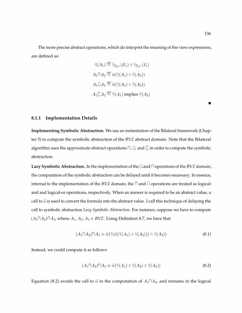
136
The more precise abstract operations, which do interpret the meaning of the view expressions,
are defined as:
γ(A1) def= γE2w (E1) ∧ γI2w (I1)
A1uA2def= α(γ(A1) ∧ γ(A2))
A1tA2def= α(γ(A1) ∨ γ(A2))
A1vA2def= γ(A1) implies γ(A2)
�
8.1.1 Implementation Details
Implementing Symbolic Abstraction. We use an instantiation of the Bilateral framework (Chap-
ter 5) to compute the symbolic abstraction of the BVI abstract domain. Note that the Bilateral
algorithm uses the approximate abstract operations u, t, and v in order to compute the symbolic
abstraction.
Lazy Symbolic Abstraction. In the implementation of the t and u operations of theBVI domain,
the computation of the symbolic abstraction can be delayed until it becomes necessary. In essence,
internal to the implementation of the BVI domain, the u and t operations are treated as logical-
and and logical-or operations, respectively. When an answer is required to be an abstract value, a
call to α is used to convert the formula into the abstract value. I call this technique of delaying the
call to symbolic abstraction Lazy Symbolic Abstraction. For instance, suppose we have to compute
(A1uA2)uA3, where A1, A2, A3 ∈ BVI. Using Definition 8.7, we have that
(A1uA2)uA3 ≡ α(γ(α(γ(A1) ∧ γ(A2))
)∧ γ(A3)
)(8.1)
Instead, we could compute it as follows:
(A1uA2)uA3 ≡ α(γ(A1) ∧ γ(A2) ∧ γ(A3)
)(8.2)
Equation (8.2) avoids the call to α in the computation of A1uA2, and remains in the logical
137
domain. The call to α is delayed until the end of the computation of the meets. There are two
advantages of delaying the call to α as shown in Equation (8.2):
• Precision: Equation (8.2) avoids going back to the (less precise) abstract domain, and stays
in the logical domain.
• Speed: Equation (8.2) has a single call to α.
This same approach of delaying the call to α applies to the implementation of t. In practice, we
perform an α operation that converts the internal formula representation into an abstract value
when either of the following conditions are met:
• The number of conjunctions and disjunctions in the formula exceed a fixed threshold k.
• The join operation is performed at a loop header, or, more generally, at a widening point
(Bourdoncle, 1993).
Heuristics for picking view expressions. When performing machine-code analysis, the choice
of view expressions determines the precision of the abstract domain. In practice, the view
expressions include memory accesses performed by the program. We also determine the branch
predicates occurring in the program, and add these as view expressions. The branch predicate
is computing by first performing symbolic execution of the basic block that ends in a branch
instruction, and then inspecting the expression for the program counter in the symbolic state.
Given a (Boolean) branch predicate b, we add the view expression ITE(b, 1232 , 0232), where
ITE is the if-then-else term. This enables the BVI abstract domain to behave similarly to a
Cartesian predicate-abstraction domain (Flanagan and Qadeer, 2002), in that the BVI is capable
of expressing conjunctions of predicates. However, the use the affine-equalities domain allows
the BVI domain to also express a logical-xor of predicates, hence, making the domain more
expressive than a Cartesian predicate-abstraction domain. This concept is illustrated in the next
example.

138
Example 8.8. Consider the view expressions t1 ≡ ITE(b1, 1232 , 0232), and t2 ≡ ITE(b2, 1232 , 0232),
and let T ≡ {t1, t2}.
a1 ≡ {t1 = 1, t2 = 0} ∈ BVI232 [T ] γ(a1) = b1 ∧ ¬b2
a2 ≡ {t1 + t2 = 2} ∈ BVI232 [T ] γ(a2) = b1 ∧ b2
a1 ≡ {t1 + t2 = 1} ∈ BVI232 [T ] γ(a3) = b1⊕ b2
�
Picking the right set of view expressions is an interesting and challenging research question
in itself. Exploring techniques based on, for example, counter-example guided abstraction
refinement (CEGAR) is left as future work. Section 9.4 describes an experimental evaluation of
the BVI abstract domain.
8.2 Related Work
Other work on identifying bit-vector-inequality invariants includes Brauer and King (2010,
2011) and Masdupuy (1992). Masdupuy (1992) proposed a relational abstract domain of interval
congruences on rationals. One limitation of his machinery is that the domain represents diagonal
grids of parallelepipeds, where the dimension of each parallelepiped equals the number of
variables tracked (say n). In our work, we can have any number of view-variables, which means
that the point-spaces represented can be constrained by more than n constraints.
Brauer and King employ bit-blasting to synthesize abstract transformers for the interval and
octagon (Miné, 2001) domains. One of their papers uses universal-quantifier elimination on
Boolean formulas (Brauer and King, 2010); the other avoids quantifier elimination (Brauer and
King, 2011). Compared with their work, we avoid the use of bit-blasting and work directly with
representations of sets of w-bit bit-vectors.
Chang and Leino (2005) developed a technique for extending the properties representable by
a given abstract domain from schemas over variables to schemas over terms. To orchestrate the
communication of information between domains, they designed the congruence-closure abstract
domain, which introduces variables to stand for subexpressions that are alien to a base domain; to

139
the base domain, these expressions are just variables. Their scheme for propagating information
between domains is mediated by the e-graph of the congruence-closure domain. In contrast,
our method can make use of symbolic abstraction to propagate information between domains.
Cousot et al. (2011b) have recently studied the iterated pairwise exchange of observations between
components as a way to compute an over-approximation of a reduced product.
Chen et al. (2008) devised a way to use the polyhedral domain (Cousot and Halbwachs, 1978)
to analyze programs that use floating-point computations. They use a linearization technique
developed by Miné (2004), which soundly abstracts the floating-point computations performed in
a program being analyzed into computations on reals. These values are then over-approximated
using a variant of the polyhedral domain in which two of the underlying primitives are replaced
by floating-point versions that use interval arithmetic with outward rounding to compute
answers in floating-point arithmetic that over-approximate the exact real counterparts. Both
of the replaced primitives can produce a floating-point overflow or the value NaN (Not a
Number). In these cases, a sound answer is created by discarding a constraint. By this means, it
is possible to use the floating-point polyhedral domain to analyze programs that use floating-
point computations.
8.3 Chapter Notes
Tushar Sharma helped with part of the implementation and experimental evaluation of the
BVI domain; I was responsible for idea behind of the BVI domain, and most of the design and
implementation of the domain.

140
Chapter 9
Symbolic Abstraction for
Machine-Code Verification
This chapter describes a model-checking algorithm for stripped machine-code, called MCVETO
(Machine-Code VErification TOol). The unique challenges and opportunities in verification
of stripped machine-code, as well as a comparison of MCVETO with previous machine-code
analysis tools, can be found in Chapter 2. In particular, MCVETO is able to detect and explore
“deviant behavior” in machine code. An example of such deviant behavior is when the program
over-writes the return address stored on the stack frame, as illustrated in Section 2.3. In MCVETO,
deviant behavior is reported as an acceptable-execution (AE) violation. Moreover, MCVETO is capable
of verifying (or detecting flaws in) self-modifying code (SMC). To the best of my knowledge,
MCVETO is the first model checker to handle SMC.
The specific problem addressed by MCVETO can be stated as follows: Given a stripped
machine-code program P , and a (bad) target state, find either
• an input to P that results in an AE violation,
• an input to P that causes the target state to be reached, or
• a proof that P performs only AEs, and the bad state cannot be reached during any AE.
141
The (bad) target state is usually specified as a particular value of the program counter (PC),
which we denote by target.
MCVETO works by starting with an initial coarse abstraction of the program’s state space.
The initial abstraction has only two abstract states, defined by the predicates “PC = target” and
“PC 6= target” . The abstraction is gradually refined during subsequent analysis steps. Thus, the
MCVETO algorithm can be viewed as computing the symbolic abstraction of a machine-code
program with respect to a particular graph-based abstract domain.
The contributions of this chapter can be summarized as follows:
1. I describe how MCVETO adapts directed proof generation (DPG) (Gulavani et al., 2006) for
model checking stripped machine code (Section 9.1).
2. I describe how MCVETO uses trace-based generalization to build and refine an abstraction of
the program’s state space entirely on-the-fly (Section 9.2.2). Trace-based generalization
enables MCVETO to handle instruction aliasing and SMC.
3. I describe how MCVETO uses speculative trace refinement to identify candidate invariants that
can speed up the convergence of DPG (Section 9.2.3).
4. I introduce a new approach to performing DPG on multi-procedure programs (Section 9.2.4).
5. I describe a language-independent algorithm to identify the aliasing condition relevant to
a property in a given state (Section 9.2.5).
Item 2 addresses execution details that are typically ignored (unsoundly) by source-code
analyzers. Items 2, 3, 4, and 5 are applicable to both source-code and machine-code analysis.
Section 9.3 describes the implementation details of MCVETO; Section 9.4 presents an experi-
mental evaluation of MCVETO; Section 9.5 presents related work.

142
n’ : � ∧ ¬�
k
n : �
m : �
k
n’’ : � ∧ �
I
⟹
I
m : �
♦ ♦
♦ ♦
Figure 9.1: The general refinement step across frontier (n, I,m). The presence of a witness isindicated by a “�” inside of a node.
9.1 Background on Directed Proof Generation (DPG)
Given a program P and a particular control location target in P , DPG returns either an input for
which execution leads to target or a proof that target is unreachable (or DPG does not terminate).
Two approximations of P ’s state space are maintained:
• A set T of concrete traces, obtained by runningP with specific inputs. T underapproximates
P ’s state space.
• A graph G, called the abstract graph, obtained from P via abstraction (and abstraction
refinement). G overapproximates P ’s state space.
Nodes in G are labeled with formulas; edges are labeled with program instructions or program
conditions. One node is the start node (where execution begins); another node is the target node
(the goal to reach). Information to relate the under- and overapproximations is also maintained:
a concrete state σ in a trace in T is called a witness for a node n in G if σ satisfies the formula that
labels n.
If G has no path from start to target, then DPG has proved that target is unreachable, and G
serves as the proof. Otherwise, DPG locates a frontier: a triple (n, I,m), where (n,m) is an edge
on a path from start to target such that n has a witness w but m does not, and I is the instruction
on (n,m). DPG either performs concrete execution (attempting to reach target) or refines G by
splitting nodes and removing certain edges (which may prove that target is unreachable). Which
action to perform is determined using the basic step from directed test generation (Godefroid
et al., 2005), which uses symbolic execution to try to find an input that allows execution to

143
cross frontier (n, I,m). Symbolic execution is performed over symbolic states, which have two
components: a path constraint, which represents a constraint on the input state, and a symbolic map,
which represents the current state in terms of input-state quantities. DPG performs symbolic
execution along the path taken during the concrete execution that produced witness w for n;
it then symbolically executes I , and conjoins to the path constraint the formula obtained by
evaluating m’s predicate ψ with respect to the symbolic map. It calls an SMT solver to determine
if the path constraint obtained in this way is satisfiable. If so, the result is a satisfying assignment
that is used to add a new execution trace to T . If not, DPG refines G by splitting node n into n′
and n′′, as shown in Figure 9.1.
Refinement changes G to represent some non-connectivity information: in particular, n′ is not
connected to m in the refined graph (see Figure 9.1). Let ψ be the formula that labels m, c be the
concrete witness of n, and Sn be the symbolic state obtained from the symbolic execution up
to n. DPG chooses a formula ρ, called the refinement predicate, and splits node n into n′ and n′′
to distinguish the cases when n is reached with a concrete state that satisfies ρ (n′′) and when
it is reached with a state that satisfies ¬ρ (n′). The predicate ρ is chosen such that (i) no state
that satisfies ¬ρ can lead to a state that satisfies ψ after the execution of I , and (ii) the symbolic
state Sn satisfies ¬ρ. Condition (i) ensures that the edge from n′ to m can be removed. Condition
(ii) prohibits extending the current path along I (forcing the DPG search to explore different
paths). It also ensures that c is a witness for n′ and not for n′′ (because c satisfies Sn)—and thus
the frontier during the next iteration must be different.
9.2 MCVETO
This section explains the methods used to achieve contributions 2–5. While MCVETO was de-
signed to provide sound DPG for machine code, a number of its novel features are also useful
for source-code DPG. Thus, to make the chapter more accessible, our running example is the
C++ program in Figure 9.2. It makes a non-deterministic choice between two blocks that each
call procedure adjust, which loops—decrementing x and incrementing y. Note that the affine

144
int main() {int x, y;if(*) {
x = 200;y = 300;adjust(x, y);
}else {
x = 300;y = 200;adjust(x, y);
}if (y != 500)
UNREACHABLE();return 0;
}
void adjust(int& x, int& y) {while(x > 0) {
x--;y++;
}}
F
while(x>0)
T
x = 200
y = 300
F
x--
y++
x = 300
y = 200
exit
adju
st(x,y) adju
st(
x,y)
ret
ret
if(*)
if (y≠500)
T
FT
F
x = 300
F
x = 300
(a) (b)
Figure 9.2: (a) A program with a non-deterministic branch; (b) the program’s ICFG.
relation x+ y = 500 holds at the two calls on adjust, the loop-head in adjust, and the branch
on y!=500.
9.2.1 Representing the Abstract Graph
The infinite abstract graph used in MCVETO is finitely represented as a nested word automaton
(NWA) (Alur and Madhusudan, 2009) and queried by symbolic operations.
Definition 9.1 (Alur and Madhusudan (2009)). A nested word (w, ) over alphabet Σ is an
ordinary word w ∈ Σ∗, together with a nesting relation of length |w|. is a collection of
edges (over the positions in w) that do not cross. A nesting relation of length l ≥ 0 is a subset of
{−∞, 1, 2, . . . , l} × {1, 2, . . . , l,+∞} such that
• Nesting edges only go forwards: if i j then i < j.
• No two edges share a position: for 1 ≤ i ≤ l, |{j | i j}| ≤ 1 and |{j | j i}| ≤ 1.
• Edges do not cross: if i j and i′ j′, then one cannot have i < i′ ≤ j < j′.
When i j holds, for 1 ≤ i ≤ l, i is called a call position; if i +∞, then i is a pending
call; otherwise i is a matched call, and the unique position j such that i j is called its return
145
successor. Similarly, when i j holds, for 1 ≤ j ≤ l, j is a return position; if −∞ j, then j is
a pending return, otherwise j is a matched return, and the unique position i such that i j is
called its call predecessor. A position 1 ≤ i ≤ l that is neither a call nor a return is an internal
position.
MatchedNW denotes the set of nested words that have no pending calls or returns. NWPrefix
denotes the set of nested words that have no pending returns.
A nested word automaton (NWA) A is a 5-tuple (Q,Σ, q0, δ, F ), where Q is a finite set of
states, Σ is a finite alphabet, q0 ∈ Q is the initial state, F ⊆ Q is a set of final states, and δ is a
transition relation. The transition relation δ consists of three components, (δc, δi, δr), where
• δi ⊆ Q× Σ×Q is the transition relation for internal positions.
• δc ⊆ Q× Σ×Q is the transition relation for call positions.
• δr ⊆ Q×Q× Σ×Q is the transition relation for return positions.
Starting from q0, an NWAA reads a nested word nw = (w, ) from left to right, and performs
transitions (possibly non-deterministically) according to the input symbol and . If A is in state
q when reading input symbol σ at position i in w, and i is an internal or call position, A makes a
transition to q′ using (q, σ, q′) ∈ δi or (q, σ, q′) ∈ δc, respectively. If i is a return position, let k be
the call predecessor of i, and qc be the state A was in just before the transition it made on the
kth symbol; A uses (q, qc, σ, q′) ∈ δr to make a transition to q′. If, after reading nw, A is in a state
q ∈ F , then A accepts nw. �
As discussed in Section 9.2.2 the key property of NWAs for abstraction refinement is that,
even though they represent matched call/return structure, they are closed under intersection
(Alur and Madhusudan, 2009). That is, given NWAs A1 and A2, one can construct an NWA A3
such that L(A3) = L(A1) ∩ L(A2).
In our NWAs, the alphabet consists of all possible machine-code instructions. In addition, we
annotate each state with a predicate. Operations on NWAs extend cleanly to accommodate the
semantics of predicates—e.g., the ∩ operation labels a product state 〈q1, q2〉with the conjunction
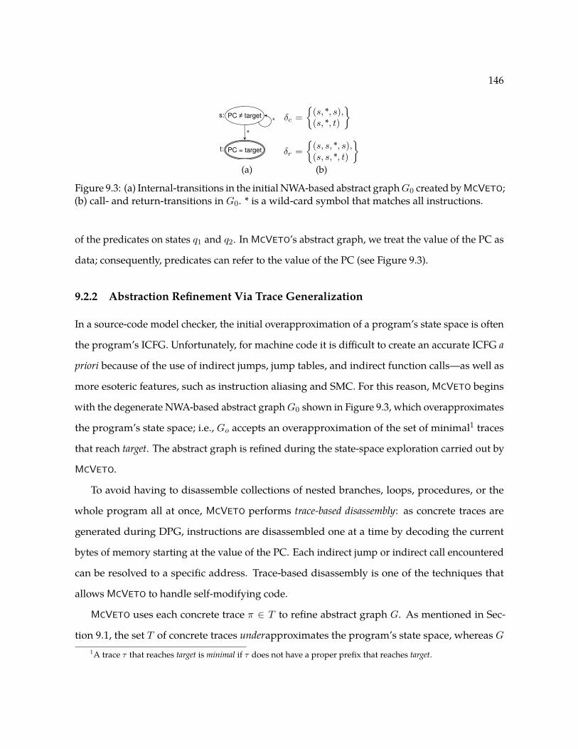
146
PC ≠ targets:
*
*
PC = targett:
δc ={
(s, *, s),(s, *, t)
}
δr ={
(s, s, *, s),(s, s, *, t)
}(a) (b)
Figure 9.3: (a) Internal-transitions in the initial NWA-based abstract graphG0 created by MCVETO;(b) call- and return-transitions in G0. * is a wild-card symbol that matches all instructions.
of the predicates on states q1 and q2. In MCVETO’s abstract graph, we treat the value of the PC as
data; consequently, predicates can refer to the value of the PC (see Figure 9.3).
9.2.2 Abstraction Refinement Via Trace Generalization
In a source-code model checker, the initial overapproximation of a program’s state space is often
the program’s ICFG. Unfortunately, for machine code it is difficult to create an accurate ICFG a
priori because of the use of indirect jumps, jump tables, and indirect function calls—as well as
more esoteric features, such as instruction aliasing and SMC. For this reason, MCVETO begins
with the degenerate NWA-based abstract graphG0 shown in Figure 9.3, which overapproximates
the program’s state space; i.e., Go accepts an overapproximation of the set of minimal1 traces
that reach target. The abstract graph is refined during the state-space exploration carried out by
MCVETO.
To avoid having to disassemble collections of nested branches, loops, procedures, or the
whole program all at once, MCVETO performs trace-based disassembly: as concrete traces are
generated during DPG, instructions are disassembled one at a time by decoding the current
bytes of memory starting at the value of the PC. Each indirect jump or indirect call encountered
can be resolved to a specific address. Trace-based disassembly is one of the techniques that
allows MCVETO to handle self-modifying code.
MCVETO uses each concrete trace π ∈ T to refine abstract graph G. As mentioned in Sec-
tion 9.1, the set T of concrete traces underapproximates the program’s state space, whereas G1A trace τ that reaches target is minimal if τ does not have a proper prefix that reaches target.

147
♦
F
while(x>0)
T
x = 200
y = 300
F
x--
y++
exit
adjust(x,y)
if(*)
if (y≠500)
T
TS
*
♦♦
♦
♦
♦
♦
♦
♦ ♦
♦
FT
ret
(a)
FT
F
x--
y++
x = 300
y = 200
adju
st(x
,y)
ret
T
FT
TS
*
while(x>0)
exitif(*)
if (y≠500)
♦♦
♦
♦
♦ ♦
♦
♦
♦
♦
♦
(b)
x = 300
while(x>0)
T
x = 200
y = 300
F
x--
y++
exitif(*)
if (y≠500)
T
TS
*♦♦
♦
♦
♦
♦
♦
♦ ♦
♦
♦
FTy = 200
adjust(x,y) a
dju
st(
x,y)
F
ret
ret
♦
♦
♦
(c)
Figure 9.4: (a) and (b) show two generalized traces, each of which reaches the end of the program.(c) shows the intersection of the two generalized traces. (“�” indicates that a node has a witness.)
represents an overapproximation of the state space. MCVETO repeatedly solves instances of the
following trace-generalization problem:Given a trace π, which is an underapproximation of the program, convert π into an NWA-based
abstract graph Gπ that is an overapproximation of the program.A trace π that does not reach target is represented by (i) a nested-word prefix (w, ) over
instructions (Definition 9.1), together with (ii) an array of PC values, PC[1..|w| + 1], where
PC[|w|+ 1] has the special value HALT if the trace terminated execution. Internal-steps, call-
steps, and return-steps are triples of the form 〈PC[i], w[i],PC[i+ 1]〉, 1 ≤ i < |w|, depending on
whether i is an internal-position, call-position, or return-position, respectively. We create Gπ
by “folding” π—grouping together all nodes with the same PC value, and augmenting it in a
way that overapproximates the portion of the program not explored by π (denoted by π/[PC]);
see Figures 9.4(a), 9.4(b), and 9.5. In particular, Gπ contains one accepting state, called TS (for
“target surrogate”). TS is an accepting state because it represents target, as well as all non-target
locations not visited by π.
We now have two overapproximations, the original abstract graph G and folded trace Gπ.
Abstract graphs are based on NWAs, and hence closed under intersection. Thus, by performing
G := G∩Gπ, information about the portion of the program explored by π is incorporated into G,
producing a third, improved overapproximation; see Figure 9.4(c). Equivalently, intersection elim-
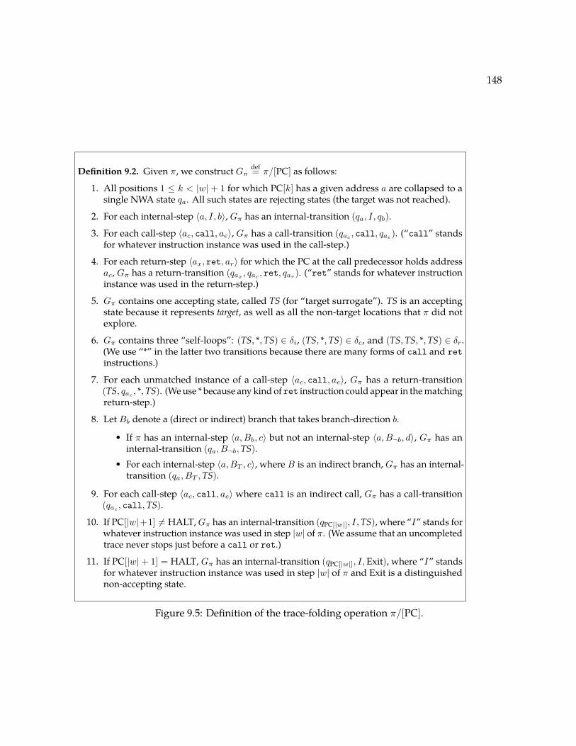
148
Definition 9.2. Given π, we construct Gπdef= π/[PC] as follows:
1. All positions 1 ≤ k < |w| + 1 for which PC[k] has a given address a are collapsed to asingle NWA state qa. All such states are rejecting states (the target was not reached).
2. For each internal-step 〈a, I, b〉, Gπ has an internal-transition (qa, I, qb).
3. For each call-step 〈ac, call, ae〉, Gπ has a call-transition (qac, call, qae
). (“call” standsfor whatever instruction instance was used in the call-step.)
4. For each return-step 〈ax, ret, ar〉 for which the PC at the call predecessor holds addressac, Gπ has a return-transition (qax
, qac, ret, qar
). (“ret” stands for whatever instructioninstance was used in the return-step.)
5. Gπ contains one accepting state, called TS (for “target surrogate”). TS is an acceptingstate because it represents target, as well as all the non-target locations that π did notexplore.
6. Gπ contains three “self-loops”: (TS, *,TS) ∈ δi, (TS, *,TS) ∈ δc, and (TS,TS, *,TS) ∈ δr.(We use “*” in the latter two transitions because there are many forms of call and retinstructions.)
7. For each unmatched instance of a call-step 〈ac, call, ae〉, Gπ has a return-transition(TS, qac
, *,TS). (We use * because any kind of ret instruction could appear in the matchingreturn-step.)
8. Let Bb denote a (direct or indirect) branch that takes branch-direction b.
• If π has an internal-step 〈a,Bb, c〉 but not an internal-step 〈a,B¬b, d〉, Gπ has aninternal-transition (qa, B¬b,TS).
• For each internal-step 〈a,BT , c〉, where B is an indirect branch, Gπ has an internal-transition (qa, BT ,TS).
9. For each call-step 〈ac, call, ae〉 where call is an indirect call, Gπ has a call-transition(qac
, call,TS).
10. If PC[|w|+1] 6= HALT,Gπ has an internal-transition (qPC[|w|], I,TS), where “I” stands forwhatever instruction instance was used in step |w| of π. (We assume that an uncompletedtrace never stops just before a call or ret.)
11. If PC[|w|+ 1] = HALT, Gπ has an internal-transition (qPC[|w|], I,Exit), where “I” standsfor whatever instruction instance was used in step |w| of π and Exit is a distinguishednon-accepting state.
Figure 9.5: Definition of the trace-folding operation π/[PC].

149
Algorithm 19: Basic MCVETO algorithm (including trace-based disassembly)1 π := nested-word prefix for an execution run on a random initial state2 T := {π}; Gπ := π/[PC]; G := (NWA from Figure 9.3) ∩ Gπ3 while true do4 if target has a witness in T then5 return “reachable”6 Find a path τ in G from start to target7 if no path exists then8 return “not reachable”9 Find a frontier (n, I,m) in G, where concrete state σ witnesses n
10 Perform symbolic execution of the instructions of the concrete trace that reaches σ, andthen of instruction I ; conjoin to the path constraint the formula obtained by evaluating m’spredicate ψ with respect to the symbolic map; let S be the path constraint so obtained
11 if S is feasible, with satisfying assignment A then12 π := nested-word prefix for an execution run on A13 T := T ∪ {π}; Gπ := π/[PC]; G := G ∩Gπ14 else15 Refine G along frontier (n, I,m) (see Figure 9.1)
inates the family of infeasible traces represented by the complement of Gπ; however, because we
already have Gπ in hand, no automaton-complementation operation is required—cf. (Heizmann
et al., 2010).
The issue of how one forms an NWPrefix from an instruction sequence—i.e., identifying the
nesting structure—is handled by a policy in the trace-recovery tool for classifying each position
as an internal-, call-, or return-position. Currently, for reasons discussed in Section 9.2.6, we
use the following policy: the position of any form of call instruction is a call-position; the
position of any form of ret instruction is a return-position. In essence, MCVETO uses call and
ret instructions to restrict the instruction sequences considered. If these match the program’s
actual instruction sequences, we obtain the benefits of the NWA-based approach—especially the
reuse of information among refinements of a given procedure. The basic MCVETO algorithm is
stated as Algorithm 19.

150
Trace Generalization for Self-Modifying Code
To perform trace generalization for self-modifying code, state names are now of the form qa,I ,
where a is an address and I is an instruction. Item 1 of the trace folding operation (Figure 9.5) is
changed to
• All positions 1 ≤ k < |w|+ 1 for which (i) PC[k] has a given address a, and (ii) w[k] has a
given instruction I are collapsed to a single NWA state qa,I . All such states are rejecting
states (the target was not reached).
Internal-, call-, and return-steps are now quadruples, 〈PC[i], w[i],PC[i+ 1], w[i+ 1]〉 depending
on whether i, for 1 ≤ i < |w|, is an internal-, call-, or return-position, respectively. Other items
are changed accordingly to account for instructions in state names. In addition, items 8–10 are
replaced by
• For each position i, 1 ≤ i < |w|+ 1, Gπ contains
– an internal-transition (qPC[i],w[i], ∗,TS)
– a call-transition (qPC[i],w[i], ∗,TS)
– a return-transition (qPC[i],w[i], qPC[j],w[j], ∗,TS), where 1 ≤ j < i and w[j] is the un-
matched call with largest index in w[1..i− 1].
9.2.3 Speculative Trace Refinement
Motivated by the observation that DPG is able to avoid exhaustive loop unrolling if it discovers
the right loop invariant, we developed mechanisms to discover candidate invariants from a folded
trace, which are then incorporated into the abstract graph via NWA intersection. Although they
are only candidate invariants, they are introduced into the abstract graph in the hope that they are
invariants for the full program. The basic idea is to apply dataflow analysis to a graph obtained
from the folded traceGπ. The recovery of invariants fromGπ is similar in spirit to the computation
of invariants from traces in Daikon (Ernst et al., 2007), but in MCVETO they are computed ex post

151
facto by dataflow analysis on the folded trace. While any kind of dataflow analysis could be used
in this fashion, MCVETO currently uses the BVI abstract domain (Chapter 8). Specifically, the
candidate invariant ψ at program point p is
ψ ≡ γ(⊔{
β(S)∣∣S is a concrete state at p}
)
The candidate invariants are used to create predicates for the nodes of Gπ. Because an
analysis may not account for the full effects of indirect memory references on the inferred
variables, to incorporate a discovered candidate invariant ϕ for node n into Gπ safely, we split n
on ϕ and ¬ϕ. Again we have two overapproximations: Gπ, from the folded trace, augmented
with the candidate invariants, and the original abstract graph G. To incorporate the candidate
invariants into G, we perform G := G ∩Gπ; the ∩ operation labels a product state 〈q1, q2〉with
the conjunction of the predicates on states q1 of G and q2 of Gπ.
Figure 9.6 shows how the candidate affine relation ϕ ≡ x+ y = 500 would be introduced at
the loop-head of adjust in the generalized traces from Figures 9.4(a) and 9.4(b). (Relation ϕ does,
in fact, hold for the portions of the state space explored by Figures 9.4(a) and 9.4(b).) With this
enhancement, subsequent steps of DPG will be able to show that the dotted loop-heads (labeled
with ¬ϕ) can never be reached from start. In addition, the predicate ϕ on the solid loop-heads
enables DPG to avoid exhaustive loop unrolling to show that the true branch of y!=500 can never
be taken.
9.2.4 Symbolic Methods for Interprocedural DPG
In other DPG systems (Gulavani et al., 2006; Beckman et al., 2008; Godefroid et al., 2010), in-
terprocedural DPG is performed by invoking intraprocedural DPG as a subroutine. In contrast,
MCVETO analyzes a representation of the entire program (refined on-the-fly), which allows it
to reuse all information from previous refinement steps. For instance, in the program shown
in Figure 9.7(a), procedure lotsaBaz makes several calls to baz. By invoking analysis once for
each call site on baz, a tool such as DASH has to re-learn that y is set to 0. In contrast, MCVETO

152
FT
x = 200
y = 300
exit
adju
st(x,y)
ret
if(*)
if (y≠500)
TS
*
♦♦
♦
♦
♦
♦
♦
FT
F
x--
y++T
while(x>0)♦
♦ ♦
♦φ ¬φwhile(x>0)
F
T
y++
ret
adjust(x,y)
FT
F
x--
y++
x = 300
y = 200
adju
st(x
,y)
ret
T
FT
TS
*
while(x>0)
exitif(*)
if (y≠500)
♦♦
♦
♦
♦ ♦
♦
♦
♦
♦
♦
φ ¬φwhile(x>0)
F
T
y++
ret
adju
st(x,y)
(a) (b)
Figure 9.6: Figures 9.4(a) and 9.4(b) with the loop-head in adjust split with respect to thecandidate invariant ϕ def= x+ y = 500.
int y;void baz(){
y=0;y++;y--;
}
void lotsaBaz(int a){y=0;if(a>0) baz();if(a>1) baz();if(a>2) baz();if(a>3) baz();if(y!=0)
ERR: return;}
int bar1() {int i,r = 0;for(i=0;i<100;i++){
complicated(); r++;}return r;
}
int bar2(){ return 10; }
void foo(int x){int y;if(x == 0) y = bar2();else y = bar1();if(y == 10)
ERR: return;}
(a) (b)
Figure 9.7: Programs that illustrate the benefit of using a conceptually infinite abstract graph.
only needs to learn this once and gets automatic reuse at all call sites. Note that such reuse
is achieved in a different way in SMASH (Godefroid et al., 2010), which makes use of explicit
procedure summaries. However, because the split between local and global variables is not
known when analyzing machine code, it is not clear to us how MCVETO could generate such
explicit summaries.
Furthermore, SMASH is still restricted to invoking intraprocedural analysis as a subroutine,
whereas MCVETO is not limited to considering frontiers in just a single procedure: at each stage,
it is free to choose a frontier in any procedure. To see why such freedom can be important,
consider the source-code example in Figure 9.7(b) (where target is ERR). DASH might proceed as
follows. The initial test uses [x 7→ 42], which goes through bar1, but does not reach target. After

153
a few iterations, the frontier is the call to bar1, at which point DASH is invoked on bar1 to prove
that the return value is not 10. The subproof takes a long time because of the complicated loop
in bar1. In essence, DASH gets stuck in bar1 without recourse to an easier way to reach target.
MCVETO can make the same choices, and would start to prove the same property for the return
value of bar1. However, refinements inside of bar1 cause the abstract graph to grow, and at
some point, if the policy is to pick a frontier closest to target, the frontier switches to one in main
that is closer to target—in particular, the true branch of the if-condition x==0. MCVETO will be
able to extend that frontier by running a test with [x 7→ 0], which will go through bar2 and reach
target. The challenge that we face to support such flexibility is how to select the frontier while
accounting for paths that reflect the nesting structure of calls and returns. As discussed below,
by doing computations via automata, transducers, and pushdown systems, MCVETO can find
the set of all frontiers, as well as identify the k closest frontiers.
Symbolic Methods to Find All Frontiers and Closest Frontiers
Definition 9.3. A configuration u of an NWA A is a sequence of states; that is, u ∈ Q∗. The
transition relation δ of A defines a transition relation δ⇒ on configurations of A as follows:
• if (q, σ, q′) ∈ δi, then qu δ⇒ q′u for all u ∈ Q∗
• if (qc, σ, qe) ∈ δc, then qcuδ⇒ qeqcu for all u ∈ Q∗
• if (qx, qc, σ, qr) ∈ δr, then qxqcuδ⇒ qru for all u ∈ Q∗ �
We often work with abstractions of NWAs in which alphabet symbols are dropped: ⇒def=⋃σ∈Σ
δ⇒. Let ⇒∗ denote the reflexive transitive closure of ⇒. For a set of configurations C,
pre∗(C) def= {c′ | ∃c ∈ C : c′ ⇒∗ c} and post∗(C) def= {c′ | ∃c ∈ C : c ⇒∗ c′}—i.e., backward and
forward reachability, respectively, with respect to transition relation⇒. When C is a regular
language of configurations, automata for the configuration languages pre∗(C) and post∗(C)
can be computed in polynomial time (Driscoll et al., 2012). Note that the check on line 6 of
Algorithm 19 can be performed by testing whether start ∈ pre∗(target).
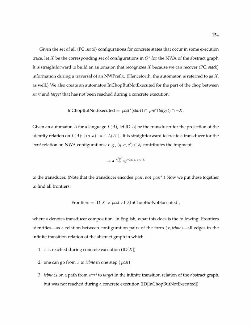
154
Given the set of all 〈PC, stack〉 configurations for concrete states that occur in some execution
trace, let X be the corresponding set of configurations in Q∗ for the NWA of the abstract graph.
It is straightforward to build an automaton that recognizes X because we can recover 〈PC, stack〉
information during a traversal of an NWPrefix. (Henceforth, the automaton is referred to as X ,
as well.) We also create an automaton InChopButNotExecuted for the part of the chop between
start and target that has not been reached during a concrete execution:
InChopButNotExecuted = post∗(start) ∩ pre∗(target) ∩ ¬X.
Given an automaton A for a language L(A), let ID[A] be the transducer for the projection of the
identity relation on L(A): {(a, a) | a ∈ L(A)}. It is straightforward to create a transducer for the
post relation on NWA configurations: e.g., (q, σ, q′) ∈ δi contributes the fragment
→ • q/q′→ } q/q, q ∈ Σ
to the transducer. (Note that the transducer encodes post, not post∗.) Now we put these together
to find all frontiers:
Frontiers = ID[X] ◦ post ◦ ID[InChopButNotExecuted],
where ◦ denotes transducer composition. In English, what this does is the following: Frontiers
identifies—as a relation between configuration pairs of the form (x, icbne)—all edges in the
infinite transition relation of the abstract graph in which
1. x is reached during concrete execution (ID[X])
2. one can go from x to icbne in one step ( post)
3. icbne is on a path from start to target in the infinite transition relation of the abstract graph,
but was not reached during a concrete execution (ID[InChopButNotExecuted])

155
The composition with the two projection functions, “ID[X]◦. . .” and “. . .◦ID[InChopButNotExecuted]”,
serves to specialize post to just the edges in the infinite transition relation of the abstract graph
that run between a configuration in X and a configuration in InChopButNotExecuted.
We can obtain “closest frontiers” by using weighted NWAs (Driscoll et al., 2012) and adding
shortest-distance weights to either pre∗(target) (to obtain frontiers that are closest to target) or to
post∗(start) (to obtain frontiers that are closest to start), and then carrying the weights through
the transducer-composition operations.
9.2.5 A Language-Independent Approach to Aliasing Relevant to a Property
This section describes how MCVETO identifies—in a language-independent way suitable for use
with machine code—the aliasing condition relevant to a property in a given state. Lim et al. (2009)
showed how to generate a Pre primitive for machine code; however, repeated application of Pre
causes refinement predicates to explode. We now present a language-independent algorithm
for obtaining an aliasing condition α that is suitable for use in machine-code analysis. From α,
one immediately obtains Preα. There are two challenges to defining an appropriate notion of
aliasing condition for use with machine code: (i) int-valued and address-valued quantities are
indistinguishable at runtime, and (ii) arithmetic on addresses is used extensively.
Suppose that the frontier is (n, I,m), ψ is the formula on m, and Sn is the symbolic state
obtained via symbolic execution of a concrete trace that reaches n. For source code, Beckman
et al. (2008) identify aliasing condition α by looking at the relationship, in Sn, between the
addresses written to by I and the ones used in ψ. However, their algorithm for computing α is
language-dependent: their algorithm has the semantics of C implicitly encoded in its search for
“the addresses written to by I”. In contrast, as explained below, we developed an alternative,
language-independent approach, both to identifying α and computing Preα. Further details on
this particular problem can be found in Thakur et al. (2010).
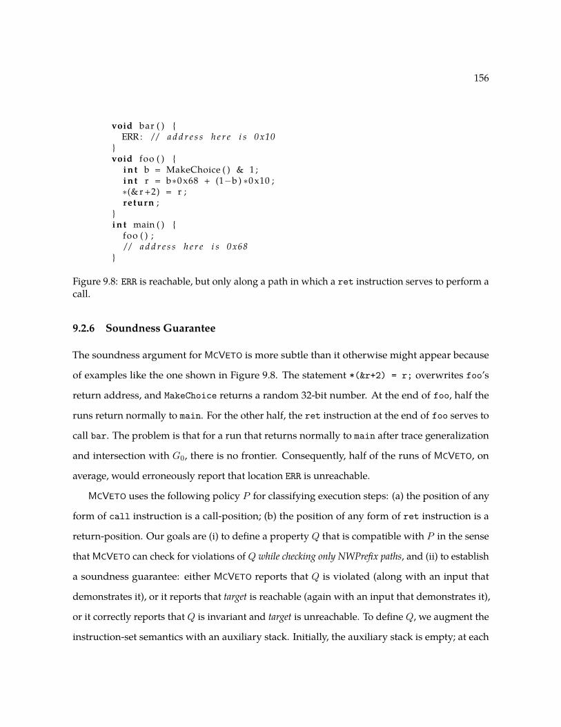
156
void bar ( ) {ERR : / / a d d r e s s h e r e i s 0x10
}void foo ( ) {
i n t b = MakeChoice ( ) & 1 ;i n t r = b∗0 x68 + (1−b ) ∗0 x10 ;∗(& r +2) = r ;return ;
}i n t main ( ) {
foo ( ) ;/ / a d d r e s s h e r e i s 0x68
}
Figure 9.8: ERR is reachable, but only along a path in which a ret instruction serves to perform acall.
9.2.6 Soundness Guarantee
The soundness argument for MCVETO is more subtle than it otherwise might appear because
of examples like the one shown in Figure 9.8. The statement *(&r+2) = r; overwrites foo’s
return address, and MakeChoice returns a random 32-bit number. At the end of foo, half the
runs return normally to main. For the other half, the ret instruction at the end of foo serves to
call bar. The problem is that for a run that returns normally to main after trace generalization
and intersection with G0, there is no frontier. Consequently, half of the runs of MCVETO, on
average, would erroneously report that location ERR is unreachable.
MCVETO uses the following policy P for classifying execution steps: (a) the position of any
form of call instruction is a call-position; (b) the position of any form of ret instruction is a
return-position. Our goals are (i) to define a property Q that is compatible with P in the sense
that MCVETO can check for violations of Q while checking only NWPrefix paths, and (ii) to establish
a soundness guarantee: either MCVETO reports that Q is violated (along with an input that
demonstrates it), or it reports that target is reachable (again with an input that demonstrates it),
or it correctly reports that Q is invariant and target is unreachable. To define Q, we augment the
instruction-set semantics with an auxiliary stack. Initially, the auxiliary stack is empty; at each
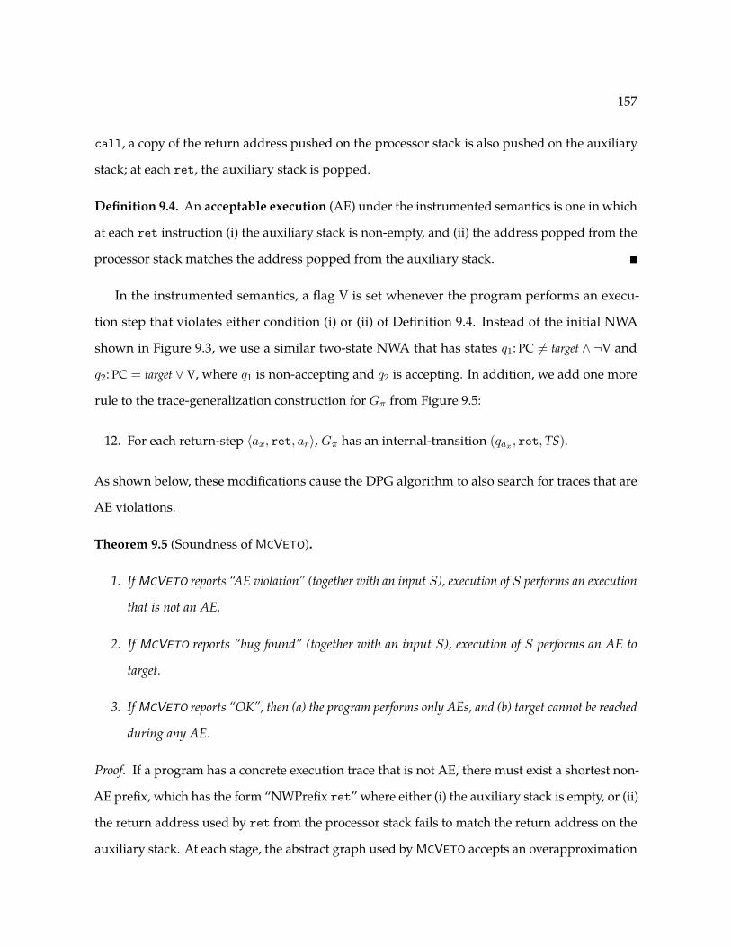
157
call, a copy of the return address pushed on the processor stack is also pushed on the auxiliary
stack; at each ret, the auxiliary stack is popped.
Definition 9.4. An acceptable execution (AE) under the instrumented semantics is one in which
at each ret instruction (i) the auxiliary stack is non-empty, and (ii) the address popped from the
processor stack matches the address popped from the auxiliary stack. �
In the instrumented semantics, a flag V is set whenever the program performs an execu-
tion step that violates either condition (i) or (ii) of Definition 9.4. Instead of the initial NWA
shown in Figure 9.3, we use a similar two-state NWA that has states q1: PC 6= target ∧ ¬V and
q2: PC = target ∨ V, where q1 is non-accepting and q2 is accepting. In addition, we add one more
rule to the trace-generalization construction for Gπ from Figure 9.5:
12. For each return-step 〈ax, ret, ar〉, Gπ has an internal-transition (qax , ret,TS).
As shown below, these modifications cause the DPG algorithm to also search for traces that are
AE violations.
Theorem 9.5 (Soundness of MCVETO).
1. If MCVETO reports “AE violation” (together with an input S), execution of S performs an execution
that is not an AE.
2. If MCVETO reports “bug found” (together with an input S), execution of S performs an AE to
target.
3. If MCVETO reports “OK”, then (a) the program performs only AEs, and (b) target cannot be reached
during any AE.
Proof. If a program has a concrete execution trace that is not AE, there must exist a shortest non-
AE prefix, which has the form “NWPrefix ret” where either (i) the auxiliary stack is empty, or (ii)
the return address used by ret from the processor stack fails to match the return address on the
auxiliary stack. At each stage, the abstract graph used by MCVETO accepts an overapproximation

158
of the program’s shortest non-AE execution-trace prefixes. This is true of the initial graph G0
because internal transitions have wild-card symbols. Moreover, each folded trace Gπ = π/[PC]
accepts traces of the form “NWPrefix ret” due to the addition of internal transitions to TS for
each ret instruction (item 12 above). NWA intersection of two sound overapproximations leads
to a refined sound overapproximation. Therefore, when MCVETO has shown that no accepting
state is reachable, it has also proved that the program has no AE violations.
For an example such as Figure 9.8, MCVETO reports “AE violation”.
In cases when MCVETO reports “AE violation”, it can indicate a stack-smashing attack. If
one wishes to find out more information when there is an AE violation, one can run a purely
intraprocedural version of MCVETO that does not give special treatment to call and ret instruc-
tions. This approach is potentially more expensive than running the interprocedural version of
MCVETO, but it can find out additional information about executions that are not AE.
9.3 Implementation
The MCVETO implementation incorporates all of the techniques described in Section 9.2. The
implementation uses only language-independent techniques; consequently, MCVETO can be easily
retargeted to different languages. The main components of MCVETO are language-independent
in two different dimensions:
1. The MCVETO DPG driver is structured so that one only needs to provide implementations
of primitives for concrete and symbolic execution of a language’s constructs, plus a handful
of other primitives (e.g., Preα). Consequently, this component can be used for both source-
level languages and machine-code languages.
2. For machine-code languages, I used two tools that generate the required implementations of
the primitives for concrete and symbolic execution from descriptions of the syntax and con-
crete operational semantics of an instruction set. The abstract syntax and concrete semantics
are specified using TSL (Lim and Reps, 2008). Translation of binary-encoded instructions

159
to abstract syntax trees is specified using a tool called ISAL (Instruction Set Architecture
Language).2 The relationship between ISAL and TSL is similar to the relationship between
Flex and Bison—i.e., a Flex-generated lexer passes tokens to a Bison-generated parser.
In our case, the TSL-defined abstract syntax serves as the formalism for communicating
values—namely, instructions’ abstract syntax trees—between the two tools.
To perform symbolic queries on the conceptually-infinite abstract graph Section 9.2.4), the
implementation uses OpenFst (Allauzen et al., 2007) (for transducers) and OpenNWA (Driscoll
et al., 2012) (for NWAs).
9.4 Experimental Evaluation
The experiments in this section were designed to answer the following questions:
1. How effective is the BVI abstract domain (Chapter 8) for verifying machine code?
2. How effective is MCVETO in verifying machine code?
3. How does speculative trace refinement (Section 9.2.3) impact the performance of MCVETO?
We used benchmarks taken from Gulavani et al. (2006). The examples are small, but challenging.
Our experiments (see Table 9.1) were run on a single core of a single-processor quad-core 3.0
GHz Xeon computer running Windows 7, configured so that a user process has 4 GB of memory.
The benchmarks were compiled using Visual Studio 2010, and the executables were analyzed
(without using symbol-table information). Out of the 16 benchmarks used, the target was
reachable in 4, and the target PC was unreachable in 12; in Table 9.1, [ ] means the target PC is
reachable, [9] means the target PC is unreachable.
Analysis based on BVI abstract domain was able to prove that the target was unreachable
for 8 out of the 12 unreachable benchmarks. An analysis based only on the affine-equality E232
2ISAL also handles other kinds of concrete syntactic issues, including (a) encoding (abstract syntax trees to binary-encoded instructions), (b) parsing assembly (assembly code to abstract syntax trees), and (c) assembly pretty-printing(abstract syntax trees to assembly code).
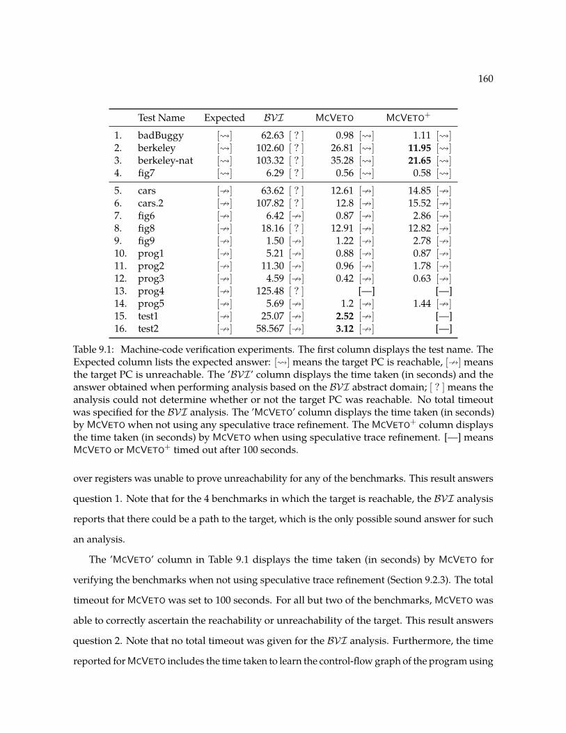
160
Test Name Expected BVI MCVETO MCVETO+
1. badBuggy [ ] 62.63 [ ? ] 0.98 [ ] 1.11 [ ]2. berkeley [ ] 102.60 [ ? ] 26.81 [ ] 11.95 [ ]3. berkeley-nat [ ] 103.32 [ ? ] 35.28 [ ] 21.65 [ ]4. fig7 [ ] 6.29 [ ? ] 0.56 [ ] 0.58 [ ]
5. cars [9] 63.62 [ ? ] 12.61 [9] 14.85 [9]6. cars.2 [9] 107.82 [ ? ] 12.8 [9] 15.52 [9]7. fig6 [9] 6.42 [9] 0.87 [9] 2.86 [9]8. fig8 [9] 18.16 [ ? ] 12.91 [9] 12.82 [9]9. fig9 [9] 1.50 [9] 1.22 [9] 2.78 [9]10. prog1 [9] 5.21 [9] 0.88 [9] 0.87 [9]11. prog2 [9] 11.30 [9] 0.96 [9] 1.78 [9]12. prog3 [9] 4.59 [9] 0.42 [9] 0.63 [9]13. prog4 [9] 125.48 [ ? ] [—] [—]14. prog5 [9] 5.69 [9] 1.2 [9] 1.44 [9]15. test1 [9] 25.07 [9] 2.52 [9] [—]16. test2 [9] 58.567 [9] 3.12 [9] [—]
Table 9.1: Machine-code verification experiments. The first column displays the test name. TheExpected column lists the expected answer: [ ] means the target PC is reachable, [9] meansthe target PC is unreachable. The ’BVI’ column displays the time taken (in seconds) and theanswer obtained when performing analysis based on the BVI abstract domain; [ ? ] means theanalysis could not determine whether or not the target PC was reachable. No total timeoutwas specified for the BVI analysis. The ’MCVETO’ column displays the time taken (in seconds)by MCVETO when not using any speculative trace refinement. The MCVETO+ column displaysthe time taken (in seconds) by MCVETO when using speculative trace refinement. [—] meansMCVETO or MCVETO+ timed out after 100 seconds.
over registers was unable to prove unreachability for any of the benchmarks. This result answers
question 1. Note that for the 4 benchmarks in which the target is reachable, the BVI analysis
reports that there could be a path to the target, which is the only possible sound answer for such
an analysis.
The ’MCVETO’ column in Table 9.1 displays the time taken (in seconds) by MCVETO for
verifying the benchmarks when not using speculative trace refinement (Section 9.2.3). The total
timeout for MCVETO was set to 100 seconds. For all but two of the benchmarks, MCVETO was
able to correctly ascertain the reachability or unreachability of the target. This result answers
question 2. Note that no total timeout was given for the BVI analysis. Furthermore, the time
reported for MCVETO includes the time taken to learn the control-flow graph of the program using

161
trace generalization (Section 9.2.2); on the other hand, the BVI analysis uses CodeSurfer/x86
(Balakrishnan et al., 2005) to construct the control-flow graph.
In Table 9.1, MCVETO+ represents the MCVETO algorithm when using speculative trace
refinement. MCVETO+ performs better than MCVETO for two of the reachable benchmarks, while
it performs worse for two unreachable benchmarks, as highlighted in Table 9.1. This experiment
answers question 3.
9.5 Related Work
Machine-Code Analyzers Targeted at Finding Vulnerabilities. A substantial amount of work
exists on techniques to detect security vulnerabilities by analyzing source code for a variety
of languages (Wagner et al., 2000; Livshits and Lam, 2005; Xie and Aiken, 2006). Less work
exists on vulnerability detection for machine code. Kruegel et al. (2005) developed a system
for automating mimicry attacks; it uses symbolic execution to discover attacks that can give up
and regain execution control by modifying the contents of the data, heap, or stack so that the
application is forced to return control to injected attack code at some point after the execution
of a system call. Cova et al. (2006) used that platform to detect security vulnerabilities in x86
executables via symbolic execution.
Prior work exists on directed test generation for machine code (Godefroid et al., 2008; Brumley
et al., 2008). Directed test generation combines concrete execution and symbolic execution to find
inputs that increase test coverage. An SMT solver is used to obtain inputs that force previously
unexplored branch directions to be taken. In contrast, MCVETO implements directed proof
generation. Unlike directed-test-generation tools, MCVETO is goal-directed, and works by trying
to refute the claim “no path exists that connects program entry to a given goal state”.
Machine-Code Model Checkers. The SYNERGY model checker can be used to verify safety
properties of an x86 executable compiled from a “single-procedure C program with only [int-
valued] variables” (Gulavani et al., 2006) (i.e., no pointers). It uses debugging information to
obtain information about variables and types, and uses Vulcan (Srivastava et al., 2001) to obtain

162
a CFG. It uses integer arithmetic—not bit-vector arithmetic—in its solver. In contrast, MCVETO
addresses the challenges of checking properties of stripped executables.
AIR (“Assembly Iterative Refinement”) (Chaki and Ivers, 2009) is a model checker for PowerPC.
AIR decompiles an assembly program to C, and then checks if the resulting C program satisfies
the desired property by applying COPPER (Chaki et al., 2004), a predicate-abstraction-based
model checker for C source code. They state that the choice of COPPER is not essential, and that
any other C model checker, such as SLAM (Ball and Rajamani, 2001) or BLAST (Henzinger et al.,
2002) would be satisfactory. However, the C programs that result from their translation step use
pointer arithmetic and pointer dereferencing, whereas many C model checkers, including SLAM
and BLAST, make unsound assumptions about pointer arithmetic.
[MC]SQUARE (Schlich, 2008) is a model checker for microcontroller assembly code. It uses
explicit-state model-checking techniques (combined with a degree of abstraction) to check CTL
properties.
Self-Modifying Code. The work on MCVETO addresses a problem that has been almost entirely
ignored by the PL research community. There is a paper on SMC by Gerth (1991), and a recent
paper by Cai et al. (2007). However, both of the papers concern proof systems for reasoning
about SMC. In contrast, MCVETO can verify (or detect flaws in) SMC automatically.
As far as I know, MCVETO is the first model checker to address verifying (or detecting flaws
in) SMC.
Trace Generalization. The trace-generalization technique of Section 9.2.2 has both similarities
to and differences from the path programs of Beyer et al. (2007) and the trace-refinement technique
of Heizmann et al. (2010). All three techniques refine an overapproximation to eliminate families
of infeasible concrete traces. However, trace generalization obtains the desired outcome in a
substantially different way. Beyer et al. analyze refuted abstract traces to obtain new predicates
to refine the predicate abstraction in use. The subsequent refinement step requires possibly
expensive calls on an SMT solver to compute new abstract transformers. Heizmann et al. adopt
a language-theoretic viewpoint: once a refutation automaton is constructed—which involves

163
calling an SMT solver and an interpolant generator—refinement is performed by automaton com-
plementation followed by automaton intersection. In contrast, our generalized traces are created
by generalizing a feasible concrete trace to create directly a representation that overapproximates the
set of minimal traces that reach target. Consequently, refinement by trace generalization involves
no calls on an SMT solver, and avoids the potentially expensive step of automaton complementation.
9.6 Chapter Notes
The design and implementation of MCVETO was based on that of the MCDASH tool (Lal et al.,
2009). In particular, both tools use directed proof generation (Section 9.1) and a language-
independent algorithm to identify aliasing relevant to a property (Section 9.2.5). However, the
techniques for trace generalization (Section 9.2.2), speculative trace refinement (Section 9.2.3),
interprocedural DPG (Section 9.2.4), and finding acceptable-execution violations (Section 9.2.6)
are not found in MCDASH.

164
Chapter 10
A Distributed SAT Solver
Groups do not need to be dominated by exceptionally intelligent people
in order to be smart. Even if most of the people within a group are not
especially well-informed or rational, it can still reach a collectively wise
decision. This is a good thing, since human beings are not perfectly
designed decision makers. [. . .] Yet despite all these limitations, when
our imperfect judgments are aggregated in the right way, our collective
intelligence if often excellent.— James Surowiecki, The Wisdom of Crowds
In this chapter, I describe a new distributed SAT solver, called DiSSolve, which uses a new
proof rule that combines concepts from Stålmarck’s method with those found in modern SAT
solvers.
A modern sequential SAT solver usually implements same variant of the Davis, Putnam,
Logemann, and Loveland (DPLL) procedure (Davis et al., 1962). A DPLL-based SAT solver
performs a backtrack search over the set of assignments to literals. When a modern solver
reaches a conflict during the search, it generates a conflict clause (or learned clause) (Marques
Silva and Sakallah, 1996; Moskewicz et al., 2001). This learned clause enables the solver to prune
the search space. This technique for “learning from failure” is called Conflict-Driven Clause
Learning (CDCL). More information regarding DPLL/CDCL solvers can be found in Darwiche
and Pipatsrisawat (2009); Marques-Silva et al. (2009).

165
A modern parallel SAT solver falls into the following two categories:
• The divide-and-conquer approach incrementally divides the search space into subspaces,
which are then allocated to a DPLL/CDCL solver (Chrabakh and Wolski, 2003; Chu et al.,
2008). Care has to be taken to ensure load balancing when performing the division of the
search space.
• The Parallel Portfolio approach exploits the complementarity of different sequential DPLL/CDCL
strategies to let them compete and cooperate on the same formula (Hamadi et al., 2009b).
Though load balancing is not an issue in this approach, care has to be taken to craft the
individual strategies.
The DiSSolve algorithm (Section 10.1.1) presented in this chapter can be seen as combining
concepts from Stålmarck’s method and modern DPLL/CDCL solvers:
1. DiSSolve partitions the search space using k variables in the same fashion that the Dilemma
Rule partitions the search space in Stålmarck’s method.
2. Each of the 2k branches can be solved concurrently with the help of a sequential DPLL/CDCL
solver, similar to what is done in the divide-and-conquer approach discussed above.
3. The DPLL/CDCL solver assigned to a branch is allotted a finite amount of time, after
which the DPLL/CDCL solver returns a set of learned clauses. Such a branch-and-merge
approach does not have to as careful about load balancing, unlike the divide-and-conquer
approach.
4. DiSSolve performs a union of the information from all the branches, instead of an inter-
section as done in Stålmarck’s method. Performing a union of clauses is more effective
at pruning the search space compared to computing an intersection: with intersection
only common information learned by every process can be used to prune the search space,
while with union, all of the information learned by each process can be used to prune the
search space. In abstract-interpretation terms, DiSSolve combines the information from

166
the branches using a meet (u), while the Dilemma Rule in Stålmarck’s method combines
the information using a join (t).
The DiSSolve implementation (Section 10.1.2) also makes use of techniques already imple-
mented in modern DPLL/CDCL solvers, such as variable branching heuristics.
The contributions of this chapter can be summarized as follows:
• I describe, DiSSolve, a new SAT solver that combines the Dilemma rule in Stålmarck’s
method with clause-learning techniques from DPLL/CDCL solvers (Section 10.1).
• I evaluate the performance of DiSSolve when deployed on a multi-core machine and on
the cloud (Section 10.2).
• I present a natural extension of the DiSSolve algorithm from SAT to SMT, and describe
the DiSSolve algorithm as an SMA solver (Section 10.3).
Section 10.4 presents related work.
10.1 The DiSSolve Algorithm
This section explains the algorithm used in DiSSolve. Section 10.1.1 explains the basic algo-
rithm and skips over some of the details of the algorithm. These algorithm details are filled in
Section 10.1.2. Thus, Section 10.1.1 can be viewed as describing the algorithm mechanism, and
Section 10.1.2 describing the algorithm policy.
10.1.1 Basic Algorithm
Algorithm 20 shows the basic DiSSolve algorithm for deciding the satisfiability of a propositional-
logic formula ϕ. C is a set of clauses, which is initialized to the empty set (line 1). Recall that
a clause c is a disjunction of literals. I use ε to represent an empty clause, whose meaning is to
be interpreted as false. The meaning of a set of clauses C = {c1, c2, . . . , cn} is: JCK def=∧
1≤i≤n ci.
The meaning of the empty set of clauses ∅ is true.

167
Algorithm 20: DiSSolve(ϕ)1 C ← ∅2 for j ∈ {0, 1, 2, . . .} do3 Vj ← SplittingVariables(j)4 tj ← TimeBudget(j)5 (ansj , C)← DiSSolveSplit(ϕ,C, Vj , tj)6 if ansj is sat or ansj is unsat then7 return ansj
Algorithm 21: DissolveSplit(ϕ,C, V, t)1 k ← |V |2 {a0, a1, . . . , a2k−1} ← DilemmaAssumptions(V )3 for i ∈ {0, 1, . . . , 2k − 1} do4 (ansi, Ci)← Deduce(ϕ,C, ai, t)5 if ansi is sat then6 return (sat, ∅)7 if all ansi are unsat then8 return (unsat, {ε})9 C ′ ← UnionClauses(C,C0, C1, C2 . . . , C2k−1)
10 return (unknown, C ′)
In the loop from lines 2–7, DiSSolve repeatedly calls DiSSolveSplit (Algorithm 21). The loop
invariant is ϕ⇒C. Vj is a set of variables to be used in iteration j, which are returned by a call
to SplittingVariables (line 3). A call to TimeBudget returns the time budget tj to be used by
iteration j. The formula ϕ, the clauses C, the splitting variables Vj , and the time budget tj are
passed to the call to DiSSolveSplit on line 5. If the answer ansj returned by DiSSolveSplit is sat
or unsat, then DiSSolve returns; if the answer is unknown, then the set of clause C returned by
DiSSolveSplit is used in the next iteration of the loop.
Algorithm 21 shows the algorithm for DiSSolveSplit, which forms the core of the DiSSolve
algorithm. If the k represents the size of the set of variables V , the call to DilemmaAssumptions(V )
returns the full set of 2k assignments to the variables V (line 2). Each assignment (or assumption)
ai is passed to the call to Deduce on line 4, along with the formula ϕ, set of clauses C, and the
time budget t. If any of the calls to Deduce returns sat within time budget t, then DiSSolveSplit
return sat, which implies that the formula ϕ is satisfiable. If all the 2k calls to Deduce return unsat,
168
then DiSSolveSplit returns unsat, which implies that ϕ is unsatisfiable. If neither of these two
cases occur, then DiSSolveSplit performs a union of (i) the clauses Ci returned by the 2k separate
calls to Deduce, and (ii) the clause C (line 9).
Each call to function Deduce on line 4 attempts to find, within the time budget t, either a
satisfying assignment for ϕ under the given assumption ai, or to prove that ϕ is unsatisfiable
under ai. The set of clauses Ci returned by Deduce on line 4 is such that ϕ⇒Ci. This implication
follows from the inherent property of conflict clauses that they are independent of the assumption
ai under which they occur (Eén and Sörensson, 2003). DiSSolveSplit partitions the search space,
because each call to Deduce on line 4 works on a separate part of the search space. However, the
space of deductions is common to all instances; that is, the learned clauses Ci are pervasive.
At first glance, the pseudo-code for DiSSolveSplit looks similar to that for k-saturation in
Stålmarck’s method (Algorithm 4, Section 3.4.2). In particular, the use of the 2k assignments to
split the search space is common between the two algorithms. However, at the end of the Dilemma
Rule, we perform an intersection of the information from the various branches. DiSSolveSplit, on
the other hand, performs a union of the information computed by each of the individual calls to
Deduce.
10.1.2 Algorithm Details
This section presents the details not covered in Section 10.1.1; I explain the various details going
“bottom-up”: I start with Deduce, then DiSSolveSplit, and finally DiSSolve.
Implementation of Deduce. Deduce is implemented as a wrapper around the efficient SAT
solver, Glucose 3.0 (Audemard and Simon, 2009), whose implementation is based on MiniSAT
(Eén and Sörensson, 2004). The Glucose implementation was modified slightly to communicate
with DiSSolveSplit via protobufs (protobuf, 2014). Apart from the convenience, the protobuf
format also compresses the data.
Returned learned clauses. The learned clauses Ci returned by a call to Deduce on line 4 are
ordered by priority. In particular, Glucose uses the Literals Blocks Distance (LBD) metric to

169
rank each learned clause (Audemard and Simon, 2009). Furthermore, the maximum length is
restricted to be no greater than some fixed value m. (In practice, the value of m was chosen to be
30.)
Cancellation. If the call to Deduce on line 4 infers that ϕ is unsatisfiable under the assumption
ai, then it also returns a final conflict clause. A conflict clause cf only contains a subset of the
literals occurring in assumption ai, and is such that ϕ ∧ c is unsatisfiable. This conflict clause cf
is used to cancel other ongoing branches. For example, if cf ≡ (v1 ∨ ¬v2), then DiSSolveSplit
can safely cancel all pending calls to Deduce that have either v1 = true or v2 = false as part of
their assumption. In practice, instead of merely canceling a call to Deduce, it is sent an interrupt.
Upon receiving the interrupt, the call to Deduce terminates, but returns its current set of learned
clauses.
Concurrent execution. Each call to Deduce in the loop in DiSSolveSplit (lines 3–6) can be executed
concurrently, because each of the 2k calls to Deduce are independent of each other.
DiSSolveSplit schedules the 2k calls to Deduce onto the c compute engines provided. If
DiSSolve is given access to c = 2n compute engines, picking k = (n+ 1) seems to work well. I
call this technique overclocking. The intuition behind this is that short final conflict clauses often
cause many of the Deduce calls to be terminated. Overclocking increases the utilization of the c
compute engines.
Clause Management. On line 9, UnionClauses aggregates the learned clauses returned by each
of the 2k branches. If we simply perform a union of the clauses, then very quickly the number
of clauses maintained by DiSSolve will grow prohibitively large. These clauses have to be
communicated to each of the calls to Deduce, sometimes over a network. Thus, to control the
number of clauses maintained, the call to UnionClauses on line 9 of DiSSolveSplit does the
following:
• A UBTree (Hoffmann and Koehler, 1999), which is a trie data structure, is used to implement
subsumption of clauses. For example, the clause v1 ∨ v4 subsumes the (longer) clause
v1 ∨ v2 ∨ ¬v3 ∨ v4.

170
• A maximum budget on the number of clauses is used. As stated above, each Deduce call
returns the clauses sorted based on their quality. If the number of clauses exceeds the
clause budget, then clauses with lower priority are discarded until the number of clauses
does not exceed the clause budget. Unary and binary clauses are never discarded.
Choosing splitting variables. Each call to Deduce returns an ordered sequence of k variables
it considers as useful to split on; each variable is assigned a weight reflecting its priority.
SplittingVariables (line 3 in DiSSolve) picks the k variables with the highest weight. This
technique allows DiSSolve to reuse the decision-variable heuristics implemented in existing SAT
solver. To make the pseudo-code simpler, the return of splitting variables is not shown on line 4
of DiSSolveSplit.
Time budget. As seen in line 4, the call to DiSSolveSplit in the jth iteration of the loop in
DiSSolve is provided a time budget tj . Thus, each iteration of the loop in DiSSolve can be
viewed as performing a restart of the search. It has been argued in Gomes et al. (1998) that
randomization and, in particular, restarts, counter the heavy-tail behavior found in combinatorial
search. The question arises regarding what the restart schedule should be. One possibility is to
use the same constant time budget for each tj . However, it has been shown that restart schedules
that vary the time budget work better in practice (Gomes et al., 1998, 2000). I experimented with
the following two restart sequences:
• Luby restart sequence (Luby et al., 1993)
• PicoSAT restart sequence (Biere, 2008, Section 3.2)
In Section 10.2, I use DiSSolveSplitf to mean a call to DiSSolveSplit in which the time budget t
is finite, and DiSSolveSplit∞ to mean a call to DiSSolveSplit in which the time budget t is infinite.
Note that DiSSolveSplit∞ never performs a merge of the branches by calling UnionClauses, and,
thus, does not make use of the repeated split-and-merge behavior of DiSSolve.
Phase Saving. One disadvantage of frequent restarts discussed by other reseachers is that the
restart could erase partial solutions, and as a result might cause work to be repeated. Phase saving

171
(Pipatsrisawat and Darwiche, 2007) is a technique that simply saves the partial solutions. In
particular, the technique maintains an additional array of literals, called the saved-literal array.
Every time the solver backtracks and erases assignments, each erased assignment is saved in the
saved-literal array. Now, any time the solver decides to branch on variable v, it uses the value in
the saved-literal array, if one exists, to decide the polarity of the variable.
This phase-saving technique is implemented in the Glucose solver that is used to implement
Deduce. Each call to Deduce is given as input and returns as output the saved-literal array.
DiSSolveSplit aggregates the information from all 2k saved-literal arrays to compute the saved-
literal array for the next iteration. This technique allows some of the partial solutions to reused
across iterations. To make the pseudo-code simpler, the use of a saved-literal array is not shown
on line 4 of DiSSolveSplit.
10.2 Experimental Evaluation
This section describes an experimental evaluation of DiSSolve. Section 10.2.1 describes an
experiment for configuring DiSSolve. Section 10.2.2 presents an evaluation of DiSSolve when it
is deployed on a multicore machine. Section 10.2.3 presents an evaluation of DiSSolve when it
is deployed on hundreds of machines on a cloud-computing platform.
10.2.1 Configuring DiSSolve
The experiments described in this section address the following questions:
1. What are good parameter settings for DiSSolve?
2. Does DiSSolveSplitf perform better than DiSSolveSplit∞?
ParamILS (Hutter et al., 2009) is an automatic algorithm configuration framework. It explores
the parameter-configuration space using iterated local search along with solution perturbation
to escape from local optima. I used ParamILS to find a good configuration out of a total of 1296
configurations corresponding to the various settings for 6 parameters for DiSSolve. One of the

172
parameters controlled the time budget for each round of DiSSolveSplit—in particular, whether
the time budget should be (effectively) infinite (DiSSolveSplit∞), or whether it should be finite
(DiSSolveSplitf ). If a finite time budget is used, then various restart sequences could be used:
a fixed budget, the Luby restart sequence (Luby et al., 1993), or the PicoSAT restart sequence
(Biere, 2008, Section 3.2).
ParamILS adaptively limits the time spent for evaluating individual configurations; the time
limit for evaluating an individual configuration ts can be specified by the user. In this experiment,
I used ts = 250 seconds.
The set of benchmark instances consisted of a total of 79 satisfiable and unsatisfiable formulas
taken from the application track of SAT-COMP 2013 (SAT-COMP’13, 2013). These benchmarks
were chosen because (sequential) Glucose took less than 200 seconds to solve each of them.
The parameter tuning was carried out for 26 hours on an 8-core Intel Xeon 2.4 Ghz machine
with 32 GB of RAM running Red Hat Linux 6.5.
The parameter configuration provided by DiSSolve is used for the rest of the experiments
described in this section.
ParamILS did not return DiSSolveSplit∞ as part of the final configuration. Instead, it picked
a finite time budget per round; the specific restart sequence that was chosen was the PicoSAT
restart sequence. This result provides confidence in the fact that the branch-and-merge behavior
in Algorithm 20 is useful. This result answers question 2 posed above.
10.2.2 DiSSolve on Multi-Core Machine
In this experiment, DiSSolve was compared with ppfolio, a parallel portfolio solver (Roussel,
2012). The experiment was designed to answer the following question:
1. How does the performance of DiSSolve compare with ppfolio when solving application
track benchmarks?
2. How does the performance of DiSSolve compare with ppfolio when solving difficult
benchmarks?

173
0.1 1 10 100 1000 0.1
1
10
100
1000UNSAT benchmarks
dissolve[c=8,k=4]
ppfo
lio[c
=8]
Figure 10.1: Log-log scatter plot comparing the running time (in seconds) of ppfolio[c = 8] andDiSSolve[c = 23, k = 4] on 150 unsatisfiable (UNSAT) benchmarks.
To answer question 1, we use the 150 unsatisfiable and 150 satisfiable benchmarks in the appli-
cation track of SAT-COMP 2013 (SAT-COMP’13, 2013). The experiment was run on n1-standard-8
machine type, which is a standard 1 CPU machine type with 8 virtual CPUs and 30 GB of mem-
ory available on the Google Compute Engine service. The time limit per benchmark was 1000
seconds. Figure 10.1 shows the log-log scatter plot comparing the time taken (in seconds) by
DiSSolve[c = 23, k = 4] and ppfolio[c = 8] on the 150 unsatisfiable (UNSAT) benchmarks. This
scatter plot shows that DiSSolve performs significantly better than ppfolio on the unsatisfiable
benchmarks. This fact is also illustrated using Figure 10.2, which shows the cactus plot for
DiSSolve[c = 23, k = 4] and ppfolio[c = 8] using the 150 UNSAT benchmarks. The x-axis
shows the number of correctly solved benchmarks. The y-axis displays the cumulative time
taken (in seconds) to correctly solve the benchmarks. A point (x, y) denotes that the solver
was able to correctly solve at most x benchmarks in y seconds. Thus, a curve that is lower and
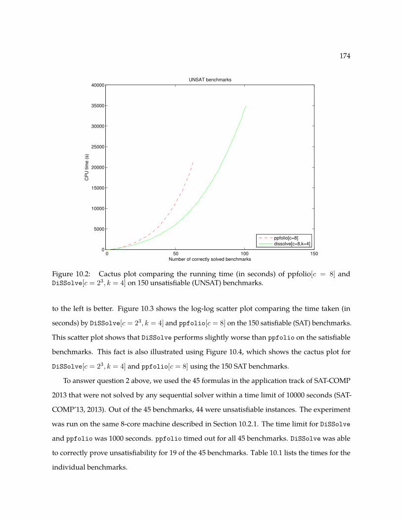
174
0 50 100 150 0
5000
10000
15000
20000
25000
30000
35000
40000UNSAT benchmarks
Number of correctly solved benchmarks
CP
U tim
e (
s)
ppfolio[c=8]
dissolve[c=8,k=4]
Figure 10.2: Cactus plot comparing the running time (in seconds) of ppfolio[c = 8] andDiSSolve[c = 23, k = 4] on 150 unsatisfiable (UNSAT) benchmarks.
to the left is better. Figure 10.3 shows the log-log scatter plot comparing the time taken (in
seconds) by DiSSolve[c = 23, k = 4] and ppfolio[c = 8] on the 150 satisfiable (SAT) benchmarks.
This scatter plot shows that DiSSolve performs slightly worse than ppfolio on the satisfiable
benchmarks. This fact is also illustrated using Figure 10.4, which shows the cactus plot for
DiSSolve[c = 23, k = 4] and ppfolio[c = 8] using the 150 SAT benchmarks.
To answer question 2 above, we used the 45 formulas in the application track of SAT-COMP
2013 that were not solved by any sequential solver within a time limit of 10000 seconds (SAT-
COMP’13, 2013). Out of the 45 benchmarks, 44 were unsatisfiable instances. The experiment
was run on the same 8-core machine described in Section 10.2.1. The time limit for DiSSolve
and ppfolio was 1000 seconds. ppfolio timed out for all 45 benchmarks. DiSSolve was able
to correctly prove unsatisfiability for 19 of the 45 benchmarks. Table 10.1 lists the times for the
individual benchmarks.
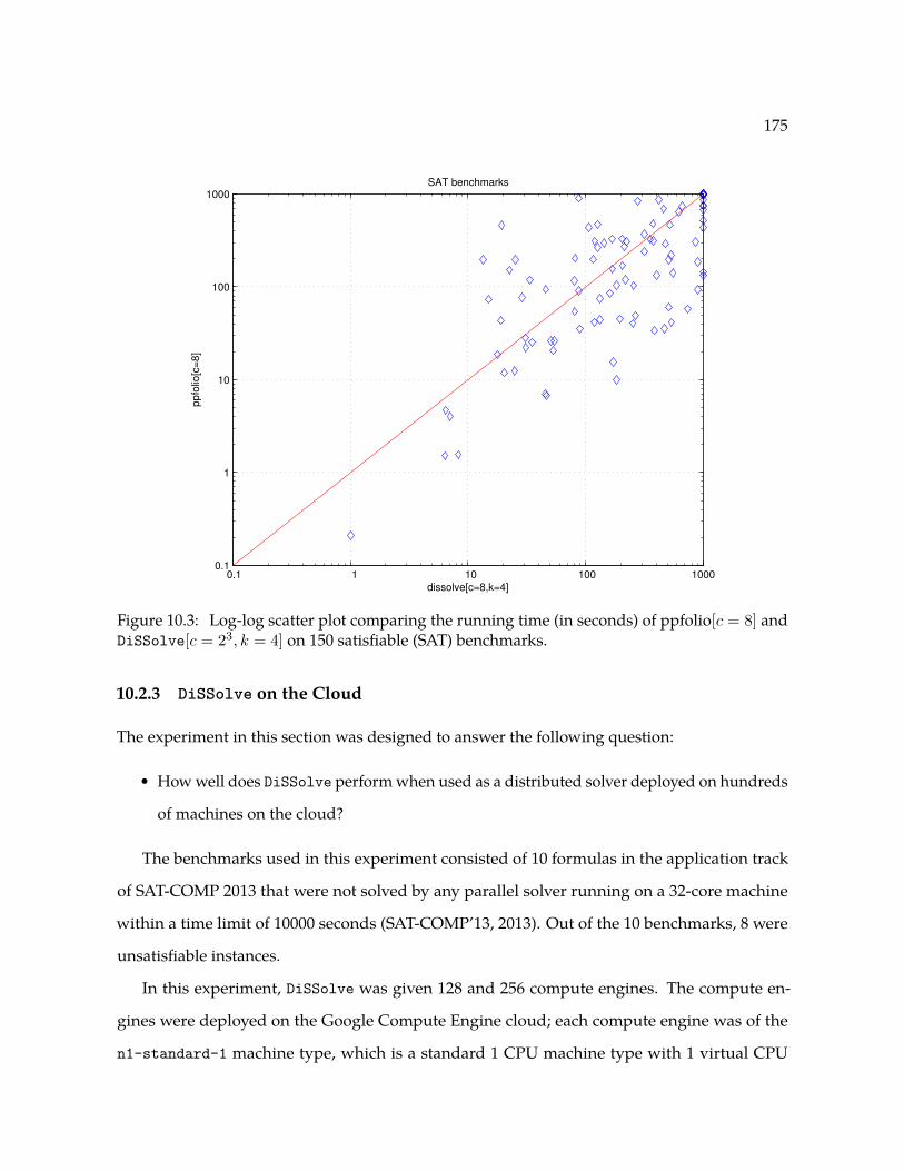
175
0.1 1 10 100 1000 0.1
1
10
100
1000SAT benchmarks
dissolve[c=8,k=4]
ppfo
lio[c
=8]
Figure 10.3: Log-log scatter plot comparing the running time (in seconds) of ppfolio[c = 8] andDiSSolve[c = 23, k = 4] on 150 satisfiable (SAT) benchmarks.
10.2.3 DiSSolve on the Cloud
The experiment in this section was designed to answer the following question:
• How well does DiSSolve perform when used as a distributed solver deployed on hundreds
of machines on the cloud?
The benchmarks used in this experiment consisted of 10 formulas in the application track
of SAT-COMP 2013 that were not solved by any parallel solver running on a 32-core machine
within a time limit of 10000 seconds (SAT-COMP’13, 2013). Out of the 10 benchmarks, 8 were
unsatisfiable instances.
In this experiment, DiSSolve was given 128 and 256 compute engines. The compute en-
gines were deployed on the Google Compute Engine cloud; each compute engine was of the
n1-standard-1 machine type, which is a standard 1 CPU machine type with 1 virtual CPU
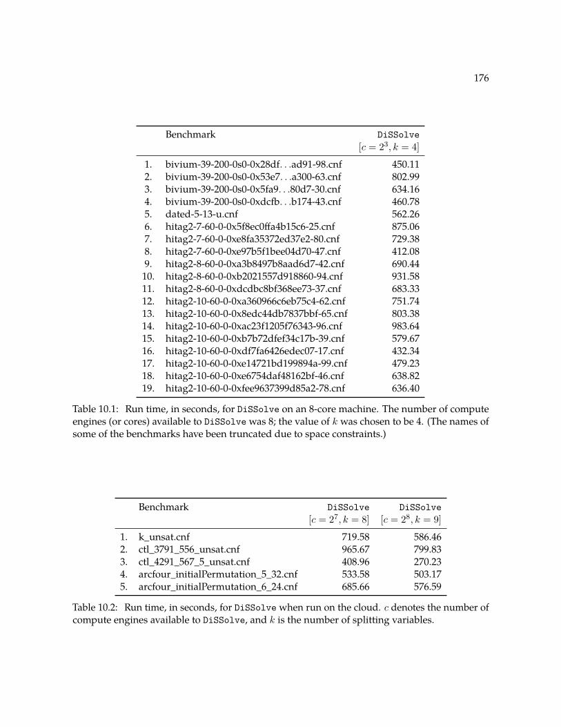
176
Benchmark DiSSolve[c = 23, k = 4]
1. bivium-39-200-0s0-0x28df. . .ad91-98.cnf 450.112. bivium-39-200-0s0-0x53e7. . .a300-63.cnf 802.993. bivium-39-200-0s0-0x5fa9. . .80d7-30.cnf 634.164. bivium-39-200-0s0-0xdcfb. . .b174-43.cnf 460.785. dated-5-13-u.cnf 562.266. hitag2-7-60-0-0x5f8ec0ffa4b15c6-25.cnf 875.067. hitag2-7-60-0-0xe8fa35372ed37e2-80.cnf 729.388. hitag2-7-60-0-0xe97b5f1bee04d70-47.cnf 412.089. hitag2-8-60-0-0xa3b8497b8aad6d7-42.cnf 690.44
10. hitag2-8-60-0-0xb2021557d918860-94.cnf 931.5811. hitag2-8-60-0-0xdcdbc8bf368ee73-37.cnf 683.3312. hitag2-10-60-0-0xa360966c6eb75c4-62.cnf 751.7413. hitag2-10-60-0-0x8edc44db7837bbf-65.cnf 803.3814. hitag2-10-60-0-0xac23f1205f76343-96.cnf 983.6415. hitag2-10-60-0-0xb7b72dfef34c17b-39.cnf 579.6716. hitag2-10-60-0-0xdf7fa6426edec07-17.cnf 432.3417. hitag2-10-60-0-0xe14721bd199894a-99.cnf 479.2318. hitag2-10-60-0-0xe6754daf48162bf-46.cnf 638.8219. hitag2-10-60-0-0xfee9637399d85a2-78.cnf 636.40
Table 10.1: Run time, in seconds, for DiSSolve on an 8-core machine. The number of computeengines (or cores) available to DiSSolve was 8; the value of k was chosen to be 4. (The names ofsome of the benchmarks have been truncated due to space constraints.)
Benchmark DiSSolve DiSSolve[c = 27, k = 8] [c = 28, k = 9]
1. k_unsat.cnf 719.58 586.462. ctl_3791_556_unsat.cnf 965.67 799.833. ctl_4291_567_5_unsat.cnf 408.96 270.234. arcfour_initialPermutation_5_32.cnf 533.58 503.175. arcfour_initialPermutation_6_24.cnf 685.66 576.59
Table 10.2: Run time, in seconds, for DiSSolve when run on the cloud. c denotes the number ofcompute engines available to DiSSolve, and k is the number of splitting variables.

177
0 50 100 150 0
5000
10000
15000
20000
25000SAT benchmarks
Number of correctly solved benchmarks
CP
U tim
e (
s)
ppfolio[c=8]
dissolve[c=8,k=4]
Figure 10.4: Cactus plot comparing the running time (in seconds) of ppfolio[c = 8] andDiSSolve[c = 23, k = 4] on 150 unsatisfiabile (UNSAT) benchmarks.
and 3.75 GB of memory available on the Google Compute Engine service. The time limit per
benchmark for DiSSolve was 1000 seconds. DiSSolve was able to correctly prove unsatisfiability
for 5 out of the 10 benchmarks. Table 10.2 lists the running times for the individual benchmarks.
The second and third columns in Table 10.2 list the time taken by DiSSolve when using 128 and
256 compute engines, respectively.
10.3 Generalization
In this section, I first describe a natural extension of DiSSolve from SAT to SMT. I then describe
the DiSSolveSplit function using abstract-interpretation terminology.
The DiSSolve algorithm described in Section 10.1 can be naturally generalized to handle
richer logics by replacing the SAT solver used to implement Deduce on line 4 with an SMT

178
Algorithm 22: AbstractDissolveSplit(ϕ,A)1 k = |V |2 {A1, A2, . . . , An} ← AbstractDilemmaAssumptions()3 for i ∈ {1, 2, . . . , n} do4 A′i ← Deduce(ϕ,A uAi)5 A′ ← A uA′0 uA′1 uA′2 . . . uA′2k−16 return A′
solver. Consequently, the set of clauses returned would not be over propositional literals, but
would instead contain literals of the particular theory. However, the algorithm as stated would
still apply to this new setting; in particular, the UnionClauses method could ignore the theory
interpretation of the literals, and the DiSSolveSplit method would remain sound. Furthermore,
instead of allowing arbitrary literals of the theory, we could restrict the set of literals to a fixed set
of predicates. In other words, we could use an abstract domain of clauses involving a fixed set of
predicates (which is one way to implement the abstract domain of full predicate abstraction).
The implementation of the DiSSolve algorithm described in Section 10.1 can be viewed as
using the m-clausal abstract domain; that is, an abstract domain of clauses of length up to m. The
meet of two abstract values is the union of the sets of clauses that correspond to the abstract
values.
Algorithm 22 presents the DiSSolveSplit function of Algorithm 21 using abstract-interpretation
terminology. An abstract value A from an abstract domain A plays the role of the set of clauses
C used in Algorithm 21. The function AbstractDilemmaAssumptions on line 2 returns a set of n
abstract values Ai such that⋃i γ(Ai) ⊇ γ(A). The function Deduce must return an abstract value
A′i such that ϕ⇒ γ(A′i) (line 4).1 Finally, on line 5, the abstract values returned by each call to
Deduce are merged by performing a meet (u).
Figures 10.5 and 10.6 illustrate the two distinct processes that occur in the calls to Deduce
on line 4, and shed light on the behavior of AbstractDissolveSplit in terms of the lattice of the
abstract domain A. Assume that AbstractDilemmaAssumptions returns two abstract values1 Note that, unlike Algorithm 18 and Figure 6.3(b), where A′i v Ai, at line 4 of Algorithm 22 A′i v Ai does not
hold, in general. The requirement on A′i is ϕ⇒ γ(A′i).
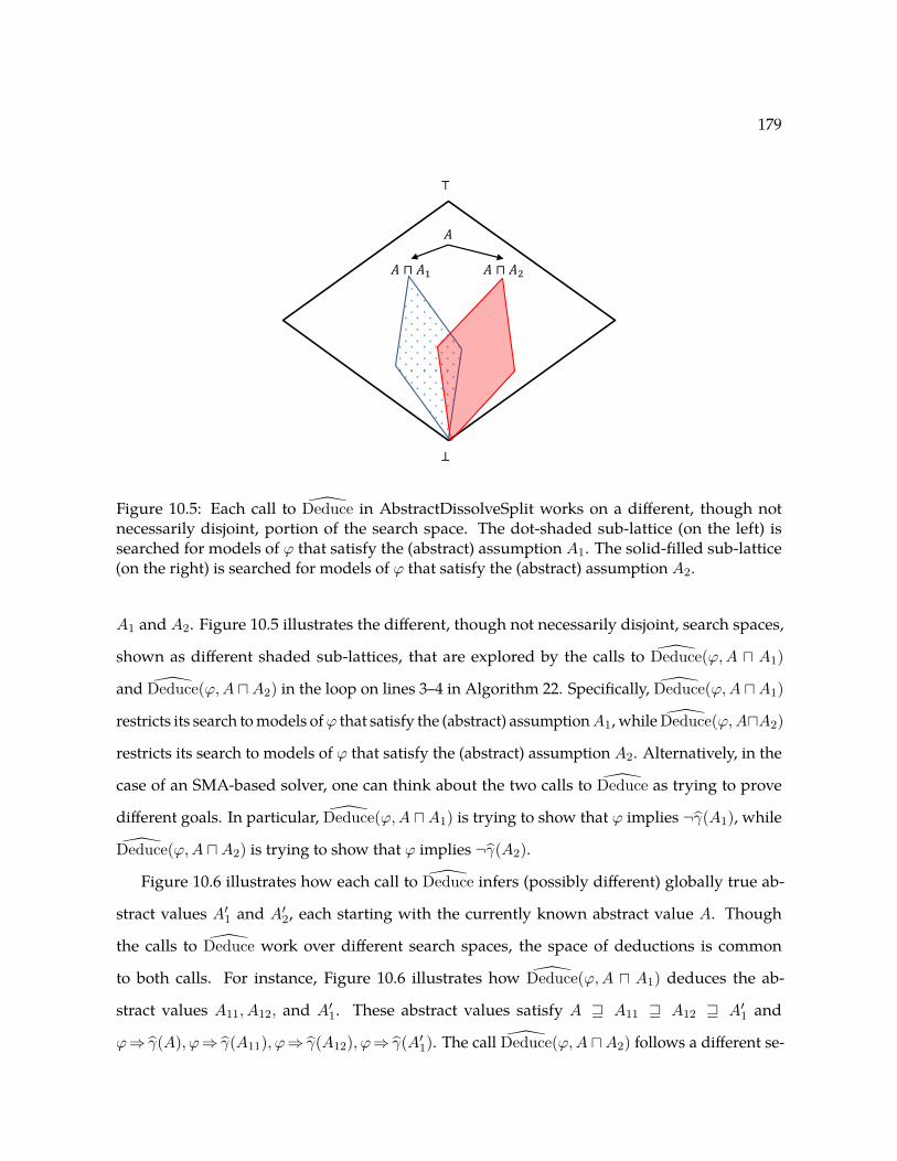
179
𝐴 ⊓ 𝐴1
⊥
𝐴 ⊓ 𝐴2
𝐴
⊤
Figure 10.5: Each call to Deduce in AbstractDissolveSplit works on a different, though notnecessarily disjoint, portion of the search space. The dot-shaded sub-lattice (on the left) issearched for models of ϕ that satisfy the (abstract) assumption A1. The solid-filled sub-lattice(on the right) is searched for models of ϕ that satisfy the (abstract) assumption A2.
A1 and A2. Figure 10.5 illustrates the different, though not necessarily disjoint, search spaces,
shown as different shaded sub-lattices, that are explored by the calls to Deduce(ϕ,A u A1)
and Deduce(ϕ,A uA2) in the loop on lines 3–4 in Algorithm 22. Specifically, Deduce(ϕ,A uA1)
restricts its search to models ofϕ that satisfy the (abstract) assumptionA1, while Deduce(ϕ,AuA2)
restricts its search to models of ϕ that satisfy the (abstract) assumption A2. Alternatively, in the
case of an SMA-based solver, one can think about the two calls to Deduce as trying to prove
different goals. In particular, Deduce(ϕ,A uA1) is trying to show that ϕ implies ¬γ(A1), while
Deduce(ϕ,A uA2) is trying to show that ϕ implies ¬γ(A2).
Figure 10.6 illustrates how each call to Deduce infers (possibly different) globally true ab-
stract values A′1 and A′2, each starting with the currently known abstract value A. Though
the calls to Deduce work over different search spaces, the space of deductions is common
to both calls. For instance, Figure 10.6 illustrates how Deduce(ϕ,A u A1) deduces the ab-
stract values A11, A12, and A′1. These abstract values satisfy A w A11 w A12 w A′1 and
ϕ⇒ γ(A), ϕ⇒ γ(A11), ϕ⇒ γ(A12), ϕ⇒ γ(A′1). The call Deduce(ϕ,A uA2) follows a different se-

180
𝐴𝐴11
⊥
𝐴𝐴21
𝐴𝐴
⊤
𝐴𝐴𝐴1 𝐴𝐴𝐴2
𝐴𝐴1′ ⊓ 𝐴𝐴𝐴2
𝐴𝐴12 𝐴𝐴22
Figure 10.6: Each call to Deduce in AbstractDissolveSplit infers (possibly different) globallytrue abstract values A′1 and A′2, where ϕ⇒ γ(A′1) and ϕ⇒ γ(A′2). These two branches are thenmerged by performing a meet.
quence of deductions to reach the abstract value A′2, where ϕ⇒ γ(A′2). Finally, the two branches
of the proof are then merged by performing the meet of A′1 and A′2.
10.4 Related Work
This section reflects only a small portion of the literature on sequential and parallel SAT solvers.
The introduction of this chapter already provided a qualitative comparison of DiSSolve with
modern parallel SAT solvers based on divide-and-conquer and parallel portfolio approaches.
Hamadi and Wintersteiger (2012) present an overview of parallel SAT solvers.
Katsirelos et al. (2013) explore bottlenecks to parallelization of SAT solvers. Their findings
suggest that efficient parallelization of SAT is not merely a matter of designing the right clause-
sharing heuristic. They suggest exploring solvers based on other proof systems that produce
more parallelizable refutations. This observation provided motivation for exploring a technique
that does not fall into the divide-and-conquer and parallel-portfolio approaches.

181
SatX10 (Bloom et al., 2012) is a framework for implementing parallel SAT solvers based
on the parallel execution language X10. The implementation of DiSSolve is written in the go
programming language (Go, 2014). The concurrency features built into go greatly simplified the
design and implementation of DiSSolve.
Audemard et al. (2012) explore techniques for clause exchanges within a parallel SAT solver
that incorporate the LBD heuristic developed for the Glucose sequential solver. They incorporate
these techniques in Penelope, a portfolio-based parallel SAT solver.
Hamadi et al. (2011) describe a lazy-decomposition technique for distributing formulas,
which is based on Craig interpolation. Instead of partitioning the search space, Hamadi et al.
(2011) partition the clauses of the problem formula. Such a partitioning technique is especially
useful when the input formula is too large to fit in main memory. This approach is orthogonal to
the search-space decomposition technique used in DiSSolve.
The technique of choosing partition variables as a weighted sum of the decision variables
returned by Deduce used in DiSSolve can also be found in Martins et al. (2010).
Currently, DiSSolve maintains a fixed bound on the number of clauses maintained, and the
number of clauses returned by each call to Deduce. Hamadi et al. (2009a) described a dynamic
control-based technique for guiding clause sharing.
10.5 Chapter Notes
Nick Kidd helped with the implementation of DiSSolve in the go programming language. He
also directed me to the book The Wisdom of Crowds from which the quotation for this chapter was
taken.
I had a great time learning how to use The Cloud.

182
Chapter 11
Satisfiability Modulo Abstraction for
Separation Logic with Linked Lists
This chapter describes a sound procedure for checking the unsatisfiability of formulas in a frag-
ment of separation logic. The procedure is designed using concepts from abstract interpretation,
and is thus a Satisfiability Modulo Abstraction (SMA) solver.
Separation logic (Reynolds, 2002) is an expressive logic for reasoning about heap-allocated
data structures in programs. It provides a mechanism for concisely describing program states by
explicitly localizing facts that hold in separate regions of the heap. In particular, a “separating
conjunction” (ϕ1 ∗ ϕ2) asserts that the heap can be split into two disjoint regions (“heaplets”)
in which ϕ1 and ϕ2 hold, respectively (Reynolds, 2002). A “septraction” (ϕ1 −~ ϕ2) asserts
that a heaplet h can be extended by a disjoint heaplet h1 in which ϕ1 holds, to create a heaplet
h1 ∪ h in which ϕ2 holds (Vafeiadis and Parkinson, 2007). The −~ operator is sometimes called
existential magic wand, because it is the DeMorgan-dual of the magic-wand operator “−∗” (also
called separating implication); i.e., ϕ1 −~ ϕ2 iff ¬(ϕ1 −∗ ¬ϕ2).
The use of separation logic in manual, semi-automated, and automated verification tools is a
burgeoning field (Berdine et al., 2005; Distefano et al., 2006; Magill et al., 2007; Distefano and
Parkinson, 2008; Dudka et al., 2013). Most of these incorporate some form of automated reasoning
for separation logic, but only limited fragments of separation logic are typically handled.
183
Given a formula ϕ, the unsatisfiability checker sets up an appropriate abstract domain that is
tailored for representing information about the meanings of subformulas of ϕ. It uses an abstract
domain of shape graphs (Sagiv et al., 2002) to represent a set of heap structures. The proof
calculus that is presented performs a bottom-up evaluation of ϕ, using a particular shape-graph
interpretation. It computes an abstract value that over-approximates the set of satisfying models
of ϕ. If the over-approximation is the empty set of shape graphs, then ϕ is unsatisfiable. If ϕ is
satisfiable, then the procedure reports a set of abstract models.
The unsatisfiability checker presented in this chapter is the first to apply the SMA approach
to a fragment of separation logic. One of the main advantages of the SMA approach is that it is
able to reuse abstract-interpretation machinery to implement decision procedures. In Chapter 6,
for instance, the polyhedral abstract domain—implemented in PPL (Bagnara et al., 2008)—is
used to implement a decision procedure for the logic of linear rational arithmetic. In this chapter,
the abstract domain of shapes—implemented in TVLA (Sagiv et al., 2002)—is used in a novel
way to implement a sound procedure for checking unsatisfiability of formulas in separation
logic. The challenge was to instantiate the parametric framework of TVLA to precisely represent
the literals and capture the spatial constraints of our fragment of separation logic.
The nature of this unsatisfiability checker is thus much different from other decision proce-
dures for fragments of separation logic that I are aware of. Most previous decision procedures
are proof-theoretic. In some sense, our method is model-theoretic: it uses explicitly instantiated sets
of 3-valued structures to represent overapproximations of the models of subformulas.
The fragment of separation logic discussed in this chapter includes points-to assertions (x 7→
y), acyclic-list-segment assertions (ls(x, y)), empty-heap assertions (emp), and their negations;
separating conjunction; septraction; logical-and; and logical-or. The fragment considered only
allows negation at the leaves of a formula (Section 11.1.1), but still contains formulas that lie
outside of previously considered fragments (Berdine et al., 2004; Pérez and Rybalchenko, 2011;
Park et al., 2013; Lee and Park, 2014; Hou et al., 2014). The procedure can prove validity of

184
implications of the form
ψ⇒(ϕi ∧∧j
ψj −∗ ϕj), (11.1)
where ϕi and ϕj are formulas that contain only ∧, ∨, and positive or negative occurrences of emp,
points-to, or ls assertions; and ψ and ψj are arbitrary formulas in the logic fragment defined in
Section 11.1.1. Consequently, we believe that ours is the first procedure that can prove the validity
of formulas that contain both ls and the magic-wand operator −∗. Furthermore, the procedure
is able to prove unsatisfiability of interesting classes of formulas that are outside of previously
considered fragments, including (i) formulas that use conjunctions of separating-conjunctions with
ls or negations below separating-conjunctions, such as
(ls(a1, a2) ∗ ls(a2, a3)) ∧ (¬emp ∗ ¬emp)
∧(a1 7→ e1 ∗ True) ∧ e1 = nil,
and (ii) formulas that contain both ls and septraction (−~), such as
(a3 7→ a4−~ ls(a1, a4)) ∧ (a3 = a4 ∨ ¬ls(a1, a3)).
The former are useful for describing overlaid data structures; the latter are useful in dealing with
interference effects when using rely/guarantee reasoning to verify programs with fine-grained
concurrency (Vafeiadis and Parkinson, 2007; Calcagno et al., 2007).
The contributions of this chapter include the following:
• I show how a canonical-abstraction domain can be used to overapproximate the set of
heaps that satisfy a separation-logic formula (Section 11.1).
• I present rules for calculating the overapproximation of a separation-logic formula for a
fragment of separation logic that consists of separating conjunction, septraction, logical-and,
and logical-or (Section 11.3).
• The procedure is parameterized by a shape abstraction, and can be instantiated to handle
(positive or negative) literals for points-to or acyclic-list-segment assertions—and hence
can prove the validity of implications of the kind shown in formula (11.1) (Section 11.3).

185
Section 11.2 illustrates the key concepts used in the unsatisfiability-checking procedure. The pro-
cedure is implemented in a tool called SMASLTOV (Satisfiability Modulo Abstraction for Separa-
tion Logic ThrOugh Valuation), which is available at https://www.github.com/smasltov-team/
SMASLTOV. I evaluated SMASLTOV on a set of formulas taken from the literature (Section 11.4).
To the best of my knowledge, SMASLTOV is able to establish the unsatisfiability of formulas that
cannot be handled by previous approaches.
11.1 Separation Logic and Canonical Abstraction
In this section, I provide background on separation logic and introduce the separation-logic
fragment considered in the thesis. I then show how a canonical-abstraction domain can be used
to approximate the set of models that satisfy a separation-logic formula.
11.1.1 Syntax and Semantics of Separation Logic
Formulas in our fragment of separation logic (SL) are defined as follows:
ϕ ::= ϕ ∧ ϕ | ϕ ∨ ϕ | ϕ ∗ ϕ | ϕ−~ ϕ | atom | ¬atom
atom ::= true | emp | x = y | x 7→ y | ls(x, y)
The set of literals, denoted by Literals, is the union of the positive and negative atoms of SL.
The semantics of SL is defined with respect to memory “statelets”, which consist of a store
and a heaplet. A store is a function from variables to values; a heaplet is a finite function from
locations to locations.
Val def= Loc ] {nil} Store def= Var→ Val
Heaplet def= Loc ⇀fin Val Statelet def= Store×Heaplet
Loc and Var are disjoint countably infinite sets, neither of which contain nil. Loc represents
heap-node addresses. The domain of h, dom(h), represents the set of addresses of cells in the
heaplet. Two heaplets h1, h2 are disjoint, denoted by h1#h2, if dom(h1) ∩ dom(h2) = ∅. Given
two disjoint heaplets h1 and h2, h1 · h2 denotes their disjoint union h1 ] h2. A statelet is denoted
by a pair (s, h).

186
(s, h) |= ϕ1 ∧ ϕ2 iff (s, h) |= ϕ1 and (s, h) |= ϕ2(s, h) |= ϕ1 ∨ ϕ2 iff (s, h) |= ϕ1 or (s, h) |= ϕ2(s, h) |= ϕ1 ∗ ϕ2 iff ∃h1, h2. h1#h2 and h1 · h2 = h and
(s, h1) |= ϕ1 and (s, h2) |= ϕ2(s, h) |= ϕ1 −~ ϕ2 iff ∃h1. h1#h and (s, h1) |= ϕ1 and
(s, h1 · h) |= ϕ2(s, h) |= ¬atom iff (s, h) 6|= atom(s, h) |= true iff true(s, h) |= emp iff dom(h) = ∅(s, h) |= x = y iff s(x) = s(y)(s, h) |= x 7→ y iff dom(h) = {s(x)} and h(s(x)) = s(y)(s, h) |= ls(x, y) iff if s(x) = s(y) then dom(h) = ∅,
else there is a nonempty acyclic path froms(x) to s(y) in h, and this path containsall heap cells in h
Figure 11.1: Satisfaction of an SL formula ϕ with respect to statelet (s, h).
Satisfaction of an SL formula ϕ with respect to statelet (s, h) is defined in Figure 11.1. Fur-
thermore, in this chapter, we consider a formula to be satisfiable only if it is satisfiable over an
acyclic heap. JϕK denotes the set of statelets that satisfy ϕ: JϕK def= {(s, h) | (s, h) |= ϕ}.
11.1.2 2-Valued Logical Structures
We model full states—not statelets—by 2-valued logical structures. A logical structure provides an
interpretation of a vocabulary Voc = {eq, p1, . . . , pn} of predicate symbols (with given arities).
Vock denotes the set of k-ary symbols.
Definition 11.1. A 2-valued logical structure S over Voc is a pair S = 〈U, ι〉, where U is the
set of individuals, and ι is the interpretation. Let B = {0, 1} be the domain of truth values.
For p ∈ Voci, ι(p) : U i → B. We assume that eq ∈ Voc2 is the identity relation: (i) for all
u ∈ U , ι(eq)(u, u) = 1, and (ii) for all u1, u2 ∈ U such that u1 and u2 are distinct individuals,
ι(eq)(u1, u2) = 0.
The set of 2-valued logical structures over Voc is denoted by 2-STRUCT[Voc]. �
A concrete state is modeled by a 2-valued logical structure over a fixed vocabulary C of core
predicates. Core predicates are part of the underlying semantics of the linked structures that make

187
Predicate Intended Meaning
eq(v1, v2) Do v1 and v2 denote the same memory cell?q(v) Does pointer variable q point to memory cell v?n(v1, v2) Does the n-field of v1 point to v2?
Table 11.1: Core predicates used when representing states made up of acyclic linked lists.
up the states of interest. Table 11.1 lists the core predicates that are used when representing
states made up of acyclic linked lists.
Without loss of generality, vocabularies exclude constant and function symbols. Constant
symbols can be encoded via unary predicates, and n-ary functions via n + 1-ary predicates.
In both cases, we need integrity rules—i.e., global constraints that restrict the set of structures
considered to the ones that we intend. The set of unary predicates, Voc1, always contains
predicates that encode the variables of the formula. In a minor abuse of notation, we overload
“x” to denote both the name of variable x and the unary predicate x(·) that encodes the variable.
The binary predicate n ∈ Voc2 encodes list-node linkages. In essence, the following integrity
rules restrict each x ∈ Var ⊆ Voc1 to serve as a constant, and restrict relation n to encode a partial
function:
for each x ∈ Var, ∀v1, v2 : x(v1) ∧ x(v2) ⇒ eq(v1, v2)
∀v1, v2, v3 : n(v3, v1) ∧ n(v3, v2) ⇒ eq(v1, v2)
11.1.3 Connecting 2-Valued Logical Structures and SL Statelets
We use unary domain predicates, typically denoted by d, d′, d1, . . . , dk ∈ Voc1, to pick out regions of
the heap that are of interest in the state that a logical structure models. The connection between
2-valued logical structures and SL statelets is formalized by means of the operation S|(d,·), which

188
performs a projection of structure S with respect to a domain predicate d:
S|(d,·)def= (s, h),where
s =
{(p, u) | p ∈ VarS , u ∈ US , and p(u)}
∪ {(q, nil) | q ∈ VarS and ¬∃v : q(v)}
(11.2)
h = {(u1, u2) | u1, u2 ∈ US , d(u1), and n(u1, u2)}. (11.3)
The subscript “(d, ·)” serves as a reminder that in Equation (11.3), only u1 needs to be in the
region defined by d. We lift the projection operation to apply to a set SS of 2-valued logical
structures as follows:
SS|(d,·)def= {S|(d,·) | S ∈ SS}.
11.1.4 Representing Sets of SL Statelets using Canonical Abstraction
In the framework of Sagiv et al. (2002) for logic-based abstract-interpretation, 3-valued logical
structures provide a way to overapproximate possibly infinite sets of 2-valued structures in a
finite way that can be represented in a computer. The application of Equations (11.2) and (11.3)
to 3-valued structures means that the abstract-interpretation machinery developed by Sagiv et
al. provides a finite way to overapproximate a possibly infinite set of SL statelets.
In 3-valued logic, a third truth value, denoted by 1/2, represents uncertainty. The set T def=
B ∪ {1/2} of 3-valued truth values is partially ordered “l @ 1/2 for l ∈ B”. The values 0 and 1
are definite values; 1/2 is an indefinite value.
Definition 11.2. A 3-valued logical structure S = 〈U, ι〉 is almost identical to a 2-valued struc-
ture, except that ι maps each p ∈ Voci to a 3-valued function ι(p) : U i → T. In addition, (i) for
all u ∈ U , ι(eq)(u, u) w 1, and (ii) for all u1, u2 ∈ U such that u1 and u2 are distinct individuals,
ι(eq)(u1, u2) = 0. (An individual u for which ι(eq)(u, u) = 1/2 is called a summary individual.)
The set of 3-valued logical structures over Voc is denoted by 3-STRUCT[Voc]. Note that
2-STRUCT[Voc] ( 3-STRUCT[Voc]. �

189
As we will see below, a summary individual may represent more than one individual from
certain 2-valued structures.
A 3-valued structure can be depicted as a directed graph with individuals as graph nodes (see
Figure 11.2). A summary individual is depicted with a double-ruled border. A unary predicate
p ∈ Var is represented in the graph by having an arrow from the predicate name p to all nodes
of individuals u for which ι(p)(u) w 1. An arrow between two nodes indicates that a binary
predicate holds for the corresponding pair of individuals. (To reduce clutter, in the figures in
this chapter, the only binary predicate shown is the predicate n ∈ Voc2.) A predicate value of
1/2 is indicated by a dotted arrow, a value of 1 by a solid arrow, and a value of 0 by the absence
of an arrow. A unary predicate p ∈ (Voc1 − Var) is listed, with its value, inside the node of each
individual u for which ι(p)(u) w 1. A nullary predicate is displayed in a rectangular box.
To define a suitable abstraction of 2-valued logical structures, we start with the notion of
structure embedding (Sagiv et al., 2002):
Definition 11.3. Given S = 〈U, ι〉 and S′ = 〈U ′, ι′〉, two 3-valued structures over the same
vocabulary Voc, and f : U → U ′, a surjective function, f embeds S in S′, denoted by S vf S′, if
for all p ∈ Voc and u1, . . . , uk ∈ U ,
ι(p)(u1, . . . , uk) v ι′(p)(f(u1), . . . , f(uk))
If, in addition,
ι′(p)(u′1, . . . , u′k) =⊔
u1,...,uk∈U,s.t.f(ui)=u′i,1≤i≤kι(p)(u1, . . . , uk)
then S′ is the tight embedding of S with respect to f , denoted by S′ = f(S). (Note that
we overload f to also mean the mapping on structures f : 3-STRUCT[Voc] → 3-STRUCT[Voc]
induced by f : U → U ′.) �
Intuitively, f(S) is obtained by merging individuals of S and by defining the valuation of
predicates accordingly (in the most precise way). The relation vid, which will be denoted by
v, is the natural information order between structures that share the same universe. One has
S vf S′ ⇔ f(S) vid S′. Henceforth, we use S vf S′ to mean “there exists a surjective f : U → U ′
such that f(S) vid S′”.

190
However, embedding alone is not enough. The challenge for representing and manipulating
sets of 2-valued structures is that the universe of a structure is of a priori unbounded size.
Consequently, we need a method that, for a 2-valued structure 〈U, ι〉 ∈ 2-STRUCT[Voc], abstracts
U to an abstract universe U ] of bounded size. The idea behind canonical abstraction (Sagiv
et al., 2002, Section 4.3) is to choose a subset A ⊆ Voc1 of abstraction predicates, and to define
an equivalence relation 'AS on U that is parameterized by the logical structure S = 〈U, ι〉 ∈
2-STRUCT[Voc] to be abstracted:
u1 'AS u2 ⇔ ∀p ∈ A : ι(p)(u1) = ι(p)(u2).
This equivalence relation defines the surjective function fSA : U → (U/ 'AS ), which maps an
individual to its equivalence class. We thus have the Galois connection
℘(2-STRUCT[Voc]) −−→←−−αγ
℘(3-STRUCT[Voc])
α(X) = {fSA (S) | S ∈ X}
γ(Y ) = {S | S] ∈ Y ∧ S vf S]}
where fSA in the definition of α denotes the tight-embedding function for logical structures
induced by the node-embedding function fSA : U → (U/ 'AS ). The abstraction function α is
referred to as canonical abstraction. Note that there is an upper bound on the size of each structure
〈U ], ι]〉 ∈ 3-STRUCT[Voc] that is in the image of α: |U ]| ≤ 2|A|—and thus the power-set of the
image of α is a finite sublattice of ℘(3-STRUCT[Voc]).
For technical reasons, it turns out to be convenient to work with 3-valued structures other
than the ones in the image of α; however, we still want to restrict ourselves to a finite sublattice of
℘(3-STRUCT[Voc]). With this motivation, we make the following definition (Arnold et al., 2006):
Definition 11.4. A 3-valued structure 〈U ], ι]〉 ∈ 3-STRUCT[Voc] is bounded (with respect to
abstraction predicates A) if for every u1, u2 ∈ U ], where u1 6= u2, there exists an abstraction

191
predicate symbol p ∈ A ⊆ Voc1 such that ι](p)(u1) = 0 and ι](p)(u2) = 1, or ι](p)(u1) = 1 and
ι](p)(u2) = 0. B-STRUCT[Voc,A] denotes the set of such structures. �
Definition 11.4 also imposes an upper bound on the size of a structure 〈U ], ι]〉 ∈ B-STRUCT[Voc,A]—
again, |U ]| ≤ 2|A|—and thus ℘(B-STRUCT[Voc,A]) is a finite sublattice of ℘(3-STRUCT[Voc]).
It defines the abstract domain that we use, the abstract domain whose elements are subsets of
B-STRUCT[Voc,A], which will be denoted by A[Voc,A]. (For brevity, we call such a domain
a “canonical-abstraction domain”, and denote it by Awhen Voc and A are understood.) The Galois
connection we work with is thus
℘(2-STRUCT[Voc]) −−→←−−αγ
℘(B-STRUCT[Voc,A]) = A[Voc,A]
α(X) = {fSA (S) | S ∈ X}
γ(Y ) = {S | S] ∈ Y ∧ S vf S]}.
The ordering on ℘(B-STRUCT[Voc,A]) = A[Voc,A] is the Hoare ordering: S1 v S2 if for all
s1 ∈ S1 there exists s2 ∈ S2 such that s1 vf s2.
11.2 Overview
This section presents two examples to illustrate the concepts that we use in the unsatisfiability-
checking procedure:
• a formula that is unsatisfiable over acyclic linked lists: (x 7→ y) ∗ (y 7→ x)
• a formula that is satisfiable over acyclic linked lists: (x 7→ y)−~ ls(x, z).
11.2.1 An Unsatisfiable Formula
Consider ϕ def= x 7→ y ∗ y 7→ x. We want to compute A ∈ A such that γ(A)|(d,·) ⊇ JϕK. The key to
handling the ∗ operator is to introduce two new domain predicates d1 and d2, which are used to
demarcate the heaplets that must satisfy ϕ1def= x 7→ y and ϕ2
def= y 7→ x, respectively. We have

192
x y
d,d1,¬d2 d,¬d1, d2
¬d,¬d1,¬d2
r[n,x]
¬r[n,y]
next[n,y]d1
x y
¬d1
¬is_eq[x,y]()
¬r[n,x]
r[n,y]next[n,x]d2
x y
¬d2
¬is_eq[x,y]()
(a) (b) (c)
x y
d,d1,¬d2d,¬d1, d2
¬d,¬d1,¬d2
r[n,x]
¬r[n,y]
next[n,y]
¬is_eq[x,y]()
x y
d,d1,¬d2 d,¬d1, d2
¬d,¬d1,¬d2
r[n,x]
¬r[n,y]
next[n,y]
¬r[n,x]
r[n,y]next[n,x]
¬is_eq[x,y]()
x y
d,d1,¬d2 d,¬d1, d2
¬d,¬d1,¬d2
r[n,x]
¬r[n,y]
next[n,y]
¬r[n,x]
r[n,y]next[n,x]
¬is_eq[x,y]()
(d) (e) (f)
Figure 11.2: Structures that arise in the meet operation used to analyze x 7→ y ∗ y 7→ x.
designed A so that there exist A1, A2 ∈ A such that γ(A1)|(d1,·) = Jx 7→ yK and γ(A2)|(d2,·) =
Jy 7→ xK, respectively. Table 11.2 describes the abstraction predicates we use. A1 and A2 each
consist of a single 3-valued structure, shown in Figure 11.2(b) and Figure 11.2(c), respectively.
Furthermore, to satisfy ϕ1 ∗ ϕ2, d1 and d2 are required to be disjoint regions whose union is
d. A also contains an abstract value, which we will call D, that represents this disjointness
constraint exactly. D consists of four 3-valued structures. Figure 11.2(a) shows the “most general”
of them: it represents two disjoint regions, d1 and d2, that partition the d region (where each of d1
and d2 contain at least one cell). The summary individual labeled ¬d,¬d1,¬d2 in Figure 11.2(a)
represents a region that is disjoint from d. (See also Figure 11.6.)
Note that here and throughout the paper, for brevity the figures only show predicates that
are relevant to the issue under discussion.
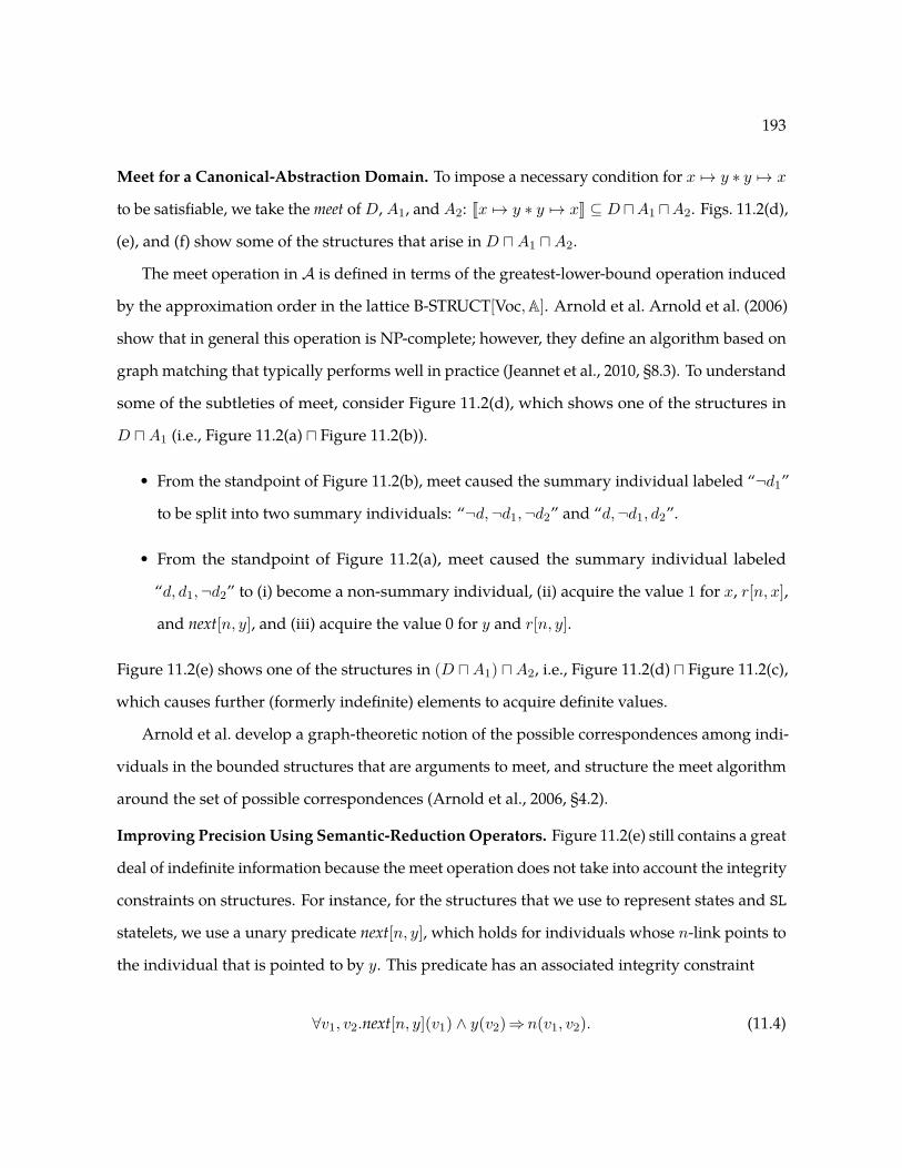
193
Meet for a Canonical-Abstraction Domain. To impose a necessary condition for x 7→ y ∗ y 7→ x
to be satisfiable, we take the meet of D, A1, and A2: Jx 7→ y ∗ y 7→ xK ⊆ DuA1 uA2. Figs. 11.2(d),
(e), and (f) show some of the structures that arise in D uA1 uA2.
The meet operation in A is defined in terms of the greatest-lower-bound operation induced
by the approximation order in the lattice B-STRUCT[Voc,A]. Arnold et al. Arnold et al. (2006)
show that in general this operation is NP-complete; however, they define an algorithm based on
graph matching that typically performs well in practice (Jeannet et al., 2010, §8.3). To understand
some of the subtleties of meet, consider Figure 11.2(d), which shows one of the structures in
D uA1 (i.e., Figure 11.2(a) u Figure 11.2(b)).
• From the standpoint of Figure 11.2(b), meet caused the summary individual labeled “¬d1”
to be split into two summary individuals: “¬d,¬d1,¬d2” and “d,¬d1, d2”.
• From the standpoint of Figure 11.2(a), meet caused the summary individual labeled
“d, d1,¬d2” to (i) become a non-summary individual, (ii) acquire the value 1 for x, r[n, x],
and next[n, y], and (iii) acquire the value 0 for y and r[n, y].
Figure 11.2(e) shows one of the structures in (D uA1) uA2, i.e., Figure 11.2(d) u Figure 11.2(c),
which causes further (formerly indefinite) elements to acquire definite values.
Arnold et al. develop a graph-theoretic notion of the possible correspondences among indi-
viduals in the bounded structures that are arguments to meet, and structure the meet algorithm
around the set of possible correspondences (Arnold et al., 2006, §4.2).
Improving Precision Using Semantic-Reduction Operators. Figure 11.2(e) still contains a great
deal of indefinite information because the meet operation does not take into account the integrity
constraints on structures. For instance, for the structures that we use to represent states and SL
statelets, we use a unary predicate next[n, y], which holds for individuals whose n-link points to
the individual that is pointed to by y. This predicate has an associated integrity constraint
∀v1, v2.next[n, y](v1) ∧ y(v2)⇒n(v1, v2). (11.4)
194
In particular, in Figure 11.2(e) the individual pointed to by x has next[n, y] = 1; however, the
edge to the individual pointed to by y has the value 1/2. Similarly, we force the procedure to
consider only acyclic heaps by imposing the integrity constraint ¬∃v1, v2.n(v1, v2) ∧ t[n](v2, v1).
To improve the precision of the (graph-theoretic) meet, the procedure makes use of semantic-
reduction operators. The notion of semantic reduction was introduced by Cousot and Cousot
Cousot and Cousot (1979). Semantic-reduction operators are useful when an abstract domain is
a lattice that has multiple elements that represent the same set of states. A semantic reduction
operator ρ maps an abstract-domain element A to ρ(A) such that (i) ρ(A) v A, and (ii) γ(ρ(A)) =
γ(A). In other words, ρ maps A to an element that is lower in the lattice—and hence a “better”
representation of γ(A) inA—while preserving the meaning. In our case, the semantic-reduction
operations that we use convert a set of 3-valued structures XS into a “better” set of 3-valued
structures XS ′ that describe the same set of 2-valued structures.
A semantic-reduction operator can have two effects:
1. In some structure S ∈ XS, some tuple p(u) with indefinite value 1/2 may be changed to
have a definite value (0 or 1).
2. It may be determined that some structure S ∈ XS is infeasible: i.e., γ(S) = ∅. In this case,
S is removed from XS.
The effect of a precision improvement from a type-1 effect can cause a type-2 effect to occur. For
instance, let u1 and u2 be the individuals pointed to by x and y, respectively, in Figure 11.2(e).
• Figure 11.2(f) is Figure 11.2(e) after integrity constraint (11.4) has triggered a type-1 change
that improves the value of n(u1, u2) from 1/2 to 1.
• A type-2 rule can then determine that the structure shown in Figure 11.2(f) is infeasible. In
particular, the predicate r[n, x](v) means that individual v is reachable from the individual
pointed to by x along n-links. The semantic-reduction rule would find that the values
x(u1) = 1, n(u1, u2) = 1, and r[n, x](u2) = 0 represent an irreconcilable inconsistency in

195
� �
¬��� �, �
���� �, �
¬� �, �
�¬� _�[�, �]()
(a)
���� ��, �, �
¬��� �,
������ ��, �,
¬� �,
� �, ��
¬� �,
�¬� _��[, ]()
(b)
� �
¬�
¬��¬��
���
¬��
��¬�
��
�
(c)
���� �, �, ����� �, �, �
�
�, ��, ��, ¬����� ��, �,
¬ �,
�,
¬ �, �
�,
¬ �, �
�, ¬��, � �, ¬�� , �
¬�
¬��
¬�
�¬��_��[�, ]()
¬��_��[�, �]()
(d)
���� �, �, � ���� �, �, �
�
�,
¬ �, �
�,
¬ �, �
� �
¬�
�¬��_�� �,
¬��_��[�, �]()
(e)
Figure 11.3: Some of the structures that arise in the meet operation used to evaluate x 7→y −~ ls(x, z).
Figure 11.2(f): the first two predicate values mean that u2 is reachable from the individual
pointed to by x along n-links, which contradicts r[n, x](u2) = 0.
The operation that applies type-1 and type-2 rules until no more changes are possible is called
coerce (because it coerces XS to a better representation XS ′). Sagiv et al. (Sagiv et al., 2002, §6.4)
and Bogudlov et al. Bogudlov et al. (2007a,b) discuss algorithms for coerce.
11.2.2 A Satisfiable Formula
Consider the formula ϕ def= x 7→ y −~ ls(x, z). We want to compute A ∈ A such that γ(A)|(d,·) ⊇
JϕK. Similar to what was done in Section 11.2.1 for the ∗ operator, we introduce two new domain
predicates d1 and d2, which are used to demarcate the heaplets that must satisfy ϕ1def= x 7→ y
and ϕ2def= ls(x, z). By design, there exist A1, A2 ∈ A such that γ(A1)|(d1,·) = Jx 7→ yK and
γ(A2)|(d2,·) = Jls(x, z)K, respectively. A1 consists of the single 3-valued structure shown in

196
Figure 11.3(a). Figure 11.3(b) shows one of the structures in A2; it represents an acyclic linked list
from x to z whose length is greater than 1. Furthermore, to satisfy ϕ1−~ϕ2, d and d1 are required
to be disjoint regions whose union is d2. A also contains an abstract value, which we will call
D, that represents this disjointness constraint exactly. D consists of four 3-valued structures.
Figure 11.3(c) shows the “most general” of them: it represents two disjoint regions, d and d1,
that partition the d2 region (where each of d and d1 contain at least one cell). The summary
individual labeled ¬d,¬d1,¬d2 in Figure 11.3(c) represents a region that is disjoint from d2.
To impose a necessary condition for x 7→ y −~ ls(x, z) to be satisfiable, we take the meet of D,
A1, and A2: Jx 7→ y −~ ls(x, z)K ⊆ D uA1 uA2. Figure 11.3(d) shows one of the structures that
arises in D uA1 uA2, after the semantic-reduction operators have been applied. A few points to
note about this resultant structure:
• The summary individual in region d2 present in the ls(x, z) structure in Figure 11.3(b) is
split in Figure 11.3(d) into a singleton individual pointed to by y and a summary individual.
• The individual pointed to by x is in regions d1 and d2, but not d.
• The individual pointed to by y is in regions d and d2, but not d1.
• The variables x and y are not equal.
• All the individuals in d are reachable from y, not reachable from z, and have link[d, n, z]
true.
Figure 11.3(e) shows the structure after we have projected the heap onto the heap region d;
that is, the values of the domain predicates d1 and d2 have been set of 1/2 on all individuals,
and all the abstraction predicates have been set to 1/2 on all individuals not in d. In effect, this
operation blurs the distinction between the region that is outside d, but in d2, and the region
that is outside of d and d2. Note that the fact that x and y are not equal is preserved by the
projection operation. This projection operation, denoted by (·) d in Section 11.3, serves as an
abstract method for quantifier elimination.

197
` ∈ Literals, d A`(`)
ϕ1, d A1 ϕ2, d A2
ϕ1 ∧ ϕ2, d A1 uA2(∧)
ϕ1, d S1 ϕ2, d A2
ϕ1 ∨ ϕ2, d A1 tA2(∨)
ϕ1, d1 A1 ϕ2, d2 A2
ϕ1 ∗ ϕ2, d ([d = d1 · d2]] uA1 uA2) d(∗)
ϕ1, d1 A1 ϕ2, d2 A2
ϕ1 −~ ϕ2, d ([d2 = d · d1]] uA1 uA2) d(−~)
Figure 11.4: Rules for computing an abstract value that overapproximates the meaning of aformula in SL
.
Predicate Intended Meaning
is_eq[x, y]() Are x and y equal?next[n, y](v) The target of the n-edge from v is
pointed to by yt[n](v1, v2) Is v2 reachable via zero or more
n-edges from v1?r[n, y](v) ∃v1.y(v1) ∧ t[n](v1, v)d(v) Is v in heap domain d?link[d, n, y](v) The target of the n-edge from v is
either in d or is pointed to by y
Table 11.2: Voc consists of the predicates shown above, together with the ones in Table 11.1. Allunary predicates are abstraction predicates; that is, A = Voc1.
Note that Figure 11.3(e) represents an acyclic linked-list from y to z with x 6= y, which is one
of the models that satisfies x 7→ y −~ ls(x, z).
11.3 Proof System for Separation Logic
This section describes how we compute A ∈ A[Voc,A] such that A overapproximates the satisfy-
ing models of ϕ ∈ SL. The vocabulary Voc and abstraction predicates A are listed in Table 11.2.
The procedure works with judgments of the form “ϕ, d A”, where d is a domain predicate.
The invariant maintained by the procedure is that, whenever it establishes a judgment ϕ, d A,
A ∈ A overapproximates ϕ in the following sense: γ(A)|(d,·) ⊇ JϕK. Figure 11.4 lists the rules
used for calculating ϕ, d A for ϕ ∈ SL. Using these rules, the procedure performs a bottom-up

198
� �
¬�
��_�[�, �]()
(a)
� �
¬�� �, �
���� �, �
¬� �, �
¬�_� [�, �]()
(b)
���� �, �, �
� �
¬�
�, �
����� �, �, �
¬ �, �
�, ��
¬ �, �
¬��_ �[�, �]()
(c)
Figure 11.5: The abstract value for ls(x, y) ∈ atom in the canonical-abstraction domain.
� �
¬��¬��¬��
����¬��
��¬����
(a)
� �
¬��¬��¬��
(b)
� �
¬��¬��¬��
����¬��
(c)
� �
¬��¬��¬��
��¬����
(d)
Figure 11.6: The abstract value for [di = dj · dk]] in the canonical-abstraction domain.
evaluation of the formula ϕ; if the answer is the empty set of 3-valued structures, then ϕ is
unsatisfiable.
For each literal ` ∈ Literals, there is an abstract value A` ∈ A such that γ(A`)|(d,·) = J`K.
These A` values are used in the (`)-rule of Figure 11.4. Figure 11.5 shows the abstract value Als
used for ls(x, y). Als consists of three structures:
• Figure 11.5(a) represents the empty list from x to y. That is, x = y and region d is empty.
• Figure 11.5(b) represents a singleton list from x to y. That is, x 6= y and x 6= nil, and for all
individuals v in d, v is reachable from x and link[d, n, y](v) is true. (See line 6 of Table 11.2.)
• Figure 11.5(c) represents acyclic linked lists of length two or more from x to y.

199
Figure 11.5(b) is the single structure in Ax 7→y. The abstract values for atoms x = y, true, and
emp are straightforward. We see that it is possible to represent the positive literals True, emp,
x = y, x 7→ y, and ls(x, y) precisely in A; that is, we have γAl|(d,·) = JlK. Furthermore, because
the canonical-abstraction domain A is closed under negation (Kuncak and Rinard, 2003; Yorsh
et al., 2007), we are able to represent the negative literals x 6= y, ¬True, ¬emp, ¬ls(x, y), and
¬x 7→ y precisely in A, as well.
The rest of the rules in Figure 11.4 can be derived by reinterpreting the concrete logical
operators using an appropriate abstract operator. In particular, logical-and is reinterpreted as
meet, and logical-or is reinterpreted as join. Consequently, the (∧)-rule and (∨)-rule are straight-
forward. The (∧)-rule and (∨)-rule are justified by the following observation: if γ(A1)|(d,·) ⊇ Jϕ1K
and γ(A2)|(d,·) ⊇ Jϕ2K, then γ(A1 uA2)|(d,·) ⊇ Jϕ1 ∧ ϕ2K and γ(A1 tA2)|(d,·) ⊇ Jϕ1 ∨ ϕ2K.
For a given structureA = 〈U, ι〉 and unary domain predicate di, we use the phrase “individuals
in di” to mean the set of individuals {u ∈ U | ι(di)(u) = 1}.
The (∗)-rule computes A ∈ A such that γ(A)|(d,·) ⊇ Jϕ1 ∗ ϕ2K. The handling of separating
conjunction ϕ1 ∗ ϕ2 is based on the following insights:
• The domain predicates d1 and d2 are used to capture the heaplets h1 and h2 that satisfy ϕ1
and ϕ2, respectively. That is,
γ(A1)|(d1,·) ⊇ Jϕ1K and γ(A2)|(d2,·) ⊇ Jϕ2K. (11.5)
• [d = d1 · d2]] ∈ A is used to express the constraint that the individuals in d1 are disjoint
from d2, and that the individuals in d are the disjoint union of the individuals in d1 and
d2. With only a slight abuse of notation, the meaning of [d = d1 · d2]] can be expressed as
follows:
γ([d = d1 · d2]])|(d,·) ⊇ {(s, h, h1, h2) | h1#h2
and h1 · h2 = h}. (11.6)
Figure 11.6 shows the four structures in the abstract value [di = dj · dk]], where di, dj , and
dk are domain predicates.
200
• (·) d denotes the structure that results from setting the abstraction predicates to 1/2 for all
individuals not in d, and setting all domain predicates other than d to 1/2. In effect, this
operation blurs the distinction between individuals in d1 and d2, and serves as an abstract
method for quantifier elimination.
Using Equations (11.5) and (11.6) in the definition of ϕ1 ∗ ϕ2, we have
Jϕ1 ∗ ϕ2K
= {(s, h) | ∃h1, h2. h1#h2 and h1 · h2 = h and (s, h1) |= ϕ1 and (s, h2) |= ϕ2}
⊆ ([d = d1 · d2]] u A1 u A2) d
The handling of septraction in the (−~)-rule is similar to the handling of separating conjunc-
tion in the (∗)-rule, except for the condition that h2 = h · h1. This requirement is easily handled
by using [d2 = d · d1]]. Section 11.2.2 illustrates the application of the (−~)-rule.
Theorem 11.5. The rules in Figure 11.4 are sound; that is, if the rules in Figure 11.4 say that ϕ, d A,
then γ(A)|(d,·) ⊇ JϕK.
The proof follows from the fact that each of the abstract operators is sound.
Discussion. As discussed in (Piskac et al., 2013, Section 4), there exist no methods that handle
negations below a separating conjunction. Our fragment of separation logic admits negations at
the leaves of formulas, and, thus, is the first approach that can handle formulas with negations
below a separating conjunction.
It is, however, non-trivial to extend our technique to handle general negation. Let (·)c de-
note the set-complement operation. Let ¬#(·) denote the abstract negation operation; that
is, γ(¬#(A)) ⊇ γ(A)c, and ¬#(A) w α(γ(A)c). Suppose that γ(A)|(d,·) ⊇ JϕK; in general,
γ(¬#(A))|(d,·) is not guaranteed to overapproximate the models of ¬ϕ.
Furthermore, it is non-trivial to extend our technique to prove validity of general implications.
Suppose that we would like to prove the validity of ϕ1⇒ϕ2, where ϕ1, ϕ2 ∈ SL. Let A1 overap-

201
emp x = y x 7→ y ls(x, y) ∧ ∨ ∗ −~ Full+ − + − + − + − Corpus
Group 1 1 5 8 8 13 1 19 10 22 4 12 10 23Group 2 64 22 0 0 22 22 22 22 64 0 64 0 64Group 3 512 218 0 0 218 218 218 218 512 0 512 512 512
Total 577 245 8 8 253 241 259 250 598 4 588 522 599
Table 11.3: Number of formulas that contain each of the SL operators in Groups 1, 2, and 3. Thecolumns labeled “+” and “−” indicate the number of atoms occurring as positive and negativeliterals, respectively.
proximate the set of models of ϕ1, and A2 overapproximate the set of models of ϕ2. A1 v A2
does not imply Jϕ1K ⊆ Jϕ2K.
11.4 Experimental Evaluation
This section presents the results of our experiments to evaluate the costs and benefits of our
approach. The implementation, which is called SMASLTOV, is available together with our
benchmarks at https://www.github.com/smasltov-team/SMASLTOV. The experiments were
designed to shed light on the following questions:
1. How fast is SMASLTOV?
2. How often is SMASLTOV able to determine that a formula is unsatisfiable?
3. For unsatisfiable formulas that are beyond the capabilities of other tools, is SMASLTOV
actually able to prove the formulas unsatisfiable?
Setup. The unsatisfiability-checking procedure is written in OCaml; it compiles a formula to a
proof DAG written in the language of ITVLA (Jeannet et al., 2010, §8). We ported the frontend of
ITVLA to the latest version of TVLA Lev-Ami and Sagiv (2000) in order to make use of TVLA’s
enhanced speed Bogudlov et al. (2007a) and ITVLA’s language features. ITVLA (i) replaces
TVLA’s notion of an intraprocedural control-flow graph by the more general notion of equation
system, in which transfer functions may depend on more than one argument, and (ii) supports a

202
more general language in which to specify equation systems. In particular, the ITVLA language
supports explicit use of the meet operator Arnold et al. (2006) for a canonical-abstraction domain.
The abstract-value manipulations in the proof rules of Figure 11.4 are performed by the TVLA
backend. TVLA has a significant startup cost and a smaller shutdown cost. We chose to amortize
these costs by running TVLA in a batch mode, in which a single invocation of TVLA checks
several separation-logic formulas.
We report trimmed means of all time measurements; that is, we made each measurement
five times, discarded the highest and lowest values, and report the mean of the remaining three
values. Experiments were run on a single core of a 2-processor, 4-core-per-processor 2.27 GHz
Xeon computer running Red Hat Linux 6.5.
Test Suite. Our test suite consists of three groups of unsatisfiable formulas. We tested each
group with a single invocation of TVLA.
• Group 1, shown in Table 11.4, was chosen to evaluate our procedure on a wide spectrum
of formulas.
• Group 2 was created by replacing the Boolean variables a and b in the template T1def=
¬a ∧ emp ∧ (a ∗ b) with the 8 literals Literals of SL; that is, true, emp, x 7→ y, ls(x, y), and
their negations. Five of the 64 instantiations of template T1 are shown in Table 11.5.
• Group 3 was created by replacing the Boolean variables a, b, and c in the template T2def=
emp∧a∧(b∗(c−~(emp∧¬a))) with the 8 literals Literals of SL. Five of the 512 instantiations
of template T2 are shown in Table 11.6.
Templates T1 and T2 are based on work by Hou et al. Hou et al. (2014) on Boolean separation logic.
Templates T1 and T2 are listed as formulas 15 and 19, respectively, in (Hou et al., 2014, Tab. 2). In
total, there were 599 formulas in our test suite. Table 11.3 summarizes the characteristics of the
corpus based on the occurrences of the SL operators.
In Tables 11.4, 11.5, and 11.6, a X in the U-column indicates that SMASLTOV was able to
prove the formula unsatisfiable; a ? indicates that the SMASLTOV was not able to prove the
formula unsatisfiable.
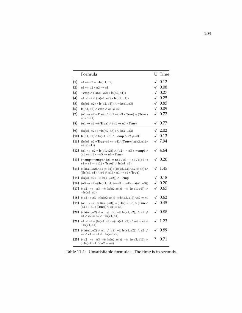
203
Formula U Time
(1) a1 7→ a2 ∧ ¬ls(a1, a2) X 0.12(2) a1 7→ a2 ∗ a2 7→ a1 X 0.08(3) ¬emp ∧ (ls(a1, a2) ∗ ls(a2, a1)) X 0.27(4) a1 6= a2 ∧ (ls(a1, a2) ∗ ls(a2, a1)) X 0.25(5) (ls(a1, a2) ∗ ls(a2, a3)) ∧ ¬ls(a1, a3) X 0.85(6) ls(a1, a2) ∧ emp ∧ a1 6= a2 X 0.09(7) (a1 7→ a2 ∗ True) ∧ (a2 7→ a3 ∗ True) ∧ (True ∗
a3 7→ a1)X 0.72
(8) (a1 7→ a2−~ True) ∧ (a1 7→ a2 ∗ True) X 0.77
(9) (ls(a1, a2) ∗ ¬ls(a2, a3)) ∧ ls(a1, a3) X 2.02(10) ls(a1, a2) ∧ ls(a1, a3) ∧ ¬emp ∧ a2 6= a3 X 0.13(11) (ls(a1, a2)∗True∗a3 7→ a4)∧(True∗(ls(a2, a1)∧
a2 6= a1))X 7.94
(12) (a1 7→ a2 ∗ ls(e1, e2)) ∧ (a2 7→ a3 ∗ ¬emp) ∧(a3 7→ a1 ∗ ¬a5 7→ a6 ∗ True)
X 4.64
(13) (¬emp∗¬emp)∧(a1 = nil∨a1 7→ e1∨((a1 7→e1 ∧ e1 = nil) ∗ True)) ∧ ls(a1, a2)
X 0.20
(14) ((ls(a1, a2)∧a1 6= a2)∗(ls(a2, a3)∧a2 6= a3))∧((ls(a4, a1) ∧ a4 6= a1) ∗ a1 7→ e1 ∗ True)
X 1.45
(15) (ls(a1, a2)−~ ls(a1, a2)) ∧ ¬emp X 0.18(16) (a3 7→ a4−~ls(a1, a4))∧(a3 = a4∨¬ls(a1, a3)) X 0.20(17) ((a2 7→ a3 −~ ls(a2, a4)) −~ ls(a1, a4)) ∧
¬ls(a1, a3)X 0.65
(18) ((a2 7→ a3−~ls(a2, a4))−~ls(a3, a1))∧a2 = a4 X 0.62(19) (a1 7→ a2−~ ls(a1, a3))∧ (¬ls(a2, a3)∨ (True∧
(a1 7→ e1 ∗ True)) ∨ a1 = a3)X 0.45
(20) ((ls(a1, a2) ∧ a1 6= a2) −~ ls(e1, e2)) ∧ e1 6=a1 ∧ e2 = a2 ∧ ¬ls(e1, a1)
X 0.88
(21) a1 6= a4∧ (ls(a1, a4)−~ ls(e1, e2))∧ a4 = e2∧¬ls(e1, a1)
X 1.23
(22) ((ls(a1, a2) ∧ a1 6= a2) −~ ls(e1, e2)) ∧ e2 6=a2 ∧ e1 = a1 ∧ ¬ls(a2, e2)
X 0.89
(23) ((a2 7→ a3 −~ ls(a2, a4)) −~ ls(a3, a1)) ∧(¬ls(a4, a1) ∨ a2 = a4)
? 0.71
Table 11.4: Unsatisfiable formulas. The time is in seconds.

204
Formula U Time
(1) ¬(a1 7→ a2) ∧ emp ∧ (a1 7→ a2 ∗ a3 7→ a4) X 0.83(2) a1 7→ a2 ∧ emp ∧ (¬(a1 7→ a2) ∗ a3 7→ a4) X 0.32(3) ¬(a1 7→ a2) ∧ emp ∧ (a1 7→ a2 ∗ ls(a3, a4)) X 0.62(4) ls(a1, a2) ∧ emp ∧ (¬ls(a1, a2) ∗ ls(a3, a4)) X 8.46(5) ls(a1, a2) ∧ emp ∧ (¬ls(a1, a2) ∗ ¬ls(a3, a4)) X 10.3
Table 11.5: Example instantiations of T1def= ¬a ∧ emp ∧ (a ∗ b), where a, b ∈ Literals. The time is
in seconds.
Though not shown in this section, I also evaluated our procedure on a set of satisfiable
formulas. The procedure reports a set of abstract models when given a satisfiable formula (see
Section 11.2.2).
We now answer Questions 1–3 posed at the beginning of this section using the three groups
of formulas.
Group 1 Results. The running time of our procedure on the formulas listed in Table 11.4 was
often on the order of one second. The TVLA startup and shutdown time for Group 1 was
10.9 seconds. The procedure was able to prove unsatisfiability for all formulas, except (23). I
believe that formulas (9)–(23) are beyond the scope of previously existing tools. Formulas (9)–(14)
demonstrate that we can handle formulas that describe overlapping data structures, including
conjunctions of separating conjunctions. Formulas (15)–(21) demonstrate that we can handle
formulas containing ls and septraction together.
Group 2 Results. The 64 formulas instantiated from the template T1def= ¬a ∧ emp ∧ (a ∗ b) took
between 0.0003 and 10.31 seconds to check, with a mean of 0.56 and a median of 0.03 seconds.
Our procedure was able to prove unsatisfiability for all 64 formulas. The TVLA startup and
shutdown time for Group 2 was 3.39 seconds. All instantiations of T1 that contain an occurrence
of the ls predicate are beyond the capabilities of existing tools. The formulas that took the most
time were (5) and (4) in Table 11.5. In both cases, a large amount of time was required because
of the presence of ¬ls, which is represented by 24 structures—a much larger number than is
needed for the other literals.

205
Formula U Time
(1) emp ∧ ls(a1, a2) ∧ (ls(a3, a4) ∗ (ls(a5, a6) −~(emp ∧ ¬ls(a1, a2))))
X 0.37
(2) emp ∧ ¬emp ∧ (ls(a3, a4) ∗ (¬(a5 7→ a6) −~(emp ∧ emp)))
X 0.17
(3) emp∧a1 7→ a2∧(a3 7→ a4∗(a5 7→ a6−~(emp∧¬(a1 7→ a2))))
X 0.49
(4) emp∧¬ls(a1, a2)∧ (¬ls(a3, a4)∗ (ls(a5, a6)−~(emp ∧ ls(a1, a2))))
X 3.97
(5) emp∧¬ls(a1, a2)∧(¬ls(a3, a4)∗(emp−~(emp∧ls(a1, a2))))
X 9.51
Table 11.6: Example instantiations ofT2def= emp∧a∧(b∗(c−~(emp∧¬a))), where a, b, c ∈ Literals.
The time is in seconds.
Group 3 Results. The 512 formulas instantiated from the template T2def= emp ∧ a ∧ (b ∗ (c−~
(emp ∧ ¬a))) took between 0.0001 and 9.51 seconds to check using our procedure, with a mean
of 0.12, and a median of 0.04 seconds. Our procedure was able to prove unsatisfiability for
all 512 formulas. The TVLA startup and shutdown time for Group 3 was 10.12 seconds. All
instantiations of T2 that contain an occurrence of ls are beyond the capabilities of existing tools.
11.5 Related Work
The literature related to reasoning about separation logic is vast, and I mention only a small
portion of it in this section. Decidability results related to first-order separation logic are discussed
in Calcagno et al. (2001); Brochenin et al. (2012). A fragment of separation logic for which it is
decidable to check validity of entailments was introduced by Berdine et al. (2004). The fragment
includes points-to and linked-list predicates, but no septraction, or negations of points-to or
linked-list predicates. More recent approaches deal with fragments of separation logic that are
incomparable to ours (Park et al., 2013; Lee and Park, 2014; Hou et al., 2014); in particular, none
of the latter papers handle linked lists. I based the experiments on formulas listed in Hou et
al.’s work on Boolean separation logic (Hou et al., 2014)—the only paper I found that listed
formulas outside the syntactic fragment defined by Berdine et al. I believe that our technique

206
represents the first important step in designing a verification system that uses a richer fragment
of separation logic.
Most approaches to separation-logic reasoning use a syntactic proof-theoretic procedure
(Berdine et al., 2004; Pérez and Rybalchenko, 2011). Two exceptions are the approaches of Cook
et al. (2011) and Enea et al. (2013), which use a more semantics-based approach: they represent
separation-logic formulas as graphs in a particular normal form, and then prove that one formula
entails another by finding a homomorphism between the corresponding graphs. Our approach
is also semantics-based, but has more of an algebraic flavor: our method performs a bottom-up
evaluation of a formula ϕ using a particular shape-analysis interpretation (Figure 11.4); if the
answer is the empty set of 3-valued structures, then ϕ is unsatisfiable.
To deal with overlaid data-structures, Enea et al. (2013) introduce the ∗w operator: the ∗w
operator specifies data structures that share sets of objects as long as they are built over disjoint
sets of fields. Their approach, however, does not handle conjunctions of separating conjunctions
or negations of the ls-predicate. Thus, Enea et al. (2013) cannot handle formulas (9)–(14) in
Table 11.4, even though these formulas do not contain septraction. Note that, for instance, the
logical conjunction in formula (9) cannot be replaced by the ∗w operator.
Piskac et al. (2013) present a decision procedure for a decidable fragment of separation logic
based on a reduction to a particular decidable first-order theory. Unlike our approach, the
approach in Piskac et al. (2013) does not handle septraction or negations below a separating
conjunction.
Many researchers pigeonhole TVLA (Lev-Ami and Sagiv, 2000) as a system exclusively
tailored for “shape analysis”. In fact, it is actually a metasystem for (i) defining a family of logical
structures 2-STRUCT[Voc], and (ii) defining canonical-abstraction domains whose elements
represent sets of 2-STRUCT[Voc]. The ITVLA (Jeannet et al., 2010, Section 8) variant of TVLA is
a different packaging of the classes that make up the TVLA implementation, and demonstrates
better that canonical abstraction is a general-purpose method for abstracting the structures that
are a logic’s domain of discourse.

207
To simplify matters, the separation-logic fragment addressed in this chapter does not allow
one to make assertions about numeric-valued variables and numeric-valued fields. Our approach
could be extended to support such capabilities using methods developed in work on abstract
interpretation that combines canonical abstraction with numeric abstractions (Gopan et al., 2004;
McCloskey et al., 2010).
11.6 Future Work
Ifϕ is satisfiable, then the procedure described in this chapter reports a set of abstract models—i.e.,
a value in the canonical-abstraction domain that overapproximates JϕK. As shown in Chapter 6
(using a variety of other techniques, and for a variety of other logics), a decision-procedure-like
method that is prepared to return such “residual” answers provides a way to generate sound
abstract transformers automatically. In particular, whenϕ specifies the transition relation between
the pre-state and post-state of a concrete transformer τ , a residuating decision procedure provides
a way to create a sound abstract transformer τ ] for τ , directly from a specification in logic of τ ’s
concrete semantics. Using our procedure, we now have a way to create abstract transformers
based on canonical-abstraction domains directly from a specification of the semantics of a
language’s concrete transformers, written in SL.
Although TVLA and separation logic have both been applied to the problem of analyzing
programs that manipulate linked data structures, there has been only rather limited crossover of
ideas between the two approaches. Our procedure is built on the connection between TVLA states
and SL statelets described in Section 11.1.3, which represents the first formal connection between
the two approaches. For this reason, the procedure should be of interest to both communities:
• For the TVLA community, the procedure illustrates a different and intriguing use for
canonical-abstraction domains. The domains that we use are tailored for the particular
formula, but, more importantly, provide an encoding that can be connected to the SL
semantics: see Equations (11.2) and (11.3) in Section 11.1.3, and the use of domain predicates
to express disjointness in Section 11.2.
208
• For the separation-logic community, the procedure shows how using TVLA and canonical-
abstraction domains leads to a model-theoretic approach to the decision problem for SL
that is capable of handling formulas that are beyond the capabilities of existing tools.
The question of whether or not the separation-logic fragment considered in this chapter
is decidable remains an open question. However, the eventual goal of this research direction
is to extend the approach to deal with richer fragments of separation logic. In particular, I
believe that our approach could be extended to perform unsatisfiability checking (and symbolic
abstraction) for undecidable fragments that contain both separating implication and acyclic
linked-list predicates.
11.7 Chapter Notes
The idea of building an SMA solver for separation logic using the abstract domain of TVLA shape
graphs seemed intuitive and straight forward at first. Devising the right abstraction predicates
for the TVLA abstract domain, and the correct integrity constraints for the coerce operation
turned out to be fiddly work. Further work in this direction would require automation of these
two tasks.
Jason Breck helped with the implementation of SMASLTOV, especially with the integration
of ITVLA with the latest implementation of TVLA.
Jason Breck and Thomas Reps came up with the name “SMASLTOV” for the SMA solver for
separation logic with only minor input from me.

209
Chapter 12
Property-Directed Symbolic
Abstraction
This chapter presents a framework for computing inductive invariants for a program that are
sufficient to prove that a given pre/post-condition holds, which I call the property-directed inductive-
invariant (PDII) framework. To understand the particular properties of the framework described
in this chapter I contrast it with the framework for computing best inductive A-invariants of
Chapter 7, which I will refer to as the BII framework:
1. The PDII framework computes an inductive invariant that might not be the best (or most
precise), but is sufficient to prove a given program property. The BII framework, in general,
aims to compute the best inductive A-invariant (in the given resource/time constraints).
2. In case the program does not satisfy the given property, the PDII framework reports a
concrete counter-example to the property. The BII framework is agnostic to the particular
property to be proved.
3. The PDII framework is applicable to the abstract domain of full predicate abstraction; the
BII framework can be instantiated with a larger class of abstract domains, which includes
full predicate abstraction.
210
The advantages of the PDII method described in this chapter are two-fold:
1. The PDII framework obtains the same precision as the best abstract transformer for full
predicate abstraction, without ever constructing the transformers explicitly.
2. The PDII framework is relatively complete with respect to the given abstraction. That is, the
analysis is guaranteed to terminate and either
a) verifies the given property,
b) generates a concrete counterexample to the given property, or
c) reports that the abstract domain is not expressive enough to establish the proof.
Note that outcome c) is a much stronger guarantee than what other approaches provide in
such cases when they neither succeed nor give a concrete counterexample.
The PDII framework is based on the IC3 algorithm (Bradley, 2011), which is also referred
to as property-directed reachability (PDR). The PDR algorithm was chosen for the following two
reasons:
• The PDR algorithm has been shown to work extremely well in other domains, such as
hardware verification (Bradley, 2011; Eén et al., 2011). Subsequently, it was generalized to
software model checking for program models that use linear real arithmetic (Hoder and
Bjørner, 2012) and linear rational arithmetic (Cimatti and Griggio, 2012).
• The PDR algorithm maintains a “frame” structure, which can be used to build a trace
formula; if the formula is satisfiable, the model can be presented to the user as a concrete
counterexample (outcome b)).
In this chapter I describe how to integrate PDR with full predicate abstraction, and cast PDR
as a framework that is parameterized on
• the logic L in which the semantics of program statements are expressed, and

211
Algorithm 23: PDIIA(Init, ρ,Bad)1 R[−1]← false2 R[0]← true3 N ← 04 while true do5 if there exists 0 ≤ i < Nsuch that R[i] = R[i+ 1] then6 return valid7 (r,A)← CheckA(Bad, R[N ])8 if r = unsat then9 N ← N + 1
10 R[N ]← true11 else12 reduceA(N,A)
• the finite set of predicates that define the abstract domain A in which invariants can be
expressed. An element of A is an arbitrary Boolean combination of the predicates.
The PDII framework has been instantiated to prove shape properties of programs manip-
ulating singly linked lists. This instantiation represents the first algorithm for shape analysis
that either (i) succeeds, (ii) returns a concrete counterexample, or (iii) returns an abstract trace
showing that the abstraction in use is not capable of proving the property in question. Details of
the instantiation to shape analysis and the experimental evaluation can be found in Itzhaky et al.
(2014).
The contribution of this chapter is:
• The PDII framework, based on the PDR algorithm, for finding an inductive invariant in a
certain logic fragment (abstract domain) that allows one to prove that a given pre-/post-
condition holds or find a concrete counter-example to the property, or, in the case of a
negative result, the information that there is no inductive invariant expressible in the
abstract domain (Section 12.1).

212
Algorithm 24: reduceA(j, A)1 (r,A1)← CheckA(Init, A)2 if r = sat then3 σ ← Model(Init ∧ ρN−j ∧ (Bad)′×(N−j))4 if σ is None then5 error “abstraction failure”6 else7 error “concrete counterexample(σ)”8 while true do9 (r,A2)←
10 CheckA((Init)′ ∨ (R[j − 1] ∧ ρ), (A)′)11 if r = unsat then12 break13 else14 reduceA(j − 1, A2)15 for i = 0 . . . j do16 R[i]← R[i] ∧ (¬A1 ∨ ¬A2)
12.1 The Property-Directed Inductive Invariant (PDII) Algorithm
In this section, I present the PDII framework, which is an adaptation of the PDR algorithm that
uses predicate abstraction. In this chapter, by predicate abstraction I mean the technique that
performs verification using a given fixed set of abstraction predicates (Flanagan and Qadeer,
2002), and not techniques that incorporate automatic refinement of the abstraction predicates;
e.g., CEGAR. The PDII algorithm shown in Algorithm 23 is parameterized by a given finite set
of predicates P expressed in a logic L. The requirements on the logic L are:
R1 L is decidable (for satisfiability).
R2 The transition relation for each statement of the programming language can be expressed
as a two-vocabulary L formula.
Then for a particular program, we are given:
• A finite set of predicates P = {pi ∈ L}, 1 ≤ i ≤ n.
• The transition relation of the system as a two-vocabulary formula ρ ∈ L.

213
• The initial condition of the system, Init ∈ L.
• The formula specifying the set of bad states, Bad ∈ L.
Let A be the full predicate-abstraction domain over the predicates P . That is, each element
A ∈ A is an arbitrary Boolean combination of the predicates P . A ∈ A is inductive with respect
to Init and ρ if and only if Init⇒A and A ∧ ρ⇒(A)′. (ϕ)′ renames the vocabulary of constant
symbols and relation symbols occurring in ϕ from {c, . . . , r, . . .} to {c′, . . . , r′, . . .}. ϕ is (ϕ)′
stripped of primes.
If the logic L is propositional logic, then Algorithm 23 is an instance of IC3 (Bradley, 2011).
This presentation is a simplification of more advanced variants (Bradley, 2011; Eén et al., 2011;
Hoder and Bjørner, 2012). For instance, the presentation omits inductive generalization, although
the implementation of the framework does implement inductive generalization (Itzhaky et al.,
2014). Furthermore, this simplified presentation brings out the fact that the PDR algorithm is
really an analysis framework that is parameterized on the set of abstraction predicates P .
The algorithm employs an unbounded arrayR, where each frame R[i] ∈ A over-approximates
the set of concrete states after executing the loop at most i times. The algorithm maintains an
integer N , called the frame counter, such that the following invariants hold for all 0 ≤ i < N :
1. Init is a subset of all R[i], i.e., Init⇒R[i].
2. The safety requirements are satisfied, i.e., R[i]⇒¬Bad.
3. Each of the R[i+ 1] includes the states in R[i], i.e., R[i]⇒R[i+ 1].
4. The successors of R[i] are included in R[i+ 1], i.e., for all σ, σ′ if σ |= R[i] and 〈σ, σ′〉 |= ρ,
then σ′ |= R[i+ 1].
Some terminology used in the PDII algorithm:
• Model(ϕ) returns a model σ satisfying ϕ if it exists, and None if it doesn’t.
• The abstraction of a model σ, denoted by βA(σ), is the cube of predicates from P that hold
in σ: βA(σ) =∧{p | σ |= p, p ∈ P} ∧
∧{¬q | σ |= ¬q, q ∈ P}.
214
• Let ϕ ∈ L be a formula, and let A ∈ A be a value in the unprimed or primed vocabulary.
CheckA(ϕ,A) returns a pair (r,A1) such that
– if ϕ ∧A is satisfiable, then r = sat and A1 is the abstraction of a concrete state in the
unprimed vocabulary. That is, if the given A is in the unprimed vocabulary, then
βA(σ) for some σ |= ϕ ∧A; else if A is in the primed vocabulary, then A1 = βA(σ) for
some (σ, σ′) |= ϕ ∧A.
– if ϕ ∧A is unsatisfiable, then r = unsat, and A1 is a predicate such that A⇒A1 and
ϕ ∧ A1 is unsatisfiable. The vocabulary of A1 is the same as that of A. If A is in the
primed vocabulary (as in line 10 of Algorithm 24), CheckA drops the primes from A1
before returning the value.
A valid choice for A1 in the unsatisfiable case would be A1 = A (and indeed the algorithm
would still be correct), but ideally A1 should be the weakest such predicate. For instance,
CheckA(false, A) should return (unsat, true). In practice, when ϕ ∧A is unsatisfiable, the
A1 returned is an unsat core of ϕ ∧A constructed exclusively from conjuncts of A. Such an
unsat core is a Boolean combination of predicates in P , and thus is an element of A.
I now give a more detailed explanation of Algorithm 23. Each R[i], i ≥ 0 is initialized to
true (lines 2 and 10), and R[−1] is false. N is initialized to 0 (line 3). At line 5, the algorithm
checks whether R[i] = R[i+ 1] for some 0 ≤ i < N . If true, then an inductive invariant proving
unreachability of Bad has been found, and the algorithm returns valid (line 6).
At line 7, the algorithm checks whetherR[N ]∧Bad is satisfiable. If it is unsatisfiable, it means
that R[N ] excludes the states described by Bad, and the frame counter N is incremented (line 9).
Otherwise, A ∈ A represents an abstract state that satisfies R[N ] ∧ Bad. PDII then attempts to
reduce R[N ] to try and exclude this abstract counterexample by calling reduceA(N,A) (line 12).
The reduce algorithm (Algorithm 24) takes as input an integer j, 0 ≤ j ≤ N , and an abstract
stateA ∈ A such that there is a path starting fromA of lengthN−j that reaches Bad. Algorithm 24
tries to strengthen R[j] so as to exclude A. At line 1, reduce first checks whether Init ∧ A is

215
satisfiable. If it is satisfiable, then there is an abstract trace of length N − j from Init to Bad, using
the transition relation ρ. The call to Model at line 3 checks whether there exists a concrete model
corresponding to the abstract counterexample. ρk denotes k unfoldings of the transition relation
ρ; ρ0 is true. (Bad)′×k denotes k applications of the renaming operation (·)′ to Bad. If no such
concrete model is found, then the abstraction was not precise enough to prove the required
property (line 5); otherwise, a concrete counterexample to the property is returned (line 7).
Now consider the case when Init∧A is unsatisfiable on line 1. A1 ∈ A returned by the call to
CheckA is such that Init ∧A1 is unsatisfiable; that is, Init⇒¬A1.
The while-loop on lines 8–14 checks whether the (N − j)-length path to Bad can be extended
backward to an (N − j + 1)-length path. In particular, it checks whether R[j − 1] ∧ ρ ∧ (A)′ is
satisfiable. If it is satisfiable, then the algorithm calls reduce recursively on j − 1 and A2 (line 14).
If no such backward extension is possible, the algorithm exits the while loop (line 12). Note that
if j = 0, CheckA(R[j − 1] ∧ ρ,A) returns (unsat, true), because R[−1] is set to false.
The conjunction of (¬A1 ∨ ¬A2) to R[i], 0 ≤ i ≤ j, in the loop on lines 15–16 eliminates
abstract counterexample A while preserving the required invariants on R. In particular, the
invariant Init⇒R[i] is maintained because Init⇒¬A1, and hence Init⇒(R[i] ∧ (¬A1 ∨ ¬A2)).
Furthermore, A2 is the abstract state from which there is a (spurious) path of length N − j to Bad.
By the properties of CheckA, ¬A1 and ¬A2 are each disjoint from A, and hence (¬A1 ∨ ¬A2) is
also disjoint from A. Thus, conjoining (¬A1 ∨ ¬A2) to R[i], 0 ≤ i ≤ j eliminates the spurious
abstract counterexampleA. Lastly, the invariantR[i]⇒R[i+1] is preserved because (¬A1∨¬A2)
is conjoined to all R[i], 0 ≤ i ≤ j, and not just R[j].
Formally, the output of PDIIA(Init, ρ,Bad) is captured by the following theorem. The proof
of Theorem 12.1 is based on the observation that, when “abstraction failure” is reported by
reduceA(j, A), the set of models σi |= R[i] (j ≤ i < N ) represents an abstract error trace.
Theorem 12.1. Given (i) the set of abstraction predicates P = {pi ∈ L}, 1 ≤ i ≤ n where L is a
decidable logic, and the full predicate-abstraction domain A over P , (ii) the initial condition Init ∈ L,
(iii) a transition relation ρ expressed as a two-vocabulary formula in L, and (iv) a formula Bad ∈ L
216
specifying the set of bad states, PDIIA(Init, ρ,Bad) terminates, and reports either
1. valid if there exists A ∈ A s.t. (i) Init⇒A, (ii) A is inductive, and (iii) A⇒¬Bad,
2. a concrete counterexample trace, which reaches a state satisfying Bad, or
3. an abstract trace, if the inductive invariant required to prove the property cannot be expressed as an
element of A.
Proof. The first two cases are trivial: if PDIIA terminates returning some R[j], j < N , then
Init⇒R[j] by virtue of Init⇒R[0] and R[i]⇒R[i+ 1] for every i < N , and R[j]⇒¬Bad or the
check at line 7 would have failed. Also, R[j − 1] ≡ R[j] so R[j] is inductive.
If PDIIA returns a set of concrete states, then they have to be a concrete counterexample trace,
because they are a model of Init ∧ ρN−j ∧ (Bad)′×(N−j) (line 3 of reduceA).
For the third case, we show that if the check on the first line of “reduce” is “sat”, then there
exists a chain of concrete states, σj σj+1 · · · σN , such that σj |= Init, σN |= Bad, and for any
j ≤ i < N there exist two concrete states σ, σ′ satisfying:
• σ ∈ γ(βA(σi))
• σ′ ∈ γ(βA(σi+1))
• 〈σ, σ′〉 |= ρ
The key point is that, because the given abstraction can never distinguish any two states in
γ(βA(σi)), the chain σj σj+1 · · ·σN cannot be excluded by the abstract domainA, no matter what
Boolean combination of the predicates ofP is used. Moreover, the chainβA(σj)βA(σj+1) · · · βA(σN )
is an abstract trace that leads from an initial state to an error state.
Notice that the chain above may not be a concrete trace, there can be “breaks” between
adjacent σis, within the same abstract element.
Construction of (σi)i=j...N : Follow the chain of recursive calls to “reduce” with index values
N down to j. The parameter A is always a cube of the form βA(σ); take one σ |= A for each
217
call, forming a series that we denote by σj , σj+1, etc. We show that this series satisfies the above
properties: At each call except the innermost, “reduce” made a recursive call at line 7, which
means that R[j − 1] ∧ ρ ∧ (A)′ was satisfiable; the returned cube A2 becomes βA(σj−1). Let
〈σ, σ′〉 |= R[j − 1] ∧ ρ ∧ (A)′, then σ |= A2 = βA(σj−1); σ′ |= A = βA(σj); and 〈σ, σ′〉 |= ρ as
required.
12.2 Chapter Notes
The research presented in this chapter was done in collaboration with Shachar Itzhaky, Niko-
laj Bjorner, Mooly Sagiv, and Thomas Reps. In this chapter, I have presented my primary
contribution—that is, the formulation of the generalized PDII framework (Algorithms 23 and 24).
The implementation of this generalized PDII framework, its instantiation to shape analysis of
programs manipulating singly linked lists, and the experimental evaluation of this instantiation
was mainly carried out by Shachar Itzhaky and Nikolaj Bjorner. Because I did not play a major
role in those aspects of the research, I chose to omit them from the thesis.
Key to instantiating the PDII framework for shape analysis of programs manipulating singly
linked lists was the recent development of the AFR and EAR logics for expressing properties of
linked lists (Itzhaky et al., 2013). AFR is used to define abstraction predicates, and EAR is used to
express the language semantics. AFR is a decidable, alternation-free fragment of first-order logic
with transitive closure (FOTC). When applied to list-manipulation programs, atomic formulas of
AFR can denote reachability relations between memory locations pointed to by pointer variables,
where reachability corresponds to repeated dereferences of next or prev fields. One advantage of
AFR is that it does not require any special-purpose reasoning machinery: an AFR formula can be
converted to a formula in “effectively propositional” logic, which can be reduced to SAT solving.
That is, in contrast to much previous work on shape analysis, this PDR-based method makes
use of a general purpose SMT solver, Z3 (de Moura and Bjørner, 2008) (rather than specialized
tools developed for reasoning about linked data structures, e.g., (Sagiv et al., 2002; Distefano

218
et al., 2006; Berdine et al., 2007; Garg et al., 2013)). The reader is encouraged to read Itzhaky et al.
(2014) to learn more about this application of the PDII framework to shape analysis.
219
Chapter 13
Conclusion
This chapter summarizes the results developed during my dissertation research, and presents
my contributions to advancing the field.
The thesis explored the use of abstraction in two areas of automated reasoning: verification
of programs, and decision procedures for logics. Chapter 1 laid the groundwork for the thesis
by viewing these two research areas through the lens of abstraction. Many of the applications
discussed in the thesis dealt with verification of machine code, a burgeoning subfield of program
verification (Chapter 2).
The unifying theme behind the thesis is the concept of symbolic abstraction (Reps et al., 2004):
Given a formula ϕ in logic L and an abstract domain A, the symbolic abstraction of
ϕ, denoted by α(ϕ), is the strongest consequence of ϕ expressible in A.
Symbolic abstraction bridges the gap between abstraction and logic, and many of the operations
required by an abstract interpreter can be implemented using symbolic abstraction (Section 3.2.3).
Furthermore, this thesis showed how the concept of symbolic abstraction brings forth the
connection between abstract interpretation (Cousot and Cousot, 1977) and decision procedures
for logics.
Instead of summarizing each individual chapter, I chose to present the results for the three
research threads discussed in this thesis: abstract interpretation (Section 13.1), machine-code

220
verification (Section 13.2), and decision procedures (Section 13.3). Note that because some of the
chapters touch on more than one research thread, there is some repetition of text between the
sections in this chapter.
13.1 Abstract Interpretation
The contributions of the thesis in the field of abstract interpretation are:
• New algorithms for performing symbolic abstraction (Chapters 5 and 6).
• New algorithms for computing inductive invariants for programs (Chapters 7 and 12).
• A new abstract domain for bit-vector inequalities implemented using symbolic abstraction
(Chapter 8).
Chapter 4 reviewed two prior algorithms for performing symbolic abstraction:
• The RSY algorithm: a framework for computing α that applies to any logic and abstract
domain that satisfies certain conditions (Reps et al., 2004).
• The KS algorithm: an algorithm for computing α that applies to QFBV logic and the domain
E2w of affine equalities (Elder et al., 2011).
Both algorithms compute α(ϕ) via successive approximation from “below”, computing a se-
quence of successively “larger” approximations to the set of states described by ϕ. Section 4.3
presented an empirical comparison of the RSY and KS algorithms that showed that the KS
algorithm was ten times faster than the RSY algorithm. The main insight from this experiment
was that, while the KS algorithm invokes the decision procedure more often, each of the calls to
the decision procedure is significantly less expensive, compared to that in the RSY algorithm.
221
In Chapter 5, I used the insights gained from the algorithms presented in Chapter 4 to design
a new framework for symbolic abstraction that
• is parametric and is applicable to any abstract domain that satisfies certain conditions
(similar to the RSY algorithm)
• uses a successive-approximation algorithm that is parsimonious in its use of the decision
procedure (similar to the KS algorithm)
• is bilateral; that is, it maintains both an under-approximation and a (non-trivial) over-
approximation of the desired answer, and hence is resilient to timeouts: the procedure
can return the over-approximation if it is stopped at any point (unlike the RSY and KS
algorithms).
In contrast, neither the RSY algorithm nor KS algorithm is resilient to timeouts. A decision-
procedure query—or the cumulative time for the algorithm—might take too long, in which case
the only safe answer that can be returned is >.
The key insight behind the new bilateral framework for symbolic abstraction, denoted by αl,
was the notion of an abstract consequence (Definition 5.1).
Chapter 6 presented an algorithm for symbolic abstraction that is based on much different
principles from the RSY, KS, and bilateral algorithms. The latter frameworks use an inductive-
learning approach to learn from examples. In contrast, the symbolic-abstraction framework dis-
cussed in Chapter 6 uses a deductive approach, and is based on the following two insights:
• Each of the key components in Stålmarck’s method (Sheeran and Stålmarck, 2000), an
algorithm for satisfiability checking of propositional formulas, can be explained in terms
of concepts from the field of abstract interpretation. In particular, I showed that Stål-
marck’s method can be viewed as a general framework, which I call Stålmarck[A], that is
parameterized by an abstract domain A and operations on A.

222
• When viewed through the lens of abstraction, there is a connection between this generalized
Stålmarck’s method and symbolic abstraction. In particular, to check whether a formula ϕ
is unsatisfiable, Stålmarck[A] computes α(ϕ).
This new algorithm for symbolic abstraction based on Stålmarck’s method approaches its result
from “above”, and is denoted by α↓. Because the method approaches its result from “above”,
if the computation takes too much time, it can be stopped to yield a safe result—i.e., an over-
approximation to the best abstract operation—at any stage, similar to the bilateral framework
(Chapter 5). Section 6.4.1 presented an empirical comparison between the Stålmarck-based
algorithm (α↓), and the bilateral algorithm (α↓), which showed that α↓ is faster and more precise
compared to αl.
Chapters 7 and 12 present two different algorithms for computing inductive invariants for a
program. Chapter 7 presents a framework for computing best inductive A-invariants, which is
based on the following insights:
• The BII problem reduces to the problem of applying Post.
• The problem of applying Post reduces to the problem of symbolic abstraction.
This work provided insight on fundamental limits in abstract interpretation. Furthermore, the
BII algorithm presented is also practical: Santini is an invariant-generation tool based on the
principles of symbolic abstraction. The performance of the Corral model checker (Lal et al., 2012)
improved when using invariants supplied by Santini, compared to using invariants supplied by
Houdini (Flanagan and Leino, 2001); see (Thakur et al., 2013, Section 5). This experiment shows
that symbolic abstraction provides a powerful tool that can be used to implement automatically
a correct and precise invariant generator that uses an expressive abstract domain.
Chapter 12 presents a framework for computing inductive invariants for a program that are
sufficient to prove that a given pre/post-condition holds, which I called the property-directed
inductive-invariant (PDII) framework. The PDII framework computes an inductive invariant that
might not be the best (or most precise), but is sufficient to prove a given program property. In

223
case the program does not satisfy the given property, the PDII framework reports a concrete
counter-example to the property. The PDII framework is applicable to the abstract domain of
full predicate abstraction. The advantages of the PDII method are two-fold:
1. The PDII framework obtains the same precision as the best abstract transformer for full
predicate abstraction, without ever constructing the transformers explicitly.
2. The PDII framework is relatively complete with respect to the given abstraction. That is, the
analysis is guaranteed to terminate and either
a) verifies the given property,
b) generates a concrete counterexample to the given property, or
c) reports that the abstract domain is not expressive enough to establish the proof.
Note that outcome c) is a much stronger guarantee than what other approaches provide in
such cases when they neither succeed nor give a concrete counterexample.
The PDII framework is based on the IC3 algorithm (Bradley, 2011) (sometimes called property-
directed reachability (PDR)). An instantiation of the PDII framework to prove shape properties of
programs manipulating singly linked lists can be found in Itzhaky et al. (2014).
Chapter 8 presents the design and implementation of a new abstract domain for bit-vector
inequalities, called the BVI domain. The key insights behind the design of the BVI domain
were:
• We extend the standard vocabulary of an abstract domain with view expressions, which are
w-bit terms expressed in some logic L. Thus, view expressions are capable of holding onto
richer constraints about the program state than the unenriched abstract domain alone.
• We construct the BVI domain as a reduced product between the bit-vector affine-equality
domain E2w and the bit-vector interval domain I2w .
• We use symbolic abstraction to implement precise versions of the abstract-domain opera-
tions for BVI.

224
13.2 Machine-Code Verification
Chapter 2 discussed the unique challenges and opportunities involved in analyzing machine
code. The contributions of the thesis in the field of machine-code analysis and verification are:
• New techniques for computing abstract transformers used to perform machine-code analy-
sis (Chapters 5 and 6).
• A new abstract domain for bit-vector inequalities (Chapter 8).
• A new model-checking algorithm for stripped machine-code, called MCVETO (Chapter 9).
The use of symbolic abstraction greatly reduces the burden on the analysis writer when
implementing abstract operations required for performing analysis. This benefit is especially
helpful when implementing machine-code analyses, because most machine-code instructions
involve bit-wise operations. Section 1.1 illustrated how existing approaches to computing abstract
transformers based on quantifier elimination are not applicable to machine-code analysis. On the
other hand, computing abstract transformers based on operator-by-operator reinterpretation can
be tedious, error-prone, and not precise (Section 3.1.2). The experiments described in Sections 5.5
and 6.4.1 illustrate how the new algorithms for symbolic abstraction can be used to compute
invariants for x86 machine code.
Chapter 8 described how symbolic abstraction enabled us to define a new abstract domain,
called the Bit-Vector Inequality (BVI) domain, that addresses the following challenges: (1) identify-
ing affine-inequality invariants while handling overflow in arithmetic operations over bit-vector
data-types, and (2) holding onto invariants about values in memory during machine-code analy-
sis. The experiments in Section 9.4 showed that an analysis based on the BVI domain is capable
of proving programs correct that could not be proved correct using existing abstract domains.
Chapter 9 described a new model-checking algorithm for stripped machine-code, called
MCVETO (Machine-Code VErification TOol). MCVETO is able to detect and explore “deviant
behavior” in machine code. An example of such deviant behavior is when the program over-
writes the return address stored on the stack frame. Moreover, MCVETO is capable of verifying

225
(or detecting flaws in) self-modifying code (SMC). To the best of my knowledge, MCVETO is the
first model checker to handle SMC. The key insights behind the design of MCVETO are:
• MCVETO adapts directed proof generation (DPG) (Gulavani et al., 2006) for model checking
stripped machine code.
• MCVETO uses trace-based generalization to build and refine an abstraction of the program’s
state space entirely on-the-fly. Trace-based generalization enables MCVETO to handle
instruction aliasing and SMC.
• MCVETO uses speculative trace refinement to identify candidate invariants that can speed up
the convergence of DPG.
The experiments in Section 9.4 showed that MCVETO is able to prove properties of small, but
complicated, programs. The experiments also showed how candidate invariants obtained using
the BVI domain can help speed up the convergence of DPG.
13.3 Decision Procedures
This thesis introduced a new approach for designing and implementing decision procedures
based on the use of abstraction. This abstraction-centric view of decision procedures is called
Satisfiability Modulo Abstraction (SMA). Abstraction provides a new language for the description
of decision procedures, and lead to new insights and new ways of thinking about decision
procedures. Furthermore, the SMA approach is able to reuse abstract-interpretation machinery
to implement decision procedures.

226
The contributions of the thesis in the field of decision procedures are:
• An SMA solver based on a generalization of Stålmarck’s method (Sheeran and Stålmarck,
2000) (Chapter 6).
• A new distributed SAT solver, called DiSSolve (Chapter 10).
• An SMA solver for a new fragment of separation logic (Chapter 11).
Chapter 6 presented a new SMA solver that is based on the following two insights:
• Each of the key components in Stålmarck’s method (Sheeran and Stålmarck, 2000), an
algorithm for satisfiability checking of propositional formulas, can be explained in terms
of concepts from the field of abstract interpretation. In particular, I showed that Stål-
marck’s method can be viewed as a general framework, which I call Stålmarck[A], that is
parameterized on an abstract domain A and operations on A.
• When viewed through the lens of abstraction, Stålmarck’s method can be lifted from
propositional logic to richer logics, such as LRA: to obtain a method for richer logics,
instantiate the parameterized version of Stålmarck’s method with richer abstract domains,
such as the polyhedral domain (Cousot and Halbwachs, 1978).
This abstraction-based approach provides new insights into the working Stålmarck’s method. In
particular, at each step, Stålmarck[A] holds some A ∈ A; each of the proof rules employed in
Stålmarck’s method improves A by finding a semantic reduction (Cousot and Cousot, 1979) of A
with respect to ϕ. Furthermore, Section 6.4.2 shows how this generalized Stålmarck’s method
outperforms an existing SMT solver on a family of LRA formulas.
Chapter 10 described a new distributed SAT solver, called DiSSolve, which uses a new proof
rule that combines concepts from Stålmarck’s method with those found in modern DPLL/CDCL
solvers:
1. DiSSolve partitions the search space using k variables in the same fashion that the Dilemma
Rule partitions the search space in Stålmarck’s method.

227
2. Each of the 2k branches can be solved concurrently with the help of a sequential DPLL/CDCL
solver, similar to what is done in the divide-and-conquer approach to parallel SAT solvers.
3. The DPLL/CDCL solver assigned to a branch is allotted a finite amount of time, after
which the DPLL/CDCL solver returns a set of learned clauses. Such a branch-and-merge
approach does not have to as careful about load balancing, unlike the divide-and-conquer
approach.
4. DiSSolve performs a union of the information from all the branches, instead of an inter-
section as done in Stålmarck’s method. Performing a union of clauses is more effective
at pruning the search space compared to computing an intersection: with intersection
only common information learned by every process can be used to prune the search space,
while with union, all of the information learned by each process can be used to prune the
search space. In abstract-interpretation terms, DiSSolve combines the information from
the branches using a meet (u), while the Dilemma Rule in Stålmarck’s method combines
the information using a join (t).
Section 10.2 illustrated the effectiveness of DiSSolve when deployed on a multi-core machine,
and on a cloud-computing platform. Section 10.3 described a natural extension of DiSSolve
from SAT to SMT, and also presented the algorithm using abstract-interpretation terminology.
Chapter 11 described an SMA solver for checking the unsatisfiability of formulas in a new
fragment of separation logic. Separation logic (Reynolds, 2002) is an expressive logic for reasoning
about heap-allocated data structures in programs. The SMA solver uses the abstract domain of
shape graphs—implemented in TVLA (Sagiv et al., 2002)—to represent a set of heap structures.
The SMA solver performs a bottom-up evaluation of the given formula ϕ to compute an abstract
value that over-approximates the set of satisfying models of ϕ. If the over-approximation is the
empty set of shape graphs, then ϕ is unsatisfiable. If ϕ is satisfiable, then the procedure reports
a set of abstract models.
The SMA solver for separation logic is implemented in a tool called SMASLTOV (Satisfiability
Modulo Abstraction for Separation Logic ThrOugh Valuation), which is available at https://www.

228
github.com/smasltov-team/SMASLTOV. Section 11.4 described an evaluation of SMASLTOV on
a set of formulas taken from the literature. To the best of my knowledge, SMASLTOV is able to
establish the unsatisfiability of formulas that cannot be handled by previous approaches.
The wind blew southward, through knotted forests, over shimmering plains and
toward land unexplored. This wind, it was not the ending. There are no endings,
and never will be endings, to the turning of the Wheel of Time.
But it was an ending.— Robert Jordan and Brandon Sanderson, A Memory of Light
229
References
Abramson, Darren, and Lee Pike. 2011. When formal systems kill: Computer ethics and formal
methods. APA Newsletter on Philosophy and Computers.
Allauzen, C., M. Riley, J. Schalkwyk, W. Skut, and M. Mohri. 2007. OpenFst: A general and
efficient weighted finite-state transducer library. In Conference on implementation and application
of automata (CIAA).
Alur, R., and P. Madhusudan. 2009. Adding nesting structure to words. Journal of ACM (JACM)
56(3).
Alur, Rajeev, Rastislav Bodik, Garvit Juniwal, Milo MK Martin, Mukund Raghothaman, Sanjit A
Seshia, Rishabh Singh, Armando Solar-Lezama, Emina Torlak, and Abhishek Udupa. 2013.
Syntax-guided synthesis. In Formal methods in computer-aided design (FMCAD).
AMD. 2012. AMD cpu bug update – AMD confirms! http://article.gmane.org/gmane.os.
dragonfly-bsd.kernel/14518.
Angluin, Dana. 1987. Learning regular sets from queries and counterexamples. Information and
computation 75(2):87–106.
Arnold, G., R. Manevich, M. Sagiv, and R. Shaham. 2006. Combining shape analyses by
intersecting abstractions. In Verification, model checking, and abstract interpretation (VMCAI).
230
Audemard, G., B. Hoessen, S. Jabbour, J. Lagniez, and C. Piette. 2012. Revisiting clause exchange
in parallel SAT solving. In International conference on theory and applications of satisfiability testing
(SAT).
Audemard, Gilles, and Laurent Simon. 2009. Predicting learnt clauses quality in modern SAT
solvers. In International joint conference on artificial intelligence (IJCAI), 399–404.
Bagnara, R., P. M. Hill, and E. Zaffanella. 2008. The Parma Polyhedra Library: Toward a complete
set of numerical abstractions for the analysis and verification of hardware and software systems.
Science of Computer Programming (SCP) 72(1–2):3–21.
Balakrishnan, G., and T. Reps. 2008. Analyzing stripped device-driver executables. In Tools and
algorithms for the construction and analysis of systems (TACAS).
———. 2010. WYSINWYX: What You See Is Not What You eXecute. ACM Transactions on
Programming Languages and Systems (TOPLAS) 32(6).
Balakrishnan, G., T. Reps, N. Kidd, A. Lal, J. Lim, D. Melski, R. Gruian, S. Yong, C.-H. Chen,
and T. Teitelbaum. 2005. Model checking x86 executables with CodeSurfer/x86 and WPDS++.
In Computer aided verification (CAV).
Balakrishnan, G., T. Reps, D. Melski, and T. Teitelbaum. 2007. WYSINWYX: What You See Is
Not What You eXecute. In Verified software: Theories, tools, experiments (VSTTE).
Ball, T., A. Podelski, and S.K. Rajamani. 2001. Boolean and Cartesian abstraction for model
checking C programs. In Tools and algorithms for the construction and analysis of systems (TACAS),
268–283.
Ball, T., and S.K. Rajamani. 2000. Bebop: A symbolic model checker for Boolean programs. In
SPIN model checking and software verification.
———. 2001. The SLAM toolkit. In Computer aided verification (CAV).

231
Ball, Thomas, Byron Cook, Vladimir Levin, and Sriram K Rajamani. 2004. Slam and static driver
verifier: Technology transfer of formal methods inside microsoft. In Integrated formal methods.
Barrett, Clark, Roberto Sebastiani, Sanjit A. Seshia, and Cesare Tinelli. 2009. Satisfiability
modulo theories. In Handbook of satisfiability, ed. Armin Biere, Marijn Heule, Hans van Maaren,
and Toby Walsh, vol. 185 of Frontiers in Artificial Intelligence and Applications, 825–886. IOS Press.
Barrett, E., and A. King. 2010. Range and set abstraction using SAT. Electronic Notes in Theoretical
Computer Science (ENTCS).
Beckman, N.E., A.V. Nori, S.K. Rajamani, and R.J. Simmons. 2008. Proofs from tests. In
International symposium on software testing and analysis (ISSTA).
Berdine, J., C. Calcagno, B. Cook, D. Distefano, P.W. O’Hearn, T. Wies, and H. Yang. 2007. Shape
analysis for composite data structures. In Computer aided verification (CAV).
Berdine, J., C. Calcagno, and P. O’Hearn. 2004. A decidable fragment of separation logic. In
Foundations of software technology and theoretical computer science (FSTTCS).
———. 2005. Smallfoot: modular automatic assertion checking with separation logic. In Formal
methods for components and objects (FMCO).
Bessey, Al, Ken Block, Ben Chelf, Andy Chou, Bryan Fulton, Seth Hallem, Charles Henri-Gros,
Asya Kamsky, Scott McPeak, and Dawson Engler. 2010. A few billion lines of code later: using
static analysis to find bugs in the real world. Communications of the ACM (CACM) 53(2):66–75.
Beyer, D., T.A. Henzinger, R. Majumdar, and A. Rybalchenko. 2007. Path invariants. In ACM
SIGPLAN conference on programming language design and implementation (PLDI).
Biere, Armin. 2008. PicoSAT essentials. Journal of Satisfiability, Boolean Modeling and Computation
(JSAT) 4(2-4):75–97.
———. 2009. Bounded model checking. In Handbook of satisfiability, ed. Armin Biere, Marijn
Heule, Hans van Maaren, and Toby Walsh, vol. 185 of Frontiers in Artificial Intelligence and
Applications, 457–482. IOS Press.
232
Bjesse, Per, and Koen Claessen. 2000. SAT-based verification without state space traversal. In
Formal methods in computer-aided design (FMCAD).
Björk, M. 2009. First order Stålmarck. Journal of Automated Reasoning (JAR) 42(1):99–122.
Bjørner, N., and L. de Moura. 2008. Accelerated lemma learning using joins–DPLL(t). In Logic
for programming, artificial intelligence, and reasoning (LPAR).
Bloch, Joshua. 2014. Extra, extra - read all about it: Nearly all binary
searches and mergesorts are broken. googleresearch.blogspot.com/2006/06/
extra-extra-read-all-about-it-nearly.html.
Bloom, B., D. Grove, B. Herta, A. Sabharwal, H. Samulowitz, and V. A. Saraswat. 2012. SatX10:
A scalable plug&play parallel sat framework - (tool presentation). In International conference on
theory and applications of satisfiability testing (SAT).
Bogudlov, I., T. Lev-Ami, T. Reps, and M. Sagiv. 2007a. Revamping TVLA: Making parametric
shape analysis competitive. In Computer aided verification (CAV).
———. 2007b. Revamping TVLA: Making parametric shape analysis competitive. Tech. Rep.
TR-2007-01-01, Tel-Aviv Univ., Tel-Aviv, Israel.
Bourdoncle, F. 1993. Efficient chaotic iteration strategies with widenings. In Formal methods in
programming and their applications (FMPA).
Bowen, Jonathan. 2000. The ethics of safety-critical systems. Communications of the ACM (CACM)
43(4):91–97.
Bradley, Aaron R, Zohar Manna, and Henny B Sipma. 2006. What’s decidable about arrays? In
Verification, model checking, and abstract interpretation (VMCAI).
Bradley, A.R. 2011. SAT-based model checking without unrolling. In Verification, model checking,
and abstract interpretation (VMCAI).
233
Brauer, J., and A. King. 2010. Automatic abstraction for intervals using Boolean formulae. In
Static analysis symposium (SAS).
———. 2011. Transfer function synthesis without quantifier elimination. In European symposium
on programming (ESOP).
Brochenin, R., S. Demri, and E. Lozes. 2012. On the almighty wand. Information and Computation
211:106–137.
Brumley, D., C. Hartwig, Z. Liang, J. Newsome, P. Poosankam, D. Song, and H. Yin. 2008.
Automatically identifying trigger-based behavior in malware. In Botnet detection, ed. W. Lee,
C. Wang, and D. Dagon, vol. 36 of Advances in Information Security Series, 65–88. Springer.
Bush, William R, Jonathan D Pincus, and David J Sielaff. 2000. A static analyzer for finding
dynamic programming errors. Software-Practice and Experience 30(7):775–802.
Cai, H., Z. Shao, and A. Vaynberg. 2007. Certified self-modifying code. In ACM SIGPLAN
conference on programming language design and implementation (PLDI).
Calcagno, C., V. Vafeiadis, and M. Parkinson. 2007. Modular safety checking for fine-grained
concurrency. In Static analysis symposium (SAS).
Calcagno, C., H. Yang, and P. O’Hearn. 2001. Computability and complexity results for a
spatial assertion language for data structures. In Foundations of software technology and theoretical
computer science (FSTTCS).
Chaki, S., E. Clarke, A. Groce, J. Ouaknine, O. Strichman, and K. Yorav. 2004. Efficient verification
of sequential and concurrent C programs. Formal Methods in Systems Design (FMSD) 25(2–3).
Chaki, S., and J. Ivers. 2009. Software model checking without source code. In NASA formal
methods symposium.
Chang, B.-Y.E., and K.R.M. Leino. 2005. Abstract interpretation with alien expressions and heap
structures. In Verification, model checking, and abstract interpretation (VMCAI).

234
Chapman, Roderick, and Florian Schanda. 2014. Are we there yet? 20 years of industrial
theorem proving with spark. In Interactive theorem proving (ITP), 17–26. Springer.
Charette, Robert N. 2005. Why software fails. IEEE Spectrum 42(9):36.
Chen, L., A. Miné, and P. Cousot. 2008. A sound floating-point polyhedra abstract domain. In
Asian symposium on programming languages and systems(APLAS).
Chrabakh, Wahid, and Rich Wolski. 2003. Gridsat: A chaff-based distributed sat solver for the
grid. In Proceedings of the 2003 acm/ieee conference on supercomputing, 37. ACM.
Chu, Geoffrey, Peter J Stuckey, and Aaron Harwood. 2008. Pminisat: a parallelization of minisat
2.0. SAT race.
Cimatti, A., and A. Griggio. 2012. Software model checking via IC3. In Computer aided verification
(CAV).
Cipra, Barry. 1995. How number theory got the best of the Pentium chip. Science 267(5195).
Clarke, E.M., D. Kroening, N. Sharygina, and K. Yorav. 2004. Predicate abstraction of ANSI-C
programs using SAT. Formal Methods in Systems Design (FMSD) 25(2–3).
Cook, B., and G. Gonthier. 2005. Using Stålmarck’s algorithm to prove inequalities. In Interna-
tional conference on formal engineering methods (ICFEM).
Cook, B., C. Haase, J. Ouaknine, M. Parkinson, and J. Worrell. 2011. Tractable reasoning in a
fragment of separation logic. In Conference on concurrency theory (CONCUR).
Cousot, P., and R. Cousot. 1977. Abstract interpretation: A unified lattice model for static
analysis of programs by construction or approximation of fixpoints. In ACM SIGPLAN-SIGACT
symposium on principles of programming languages (POPL).
———. 1979. Systematic design of program analysis frameworks. In ACM SIGPLAN-SIGACT
symposium on principles of programming languages (POPL).
235
Cousot, P., R. Cousot, J. Feret, L. Mauborgne, A. Miné, D. Monniaux, and X. Rival. 2006.
Combination of abstractions in the ASTRÉE static analyzer. In Asian computing science conference
(ASIAN).
Cousot, P., R. Cousot, and L. Mauborgne. 2011a. Logical abstract domains and interpretations.
In The future of software engineering.
———. 2011b. The reduced product of abstract domains and the combination of decision
procedures. In Foundations of software science and computation structure (FoSSaCS).
Cousot, P., and N. Halbwachs. 1978. Automatic discovery of linear constraints among variables
of a program. In ACM SIGPLAN-SIGACT symposium on principles of programming languages
(POPL).
Cousot, Patrick, and Michael Monerau. 2012. Probabilistic abstract interpretation. In European
symposium on programming (ESOP).
Cova, M., V. Felmetsger, G. Banks, and G. Vigna. 2006. Static detection of vulnerabilities in x86
executables. In Annual computer security applications conference (ACSAC).
Craig, W. 1957. Three uses of the Herbrand-Gentzen theorem in relating model theory and
proof theory. Journal of Symbolic Logic 22(3).
Cuoq, Pascal, Benjamin Monate, Anne Pacalet, Virgile Prevosto, John Regehr, Boris Yakobowski,
and Xuejun Yang. 2012. Testing static analyzers with randomly generated programs. In
International conference on NASA formal methods (NFM).
Darwiche, Adnan, and Knot Pipatsrisawat. 2009. Complete algorithms. In Handbook of satisfia-
bility, ed. Armin Biere, Marijn Heule, Hans van Maaren, and Toby Walsh, vol. 185 of Frontiers in
Artificial Intelligence and Applications, 99–130. IOS Press.
Davis, Martin, George Logemann, and Donald Loveland. 1962. A machine program for theorem-
proving. Communications of the ACM (CACM) 5(7):394–397.
236
Del Val, Alvaro. 1999. A new method for consequence finding and compilation in restricted
languages. In AAAI conference on artificial intelligence (AAAI).
Delmas, David, and Jean Souyris. 2007. Astrée: From research to industry. In Static analysis
symposium (SAS).
Distefano, D., P. O’Hearn, and H. Yang. 2006. A local shape analysis based on separation logic.
In Tools and algorithms for the construction and analysis of systems (TACAS).
Distefano, D., and M. Parkinson. 2008. jStar: towards practical verification for Java. In ACM
SIGPLAN conference on object-oriented programming, systems, languages, and applications(OOPSLA).
Driscoll, E., A. Thakur, and T. Reps. 2012. OpenNWA: A nested-word automaton library. In
Computer aided verification (CAV).
D’Silva, V., L. Haller, and D. Kroening. 2012. Satisfiability solvers are static analyzers. In Static
analysis symposium (SAS).
———. 2013. Abstract conflict driven learning. In ACM SIGPLAN-SIGACT symposium on
principles of programming languages (POPL).
D’Silva, Vijay, Leopold Haller, and Daniel Kroening. 2014. Abstract satisfaction. In ACM
SIGPLAN-SIGACT symposium on principles of programming languages (POPL).
dSPACE. 2014. dspace targetlink. www.dspaceinc.com/en/inc/home/products/sw/pcgs/
targetli.cfm.
Dudka, K., P. Muller, P. Peringer, and T. Vojnar. 2013. Predator: A tool for verification of low-level
list manipulations. In Tools and algorithms for the construction and analysis of systems (TACAS).
Dutertre, B., and L. de Moura. 2006. Yices: An SMT solver. http://yices.csl.sri.com/.
Eén, N., A. Mishchenko, and R.K. Brayton. 2011. Efficient implementation of property directed
reachability. In Formal methods in computer-aided design (FMCAD).

237
Eén, Niklas, and Niklas Sörensson. 2003. Temporal induction by incremental SAT solving.
Electronic Notes in Theoretical Computer Science (ENTCS) 89(4):543–560.
———. 2004. An extensible SAT-solver. In International conference on theory and applications of
satisfiability testing (SAT).
van Eijk, C. A. J. 1998. Sequential equivalence checking without state space traversal. In Design,
automation and test in europe (DATE).
Eiter, Thomas, and Kewen Wang. 2008. Semantic forgetting in answer set programming. Artificial
Intelligence 172(14):1644 – 1672.
Elder, M., J. Lim, T. Sharma, T. Andersen, and T. Reps. 2011. Abstract domains of affine relations.
In Static analysis symposium (SAS).
———. 2014. Abstract domains of affine relations. ACM Transactions on Programming Languages
and Systems (TOPLAS). (To appear).
Enea, C., V. Saveluc, and M. Sighireanu. 2013. Compositional invariant checking for overlaid
and nested linked lists. In European symposium on programming (ESOP).
Ernst, M.D., J.H. Perkins, P.J. Guo, S. McCamant, C. Pacheco, M.S. Tschantz, and C. Xiao. 2007.
The Daikon system for dynamic detection of likely invariants. Science of Computer Programming
(SCP) 69(1–3).
Feynman, Richard P. 1960. There’s plenty of room at the bottom. Engineering and science 23(5):
22–36.
Flanagan, C., and K. Rustan M. Leino. 2001. Houdini, an annotation assistant for Esc/Java. In
Formal methods for increasing software productivity (FME).
Flanagan, C., and S. Qadeer. 2002. Predicate abstraction for software verification. In ACM
SIGPLAN-SIGACT symposium on principles of programming languages (POPL).
238
Garg, P., P. Madhusudan, and G. Parlato. 2013. Quantified data automata on skinny trees: An
abstract domain for lists. In Static analysis symposium (SAS).
Garner, H. L. 1978. Theory of computer addition and overflow. IEEE Transactions on Computers
(TOC) C-27(4).
Garoche, P.-L., T. Kahsai, and C. Tinelli. 2012. Invariant stream generators using automatic
abstract transformers based on a decidable logic. Tech. Rep. CoRR abs/1205.3758, arXiv.
Gerth, R. 1991. Formal verification of self modifying code. In International conference for young
computer scientists, ed. Y. Liu and X. Li, 305–311. Beijing, China: Int. Acad. Pub.
Go. 2014. The go programming language. golang.org.
Godefroid, P., N. Klarlund, and K. Sen. 2005. DART: Directed automated random testing. In
ACM SIGPLAN conference on programming language design and implementation (PLDI).
Godefroid, P., M.Y. Levin, and D. Molnar. 2008. Automated whitebox fuzz testing. In Network
and distributed systems security (NDSS).
Godefroid, P., A.V. Nori, S.K. Rajamani, and S.D. Tetali. 2010. Compositional may-must program
analysis: Unleashing the power of alternation. In ACM SIGPLAN-SIGACT symposium on
principles of programming languages (POPL).
Gomes, Carla P, Bart Selman, Nuno Crato, and Henry Kautz. 2000. Heavy-tailed phenomena in
satisfiability and constraint satisfaction problems. Journal of Automated Reasoning (JAR) 24(1-2):
67–100.
Gomes, Carla P, Bart Selman, and Henry Kautz. 1998. Boosting combinatorial search through
randomization. AAAI Conference on Artificial Intelligence (AAAI) 98:431–437.
Gopan, D., F. DiMaio, N. Dor, T. Reps, and M. Sagiv. 2004. Numeric domains with summarized
dimensions. In Tools and algorithms for the construction and analysis of systems (TACAS).

239
Graf, S., and H. Saïdi. 1997. Construction of abstract state graphs with PVS. In Computer aided
verification (CAV).
Graham, S.L., and M. Wegman. 1976. A fast and usually linear algorithm for data flow analysis.
Journal of ACM (JACM) 23(1):172–202.
Gulavani, B.S., T.A. Henzinger, Y. Kannan, A.V. Nori, and S.K. Rajamani. 2006. SYNERGY: A
new algorithm for property checking. In Foundations of software engineering (FSE).
Gulwani, S., and M. Musuvathi. 2008. Cover algorithms and their combination. In European
symposium on programming (ESOP).
Haller, Leopold. 2013. Abstract satisfaction. Ph.D. thesis, University of Oxford, Oxford, United
Kingdom.
Hamadi, Y., and C. M. Wintersteiger. 2012. Seven challenges in parallel SAT solving. In AAAI
conference on artificial intelligence (AAAI).
Hamadi, Youssef, Said Jabbour, and Jabbour Sais. 2009a. Control-based clause sharing in
parallel SAT solving. In International joint conference on artificial intelligence (IJCAI).
Hamadi, Youssef, Said Jabbour, and Lakhdar Sais. 2009b. ManySAT: a parallel SAT solver.
Journal of Satisfiability, Boolean Modeling and Computation (JSAT) 6(4):245–262.
Hamadi, Youssef, João Marques-Silva, and Christoph M. Wintersteiger. 2011. Lazy decompo-
sition for distributed decision procedures. In Workshop on Parallel and Distributed Methods in
verifiCation (PDMC).
Harrison, J. 1996. Stålmarck’s algorithm as a HOL Derived Rule. In Theorem proving in higher
order logics (TPHOLs).
Harrison, John. 2009. Handbook of practical logic and automated reasoning. Cambridge University
Press.

240
Heizmann, M., J. Hoenicke, and A. Podelski. 2010. Nested interpolants. In ACM SIGPLAN-
SIGACT symposium on principles of programming languages (POPL).
Henry, Julien, Mihail Asavoae, David Monniaux, and Claire Maıza. 2014. How to compute
worst-case execution time by optimization modulo theory and a clever encoding of program
semantics. In Languages, compilers and tools for embedded systems (LCTES).
Henzinger, T.A., R. Jhala, R. Majumdar, and K. L. McMillan. 2004. Abstractions from proofs. In
ACM SIGPLAN-SIGACT symposium on principles of programming languages (POPL), 232–244.
Henzinger, T.A., R. Jhala, R. Majumdar, and G. Sutre. 2002. Lazy abstraction. In ACM SIGPLAN-
SIGACT symposium on principles of programming languages (POPL), 58–70.
Hoder, K., and N. Bjørner. 2012. Generalized property directed reachability. In International
conference on theory and applications of satisfiability testing (SAT).
Hoffmann, Jörg, and Jana Koehler. 1999. A new method to index and query sets. In International
joint conference on artificial intelligence (IJCAI), vol. 99, 462–467.
Holzmann, Gerard J. 2004. The SPIN model checker: Primer and reference manual, vol. 1003.
Addison-Wesley Reading.
Hou, Z., R. Clouston, R. Gore, and A. Tiu. 2014. Proof search for propositional abstract separation
logics via labelled sequents:. In ACM SIGPLAN-SIGACT symposium on principles of programming
languages (POPL).
Howard, M. 2002. Some bad news and some good news.
Http://msdn.microsoft.com/library/default.asp?url=/library/en-
us/dncode/html/secure10102002.asp.
Hutter, Frank, Holger H. Hoos, Kevin Leyton-Brown, and Thomas Stützle. 2009. ParamILS:
an automatic algorithm configuration framework. Journal of Artificial Intelligence Research 36:
267–306.

241
Itzhaky, S., A. Banerjee, N. Immerman, A. Nanevski, and Mooly Sagiv. 2013. Effectively-
propositional reasoning about reachability in linked data structures. In Computer aided verification
(CAV).
Itzhaky, S., N. Bjorner, T. Reps, M. Sagiv, and A. Thakur. 2014. Property-directed shape analysis.
In Computer aided verification (CAV).
Jeannet, B., A. Loginov, T. Reps, and M. Sagiv. 2010. A relational approach to interprocedural
shape analysis. ACM Transactions on Programming Languages and Systems (TOPLAS) 32(2).
Jetley, Raoul Praful, Paul L Jones, and Paul Anderson. 2008. Static analysis of medical device
software using codesonar. In Proceedings of the 2008 workshop on static analysis (saw).
Jhala, Ranjit, and Kenneth L McMillan. 2006. A practical and complete approach to predicate
refinement. In Tools and algorithms for the construction and analysis of systems (TACAS).
Karp, Richard M. 2011. Understanding science through the computational lens. Journal of
Computer Science and Technology 26(4):569–577.
Karr, M. 1976. Affine relationship among variables of a program. Acta Informatica 6:133–151.
Katsirelos, G., A. Sabharwal, H. Samulowitz, and L. Simon. 2013. Resolution and paralleliz-
ability: Barriers to the efficient parallelization of SAT solvers. In AAAI conference on artificial
intelligence (AAAI).
Kautz, Henry, and Bart Selman. 1992. Planning as satisfiability. In Proceedings of the 10th european
conference on artificial intelligence, 359–363. ECAI ’92.
Kearns, Michael J., and Umesh V. Vazirani. 1994. An introduction to computational learning theory.
Cambridge, MA, USA: MIT Press.
Kidd, N., A. Lal, and T. Reps. 2007. WALi: The Weighted Automaton Library. www.cs.wisc.
edu/wpis/wpds/download.php.

242
King, A., and H. Søndergaard. 2010. Automatic abstraction for congruences. In Verification,
model checking, and abstract interpretation (VMCAI).
Knoop, J., and B. Steffen. 1992. The interprocedural coincidence theorem. In Compiler construction
(CC).
Konev, Boris, Dirk Walther, and Frank Wolter. 2009. Forgetting and uniform interpolation in
large-scale description logic terminologies. In International joint conference on artificial intelligence
(IJCAI), 830–835.
Kovásznai, Gergely, Andreas Fröhlich, and Armin Biere. 2012. On the complexity of fixed-size
bit-vector logics with binary encoded bit-width. In International workshop on satisfiability modulo
theories (SMT).
Kozen, Dexter. 1981. Semantics of probabilistic programs. Journal of Computer and System Sciences
22(3):328–350.
Kroening, D., and O. Strichman. 2008. Decision procedures: An algorithmic point of view. Texts in
Theoretical Computer Science, Springer-Verlag.
Kruegel, C., E. Kirda, D. Mutz, W. Robertson, and G. Vigna. 2005. Automating mimicry attacks
using static binary analysis. In USENIX security symposium.
Kuncak, V., and M. Rinard. 2003. On the boolean algebra of shape analysis constraints. Technical
Report MIT-LCS-TR-916, M.I.T. CSAIL.
Kunz, W., and D.K. Pradhan. 1994. Recursive learning: A new implication technique for efficient
solutions to CAD problems–test, verification, and optimization. IEEE Transactions on CAD of
Integrated Circuits and Systems 13(9):1143–1158.
Lal, A., J. Lim, and T. Reps. 2009. MCDASH: Refinement-based property verification for machine
code. TR 1659, UW-Madison.

243
Lal, Akash, Shaz Qadeer, and Shuvendu K. Lahiri. 2012. A solver for reachability modulo
theories. In Computer aided verification (CAV).
Lassez, J, M. Maher, and K. Marriott. 1988. Unification revisited. In Foundations of logic and
functional programming, vol. 306, 67–113. Springer.
Lee, W., and S. Park. 2014. A proof system for separation logic with magic wand. In ACM
SIGPLAN-SIGACT symposium on principles of programming languages (POPL).
Lev-Ami, T., and M. Sagiv. 2000. TVLA: A system for implementing static analyses. In Static
analysis symposium (SAS).
Li, Yi, Aws Albarghouthi, Zachary Kincaid, Arie Gurfinkel, and Marsha Chechik. 2014. Symbolic
optimization with smt solvers. In ACM SIGPLAN-SIGACT symposium on principles of programming
languages (POPL).
Lim, J., A. Lal, and T. Reps. 2009. Symbolic analysis via semantic reinterpretation. In SPIN
model checking and software verification.
Lim, J., and T. Reps. 2008. A system for generating static analyzers for machine instructions. In
Compiler construction (CC).
———. 2013. Tsl: A system for generating abstract interpreters and its application to machine-
code analysis. ACM Transactions on Programming Languages and Systems (TOPLAS) 35(1):4:1–4:59.
Lin, Fangzhen, and Ray Reiter. 1994. Forget it! In Working notes of aaai fall symposium on relevance.
Lin, Fangzhen, and Raymond Reiter. 1997. How to progress a database. Artificial Intelligence
92(1-2):131–167.
Linn, C., and S.K. Debray. 2003. Obfuscation of executable code to improve resistance to static
disassembly. In ACM conference on computer and communications security (CCS).
Livshits, B., and M. Lam. 2005. Finding security vulnerabilities in Java applications with static
analysis. In USENIX security symposium.

244
Luby, Michael, Alistair Sinclair, and David Zuckerman. 1993. Optimal speedup of las vegas
algorithms. Information Processing Letters (IPL) 47(4):173–180.
Magill, S., J. Berdine, E. Clarke, and B. Cook. 2007. Arithmetic strengthening for shape analysis.
In Static analysis symposium (SAS).
Marques-Silva, Joao, Ines Lynce, and Sharad Malik. 2009. CDCL solvers. In Handbook of
satisfiability, ed. Armin Biere, Marijn Heule, Hans van Maaren, and Toby Walsh, vol. 185 of
Frontiers in Artificial Intelligence and Applications, 131–154. IOS Press.
Marques Silva, J.P., and K.A. Sakallah. 1996. GRASP – a new search algorithm for satisfiability.
In International conference on computer-aided design (ICCAD).
Martins, Ruben, Vasco Manquinho, and Inês Lynce. 2010. Improving search space splitting for
parallel SAT solving. In IEEE international conference on tools with artificial intelligence (ICTAI).
Masdupuy, F. 1992. Array abstractions using semantic analysis of trapezoid congruences. In
International conference on supercomputing (ICS).
Massacci, Fabio, and Laura Marraro. 2000. Logical cryptanalysis as a SAT problem. Journal of
Automated Reasoning (JAR) 24(1-2):165–203.
McCloskey, B., T.W. Reps, and M. Sagiv. 2010. Statically inferring complex heap, array, and
numeric invariants. In Static analysis symposium (SAS).
McIlraith, Sheila, and Eyal Amir. 2001. Theorem proving with structured theories. In Interna-
tional joint conference on artificial intelligence (IJCAI).
McMillan, Kenneth L. 2005. Don’t-care computation using k-clause approximation. International
Workshop on Logic and Synthesis (IWLS) 153–160.
McMillan, Kenneth L. 2010. Lazy annotation for program testing and verification. In Computer
aided verification (CAV).
245
McMillan, Kenneth L., Andreas Kuehlmann, and Mooly Sagiv. 2009. Generalizing DPLL to
richer logics. In Computer aided verification (CAV).
Miné, A. 2001. The octagon abstract domain. In Working conference on reverse engineering (WCRE),
310–322.
———. 2004. Relational abstract domains for the detection of floating-point run-time errors. In
European symposium on programming (ESOP).
Mitchell, T.M. 1997. Machine learning. Boston, MA: WCB/McGraw-Hill.
Monniaux, D. 2009. Automatic modular abstractions for linear constraints. In ACM SIGPLAN-
SIGACT symposium on principles of programming languages (POPL).
———. 2010. Automatic modular abstractions for template numerical constraints. Logical
Methods in Computer Science (LMCS) 6(3).
Monniaux, David. 2000. Abstract interpretation of probabilistic semantics. In Static analysis
symposium (SAS).
Moskewicz, M., C. Madigan, Y. Zhao, L. Zhang, and S. Malik. 2001. Chaff: Engineering an
efficient SAT solver. In Design automation conference (DAC), 530–535.
de Moura, L., and N. Bjørner. 2008. Z3: An efficient SMT solver. In Tools and algorithms for the
construction and analysis of systems (TACAS).
Müller-Olm, M., and H. Seidl. 2004. Precise interprocedural analysis through linear algebra. In
ACM SIGPLAN-SIGACT symposium on principles of programming languages (POPL).
———. 2005. Analysis of modular arithmetic. In European symposium on programming (ESOP).
Nielson, F., H.R. Nielson, and C. Hankin. 1999. Principles of program analysis. Springer-Verlag.
Park, J., J. Seo, and S. Park. 2013. A theorem prover for Boolean BI. In ACM SIGPLAN-SIGACT
symposium on principles of programming languages (POPL).

246
Pérez, J. A. Navarro, and A. Rybalchenko. 2011. Separation logic + superposition calculus = heap
theorem prover. In ACM SIGPLAN conference on programming language design and implementation
(PLDI).
Pipatsrisawat, Knot, and Adnan Darwiche. 2007. A lightweight component caching scheme for
satisfiability solvers. In International conference on theory and applications of satisfiability testing
(SAT).
Piskac, R., T. Wies, and D. Zufferey. 2013. Automating separation logic using SMT. In Computer
aided verification (CAV).
Plotkin, G. 1970. A note on inductive generalization. Machine Intelligence 5(1):153–165.
protobuf. 2014. Protocol buffers - google’s data interchange format. https://code.google.
com/p/protobuf/.
Regehr, J., and A. Reid. 2004. HOIST: A system for automatically deriving static analyzers
for embedded systems. In Architectural support for programming languages and operating systems
(ASPLOS).
Reps, T., G. Balakrishnan, and J. Lim. 2006. Intermediate-representation recovery from low-level
code. In Partial evaluation and semantics-based program manipulation (PEPM).
Reps, T., A. Lal, and N. Kidd. 2007. Program analysis using weighted pushdown systems. In
Foundations of software technology and theoretical computer science (FSTTCS).
Reps, T., M. Sagiv, and G. Yorsh. 2004. Symbolic implementation of the best transformer. In
Verification, model checking, and abstract interpretation (VMCAI).
Reynolds, J.C. 1970. Transformational systems and the algebraic structure of atomic formulas.
Machine Intelligence 5(1):135–151.
———. 2002. Separation logic: A logic for shared mutable data structures. In Logic in computer
science (LICS).
247
Rintanen, Jussi. 2009. Planning and sat. In Handbook of satisfiability, ed. Armin Biere, Marijn
Heule, Hans van Maaren, and Toby Walsh, vol. 185 of Frontiers in Artificial Intelligence and
Applications, 483–504. IOS Press.
Roussel, Olivier. 2012. Description of ppfolio 2012. In Proceedings of SAT competition.
Sagiv, M., T. Reps, and R. Wilhelm. 2002. Parametric shape analysis via 3-valued logic. ACM
Transactions on Programming Languages and Systems (TOPLAS) 24(3):217–298.
Sankaranarayanan, S., H.B. Sipma, and Z. Manna. 2005. Scalable analysis of linear systems using
mathematical programming. In Verification, model checking, and abstract interpretation (VMCAI).
SAT-COMP’13. 2013. SAT competition 2013. http://satcompetition.org/2013/.
Schlich, B. 2008. Model checking of software for microcontrollers. Ph.D. thesis, RWTH Aachen
University, Germany.
Selman, B., and H. Kautz. 1996. Knowledge compilation and theory approximation. Journal of
ACM (JACM) 43(2):193–224.
Sen, R., and Y.N. Srikant. 2007. Executable analysis using abstract interpretation with circu-
lar linear progressions. In Executable analysis using abstract interpretation with circular linear
progressions (MEMOCODE).
Sharir, M., and A. Pnueli. 1981. Two approaches to interprocedural data flow analysis. In
Program flow analysis: Theory and applications. Prentice-Hall.
Sheeran, M., and G. Stålmarck. 2000. A tutorial on Stålmarck’s proof procedure for propositional
logic. Formal Methods in Systems Design (FMSD) 16(1):23–58.
Simon, A., and A. King. 2007. Taming the wrapping of integer arithmetic. In Static analysis
symposium (SAS).
Simon, Laurent, and Alvaro Del Val. 2001. Efficient consequence finding. In International joint
conference on artificial intelligence (IJCAI), vol. 1, 359–365.
248
Srivastava, A., A. Edwards, and H. Vo. 2001. Vulcan: Binary transformation in a distributed
environment. MSR-TR-2001-50, Microsoft Research.
Steffen, B., J. Knoop, and O. Rüthing. 1990. The value flow graph: A program representation
for optimal program transformations. In European symposium on programming (ESOP).
———. 1991. Efficient code motion and an adaption to strength reduction. In Theory and practice
of software development (TAPSOFT).
Storjohann, A. 2000. Algorithms for matrix canonical forms. Ph.D. thesis, ETH Zurich, Zurich,
Switzerland. Diss. ETH No. 13922.
Stålmarck, G. 1989. A system for determining propositional logic theorems by applying values
and rules to triplets that are generated from a formula. Swedish Patent No. 467,076 (approved
1992); U.S. Patent No. 5,276,897 (approved 1994); European Patent No. 403,454 (approved 1995).
Thakur, A., A. Lal, J. Lim, and T. Reps. 2013. Posthat and all that: Attaining most-precise
inductive invariants. TR 1790, CS Dept., Univ. of Wisconsin, Madison, WI.
Thakur, A., J. Lim, A. Lal, A. Burton, E. Driscoll, M. Elder, T. Andersen, and T. Reps. 2010.
Directed proof generation for machine code. TR 1669, UW-Madison.
Thakur, A., and T. Reps. 2012. A Generalization of Stålmarck’s Method. In Static analysis
symposium (SAS).
Vafeiadis, V., and M. Parkinson. 2007. A marriage of rely/guarantee and separation logic. In
Conference on concurrency theory (CONCUR).
Valiant, Leslie G. 1984. A theory of the learnable. Communications of the ACM (CACM) 27(11):
1134–1142.
Visser, Albert. 1996. Uniform interpolation and layered bisimulation. In Gödel, 139–164. Springer.
Wagner, D., J. Foster, E. Brewer, and A. Aiken. 2000. A first step towards automated detection
of buffer overrun vulnerabilities. In Network and distributed systems security (NDSS).

249
Wang, Xi, Nickolai Zeldovich, M. Frans Kaashoek, and Armando Solar-Lezama. 2013. Towards
optimization-safe systems: Analyzing the impact of undefined behavior. In ACM symposium on
operating systems principles (SOSP).
Wang, Zhe, Kewen Wang, Rodney Topor, and Jeff Z Pan. 2010. Forgetting for knowledge bases
in dl-lite. Annals of Mathematics and Artificial Intelligence 58(1-2):117–151.
Warren, H.S., Jr. 2003. Hacker’s delight. Addison-Wesley.
Xie, Y., and A. Aiken. 2006. Static detection of security vulnerabilities in scripting languages. In
USENIX security symposium.
Yang, Xuejun, Yang Chen, Eric Eide, and John Regehr. 2011. Finding and understanding bugs
in C compilers. In ACM SIGPLAN conference on programming language design and implementation
(PLDI).
Yorsh, G., T. Ball, and M. Sagiv. 2006. Testing, abstraction, theorem proving: Better together! In
International symposium on software testing and analysis (ISSTA).
Yorsh, G., T. Reps, and M. Sagiv. 2004. Symbolically computing most-precise abstract operations
for shape analysis. In Tools and algorithms for the construction and analysis of systems (TACAS).
Yorsh, G., T. Reps, M. Sagiv, and R. Wilhelm. 2007. Logical characterizations of heap abstractions.
ACM Transactions on Computational Logic (TOCL) 8(1).