sybil Efficient Constrained Based Modelling in R · The R-package sybil is a Systems Biology Library for R, implementing algorithms for constraint based analysis of metabolic networks

sybil – Efficient Constrained BasedModelling in R

Gabriel Gelius-Dietrich

July 20, 2018

Contents

1 Introduction 2

2 Installation 2

3 Input files 23.1 Tabular form . . . . . . . . . . . . . . . . . . . . . . . . . . . . . . . . . . 3

3.1.1 Field and entry delimiter . . . . . . . . . . . . . . . . . . . . . . . 33.1.2 Model description . . . . . . . . . . . . . . . . . . . . . . . . . . . 33.1.3 Metabolite list . . . . . . . . . . . . . . . . . . . . . . . . . . . . . 43.1.4 Reaction list . . . . . . . . . . . . . . . . . . . . . . . . . . . . . . 53.1.5 How to write a reaction equation string . . . . . . . . . . . . . . . 5

3.2 SBML . . . . . . . . . . . . . . . . . . . . . . . . . . . . . . . . . . . . . . 8

4 Usage 84.1 Documentation . . . . . . . . . . . . . . . . . . . . . . . . . . . . . . . . . 84.2 Reading a model in tabular form . . . . . . . . . . . . . . . . . . . . . . . 94.3 Media conditions . . . . . . . . . . . . . . . . . . . . . . . . . . . . . . . . 104.4 Flux-balance analysis . . . . . . . . . . . . . . . . . . . . . . . . . . . . . . 124.5 Minimize total flux . . . . . . . . . . . . . . . . . . . . . . . . . . . . . . . 144.6 Example: Limit intake by carbon atom number (easyConstraint) . . . . . 164.7 Genetic perturbations . . . . . . . . . . . . . . . . . . . . . . . . . . . . . 19

4.7.1 Minimization of metabolic adjustment (MOMA) . . . . . . . . . . 204.7.2 Regulatory on/off minimization (ROOM) . . . . . . . . . . . . . . 204.7.3 Multiple knock-outs . . . . . . . . . . . . . . . . . . . . . . . . . . 20

4.8 Flux variability analysis . . . . . . . . . . . . . . . . . . . . . . . . . . . . 244.9 Robustness analysis . . . . . . . . . . . . . . . . . . . . . . . . . . . . . . 244.10 Phenotypic phase plane analysis . . . . . . . . . . . . . . . . . . . . . . . 254.11 Summarizing simulation results . . . . . . . . . . . . . . . . . . . . . . . . 274.12 Parallel computing . . . . . . . . . . . . . . . . . . . . . . . . . . . . . . . 28

1

4.13 Interacting with the optimization process . . . . . . . . . . . . . . . . . . 294.14 Optimization software . . . . . . . . . . . . . . . . . . . . . . . . . . . . . 304.15 Setting parameters to the optimization software . . . . . . . . . . . . . . . 31

4.15.1 GLPK . . . . . . . . . . . . . . . . . . . . . . . . . . . . . . . . . . 314.15.2 IBM ILOG CPLEX . . . . . . . . . . . . . . . . . . . . . . . . . . 314.15.3 COIN-OR Clp . . . . . . . . . . . . . . . . . . . . . . . . . . . . . 314.15.4 lpSolveAPI . . . . . . . . . . . . . . . . . . . . . . . . . . . . . . . 32

4.16 Setting parameters in sybil . . . . . . . . . . . . . . . . . . . . . . . . . . 324.16.1 Solver software specific . . . . . . . . . . . . . . . . . . . . . . . . . 334.16.2 Analysis specific . . . . . . . . . . . . . . . . . . . . . . . . . . . . 33

5 Central data structures 345.1 Class modelorg . . . . . . . . . . . . . . . . . . . . . . . . . . . . . . . . . 345.2 Class optsol . . . . . . . . . . . . . . . . . . . . . . . . . . . . . . . . . . . 365.3 Class optObj . . . . . . . . . . . . . . . . . . . . . . . . . . . . . . . . . . 385.4 Class sysBiolAlg . . . . . . . . . . . . . . . . . . . . . . . . . . . . . . . . 41

5.4.1 Constructor methods . . . . . . . . . . . . . . . . . . . . . . . . . . 425.4.2 New algorithms . . . . . . . . . . . . . . . . . . . . . . . . . . . . . 43

1 Introduction

The R-package sybil is a Systems Biology Library for R, implementing algorithms forconstraint based analysis of metabolic networks. Among other functions, sybil currentlyprovides efficient methods for flux-balance analysis (FBA), minimization of metabolicadjustment (MOMA), regulatory on/off minimization (ROOM), flux variability Analysisand robustness Analysis. The package sybil makes use of the sparse matrix implementationin the R-package Matrix.

2 Installation

The package sybil itself depends on an existing installation of the package Matrix. Inorder to run optimizations, at least one of the following additional R-packages and thecorresponding libraries are required: glpkAPI, cplexAPI, clpAPI or lpSolveAPI. Thesepackages are available from CRAN1. Additionally, sybilGUROBI—supporting the Gurobioptimizer2—is available on request.

3 Input files

Input files for sybil are text files containing a description of the metabolic model toanalyze. These descriptions are basically lists of reactions. Two fundamentally different

1http://cran.r-project.org/2http://www.gurobi.com

2

http://cran.r-project.org/

http://www.gurobi.com

Table 1: Field and entry delimiters and their default values.

variable default value

fielddelim \t

entrydelim ,

types of text files are supported: i) in tabular form (section 3.1), or ii) in SBML format(section 3.2).

3.1 Tabular form

Models in tabular form can be read using the function readTSVmod() and written usingthe function modelorg2tsv(). Each metabolic model description consists of three tables:

1. A model description, containing a model name, the compartments of the modeland so on (section 3.1.2).

2. A list of all metabolites (section 3.1.3).

3. A list of all reactions (section 3.1.4).

A model must contain at least a list of all reactions. All other tables are optional. Thetables contain columns storing the required data. Some of these columns are optional,but if a certain table exists, there must be a minimal set of columns. The column names(the first line in each file) are used as keywords and cannot be changed.

3.1.1 Field and entry delimiter

There are two important variables in connection with text based tables: The fields(columns) of the tables are separated by the value stored in the variable fielddelim.If a single entry of a field contains a list of entries, they are separated by the value ofthe variable entrydelim. The default values are given table 1. The default behavioris, that the columns of each table are separated by a single tab character. If a columnentry holds more than one entry, they are separated by a comma followed by a singlewhitespace (not a tab!).

3.1.2 Model description

Every column in this table can have at most one entry, meaning each entry will be asingle character string. If a model description file is used, there should be at least the twocolumns name and id. If they are missing—or if no model description file is used—theywill be set to the file name of the reaction list, which must be there (any file nameextension and the string _react at the end of the file name, will be removed). The modeldescription file contains the following fields:

3

name A single character string giving the model name. If this field is empty, the filenameof the reaction list is used.

id A single character string giving the model id. If this field is empty, the filename ofthe reaction list is used.

description A single character string giving a model description (optional).

compartment A single character string containing the compartment names. The namesmust be separated by the value of fielddelim (optional, see section 3.1.1).

abbreviation A single character string containing the compartment abbreviations. Theabbreviations must be in square brackets and separated by the value of fielddelimas mentioned above (optional).

Nmetabolites A single integer value giving the number of metabolites in the model(optional).

Nreactions A single integer value giving the number of reactions in the model (optional).

Ngenes A single integer value giving the number of unique, independent genes in themodel (optional).

Nnnz A single integer value giving the number of non-zero elements in the stoichiometricmatrix of the model (optional).

The file Ec_core_desc.tsv (in extdata/) contains an exemplarily table for the coreenergy metabolism of E. coli [Palsson, 2006, Orth et al., 2010a].

3.1.3 Metabolite list

This table is used in order to match metabolite id’s given in the list of reactions to longmetabolite names. This table is optional, but if it is used, the columns abbreviation

and name should not be empty.

abbreviation A list of single character strings containing the metabolite abbreviations.

name A list of single character strings containing the metabolite names.

compartment A list of character strings containing the metabolite compartment names.Each entry can contain more than one compartment name, separated by fielddelim

(optional, currently unused).

The file Ec_core_met.tsv (in extdata/) contains an exemplarily table for the coreenergy metabolism of E. coli [Palsson, 2006, Orth et al., 2010a].

4

3.1.4 Reaction list

This table contains the reaction equations used in the metabolic network.

abbreviation A list of single character strings containing the reaction abbreviations(optional, if empty, a warning will be produced). Entries in the field abbreviationare used as reaction id’s, so they must be unique. If they are missing, they will beset to vi, i ∈ {1, . . . , n} ∀i with n being the total number of reactions.

name A list of single character strings containing the reaction names (optional, if empty,the reaction id’s (abbreviations) are used as reaction names.

equation A list of single character strings containing the reaction equation. See sec-tion 3.1.5 for a description of reaction equation strings.

reversible A list of single character strings indicating if a particular reaction is reversibleor not. If the entry is set to Reversible or TRUE, the reaction is considered asreversible, otherwise not. If this column is not used, the arrow symbol of thereaction string is used (optional, see section 3.1.5).

compartment A list of character strings containing the compartment names in whichthe current reaction takes place. Each entry can contain more than one name,separated by fielddelim (optional, currently unused).

lowbnd A list of numeric values containing the lower bounds of the reaction rates. Ifnot set, zero is used for an irreversible reaction and the value of def_bnd * -1

for a reversible reaction. See documentation of the function readTSVmod for theargument def_bnd (optional).

uppbnd A list of numeric values containing the upper bounds of the reaction rates. If notset, the value of def_bnd is used. See documentation of the function readTSVmod

for the argument def_bnd (optional).

obj coef A list of numeric values containing objective values for each reaction (optional,if missing, zero is used).

rule A list of single character strings containing the gene to reaction associations (op-tional).

subsystem A list of character strings containing the reaction subsystems. Each reactioncan belong to more than one subsystem. The entries are separated by fielddelim

(optional).

The file Ec_core_react.tsv (in extdata/) contains an exemplarily table for the coreenergy metabolism of E. coli [Palsson, 2006, Orth et al., 2010a].

3.1.5 How to write a reaction equation string

Any reaction string can be written without space. They are not required but showedhere, in order to make the string more human readable.

5

Ab Ae Ac Bc

Dc

Cc

Ec

Ce

Ee

Cb

Eb

b1 v1 v2

v3

v6

v4 v5

v7

b2

b3organism’s membrane

system boundary

closed networkA

Ab Ae Ac Bc

Dc

Cc

Ec

Ce

Ee

Cb

Eb

b1 v1 v2

v3

v6

v4 v5

v7

b2

b3organism’s membrane

system boundary

open networkB

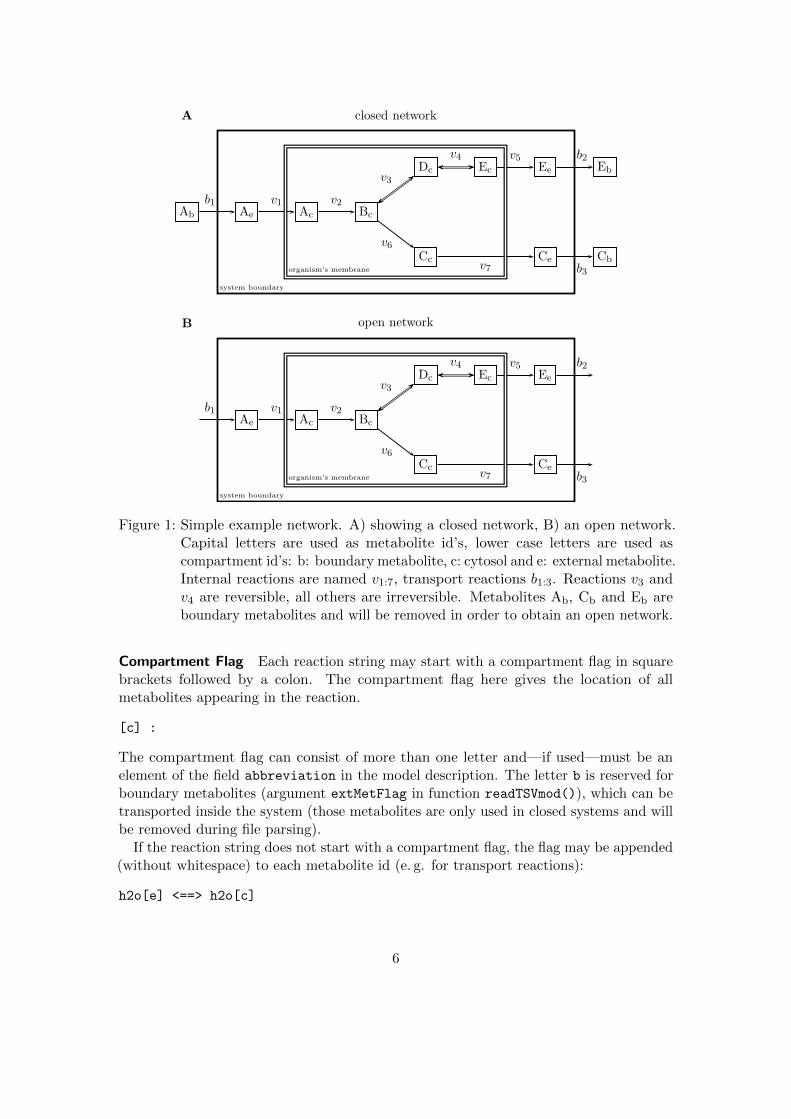
Figure 1: Simple example network. A) showing a closed network, B) an open network.Capital letters are used as metabolite id’s, lower case letters are used ascompartment id’s: b: boundary metabolite, c: cytosol and e: external metabolite.Internal reactions are named v1:7, transport reactions b1:3. Reactions v3 andv4 are reversible, all others are irreversible. Metabolites Ab, Cb and Eb areboundary metabolites and will be removed in order to obtain an open network.

Compartment Flag Each reaction string may start with a compartment flag in squarebrackets followed by a colon. The compartment flag here gives the location of allmetabolites appearing in the reaction.

[c] :

The compartment flag can consist of more than one letter and—if used—must be anelement of the field abbreviation in the model description. The letter b is reserved forboundary metabolites (argument extMetFlag in function readTSVmod()), which can betransported inside the system (those metabolites are only used in closed systems and willbe removed during file parsing).

If the reaction string does not start with a compartment flag, the flag may be appended(without whitespace) to each metabolite id (e. g. for transport reactions):

h2o[e] <==> h2o[c]

6

If no compartment flag is found, it is set to [unknown].

Reaction Arrow All reactions must be written in the direction educt to product, sothat all metabolites left of the reaction arrow are considered as educts, all metabolites onthe right of the reaction arrow are products.

The reaction arrow itself consists of one or more = or - symbols. The last symbol mustbe a >. If a reaction arrow starts with <, it is taken as reversible, if the field reversible

in the reaction list is empty. If the field reversible is set to TRUE or Reversible, thereactions will be treated as a reversible reaction, independent of the reaction arrow. Eachreaction must contain exactly one reaction arrow.

Stoichiometric Coefficients Stoichiometric coefficients must be in round brackets infront of the corresponding metabolite:

(2) h[c] + (0.5) o2[c] + q8h2[c] --> h2o[c] + (2) h[e] + q8[c]

Setting the stoichiometric coefficient in brackets makes it possible for the metabolite idto start with a number.

Metabolite Id’s The abbreviation of a metabolite name (a metabolite id) must beunique for the model and must not contain +, ( or ) characters.

Examples A minimal reaction list without compartment flags for figure 1B (opennetwork):

equation

A --> B

B <==> D

D <==> E

B --> C

--> A

C -->

E -->

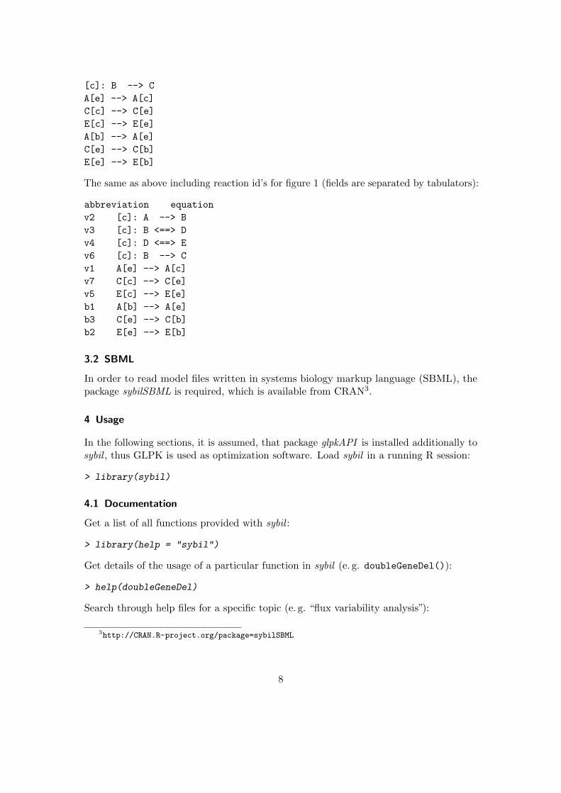
The same as above including compartment flags and external metabolites and all transportreactions for figure 1A (closed network). The reactions which take place in only onecompartment (do not include a transport of metabolites across membranes) have theircompartment flag at the beginning of the line ([c] in this example). For transportreactions all metabolites have their own compartment flag, e. g. in line 5 metabolite A istransported from compartment [e] (external) to compartment [c] (cytosol):

equation

[c]: A --> B

[c]: B <==> D

[c]: D <==> E

7

[c]: B --> C

A[e] --> A[c]

C[c] --> C[e]

E[c] --> E[e]

A[b] --> A[e]

C[e] --> C[b]

E[e] --> E[b]

The same as above including reaction id’s for figure 1 (fields are separated by tabulators):

abbreviation equation

v2 [c]: A --> B

v3 [c]: B <==> D

v4 [c]: D <==> E

v6 [c]: B --> C

v1 A[e] --> A[c]

v7 C[c] --> C[e]

v5 E[c] --> E[e]

b1 A[b] --> A[e]

b3 C[e] --> C[b]

b2 E[e] --> E[b]

3.2 SBML

In order to read model files written in systems biology markup language (SBML), thepackage sybilSBML is required, which is available from CRAN3.

4 Usage

In the following sections, it is assumed, that package glpkAPI is installed additionally tosybil , thus GLPK is used as optimization software. Load sybil in a running R session:

> library(sybil)

4.1 Documentation

Get a list of all functions provided with sybil :

> library(help = "sybil")

Get details of the usage of a particular function in sybil (e. g. doubleGeneDel()):

> help(doubleGeneDel)

Search through help files for a specific topic (e. g. “flux variability analysis”):

3http://CRAN.R-project.org/package=sybilSBML

8

http://CRAN.R-project.org/package=sybilSBML

> help.search("flux variability analysis")

Open this vignette:

> vignette("sybil")

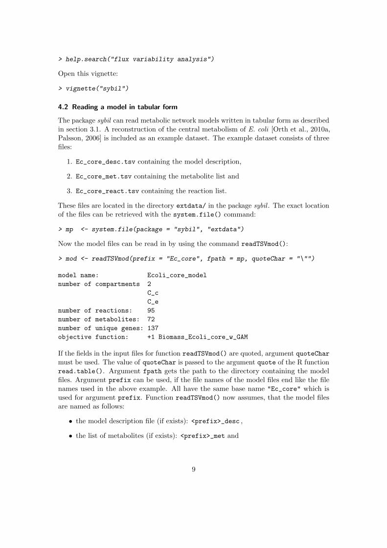
4.2 Reading a model in tabular form

The package sybil can read metabolic network models written in tabular form as describedin section 3.1. A reconstruction of the central metabolism of E. coli [Orth et al., 2010a,Palsson, 2006] is included as an example dataset. The example dataset consists of threefiles:

1. Ec_core_desc.tsv containing the model description,

2. Ec_core_met.tsv containing the metabolite list and

3. Ec_core_react.tsv containing the reaction list.

These files are located in the directory extdata/ in the package sybil . The exact locationof the files can be retrieved with the system.file() command:

> mp <- system.file(package = "sybil", "extdata")

Now the model files can be read in by using the command readTSVmod():

> mod <- readTSVmod(prefix = "Ec_core", fpath = mp, quoteChar = "\"")

model name: Ecoli_core_model

number of compartments 2

C_c

C_e

number of reactions: 95

number of metabolites: 72

number of unique genes: 137

objective function: +1 Biomass_Ecoli_core_w_GAM

If the fields in the input files for function readTSVmod() are quoted, argument quoteCharmust be used. The value of quoteChar is passed to the argument quote of the R functionread.table(). Argument fpath gets the path to the directory containing the modelfiles. Argument prefix can be used, if the file names of the model files end like the filenames used in the above example. All have the same base name "Ec_core" which isused for argument prefix. Function readTSVmod() now assumes, that the model filesare named as follows:

• the model description file (if exists): <prefix>_desc ,

• the list of metabolites (if exists): <prefix>_met and

9

• the list of reactions (must be there): <prefix>_react .

The file name suffix depends on the field delimiter. If the fields are tab-delimited, thedefault is .tsv . Function readTSVmod() returns an object of class modelorg. Models(instances of class modelorg, see section 5.1) can be converted to files in tabular formwith the command modelorg2tsv:

> modelorg2tsv(mod, prefix = "Ec_core")

This will generate the three files shown in the list above (see also section 3.1). Load theexample dataset included in sybil .

> data(Ec_core)

The example model is a ‘ready to use’ model, it contains a biomass objective functionand an uptake of glucose [Orth et al., 2010a, Palsson, 2006]. It is the same model as usedin the text files before.

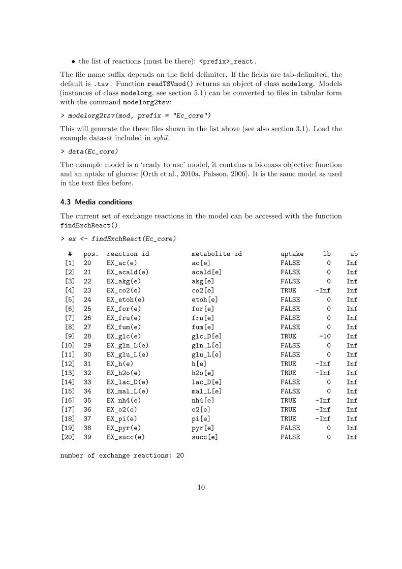
4.3 Media conditions

The current set of exchange reactions in the model can be accessed with the functionfindExchReact().

> ex <- findExchReact(Ec_core)

# pos. reaction id metabolite id uptake lb ub

[1] 20 EX_ac(e) ac[e] FALSE 0 Inf

[2] 21 EX_acald(e) acald[e] FALSE 0 Inf

[3] 22 EX_akg(e) akg[e] FALSE 0 Inf

[4] 23 EX_co2(e) co2[e] TRUE -Inf Inf

[5] 24 EX_etoh(e) etoh[e] FALSE 0 Inf

[6] 25 EX_for(e) for[e] FALSE 0 Inf

[7] 26 EX_fru(e) fru[e] FALSE 0 Inf

[8] 27 EX_fum(e) fum[e] FALSE 0 Inf

[9] 28 EX_glc(e) glc_D[e] TRUE -10 Inf

[10] 29 EX_gln_L(e) gln_L[e] FALSE 0 Inf

[11] 30 EX_glu_L(e) glu_L[e] FALSE 0 Inf

[12] 31 EX_h(e) h[e] TRUE -Inf Inf

[13] 32 EX_h2o(e) h2o[e] TRUE -Inf Inf

[14] 33 EX_lac_D(e) lac_D[e] FALSE 0 Inf

[15] 34 EX_mal_L(e) mal_L[e] FALSE 0 Inf

[16] 35 EX_nh4(e) nh4[e] TRUE -Inf Inf

[17] 36 EX_o2(e) o2[e] TRUE -Inf Inf

[18] 37 EX_pi(e) pi[e] TRUE -Inf Inf

[19] 38 EX_pyr(e) pyr[e] FALSE 0 Inf

[20] 39 EX_succ(e) succ[e] FALSE 0 Inf

number of exchange reactions: 20

10

The subset of uptake reactions can be retrieved by method uptReact.

> upt <- uptReact(ex)

[1] "EX_co2(e)" "EX_glc(e)" "EX_h(e)" "EX_h2o(e)" "EX_nh4(e)" "EX_o2(e)"

[7] "EX_pi(e)"

> ex[upt]



[2] 28 EX_glc(e) glc_D[e] TRUE -10 Inf







Function findExchReact() returns an object of class reactId_Exch (extending classreactId) which can be used to alter reaction bounds with function changeBounds().Make lactate the main carbon source instead of glucose:

> mod <- changeBounds(Ec_core, ex[c("EX_glc(e)", "EX_lac_D(e)")], lb = c(0, -10))

> findExchReact(mod)








[7] 26 EX_fru(e) fru[e] FALSE 0 Inf

[8] 27 EX_fum(e) fum[e] FALSE 0 Inf

[9] 28 EX_glc(e) glc_D[e] FALSE 0 Inf





[14] 33 EX_lac_D(e) lac_D[e] TRUE -10 Inf




11





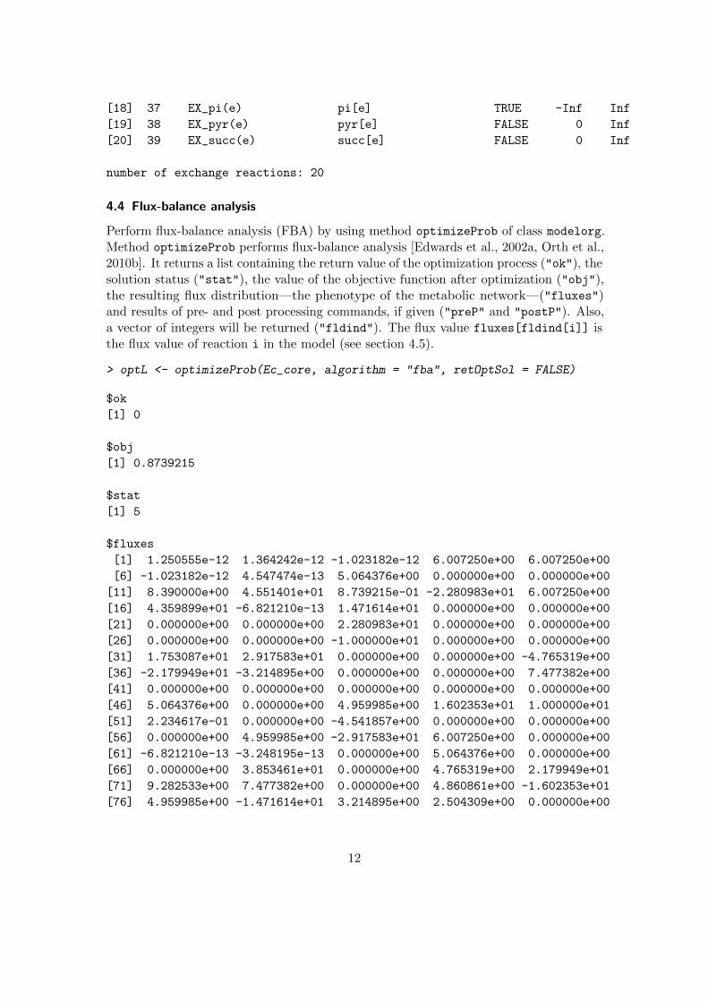
4.4 Flux-balance analysis

Perform flux-balance analysis (FBA) by using method optimizeProb of class modelorg.Method optimizeProb performs flux-balance analysis [Edwards et al., 2002a, Orth et al.,2010b]. It returns a list containing the return value of the optimization process ("ok"), thesolution status ("stat"), the value of the objective function after optimization ("obj"),the resulting flux distribution—the phenotype of the metabolic network—("fluxes")and results of pre- and post processing commands, if given ("preP" and "postP"). Also,a vector of integers will be returned ("fldind"). The flux value fluxes[fldind[i]] isthe flux value of reaction i in the model (see section 4.5).

> optL <- optimizeProb(Ec_core, algorithm = "fba", retOptSol = FALSE)

$ok

[1] 0

$obj

[1] 0.8739215

$stat

[1] 5

$fluxes

[1] 1.250555e-12 1.364242e-12 -1.023182e-12 6.007250e+00 6.007250e+00

[6] -1.023182e-12 4.547474e-13 5.064376e+00 0.000000e+00 0.000000e+00

[11] 8.390000e+00 4.551401e+01 8.739215e-01 -2.280983e+01 6.007250e+00

[16] 4.359899e+01 -6.821210e-13 1.471614e+01 0.000000e+00 0.000000e+00

[21] 0.000000e+00 0.000000e+00 2.280983e+01 0.000000e+00 0.000000e+00

[26] 0.000000e+00 0.000000e+00 -1.000000e+01 0.000000e+00 0.000000e+00

[31] 1.753087e+01 2.917583e+01 0.000000e+00 0.000000e+00 -4.765319e+00

[36] -2.179949e+01 -3.214895e+00 0.000000e+00 0.000000e+00 7.477382e+00

[41] 0.000000e+00 0.000000e+00 0.000000e+00 0.000000e+00 0.000000e+00

[46] 5.064376e+00 0.000000e+00 4.959985e+00 1.602353e+01 1.000000e+01

[51] 2.234617e-01 0.000000e+00 -4.541857e+00 0.000000e+00 0.000000e+00

[56] 0.000000e+00 4.959985e+00 -2.917583e+01 6.007250e+00 0.000000e+00

[61] -6.821210e-13 -3.248195e-13 0.000000e+00 5.064376e+00 0.000000e+00

[66] 0.000000e+00 3.853461e+01 0.000000e+00 4.765319e+00 2.179949e+01

[71] 9.282533e+00 7.477382e+00 0.000000e+00 4.860861e+00 -1.602353e+01

[76] 4.959985e+00 -1.471614e+01 3.214895e+00 2.504309e+00 0.000000e+00

12

[81] 0.000000e+00 -2.046363e-12 1.758177e+00 0.000000e+00 2.678482e+00

[86] -2.281503e+00 8.881784e-16 0.000000e+00 5.064376e+00 -5.064376e+00

[91] 1.496984e+00 0.000000e+00 1.496984e+00 1.181498e+00 7.477382e+00

$preP

[1] NA

$postP

[1] NA

$fldind

[1] 1 2 3 4 5 6 7 8 9 10 11 12 13 14 15 16 17 18 19 20 21 22 23 24 25

[26] 26 27 28 29 30 31 32 33 34 35 36 37 38 39 40 41 42 43 44 45 46 47 48 49 50

[51] 51 52 53 54 55 56 57 58 59 60 61 62 63 64 65 66 67 68 69 70 71 72 73 74 75

[76] 76 77 78 79 80 81 82 83 84 85 86 87 88 89 90 91 92 93 94 95

Perform FBA, return an object of class optsol_optimizeProb (extends class optsol,see section 5.2, this is the default behavior).

> opt <- optimizeProb(Ec_core, algorithm = "fba", retOptSol = TRUE)

solver: glpkAPI

method: simplex

algorithm: fba

number of variables: 95

number of constraints: 72

return value of solver: solution process was successful

solution status: solution is optimal

value of objective function (fba): 0.873922

value of objective function (model): 0.873922

The variable opt contains an object of class optsol_optimizeProb, a data structurestoring all results of the optimization and providing methods to access the data (seesection 5.2). Retrieve the value of the objective function after optimization.

> lp_obj(opt)

[1] 0.8739215

Translate the return and status codes of the optimization software into human readablestrings.

> checkOptSol(opt)

Return code:

Code # meaning

13

0 1 solution process was successful

Solution status:

Code # meaning

5 1 solution is optimal

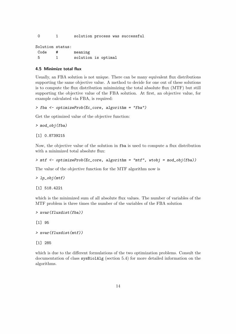
4.5 Minimize total flux

Usually, an FBA solution is not unique. There can be many equivalent flux distributionssupporting the same objective value. A method to decide for one out of these solutionsis to compute the flux distribution minimizing the total absolute flux (MTF) but stillsupporting the objective value of the FBA solution. At first, an objective value, forexample calculated via FBA, is required:

> fba <- optimizeProb(Ec_core, algorithm = "fba")

Get the optimized value of the objective function:

> mod_obj(fba)

[1] 0.8739215

Now, the objective value of the solution in fba is used to compute a flux distributionwith a minimized total absolute flux:

> mtf <- optimizeProb(Ec_core, algorithm = "mtf", wtobj = mod_obj(fba))

The value of the objective function for the MTF algorithm now is

> lp_obj(mtf)

[1] 518.4221

which is the minimized sum of all absolute flux values. The number of variables of theMTF problem is three times the number of the variables of the FBA solution

> nvar(fluxdist(fba))

[1] 95

> nvar(fluxdist(mtf))

[1] 285

which is due to the different formulations of the two optimization problems. Consult thedocumentation of class sysBiolAlg (section 5.4) for more detailed information on thealgorithms.

14

> help("sysBiolAlg_fba-class")

> help("sysBiolAlg_mtf-class")

There are also shortcuts available:

> ?fba

> ?mtf

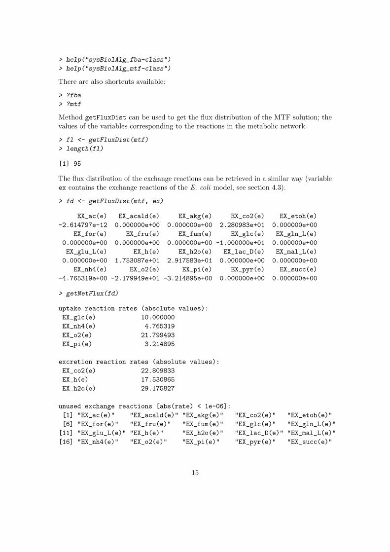
Method getFluxDist can be used to get the flux distribution of the MTF solution; thevalues of the variables corresponding to the reactions in the metabolic network.

> fl <- getFluxDist(mtf)

> length(fl)

[1] 95

The flux distribution of the exchange reactions can be retrieved in a similar way (variableex contains the exchange reactions of the E. coli model, see section 4.3).

> fd <- getFluxDist(mtf, ex)

EX_ac(e) EX_acald(e) EX_akg(e) EX_co2(e) EX_etoh(e)

-2.614797e-12 0.000000e+00 0.000000e+00 2.280983e+01 0.000000e+00

EX_for(e) EX_fru(e) EX_fum(e) EX_glc(e) EX_gln_L(e)

0.000000e+00 0.000000e+00 0.000000e+00 -1.000000e+01 0.000000e+00

EX_glu_L(e) EX_h(e) EX_h2o(e) EX_lac_D(e) EX_mal_L(e)

0.000000e+00 1.753087e+01 2.917583e+01 0.000000e+00 0.000000e+00

EX_nh4(e) EX_o2(e) EX_pi(e) EX_pyr(e) EX_succ(e)

-4.765319e+00 -2.179949e+01 -3.214895e+00 0.000000e+00 0.000000e+00

> getNetFlux(fd)

uptake reaction rates (absolute values):

EX_glc(e) 10.000000

EX_nh4(e) 4.765319

EX_o2(e) 21.799493

EX_pi(e) 3.214895

excretion reaction rates (absolute values):

EX_co2(e) 22.809833

EX_h(e) 17.530865

EX_h2o(e) 29.175827

unused exchange reactions [abs(rate) < 1e-06]:

[1] "EX_ac(e)" "EX_acald(e)" "EX_akg(e)" "EX_co2(e)" "EX_etoh(e)"

[6] "EX_for(e)" "EX_fru(e)" "EX_fum(e)" "EX_glc(e)" "EX_gln_L(e)"

[11] "EX_glu_L(e)" "EX_h(e)" "EX_h2o(e)" "EX_lac_D(e)" "EX_mal_L(e)"

[16] "EX_nh4(e)" "EX_o2(e)" "EX_pi(e)" "EX_pyr(e)" "EX_succ(e)"

15

Function getNetFlux() the absolute flux values of the exchange reactions grouped byflux direction. The value of the objective function given in the model (here: biomassproduction) can be accessed by method mod_obj:

> mod_obj(mtf)

[1] 0.8739215

which is of course the same value as for the FBA algorithm.

4.6 Example: Limit intake by carbon atom number (easyConstraint)

This example is meant to demonstrate the usage of the classes sysBiolAlg_fbaEasyConstraintand sysBiolAlg_mtfEasyConstraint. These two algorithms work like the normal FBAand MTF, but also have the ability to easily add additional linear constraints to thelinear programm. So the ith constraint woult look like follows:

γi ≤ vri ∗ xTi ≤ δi

With γ and δ beeing the vectors of upper and lower bounds, v is flux vector and r andx are sets of vectors indicating the affected reactions and the corresponding coefficients,respectively.

In our example we want to limit the carbon intake on basis of the C-atoms in themolekules: we only allow uptake for glucose (6 carbon atoms), fumarate (4 carbon atoms),and fructose (4 carbons). Thus we can find the preffered carbon source of the model.

> data(Ec_core)

> optimizeProb(Ec_core)

solver: glpkAPI

method: simplex

algorithm: fba







> Ec_core_C <- Ec_core # we copy the model to compare later.

> # define carbon sources...

> CS_List = c('EX_fru(e)' , 'EX_glc(e)', 'EX_fum(e)')> CS_CA = c(6,6,4); # ...and the number of carbon atoms per molekule

> cntCAtoms = 6 * abs(lowbnd(Ec_core_C)[react_id(Ec_core_C)=='EX_glc(e)'])> # prohibit excretion of carbon sources

> uppbnd(Ec_core_C)[react_id(Ec_core_C) %in% CS_List] = 0

16

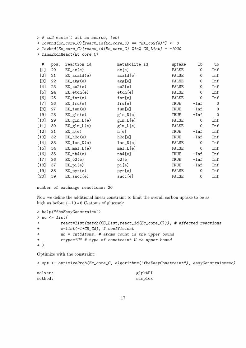
> # co2 mustn't act as source, too!

> lowbnd(Ec_core_C)[react_id(Ec_core_C) == "EX_co2(e)"] <- 0

> lowbnd(Ec_core_C)[react_id(Ec_core_C) %in% CS_List] = -1000

> findExchReact(Ec_core_C)





[4] 23 EX_co2(e) co2[e] FALSE 0 Inf



[7] 26 EX_fru(e) fru[e] TRUE -Inf 0

[8] 27 EX_fum(e) fum[e] TRUE -Inf 0

[9] 28 EX_glc(e) glc_D[e] TRUE -Inf 0





[14] 33 EX_lac_D(e) lac_D[e] FALSE 0 Inf








Now we define the additional linear constraint to limit the overall carbon uptake to be ashigh as before (−10 ∗ 6 C-atoms of glucose):

> help("fbaEasyConstraint")

> ec <- list(

+ react=list(match(CS_List,react_id(Ec_core_C))), # affected reactions

+ x=list(-1*CS_CA), # coefficient

+ ub = cntCAtoms, # atoms count is the upper bound

+ rtype="U" # type of constraint U => upper bound

+ )

Optimize with the constraint:

> opt <- optimizeProb(Ec_core_C, algorithm=("fbaEasyConstraint"), easyConstraint=ec)

solver: glpkAPI

method: simplex

17

algorithm: fba







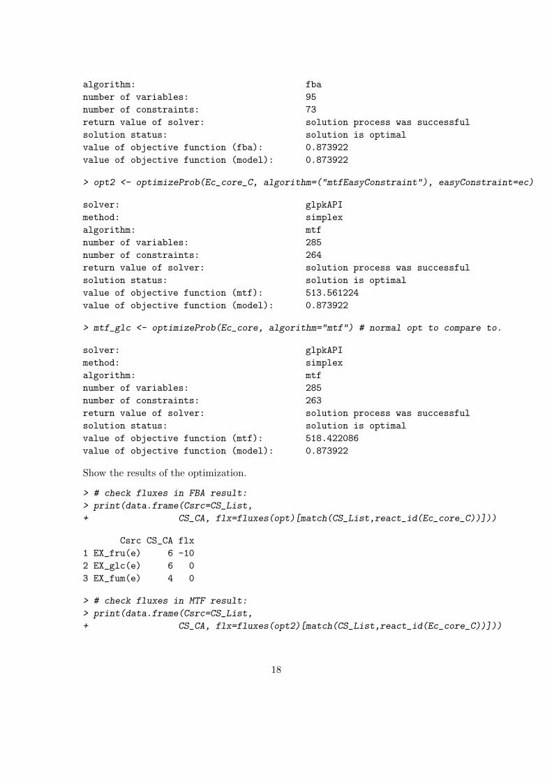
> opt2 <- optimizeProb(Ec_core_C, algorithm=("mtfEasyConstraint"), easyConstraint=ec)

solver: glpkAPI

method: simplex

algorithm: mtf





value of objective function (mtf): 513.561224


> mtf_glc <- optimizeProb(Ec_core, algorithm="mtf") # normal opt to compare to.

solver: glpkAPI

method: simplex

algorithm: mtf





value of objective function (mtf): 518.422086


Show the results of the optimization.

> # check fluxes in FBA result:

> print(data.frame(Csrc=CS_List,

+ CS_CA, flx=fluxes(opt)[match(CS_List,react_id(Ec_core_C))]))

Csrc CS_CA flx

1 EX_fru(e) 6 -10

2 EX_glc(e) 6 0

3 EX_fum(e) 4 0

> # check fluxes in MTF result:

> print(data.frame(Csrc=CS_List,

+ CS_CA, flx=fluxes(opt2)[match(CS_List,react_id(Ec_core_C))]))

18

Csrc CS_CA flx

1 EX_fru(e) 6 -4.860861e+00

2 EX_glc(e) 6 -5.139139e+00

3 EX_fum(e) 4 1.841727e-11

> # look at biomass values:

> print(data.frame(fbaCA=mod_obj(opt),

+ mtfCA=mod_obj(opt2), mtf_glc=mod_obj(mtf_glc)))

fbaCA mtfCA mtf_glc

1 0.8739215 0.8739215 0.8739215

> # compare the absolute sum over fluxes

> print(data.frame(mtfCA=lp_obj(opt2), mtf_glc=lp_obj(mtf_glc)))

mtfCA mtf_glc

1 513.5612 518.4221

> # write problem to file (optional)

> prob <- sysBiolAlg(Ec_core_C, algorithm = "fbaEasyConstraint",

+ easyConstraint=ec, useNames=TRUE)

> writeProb(problem(prob), fname='test_easyCons.lp')

[1] TRUE

4.7 Genetic perturbations

To compute the metabolic phenotypes of in silico knock-out mutants, argument gene ofmethod optimizeProb can be used.

> ko <- optimizeProb(Ec_core, gene = "b2276", lb = 0, ub = 0)

solver: glpkAPI

method: simplex

algorithm: fba







Argument gene gets a character vector of gene locus tags present in the used model. Theflux boundaries of reactions affected by the genes given in argument gene will be set tothe values of arguments lb and ub. If both arguments are set to zero, no flux throughthe affected reactions is allowed.

19

4.7.1 Minimization of metabolic adjustment (MOMA)

The default algorithm used by method optimizeProb is FBA [Edwards et al., 2002a,Orth et al., 2010b], implying the assumption, that the phenotype of the mutant metabolicnetwork is independent of the wild-type phenotype. An alternative is the MOMAalgorithm described in Segre et al. [2002] minimizing the hamiltonian distance of the wild-type phenotype and the mutant phenotype (argument algorithm = "lmoma" computesa linearized version of the MOMA algorithm; algorithm = "moma" runs the quadraticformulation).

> ko <- optimizeProb(Ec_core, gene = "b2276", lb = 0, ub = 0,

+ algorithm = "lmoma", wtflux = getFluxDist(mtf))

solver: glpkAPI

method: simplex

algorithm: lmoma





value of objective function (lmoma): 424.324062


The variable ko contains the solution of the linearized version of the MOMA algorithm.A wild-type flux distribution can be set via argument wtflux, here, the flux distributioncomputed through the MTF algorithm was used. If argument wtflux is not set, a fluxdistribution based on FBA will be used.

4.7.2 Regulatory on/off minimization (ROOM)

Another alternative is the ROOM algorithm (regulatory on/off minimization) describedin Shlomi et al. [2005]. Set argument algorithm to room in order to run ROOM.

> ko <- optimizeProb(Ec_core, gene = "b2276", lb = 0, ub = 0,

+ algorithm = "room", wtflux = getFluxDist(mtf),

+ solverParm = list(PRESOLVE = GLP_ON))

ROOM is a mixed integer programming problem which requires for GLPK to switchon the pre-solver. See section 4.15 for more information on setting parameters to themathematical programming software.

4.7.3 Multiple knock-outs

Method optimizeProb can be used to study the metabolic phenotype of one knock-out mu-tant. The purpose of functions oneGeneDel(), doubleGeneDel() and geneDeletion()

is the simulation of multiple in silico knock-outs (see table 2). Function oneGeneDel()

simulates all possible single gene knock-out mutants in a metabolic model (defaultalgorithm is FBA).

20

Table 2: Functions used to simulate multiple in silico knock-out mutants.

function purpose

oneGeneDel() single gene knock-outsdoubleGeneDel() pairwise gene knock-outsgeneDeletion() simultaneous deletion of n genes

> opt <- oneGeneDel(Ec_core)

| : | : | 100 %

|===================================================| :-)

solver: glpkAPI

method: simplex

algorithm: fba



number of problems to solve: 137

number of successful solution processes: 137

The function oneGeneDel gets an argument geneList, a character vector containing thegene id’s to knock out. If geneList is missing, all genes are taken into account. Theexample model contains 137 independent genes, so 137 optimizations will be performed.

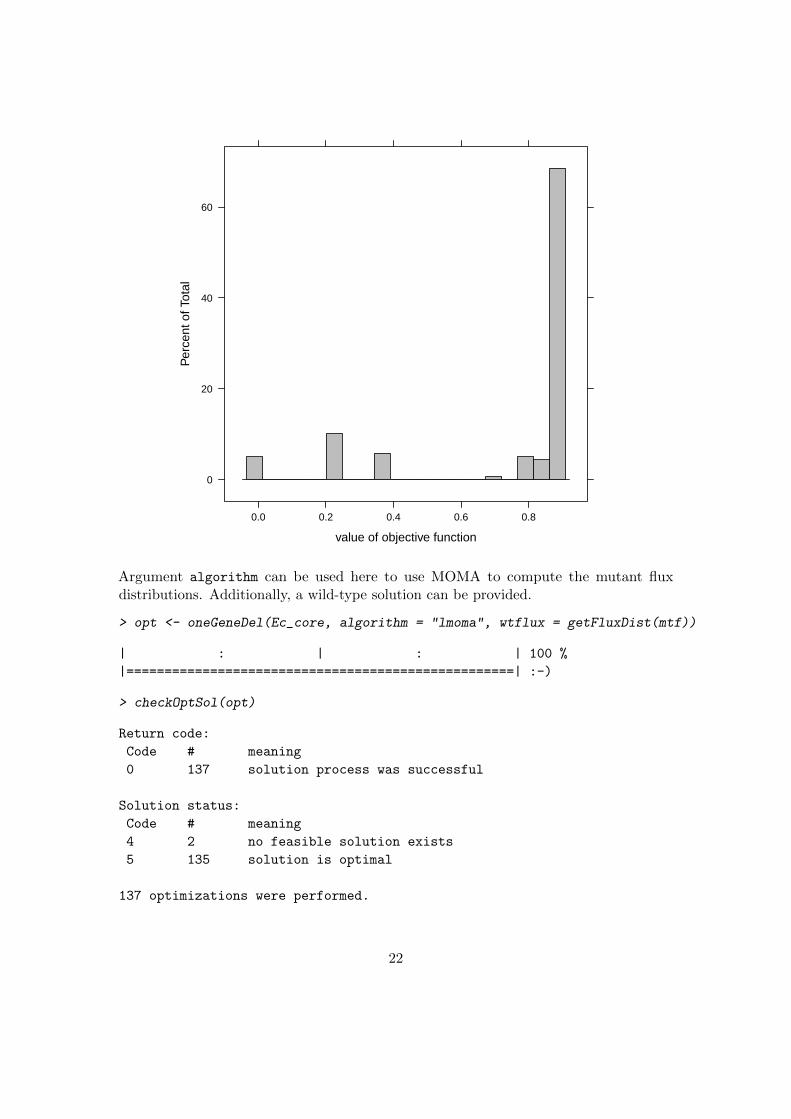
The result stored in the variable opt is an object of class optsol_geneDel, extendingclass optsol_optimizeProb (see section 4.4). Method checkOptSol gives an overviewabout the results and status of the optimizations. Additionally, class optsol contains amethod plot, plotting a histogram of the values of the objective function given in themodel after optimization (section 5.2).

> checkOptSol(opt)

Return code:

Code # meaning


Solution status:

Code # meaning

4 2 no feasible solution exists


137 optimizations were performed.

Plot the histogram:

> plot(opt, nint = 20)

21

value of objective function

Per

cent

of T

otal

0

20

40

60

0.0 0.2 0.4 0.6 0.8

Argument algorithm can be used here to use MOMA to compute the mutant fluxdistributions. Additionally, a wild-type solution can be provided.

> opt <- oneGeneDel(Ec_core, algorithm = "lmoma", wtflux = getFluxDist(mtf))

| : | : | 100 %

|===================================================| :-)

> checkOptSol(opt)

Return code:

Code # meaning


Solution status:

Code # meaning




22

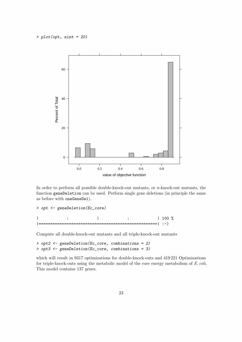
> plot(opt, nint = 20)

value of objective function

Per

cent

of T

otal

0

20

40

60

0.0 0.2 0.4 0.6 0.8

In order to perform all possible double-knock-out mutants, or n-knock-out mutants, thefunction geneDeletion can be used. Perform single gene deletions (in principle the sameas before with oneGeneDel).

> opt <- geneDeletion(Ec_core)

| : | : | 100 %

|===================================================| :-)

Compute all double-knock-out mutants and all triple-knock-out mutants

> opt2 <- geneDeletion(Ec_core, combinations = 2)

> opt3 <- geneDeletion(Ec_core, combinations = 3)

which will result in 9317 optimizations for double-knock-outs and 419 221 Optimizationsfor triple-knock-outs using the metabolic model of the core energy metabolism of E. coli.This model contains 137 genes.

23

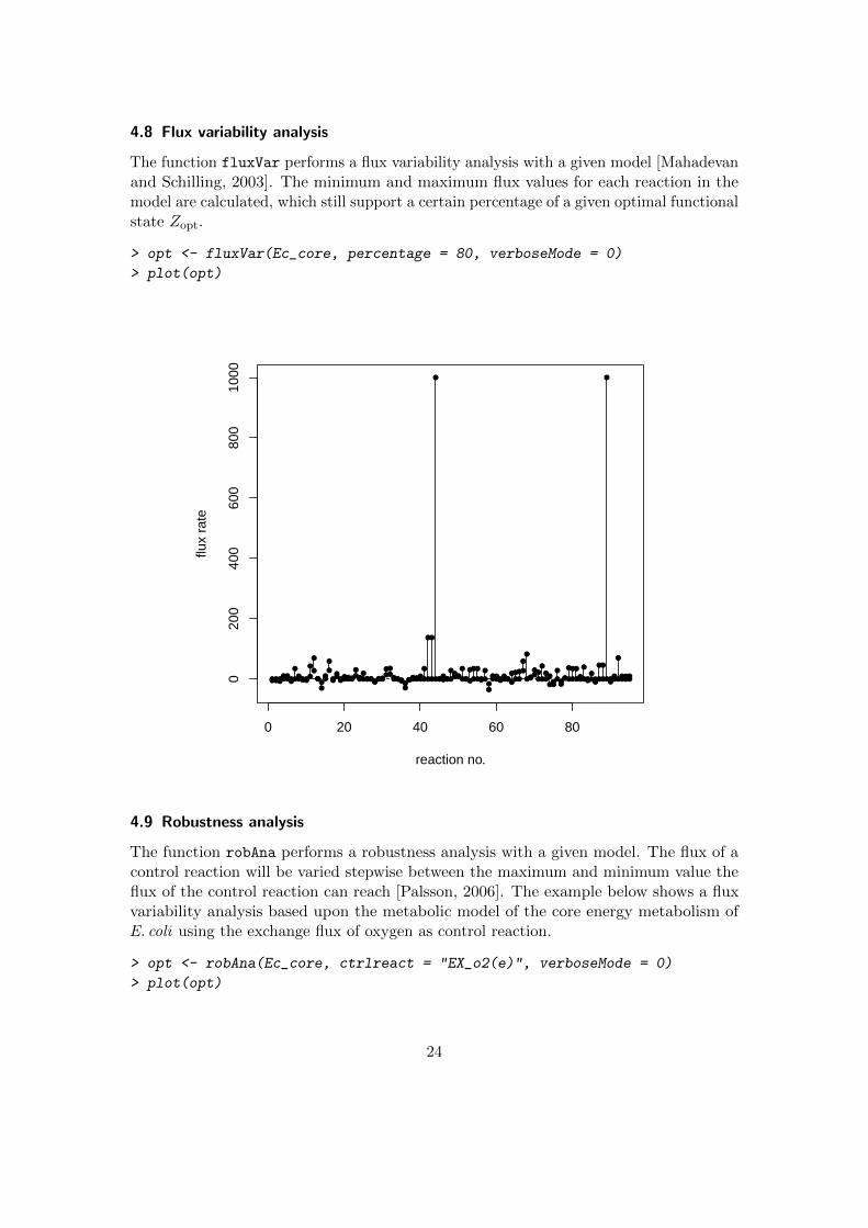
4.8 Flux variability analysis

The function fluxVar performs a flux variability analysis with a given model [Mahadevanand Schilling, 2003]. The minimum and maximum flux values for each reaction in themodel are calculated, which still support a certain percentage of a given optimal functionalstate Zopt.

> opt <- fluxVar(Ec_core, percentage = 80, verboseMode = 0)

> plot(opt)

●●●●●●●●●●●

●

●

●

●

●

●●

●●●●●

●●●●●

●●●●

●●●

●

●●●●●●●●●●●●●●●●●●●●●

●

●●●●●●

●●

●

●●●

●●●●●

●●

●●●●●●●●●

●●●●

●●●●●●●●●●

●

●

●●●

●

●

●●

●

●

●●

●●●●

●

●●

●●●●●

●●

●●●●

●●●●

●

●●

●

●●

●

●●●

●

●

●●●

●

●

●

●●●

●●

●●●

●

●

●

●●●

●●

●

●

●●

●●●

●

●

●●

●

●●

●

●●

●

●●●

0 20 40 60 80

020

040

060

080

010

00

reaction no.

flux

rate

4.9 Robustness analysis

The function robAna performs a robustness analysis with a given model. The flux of acontrol reaction will be varied stepwise between the maximum and minimum value theflux of the control reaction can reach [Palsson, 2006]. The example below shows a fluxvariability analysis based upon the metabolic model of the core energy metabolism ofE. coli using the exchange flux of oxygen as control reaction.

> opt <- robAna(Ec_core, ctrlreact = "EX_o2(e)", verboseMode = 0)

> plot(opt)

24

0 10 20 30 40 50 60

0.0

0.2

0.4

0.6

0.8

Control Flux: EX_o2(e)

Obj

ectiv

e F

unct

ion:

+1

Bio

mas

s_E

coli_

core

_w_G

AM

●

●

●

●

●

●

●

●

●

●

●

●

●

●

●

●

●

●

●

●

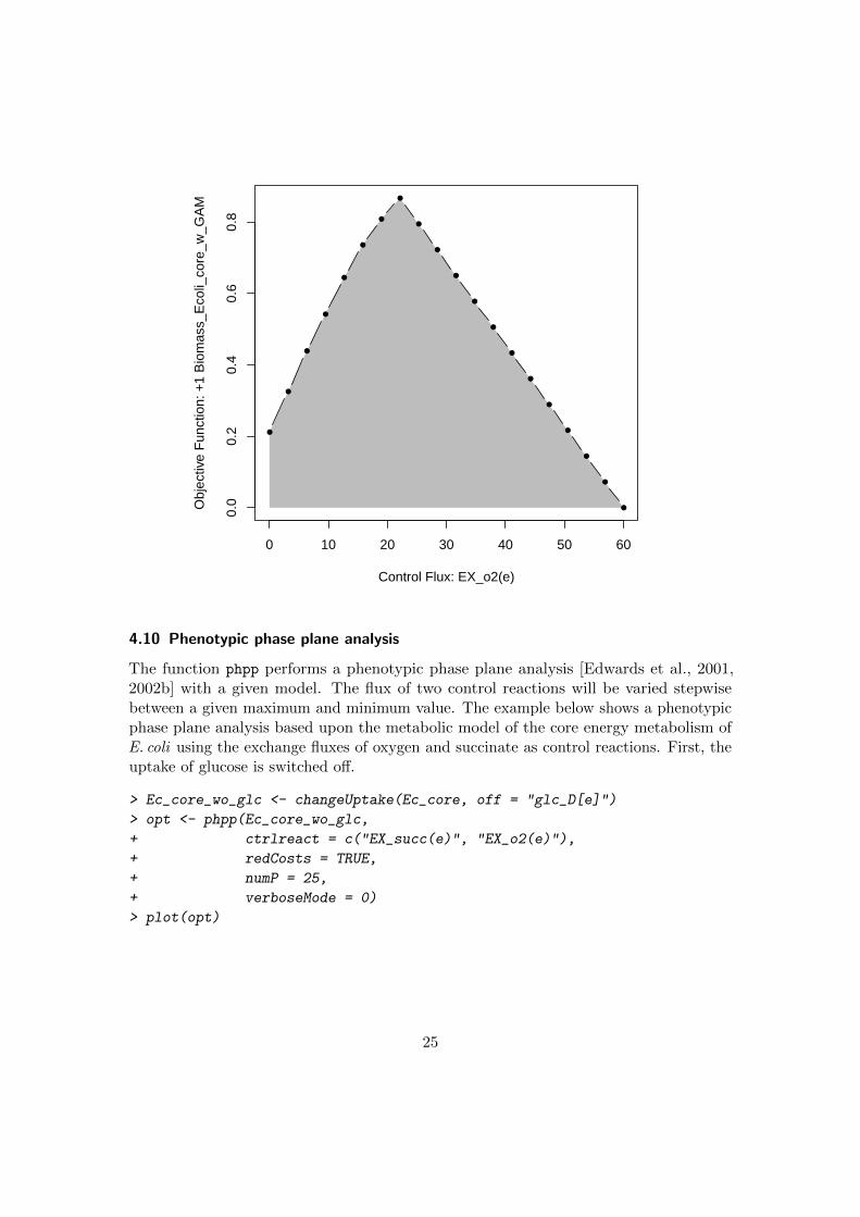
4.10 Phenotypic phase plane analysis

The function phpp performs a phenotypic phase plane analysis [Edwards et al., 2001,2002b] with a given model. The flux of two control reactions will be varied stepwisebetween a given maximum and minimum value. The example below shows a phenotypicphase plane analysis based upon the metabolic model of the core energy metabolism ofE. coli using the exchange fluxes of oxygen and succinate as control reactions. First, theuptake of glucose is switched off.

> Ec_core_wo_glc <- changeUptake(Ec_core, off = "glc_D[e]")

> opt <- phpp(Ec_core_wo_glc,

+ ctrlreact = c("EX_succ(e)", "EX_o2(e)"),

+ redCosts = TRUE,

+ numP = 25,

+ verboseMode = 0)

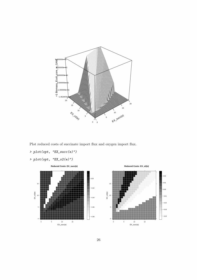
> plot(opt)

25

0

5

10

15

20

0

5

10

15

20

−1.953497e−14

1.000000e−01

2.000000e−01

3.000000e−01

4.000000e−01

5.000000e−01

EX_succ(e)EX_o2(e)

+1

Bio

mas

s_E

coli_

core

_w_G

AM

Plot reduced costs of succinate import flux and oxygen import flux.

> plot(opt, "EX_succ(e)")

> plot(opt, "EX_o2(e)")

Reduced Costs: EX_succ(e)

EX_succ(e)

EX

_o2(

e)

0

5

10

15

0 5 10 15

−0.08

−0.06

−0.04

−0.02

0.00

Reduced Costs: EX_o2(e)

EX_succ(e)

EX

_o2(

e)

0

5

10

15

0 5 10 15

−0.04

−0.03

−0.02

−0.01

0.00

0.01

0.02

26

4.11 Summarizing simulation results

Each simulation generates an object of class optsol containing all the results of the opti-mizations. In order to get a quick overview of the results, the function summaryOptsol()

can be used. At first, let’s compute all single gene knock-outs of the metabolic model ofthe core energy metabolism of E. coli :

> opt <- oneGeneDel(Ec_core, algorithm = "fba", fld = "all")

| : | : | 100 %

|===================================================| :-)

Generate a summary:

> sum <- summaryOptsol(opt, Ec_core)

flux distribution:

number of elements: 13015

number of zeros: 6140

number of non zero elements: 6875

exchange metabolites:

[1] ac[e] acald[e] akg[e] co2[e] etoh[e] for[e] fru[e] fum[e]

[9] glc_D[e] gln_L[e] glu_L[e] h[e] h2o[e] lac_D[e] mal_L[e] nh4[e]

[17] o2[e] pi[e] pyr[e] succ[e]

substrates (-) and products (+):

use method ‘printExchange()’

limiting reactions:

there is about one limiting reaction per optimization;

use method ‘printReaction()’ to see more details

optimal values of model objective function:

Min. 1st Qu. Median Mean 3rd Qu. Max.

0.0000 0.8143 0.8739 0.7263 0.8739 0.8739

summary of optimization process:

Return code:

Code # meaning


Solution status:

Code # meaning



27


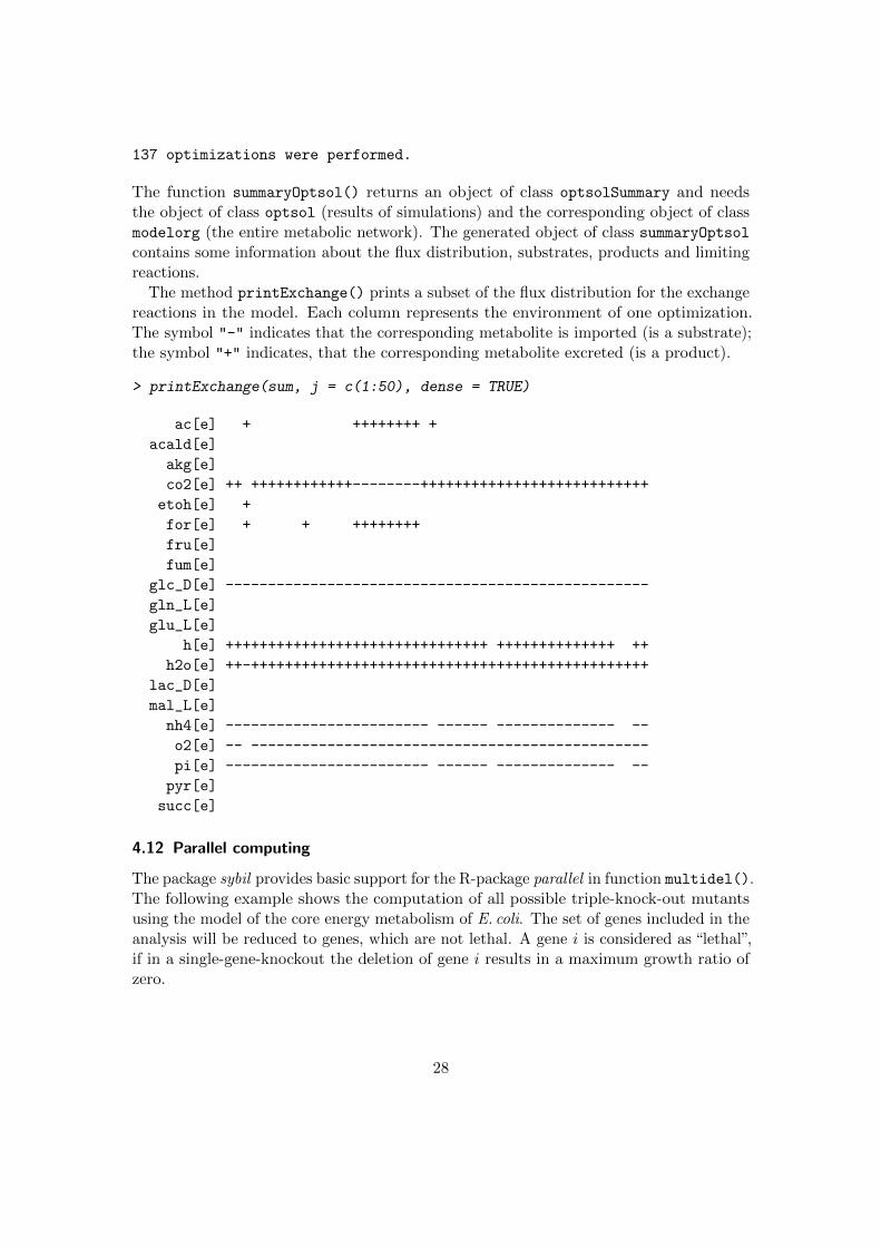
The function summaryOptsol() returns an object of class optsolSummary and needsthe object of class optsol (results of simulations) and the corresponding object of classmodelorg (the entire metabolic network). The generated object of class summaryOptsolcontains some information about the flux distribution, substrates, products and limitingreactions.

The method printExchange() prints a subset of the flux distribution for the exchangereactions in the model. Each column represents the environment of one optimization.The symbol "-" indicates that the corresponding metabolite is imported (is a substrate);the symbol "+" indicates, that the corresponding metabolite excreted (is a product).

> printExchange(sum, j = c(1:50), dense = TRUE)

ac[e] + ++++++++ +

acald[e]

akg[e]

co2[e] ++ ++++++++++++--------+++++++++++++++++++++++++++

etoh[e] +

for[e] + + ++++++++

fru[e]

fum[e]

glc_D[e] --------------------------------------------------

gln_L[e]

glu_L[e]

h[e] +++++++++++++++++++++++++++++++ ++++++++++++++ ++

h2o[e] ++-+++++++++++++++++++++++++++++++++++++++++++++++

lac_D[e]

mal_L[e]

nh4[e] ------------------------ ------ -------------- --

o2[e] -- -----------------------------------------------

pi[e] ------------------------ ------ -------------- --

pyr[e]

succ[e]

4.12 Parallel computing

The package sybil provides basic support for the R-package parallel in function multidel().The following example shows the computation of all possible triple-knock-out mutantsusing the model of the core energy metabolism of E. coli. The set of genes included in theanalysis will be reduced to genes, which are not lethal. A gene i is considered as “lethal”,if in a single-gene-knockout the deletion of gene i results in a maximum growth ratio ofzero.

28

> ref <- optimizeProb(Ec_core)

> opt <- oneGeneDel(Ec_core)

| : | : | 100 %

|===================================================| :-)

> let <- lethal(opt, wt = mod_obj(ref))

> nletid <- c(1:length(allGenes(Ec_core)))[! let]

At first, a wild-type maximum growth rate is computed and stored in the variable ref.Then, all single-gene knock-outs are computed. The variable let contains pointers tothe gene id’s of genes, who’s deletion is lethal. The variable nletid contains pointers tothe gene id’s of all genes, except for the lethal ones.

> gmat <- combn(nletid, 3)

The variable gmat now contains a matrix with three rows, each column is one combinationof three values in nletid; one set of genes to knock-out in one step.

> opt <- multiDel(Ec_core, nProc = 4, todo = "geneDeletion", del1 = gmat)

The function multiDel performs a geneDeletion with the model Ec_core on four CPU’s(argument nProc) on a shared memory machine. Argument del1 is the matrix containingthe sets of genes to delete. This matrix will be split up in smaller sub-matrices all havingabout the same number of columns and three rows. The sub-matrices are passed togeneDeletion and are processed on separate cores in parallel. The resulting variableopt now contains a list of four objects of class optsol_genedel. Use mapply to accessthe values stored in the optsol objects.

> mapply(checkOptSol, opt)

4.13 Interacting with the optimization process

Method optimizeProb provides a basic mechanism to run commands before and orafter solving the optimization problem. In order to retrieve the reduced costs after theoptimization, use argument poCmd.

> opt <- optimizeProb(Ec_core, poCmd = list("getRedCosts"))

> postProc(opt)

An object of class "ppProc"

Slot "cmd":

[[1]]

[1] "getRedCosts(LP_PROB)"

Slot "pa":

29

[[1]]

[1] 0.000000e+00 0.000000e+00 0.000000e+00 0.000000e+00 0.000000e+00

[6] 0.000000e+00 0.000000e+00 0.000000e+00 0.000000e+00 0.000000e+00

[11] -5.092486e-03 0.000000e+00 0.000000e+00 0.000000e+00 0.000000e+00

[16] 0.000000e+00 0.000000e+00 0.000000e+00 0.000000e+00 -2.291619e-02

[21] -3.437428e-02 -6.110983e-02 0.000000e+00 -3.946677e-02 0.000000e+00

[26] -9.166475e-02 -4.583237e-02 -9.166475e-02 -7.002168e-02 -6.874856e-02

[31] 0.000000e+00 0.000000e+00 -4.073989e-02 -4.583237e-02 0.000000e+00

[36] 0.000000e+00 0.000000e+00 -3.437428e-02 -4.837862e-02 0.000000e+00

[41] -5.092486e-03 0.000000e+00 -1.273121e-03 -4.718448e-16 0.000000e+00

[46] 0.000000e+00 0.000000e+00 0.000000e+00 0.000000e+00 0.000000e+00

[51] 0.000000e+00 0.000000e+00 0.000000e+00 -5.092486e-03 -5.092486e-03

[56] 0.000000e+00 0.000000e+00 0.000000e+00 0.000000e+00 -1.273121e-03

[61] 0.000000e+00 0.000000e+00 0.000000e+00 0.000000e+00 -5.092486e-03

[66] -3.819364e-03 0.000000e+00 -1.273121e-03 0.000000e+00 0.000000e+00

[71] 0.000000e+00 0.000000e+00 -6.365607e-03 0.000000e+00 0.000000e+00

[76] 0.000000e+00 0.000000e+00 0.000000e+00 0.000000e+00 -5.092486e-03

[81] -5.092486e-03 0.000000e+00 0.000000e+00 0.000000e+00 0.000000e+00

[86] 0.000000e+00 0.000000e+00 -3.819364e-03 0.000000e+00 0.000000e+00

[91] 0.000000e+00 -1.273121e-03 0.000000e+00 0.000000e+00 0.000000e+00

Slot "ind":

integer(0)

4.14 Optimization software

To solve optimization problems, GLPK4, IBM ILOG CPLEX5, COIN-OR Clp6 or lp solve7

can be used (package sybilGUROBI providing support for Gurobi optimization8 isavailable on request). All functions performing optimizations, get the arguments solverand method. The first setting the desired solver and the latter setting the desiredoptimization algorithm. Possible values for the argument solver are:

• "glpkAPI", which is the default,

• "cplexAPI",

• "clpAPI" or

4Andrew Makhorin: GNU Linear Programming Kit, version 4.42 or higherhttp://www.gnu.org/software/glpk/glpk.html

5IBM ILOG CPLEX version 12.2 (or higher) from the IBM Academic Initiativehttps://www.ibm.com/developerworks/university/academicinitiative/

6COIN-OR linear programming version 1.12.0 or higher https://projects.coin-or.org/Clp7lp solve via R-package lpSolveAPI version 5.5.2.0-5 or higher

http://lpsolve.sourceforge.net/5.5/index.htm8http://www.gurobi.com

30

http://www.gnu.org/software/glpk/glpk.html

https://www.ibm.com/developerworks/university/academicinitiative/

https://projects.coin-or.org/Clp

http://lpsolve.sourceforge.net/5.5/index.htm

http://www.gurobi.com

• "lpSolveAPI".

Perform FBA, using GLPK as solver and “simplex exact” as algorithm.

> optimizeProb(Ec_core, method = "exact")

Perform FBA, using IBM ILOG CPLEX as solver and “dualopt” as algorithm.

> optimizeProb(Ec_core, solver = "cplexAPI", method = "dualopt")

The R-packages glpkAPI, clpAPI and cplexAPI provide access to the C-API of thecorresponding optimization software. They are also available from CRAN1.

4.15 Setting parameters to the optimization software

All functions performing optimizations can handle the argument solverParm getting alist or data frame containing parameters used by the optimization software.

4.15.1 GLPK

For available parameters used by GLPK, see the GLPK and the glpkAPI documentation.

> opt <- oneGeneDel(Ec_core,

+ solverParm = list(TM_LIM = 1000,

+ PRESOLVE = GLP_ON))

The above command performs a single gene deletion experiment (see section 4.7.3),sets the time limit for each optimization to one second and does pre-solving in eachoptimization.

4.15.2 IBM ILOG CPLEX

For available parameters used by IBM ILOG CPLEX, see the IBM ILOG CPLEX andthe cplexAPI documentation.

> opt <- optimizeProb(Ec_core,

+ solverParm = list(CPX_PARAM_SCRIND = CPX_ON,

+ CPX_PARAM_EPRHS = 1E-09),

+ solver = "cplexAPI")

The above command performs FBA, sets the messages to screen switch to “on” and setsthe feasibility tolerance to 10−9.

4.15.3 COIN-OR Clp

At the time of writing, it is not possible to set any parameters when using COIN-OR Clp.

31

Table 3: Available parameters in sybil and their default values.

parameter name default value

SOLVER glpkAPI

METHOD simplex

SOLVER_CTRL_PARM as.data.frame(NA)

ALGORITHM fba

TOLERANCE 1E-6

MAXIMUM 1000

OPT_DIRECTION max

PATH_TO_MODEL .

4.15.4 lpSolveAPI

See the lpSolveAPI documentation for parameters for lp_solve.

> opt <- optimizeProb(Ec_core,

+ solverParm = list(verbose = "full",

+ timeout = 10),

+ solver = "lpSolveAPI")

The above command performs FBA, sets the verbose mode to “full” and sets the timeoutto ten seconds.

4.16 Setting parameters in sybil

Parameters to sybil can be set using the function SYBIL_SETTINGS. Parameter namesand their default values are shown in table 3, all possible values are described in theSYBIL_SETTINGS documentation.

> help(SYBIL_SETTINGS)

The function SYBIL_SETTINGS gets at most two arguments:

> SYBIL_SETTINGS("parameter name", value)

the first one giving the name of the parameter to set (as character string) and the secondone giving the desired value. If SYBIL_SETTINGS is called with only one argument

> SYBIL_SETTINGS("parameter name")

the current setting of "parameter name" will be returned. All parameters and theirvalues can be achieved by calling SYBIL_SETTINGS without any argument.

> SYBIL_SETTINGS()

32

4.16.1 Solver software specific

The two parameters SOLVER and METHOD depend on each other, e. g. the method calledsimplex is only available when glpkAPI is used as solver software. Each solver hasits own specific set of methods available in order to solve optimization problems. Ifone changes the parameter SOLVER to, let’s say cplexAPI, the parameter METHOD willautomatically be adjusted to the default method used by cplexAPI. Set parameter solverto IBM ILOG CPLEX for every optimization:

> SYBIL_SETTINGS("SOLVER", "cplexAPI", loadPackage = FALSE)

Now, IBM ILOG CPLEX is used as default solver e. g. in optimizeProb or oneGeneDel,and parameter METHOD has changed to the default method in cplexAPI. Setting argumentloadPackage to FALSE prevents loading the API package. Get the current setting forMethod:

> SYBIL_SETTINGS("METHOD")

[1] "lpopt"

Reset the solver to glpkAPI:

> SYBIL_SETTINGS("SOLVER", "glpkAPI")

Now, the default method again is simplex

> SYBIL_SETTINGS("METHOD")

[1] "simplex"

It is not possible to set a wrong method for a given solver. If the desired method is notavailable, always the default method is used. Parameters to the solver software (parameterSOLVER_CTRL_PARM) must be set as list or data.frame as described in section 4.15.

4.16.2 Analysis specific

The parameter ALGORITHM controls the way gene deletion analysis will be performed.The default setting "fba" will use flux-balance analysis (FBA) as described in Edwardset al. [2002a] and Orth et al. [2010b]. Setting this parameter to "lmoma", results in alinearized version of the MOMA algorithm described in Segre et al. [2002] (”moma” willrun the original version). The linearized version of MOMA, like it is implemented inthe COBRA Toolbox [Becker et al., 2007, Schellenberger et al., 2011], can be used infunctions like oneGeneDel() via the Boolean argument COBRAflag. Setting the parameter"ALGORITHM" to "room" will run a regulatory on/off minimization as described in Shlomiet al. [2005]. See also section 4.7 for details on gene deletion analysis.

33

5 Central data structures

5.1 Class modelorg

The class modelorg is the core datastructure to represent a metabolic network, inparticular the stoichiometric matrix S. An example (E. coli core flux by [Palsson, 2006])is shipped within sybil and can be loaded this way:

> data(Ec_core)

> Ec_core

model name: Ecoli_core_model

number of compartments 2

C_c

C_e

number of reactions: 95

number of metabolites: 72

number of unique genes: 137

objective function: +1 Biomass_Ecoli_core_w_GAM

The generic method show displays a short summary of the parameters of the metabolicnetwork. See

> help("modelorg")

for the list of available methods. All slots of an object of class modelorg are accessiblevia setter and getter methods having the same name as the slot. For example, slotreact_num contains the number of reactions in the model (equals the number of columnsin S). Access the number of reactions in the E. coli model.

> react_num(Ec_core)

[1] 95

Get all reaction is’s:

> id <- react_id(Ec_core)

Change a reaction id:

> react_id(Ec_core)[13] <- "biomass"

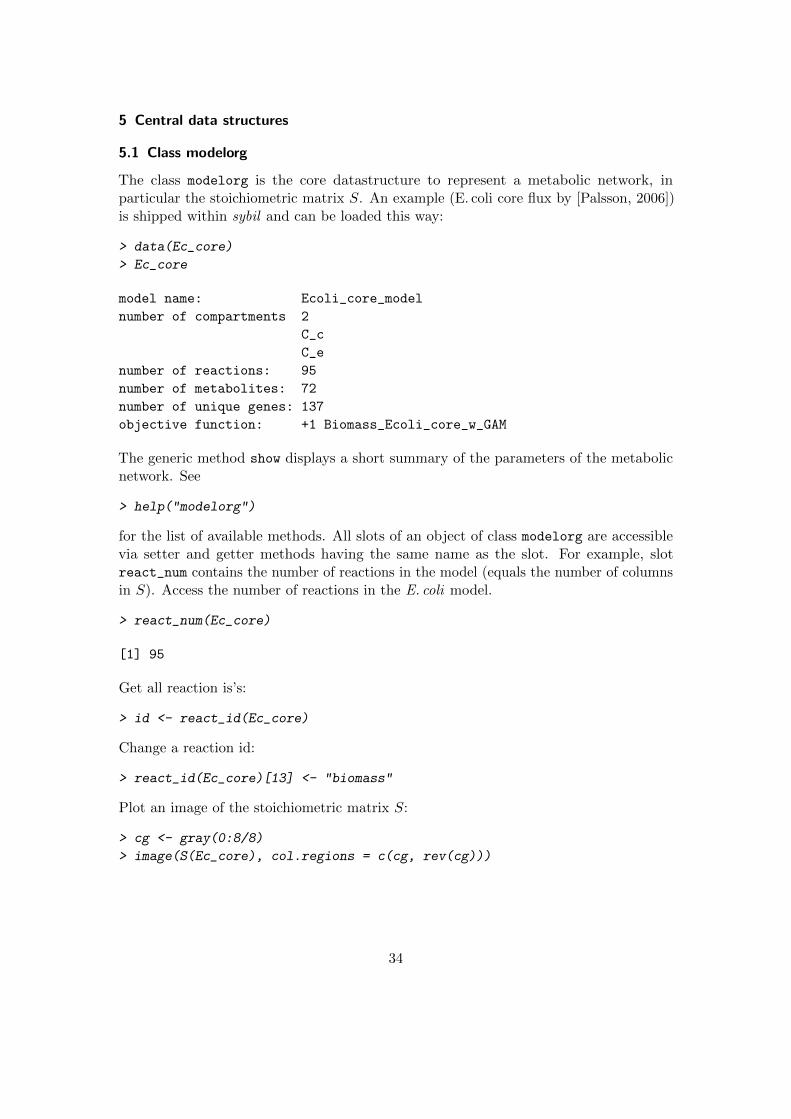
Plot an image of the stoichiometric matrix S:

> cg <- gray(0:8/8)

> image(S(Ec_core), col.regions = c(cg, rev(cg)))

34

Dimensions: 72 x 95Column

Row

20

40

60

20 40 60 80

−60

−40

−20

0

20

40

60

Matrices in objects of class modelorg are stored in formats provided by the Matrix -package9.

Objects of class modelorg can easily be created. Sources are common file formats liketab delimited files from the BiGG database [Schellenberger et al., 2010]10 or SBML files(with package sybilSBML3). See section 3 on page 2 about supported file formats andtheir description. Read a reaction list generated from the BiGG database:

> mod <- readTSVmod(reactList = "reactionList.txt")

Here, "reactionList.txt" is an from BiGG database exported reaction list. Usually,these files do neither contain an objective function, nor upper and lower bounds on thereaction rates. They need to be added to the returned object of class modelorg usingthe methods obj_coef<-, lowbnd<- and uppbnd<-, or by adding the columns obj_coef,lowbnd and uppbnd to the input file.

35

show()mod_obj()getFluxDist()checkStat()checkOptSol()!uxes()n!uxes()length()plot()

mod_id: character 1mod_key: character 1solver: character 1method: character 1algorithm: character 1num_of_prob: integer 1lp_num_cols: integer 1lp_num_rows: integer 1lp_obj: numeric 1..*lp_ok: integer 1..*lp_stat: integer 1..*lp_dir: character 1..*obj_coef: numeric 1..*obj_func: character 1!dind: integer 1..*!uxdist: !uxDistribution 1alg_par: list 1..*

optsol (VIRTUAL)

lethal()deleted()[

chlb: numeric 1..*chub: numeric 1..*dels: matrix 1

!uxdel

plot()

ctrlr: reactId 1ctrl!: numeric 1..*

robAna

plot()plotRangeVar()minSol()maxSol()blReact()

react: reactId 1!uxVar

deleted()

!uxdels: list 1..*hasE"ect: logical 1..*

genedeloptimizeProbpreProc: ppProc 1postProc: ppProc 1

plot()

ctrl!m: matrix 1redCosts: matrix 1

phpp

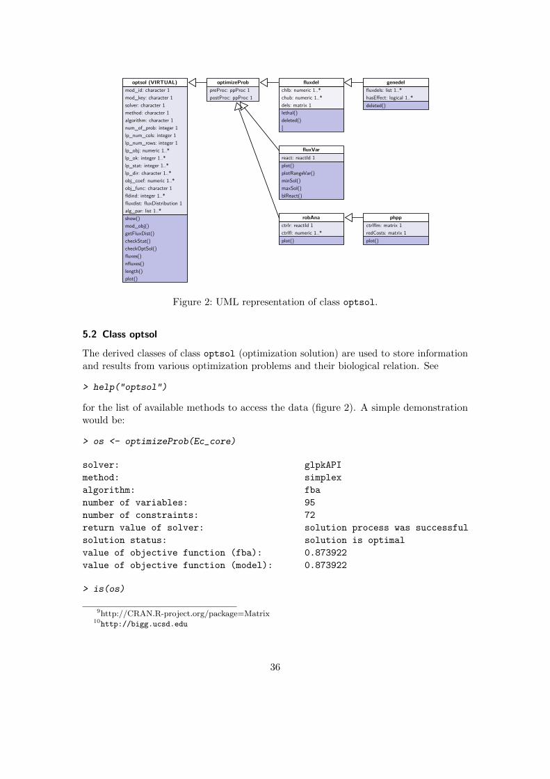
Figure 2: UML representation of class optsol.

5.2 Class optsol

The derived classes of class optsol (optimization solution) are used to store informationand results from various optimization problems and their biological relation. See

> help("optsol")

for the list of available methods to access the data (figure 2). A simple demonstrationwould be:

> os <- optimizeProb(Ec_core)

solver: glpkAPI

method: simplex

algorithm: fba







> is(os)

9http://CRAN.R-project.org/package=Matrix10http://bigg.ucsd.edu

36

http://bigg.ucsd.edu

[1] "optsol_optimizeProb" "optsol"

Retrieve objective value.

> lp_obj(os)

[1] 0.8739215

Retrieve flux distribution.

> getFluxDist(os)

1 2 3 4 5

1.250555e-12 1.364242e-12 -1.023182e-12 6.007250e+00 6.007250e+00

6 7 8 9 10

-1.023182e-12 4.547474e-13 5.064376e+00 0.000000e+00 0.000000e+00

11 12 13 14 15

8.390000e+00 4.551401e+01 8.739215e-01 -2.280983e+01 6.007250e+00

16 17 18 19 20

4.359899e+01 -6.821210e-13 1.471614e+01 0.000000e+00 0.000000e+00

21 22 23 24 25

0.000000e+00 0.000000e+00 2.280983e+01 0.000000e+00 0.000000e+00

26 27 28 29 30

0.000000e+00 0.000000e+00 -1.000000e+01 0.000000e+00 0.000000e+00

31 32 33 34 35

1.753087e+01 2.917583e+01 0.000000e+00 0.000000e+00 -4.765319e+00

36 37 38 39 40

-2.179949e+01 -3.214895e+00 0.000000e+00 0.000000e+00 7.477382e+00

41 42 43 44 45

0.000000e+00 0.000000e+00 0.000000e+00 0.000000e+00 0.000000e+00

46 47 48 49 50

5.064376e+00 0.000000e+00 4.959985e+00 1.602353e+01 1.000000e+01

51 52 53 54 55

2.234617e-01 0.000000e+00 -4.541857e+00 0.000000e+00 0.000000e+00

56 57 58 59 60

0.000000e+00 4.959985e+00 -2.917583e+01 6.007250e+00 0.000000e+00

61 62 63 64 65

-6.821210e-13 -3.248195e-13 0.000000e+00 5.064376e+00 0.000000e+00

66 67 68 69 70

0.000000e+00 3.853461e+01 0.000000e+00 4.765319e+00 2.179949e+01

71 72 73 74 75

9.282533e+00 7.477382e+00 0.000000e+00 4.860861e+00 -1.602353e+01

76 77 78 79 80

4.959985e+00 -1.471614e+01 3.214895e+00 2.504309e+00 0.000000e+00

81 82 83 84 85

37

initialize()dim()...

oobj: pointerToProb 1solver: character 1method: character 1probType: character 1

optObj (VIRTUAL)

initProb()setSolverParm()loadLPprob()solveLp()getObjVal()getSolStat()...

glpkAPIinitProb()setSolverParm()loadLPprob()solveLp()getObjVal()getSolStat()...

cplexAPIinitProb()setSolverParm()loadLPprob()solveLp()getObjVal()getSolStat()...

clpAPIinitProb()setSolverParm()loadLPprob()solveLp()getObjVal()getSolStat()...

lpSolveAPI

initProb()setSolverParm()loadLPprob()solveLp()getObjVal()getSolStat()...

grb: character 1sybilGUROBI

Figure 3: UML representation of class optObj.

0.000000e+00 -2.046363e-12 1.758177e+00 0.000000e+00 2.678482e+00

86 87 88 89 90

-2.281503e+00 8.881784e-16 0.000000e+00 5.064376e+00 -5.064376e+00

91 92 93 94 95

1.496984e+00 0.000000e+00 1.496984e+00 1.181498e+00 7.477382e+00

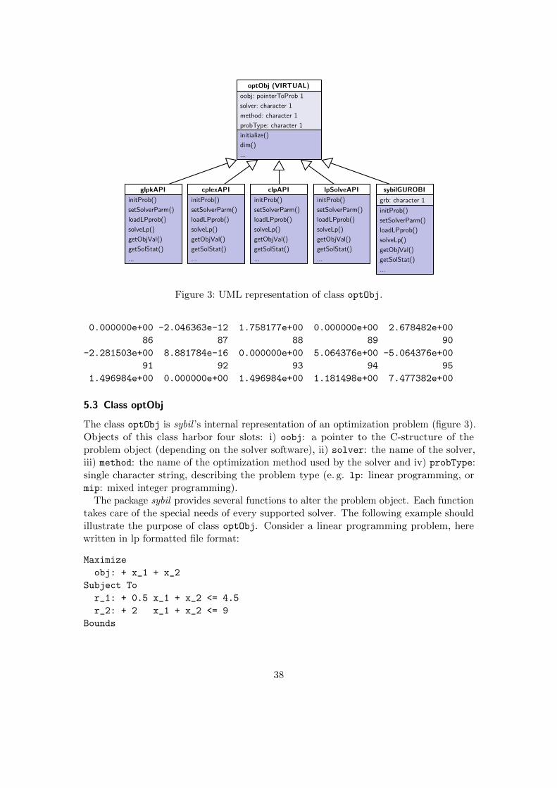
5.3 Class optObj

The class optObj is sybil ’s internal representation of an optimization problem (figure 3).Objects of this class harbor four slots: i) oobj: a pointer to the C-structure of theproblem object (depending on the solver software), ii) solver: the name of the solver,iii) method: the name of the optimization method used by the solver and iv) probType:single character string, describing the problem type (e. g. lp: linear programming, ormip: mixed integer programming).

The package sybil provides several functions to alter the problem object. Each functiontakes care of the special needs of every supported solver. The following example shouldillustrate the purpose of class optObj. Consider a linear programming problem, herewritten in lp formatted file format:

Maximize

obj: + x_1 + x_2

Subject To

r_1: + 0.5 x_1 + x_2 <= 4.5

r_2: + 2 x_1 + x_2 <= 9

Bounds

38

startsolver: character

method: characterpType: character

new("solver", solver,method, pType)result: optObjstop

checkDefaultMethod(solver,method, pType)

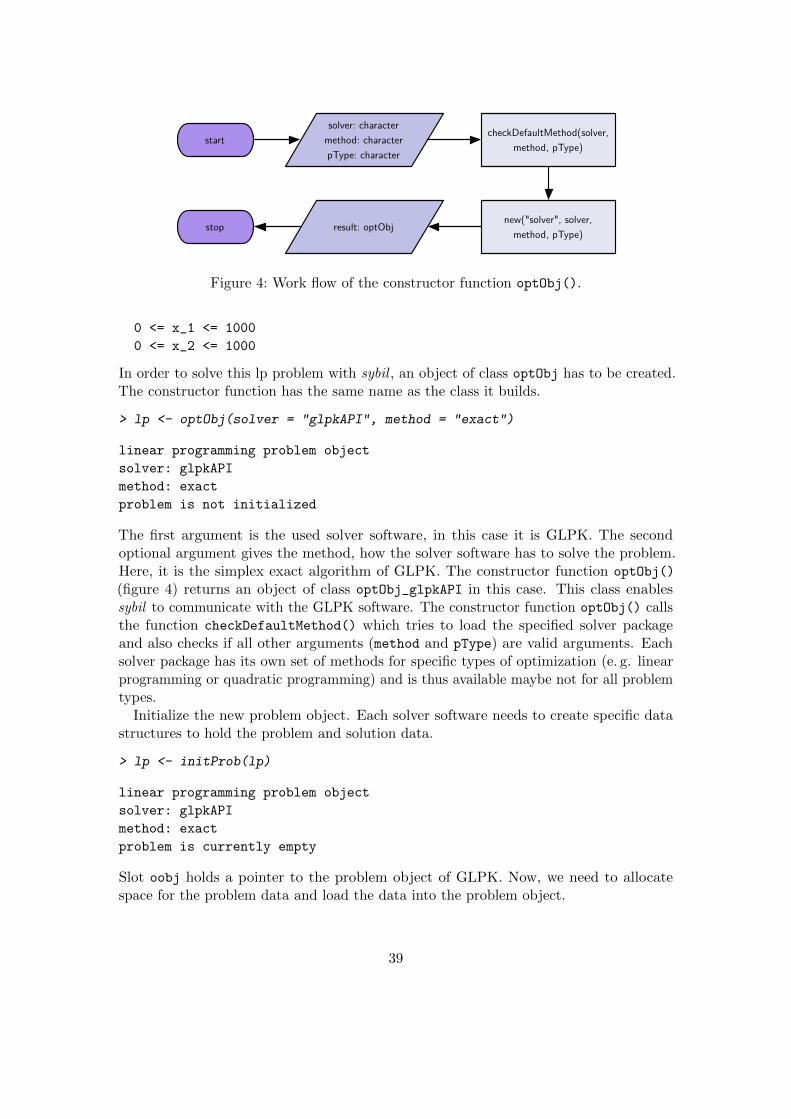
Figure 4: Work flow of the constructor function optObj().

0 <= x_1 <= 1000

0 <= x_2 <= 1000

In order to solve this lp problem with sybil , an object of class optObj has to be created.The constructor function has the same name as the class it builds.

> lp <- optObj(solver = "glpkAPI", method = "exact")

linear programming problem object

solver: glpkAPI

method: exact

problem is not initialized

The first argument is the used solver software, in this case it is GLPK. The secondoptional argument gives the method, how the solver software has to solve the problem.Here, it is the simplex exact algorithm of GLPK. The constructor function optObj()

(figure 4) returns an object of class optObj_glpkAPI in this case. This class enablessybil to communicate with the GLPK software. The constructor function optObj() callsthe function checkDefaultMethod() which tries to load the specified solver packageand also checks if all other arguments (method and pType) are valid arguments. Eachsolver package has its own set of methods for specific types of optimization (e. g. linearprogramming or quadratic programming) and is thus available maybe not for all problemtypes.

Initialize the new problem object. Each solver software needs to create specific datastructures to hold the problem and solution data.

> lp <- initProb(lp)


solver: glpkAPI

method: exact

problem is currently empty

Slot oobj holds a pointer to the problem object of GLPK. Now, we need to allocatespace for the problem data and load the data into the problem object.

39

> cm <- Matrix(c(0.5, 2, 1, 1), nrow = 2)

> loadLPprob(lp, nCols = 2, nRows = 2, mat = cm,

+ lb = c(0, 0), ub = rep(1000, 2), obj = c(1, 1),

+ rlb = c(0, 0), rub = c(4.5, 9), rtype = c("U", "U"),

+ lpdir = "max")

The first command generates the constraint matrix in sparse format (see also documenta-tion in package Matrix ). The second command loads the problem data into the problemobject.

> lp


solver: glpkAPI

method: exact

problem has 2 variables and 2 constraints

All data are now set in the problem object, so it can be solved.

> status <- solveLp(lp)

[1] 0

Translate the status code in a text string.

> getMeanReturn(code = status, solver = solver(lp))

[1] "solution process was successful"

Check the solution status.

> status <- getSolStat(lp)

> getMeanStatus(code = status, solver = solver(lp))

[1] "solution is optimal"

Retrieve the value of the objective function and the values of the variables after opti-mization.

> getObjVal(lp)

[1] 6

> getFluxDist(lp)

[1] 3 3

Get the reduced costs.

40

initialize()optimizeProb()applyChanges()resetChanges()...

problem: optObj 1algorithm: character 1nr: integer 1nc: integer 1!dind: integer 1..*alg_par: list 1..*

sysBiolAlg (VIRTUAL)

initialize()fba (LP)

initialize()lmoma (LP)

initialize()moma (QP)

initialize()applyChanges()resetChanges()

wu: numeric 1wl: numeric 1fnr: integer 1fnc: integer 1

room (MILP)initialize()...

???

initialize()changeMaxObj()

maxobj: numeric 1..*mtf (LP)

initialize()fv (LP)

Figure 5: UML representation of class sysBiolAlg.

> getRedCosts(lp)

[1] 0 0

Delete problem object and free all memory allocated by the solver software.

> delProb(lp)

> lp


solver: glpkAPI

method: exact

problem is not initialized

5.4 Class sysBiolAlg

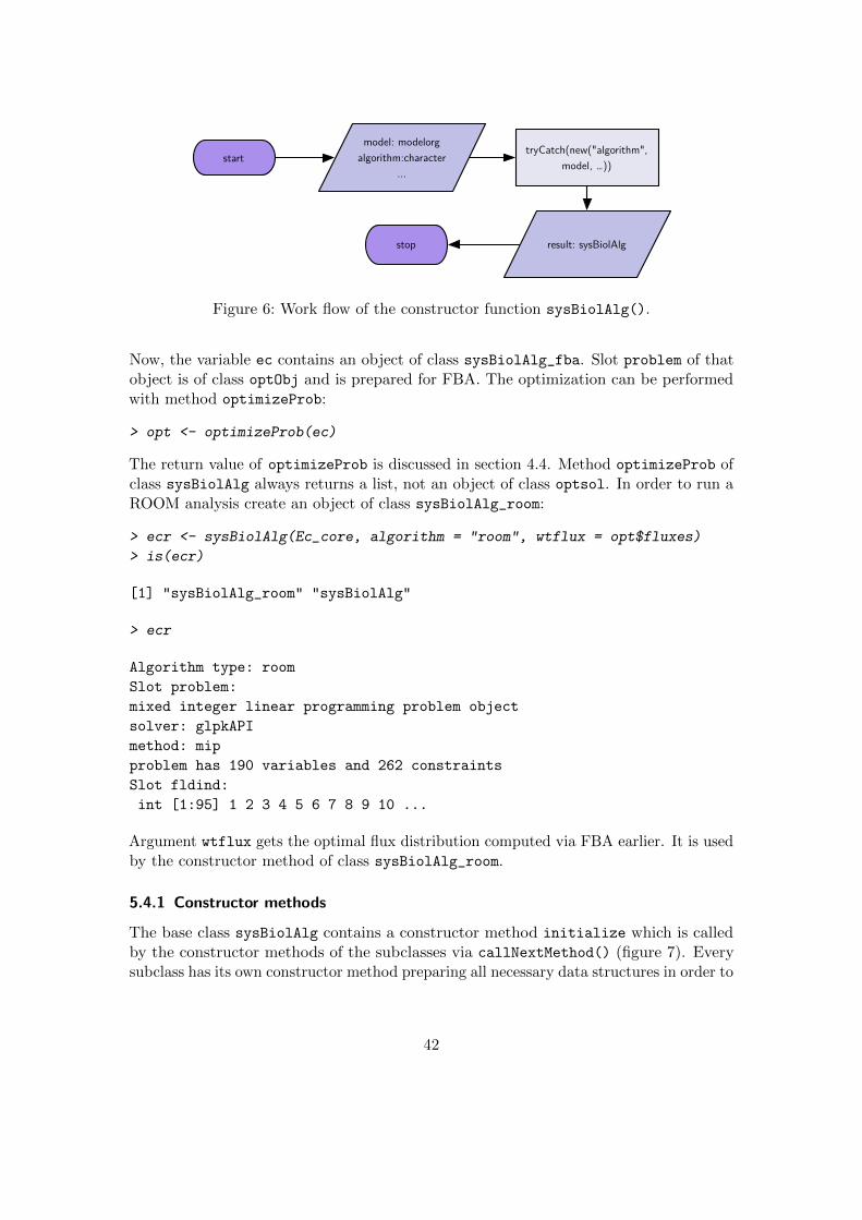
The class sysBiolAlg holds objects of class optObj which are prepared for a particularkind of algorithm, e. g. FBA, MOMA or ROOM (figure 5). Class optObj takes care ofthe communication between sybil and the solver software. Class sysBiolAlg insteadis responsible for the algorithm used to analyze a metabolic network. The constructorfunction sysBiolalg() (figure 6) gets at least two arguments: 1. an object of classmodelorg (section 5.1) and 2. a single character string indicating the name of the desiredalgorithm. Further arguments are passed through argument ... to the correspondingconstructor of the class extending class sysBiolAlg. The base class sysBiolAlg isvirtual, no objects can be created from that class directly. The constructor functionbuilds an instance of a class extending the base class:

> ec <- sysBiolAlg(Ec_core, algorithm = "fba")

> is(ec)

[1] "sysBiolAlg_fba" "sysBiolAlg"

41

startmodel: modelorg

algorithm:character...

tryCatch(new("algorithm", model, …))

result: sysBiolAlgstop

Figure 6: Work flow of the constructor function sysBiolAlg().

Now, the variable ec contains an object of class sysBiolAlg_fba. Slot problem of thatobject is of class optObj and is prepared for FBA. The optimization can be performedwith method optimizeProb:

> opt <- optimizeProb(ec)

The return value of optimizeProb is discussed in section 4.4. Method optimizeProb ofclass sysBiolAlg always returns a list, not an object of class optsol. In order to run aROOM analysis create an object of class sysBiolAlg_room:

> ecr <- sysBiolAlg(Ec_core, algorithm = "room", wtflux = opt$fluxes)

> is(ecr)

[1] "sysBiolAlg_room" "sysBiolAlg"

> ecr

Algorithm type: room

Slot problem:

mixed integer linear programming problem object

solver: glpkAPI

method: mip

problem has 190 variables and 262 constraints

Slot fldind:

int [1:95] 1 2 3 4 5 6 7 8 9 10 ...

Argument wtflux gets the optimal flux distribution computed via FBA earlier. It is usedby the constructor method of class sysBiolAlg_room.

5.4.1 Constructor methods

The base class sysBiolAlg contains a constructor method initialize which is calledby the constructor methods of the subclasses via callNextMethod() (figure 7). Everysubclass has its own constructor method preparing all necessary data structures in order to

42

initialize, sysBiolAlg-method

start

.Object,model: modelorg

...

stop

generate data structures corresponding to the used algorithm (constraint matrix,

right hand side, ...)

generate an empty problem object:lp ← optObj(solver, method, pType)

initialize problem object:initProb(lp, nRows, nCols)

set solver parameterssetSolverParm(lp, list of parameters)

load data into the problem objectloadLPprob(lp, further data structures)

set data part of .Object.Object@problem ← lp

.Object@problem ← "algorithm"...

additional modi"cations if required

validate problem object

result: sysBiolAlg

Figure 7: Work flow of the constructor methods of classes extending class sysBiolAlg.The gray shaded part is done by the constructor method or the base class.

call the constructor of the base class. For example, for the ROOM algorithm, a “wild type”flux distribution is required (argument wtflux in the example above). The constructor ofclass sysBiolAlg_room generates all data structures to build the optimization problem,e. g. the constraint matrix, objective coefficients, right hand side, . . . It passes all thesedata to the constructor of sysBiolAlg via a call to callNextMethod(). This constructorgenerates the object of class optObj while taking care on solver software specific details.

5.4.2 New algorithms

In order to extend the functionality of sybil with new algorithms, a new class describingthat algorithm is required. The function promptSysBiolAlg() generates a skeletalstructure of a new class definition and a corresponding constructor method. To implementan algorithm named “foo”, run

> promptSysBiolAlg(algorithm = "foo")

which generates a file sysBiolAlg_fooClass.R containing the new class definition. Theclass sysBiolAlg_foo will extend class sysBiolAlg directly and will not add any slotsto the class. Additionally, an unfinished method initialize is included. Here it is

43

necessary to generate the data structures required by the new algorithm. There arecomments in the skeletal structure guiding through the process.

44

References

S. A. Becker et al. Quantitative prediction of cellular metabolism with constraint-basedmodels: the COBRA Toolbox. Nat Protoc, 2(3):727–738, 2007. doi: 10.1038/nprot.2007.99.

J. S. Edwards, R. U. Ibarra, and B. Ø. Palsson. In silico predictions of Escherichia colimetabolic capabilities are consistent with experimental data. Nat Biotechnol, 19(2):125–130, Feb 2001. doi: 10.1038/84379.

J. S. Edwards, M. Covert, and B. Ø. Palsson. Metabolic modelling of microbes: theflux-balance approach. Environ Microbiol, 4(3):133–140, Mar 2002a.

J. S. Edwards, R. Ramakrishna, and B. Ø. Palsson. Characterizing the metabolicphenotype: a phenotype phase plane analysis. Biotechnol Bioeng, 77(1):27–36, Jan2002b.

R. Mahadevan and C. H. Schilling. The effects of alternate optimal solutions in constraint-based genome-scale metabolic models. Metab Eng, 5(4):264–276, Oct 2003.

J. D. Orth, R. M. T. Fleming, and B. Ø. Palsson. Reconstruction and use of microbialmetabolic networks: the core Escherichia coli metabolic model as an educational guide.EcoSal Chapter 10.2.1, 2010a.

J. D. Orth, I. Thiele, and B. Ø. Palsson. What is flux balance analysis? Nat Biotechnol,28(3):245–248, Mar 2010b. doi: 10.1038/nbt.1614.

B. Ø. Palsson. Systems Biology: Properties of Recontructed Networks. CambridgeUniversity Press, 2006.

J. Schellenberger, J. O. Park, T. M. Conrad, and B. Ø. Palsson. BiGG: a biochemicalgenetic and genomic knowledgebase of large scale metabolic reconstructions. BMCBioinformatics, 11:213, 2010. doi: 10.1186/1471-2105-11-213.

J. Schellenberger, R. Que, R. M. T. Fleming, I. Thiele, J. D. Orth, A. M. Feist, D. C.Zielinski, A. Bordbar, N. E. Lewis, S. Rahmanian, J. Kang, D. R. Hyduke, and B. Ø.Palsson. Quantitative prediction of cellular metabolism with constraint-based models:the COBRA Toolbox v2.0. Nat Protoc, 6(9):1290–1307, 2011. doi: 10.1038/nprot.2011.308.

D. Segre et al. Analysis of optimality in natural and perturbed metabolic networks. ProcNatl Acad Sci U S A, 99(23):15112–15117, Nov 2002. doi: 10.1073/pnas.232349399.

T. Shlomi, O. Berkman, and E. Ruppin. Regulatory on/off minimization of metabolicflux changes after genetic perturbations. Proc Natl Acad Sci U S A, 102(21):7695–7700,May 2005. doi: 10.1073/pnas.0406346102.

45

Documents

sybil Efficient Constrained Based Modelling in R · The R-package sybil is a Systems Biology Library for R, implementing algorithms for constraint based analysis of metabolic networks