SWUTC/11/161025-1 DEVELOPMENT OF RELIABLE PAVEMENT …

1. Report No.

SWUTC/11/161025-1 2. Government Accession No.

3. Recipient's Catalog No.

4. Title and Subtitle

DEVELOPMENT OF RELIABLE PAVEMENT MODELS 5. Report Date

May 2011 6. Performing Organization Code

7. Author(s)

José Pablo Aguiar-Moya, Jorge Prozzi 8. Performing Organization Report No.

161025-1 9. Performing Organization Name and Address

Center for Transportation Research University of Texas at Austin 1616 Guadalupe Street, Suite 4.200 Austin, Texas 78701

10. Work Unit No. (TRAIS)

11. Contract or Grant No.

10727

12. Sponsoring Agency Name and Address

Southwest Region University Transportation Center Texas Transportation Institute Texas A&M University System College Station, Texas 77843-3135

13. Type of Report and Period Covered

14. Sponsoring Agency Code

15. Supplementary Notes

Supported by general revenues from the State of Texas. 16. Abstract

The current report proposes a framework for estimating the reliability of a given pavement structure as analyzed by the Mechanistic-Empirical Pavement Design Guide (MEPDG). The methodology proposes using a previously fit response surface, in place of the time-demanding implicit limit state functions used within the MEPDG, in combination with an analytical approach to estimating reliability using First-Order and Second-Order Reliability Methods (FORM and SORM). Additionally, in order to assess the accuracy of the FORM and SORM reliability estimates, Monte Carlo simulations are also performed. A case study based on a three-layered pavement structure is used to demonstrate the methodology. Several pavement design variables are treated as random; these include HMA and base layer thicknesses, base and subgrade modulus, and HMA layer binder and air void content. Information on the variability and correlation between these variables are obtained from the Long-Term Pavement Performance (LTPP) program. Response surfaces for limit states dealing with HMA rutting failure are fit using several runs of the MEPDG based on a factorial design of combinations among the aforementioned random variables, as well as traffic, structural, and climatic considerations. These response surfaces are then used to analyze the reliability of the given pavement structure. Using the second moment and simulation techniques, it was found that on average the reliability estimate by the MEPDG is very conservative. Additionally, the validity of the methodology is verified by means of direct simulation using the MEPDG. Finally, recommendations on fitting the response surface are provided to ensure the applicability of the methodology. 17. Key Words

Mechanistic-Empirical Pavement Design Guide (MEPDG); First-Order and Second-Order Reliability Methods (FORM and SORM); Pavement Structure; Pavement Response

18. Distribution Statement

No restrictions. This document is available to the public through NTIS: National Technical Information Service 5285 Port Royal Road Springfield, Virginia 22161

19. Security Classif.(of this report)

Unclassified 20. Security Classif.(of this page)

Unclassified 21. No. of Pages

150

22. Price

Technical Report Documentation Page

Form DOT F 1700.7 (8-72) Reproduction of completed page authorized

ii

iii

Development of Reliable Pavement Models

By

José Pablo Aguiar-Moya

Jorge Prozzi

Research Report SWUTC/11/161025-1

Southwest Region University Transportation Center Center for Transportation Research

University of Texas at Austin Austin, Texas 78712

May 2011

iv

v

ABSTRACT

The current report proposes a framework for estimating the reliability of a given

pavement structure as analyzed by the Mechanistic-Empirical Pavement Design Guide

(MEPDG). The methodology proposes using a previously fit response surface, in place of the

time-demanding implicit limit state functions used within the MEPDG, in combination with an

analytical approach to estimating reliability using First-Order and Second-Order Reliability

Methods (FORM and SORM). Additionally, in order to assess the accuracy of the FORM and

SORM reliability estimates, Monte Carlo simulations are also performed.

A case study based on a three-layered pavement structure is used to demonstrate the

methodology. Several pavement design variables are treated as random; these include HMA and

base layer thicknesses, base and subgrade modulus, and HMA layer binder and air void content.

Information on the variability and correlation between these variables are obtained from the

Long-Term Pavement Performance (LTPP) program.

Response surfaces for limit states dealing with HMA rutting failure are fit using several

runs of the MEPDG based on a factorial design of combinations among the aforementioned

random variables, as well as traffic, structural, and climatic considerations. These response

surfaces are then used to analyze the reliability of the given pavement structure.

Using the second moment and simulation techniques, it was found that on average the

reliability estimate by the MEPDG is very conservative. Additionally, the validity of the

methodology is verified by means of direct simulation using the MEPDG. Finally,

recommendations on fitting the response surface are provided to ensure the applicability of the

methodology.

vi

EXECUTIVE SUMMARY

As the cost of designing and building new highway pavements increases and the number of new

construction and major rehabilitation projects decreases, the importance of ensuring that a given

pavement design performs as expected in the field becomes vital. To address this issue in other

fields of civil engineering, reliability analysis has been used extensively. However, in the case of

pavement structural design, the reliability component is usually neglected or overly simplified.

To address this need, the current research project proposes a framework for estimating the

reliability of a given pavement structure regardless of the pavement design or analysis procedure

that is being used.

The framework is applied with the Mechanistic-Empirical Pavement Design Guide (MEPDG)

and failure is considered as a function of rutting of the hot-mix asphalt (HMA) layer. The

proposed methodology consists of fitting a response surface, in place of the time-demanding

implicit limit state functions used within the MEPDG, in combination with an analytical

approach to estimating reliability using second moment techniques: First-Order and Second-

Order Reliability Methods (FORM and SORM) and simulation techniques: Monte Carlo and

Latin Hypercube Simulation.

In order to demonstrate the methodology, a three-layered pavement structure is selected

consisting of a hot-mix asphalt (HMA) surface, a base layer, and subgrade. Several pavement

design variables are treated as random; these include HMA and base layer thicknesses, base and

subgrade modulus, and HMA layer binder and air void content. Information on the variability

and correlation between these variables are obtained from the Long-Term Pavement

Performance (LTPP) program, and likely distributions, coefficients of variation, and correlation

between the variables are estimated. Additionally, several scenarios are defined to account for

climatic differences (cool, warm, and hot climatic regions), truck traffic distributions (mostly

consisting of single unit trucks versus mostly consisting of single trailer trucks), and the

thickness of the HMA layer (thick versus thin).

vii

First and second order polynomial HMA rutting failure response surfaces with interaction terms

are fit by running the MEPDG under a full factorial experimental design consisting of 3 levels of

the aforementioned design variables. These response surfaces are then used to analyze the

reliability of the given pavement structures under the different scenarios. Additionally, in order

to check for the accuracy of the proposed framework, direct simulation using the MEPDG was

performed for the different scenarios. Very small differences were found between the estimates

based on response surfaces and direct simulation using the MEPDG, confirming the accurateness

of the proposed procedure.

Finally, sensitivity analysis on the number of MEPDG runs required to fit the response surfaces

was performed and it was identified that reducing the experimental design by one level still

results in response surfaces that properly fit the MEPDG, ensuring the applicability of the

method for practical applications by greatly reducing the number of runs of the MEPDG required

to fit a given response surface.

viii

ix

TABLE OF CONTENTS

Abstract ................................................................................................................................ v

Executive Summary ............................................................................................................ vi

List of Figures .................................................................................................................... vii

List of Tables……………………………………………………………………………..xiv

Disclaimer and Acknowledgements…………………………………………………… xvii

Chapter 1: Motivation…………………………………………………………………… . 1

1.1. Research Objectives ............................................................................................ 2

1.2. Report Layout ...................................................................................................... 3

Chapter 2: Literature Review ............................................................................................. 7

2.1. Structural Pavement Design ................................................................................ 7

2.1.1. AASHTO Guide for Design of Pavement Structures .............................. 8

2.1.2. Mechanistic-Empirical Pavement Design Guide (MEPDG) ................. 10

2.2. Factors Affecting Pavement Design .................................................................. 11

2.2.1. Traffic .................................................................................................... 11

2.2.2. Environmental Conditions ..................................................................... 12

2.2.3. Structure and Materials .......................................................................... 13

2.2.4. Interaction between design variables ..................................................... 14

2.3. Reliability in Current Pavement Design Methodologies ................................... 15

Chapter 3: Reliability........................................................................................................ 17

3.1. Reliability in the AASHTO Guide .................................................................... 18

3.2. Reliability in the MEPDG ................................................................................. 20

3.3. Uncertainties in the Estimation of Reliability ................................................... 24

3.4. Reliability by Means of Simulation Techniques ............................................... 25

3.5. Reliability by Means of Second Moment Techniques ....................................... 28

3.5.1. First Order Reliability Method (FORM) ............................................... 28

3.5.2. Second Order Reliability Method (SORM) ........................................... 30

x

3.6. Response Surface Approach to Reliability ........................................................ 33

Chapter 4: Variability in Pavement Design ...................................................................... 39

4.1. The Long Term Pavement Performance (LTPP) Database ............................... 45

4.2. Goodness-of-Fit Tests For Variable Distributions ............................................ 47

4.3. Variability in Pavement Layer Thickness ......................................................... 48

4.4. Variability in Asphalt Binder Content ............................................................... 54

4.5. Variability in Air Void Content ......................................................................... 56

4.6. Variability in Modulus of Unbound Material Layers ........................................ 58

4.7. Variability in Modulus of HMA Layers ............................................................ 60

4.8. Variability Summary ......................................................................................... 62

Chapter 5: Reliability Analysis using the MEPDG .......................................................... 65

5.1. Selection of Random Variables ......................................................................... 65

5.2. Definition of Pavement Sections to be Analyzed .............................................. 66

5.2.1. Traffic Loading ...................................................................................... 68

5.3. Development of 1-Degree Response Surfaces for Rutting Performance .......... 73

5.4. FORM Analysis Based on 1-Degree Response Surface .................................... 79

5.5. Simulation Analysis based on 1-Degree Response Surface .............................. 82

Chapter 6: Correction in Reliability Estimates Due to Curvature .................................... 85

6.1. Development of 2-Degree Response Surfaces With Interaction Terms for Rutting

Performance ..................................................................................................... 85

6.2. FORM and SORM Analysis Based on 2-Degree Response Surface With Interaction

Terms ............................................................................................................... 89

6.3. Elasticity Analysis ............................................................................................. 92

6.4. Simulation Analysis based on 2-Degree Response Surface With Interaction Terms

......................................................................................................................... 95

Chapter 7: Direct MEPDG Simulation ............................................................................. 99

7.1. Error Associated with the Simulation .............................................................. 100

xi

7.2. Direct Simulation using the MEPDG .............................................................. 100

7.3. Change in Reliability with Time ..................................................................... 103

Chapter 8: Sensitivity to Response Surface .................................................................... 107

8.1. Development of Reduced 1-Degree Response Surfaces for Rutting Performance

....................................................................................................................... 108

8.2. FORM Analysis Based on Reduced 1-Degree Response Surface ................... 110

8.3. Simulation Analysis based on Reduced 1-Degree Response Surface ............. 113

Chapter 9: Conclusions ................................................................................................... 117

9.1. Summary and Concluding Remarks ................................................................ 117

References ....................................................................................................................... 123

Appendix 1: Normality Goodness-of-Fit Tests .............................................................. 129

A1.1. Skewness-Kurtosis Test ................................................................................ 129

A1.1.1. Skewness........................................................................................... 129

A1.1.2. Kurtosis ............................................................................................. 130

A1.1.3. Skewness and Kurtosis Combined Statistic ...................................... 131

A1.2. Shapiro-Francia Test ..................................................................................... 131

xii

LIST OF FIGURES

Figure 2.1: Schematic of processes involved in the MEPDG (from NCHRP, 2004). .... 10

Figure 3.1: Conceptualization of Reliability Index. ........................................................ 30

Figure 3.2: Comparison of relative error from reliability estimates based on FORM and

SORM to different Monte Carlo simulation estimates for cracking on steam

generator tubing (from Cizelj et al., 1994). .................................................. 32

Figure 3.3: Pavement failure probabilities by Second Moment (and higher order moments)

and crude Monte Carlo simulation (from Zhang and Damnjanović, 2006). 33

Figure 3.4: Comparison of direct simulation to simulation based on response surfaces for

SDOF systems (from Yao and Wen, 1996). ................................................. 51

Figure 3.5: Comparison of direct simulation (FE) to simulation based on response surfaces

(RS) for soil slopes (from Wong, 1985). ...................................................... 36

Figure 4.1: Effect of HMA layer thickness on rutting and roughness according to the

MEPDG. ....................................................................................................... 42

Figure 4.2: Effect of base thickness on rutting and roughness according to the MEPDG.42

Figure 4.3: Effect of binder content on rutting and roughness according to the MEPDG.43

Figure 4.4: Effect of air voids on rutting and roughness according to the MEPDG. ...... 43

Figure 4.5: Effect of base modulus on rutting and roughness according to the MEPDG.44

Figure 4.6: Effect of subgrade modulus on rutting and roughness according to the MEPDG.

...................................................................................................................... 44

Figure 4.7: Location of LTPP GPS and SPS pavement sections (from http://www.ltpp-

products.com). .............................................................................................. 46

Figure 4.8: HMA surface layer thickness distribution for LTPP section 48-0113 (under right

wheel-path). .................................................................................................. 50

Figure 4.9: Binder course layer thickness distribution for LTPP section 48-0116 (under lane

centerline). .................................................................................................... 52

Figure 4.10: Normal probability plot for HMA Binder course layer thickness for LTPP

section 48-0116 (under lane centerline). ...................................................... 53

Figure 4.11: Asphalt binder content distribution for LTPP section 29-0962. ................... 55

xiii

Figure 4.12: Air void content distribution for LTPP section 26-0114. ............................. 57

Figure 4.13: Resilient modulus distribution for a subgrade layer with mean 13,200 psi. 59

Figure 4.14: Resilient modulus distribution for a HMA layer with mean 750 ksi............ 62

Figure 5.1: Locations of climatic regions to be analyzed as part of the reliability analysis.

...................................................................................................................... 67

Figure 5.2: Truck Traffic Classes included in the MEPDG (from NCHRP, 2004). ....... 69

Figure 5.3: Type 2 Truck Traffic Classification. ............................................................ 69

Figure 5.4: Type 12 Truck Traffic Classification. .......................................................... 70

Figure 5.5: Effect of traffic on rutting of the HMA layer (4.5 in HMA layer, TTC 2). . 71

Figure 5.6: Effect of traffic on rutting of the HMA layer (4.5 in HMA layer,

TTC 12). ....................................................................................................... 71

Figure 5.7: Effect of traffic on rutting of the HMA layer (10.0 in HMA layer,

TTC 2). ......................................................................................................... 72

Figure 5.8: Effect of traffic on rutting of the HMA layer (10.0 in HMA layer, TTC

12). ................................................................................................................ 72

Figure 5.9: Effect of air void content on rutting of a 10.0 in HMA layer in a Warm Climatic

Region (TTC 2). ........................................................................................... 74

Figure 5.10: Effect of asphalt binder content on rutting of a 4.5 in HMA layer in a Hot

Climatic Region (TTC 2). ............................................................................. 75

Figure 5.11: Effect of base modulus on rutting of a 4.5 in HMA layer in a Hot Climatic

Region (TTC 12). ......................................................................................... 76

Figure 7.1: Change in reliability with time. .................................................................. 104

xiv

LIST OF TABLES

Table 2.1: Minimum reliability levels recommended for pavement structures (from

AASHTO, 1993). .......................................................................................... 15

Table 3.1: Computed statistical parameters for each category of HMA layer rutting

(NCHRP, 2004). ........................................................................................... 22

Table 4.1: Coefficient of variation of pavement layer thickness. .................................. 54

Table 4.2: Coefficient of variation of unbound layer resilient modulus. ....................... 60

Table 5.1: Pavement design variables to be treated as random parameters. .................. 66

Table 5.2: Mean and standard deviation for random design variables. ......................... 68

Table 5.3: Critical AADTT values to ensure 0.25 in of rutting on the HMA layer. ...... 73

Table 5.4: Parameter estimates for rutting of HMA layer in Cool Climatic Region. .... 77

Table 5.5: Parameter estimates for rutting of HMA layer in Warm Climatic Region. .. 78

Table 5.6: Parameter estimates for rutting of HMA layer in Hot Climatic Region. ...... 78

Table 5.7: Reliability Analysis based on FORM for HMA layers in Cool Climatic Region

(1-degree response surface). ......................................................................... 80

Table 5.8: Reliability Analysis based on FORM for HMA layers in Warm Climatic Region


Table 5.9: Reliability Analysis based on FORM for HMA layers in Hot Climatic Region


Table 5.10: Reliability Analysis based on simulation for HMA layers in Cool Climatic

Region (1-degree response surface). ............................................................ 83

Table 5.11: Reliability Analysis based on simulation for HMA layers in Warm Climatic


Table 5.12: Reliability Analysis based on simulation for HMA layers in Hot Climatic


Table 6.1: Parameter estimates for rutting of HMA layer in Cool Climatic Region. .... 86

Table 6.2: Parameter estimates for rutting of HMA layer in Warm Climatic Region. .. 87

Table 6.3: Parameter estimates for rutting of HMA layer in Hot Climatic Region. ...... 88

Table 6.4: Reliability Analysis based on FORM and SORM for HMA layers in Cool

Climatic Region (2-degree response surface with interaction terms). .......... 90

xv

Table 6.5: Reliability Analysis based on FORM and SORM for HMA layers in Warm


Table 6.6: Reliability Analysis based on FORM and SORM for HMA layers in Hot


Table 6.7: Coefficients of Elasticity for Input Parameters based on HMA layers in Cool


Table 6.8: Coefficients of Elasticity for Input Parameters based on HMA layers in Warm


Table 6.9: Coefficients of Elasticity for Input Parameters based on HMA layers in Hot



Region (2-degree response surface with interaction terms). ........................ 96





Table 7.1: Reliability Results based on Direct Simulation using MEPDG for HMA layers

in Cool Climatic Region. ............................................................................ 101


in Warm Climatic Region. .......................................................................... 102


in Hot Climatic Region. .............................................................................. 102

Table 8.1: Parameter estimates for rutting of HMA layer in Cool Climatic Region. .. 108

Table 8.2: Parameter estimates for rutting of HMA layer in Warm Climatic Region. 109

Table 8.3: Parameter estimates for rutting of HMA layer in Hot Climatic Region. .... 109

Table 8.4: Reliability Analysis based on FORM and Simulation for HMA layers in Cool

Climatic Region (1-degree reduced response surface). .............................. 111

Table 8.5: Reliability Analysis based on FORM and Simulation for HMA layers in Warm


Table 8.6: Reliability Analysis based on FORM and Simulation for HMA layers in Hot


xvi


Region (reduced 1-degree response surface). ............................................. 113





xvii

DISCLAIMER

The contents of this report reflect the views of the authors, who are responsible for the facts and

the accuracy of the information presented herein. This document is disseminated under the

sponsorship of information exchange. Mention of trade names or commercial products does not

constitute endorsement or recommendation of use.

ACKNOWLEDGEMENT

The authors recognize the support for this research was provided by a grant from the U.S.

Department of Transportation, University Transportation Centers Program to the Southwest

Region University Transportation Center which is funded, in part, with general revenue funds

from the State of Texas.

xviii

1

CHAPTER 1: MOTIVATION

The design of civil structures is a complex process and many factors have to be considered in

any given design. This is especially true in both the structural and individual layer material

design components of pavement design. In pavement structural design, it is common to consider

the input variables as fixed or deterministic. There are exceptions of some variables, such as

modulus of the supporting layers, which might be corrected due to seasonal variations. However,

regardless of these seasonal modifications of a few design variables, they are still considered to

be deterministic or fixed. This is the case of the AASHTO Guide for Design of Pavement

Structures which is based on fixed structural and material inputs (AASHTO, 1993). The only

material property that is considered to change during the design period is the modulus of the

subgrade soil. This is done by allowing the designer to specify fixed monthly (or seasonal)

deterministic values for the subgrade modulus.

More recently, design methods of higher sophistication that partially account for the mechanistic

behavior of the pavement structure have been introduced. Such is the case of the Mechanistic-

Empirical Pavement Design Guide, or MEPDG (AASHTO, 2008). However, regardless of the

considerable advances introduced in the MEPDG analysis procedures, the design variables are

still fundamentally deterministic or fixed (AASHTO, 2008). In the case of the MEPDG, not only

the subgrade modulus, but the modulus of the different unbound material layers is corrected to

account for moisture variations on a bi-weekly basis to estimate the performance of the pavement

structure through the design life of the pavement structure. Similarly, the effect of temperature

changes in some material properties of the bound layers (hot-mix asphalt layers or Portland

cement concrete layers) is modeled by the MEPDG. However, as with the AASHTO Guide for

Design of Pavement Structures, the modified values are still fundamentally fixed or deterministic

since they are based on a fixed input value specified by the designer.

Unfortunately, in reality, none of the design input variables are actually deterministic. Because of

the considerable amount of heterogeneity in the materials, environment, and structural properties

most, if not all, of the design variables are random and associated with a range of values

characterized by a given population distribution. One might wonder if this is really important

2

since using a representative fixed value for each design variable, such as the mean, will produce

an average indication of the pavement deterioration. However, the field variation of some of the

most important variables in the pavement design process, such as the thickness of the different

layers, is considerable and even small deviations from the mean can result in significant changes

to the expected performance of the pavement structure (Selezneva et al., 2002; Jiang, 2003;

Aguiar et al., 2009). Similar observations have also been expressed by Prozzi et al. (2006) with

regards to the volumetric properties of the hot-mix asphalt (HMA) layers.

Therefore, to account for the deterministic assumption, the previously mentioned design

methodologies associate probabilities of failure and assign reliability levels to the pavement

designs by introducing variability empirically to the pavement deterioration estimates. However,

the variability that is associated with the deterioration models in current design methodologies is

normally obtained from experience or from the deterioration models and are, as a result, very

limited in their applicability. Additionally, the reliability estimates based on this variability

assumptions have been proven to be significantly different to the reliability estimates obtained

when the true variability of the different design factors are considered (Prozzi et al., 2005).

Consequently, proper consideration to the variability of the different design variables has to be

introduced to current pavement analysis methodologies. Additionally, proper methods to account

for this variability and to correctly estimate the probability of failure of the pavement structure

and its reliability have to be introduced. This is especially important nowadays because not only

the cost of materials, but the costs associated with the overall construction, rehabilitation, and

maintenance of pavement structures has risen considerably. Therefore, it is the responsibility of

the designer to provide the most accurate predictions so that the pavement structures that are

designed perform as they are expected to through their design lives, and the occurrence of

premature failures is minimized.

1.1. RESEARCH OBJECTIVES

This research project aims at developing and evaluating an alternative approach to assess

reliability, and to capture important aspects that are often ignored in traditional reliability

analysis of pavement structures. Towards this purpose, the reliability approaches used with

3

current pavement design and analysis methodologies are critically reviewed. This review allows

identifying the benefits and shortcomings of the currently used methodologies.

Additionally, more robust methodologies to address the reliability of structures such as second

moment techniques (First and Second Order Reliability Method, FORM and SORM,

respectively) and Monte Carlo and Latin Hypercube simulation are introduced and applied

towards the development of a framework to estimate the reliability of pavement structures.

Because of the importance of the variability of pavement design variables in the actual reliability

of a pavement structure, a set of input variables that were proven to have a significant effect on

the deterioration and performance of pavement structures are evaluated using field data collected

as part of the Long Term Pavement Performance (LTPP) Program since 1987.

Then, an experiment was designed to evaluate the reliability of pavement structures as

characterized by means of the MEPDG (based on rutting of the HMA layer as failure criterion).

The experimental design looks at the effect of the input parameters that is characterized by

means of LTPP, as well as several environmental, structural, and traffic loading scenarios. The

experimental plan also allows for the application and evaluation of the reliability framework

(FORM, SORM, and simulation) under several conditions. This permitted the comparison of the

reliability estimates from the proposed framework, to those obtained directly from the MEPDG.

1.2. REPORT LAYOUT

The remainder of this report is structured as follows: Chapter 2 presents a literature review that

introduces the different approaches to pavement design, and how the different factors involved in

the design of pavement structures have an effect on expected field performance. Additionally, a

general overview of reliability in pavement design and analysis is presented.

Following this review, Chapter 3 focuses on reliability theory. Initially, the chapter introduces

how reliability is specifically addressed in the AASHTO Guide for Design of Pavement

Structures and in the MEPDG. The chapter also focuses on the uncertainty and variability

associated with all the different factors involved in the empirical and mechanistic-empirical

models used in pavement analysis and design. Then the chapter introduces robust simulation and

4

numerical approximation approaches (second moment techniques such as FORM and SORM) to

estimate reliability based on pavement design and analysis methodologies so that the variability

of different factors affecting the performance of pavement structures can be considered.

In Chapter 4 a sensitivity analysis of the different design inputs in the MEPDG is performed, and

based on it a reduced set of variables is selected. The selected subset of design variables are

treated as random for the remainder of the report. Consequently, their distributions and

variability need to be properly characterized. Towards this purpose the Long Term Pavement

Performance database is used.

In Chapter 5, several design scenarios are developed to account for differences in climatic /

geographical location, HMA layer thickness, and truck traffic distribution. Then, for all of the

previous scenarios, first order response surfaces are developed based on 3 levels for each of the

random design variables. Based on the previous response surfaces, the reliability is estimated

exactly for the different scenarios. Additionally, simulation using a Crude Monte Carlo and a

Latin Hypercube approach are used to estimate reliability.

In Chapter 6, the response surfaces for all of the scenarios are corrected to account for

nonlinearities in the limit state function (second order polynomial functions). The corrected

responses surfaces are then used to estimate reliability by means of FORM and SORM.

Additionally, an elasticity analysis is performed on the different random design variables to

quantify the effect of these on reliability. Simulation is also used to corroborate the SORM

results.

Up to this section all the analysis is based on the assumption that the response surface approach

to estimating reliability is adequate. Then, to corroborate this assumption, direct simulation

based on Latin Hypercube sampling using the MEPDG is performed in Chapter 7. The

differences between the reliability estimates using response surfaces and direct simulation using

the MEPDG are evaluated. The direct simulation approach also allows evaluating the effect of

time on reliability under the different scenarios.

5

In Chapter 8, a sensitivity analysis to the required number of MEPDG runs to fit a given

response surface is performed. The possibility of reducing this number is evaluated. This is an

important component since the time required to run a single instance of the MEPDG is a

constraint when hundreds or thousands of runs are required.

Finally, Chapter 9 presents a summary of the results obtained through the research project.

Conclusions are also made based on the previous observations. Additionally, ideas for future

related work are introduced.

6

7

CHAPTER 2: LITERATURE REVIEW

Any good civil engineering design has to take into consideration two fundamental aspects: 1)

well established scientific principles that describe how the structure in question will behave, and

2) the probability that the structure might fail after a given period of time. This is particularly

true for pavement structures which are designed to reach failure conditions only after a given

period of time. This research proposes an approach that applies reliability concepts to address the

two aspects simultaneously. The two initial chapters of this report introduce 1) an overview of

currently used pavement design methodologies, 2) what factors have an effect on pavement

performance, 3) estimation of failure probabilities, and 4) how failure probabilities are currently

incorporated into the design methodologies.

2.1. STRUCTURAL PAVEMENT DESIGN

Current structural pavement design methodologies can be classified into two main categories

depending on the principles that are used for quantifying pavement deterioration throughout the

service life of the pavement structure: empirical and mechanistic-empirical.

Purely empirical designs are based on deterministic or probabilistic models that predict pavement

performance or pavement deterioration as a function of variables that have been identified as

having an important effect on the performance or on the deterioration indicator that is being used

to quantify the efficiency of a given design. Development of empirical models require

accumulated experience (Read and Whiteoak, 2003), as well as the construction and long term

monitoring of pavement sections similar to the ones that are intended to be designed, under

diverse loading and environmental conditions, so that the models that are developed by means of

regression analysis or different econometric approaches are sound and dependable. An example

of a purely empirical pavement design method is the American Association of State Highway

and Transportation Officials (AASHTO) Guide for Design of Pavement Structures (AASHTO,

1993).

Mechanistic-empirical design methods basically consist of a two-step process. The first step

involves the mechanistic determination of the pavement response by means of simplified

mathematical formulations of the pavement structure such as multi-layer linear elastic analysis,

8

or more complex methodologies such as finite difference or finite element analysis. The second

step involves estimating pavement performance as a function of the previously estimated

pavement responses by means of empirical models that, as in the case of purely empirical

models, have been calibrated by means of field and laboratory data. All the most recent design

methodologies can be classified as Mechanistic-Empirical (ME). A good example is the

Mechanistic-Empirical Pavement Design Guide (MEPDG) developed under the National

Cooperative Highway Research Program (NCHRP) Project I-37A (AASHTO, 2008).

Ideally, we would like to design a pavement structure as any other civil engineering structure, i.e.

in a purely mechanistic way. However, this is impossible due to the heterogeneities associated

with the materials and processes involved in the design and construction of pavements, as well as

the shape of the pavement structures: many miles long, few feet wide, and only inches high. A

purely mechanistic approach to pavement design is currently infeasible since it would also

require the characterization and quantification of pavement performance purely by means of

physical or mechanistic models. Clearly this approach is still currently conceptual (Hass et al.,

1994).

A brief description of the most commonly used design methodologies in the United States

(AASHTO Guide for Design of Pavement Structures and MEPDG) follows.

2.1.1. AASHTO Guide for Design of Pavement Structures

The AASHTO Guide for Design of Pavement Structures was originally published in 1972 as an

Interim Guide, and updates were later published in 1986 and 1993 (AASHTO, 1993). The

AASHTO Guide is based on the results from the American Association of State Highway

Officials (AASHO) Road Test conducted near Ottawa, Illinois, from 1958 through 1960

(NCHRP, 1972). A maximum of 1,114,000 axle loads were applied to the test sections that

survived the full trafficking period in what can be described as one of the most comprehensive

pavement experiments ever conducted.

The concept of user perception of the ride quality along the road was introduced as part of the

design methodology. Performance was defined as a function of the riding quality, or

9

serviceability, of the pavement structure for a given amount of traffic loading or time. The

concept of the 18-kip equivalent single axle load (ESAL) was also developed as a statistic to

capture cumulative traffic loading.

The 1993 AASHTO Design Guide consists mainly of a purely empirical design methodology, in

which the traffic distribution that is expected for a new pavement facility (demand) is converted

into ESALs that are then used to calculate the required thickness of the pavement structure

(supply) so that the expected traffic does not exceed the capacity of the pavement structure

(AASHTO, 1993). An additive error term is incorporated into the equation to account for all

types of variability, including the uncertainty in the demand and the supply sides.

As an example, the AASHTO design equation for flexible pavements is as follows: log( ) = + 9.36 log( + 1) − 0.2 + log (∆ /(4.2 − 1.5))0.4 + 1094 ( + 1) .⁄ + ⋯+ 2.32 log( ) − 8.07 [2.1] where,

: equivalent single axle loads (ESALs)

: standard normal deviate

: standard error

: structural number (function of pavement layer thickness and drainage

conditions) ∆ : change in serviceability from the initial construction to the end of the

service life of the pavement structure.

: effective subgrade resilient modulus

Unfortunately, because the experiment was confined to only one location, the AASHTO Design

methodology has severe limitations for predicting the performance of 1) different pavement

types, 2) higher levels of loading and types of loads, 3) long-term performance of pavement

structures, and 4) different environments and material types.

10

2.1.2. Mechanistic-Empirical Pavement Design Guide (MEPDG)

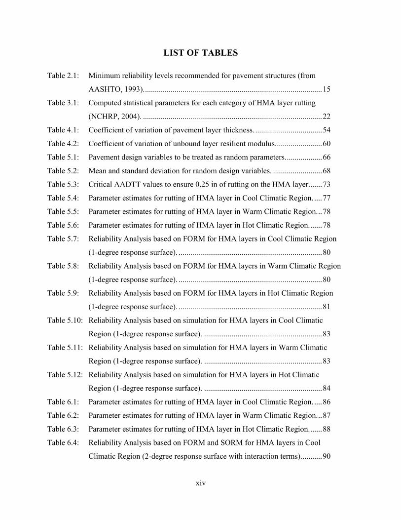
The MEPDG is “Mechanistic-Empirical” because it uses both mechanistic and empirical

principles to predict pavement performance. First, it employs a mechanistic approach by making

use of a multi-layer elastic or finite element analysis to calculate stresses and strains on the

pavement structure due to traffic loading and weather patterns forecasted for the pavement

structure that is to be designed. In a second stage, pavement responses (stresses or strains) are

used to predict (by means of empirical models) how the performance of a pavement structure

will evolve through the design period. Figure 2.1 conceptually shows the processes involved in

the MEPDG analysis procedure.

The MEPDG includes empirical models to predict rutting, top-down cracking, bottom-up

cracking, thermal cracking, and smoothness on flexible pavement structures and transverse

cracking, faulting, punchouts, crack width, load transfer efficiency, crack spacing, and

smoothness on rigid pavement structures (NCHRP, 2004; AASHTO, 2008).

Figure 2.1: Schematic of processes involved in the MEPDG (from NCHRP, 2004).

In order to perform a pavement analysis using the MEPDG, detailed information on climate,

material properties, traffic, and the pavement structure is required. These data are then used to

determine pavement response (the mechanistic component of the design process) on a bi-weekly

basis. The pavement response is finally used to estimate cumulative damage for different distress

types by means of models that have been calibrated using pavement sections that are located

11

throughout North America (the empirical component). These models are often referred to as

performance models or transfer functions.

The MEPDG can also be viewed as an iterative analysis tool since the outputs that are obtained

are different pavement distress types and roughness over time, and not layer thicknesses. Based

on AASHTO (2008), the MEPDG design process should be as follows:

1. Selection of design strategy (which can be based on other design methodologies).

2. Selection of the acceptable performance loss (failure criteria).

3. Obtaining all the input information required to run the MEPDG at the desired level.

4. Running the MEPDG and checking the reasonableness of the inputs and outputs.

5. Revise the design strategy from “Step 1” as needed.

Depending on the quality of the information available to the designer, the design can be

classified as Level 1, 2, or 3. A Level 1 design is very data intensive and requires detailed

project-specific traffic, material, and environmental information, while a Level 3 design can be

performed when the knowledge of the involved variables is more general (e.g. state or regional

default values).

2.2. FACTORS AFFECTING PAVEMENT DESIGN

The performance of the pavement structure is a function of several factors that have to be

considered regardless of the design procedure that is used. The most important parameters that

any design methodology should capture are traffic, environmental conditions, and structure and

materials. Additionally, there are other factors that have an effect on how the pavement structure

will perform in the field after it has been designed that cannot be directly accounted for in design

process, such as construction quality and preventive and routine maintenance activities.

2.2.1. Traffic

Pavement structures are designed to support a given amount of traffic throughout their services

lives. Traffic loading is a very difficult variable to characterize and forecast for the designer and

the traffic demand modeler. Furthermore, traffic loading estimates can digress considerably from

the actual values that will be observed in the field, resulting in performance noticeably different

to that which was originally predicted in the design (Hass et al., 1994).

12

Traffic loads are applied to the pavement structure by a wide variety of vehicles, ranging from

light passenger vehicles with single axles which cause virtually no structural damage to the

pavement structure, to considerably heavier trucks that carry the load on single, tandem, tridem,

or quadruple axles and can cause failure of the pavement structure due to the high stresses and

strains induced on the structure. In order to properly consider traffic in the pavement design

process several traffic related variables such as axle load distribution, axle geometry, wheel

load, tire pressure, traffic speed and traffic wandering, directional and lane traffic distributions,

traffic growth trends, and load duration and distribution have to be considered.

Because of the difficulty involved in characterizing the traffic demand, different approaches to

how traffic is accounted for in the design process have been used. In the case of the AASHTO

1993 design methodology all axles are converted to 18-kip equivalent single axle loads (ESALs)

as a method of capturing cumulative loading. The conversion to ESALs is done by means of

Axle Load Equivalency Factors (ALEFs) (AASHTO, 1993). Based on Prozzi and Hong (2007),

ESAL can be statistically described as the fourth moment of the axle load spectra.

In the case of the MEPDG, depending on the level of the design, the required information can

range from Average Annual Daily Traffic (AADT) and percentage of trucks for a Level 3 design

to axle load spectra for a Level 1 design. In order to obtain axle load spectra for the different

vehicle classes, Weight-in-Motion (WIM) stations are required. Unfortunately, WIM stations are

only located in specific locations through the United Stated, such as major Interstates Highways

or Freeways. However, this issue has been identified (Hong and Prozzi, 2006) and

recommendations for placing temporary WIM stations in under-represented climatic regions and

facility types have been made. Additionally, more general State-Level axle load spectra have

also been developed for some states such as Texas (Hong and Prozzi, 2006).

2.2.2. Environmental Conditions

Environmental conditions have an important effect on the performance of flexible and rigid

pavements, as well as on material properties. The environmental factors that have a major

13

influence in pavement performance are moisture and temperature. Some of the effects of

moisture and temperature are the following (NCHRP, 2004):

• Change in modulus of layers containing asphalt binder due to the visco-elastic nature

of the material.

• Increase in modulus of the unbound and granular materials under freezing

temperatures, due to the formation of ice. However, under thawing conditions, water

is trapped below the surface causing significant hydrostatic pressure under loading, as

well as a considerable decrease in the strength of the unbound and granular materials.

• Temperature and moisture gradients can have a direct effect on the stresses and

strains of the upper layers.

• An increase in moisture content decreases the modulus of unbound materials,

increases the stresses in the pavement structure due to hydrostatic pressure or suction,

and can affect the bonding or cementing properties of the bound materials.

Additionally, solar radiation has a hardening effect (photo-oxidation) on asphalt pavement

surfaces causing the volatilization of the lighter components of the asphalt binder (Read and

Whiteoak, 2003). This can be associated with an increase in pavement stiffness and loss of

flexibility.

2.2.3. Structure and Materials

Regardless of the type of pavement to be designed, ultimately it is the materials used in the

different layers that determine the performance of the pavement structure. Therefore it is

extremely important to identify material properties that accurately characterize the materials in

question (NCHRP, 2004).

Design material inputs can range from extremely detailed material properties that require

sophisticated laboratory testing and equipment to very simple and empirical material properties.

Some of the material requirements of current ME design guides are summarized in the following

paragraphs.

14

In the case of hot-mix asphalt (HMA), it is important to have fundamental material properties

such as dynamic modulus (E*) master curves (to cover all temperature and loading frequency

combinations of interest) and Poisson’s ratio. Additionally, other indicators of strength such as

indirect tensile strength (ITS) can be used. Furthermore, viscosity of the asphalt binder and

volumetric properties of the asphalt mix have an effect on performance.

For Portland cement concrete (PCC) materials, variables such as elastic modulus (E), Poisson’s

ratio, unit weight, and thermal expansion coefficients are of interest. Additionally, as with most

PCC structures, tensile strength, compressive strength, modulus of rupture, water-to-cement

ratio, cement type and content, among other variables are of interest and have a significant effect

on the construction and performance of the PCC layers.

In the case of unbound base and subbase layers and subgrade materials, designers are typically

interested in resilient modulus (MR) adjusted for seasonal variations, Poisson’s ratio, unit weight,

and coefficient of lateral pressure. Additional parameters that should be included in the design

process are plasticity index (PI), material gradation, specific gravity, and optimum moisture

content. For chemically stabilized materials, elastic modulus (E) is also required.

Finally, if the pavement structure is close to the bedrock, its elastic modulus (E), Poisson’s ratio,

and unit weight need to be accounted for, as well as the depth to the location of the bedrock.

2.2.4. Interaction between design variables

It is important to highlight that the effects of the previous design variables are, in general, not

independent from one another and an adequate design model should try to capture these

interactions as well as possible. Critical conditions can occur when some of the previous

variables combine in specific settings, i.e., an increase in traffic loading under very warm

temperatures on a flexible pavement structure can lead to considerable rutting and shoving

(Huang, 2003), or a decrease in the lighter or more volatile components in the asphalt binder due

to several factors (aging) can facilitate the cracking of the pavement surface due to the increase

in stiffness.

15

2.3. RELIABILITY IN CURRENT PAVEMENT DESIGN METHODOLOGIES

Before introducing the different reliability concepts from previous and current design

methodologies, it is important to understand what levels of reliability pavement structures are

typically designed for. As with any design, higher reliability levels are required for high

importance structures, and lower levels can be selected when designing less critical structures. In

the case of pavements, higher levels of reliability are typically selected for higher volume or

functionality roads. The opposite is the case of local or low volume roads. Table 2.1 shows what

are the minimum reliability levels recommended by the AASHTO (1993). Note that the levels of

reliability that are used in the design of pavement structures are very different than those used in

civil structures which tend to have expected probabilities of failure in the order of 10-4 or lower.

Table 2.1: Minimum reliability levels recommended for pavement structures (from AASHTO,

1993).

Functional

Classification

Minimum Recommended

Level of Reliability (%)

Urban Rural

Interstate and Other Freeways 85 80

Principal Arterials 80 75

Collectors 80 75

Local 50 50

In the case of the 1993 AASHTO Guide, the empirical design equations, e.g. [2.1], include a

term that accounts for uncertainty in the design process, also known as a “safety factor”: ZR S0.

This is a simple approach to accounting for reliability since it consists of using the inherent

variability associated with the model to provide confidence intervals that are then used to define

tolerances for pre-selected reliability levels. There are several limitations to this approach,

among which are the assumption that the data are distributed normally but, more importantly; it

is not possible to directly account for variability in material properties, climatic and geographical

differences, traffic, etc., separately. Furthermore, the empirical model was developed without

accounting for possible correlation between the design variables (assumption of independence),

16

such as correlation between different layer thicknesses which have been demonstrated to be

related as a result of the construction process (Aguiar-Moya et al., 2009).

This type of approach to reliability might not always be appropriate since it depends on the

standard deviation of the model (which is in turn also dependent on the statistical modeling

techniques that were used in developing it). The standard deviation is mostly intended as an

indicator of the accuracy of the predictions of the model. In the recently released Mechanistic-

Empirical Pavement Design Guide (MEPDG) a similar approach to the one above has been used

(ARA, 2004). The probability of failure is calculated using a normal distribution-based

probability (with mean predicted by the distress model and standard deviation derived as a

function of the distress itself) of exceeding the pre-specified distress threshold for failure

(AASHTO, 2008). However, as with the 1993 AASHTO Guide, one can ask if such a

simplification for the consideration of reliability is robust. What happens when the variability of

the different factors considered in the design or analysis of a pavement structure are directly

considered? What is the true reliability of a given pavement structure?

Note that even though the empirical models for pavement performance in the MEPDG are shown

in closed form, they require inputs from the structural response model (mechanistic analysis) that

are estimated for bi-weekly intervals over the design life of the pavement structure. This is a

great limitation in directly attempting to perform reliability analysis using simulation methods

because the MEPDG analysis has no closed form solution and each run of the model is time-

consuming. Furthermore, running the MEPDG several hundreds or thousands of times requires

significant computational effort and resources.

More specific details on how reliability is accounted for in the AASHTO Guide and the MEPDG

are presented in the following chapter.

17

CHAPTER 3: RELIABILITY

Reliability can be defined as “the probability that a component or system will perform a required

function for a given period of time when used under stated operation conditions (Ebeling,

2005)”. Simply stated, it is the probability of non-failure for a given period of time. For the case

of pavement structures, the definition of failure needs to be clearly described and can be a

structural or a functional type of failure.

A structural failure type corresponds to modes of failure where the pavement structure has lost

its load bearing capacity (e.g. excessive cracking, moisture damage, or rutting). Functional

failure type can be associated to cases where the pavement structure is still structurally sound but

has damage that affects its normal use (e.g. excessive roughness).

Once the proper failure modes have been identified, the threshold for each one of them has to be

clearly defined (this defines the limit states). Otherwise, the subjective issue of what might be

acceptable to some might not be to others arises.

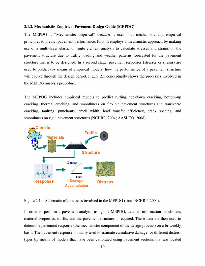
Mathematically, the definition of probability of failure ( ) might be stated as,

= ( ( ) ≤ 0) = … ( )( ) [3.1] where g (.) is the limit state function (function that separates the failure and non-failure

domains). The probability of failure corresponds to a violation of the limit state. g (.) is a

function that defines the relationship between the limit state or failure and the variables that have

been determined to have an effect on it (X). ( ) is the density function of the variables that are

used in the limit state function, ( ).

Then reliability can be expressed as = 1 − [3.2]

18

Therefore, estimation of reliability involves solving a multidimensional integral that can rarely

be solved analytically. Two different approaches to solving [3.1] have been used in the literature

(Melchers, 1999),

• Numerical approximations to solve the multidimensional integration, such as

simulation (Monte Carlo Methods).

• Transforming the probability density function ( ) in [3.1] into a multivariate

normal probability density function, and using some of the properties of the

multivariate normal probability density to approximate and R.

The two previous approaches are covered in Sections 3.4 and 3.5 of this Chapter.

3.1. RELIABILITY IN THE AASHTO GUIDE

In the AASHTO Guide for Design of Pavement Structures (1993) reliability is defined as: “…

the probability that any particular type of distress (or combination of distress manifestations)

will remain below or within the permissible level during the design life”.

The AASHTO methodology is based on an empirical model to predict the number of equivalent

single axle loads, or ESALs (Wt) before the pavement section reaches a specified terminal level

of serviceability. The model is based on design variables such as: layer thickness, roadbed

modulus (MR), drainage and climate conditions, and pavement functional factors (terminal PSI), as per [2.1] for the case of flexible pavements. Wt represents the number of ESALs the designed

pavement structure can withstand before reaching failure (the specified terminal PSI or pt).

Simultaneously, based on traffic data from traffic counts, WIM stations, or other methods, wt (predicted number of ESALs the pavement section will be subjected to) is determined.

Ultimately, Wt represents the supplied capacity, while wt represents the demand or load that will

be applied to the pavement structure.

Based on the AASHTO methodology, the reliability design factor, based on wt and Wt, is

defined as

19

= [3.2]

Additionally, under the assumption that the factors affecting the variability of Wt, and

consequently wt, follow a log-normal distribution, the logarithm of Wt is used in order to induce

normality in the probability distributions. Then it follows that, ( ) = ( ) − ( ) [3.3]

Eq. [3.3] also represents the reliability design factor, but is solely based on the predicted capacity

and traffic demand that the pavement section will be subjected to. However, in order to introduce

the variability of the actual performance the pavement section will experiment, as opposed to the

predicted one; an overall variation of δ0 is introduced and defined as, = ±[ ( ) − ( )] [3.4]

Where Nt is the actual capacity the pavement structure will provide and nt represents the actual

demand the pavement structure will have to support. The previous definition of overall variation

is used to define reliability as, = 1 − ( ≥ ) [3.5] = 1 − ( ≥ 0) [3.6]

Standardizing δ0, and defining S0 as the as the overall variation (accounts for chance variation

and traffic prediction variation), the standard normal deviate is defined as, = − = − ( ) [3.7]

And under the assumption that on average, δ0 for the population is 0, = − ( ) → ( ) = − [3.8] where ZR is used to select the different levels of reliability to be considered in the design of the

pavement structure. The reliability levels are assigned based on the relative importance of the

pavement structure.

20

The approach has the limitation that the overall variation values that are used have also been

developed for very specific conditions that might not generally apply to current pavement

technologies. This has been demonstrated by Prozzi et al. (2005) by analyzing the reliability of

AASHTO method designs by means of simulation. The researchers considered the thickness of

the different pavement layers and the weekly traffic as random variables. They found that the

AASHTO reliability level usually differs significantly from the actual reliability of the pavement

structure, in some cases by as much as 40%.

Rogness (1988) also raised the issue of reliability versus functional class in the 1993 AASHTO

Guide. The researcher suggests that there should be distinction in the consequences of failure of

different functional classes of pavement structures. Another limitation that is highlighted by

Rogness (1988) is that the AASHTO Guide does not allow for considering reliability of a staged

construction process. This means that the reliability is set to a fixed level for the entire pavement

structure, but it is impossible to assign different variability to each pavement layer individually.

To address some of the previous limitations, Kim et al. (2002) proposed using a different

procedure for estimating the reliability of pavement structures designed using the 1993

AASHTO Guide. The researchers suggested a 2-step Load and Resistance Factor Design

(LRFD) approach, similar to ones applied in the design of bridges and other concrete or metal

structures. In the first step, the performance of the pavement structure is determined and in the

second step, reliability is estimated by means of analytical approximations.

Alternatively, Kulkarni (1994) suggested replacing the term in the AASHTO design

equations by a safety margin that is a function of previously assumed distributions of the Wt and wt. 3.2. RELIABILITY IN THE MEPDG

Reliability in the MEPDG is defined as that probability that a given distress type (distressi) does

not exceed the critical limit for that type of distress over the service life of the pavement

structure (NCHRP, 2004). Mathematically it can be expressed as, = Pr( of design project < critical over design life) [3.9]

21

In order to calculate [3.9] it is assumed that distressi follows a normal distribution. The

normality assumption can be to used estimate the critical distressi for any reliability level R as = + [3.10] where ZR is the standard normal deviate for a given level of R, is the average predicted distressi from the MEPDG analysis (MEPDG output for distressi at any given time t), and is the standard error associated with distressi. is expected to capture the variability in the prediction due to material variability,

traffic and environmental variability, and modeling errors. The functional shape of is

different for the different distress types, but in general it is defined as a function of the predicted

distress by means of the MEPDG analysis, or, = ( ) [3.11]

The ′ were estimated based on the same data that were used to fit the MEPDG

models as follows. The first step in the estimation of the standard error consisted of estimating distressi for all the different pavement sections that were used in estimating the MEPDG

empirical performance models. Then, the predicted distressi were categorized based on the

severity of the distress. For example, in the case of rutting in the HMA layer the predictions

where categorized in the following ranges: 0.0 – 0.1 in, 0.1 – 0.2 in, …, 0.5 in and above.

The second step in estimating the model standard error involved computing the following

statistics for each of the categories defined in the previous step: expected (predicted) distressi, existing distressi (average), and the standard error for the estimate of distressi. The predicted

and observed averages for each category were then compared (to “verify” the quality of the

predictions). In the third step, an empirical relationship between the expected (predicted) distressi and the standard error for the estimate of distressi was developed by means of

regression.

Continuing with the previous example of rutting in the HMA layer, the statistics estimated as

part of the second step in the estimation of the standard error are summarized in Table 3.1.

22

Table 3.1: Computed statistical parameters for each category of HMA layer rutting (NCHRP,

2004).

Category

(in)

Expected

(Predicted)

Rutting (in)

Average

Measured

Rutting (in)

Standard Error

for Expected

Rutting (in)

Sample

Size

0.0 – 0.1 0.05 0.06 0.03 219

0.1 – 0.2 0.14 0.15 0.06 153

0.2 – 0.3 0.24 0.12 0.09 61

0.3 – 0.4 0.35 0.30 0.13 20

0.4 – 0.5 0.43 0.32 0.15 11

0.5 or more 0.74 0.67 0.09 6

Finally, based on the previous statistics, the following model was fit as part of the final step in

estimating the standard error for the HMA rutting performance model in the MEPDG, = 0.1587 . [3.12]

As with [3.12], standard error models with slightly different functional forms were fit for all the

distress models included in the MEPDG. Finally, based on the standard error estimated by means

of models such as [3.12], the critical distressi for any reliability level R can be estimated, as per [3.10].

Unfortunately, the previously described method of estimating the standard error for a given

prediction is biased because:

1) the model predictions are being grouped into small ranges, therefore decreasing the

“true” variability of the distressi model,

2) the standard error model is being estimated in several stages, thereby reducing the

efficiency of the model and introducing additional error since the prediction is based on

previous estimates of distressi as opposed to actual observed performance, and

3) most of the data points used in the estimation are not properly distributed along the

entire range of possible observed distress types, but correspond to specific levels of the

23

given distress for which the standard error model is being estimated (e.g. in the case of

rutting on the HMA layers, most of the observations used in predicting both the

performance model and the corresponding standard error model are in the range of 0.0 –

0.2 in, but almost no observations have rutting greater than 0.5 in; Table 3.1). This

introduces upward or downward bias in the standard error estimates.

The author believes that a more efficient method to estimate the reliability of a pavement design

using the MEPDG would be to directly use the regression standard error ( ) that is obtained

when the parameters for are estimated, while also accounting for heterogeneity. is a

more efficient estimator of the standard deviation of the distribution of the unobserved factors

affecting distressi, ui (Wooldridge, 2002). Additionally, using reduces the need of

introducing additional error to the standard error estimate by calculating it in a separate step.

Nonetheless, regardless of whether or is used in the reliability analysis of a given

pavement design, the considerable drawback of both approaches is that they do not allow for the

possibility of accounting for the true variability of distressi due to non-homogeneity of material

properties, loading and environmental conditions, as well as structural variability due to the

construction process.

The previous is not an issue in the estimation of since it is basically an average

measure of distressi given deterministic values of the different factors that have been identified

to have an effect of in. However, the variables that are used in estimating distressi are stochastic

in the sense that their values are not fixed but actually follow specific distributions, and changes

in each of this variables have an effect on the performance of the pavement structure and,

therefore, on the reliability of the pavement structure.

Given the previous limitations in the estimation of reliability of the MEPDG (an equivalently the

1993 AASHTO Design Guide), the focus of the current research is to propose a robust

methodology that can be used to properly estimate the reliability of a pavement structure, based

on the ME performance predictions of the MEPDG.

24

3.3. UNCERTAINTIES IN THE ESTIMATION OF RELIABILITY

As with the estimation of pavement performance, which in this case is directly linked to the

reliability of the pavement structure, there are many factors that introduce variability to the

estimation of reliability (De Bièvre, 1996).

Due to the uncertainty associated with the reliability estimation process, the results that are

obtained are something that concerns most civil engineers. Several types of uncertainty directly

affect the models and estimates that are developed to predict performance and reliability of

structures. This is especially true in the case of pavement engineering where we often evaluate

the properties of rather heterogeneous mixes of materials under very variable sets of conditions

and where, in many cases, the testing procedures and equipment vary greatly from one region to

the next.

Among the factors that introduce uncertainty into the estimation of reliability are: uncertainty in

measurement, uncertainty in material properties, uncertainty in structural, and environmental

conditions, uncertainty in the modeling process, uncertainty in performance and parameter

estimation (statistical, econometric uncertainty), and human error (Melchers, 1999).

Some of these types of uncertainty can be minimized by following standardized testing

procedures with properly calibrated and maintained testing equipment (measuring uncertainty) or

by properly training and certifying equipment operators and surveyors (human error). Other

types of variability can not necessarily be controlled (environmental uncertainty) but need to be

properly accounted for. Similarly, material and structural uncertainty can be reduced to some

degree by following a proper quality control and quality assurance (QC/QA) process.

Regardless of the type of uncertainty, a proper reliability analysis needs to capture the variability

of the system so that a proper estimate of the true probability of failure of a given pavement

structure can be obtained.

The importance of accounting for uncertainty has been highlighted by Ayres and Witczak (1998)

with the AYMA system. AYMA is a pavement performance program that incorporates some of

25

the most widely accepted fatigue cracking, permanent deformation, and low temperature

cracking models with the distinction that the user can not only input mean values for the input

parameters, but also a measure of variation. Although the program is limited to the assumption

that all variables are normally distributed, the authors have shown that the performance models

are highly sensitive to the variation in the input parameters.

Brown (1994) also highlights the value of estimating and correctly accounting for the variability

in all the inputs associated with a particular design methodology. Knowledge on the uncertainties

associated with the different variables gives the pavement designer the opportunity to examine

what is the overall contribution of the each one of them to the overall system variability. This, in

turns, permits more effort to be assigned to the factors that have a higher or more detrimental

effect on the performance of the pavement structure.

As a final comment, the risks of using the results of a deterministic pavement analysis or design

procedure (one based only on the mean values of the input parameters) have to be noted. When

performing a deterministic design, the outputs of the models correspond only to the mean

predicted values. However, in reality none of the inputs that are required by a given deterioration

model are fixed but have been estimated from field or laboratory observations and have a

distribution associated with them. In some cases, the variability might be considerable.

Furthermore, it is possible that the variations on the input parameters can greatly decrease the

expected performance of the pavement structure being designed.

3.4. RELIABILITY BY MEANS OF SIMULATION TECHNIQUES

Simulation techniques consist of randomly sampling the variables that affect the performance of

the pavement structure a large number of times and analyzing the outcomes or results (Melchers,

1999). Based on these results, probabilistic response properties can be estimated. The most

widely applicable simulation technique is crude Monte Carlo Simulation.

An important concern with crude Monte Carlo simulation is that solving a large number of

deterministic instances of the performance or limit failure state function is required.

Additionally, it has been shown that generally, in order to obtain reliable results the number of

26

iterations needs to be in the order of thousands (Osnes, 1997). Therefore, in order to ensure the

accuracy of crude Monde Carlo Simulation, several variance reduction simulation techniques can

be used. Some of the variance reduction techniques that are more commonly used are:

Importance Sampling, Antithetic Variates, Latin Hypercube, and Systematic Sampling. The

variance reduction simulation techniques are expected to converge faster to the “true” probability

of failure as compared to the crude Monte Carlo simulation procedure.

For completeness, a brief description of the previously mentioned simulation techniques follows

(Manuel, 2008; Osnes, 1997),

• Crude Monte Carlo: consists of generating N random data points for each random

variable based on the distribution of the random variables included in the analysis,

estimating the value of the failure function for each vector of random variables, and

counting the number of failures that are observed within the N samples. The probability

of failure is given by, = [1( ( ) ≤ 0)] ≅ ∑ 1( ( ) ≤ 0) [3.13] Where 1( ( ) ≤ 0) is an indicator function that is equal to 1 if ( ) ≤ 0 or 0

otherwise. Finally, the simulation is repeated several times to determine the variability of

the estimate.

• Importance Sampling: the sampling of random variables is done based on an importance

sampling function ℎ ( ) as opposed to the initially assumed distribution of the random

variables ( ). This is accounted for by factoring the observed failures by the ratio of

density functions, or, = 1( ( ) ≤ 0) ( )ℎ ( ) [3.14] The importance sampling function should be selected by shifting the means of the

distributions slightly towards the limit state to ensure that failures are observed.

• Antithetic Variates: this method is based on combining two unbiased estimates of the

probability of failure and hence reducing the variance of the estimation by four. This is

achieved by generating N independent uniform [0,1] random variables, ′, and defining = 1 − ′. Then, the desired correlated random variables are estimated as =

27

( ′) and = ( ′′). The failure function is then evaluated at and , and the

respective probabilities of failure are = [1( ( ′) ≤ 0)] and = [1( ( ′′) ≤0)]. Finally, the antithetic estimate of the probability of failure is, = 12 + [3.15] • Latin Hypercube: instead of randomly drawing from the distribution of each random

variable, the probability space is divided into N strata, and a sample is randomly drawn

from each strata for each random variable. Once the random variables have been

sampled, the probability of failure is estimated as, = [1( ( ) ≤ 0)] [3.16] • Systematic Sampling: very similar to the Latin Hypercube method of variance reduction,

but in place of drawing a random sample from each strata for the random variables, the

mean value of each strata is selected as sample data point. The probability of failure is

calculated as in [3.16].

Additionally, combinations of the previous variance reduction techniques can also be applied

(Osnes, 1997).

Alsherri and George (1988) used crude Monte Carlo simulation to solve the AASHTO design

equations under the assumption that all the input variables are probabilistic, independent and

normally distributed. Crude Monte Carlo simulation has also been used by Prozzi et al. (2005) to

evaluate the reliability of pavement designs using the AASHTO Design Guide under various

traffic levels. It was found that the AASHTO design tend to be overly conservative. The

simulation analysis was also useful for identifying that the surface asphalt mix layer thickness

and the performance model error have the highest relative influence on the reliability of the

pavement structure. The researchers then proceed to highlight the importance of including the

model error as part of the variability on the overall performance of the structure.

A simple reliability analysis based on Monte Carlo simulation with variance reduction was also

initially suggested by Timm et al. (2000) and implemented by Chadbourn (2002) for the

mechanistic-empirical (ME) pavement design procedure MnPave (MnDOT Flexible Pavement

Design: Mechanistic-Empirical Method). The reliability analysis was used on the fatigue

28

cracking and rutting transfer functions where the required inputs for the program are thickness

(μ, CV)1, elastic modulus (E), and Poisson’s ration (ν). Because of the computing and time

constraints involved in using simulation with the ME procedure, the researcher proposed

estimating the reliability of a comprehensive set of conditions and then fitting a “reliability

regression function” based only on predicted damage from the MnPave transfer functions

(reliability as a function of damage) to allow for a quick estimation of reliability in the design

process.

3.5. RELIABILITY BY MEANS OF SECOND MOMENT TECHNIQUES

The second moment techniques consist of using the first two moments (mean and standard

deviation) of each variable (and correlation coefficients when necessary) involved in the

probability failure estimation to represent them and to simplify the estimation of the integral in [3.1]. 3.5.1. First Order Reliability Method (FORM)

In the First Order Reliability Method (FORM), the limit state function ( ) is linearized by

means of a Taylor series expansion and the distance to the failure surface from the origin in the

space of the random variables is minimized (β). The reliability index β represents the minimum

distance from the origin of the design random variable space to the failure surface. β is also

sometimes known as the reliability index or the safety index, and indicates the boundary of the

failure region (Melchers, 1999). Therefore, β can be used as a measure of the safety or reliability

of a structure: greater β represents a lower probability of failure .

FORM is based on the assumption that a probability preserving transformation = ( ) exists

such that u is a vector of independent standard normal variables (Rackwitz, 2001). Then, under

the previous assumption,

= … ( )( ) = … ( )( ) [3.17]

1 Where μ is the mean value, σ is the standard deviation, and CV is the coefficient of variation (σ /μ).

29

The transformation can be performed exactly in the case where X consist of non-correlated

random variables by means of Cholesky decomposition. In the case of correlated random

variables, with the exception on a normal log-normal transformation which can be performed

exactly, approximate transformations by means of the Rosenblatt-transformation or the Nataf-

transformation are required.

Under the assumption that the limit state function is differentiable and because of the rotational

symmetry of the standard normal density, it results that the reliability index β can be directly

used to compute the probability of failure as = Φ(− ) in the case that the design random

variables are normally distributed and the failure state function is linear (Lee et al., 2002). For a

nonlinear limit state functions, the solution is approximate, i.e., ≈ Φ(− ). Φ(∙) corresponds

to the standard normal integral or standard normal cumulative density function.

The design point ∗ = ( ∗) corresponds to the point along the failure surface ( ) where the

distance to the origin of the design parameters is minimum. Then under FORM, = ‖ ∗‖ and ∗ can be estimated by, ∗ = ‖ ‖ ∀ : ( ) ≤ 0 [3.18]

Geometrically, the concept of the reliability index (minimum distance from origin to design point

in a standard normal space) is described in Figure 3.1. Note that U corresponds to variables in a

standard normal space resulting from a transformation/mapping from the original space of the

physical random variables X

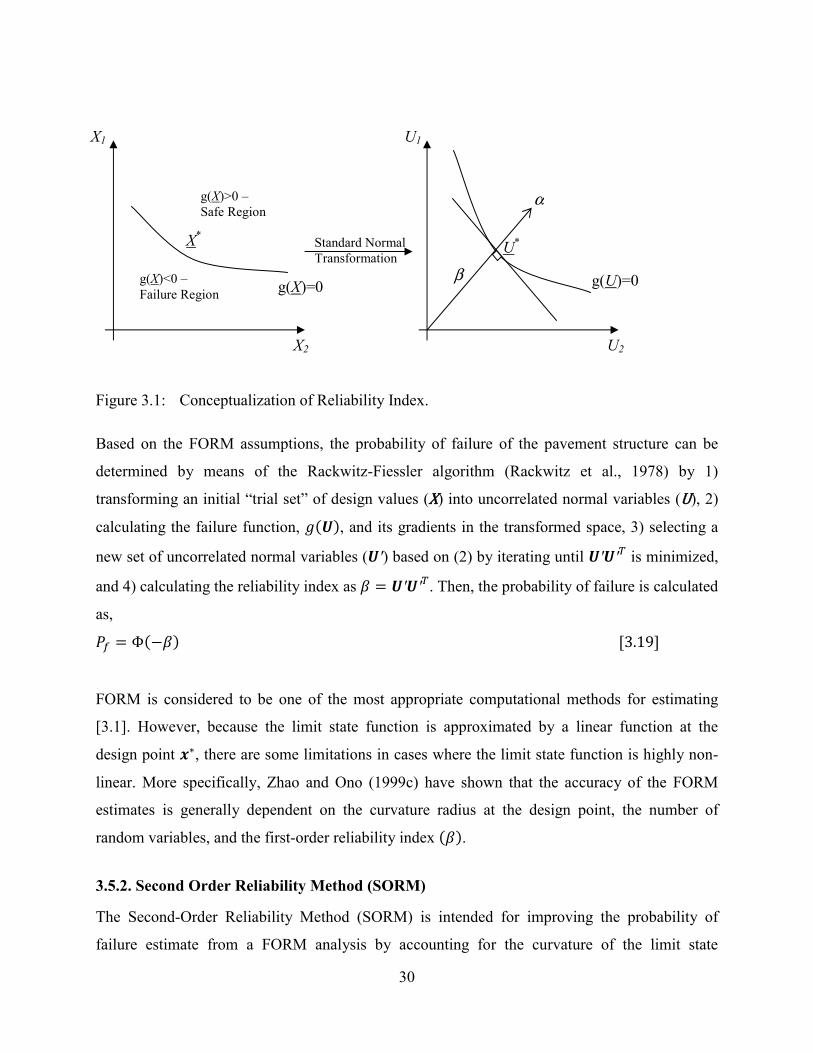
30

Figure 3.1: Conceptualization of Reliability Index.

Based on the FORM assumptions, the probability of failure of the pavement structure can be

determined by means of the Rackwitz-Fiessler algorithm (Rackwitz et al., 1978) by 1)

transforming an initial “trial set” of design values (X) into uncorrelated normal variables (U), 2)

calculating the failure function, ( ), and its gradients in the transformed space, 3) selecting a

new set of uncorrelated normal variables ( ′) based on (2) by iterating until ′ ′ is minimized,

and 4) calculating the reliability index as = ′ ′ . Then, the probability of failure is calculated

as, = Φ(− ) [3.19]

FORM is considered to be one of the most appropriate computational methods for estimating

[3.1]. However, because the limit state function is approximated by a linear function at the

design point ∗, there are some limitations in cases where the limit state function is highly non-

linear. More specifically, Zhao and Ono (1999c) have shown that the accuracy of the FORM

estimates is generally dependent on the curvature radius at the design point, the number of

random variables, and the first-order reliability index ( ).

3.5.2. Second Order Reliability Method (SORM)

The Second-Order Reliability Method (SORM) is intended for improving the probability of

failure estimate from a FORM analysis by accounting for the curvature of the limit state

g(X)=0

X1

X2

g(X)>0 – Safe Region

g(X)<0 – Failure Region

X*

g(U)=0

U1

U2

β U*Standard Normal

Transformation

α

31

function. This is done by including additional information of the curvature of the limit state

function by means of second-order derivatives of the limit state function with respect to each

random variable. The correction can be approximated as follows (Breitung, 1984),

≈ (− ) (1 + ) [3.20] where corresponds to the principal curvatures of the limit state function at the minimum

distance point identified by a FORM analysis. This is achieved by rotating the uncorrelated

random normal vector from the FORM analysis such that one of the variables aligns with

the direction cosine vector = −∇ ( ∗)/|∇ ( ∗)| that points from the design point, ∗, to the

origin in U space. The direction cosines of the remaining ( − 1) variables in the rotated

space can be obtained by Gram-Schmidt orthogonalization resulting in an matrix. Finally, the

SORM procedure requires the estimation of an matrix which corresponds to the rotation of the

matrix of second derivatives of the limit state function (Hessian) as, = | ( )| [3.21] The curvature corresponds to the j-th eigenvalue of the (i–1) x (i–1) submatrix of .

It has been demonstrated that asymptotically SORM cannot be improved (Breitung, 1994). In the

non-asymptotic case higher-order corrections can be used, however, very few results have been

developed (Yao and Ono, 1999a; Yao and Ono, 1999b; Yao et al., 2002).

Cizelj et al. (1994) have also shown that the performance of numerical techniques such as FORM

and SORM is very good (even more so for the case of SORM) when comparing the relative

errors of FORM and SORM to different types of Monte Carlo simulations (based on different

variance reduction techniques: IS – importance sampling, AS – adaptive sampling, and ES –

efficient sampling). Figure 3.2 shows the comparison of the different reliability approaches used

by Cizelj et al. (1994) when evaluating cracking on steam generator tubing (PL or plugging limit

represents the length of crack when tubes are taken out of service).

32

Figure 3.2: Comparison of relative error from reliability estimates based on FORM and SORM

to different Monte Carlo simulation estimates for cracking on steam generator

tubing (from Cizelj et al., 1994).

Equivalent results were obtained by Zao and Ono (1998) when comparing the reliability of

ductile frame structures by means of FORM and SORM.

As for pavement structures, the second moment reliability index (which can be estimated by

FORM) has been used to evaluate the reliability of pavement structures designed using the 1993

AASHTO Guide by Zhang and Damnjanović (2006). The authors found errors less than 1%

when comparing the second moment reliability estimates to those obtained by crude Monte Carlo

(Figure 3.3).

33

Figure 3.3: Pavement failure probabilities by Second Moment (and higher order moments) and

crude Monte Carlo simulation (from Zhang and Damnjanović, 2006).

3.6. RESPONSE SURFACE APPROACH TO RELIABILITY

Without prior knowledge of the true reliability (as would be estimated by using the MEPDG) of

a pavement structure, it is difficult to determine the number of simulations that would be

required to estimate the reliability of the pavement structure with any specified level of

confidence. Therefore, in order to ensure that an accurate estimate of the true reliability of the

pavement section has been found, simulation with a large number of repetitions is initially

required. This is a limitation because of the time that is required to run a single instance of the

MEPDG. Additionally, because there is no closed-form solution to the analysis performed by the

MEPDG, no exact probability of failure can be computed. Furthermore, because access to the

source code of the MEPDG is restricted, it is difficult to integrate the MEPDG analysis into a

simulation or second moment reliability approach. It also has to be noted that the mechanistic

component of the MEPDG consists of a finite element (FE) or a multilayer linear elastic analysis

and can require considerable amounts of computing power when many instances of the MEPDG

have to be run.

34

For these reasons, a response surface approach to defining the limit state function is proposed in

this study. A response surface is an approximation to the true limit state function or failure

function that can be found by fitting a model, usually of polynomial form, to serve as a

representation of the true limit state function. Response surfaces are generally fit within a small

range of variation of the design variables to ensure that the predictions estimated by the response

surface closely match those that would be obtained by running the MEPDG under a given set of

conditions.

Although the use of response surfaces for estimating reliability is not common in pavement or

transportation engineering, they have been widely used in other areas of civil engineering,

mainly in structural and geotechnical applications. Some of the applications are summarized in

the following paragraphs.

Su et al. (2009) have used a response surface approach in combination with crude Monte Carlo

simulation to evaluate the reliability (due to aerostatic response and aerostatic stability) of long-

span bridges, while considering the geometric parameters, the material parameters, and the

aerostatic coefficients as random variables. The response surface approach was used because of

the finite element analysis that is used in long-span bridge analysis would require considerable

computing power that was not readily available.

Mollon et al. (2009) used response surfaces to evaluate the reliability of circular tunnels in

homogeneous soils. Response surfaces were used because the analysis of tunnels involves

numerical simulations that have no closed form solutions. Therefore, the authors used response

surfaces to estimate the reliability index and design point by approximating the performance

function by a quadratic explicit function of random variables. Gui et al. (2008) applied a similar

approach to estimate the reliability of high rock slopes in hydropower projects while considering

several slip surfaces.

Similarly, Xu and Low (2006) have used response surfaces to fit the stability curve of slopes and

embankments because of the increase in use of the finite element method to perform

deterministic stability analysis. The authors use the response surface along with FORM to

35

estimate the reliability index of slopes and embankments. An important finding from this study is

that, in cases when the response surface is close to being planar, the reliability index can be

predicted quite accurately.

In a similar approach, Chan and Low (2009) used the response surface method to evaluate the

reliability of laterally loaded piles under nonlinear soil and pile behavior. The researchers

evaluated the reliability index from FORM based on two different failure modes, while

considering non-normal, correlated variables. The researchers also compared the probability of

failure from FORM to the one obtained from crude Monte Carlo simulation to find errors of the

magnitude of less than 10%.

Lee and Haldar (2003) and Yao and Wen (1996) have also observed the efficiency of the

probability of failure estimates (as compared to direct simulation results) when analyzing the

reliability of frame and shear wall structural systems and stationary single-degree-of-freedom

(SDOF) systems subjected to white noise excitation.

Figure 3.4: Comparison of direct simulation to simulation based on response surfaces for

SDOF systems (from Yao and Wen, 1996).

Similarly, Wong (1985) showed that the statistics obtained from analyzing reliability of soil

slopes using a response surface approach varied between 1% to 9%, as compared to the statistics

obtained from direct finite element simulation.

36

Figure 3.5: Comparison of direct simulation (FE) to simulation based on response surfaces (RS)

for soil slopes (from Wong, 1985).

Babu and Srivastava (2010a; 2010b) also used response surfaces along with FORM analysis to

evaluate the reliability index of buried flexible pipelines and dams. The authors used the

response surface approach to establish a relationship between random input variables and the

response of the aforementioned structures. It can be noted that the authors also included an

uncertainty term (ε) in the response surfaces to capture uncertainty that is unaccounted for. The

uncertainty term, ε, is treated as regression error with its associated mean and standard error ( , ).

Rajashekhar and Ellingwood (1995) also used response surfaces to approximate the reliability of

reinforced-concrete cylindrical shells. The authors recommended selecting the points to be used

for fitting the response surface based on an interpolation scheme as follows, = + ( − ) ( )[ ( ) − ( )] [3.22]

Where ( , ) corresponds to the previously identified design points for the random variables

involved in the reliability determination based on [3.22], and is the mean value ( ) of the

37

random variables used in the analysis. The process is iterated while measuring the distance

between ( , ), ℎ = ( − ) and repeated until ℎ is close to zero or is zero.

Huh and Haldar (2001) analyzed the stochastic seismic risk of nonlinear structures using

response surfaces. The researchers highlight that the degree of the polynomial to be used

depends on the nonlinearity expected on the structural response. Based on the current literature

review, most of the previous researches have used one or two-degree polynomials that might

include cross terms as follows,

( ) = + + + [3.23]

38

39

CHAPTER 4: VARIABILITY IN PAVEMENT DESIGN

As has been pointed out in previous chapters, in order to assess the reliability of a pavement

structure, it is essential to have prior knowledge on the variability of the factors affecting the

performance and, therefore, the failure of the pavement structure in question.

Up to this point, several design methods have been introduced and how reliability is currently

accounted for in each one of them has been presented. However, the objective of this research is

to present a methodology to properly estimate reliability of a pavement structure, by means of

the MEPDG (Level 3), using several simulation and second moment techniques. Furthermore, as

the case study for demonstrating the application of the various methodologies, the current

analysis focuses on the reliability of a pavement structure as measured by rutting of the HMA

layers.

The selection of Level 3 is due to the assumption that the variability in the input requirements for

a Level 3 design should be higher, than that of the Level 1 input variables. Furthermore, the

analysis is based on Level 3 input variables under the assumption that the designer will have

easier access to them, as opposed to Level 1 input which require sophisticated material

laboratory testing and traffic field observations.

The Level 3 input variables that are required for the analysis of pavement structure using the

MEPDG are the following:

1. General Information:

1.1. Design life (years)

1.2. Base and subbase construction date

1.3. Pavement construction date

1.4. Date open to traffic.

2. Traffic:

2.1. Two way average annual daily truck traffic (AADTT)

2.2. Number of lanes in design direction

2.3. Percent of trucks in design direction, percent of trucks in design lane

40

2.4. Operating speed

2.5. Monthly traffic adjustment factors

2.6. Vehicle class distribution

2.7. Hourly truck distribution

2.8. Traffic growth

2.9. Axle load distribution

2.10. Traffic wander

2.11. Axle configurations, truck wheelbase, number of axles per truck

3. Climate:

3.1. Ground water table location

3.2. Climatic forecasts based on weather stations

4. Structure:

4.1. HMA Layers:

4.1.1. Gradation (retained 3/4, 3/8, No. 4, passing No. 200 )

4.1.2. Asphalt binder grade

4.1.3. Volumetric properties (binder content, air voids, density)

4.1.4. Poisson’s ratio

4.1.5. Thickness

4.2. Granular/Soil Layers:

4.2.1. Poisson’s ratio

4.2.2. Coefficient of lateral pressure

4.2.3. Modulus

4.2.4. Gradation (all available sieves)

4.2.5. Plasticity Index (PI), Liquid Limit (LL)

4.2.6. Thickness

Treating all the variables included in a MEPDG (Level 3) analysis as random would be

unfeasible because of computational and time constraints. For this reason, a reduced set of

variables that have been demonstrated consistently in the literature (Aguiar-Moya and Prozzi,

2011) to have the greatest impact on pavement performance, and in this case on rutting of the

HMA layers, has been defined.

41

The variables that were used in characterizing the reliability of a given pavement structure are

the following: climatic region, Truck Traffic Classification (TTC), Average Annual Daily Truck

Traffic (AADTT), thickness of the HMA layer, asphalt binder content, air void content,

thickness of the base, modulus of the base, and modulus of the subgrade.

The previous variables were chosen because of the effect that they have on performance

predictions by the MEPDG. In order to demonstrate this, a sensitivity analysis to rutting was

conducted on each one of these variables individually, while holding the remaining variables

fixed. The effect on roughness was also observed since roughness is related to rutting.

Additionally, it was important to assess the sensitivity of the previous variables on other distress

types. The results are shown on Figures 4.1 thru 4.6.

It can be observed from the figures that rutting on the HMA layer is highly sensitive to HMA

layer thickness, asphalt binder content, and air void content. Furthermore, rutting on the HMA

layer is also sensitive to changes in the base thickness and base modulus (although to a lesser

degree). Base and subgrade modulus also have an important effect on total rutting of the

pavement structure. Finally, note that the sensitivity of the evaluated variables is based assuming

independence between the different variables. However, in the following sections of this chapter

it will be clearly established that this is not the case.

For the case of roughness, individual changes in all the variables have an effect on it. However, it

can be noted that the variables that produce the biggest effect on roughness are the volumetric

properties of the HMA mix: asphalt binder content and air void content.

Figure 4.1: Effect of HMA layer thi

Figure 4.2: Effect of base thickness

42

ickness on rutting and roughness according to the

on rutting and roughness according to the MEPD

MEPDG.

G.

Figure 4.3: Effect of binder content

Figure 4.4: Effect of air voids on ru

43

on rutting and roughness according to the MEPD

utting and roughness according to the MEPDG.

G.

Figure 4.5: Effect of base modulus o

Figure 4.6: Effect of subgrade modu

44

on rutting and roughness according to the MEPDG

ulus on rutting and roughness according to the ME

G.

EPDG.

45

Variability in the environmental conditions is not considered, since the analysis is for a given

pavement structure at a given location. Additionally, traffic design variables are to be considered

deterministic. This is the case for variables like: axle configurations, truck wheelbase, and

number of axles per truck that have been set by truck manufacturers. Additionally, variables such

as monthly adjustment factors and hourly truck distribution are going to be assumed fixed since

there is few available data to accurately determine them and, these factors are specific to any

given segment of road.

For the previously selected variables to be considered random, information on their distributions

such as distribution type and typical standard deviations and coefficients of variations are

required. Unfortunately, research on the variability of the factors affecting the performance of a

pavement structure has been very limited and it is outdated (Darter, 1973). Therefore, the

variability of the selected variables will be determined by means of the Long Term Pavement

Performance (LTPP) Database.

4.1. THE LONG TERM PAVEMENT PERFORMANCE (LTPP) DATABASE

The Long Term Pavement Performance (LTPP) Program was started as part of the Strategic

Highway Research Program (SHRP) in 1987. The program management was transferred to the

Federal Highway Administration (FHWA) in 1992. As of data release 24.0 (2010), the LTPP

database houses over 2,500 pavement test section on in-service highways in over 900 locations

through the United States and Canada (Figure 4.7).

46

Figure 4.7: Location of LTPP GPS and SPS pavement sections (from http://www.ltpp-

products.com).

The data included in the LTPP database include inventory information, material testing,

pavement performance monitoring, climatic, traffic, maintenance, rehabilitation, and specific

seasonal testing results (Elkins et al., 2006).

A total of 791 LTPP test sections are in the General Pavement Studies (GPS) category. The GPS

sections correspond to pavement sections that were already in service when the LTPP project

began. Each test section is at a different location. Of these sections, 703 are active and 88 have

been taken out of study. When a GPS test section is taken out of study, data are no longer

collected for that section.

1,714 other test sections are in the Specific Pavement Studies (SPS) category. The SPS sections

were constructed after LTPP began, and were constructed in order to monitor the effect of

specific variables or factors in the performance of pavement structures. At each SPS location,

there is more than one pavement test section, depending on the factorial design defined as part of

47

each SPS experiment. These test sections are grouped by projects at 229 different locations. Of

the 1,714 sections, 1,508 are active and 206 have been taken out of study.

Because of the size of the LTPP database, it was selected as an appropriate source for estimating

the in-field variability of the pavement design variables that were analyzed as part of this study.

The specific sections that were chosen to characterize the variability of each variable were

selected based on the availability of the data for given GPS or SPS sections.

4.2. GOODNESS-OF-FIT TESTS FOR VARIABLE DISTRIBUTIONS

Many goodness-of-fit tests have been developed and are commonly used when characterizing the

distribution of a given variable. Some are general in the sense that they can test how well the

data fit any distribution given that the expected probabilities of the distribution can be computed.

Such is the case of the (chi-squared) goodness-of-fit test where the expected frequencies (Ei) of pre-defined data point ranges (k classes) are compared to the number of observations (Oi) in

that range (i class),

= ( − ) [4.1]

Other commonly used general goodness-of-fit tests include the Kolmogorov-Smirnov test, which

is more robust than the goodness-of-fit test in that it does not require the data to be grouped.

However, the Kolmogorov-Smirnov test has the limitation that it is only sensitive near the center

of the distribution. For this reason, the Anderson-Darling test is generally preferred for small

samples (25 observations or less) because it assigns higher weight to the tails of the distribution.

For larger samples (more than 25 observations), the minimal deviation from the expected

distribution rejects the hypothesis that the data come from a specified distribution (Anderson and

Darling, 1952).

The previous tests are applicable for testing goodness-of-fit to any specific distribution.

However, based on previous literature on variability of factors affecting pavement performance it

is expected that most of the properties follow normal distributions (Darter, 1973). Therefore, in

the following sections, the hypothesis of whether a given variable follows a specific distribution

48

is made based on the Skewness-Kurtosis test or the Shapiro-Francia test. The previous tests are

designed for testing whether the data come from a normal distribution and as such are more

powerful than the previously mentioned goodness-of-fit tests.

The Skewness-Kurtosis pools the skewness and kurtosis of the distribution (third and fourth

moments) into a statistic (SK), and compares it to that of a normal distribution where the

values are 0 and 3 respectively (D’Agostino et al., 1990).

The Shapiro-Francia test, which was developed based on the Shapiro-Wilk test (Shapiro and

Wilk, 1965), is a function only of the expected order statistics but has been proven to be as

powerful as the Shapiro-Wilk test (Royston, 1983). The advantage of the Shapiro-Francia test is

that it allows for evaluating normality based on small samples ( ≥ 4) which is impossible

based on the Skewness-Kurtosis test. For a more detailed description on Skewness-Kurtosis and

Shapiro-Francia tests please refer to Appendix 1.

4.3. VARIABILITY IN PAVEMENT LAYER THICKNESS

The performance of a given design of a pavement section can vary significantly due to the

variability of the pavement layers thicknesses, which is mainly due to the normal construction

process. In other words, pavement layer thickness is not constant through the constructed

pavement section (although the design thickness is unique). This being the case, the pavement

layer thickness should then follow some type of distribution that is expected to have a higher

density around the mean target thickness (which should closely match the design pavement

thickness).

There has been limited research pertaining to the variability of pavement layer thicknesses and

other input variables such as layer strength outside of quality control studies for specific

pavement sections. One common observation seems to be that the variability in the layer

thickness decreases from the subbase to the base layer to the surface layer. Darter et al. (1973)

quantified for the first time this variability, as measured by its standard deviation: for HMA

layers (0.41 in), cement-treated bases (0.68 in), aggregate bases (0.79 in), and aggregate

subbases (1.25 in). The average coefficient of variation (CV) was identified as 10%.

49

More recently, Selezneva et al. (2002) and Jiang (2003) studied layer thickness variability by

analyzing thickness data taken from the Long Term Pavement Performance (LTPP) database.

The study used pavement elevation data and core samples on 1,034 pavement layers

corresponding to Specific Pavement Studies (SPS) sections. The authors concluded that 86% of

the analyzed pavement layers follow a normal distribution, with a mean CV for asphalt layers

around 10%. The study also indicated that only 60% of the pavement layers have a mean

thickness within 0.25 in of the required design thickness.

Although the previous results are comprehensive, determining the distribution that pavement

layer thickness follows would be more conclusive if a larger dataset were observed. However,

due to high costs it is unfortunate that, on average, the SPS sections for the LTPP experiment

contain approximately five core sample results and around 50 elevation measurements. This

sample size, especially in the case of thickness measurements obtained from cores, is small. The

sample size becomes even more critical in the case where outliers are present.

However, it should be noted that the LTPP database is also populated with an additional set of

thickness data for selected SPS sections: Ground Penetrating Radar (GPR) data. The GPR dataset

provides an almost continuous set of thickness measurements for selected SPS pavement sections

throughout their length. This dataset, in turn, allows for a powerful analysis of the type of

distribution that the pavement layer thickness follows.

Based on the availability of GPR data for the SPS-1 sections in the State of Texas, Aguiar et al.

(2009) characterized the type of distribution that describes the HMA surface layer thickness, the

HMA binder course layer thickness, and the granular base layer thickness. On average, the LTPP

database contains roughly 1,180 layer thickness measurements (GPR collected about one

thickness measurement per foot), where approximately half were measured along the lane

centerline and the remaining half were measured along the right wheel-path. This allowed not

only for observation of the longitudinal pavement layer thickness distribution, but also allows for

determining whether there are significant cross-sectional pavement layer thickness differences.

50

Given that previous research has indicated that pavement layer thickness follows a normal

distribution, the following test of hypothesis was performed: H0: the observed pavement layer

thicknesses follows a normal distribution against the alternative, H1: the observed pavement

layer thicknesses do not follow a normal distribution. The test was performed on the

observations for each of the layers after eliminating outliers from the dataset. In order to classify

a given data point as an outlier, the quartile classification was used. Consequently, an outlier was

defined as any data point that falls out of the following interval: [Q1 – 1.5 (Q3 – Q1), Q3 + 1.5 (Q3 – Q1)], where Q1, Q2 and Q3 represent the first, second and third quartile, respectively.

Figure 4.8 shows a typical HMA surface layer thickness distribution from the dataset that was

used. Given that the mean thickness of the HMA layer is in the order of 4.3 in, it is not likely that

the layer thickness could drop to 1.2 in within the 500 ft section length. In this particular case,

outliers are associated to measurement and data processing error, or to the possibility of

pavement maintenance activities such as surface treatments.

Figure 4.8: HMA surface layer thickness distribution for LTPP section 48-0113 (under right wheel-path).

0

20

40

60

80

100

120

140

160

180

200

1.2

1.4

1.5

1.7

1.9

2.1

2.2

2.4

2.6

2.8

2.9

3.1

3.3

3.5

3.6

3.8

4.0

4.2

4.3

4.5

4.7

4.9

5.0

5.2

5.4

Fre

qu

ency

Thickness (in)

51

As previously mentioned, data collection for each of the sections was performed along the

centerline of the study lane, as well as along the right (outside) wheel-path. Since the outliers

were filtered out, it was also important to determine whether the thickness for each of the

sections along the section centerline and under the right wheel-path were statistically equal. In

order to do so, a hypothesis test on the mean difference was conducted to determine if the

thickness is significantly different when measured along the lane centerline and when measured

along the right wheel-path. Analysis results show that for 91.7% of the HMA surface layers,

100.0% of the HMA binder courses, and 80.0% of the granular base layers, the difference in

thickness between the lane centerline and along the right wheel-path is statistically different at

95.0% level of confidence. Because most of the GPR measurements for the LTPP sections were

performed around 2003, the analyzed sections had been in service for several years prior to the

GPR data collection. The differences might be explained by post-compaction densification and

rutting of the pavement layers from the time the sections were constructed to the time the GPR

data was collected. Nonetheless, the difference between HMA surface layer thicknesses

measured along the lane centerline and along the right wheel-path ranges from below 0.04 in to

1.77 in, and is, on average, 0.55 in. The differences between HMA binder course layer

thicknesses average 0.12 in. Finally, the differences in granular layer thicknesses as measured

along the lane centerline and the right wheel-path range from 0.04 in to 3.9 in, averaging 1.02 in.

As for determining whether the pavement layer thickness follows a normal distribution by means

of goodness-of-fit tests, visual observation of the data to evaluate the feasibility of the data

actually being normally distributed was performed. As an example, Figure 4.9 shows the HMA

binder course layer thickness histogram for LTPP section 48-0116 at the centerline of the study

lane. Additionally, the figure displays the cumulative normal distribution with mean and standard

deviation equal to that exhibited by the layer thickness data. Based on the information shown on

the figure, it is apparent that the data follow a normal distribution.

52

Figure 4.9: Binder course layer thickness distribution for LTPP section 48-0116 (under lane

centerline).

A more conclusive visual test to determine the normality of the data shown in Figure 4.9 would

consist of generating a normal probability plot. A normal probability plot shows how well the

data matches a normal probability distribution. Figure 4.10 shows a normal probability plot for

the data that was also displayed in Figure 4.9. It can be observed that the layer thickness data

align very well, indicating that it is feasible for the data to follow a normal distribution.

0

0.1

0.2

0.3

0.4

0.5

0.6

0.7

0.8

0.9

1

1.5 1.7 1.9 2.1 2.3 2.5 2.7 2.9 3.1 3.3 3.5 3.7 3.9 4.1 4.3 4.5

Cu

mm

ula

tive

Den

sity

Fun

ctio

n

Thickness (in)

Normal Distribution

Actual Data

Critical Tail

53

Figure 4.10: Normal probability plot for HMA Binder course layer thickness for LTPP section

48-0116 (under lane centerline).

Finally, a significance level of 0.01 (which is a confidence level of 99%) was selected to perform

the SK goodness-of-fit tests. It was found that 88.5% of the HMA surface layers and 80.0% of

the granular base layers follow a normal distribution (Aguiar et al., 2009).

Equally important to showing that pavement layer thicknesses follow a normal distribution is

identifying the spread of such a distribution. The coefficients of variation (CV) for the analyzed

pavement layers are summarized in Table 4.1. As expected for the HMA layer, the CV appears to

increase as the depth of the layers increases; that is, the HMA surface layer shows less variation

than the HMA binder course. Also, on average, the HMA layers exhibit less variation than the

granular base layer. The results are consistent with the reported values of CV by Attoh-Okine and

Kim (1994) which ranged from 0.078 to 0.256 for five pavement sites in Kansas.

-3

-2

-1

0

1

2

3

1.6

1.8

2.0

2.2

2.4

2.6

2.8

3.0

3.2

3.4

3.6

3.8

4.0

4.2

4.4

Z-S

tati

stic

Thickness (in)

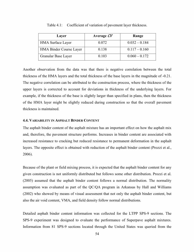
54

Table 4.1: Coefficient of variation of pavement layer thickness.

Layer Average CV Range

HMA Surface Layer 0.072 0.032 – 0.184

HMA Binder Course Layer 0.138 0.117 – 0.160

Granular Base Layer 0.103 0.060 – 0.172

Another observation from the data was that there is negative correlation between the total

thickness of the HMA layers and the total thickness of the base layers in the magnitude of -0.21.

The negative correlation can be attributed to the construction process, where the thickness of the

upper layers is corrected to account for deviations in thickness of the underlying layers. For

example, if the thickness of the base is slightly larger than specified in plans, then the thickness

of the HMA layer might be slightly reduced during construction so that the overall pavement

thickness is maintained.

4.4. VARIABILITY IN ASPHALT BINDER CONTENT

The asphalt binder content of the asphalt mixture has an important effect on how the asphalt mix

and, therefore, the pavement structure performs. Increases in binder content are associated with

increased resistance to cracking but reduced resistance to permanent deformation in the asphalt

layers. The opposite effect is obtained with reduction of the asphalt binder content (Prozzi et al.,

2006).

Because of the plant or field mixing process, it is expected that the asphalt binder content for any

given construction is not uniformly distributed but follows some other distribution. Prozzi et al.

(2005) assumed that the asphalt binder content follows a normal distribution. The normality

assumption was evaluated as part of the QC/QA program in Arkansas by Hall and Williams

(2002) who showed by means of visual assessment that not only the asphalt binder content, but

also the air void content, VMA, and field density follow normal distributions.

Detailed asphalt binder content information was collected for the LTPP SPS-9 sections. The

SPS-9 experiment was designed to evaluate the performance of Superpave asphalt mixtures.

Information from 81 SPS-9 sections located through the United States was queried from the

55

LTPP database for asphalt binder content information. For each of the SPS-9 the number of

asphalt binder observations ranged from 24 to 50. Figure 4.11 shows a typical cumulative

distribution for asphalt binder content for an asphalt layer from the SPS-9 sections. The figure

also displays a normal distribution with mean and standard deviation equal to that observed for

the same pavement section. It can be expected that the asphalt binder data for the pavement

section is likely to come from a normal distribution.

Figure 4.11: Asphalt binder content distribution for LTPP section 29-0962.

The number of asphalt binder observations for each location is still large enough to test the

hypothesis that the data follow a normal distribution using the SK statistic (H0 : the observed

asphalt binder contents follows a normal distribution against H1: the observed asphalt binder

contents do not follow a normal distribution). A significance level of 0.01 was selected to

perform the SK goodness-of-fit tests and evaluate the previous hypothesis. It was found that

85.2% of the HMA layers have asphalt content distributions that follow a normal distribution.

0

0.1

0.2

0.3

0.4

0.5

0.6

0.7

0.8

0.9

1

3.5 3.7 3.9 4.1 4.3 4.5 4.7 4.9 5.1 5.3 5.5

Cu

mm

ula

tive

Den

sity

Fun

ctio

n

Asphalt Binder Content (%)

Normal Distribution

Actual Data

Critical Tail

56

The spread of the asphalt binder content distribution was also evaluated for the pavement

sections that were used. The coefficients of variation (CV) for the analyzed asphalt layers were

found to be 0.063 on average. The CV ranged from 0.009 to 0.392.

4.5. VARIABILITY IN AIR VOID CONTENT

As with the asphalt binder content, the air void content is a volumetric property of the asphalt

mixture that has significant effect on how the asphalt mix performs. The asphalt binder content is

closely related to the compaction effort applied during construction and, therefore, is also related

to the density of the asphalt mix. It has been demonstrated that very low air voids (< 4%) can be

associated with flushing of the asphalt binder and permanent deformation on the asphalt layers

because of reduced capacity to absorb high shear stresses due to traffic loading. On the other

hand, for high air void contents, proper permeability and drainage needs to be ensured.

Otherwise, water might become trapped in the air voids causing stripping of the asphalt binder

from the aggregate particles and increase in the stress state due to hydrostatic pressure.

Due to heterogeneity in the compaction process, it is expected that the air void content for any

given construction is not uniformly distributed but follows a different distribution. Previous

researchers have also assumed normality of the air void content; this is the case of Chakroborty

et al. (2010) who showed that, based on the Marshall Method, air void content, VMA, stability

and flow follow normal distributions.

The LTPP study collected air void content information for all the flexible SPS sections and for

many of the GPS sections. Information from 194 pavement sections located through the United

States was queried from the LTPP database for air void content information (the pavement

sections with less than 5 observations were dropped from the analysis). These censoring of the

information will not introduce any biases. For each of the pavement sections the number of air

void content observations ranged from 6 to 17.

57

Figure 4.12: Air void content distribution for LTPP section 26-0114.

Figure 4.12 shows a typical distribution for air void content for an asphalt layer from the SPS-1

sections. The figure also displays a normal distribution with mean and standard deviation equal

to that observed for the same pavement section. Although the number of observations is lower

than the ones used for determining the normality of layer thickness and asphalt content, it is still

feasible to visually assess that data are likely to come from a normal distribution.

Because of the number of air void content observations for each location, the hypothesis that the

data follow a normal distribution was evaluated using the SF goodness-of-fit tests (H0: normal

against H1: not normal). A significance level of 0.01 was selected to perform the SF goodness-of-

fit tests and evaluate the previous hypothesis. It was found that 98.8% of the HMA layers have

air void content distributions that follow a normal distribution.

The spread of the air void content distribution was also evaluated for the pavement sections that

were used. The CVs for the analyzed asphalt layers were found to be 0.051 on average. The CV

0

0.1

0.2

0.3

0.4

0.5

0.6

0.7

0.8

0.9

1

5.5 6.0 6.5 7.0 7.5 8.0 8.5 9.0

Cu

mm

ula

tive

Den

sity

Fu

ncti

on

Air Void Content (%)

Normal Distribution

Actual Data

Critical Lower Tail

Critical Upper Tail

58

ranged from 0.009 to 0.390. It can be noted that the CV range is almost identical to that of asphalt

binder content. Another important observation from the data was that there is a negative

correlation between the asphalt binder content and the air void content in the order of -0.18. The

negative correlation is expected since typically higher asphalt contents allow for easier

compaction, and therefore, lower air void contents. Furthermore, for a fixed volume, the higher

the asphalt binder content, the more air void space that will be filled asphalt binder.

4.6. VARIABILITY IN MODULUS OF UNBOUND MATERIAL LAYERS

The modulus of the supporting layers has historically been considered as one of the most

important factors in pavement design and for determining the performance of a pavement

structure. In fact, most of the empirical pavement design methodologies, such as the 1993

AASHTO Design Guide, rely mostly on the modulus of the different layers, and mainly the

subgrade, to characterize the strength of the pavement structure.

However, because of non-uniformity of the materials, construction process, drainage conditions,

among others, it is unrealistic to assume that the modulus of the unbound material layers (base,

subbase, and subgrade) for any pavement structure is constant. Actually, we would expect that

the modulus of the unbound layers follows a non-uniform distribution. It is the assumption in the

current analysis that the unbound material layers follow a normal distribution also. The normality

assumption is consistent with the findings by Rada and Witzcak (1981). The validity of this

assumption is now evaluated.

As part of the LTPP project, resilient modulus information for the unbound layers was collected.

This information was collected for all SPS sections and many GPS sections. Unfortunately, the

number of samples that were collected to evaluate the resilient modulus for each unbound

material layer is small, ranging from 1 to 5 samples. Consequently, only the unbound material

layers containing 5 test repetitions were selected. Based on the previous selection, information

from 1,087 untreated subgrade layers and 16 untreated base layers located through the United

States were queried from the LTPP database for resilient modulus information. The modulus of

each of the selected sections was evaluated at least at three different confining pressures.

59

Although the Shapiro-Francia goodness-of-fit test can be used to evaluate the normality of a

sample with few observations (n ≥ 4), the authors believe that a larger data set is preferred.

Therefore, sections with resilient modulus with equivalent standard deviation (± 15 psi) were

standardized and grouped together. The grouped data was then used to evaluate the normality of

the resilient modulus data of the unbound layers.

Figure 4.13 shows the distribution for resilient modulus of a subgrade layer with a mean modulus

of 13,200 psi that is representative of a SPS-1 section. Slight deviations between the observed

cumulative density function and the theoretical normal density function can be observed in the

figure, mainly towards the tails of the distribution. However, the maximum differences at the

tails are in the order of 100 psi (in the case of Figure 4.13), which can be considered negligible

Figure 4.13: Resilient modulus distribution for a subgrade layer with mean 13,200 psi.

Because of the number of resilient modulus observations for each location, the hypothesis that

the data follow a normal distribution was evaluated using the SF goodness-of-fit tests (H0:

0

0.1

0.2

0.3

0.4

0.5

0.6

0.7

0.8

0.9

1

12,500 12,750 13,000 13,250 13,500 13,750 14,000

Cu

mm

ula

tive

Den

sity

Fu

nct

ion

Resilient Modulus (psi - 2 psi Confining Pressure)

Normal Distribution

Actual Data

Critical Tail

60

normal against H1: not normal distribution). A significance level of 0.01 was again selected to

perform the SF goodness-of-fit tests and evaluate the previous hypothesis. It was found that for

99.5% of the untreated subgrade layers and for 100.0% of the untreated base layers the resilient

modulus is likely to follow a normal distribution.

The spread of the resilient modulus distributions was also evaluated for the pavement sections

that were used. The CVs for the analyzed subgrade layers were found to be on average 0.093 and

0.101 for the analyzed subgrade and base layers respectively. A detailed summary of the CV for

the analyzed pavement layers is shown in Table 4.2. Another observation from the data was that

there is considerable positive correlation between the modulus of the base and the subgrade in

the order of 0.32. The reason for the high degree of correlation between the modulus of the base

and subgrade layers might be explained by similarity in materials, and more importantly, by

similarities in moisture content and confinement.

Table 4.2: Coefficient of variation of unbound layer resilient modulus.

Layer Average CV Range

Unbound Base Layer 0.101 0.008 – 0.370

Unbound Subgrade Layer 0.093 0.000 – 0.896

4.7. VARIABILITY IN MODULUS OF HMA LAYERS

Although not directly addressed in the present study, the variability in the modulus of the HMA

layers was also evaluated for completeness. A higher level of uniformity in the modulus of the

HMA layer because of higher QC/QA both during production and construction can be expected.

As in the case of the modulus of the unbound layers, it was initially assumed that the resilient

modulus of the HMA layers follows a normal distribution. The validity of this assumption is

evaluated next.

As part of the LTPP project, resilient modulus information for the HMA layers was also

collected. This information was collected for all flexible SPS sections and many GPS sections. In

total, the resilient modulus of 1,137 HMA layers was collected from the LTPP sections.

61

However, as in the case of the resilient modulus of unbound materials, the number of samples

that were collected to evaluate the resilient modulus for each HMA layer is small (three

repetitions at a given test temperature temperatures). The modulus of each of the selected

sections was evaluated at a minimum of three different test temperatures.

Because of the small sample size, the use of a goodness-of-fit test to evaluate the normality of

the data is not feasible. Consequently, a similar approach to that used to evaluate the normality of

the resilient modulus of unbound layers was also used. Sections with resilient modulus with

equivalent standard deviation (± 10 ksi) were standardized and grouped together. The grouped

data was then used to evaluate the normality of the resilient modulus data of the unbound layers.

Figure 4.8 shows the distribution for resilient modulus of an HMA layer with a mean modulus of

750 ksi that is representative of a SPS-9 section. It is clear from the figure that the data do not

follow a normal distribution. Based on visual inspection, most of the sections tend to follow a

uniform distribution that should not be surprising because of the tighter quality control applied

when producing the HMA mix. The theoretical uniform distribution is shown in Figure 4.14. It

can be seen that the deviations from the theoretical distribution are at a maximum under 2 ksi,

which is negligible when compared to the magnitude of the resilient modulus of an HMA layer.

Consequently, a uniform distribution seems to be an appropriate assumption for the HMA

resilient modulus data.

62

Figure 4.14: Resilient modulus distribution for a HMA layer with mean 750 ksi.

The spread of the resilient modulus distributions was also evaluated for the pavement sections

that were used. The CVs for the analyzed HMA layers were found to be on average 0.028.

However, the CV ranged from 0.002 to 1.645, indicating a great degree of variation from the

mean in some cases.

4.8. VARIABILITY SUMMARY

One of the objectives of this chapter is to highlight the impact of field variability of some

important design variables on the performance of the pavement structure as predicted by the

MEPDG. Most design and analysis tools for pavement structures assume that the input or design

parameters are deterministic or fixed, usually at the mean or average value of the distribution.

However, it has been shown that this assumption is rather unrealistic because typical variability

of the design variables will result in considerable performance variations.

0

0.1

0.2

0.3

0.4

0.5

0.6

0.7

0.8

0.9

1

600 610 620 630 640 650 660 670 680 690 700 710 720 730 740 750 760 770 780 790 800

Cu

mm

ula

tive

Den

sity

Fu

nct

ion

Resilient Modulus (ksi - 80.6oF)

Uniform Distribution

Normal Distribution

Actual Data

Critical Tail

63

When analyzing the variability and distributions of several design variables in the field

(thickness of the HMA layer, asphalt binder content, air void content, thickness of the base and

subbase layers, resilient modulus of the HMA layer, modulus of the base, and modulus of the

subgrade), it was identified that some of these variables have considerable variation. This was

especially true in the case of the thickness and the resilient modulus of the different layers. Even

though for several of these variables the average coefficients of variation were not large (under

10%), it was found that the spread of their distributions was considerable, mainly in the case of

the modulus of the HMA layer, a variable that has a deep impact on the performance of the given

layer.

Therefore, because of the variability associated with the design variables, it is strongly advised

that the analysis or design of the pavement structure be not only performed based on the mean

design values (which would only indicate what is the average performance of the given

pavement structure), but at several other critical values of the variables that are expected to have

a higher impact on the performance of the pavement structure. This can be achieved by means of

a simple sensitivity analysis of one or more of the design parameters in question, or ideally by

means of simulation in order to capture the correlation between several of these factors.

Finally, the information contained in the current chapter is based on information based on a large

sample of pavements sections from FHWA’s LTPP database. It is believed that this information

represents typical field variability and is representative of design and construction practice in the

United States.

64

65

CHAPTER 5: RELIABILITY ANALYSIS USING THE MEPDG

The following chapter describes a framework and application of the techniques described in

Chapter 3 to estimate the reliability of a pavement structure. The reliability analysis is based on

the rutting of the HMA layers, as estimated by the MEPDG.

As has been previously highlighted, the definition of failure is very important, and in most cases,

small variations can be translated into considerable changes of the probability of failure and

reliability of the pavement structure being analyzed. Therefore, to be consistent with NCHRP

(2008), and with the default values recommended by the MEPDG, for the following analysis a

pavement structure is going to be considered as failed once the HMA layer exceeds 0.25 in of

rutting after 17 years of service life.

5.1. SELECTION OF RANDOM VARIABLES

The initial step in the reliability analysis consists of determining which variables are to be

considered random (although, strictly speaking, most of them are), and to determine if the

various random variables are uncorrelated or if there is correlation to be considered between

different random variables. After this step, a reliability analysis of a given pavement structure,

based on the analysis and deterioration models from the MEPDG for a given set of conditions

can be performed.

As was indicated in Chapter 4, treating all the variables required for a complete MEPDG analysis

(Level 1, 2, or 3 input requirements) as random would be unfeasible and perhaps unnecessary for

a reasonable reliability analysis. For this reason, a sensitivity analysis was performed in the

previous chapter to determine which variables are important in evaluating the performance of a

pavement structure as per the MEPDG. The random variables that were selected in the previous

chapter, along with their coefficients of variation based on LTPP data are presented in Table 5.1.

66

Table 5.1: Pavement design variables to be treated as random parameters.

Parameter CV

HMA Thickness (in) 0.072

Asphalt Binder Content (%) 0.063

Air Voids (%) 0.051

Base Thickness (in) 0.103

Base Modulus (psi) 0.101

Subgrade Modulus (psi) 0.093

In addition to the determination of the variation of the previous variables, the LTPP database also

allowed the estimation of i) the correlation coefficient between the thickness of the HMA layer

and the thickness of the base layer (-0.21); ii) the correlation coefficient between the modulus of

the base and the subgrade (0.32); and iii) the correlation coefficient between the asphalt binder

content and the air void content (-0.18). Furthermore, based on the goodness-of-fit tests that

where performed in Chapter 4, the previous set of variables has been assumed to be normally

distributed.

5.2. DEFINITION OF PAVEMENT SECTIONS TO BE ANALYZED

As previously discussed, the current analysis focuses on the reliability of a pavement structure as

measured by rutting of the HMA layers. Because of the significant influence of temperature and

weather on rutting, three of the original Strategic Highway Research Program (SHRP) climatic

zones used in the development of the Superpave Ndesign table have been selected (Cominsky et

al., 1994; Prowell and Brown, 2007): a cold climatic region (Salem, OR), a warm climate region

(Destin, FL) and a hot climatic region (Imperial, CA). The locations of the three climatic regions

that have been selected are shown in Figure 5.1. The climatic data was obtained from the

MEPDG v1.0 Enhanced Integrated Climatic Model (EICM)2. The depth to water table was

assumed constant for the three climatic conditions, and equal to 8 ft. This depth to water table

corresponds to the median value for the continental United States based on the LTPP dataset.

2 The EICM is a climatic database containing hourly data for 800 weather stations from across the United States, and includes measures of sunshine, rainfall, wind speed, air temperature, and relative humidity. The climatic data has been obtained from the National Climate Data Center (NCDC).

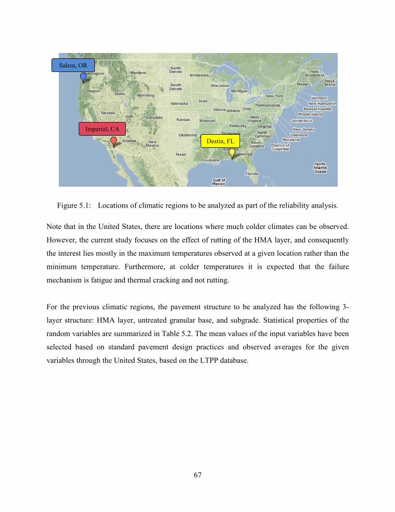
67

Figure 5.1: Locations of climatic regions to be analyzed as part of the reliability analysis.

Note that in the United States, there are locations where much colder climates can be observed.

However, the current study focuses on the effect of rutting of the HMA layer, and consequently

the interest lies mostly in the maximum temperatures observed at a given location rather than the

minimum temperature. Furthermore, at colder temperatures it is expected that the failure

mechanism is fatigue and thermal cracking and not rutting.

For the previous climatic regions, the pavement structure to be analyzed has the following 3-

layer structure: HMA layer, untreated granular base, and subgrade. Statistical properties of the

random variables are summarized in Table 5.2. The mean values of the input variables have been

selected based on standard pavement design practices and observed averages for the given

variables through the United States, based on the LTPP database.

Salem, OR

Imperial, CA

Destin, FL

68

Table 5.2: Mean and standard deviation for random design variables.

Parameter Mean Std. Dev.

HMA Thickness (in) 4.5 / 10.0 0.33 / 0.72

Asphalt Binder Content (%) 5.0 0.32

Air Voids (%) 7.0 0.36

Base Thickness (in) 14.0 1.44

Base Modulus (psi) 22,000 2222

Subgrade Modulus (psi) 10,000 930

As can be observed from Table 5.2, two different thicknesses for the HMA layer were selected.

This has been done because the performance and the deterioration patterns of HMA layers vary

significantly for thin and thick asphalt layers. This is due to the considerable difference in stress

distribution which is determined by the relationship between the tire size and the layer thickness.

Thin pavements are considered those whose thickness is in the order (or thinner) that the radius

of the tire-pavement contact area. When the contact radius is considerably smaller than the

thickness of the layer, the layer is considered thick.

The distinction is important since in the case of thin HMA layers, the wheel tire provides

confining producing a shear effect on the HMA layer, while in the case of thick HMA layers, the

layer is allowed to fully develop tension at the bottom. Therefore, the effect of differences in

performance and reliability of the pavement structure in thin and thick HMA layers as

determined by the MEPDG can be analyzed.

5.2.1. Traffic Loading

Two types of truck traffic distributions have been included in the reliability analysis. The traffic

classifications are based on the truck classification system that is used in the MEPDG (Figure

5.2). The selected traffic distributions are intended to capture the effect of single-unit trucks

(typical of urban traffic) and single-trailer trucks (typical of rural traffic).

69

Figure 5.2: Truck Traffic Classes included in the MEPDG (from NCHRP, 2004).

Based on the previous classification, the traffic was assumed to follow either a Type 2 Truck

Traffic Classification (TTC 2) which consists “predominantly of single-trailer trucks with a low

percentage of single-unit trucks” or a Type 12 Truck Traffic Classification (TTC 12) which

corresponds to “mixed truck traffic with a higher percentage of single-unit trucks” (NCHRP,

2004). The TTC2 type traffic corresponds to typical rural truck traffic conditions, while TTC12

traffic can be mostly associated with typical urban truck traffic.

Both the TTC 2 and TTC 12 distributions included more than 2% buses and less than 2% multi-

trailer trucks. The two selected TTC are shown in Figures 5.3 and 5.4.

Figure 5.3: Type 2 Truck Traffic Classification.

0

10

20

30

40

50

60

70

Per

cen

tage

(%)

TTC 2

70

Figure 5.4: Type 12 Truck Traffic Classification.

As for daily truck traffic, the average annual daily truck traffic (AADTT) was selected in such a

way that the limiting acceptable values of rutting were reached (while holding all other design

inputs variables constant) after a 20 year analysis period (note that this is different to the design

period of 17 years). From Figures 5.5 thru 5.8, the critical AADTT values (for 0.25 in. rutting)

can be determined for the cold, warm, and hot climatic regions, for both thin (4.5 in) and thick

(10.0 in) HMA layers. The figures clearly show that warmer climates are more prone to rutting

than cooler climates. This is expected because of the visco-elastic behavior of the asphalt binder

(softer at high temperatures and stiffer at lower temperatures). It can also be observed from the

figures that TTC 2 generates more rutting on the HMA layers, as compared to TTC 12, for equal

amounts of truck traffic. Table 5.3 summarizes the critical AADTT values that have been

selected as design traffic for the following analysis.

0

10

20

30

40

50

60

70P

erce

nta

ge (%

)TTC 12

Figure 5.5: Effect of traffic on


71

n rutting of the HMA layer (4.5 in HMA layer, TT

rutting of the HMA layer (4.5 in HMA layer, TTC

TC 2).

C 12).


Figure 5.8: Effect of traffic on r

72

rutting of the HMA layer (10.0 in HMA layer, TT

rutting of the HMA layer (10.0 in HMA layer, TT

TC 2).

TC 12).

73

Table 5.3: Critical AADTT values to ensure 0.25 in of rutting on the HMA layer.

Climatic

Region

AADTT

4.5 in HMA Layer 10.0 in HMA Layer

TTC 2 TTC 12 TTC 2 TTC 12

Cold 3,294 4,742 9,506 13,944

Warm 687 1,000 1,846 2,738

Hot 325 500 736 1,090

5.3. DEVELOPMENT OF 1-DEGREE RESPONSE SURFACES FOR RUTTING PERFORMANCE

Response surfaces are used in the following analysis of the reliability of pavement structures.

The response surfaces will be used to represent the rutting, in inches, of the HMA layer as

predicted by the MEPDG.

In order to fit the rutting models, the MEPDG was run a total of 729 times based on all the

combinations of the following values of the selected random variables (full factorial, 36):

• HMA Thicknesses (HMA): mean, – 1 SD, – 2 SD. • Asphalt Binder Content (BC): mean, + 1 SD, + 2 SD. • Air Voids (AV): mean, – 2 SD, + 2 SD. • Base Thickness (Base): mean, – 1 SD, – 2 SD. • Base Modulus (MRb): mean, – 1 SD, – 2 SD. • Subgrade Modulus (MRs): mean, – 1 SD, – 2 SD.

where SD denotes standard deviation. The previous selection of ± 1 SD and ± 2 SD was made on

the assumption that moving in the indicated direction of the random variable, the probability of

failure of the pavement structure will increase.

All the previous combinations of random variables were evaluated using the MEPDG (aiming

for a 90% reliability target, which on average corresponded to a 17 year design period) at the

three selected climatic regions (cool, warm, and hot), two truck traffic distributions (TTC 2 and

TTC 12), and two significantly different thickness of the HMA layer (4.5 in and 10.0 in). Based

74

on all of the 8,748 combinations of the factorial experiment (729 · 12), the HMA rutting model

response surfaces can be developed.

It is likely that a linear regression model based on the preceding random variables should

properly capture the rutting of the HMA layer. This is expected since the modeling of the

response surface has been done on a small area around the design point (mean values of random

design inputs). The linearity of rutting of the HMA layer as a function of some of the random

parameters (air void content and asphalt content) can be observed in Figure 5.9 and 5.10. From

the figures, it can be visually assessed that an initial linear estimation might be appropriate.

Figure 5.9: Effect of air void content on rutting of a 10.0 in HMA layer in a Warm Climatic

Region (TTC 2).

0.245

0.250

0.255

0.260

0.265

0.270

0.275

6.6 6.7 6.8 6.9 7.0 7.1 7.2 7.3 7.4

HM

A R

utt

ing

(in

)

Air Void Content (%)

75

Figure 5.10: Effect of asphalt binder content on rutting of a 4.5 in HMA layer in a Hot Climatic

Region (TTC 2).

However, apart from the highly linear behavior of some of the design variables within the

analysis range, some slight curvature has also been observed in the prediction of rutting in the

HMA layer by other of the input design variables, such as modulus of the base layer (Figure

5.11). Note that the curvature is small given the wide range of modulus of the base layer that was

captured. To address this nonlinearity of the HMA rutting predictions due to some of the input

design variables, second-order polynomials will also be used at a later stage to improve the fit of

the response surfaces and account for the curvature in the reliability estimates.

0.685

0.690

0.695

0.700

0.705

0.710

0.715

4.9 5.0 5.1 5.2 5.3 5.4 5.5 5.6

HM

A R

utt

ing

(in

)

Asphalt Binder Content (%)

76

Figure 5.11: Effect of base modulus on rutting of a 4.5 in HMA layer in a Hot Climatic Region

(TTC 12).

The initial response surfaces consists of a linear approximation to the rutting as

determined by the MEPDG, and can be represented in mathematically as follows, = + + + + + + + [5.1]

Where represents the rutting on the HMA layer after 17 years of service life in

inches and corresponds to a disturbance term or random variable that accounts for unobserved

factors that affect the rutting process of the HMA layer. The subindex indicates each possible

combination of truck traffic loading, environment, and thickness type of the HMA layer.

The detailed parameter estimates and standard errors are presented in the following tables.

0.24

0.25

0.26

0.27

0.28

0.29

0.30

0 5,000 10,000 15,000 20,000 25,000

HM

A R

utt

ing

(in

)

Modulus of Base Layer (psi)

77

Table 5.4: Parameter estimates for rutting of HMA layer in Cool Climatic Region.

Parameter (Std. Dev.)

t-statParameter (Std. Dev.)



t-stat

Intercept0.481

(0.007)65.2

0.473 (0.007)

65.0-0.017 (0.002)

-7.9-0.016 (0.002)

-7.4

HMA-0.088

(0.60x10-3)-145.6

-0.086 (0.59x10-3)

-144.9-0.007

(0.08x10-3)-87.3

-0.007 (0.08x10-3)

-85.1

Base1.39x10-4

(1.46x10-4)1.0

1.58x10-4 (1.44x10-4)

1.112.03x10-4 (0.43x10-4)

27.912.04x10-4 (0.43x10-4)

27.8

MRb-2.40x10-6 (3.91x10-8)

-61.4-2.33x10-6 (3.85x10-8)

-60.61.22x10-6

(1.15x10-8)105.8

1.22x10-6 (1.15x10-8)

106.0

MRs-1.25x10-6 (1.24x10-7)

-10.1-1.33x10-6 (1.22x10-7)

-10.82.50x10-6

(3.68x10-7)67.8

2.32x10-6 (3.69x10-7)

63.1

BC0.018

(0.78x10-3)23.6

0.018 (0.77x10-3)

23.40.023

(0.23x10-3)101.2

0.023 (0.23x10-3)

99.9

AV0.015

(0.73x10-3)20.4

0.015 (0.72x10-3)

20.20.019

(0.22x10-3)87.7

0.019 (0.22x10-3)

86.6

R 2

σ

0.982 0.982 0.989 0.988

0.004 0.004 0.001 0.001

Variable

4.5 in HMA Layer 10.0 in HMA LayerTTC 2 TTC 12 TTC 2 TTC 12

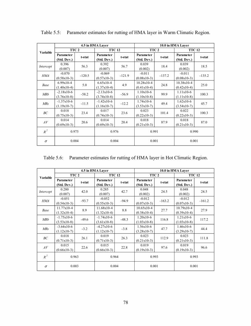
78

Table 5.5: Parameter estimates for rutting of HMA layer in Warm Climatic Region.

Table 5.6: Parameter estimates for rutting of HMA layer in Hot Climatic Region.





t-stat

Intercept0.396

(0.007)56.3

0.392 (0.007)

56.70.039

(0.002)18.4

0.039 (0.002)

18.5

HMA-0.070

(0.58x10-3)-120.5

-0.069 (0.57x10-3)

-121.9-0.011

(0.08x10-3)-137.2

-0.011 (0.08x10-3)

-135.2

Base6.99x10-4

(1.40x10-4)5.0

6.65x10-4 (1.37x10-4)

4.910.28x10-4 (0.41x10-4)

24.810.38x10-4 (0.42x10-4)

25.0

MRb-2.18x10-6 (3.76x10-8)

-58.2-2.13x10-6 (3.74x10-8)

-56.91.10x10-6

(1.10x10-8)99.9

1.11x10-6 (1.11x10-8)

100.3

MRs-1.37x10-6 (1.19x10-7)

-11.5-1.42x10-6 (1.16x10-7)

-12.21.74x10-6

(3.53x10-7)49.4

1.62x10-6 (3.54x10-7)

45.7

BC0.018

(0.75x10-3)23.4

0.017 (0.74x10-3)

23.60.023

(0.22x10-3)101.4

0.022 (0.22x10-3)

100.3

AV0.014

(0.69x10-3)20.6

0.014 (0.69x10-3)

20.40.018

(0.21x10-3)87.9

0.018 (0.21x10-3)

87.0

R 2

σ

0.975 0.976 0.991 0.990

0.004 0.004 0.001 0.001

Variable






t-stat

Intercept0.280

(0.007)42.0

0.285 (0.007)

42.70.048

(0.002)24.5

0.048 (0.002)

24.5

HMA-0.051

(0.54x10-3)-93.7

-0.052 (0.55x10-3)

-94.9-0.012

(0.07x10-3)-163.2

-0.012 (0.07x10-3)

-161.2

Base11.77x10-4 (1.32x10-4)

8.911.68x10-4 (1.32x10-4)

8.810.65x10-4 (0.38x10-4)

27.710.79x10-4 (0.39x10-4)

27.9

MRb-1.75x10-6 (3.53x10-8)

-49.6-1.74x10-6 (3.61x10-8)

-48.31.20x10-6

(1.03x10-8)116.8

1.21x10-6 (1.03x10-8)

117.2

MRs-3.64x10-6 (1.12x10-7)

-3.2-4.27x10-6 (1.12x10-7)

-3.81.56x10-6

(3.28x10-7)47.7

1.46x10-6 (3.29x10-7)

44.4

BC0.018

(0.71x10-3)26.1

0.019 (0.71x10-3)

26.30.023

(0.21x10-3)112.9

0.023 (0.21x10-3)

111.8

AV0.015

(0.66x10-3)22.6

0.015 (0.66x10-3)

22.80.019

(0.19x10-3)97.6

0.019 (0.19x10-3)

96.6

R 2

σ

0.963 0.964 0.993 0.993

0.003 0.004 0.001 0.001

Variable


79

It can be observed from Tables 5.4 thru 5.6 that most of the parameters are significant at a five

percent level. The exception is the thickness of the base layer for predicting the rutting of a thin

HMA layer (4.5 in) on a Cold Climatic Region. However, the variable has not been dropped

from the analysis since it has been found to be jointly significant (with the other input variables)

in the prediction of HMA rutting.

It can also be observed from the previous tables that the fit of the response surfaces, as measured

by R2, is very good and for all scenarios greater than 96%. It was also noted that the efficiency of

the models increases when the thickness of the HMA layer is increased from 4.5 in to 10.0 in.

This can be corroborated by the reduction in model standard error associated with the change in

HMA layer thickness (approximately from 3 to 4 times reduction).

Finally, based on the previously estimated response surfaces ([5.1] and Tables 5.4 thru 5.6), the

limit state function for rutting of the HMA layer (in inches) can be defined as follows, ( , , , , , , ) = 0.25 − [5.2]

As previously mentioned, the 0.25 in threshold for HMA layer rutting corresponds to the default

failure criterion in the MEPDG. Additionally, note that in order to account for unobserved

factors that affect rutting, a disturbance term ( ) has also been introduced in (∙) as a

normal random variable with mean zero and standard deviation equal the standard error

associated to each respective model.

5.4. FORM ANALYSIS BASED ON 1-DEGREE RESPONSE SURFACE

FORM was performed assigning the variability presented in Table 5.1 to the different input

parameters. Additionally, the parameters are not assumed independent but correlated as per

Section 5.1. Furthermore, based on the analysis performed on Chapter 4, the input variables have

been assumed normally distributed with mean values as per Table 5.2.

The results from FORM, using the limit state function [5.2] are shown in Tables 5.7 thru 5.9.

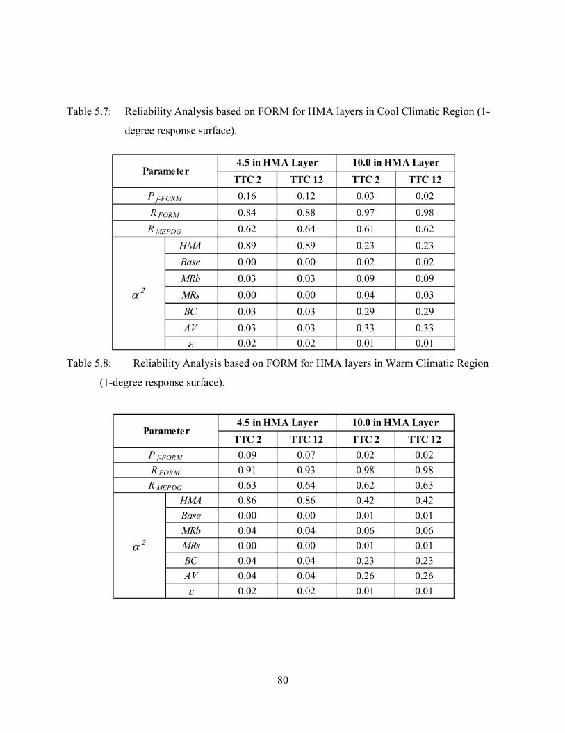
80

Table 5.7: Reliability Analysis based on FORM for HMA layers in Cool Climatic Region (1-

degree response surface).

Table 5.8: Reliability Analysis based on FORM for HMA layers in Warm Climatic Region

(1-degree response surface).


0.16 0.12 0.03 0.02

0.84 0.88 0.97 0.98

0.62 0.64 0.61 0.62

HMA 0.89 0.89 0.23 0.23

Base 0.00 0.00 0.02 0.02

MRb 0.03 0.03 0.09 0.09

MRs 0.00 0.00 0.04 0.03

BC 0.03 0.03 0.29 0.29

AV 0.03 0.03 0.33 0.33

ε 0.02 0.02 0.01 0.01


P f-FORM

R FORM

R MEPDG

α 2

Parameter


0.09 0.07 0.02 0.02

0.91 0.93 0.98 0.98

0.63 0.64 0.62 0.63

HMA 0.86 0.86 0.42 0.42

Base 0.00 0.00 0.01 0.01

MRb 0.04 0.04 0.06 0.06

MRs 0.00 0.00 0.01 0.01

BC 0.04 0.04 0.23 0.23

AV 0.04 0.04 0.26 0.26

ε 0.02 0.02 0.01 0.01

R MEPDG

α 2

Parameter4.5 in HMA Layer 10.0 in HMA Layer

P f-FORM

R FORM

81

Table 5.9: Reliability Analysis based on FORM for HMA layers in Hot Climatic Region (1-

degree response surface).

The tables show the probability of failure and reliability of the different pavement structures that

have been analyzed estimated directly from the MEPDG, and using FORM based on [5.2]. Based on FORM it can be observed that for all of the analyzed scenarios, the reliability as

estimated directly by the MEPDG is very conservative, an approximately 20% to 30% lower

than the FORM estimates.

The probabilities of failure, as estimated by FORM are in the order of 2% to 16% (as opposed to

the MEPDG estimates of approximately 40%). However, it is important to note that because this

is a linear deterioration function with normal random variables, the probability of failure using

FORM would only be exact if [5.1] were the true model for predicting failure.

FORM analysis also has the advantage that it provides some additional information on the

influence of each random variable on the probability of failure of the pavement structure (based

on rutting of the HMA layer as the failure criterion). The squared directional cosines ( ) of the

reliability index in the standard normal space (refer to Figure 3.1) provide an indication of the

TTC 2 TTC 12 TTC 2 TTC 120.07 0.09 0.09 0.07

0.93 0.91 0.91 0.93

0.61 0.60 0.59 0.60

HMA 0.78 0.78 0.45 0.45

Base 0.01 0.01 0.01 0.01

MRb 0.04 0.04 0.05 0.05

MRs 0.00 0.00 0.01 0.01

BC 0.07 0.06 0.22 0.22

AV 0.07 0.07 0.24 0.25

ε 0.03 0.03 0.01 0.01

R MEPDG

α 2


P f-FORM

R FORM

82

relative importance of the random variables on the reliability index and, therefore, on the

probability of failure. In the analysis of failure using the response surface, the

squared directional cosines ( ) indicate that for the case of thin HMA layers (4.5 in scenario)

the most significant variable that influences the reliability of the pavement structure is the

thickness of the HMA structure. Also note that the relative importance of thickness of the HMA

layer decreases as the temperature increases (over 10% decrease for the evaluated climatic

range). Additionally, the modulus of the base layer and the volumetric properties of the HMA

mix (air void content and asphalt binder content) also have an important effect on the probability

of failure.

In the case of pavements with thick HMA layers (10.0 in scenario), the thickness of the HMA

layer continues to be one of the most important factors in determining the failure of the pavement

structure. It can also be noted that as opposed the thin HMA layer scenario (4.5 in scenario), the

effect of the thickness of the HMA layer increases as the temperature decreases (over 20%

increase for the evaluated climatic range). Also, in the case of thick HMA layers, the volumetric

properties of the asphalt mixture ( , ) have a similar or higher impact to the thickness of the

HMA layer on the deterioration of the pavement structure. The effect of the remaining variables

also increases, as compared to the thin HMA layer case.

5.5. SIMULATION ANALYSIS BASED ON 1-DEGREE RESPONSE SURFACE

As an alternate means of estimating reliability based on the 1-degree limit state function defined

in [5.2] (∙) simulation was performed. The simulation results can also be used as a

means of verifying the results obtained from FORM.

Simulation was performed using the Crude Monte Carlo and Latin Hypercube based on a sample

size of 10,000 runs and 10 repetitions. It is expected that the Latin Hypercube estimates are more

efficient and converge faster. Additionally, in order to further validate the results, Crude Monte

Carlo simulation was also performed increasing the sample size to 1,000,000 and performing 50

repetitions.

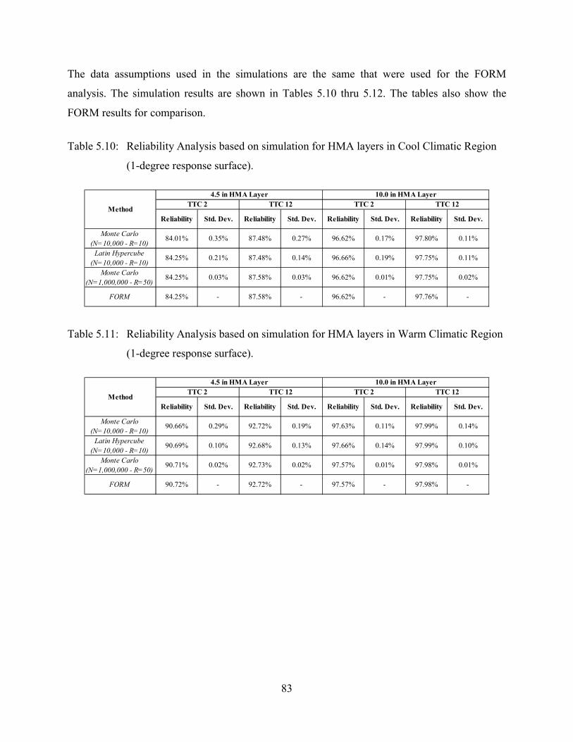
83

The data assumptions used in the simulations are the same that were used for the FORM

analysis. The simulation results are shown in Tables 5.10 thru 5.12. The tables also show the

FORM results for comparison.

Table 5.10: Reliability Analysis based on simulation for HMA layers in Cool Climatic Region


Table 5.11: Reliability Analysis based on simulation for HMA layers in Warm Climatic Region


Reliability Std. Dev. Reliability Std. Dev. Reliability Std. Dev. Reliability Std. Dev.

Monte Carlo (N=10,000 - R=10)

84.01% 0.35% 87.48% 0.27% 96.62% 0.17% 97.80% 0.11%

Latin Hypercube (N=10,000 - R=10)

84.25% 0.21% 87.48% 0.14% 96.66% 0.19% 97.75% 0.11%

Monte Carlo (N=1,000,000 - R=50)

84.25% 0.03% 87.58% 0.03% 96.62% 0.01% 97.75% 0.02%

FORM 84.25% - 87.58% - 96.62% - 97.76% -

Method




90.66% 0.29% 92.72% 0.19% 97.63% 0.11% 97.99% 0.14%


90.69% 0.10% 92.68% 0.13% 97.66% 0.14% 97.99% 0.10%

Monte Carlo (N=1,000,000 - R=50)

90.71% 0.02% 92.73% 0.02% 97.57% 0.01% 97.98% 0.01%

FORM 90.72% - 92.72% - 97.57% - 97.98% -

Method


84

Table 5.12: Reliability Analysis based on simulation for HMA layers in Hot Climatic Region


The tables show the reliability estimates based on simulation using the (∙) limit state

function are consistent with the FORM estimates. It can also be noted that all the reliability

estimates based on simulation are also consistent among themselves. However, it is clear that for

a fixed sampling number (10,000) and number of repetitions (10) the Crude Monte Carlo method

is associated with higher variation in the estimates (on average the standard error based on Latin

Hypercube is 80% of that obtained using Crude Monte Carlo). Because of the previous reason,

the rate of conversion using Crude Monte Carlo is lower.

Regardless of the type of simulation performed, the standard errors obtained from all the

simulations are negligible compared to the typical magnitudes for the probability of failures

associates with pavement structures.



93.03% 0.24% 90.43% 0.27% 91.28% 0.35% 92.72% 0.17%


93.12% 0.19% 90.52% 0.19% 91.21% 0.28% 92.60% 0.17%

Monte Carlo (N=1,000,000 - R=50)

93.04% 0.02% 90.50% 0.02% 91.26% 0.03% 92.61% 0.03%

FORM 93.04% - 90.50% - 91.26% - 92.61% -

Method


85

CHAPTER 6: Correction in Reliability Estimates Due to Curvature

The reliability analysis in the previous chapter was based on the assumption that the limit state

function corresponds to a 1-degree polynomial function: (∙). The 1-degree polynomial

approximation to the limit state function was assumed as appropriate because of the relative

linearity of some of the design input variables that are addressed as part of the current study

(refer to Section 5.3). However, it was also observed that the effect of some of the variables is

not necessarily linear. Furthermore, strong correlations have been identified between several of

the analysis variables (e.g. resilient modulus of base and subbase). For this reason, a response

surface that incorporates a certain degree of nonlinearity is evaluated in the present chapter.

6.1. DEVELOPMENT OF 2-DEGREE RESPONSE SURFACES WITH INTERACTION TERMS FOR

RUTTING PERFORMANCE

The response surface to be fit in the following section was initially based on a 2-degree

polynomial function with interaction terms between all the variables for which correlation was

identified. Mathematically, the response surfaces which consists of an

approximation to the rutting of the HMA layer as determined by the MEPDG, and can be

represented in mathematically as follows, = + + + + + + ++ + + + + + ∙+ ∙ + ∙ + [6.1] where represents the rutting on the HMA layer after 17 years of service life in

inches and corresponds to a disturbance term or random variable that accounts for unobserved

factors that affect the rutting process of the HMA layer. The subindex indicates each possible

combination of truck traffic loading, environment, and thickness type of the HMA layer.

After several iterations, it was identified that the effect of several of the quadratic terms and

interaction terms were not significant (at a level of confidence of 90%) in explaining the rutting

of the HMA layer. Consequently, the non-significant parameters were dropped from the model,

and the final response surface can be expressed as follows,

86

= + + + + + + ++ ∙ + [6.2] The detailed parameter estimates and standard errors associated with [6.2] are presented in the

following tables.






t-stat

Intercept0.984

(0.048)20.7

0.967 (0.047)

20.60.192

(0.014)14.1

0.195 (0.014)

14.3

HMA-0.327

(22.82x10-3)-14.4

-0.321 (22.50x10-3)

-14.3-0.053

(2.92x10-3)-18.2

-0.053 (2.91x10-3)

-18.3

Base1.39x10-4

(1.31x10-4)1.1

1.58x10-4 (1.29x10-4)

1.212.03x10-4 (0.35x10-4)

34.312.04x10-4 (0.35x10-4)

34.4

MRb-2.92x10-6 (2.13x10-8)

-13.7-2.88x10-6 (2.10x10-8)

-13.81.30x10-6

(5.70x10-8)22.9

1.31x10-6 (5.69x10-8)

23.1

MRs-2.35x10-6 (4.59x10-7)

-5.1-2.50x10-6 (4.52x10-7)

-5.52.67x10-6

(1.22x10-7)21.8

2.51x10-6 (1.22x10-7)

20.5

BC0.018

(0.70x10-3)26.2

0.018 (0.69x10-3)

26.10.023

(0.19x10-3)124.4

0.023 (0.19x10-3)

123.3

AV0.015

(0.66x10-3)22.7

0.015 (0.65x10-3)

22.50.019

(0.18x10-3)107.9

0.019 (0.18x10-3)

106.9

HMA 2 0.029 (2.75x10-3)

10.50.028

(2.72x10-3)10.5

0.002 (0.16x10-3)

15.70.002

(0.16x10-3)15.8

MRb . MRs6.264x10-6

(2.532x10-7)2.5

6.679x10-6 (2.496x10-7)

2.7-9.906x10-6 (6.783x10-7)

-1.5-1.039x10-6 (6.767x10-7)

-1.5

R 2

σ

Variable


0.986 0.985 0.993 0.992

0.003 0.003 0.001 0.001

87






t-stat

Intercept0.854

(0.046)18.6

0.847 (0.045)

19.00.282

(0.011)24.9

0.284 (0.011)

25.0

HMA-0.285

(22.00x10-3)-12.9

-0.282 (21.37x10-3)

-13.2-0.064

(2.44x10-3)-26.3

-0.064 (2.44x10-3)

-26.4

Base6.99x10-4

(1.26x10-4)5.5

6.64x10-4 (1.23x10-4)

5.410.28x10-4 (0.29x10-4)

35.110.38x10-4 (0.29x10-4)

35.4

MRb-3.05x10-6 (2.05x10-8)

-14.9-3.01x10-6 (2.03x10-8)

-14.81.18x10-6

(4.76x10-8)24.9

1.19x10-6 (4.76x10-8)

25.1

MRs-3.20x10-6 (4.42x10-7)

-7.3-3.30x10-6 (4.35x10-7)

-7.61.90x10-6

(1.02x10-7)18.6

1.79x10-6 (1.02x10-7)

17.4

BC0.018

(0.68x10-3)26.0

0.017 (0.66x10-3)

26.30.023

(0.16x10-3)143.2

0.022 (0.16x10-3)

142.1

AV0.014

(0.62x10-3)22.8

0.014 (0.61x10-3)

22.70.018

(0.15x10-3)124.2

0.018 (0.15x10-3)

123.3

HMA 2 0.026 (2.66x10-3)

9.80.026

(2.58x10-3)10.0

0.003 (0.13x10-3)

21.80.003

(0.13x10-3)22.0

MRb . MRs1.042x10-6

(2.441x10-7)4.3

1.073x10-6 (2.420x10-7)

4.4-9.207x10-6 (5.657x10-7)

-1.6-9.618x10-6 (5.664x10-7)

-1.7

R 2

σ

Variable


0.980 0.981 0.995 0.995

0.003 0.003 0.001 0.001

88


Similar to the 1-degree response surfaces, it can be observed from Tables 6.1 thru 6.3 that most

of the parameters are significant at the five percent level. The only factor that is less significant

in some of the scenarios is the interaction factor between modulus of the base and subgrade (in

the 10.0 in thick HMA layer scenarios). However, the interaction term was not removed from the

analysis since it has been found to be jointly significant (with the other input variables) in the

prediction of HMA rutting.

Additionally, as compared to the 1-degree response surface, the fit of the models also improved

and for all scenarios it is now greater than 97% (as measured by R2). The efficiency of the

models also improved as compared to the 1-degree response surface. The trends with regard to

model standard error also remain: improved efficiency in models consisting of a thick HMA

layer (10.0 in scenarios) as measured by reduction in standard error of approximately 4.





t-stat

Intercept0.688

(0.043)15.9

0.847 (0.045)

19.00.282

(0.011)24.9

0.284 (0.011)

25.0

HMA-0.241

(20.78x10-3)-11.6

-0.282 (21.37x10-3)

-13.2-0.064

(2.44x10-3)-26.3

-0.064 (2.44x10-3)

-26.4

Base11.77x10-4 (1.19x10-4)

9.96.64x10-4

(1.23x10-4)5.4

10.28x10-4 (0.29x10-4)

35.110.38x10-4 (0.29x10-4)

35.4

MRb-2.66x10-6 (1.94x10-8)

-13.7-3.01x10-6 (2.03x10-8)

-14.81.18x10-6

(4.76x10-8)24.9

1.19x10-6 (4.76x10-8)

25.1

MRs-2.29x10-6 (4.18x10-7)

-5.5-3.30x10-6 (4.35x10-7)

-7.61.90x10-6

(1.02x10-7)18.6

1.79x10-6 (1.02x10-7)

17.4

BC0.018

(0.64x10-3)28.8

0.017 (0.66x10-3)

26.30.023

(0.16x10-3)143.2

0.022 (0.16x10-3)

142.1

AV0.015

(0.60x10-3)25.0

0.014 (0.61x10-3)

22.70.018

(0.15x10-3)124.2

0.018 (0.15x10-3)

123.3

HMA 2 0.023 (2.51x10-3)

9.20.026

(2.58x10-3)10.0

0.003 (0.13x10-3)

21.80.003

(0.13x10-3)22.0

MRb . MRs1.100x10-6

(2.306x10-7)4.8

1.073x10-6 (2.420x10-7)

4.4-9.207x10-6 (5.657x10-7)

-1.6-9.618x10-6 (5.664x10-7)

-1.7

R 2

σ

Variable


0.970 0.971 0.995 0.995

0.003 0.003 0.001 0.001

89

Then, based on the previously estimated response surfaces ([6.2] and Tables 6.1 thru 6.3), the

limit state function for rutting of the HMA layer (in inches) can now be defined as follows, ( , , , , , , ) = 0.25 − [6.3]

Again, note that in order to account for unobserved factors that affect rutting, a disturbance term ( ) has also been introduced in (∙) as a normal random variable with mean zero and

standard deviation equal the standard error associated to each respective model.

6.2. FORM AND SORM ANALYSIS BASED ON 2-DEGREE RESPONSE SURFACE WITH

INTERACTION TERMS

Based on the same data assumptions for the input factors, FORM and SORM analysis was

performed based on the 2-degree limit state function with interaction terms (∙) . The

results from FORM and SORM, using the limit state function [6.3] are shown in Tables 6.4 thru

6.6.

90

Table 6.4: Reliability Analysis based on FORM and SORM for HMA layers in Cool Climatic

Region (2-degree response surface with interaction terms).

Table 6.5: Reliability Analysis based on FORM and SORM for HMA layers in Warm Climatic



0.14 0.11 0.03 0.02

0.86 0.89 0.97 0.98

0.14 0.11 0.03 0.02

0.86 0.89 0.97 0.98

0.62 0.64 0.61 0.62

HMA 0.90 0.90 0.20 0.22

Base 0.00 0.00 0.02 0.02

MRb 0.03 0.03 0.09 0.09

MRs 0.00 0.00 0.04 0.03

BC 0.03 0.03 0.30 0.30

AV 0.03 0.03 0.34 0.34

ε 0.01 0.01 0.01 0.01

R MEPDG

R FORM


P f-FORM

P f-SORM

α 2

R SORM


0.08 0.07 0.02 0.02

0.92 0.93 0.98 0.98

0.09 0.07 0.02 0.02

0.91 0.93 0.98 0.98

0.63 0.64 0.62 0.63

HMA 0.88 0.89 0.49 0.50

Base 0.00 0.00 0.01 0.01

MRb 0.03 0.03 0.05 0.05

MRs 0.00 0.00 0.01 0.01

BC 0.03 0.03 0.20 0.20

AV 0.04 0.04 0.23 0.23

ε 0.02 0.01 0.00 0.00

R FORM


P f-FORM

R SORM

R MEPDG

α 2

P f-SORM

91

Table 6.6: Reliability Analysis based on FORM and SORM for HMA layers in Hot Climatic


As was initially assumed, the probability of failure, and hence the reliability estimates by means

of SORM are very similar to those obtained from the FORM analysis. Typically it can be

observed that the SORM estimates are approximately 1% lower than the FORM estimates.

Similar to the case of the 1-degree limit state function, the probabilities of failure, as estimated

by SORM based on the 2-degree limit state function with interaction terms are in the order of 2%

to 14% (as opposed to the MEPDG estimates of approximately 40%).

Based on the squared directional cosines ( ) from the FORM analysis similar conclusions to

those based on the 1-degree limit state function can also be made: for the case of thin HMA

layers the most significant variable that influences the reliability of the pavement structure is the

thickness of the HMA structure. However, the effect of thickness of the HMA layer decreases as

the temperature increases (up to 10% decrease in the analysis range: cool climate to hot climate).

Additionally, the modulus of the base layer and the volumetric properties of the HMA mix (air

void content and asphalt binder content) also have an effect on the probability of failure. Finally,

TTC 2 TTC 12 TTC 2 TTC 120.06 0.08 0.08 0.06

0.94 0.92 0.92 0.94

0.06 0.09 0.08 0.07

0.94 0.91 0.92 0.93

0.61 0.60 0.59 0.60

HMA 0.82 0.81 0.45 0.46

Base 0.01 0.01 0.01 0.01

MRb 0.03 0.03 0.05 0.05

MRs 0.00 0.00 0.01 0.01

BC 0.06 0.06 0.22 0.22

AV 0.07 0.07 0.25 0.25

ε 0.02 0.02 0.00 0.00


R FORM

R SORM

P f-FORM

P f-SORM

R MEPDG

α 2

92

note that the model error is also important. This indicates that there are further factors that are

currently not being considered in the limit state function that influence rutting of the HMA layer.

In the case of pavements with thick HMA layers, the thickness of the HMA layer is still one of

the most important factors in determining the failure of the pavement structure (and is higher in

warm climatic regions). It can also be observed that the effect of the thickness of the HMA layer

increases as the temperature decreases (over 30% increase for the evaluated climatic range). The

volumetric properties of the asphalt mixture ( , ) also have a very important impact on

failure of the pavement structure due to rutting of the HMA layer. The effect of the remaining

variables also increases, as compared to the thin HMA layer case.

6.3. ELASTICITY ANALYSIS

In the previous section, the effect of the different variables on the probability of failure or

reliability of a pavement section by means of the directional cosines ( ) was evaluated.

However, as was mentioned before, the conclusions extracted from the directional cosines are

based on the assumption that all of the variables are independent. This is clearly not the case

because of the strong correlations between some of the evaluated parameters.

For the previous reason, it is important to understand what the effect on reliability is when one of

the input variables is changed. This type of sensitivity analysis can be performed based on the

elasticity of the different variables. In this case, the coefficient of elasticity can be defined as the

percentage change on the reliability index (β) due to a 1% change of input variable i (Xi). In

mathematical notation, the coefficient of elasticity can be expressed as,

, = = ∙ [6.4] Then, in order to estimate , , needs to be determined. This can be estimated based on the

definition of β as follows,

= ′ ′ = = ∙ = 1 ∙ [6.5]

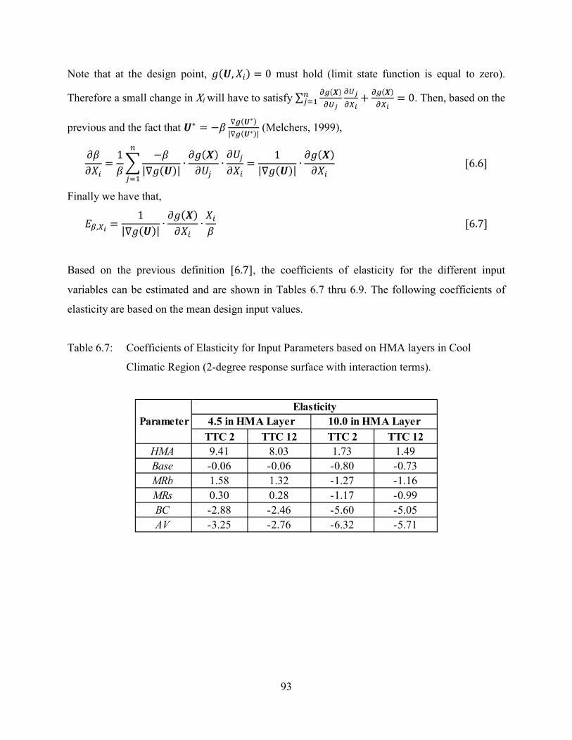
93

Note that at the design point, ( , ) = 0 must hold (limit state function is equal to zero).

Therefore a small change in Xi will have to satisfy ∑ ( ) + ( ) = 0. Then, based on the

previous and the fact that ∗ = − ∇ ( ∗)|∇ ( ∗)| (Melchers, 1999),

= 1 −|∇ ( )| ∙ ( ) ∙ = 1|∇ ( )| ∙ ( ) [6.6]

Finally we have that,

, = 1|∇ ( )| ∙ ( ) ∙ [6.7]

Based on the previous definition [6.7], the coefficients of elasticity for the different input

variables can be estimated and are shown in Tables 6.7 thru 6.9. The following coefficients of

elasticity are based on the mean design input values.

Table 6.7: Coefficients of Elasticity for Input Parameters based on HMA layers in Cool

Climatic Region (2-degree response surface with interaction terms).

TTC 2 TTC 12 TTC 2 TTC 12HMA 9.41 8.03 1.73 1.49Base -0.06 -0.06 -0.80 -0.73MRb 1.58 1.32 -1.27 -1.16MRs 0.30 0.28 -1.17 -0.99BC -2.88 -2.46 -5.60 -5.05AV -3.25 -2.76 -6.32 -5.71

4.5 in HMA Layer 10.0 in HMA LayerElasticity

Parameter

94

Table 6.8: Coefficients of Elasticity for Input Parameters based on HMA layers in Warm


Table 6.9: Coefficients of Elasticity for Input Parameters based on HMA layers in Hot


It can be observed from the tables that in the case of cool climatic regions and thin HMA layers,

the most important variable is the thickness of the HMA layer. The coefficient of elasticity

indicates that a 1% increase in HMA layer thickness can result in an 8.0% to 9.5% increase in the

reliability index (depending on the type of truck traffic). However, the effect of thickness of the

HMA layer decreases as the climate increases. Also significant in the case of thin HMA layers is

the effect of the volumetric properties (binder content and air void content), which opposed to

thickness of the HMA, increase as weather increases. For example, in the case of a thin

pavement section on a Hot Climatic Region, a 1% increase in air void content can be associated

with a 3.3% to 3.9% decrease in the reliability index, and a 1% increase in binder content can be

associated with a 3.0% to 3.4% decrease in the reliability index. Note that the effect on

TTC 2 TTC 12 TTC 2 TTC 12HMA 6.45 5.77 2.50 2.35Base -0.27 -0.24 -0.54 -0.52MRb 1.24 1.09 -0.89 -0.86MRs 0.26 0.24 -0.63 -0.56BC -2.46 -2.20 -4.19 -4.00AV -2.77 -2.48 -4.74 -4.52

ParameterElasticity


TTC 2 TTC 12 TTC 2 TTC 12HMA 4.97 5.72 4.75 4.39Base -0.53 -0.60 -0.80 -0.76MRb 1.10 1.25 -1.40 -1.32MRs -0.04 -0.03 -0.81 -0.71BC -2.95 -3.41 -6.30 -5.87AV -3.33 -3.85 -7.10 -6.61

ParameterElasticity


95

probability of failure is non-linear since = Φ(− ) as per [3.19], so the actual effect on

reliability depends on what the reliability index is for a given design.

In the case of thick pavement structures, the volumetric properties of the mix are consistently the

most important factors on the reliability of the pavement structure. Depending on the different

climatic and traffic conditions, a 1% increase in air void content can be associated with a 4.5% to

7.1% decrease in the reliability index, and a 1% increase in binder content can be associated with

a 4.0% to 6.3% decrease in the reliability index. However, the effect of thickness of the HMA

layer is still significant and for some conditions comparable to the effect of the modulus of the

base layer (although different in direction).

Additionally, it is important to note that the effect of the modulus of the base and subgrade

changes direction when comparing thin versus thick HMA layers. This indicates that the

pavement response is very different under these two conditions: in the case of thin HMA layers,

an increase in base or subgrade modulus can be associated with a reliability improvement.

However, in the case of thick HMA layers, the same increase in modulus of the base or subgrade

results in a detrimental effect on the reliability of the pavement structure.

6.4. SIMULATION ANALYSIS BASED ON 2-DEGREE RESPONSE SURFACE WITH INTERACTION

TERMS

As in the previous chapter, simulation was performed as an alternate means of estimating

reliability based on the 2-degree limit state function defined in [6.3] (∙) .

As before, simulation was performed using the Crude Monte Carlo and Latin Hypercube based

on a sample size of 10,000 runs and 10 repetitions. Additionally, in order to further validate the

results, Crude Monte Carlo simulation was also performed increasing the sample size to

1,000,000 and performing 50 repetitions.

The data assumptions used in the simulations are the same that were used for the SORM

analysis. The simulation results are shown in Tables 6.10 thru 6.12. The tables also show the

SORM results for comparison.

96


Region(2-degree response surface with interaction terms).




(2-degree response surface with interaction terms).

The tables show the reliability estimates based on simulation using the (∙) limit state

function are consistent with the SORM estimates and amongst the different simulation

techniques that were used.



85.45% 0.38% 88.49% 0.27% 96.33% 0.22% 97.60% 0.23%


85.46% 0.24% 88.70% 0.15% 96.53% 0.14% 97.65% 0.10%

Monte Carlo (N=1,000,000 - R=50)

85.51% 0.03% 88.64% 0.03% 96.46% 0.02% 97.66% 0.01%

SORM 85.60% - 88.71% - 96.61% - 97.76% -

Method




91.40% 0.25% 93.13% 0.16% 97.55% 0.20% 97.99% 0.20%


91.46% 0.13% 93.21% 0.14% 97.65% 0.16% 98.02% 0.15%

Monte Carlo (N=1,000,000 - R=50)

91.40% 0.03% 93.19% 0.03% 97.64% 0.01% 98.03% 0.01%

SORM 91.47% - 93.24% - 97.72% - 98.10% -

Method




93.52% 0.24% 91.13% 0.25% 91.65% 0.38% 92.84% 0.28%


93.37% 0.20% 91.06% 0.15% 91.61% 0.23% 92.94% 0.13%

Monte Carlo (N=1,000,000 - R=50)

93.42% 0.03% 91.05% 0.03% 91.61% 0.03% 92.93% 0.02%

SORM 93.51% - 91.18% - 91.81% - 93.11% -

Method


97

As was the case with the 1-degree limit state function, for a fixed sampling number (10,000) and

number of repetitions (10) the Crude Monte Carlo method exhibits higher variation in the

estimates (on average the standard error based on Latin Hypercube is approximately 65% of that

obtained using Crude Monte Carlo). Therefore, the Latin Hypercube simulations converge at a

faster rate.

Finally, if the results from the previous tables are compared to those from Section 5.5, it can be

observed that the differences in the reliability estimates using a 1-degree limit state function and

a 2-degree limit state function with interaction terms are typically less than 1% (although the

reliability estimates from the 2-degree limit state function are consistently lower).

98

99

CHAPTER 7: DIRECT MEPDG SIMULATION

As per Section 3.4, the probability of failure based on simulation can be expressed as, = [7.1] where Nf corresponds to the observed number of failures in the simulation process and N

corresponds to the total number of simulation runs. Note that ≠ , where Pt is the true

probability of failure for a given population.

Because of its nature, Nf is Binomially distributed since each simulation run corresponds to a

Bernoulli trial. Then, based on the definition of the Binomial distribution the expected value and

variance of Nf can be expressed as (Casella and Berger, 2002), = ∙ [7.2] = ∙ ∙ (1 − ) [7.3]

So, from [7.1], [7.2], and [7.3], the expected value and standard deviation of Pf can be estimated

as follows, = [7.4] = ∙ (1 − ) [7.5]

Based on the previous information, it is possible to establish confidence bounds in the estimate

of Pf. Assume Pf is Normally distributed with mean and standard deviation as per [7.4] and [7.5] (the assumption is correct when the number of simulation repetition increases because of the

Central Limit Theorem, CLT). Then, the 2-sided confidence bound on Pf is given by, − / ≤ − ≤ / = 1 − [7.6] − / ∙ ≤ ≤ + / ∙ = 1 − [7.7] where Z corresponds to the 2-tailed z-value and 1 – α corresponds to the level of confidence.

100

7.1. ERROR ASSOCIATED WITH THE SIMULATION

The confidence interval in [7.6] can be easily modified to become the confidence interval in the

error associated with Pf , = , as follows, − / ∙ ≤ − ≤ / ∙ = 1 − [7.8]

− / ∙ ∙ (1 − ) ≤ − ≤ / ∙ ∙ (1 − ) = 1 − [7.9]

− / ∙ (1 − )∙ ≤ − ≤ / ∙ (1 − )∙ = 1 − [7.10]

− / ∙ (1 − )∙ ≤ ≤ / ∙ (1 − )∙ = 1 − [7.11] Then for a 95% level of confidence we have that,

−1.96 ∙ (1 − )∙ ≤ ≤ 1.96 ∙ (1 − )∙ = 0.95 [7.12] Note that, on average, for all analyzed scenarios in Chapters 5 and 6, the probability of failure of

the pavement structure was determined to be between 2% and 16%, depending on the climatic

conditions surrounding the pavement structure, the thickness of the HMA layer, and the assumed

traffic loading distributions.

Assuming an acceptable error in the reliability estimate of approximately ± 3% (for a level of

reliability in the order of 90%), then, based on [7.12] the number of simulations required based

on the probability of failure would be less than 385. This allows for the possibility of using the

MEPDG itself to estimate the probability of failure of the pavement structure by means of “true”

simulation (using the implicit limit state function of the MEPDG and not relying on

approximations provided by response surfaces.).

7.2. DIRECT SIMULATION USING THE MEPDG

In order to verify the reliability results based on second moment and simulation techniques using

1-degree and 2-degree response surfaces with interaction terms, direct simulation using the

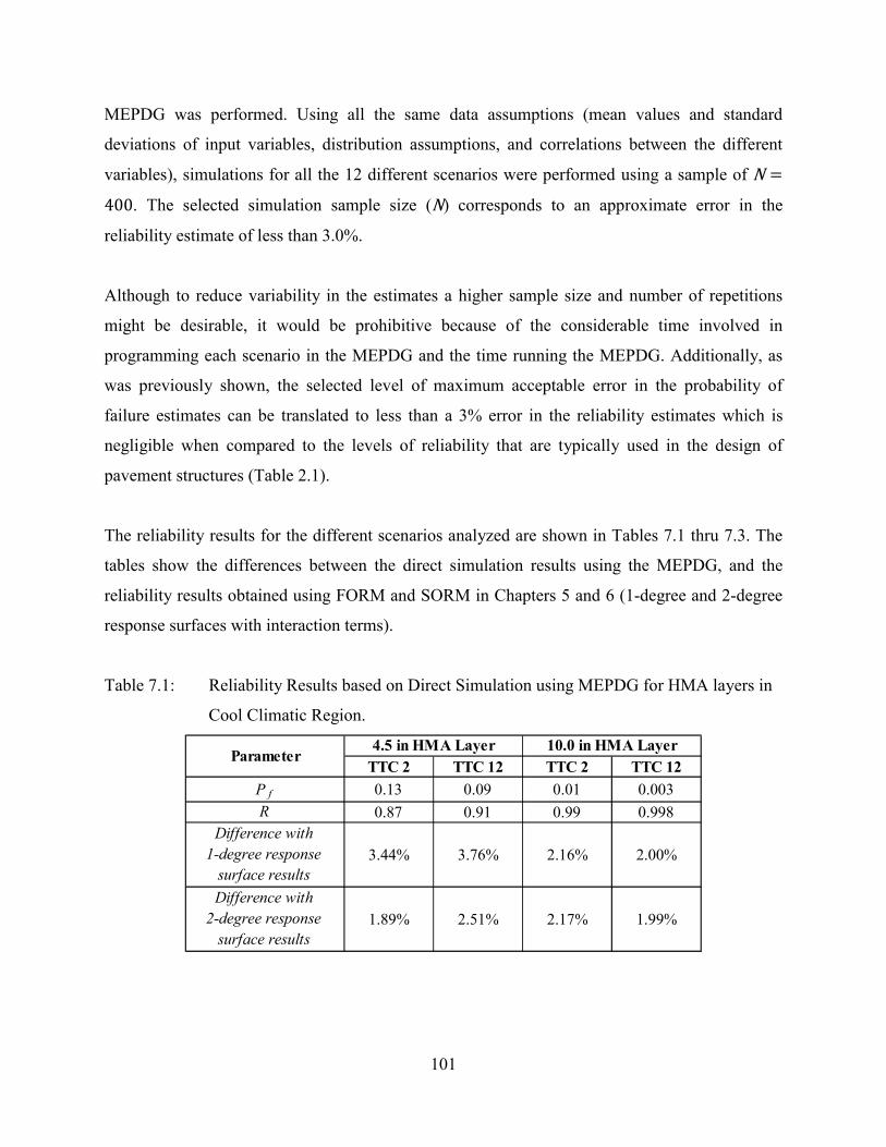
101

MEPDG was performed. Using all the same data assumptions (mean values and standard

deviations of input variables, distribution assumptions, and correlations between the different

variables), simulations for all the 12 different scenarios were performed using a sample of N = 400. The selected simulation sample size (N) corresponds to an approximate error in the

reliability estimate of less than 3.0%.

Although to reduce variability in the estimates a higher sample size and number of repetitions

might be desirable, it would be prohibitive because of the considerable time involved in

programming each scenario in the MEPDG and the time running the MEPDG. Additionally, as

was previously shown, the selected level of maximum acceptable error in the probability of

failure estimates can be translated to less than a 3% error in the reliability estimates which is

negligible when compared to the levels of reliability that are typically used in the design of

pavement structures (Table 2.1).

The reliability results for the different scenarios analyzed are shown in Tables 7.1 thru 7.3. The

tables show the differences between the direct simulation results using the MEPDG, and the

reliability results obtained using FORM and SORM in Chapters 5 and 6 (1-degree and 2-degree

response surfaces with interaction terms).

Table 7.1: Reliability Results based on Direct Simulation using MEPDG for HMA layers in

Cool Climatic Region.


0.13 0.09 0.01 0.003

0.87 0.91 0.99 0.998

3.44% 3.76% 2.16% 2.00%

1.89% 2.51% 2.17% 1.99%

Difference with 1-degree response

surface results


surface results


P f

R

102


Warm Climatic Region.


Hot Climatic Region.

Based on the direct simulation results, it can be observed that the estimates obtained using the 1-

degree and 2-degree response surfaces with interaction terms are accurate since the differences

are on average 2.64% based on the estimates from the 1-degree response surface and 2.09%

based on the estimates from the 2-degree response surface. It can be noted that the higher

differences occur in the case of thin HMA pavement layers (4.5 in) under TTC12 truck traffic

(higher percentage of single unit trucks), followed by the TTC2 truck traffic (single trailer

trucks) under the same thickness condition.


0.06 0.03 0.02 0.03

0.94 0.97 0.99 0.98

3.75% 4.16% 0.94% 0.49%

2.95% 3.62% 0.79% 0.62%

10.0 in HMA Layer

P f

RDifference with

1-degree response surface results


surface results

Parameter4.5 in HMA Layer


0.04 0.05 0.07 0.06

0.96 0.95 0.93 0.94

3.08% 4.48% 1.60% 1.74%

2.59% 3.76% 1.01% 1.21%


surface results


surface results


P f

R

103

The difference in the estimates with the pavement structures with thick HMA layers (10.0 in) are

considerably lower for most of the cases, as compared the thin HMA layer scenarios. Finally, it

is important to note that the differences between the reliability estimates using the MEPDG

directly and the estimates from SORM are consistently smaller than those from FORM. This

indicates that using the 2-degree response surface with interaction terms and using SORM to

correct for curvature improves the reliability estimates, especially in the cases when there is

higher variability associated with the results (thin HMA layer).

7.3. CHANGE IN RELIABILITY WITH TIME

Rutting in the different layers of the pavement structure is a time dependent process. It is also

highly dependent on the seasonal climatic factors. Consequently, it is interesting to evaluate how

the reliability of a pavement structure changes with time. Evaluating the change in reliability

with time allows for better management of the pavement infrastructure since time to failure or to

reach a given level of deterioration can be determined more accurately.

The data from the simulations was used to assess how reliability, or the probability of failure,

changes with time. Figure 7.1 shows how the probability of failure changes with time for the

different analysis scenarios.

Figure 7.1

From the figure it can be observe

probabilities of failure for the diffe

always the rule. Based on the diffe

earlier age in thin pavement struc

progresses, the deterioration rate (

pavements under warm and hot clim

more sensitive to rutting under higher

An interesting observation is that pro

thin HMA layers under cool or warm

the case of pavement structures under

Additional observation to Figure 7

approximately at an exponential rate

at year 15, the probability of failure w

104

: Change in reliability with time.

ed that, in general, the relative order or ranki

ferent analysis scenarios remains. Nonetheless, t

erent scenarios, it appears that failures are obse

ctures under cool climatic conditions. Howeve

number of failures observed) grows at a faste

matic conditions. This is expected because HMA

r temperatures.

obabilities of failure are higher for pavement struc

m climatic conditions. However, the trend is the o

r hot climatic conditions.

7.1 seems to show that the probabilities of fai

. What this means is that given a fixed probability

will have increased by a magnitude of 4 in a 2 ye

ing of the

this is not

erved at an

er, as time

er rate for

A layers are

ctures with

opposite for

ilure grow

y of failure

ears period,

105

and will be over 20 times as large in a 5 year period. This is very valuable information to the

pavement manager since the costs of performing maintenance activities on a given road at year

15 will also grow exponentially in the following years since simple maintenance might no longer

be an option but rehabilitation might be required.

106

107

CHAPTER 8: SENSITIVITY TO RESPONSE SURFACE

Based on the results from Chapters 5 through 7, it is reasonable to conclude that the curvature of

the failure function is low. This can be observed in the relatively small differences between the

FORM and SORM results, as well as the small differences in the reliability results obtained by

means of a linear response surface and by means of direct simulation (as per Chapter 7).

Because of the degree of curvature of the failure function, it is realistic to assume that a reduction

in the experimental design initially proposed to fit the response surfaces is valid. A valuable

outcome of this analysis would be obtained if it can be shown that similar results can be achieved

by reducing the number of MEPDG runs required to fit a response surface.

In order to assess the previous statement, the following reduced factorial was used in order to fit

the MEPDG rutting response surfaces. For each analysis scenario (different truck traffic, HMA

layer thickness, and climatic combinations) the MEPDG was run a total of 64 times for all the

combinations of the following values of the selected random variables (full factorial):

• HMA Thicknesses (HMA): mean, – 1 SD. • Asphalt Binder Content (BC): mean, + 1 SD. • Air Voids (AV): mean, + 2 SD. • Base Thickness (Base): mean, – 1 SD. • Base Modulus (MRb): mean, – 1 SD. • Subgrade Modulus (MRs): mean, – 1 SD.

where SD denotes standard deviation. The previous selection of ± 1 SD and + 2 SD was based on

the assumption that moving in the given direction of the random variable more failures would be

observed, and on the results from the elasticity analysis presented in Section 6.3.

As was the case in Chapters 5 through 7, all the previous combinations of random variables were

evaluated using the MEPDG (for a 17 year design period) at the three selected climatic regions

(cool, warm, and hot), two truck traffic distributions (TTC 2 and TTC 12), and two significantly

different thickness of the HMA layer (4.5 in and 10.0 in). Based on the 64 combinations of the

reduced factorial experiment, the HMA rutting model response surfaces were developed.

108

8.1. DEVELOPMENT OF REDUCED 1-DEGREE RESPONSE SURFACES FOR RUTTING

PERFORMANCE

The reduced response surfaces , consists of a linear approximation

to the rutting as determined by the MEPDG, and can be represented in mathematically as [5.1]. The detailed parameter estimates and standard errors are presented in the following tables.






t-stat

Intercept0.405

(0.015)26.5

0.398 (0.015)

26.7-0.031 (0.005)

-6.7-0.030 (0.005)

-6.5

HMA-0.074

(1.41x10-3)-52.6

-0.073 (1.38x10-3)

-52.9-0.006

(0.17x10-3)-34.3

-0.006 (0.17x10-3)

-33.3

Base1.67x10-4

(3.03x10-4)0.6

1.83x10-4 (2.95x10-4)

0.610.20x10-4 (0.95x10-4)

10.810.13x10-4 (0.94x10-4)

10.7

MRb-1.85x10-6 (4.79x10-8)

-38.7-1.79x10-6 (4.67x10-8)

-38.31.19x10-6

(1.49x10-8)79.8

1.19x10-6 (1.49x10-8)

80.1

MRs-7.63x10-6 (2.49x10-7)

-3.1-8.38x10-6 (2.43x10-7)

-3.52.05x10-6

(7.79x10-7)26.3

1.90x10-6 (7.78x10-7)

24.4

BC0.019

(1.57x10-3)11.9

0.018 (1.53x10-3)

11.90.024

(0.49x10-3)48.8

0.024 (0.49x10-3)

48.2

AV0.015

(1.46x10-3)10.3

0.015 (1.42x10-3)

10.40.019

(0.46x10-3)42.3

0.019 (0.46x10-3)

41.9

R 2

σ

Variable


0.988 0.988 0.996 0.995

0.002 0.002 0.001 0.001

109







t-stat

Intercept0.321

(0.014)22.3

0.327 (0.014)

23.10.029

(0.004)6.9

0.029 (0.004)

6.9

HMA-0.058

(1.33x10-3)-43.5

-0.057 (1.31x10-3)

-44.0-0.009

(0.15x10-3)-62.9

-0.009 (0.15x10-3)

-61.6

Base8.88x10-4

(2.85x10-4)3.1

8.06x10-4 (2.80x10-4)

2.96.50x10-4

(0.85x10-4)7.7

6.54x10-4 (0.85x10-4)

7.7

MRb-1.60x10-6 (4.51x10-8)

-35.5-1.59x10-6 (4.43x10-8)

-35.91.08x10-6

(1.34x10-8)81.0

1.09x10-6 (1.35x10-8)

81.1

MRs-1.01x10-6 (2.34x10-7)

-4.3-1.13x10-6 (2.30x10-7)

-4.91.46x10-6

(6.97x10-7)21.0

1.35x10-6 (7.02x10-7)

19.3

BC0.018

(1.48x10-3)12.2

0.017 (1.45x10-3)

12.00.023

(0.44x10-3)51.5

0.022 (0.44x10-3)

50.8

AV0.015

(1.38x10-3)10.7

0.014 (1.35x10-3)

10.40.018

(0.41x10-3)45.0

0.018 (0.41x10-3)

44.3

R 2

σ

Variable


0.984 0.984 0.996 0.996

0.002 0.002 0.001 0.001





t-stat

Intercept0.218

(0.013)16.6

0.221 (0.013)

16.60.041

(0.004)9.5

0.042 (0.004)

9.6

HMA-0.041

(1.21x10-3)-33.8

-0.041 (1.23x10-3)

-33.7-0.011

(0.15x10-3)-69.7

-0.011 (0.16x10-3)

-68.9

Base12.52x10-4 (2.60x10-4)

4.812.88x10-4 (2.63x10-4)

4.97.19x10-4

(0.88x10-4)8.1

7.37x10-4 (0.89x10-4)

8.3

MRb-1.18x10-6 (4.11x10-8)

-28.9-1.20x10-6 (4.17x10-8)

-28.81.16x10-6

(1.40x10-8)83.2

1.17x10-6 (1.40x10-8)

83.5

MRs-1.74x10-6 (2.13x10-7)

-0.8-2.18x10-6 (2.17x10-7)

-1.01.30x10-6

(7.28x10-7)18.0

1.23x10-6 (7.31x10-7)

16.9

BC0.019

(1.35x10-3)14.1

0.019 (1.37x10-3)

14.00.023

(0.46x10-3)50.9

0.023 (0.46x10-3)

50.3

AV0.015

(1.25x10-3)12.2

0.016 (1.27x10-3)

12.20.019

(0.43x10-3)44.3

0.019 (0.43x10-3)

43.7

R 2

σ

Variable


0.976 0.976 0.997 0.997

0.002 0.002 0.001 0.001

110

It can be observed from Tables 8.1 thru 8.3 that most of the parameters are significant at 5

percent significance level, as was the case with the full experimental design used in Chapter 5.

The exceptions are the thickness of the base layer for predicting the rutting of a thin HMA layer

(4.5 in) on a Cold Climatic Region, and the modulus of the subgrade for the thin pavement on a

Hot Climatic Region. However, the variables were not dropped from the analyses because in all

of the models they were found to be jointly significant (with the other input variables) in the

prediction of HMA rutting.

As was the case with the full factorial experimental design response surfaces, the fit of the

response surfaces, as measured by R2, is very good and for all scenarios higher than 97%. Like

all previously fit response surfaces, it was also noted that the efficiency of the models increased

when the thickness of the HMA layer is increased from 4.5 in to 10.0 in (as measured by the

reduction in model standard error associated with the change in HMA layer pavement).

Finally, based on the previously estimated response surfaces (Tables 8.1 thru 8.3), the limit state

function for rutting of the HMA layer (in inches), using the reduced experimental design, can be

defined as follows, , ( , , , , , , )= 0.25 − , [8.1] where the limit state function depends on the 0.25 in threshold for HMA layer rutting (default

failure criterion in the MEPDG), and includes a disturbance term ( ~ [0, ]) to account for

unobserved factors affecting the rutting of the HMA layer.

8.2. FORM ANALYSIS BASED ON REDUCED 1-DEGREE RESPONSE SURFACE

As in previous chapters, FORM analysis was performed assigning the variability presented in

Table 5.1, assuming Normal distributions with means and standard deviations as per Table 5.2,

and the correlation coefficients determined in Chapter 4 to the different input parameters.

Additionally, the parameters are not presumed independent but correlated as per Section 5.1.

111

The results from FORM, using the limit state function [8.1] are shown in Tables 8.4 thru 8.6.

The tables show how do the results differ from the equivalent estimates using the full factorial

design (Chapter 5 results).

Table 8.4: Reliability Analysis based on FORM and Simulation for HMA layers in Cool

Climatic Region (1-degree reduced response surface).


0.16 0.12 0.02 0.02

0.84 0.88 0.98 0.98

0.14% 0.71% 0.98% 0.73%

HMA 0.89 0.89 0.16 0.15

Base 0.00 0.00 0.02 0.02

MRb 0.03 0.03 0.09 0.09

MRs 0.00 0.00 0.03 0.02

BC 0.04 0.04 0.34 0.34

AV 0.04 0.04 0.38 0.38

ε 0.00 0.00 0.00 0.00


P f-FORM

R FORM

Difference with Full Factorial FORM

α 2

Parameter

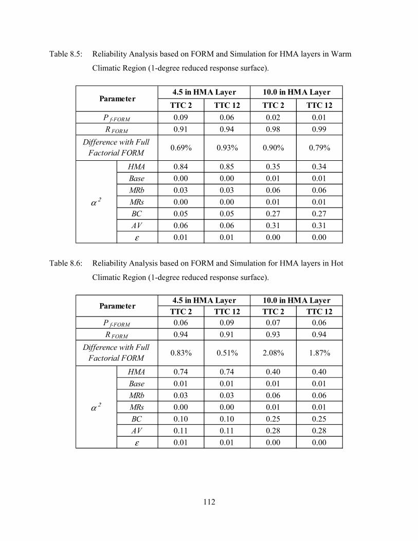
112

Table 8.5: Reliability Analysis based on FORM and Simulation for HMA layers in Warm


Table 8.6: Reliability Analysis based on FORM and Simulation for HMA layers in Hot



0.09 0.06 0.02 0.01

0.91 0.94 0.98 0.99

0.69% 0.93% 0.90% 0.79%

HMA 0.84 0.85 0.35 0.34

Base 0.00 0.00 0.01 0.01

MRb 0.03 0.03 0.06 0.06

MRs 0.00 0.00 0.01 0.01

BC 0.05 0.05 0.27 0.27

AV 0.06 0.06 0.31 0.31

ε 0.01 0.01 0.00 0.00

α 2


P f-FORM

R FORM


TTC 2 TTC 12 TTC 2 TTC 120.06 0.09 0.07 0.06

0.94 0.91 0.93 0.94

0.83% 0.51% 2.08% 1.87%

HMA 0.74 0.74 0.40 0.40

Base 0.01 0.01 0.01 0.01

MRb 0.03 0.03 0.06 0.06

MRs 0.00 0.00 0.01 0.01

BC 0.10 0.10 0.25 0.25

AV 0.11 0.11 0.28 0.28

ε 0.01 0.01 0.00 0.00


α 2


P f-FORM

R FORM

113

The results are comparable to those obtained from the response surfaces obtained from the full

factorial experiment (Chapter 5). This is the case with both the reliability estimates, as well as

with the effects measured by the squared directional cosines ( ).

It is important to highlight the small differences that were measured between the FORM

estimates using the reduced experimental design and the full factorial design. It can be observed

that the difference is on average approximately 0.9%, and is smallest in the case of thin HMA

layers in cool climatic regions (4.5 in HMA layer ) and largest in the case of thick HMA layers in

hot climatic regions (10.0 in HMA layer).

8.3. SIMULATION ANALYSIS BASED ON REDUCED 1-DEGREE RESPONSE SURFACE

As in previous chapters, simulation based on the reduced 1-degree limit state function defined in [8.1] , (∙) was also performed to compare to the FORM results. As

with previous chapters, simulation was performed using the Crude Monte Carlo and Latin

Hypercube based on a sample size of 10,000 runs and 10 repetitions, and Crude Monte Carlo

increasing the sample size to 1,000,000 and performing 50 repetitions.

The assumptions used in the simulations are the same that were used for the previous FORM

analysis. The simulation results based on the reduced response surface and how these results

compare to the simulation results based on the full factorial experiment (Chapter 5) are shown in

Tables 8.7 thru 8.9.

Table 8.7: Reliability Analysis based on simulation for HMA layers in Cool Climatic Region

(reduced 1-degree response surface).

Reliability Std. Dev. Reliability Std. Dev. Reliability Std. Dev. Reliability Std. Dev.Monte Carlo

(N=10,000 - R=10)84.35% 0.52% 88.23% 0.26% 97.68% 0.21% 98.47% 0.14%

Difference to Full Factorial Simulation


84.45% 0.20% 88.15% 0.17% 97.55% 0.17% 98.48% 0.15%


Monte Carlo (N=1,000,000 - R=50)

84.37% 0.04% 88.20% 0.03% 97.57% 0.01% 98.47% 0.01%


0.14% 0.71% 0.99% 0.73%

0.40% 0.86% 1.09% 0.68%

0.25% 0.77% 0.92% 0.75%

Method4.5 in HMA Layer 10.0 in HMA Layer


114

Table 8.8: Reliability Analysis based on simulation for HMA layers in Warm Climatic Region




As was the case with the FORM estimates, the tables show the reliability estimates based on

simulation using the , (∙) reduced limit state function are consistent with

the simulation estimates based on the full factorial experiment.

As in the previous section, very small differences were measured between the simulation

estimates using the reduced experimental design and the full factorial design. It can be observed

that the differences are on average approximately 0.95%, and were smallest in the case of thin


(N=10,000 - R=10)91.30% 0.26% 93.67% 0.29% 98.42% 0.17% 98.74% 0.05%



91.31% 0.20% 93.63% 0.18% 98.45% 0.07% 98.72% 0.10%


Monte Carlo (N=1,000,000 - R=50)

91.34% 0.02% 93.59% 0.03% 98.45% 0.01% 98.76% 0.01%


0.69% 1.03% 0.81% 0.75%

0.69% 0.93% 0.91% 0.79%

0.70% 1.02% 0.81% 0.76%




(N=10,000 - R=10)93.72% 0.19% 90.98% 0.38% 93.27% 0.26% 94.36% 0.19%



93.89% 0.15% 91.09% 0.10% 93.13% 0.22% 94.36% 0.17%


Monte Carlo (N=1,000,000 - R=50)

93.81% 0.02% 90.97% 0.02% 93.16% 0.03% 94.34% 0.02%


0.83% 0.51% 2.09% 1.87%

0.75% 0.60% 2.17% 1.77%

0.83% 0.62% 2.11% 1.89%



115

HMA layers in cool climatic regions and largest in the case of thick HMA layers in hot climatic

regions.

116

117

CHAPTER 9: CONCLUSIONS

9.1. SUMMARY AND CONCLUDING REMARKS

Proper knowledge on the variability of the different input variables used during the pavement

design process is fundamental and required information that should be available to any pavement

designer in order to produce pavement design estimates that are rational. However, as was noted

in the literature review, the variability of the many components affecting the performance of the

pavement structure during the design process are lumped together into an overall variability term

or function that was shown to produce reliability estimates different to those that would be

expected when accounting for the individual variability of the different design variables.

Towards this goal, it is essential to have pavement performance monitoring databases that

contain detailed descriptions of the materials, structure, traffic, and environment that include not

only one, but several observations or measurements of material properties and laboratory test

results and how these change with the environment. This is why the author would like to

highlight the importance of supporting and continuing with efforts such as the Long Term

Pavement Performance (LTPP) Database which has been shown to be an invaluable source of

material, structural and performance data that was used to quantify typical variances of the

different input variables that are used during pavement design. The author believes that this

information represents typical field variability and is representative of design and construction

practice in the United States, so that it can be used by pavement designers who require variability

information for their analysis or designs.

The data also allowed the author to determine what type of distributions can be used to model the

variability of the different variables in a manner that can be used with any pavement design or

analysis procedure, and is not limited to a particular dataset. Furthermore, because of the

integration of all the data into a single database, or several relational databases, it was also

possible to identify typical correlations between the different design variables. This is valuable

information because it allows for modeling of input data as correlated variables with given

distributions, as opposed to the usual assumption of independence between the different

variables. Moreover, assuming independence of the design variables will lead to inaccurate

118

material and structural behavior characterization since correlation factors of over 30 percent were

identified as part of this research project.

Then, based on accurate characterization of the variables involved in pavement design, proper

reliability analysis of pavement structures can be performed. As part of this research, a

framework to estimate reliability that can be extended to any pavement analysis or design

procedure was developed, and it was used to evaluate the reliability of pavement designs based

on the Mechanistic-Empirical Pavement Design Guide (MEPDG). The procedure requires the

use of a closed-form failure function to define failure. However, because of the mechanistic

component of the MEPDG, no closed form solution exists. Consequently, the underlying failure

function in the MEPDG has to be approximated by means of a failure response surface that can

accurately reproduce the results from the MEPDG under specific design conditions.

The failure response surfaces were initially fit based on a full factorial experimental design

where each one of the analyzed design variables (thickness of the HMA layer, air void content

and asphalt binder content of the HMA mix, thickness of the base layer, modulus of the base

layer, and modulus of the subgrade layer) was evaluated at three levels (mean value, ±1, and ±2

standard deviations from the mean, where the + or – was selected in such a way that more

failures would be observed: critical direction of the failure function). Additionally, the effect of

different climatic regions (cool, warm, and hot), different truck traffic distributions (high

percentage of single trailer trucks vs. high percentage of single unit trailers), and HMA layer

thickness (thin vs. thick) was evaluated. This resulted in 12 design scenarios for which the

MEPDG was run approximately 800 times for each. Each run consisted of analyzing the rutting

of the HMA layer in the pavement structure over a 17 year design life.

Based on the failure response surfaces for the different scenarios, reliability analysis based on

second moment techniques and simulation was performed. Both the First Order Reliability

Method (FORM) and the Second Order Reliability Method (SORM) were performed. In general,

based on the squared directional cosines ( ) of the reliability index in the standard normal

space, it was identified that the thickness of the HMA layer and the volumetric properties of the

asphalt mix (asphalt binder content and air void content) have the highest effect on rutting of the

119

HMA layer. The former is critical in the case of pavement structures with thin HMA layers, and

the latter is very important in the case of thick HMA layers. However, the conclusions based on

the directional cosines are approximate because they are based on the assumption of

independence between the analysis variables.

To further check the effect of each one of the design variables on reliability, an elasticity analysis

was performed to determine the percentage change on reliability associated with a 1% change in

each of the design variables. Similar results to the ones suggested by the directional cosines were

obtained. In the case of pavement structures with thin HMA layers, a 1% increase in HMA layer

thickness can result in up to a 9.5% increase in the reliability index. In the case of pavement

structures with thick HMA layers, a 1% increase in air void content can be associated with up to

a 7.1% decrease in the reliability index, and a 1% increase in binder content can be associated

with up to a 6.3% decrease in the reliability index.

The reliability results from SORM (which corrects for curvature of the failure function) are very

close to the FORM estimates. The difference for the different scenarios is on average 0.35%

which is negligible. This is a good indication that the failure function has a large radius of

curvature around the design point and consequently the FORM estimates are adequate. An

additional indication that the radius of curvature is large is given by the high R2 values that were

obtained by fitting the 1-degree (linear) response surfaces to the MEPDG data (over 97.5 percent

for all of the cases).

It is important to note that considerable differences were observed between the reliability

estimates using FORM and SORM, and the reliability values calculated by the MEPDG software

(confidence interval based on built-in standard deviation models used by the MEPDG). It was

found that for all the analyzed scenarios, the MEPDG reliability estimates are approximately

20% to 30% lower than the FORM estimates. This indicates that the standard error function used

by the MEPDG, [3.12], is biased and very conservative.

Additional to the FORM and SORM reliability estimates, the 1- and 2-degree failure response

surfaces were also used with simulation techniques (Monte Carlo and Latin Hypercube methods)

120

to estimate the probability of failure and reliability of the pavement structures under the 12

analysis scenarios. As expected, it was observed that for a fixed number of simulation

repetitions, the variance associated with the Latin Hypercube estimates is lower than that for the

Monte Carlo estimates. More importantly, it was found that the simulation estimates are

consistent with the FORM and SORM estimates.

All of the previous reliability estimates are based on 1- and 2-degree response surfaces because

there is no closed form solution to the MEPDG. It has been verified by means of the fit of the

response surfaces, and the differences between FORM and SORM results, that it is highly likely

that the reliability estimates are adequate. However, the only direct method to check if the results

are correct is to simulate without relying on the failure response surfaces, but to directly use the

MEPDG in a simulation analysis. However, because of the time required to run a single instance

of the MEPDG, it would be unfeasible to run millions of instances of the MEPDG to validate the

results for each of the analysis scenarios. But because of the overall magnitude in the

probabilities of failure associated with pavement structures, it was considered that 3 percent error

in the reliability estimates is still an acceptable error in the simulation of reliability. Then,

assuming the previous acceptable error, the number of simulations required for each scenario

was under 385.

Based on the previous discussion, simulations with a sample size of 400 were used to estimate

the reliability under the 12 analysis scenarios using the MEPDG directly. Based on the direct

simulation results, it was observed that the estimates obtained using the 1-degree and 2-degree

response surfaces are accurate since the differences are on average 2.64% based on the estimates

from the 1-degree response surface and 2.09% based on the estimates from the 2-degree response

surface. The small differences demonstrate that using estimated probabilities of failure based on

second moment or simulation techniques using responses surfaces is appropriate to calculate the

reliability of an MEPDG analysis or design.

Finally, it was the intention of the author for the framework described in the report to be practical

for use in routine pavement analysis performed by pavement designers. However, it is clear that

the number of instances that were required to fit a single response surface (and the time

121

associated with it) would be prohibitive. Consequently, a sensitivity analysis to the number of

levels required to fit a response surface was performed. Considering that the true rutting of the

HMA layer failure function associated with the MEPDG must have a large radius of curvature

(adequate assumption based on all previous results), it would be safe to assume that reducing the

number of MEPDG instances required to fit a failure response surface should be valid. To this

purpose, the response surfaces for each of the analysis scenarios were fit using only 2 levels for

each of the design variables (mean value and 1 or 2 standard deviations in the direction of

failure). The reduction of one level in the experimental design resulted in reducing the number of

runs required for each scenario from approximately 800 to 64. However the reliability estimates

only changed in the order of 0.9 percent. Not only is the reduction in number of runs significant,

but it will be feasible for practitioners to set the MEPDG to run 64 instances routinely using

batch mode. Furthermore, it is expected that the next version of the MEPDG, which is expected

to become available soon (AASHTO DARWin-ME), will half the run time of each instance of

the MEPDG analysis, making it even easier for a design engineer to apply the methods shown in

the report.

122

123

REFERENCES

AASHTO. (1993). AASHTO, Guide for Design of Pavement Structures 1993. American Association of State Highway and Transportation Officials. Washington, D.C.

AASHTO. (2008). Mechanistic-Empirical Pavement Design Guide. A Manual of Practice.

Interim Edition. American Association of State Highway and Transportation Officials. Washington, D.C.

Aguiar-Moya, J.P., Banerjee, A., and Prozzi, J.A. (2009). Sensitivity Analysis of the MEPDG

Using Measured Probability Distributions of Pavement Layer Thickness. Transportation Research Board 88th Annual Meeting. Washington, D.C.

Aguiar-Moya, J.P., and Prozzi, J.A. (2011). Variability in Pavement Design and its effect on the

MEPDG. Transportation Research Board 90th Annual Meeting. Washington, D.C. Alsherri, A., and George, K.P. (1988). Reliability Model for Pavement Performance. J. Transp.

Engrg. Volume 114, Issue 3, pp. 294 – 306. Anderson, T.W., and Darling, D.A. (1952). Asymptotic theory of certain "goodness-of-fit"

criteria based on stochastic processes. Annals of Mathematical Statistics 23, pp. 193 – 212.

Attoh-Okine, N.O, and Kim, W.M. (1994). Pavement Thickness Variability and Its effect on

Determination of Moduli and Remaining Life. Transportation Research Record 1449, pp. 39 – 44. Washington, D.C.

Ayres, M.J., and Witczak, M.W. (1998). AYMA – Mechanistic Probabilistic System to Evaluate

Flexible Pavement Performance. Transportation Research Record 1629, pp. 137 – 148. Washington, D.C.

Babu, G.L.S., and Srivastava, A. (2010a). Reliability Analysis of Buried Flexible Pipe-Soil

Systems. J. Pipeline Syst. Eng. Pract. Volume 1, Issue 1, pp. 33 – 41. Babu, G.L.S., and Srivastava, A. (2010b). Reliability Analysis of Buried Flexible Pipe-Soil

Systems. Manuscript accepted for publication at the Journal of Geotechnical and Geoenvironmental Engineering.

Blom, G. (1958). Statistical Estimates and Transformed Beta-variables. Wiley, New York. Breitung, K. (1984). Asymptotic Approximations for Multinormal Integrals. Journal of

Engineering Mechanics, Vol. 110, No. 3, pp. 357 – 366. Breitung, K. (1994). Asymptotic Approximations for Probability Integrals. Springer, Berlin,

Lecture Notes in Mathematics, No. 1592.

124

Brown, J.L. (1994). Reliability in Pavement Design? Who's Kidding Whom? Transportation Research Record 1449, pp. 26 – 29. Washington, D.C.

Casella, G., and Berger, R.L. (2002). Statistical Inference. Second Edition. Duxbury Advanced

Series. Pacific Grove, California. Chadbourn, B. (2002). Development of a Quick Reliability Method for Mechanistic-Empirical

Asphalt Pavement Design. Transportation Research Board 81th Annual Meeting. Washington, D.C.

Chakroborty, P., Das, A., and Pijush, G. (2010). Determining Reliability of an Asphalt Mix

Design: Case of Marshall Method. ASCE Journal of Transportation Engineering, Vol. 136, No. 1, pp. 31 – 37.

Chan, C.L., and Low, B.K. (2009). Reliability Analysis of Laterally Loaded Piles Involving

Nonlinear Soil and Pile Behavior. J. Geotech. and Geoenvir. Engrg. Volume 135, Issue 3, pp. 431 – 443.

Cizelj, L. , Mavko, B., and Riesch-Oppermann, H. (1994). Application of first and second order

reliability methods in the safety assessment of cracked steam generator tubing. Nuclear Engineering and Design 147.

Cominsky, R., Leahy, R.B., and Harrigan, E.T. (1994). Level One Mix Design: Materials

Selection, Compaction, and Conditioning. Strategic Highway Research Program Report SHRP-A-408.

D'Agostino, R.B., and Pearson, E.S. (1973). Testing for Departures from Normality. I. Fuller

Empirical Results for the Distribution of and . Biometrika, Volume 60, Issue 3, pp. 613 – 622.

D'Agostino, R.B., Balanger, A., and D'Agostino, R.B.J. (1990). A suggestion for using powerful

and informative tests of normality. American Statistician 44, pp. 316 – 321. Darter, M. I., Hudson, W. R., Brown, J. L. (1973). Statistical Variations of Flexible Pavement

Properties and their Considerations in Design. Proceedings Annual Meeting of the Association of Asphalt Pavement Technologists, Vol. 42, pp. 589 – 613.

De Bièvre, P. (1996). "Uncertainty" or "reliability"? Accreditation and Quality Assurance:

Journal for Quality, Comparability and Reliability in Chemical Measurement, Volume 1, Number 5, pp. 195.

Ebeling, C.E. (1997). An Introduction to Reliability and Maintainability Engineering. Waveland

Press, Inc. Long Grove, Illinois.

125

Elkins, G.E., Schmalzer, P., Thompson, T., and Simpson, A. (2006). Long-Term Pavement Performance Information Management System Pavement Performance Database User Guide. Federal Highway Administration Publication No. FHWA-RD-03-088 (Interim Update).

Gui, Z., Chen, J.K., Wu, Z.Y., Zhang, H., and Shi, Y.L. (2008). Reliability Analysis of Rock

Slope Involving Multiple Failure Mechanisms. GeoCongress 2008: Geosustainability and Geohazard Mitigation (GSP 178)

Hass, R., Hudson, W. R., and Zaniewski, J. (1994). Modern Pavement Management. Krieger

Publishing Company. Malabar, Florida. Hong, F., and Prozzi, J.A. (2006). Evaluation of Equipment, Methods, and Pavement Design

Implications of the AASHTO 2002 Axle Load Spectra Traffic Methodology. Texas Department of Transportation, Report No. FHWA/TX-06/0-4510-1. Austin, Texas.

Huang, Y.H. (2003). Pavement Analysis and Design, 2nd Edition. Prentice Hall, Inc. New

Jersey. Huh, J., and Haldar, A. (2001). Stochastic Finite-Element-Based Seismic Risk of Nonlinear

Structures. J. Struct. Engrg. Volume 127, Issue 3, pp. 323 – 329. Jiang, Y., Selezneva, O.I., Mladenovic, G., Aref, S., and Darter, M.I. (2003). Estimation of

Pavement Layer Thickness Variability for Reliability-Based Design. Transportation Research Record 1849, pp. 156 – 165. Washington, D.C.

Kim, H. B., and Lee, S. J. (2002). Reliability Based Design Model Applied to Mechanistic

Empirical Pavement Design. KSCE Journal of Civil Engineering, Vol. 6, No. 3, pp. 263 – 272.

Kulkarni, R.B. (1994). Rational Approach in Applying Reliability Theory to Pavement Structural

Design. Transportation Research Record 1449, pp. 13 – 17. Washington, D.C. Manuel, L (2008). Variance Reduction Methods in Simulation. Structural Reliability Notes. The

University of Texas at Austin. Austin, Texas. Melchers, R.E. (1999). Structural Reliability Analysis and Prediction, Second Edition. John

Wiley & Sons, Ltd. New York, New York. Mollon, G., Dias, D., and Soubra, A.H. (2009). Probabilistic Analysis of Circular Tunnels in

Homogeneous Soil Using Response Surface Methodology. J. Geotech. and Geoenvir. Engrg. Volume 135, Issue 9, pp. 1314 – 1325.

NCHRP. (1972). Evaluation of AASHTO Guide for Design of Pavement Structures. NCHRP

Research Report 128, Transportation Research Board, National Research Council. Washington, D.C.

126

NCHRP. (2004). Guide for Mechanistic-Empirical Design of New and Rehabilitated Pavement

Structures. NCHRP Research Report 1-37A, Transportation Research Board, National Research Council. Washington, D.C.

Lee, J.O., Yang, Y.S., and Ruy, W.S. (2002). A Comparative Study on Reliability-Index and Target-Performance-Based Probabilistic Structural Design Optimization. Computers & Structures, Volume 80, Issues 3-4, pp. 257 – 269.

Lee, S.Y., and Haldar, A. (2003). Reliability of Frame and Shear Wall Structural Systems. II:

Dynamic Loading. J. Struct. Engrg. Volume 129, Issue 2, pp. 233 – 240. Osnes, H. Variance Reduction Techniques for Monte Carlo Simulation. SINTEF Applied

Mathematics and University of Oslo. The Diffpack Preprint Series. Pendleton, O.J. (1994). Reliability in Pavement Design: Issues, Concepts, and Significance.

Transportation Research Record 1449, pp. 8 – 12. Washington, D.C. Prowell, B.D., and Brown, E.R. (2007). Superpave Mix Design: Verifying Gyration Levels in the

Ndesign Table. National Cooperative Highway Research Program NCHRP Report 573. Washington, D.C.

Prozzi, J.A., Gossain, V., and Manuel, L. (2005). Reliability of Pavement Structures using

Empirical-Mechanistic Models. Transportation Research Board 84th Annual Meeting. Washington, D.C.

Prozzi, J.A., Aguiar-Moya, J.P., Smit, A.d.F., Tahmoressi, M., and Fults, K. (2006).

Recommendations for Reducing Superpave Compaction Effort to Improve Mixture Durability and Fatigue Performance. Texas Department of Transportation, Report No. FHWA/TX-07/0-5132-1. Austin, Texas.

Prozzi, J.A., and Hong, F. (2007). Optimum Statistical Characterization of Axle Load Spectra

Based on Load-Associated Damage. International Journal of Pavement Engineering, Volume 8, Issue 4, pages 323 – 330.

Rackwitz, R., and Fiessler, B. (1978). Structural Reliability under Combined Random Load

Sequences. Computers and Structures, Vol. 9, pp. 269 – 276. Rackwitz, R. (2001). Reliability Analysis – A Review and Some Perspectives. Structural

Safety,Volume 23, Issue 4, pp. 365 – 395. Rada, G., and Witczak, M.W. (1981). Comprehensive Evaluation of Laboratory Resilient Moduli

Results for Granular Materials. Transportation Research Record 810, pp. 23 – 33. Rajashekhar, M.R., and Ellingwood, B.R. (1995). Reliability of Reinforced-Concrete Cylindrical

Shells. J. Struct. Engrg. Volume 121, Issue 2, pp. 336 – 347.

127

Read, J., and Whiteoak, D. (2003). The Shell Bitumen Handbook. Fifth Edition. Thomas Telford Publishing. London, UK.

Rogness, R.O. (1988). Reliability and Statistical Issues of the AASHTO Pavement Design

Guide. Transportation Research Record 1200, pp. 24 – 31. Washington, D.C. Royston, J.P. (1982). Algorithm AS 177: Expected Normal Order Statistics (Exact and

Approximate). Journal of the Royal Statistical Society, Series C (Applied Statistics), Volume 31, Number 2, pp. 161 – 165.

Royston, J.P. (1983). A simple test for evaluating the Shapiro-Francia W’ Test of Non-

Normality. The Statistician 32, pp. 297 – 300. Selezneva, O.I., Jiang, Y., and Mladenovic, G. (2002). Evaluation and Analysis of LTPP

Pavement Layer Thickness Data. Federal Highway Administration Report FHWA-RD-03-041.

Shapiro, S.S., and Francia, R.S. (1972). An approximate analysis of variance test for normality.

Journal of the American Statistical Association 67, pp. 215. Shapiro, S.S. and Wilk, M.B. (1965). An analysis of variance test for normality (complete

samples). Biometrika, 52, 3 and 4, pp. 591 – 611. Su, C., Luo, X., and Yun, T. (2009). Aerostatic Reliability Analysis of Long-Span Bridges.

Manuscript accepted for publication at the Journal of Bridge Engineering. Timm, D.H., Newcomb, D.E., and Galambos, T.V. (2000). Incorporation of Reliability into

Mechanistic-Empirical Pavement Design. Transportation Research Record 1730, pp. 73 –80. Washington, D.C.

Wong, F.S. (1985). Slope Reliability and Response Surface Method. J. Geotech. Engrg. Volume

111, Issue 1, pp. 32 – 53. Wooldridge, J.M. (2002). Econometric Analysis of Cross Section and Panel Data. The MIT

Press. Cambridge, Massachusets. Xu, B., and Low, B.K. (2006). Probabilistic Stability Analyses of Embankments Based on Finite-

Element Method. J. Geotech. and Geoenvir. Engrg. Volume 132, Issue 11, pp. 1444 – 1454.

Yao, T.H.J., and Wen, Y.K. (1996). Response Surface Method for Time-Variant Reliability

Analysis. J. Struct. Engrg. Volume 122, Issue 2, pp. 193 – 201. Zhang, Z., and Damnjanović, I. (2006). Applying Method of Moments to Model Reliability of

Pavements Infrastructure. J. Transp. Engrg. Volume 132, Issue 5, pp. 416 – 424.

128

Zhao, Y.G., and Ono, T. (1998). System Reliability Evaluation of Ductile Frame Structures. J. Struct. Engrg. Volume 124, Issue 6, pp. 678 – 685.

Zhao, Y.G., and Ono, T. (1999a). New Approximations for SORM: Part 1. J. Engrg. Mech.

Volume 125, Issue 1, pp. 79 – 85. Zhao, Y.G., and Ono, T. (1999b). New Approximations for SORM: Part 2. J. Engrg. Mech.

Volume 125, Issue 1, pp. 86 – 93. Zhao, Y.G., and Ono, T. (1999c). A General Procedure for First/Second-Order Reliability

Method (FORM/SORM). Structural Safety. Volume 21, Issue 2, pp. 95 – 112. Zhao, Y.G., Ono, T., and Breitung, K. (1999). New Approximations for SORM: Part 2. J. Engrg.

Mech. Volume 128, Issue 1, pp. 130 – 132.

129

APPENDIX 1: Normality Goodness-of-Fit Tests

The current Appendix shows the estimation procedure for the goodness-of-fit tests that were

used for assessing the hypothesis that a given variable follows a normal distribution.

A1.1. SKEWNESS-KURTOSIS TEST

The Skewness – Kurtosis consists of estimating individual tests for the skewness and

kurtosis ( ) statistics and then combining them into a single normality test.

A1.1.1. Skewness

For a normal distribution = 0. Then the skewness statistics can be used for testing normality

of the sample data under the following test of hypothesis: H0 – = 0 vs., H1 – ≠ 0. The

skewness test statistic can be computed for a sample of size as follows (D’Agostino et al.,

1990),

1. Estimate from the sample data, = ∑ ( − )∑ ( − ) [ 1.1] 2. Calculate, = ( + 1)( + 3)6( − 2) / [ 1.2] = 3( + 27 − 70)( + 1)( + 3)( − 2)( + 5)( + 7)( + 9) [ 1.3] = −1 + 2 − 1 / [ 1.4] = 1√ln [ 1.5] = 2( − 1) / [ 1.6]

130

3. Calculate, = ln + + 1 [ 1.7] Where ~ Normal under the null hypothesis.

A1.1.2. Kurtosis

For a normal distribution = 3. Then the kurtosis statistic can be used for testing normality of

the sample data under the following test of hypothesis: H0 – = 3 vs., H1 – ≠ 3. The

kurtosis test statistic can be computed as follows (D’Agostino et al., 1990),

1. Estimate from the sample data,

= ∑ ( − )∑ ( − ) − 3 [ 1.8] 2. Calculate the mean and variance of , ( ) = 3( − 1)+ 1 [ 1.9] ( ) = 24 ( − 2)( − 3)( + 1) ( + 3)( + 5) [ 1.10] 3. Calculate the standardized version of , = − ( )( ) [ 1.11] 4. Calculate the third standard moment of , ( ) = 6( − 5 + 2)( + 7)( + 9) 6( + 3)( + 5)( − 2)( − 3) [ 1.12]

5. Calculate, = 6 + 8( ) 2( ) + 1 + 4( ) [ 1.13]

131

6. Calculate,

( ) = 1 − − /

( ) [ 1.14] where ( ) ~ Normal under the null hypothesis.

A1.1.3. Skewness and Kurtosis Combined Statistic

As suggested by D’Agostino and Pearson (1973) a test of normality that combines both and

is the following, = + ( ) [ 1.15]

where the statistic has approximately a (chi-squared) distribution with 2 degrees of

freedom, when the population is normally distributed.

A1.2. SHAPIRO-FRANCIA TEST

Let ( , , … , ) be the ordered sample from the random population to be tested for normality

( ) < ( ) < ⋯ < ( ) , and let denote the vector of expected values of standard normal

order statistics. Then, based on (Shapiro and Francia, 1972) an analysis of variance test for

normality is given by,

′ = ∑ ( )∑ ∙ ∑ ( ) − [ 1.16]

The distribution of is not normal, but Royston (1983) showed that the transformed variable = (1 − ) − 1 / (where is a function of sample size, n) is approximately normal.

Based on simulation, Royston (1983) showed that, = −0.048157 + 0.0197196 − 0.0119065 [ 1.17] where = log ( ) − 5. Then the mean and standard deviation of were obtained based on

smoothed and are equal to,

132

= − exp(1.693067 + 0.144167 − 0.0184928 + 0.031074485 + ⋯+ 0.0055717663 ) [ 1.18] = − exp(0.510725 − 0.1160364 − 0.0067021 + 0.054465944 + ⋯+ 0.0087397329 ) [ 1.19] Then, the Shapira-Francia test can be defined as follows, = − [ 1.20]

where the statistic follows a (0,1) distribution, when the population is normally distributed.

Note that estimating the vector of expected values of standard normal order statistics ( ) in a

sample is size requires solving the following integral (Royston, 1982),

( ) = !( − 1)! ( − )! 1 − Φ( ) Φ( ) ( ) [ 1.21] where ( ) = √ exp − and Φ( ) = ( ) . Otherwise, an approximation to

suggested by Blom (1958) is the following,

= Φ −+ [ 1.22]

Documents

SWUTC/11/161025-1 DEVELOPMENT OF RELIABLE PAVEMENT …