SWReGAP

14

CHAPTER 2

LAND COVER CLASSIFICATION AND MAPPING

John H. Lowry, Jr., R. Douglas Ramsey, Kathryn A. Thomas, Donald Schrupp, William Kepner, Todd Sajwaj, Jessica Kirby, Eric Waller, Scott Schrader, Sarah Falzarano, Lisa

Langs Stoner, Gerald Manis, Cynthia Wallace, Keith Schulz, Patrick Comer, Keith Pohs, Wendy Rieth, Cristian Velasquez,, Brett Wolk, Kenneth G. Boykin, Lee O’Brien, Julie

Prior-Magee, David Bradford, and Bruce C. Thompson.

Recommended Citation: Lowry, J. H, Jr., R. D. Ramsey, K. A. Thomas, D. Schrupp, W. Kepner, T. Sajwaj, J. Kirby, E. Waller, S.

Schrader, S. Falzarano, L. Langs Stoner, G. Manis, C. Wallace, K. Schulz, P. Comer, K. Pohs, W. Rieth, C. Velasquez, B. Wolk, K.G., Boykin, L. O’Brien, J. Prior-Magee, D. Bradford and B. Thompson. 2007. Land cover classification and mapping. Chapter 2 in J.S. Prior-Magee, et al., eds. Southwest Regional Gap Analysis Final Report. U.S. Geological Survey, Gap Analysis Program, Moscow, ID.

Corresponding authors: J. Lowry is to be contacted at jlowry@gis.usu.edu, Tel. 435-797-0653, and R. D. Ramsey is to be contacted at dougr@gis.usu.edu, Tel. 435-797-3783.

SWReGAP

15

INTRODUCTION In its "coarse filter" approach to conservation biology (Jenkins 1985, Noss 1987) gap analysis relies on maps of dominant land cover as the most fundamental spatial component of the analysis for terrestrial environments (Scott et al. 1993). For the purposes of GAP, most of the land cover of interest can be characterized as natural or semi-natural vegetation defined by the dominant plant species. Vegetation patterns are an integrated reflection of physical and chemical factors that shape the environment of a given land area (Whittaker 1965). Often vegetation patterns are determinants for overall biological diversity patterns (Franklin 1993, Levin 1981, Noss 1990) which can be used to delineate habitat types in conservation evaluations (Specht 1975, Austin 1991). As such, dominant vegetation types need to be recognized over their entire range of distribution (Bourgeron et al. 1994) for beta-scale analysis (sensu Whittaker 1960, 1977). Various methods may be used to map vegetation patterns on the landscape, the appropriate method depending on the scale and scope of the project. Projects focusing on smaller regions, such as national parks, may rely on aerial photo interpretation (USGS-NPS 1994). Mapping vegetation over larger regions has commonly been done using digital imagery obtained from satellites, and may be referred to as land cover mapping (Lins and Kleckner 1996). Generally, land cover mapping is done by segmenting the landscape into areas of relative homogeneity that correspond to land cover classes from an adopted or developed land cover legend. Technical methods to partition the landscape using digital imagery-based methods vary. Unsupervised approaches involve computer-assisted delineation of homogeneity in the imagery and ancillary data, followed by the analyst assigning land cover labels to the homogenous clusters of pixels (Jensen 2005). Supervised approaches utilize representative samples of each land cover class to partition the imagery and ancillary data into clusters of pixels representing each land cover class. Supervised clustering algorithms assign membership of each pixel to a land cover class based on some rule of highest likelihood (Jensen 2005). Supervised-unsupervised hybrid approaches are common and often offer advantages over both approaches (Lillesand and Kieffer 2000). It is important to point out that a land cover map is never considered a perfect representation of the landscape. Improvements to land cover maps can, and should be made as additional “ground truth” information about actual land cover components and spatial patterns is acquired through time. These improvements should be based on independent assessments of the map’s quality (Stoms 1994). This chapter is divided into three main sections. The first section discusses land cover map development. It begins by providing background information on the regional division of labor and the regional land cover legend. It then focuses on our land cover mapping methods, including a description of data sources, the land cover modeling approach, and the general flow of the mapping process. It concludes with a description

SWReGAP

16

of the resulting land cover map product. The second section describes the process of validating the land cover product. Background information on our approach is presented along with descriptions of the methods and results of the land cover product validation. The final section provides a discussion of the land cover mapping experience in general. In this section we discuss some of the “lessons learned” from the regional mapping effort with hopes that future mapping efforts of this nature will benefit from our experience.

METHODS Land Cover Map Development

Background

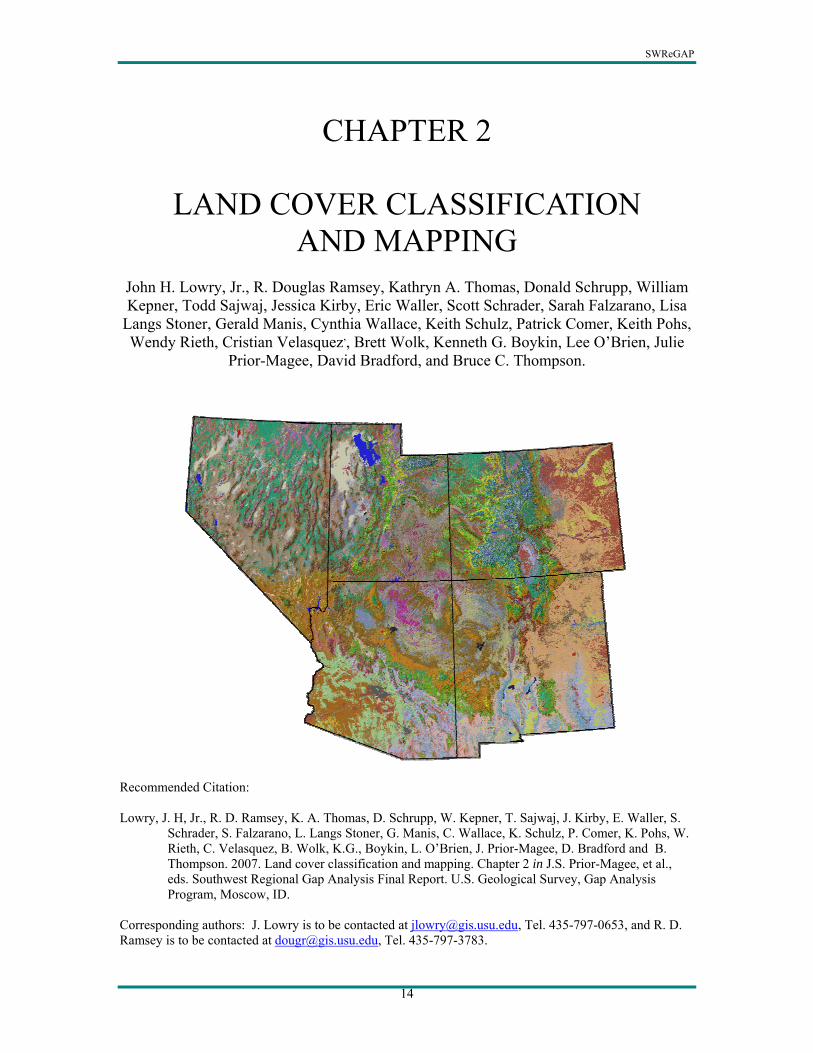
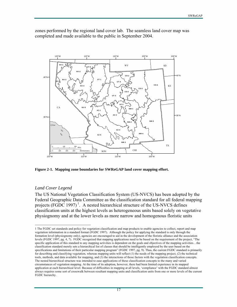
Division of Regional Responsibilities The use of “spectro-physiographic” mapping areas has proven useful for satellite-based land cover mapping by maximizing spectral differentiation between areas with relatively uniform ecological characteristics (Bauer et al. 1994, Homer et al. 1997, Lillesand 1996, Reese et al. 2002). Dividing the 1.4 million square kilometer region into spectro-physiographic “mapping zones” provided working units distributed among the five collaborating states. With the diversity of biogeographic divisions across the region, we recognized the importance of leveraging local knowledge of the biota in each sub-region. We consequently determined that a geographical approach, assigning state teams to work in their local landscapes was the most appropriate means for distributing regional mapping responsibilities. Overall project tracking and management was conducted by the regional land cover lab at Utah State University. Ecoregions defined by Bailey et al. (1994) and Omernik (1987) provided a starting point for determining the project mapping zone boundaries. These boundaries were refined by screen digitizing at a scale of approximately 1:500,000 using a regional mosaic of Landsat TM imagery resampled to 90 meters. Initial efforts yielded 73 mapping zones for the region. Through a process of iterative and collaborative steps involving all land cover mapping teams and NatureServe, the final number of mapping zones was reduced to 25 (Figure 2-1). A more detailed explanation of mapping zone development is found in Manis et al. (2000). Each state was responsible for between four and six mapping zones roughly corresponding to state jurisdictional boundaries. Initial field data collection protocols were established at a workshop in Las Vegas, Nevada in the spring of 2001. Field data collection occurred during 2002 and 2003. Land cover workshops dedicated to ensuring regionally consistent mapping methods were conducted during the winters of 2002 and 2003. Yearly meetings and monthly teleconferences involving key land cover mapping personnel from all five states and NatureServe ecologists proved invaluable throughout the collaborative mapping process. Mapping efforts were completed on a mapping zone by mapping zone basis by individual states, with the final integration of all mapping

SWReGAP

17

zones performed by the regional land cover lab. The seamless land cover map was completed and made available to the public in September 2004.

NM-5

CO-4

CO-3

AZ-5

NV-3

AZ-4

NV-4

NM-4

UT-1

AZ-2

UT-3

UT-2

NV-2

NM-3

NV-5NM-1

NM-2

AZ-1

CO-2

UT-4

AZ-3

CO-1

NV-1UT-5

NV-6

120°W

120°W

115°W

115°W 110°W

110°W

105°W

105°W

100°W

35°N35°N

40°N40°N

WY SD

SON CHI

TX

CA

0 100 200 Miles

0 100 200 300 400 Kilometers

KS

Figure 2-1. Mapping zone boundaries for SWReGAP land cover mapping effort.

Land Cover Legend The US National Vegetation Classification System (US-NVCS) has been adopted by the Federal Geographic Data Committee as the classification standard for all federal mapping projects (FGDC 1997) 1. A nested hierarchical structure of the US-NVCS defines classification units at the highest levels as heterogeneous units based solely on vegetative physiognomy and at the lower levels as more narrow and homogenous floristic units

1 The FGDC set standards and policy for vegetation classification and map products to enable agencies to collect, report and map vegetation information in a standard format (FGDC 1997). Although the policy for applying the standard is only through the formation level (physiognomy only), agencies are encouraged to aid in the development of the floristic alliance and the association levels (FGDC 1997, pg. 4, 7). FGDC recognized that mapping applications need to be based on the requirement of the project, “The specific application of this standard to any mapping activities is dependent on the goals and objectives of the mapping activities…the classification standard merely sets a hierarchical list of classes that should be intelligently employed by the user based on the specifications and limitations of their particular mapping program” (FGDC 1997, pg. 9). Thus, the current FGDC standard is primarily for describing and classifying vegetation, whereas mapping units will reflect (1) the needs of the mapping project, (2) the technical tools, methods, and data available for mapping, and (3) the interactions of those factors with the vegetation classification concepts. The nested hierarchical structure was intended to ease applications of these classification concepts to the many and varied circumstances of vegetation mapping. At the time of its adoption, however, there had been limited experience in its mapped application at each hierarchical level. Because of difficulties in mapping at all levels, ‘compliance’ with the FGDC standard almost always requires some sort of crosswalk between resultant mapping units and classification units from one or more levels of the current FGDC hierarchy.

SWReGAP

18

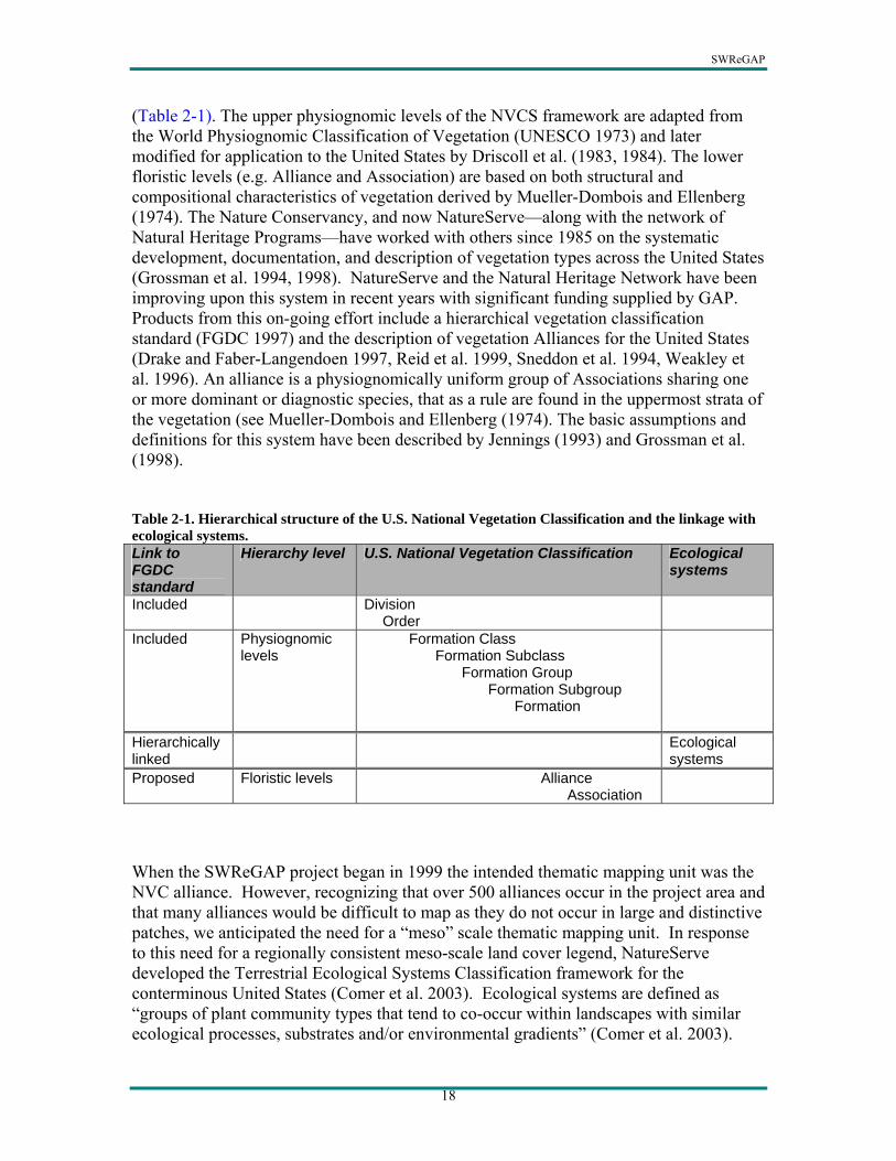
(Table 2-1). The upper physiognomic levels of the NVCS framework are adapted from the World Physiognomic Classification of Vegetation (UNESCO 1973) and later modified for application to the United States by Driscoll et al. (1983, 1984). The lower floristic levels (e.g. Alliance and Association) are based on both structural and compositional characteristics of vegetation derived by Mueller-Dombois and Ellenberg (1974). The Nature Conservancy, and now NatureServe—along with the network of Natural Heritage Programs—have worked with others since 1985 on the systematic development, documentation, and description of vegetation types across the United States (Grossman et al. 1994, 1998). NatureServe and the Natural Heritage Network have been improving upon this system in recent years with significant funding supplied by GAP. Products from this on-going effort include a hierarchical vegetation classification standard (FGDC 1997) and the description of vegetation Alliances for the United States (Drake and Faber-Langendoen 1997, Reid et al. 1999, Sneddon et al. 1994, Weakley et al. 1996). An alliance is a physiognomically uniform group of Associations sharing one or more dominant or diagnostic species, that as a rule are found in the uppermost strata of the vegetation (see Mueller-Dombois and Ellenberg (1974). The basic assumptions and definitions for this system have been described by Jennings (1993) and Grossman et al. (1998). Table 2-1. Hierarchical structure of the U.S. National Vegetation Classification and the linkage with ecological systems. Link to FGDC standard

Hierarchy level U.S. National Vegetation Classification Ecological systems

Included Division Order

Included Physiognomic levels

Formation Class Formation Subclass

Formation Group Formation Subgroup

Formation

Hierarchically linked

Ecological systems

Proposed Floristic levels Alliance Association

When the SWReGAP project began in 1999 the intended thematic mapping unit was the NVC alliance. However, recognizing that over 500 alliances occur in the project area and that many alliances would be difficult to map as they do not occur in large and distinctive patches, we anticipated the need for a “meso” scale thematic mapping unit. In response to this need for a regionally consistent meso-scale land cover legend, NatureServe developed the Terrestrial Ecological Systems Classification framework for the conterminous United States (Comer et al. 2003). Ecological systems are defined as “groups of plant community types that tend to co-occur within landscapes with similar ecological processes, substrates and/or environmental gradients” (Comer et al. 2003).

SWReGAP

19

Although distinct from the US-NVC, the vegetation component of an ecological system is described by one or more NVC alliances or associations, though this relationship is not strictly hierarchical. While the ecological system concept emphasizes existing dominant vegetation types, it also incorporates physical components such as landform position, substrates, hydrology, and climate. In this manner, ecological system descriptions are modular, having multiple diagnostic classifiers used to identify several ecological dimensions of the mapping unit (Di Gregorio and Jansen 2000). Diagnostic classifiers include environmental and biogeographic characteristics, which are incorporated in the ecological system name thus providing descriptive information about the system through a standardized naming convention. More detailed information about the Terrestrial Ecological Systems Classification for the United States is available at http://www.natureserve.org/publications/usEcologicalsystems.jsp. NatureServe Terrestrial Ecological Systems present one approach for mapping efforts to comply with Federal Geographic Data Committee standards. They are defined in terms of the base units (alliances and associations) of the US-NVC, and may be readily attributed to the upper-most levels of the FGDC hierarchy (e.g., Division, Order, Class, Subclass). We follow this approach by attributing all mapping units to NLCD land cover classes 1 and 2 (Appendix 2-3 and 2-13) which closely follow these upper FGDC levels. This approach facilitates application of these mapped data to these hierarchical levels. The initial SWReGAP target legend developed by NatureServe and the mapping teams identified approximately 110 potentially mappable ecological systems from the 140 that occur in the five-state region. Omitted ecological systems were mostly small patch (below minimum mapping unit) or peripheral to the region and lacked adequate training sites. The Terrestrial Ecological Systems Classification focuses on natural and semi-natural ecological communities. For SWReGAP, altered and disturbed land cover and land use classes were considered separately. These classes were incorporated into the SWReGAP legend using descriptions adopted from either the National Land Cover Dataset 2001 legend (e.g. Agriculture, Developed-Medium-High Intensity) (Homer et al. 2004) or were given a special “altered or disturbed” designation within the SWReGAP legend (e.g. recently burned, recently logged areas, invasive annual grassland, etc.).

Land Cover Mapping Methods

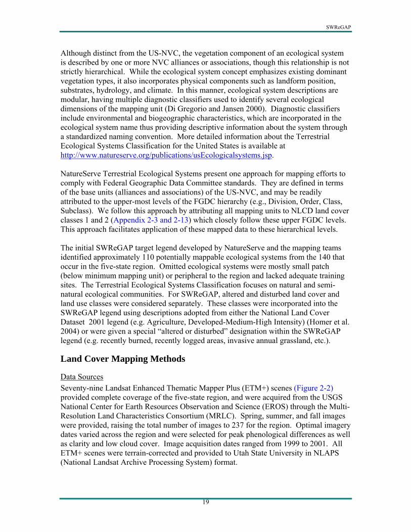
Data Sources Seventy-nine Landsat Enhanced Thematic Mapper Plus (ETM+) scenes (Figure 2-2) provided complete coverage of the five-state region, and were acquired from the USGS National Center for Earth Resources Observation and Science (EROS) through the Multi-Resolution Land Characteristics Consortium (MRLC). Spring, summer, and fall images were provided, raising the total number of images to 237 for the region. Optimal imagery dates varied across the region and were selected for peak phenological differences as well as clarity and low cloud cover. Image acquisition dates ranged from 1999 to 2001. All ETM+ scenes were terrain-corrected and provided to Utah State University in NLAPS (National Landsat Archive Processing System) format.

SWReGAP

20

3838 34383638 35383238

37383138

3338

34373837 363737373137

3937 353732373337

343637363836 36363936 3536 333631363236

4035 343537353835333535353935 3635

3235 3135

4234 4034 33343434373438343234

36344134 3934 35343134

40334233 3333 323337333833 3633 343339334133 3533

40324232 3332 3232373239324132 3832 343235323632

4332

3133

38313931 37314031 36314131 35314231

3132

34314331

4333

3331 32314431

120°W

120°W

115°W

115°W 110°W

110°W

105°W

105°W

100°W

35°N35°N

40°N40°N

WY SD

SON CHI

TX

CA

0 100 200 Miles

0 100 200 300 400 Kilometers

KS

Figure 2-2. SWReGAP area showing Landsat ETM+ scenes Our approach involved modeling image mosaics for each mapping zone (see Figure 2-1) including a 2 kilometer buffer (i.e. a 4 kilometer overlap between mapping zones). To improve image matching, image standardization for solar angle illumination, instrument calibration, and atmospheric haze (i.e. path radiance) was necessary. We determined the most practical approach was to use an image-based method as described by Chavez (1996). Standard protocol was to use a modified COST method (Chavez 1996). We found that using Chavez’ COST method over-corrected atmospheric transmittance, particularly for scenes in the arid Southwest. To address this over-correction, we used COST without TAUz (approximate atmospheric transmittance component of the COST equation). To facilitate image standardization, web-based scripts were developed to automate the process of generating corrected images on a scene-by-scene basis. 2

2 Scripts for image standardization were web-enabled making it possible for each land cover team to standardize their own images (see http://www.gis.usu.edu/docs/projects/swgap/ImageStandardization.htm). Users upload the image header file from which the script extracts the gain and bias coefficients, the solar zenith angle, and Julian date to produce an Imagine model (.gmd) file populated with extracted values for the specified correction equation. Because dark object brightness values were sometimes unavailable, or their selection was ambiguous in some mapping zones, an alternative script was available that converted brightness values to at-sensor reflectance. A single method, either the modified COST or at-sensor reflectance, was used within any given mapping zone (i.e. the standardization method was consistent within mapping zone mosaics).

SWReGAP

21

Spatial data layer preparation included both image-derived and ancillary data sets. Core image-derived data sets included individual ETM+ bands, the Normalized Difference Vegetation Index (NDVI), and brightness, greenness and wetness bands created using Landsat ETM+ coefficients from Huang et al. (2002). Ancillary data sets were derived from 30 meter digital elevation models (DEM) obtained from the USGS National Elevation Dataset. Digital elevation model-derived data sets were created for each mapping zone and included elevation, slope (in degrees), a 9-class aspect data set, and a 10-class landform data set (Manis et al. 2001). Other ancillary data sets prepared for the region, but not used, included a “stitch map” of 1:500,000 scale state geology digital maps, a soil data set (STATSGO), and 1 kilometer resolution meteorological data (DAYMET). These data sets were not used because their scale was determined to be incompatible with the core Landsat ETM+ and 30 meter DEM-derived data sets. “Ground truth” data were collected primarily through ground-based field work. Field samples were collected by traversing navigable roads in a mapping zone and opportunistically selecting plots that met criteria of appropriate size (1-hectare minimum) and composition (stand homogeneity).3 Plot data were collected using ocular estimates of biotic and abiotic land cover elements, including percent cover of dominant species by life form (i.e. trees, shrubs, grasses, and forbs) and physical data such as elevation, slope, aspect and landform. Laptop computers using ArcView® software, Landsat imagery, digital orthophoto quads, and other ancillary information were also used for navigation and plot identification whenever possible. Each plot was identified with a paired UTM coordinate using a GPS and a visually interpreted polygon representing the survey plot.4 Generally two digital photos were taken at each plot. Field data were recorded onto hardcopy field forms and subsequently entered into a database. Sufficient data were collected to assign a NVC alliance (Grossman et al. 1998) and/or ecological system (Comer et al. 2003) label to each plot. Of an approximate total of 93,000 samples obtained for the project, roughly 45,000 were collected via ground surveys during the course of the two field seasons (Appendix 2-1). In addition to the SWReGAP ground-truthed samples as described above, these data were supplemented with sample plot data obtained from other projects roughly contemporary with the time period of our imagery (1999-2001), and via visual interpretation of aerial photography, digital orthophoto quads, or other remotely sensed imagery. Samples obtained from visual interpretation of remotely sensed imagery were given only a label identifying the land cover class. Appendix 2-1 presents the distribution of samples used in the land cover modeling process.

3 The ability to traverse all navigable roads varied by state and subsequently Colorado relied heavily on obtaining sample data from existing databases and visual image interpretation. In Arizona, navigable roads were sampled using a distance criteria coupled with assessment of vegetation homogeneity. 4 Arizona collected field samples as point features (GPS x/y location) with an estimate of the radius of vegetation type, which were subsequently polygonized using an appropriately sized buffer for each sample plot.

SWReGAP

22

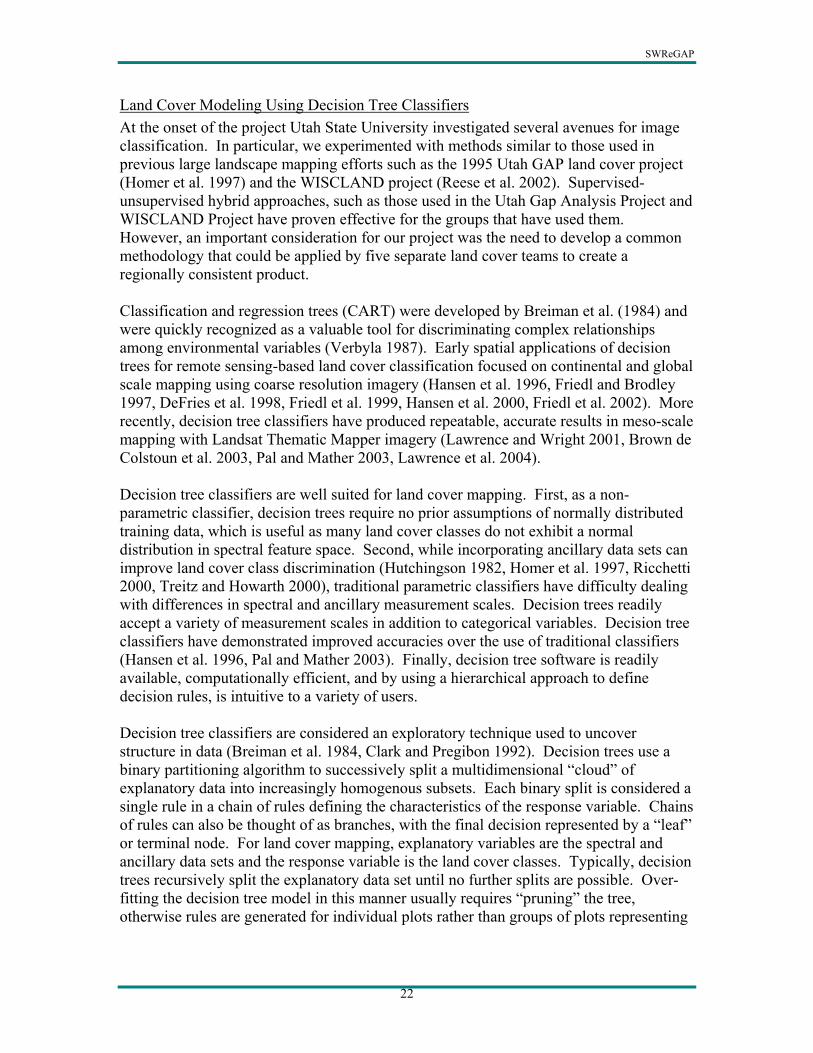
Land Cover Modeling Using Decision Tree Classifiers At the onset of the project Utah State University investigated several avenues for image classification. In particular, we experimented with methods similar to those used in previous large landscape mapping efforts such as the 1995 Utah GAP land cover project (Homer et al. 1997) and the WISCLAND project (Reese et al. 2002). Supervised-unsupervised hybrid approaches, such as those used in the Utah Gap Analysis Project and WISCLAND Project have proven effective for the groups that have used them. However, an important consideration for our project was the need to develop a common methodology that could be applied by five separate land cover teams to create a regionally consistent product. Classification and regression trees (CART) were developed by Breiman et al. (1984) and were quickly recognized as a valuable tool for discriminating complex relationships among environmental variables (Verbyla 1987). Early spatial applications of decision trees for remote sensing-based land cover classification focused on continental and global scale mapping using coarse resolution imagery (Hansen et al. 1996, Friedl and Brodley 1997, DeFries et al. 1998, Friedl et al. 1999, Hansen et al. 2000, Friedl et al. 2002). More recently, decision tree classifiers have produced repeatable, accurate results in meso-scale mapping with Landsat Thematic Mapper imagery (Lawrence and Wright 2001, Brown de Colstoun et al. 2003, Pal and Mather 2003, Lawrence et al. 2004). Decision tree classifiers are well suited for land cover mapping. First, as a non-parametric classifier, decision trees require no prior assumptions of normally distributed training data, which is useful as many land cover classes do not exhibit a normal distribution in spectral feature space. Second, while incorporating ancillary data sets can improve land cover class discrimination (Hutchingson 1982, Homer et al. 1997, Ricchetti 2000, Treitz and Howarth 2000), traditional parametric classifiers have difficulty dealing with differences in spectral and ancillary measurement scales. Decision trees readily accept a variety of measurement scales in addition to categorical variables. Decision tree classifiers have demonstrated improved accuracies over the use of traditional classifiers (Hansen et al. 1996, Pal and Mather 2003). Finally, decision tree software is readily available, computationally efficient, and by using a hierarchical approach to define decision rules, is intuitive to a variety of users. Decision tree classifiers are considered an exploratory technique used to uncover structure in data (Breiman et al. 1984, Clark and Pregibon 1992). Decision trees use a binary partitioning algorithm to successively split a multidimensional “cloud” of explanatory data into increasingly homogenous subsets. Each binary split is considered a single rule in a chain of rules defining the characteristics of the response variable. Chains of rules can also be thought of as branches, with the final decision represented by a “leaf” or terminal node. For land cover mapping, explanatory variables are the spectral and ancillary data sets and the response variable is the land cover classes. Typically, decision trees recursively split the explanatory data set until no further splits are possible. Over-fitting the decision tree model in this manner usually requires “pruning” the tree, otherwise rules are generated for individual plots rather than groups of plots representing

SWReGAP

23

land cover classes. The challenge with pruning is to establish optimal criteria so the final decision tree is neither too precise nor so general as to be meaningless. As an alternative to pruning, “ensemble techniques” can be used to produce optimal trees. Ensemble techniques involve generating multiple trees to improve model accuracy and include “bagging” and “boosting” methods. With bagging, multiple trees are generated from randomly selected subsets of the data, where the final tree is produced from a majority “vote” by all the trees. Boosting similarly subsets the data, but generates multiple trees in succession focusing on branches of the tree that are most difficult to classify (based on misclassification rates). In this sense, boosting provides a way for an optimal tree to be generated by “learning” from previous tree models. This is an important benefit considering each split in a single, non-boosted decision tree determines all subsequent splits in the branch, some of which may be sub-optimal. Boosting, rather than bagging, has been more often employed for land cover mapping applications and has produced improved accuracies relative to non-boosted approaches (Pal and Mather 2003, Brown de Colstoun 2003, Lawrence et al. 2004). A significant technical challenge with using decision trees for land cover mapping lies in the need to spatially apply the decision tree rules within a geographic information system. To successfully implement a boosted decision tree approach for such a large area among five separate teams, an effective tool for applying the decision trees in a spatially explicit context was imperative. Concurrent with our project, the USGS National Center for Earth Resources Observation and Science (EROS) began developing a land cover mapping tool capable of integrating the decision tree software See5/C5.0 (Quinlan 1993) with ERDAS Imagine. The tool, developed for the National Land cover Dataset 2001 (Homer et al. 2004) project (hereafter “NLCD mapping tool”) provided the ideal solution to our need for an efficient integration of the decision tree software within a spatially explicit modeling environment.

SWReGAP Mapping Process Land cover modeling was performed on a mapping zone by mapping zone basis with each mapping zone overlapping its adjacent mapping zone(s) with a 2 kilometer buffer (4 km overlap). The project’s primary objective was to produce the most accurate and complete map possible. To accomplish this, our mapping procedures required steps we determined made best use of all available training samples. In general, this meant two things: First, we would rely on the decision tree classifier to discriminate the bulk of the land cover classes. However, recognizing that the classifier had difficulty discriminating certain classes adequately, other methods were employed to map these classes. Natural land cover classes such as lava flows and sand dunes, which are relatively rare and/or isolated on the landscape, were typically not modeled with the decision tree, nor were

SWReGAP

24

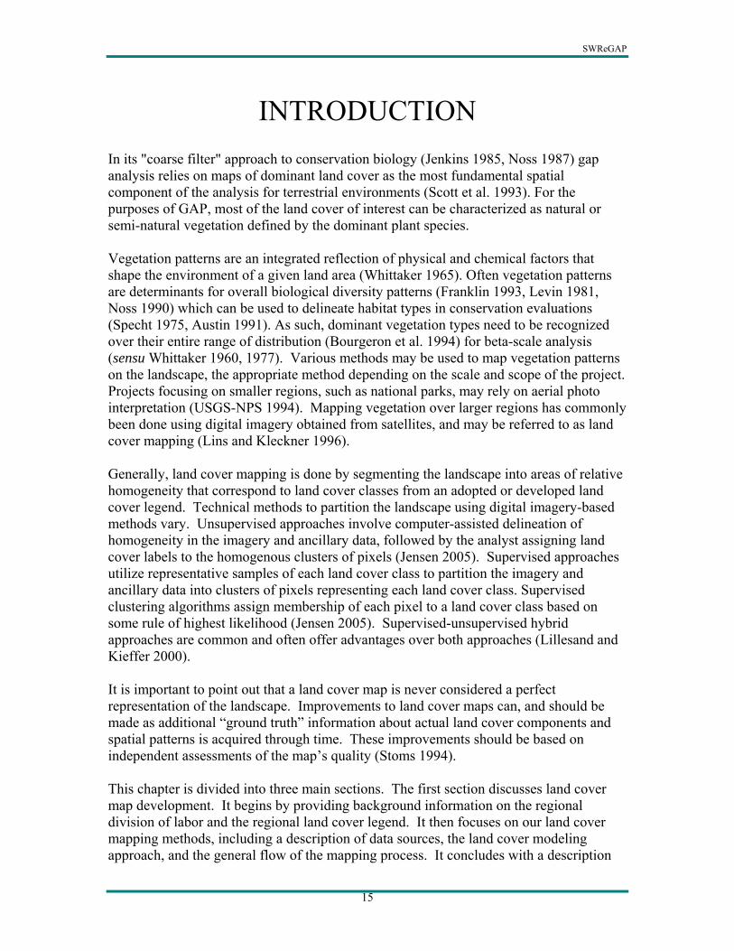
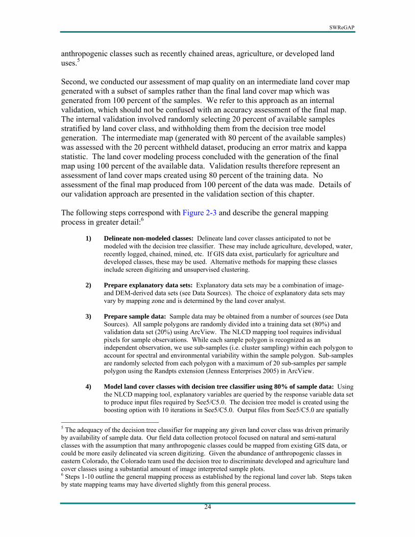
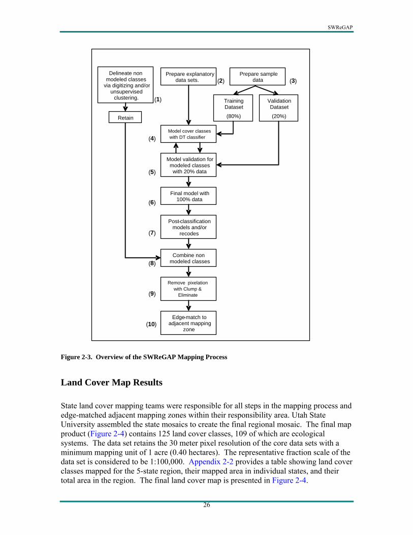
anthropogenic classes such as recently chained areas, agriculture, or developed land uses.5 Second, we conducted our assessment of map quality on an intermediate land cover map generated with a subset of samples rather than the final land cover map which was generated from 100 percent of the samples. We refer to this approach as an internal validation, which should not be confused with an accuracy assessment of the final map. The internal validation involved randomly selecting 20 percent of available samples stratified by land cover class, and withholding them from the decision tree model generation. The intermediate map (generated with 80 percent of the available samples) was assessed with the 20 percent withheld dataset, producing an error matrix and kappa statistic. The land cover modeling process concluded with the generation of the final map using 100 percent of the available data. Validation results therefore represent an assessment of land cover maps created using 80 percent of the training data. No assessment of the final map produced from 100 percent of the data was made. Details of our validation approach are presented in the validation section of this chapter. The following steps correspond with Figure 2-3 and describe the general mapping process in greater detail:6

1) Delineate non-modeled classes: Delineate land cover classes anticipated to not be

modeled with the decision tree classifier. These may include agriculture, developed, water, recently logged, chained, mined, etc. If GIS data exist, particularly for agriculture and developed classes, these may be used. Alternative methods for mapping these classes include screen digitizing and unsupervised clustering.

2) Prepare explanatory data sets: Explanatory data sets may be a combination of image-

and DEM-derived data sets (see Data Sources). The choice of explanatory data sets may vary by mapping zone and is determined by the land cover analyst.

3) Prepare sample data: Sample data may be obtained from a number of sources (see Data

Sources). All sample polygons are randomly divided into a training data set (80%) and validation data set (20%) using ArcView. The NLCD mapping tool requires individual pixels for sample observations. While each sample polygon is recognized as an independent observation, we use sub-samples (i.e. cluster sampling) within each polygon to account for spectral and environmental variability within the sample polygon. Sub-samples are randomly selected from each polygon with a maximum of 20 sub-samples per sample polygon using the Randpts extension (Jenness Enterprises 2005) in ArcView.

4) Model land cover classes with decision tree classifier using 80% of sample data: Using

the NLCD mapping tool, explanatory variables are queried by the response variable data set to produce input files required by See5/C5.0. The decision tree model is created using the boosting option with 10 iterations in See5/C5.0. Output files from See5/C5.0 are spatially

5 The adequacy of the decision tree classifier for mapping any given land cover class was driven primarily by availability of sample data. Our field data collection protocol focused on natural and semi-natural classes with the assumption that many anthropogenic classes could be mapped from existing GIS data, or could be more easily delineated via screen digitizing. Given the abundance of anthropogenic classes in eastern Colorado, the Colorado team used the decision tree to discriminate developed and agriculture land cover classes using a substantial amount of image interpreted sample plots. 6 Steps 1-10 outline the general mapping process as established by the regional land cover lab. Steps taken by state mapping teams may have diverted slightly from this general process.

SWReGAP

25

applied in Imagine using the NLCD mapping tool. Modeling is an iterative process. After model evaluation (see step 5 below) a different combination of explanatory data sets, or additional samples may be tried to improve the model. At this time the analyst decides which land cover classes are “mappable” given the availability of training data and the discriminating capabilities of the model. When model improvement reaches a point of diminishing returns, proceed to step 6.

5) Internal validation of intermediate land cover map using 20% withheld sample data:

Model validation is only for those land cover classes being modeled with the decision tree. Using the 20% withheld sample polygons, use the ArcView Kappa extension (Garrard 2003) to create an error matrix and calculate the kappa statistic (Congalton 1991). The Kappa extension intersects the validation sample polygons through the completed map. When the mode (i.e. most frequent) value of pixels in the land cover map agree with the validation polygon label, the reference site is considered correctly mapped.

6) Create final decision tree model and map using 100% of sample data: This procedure

is the same as step 4 with the exception that 100% of the sample data are used to generate the decision tree.

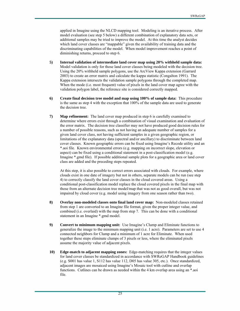
7) Map refinement: The land cover map produced in step 6 is carefully examined to

determine where errors exist through a combination of visual examination and evaluation of the error matrix. The decision tree classifier may not have produced good decision rules for a number of possible reasons, such as not having an adequate number of samples for a given land cover class, not having sufficient samples in a given geographic region, or limitations of the explanatory data (spectral and/or ancillary) to discriminate between land cover classes. Known geographic errors can be fixed using Imagine’s Recode utility and an *.aoi file. Known environmental errors (e.g. mapping on incorrect slope, elevation or aspect) can be fixed using a conditional statement in a post-classification model (e.g. Imagine *.gmd file). If possible additional sample plots for a geographic area or land cover class are added and the preceding steps repeated.

At this step, it is also possible to correct errors associated with clouds. For example, where clouds exist in one date of imagery but not in others, separate models can be run (see step 4) to correctly classify the land cover classes in the cloud covered areas. Using a conditional post-classification model replace the cloud covered pixels in the final map with those from an alternate decision tree model/map that was not as good overall, but was not impaired by cloud cover (e.g. model using imagery from one season rather than two).

8) Overlay non-modeled classes onto final land cover map: Non-modeled classes retained

from step 1 are converted to an Imagine file format, given the proper integer value, and combined (i.e. overlaid) with the map from step 7. This can be done with a conditional statement in an Imagine *.gmd model.

9) Convert to minimum mapping unit: Use Imagine’s Clump and Eliminate functions to

generalize the image to the minimum mapping unit (i.e. 1 acre). Parameters are set to use 4 connected neighbors for Clump and a minimum of 1 acre for Eliminate. When used together these steps eliminate clumps of 3 pixels or less, where the eliminated pixels assume the majority value of adjacent pixels.

10) Edge-match to adjacent mapping zones: Edge-matching requires that the integer values

for land cover classes be standardized in accordance with SWReGAP Handbook guidelines (e.g. S001 has value 1, S112 has value 112, D05 has value 305, etc.). Once standardized, adjacent images are mosaiced using Imagine’s Mosaic tool with cutline and overlap functions. Cutlines can be drawn as needed within the 4 km overlap area using an *.aoi file.

SWReGAP

26

Figure 2-3. Overview of the SWReGAP Mapping Process

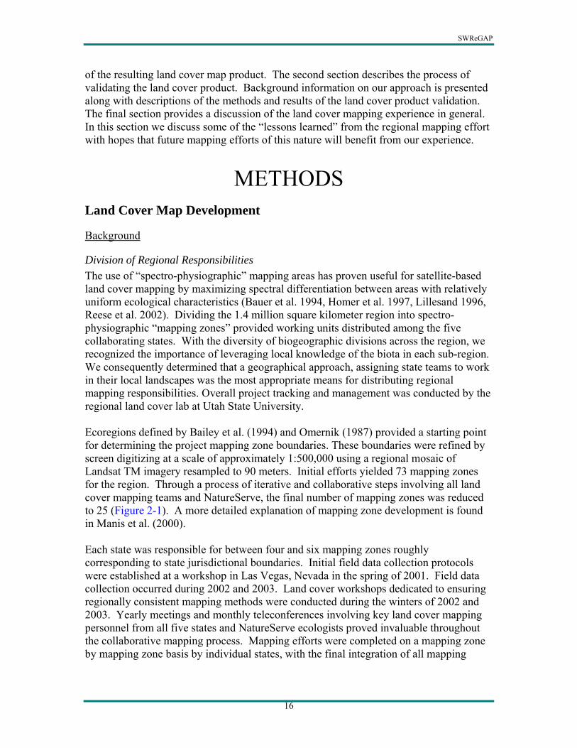
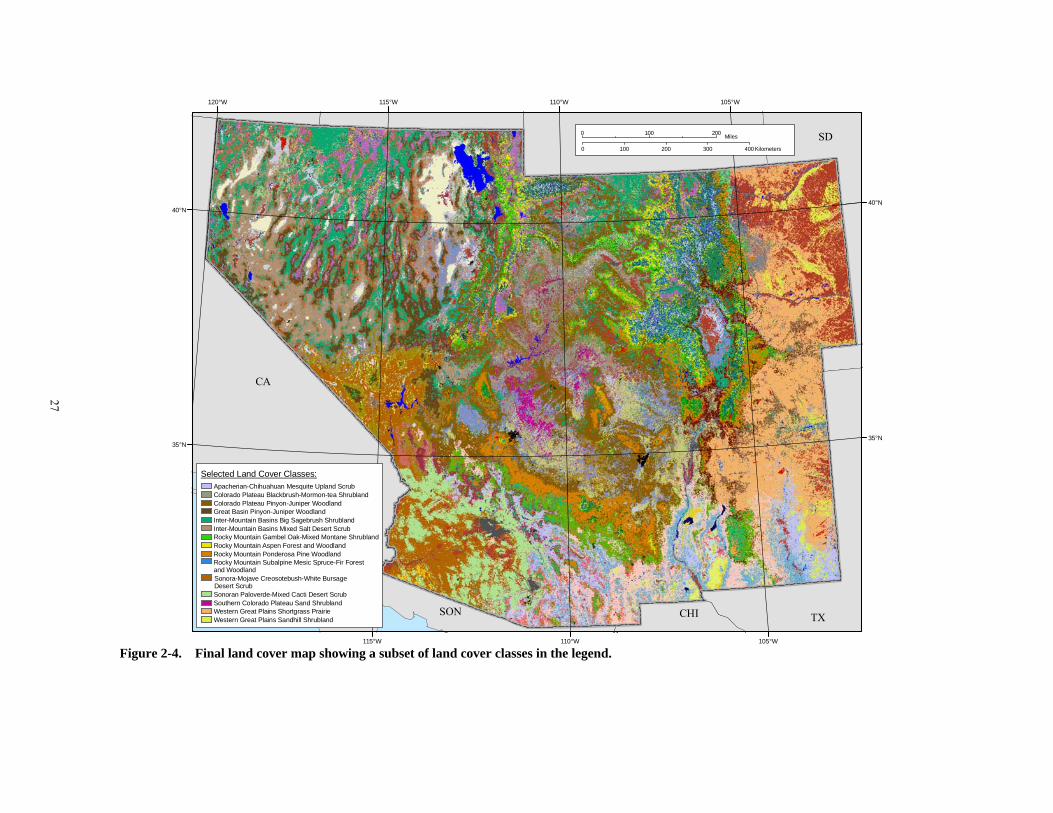
Land Cover Map Results State land cover mapping teams were responsible for all steps in the mapping process and edge-matched adjacent mapping zones within their responsibility area. Utah State University assembled the state mosaics to create the final regional mosaic. The final map product (Figure 2-4) contains 125 land cover classes, 109 of which are ecological systems. The data set retains the 30 meter pixel resolution of the core data sets with a minimum mapping unit of 1 acre (0.40 hectares). The representative fraction scale of the data set is considered to be 1:100,000. Appendix 2-2 provides a table showing land cover classes mapped for the 5-state region, their mapped area in individual states, and their total area in the region. The final land cover map is presented in Figure 2-4.

Delineate non modeled classes

via digitizing and/or unsupervised

clustering.

Prepare explanatory data sets.

Prepare sample data

Training Dataset

(80%)

Validation Dataset

(20%)Retain

Model cover classeswith DT classifier

Model validation for modeled classes

with 20% data

Final model with 100% data

Post-classification models and/or

recodes

Combine non modeled classes

Remove pixelationwith Clump &

Eliminate

Edge-match to adjacent mapping

zone

( 1 )

(2) ( 3 )

( 4 )

( 5 )

( 6 )

( 7 )

( 8 )

( 9 )

( 10 )

27

120°W

115°W

115°W 110°W

110°W

105°W

105°W

35°N35°N

40°N40°N

SD

SON CHI TX

CA

Selected Land Cover Classes:Apacherian-Chihuahuan Mesquite Upland ScrubColorado Plateau Blackbrush-Mormon-tea ShrublandColorado Plateau Pinyon-Juniper WoodlandGreat Basin Pinyon-Juniper WoodlandInter-Mountain Basins Big Sagebrush ShrublandInter-Mountain Basins Mixed Salt Desert ScrubRocky Mountain Gambel Oak-Mixed Montane ShrublandRocky Mountain Aspen Forest and WoodlandRocky Mountain Ponderosa Pine WoodlandRocky Mountain Subalpine Mesic Spruce-Fir Forest and WoodlandSonora-Mojave Creosotebush-White BursageDesert ScrubSonoran Paloverde-Mixed Cacti Desert ScrubSouthern Colorado Plateau Sand ShrublandWestern Great Plains Shortgrass PrairieWestern Great Plains Sandhill Shrubland

0 100 200 Miles

0 100 200 300 400 Kilometers

Figure 2-4. Final land cover map showing a subset of land cover classes in the legend.

SWReGAP

28

LAND COVER MAP VALIDATION

Introduction Assessing land cover map quality is an important concern for land cover mapping projects. Map quality assessment provides useful information to map users about the reliability of the map product. Various approaches to map quality assessment are recognized (Foody 2002), however, making the assessment helpful to the map user should be of primary importance (Smits et al. 1999). Typically the quality of land cover maps are assessed using a probability based sampling design (Stehman and Czaplewski 1998) with relatively large sample sizes per class (Congalton and Green 1999). These probability based approaches utilize data collected specifically for map quality assessment, and are commonly referred to as “map accuracy assessments.” We consider our approach an internal validation; “validation” in the sense that our pur-pose is to validate the quality of the map, and “internal” because we use data collected for, and used within, the modeling process (Shtatland et al. 2004). The approach may be viewed as a “split sample” or “hold out” method. This type of validation is not as accurate as a k-fold cross-validation (Goutte 1997) or as robust as an external validation (Shtatland et al. 2004). However, given the size and scope of our project, we determined itto be the most feasible approach providing a useful quantitative measure of map quality. Land Cover Map Validation Methods Quantitative validation methods were described briefly in the previous section dealing with the mapping process. Here we provide a more detailed explanation about the quantitative validation process used by SWReGAP, focusing on our use of fuzzy set analysis. We also describe our approach to performing a qualitative assessment of the map product.

Quantitative Assessment using Fuzzy Sets The Gap Analysis Handbook recommends the use of “fuzzy set” analysis as a means of providing map users additional information about the quality of the map product (Crist and Deitner 2000). Our approach to fuzzy set assessment is based on the work of Gopal and Woodcock (1994) and described by Congalton and Green (1999). Using fuzzy set analysis for map quality assessment has proven useful in various land cover mapping efforts (Falzarano and Thomas 2004, Laba et al. 2002, Woodcock and Gopal 1992, Reiners et al. 2000). The premise behind fuzzy set theory for thematic map assessment is that thematic mapping involves placing a continuum of land cover into (somewhat artificially) discrete land cover classes. This continuum suggests that there can be different magnitudes of error between/among classes. The objective of using fuzzy sets for thematic map assessment is to provide map users with information about the frequency and magnitude of map error. In other words, a reference site may have been

SWReGAP

29

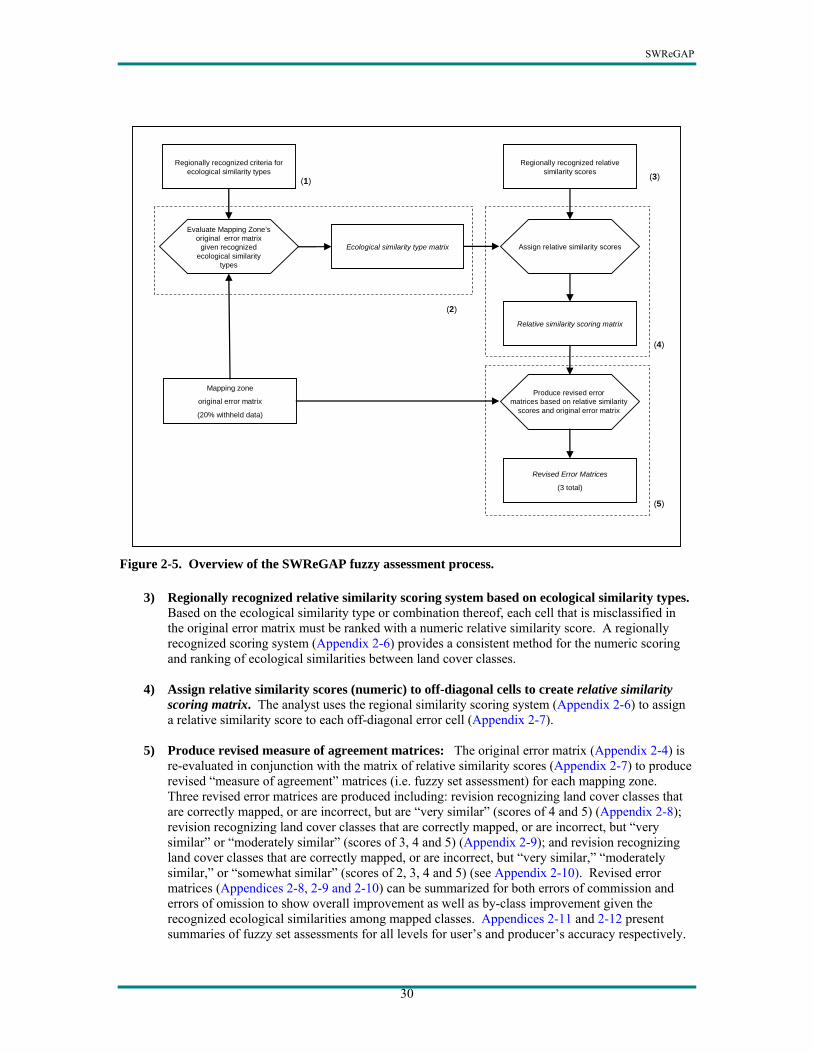
mapped incorrectly, but how incorrect was it? An answer to this question can be provided by re-evaluating the error matrix within the context of recognized similarities among land cover classes. The essence of fuzzy set assessment lies in the construction of a “linguistic measurement scale” to assign degrees of correctness to misclassification errors. Gopal and Woodcock (1994) suggest five levels of linguistic values ranging from “absolutely wrong” to “absolutely right” which experts to use when evaluating a map product relative to the reference sample plots. Determining the appropriate linguistic class, or error type, for any given reference plot is subject to the judgment of the error assessment “expert.” Establishing objective criteria for assigning the level of error, therefore, is an important component to a fuzzy set assessment. Criteria for error assignment type may be based on seriousness of the error for its intended application (Reiners et al. 2000) or on some aspect of similarity among land cover classes. Establishing criteria for defining error assessment types was particularly important for a collaborative project such as SWReGAP. For our project, each land cover team acted as the “expert” responsible for error type assignment. For the fuzzy assessment to be as regionally consistent as possible, establishing a regional framework for error assessment was critical. Our approach focused on criteria based on “ecological similarity.” Fuzzy assessments were created for each mapping zone independent of other mapping zones rather than the region as a whole. Typically, fuzzy assessments are conducted as part of an accuracy assessment after map completion. Our approach however used the error matrices produced from the internal validation (see SWReGAP Mapping Process). Figure 2-5 provides an overview of the process describing the steps in greater detail.

1) Regionally recognized criteria for ecological similarity types. Four major types of ecological similarity form the criteria from which similarity among land cover classes are recognized: physiognomic structure, dominant species, juxtaposition of ecological systems, and special substrates. Appendix 2-3 presents the regionally recognized ecological similarity types.

2) Evaluate original error matrix for ecological similarity types to create ecological similarity

type matrix. The analyst evaluates each pair of land cover classes for every off-diagonal error (misclassification) cell in the original error matrix within the context of the regionally recognized ecological similarity types. While the ecological similarity types are regionally recognized, it is incumbent upon the analyst to assign ecological similarity codes. This is done based on the analyst’s knowledge of the mapped ecological systems, and familiarity with the particular mapping zone being analyzed. An ecologist from NatureServe reviewed the state analysts’ assignment of ecological similarity codes to ensure a regionally consistent application of the ecological criteria. Appendix 2-4 provides an example of the original error matrix for UT-5 and Appendix 2-5 presents the resulting ecological similarity type matrix.

SWReGAP

30

Regionally recognized criteria for ecological similarity types

(1)

Regionally recognized relative similarity scores

Mapping zone

original error matrix

(20% withheld data)

Evaluate Mapping Zone’soriginal error matrix

given recognized ecological similarity

types

Ecological similarity type matrix Assign relative similarity scores

Relative similarity scoring matrix

Produce revised errormatrices based on relative similarity

scores and original error matrix

Revised Error Matrices

(3 total)

(3)

(2)

(4)

(5)

Figure 2-5. Overview of the SWReGAP fuzzy assessment process.

3) Regionally recognized relative similarity scoring system based on ecological similarity types. Based on the ecological similarity type or combination thereof, each cell that is misclassified in the original error matrix must be ranked with a numeric relative similarity score. A regionally recognized scoring system (Appendix 2-6) provides a consistent method for the numeric scoring and ranking of ecological similarities between land cover classes.

4) Assign relative similarity scores (numeric) to off-diagonal cells to create relative similarity

scoring matrix. The analyst uses the regional similarity scoring system (Appendix 2-6) to assign a relative similarity score to each off-diagonal error cell (Appendix 2-7).

5) Produce revised measure of agreement matrices: The original error matrix (Appendix 2-4) is

re-evaluated in conjunction with the matrix of relative similarity scores (Appendix 2-7) to produce revised “measure of agreement” matrices (i.e. fuzzy set assessment) for each mapping zone. Three revised error matrices are produced including: revision recognizing land cover classes that are correctly mapped, or are incorrect, but are “very similar” (scores of 4 and 5) (Appendix 2-8); revision recognizing land cover classes that are correctly mapped, or are incorrect, but “very similar” or “moderately similar” (scores of 3, 4 and 5) (Appendix 2-9); and revision recognizing land cover classes that are correctly mapped, or are incorrect, but “very similar,” “moderately similar,” or “somewhat similar” (scores of 2, 3, 4 and 5) (see Appendix 2-10). Revised error matrices (Appendices 2-8, 2-9 and 2-10) can be summarized for both errors of commission and errors of omission to show overall improvement as well as by-class improvement given the recognized ecological similarities among mapped classes. Appendices 2-11 and 2-12 present summaries of fuzzy set assessments for all levels for user’s and producer’s accuracy respectively.

SWReGAP

31

Qualitative Assessment It is important to recall that some land cover classes were not modeled with the decision tree classifier but were instead incorporated into the map as a post-modeling step. In addition, for some classes, withholding 20% of the available samples resulted in very few reference samples. Because of these shortfalls with the quantitative assessment, and because we believe there is value in a qualitative summary, we provide qualitative assessment summaries for each land cover class by mapping zone. Land cover qualitative summaries are brief descriptions provided by the teams involved in the mapping process for each mapping zone. They are intended to provide a qualitative evaluation from the perspective of the land cover mapping analyst of how well the land cover class appeared to be mapped, taking into consideration the number of training and reference samples available for the cover class and the team’s knowledge or familiarity with the mapping area. Often, the summary provides a narrative interpretation of the error matrix, identifying in qualitative terms where a particular land cover class is being misclassified geographically and with which land cover classes it is being confused.

Land Cover Map Validation Results

Mapping Zone Assessments Model validation as described above was performed for each mapping zone separately. While reporting kappa statistics and presenting error matrices for all 25 mapping zones is beyond the scope of this paper, these data are available to the public at http://earth.gis.usu.edu/swgap/mapquality.html. The website provides errors of omission, errors of commission, overall percent correctly modeled, as well as the kappa statistic for each mapping zone. Since our validation approach involved withholding 20 % of available sample plots proportionally stratified across the land cover classes, few reference plots for several rare land cover classes were available for validation. Rather than exclude the rare, or non-modeled classes (e.g. anthropogenic classes) in our final product, we chose to include them without validation. In addition to these quantitative data on model validation, the website also provides the qualitative evaluations provided by each state’s land cover mapping team for every land cover class by mapping zone. The qualitative evaluations provide brief narratives summarizing perceived strengths and weaknesses of the mapped class. These evaluations are provided for all land cover classes regardless of whether they were quantitatively validated or not.

Regional Assessment To provide a regional validation by land cover class, all mapping zone error matrices were combined and summarized. Appendix 2-13 presents all 125 land cover classes sorted into 5 validation groups and organized hierarchically into NLCD land cover classes. The first validation group contains classes that were not assessed regionally

SWReGAP

32

because of limited validation plots (n < 20 for the region) or were non-natural classes and not the primary focus of our mapping effort. These 40 classes comprise approximately 9.5% of the total land area for the region, with more than half (5.5%) as agriculture. The second validation group contains land cover classes with validation results from a user’s perspective less than 30%. These three classes comprise less than 0.5% of the total land area for the region. All of the classes in this group are difficult to discriminate ecologically and spectrally (i.e. a grassland, steppe and savanna). For example, the error matrices for these classes reveal that the Chihuahuan Semi-Desert Grassland was most confused with the Apacherian-Chihuahuan Semi-Desert Grassland and Steppe class, and the Basins Big Sagebrush Steppe class was most often confused with the Basins Big Sagebrush class. The next validation group contains classes where agreement between the validation samples and the map was between 30 and 49% from a user’s perspective. These 17 classes represent approximately 9.5% of the land area. Most comprise very small portions of the region (less than 0.5%) with the exception of three classes. Two scrub/shrub classes (Apacherian-Chihuahuan Mesquite Upland Scrub, Chihuhuan Mixed Desert and Thorn Scrub) and one grassland/herbaceous class (Inter-Mountain Basins Semi-Desert Grassland) represent substantial portions of the land area, covering approximately 30,000 square kilometers each. The two desert scrub classes are confused with the Apacherian-Chihuahuan Semi-Desert Grassland and Steppe class, and with each other. The Inter-Mountain Basins Semi-Desert Grassland is mostly confused with the Intermountain Basins Semi-Desert Shrub Steppe, and the Intermountain Basins Big Sagebrush Shrubland class. The obvious trend with these poorly and very poorly mapped classes is high confusion among classes that are ecologically very similar, sparsely vegetated, or both. The largest number of mapped classes (50) comprising the greatest proportion of land area (56.5%) are presented in the next validation group. Here agreement between the validation samples and the map was between 50 and 70%. The most notable classes for relative abundance on the landscape are the Colorado Plateau Pinyon-Juniper Woodland (7% land area) and Inter-Mountain Basins Big Basin Sagebrush Shrubland (8% land area) classes, with user validation rates of 69% and 59% respectively (producer’s rates of 81% and 77%). Fifteen classes were validated with results greater than 70% agreement between the validation samples and the map. These 15 classes represent approximately 24% of the total land area. The 85 classes that were validated represent 91% of the total land area. Overall correct classification for these 85 classes was 61% (KHAT statistic = 0.60; n = 17,030). The overall figure of 61% provides a summary measurement for the region of the decision tree classifier’s performance relative to the reference samples used for validation. It is important to recognize that validation results vary by land cover class (Appendix 2-13) and by mapping zone. For example, matrix-forming land cover classes

SWReGAP

33

(i.e. “extensive and contiguous…with wide ecological tolerances typically ranging in size from 2,000 to 100,000 ha” (Comer 2003)) such as certain forests, shrublands and grasslands typically represent a larger portion of the landscape and typically had a larger number of training and validation samples. These classes typically had better validation results than small or linear patch types with relatively few training and reference samples. Land cover classes on the fringe of their geographic range in some mapping zones may be more poorly mapped than elsewhere because the size and distribution of samples (both for training and validation) was limited. Lastly, it is important to note that the validation results are based on the intermediate land cover map using the 20% withheld dataset. Since the final map was produced using the withheld samples, we assume that the final map is an improvement over the intermediate map that was validated.

SWReGAP

34

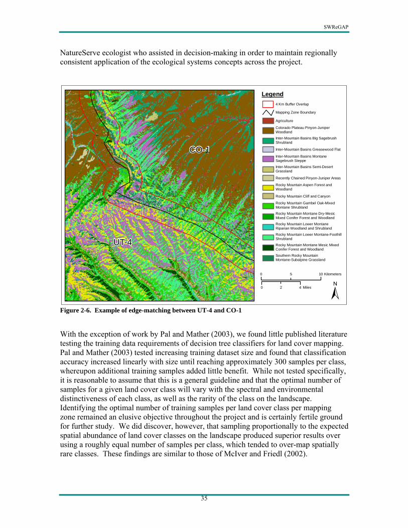
DISCUSSION Land Cover Mapping Methods A primary objective of our land cover mapping process was to develop a methodology that was repeatable and could be consistently applied by multiple land cover mapping teams. In this regard we believe the decision tree classifier method was successful. The intuitive nature of the decision tree classifier and the easy-to-use software met this objective very well. Compared to hybrid supervised-unsupervised image classification approaches used in large land cover mapping efforts (Homer et al. 1997, Reese et al. 2002, Ma et al. 2001) we found the decision tree classifier considerably more time-efficient. Whether decision tree classifiers are a more effective tool for discriminating land cover classes was not specifically researched by our project. However Hansen et al. (1996) and Pal and Mather (2003) observed a measure of superiority over traditional parametric image classification techniques. The use of spectro-physiographic mapping zones appeared to be a successful strategy for dividing the region into manageable working units and an effective means of constraining spectrally and environmentally similar land cover classes to logical geographic boundaries. Production of multi-scene mosaics for each mapping zone appeared successful as well. While image standardization did not result in seamless mosaics, satellite scene boundaries that were apparent generally were not problematic.7 This may be due to the slight effects of atmospheric attenuation in the arid southwest, and may be of greater concern in other environments. Identifying the optimal combination of predictor data sets for the decision tree classifier was a major focus in our efforts to develop a regional mapping methodology. Initially, we considered establishing a regional set of standard predictor data sets for all mapping zones in the region. Our concern was that adjacent land cover maps would not edge-match adequately if different sets of predictors were used for model development. Eventually, it was decided that each land cover analyst would choose the predictor data sets they determined worked best for a given mapping zone. As expected, the availability of multiseason imagery did improve image classification in most areas. However, use of imagery from a single season occasionally produced better results. The suite of core predictor data sets to choose from was consistent throughout the region, namely three seasons of ETM+ imagery with the analyst’s choice of image transformations, and any combination of DEM derivatives (slope, aspect, landform, etc.). Concerns about edge-matching adjacent land cover maps proved negligible in most instances. In fact, successful matching of adjacent land cover maps could indicate accurate land cover mapping since completely different models converged upon similar predictions of vegetation distribution (see Figure 2-6). Good edge-matching was also facilitated by frequent communication and coordination between the land cover mapping teams and the

7 Given highly seasonal spectral variability in Colorado, it seemed that scene boundaries needed to be accounted for. Therefore, scene boundaries were included as a predictor layer in Colorado.

SWReGAP

35

NatureServe ecologist who assisted in decision-making in order to maintain regionally consistent application of the ecological systems concepts across the project.

Legend

Southern Rocky Mountain Montane-Subalpine Grassland

Rocky Mountain Montane Mesic Mixed Conifer Forest and Woodland

Rocky Mountain Lower Montane-Foothill Shrubland

Rocky Mountain Lower Montane Riparian Woodland and Shrubland

Rocky Mountain Montane Dry-Mesic Mixed Conifer Forest and Woodland

Rocky Mountain Gambel Oak-Mixed Montane Shrubland

Rocky Mountain Cliff and Canyon

Rocky Mountain Aspen Forest and Woodland

Recently Chained Pinyon-Juniper Areas

Inter-Mountain Basins Semi-Desert Grassland

Inter-Mountain Basins Montane Sagebrush Steppe

Inter-Mountain Basins Greasewood Flat

Inter-Mountain Basins Big Sagebrush Shrubland

Colorado Plateau Pinyon-Juniper Woodland

Agriculture

4 Km Buffer Overlap

Mapping Zone Boundary

UT-4

CO-1

±0 105 Kilometers

0 42 Miles

Figure 2-6. Example of edge-matching between UT-4 and CO-1 With the exception of work by Pal and Mather (2003), we found little published literature testing the training data requirements of decision tree classifiers for land cover mapping. Pal and Mather (2003) tested increasing training dataset size and found that classification accuracy increased linearly with size until reaching approximately 300 samples per class, whereupon additional training samples added little benefit. While not tested specifically, it is reasonable to assume that this is a general guideline and that the optimal number of samples for a given land cover class will vary with the spectral and environmental distinctiveness of each class, as well as the rarity of the class on the landscape. Identifying the optimal number of training samples per land cover class per mapping zone remained an elusive objective throughout the project and is certainly fertile ground for further study. We did discover, however, that sampling proportionally to the expected spatial abundance of land cover classes on the landscape produced superior results over using a roughly equal number of samples per class, which tended to over-map spatially rare classes. These findings are similar to those of McIver and Friedl (2002).

SWReGAP

36

Given the importance of proportional sampling, the role of an adequate stratification strategy presents itself as another area where improvements could be made. As mentioned, our ground-truth collection strategy aimed primarily at obtaining as many samples as possible across the landscape via the road network. Some attempts were made to collect data in proportion to expected spatial abundance of land cover, and a minority of samples was collected via remote sources (e.g. aerial photography and digital orthophoto quads). While we were pleased with the number of samples collected for the region (approximately 93,000), in hindsight we recognize that more samples, more adequately stratified across the landscape within each mapping zone, could have been obtained using a more formal sampling design strategy combining ground based collection with a stronger effort at collecting remotely obtained samples.

Map Validation Throughout the course of the project we recognized the importance of providing a measure of map quality to users of the land cover map. While limitations of time, money and logistics prohibited a formal accuracy assessment (i.e. external validation with probability-based sample design), we believe the methods we employed provide useful information to map users. Our regional framework establishing criteria for fuzzy assessment helped standardize the process among the five mapping teams. However, in hindsight the criteria for the ‘moderate’ and ‘somewhat’ similar categories may be more liberal than advisable, and as such validation results at these levels of the fuzzy assessment are more optimistic than is warranted. The ‘very similar’ category we feel provides a reasonable assessment of map quality given the assumptions and rational of fuzzy set theory for map quality assessment. We recognize that not all land cover classes were quantitatively assessed throughout the region, but are satisfied that our assessment provided some measure of quantitative assessment for 85 of the 125 classes representing 91 percent of the land area.

Project Coordination Project coordination relied heavily on frequent communication between the regional land cover lab, the five land cover mapping teams, and the NatureServe ecologist who were familiar with the ecological systems for the project area. Correspondence via email—especially a project listserve—was critical for dissemination of information related to mapping methodologies and protocols. Also invaluable to project coordination were monthly teleconferences involving all land cover mapping personnel and the NatureServe ecologist. Face-to-face meetings (yearly) and hands-on workshops (three over five years) throughout the course of the project were essential not only for conveying important methodological techniques, but also as a means of fostering interpersonal relationships among team members. While the focus of this paper has been primarily on technical and methodological aspects of the land cover mapping effort, the importance of interpersonal relationships in a project of this nature should not be underestimated. Differing opinions regarding methodological and philosophical approaches to the effort were not uncommon. However, there was also a spirit of dedication to the work, and ultimately an understanding that in order to successfully complete the project, teamwork was essential.

SWReGAP

37

From a project coordination standpoint, an important consideration was the recurring theme of how much autonomy each state would have in making decisions independent of group consensus. Perhaps the most difficult decision land cover analysts faced was deciding if a given land cover class should be mapped. Decisions to model a given land cover class were primarily driven by adequate representation within the training samples of a particular land cover class for a given mapping zone. Thus, the adequacy of the sample training set was a critical deciding factor for the land cover analyst. State analysts decided which classes to map based on their knowledge of the landscape or the perceived importance of the land cover class in the mapping zone. For example, riparian areas and invasive annual grasses, though difficult to map, may have been included if the analyst felt they were important features on the landscape. Also, when compiling the regional map some classes that were determined to be mappable in one state were aggregated or eliminated in the regional product to maintain regional consistency.8 In hindsight, more objective procedures could have been established to determine land cover class mappability. The ecological system classification as a regional target legend was developed by NatureServe during the course of the project, and must be recognized as a “working classification” (Comer et al. 2003). As such, the mappability of many classes using meso scale satellite imagery and ancillary data is not fully known. Developing better methods to determine land cover class mappability over large geographic areas is another area ripe for future research. Lastly, other regional, national and local projects such as LANDFIRE, SAGEMAP, several NPS Vegetation Mapping Program and USFWS refuge mapping projects are already benefiting from the great amount of effort that was involved on behalf of the SWReGAP and NatureServe in developing a stable legend suitable for a project of this scope.

CONCLUSION The goal of this project was to produce a land cover map that would not only be used for gap analysis, but would also be a useful product for individuals, agencies, and organizations. The methods outlined in this paper aimed at developing a land cover map using objective and replicable methods. We found the spatial and radiometric characteristics of the Landsat ETM+ sensor effective for mapping the vegetation of the Southwest into ecologically meaningful classes with reasonable accuracy. The decision tree classifier offered considerable benefits to the mapping process, and allowed us to map many land cover classes to our satisfaction. However, in addition to the sophistication of decision tree classifiers, the adequacy of training data, the establishment of objective criteria, and regional standards for consistency, we must recognize the importance of human reason in the mapping process.

8 For example not all states distinguished irrigated and non-irrigated agriculture and in the regional product these were combined into a single agriculture class. Also, Colorado mapped several land cover classes at the alliance level and mapped Conservation Reserve Program lands as a separate class. These have relevance for Colorado but were not included in the regional product.

SWReGAP

38

One may ask whether we met our objectives of producing a map that improves upon the state-based, first generation GAP land cover maps for the region. A rigorous comparison between the SWReGAP map and previous maps would be time consuming but might prove useful. Another approach would be to design a statistically rigorous accuracy assessment of our product. One measure of the quality of this map relative to first generation state-based land cover maps, worth noting, is that more than ten times the number of training samples were used for the SWReGAP map than the previous maps combined. Furthermore, an important accomplishment of our effort is that instead of five different legends, there is now one to represent the region seamlessly. Ultimately, the value of the map will be determined by how frequently and how well the map is used. For that, only time will tell.

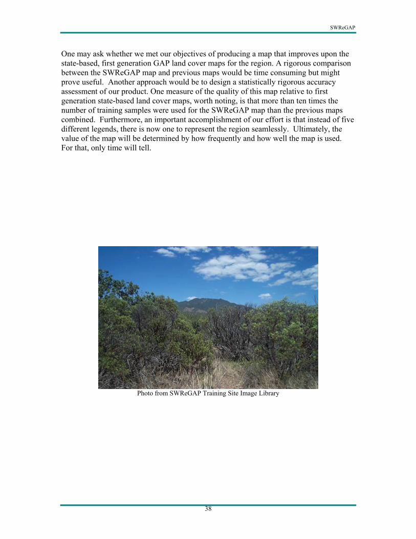
Photo from SWReGAP Training Site Image Library