Embed Size (px)
Citation preview
BSIM2EKVBSIM2EKV::BSIM3.3 to EKV2v6 Model Library File BSIM3.3 to EKV2v6 Model Library File
Automatic Conversion ToolAutomatic Conversion Tool
D. Stefanovic, F. Krummenacher, M. Pastre, M. Kayal
Swiss Federal Institute of Technology, Electronic Labs, STI/IMM/LEG, Lausanne, Switzerland
BSIM2EKV - D. Stefanovic, F. Krummenacher, M. Pastre, M. Kayal
BSIM2EKV converter
• Tool for automatic conversion of BSIM (version 3.3) model parametersto EKV (version 2.6) model parameters
• Standalone application (works in interaction with an external simulator)
• Basic principle of the conversion:
• the curves needed for the parameters extraction are simulated using the BSIM model library file
• the extraction procedure is based on the complete EKVmodel parameters extraction methodology
[ M. Bucher, C. Lallement, C.C. Enz, “An efficient parameter extraction methodology for the EKV MOSTmodel”, International Conference on Microelectronic Test Structures, ICMTS 1996, 25-28 March 1996, pp: 145 – 150 ]
BSIM2EKV - D. Stefanovic, F. Krummenacher, M. Pastre, M. Kayal
EKV model
• Dedicated to the design of analog circuits
• Strongly based on device physics
• Has a small number of parameters, but very good accuracy
http://legwww.epfl.ch/ekv
BSIM2EKV - D. Stefanovic, F. Krummenacher, M. Pastre, M. Kayal
EKV model
• Facilitates intuitive understanding of analog structures behavior
• Enables to find solutions for different input parameters sets withoutusing complex numerical methods
• Enables the extraction of transistor parameters important for analog design, such as:
inversion factor, saturation voltage, Early voltage, small signal parameters, parasitic capacitances, gm/ID ratio, transconductance efficiency factor
http://legwww.epfl.ch/ekv
BSIM2EKV - D. Stefanovic, F. Krummenacher, M. Pastre, M. Kayal
BSIM model
• Industrial standard - BSIM (version 3.3)
• Good accuracy
• Large number of parameters
• High complexity
http://www-device.eecs.berkeley.edu/~bsim
?Hand calculationsApproximationsgm/ID ratio, inversion factor
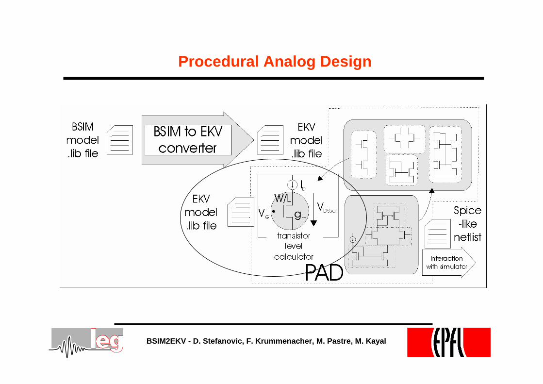
Procedural Analog Design
BSIM2EKV - D. Stefanovic, F. Krummenacher, M. Pastre, M. Kayal
BSIM2EKV - D. Stefanovic, F. Krummenacher, M. Pastre, M. Kayal
BSIM to EKV conversion
Opens new possibilities to use:
• EKV model (more extensively)
• CAD tools based on EKV model
• gm/Id design methodology
BSIM2EKV - D. Stefanovic, F. Krummenacher, M. Pastre, M. Kayal
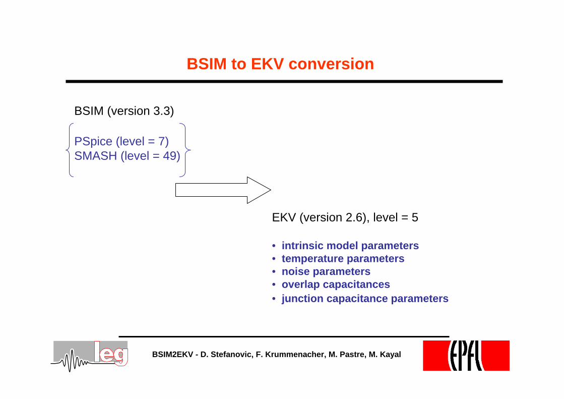
BSIM to EKV conversion
PSpice (level = 7)SMASH (level = 49)
EKV (version 2.6), level = 5
• intrinsic model parameters• temperature parameters• noise parameters• overlap capacitances• junction capacitance parameters
BSIM (version 3.3)
BSIM2EKV - D. Stefanovic, F. Krummenacher, M. Pastre, M. Kayal
Conversion algorithm
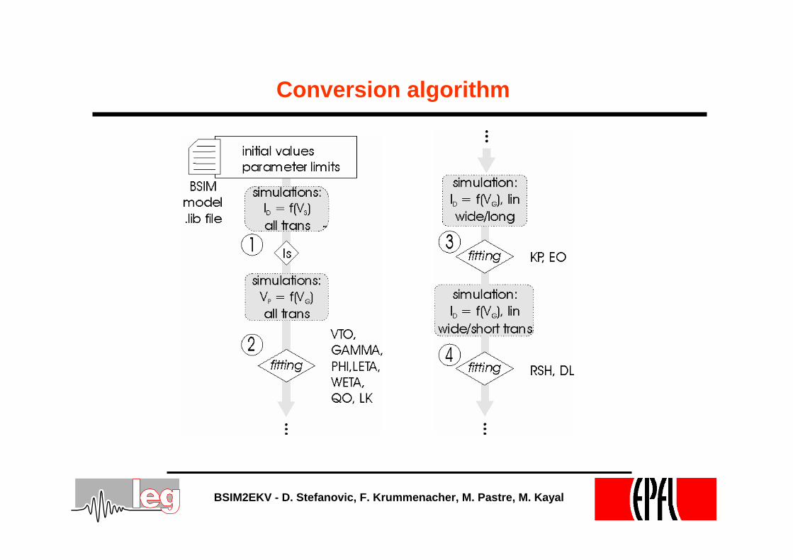
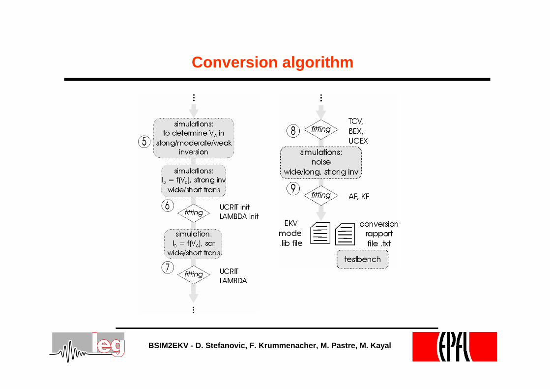
Basic concept:
• The curves required for the extraction procedure are simulated using the BSIM model
• Precise sequence of operations
• Minimum error propagation with the respect of fundaments of two models
BSIM2EKV - D. Stefanovic, F. Krummenacher, M. Pastre, M. Kayal
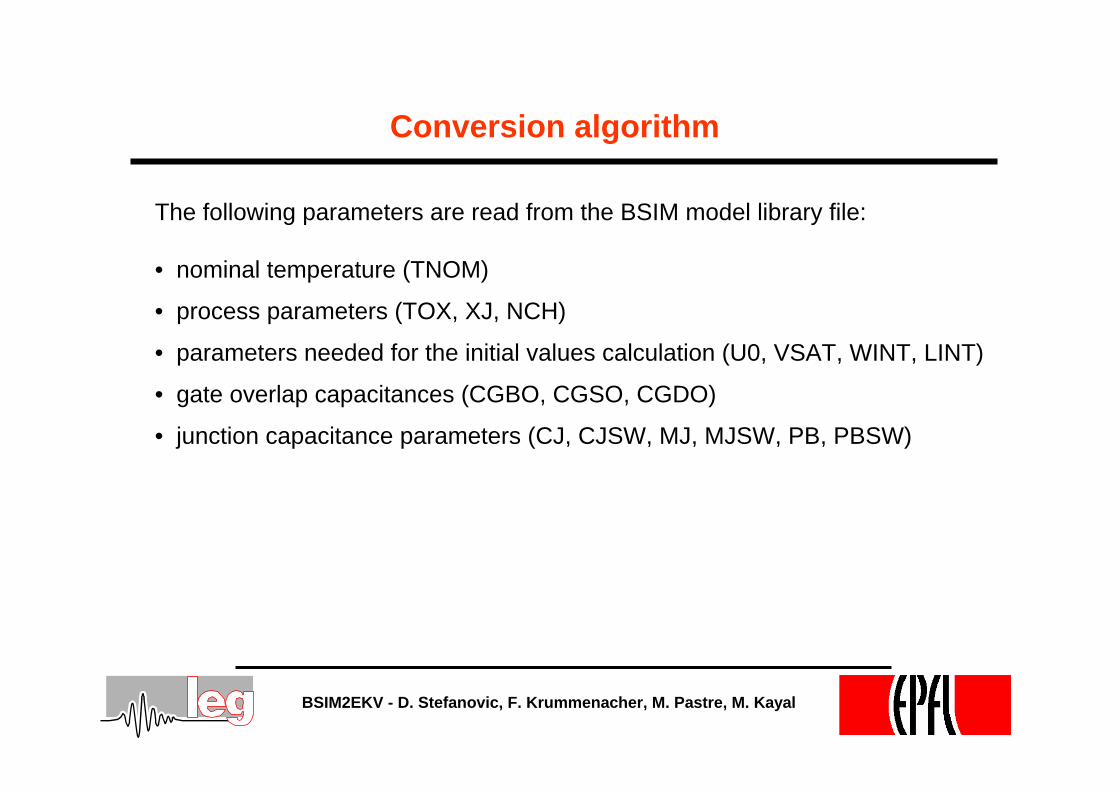
Conversion algorithm
The following parameters are read from the BSIM model library file:
• nominal temperature (TNOM)
• process parameters (TOX, XJ, NCH)
• parameters needed for the initial values calculation (U0, VSAT, WINT, LINT)
• gate overlap capacitances (CGBO, CGSO, CGDO)
• junction capacitance parameters (CJ, CJSW, MJ, MJSW, PB, PBSW)
BSIM2EKV - D. Stefanovic, F. Krummenacher, M. Pastre, M. Kayal
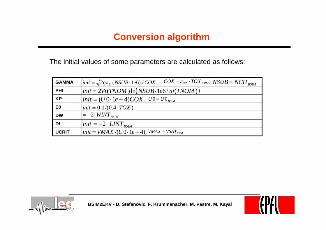
Conversion algorithm
The initial values of some parameters are calculated as follows:
UCRIT
DL
DW
E0
KP
PHI
GAMMA ,/)61(2 COXeNSUBqinit Si ⋅= ε ,/ BSIMOX TOXCOX ε=BSIMNCHNSUB =
( ))(/61ln)(2 TNOMnieNSUBTNOMVtinit ⋅=,)410( COXeUinit −⋅= BSIMUU 00 =
)4.0/(1.0 TOXinit ⋅=BSIMWINT⋅−= 2
BSIMLINTinit ⋅−= 2),410/( −⋅= eUVMAXinit BSIMVSATVMAX =
BSIM2EKV - D. Stefanovic, F. Krummenacher, M. Pastre, M. Kayal
Conversion algorithm
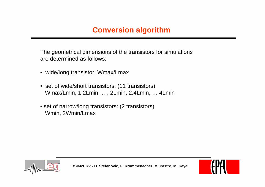
The geometrical dimensions of the transistors for simulationsare determined as follows:
• wide/long transistor: Wmax/Lmax
• set of wide/short transistors: (11 transistors)Wmax/Lmin, 1.2Lmin, …, 2Lmin, 2.4Lmin, … 4Lmin
• set of narrow/long transistors: (2 transistors) Wmin, 2Wmin/Lmax
BSIM2EKV - D. Stefanovic, F. Krummenacher, M. Pastre, M. Kayal
Conversion algorithm
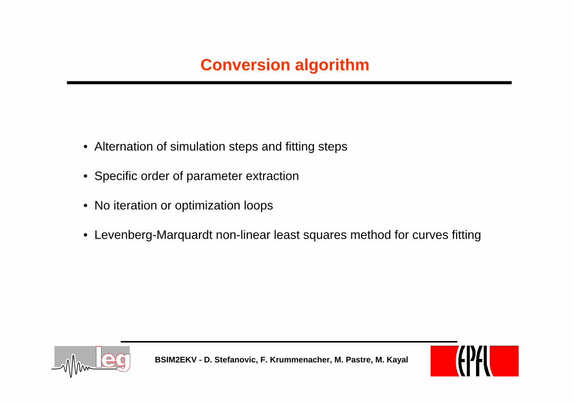
• Alternation of simulation steps and fitting steps
• Specific order of parameter extraction
• No iteration or optimization loops
• Levenberg-Marquardt non-linear least squares method for curves fitting
BSIM2EKV - D. Stefanovic, F. Krummenacher, M. Pastre, M. Kayal
Conversion algorithm
BSIM2EKV - D. Stefanovic, F. Krummenacher, M. Pastre, M. Kayal
Conversion algorithm
BSIM2EKV - D. Stefanovic, F. Krummenacher, M. Pastre, M. Kayal
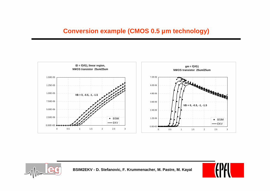
Conversion example (CMOS 0.5 µm technology)
ID = f(VG), linear region, NMOS transistor 25um/25um
0.00E+00
2.50E-06
5.00E-06
7.50E-06
1.00E-05
1.25E-05
1.50E-05
0 0.5 1 1.5 2 2.5 3
BSIMEKV
VB = 0, -0.5, -1, -1.5
gm = f(VG)NMOS transistor 25um/25um
0.0E+00
1.2E-06
2.4E-06
3.6E-06
4.8E-06
6.0E-06
7.2E-06
0 0.5 1 1.5 2 2.5 3
BSIMEKV
VB = 0, -0.5, -1, -1.5
BSIM2EKV - D. Stefanovic, F. Krummenacher, M. Pastre, M. Kayal
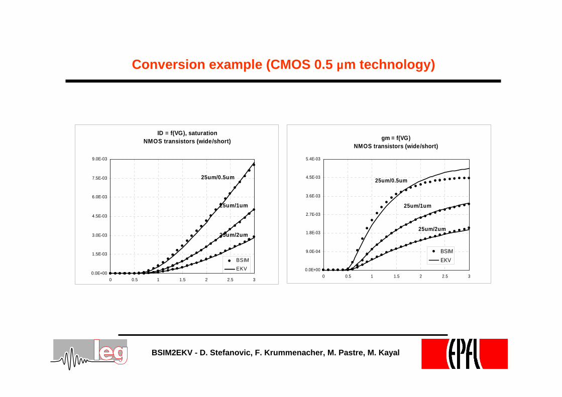
Conversion example (CMOS 0.5 µm technology)
ID = f(VG), saturationNMOS transistors (wide/short)
0.0E+00
1.5E-03
3.0E-03
4.5E-03
6.0E-03
7.5E-03
9.0E-03
0 0.5 1 1.5 2 2.5 3
BSIMEKV
25um/0.5um
25um/1um
25um/2um
gm = f(VG)NMOS transistors (wide/short)
0.0E+00
9.0E-04
1.8E-03
2.7E-03
3.6E-03
4.5E-03
5.4E-03
0 0.5 1 1.5 2 2.5 3
BSIMEKV
25um/0.5um
25um/1um
25um/2um
BSIM2EKV - D. Stefanovic, F. Krummenacher, M. Pastre, M. Kayal
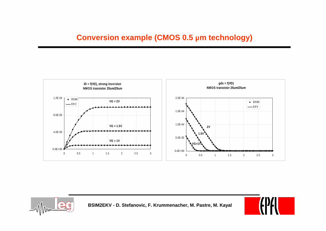
Conversion example (CMOS 0.5 µm technology)
ID = f(VD), strong inversionNMOS transistor 25um/25um
0.0E+00
4.0E-05
8.0E-05
1.2E-04
0 0.5 1 1.5 2 2.5 3
BSIMEKV
VG = 2V
VG = 1.5V
VG = 1V
gds = f(VD)NMOS transistor 25um/25um
0.0E+00
5.0E-05
1.0E-04
1.5E-04
2.0E-04
0 0.5 1 1.5 2 2.5 3
BSIMEKV
VG=1V
1.5V
2V
BSIM2EKV - D. Stefanovic, F. Krummenacher, M. Pastre, M. Kayal
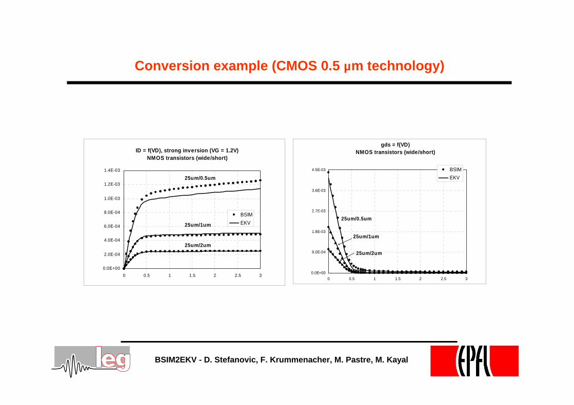
Conversion example (CMOS 0.5 µm technology)
ID = f(VD), strong inversion (VG = 1.2V)NMOS transistors (wide/short)
0.0E+00
2.0E-04
4.0E-04
6.0E-04
8.0E-04
1.0E-03
1.2E-03
1.4E-03
0 0.5 1 1.5 2 2.5 3
BSIMEKV
25um/0.5um
25um/1um
25um/2um
gds = f(VD)NMOS transistors (wide/short)
0.0E+00
9.0E-04
1.8E-03
2.7E-03
3.6E-03
4.5E-03
0 0.5 1 1.5 2 2.5 3
BSIMEKV
25um/0.5um
25um/1um
25um/2um
BSIM2EKV - D. Stefanovic, F. Krummenacher, M. Pastre, M. Kayal
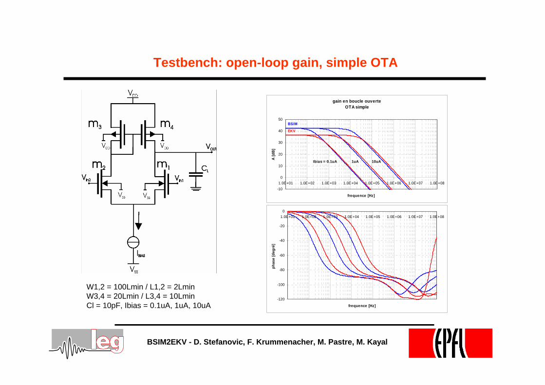
Testbench: open-loop gain, simple OTA
W1,2 = 100Lmin / L1,2 = 2LminW3,4 = 20Lmin / L3,4 = 10LminCl = 10pF, Ibias = 0.1uA, 1uA, 10uA
gain en boucle ouverteOTA simple
-10
0
10
20
30
40
50
1.0E+01 1.0E+02 1.0E+03 1.0E+04 1.0E+05 1.0E+06 1.0E+07 1.0E+08
frequence [Hz]
A [d
B]
Ibias = 0.1uA 1uA 10uA
BSIM
EKV
-120
-100
-80
-60
-40
-20
01.0E+01 1.0E+02 1.0E+03 1.0E+04 1.0E+05 1.0E+06 1.0E+07 1.0E+08
frequence [Hz]
phas
e [d
egré
]
BSIM2EKV - D. Stefanovic, F. Krummenacher, M. Pastre, M. Kayal
Conclusion
• EKV model – model dedicated to the design of analog circuits
• BSIM model – empirical model, widely used
• BSIM2EKV – enables to generate the EKV model parametersfrom BSIM model parameters (within several minutes)and opens new possibilities to use:
EKV model
PAD
gm/Id design methodology