Embed Size (px)
Citation preview
LUND UNIVERSITY
PO Box 117221 00 Lund+46 46-222 00 00
Swirl stabilized premixed flame analysis using of LES and POD
Iudiciani, Piero
2012
Link to publication
Citation for published version (APA):Iudiciani, P. (2012). Swirl stabilized premixed flame analysis using of LES and POD.
General rightsUnless other specific re-use rights are stated the following general rights apply:Copyright and moral rights for the publications made accessible in the public portal are retained by the authorsand/or other copyright owners and it is a condition of accessing publications that users recognise and abide by thelegal requirements associated with these rights. • Users may download and print one copy of any publication from the public portal for the purpose of private studyor research. • You may not further distribute the material or use it for any profit-making activity or commercial gain • You may freely distribute the URL identifying the publication in the public portal
Read more about Creative commons licenses: https://creativecommons.org/licenses/Take down policyIf you believe that this document breaches copyright please contact us providing details, and we will removeaccess to the work immediately and investigate your claim.
Swirl stabilized premixed flameanalysis using LES and POD
Piero Iudiciani
Department of Energy Science
Division of Fluid Mechanics
Faculty of Engineering, LTH
Lund University, Lund, Sweden
Akademisk avhandling som for avlaggande av teknologie doktorsexamen vid tekniska
fakulteten vid Lunds Universitet kommer att offentligen forsvaras onsdagen den 25
april 2012, kl. 10.15 i horsal M:B, pa M-huset, Ole Romers vag 1, Lund.
Fakultetsopponent: Dr. Sebastien Ducruix, (Ecole Centrale Paris / CNRS, Frankrike)
Academic thesis which, by due permission of the Faculty of Engineering at Lund
University, will be publicly defended on Wednesday 25 April, 2012, at 10.15 a.m.
in lecture hall M:B, in the M-bulding, Ole Romers vag 1, Lund, for the degree of
Doctor of Philosophy in Engineering.
Faculty opponent: Dr. Sebastien Ducruix, (Ecole Centrale Paris / CNRS, France)
Thesis for the degree of Doctor of Philosophy in Engineering.
ISBN 978-91-7473-281-8
ISSN 0282-1990
ISRN LUTMDN/TMHP-12/1086-SE
c©Piero Iudiciani, March 29, 2012
Department of Energy Sciences, Division of Fluid Mechanics
Lund Institute of Technology
Box 118, 22100 Lund, Sweden
Typeset in LATEX
Printed by E-husets Tryckeri, Lund, March 2012
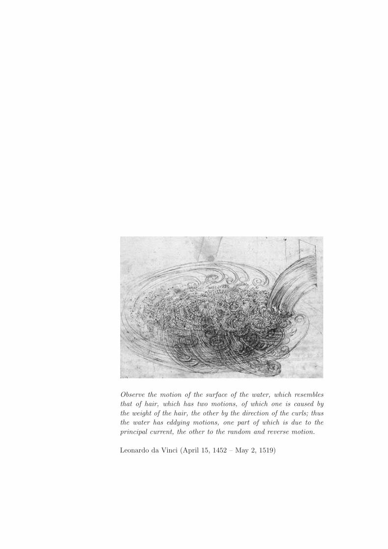
Observe the motion of the surface of the water, which resembles
that of hair, which has two motions, of which one is caused by
the weight of the hair, the other by the direction of the curls; thus
the water has eddying motions, one part of which is due to the
principal current, the other to the random and reverse motion.
Leonardo da Vinci (April 15, 1452 – May 2, 1519)

Abstract
For environmental and human health reasons, the regulations on the emissions from
combustion devices are getting more and more strict. In particular, it is important
to abate the emission of pollutants deriving from combustion in gas turbines. A
solution is the use of swirl stabilized, lean premixed combustion. Besides the ben-
eficial effects, there are still some issues related to instabilities and a full, clear
understanding of the dynamics of swirling flows and flames has not been reached
yet. This is where the contribution of this thesis lie. In this work, advanced tech-
niques, namely Large Eddy Simulation (LES), Proper Orthogonal Decomposition
(POD), and optical diagnostics, have been applied to analyze swirl stabilized flames,
relevant to gas turbine applications.
A simple geometry combustor, the “Lisbon”burner, useful for fundamental stud-
ies, was simulated by LES. The dynamics of a forced swirling flame are successfully
captured, allowing to characterize the influence of the Precessing Vortex Core on
the flame stabilization and its interactions with axial fluctuations.
However, real applications are typically characterized by more complex ge-
ometry. Special attention was then paid to the study of a realistic burner, the
“Triple Annular Research Swirler (TARS)”. Detailed LES of this aeroengine-like
fuel-injector, including the upstream portion of it, shed some light on the experi-
mentally observed asymmetry of the flow. The flow through the fuel-injector, un-
accessible to experiments, was clarified and detailed. Differences and similarities
with academic simple geometry swirl burners were also highlighted. For reacting
conditions, the LES formulation was able to explain the peculiar stabilization mech-
anism in a case where the CRZ was destroyed by thermal expansion, to capture dual
behavior/hysteresis phenomena, to describe the dynamics of a lean flame and its
interaction with the PVC.
Throughout the thesis, POD analysis highlighted large scale structures and
flame fluctuations of several combustors contributing to the understanding of the
dynamics of swirl stabilized flames.
It was shown how POD can relate to conditional averaging and in particular
to phase averaging. A POD based phase averaging procedure was used to study
thermo-acoustic oscillations. Applied to experimental data obtained with a simple
and relatively cheap set-up, but complex geometry and flow, it opens possibilities
for application on industrial rigs, enabling phase averaging with a priori unknown
period.
The concept of Extended POD was expanded to combustion applications high-
lighting the correlations between flow and flame dynamics. For both numerical and
experimental data, it gave new insights into flames and their correlation with the
flow field.

Contents
1 Introduction 1
1.1 Energy situation . . . . . . . . . . . . . . . . . . . . . . . . . . . . . 1
1.2 Gas turbines . . . . . . . . . . . . . . . . . . . . . . . . . . . . . . . 1
1.3 Swirling flows in gas turbines . . . . . . . . . . . . . . . . . . . . . . 3
1.4 Problems and challenges . . . . . . . . . . . . . . . . . . . . . . . . . 3
1.5 Strategy and solutions . . . . . . . . . . . . . . . . . . . . . . . . . . 4
1.6 Thesis contribution . . . . . . . . . . . . . . . . . . . . . . . . . . . . 5
1.7 Thesis outline . . . . . . . . . . . . . . . . . . . . . . . . . . . . . . . 5
2 Turbulent reacting flows 7
2.1 Phenomenological description of turbulence . . . . . . . . . . . . . . 7
2.1.1 Laminar and turbulent flows . . . . . . . . . . . . . . . . . . 7
2.1.2 Turbulent scales and energy cascade . . . . . . . . . . . . . . 8
2.2 Combustion . . . . . . . . . . . . . . . . . . . . . . . . . . . . . . . . 10
2.2.1 Chemical oxidation reactions . . . . . . . . . . . . . . . . . . 10
2.2.2 Pollutant formation . . . . . . . . . . . . . . . . . . . . . . . 11
2.2.2.1 Carbon monoxide . . . . . . . . . . . . . . . . . . . 11
2.2.2.2 Nitrogen oxide . . . . . . . . . . . . . . . . . . . . . 12
2.2.2.3 Unburned hydrocarbons (UHC) . . . . . . . . . . . 13
2.3 Turbulent combustion . . . . . . . . . . . . . . . . . . . . . . . . . . 14
2.3.1 Phenomenological description of flames . . . . . . . . . . . . 14
2.3.1.1 Premixed and diffusion flames . . . . . . . . . . . . 14
2.3.1.2 Laminar and turbulent flames . . . . . . . . . . . . 14
2.3.1.3 Laminar premixed flames . . . . . . . . . . . . . . . 14
2.3.1.4 Turbulent premixed flames . . . . . . . . . . . . . . 16
2.4 LES of turbulent reacting flows . . . . . . . . . . . . . . . . . . . . . 18
2.4.1 Flow equations and boundary conditions . . . . . . . . . . . . 18
2.4.2 Averaged/filtered equations . . . . . . . . . . . . . . . . . . . 19
2.4.3 Turbulence modeling . . . . . . . . . . . . . . . . . . . . . . . 22
2.4.3.1 Smagorinsky Model . . . . . . . . . . . . . . . . . . 22
2.4.3.2 Scale Similarity Model . . . . . . . . . . . . . . . . . 23
2.4.3.3 Germano’s Dynamic model . . . . . . . . . . . . . . 23
2.4.3.4 Filtered Smagorinsky . . . . . . . . . . . . . . . . . 24
2.4.3.5 Implicit LES (ILES) . . . . . . . . . . . . . . . . . . 24
2.4.4 Closures for the other SGS terms . . . . . . . . . . . . . . . . 24
2.4.5 Combustion modeling . . . . . . . . . . . . . . . . . . . . . . 25
2.4.5.1 ILES . . . . . . . . . . . . . . . . . . . . . . . . . . 25
2.4.5.2 Thickened flame model . . . . . . . . . . . . . . . . 25
2.4.5.3 Filtered density function . . . . . . . . . . . . . . . 26
vi Contents
2.4.5.4 G-equation . . . . . . . . . . . . . . . . . . . . . . . 26
2.4.5.5 Progress variable; the c-equation . . . . . . . . . . . 27
2.4.5.6 Filtered flamelet model with tabulated chemistry . . 27
2.5 Stabilizaton and combustion instabilities . . . . . . . . . . . . . . . . 29
2.5.1 Swirl stabilization . . . . . . . . . . . . . . . . . . . . . . . . 29
2.5.1.1 Precessing Vortex Core . . . . . . . . . . . . . . . . 30
2.5.2 Thermo-acoustic instabilities . . . . . . . . . . . . . . . . . . 31
3 Methods 33
3.1 Numerical methods . . . . . . . . . . . . . . . . . . . . . . . . . . . . 33
3.1.1 Finite Difference . . . . . . . . . . . . . . . . . . . . . . . . . 33
3.1.1.1 In-house solver details . . . . . . . . . . . . . . . . . 37
3.1.2 Finite Volume . . . . . . . . . . . . . . . . . . . . . . . . . . . 37
3.1.2.1 Accuracy of the schemes in OpenFOAM . . . . . . . 39
3.1.2.2 OpenFOAM details and scalability . . . . . . . . . . 39
3.2 Experimental techniques . . . . . . . . . . . . . . . . . . . . . . . . . 41
3.2.1 Particle Image Velocimetry . . . . . . . . . . . . . . . . . . . 41
3.2.2 Laser Induced Fluorescence . . . . . . . . . . . . . . . . . . . 42
3.2.3 Chemiluminescence . . . . . . . . . . . . . . . . . . . . . . . . 43
3.3 Proper Orthogonal Decomposition . . . . . . . . . . . . . . . . . . . 43
3.3.1 POD . . . . . . . . . . . . . . . . . . . . . . . . . . . . . . . . 43
3.3.2 Extended POD . . . . . . . . . . . . . . . . . . . . . . . . . . 45
3.3.3 Time coefficients information and interlink with phase averaging 45
4 Problem Set-up 49
4.1 Lisbon burner . . . . . . . . . . . . . . . . . . . . . . . . . . . . . . . 49
4.1.1 Computational domain and boundary conditions . . . . . . . 50
4.2 TARS . . . . . . . . . . . . . . . . . . . . . . . . . . . . . . . . . . . 51
4.2.1 TARS burner . . . . . . . . . . . . . . . . . . . . . . . . . . . 51
4.2.2 Burner support facility and diagnostic systems . . . . . . . . 53
4.2.3 Computational Domain and boundary conditions . . . . . . . 53
4.2.4 Summary of operating conditions . . . . . . . . . . . . . . . . 55
5 Summary of results 57
5.1 Lisbon burner . . . . . . . . . . . . . . . . . . . . . . . . . . . . . . . 57
5.1.1 Statistics . . . . . . . . . . . . . . . . . . . . . . . . . . . . . 57
5.1.2 POD analysis . . . . . . . . . . . . . . . . . . . . . . . . . . . 57
5.1.3 EPOD analysis . . . . . . . . . . . . . . . . . . . . . . . . . . 59
5.2 TARS . . . . . . . . . . . . . . . . . . . . . . . . . . . . . . . . . . . 61
5.2.1 Details of the flow inside the TARS by LES . . . . . . . . . . 62
5.2.1.1 Instantaneous flow . . . . . . . . . . . . . . . . . . . 62
5.2.1.2 Statistics and origin of the asymmetry . . . . . . . . 62
5.2.1.3 PVC identification by means of POD . . . . . . . . 64
Contents vii
5.2.2 Thermo-acoustic instability analysis by POD based phase av-
eraging . . . . . . . . . . . . . . . . . . . . . . . . . . . . . . 66
5.2.2.1 Statistics . . . . . . . . . . . . . . . . . . . . . . . . 66
5.2.2.2 POD analysis . . . . . . . . . . . . . . . . . . . . . . 67
5.2.2.3 POD based phase averaging . . . . . . . . . . . . . 68
6 Summary of the papers and author contribution 71
7 Conclusions and future work 75
7.1 Conclusions . . . . . . . . . . . . . . . . . . . . . . . . . . . . . . . . 75
7.2 Future work . . . . . . . . . . . . . . . . . . . . . . . . . . . . . . . . 76
Bibliography 79

Chapter 1
Introduction
1.1 Energy situation
In order to sustain the current living standards of modern society, the world’s energy
demand is constantly increasing. Although, in the future, a larger contribution from
renewable and sustainable sources is expected, it is foreseen that a great part of
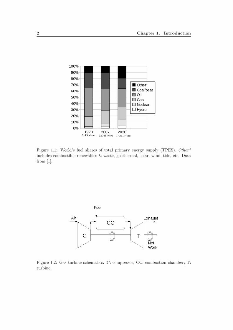
energy will still be produced by means of combustion, as sketched in Fig. 1.1 [1].
Moreover, the recent progresses in green-technologies enable today to partly replace
fossil fuels with synthetic renewable hydrocarbons [2]. Therefore combustion is still,
and so it will be in years to come, a vital technology for our modern society to
convert these fuels into work or electricity. One of the main problems related to
combustion are pollutants, harmful for the environment and for the human health,
and green-house gases, contributing to global warming. Among all the various
combustion applications, the gas turbine is often described as the prime mover of our
time [3]. It finds an increasingly wide variety of applications, the main ones being
electrical power generation or mechanical drive for land stationary gas turbines,
propulsion in the case of aeronautical engines. Further research is needed in order
to reduce the undesired emissions of combustion devices: carbon monoxide (CO),
unburned hydrocarbons (UHC), soot and especially nytrogen oxides (NOX) [4]. In
particular for stationary gas turbines, ultralow NOX operation has even become a
major marketing issue [3].
1.2 Gas turbines
A typical sketch of a gas turbine is reported in Fig. 1.2. In the schematics of Fig.
1.2, the flow goes from left to the right. It is composed by three main components,
a compressor, a combustor and a turbine. The pressure of the incoming flow is first
increased through the compressor. The air is then conveyed into the combustion
chamber, where fuel is added and burnt. The chemical energy of the fuel is converted
into heat, increasing the energy (temperature) of the gas. These burnt gases at high
temperature then expand through the turbine. Part of the energy is used to drive
the compressor, and the remaining part is the useful energy. In stationary gas
turbines it is used to drive a mechanical load or an electricity generator, while in
aero-engines the flow further expands for giving propulsion.
This thesis aims at contributing to the part of the process in which the air and
fuel are mixed and burnt in the combustion chamber. As it will be clarified in
Section 2.3.1.1, there are two main modes of combustion: premixed, in which air
2 Chapter 1. Introduction
Figure 1.1: World’s fuel shares of total primary energy supply (TPES). Other*
includes combustible renewables & waste, geothermal, solar, wind, tide, etc. Data
from [1].
Figure 1.2: Gas turbine schematics. C: compressor; CC: combustion chamber; T:
turbine.
1.3. Swirling flows in gas turbines 3
and fuel are blended together before the combustion takes place, and non-premixed
(diffusion type) in which the fuel and air are injected separately and mix directly
into the combustion chamber. To reduce the level of the emissions, it is important
to reduce the temperature of the flame, as it will be explained later in Section 2.2.2.
Premixed flames are thus desirable, because they allow a better control of the flame
temperature, and consequently of emissions. At the present time lean premixed
(LP) combustion appears to be the only technology available for achieving ultralow
NOx emissions from practical combustors [3,5]. When dealing with liquid fuels, one
should rather talk about lean premixed prevaporized (LPP) [6] combustion.
1.3 Swirling flows in gas turbines
In the design of modern lean premixed combustors, swirling flows play an important
role. Vortex breakdown [7] is nowadays the preferred flame holding mechanism.
Swirl stabilized flames are rather compact and allow the design of smaller and
lighter combustion chambers. Moreover there is the advantage that no flame holders
are needed in the hot regions of the flame (and therefore no need to cool them).
The incoming fresh mixture is given a swirling motion which induces a recirculating
bubble in the center of the jet. This Central Recirculation Zone (CRZ), recirculating
hot burnt gases, provides the heat necessary to preheat and ignite the incoming
air-fuel mixture. Moreover, swirling flows enhance mixing of the fuel with the
air flow, both for gaseous and liquid fuels. In particular liquid fuels need to be
atomized, vaporized and mixed. Complex swirling flows with azimuthal shear layers
and vortex breakdown allow rapid mixing over a short length. Therefore, fuel-
injectors with multiple swirlers are typically used when atomization utilizes airblast
atomizers [5] (Fuel is atomized by shear with the incoming high speed flow, another
possibility is to inject fuel at high-pressure, so called pressure atomizers [5]).
1.4 Problems and challenges
LP combustion allows to reduce the peak temperature, avoiding the formation of
pollutants, but stability issues arise. Typical problems are flashback [8, 9], blow-
off [8, 10], thermo-acoustic oscillations [11–16], combustion noise [17, 18]. When
operating at very lean conditions, the peak temperature in the combustor becomes
lower, whereby lowering the NOx emissions levels. On the other hand, providing less
heat to the fresh gases, lean flames are susceptible to quenching or flame blow-out.
Typical dynamics related to vortex breakdown [19], such as helical structures [20],
Precessing Vortex Core (PVC) [21–25], can be a source of unsteady flow and heat
release which may trigger instabilities such as thermo-acoustic oscillations (coupling
between pressure and heat release fluctuations). Although they have been used and
studied for several decades, swirling flows are still an open field of research. To
address the stability issues mentioned above, understanding the dynamics of vortex
breakdown and swirl-stabilized flames is crucial.
4 Chapter 1. Introduction
1.5 Strategy and solutions
In recent years, strong efforts have been made both experimentally and numerically
to improve the knowledge of the related phenomena and to explore ideas for cir-
cumventing flame stability issues in LPP combustors. For example, the dynamic
response to axial oscillations of both non-reacting [22, 26–31] and reacting [32–39]
swirling flows has been analyzed. The work presented in this thesis has the main
goal to contribute to the better understanding of swirling flows and flames. This
has been done by using advanced numerical and experimental techniques. Special
emphasis has been put on numerical computations by means of Large Eddy Simu-
lation (LES) [40]. LES allows to resolve the major fraction of the turbulent kinetic
energy and to capture the unsteady motion of large scale structures. Thereby, it
is believed to be indispensable if one wants to address the stability and the dy-
namics of flow/flames. Large scale coherent structures have been found to have
an important role in raising flame instabilities because interacting with the flame
they can drive heat release fluctuations [32, 41, 42]. LES provides a rather large
amount of data which has to be processed. Normally, one uses statistical tools to
characterize the random turbulent fluctuations. The most energetic fraction of the
fluctuations can be identified using Proper Orthogonal Decomposition (POD) [43].
POD is a well established technique for the analysis and control of cold turbulent
flows [44–47], but recently has also gained interest for its application to reacting
flows [18, 24, 39, 48–55]. This thesis also aims at encouraging the use of POD as
a tool to analize reacting flows and in particular to improve the understanding of
flame dynamics. This modal decomposition can be applied to either numerical or
experimental data, to extract the fluctuations of the different variables of interest
(velocity field, OH-signal, OH-chemiluminesce, etc.) as a set of ”modes”. Highlight-
ing relevant flow and flame dynamics, it is a powerful tool to investigate the flame
stability. Recent POD-derived techniques, such as POD based a-posteriori phase
averaging [56, 57], and Extended POD (EPOD) [58, 59] (see Section 3.3) may then
open new possibilities. The application of EPOD to reacting flows is particularly
interesting: correlating variables representing the reaction zone (progress variable,
species, temperature, etc.) with the velocity field, the interactions between flow
and flame dynamics can be highlighted.
Usually, to investigate fundamental phenomena, one tries to reduce the problem
to the study of simple geometry, downscaled laboratory apparatus, an idealized re-
production of reality. We cite here a few examples [22,26,60]. Such an approach is
indeed very instructive to gain general knowledge, isolate the phenomena, or to vali-
date models. We followed this “modus operandi”in the case of Paper I [61], in which
the interaction of PVC and longitudinal oscillations is studied in a simple geometry
swirler, the “Lisbon”burner [23, 60], and in Paper II [62], where a simple laminar
Bunsen flame interacting with acoustics is used to exemplify the use of EPOD in
combustion applications. However, since the reality is much more complicated, it is
not guaranteed that the results obtained in such idealized situations can be extra-
polated to actual industrial applications. Many factors neglected or removed in a
1.6. Thesis contribution 5
laboratory can play an important role. For example, more complex geometries are
typically used. For this reason, the thesis also studies flows and flames generated
through a complex device, the Triple Annular Research Swirler, TARS [63], a model
gas turbine fuel-injector, mimicking the ones used in propulsion applications. The
investigations of this burner are given in Papers III-VI. Paper III [64] clarifies the
complex flow inside and outside the TARS; Paper IV [65] proposes a method for
the analysis of thermo-acoustic instabilities in industrial rigs, Paper V [66] explains
the stabilization mechanism for a case without central recirculation zone and Paper
VI [67] focuses on the dynamics of a very lean flame.
1.6 Thesis contribution
The main achievements accomplished with the work of this thesis are listed below:
• The dynamics of a forced swirling flame are successfully captured by means of
LES, allowing to characterize the influence of the PVC motion on the flame
stabilization and its interactions with axial fluctuations.
• Proper Orthogonal Decomposition highlighted large scale structures and flame
fluctuations of several combustors contributing to the understanding of the
dynamics of swirling flames.
• POD based a-posteriori phase averaging was used to study thermo-acoustic
oscillations. Applied to experimental data obtained with a simple and rela-
tively cheap (for example compared to laser diagnostics) set-up, but complex
geometry and flow, it opens possibilities for application on industrial rigs,
enabling phase averaging with a priori unknown period.
• The concept of Extended POD was expanded to combustion applications high-
lighting the correlations between flow and flame dynamics. For both numerical
and experimental data, it gave new insights into flames and their correlation
with the flow field.
• More detailed LES of the TARS burner including the upstream portion of it,
shed some light on the experimentally observed asymmetry of the flow.
1.7 Thesis outline
This thesis is organized as a collection of the papers which have been produced
during this project. The articles are preceded by an introductory overview of the
topics which are not treated in details in the papers. In Chapter 2 the theoretical
background about turbulence, combustion, turbulent combustion and flame stabi-
lization is briefly treated. In Chapter 3 the methods used to collect and process the
information (LES, experimental diagnostics, POD-EPOD) are described. Chapter
4 contains a description of the test cases studied in this work, i.e. the Lisbon and

6 Chapter 1. Introduction
the TARS burners. A summary of the main results is reported in Chapter 5. The
detailed results are found in the papers appended at the end of the book. Chap-
ter 6 summarizes the content of each paper together with the contribution of the
candidate to the paper itself. In Chapter 7 the main conclusions of this work are
resumed, together with proposals for future investigations.
Chapter 2
Turbulent reacting flows
2.1 Phenomenological description of turbulence
2.1.1 Laminar and turbulent flows
Most of the flows in industrial applications are turbulent. A turbulent flow is
characterized by the fact of being irregular, random and chaotic. A classic way to
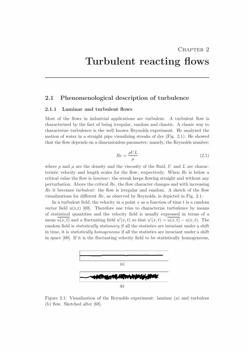
characterize turbulence is the well known Reynolds experiment. He analyzed the
motion of water in a straight pipe visualizing streaks of dye (Fig. 2.1). He showed
that the flow depends on a dimensionless parameter; namely, the Reynolds number:
Re =ρUL
µ(2.1)
where ρ and µ are the density and the viscosity of the fluid, U and L are charac-
teristic velocity and length scales for the flow, respectively. When Re is below a
critical value the flow is laminar : the streak keeps flowing straight and without any
perturbation. Above the critical Re, the flow character changes and with increasing
Re it becomes turbulent : the flow is irregular and random. A sketch of the flow
visualizations for different Re, as observed by Reynolds, is depicted in Fig. 2.1.
In a turbulent field, the velocity in a point x as a function of time t is a random
vector field u(x,t) [69]. Therefore one tries to characterize turbulence by means
of statistical quantities and the velocity field is usually expressed in terms of a
mean u(x, t) and a fluctuating field u′(x, t) so that u′(x, t) = u(x, t) − u(x, t). The
random field is statistically stationary if all the statistics are invariant under a shift
in time, it is statistically homogeneous if all the statistics are invariant under a shift
in space [69]. If it is the fluctuating velocity field to be statistically homogeneous,
Figure 2.1: Visualization of the Reynolds experiment: laminar (a) and turbulent
(b) flow. Sketched after [68].
8 Chapter 2. Turbulent reacting flows
one talks about homogenous turbulence: turbulence is statistically the same in all
the points. If the statistics of the fluctuating field are invariant under rotations or
reflections of the coordinate system, one talks about isotropic turbulence [69] (i.e.
directionally independent).
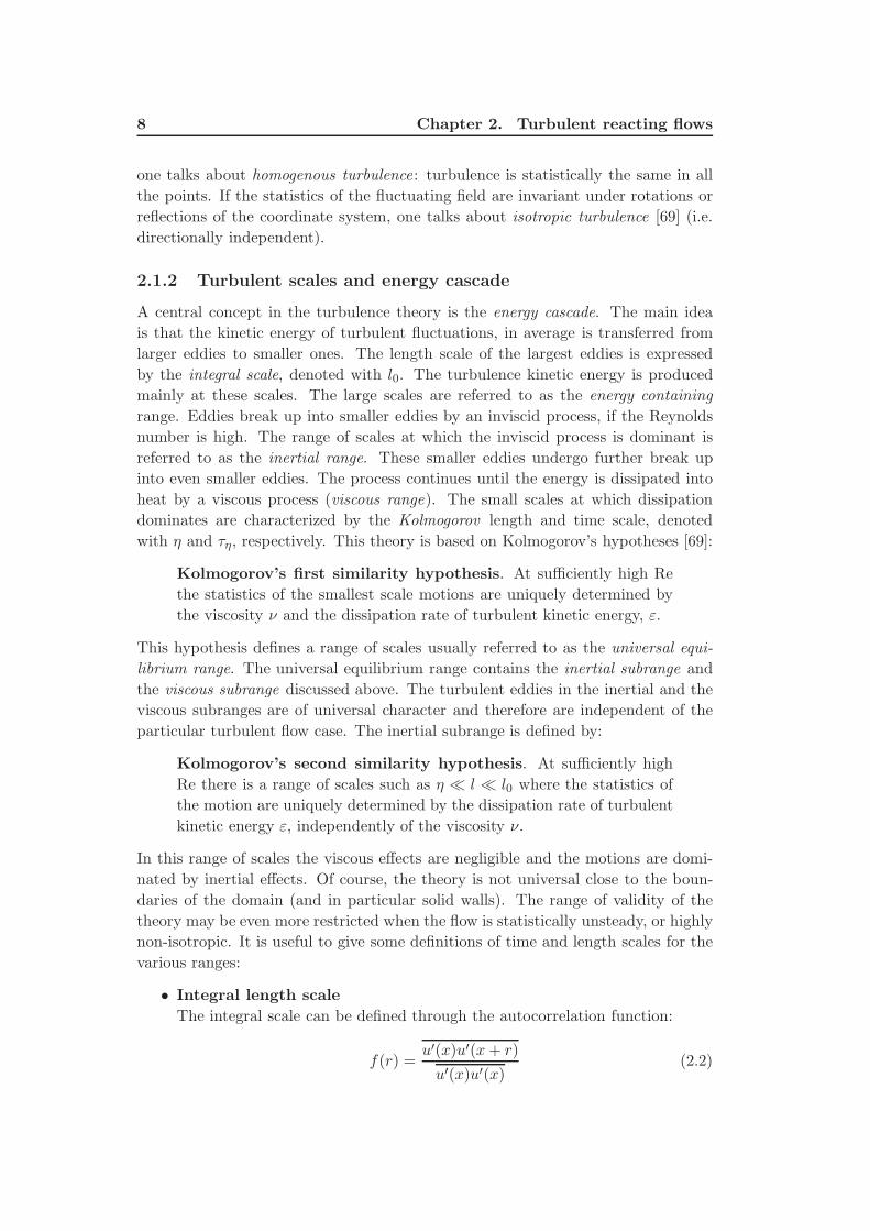
2.1.2 Turbulent scales and energy cascade
A central concept in the turbulence theory is the energy cascade. The main idea
is that the kinetic energy of turbulent fluctuations, in average is transferred from
larger eddies to smaller ones. The length scale of the largest eddies is expressed
by the integral scale, denoted with l0. The turbulence kinetic energy is produced
mainly at these scales. The large scales are referred to as the energy containing
range. Eddies break up into smaller eddies by an inviscid process, if the Reynolds
number is high. The range of scales at which the inviscid process is dominant is
referred to as the inertial range. These smaller eddies undergo further break up
into even smaller eddies. The process continues until the energy is dissipated into
heat by a viscous process (viscous range). The small scales at which dissipation
dominates are characterized by the Kolmogorov length and time scale, denoted
with η and τη, respectively. This theory is based on Kolmogorov’s hypotheses [69]:
Kolmogorov’s first similarity hypothesis. At sufficiently high Re
the statistics of the smallest scale motions are uniquely determined by
the viscosity ν and the dissipation rate of turbulent kinetic energy, ε.
This hypothesis defines a range of scales usually referred to as the universal equi-
librium range. The universal equilibrium range contains the inertial subrange and
the viscous subrange discussed above. The turbulent eddies in the inertial and the
viscous subranges are of universal character and therefore are independent of the
particular turbulent flow case. The inertial subrange is defined by:
Kolmogorov’s second similarity hypothesis. At sufficiently high
Re there is a range of scales such as η ≪ l ≪ l0 where the statistics of
the motion are uniquely determined by the dissipation rate of turbulent
kinetic energy ε, independently of the viscosity ν.
In this range of scales the viscous effects are negligible and the motions are domi-
nated by inertial effects. Of course, the theory is not universal close to the boun-
daries of the domain (and in particular solid walls). The range of validity of the
theory may be even more restricted when the flow is statistically unsteady, or highly
non-isotropic. It is useful to give some definitions of time and length scales for the
various ranges:
• Integral length scale
The integral scale can be defined through the autocorrelation function:
f(r) =u′(x)u′(x+ r)
u′(x)u′(x)(2.2)
2.1. Phenomenological description of turbulence 9
where u′(x) is the velocity fluctuation in a point and r is the distance from
the point x, the overbar indicates time average. The integral length scale is
then defined as the integral of the autocorrelation function:
l0 =
∫∞
0f(r) dr (2.3)
and it represents the mean distance at which the fluctuations are correlated,
a memory effect in space.
• Taylor scale
The Taylor scale can be defined from the second derivative of the autocorre-
lation function at r=0, as follows:
λ2f = − 2d2fdr2|r=0
(2.4)
Taylor thought that this length scale could roughly describe the diameter of
the smallest eddies responsible for dissipation. However, this happens at the
Kolmogorov scales. The Taylor length scale has no clear physical interpre-
tation [69], but it is useful in practical applications since it typically falls in
the inertial subrange. Thus, this scale can be used to estimate the required
spatial resolution for LES.
• Kolmogorov scale
The Kolmogorov scales are the smallest turbulent scales. The length, time
and velocity scales, are denoted with η, τη and uη respectively. These are
expressed by:
η =
(ν3
ε
) 1
4
, τη =(νε
) 1
2
, uη = (εν)1
4 (2.5)
Using these scales the turbulent Reynolds numberReη =uηην = 1, consistently
with the fact that the behavior is universal.
Assuming equilibrium between production of turbulent kinetic energy and dis-
sipation, it is possible to derive relations between the integral and Kolmogorov
scales [69]:η
l0∼ Re− 3
4 ,τητ0∼ Re− 1
2 (2.6)
where Re is the turbulent Reynolds number (based on velocity and length scales of
the eddies). Therefore the Kolmogorov length scale decreases with increasing Re.
For a typical gas turbine, assuming Re ≃ 106 and l0 ≃ 0.1m, it is of the order of
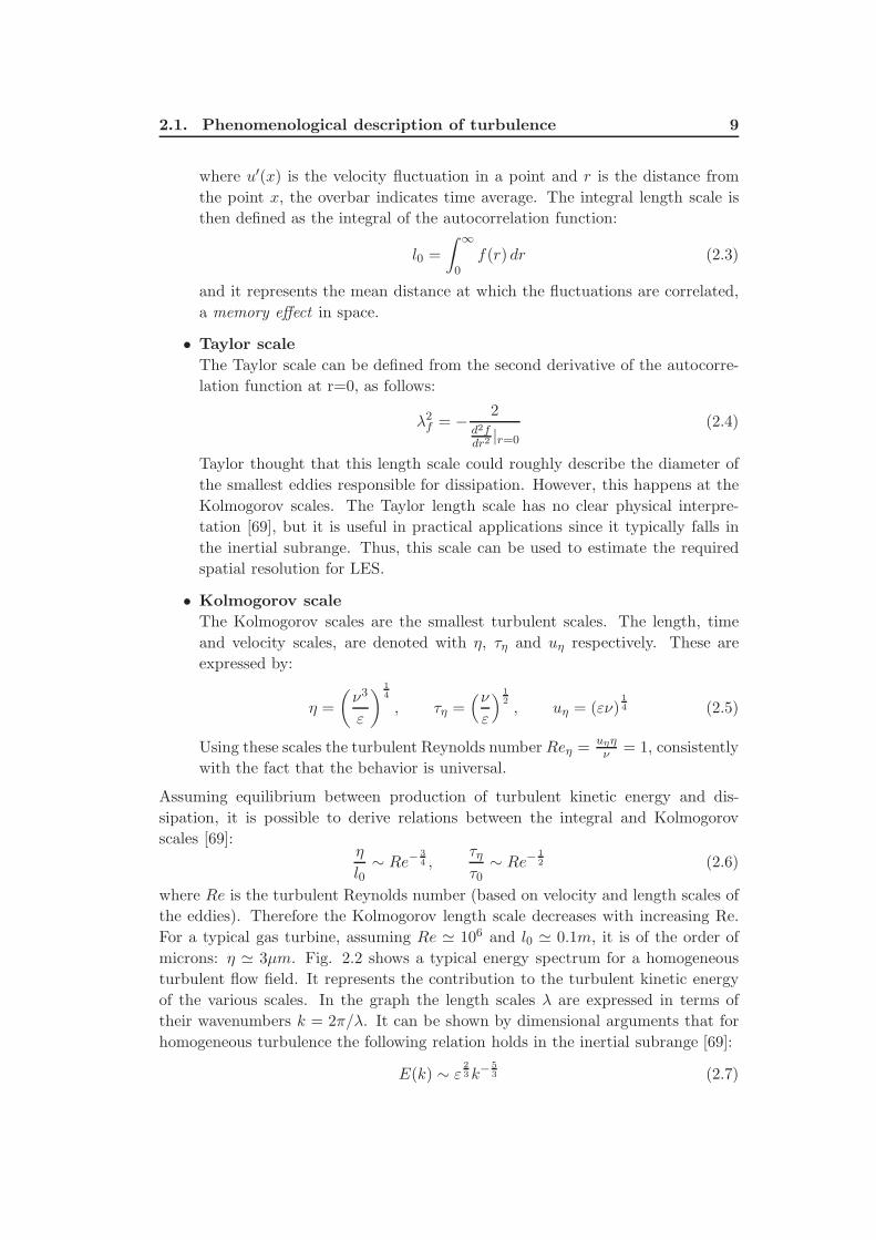
microns: η ≃ 3µm. Fig. 2.2 shows a typical energy spectrum for a homogeneous
turbulent flow field. It represents the contribution to the turbulent kinetic energy
of the various scales. In the graph the length scales λ are expressed in terms of
their wavenumbers k = 2π/λ. It can be shown by dimensional arguments that for
homogeneous turbulence the following relation holds in the inertial subrange [69]:
E(k) ∼ ε 2
3k−5
3 (2.7)
10 Chapter 2. Turbulent reacting flows
Figure 2.2: Energy spectrum as a function of wave number. Sketched after [70].
2.2 Combustion
2.2.1 Chemical oxidation reactions
Combustion is a chemical process which involves chemical oxidation reactions in
gas phase. A generic chemical reaction can be described as follows:
NS∑
i=1
ν ′iYi ←→NS∑
i=1
ν ′′i Yi (2.8)
where Yi represents the generic chemical species and ν ′i, ν′′
i are respectively the
stoichiometric coefficients of the reactants and the products. The rate at which the
reaction occurs is often given by the Arrhenius law:
K = AT be−EaℜT (2.9)
where A and b are experimental parameters, Ea is the energy of activation, ℜ is
the universal gas constant and T is the temperature. During combustion the fuel
reacts with the oxidizer (in general air or pure oxygen) to form products, and a
certain amount of heat is released (exotermic reaction). Typical fuels in industrial
applications are hydrocarbons burning in air or oxygen. The combustion process is
commonly described with one or a very few global reactions. An example of one-step
global reaction in the case of methane-air combustion is:
CH4 + 202 = CO2 + 2H2O (2.10)
2.2. Combustion 11
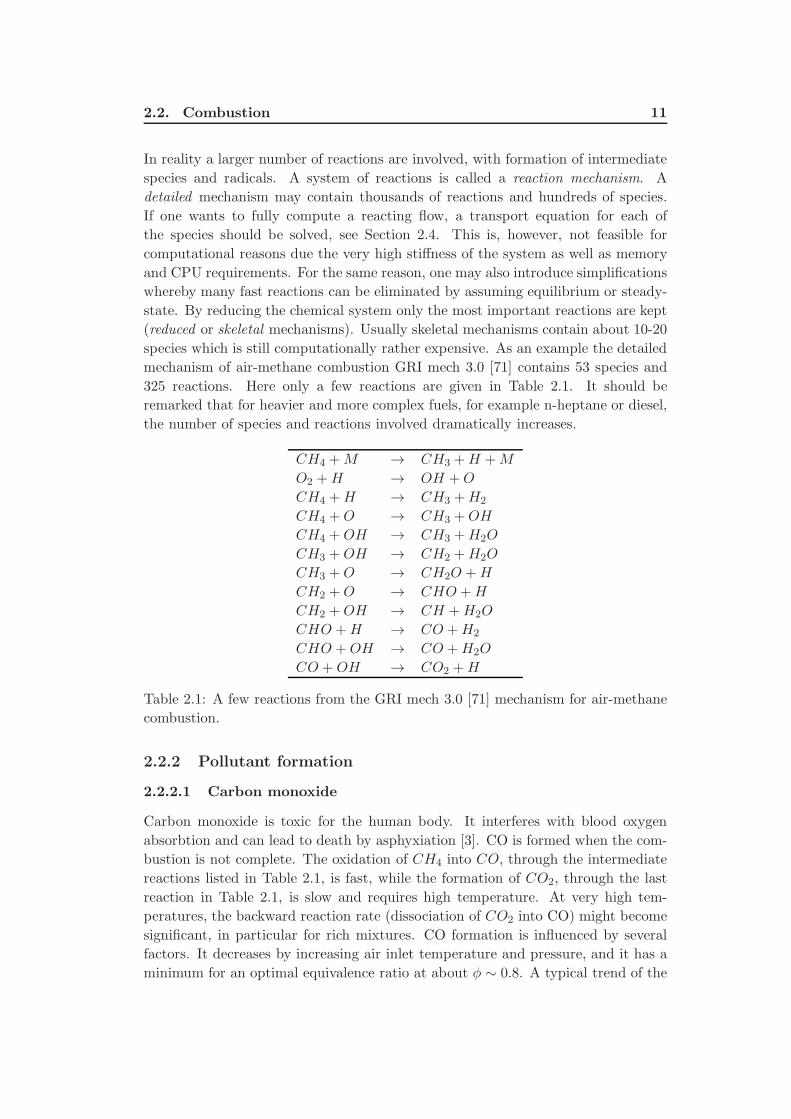
In reality a larger number of reactions are involved, with formation of intermediate
species and radicals. A system of reactions is called a reaction mechanism. A
detailed mechanism may contain thousands of reactions and hundreds of species.
If one wants to fully compute a reacting flow, a transport equation for each of
the species should be solved, see Section 2.4. This is, however, not feasible for
computational reasons due the very high stiffness of the system as well as memory
and CPU requirements. For the same reason, one may also introduce simplifications
whereby many fast reactions can be eliminated by assuming equilibrium or steady-
state. By reducing the chemical system only the most important reactions are kept
(reduced or skeletal mechanisms). Usually skeletal mechanisms contain about 10-20
species which is still computationally rather expensive. As an example the detailed
mechanism of air-methane combustion GRI mech 3.0 [71] contains 53 species and
325 reactions. Here only a few reactions are given in Table 2.1. It should be
remarked that for heavier and more complex fuels, for example n-heptane or diesel,
the number of species and reactions involved dramatically increases.
CH4 +M → CH3 +H +M
O2 +H → OH +O
CH4 +H → CH3 +H2
CH4 +O → CH3 +OH
CH4 +OH → CH3 +H2O
CH3 +OH → CH2 +H2O
CH3 +O → CH2O +H
CH2 +O → CHO +H
CH2 +OH → CH +H2O
CHO +H → CO +H2
CHO +OH → CO +H2O
CO +OH → CO2 +H
Table 2.1: A few reactions from the GRI mech 3.0 [71] mechanism for air-methane
combustion.
2.2.2 Pollutant formation
2.2.2.1 Carbon monoxide
Carbon monoxide is toxic for the human body. It interferes with blood oxygen
absorbtion and can lead to death by asphyxiation [3]. CO is formed when the com-
bustion is not complete. The oxidation of CH4 into CO, through the intermediate
reactions listed in Table 2.1, is fast, while the formation of CO2, through the last
reaction in Table 2.1, is slow and requires high temperature. At very high tem-
peratures, the backward reaction rate (dissociation of CO2 into CO) might become
significant, in particular for rich mixtures. CO formation is influenced by several
factors. It decreases by increasing air inlet temperature and pressure, and it has a
minimum for an optimal equivalence ratio at about φ ∼ 0.8. A typical trend of the
12 Chapter 2. Turbulent reacting flows
CO formation with the flame temperature is reported in Fig. 2.3 [3].
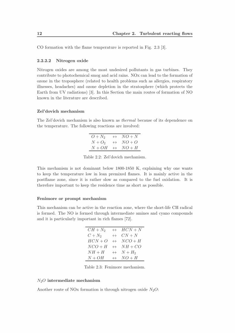
2.2.2.2 Nitrogen oxide
Nitrogen oxides are among the most undesired pollutants in gas turbines. They
contribute to photochemical smog and acid rains. NOx can lead to the formation of
ozone in the troposphere (related to health problems such as allergies, respiratory
illnesses, headaches) and ozone depletion in the stratosphere (which protects the
Earth from UV radiations) [3]. In this Section the main routes of formation of NO
known in the literature are described.
Zel’dovich mechanism
The Zel’dovich mechanism is also known as thermal because of its dependence on
the temperature. The following reactions are involved:
O +N2 ↔ NO +N
N +O2 ↔ NO +O
N +OH ↔ NO +H
Table 2.2: Zel’dovich mechanism.
This mechanism is not dominant below 1800-1850 K, explaining why one wants
to keep the temperature low in lean premixed flames. It is mainly active in the
postflame zone, since it is rather slow as compared to the fuel oxidation. It is
therefore important to keep the residence time as short as possible.
Fenimore or prompt mechanism
This mechanism can be active in the reaction zone, where the short-life CH radical
is formed. The NO is formed through intermediate amines and cyano compounds
and it is particularly important in rich flames [72].
CH +N2 ↔ HCN +N
C +N2 ↔ CN +N
HCN +O ↔ NCO +H
NCO +H ↔ NH + CO
NH +H ↔ N +H2
N +OH ↔ NO +H
Table 2.3: Fenimore mechanism.
N2O intermediate mechanism
Another route of NOx formation is through nitrogen oxide N2O:
2.2. Combustion 13
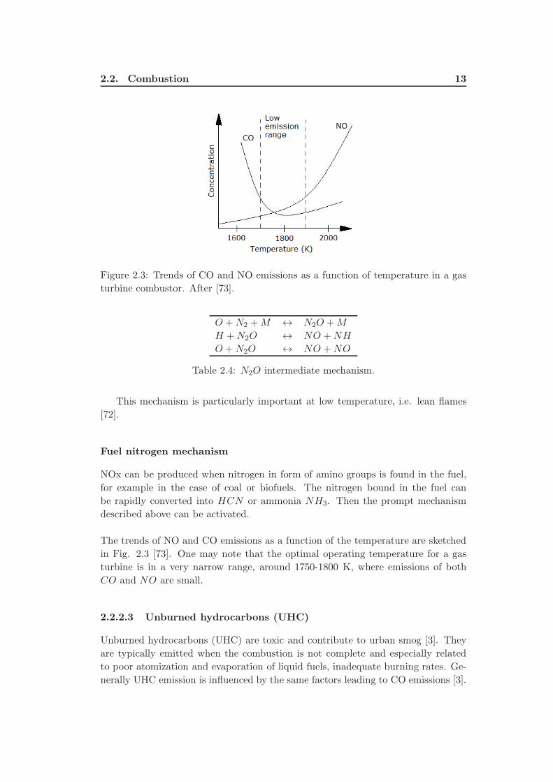
Figure 2.3: Trends of CO and NO emissions as a function of temperature in a gas
turbine combustor. After [73].
O +N2 +M ↔ N2O +M
H +N2O ↔ NO +NH
O +N2O ↔ NO +NO
Table 2.4: N2O intermediate mechanism.
This mechanism is particularly important at low temperature, i.e. lean flames
[72].
Fuel nitrogen mechanism
NOx can be produced when nitrogen in form of amino groups is found in the fuel,
for example in the case of coal or biofuels. The nitrogen bound in the fuel can
be rapidly converted into HCN or ammonia NH3. Then the prompt mechanism
described above can be activated.
The trends of NO and CO emissions as a function of the temperature are sketched
in Fig. 2.3 [73]. One may note that the optimal operating temperature for a gas
turbine is in a very narrow range, around 1750-1800 K, where emissions of both
CO and NO are small.
2.2.2.3 Unburned hydrocarbons (UHC)
Unburned hydrocarbons (UHC) are toxic and contribute to urban smog [3]. They
are typically emitted when the combustion is not complete and especially related
to poor atomization and evaporation of liquid fuels, inadequate burning rates. Ge-
nerally UHC emission is influenced by the same factors leading to CO emissions [3].
14 Chapter 2. Turbulent reacting flows
2.3 Turbulent combustion
2.3.1 Phenomenological description of flames
A flame is a mode of combustion [72]. One talks about a flame when combustion
occurs in a thin reaction layer propagating into a flow. A flame is also character-
ized by light emission. However, combustion may occur without light radiation:
distributed in a volume (flameless or mild combustion [74–76]), or on a surface
(catalytic combustion).
2.3.1.1 Premixed and diffusion flames
Flames can be distinguished according to the way fuel and oxidizer are mixed to-
gether. When fuel and oxidizer are mixed before entering the combustion chamber
one talks about premixed flames. In Non-premixed or diffusion flames instead,
fuel and oxidizer enter the combustion chamber separately and mix together in the
reaction zone. The way fuel and oxidizer are mixed affects the flame structure.
Premixed flames are desirable because they allow better temperature control, and
therefore enabling low NOx emissions. Diffusion flames always have regions in which
fuel and oxidizer are in stoichiometric proportion. They are therefore characterized
by higher temperatures, which is bad both in terms of emissions and soot formation.
2.3.1.2 Laminar and turbulent flames
Flames can be also characterized by the Reynolds number. Depending on the nature
of the flow, one distinguishes between laminar and turbulent flames. Laminar flames
are interesting from an academic point of view to understand elementary combustion
phenomena. The main impact of turbulence is on the burning rate: turbulent
flames ensure faster burning and are therefore popular in industrial applications
and in particular in gas turbines. This thesis focuses mainly on premixed turbulent
flames.
2.3.1.3 Laminar premixed flames
An important parameter to characterize premixed flames is the equivalence ratio Φ
of the fresh mixture. It is defined as:
Φ =(YF /YO)
(YF /YO)st(2.11)
where YF and YO are respectively the fuel and oxidizer mass fractions. The subscript
st indicates stoichiometric conditions (fuel and oxidizer in exact amount so that the
combustion is complete). The equivalence ratio tells how much fuel and oxidizer are
mixed with respect to theoretical stoichoimetric conditions. Φ < 1, Φ = 1 and Φ > 1
correspond to lean, stoichiometric and rich mixtures, respectively. For example
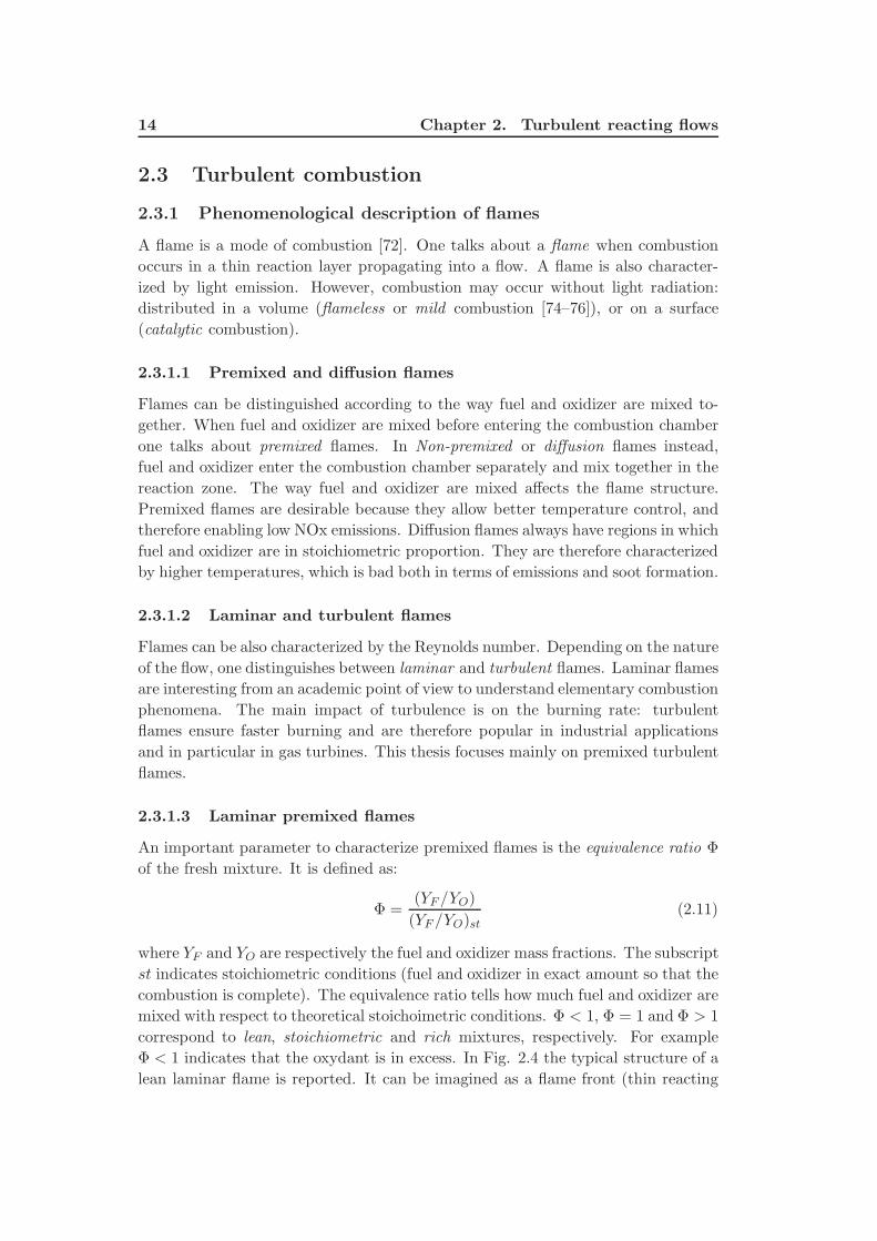
Φ < 1 indicates that the oxydant is in excess. In Fig. 2.4 the typical structure of a
lean laminar flame is reported. It can be imagined as a flame front (thin reacting
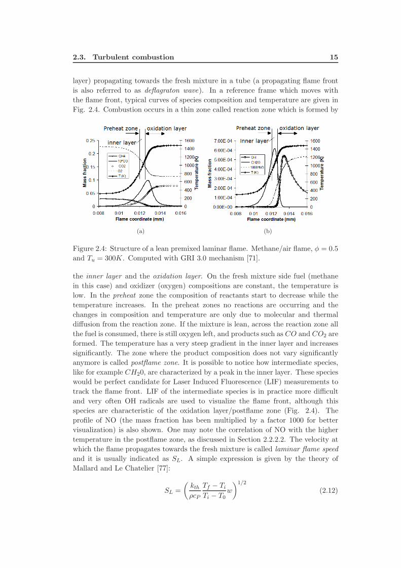
2.3. Turbulent combustion 15
layer) propagating towards the fresh mixture in a tube (a propagating flame front
is also referred to as deflagraton wave). In a reference frame which moves with
the flame front, typical curves of species composition and temperature are given in
Fig. 2.4. Combustion occurs in a thin zone called reaction zone which is formed by
(a) (b)
Figure 2.4: Structure of a lean premixed laminar flame. Methane/air flame, φ = 0.5
and Tu = 300K. Computed with GRI 3.0 mechanism [71].
the inner layer and the oxidation layer. On the fresh mixture side fuel (methane
in this case) and oxidizer (oxygen) compositions are constant, the temperature is
low. In the preheat zone the composition of reactants start to decrease while the
temperature increases. In the preheat zones no reactions are occurring and the
changes in composition and temperature are only due to molecular and thermal
diffusion from the reaction zone. If the mixture is lean, across the reaction zone all
the fuel is consumed, there is still oxygen left, and products such as CO and CO2 are
formed. The temperature has a very steep gradient in the inner layer and increases
significantly. The zone where the product composition does not vary significantly
anymore is called postflame zone. It is possible to notice how intermediate species,
like for example CH20, are characterized by a peak in the inner layer. These species
would be perfect candidate for Laser Induced Fluorescence (LIF) measurements to
track the flame front. LIF of the intermediate species is in practice more difficult
and very often OH radicals are used to visualize the flame front, although this
species are characteristic of the oxidation layer/postflame zone (Fig. 2.4). The
profile of NO (the mass fraction has been multiplied by a factor 1000 for better
visualization) is also shown. One may note the correlation of NO with the higher
temperature in the postflame zone, as discussed in Section 2.2.2.2. The velocity at
which the flame propagates towards the fresh mixture is called laminar flame speed
and it is usually indicated as SL. A simple expression is given by the theory of
Mallard and Le Chatelier [77]:
SL =
(kthρcP
Tf − TiTi − T0
w
)1/2
(2.12)
16 Chapter 2. Turbulent reacting flows
where kth is the thermal conductivity, cP is the specific heat, T0 and Ti are the
temperatures at the beginning and at the end of the preheat zone respectively,
Tf is the temperature at the exit of the reaction zone, w is the reaction rate.
It is important to remark that the laminar flame speed is a characteristic of the
mixture. SL has a maximum for Φ ≃ 1, because the temperature of the burnt gases
is maximum at stoichiometric conditions. At Φ = 1 combustion would be faster
but at the same time stoichiometric equivalence ratio is undesirable because of the
large NOx emission levels.
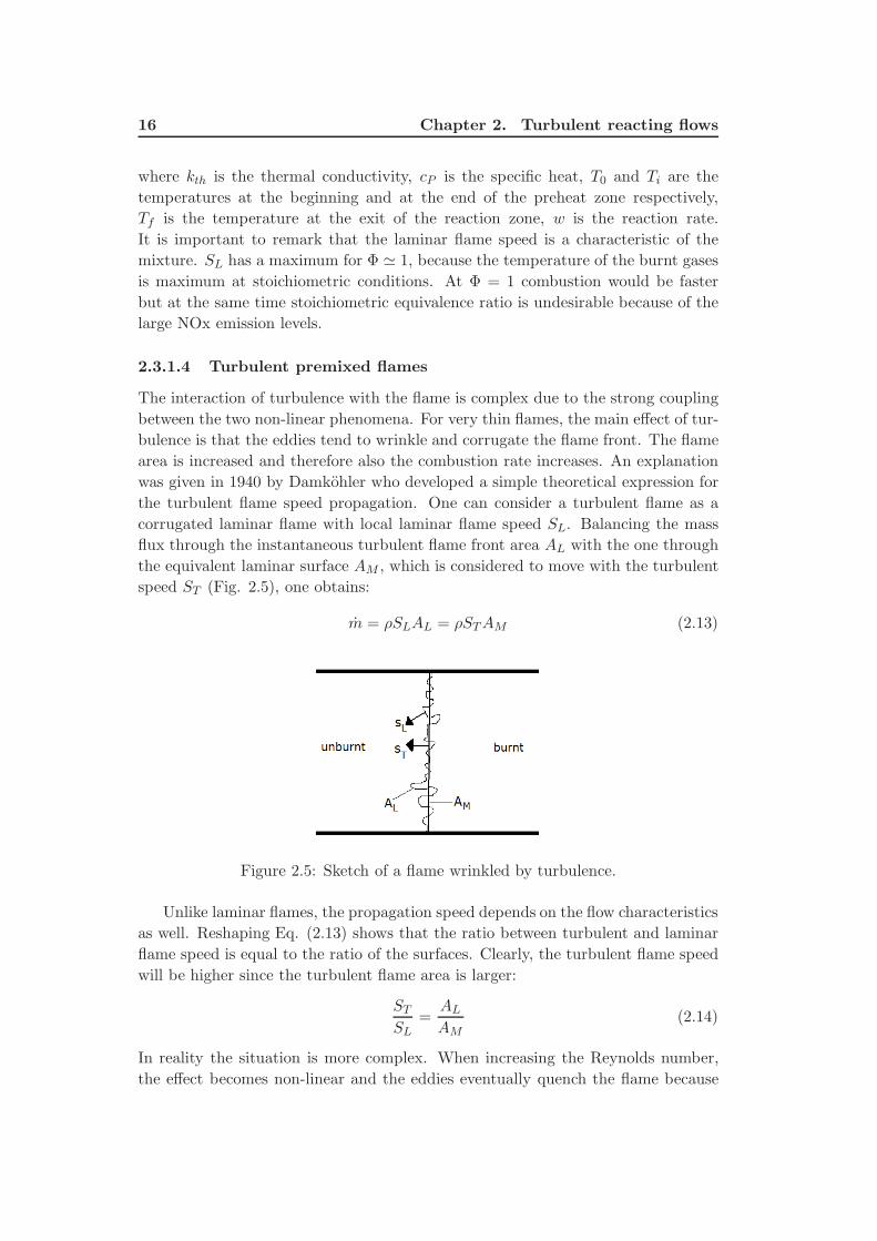
2.3.1.4 Turbulent premixed flames
The interaction of turbulence with the flame is complex due to the strong coupling
between the two non-linear phenomena. For very thin flames, the main effect of tur-
bulence is that the eddies tend to wrinkle and corrugate the flame front. The flame
area is increased and therefore also the combustion rate increases. An explanation
was given in 1940 by Damkohler who developed a simple theoretical expression for
the turbulent flame speed propagation. One can consider a turbulent flame as a
corrugated laminar flame with local laminar flame speed SL. Balancing the mass
flux through the instantaneous turbulent flame front area AL with the one through
the equivalent laminar surface AM , which is considered to move with the turbulent
speed ST (Fig. 2.5), one obtains:
m = ρSLAL = ρSTAM (2.13)
Figure 2.5: Sketch of a flame wrinkled by turbulence.
Unlike laminar flames, the propagation speed depends on the flow characteristics
as well. Reshaping Eq. (2.13) shows that the ratio between turbulent and laminar
flame speed is equal to the ratio of the surfaces. Clearly, the turbulent flame speed
will be higher since the turbulent flame area is larger:
STSL
=AL
AM(2.14)
In reality the situation is more complex. When increasing the Reynolds number,
the effect becomes non-linear and the eddies eventually quench the flame because
2.3. Turbulent combustion 17
of high shear and cooling. The flow field can then affect the flame in contrasting
ways. On the other hand, it is not only the turbulence affecting the flame, the
flame affects the flow as well. Across the flame the flow undergoes a quick change
in temperature, density, viscosity. The Reynolds number is reduced in the burnt
gases, which in some cases can lead to relaminarization, but because of the density
change across the flame, the flow is also strongly accelerated leading to instability.
These coupled non-linear phenomena are rather complex and depend on different
parameters [70]. Two non-dimensional numbers can be defined, the Damkohler
number Da and the Karlovitz number Ka. They both relate chemical and flow
time scales, but using different characteristic scales within the turbulent spectrum.
The Damkohler number is defined as the ratio between the integral time scale τ0and the chemical time scale τc. The integral time scale can be expressed as the
integral lenght scale l0 over the velocity fluctuations u′. Indicating with δL the
laminar flame thickness, the chemical time scale can be expressed as δLSL
, which
represents the time in which a laminar flame propagates over the distance of one
flame thickness. The Damkohler number is therefore [70]:
Da =τ0τc
=l0SLδLu′
(2.15)
The Karlovitz number instead compares the chemical time scale with the Kol-
mogorov time scale [70]:
Ka =τcτη
=δLuηηSL
=
(l0δL
)−
1
2
(u′
SL
) 3
2
(2.16)
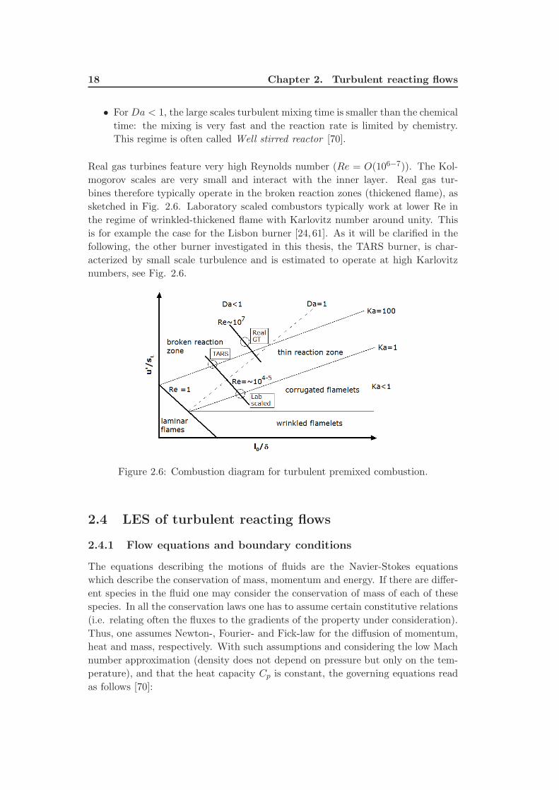
According to the values of these parameters, the behaviour of turbulent pre-
mixed flames can be characterized through a schematic diagram (known as Borghi’s
diagram, Fig. 2.6):
• In the bottom left corner of the diagram the Reynolds number is below 1 and
the regime is laminar
• When Ka < 1, the smallest eddies (Kolmogorov scales) are bigger than the
flame thickness. The eddies cannot enter the reaction layer and turbulence can
only wrinkle the laminar flame front. If u′ < SL the regime is called wrinkled
flamelets, if u′ > SL the regime is called corrugated flamelets: formation of
pockets of burnt and fresh gases is possible [70].
• When Ka > 1, the Kolmogorov eddies can interact with the flame. In the
range 1 < Ka < 100, the smallest eddies can interact with the preheat zone
but not with the inner layer: the reaction layer is thickened and this regime
is referred to as thin reaction zones, or thickened-wrinkled
• When Ka > 100 the Kolmogorov eddies can enter the inner layer. The
structure of the flame is not laminar anymore. This regime is called Broken
reaction zones or distributed combustion.
18 Chapter 2. Turbulent reacting flows
• ForDa < 1, the large scales turbulent mixing time is smaller than the chemical
time: the mixing is very fast and the reaction rate is limited by chemistry.
This regime is often called Well stirred reactor [70].
Real gas turbines feature very high Reynolds number (Re = O(106−7)). The Kol-
mogorov scales are very small and interact with the inner layer. Real gas tur-
bines therefore typically operate in the broken reaction zones (thickened flame), as
sketched in Fig. 2.6. Laboratory scaled combustors typically work at lower Re in
the regime of wrinkled-thickened flame with Karlovitz number around unity. This
is for example the case for the Lisbon burner [24, 61]. As it will be clarified in the
following, the other burner investigated in this thesis, the TARS burner, is char-
acterized by small scale turbulence and is estimated to operate at high Karlovitz
numbers, see Fig. 2.6.
Figure 2.6: Combustion diagram for turbulent premixed combustion.
2.4 LES of turbulent reacting flows
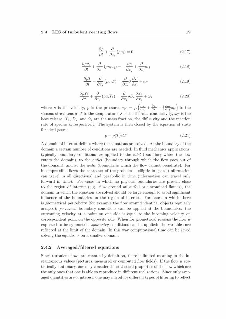
2.4.1 Flow equations and boundary conditions
The equations describing the motions of fluids are the Navier-Stokes equations
which describe the conservation of mass, momentum and energy. If there are differ-
ent species in the fluid one may consider the conservation of mass of each of these
species. In all the conservation laws one has to assume certain constitutive relations
(i.e. relating often the fluxes to the gradients of the property under consideration).
Thus, one assumes Newton-, Fourier- and Fick-law for the diffusion of momentum,
heat and mass, respectively. With such assumptions and considering the low Mach
number approximation (density does not depend on pressure but only on the tem-
perature), and that the heat capacity Cp is constant, the governing equations read
as follows [70]:
2.4. LES of turbulent reacting flows 19
∂ρ
∂t+
∂
∂xi(ρui) = 0 (2.17)
∂ρuj∂t
+∂
∂xi(ρuiuj) = −
∂p
∂xj+
∂
∂xiσij (2.18)
∂ρT
∂t+
∂
∂xi(ρuiT ) =
∂
∂xiλ∂T
∂xi+ ωT (2.19)
∂ρYk∂t
+∂
∂xi(ρuiYk) =
∂
∂xiρDk
∂Yk∂xi
+ ωk (2.20)
where u is the velocity, p is the pressure, σij = µ(
∂ui
∂xj+
∂uj
∂xi− 2
3∂uk
∂xkδij
)is the
viscous stress tensor, T is the temperature, λ is the thermal conductivity, ωT is the
heat release. Yk, Dk, and ωk are the mass fraction, the diffusivity and the reaction
rate of species k, respectively. The system is then closed by the equation of state
for ideal gases:
p = ρ(T )ℜT (2.21)
A domain of interest defines where the equations are solved. At the boundary of the
domain a certain number of conditions are needed. In fluid mechanics applications,
typically boundary conditions are applied to the inlet (boundary where the flow
enters the domain), to the outlet (boundary through which the flow goes out of
the domain), and at the walls (boundaries which the flow cannot penetrate). For
incompressible flows the character of the problem is elliptic in space (information
can travel in all directions) and parabolic in time (information can travel only
forward in time). For cases in which no physical boundaries are present close
to the region of interest (e.g. flow around an airfoil or unconfined flames), the
domain in which the equation are solved should be large enough to avoid significant
influence of the boundaries on the region of interest. For cases in which there
is geometrical periodicity (for example the flow around identical objects regularly
arrayed), periodical boundary conditions can be applied at the boundaries: the
outcoming velocity at a point on one side is equal to the incoming velocity on
correspondent point on the opposite side. When for geometrical reasons the flow is
expected to be symmetric, symmetry conditions can be applied: the variables are
reflected at the limit of the domain. In this way computational time can be saved
solving the equations on a smaller domain.
2.4.2 Averaged/filtered equations
Since turbulent flows are chaotic by definition, there is limited meaning in the in-
stantaneous values (pictures, measured or computed flow fields). If the flow is sta-
tistically stationary, one may consider the statistical properties of the flow which are
the only ones that one is able to reproduce in different realizations. Since only aver-
aged quantities are of interest, one may introduce different types of filtering to reflect
20 Chapter 2. Turbulent reacting flows
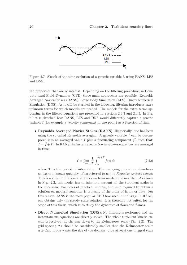
Figure 2.7: Sketch of the time evolution of a generic variable f, using RANS, LES
and DNS.
the properties that are of interest. Depending on the filtering procedure, in Com-
putational Fluid Dynamics (CFD) three main approaches are possible: Reynolds
Averaged Navier-Stokes (RANS), Large Eddy Simulation (LES), Direct Numerical
Simulation (DNS). As it will be clarified in the following, filtering introduces extra
unknown terms for which models are needed. The models for the extra terms ap-
pearing in the filtered equations are presented in Sections 2.4.3 and 2.4.5. In Fig.
2.7 it is sketched how RANS, LES and DNS would differently capture a generic
variable f (for example a velocity component in one point) as a function of time.
• Reynolds Averaged Navier Stokes (RANS): Historically, one has been
using the so called Reynolds averaging. A generic variable f can be decom-
posed into an averaged value f plus a fluctuating component f ′, such that:
f = f + f ′. In RANS the instantaneous Navier-Stokes equations are averaged
in time:
f = limT→∞
1
T
∫ t0+T
t0
f(t) dt (2.22)
where T is the period of integration. The averaging procedure introduces
an extra unknown quantity, often referred to as the Reynolds stresses tensor.
This is a closure problem and the extra term needs to be modeled. As shown
in Fig. 2.2, this model has to take into account all the turbulent scales in
the spectrum. For flows of practical interest, the time required to obtain a
solution on modern computer is typically of the order of hours or days. For
this reason RANS is the most popular CFD tool used in industry. In RANS,
one obtains only the steady state solution. It is therefore not suited for the
scope of this thesis, which is to study the dynamics of flows and flames.
• Direct Numerical Simulation (DNS): No filtering is performed and the
instantaneous equations are directly solved. The whole turbulent kinetic en-
ergy is resolved, all the way down to the Kolmogorov scale (Fig. 2.2). The
grid spacing ∆x should be considerably smaller than the Kolmogorov scale:
η ≫ ∆x. If one wants the size of the domain to be at least one integral scale
2.4. LES of turbulent reacting flows 21
l0, it is possible to estimate the minimum number of grid points N in each
direction, so that l0 = N∆x, through Eq. (2.6):
N > Re3/4 (2.23)
Since one solves the DNS equations in time, one needs also O(Re3/4) time
steps, all these leading to an operation count proportional to Re3. For the
high Reynolds numbers typical of practical applications, a very fine grid with
a large number of grid points is needed, and DNS is computationally not
feasible.
• Large Eddy Simulation (LES): In this case the instantaneous Navier
Stokes equations are filtered in space (either spectral or physical space):
f(x) =
∫f(x′)F∆(x− x′) dx′ (2.24)
where F∆(x) is the LES filter, of width ∆. Typical filters are the cut-off
filter in the spectral space, the top-hat or the Gaussian filter in the physical
space. After the filtering procedure, several unknown terms appear in the
equations, as it will be shown in the following. In LES, the filtered variable f
is solved for and the unclosed terms represent the unresolved subgrid scales
(SGS) fluctuations. The turbulent kinetic energy of the scales larger than the
width of the filter size is resolved (Fig. 2.2), while only the effect of turbulent
structures smaller than the filter (subgrid scales) needs to be modeled. Typical
models developed in the LES framework are summarized in Section 2.4.3.
Because of its capability to resolve in time a large fraction of the turbulent
kinetic energy, LES is a suitable tool to address the unsteady phenomena
object of this thesis. The price to be paid is in terms of computational time: a
typical run can require several weeks to obtain converged statistics. Although
it is still a tool which is mostly used in the academy, the interest of the
industry towards LES is constantly increasing.
For reacting flows, the density cannot be considered as a constant and to simplify
the equations Favre (density weighted) filtering is applied:
f =ρf
ρ(2.25)
Favre filtered quantities are indicated with a tilde and the density weighted filtering
operator is then expressed as:
ρf(x) =
∫ρf(x′)F∆(x− x′) dx′ (2.26)
A generic variable f can be decomposed into the Favre-filtered value f plus a
subgrid component f ′′, such that: f = f + f ′′. One should note that for filtering,
22 Chapter 2. Turbulent reacting flows
f ′′ 6= 0,˜ff ′′ 6= 0, f 6= ˜
f . It should be remarked that the exchange of the filtering
and derivative operation, ∂f∂x = ∂f
∂x , is not generally valid. The uncertainities due
to this operator are generally assumed to be included in the subgrid models [70].
Equations (2.17-2.21) are filtered and read [70]:
∂ρ
∂t+
∂
∂xi(ρui) = 0 (2.27)
∂ρuj∂t
+∂
∂xi(ρuiuj) +
∂p
∂xj=
∂
∂xi(σij + ρuiuj − ρuiuj) (2.28)
∂ρT
∂t+
∂
∂xi
(ρuiT
)=
∂
∂xi
(ρuiT − ρuiT + λ
∂T
∂xi
)+ ˜ωT (2.29)
∂ρYk∂t
+∂
∂xi
(ρuiYk
)=
∂
∂xi
(ρuiYk − ρuiYk + ρDk
∂Yk∂xi
)+ ˜ωk (2.30)
p = ¯ρ(T )ℜT (2.31)
2.4.3 Turbulence modeling
After the filtering procedure, several extra unknown terms appear in the equations.
In the momentum equation, the aforementioned SGS tensor appears, denoted as τij
τij = ρ (uiuj − uiuj) = ρuiuj − ρ(˜uiuj + u′′i uj +
˜uiu′′j + u′′i u′′
j
)(2.32)
In LES the model to close the momentum equation is less crucial than in RANS
because only the subgrid scale turbulence needs to be taken into account. The large
eddies, which depend strongly on the particular geometry, are resolved. In the LES
models, only a small fraction of the turbulent kinetic energy needs to be accounted
for and eventually, the finer the filter width, LES should tend to DNS. According to
the turbulent energy cascade theory, the kinetic energy is in average transferred to
the small scales where it is dissipated. Instantaneously, it can happen that energy
is transferred from small to larger scales (backscatter). One should express the SGS
stresses τij in terms of known filtered quantities, and a good SGS model should take
into account both dissipation and backscatter. Several models have been proposed
for the closure of the filtered equations. For more detailed discussions, the reader
is referred to [40,78]. A brief summary of the most popular LES models is given in
the following.
2.4.3.1 Smagorinsky Model
A typical approach to close the problem is to follow the Boussinesq ’s hypothesis.
The turbulent fluctuations increase the mixing and are modelled in analogy to the
2.4. LES of turbulent reacting flows 23
diffusion term. A turbulent viscosity µ∆ is introduced and the SGS stresses are
rewritten as
τij = ρ (uiuj − uiuj) = µ∆
(∂ui∂xj
+∂uj∂xi− 2
3
∂uk∂xk
δij
)(2.33)
The Smagorinsky model [79] is based on the Boussinesq’s hypothesis, and is a direct
extrapolation of earlier RANS models. The turbulent viscosity is expressed as:
µ∆ = ρ(CS∆)2|S| (2.34)
where ∆ is the filter width, CS is a constant, S is the filtered rate of strain. The
advantage of this model is its simplicity, which makes it very popular. It has
drawbacks: it is too dissipative, it does not account for backscatter, it overpredicts
viscosity near the walls, it does not converge to 0 for laminar flows.
2.4.3.2 Scale Similarity Model
The idea behind this model [80] is that the unresolved scales should behave similarly
to the resolved ones. In particular the assumption is that the most active subgrid
scales are those closer to the cutoff wave number, and that the scales with which
they interact most are those right above the cutoff [40]. A test filter wider than ∆
is introduced, denoted with a hat.
τij = ρ (uiuj − uiuj) = ρ(ˆui ˆuj − uiuj
)(2.35)
This model has the advantage that it accounts for some backscatter. The main
disadvantage is that it is not dissipative enough. Moreover an extra filter is intro-
duced, which makes it computationally moderately more expensive, and the spatial
resolution is reduced.
2.4.3.3 Germano’s Dynamic model
With this model Germano et al. [81] improved the Smagorinsky model. The idea is
that the coefficient CS in the Smagorinsky model is not given as an a-priori constant
but is dynamically computed during the calculations, based on the behaviour of the
smallest resolved scales. The advantage is that it is free from model parameters.
Also here a wider filter, denoted with a hat, is introduced. The subtest stresses
with the broader filter are:
Tij = ρ(ˆui ˆuj − uiuj
)(2.36)
The parameter CS is computed through the Germano identity, which relates the
resolved stresses Lij = ρ(ˆui ˆuj − uiuj
)to the unresolved subgrid stresses, filtered
with the broader filter τij = ρ(uiuj − uiuj
)and subtest stresses Tij [40]:
Lij = Tij + τij (2.37)
24 Chapter 2. Turbulent reacting flows
Tij and τij are expressed with the Smagorinsky model and in this way it is possible
to compute dynamically the constant CS . One of the disadvantages of this model
is that the identity in Eq. (2.37) is overdetermined (five independent equations for
one coefficient) and needs further treatements. One possibility is to reduce the error
by means of a least squares method [82]. This fact, together with the fact that an
additional filter is needed, increases the computational efforts.
2.4.3.4 Filtered Smagorinsky
The Filtered Smagorinsky model [83] proposes to iterate a Laplacian high-pass test
filter n times over the velocity field, uiHP= HPn(ui), before computing the strain
tensor SijHP. The idea is that in this way the large scales do not contribute to the
eddy viscosity for the SGS. Therefore one takes µ∆ = ρc3∆2|SijHP
|.
2.4.3.5 Implicit LES (ILES)
The idea is not to use any subgrid model at all. It is based on the assumption
that when the grid or the filter width is decreased, the unresolved fraction of the
turbulent kinetic energy is getting smaller and smaller (i.e. second order in the
filter size), and the effect of the SGS is of the same order of the truncation error
(TE) introduced by discrete schemes. The numerical schemes include dissipation in
order to ensure convergence of the numerical procedure. The rationale is that this
dissipation (also of order of at least two) does not determine the rate of turbulent
energy transfer to the small scales (which by Kolmogorov’s theory is dissipation
independent). Thus, if one has a spatial resolution of the Taylor scale or better,
the effects of physical and numerical viscosity, do not show in the resolved scales
(i.e. the large eddies). The implicit SGS model is thus closely connected to the
specific numerical algorithm (Section 3.1.2), as theoretically stated in [84, 85], yet
the results are expected to be independent of the numerical scheme or algorithm. In
the named papers it was shown that the leading truncation error in Monotonically
Integrated LES (MILES) may formally acts as an implicit SGS model. The WENO
and the other schemes used herein have been proved to be successful in simulations
of widely different engineering flows [84–87], and in particular in the context of
swirl-stabilized premixed flames [24,88–90].
2.4.4 Closures for the other SGS terms
Several other terms in the energy and species equations need to be modeled in
order to get a closed problem. For high Re, the filtered momentum, heat and mass
diffusion terms are often approximated as σij = µ∆
(∂ui
∂xj+
∂uj
∂xi− 2
3∂uk
∂xkδij
), λ ∂T
∂xi,
ρDk∂2Yk
∂x2
i
. The subgrid scalar transport terms in the energy and species equations
(ρuiT−ρuiT ; ρuiYk−ρuiYk) are usually modeled with a simple gradient assumption.
2.4. LES of turbulent reacting flows 25
For example: [70]
ρuiYk − ρuiYk = − µ∆Sck
∂Yk∂xi
(2.38)
where Sck is the Schmidt number of species Yk and the turbulent viscosity µ∆ is
obtained through the subgrid stresses models. In reacting flows, the main problem
is represented by the unclosed reaction rates ωk. Typical models developed for the
closure of the reaction rates in the context of Large Eddy Simulation of turbulent
premixed combustion are presented in Section 2.4.5.
2.4.5 Combustion modeling
When simulating reacting flows by means of LES, the main difficulty lies in the
fact that the reaction layer is in most situations thinner than the grid size and
therefore cannot be resolved. Models for the filtered reaction rates ˜ωk are then
needed. Several formulations have been proposed in the literature. It should be
remarked that LES of turbulent combustion is a relatively recent field of research.
There is a variety of models that are valid in different regimes [70]. No “ultimate
model”, generally valid everywhere, has emerged so far. For premixed combustion a
problem is also the lack of comprehensive experimental data for validation [91]. In
this section, the main models are described briefly. For a more detailed discussions
of the various possibilities, the reader is referred to [70,91,92].
2.4.5.1 ILES
The simplest possible model is to compute the production rate of the k-th species
directly through the Arrhenius expression, Eq. (2.9). In analogy to SGS modeling,
this implies an ILES closure for the filtered reaction rate terms: ˜ωk = ˜f(Yk, T ) =
f(Yk, T ), (see [93]). Basically, it is assumed that each computational cell is a per-
fectly stirred reactor, i.e. that the subgrid mixing is faster than chemical reactions.
In [93] it was shown that this assumption is reasonable if the Karlovitz number is
relatively high and the mesh resolution is fine enough. In this thesis, such model has
been used in the simulations of the TARS burner (Papers V [66] and VI [67]. Given
the highly turbulent flow with very fine scales due to the narrow vanes of the TARS,
high Karlovitz number flames are expected for this burner. For example, in Paper
VI [67], it was estimated that Ka ≃ 160, supporting the perfectly stirred reactor
hypothesis. Such model should then include chemical schemes that are tailored for
LES. In this thesis, both global two-steps [94] (in Paper V [66]) and four-steps [95]
(in paper VI [67]) chemical schemes have been used.
2.4.5.2 Thickened flame model
The thickened flame model [8, 70, 94, 96] was originally proposed by Butler and
O’Rourke [97]. The main idea of this model is to artificially thicken the flame front,
so that it can be resolved on the given grid. From the laminar flame theory the
26 Chapter 2. Turbulent reacting flows
flame speed and the flame thickness can be expressed as:
SL ∝√DthB; δL ∝
DTh
SL=
√DTh
B(2.39)
where Dth is the thermal diffusivity and B is a constant. Multiplying Dth and
dividing B by the same factor F, the laminar flame speed is not changed while the
thickness is artificially increased. One of the main disadvantages of this method
is that the Damkohler number is also decreased of the same factor F. Colin et
al. [96] introduced an efficiency function E to correct for the unresolved features.
In particular it takes into account the subgrid wrinkling to modify the flame speed
as well.
2.4.5.3 Filtered density function
The Filtered density function model [70,98] is based on a statistical approach. If one
knows the probability density function (pdf) of the variables of interest (for example
mass fractions of the species, temperature) in all the points, then the reaction rate
can be expressed in terms of the probability functions [70]:
˜ω =
∫
Y1,Yi,··· ,YN ,Tω(Y1, Yi, · · · YN , T )p(Y1, Yi, · · · YN , T )dY1dYi · · · dYNdT (2.40)
The pdf can be extracted from experimental data or DNS, can be presumed, can
be transported with a dedicated balance equation. The advantage of these models
is that no closure is needed. A drawback lies in the fact that the pdfs are difficult
to measure or to guess. Moreover, if transport equations are involved, they are
computationally expensive.
2.4.5.4 G-equation
The G-equation model is based on the hypothesis that the flame is in the flamelet
regime. The turbulent structures cannot modify the reaction layer, but only wrinkle
and corrugate the flame front. This model considers the flame to be a propagating
surface represented by the variable G. The equation governing such motion is the
following [99]:
∂ρG
∂t+∂ρuiG
∂xi= ρ0ST |∇G| (2.41)
where ST is the flame propagation speed relative to itself, in a direction normal to
the flame front. In order to close Eq. (2.41), the turbulent velocity ST needs to be
modeled. Usually the following expression is used [70]
ST
SL= 1 + α
(u′
SL
)n
(2.42)
where the parameters α and n and the subgrid velocity fluctuation u′ need to be
estimated. This technique is very popular for the simulation of turbulent premixed
2.4. LES of turbulent reacting flows 27
flames [100–102], but has drawbacks: the turbulent flame speed has not a well de-
fined and accepted model, Eq. (2.41) is prone for numerical instability and requires
“renormalization”, it tends to generate cusps, it is not straightforward to couple
with mass fraction or energy balance equations [70].
2.4.5.5 Progress variable; the c-equation
In this model the combustion process is summarized only by one variable, c, which
is called the progress variable. This variable is defined in terms of properties of the
unburnt (subscript u) and burnt (subscript b) gases. For example the temperatures
Tu and Tb or the fuel mass fractions Y uF and Y b
F can be used [70]:
c =T − TuTb − Tu
, c =YF − Y u
F
Y bF − Y u
F
(2.43)
In this way it varies between the values 0 in the unburnt gases and 1 in the com-
pletely burnt gases. A transport equation is derived from the energy equation
(2.19). This method is particularly advantageous in terms of computational time,
because there is no need to consider several species. Only one equation (the so
called c-equation) is used, while the properties of the laminar structure of the flame
can be computed with detailed chemistry. The c-equation reads [70]:
∂ρc
∂t+
∂
∂xi(ρuic) =
∂
∂xi
(ρDth
∂c
∂xi
)+ ωc = ρSd
öc
∂xi
∂c
∂xi(2.44)
where Sd is the local flame displacement speed. The filtered LES equation for c
reads:
∂ρc
∂t+
∂
∂xi(ρuic) +
∂
∂xi(ρuic− ρuic) =
∂
∂xiρDth
∂c
∂xi+ ωc = ρSd
öc
∂xi
∂c
∂xi(2.45)
Usually the subgrid transport term ∂∂xi
(ρuic− ρuic) is modeled through a simple
classical gradient expression. Several closure are possible for the filtered reaction
rates. One possibility is for example the Flame Surface Density (FSD) model [70,
103]:
ρSd
öc
∂xi
∂c
∂xi= ρuSLΣ (2.46)
Σ is the subgrid flame surface density, i.e. the ratio between the flame area and the
subgrid volume. A closure for this term is needed. Closures have been proposed
both with algebraic expressions or with a transport equation for Σ [103]. With
respect to the G-equation, this model relies on a more physical ground.
2.4.5.6 Filtered flamelet model with tabulated chemistry
In this work, a similar approach is followed and a flamelet model with a c-equation
is used (in Paper I). The unclosed terms in Eq. (2.45) are modeled through a
28 Chapter 2. Turbulent reacting flows
diffusion term plus a production term. Introducing the diffusion coefficient D0:
∂ρc
∂t+
∂
∂xi(ρuic) = ρ0D0
∂2c
∂x2i+ π (c, D0) (2.47)
It should be noted that the production term π (c, D0) is also dependent on the dif-
fusion coefficient and incorporates both the filtered reaction rate and the subgrid
transport terms. In this way it is avoided to introduce two separate models and cor-
rect flame propagation is ensured. The production term (burning rate) is modeled
as a filtered Dirac function (with a Gaussian filter of size ∆) [88]:
π(x) = ρuSL6
π
1
∆exp
(−6x2
∆2
)(2.48)
and the structure of the flame is obtained through a 1D filtered c-equation. A
parameter a = ρuΞSL∆/ρ0D0 results from the 1D equation which determines the
filtered flame structure [88, 90]. This parameter expresses the ratio between the
burning rate and diffusion. High values of the parameter a lead to a thinner flame
front, low values correspond to a thicker one. It should be noted that the symbol
Ξ denotes a factor accounting for the subgrid wrinkling. The wrinkling factor is
expressed as [104]
Ξ =MAX
[(Γ
√u∆i
u∆i
SL
)D−2
, 1
](2.49)
where Γ is an efficiency function introduced in [105] and D is a fractal dimension.
The fractal dimension is modeled as in [104]:
D =2.05
1 +√u∆i
u∆i/SL
+2.35
1 + SL/√u∆i
u∆i
(2.50)
u∆iindicates a subgrid velocity fluctuation vector and it is modeled following [96]
u∆i= 2∆3 ∂
2
∂x2l
(εijk
∂uk∂xj
)(2.51)
where εijk is the Levi-Civita symbol. This model is based on geometrical consid-
erations and it enables a simple algebraic closure. It is therefore preferred to less
natural and computationally more expensive closures with a transport equation for
Ξ, such as for example the one in [106]. Eq. (2.47) is closed expressing the right
hand side as a function of the parameter a.
∂ρc
∂t+
∂
∂xi(ρuic) =
ρuSLΞ∆
a
∂2c
∂x2i+ ρuSLΞ
1
∆Πc (c, a) (2.52)
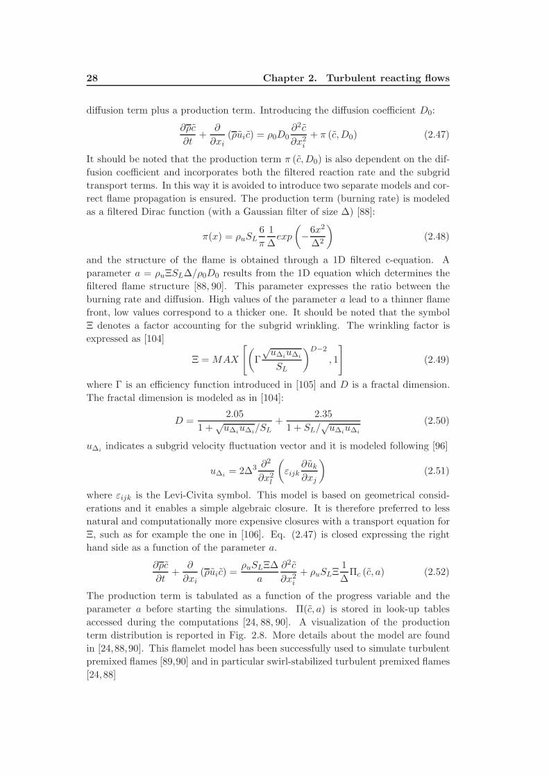
The production term is tabulated as a function of the progress variable and the
parameter a before starting the simulations. Π(c, a) is stored in look-up tables
accessed during the computations [24, 88, 90]. A visualization of the production
term distribution is reported in Fig. 2.8. More details about the model are found
in [24,88,90]. This flamelet model has been successfully used to simulate turbulent
premixed flames [89,90] and in particular swirl-stabilized turbulent premixed flames
[24,88]
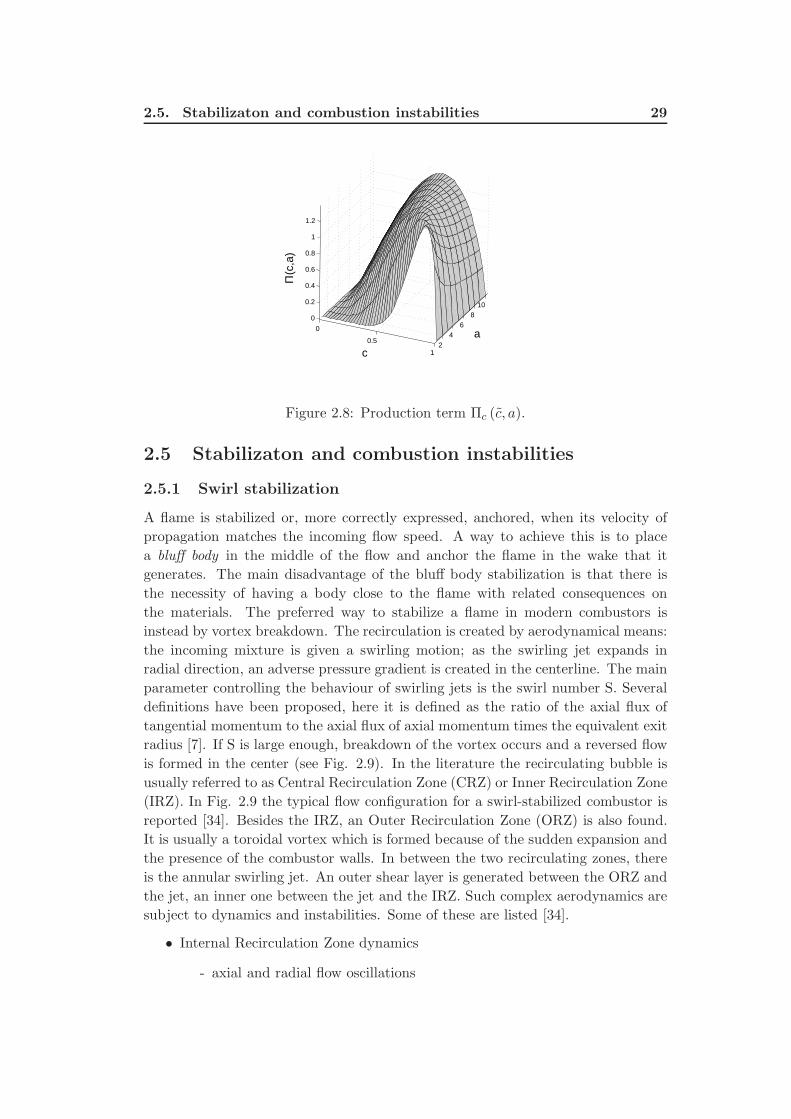
2.5. Stabilizaton and combustion instabilities 29
0
0.5
12
46
810
0
0.2
0.4
0.6
0.8
1
1.2
a
c
Π(c
,a)
Figure 2.8: Production term Πc (c, a).
2.5 Stabilizaton and combustion instabilities
2.5.1 Swirl stabilization
A flame is stabilized or, more correctly expressed, anchored, when its velocity of
propagation matches the incoming flow speed. A way to achieve this is to place
a bluff body in the middle of the flow and anchor the flame in the wake that it
generates. The main disadvantage of the bluff body stabilization is that there is
the necessity of having a body close to the flame with related consequences on
the materials. The preferred way to stabilize a flame in modern combustors is
instead by vortex breakdown. The recirculation is created by aerodynamical means:
the incoming mixture is given a swirling motion; as the swirling jet expands in
radial direction, an adverse pressure gradient is created in the centerline. The main
parameter controlling the behaviour of swirling jets is the swirl number S. Several
definitions have been proposed, here it is defined as the ratio of the axial flux of
tangential momentum to the axial flux of axial momentum times the equivalent exit
radius [7]. If S is large enough, breakdown of the vortex occurs and a reversed flow
is formed in the center (see Fig. 2.9). In the literature the recirculating bubble is
usually referred to as Central Recirculation Zone (CRZ) or Inner Recirculation Zone
(IRZ). In Fig. 2.9 the typical flow configuration for a swirl-stabilized combustor is
reported [34]. Besides the IRZ, an Outer Recirculation Zone (ORZ) is also found.
It is usually a toroidal vortex which is formed because of the sudden expansion and
the presence of the combustor walls. In between the two recirculating zones, there
is the annular swirling jet. An outer shear layer is generated between the ORZ and
the jet, an inner one between the jet and the IRZ. Such complex aerodynamics are
subject to dynamics and instabilities. Some of these are listed [34].
• Internal Recirculation Zone dynamics
- axial and radial flow oscillations
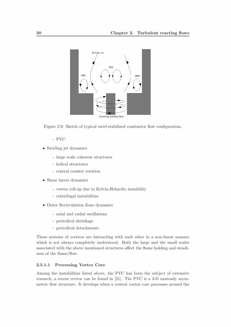
30 Chapter 2. Turbulent reacting flows
Figure 2.9: Sketch of typical swirl-stabilized combustor flow configuration.
- PVC
• Swirling jet dynamics
- large scale coherent structures
- helical structures
- central counter rotation
• Shear layers dynamics
- vortex roll-up due to Kelvin-Helmoltz instability
- centrifugal instabilities
• Outer Recirculation Zone dynamics
- axial and radial oscillations
- periodical shrinkage
- periodical detachments
These systems of vortices are interacting with each other in a non-linear manner
which is not always completely understood. Both the large and the small scales
associated with the above mentioned structures affect the flame holding and steadi-
ness of the flame/flow.
2.5.1.1 Precessing Vortex Core
Among the instabilities listed above, the PVC has been the subject of extensive
research; a recent review can be found in [21]. The PVC is a 3-D unsteady asym-
metric flow structure. It develops when a central vortex core precesses around the
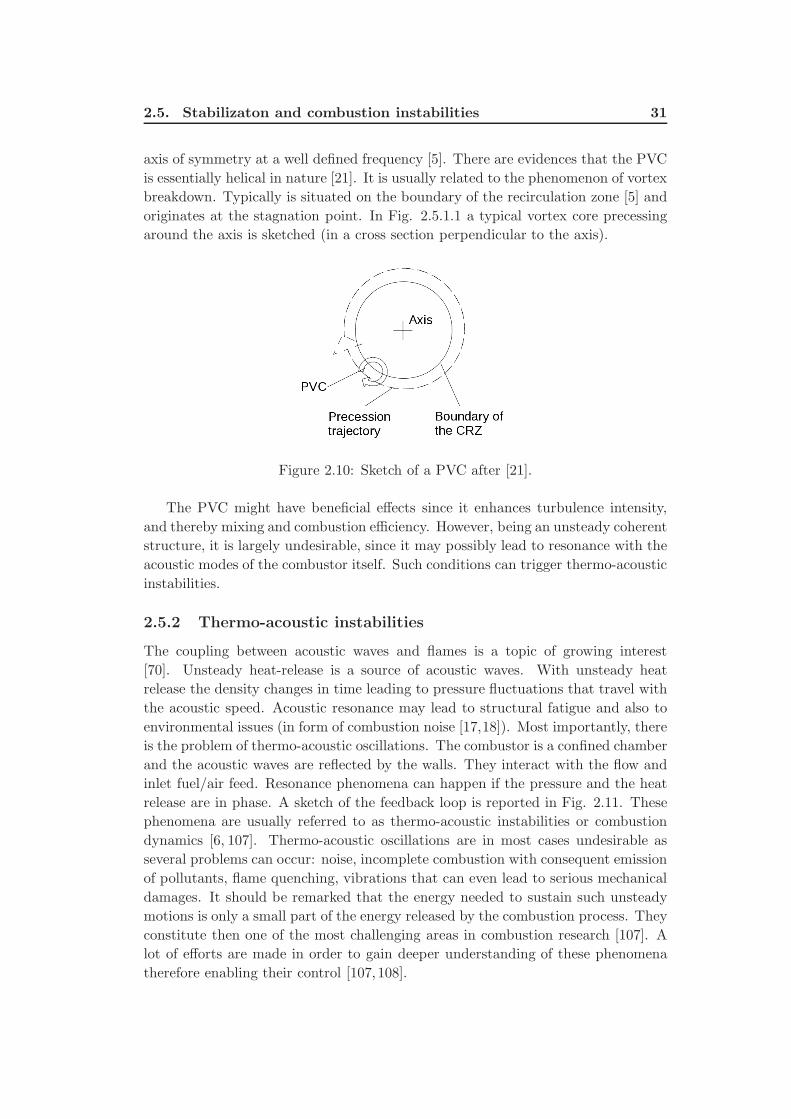
2.5. Stabilizaton and combustion instabilities 31
axis of symmetry at a well defined frequency [5]. There are evidences that the PVC
is essentially helical in nature [21]. It is usually related to the phenomenon of vortex
breakdown. Typically is situated on the boundary of the recirculation zone [5] and
originates at the stagnation point. In Fig. 2.5.1.1 a typical vortex core precessing
around the axis is sketched (in a cross section perpendicular to the axis).
Figure 2.10: Sketch of a PVC after [21].
The PVC might have beneficial effects since it enhances turbulence intensity,
and thereby mixing and combustion efficiency. However, being an unsteady coherent
structure, it is largely undesirable, since it may possibly lead to resonance with the
acoustic modes of the combustor itself. Such conditions can trigger thermo-acoustic
instabilities.
2.5.2 Thermo-acoustic instabilities
The coupling between acoustic waves and flames is a topic of growing interest
[70]. Unsteady heat-release is a source of acoustic waves. With unsteady heat
release the density changes in time leading to pressure fluctuations that travel with
the acoustic speed. Acoustic resonance may lead to structural fatigue and also to
environmental issues (in form of combustion noise [17,18]). Most importantly, there
is the problem of thermo-acoustic oscillations. The combustor is a confined chamber
and the acoustic waves are reflected by the walls. They interact with the flow and
inlet fuel/air feed. Resonance phenomena can happen if the pressure and the heat
release are in phase. A sketch of the feedback loop is reported in Fig. 2.11. These
phenomena are usually referred to as thermo-acoustic instabilities or combustion
dynamics [6, 107]. Thermo-acoustic oscillations are in most cases undesirable as
several problems can occur: noise, incomplete combustion with consequent emission
of pollutants, flame quenching, vibrations that can even lead to serious mechanical
damages. It should be remarked that the energy needed to sustain such unsteady
motions is only a small part of the energy released by the combustion process. They
constitute then one of the most challenging areas in combustion research [107]. A
lot of efforts are made in order to gain deeper understanding of these phenomena
therefore enabling their control [107,108].
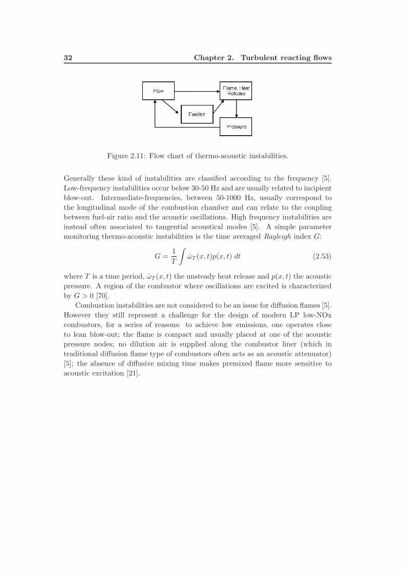
32 Chapter 2. Turbulent reacting flows
Figure 2.11: Flow chart of thermo-acoustic instabilities.
Generally these kind of instabilities are classified according to the frequency [5].
Low-frequency instabilities occur below 30-50 Hz and are usually related to incipient
blow-out. Intermediate-frequencies, between 50-1000 Hz, usually correspond to
the longitudinal mode of the combustion chamber and can relate to the coupling
between fuel-air ratio and the acoustic oscillations. High frequency instabilities are
instead often associated to tangential acoustical modes [5]. A simple parameter
monitoring thermo-acoustic instabilities is the time averaged Rayleigh index G:
G =1
T
∫ωT (x, t)p(x, t) dt (2.53)
where T is a time period, ωT (x, t) the unsteady heat release and p(x, t) the acoustic
pressure. A region of the combustor where oscillations are excited is characterized
by G > 0 [70].
Combustion instabilities are not considered to be an issue for diffusion flames [5].
However they still represent a challenge for the design of modern LP low-NOx
combustors, for a series of reasons: to achieve low emissions, one operates close
to lean blow-out; the flame is compact and usually placed at one of the acoustic
pressure nodes; no dilution air is supplied along the combustor liner (which in
traditional diffusion flame type of combustors often acts as an acoustic attenuator)
[5]; the absence of diffusive mixing time makes premixed flame more sensitive to
acoustic excitation [21].
Chapter 3
Methods
3.1 Numerical methods
The Navier-Stokes set of equations (Eq. 2.17-2.20) is a mathematical model to
describe the motion of fluids. It is a system of non-linear Partial Differential Equa-
tions (PDE). Analytical solutions are only possible if simplifying assumptions are
made (for example, two dimensional potential flow). For the full 3-D set of time-
dependent equations, a possibility is to get a numerical solution with the help of
computers. The field of numerical methods applied to fluid dynamics is generally
called Computational Fluid Dynamics (CFD). The equations are discretized into
an algebraic system of equations which can be solved on computers [109]. They
are solved on a discrete set of points in space, comprising a grid or mesh. Time
is also discretized. Most often, the three common discretization methods are the
Finite Difference (FD), the Finite Volume (FV) and the Finite Elements. These
three discretizations are related since they use polynomials for approximating the
continuous variables. A common approach for low Re computations on simple ge-
ometries is based on spectral approximations instead of polynomial ones, leading to
a higher accuracy with given number of degrees of freedom. However, for most CFD
applications polynomial based approaches are used to be able to handle non-trivial
geometries. FD methods are popular in academy because of their simplicity and
superior accuracy. A limitation is that complex geometries are difficult to handle.
In this thesis, the FD approach was used in the simulation of the Lisbon burner
(Paper I). An In-house code [110] was used for this scope. In contrast, FV meth-
ods, although at the price of accuracy loss, are suitable for complex geometries.
Therefore we used a FV approach for the simulations of the TARS burner (Papers
III,V,VI). Most commercial codes make use of FV Methods. We chose the Open
Source CFD tool box OpenFOAM [111, 112]. It is a rather complete CFD library
including both incompressible and compressible, non reacting and reacting solvers,
and a wide range of models. One can access the source code, and possibly mod-
ify it according to one’s own needs. In the following sections some details on the
discretization methods and the softwares used in this thesis are briefly introduced.
3.1.1 Finite Difference
In the Finite Difference method, the variables and their discrete derivatives are
stored at the grid points. The finite difference method enables to easily implement
high-order accurate schemes. This is due to the fact that finite differences are
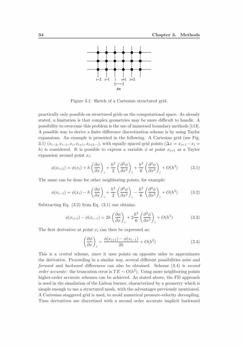
34 Chapter 3. Methods
Figure 3.1: Sketch of a Cartesian structured grid.
practically only possible on structured grids on the computational space. As already
stated, a limitation is that complex geometries may be more difficult to handle. A
possibility to overcome this problem is the use of immersed boundary methods [113].
A possible way to derive a finite difference discretization scheme is by using Taylor
expansions. An example is presented in the following. A Cartesian grid (see Fig.
3.1) (xi−2, xi−1, xi, xi+1, xi+2...), with equally spaced grid points (∆x = xi+1−xi =h) is considered. It is possible to express a variable φ at point xi+1 as a Taylor
expansion around point xi:
φ(xi+1) = φ(xi) + h
(∂φ
∂x
)
i
+h2
2
(∂2φ
∂x2
)
i
+h3
6
(∂3φ
∂x3
)
i
+O(h4) (3.1)
The same can be done for other neighboring points, for example:
φ(xi−1) = φ(xi)− h(∂φ
∂x
)
i
+h2
2
(∂2φ
∂x2
)
i
− h3
6
(∂3φ
∂x3
)
i
+O(h4) (3.2)
Subtracting Eq. (3.2) from Eq. (3.1) one obtains:
φ(xi+1)− φ(xi−1) = 2h
(∂φ
∂x
)
i
+ 2h3
6
(∂3φ
∂x3
)
i
+O(h5) (3.3)
The first derivative at point xi can then be expressed as:
(∂φ
∂x
)
i
=φ(xi+1)− φ(xi−1)
2h+O(h2) (3.4)
This is a central scheme, since it uses points on opposite sides to approximate
the derivative. Proceeding in a similar way, several different possibilities arise and
forward and backward differences can also be obtained. Scheme (3.4) is second
order accurate: the truncation error is TE ∼ O(h2). Using more neighboring points
higher-order accurate schemes can be achieved. As stated above, the FD approach
is used in the simulation of the Lisbon burner, characterized by a geometry which is
simple enough to use a structured mesh, with the advantages previously mentioned.
A Cartesian staggered grid is used, to avoid numerical pressure-velocity decoupling.
Time derivatives are discretized with a second order accurate implicit backward
3.1. Numerical methods 35
scheme. The diffusive terms are discretized with a fourth order central scheme,
while for the convective terms a fifth-order WENO scheme is adopted. The high-
order accuracy of the WENO scheme ensures low numerical dissipation. Moreover,
it is suitable to capture the steep gradients at the flame front. The different schemes
are briefly described in the following.
• Second order time derivative scheme
The time derivative of a generic variable φ is dicretized in the following way:
[110] (∂φ
∂t
)n+1
j
=3φn+1
j − 4φnj + φn−1j
2∆t(3.5)
where ∆t is the time step, the indices j and n refer to space and time, respec-
tively. The scheme is implicit: the derivative at the new time n+1 is depends
also on the value of variable φ at time n+ 1.
• Fourth order central scheme
Being h the mesh size, this scheme has the following expression [109]:
(∂2φ
∂x2
)
j
=−φj+2 + 16φj+1 − 30φj + 16φj−1 − φj−2
12h2+O(h4) (3.6)
• Fifth-order Weighted Essentially Non Oscillatory (WENO) scheme
The basic idea of the WENO [114] scheme is that instead of using one fixed
stencil to approximate the derivatives, several candidate stencils are consid-
ered. In the following its implementation is briefly described. For simplicity
a one-dimensional problem, the scalar conservation law, is considered:
ut + L(u) = ut + f(u)x = 0 (3.7)
To approximate the derivatives at xj the spatial operator L uses the fluxes
values f at half cell:
L =1
∆x
(fj+1/2 − fj−1/2
)(3.8)
where the hat indicates the discrete representation of the fluxes. The stencil
in WENO schemes is not fixed but adaptive. Using a number r of candidate
stencils, an order of accuracy of 2r− 1 is achieved. For a fifth-order accurate
scheme then r = 3 and the three candidate stencils reported in Fig. 3.2 are
considered to interpolate the fluxes. The interpolation schemes on the three
stencils respectively have the following expressions [114]:
f(1)j+1/2 =
1
3fj−2 −
7
6fj−1 +
11
6fj (3.9)
f(2)j+1/2 = −1
6fj−1 +
5
6fj +
1
3fj+1 (3.10)
f(3)j+1/2 =
1
3fj +
5
6fj+1 −
1
6fj+2 (3.11)
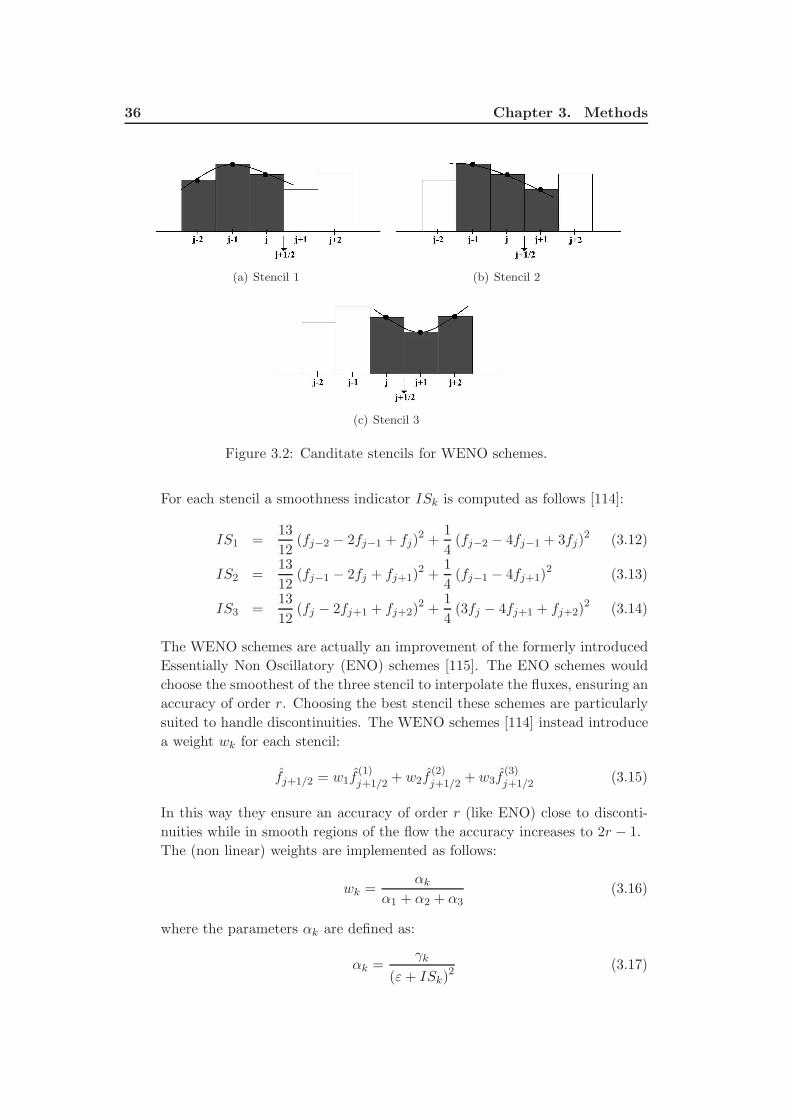
36 Chapter 3. Methods
(a) Stencil 1 (b) Stencil 2
(c) Stencil 3
Figure 3.2: Canditate stencils for WENO schemes.
For each stencil a smoothness indicator ISk is computed as follows [114]:
IS1 =13
12(fj−2 − 2fj−1 + fj)
2 +1
4(fj−2 − 4fj−1 + 3fj)
2 (3.12)
IS2 =13
12(fj−1 − 2fj + fj+1)
2 +1
4(fj−1 − 4fj+1)
2 (3.13)
IS3 =13
12(fj − 2fj+1 + fj+2)
2 +1
4(3fj − 4fj+1 + fj+2)
2 (3.14)
The WENO schemes are actually an improvement of the formerly introduced
Essentially Non Oscillatory (ENO) schemes [115]. The ENO schemes would
choose the smoothest of the three stencil to interpolate the fluxes, ensuring an
accuracy of order r. Choosing the best stencil these schemes are particularly
suited to handle discontinuities. The WENO schemes [114] instead introduce
a weight wk for each stencil:
fj+1/2 = w1f(1)j+1/2 + w2f
(2)j+1/2 + w3f
(3)j+1/2 (3.15)
In this way they ensure an accuracy of order r (like ENO) close to disconti-
nuities while in smooth regions of the flow the accuracy increases to 2r − 1.
The (non linear) weights are implemented as follows:
wk =αk
α1 + α2 + α3(3.16)
where the parameters αk are defined as:
αk =γk
(ε+ ISk)2 (3.17)
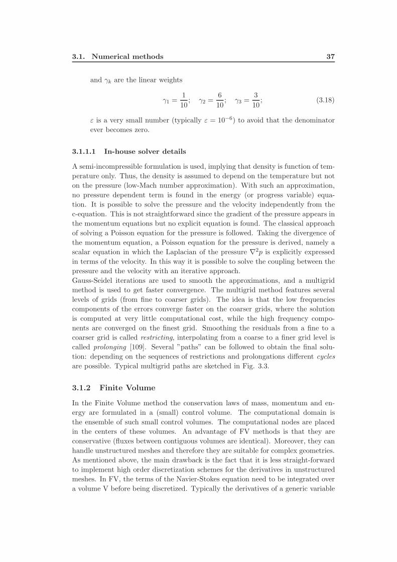
3.1. Numerical methods 37
and γk are the linear weights
γ1 =1
10; γ2 =
6
10; γ3 =
3
10; (3.18)
ε is a very small number (typically ε = 10−6) to avoid that the denominator
ever becomes zero.
3.1.1.1 In-house solver details
A semi-incompressible formulation is used, implying that density is function of tem-
perature only. Thus, the density is assumed to depend on the temperature but not
on the pressure (low-Mach number approximation). With such an approximation,
no pressure dependent term is found in the energy (or progress variable) equa-
tion. It is possible to solve the pressure and the velocity independently from the
c-equation. This is not straightforward since the gradient of the pressure appears in
the momentum equations but no explicit equation is found. The classical approach
of solving a Poisson equation for the pressure is followed. Taking the divergence of
the momentum equation, a Poisson equation for the pressure is derived, namely a
scalar equation in which the Laplacian of the pressure ∇2p is explicitly expressed
in terms of the velocity. In this way it is possible to solve the coupling between the
pressure and the velocity with an iterative approach.
Gauss-Seidel iterations are used to smooth the approximations, and a multigrid
method is used to get faster convergence. The multigrid method features several
levels of grids (from fine to coarser grids). The idea is that the low frequencies
components of the errors converge faster on the coarser grids, where the solution
is computed at very little computational cost, while the high frequency compo-
nents are converged on the finest grid. Smoothing the residuals from a fine to a
coarser grid is called restricting, interpolating from a coarse to a finer grid level is
called prolonging [109]. Several ”paths” can be followed to obtain the final solu-
tion: depending on the sequences of restrictions and prolongations different cycles
are possible. Typical multigrid paths are sketched in Fig. 3.3.
3.1.2 Finite Volume
In the Finite Volume method the conservation laws of mass, momentum and en-
ergy are formulated in a (small) control volume. The computational domain is
the ensemble of such small control volumes. The computational nodes are placed
in the centers of these volumes. An advantage of FV methods is that they are
conservative (fluxes between contiguous volumes are identical). Moreover, they can
handle unstructured meshes and therefore they are suitable for complex geometries.
As mentioned above, the main drawback is the fact that it is less straight-forward
to implement high order discretization schemes for the derivatives in unstructured
meshes. In FV, the terms of the Navier-Stokes equation need to be integrated over
a volume V before being discretized. Typically the derivatives of a generic variable
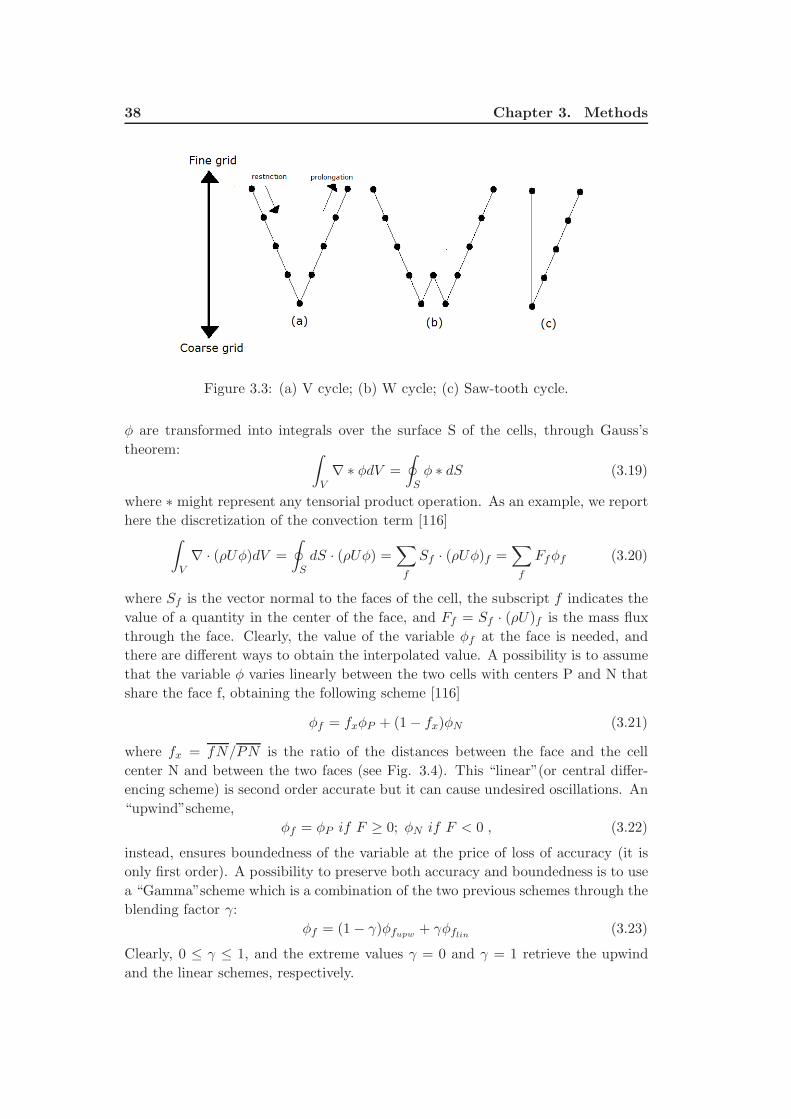
38 Chapter 3. Methods
Figure 3.3: (a) V cycle; (b) W cycle; (c) Saw-tooth cycle.
φ are transformed into integrals over the surface S of the cells, through Gauss’s
theorem: ∫
V∇ ∗ φdV =
∮
Sφ ∗ dS (3.19)
where ∗ might represent any tensorial product operation. As an example, we report
here the discretization of the convection term [116]∫
V∇ · (ρUφ)dV =
∮
SdS · (ρUφ) =
∑
f
Sf · (ρUφ)f =∑
f
Ffφf (3.20)
where Sf is the vector normal to the faces of the cell, the subscript f indicates the
value of a quantity in the center of the face, and Ff = Sf · (ρU)f is the mass flux
through the face. Clearly, the value of the variable φf at the face is needed, and
there are different ways to obtain the interpolated value. A possibility is to assume
that the variable φ varies linearly between the two cells with centers P and N that
share the face f, obtaining the following scheme [116]
φf = fxφP + (1− fx)φN (3.21)
where fx = fN/PN is the ratio of the distances between the face and the cell
center N and between the two faces (see Fig. 3.4). This “linear”(or central differ-
encing scheme) is second order accurate but it can cause undesired oscillations. An
“upwind”scheme,
φf = φP if F ≥ 0; φN if F < 0 , (3.22)
instead, ensures boundedness of the variable at the price of loss of accuracy (it is
only first order). A possibility to preserve both accuracy and boundedness is to use
a “Gamma”scheme which is a combination of the two previous schemes through the
blending factor γ:
φf = (1− γ)φfupw + γφflin (3.23)
Clearly, 0 ≤ γ ≤ 1, and the extreme values γ = 0 and γ = 1 retrieve the upwind
and the linear schemes, respectively.
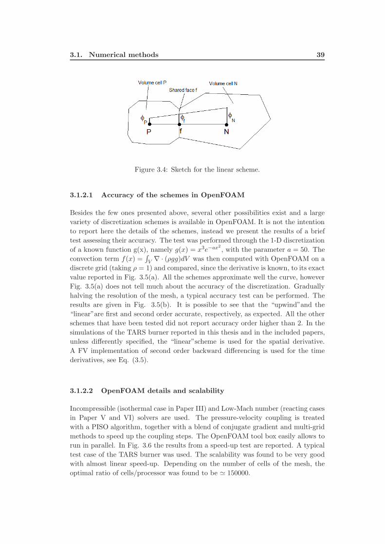
3.1. Numerical methods 39
Figure 3.4: Sketch for the linear scheme.
3.1.2.1 Accuracy of the schemes in OpenFOAM
Besides the few ones presented above, several other possibilities exist and a large
variety of discretization schemes is available in OpenFOAM. It is not the intention
to report here the details of the schemes, instead we present the results of a brief
test assessing their accuracy. The test was performed through the 1-D discretization
of a known function g(x), namely g(x) = x3e−ax2
, with the parameter a = 50. The
convection term f(x) =∫V ∇ · (ρgg)dV was then computed with OpenFOAM on a
discrete grid (taking ρ = 1) and compared, since the derivative is known, to its exact
value reported in Fig. 3.5(a). All the schemes approximate well the curve, however
Fig. 3.5(a) does not tell much about the accuracy of the discretization. Gradually
halving the resolution of the mesh, a typical accuracy test can be performed. The
results are given in Fig. 3.5(b). It is possible to see that the “upwind”and the
“linear”are first and second order accurate, respectively, as expected. All the other
schemes that have been tested did not report accuracy order higher than 2. In the
simulations of the TARS burner reported in this thesis and in the included papers,
unless differently specified, the “linear”scheme is used for the spatial derivative.
A FV implementation of second order backward differencing is used for the time
derivatives, see Eq. (3.5).
3.1.2.2 OpenFOAM details and scalability
Incompressible (isothermal case in Paper III) and Low-Mach number (reacting cases
in Paper V and VI) solvers are used. The pressure-velocity coupling is treated
with a PISO algorithm, together with a blend of conjugate gradient and multi-grid
methods to speed up the coupling steps. The OpenFOAM tool box easily allows to
run in parallel. In Fig. 3.6 the results from a speed-up test are reported. A typical
test case of the TARS burner was used. The scalability was found to be very good
with almost linear speed-up. Depending on the number of cells of the mesh, the
optimal ratio of cells/processor was found to be ≃ 150000.
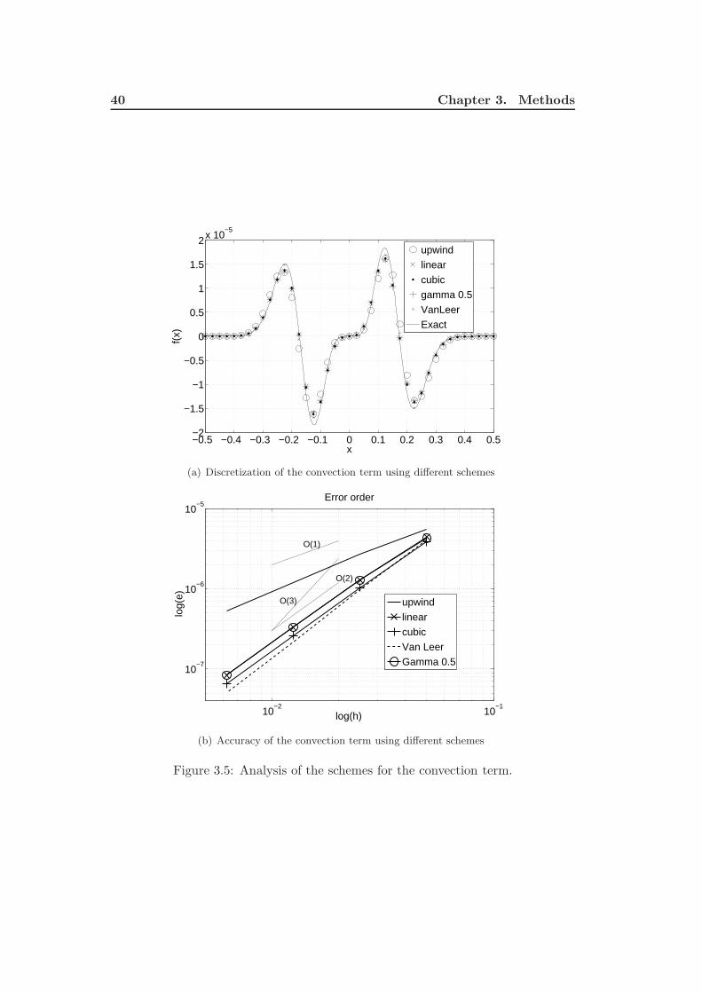
40 Chapter 3. Methods
−0.5 −0.4 −0.3 −0.2 −0.1 0 0.1 0.2 0.3 0.4 0.5−2
−1.5
−1
−0.5
0
0.5
1
1.5
2x 10⁻⁵
x
f(x)
upwind
linear
cubic
gamma 0.5
VanLeer
Exact
(a) Discretization of the convection term using different schemes
10−2
10−1
10−7
10−6
10−5
log(h)
log(
e)
Error order
upwind
linear
cubic
Van Leer
Gamma 0.5
O(3)
O(2)
O(1)
(b) Accuracy of the convection term using different schemes
Figure 3.5: Analysis of the schemes for the convection term.
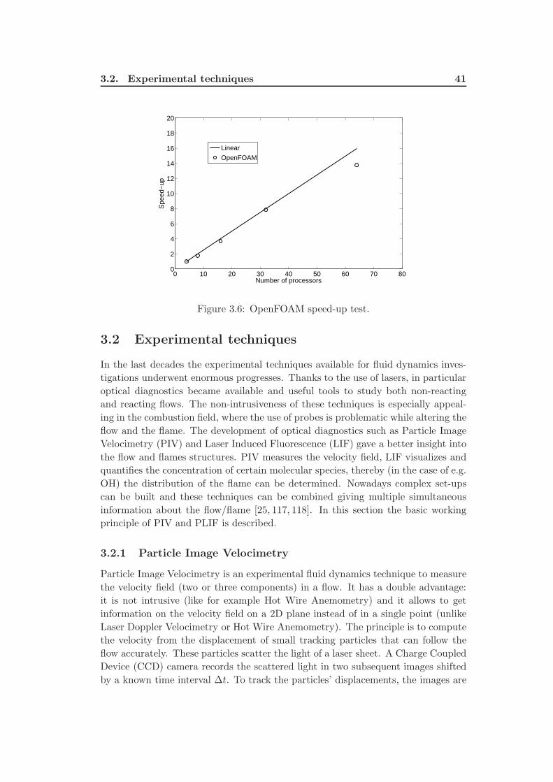
3.2. Experimental techniques 41
0 10 20 30 40 50 60 70 800
2
4
6
8
10
12
14
16
18
20
Number of processors
Spe
ed−
up
Linear
OpenFOAM
Figure 3.6: OpenFOAM speed-up test.
3.2 Experimental techniques
In the last decades the experimental techniques available for fluid dynamics inves-
tigations underwent enormous progresses. Thanks to the use of lasers, in particular
optical diagnostics became available and useful tools to study both non-reacting
and reacting flows. The non-intrusiveness of these techniques is especially appeal-
ing in the combustion field, where the use of probes is problematic while altering the
flow and the flame. The development of optical diagnostics such as Particle Image
Velocimetry (PIV) and Laser Induced Fluorescence (LIF) gave a better insight into
the flow and flames structures. PIV measures the velocity field, LIF visualizes and
quantifies the concentration of certain molecular species, thereby (in the case of e.g.
OH) the distribution of the flame can be determined. Nowadays complex set-ups
can be built and these techniques can be combined giving multiple simultaneous
information about the flow/flame [25, 117, 118]. In this section the basic working
principle of PIV and PLIF is described.
3.2.1 Particle Image Velocimetry
Particle Image Velocimetry is an experimental fluid dynamics technique to measure
the velocity field (two or three components) in a flow. It has a double advantage:
it is not intrusive (like for example Hot Wire Anemometry) and it allows to get
information on the velocity field on a 2D plane instead of in a single point (unlike
Laser Doppler Velocimetry or Hot Wire Anemometry). The principle is to compute
the velocity from the displacement of small tracking particles that can follow the
flow accurately. These particles scatter the light of a laser sheet. A Charge Coupled
Device (CCD) camera records the scattered light in two subsequent images shifted
by a known time interval ∆t. To track the particles’ displacements, the images are
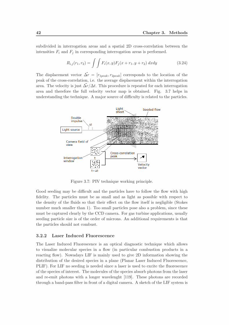
42 Chapter 3. Methods
subdivided in interrogation areas and a spatial 2D cross-correlation between the
intensities Fi and Fj in corresponding interrogation areas is performed.
Ri,j(r1, r2) =
∫ ∫Fi(x, y)Fj(x+ r1, y + r2) dxdy (3.24)
The displacement vector ~∆r = [r1peak, r2peak] corresponds to the location of the
peak of the cross-correlation, i.e. the average displacement within the interrogation
area. The velocity is just ~∆r/∆t. This procedure is repeated for each interrogation
area and therefore the full velocity vector map is obtained. Fig. 3.7 helps in
understanding the technique. A major source of difficulty is related to the particles.
Figure 3.7: PIV technique working principle.
Good seeding may be difficult and the particles have to follow the flow with high
fidelity. The particles must be as small and as light as possible with respect to
the density of the fluids so that their effect on the flow itself is negligible (Stokes
number much smaller than 1). Too small particles pose also a problem, since these
must be captured clearly by the CCD camera. For gas turbine applications, usually
seeding particle size is of the order of microns. An additional requirements is that
the particles should not combust.
3.2.2 Laser Induced Fluorescence
The Laser Induced Fluorescence is an optical diagnostic technique which allows
to visualize molecular species in a flow (in particular combustion products in a
reacting flow). Nowadays LIF is mainly used to give 2D information showing the
distribution of the desired species in a plane (Planar Laser Induced Fluorescence,
PLIF). For LIF no seeding is needed since a laser is used to excite the fluorescence
of the species of interest. The molecules of the species absorb photons from the laser
and re-emit photons with a longer wavelenght [119]. These photons are recorded
through a band-pass filter in front of a digital camera. A sketch of the LIF system is
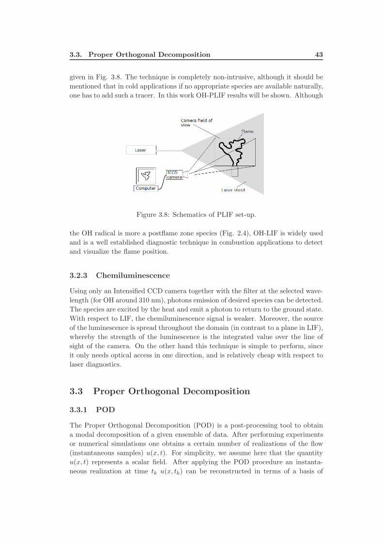
3.3. Proper Orthogonal Decomposition 43
given in Fig. 3.8. The technique is completely non-intrusive, although it should be
mentioned that in cold applications if no appropriate species are available naturally,
one has to add such a tracer. In this work OH-PLIF results will be shown. Although
Figure 3.8: Schematics of PLIF set-up.
the OH radical is more a postflame zone species (Fig. 2.4), OH-LIF is widely used
and is a well established diagnostic technique in combustion applications to detect
and visualize the flame position.
3.2.3 Chemiluminescence
Using only an Intensified CCD camera together with the filter at the selected wave-
length (for OH around 310 nm), photons emission of desired species can be detected.
The species are excited by the heat and emit a photon to return to the ground state.
With respect to LIF, the chemiluminescence signal is weaker. Moreover, the source
of the luminescence is spread throughout the domain (in contrast to a plane in LIF),
whereby the strength of the luminescence is the integrated value over the line of
sight of the camera. On the other hand this technique is simple to perform, since
it only needs optical access in one direction, and is relatively cheap with respect to
laser diagnostics.
3.3 Proper Orthogonal Decomposition
3.3.1 POD
The Proper Orthogonal Decomposition (POD) is a post-processing tool to obtain
a modal decomposition of a given ensemble of data. After performing experiments
or numerical simulations one obtains a certain number of realizations of the flow
(instantaneous samples) u(x, t). For simplicity, we assume here that the quantity
u(x, t) represents a scalar field. After applying the POD procedure an instanta-
neous realization at time tk u(x, tk) can be reconstructed in terms of a basis of
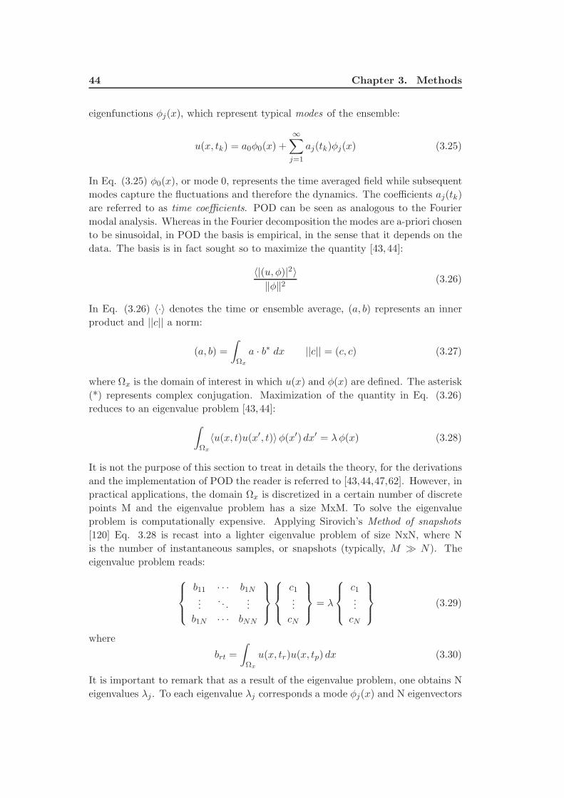
44 Chapter 3. Methods
eigenfunctions φj(x), which represent typical modes of the ensemble:
u(x, tk) = a0φ0(x) +∞∑
j=1
aj(tk)φj(x) (3.25)
In Eq. (3.25) φ0(x), or mode 0, represents the time averaged field while subsequent
modes capture the fluctuations and therefore the dynamics. The coefficients aj(tk)
are referred to as time coefficients. POD can be seen as analogous to the Fourier
modal analysis. Whereas in the Fourier decomposition the modes are a-priori chosen
to be sinusoidal, in POD the basis is empirical, in the sense that it depends on the
data. The basis is in fact sought so to maximize the quantity [43,44]:
〈|(u, φ)|2〉‖φ‖2 (3.26)
In Eq. (3.26) 〈·〉 denotes the time or ensemble average, (a, b) represents an inner
product and ||c|| a norm:
(a, b) =
∫
Ωx
a · b∗ dx ||c|| = (c, c) (3.27)
where Ωx is the domain of interest in which u(x) and φ(x) are defined. The asterisk
(*) represents complex conjugation. Maximization of the quantity in Eq. (3.26)
reduces to an eigenvalue problem [43,44]:
∫
Ωx
〈u(x, t)u(x′, t)〉φ(x′) dx′ = λφ(x) (3.28)
It is not the purpose of this section to treat in details the theory, for the derivations
and the implementation of POD the reader is referred to [43,44,47,62]. However, in
practical applications, the domain Ωx is discretized in a certain number of discrete
points M and the eigenvalue problem has a size MxM. To solve the eigenvalue
problem is computationally expensive. Applying Sirovich’s Method of snapshots
[120] Eq. 3.28 is recast into a lighter eigenvalue problem of size NxN, where N
is the number of instantaneous samples, or snapshots (typically, M ≫ N). The
eigenvalue problem reads:
b11 · · · b1N...
. . ....
b1N · · · bNN
c1...
cN
= λ
c1...
cN
(3.29)
where
brt =
∫
Ωx
u(x, tr)u(x, tp) dx (3.30)
It is important to remark that as a result of the eigenvalue problem, one obtains N
eigenvalues λj . To each eigenvalue λj corresponds a mode φj(x) and N eigenvectors
3.3. Proper Orthogonal Decomposition 45
cj(tk). In the method of snapshots the modes are expressed as a linear combination
of the instantaneous realizations:
φj(x) =1
λjN
N∑
k=1
cj(tk)u(x, tk) (3.31)
The eigenvalues are ordered in descending order λj > λj+1 and represent the en-
ergetic content of the modes. Thus, if the variable u to which the decomposition
is applied represents the velocity, the first POD modes have the highest turbulent
kinetic energy content and typically identify coherent structures. The time coeffi-
cients in Eq. (3.25) are computed projecting the modes on the snapshots. The time
coefficient relative to the j-th mode and the k-th instantaneous sample reads:
aj(tk) = φj(x) · u(x, tk) (3.32)
3.3.2 Extended POD
The main idea behind Extended-POD (EPOD) is to see how events are correlated
in space or time. One considers a second realization α(x, t) which is obtained
simultaneously to u(x, t). For example, α(x, t) might represent another variable
like pressure, temperature, species concentration, progress variable, or even the
same variable u on a different domain. The idea is then to project the second data
set on the eigenvectors of the original POD analysis. In this way the procedure
”distillates” the part of the signal of the variable α which is correlated to the POD
modes of the original variable of analysis u. The extended modes ψj(x) are defined
as [58,59,62]:
ψj(x) =1
λjN
N∑
k=1
cj(tk)α(x, tk) (3.33)
In other words statistical quantities conditioned to the dominant fluctuations of
u are generated. Conditioned variables have been a key tool for understanding
fluctuations in flames. EPOD extends the idea by linking any unsteady variable
(OH concentration, progress variable) with statistical quantities describing the large
scale fluctuations of the field u (velocity in this case).
In the papers presented in this thesis, EPOD is applied to realizations in which
the variable α is representative of the flame (progress variable for the numerical
simulations, Paper I [61], OH-signal for experimental data, Paper II, [62] ). In this
way it is possible to highlight the correlations between flow and flame dynamics.
This procedure is therefore very helpful to investigate combustion dynamics. For
more details on theory and implementation, the reader is referred to [58,59,62].
3.3.3 Time coefficients information and interlink with phase aver-aging
A “very special property” [121] of the Proper Orthogonal Decomposition is the
spatio-temporal relation between the modes and the instantaneous samples through
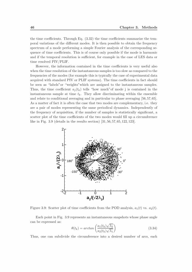
46 Chapter 3. Methods
the time coefficients. Through Eq. (3.32) the time coefficients summarize the tem-
poral variations of the different modes. It is then possible to obtain the frequency
spectrum of a mode performing a simple Fourier analysis of the corresponding se-
quence of time coefficients. This is of course only possible if the mode is harmonic
and if the temporal resolution is sufficient, for example in the case of LES data or
time resolved PIV/PLIF.
However, the information contained in the time coefficients is very useful also
when the time resolution of the instantaneous samples is too slow as compared to the
frequencies of the modes (for example this is typically the case of experimental data
acquired with standard PIV or PLIF systems). The time coefficients in fact should
be seen as “labels”or “weights”which are assigned to the instantaneous samples.
Thus, the time coefficient aj(tk) tells “how much”of mode j is contained in the
instantaneous sample at time tk. They allow discriminating within the ensemble
and relate to conditional averaging and in particular to phase averaging [56,57,65].
As a matter of fact it is often the case that two modes are complementary, i.e. they
are a pair of modes representing the same periodical dynamics. Independently of
the frequency of acquisition, if the number of samples is statistically significant, a
scatter plot of the time coefficients of the two modes would fill up a circumference
like in Fig. 3.9 (details in the results section) [31,56,57,65,122,123].
a2/(√2λ2)
a 1/√(
2λ 1
)
-2 -1 0 1 2-2
-1
0
1
2
0o
300
-30o
180o
-150o
Figure 3.9: Scatter plot of time coefficients from the POD analysis, a1(t) vs. a2(t).
Each point in Fig. 3.9 represents an instantaneous snapshots whose phase angle
can be expressed as:
θ(tk) = arctan
(a1(tk)
√λ2
a2(tk)√λ1
)(3.34)
Thus, one can subdivide the circumference into a desired number of arcs, each

3.3. Proper Orthogonal Decomposition 47
sector corresponding to a given phase-angle. With this information, it is possible
to perform an a-posteriori phase average of the original instantaneous snapshots
ensemble. No additional information (phase-locking, simultaneous pressure signal)
is needed beside the ensemble of independent and randomly acquired samples.

Chapter 4
Problem Set-up
In this thesis, two academic research burners are studied: the Lisbon and the TARS
combustors. In this chapter, their geometrical features will be detailed. For the
cases investigated, the operating conditions, the experimental and numerical set-
ups will be given. Brief overview of previous studies will also be presented. The
Lisbon burner, given its simplicity, is believed to be a good test-case to investigate
the dynamics of swirling flames and in particular the response of vortex break-
down/flame stabilization to axial oscillations. The TARS fuel-injector combines
laboratory flexibility and complex geometry, similar to a real aero-engine design.
In this work it is investigated both numerically and experimentally. The analysis
is challenging given the multi-scale physics and the complexity of the flow and the
flame.
4.1 Lisbon burner
A sketch of the Lisbon combustor [23] is shown in Fig. 4.1. Following the flow from
left to the right, the combustor is composed by:
• Swirl generator: It features adjustable blade angles to set the desired swirl
number.
• Converging annulus: Connecting the swirler to the premixing tube.
• Premixing tube: A premixing pipe of 0.05 m diameter ensures a mixture
with the fuel which is injected at the exit of a bluff body downstream the
swirl generator.
• Throat The premixing tube is connected to the combustion chamber through
a converging diverging nozzle with minimum diameter equal D=0.04 m.
• Combustion chamber The combustion chamber is axysymmetric and has
a diameter of 0.11m. It is 0.336 m long.
This model combustor was experimentally studied at Lisbon Technical University
mainly using LDV, flow visualization techniques, pressure probes, and gas temper-
ature sampling [20, 23, 42, 60]. Both reacting and non-reacting flows revealed the
existence of helical structures and PVC for high enough swirl numbers. This com-
bustor has also been numerically computed by means of LES [24]. The simulations
successfully reproduced the experimental data and with the help of Proper Orthog-
onal Decomposition highlighted the structures found in the experiments. The PVC
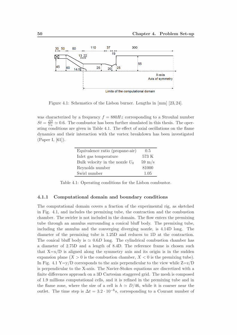
50 Chapter 4. Problem Set-up
Figure 4.1: Schematics of the Lisbon burner. Lengths in [mm] [23,24].
was characterized by a frequency f = 880Hz corresponding to a Strouhal number
St = fDU0≃ 0.6. The combustor has been further simulated in this thesis. The oper-
ating conditions are given in Table 4.1. The effect of axial oscillations on the flame
dynamics and their interaction with the vortex breakdown has been investigated
(Paper I, [61]).
Equivalence ratio (propane-air) 0.5
Inlet gas temperature 573 K
Bulk velocity in the nozzle U0 59 m/s
Reynolds number 81000
Swirl number 1.05
Table 4.1: Operating conditions for the Lisbon combustor.
4.1.1 Computational domain and boundary conditions
The computational domain covers a fraction of the experimental rig, as sketched
in Fig. 4.1, and includes the premixing tube, the contraction and the combustion
chamber. The swirler is not included in the domain. The flow enters the premixing
tube through an annulus surrounding a conical bluff body. The premixing tube,
including the annulus and the converging diverging nozzle, is 4.14D long. The
diameter of the premixing tube is 1.25D and reduces to 1D at the contraction.
The conical bluff body is ≃ 0.6D long. The cylindrical combustion chamber has
a diameter of 2.75D and a length of 8.4D. The reference frame is chosen such
that X=x/D is aligned along the symmetry axis and its origin is in the sudden
expansion plane (X > 0 is the combustion chamber, X < 0 is the premixing tube).
In Fig. 4.1 Y=y/D corresponds to the axis perpendicular to the view while Z=z/D
is perpendicular to the X-axis. The Navier-Stokes equations are discretized with a
finite differences approach on a 3D Cartesian staggered grid. The mesh is composed
of 1.9 millions computational cells, and it is refined in the premixing tube and in
the flame zone, where the size of a cell is h ≃ D/46, while it is coarser near the
outlet. The time step is ∆t = 3.2 · 10−6s, corresponding to a Courant number of
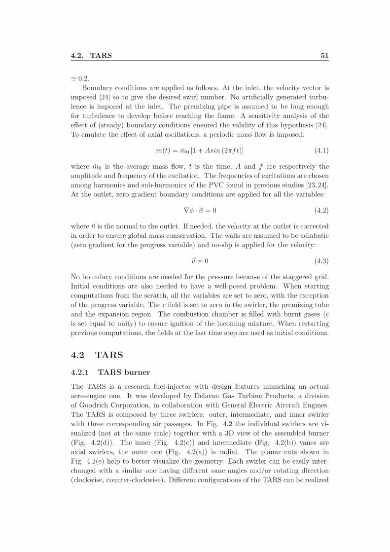
4.2. TARS 51
≃ 0.2.
Boundary conditions are applied as follows. At the inlet, the velocity vector is
imposed [24] so to give the desired swirl number. No artificially generated turbu-
lence is imposed at the inlet. The premixing pipe is assumed to be long enough
for turbulence to develop before reaching the flame. A sensitivity analysis of the
effect of (steady) boundary conditions ensured the validity of this hypothesis [24].
To emulate the effect of axial oscillations, a periodic mass flow is imposed:
m(t) = m0 [1 +Asin (2πft)] (4.1)
where m0 is the average mass flow, t is the time, A and f are respectively the
amplitude and frequency of the excitation. The frequencies of excitations are chosen
among harmonics and sub-harmonics of the PVC found in previous studies [23,24].
At the outlet, zero gradient boundary conditions are applied for all the variables:
∇φ · ~n = 0 (4.2)
where ~n is the normal to the outlet. If needed, the velocity at the outlet is corrected
in order to ensure global mass conservation. The walls are assumed to be adiabatic
(zero gradient for the progress variable) and no-slip is applied for the velocity:
~v = 0 (4.3)
No boundary conditions are needed for the pressure because of the staggered grid.
Initial conditions are also needed to have a well-posed problem. When starting
computations from the scratch, all the variables are set to zero, with the exception
of the progress variable. The c field is set to zero in the swirler, the premixing tube
and the expansion region. The combustion chamber is filled with burnt gases (c
is set equal to unity) to ensure ignition of the incoming mixture. When restarting
previous computations, the fields at the last time step are used as initial conditions.
4.2 TARS
4.2.1 TARS burner
The TARS is a research fuel-injector with design features mimicking an actual
aero-engine one. It was developed by Delavan Gas Turbine Products, a division
of Goodrich Corporation, in collaboration with General Electric Aircraft Engines.
The TARS is composed by three swirlers: outer, intermediate, and inner swirler
with three corresponding air passages. In Fig. 4.2 the individual swirlers are vi-
sualized (not at the same scale) together with a 3D view of the assembled burner
(Fig. 4.2(d)). The inner (Fig. 4.2(c)) and intermediate (Fig. 4.2(b)) vanes are
axial swirlers, the outer one (Fig. 4.2(a)) is radial. The planar cuts shown in
Fig. 4.2(e) help to better visualize the geometry. Each swirler can be easily inter-
changed with a similar one having different vane angles and/or rotating direction
(clockwise, counter-clockwise). Different configurations of the TARS can be realized
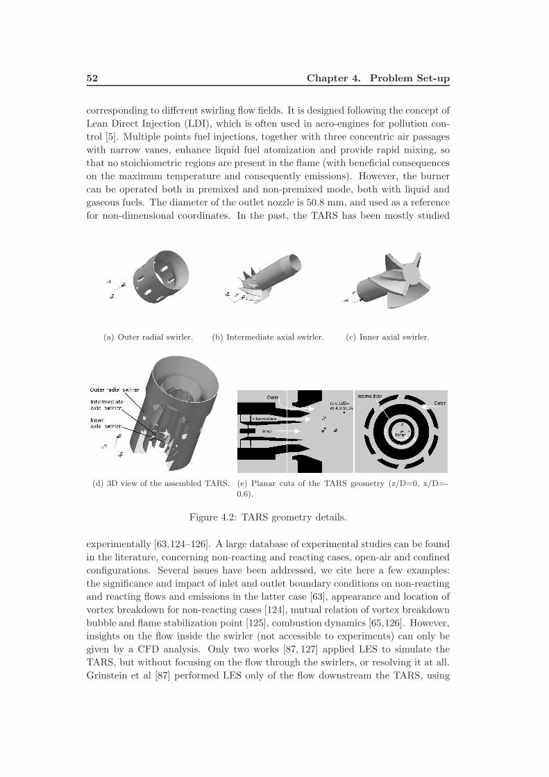
52 Chapter 4. Problem Set-up
corresponding to different swirling flow fields. It is designed following the concept of
Lean Direct Injection (LDI), which is often used in aero-engines for pollution con-
trol [5]. Multiple points fuel injections, together with three concentric air passages
with narrow vanes, enhance liquid fuel atomization and provide rapid mixing, so
that no stoichiometric regions are present in the flame (with beneficial consequences
on the maximum temperature and consequently emissions). However, the burner
can be operated both in premixed and non-premixed mode, both with liquid and
gaseous fuels. The diameter of the outlet nozzle is 50.8 mm, and used as a reference
for non-dimensional coordinates. In the past, the TARS has been mostly studied
(a) Outer radial swirler. (b) Intermediate axial swirler. (c) Inner axial swirler.
(d) 3D view of the assembled TARS. (e) Planar cuts of the TARS geometry (z/D=0, x/D=-
0.6).
Figure 4.2: TARS geometry details.
experimentally [63,124–126]. A large database of experimental studies can be found
in the literature, concerning non-reacting and reacting cases, open-air and confined
configurations. Several issues have been addressed, we cite here a few examples:
the significance and impact of inlet and outlet boundary conditions on non-reacting
and reacting flows and emissions in the latter case [63], appearance and location of
vortex breakdown for non-reacting cases [124], mutual relation of vortex breakdown
bubble and flame stabilization point [125], combustion dynamics [65,126]. However,
insights on the flow inside the swirler (not accessible to experiments) can only be
given by a CFD analysis. Only two works [87, 127] applied LES to simulate the
TARS, but without focusing on the flow through the swirlers, or resolving it at all.
Grinstein et al [87] performed LES only of the flow downstream the TARS, using
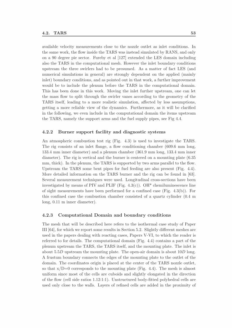
4.2. TARS 53
available velocity measurements close to the nozzle outlet as inlet conditions. In
the same work, the flow inside the TARS was instead simulated by RANS, and only
on a 90 degree pie sector. Fureby et al [127] extended the LES domain including
also the TARS in the computational mesh. However the inlet boundary conditions
upstream the three swirlers had to be presumed. As a matter of fact LES (and
numerical simulations in general) are strongly dependent on the applied (mainly
inlet) boundary conditions, and as pointed out in that work, a further improvement
would be to include the plenum before the TARS in the computational domain.
This has been done in this work. Moving the inlet further upstream, one can let
the mass flow to split through the swirler vanes according to the geometry of the
TARS itself, leading to a more realistic simulation, affected by less assumptions,
getting a more reliable view of the dynamics. Furthermore, as it will be clarified
in the following, we even include in the computational domain the items upstream
the TARS, namely the support arms and the fuel supply pipes, see Fig 4.4.
4.2.2 Burner support facility and diagnostic systems
An atmospheric combustion test rig (Fig. 4.3) is used to investigate the TARS.
The rig consists of an inlet flange, a flow conditioning chamber (609.6 mm long,
133.4 mm inner diameter) and a plenum chamber (361.9 mm long, 133.4 mm inner
diameter). The rig is vertical and the burner is centered on a mounting plate (6.35
mm, thick). In the plenum, the TARS is supported by two arms parallel to the flow.
Upstream the TARS some bent pipes for fuel feeding are also present (Fig. 4.4).
More detailed information on the TARS burner and the rig can be found in [63].
Several measurement techniques were used. Longitudinal cross-sections have been
investigated by means of PIV and PLIF (Fig. 4.3(c)). OH* chemiluminescence line
of sight measurements have been performed for a confined case (Fig. 4.3(b)). For
this confined case the combustion chamber consisted of a quartz cylinder (0.4 m
long, 0.11 m inner diameter).
4.2.3 Computational Domain and boundary conditions
The mesh that will be described here refers to the isothermal case study of Paper
III [64], for which we report some results in Section 5.2. Slightly different meshes are
used in the papers dealing with reacting cases, Papers V-VI, to which the reader is
referred to for details. The computational domain (Fig. 4.4) contains a part of the
plenum upstream the TARS, the TARS itself, and the mounting plate. The inlet is
about 5.5D upstream the mounting plate. The open-air domain is about 10D long.
A frustum boundary connects the edges of the mounting plate to the outlet of the
domain. The coordinates origin is placed at the center of the TARS nozzle outlet,
so that x/D=0 corresponds to the mounting plate (Fig. 4.4). The mesh is almost
uniform since most of the cells are cuboids and slightly elongated in the direction
of the flow (cell side ratios 1.12:1:1). Unstructured body-fitted polyhedral cells are
used only close to the walls. Layers of refined cells are added in the proximity of
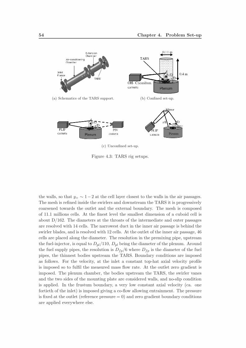
54 Chapter 4. Problem Set-up
(a) Schematics of the TARS support. (b) Confined set-up.
(c) Unconfined set-up.
Figure 4.3: TARS rig setups.
the walls, so that y+ ∼ 1−2 at the cell layer closest to the walls in the air passages.
The mesh is refined inside the swirlers and downstream the TARS it is progressively
coarsened towards the outlet and the external boundary. The mesh is composed
of 11.1 millions cells. At the finest level the smallest dimension of a cuboid cell is
about D/162. The diameters at the throats of the intermediate and outer passages
are resolved with 14 cells. The narrowest duct in the inner air passage is behind the
swirler blades, and is resolved with 12 cells. At the outlet of the inner air passage, 46
cells are placed along the diameter. The resolution in the premixing pipe, upstream
the fuel-injector, is equal toDpl/110, Dpl being the diameter of the plenum. Around
the fuel supply pipes, the resolution is Dfp/6 where Dfp is the diameter of the fuel
pipes, the thinnest bodies upstream the TARS. Boundary conditions are imposed
as follows. For the velocity, at the inlet a constant top-hat axial velocity profile
is imposed so to fulfil the measured mass flow rate. At the outlet zero gradient is
imposed. The plenum chamber, the bodies upstream the TARS, the swirler vanes
and the two sides of the mounting plate are considered walls, and no-slip condition
is applied. In the frustum boundary, a very low constant axial velocity (ca. one
fortieth of the inlet) is imposed giving a co-flow allowing entrainment. The pressure
is fixed at the outlet (reference pressure = 0) and zero gradient boundary conditions
are applied everywhere else.
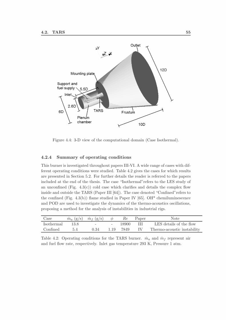
4.2. TARS 55
Figure 4.4: 3-D view of the computational domain (Case Isothermal).
4.2.4 Summary of operating conditions
This burner is investigated throughout papers III-VI. A wide range of cases with dif-
ferent operating conditions were studied. Table 4.2 gives the cases for which results
are presented in Section 5.2. For further details the reader is referred to the papers
included at the end of the thesis. The case “Isothermal”refers to the LES study of
an unconfined (Fig. 4.3(c)) cold case which clarifies and details the complex flow
inside and outside the TARS (Paper III [64]). The case denoted “Confined”refers to
the confined (Fig. 4.3(b)) flame studied in Paper IV [65]. OH* chemiluminescence
and POD are used to investigate the dynamics of the thermo-acoustics oscillations,
proposing a method for the analysis of instabilities in industrial rigs.
Case ma (g/s) mf (g/s) φ Re Paper Note
Isothermal 13.8 - - 18900 III LES details of the flow
Confined 5.4 0.34 1.19 7849 IV Thermo-acoustic instability
Table 4.2: Operating conditions for the TARS burner. ma and mf represent air
and fuel flow rate, respectively. Inlet gas temperature 293 K, Pressure 1 atm.

Chapter 5
Summary of results
In this chapter relevant exemplifying results are briefly summarized. For a more
detailed analysis and the complete set of problems and cases the reader is further
referred to the papers enclosed at the end of this thesis.
5.1 Lisbon burner
The works of [23,24] describe for this combustor the existence of a pair of counter-
rotating helical structures leading to a precessing vortex core. Such structures have
a characteristic frequency of 880 Hz, corresponding to a Strouhal number St = 0.6.
This section summarizes the effect of axial forcing at half the frequency of the PVC
(St = 0.3). The excitation is performed by means of sinusoidal fluctuations of the
inlet mass flow, see Eq. (4.1). The amplitude of the excitation is set to 20% of the
average mass flow.
5.1.1 Statistics
In Fig. 5.1 the average effect of the axial forcing is shown. The top frame shows
the unforced case while in the bottom frame the time averaged field for the forced
case is shown. The isolines describe the progress variable c (thus the flame). The
flow features the typical IRZ caused by vortex breakdown and the toroidal ORZ
between the walls and the expansion. The flame is located at the shear layers
between the recirculation zones but is decoupled from the recirculating bubble,
because of the PVC. As a global effect of the excitation, the flame is stabilized
further upstream in the forced case, and the IRZ is also pulled upstream on average.
Averaged quantitative profiles are shown in Fig. 5.2 quantifying a shifting in axial
stabilization point of ∆X ∼ 0.25.
5.1.2 POD analysis
When averaging with traditional statistics, all the information about the dynamics
is smoothed out. Therefore, POD is applied to characterize the most energetic
modes of the flow. The results of the POD analysis in a longitudinal section are
given in Fig. 5.3. Modes 1-4 for the forced case are shown. For each mode, the power
spectrum of the time coefficients sequence gives a characteristic frequency of the
mode itself. Modes 1 and 2 are a pair: they represent the same dynamics, namely
axial fluctuations in the premixing tube. They correspond to the imposed forcing
as confirmed by the peak at the same frequency as the excitation (St=0.3). Modes
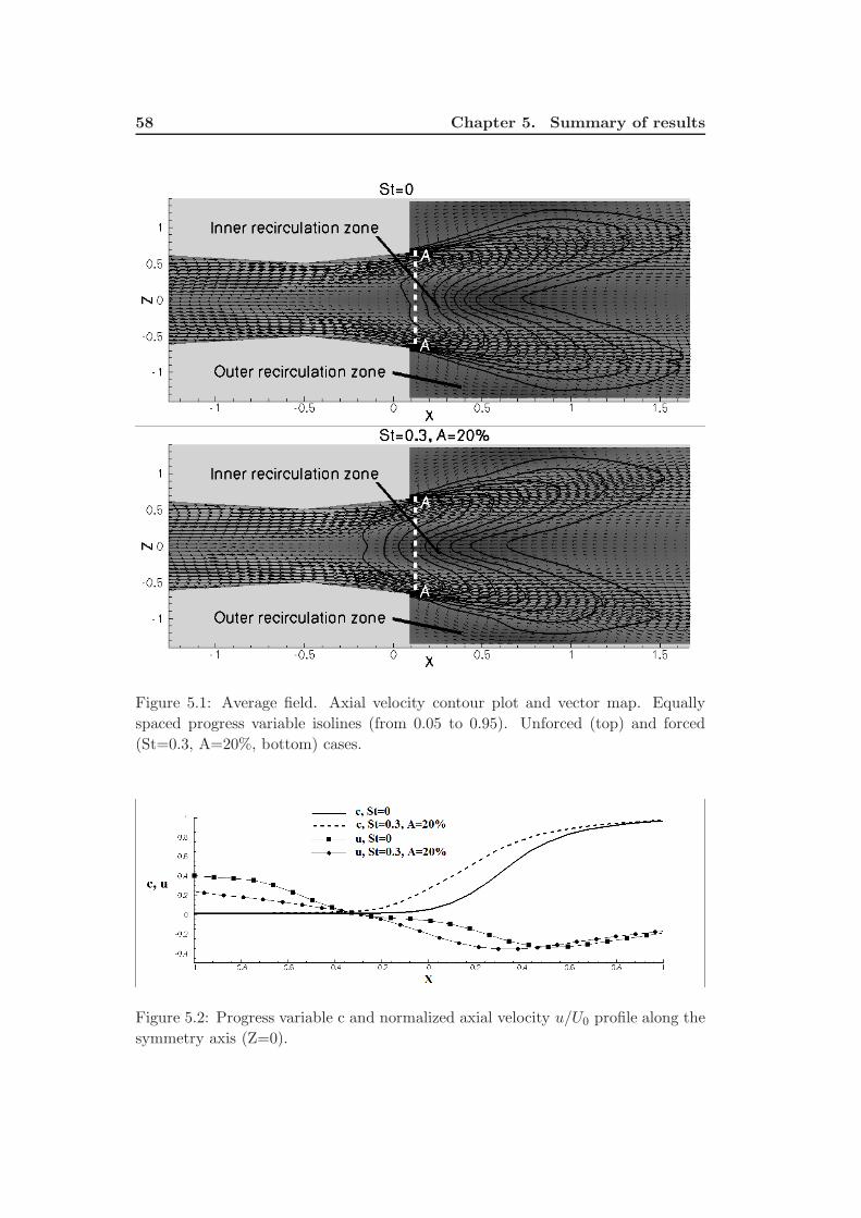
58 Chapter 5. Summary of results
Figure 5.1: Average field. Axial velocity contour plot and vector map. Equally
spaced progress variable isolines (from 0.05 to 0.95). Unforced (top) and forced
(St=0.3, A=20%, bottom) cases.
Figure 5.2: Progress variable c and normalized axial velocity u/U0 profile along the
symmetry axis (Z=0).
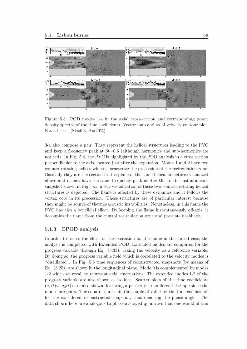
5.1. Lisbon burner 59
Figure 5.3: POD modes 1-4 in the axial cross-section and corresponding power
density spectra of the time coefficients. Vector map and axial velocity contour plot.
Forced case, (St=0.3, A=20%).
3-4 also compose a pair. They represent the helical structures leading to the PVC
and keep a frequency peak at St=0.6 (although harmonics and sub-harmonics are
noticed). In Fig. 5.4, the PVC is highlighted by the POD analysis in a cross section
perpendicular to the axis, located just after the expansion. Modes 1 and 2 have two
counter rotating helices which characterize the precession of the recirculation zone.
Basically they are the section in this plane of the same helical structures visualized
above and in fact have the same frequency peak at St=0.6. In the instantaneous
snapshot shown in Fig. 5.5, a 3-D visualization of these two counter-rotating helical
structures is depicted. The flame is affected by these dynamics and it follows the
vortex core in its precession. These structures are of particular interest because
they might be source of thermo-acoustic instabilities. Nonetheless, in this flame the
PVC has also a beneficial effect. By keeping the flame instantaneously off-axis, it
decouples the flame from the central recirculation zone and prevents flashback.
5.1.3 EPOD analysis
In order to assess the effect of the excitation on the flame in the forced case, the
analysis is completed with Extended POD. Extended modes are computed for the
progress variable through Eq. (3.33), taking the velocity as a reference variable.
By doing so, the progress variable field which is correlated to the velocity modes is
“distillated”. In Fig. 5.6 time sequences of reconstructed snapshots (by means of
Eq. (3.25)) are shown in the longitudinal plane. Mode 0 is complemented by modes
1-2 which we recall to represent axial fluctuations. The extended modes 1-2 of the
progress variable are also shown as isolines. Scatter plots of the time coefficients
(a1(t)vs a2(t)) are also shown, featuring a perfectly circumferential shape since the
modes are pairs. The square represents the couple of values of the time coefficients
for the considered reconstructed snapshot, thus denoting the phase angle. The
data shown here are analogous to phase-averaged quantities that one would obtain
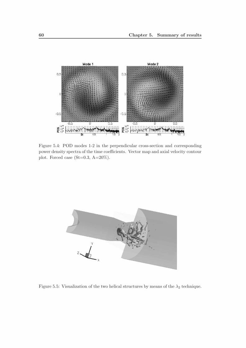
60 Chapter 5. Summary of results
Figure 5.4: POD modes 1-2 in the perpendicular cross-section and corresponding
power density spectra of the time coefficients. Vector map and axial velocity contour
plot. Forced case (St=0.3, A=20%).
Figure 5.5: Visualization of the two helical structures by means of the λ2 technique.
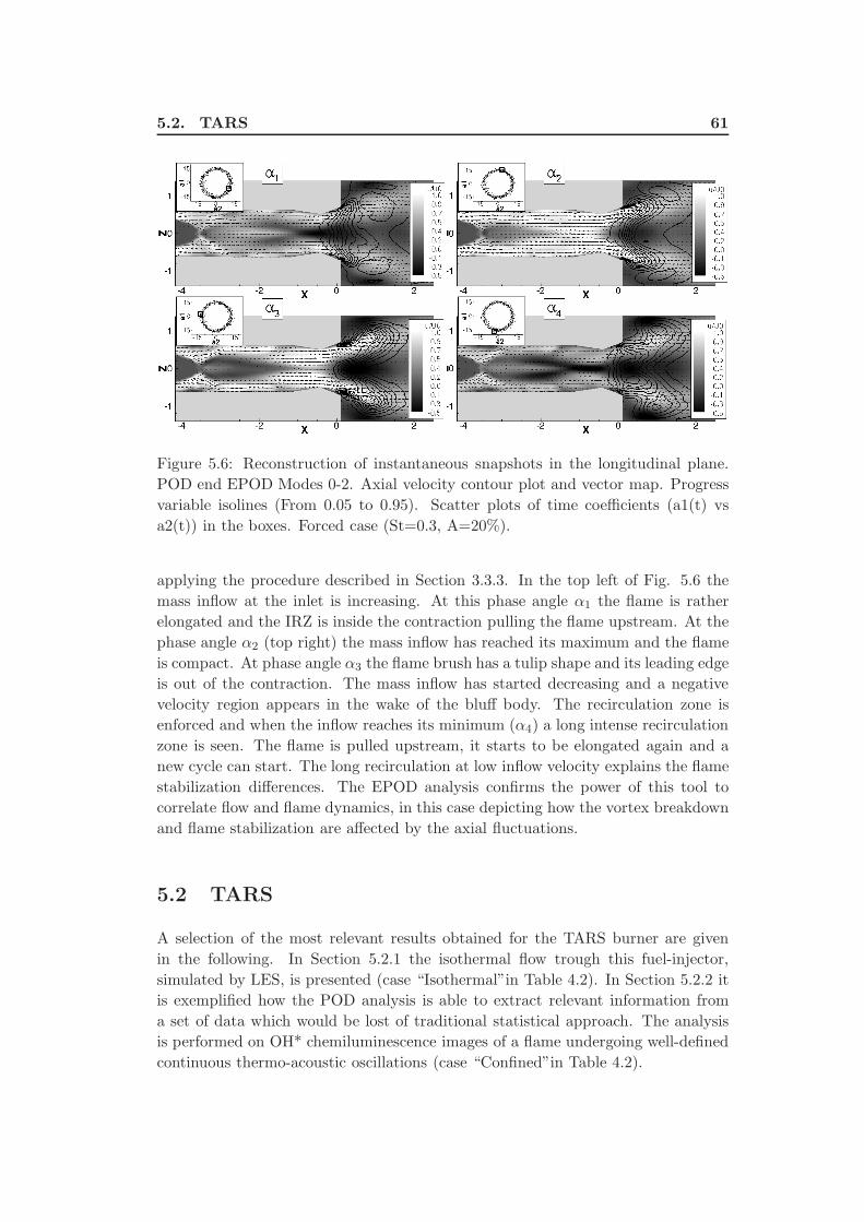
5.2. TARS 61
Figure 5.6: Reconstruction of instantaneous snapshots in the longitudinal plane.
POD end EPOD Modes 0-2. Axial velocity contour plot and vector map. Progress
variable isolines (From 0.05 to 0.95). Scatter plots of time coefficients (a1(t) vs
a2(t)) in the boxes. Forced case (St=0.3, A=20%).
applying the procedure described in Section 3.3.3. In the top left of Fig. 5.6 the
mass inflow at the inlet is increasing. At this phase angle α1 the flame is rather
elongated and the IRZ is inside the contraction pulling the flame upstream. At the
phase angle α2 (top right) the mass inflow has reached its maximum and the flame
is compact. At phase angle α3 the flame brush has a tulip shape and its leading edge
is out of the contraction. The mass inflow has started decreasing and a negative
velocity region appears in the wake of the bluff body. The recirculation zone is
enforced and when the inflow reaches its minimum (α4) a long intense recirculation
zone is seen. The flame is pulled upstream, it starts to be elongated again and a
new cycle can start. The long recirculation at low inflow velocity explains the flame
stabilization differences. The EPOD analysis confirms the power of this tool to
correlate flow and flame dynamics, in this case depicting how the vortex breakdown
and flame stabilization are affected by the axial fluctuations.
5.2 TARS
A selection of the most relevant results obtained for the TARS burner are given
in the following. In Section 5.2.1 the isothermal flow trough this fuel-injector,
simulated by LES, is presented (case “Isothermal”in Table 4.2). In Section 5.2.2 it
is exemplified how the POD analysis is able to extract relevant information from
a set of data which would be lost of traditional statistical approach. The analysis
is performed on OH* chemiluminescence images of a flame undergoing well-defined
continuous thermo-acoustic oscillations (case “Confined”in Table 4.2).
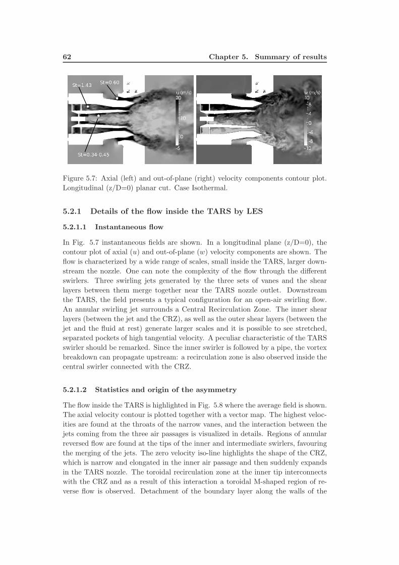
62 Chapter 5. Summary of results
Figure 5.7: Axial (left) and out-of-plane (right) velocity components contour plot.
Longitudinal (z/D=0) planar cut. Case Isothermal.
5.2.1 Details of the flow inside the TARS by LES
5.2.1.1 Instantaneous flow
In Fig. 5.7 instantaneous fields are shown. In a longitudinal plane (z/D=0), the
contour plot of axial (u) and out-of-plane (w) velocity components are shown. The
flow is characterized by a wide range of scales, small inside the TARS, larger down-
stream the nozzle. One can note the complexity of the flow through the different
swirlers. Three swirling jets generated by the three sets of vanes and the shear
layers between them merge together near the TARS nozzle outlet. Downstream
the TARS, the field presents a typical configuration for an open-air swirling flow.
An annular swirling jet surrounds a Central Recirculation Zone. The inner shear
layers (between the jet and the CRZ), as well as the outer shear layers (between the
jet and the fluid at rest) generate larger scales and it is possible to see stretched,
separated pockets of high tangential velocity. A peculiar characteristic of the TARS
swirler should be remarked. Since the inner swirler is followed by a pipe, the vortex
breakdown can propagate upstream: a recirculation zone is also observed inside the
central swirler connected with the CRZ.
5.2.1.2 Statistics and origin of the asymmetry
The flow inside the TARS is highlighted in Fig. 5.8 where the average field is shown.
The axial velocity contour is plotted together with a vector map. The highest veloc-
ities are found at the throats of the narrow vanes, and the interaction between the
jets coming from the three air passages is visualized in details. Regions of annular
reversed flow are found at the tips of the inner and intermediate swirlers, favouring
the merging of the jets. The zero velocity iso-line highlights the shape of the CRZ,
which is narrow and elongated in the inner air passage and then suddenly expands
in the TARS nozzle. The toroidal recirculation zone at the inner tip interconnects
with the CRZ and as a result of this interaction a toroidal M-shaped region of re-
verse flow is observed. Detachment of the boundary layer along the walls of the
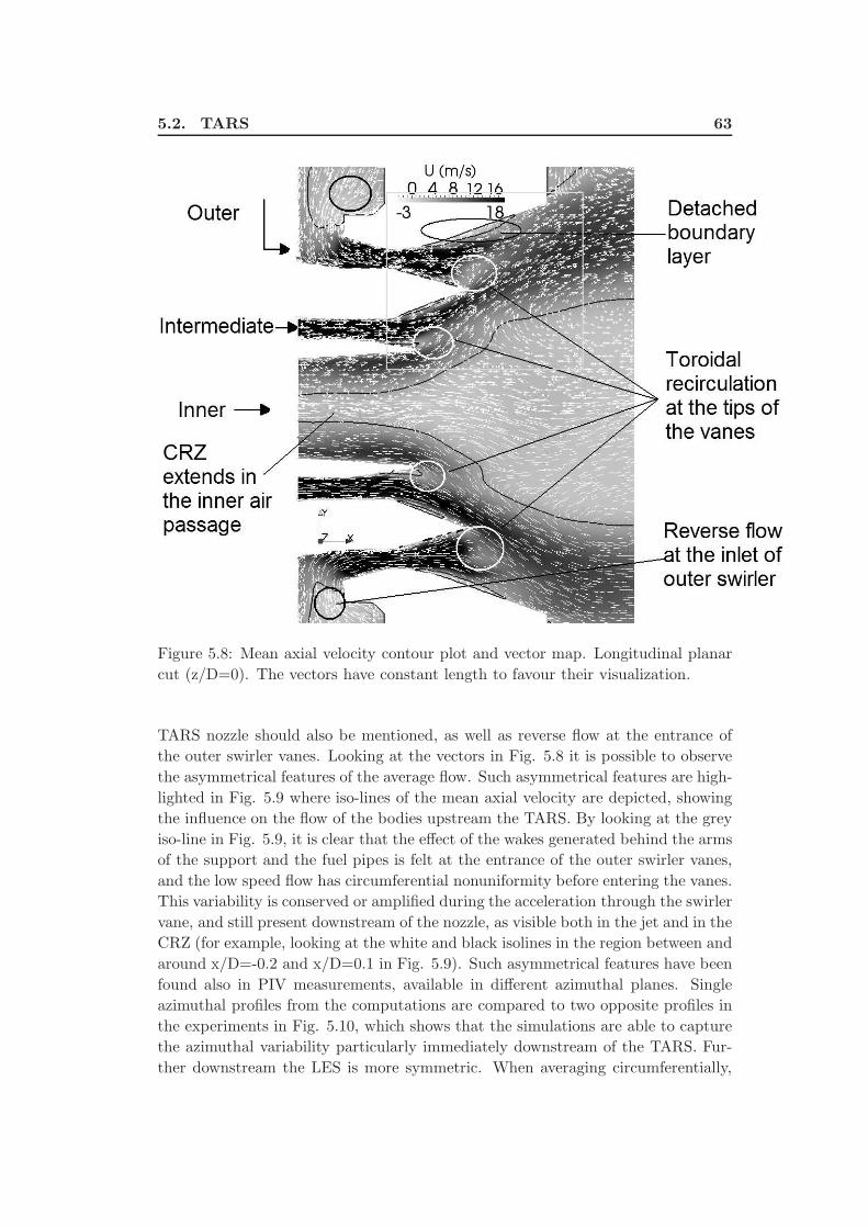
5.2. TARS 63
Figure 5.8: Mean axial velocity contour plot and vector map. Longitudinal planar
cut (z/D=0). The vectors have constant length to favour their visualization.
TARS nozzle should also be mentioned, as well as reverse flow at the entrance of
the outer swirler vanes. Looking at the vectors in Fig. 5.8 it is possible to observe
the asymmetrical features of the average flow. Such asymmetrical features are high-
lighted in Fig. 5.9 where iso-lines of the mean axial velocity are depicted, showing
the influence on the flow of the bodies upstream the TARS. By looking at the grey
iso-line in Fig. 5.9, it is clear that the effect of the wakes generated behind the arms
of the support and the fuel pipes is felt at the entrance of the outer swirler vanes,
and the low speed flow has circumferential nonuniformity before entering the vanes.
This variability is conserved or amplified during the acceleration through the swirler
vane, and still present downstream of the nozzle, as visible both in the jet and in the
CRZ (for example, looking at the white and black isolines in the region between and
around x/D=-0.2 and x/D=0.1 in Fig. 5.9). Such asymmetrical features have been
found also in PIV measurements, available in different azimuthal planes. Single
azimuthal profiles from the computations are compared to two opposite profiles in
the experiments in Fig. 5.10, which shows that the simulations are able to capture
the azimuthal variability particularly immediately downstream of the TARS. Fur-
ther downstream the LES is more symmetric. When averaging circumferentially,
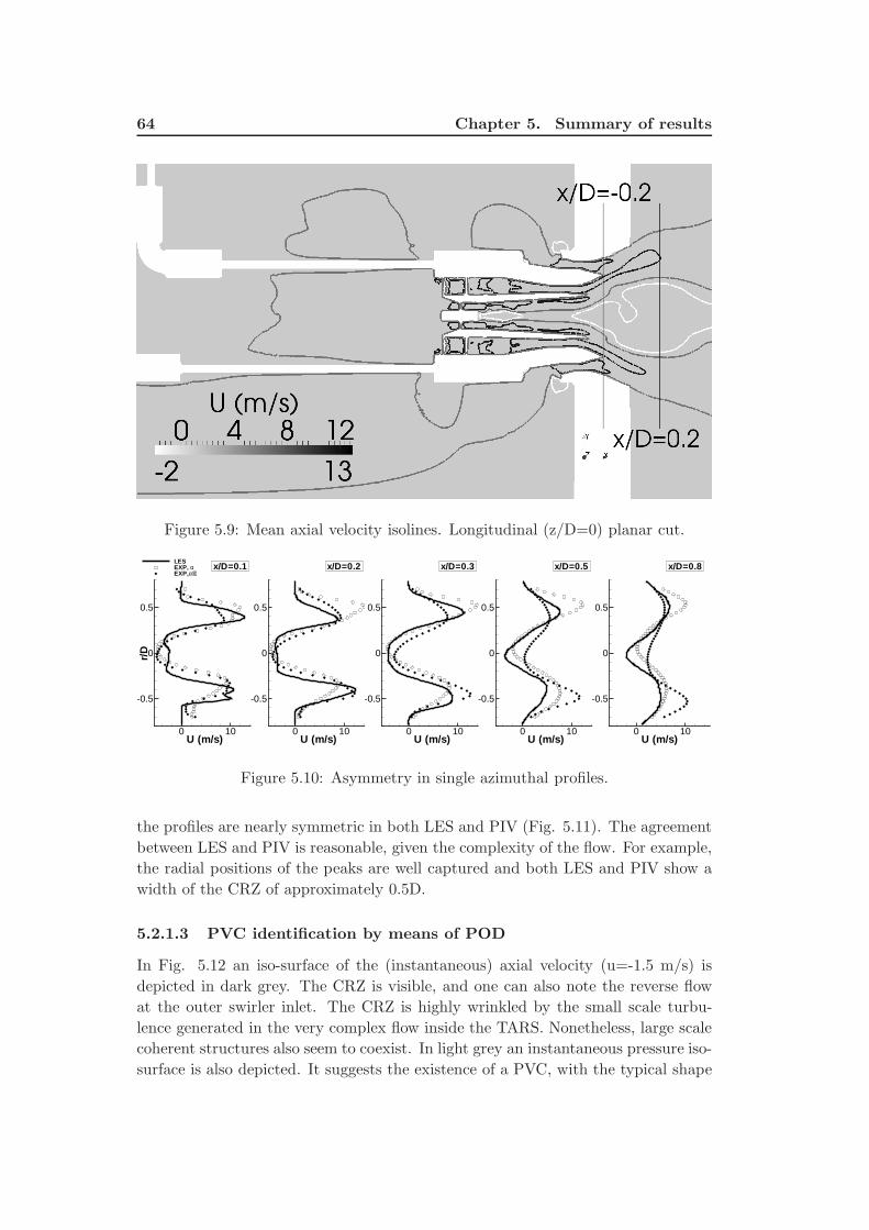
64 Chapter 5. Summary of results
Figure 5.9: Mean axial velocity isolines. Longitudinal (z/D=0) planar cut.
U (m/s)
r/D
0 10
-0.5
0
0.5
LESEXP, αEXP,α+π
x/D=0.1
U (m/s)0 10
-0.5
0
0.5
x/D=0.2
U (m/s)0 10
-0.5
0
0.5
x/D=0.3
U (m/s)0 10
-0.5
0
0.5
x/D=0.5
U (m/s)0 10
-0.5
0
0.5
x/D=0.8
Figure 5.10: Asymmetry in single azimuthal profiles.
the profiles are nearly symmetric in both LES and PIV (Fig. 5.11). The agreement
between LES and PIV is reasonable, given the complexity of the flow. For example,
the radial positions of the peaks are well captured and both LES and PIV show a
width of the CRZ of approximately 0.5D.
5.2.1.3 PVC identification by means of POD
In Fig. 5.12 an iso-surface of the (instantaneous) axial velocity (u=-1.5 m/s) is
depicted in dark grey. The CRZ is visible, and one can also note the reverse flow
at the outer swirler inlet. The CRZ is highly wrinkled by the small scale turbu-
lence generated in the very complex flow inside the TARS. Nonetheless, large scale
coherent structures also seem to coexist. In light grey an instantaneous pressure iso-
surface is also depicted. It suggests the existence of a PVC, with the typical shape
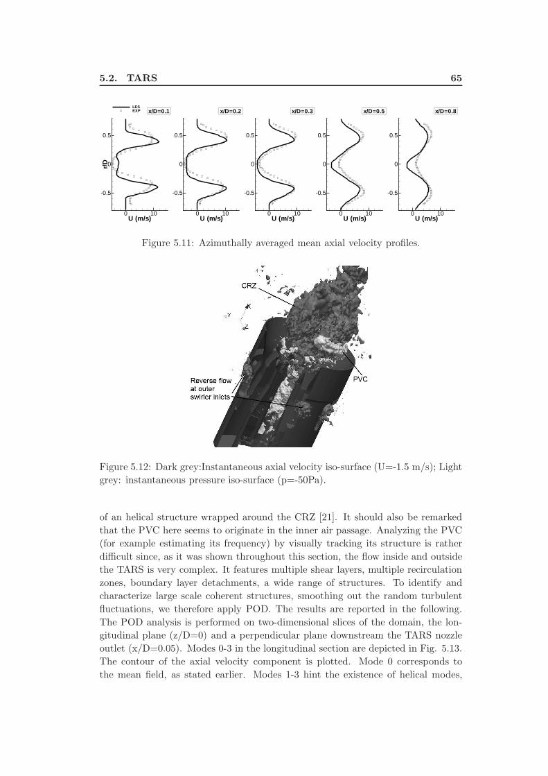
5.2. TARS 65
U (m/s)
r/D
0 10
-0.5
0
0.5
LESEXP x/D=0.1
U (m/s)0 10
-0.5
0
0.5
x/D=0.2
U (m/s)0 10
-0.5
0
0.5
x/D=0.3
U (m/s)0 10
-0.5
0
0.5
x/D=0.5
U (m/s)0 10
-0.5
0
0.5
x/D=0.8
Figure 5.11: Azimuthally averaged mean axial velocity profiles.
Figure 5.12: Dark grey:Instantaneous axial velocity iso-surface (U=-1.5 m/s); Light
grey: instantaneous pressure iso-surface (p=-50Pa).
of an helical structure wrapped around the CRZ [21]. It should also be remarked
that the PVC here seems to originate in the inner air passage. Analyzing the PVC
(for example estimating its frequency) by visually tracking its structure is rather
difficult since, as it was shown throughout this section, the flow inside and outside
the TARS is very complex. It features multiple shear layers, multiple recirculation
zones, boundary layer detachments, a wide range of structures. To identify and
characterize large scale coherent structures, smoothing out the random turbulent
fluctuations, we therefore apply POD. The results are reported in the following.
The POD analysis is performed on two-dimensional slices of the domain, the lon-
gitudinal plane (z/D=0) and a perpendicular plane downstream the TARS nozzle
outlet (x/D=0.05). Modes 0-3 in the longitudinal section are depicted in Fig. 5.13.
The contour of the axial velocity component is plotted. Mode 0 corresponds to
the mean field, as stated earlier. Modes 1-3 hint the existence of helical modes,
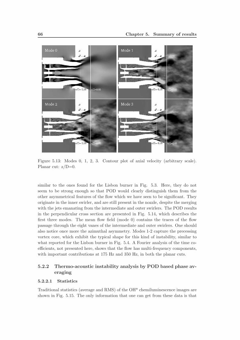
66 Chapter 5. Summary of results
Figure 5.13: Modes 0, 1, 2, 3. Contour plot of axial velocity (arbitrary scale).
Planar cut: z/D=0.
similar to the ones found for the Lisbon burner in Fig. 5.3. Here, they do not
seem to be strong enough so that POD would clearly distinguish them from the
other asymmetrical features of the flow which we have seen to be significant. They
originate in the inner swirler, and are still present in the nozzle, despite the merging
with the jets emanating from the intermediate and outer swirlers. The POD results
in the perpendicular cross section are presented in Fig. 5.14, which describes the
first three modes. The mean flow field (mode 0) contains the traces of the flow
passage through the eight vanes of the intermediate and outer swirlers. One should
also notice once more the azimuthal asymmetry. Modes 1-2 capture the precessing
vortex core, which exhibit the typical shape for this kind of instability, similar to
what reported for the Lisbon burner in Fig. 5.4. A Fourier analysis of the time co-
efficients, not presented here, shows that the flow has multi-frequency components,
with important contributions at 175 Hz and 350 Hz, in both the planar cuts.
5.2.2 Thermo-acoustic instability analysis by POD based phase av-eraging
5.2.2.1 Statistics
Traditional statistics (average and RMS) of the OH* chemiluminescence images are
shown in Fig. 5.15. The only information that one can get from these data is that
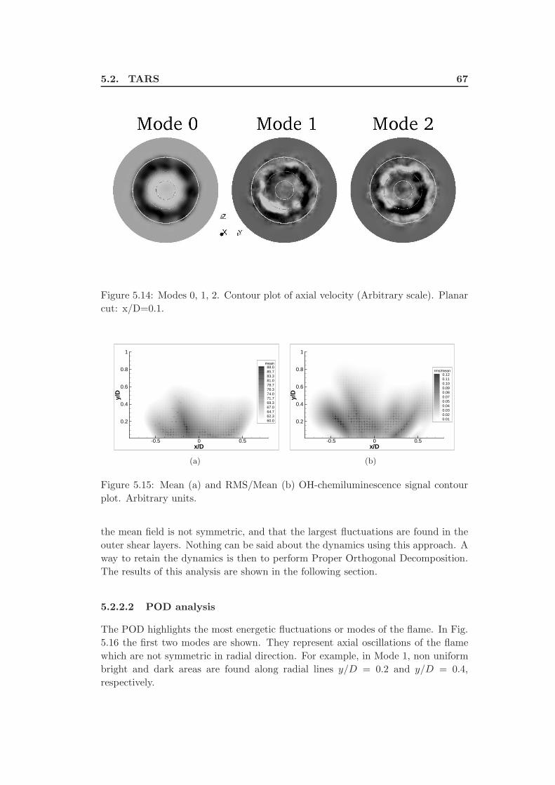
5.2. TARS 67
Figure 5.14: Modes 0, 1, 2. Contour plot of axial velocity (Arbitrary scale). Planar
cut: x/D=0.1.
x/D
y/D
-0.5 0 0.5
0.2
0.4
0.6
0.8
1
mean88.085.783.381.078.776.374.071.769.367.064.762.360.0
(a)
x/D
y/D
-0.5 0 0.5
0.2
0.4
0.6
0.8
1
rms/mean0.120.110.100.090.080.070.050.040.030.020.01
(b)
Figure 5.15: Mean (a) and RMS/Mean (b) OH-chemiluminescence signal contour
plot. Arbitrary units.
the mean field is not symmetric, and that the largest fluctuations are found in the
outer shear layers. Nothing can be said about the dynamics using this approach. A
way to retain the dynamics is then to perform Proper Orthogonal Decomposition.
The results of this analysis are shown in the following section.
5.2.2.2 POD analysis
The POD highlights the most energetic fluctuations or modes of the flame. In Fig.
5.16 the first two modes are shown. They represent axial oscillations of the flame
which are not symmetric in radial direction. For example, in Mode 1, non uniform
bright and dark areas are found along radial lines y/D = 0.2 and y/D = 0.4,
respectively.
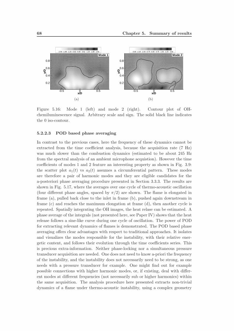
68 Chapter 5. Summary of results
x/D
y/D
-0.5 0 0.5
0.2
0.4
0.6
0.8
: -2.50 -1.88 -1.25 -0.62 0.00 0.62 1.25 1.88 2.50
Mode 1
(a)
x/D
y/D
-0.5 0 0.5
0.2
0.4
0.6
0.8
: -3.00 -2.25 -1.50 -0.75 0.00 0.75 1.50 2.25 3.00
Mode 2
(b)
Figure 5.16: Mode 1 (left) and mode 2 (right). Contour plot of OH-
chemiluminescence signal. Arbitrary scale and sign. The solid black line indicates
the 0 iso-contour.
5.2.2.3 POD based phase averaging
In contrast to the previous cases, here the frequency of these dynamics cannot be
extracted from the time coefficient analysis, because the acquisition rate (7 Hz)
was much slower than the combustion dynamics (estimated to be about 245 Hz
from the spectral analysis of an ambient microphone acquistion). However the time
coefficients of modes 1 and 2 feature an interesting property as shown in Fig. 3.9:
the scatter plot a1(t) vs a2(t) assumes a circumferential pattern. These modes
are therefore a pair of harmonic modes and they are eligible candidates for the
a-posteriori phase averaging procedure presented in Section 3.3.3. The results are
shown in Fig. 5.17, where the averages over one cycle of thermo-acoustic oscillation
(four different phase angles, spaced by π/2) are shown. The flame is elongated in
frame (a), pulled back close to the inlet in frame (b), pushed again downstream in
frame (c) and reaches the maximum elongation at frame (d), then another cycle is
repeated. Spatially integrating the OH images, the heat relase can be estimated. A
phase average of the integrals (not presented here, see Paper IV) shows that the heat
release follows a sine-like curve during one cycle of oscillation. The power of POD
for extracting relevant dynamics of flames is demonstrated. The POD based phase
averaging offers clear advantages with respect to traditional approaches. It isolates
and visualizes the modes responsible for the instability, with their relative ener-
getic content, and follows their evolution through the time coefficients series. This
is precious extra-information. Neither phase-locking nor a simultaneous pressure
transducer acquisition are needed. One does not need to know a-priori the frequency
of the instability, and the instability does not necessarily need to be strong, as one
needs with a pressure transducer for example. One might find out for example
possible connections with higher harmonic modes, or, if existing, deal with differ-
ent modes at different frequencies (not necessarily sub or higher harmonics) within
the same acquisition. The analysis procedure here presented extracts non-trivial
dynamics of a flame under thermo-acoustic instability, using a complex geometry
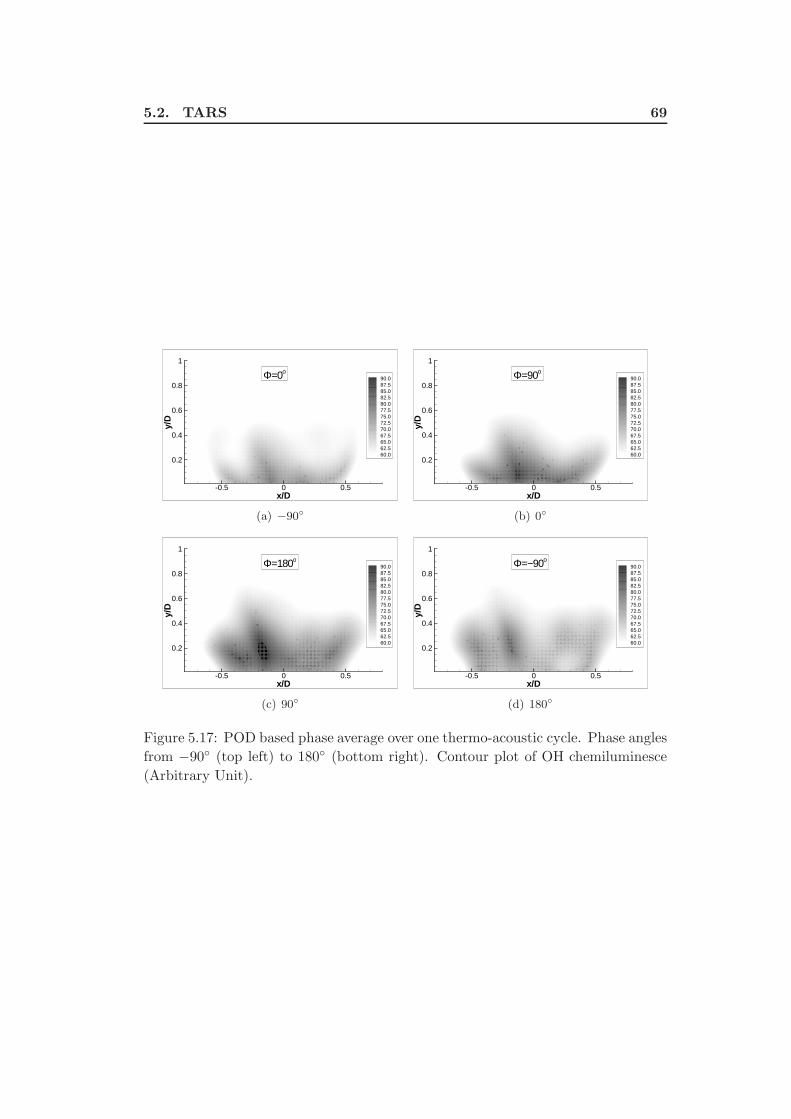
5.2. TARS 69
x/D
y/D
-0.5 0 0.5
0.2
0.4
0.6
0.8
1
90.087.585.082.580.077.575.072.570.067.565.062.560.0
Φ=0ο
(a) −90
x/D
y/D
-0.5 0 0.5
0.2
0.4
0.6
0.8
1
90.087.585.082.580.077.575.072.570.067.565.062.560.0
Φ=90ο
(b) 0
x/D
y/D
-0.5 0 0.5
0.2
0.4
0.6
0.8
1
90.087.585.082.580.077.575.072.570.067.565.062.560.0
Φ=180ο
(c) 90
x/D
y/D
-0.5 0 0.5
0.2
0.4
0.6
0.8
1
90.087.585.082.580.077.575.072.570.067.565.062.560.0
Φ=−90ο
(d) 180
Figure 5.17: POD based phase average over one thermo-acoustic cycle. Phase angles
from −90 (top left) to 180 (bottom right). Contour plot of OH chemiluminesce
(Arbitrary Unit).

70 Chapter 5. Summary of results
burner but relatively simple, cheap, fast to set-up experimental equipment. It there-
fore enables to post-process industrial data where practical and economical issues
often prohibit complex laser diagnostic apparatus.
Chapter 6
Summary of the papers and
author contribution
Paper I
P. Iudiciani and C. Duwig, “Large Eddy Simulation of the sensitivity of vortex
breakdown and flame stabilization to axial forcing”, Flow, Turbulence and Com-
bustion, 86, 639–666, 2011
In this paper, the effect of axial forcing on the flame/vortex breakdown interac-
tion is studied, with particular focus on the PVC. LES, together with a filtered
flamelet model describing the subgrid combustion, is performed to study a lean
premixed flame undergoing mass flow fluctuations in a wide range of frequencies
and amplitude. In average, forcing at frequencies lower than the PVC characteristic
frequency moves the recirculation zone upstream the combustor in the premixing
tube, while higher frequencies do not relevantly affect the flow/flame. With the
help of POD a detailed analysis of the dynamics of the central recirculation zone is
performed showing how the excitation at lower frequencies weakens the PVC and
allows the flame to propagate upstream. Extended POD is also applied to illustrate
the flow/flame interactions during the excitation cycle.
The code, the combustion model and the test case were developed and set-up in
previous works by C. Duwig and L. Fuchs. The candidate carried out the new sim-
ulations, post-processed the results, performed the POD-EPOD analysis and wrote
a major part of the paper under the supervision of C. Duwig.
Paper II
C. Duwig and P. Iudiciani, “Extended Proper Orthogonal Decomposition Anal-
ysis of Flame/Acoustic Interaction”. Flow, Turbulence and Combustion, 84, 25-47,
2010
In this work, simultaneous OH-PLIF and PIV acquisitions of a laminar premixed
flame forced with acoustic waves are used to exemplify and promote the usage of
POD and Extended POD in combustion applications. The concept of Extended
72 Chapter 6. Summary of the papers and author contribution
POD, to highlight the correlations and interaction of flow/flame dynamics, is ap-
plied for the first time in the field of combustion. POD is applied separately on
PIV and PLIF data, both in an unforced and forced case. The PIV-POD performs
well only in the forced case, in which the fluctuations are amplified by the exci-
tations. PLIF-POD instead detects equally well the flame dynamics in both cases
and it is therefore chosen as a suitable base for the EPOD analysis. When applying
the EPOD analysis, the fluctuations in the velocity field are highlighted in both
unforced and forced cases, overcoming problems such as bad seeding in the burnt
gases and low number of available samples.
The data were acquired by the candidate for his Master’s thesis work at the ENEA
Research Centre (New Technologies, Energy and Environment Agency) “Casaccia”
in Rome (Italy) in collaboration with the Department of Mechanics and Aeronautics
of the University of Rome “La Sapienza”. The candidate performed the POD and
EPOD analysis, and wrote the paper together with C. Duwig.
Paper III
P. Iudiciani, C. Duwig, R.Z. Szasz, L. Fuchs, S.M. Hosseini, and E.J.
Gutmark, “LES investigation of the flow dynamics in a realistic gas turbine multi-
swirl fuel-injector”. Manuscript, submitted to AIAA journal, 2012
In this paper, the flow through a fuel-injector with three swirlers, the TARS, has
been studied by means of Large Eddy Simulation and PIV measurements. Good
agreement was found between the computational and experimental data highlight-
ing also the features of the flow inside the TARS burner. Sensitivity to the grid
and to the SGS model was determined to be within the range of experimental un-
certainty. The flow azimuthal structure was shown to be mainly affected by the
flow passage through multiple vanes of the three swirlers, and by the upstream
structure that supports the fuel injector and supply fuel. Precise inlet boundary
conditions that include these geometrical elements were critical to obtain accu-
rate prediction of the complex flow structure. This finding is important because
practical combustor in aeroengines have similar geometry which is often ignored
in experimental and computational investigations. Proper Orthogonal Decompo-
sition analysis helped to separate coherent structures from the complex turbulent
flow, revealing the existence of helical structures leading to a precessing vortex core.
The candidate carried out the LES simulations, post-processed the results, and wrote
a major part of the paper, with additions from S.M. Hosseini, under the supervision
of E. Gutmark, C. Duwig, R.Z. Szasz and L. Fuchs.
73
Paper IV
P. Iudiciani, C. Duwig, S.M. Hosseini, R.Z. Szasz, L. Fuchs and E.J.
Gutmark, “Proper Orthogonal Decomposition for experimental investigation of
swirling flame instabilities”. Accepted for publication in AIAA journal, to appear
2012
An experimental investigation of premixed flames undergoing thermo-acoustic in-
stability is presented. The paper focuses on the data post-processing, aiming at
extracting information about the dynamics that are lost through classical time
averaging approach. Proper Orthogonal Decomposition together with a derived a-
posteriori phase averaging procedure are applied to OH* chemiluminescence data,
obtained with a simple experimental set-up at low acquisition rate. The combus-
tion dynamics are successfully reconstructed from the raw data, without the need
of extra acquisitions or of phase locking the measurements, and providing extra-
information about the instability modes. The method was validated against high
speed camera direct light measurements. In an intermittent case close to bifurca-
tion, the procedure further helps to sort out different states of the flame.
The candidate participated to the experimental campaign. The experimental rig was
set-up by M.S. Hosseini, and R.Z. Szasz. The candidate post-processed the results
and performed the POD analysis. The candidate wrote a major part of the paper,
with additions from S.M. Hosseini, and the supervision of E. Gutmark, C. Duwig,
R.Z. Szasz and L. Fuchs.
Paper V
P. Iudiciani, C. Duwig, R.Z. Szasz, L. Fuchs, S.M. Hosseini and E.J.
Gutmark, “Numerical and experimental investigation of swirling flows and flames
generated through a multi-swirl fuel injector”. ISABE-2011-1132, 12-16 September
2011, Gothenburg, Sweden
In this paper, reacting flows in a complex geometry fuel injector of interest for
aero-engines applications have been simulated by means of LES. The proposed
formulation captures well the dynamics of the flow/flame in a stable case. For dif-
ferent operating conditions, a dual behaviour is observed, in which stabilization in
the wake of the burner and flashback coexists depending on the initial conditions.
Useful insights about the flame holding mechanism are provided. The LES results
are in qualitative agreement with the experimental measurements.
The candidate carried out the LES simulations, post-processed the results, and wrote
a major part of the paper, with additions from S.M. Hosseini, under the supervision
of E. Gutmark, C. Duwig, R.Z. Szasz and L. Fuchs.
74 Chapter 6. Summary of the papers and author contribution
Paper VI
P. Iudiciani, C. Duwig, R.Z. Szasz, L. Fuchs and E.J. Gutmark, “LES
of the interaction between a premixed flame and complex turbulent swirling flow”.
13th European Turbulence Conference ETC13. Journal of Physics: Conference Se-
ries, 318(9):092007
In this paper the TARS, a fuel injector characterized by complex design with three
concentric air passages, has been studied numerically. A swirl-stabilized lean pre-
mixed flame has been simulated by means of LES. The computations characterize
successfully the dynamics of the flame and their interactions with the complex
swirling flow. The flame is stabilized upstream the fuel injector exit, and the dy-
namics are led by a PVC which seems to originate in the inner air passage. The
results obtained by POD analysis are in agreement with previous findings in the
context of swirling flows/flames.
The candidate carried out the LES simulations, post-processed the results, and wrote
a major part of the paper, under the supervision of E. Gutmark, C. Duwig, R.Z.
Szasz and L. Fuchs.
Chapter 7
Conclusions and future work
7.1 Conclusions
In this work, advanced techniques (LES, POD, and optical diagnostic techniques)
have been applied to analyze swirl stabilized flames, relevant to gas turbine appli-
cations. The methods used enhance the understanding swirling flame dynamics. In
particular, Large Eddy Simulations of a forced flame (the so called Lisbon burner)
showed the influence of axial oscillations on the flame stabilization by vortex break-
down. Forcing at frequencies lower than the PVC weakened the PVC itself allow-
ing the flame to stabilize more upstream, while frequencies equal or higher than
the PVC did not significantly affect the flame stabilization. Lock-in of the PVC
with the excitation frequency was not observed. Moreover the mean flame front
was found not to coincide with the shear-layer surrounding the CRZ because of the
PVC motion.
For the TARS burner, the LES presented here clarified the details of the complex
flow through the fuel-injector, and characterized the dynamics of the swirling flow
downstream the TARS. In order to reduce uncertainties, the LES simulation of
the complete burner was carried out, including relevant details of the rig, such as
the support arm and fuel supply pipes upstream the TARS. It was shown that the
upstream details play an important role for the variability of the azimuthal structure
in an isothermal case. An LES formulation with finite rate chemistry was tested
in reacting cases. The formulation was able to explain the peculiar stabilization
mechanism in a case where the CRZ was destroyed by thermal expansion, to capture
dual behavior/hysteresis phenomena, to describe the dynamics of a lean flame and
its interaction with the PVC. The present formulation is therefore promising for
the more detailed study of selected test-cases from the current and future database
of experiments.
The analyses presented in this thesis included Proper Orthogonal Decomposi-
tion applied to both numerical and experimental data in order to explore the flame
dynamics. Large scale flow and flame fluctuations due to coherent structures have
been highlighted in different academic combustors encouraging the use of Proper
Orthogonal Decomposition in combustion applications. A POD-based a-posteriori
phase averaging procedure was used to study combustion dynamics, enabling the re-
construction of cycles of thermo-acoustic instabilities. Using a simple and relatively
cheap set-up, such technique may be applied for in-situ industrial measurements.
Finally, this work introduced the usage of Extended POD for the analysis of
the interaction between flow and flame dynamics. Such technique was applied
76 Chapter 7. Conclusions and future work
for the first time in the context of reacting flows. In particular it highlighted the
mechanism by which axial oscillations weaken the PVC in a swirl-stabilized flame in
the numerical study mentioned above. Applied in an experimental study, it related
the dynamics of a laminar flame to vortex shedding in the shear layers.
7.2 Future work
Recently, the TARS test-rig has been modified to include a premixing tube added
at the TARS outlet and both confined and unconfined flames have been measured.
The goal is to study the influence of vortex breakdown on flame stabilization and
flashback. In particular the mutual positions of the recirculation zone and the
flame position are addressed. Effects of varying equivalence ratios are considered.
Simulations of these new test-cases would certainly positively complement the ex-
perimental results. Some limiting assumptions should still be listed as base for
further work. First, the assumption of adiabatic walls might be refined, especially
inside the swirler vanes since they are thin and rather close to the flame. In order
to capture the possible complex stabilization at the swirler edges, more refined wall
temperature modeling as well as a detailed chemical mechanism might be required.
Clearly, these new databases will also open new possibilities to confirm the
validity of POD and EPOD analysis to address the dynamics of swirling flows and
flames.
Acknowledgements
This thesis is the result of the four years that I spent at the division of Fluid
Mechanics, Lund University. At the end of this journey a few people should be
thanked, to have made this possible, valuable, and fun.
Firstly, I would like to acknowledge my supervisor, Prof. Laszlo Fuchs, for giving
me the opportunity to join the group. Thank you for always being stimulative
towards scientific critical thinking and for continuously reminding what it means to
do re-search.
A grateful thank goes to my co-supervisor, Dr. Christophe Duwig, for being
the motor of this research (re-search, sorry Laszlo!) project. Thank you for all
the precious discussions about combustion, dynamics of swirling flows and flames,
POD, and for the friendliness demonstrated during these years. Especially, thank
you for the extreme rapidity, simplicity and efficiency in answering my e-mails! Now
you can tell me your secret, how do you manage?!
Many thanks go to my other co-supervisor, Dr. Robert Szasz, for always kindly,
friendly and readily answering all my questions about CFD. Thank you for helping
me with computer related issues and for introducing me to the wonderful world of
Linux. Can I finally get the root password now?!
I would also like to acknowledge Prof. Effie Gutmark for all the valuable discus-
sions and suggestions. Thank you for always making me feel at ease while sharing
your vast experience during your visits to Lund.
Robert Collin, Andreas Lantz, and Mohammad Seyed Hosseini are also acknowl-
edged for the great work done during the experiments in the lab.
The simulations were run on several computational centers throughout Sweden:
LUNARC at Lund University, Akka at Umea University, PDC at the Royal Institute
of Technology in Stockholm.
This work would not have been possible without the entities who financially
supported the project: Vetenskap Radet (VR), the Centre for Combustion Science
and Technology (CECOST) and the Swedish energy authority (STEM).
Therefore, thanks to the Swedish tax payers, who indirectly finance these insti-
tutions. About this, I would like to remark that, being an Italian, the first time
I read such an acknowledgement in previous theses, I thought it was written with
irony! How many things you have taught me during these years, dear Sverige.
I also want to thank and salute all my colleagues, present and past ones, at the
divisions of fluid mechanics and combustion physics. More in particular, thank you:
Eric “typically”Baudoin, for leaving the entire office for me. Just kidding. Se-
riously, thanks because since you left we do not go to Finn Inn anymore. Kidding
again, you were a great office mate and friend!
“Giovane Esploratore”Tobias Joelsson, aka “Wolf”, for allowing me to contem-
porarily obtain a Ph.D. on the Vietnam War. Thank you also for constant good
mood and smiles!
78 Chapter 7. Conclusions and future work
Holger “Oliver”Grosshans, for having spent uncountable hours together trying
to find the analytical solution of the NS equations. I hope you will mention me
while holding the speech for your future Nobel Prize. Which, I remind you though,
we have higher chances to win for peace in the world. Let’s love turbulence and use
it for change!
Jiangfei and Fan, for always bringing me back nice gifts from China;
Rixin and Mehdi, for never banal discussions at Fysikum about work related
topics, and non;
Alper, Hesam, Aurelia, Rickard and Henning, thank you for being a very nice
regular company during lunches and (a bit less regular, unfortunately) evening
beers.
Then, it’s your turn, my dear Lundian friend. If you ever got to read this thesis,
well first thank you because it means that you probably came to listen to the boring
dissertation! I will name only you who actually have some chances to actually read
this! So, in kind of chronological order, thank you Ale “De Andre”Barni, Julioccini,
Adri Le“t’s dance”pur, the “apples”Keyvan and Viveka, Moe “that’s a good ques-
tion”Takemura, Anna “once in a lifetime”Beek, Michele “che boss”Giunta, Anna
“baking queen”G (som Gemma!), Cristin “what is this?”Giessler, and all of you
guys it would take for ever to mention. I heartily thank you for all the lovely time
spent together in Lund during the last four years.
Biggest thanks and love to Emilijute, for making the last two years even more
special. My wish is that one day we will write a paper together about the turbulence
of indian slums!
Infine, un sentito grazie ai miei genitori, Francesca and Tonio, e alla mia sorellina
cairota Laura. Mi dispiace tanto di non trascorrere abbastanza tempo insieme a
voi, tuttavia e un sollievo sapere che il baricentro della famiglia resta sempre in
Abruzzo!
Bibliography
[1] International Energy Agency. Key world energy statistics. Technical report,
IEA report, 2009.
[2] Princeton Environmental Institute. Princeton’s next generation
jet fuel project. Technical report, Princeton University, 2009.
http://www.princeton.edu/pei/energy/presentations/, last access april
2010.
[3] A.H. Lefebvre. The role of fuel preparation in low-emission combustion. Jour-
nal of Engineering for Gas Turbines and Power, 117, 1995.
[4] D.W. Bahr. Gas turbine combustion and emission abatment technology.
current and projected status. Proceedings of the International Gas Turbine
Congress 1999 Kobe, 1999.
[5] Y. Huang and V. Yang. Dynamics and stability of lean-premixed swirl-
stabilized combustion. Progress in Energy and Combustion Science,
35(4):293–364, 2009. doi:10.1016/j.pecs.2009.01.002.
[6] T. Lieuwen. Combustion dynamics in lean-premixed prevaporized (LPP) gas
turbines. Journal of Propulsion and Power, 19, 2003.
[7] O. Lucca-Negro and T. O’Doherty. Vortex breakdown: a review. Progress
in Energy and Combustion Science, 27(4):431–481, 2001. doi:10.1016/S0360-
1285(00)00022-8.
[8] Y. Sommerer, D. Galley, T. Poinsot, S. Ducruix, F Lacas, and D. Veynante.
Large eddy simulation and experimental study of flashback and blow-off in a
lean partially premixed swirled burner. Journal of Turbulence, 5, 2004.
[9] M. Konle, F. Kiesewetter, and T. Sattelmayer. Simultaneous high repetition
rate PIV-LIF measurements of CIVB driven flashback. Exp. Fluids, 44:529–
538, 2008.
[10] S. Nair and T. Lieuwen. Near-blowoff dynamics of a bluff-body stabilized
flame. Journal of Propulsion and Power, 23(2):421–427, 2007.
[11] E. Gutmark, T.P. Parr, D.M. Parr, and K.C. Schadow. Evolution of vortical
structures in flames. Twenty-Second International Symposium on Combus-
tion/The Combustion Institute, pages 523–529, 1988.
[12] Balachandran et al. Experimental investigation of the nonlinear response
of turbulent premixed flames to imposed inlet velocity oscillations. Comb.
Flame, 143:37–55, 2005.
80 Bibliography
[13] O.J. Teerling, A.C. McIntosh, J. Brindley, and V.H.Y Tam. Premixed flame
response to oscillatory pressure waves. Proceedings of the Combustion Insti-
tute, 30:1733–1740, 2005.
[14] S. Shanbhogue and T. Lieuwen. Studies on the vorticity field of harmonically
excited bluff body flames. 46th AIAA Aerospace Sciences Meeting and Exhibit,
AIAA 2008–122. Reno, USA, 2008.
[15] T. Schuller, D. Durox, and S. Candel. Self-induced combustion oscillations
of laminar pre-mixed flames stabilized on annular burners. Comb. Flame,
135:525–537, 2003.
[16] D. Durox, S. Ducruix, and S. Candel. Experiments on collapsing cylindrical
flames. Comb. Flame, 125:982–1000, 2001.
[17] S. Candel, D. Durox, S. Ducruix, A. L. Birbaud, N. Noiray, and T. Schuller.
Flame dynamics and combustion noise: progress and challenges. International
Journal of Aeroacoustics, 8(1-2):1–56, 2009.
[18] R. Szasz, C. Duwig, and L. Fuchs. Noise generated by a lifred flame in a
vitiated co-flow. Proceedings of ASME Turbo Expo 2008: Power for Land,
Sea and Air, GT2008-51186, 2008.
[19] C. Duwig, L. Fuchs, A. Lacarelle, M. Beutke, and C.O. Paschereit. Study
of the vortex breakdown in a conical swirler using LDV, LES and POD.
Proceedings of ASME Turbo Expo 2007, GT2007-27006, 2007.
[20] S.I. Shtork, N.F. Vieira, and E.C. Fernandes. On the identification of heli-
cal instabilities in a reacting swirling flow. Fuel, 87(10-11):2314–2321, 2008.
doi:10.1016/j.fuel.2007.10.016.
[21] N. Syred. A review of oscillation mechanisms and the role of the precessing
vortex core (PVC) in swirl combustion systems. Progress in Energy and
Combustion Science, 32(2):93–161, 2006. doi:10.1016/j.pecs.2005.10.002.
[22] F. Martinelli, A. Olivani, and A. Coghe. Experimental analysis of the pre-
cessing vortex core in a free swirling jet. Exp. Fluids, 42(6):827–839, 2007.
doi:10.1007/s00348-006-0230-x.
[23] P.M. Anacleto, E.C. Fernandes, M.V. Heitor, and S.I Shtork. Swirl flow struc-
ture and flame characteristic in a model lean premixed combustor. Combust.
Sci. and tech., 175:1369–1388, 2003.
[24] C. Duwig and L. Fuchs. Large eddy simulation of vortex breakdown/flame
interaction. Phys. Fluids, 19(075103), 2007. doi:10.1063/1.2749812.
[25] M. Stohr, R. Sadanandan, and W. Meier. Experimental study of unsteady
flame structures of an oscillating swirl flame in a gas turbine model combustor.
Proceedings of the Combustion Institute, 32:2952–2932, 2009.
Bibliography 81
[26] S. Khalil, K. Hourigan, and M.C. Thompson. Response of unconfined vortex
breakdown to axial pulsing. Phys. Fluids, 18, 2006.
[27] S.V. Alekseenko et al. Effect of axisymmetric forcing on the structure of a
swirling turbulent jet. International Journal of Heat and Fluid Flow, 29:1699–
1715, 2008.
[28] S. Wang, S.Y. Hsieh, and V.Yang. Unsteady flow evolution in swirl injector
with radial entry. II. External excitation. Phys. Fluids, 17(045107), 2005.
doi:10.1063/1.1874932.
[29] F. Gallaire, S. Rott, and J.M. Chomaz. Experimental study of a free and
force swirling jet. Phys. Fluids, 16, 2004.
[30] A. Lacarelle, T. Faistmann, D. Greenblatt, C.O. Paschereit, O. Lehmann,
D.M. Luchtenburg, and B.R. Noach. Spatio-temporal characterization of a
conical swirler flow field under strong forcing. Journal of Engineering for Gas
Turbine and Power, 131(031504), 2009. doi:10.1115/1.2982139.
[31] K. Oberleithner, M. Sieber, C.N. Nayeri, C.O. Paschereit, C. Petz, H.-C. Hege,
B.R. Noack, and I. Wygnasnki. Three-dimensional coherent structures in a
swirling jet undergoing vortex breakdown: stability analysis and empirical
mode construction les of chemical and acoustic forcing of a premixed dump
combustor. J. Fluid. Mech., 679:383–414, 2011. doi:10.1017/jfm.2011.141.
[32] C.O. Paschereit, E. J. Gutmark, and W. Weisenstein. Coherent structures
in swirling flows and their role in acoustic combustion control. Phys. Fluids,
11(9):2667–2678, 1999.
[33] D.M. Kang, F.E.C. Culick, and A. Ratner. Combustion dynamics of a low-
swirl combustor. Comb. Flame, 151:412–425, 2007.
[34] S.K. Thumuluru and T. Lieuwen. Characterization of acoustically forced
swirl flame dynamics. Proceedings of the Combunstion Institute, 32:2893–
2900, 2009.
[35] B.D. Bellows, M.K. Bobba, A. Forte, J.T. Seitzman, and T. Lieuwen. Flame
transfer function saturation mechanism in a swirl-stabilized combustor. Pro-
ceedings of the Combustion Institute, 31:3181–3188, 2007.
[36] P. Palies, D. Durox, T. Schuller, and S. Candel. The combined dynamics
of swirler and turbulent premixed swirling flames. Combustion and Flame,
157(9):1698–1717, 2010.
[37] Uyi Idahosa, Abhishek Saha, Chengying Xu, and Saptarshi Basu. Non-
premixed acoustically perturbed swirling flame dynamics. Combustion and
Flame, 157(9):1800–1814, 2010.
82 Bibliography
[38] K.T. Kim, J.G. Lee, B.D. Quay, and D.A. Santavicca. Spatially distributed
flame transfer functions for predicting combustion dynamics in lean premixed
gas turbine combustors. Combustion and Flame, 157(9):1718–1730, 2010.
[39] A.M. Steinberg, I. Boxx, M. Stohr, C.D. Carter, and W. Meier. Flow-flame
interactions causing acoustically coupled heat release fluctuations in a thermo-
acoustically unstable gas turbine model combustor. Combustion and Flame,
157(12):2250–2266, 2010.
[40] U. Piomelli. Large-eddy simulation: achievements and challenges. Progress in
Aerospace Sciences, 35(4):335–362, 1999. doi:10.1016/S0376-0421(98)00014-1.
[41] C.M. Coats. Coherent structures in combustion. Prog in Energy and Comb.
Sci., 22:427–509, 1996.
[42] C.E. Cala, E.C. Fernandes, M.V. Heitor, and S.I. Shtork. Coherent structures
in unsteady swirling jet flow. Exp. Fluids, 40:267–276, 2006.
[43] G. Berkooz, P. Holmes, and J.L. Lumley. The proper orthogonal decomposi-
tion in the analysis of turbulent flows. Annu. Rev. Fluid Mech., 25:539–575,
1993. doi:10.1146/annurev.fl.25.010193.002543.
[44] T. Smith, J. Moehlis, and P. Holmes. Low-dimensional modelling of turbu-
lence using the proper orthogonal decomposition. a tutorial. Nonlinear Dyn.,
41:275–307, 2005.
[45] L. Perret, J. Delville, R. Manceau, and J.P. Bonnet. Turbulent inflow con-
ditions for large-eddy simulation based on low-order empirical model. Phys.
Fluids, 20, 2008.
[46] S. Bernero and H.E. Fiedler. Application of particle image velocimetry and
proper orthogonal decomposition to the study of a jet in a counterflow. Exp.
Fluids, 29:274–281, 2000.
[47] K.E. Meyer, J.M. Pedersen, and O. Ozcan. A turbulent jet in crossflow anal-
ysed with proper orthogonal decomposition. J. Fluid Mech., 583:199–227,
2007.
[48] K. Bizon, G. Continillo, E. Mancaruso, S.S. Merola, and B.M. Veglieco. POD-
based analysis of combustion images in optically accessible engines. Comb.
Flame, 157(4):632–640, 2010.
[49] C. Alvarez-Herrera, D. Moreno-Hernandez, and B. Barrientos-Garcia. Tem-
perature measurement of an axisymmetric flame by using a schlieren system.
J. Optics A-Pure and Applied Optics, 2008.
[50] H.G. Sung. Combustion dynamics in a model lean-premixed gas turbine with
a swirl stabilized injector. J. Mech. Sci. and Technology, 21(3):495–504, 2007.
Bibliography 83
[51] X.M. Huang and W.T. Baumann. Reduced-order modeling of dynamic heat
release for thermoacoustic instability prediction. Comb Sci Tech., 179(3):617–
636, 2007.
[52] A. Kodal et al. Turbulence filter and POD analysis for velocity fields in lifted
CH4-air diffusion flames. Flow, Turbulence and Combustion, 70:21–41, 2003.
[53] A. Lacarelle, D.M. Luchtenburg, M.R. Bothien, B.R. Noack, and C.O.
Paschereit. A combination of image post-processing tools to identify coher-
ent structures of premixed flames. Int. Conf. on Jets, Wakes and Separated
Flows, ICJWSF-2008, 16-19 September 2009, Berlin, Germany, 2009.
[54] C. Duwig and L. Fuchs. Large eddy simulation of a H2/N2 lifted flame in a
vitiated coflow. Comb. Sci. and Tech., 180(3):453–480, 2008.
[55] A. Roux, L.Y.M. Gicquel, Y. Sommerer, and T.J. Poinsot. Large eddy sim-
ulation of mean and oscillating flow in a side-dump ramjet combustor. Com-
bustion and Flame, 152(1-2):154–176, 2008.
[56] B. W. van Oudheusden, F. Scarano, N. P. van Hinsberg, and D. W. Watt.
Phase-resolved characterization of vortex shedding in the near wake of a
square-section cylinder at incidence. Experiments in Fluids, 39:86–98, 2005.
[57] Tony Ruiz, C. Sicot, L. Brizzi, J. Boree, and Y. Gervais. Pressure/velocity
coupling induced by a near wall wake. Experiments in Fluids, 49:147–165,
2010.
[58] S. Maurel, J. Boree, and J.L. Lumley. Extended proper orthogonal decompo-
sition: Application to jet/vortex interaction. Flow, Turbulence and Combus-
tion, 67:125–136, 2001.
[59] J. Boree. Extended proper orthogonal decomposition: a tool to analyse cor-
related events in turbulent flows. Experiments in Fluids, 35:188–192, 2003.
[60] E.C. Fernandes, M.V. Heitor, and S.I. Shtork. An analysis of unsteady highly
turbulent swirling flow in a model vortex combustor. Exp. Fluids, 40(2):177–
187, 2006. doi:10.1007/s00348-005-0034-4.
[61] P. Iudiciani and C. Duwig. Large eddy simulation of the sensitivity of vortex
breakdown and flame stabilisation to axial forcing. Flow, Turbulence and
Combustion, 86:639–666, 2011.
[62] C. Duwig and P. Iudiciani. Extended proper orthogonal decomposition analy-
sis of flame/acoustic interaction. Flow, Turbulence and Combustion, 84(1):25–
47, 2010. doi:10.1007/s10494-009-9210-6.
[63] G. Li and E.J. Gutmark. Effect of exhaust nozzle geometry on combustor flow
field and combustion characteristics. Proceedings of the Combustion Institute,
30(2):2893–2901, 2005. doi:10.1016/j.proci.2004.08.189.
84 Bibliography
[64] P. Iudiciani, C. Duwig, R.Z. Szasz, L. Fuchs, S.M. Hosseini, and E.J. Gutmark.
LES investigation of the flow dynamics in a realistic gas turbine multi-swirl
fuel-injector. Manuscript, submitted to AIAA journal, 2012.
[65] P. Iudiciani, C. Duwig, S.M. Hosseini, R.Z. Szasz, L. Fuchs, and E.J. Gut-
mark. Proper orthogonal decomposition for experimental investigation of
flame instabilities. Accepted for publication in AIAA journal, to appear, 2012.
[66] P. Iudiciani, C. Duwig, R.Z. Szasz, L. Fuchs, S.M. Hosseini, and E.J. Gut-
mark. Numerical and experimental investigation of swirling flows and flames
generated through a multi-swirl fuel injector. In ISABE-2011-1132, 12-16
September 2011, Gothenburg, Sweden.
[67] P. Iudiciani, C. Duwig, R.Z. Szasz, L. Fuchs, and E.J. Gutmark. LES
of the interaction between a premixed flame and complex turbulent
swirling flow. Journal of Physics: Conference Series, 318(9):092007, 2011.
doi:10.1088/1742-6596/318/9/092007.
[68] O. Reynolds. An experimental investigation of the circumstances which de-
termine wheter the motion of water shall be direct or sinuous, and the law
of resistance in parallel channels. Philos. Trans. R. Soc. London Ser. A174,
pages 935–982, 1883.
[69] S. Pope. Turbulent Flows. Cambridge University Press, 2000.
[70] T. Poinsot and D. Veynante. Theoretical and Numerical Combustion. Ed-
wards, 2000.
[71] G. Smith, T. Bowman, M. Frenklach, B. Gardiner, et al. GRI mechanism.
http://www.me.berkeley.edu/gri-mech/, last access june 2011.
[72] S. Turns. An introduction to combustion. McGraw-Hill, 2000.
[73] A.H. Lefebvre. Gas Turbine Combustion, second edition. Taylor and Francis,
1999.
[74] C. Duwig, D. Stankovic, L. Fuchs, G. Li, and E.J. Gutmark. Experimental and
numerical study of flameless combustion in a model gas turbine combustor.
Combust. Sci. and Tech., 180:279–295, 2000.
[75] P.J. Coelho and N. Peters. Numerical simulation of a mild combustion burner.
Comb. Flame, 124:503–518, 2001.
[76] Antonio Cavaliere and Mara de Joannon. Mild combustion. Progress in
Energy and Combustion Science, 30(4):329–366, 2004.
[77] E. Mallard and H.L. Le Chatelier. Recherches experimentales et theoriques
sur la combustion des melanges gazeux explosifs. Ann. des Mines, 1883.
Bibliography 85
[78] C. Fureby. On subgrid scale modeling in large eddy simulations of compress-
ible fluid flow. Physics of Fluids, 8(5):1301–1311, 1996.
[79] J. Smagorinsky. General circulation experiments with the primitive equations:
I. the basic equations. Mon. Weather Review, 91:99–164, 1963.
[80] J. Bardina, J.H. Ferziger, and W.C. Reynolds. Improved subgrid-scale models
for large-eddy simulation. AIAA Paper No., (80-1357), 1980.
[81] A. Germano, U. Piomelli, P. Moin, and W.H. Cabot. A dynamic subgrid-scale
eddy viscosity model. Phys. Fluids, 3:1760–1765, 1991.
[82] D.K. Lilly. A proposed modification of the Germano subgrid-scale closure
method. Phys. Fluids A, 4:633, 1991. doi:10.1063/1.858280.
[83] P. Sagaut, P. Comte, and F. Ducros. Filtered subgrid-scale models. Physics
of Fluids, 12(1):233–236, 2000.
[84] L. G. Margolin, W. J. Rider, and F. F. Grinstein. Modeling tur-
bulent flow with implicit LES. Journal of Turbulence, 7(15), 2006.
doi:10.1080/14685240500331595.
[85] C. Fureby and F.F. Grinstein. Monotonically integrated large eddy simulation
of free shear flows. AIAA journal, 37(5), 1999.
[86] C. Fureby. ILES and LES of complex engineering turbulent flows. Journal of
Fluids Engineering, 129:1514–1523, 2007.
[87] F.F. Grinstein, T.R. Young, E.J. Gutmark, G. Li, G. Hsiao, and H.C. Mongia.
Flow dynamics in a swirl combustor. Journal of Turbulence, 3(030), 2002.
doi:10.1088/1468-5248/3/1/030.
[88] C. Duwig and L. Fuchs. Study of flame stabilization in a swirling combustor
using a new flamelet formulation. Combust. Sci. and tech., 177:1485–1510,
2005.
[89] C. Duwig and C. Fureby. Large eddy simulation of unsteady lean stratified
premixed combustion. Comb. and Flame, 151:85–103, 2007.
[90] C. Duwig. Study of a filtered flamelet formulation for large eddy simulation
of premixed turbulent flames. Flow, Turbulence and Combustion, 2007.
[91] H. Pitsch. Large-eddy simulation of turbulent combus-
tion. Annual Review of Fluid Mechanics, 38(1):453–482, 2006.
doi:10.1146/annurev.fluid.38.050304.092133.
[92] J. Janicka and A. Sadiki. Large eddy simulation of turbulent combustion
systems. Proceedings of the Combustion Institute, 30(1):537 – 547, 2005.
doi:10.1016/j.proci.2004.08.279.
86 Bibliography
[93] C. Duwig, K-J. Nogenmyr, C-K. Chan, and M.J. Dunn. Large eddy simula-
tions of a piloted lean premix jet flame using finite-rate chemistry. Combustion
Theory and Modelling, 15(4):537–568, 2011.
[94] L. Selle, G. Lartigue, T. Poinsot, R. Koch, K. U. Schildmacher, W. Krebs,
B. Prade, P. Kaufmann, and D. Veynante. Compressible large-eddy simula-
tion of turbulent combustion in complex geometry on unstructured meshes.
Combustion and Flame, 137(4):489–505, 2004.
[95] O. Kruger, K. Gockeler, S. Goke, C. O. Paschereit, C. Duwig, and L. Fuchs.
Numerical investigations of a swirl-stabilized premixed flame at ultra-wet con-
ditions. GT2011-45866, Proceedings of ASME Turbo Expo 2011, Vancouver,
Canada, 2011.
[96] O. Colin, F. Ducros, D. Veynante, and T. Poinsot. A thickened flame model for
large eddy simulations of turbulent premixed combustion. Physics of Fluids,
12(7):1843–1863, 2000.
[97] T.D. Butler and P.J. O’Rourke. A numerical method for two-dimensional
unsteady reacting flows. 16th Int. Symp. on Combustion. the Combustion
Institute, 1977.
[98] V. Raman and H. Pitsch. A consistent les/filtered-density function
formulation for the simulation of turbulent flames with detailed chem-
istry. Proceedings of the Combustion Institute, 31(2):1711 – 1719, 2007.
doi:10.1016/j.proci.2006.07.152.
[99] A.R. Kerstein, W. Ashurt, and K. W. Williams. Field equation for interface
propagation in an unsteady homogeneous field. Phys. Rev., 37, 1988.
[100] N. Peters. The turbulent burning velocity for large-scale and small-scale tur-
bulence. Journal of Fluid Mechanics, 384(1):107–132, 1999.
[101] H. Pitsch and L. Duchamp de Lageneste. Large-eddy simulation of premixed
turbulent combustion using a level-set approach. Proceedings of the Combus-
tion Institute, 29(2):2001 – 2008, 2002. doi:10.1016/S1540-7489(02)80244-9.
[102] K.-J. Nogenmyr, C. Fureby, X.S. Bai, P. Petersson, R. Collin, and M. Linne.
Large eddy simulation and laser diagnostic studies on a low swirl stratified
premixed flame. Combustion and Flame, 156(1):25–36, 2009.
[103] M. Boger, D. Veynante, H. Boughanem, and A. Trouve. Direct numerical
simulation analysis of flame surface density concept for large eddy simulation
of turbulent premixed combustion. 27th Int. Symp. on Combustion, 1998.
[104] C. Fureby. A fractal flame-wrinkling large eddy simulation model for premixed
turbulent combustion. Proceedings of the Combustion Institute, 30, 2005.
Bibliography 87
[105] C. Meneveau and T. Poinsot. Stretching and quenching of flamelets in pre-
mixed turbulent combustion. Comb. Flame, 86, 1991.
[106] H.G. Weller, G. Tabor, A.D. Gosman, and C. Fureby. Application of a flame-
wrinkling LES combustion model to a turbulent mixing layer. Twenty-Seventh
Symposium (International) on Combustion/The Combustion Institute, 1998.
[107] Sebastien Candel. Combustion dynamics and control: Progress and chal-
lenges. Proceedings of the Combustion Institute, 29(1):1–28, 2002.
[108] H.C. Mongia, T.J. Held, G.C. Hsiao, and R.P. Pandalai. Challenges and
progress in controlling dynamics in gas turbine combustors. Journal of Propul-
sion and Power, 19(5):822–829, 2003.
[109] J.H. Ferziger and M. Peric. Computational Methods for Fluid Dynamics.
Springer, 1999.
[110] 1.J. Gullbrand, X.S. Bai, and L. Fuchs. High-order cartesian grid method for
calculation of incompressible turbulent flows. Int. J. Numer. Methods Fluids,
36, 2001.
[111] http://www.openfoam.com, last access April 2011.
[112] H.G. Weller, G. Tabor, H. Jasak, and C. Fureby. A tensorial approach to com-
putational continuum mechanics using object-oriented techniques. Computers
in physics, 12(6):620–631, 1998. doi:10.1063/1.168744.
[113] R. Mittal and G. Iaccarino. Immersed boundary methods. Annu. Rev. Fluid
Mech., 37:239–261, 2005.
[114] G.S. Jang and C.W. Shu. Efficient implementation of weighted ENO schemes.
J. Comput. Phys., 126:202–228, 1996.
[115] A. Harten, B. Engquist, S. Osher, and S. Chakravarthy. Uniformly high
order accurate essentially non-oscillatory schemes, III. J. Comput. Phys.,
71(2):231–303, 1987. doi:10.1016/0021-9991(87)90031-3.
[116] H. Jasak. Error analysis and estimation for the Finite Volume method with
applications to fluid flows. Doctoral thesis, Imperial College, 1996.
[117] J. Kiefer, Z.S. Li, J. Zetterberg, X.S. Bai, and M. Alden. Investigation of
local flame structures and statistics in partially premixed turbulent jet flames
using simultaneous single-shot CH and OH planar laser-induced fluorescence
imaging. Comb. Flame, pages 802–818, 2008.
[118] S.A. Filatyev, M.P. Thariyan, R.P. Lucht, and J.P. Gore. Simultaneous stereo
particle image velocimetry and double-pulsed planar laser-induced fluores-
cence of turbulent premixed flames. Comb. Flame, 150(3):201–209, 2007.
88 Bibliography
[119] A. C. Eckbreth. Laser diagnostics for combustion temperature and species.
Gordon and Breach Publishers, 1996.
[120] L. Sirovich. Turbulence and the dynamics of coherent structures. part 1:
coherent structures. Quart. App. Math., XLV, 3:561–571, 1987.
[121] N. Aubry. On the hidden beauty of proper orthogonal decomposition. Theoret.
Comput. Fluid Dynamics, 2:339–352, 1991.
[122] M. Legrand, J. Nogueira, A. Lecuona, S. Nauri, and P. Rodrıguez. Atmo-
spheric low swirl burner flow characterization with stereo piv. Experiments
in Fluids, 48:901–913, 2010.
[123] M. Stohr, R. Sadanandan, and W. Meier. Phase-resolved characterization of
vortex–flame interaction in a turbulent swirl flame. Experiments in Fluids,
51:1153–1167, 2011.
[124] C.O.U. Umeh, Z. Rusak, E.J. Gutmark, R. Villavalva, and D. Cha. Ex-
perimental and computational study of non-reacting vortex breakdown in a
swirl-stabilized combustor. In 47th AIAA Aerospace Sciences Meeting, Jan-
uary 2009.
[125] C.O.U. Umeh, Z. Rusak, and E.J. Gutmark. Experimental study of reaction
and vortex breakdown in a swirl-stabilized combustor. ASME Conference
Proceedings, 2009(GT2009-60183):935–950, 2009. doi:10.1115/GT2009-60183.
[126] R. Villalva Gomez, E.J. Gutmark, and C.O.U. Umeh. Characterization and
dynamics of lean direct-injection swirl-stabilized flames. AIAA paper, AIAA-
2009-5414, 2009.
[127] C. Fureby, F.F. Grinstein, G. Li, and E.J. Gutmark. An experimental and
computational study of a multi-swirl gas turbine combustor. Proceedings of the
Combustion Institute, 31(2):3107–3114, 2007. doi:10.1016/j.proci.2006.07.127.