SWIFT304.tex

Implementing Optimal Policy

through Inflation-Forecast Targeting∗

Lars E.O. SvenssonPrinceton University, CEPR and NBER

www.princeton.edu/∼svensson

Michael WoodfordPrinceton University and NBERwww.princeton.edu/∼woodford

First draft: November 1999Version 2.53: April 2003

Abstract

We examine to what extent variants of inflation-forecast targeting can avoid stabiliza-tion bias, incorporate history-dependence, and achieve determinacy of equilibrium, so as toreproduce a socially optimal equilibrium. We also evaluate these variants in terms of thetransparency of the connection with the ultimate policy goals and the robustness to modelperturbations. A suitably designed inflation-forecast targeting rule can achieve the socialoptimum and at the same time have a more transparent connection to policy goals and bemore robust than competing instrument rules.

JEL Classification: E42, E52, E58Keywords: Commitment, discretion, inflation targeting.

∗Presented at NBER’s Conference on Inflation Targeting, January 23—25, 2003, at Bal Harbour, Florida. Wehave benefited from discussions with and comments from the Giovanni Favara, Mark Gertler, Peter Ireland,Henrik Jensen, Mervyn King, Kai Leitemo, Bennett McCallum, Glenn Rudebusch, John Taylor, and participantsin the conference and in seminars at Bank of Canada, Georgetown University, NBER’s Monetary EconomicsProgram, New York University, Princeton University, Universite de Montreal and NBER’s pre-conference. Wealso thank Giovanni Favara for research assistance and Christina Lonnblad and Kathleen DeGennaro for editorialand secretarial assistance. Remaining errors and expressed views are our own.

Contents

1 Introduction . . . . . . . . . . . . . . . . . . . . . . . . . . . . . . . . . . . . . . . . . . 11.1 Disadvantages of purely forward-looking policymaking . . . . . . . . . . . . . . . 11.2 Monetary-policy rules and approaches to policy implementation . . . . . . . . . . 5

2 The model . . . . . . . . . . . . . . . . . . . . . . . . . . . . . . . . . . . . . . . . . . . 92.1 Optimal equilibrium responses to shocks . . . . . . . . . . . . . . . . . . . . . . . 152.2 Optimality from a “timeless perspective” . . . . . . . . . . . . . . . . . . . . . . 182.3 Interest rates in an optimal equilibrium . . . . . . . . . . . . . . . . . . . . . . . 222.4 The problem of indeterminacy . . . . . . . . . . . . . . . . . . . . . . . . . . . . . 26

3 Commitment to a modified loss function . . . . . . . . . . . . . . . . . . . . . . . . . . 303.1 Forecast targeting . . . . . . . . . . . . . . . . . . . . . . . . . . . . . . . . . . . 303.2 Discretionary minimization of the social loss function . . . . . . . . . . . . . . . . 313.3 A dynamic-programming procedure . . . . . . . . . . . . . . . . . . . . . . . . . . 333.4 Sequentially constrained optimization . . . . . . . . . . . . . . . . . . . . . . . . 353.5 Minimization of a modified loss function: “Commitment to continuity and pre-

dictability” . . . . . . . . . . . . . . . . . . . . . . . . . . . . . . . . . . . . . . . 373.5.1 An explicit decision procedure . . . . . . . . . . . . . . . . . . . . . . . . 383.5.2 The implied reaction function and determinacy . . . . . . . . . . . . . . . 43

3.6 A hybrid rule that ensures determinacy . . . . . . . . . . . . . . . . . . . . . . . 444 Commitment to a specific targeting rule . . . . . . . . . . . . . . . . . . . . . . . . . . 464.1 Determinacy under the specific targeting rule . . . . . . . . . . . . . . . . . . . . 484.2 A hybrid rule related to the specific targeting rule . . . . . . . . . . . . . . . . . 494.3 A commitment to a an equivalent specific price-level targeting rule . . . . . . . . 51

5 Commitment to an explicit instrument rule . . . . . . . . . . . . . . . . . . . . . . . . 546 Concluding remarks . . . . . . . . . . . . . . . . . . . . . . . . . . . . . . . . . . . . . 59A The necessary and sufficient conditions for determinacy . . . . . . . . . . . . . . . . . 64

0

1. Introduction

In recent years, many central banks have adopted “inflation targeting” frameworks for the con-

duct of monetary policy. These have proven in a number of countries to be effective means of first

lowering inflation and then maintaining both low and stable inflation and inflation expectations,

without negative consequences for the output gap. Thus, the new approach to monetary policy

has been judged quite successful, as far as its consequences for the average level of inflation and

the output gap are concerned.

It has been less clear how effective these procedures are as ways of bringing about desirable

transitory fluctuations in inflation and output in response to exogenous shocks.1 But this is also a

relevant question in the choice of a framework for the conduct of monetary policy; moreover, the

expectation that inflation targeting procedures will perform well in this respect is often cited

as one of their leading advantages over other approaches to the maintenance of low inflation

and the achievement of credibility. For example, King [16] argues the superiority of inflation

targeting over commitment to a money-growth rule on the ground that, while either approach

should equally serve to maintain low average inflation and low inflation expectations, inflation

targeting also results in optimal short-run responses to shocks, while money-growth targeting

does not. Here we consider how inflation targeting should be conducted in order to achieve this

goal.

1.1. Disadvantages of purely forward-looking policymaking

In King’s analysis, “inflation targeting” is associated with decision-making under discretion.

However, that discretion is constrained by a clear objective, involving inflation stabilization

around the inflation target and output-gap stabilization around an output-gap target. In par-

ticular, the output-gap target is modified (relative to the output gap target that would reflect

true social preferences) to equal zero, so as to be consistent with the natural output level. This

modification of the output-gap target suffices to eliminate the “average inflation bias” associated

with discretionary policymaking, and in the simple Barro-Gordon model that King assumes, this

also suffices to make the outcome of discretionary optimization fully optimal, that is, consis-

tent with the optimal equilibrium under commitment, including optimal responses to transitory

shocks.

However, this result is quite special to the simple model that King uses. As a number of

1 See, for instance, Svensson [36], especially footnote 43.

1

authors have pointed out, in the presence of forward-looking private-sector behavior (of the

kind that naturally results from dynamic optimization by the private sector), discretionary

optimization by a central bank generally results not only in average inflation bias, when the

output-gap target is positive, but also in inefficient responses to shocks (what is sometimes

called “stabilization bias”), regardless of whether the output-gap target is positive or not.2

The reason is simple. In general, forward-looking behavior implies that the bank’s short-run

tradeoffs (between, say, its inflation stabilization and output-gap stabilization) following a shock

can be improved if it can be arranged for private-sector expectations about future inflation and

output to adjust in the right way in response to the shock. However, this can occur–when

the private sector has rational expectations–only if subsequent central bank policy does in fact

change as a result of the past shocks, in such a way as to bring about the alternative evolution

that it was desired that people would expect. But under discretionary optimization, it will

not, as the central bank will re-optimize afresh at the later date, and care nothing about past

conditions that no longer constrain what it is possible for it to achieve at that date. This problem

can exist, and generally does, even when the output-gap target is consistent with steady inflation

at the inflation target so that there is no average inflation bias.

As Woodford [45] stresses, the suboptimal responses to shocks characteristic of discretionary

optimization also characterize any decision procedure for monetary policy that is purely forward-

looking. By a purely forward-looking procedure we mean one in which only factors that matter

for the central bank’s forecast of the future evolution of its target variables, conditional upon

its current and future policy actions, play any role in its decisions. Any such procedure has

the property that, if it determines a unique equilibrium, that equilibrium is one in which the

evolution of the target variables depends only upon the factors just mentioned. In particular, the

equilibrium paths of the target variables will be independent of past conditions that no longer

matter for current equilibrium determination except insofar as the central bank may condition its

policy upon them. But, as Woodford [44] emphasizes, in general forward-looking private-sector

behavior implies that an optimal equilibrium will involve additional history-dependence. This is

because it is optimal for the path of the target variables to depend upon past conditions–even

2 Jonsson [12] and Svensson [34] point out that stabilization bias and conditional inflation bias, as distinct fromaverage inflation bias, arises in a Barro-Gordon model with output persistence, that is, with an endogenous statevariable. Floden [9], Clarida, Galı and Gertler [4] and Woodford [44] show that stabilization bias arises with aCalvo-type forward-looking Phillips curve. The problem goes beyond a mere contemporaneous response to shocksof the wrong size. Instead, as stressed by Woodford [44] and [45], discretionary optimization also generally leads toa suboptimal degree of persistence of the effects of shocks as well–the problem of inadequate history-dependencediscussed below.

2

when these no longer constrain currently feasible outcomes–because of the effects of the prior

anticipation of such dependence upon the path of the target variables at earlier dates.3

Purely forward-looking approaches to monetary policy are also more easily prone to another

problem, which is indeterminacy of rational-expectations equilibrium. Most inflation-targeting

central banks (as, indeed, most central banks nowadays) use a short-term nominal interest rate

as the policy instrument or “operating target”. But as Sargent and Wallace [30] first stressed,

interest-rate rules may allow a large multiplicity of rational-expectations equilibrium paths for

real and nominal variables, including equilibria in which fluctuations occur that are unrelated to

any variation in economic “fundamentals”. This indeterminacy is plainly undesirable–at least

if alternative policy rules are available, that are equally consistent with the best equilibrium,

but do not allow the bad ones–since some of the possible equilibria will be very bad, from the

point of view of any objective that penalizes unnecessary variation in the target variables.4

In the case of many forward-looking models derived from private-sector optimization, as with

the rational-expectations IS-LM model analyzed by Sargent and Wallace [30], one can show

that commitment to any reaction function that determines the path of the nominal interest

rate purely as a function of exogenous factors (that is, without any feedback from endogenous

variables such as the rate of inflation) implies indeterminacy of the equilibrium price level.5

However, this does not mean that interest-rate-setting procedures as such must lead to this

outcome; as McCallum [22] first noted, a sufficient degree of dependence (of the right sort) of the

central bank’s interest-rate operating target upon endogenous variables can render equilibrium

determinate, in the sense of there existing a unique non-explosive solution to the equilibrium

conditions. It is important, though, to choose an interest-rate-setting procedure that involves

sufficient dependence of this kind.

One example of the kind of dependence that suffices for determinacy in the simple forward-

looking model used below is that assumed in the well-known reaction function proposed by

Taylor [40]: making the nominal interest rate an increasing function of the observed inflation

and output gap, with a positive coefficient on the output gap and a coefficient greater than

one on inflation. This sort of reaction function has also been found to lead to a determinate

3 The history-dependence of equilibria resulting from optimal policy under commitment in the case of aforward-looking system has been observed since the early treatments by, for instance, Backus and Driffill [1] andCurrie and Levine [7].

4 This criterion for choice among alternative monetary-policy reaction functions is also stressed in Bernankeand Woodford [2], Christiano and Gust [5], Clarida, Galı and Gertler [3], Kerr and King [14], Rotemberg andWoodford [28], and Woodford [44] and [47, chapter 4].

5 See Woodford [44] for a result of this kind in the context of a model closely related to that used here.

3

equilibrium in a variety of other types of forward-looking models.6

The kind of dependence that is needed for determinacy may not be possible in the case

of a purely forward-looking procedure of the kind often assumed in discussions of inflation-

forecast targeting. To make this point in an especially sharp way, we here consider a simple

forward-looking model in which no lagged endogenous variables matter for the determination of

future inflation and output. In this case, a purely forward-looking monetary-policy procedure–

by which (in line with Woodford [46] and Giannoni and Woodford [11]) we mean one under

which the decision at each point in time depends only on the set of possible future paths for the

economy, given its current condition–must make the central bank’s instrument choice a function

solely of information about the future evolution of the exogenous disturbances. Under the further

assumptions that (i) all information about the exogenous disturbances that is available to the

private sector is also directly observed by the central bank, and (ii) the central bank must choose

its current instrument setting before observing the private sector’s current choices of endogenous

variables and its current expectations, this means that the nominal interest rate will evolve solely

as a function of exogenous state variables, independent of the paths of any of the endogenous

variables. But such a rule implies indeterminacy of the equilibrium paths of both inflation and

output.7

Thus, we conclude once again that a decision procedure that can be relied upon to achieve

the optimal equilibrium under commitment must be history-dependent in a way that purely

discretionary decision-making procedures are not, as well as insure determinacy of the equilib-

rium. Our task in this paper is to consider to what extent various alternative forms of inflation

targeting can avoid stabilization bias, incorporate history-dependence of the proper sort and

result in determinacy of the equilibrium.

6 See Christiano and Gust [5], Levin, Wieland and Williams [21], Rotemberg and Woodford [28], and Woodford[44].

7 Studies such as Clarida, Galı and Gertler [3], and Woodford [47, chapter 4], find that equilibrium may bedeterminate, in a forward-looking model closely related to our own, under commitment to a rule that makesthe nominal interest rate a sufficiently sharply increasing function of current and/or expected future inflationand output gaps over some horizon. But their result is obtained by assuming that the desired relation betweenexpected inflation and output and the nominal interest rate can be imposed as an equilibrium condition: thebank’s ability to ensure that it necessarily holds in equilibrium is not questioned. Such a condition, however, is animplicit instrument rule and does not represent a fully operational specification of the monetary policy rule, as thecentral bank’s instrument is expressed as a function of endogenous variables (conditional expectations of futureinflation and output) that themselves depend upon current monetary policy. In practice, the bank would haveto forecast the paths of the endogenous variables, given its contemplated action. If this forecast depends only oninformation about the exogenous disturbances and the bank’s contemplated policy, then an operational version ofthe policy rule, an explicit instrument rule, in which the bank’s decision procedure is completely specified as analgorithm, is equivalent to a rule that sets the nominal interest rate as a function of the exogenous disturbances,and leads to indeterminacy.

4

1.2. Monetary-policy rules and approaches to policy implementation

Since we will discuss the details of alternative decision frameworks for monetary policy, it is

practical to have a consistent classification of such decision frameworks. In this paper, as in

Svensson [36] and [38], a “monetary-policy rule” is interpreted broadly as a “prescribed guide

for monetary-policy conduct.” We give particular attention to a special type of policy rules,

that we call “targeting rules.” “Target variables” are endogenous variables that enter a loss

function, a function that is increasing in the deviations of the target variables from prescribed

“target levels.” “Targeting” is minimizing such a loss function. “Forecast targeting” refers to

using forecasts of the target variables effectively as intermediate target variables, as in King’s

[15] early characterization of inflation targeting.

A “general targeting rule” is a high-level specification of a monetary-policy rule that specifies

the target variables, the target levels and the loss function to be minimized. A complete de-

scription of such a procedure also requires specification of the exact procedure used to determine

the actions that should minimize the loss function, such as the one that we propose in section 3

below.

A “specific targeting rule” is instead expressed directly as a condition for the target variables,

a “target criterion.” Under certain circumstances, commitment to a general targeting rule may

be equivalent to a particular specific targeting rule, which describes conditions that the forecast

paths must satisfy in order to minimize a particular loss function. Nonetheless, it may be

important to distinguish between the two ways of describing the policy commitment, on grounds

either of differing efficiency as means of communicating with the public, or of differing degrees

of robustness to changes in the model of the economy used to implement them. Furthermore,

a specific targeting rule need not be equivalent to any intuitive general targeting rule,8 and

indeed one of our primary reasons for interest in such specifications here will be their greater

flexibility, making it easier to introduce history-dependence of the sort required to solve the

problems introduced in the previous section.

Any policy rule implies a “reaction function,” that specifies the central bank’s instrument as

a function of predetermined endogenous or exogenous variables observable to the central bank at

the time that it sets the instrument. This “implied reaction function” should not, in general, be

confused with the policy rule itself; for example, the implied reaction function associated with a

8 One can always find a trivial general targeting rule for any specific targeting rule by simply letting the lossfunction be the square of the specific targeting rule written as a target criterion equal to zero.

5

given policy rule will generally change in the case of changes in the model of the economy used

in implementing the rule. However, an “explicit instrument rule” is a low-level specification of

the monetary-policy rule, in the form of a prescribed reaction function. Proposals such as the

policy rule advocated by Taylor [40] are of this form.

We are interested in decision procedures for monetary policy that can achieve (or at least

come close to) the optimal equilibrium under commitment. In fact, there is no single policy rule

that is uniquely consistent with the optimal equilibrium. Many rules may be consistent with

the same equilibrium, even though they are not equivalent insofar as they imply a commitment

to different sorts of out-of-equilibrium behavior. Furthermore, even rules that specify the same

actions in all circumstances, given a particular model of the economy, may deserve separate

consideration because they would no longer be equivalent if the bank’s model of the economy

were to change.

We shall not here attempt to enumerate all of the possible types of policy rules that could

achieve the optimal equilibrium. Instead, we shall seek approaches to this problem that pre-

serve, to the greatest extent possible, the attractive features of “inflation-forecast targeting,” the

procedure currently used (in one variant or another) by the most prominent inflation-targeting

central banks.9 For example, we shall prefer approaches in which the decision process has as

transparent a connection as possible with the central bank’s ultimate objectives. A proce-

dure like inflation-forecast targeting, in which the entire decision process is organized around

the pursuit of an explicit objective defined in terms of the ultimate goal variables, has several

advantages. Focus upon such an objective helps to ensure that policy is made in a coherent

fashion; it facilitates communication with the public about the intended consequences of the

bank’s policy, even when the full details of the implementation of the policy may be too com-

plex to describe; and it favors accountability by indicating the way in which the policy’s success

can appropriately be measured. We shall inquire as to the extent to which we can preserve this

sort of transparency while introducing the sort of history-dependence required for a determinate

equilibrium with optimal responses to shocks.

Another criterion for a good policy rule is robustness of the rule specification to possible

changes in the details of the bank’s model of the economy. A full analysis of the question

of robustness would necessarily be numerical, as in general one cannot expect any rule to be

completely unaffected by possible model changes, and the question will be which kinds of rules

9 See, for instance, Svensson [33], [36] and [38] for discussion of procedures of this general type.

6

are less affected. Nonetheless, we here consider robustness of a somewhat special kind, which is

the possibility that a rule may continue to be optimal under some particular (restricted) class of

perturbations of the model. On this ground, we shall consider a policy rule better if it continues

to be optimal under a larger class of perturbations than is true for another rule.

This, too, is a desirable feature of inflation-forecast targeting proposals. These tend to be

high-level specifications of monetary policy, with the details of implementation depending upon

the details of the particular model of the economy used by a particular central bank. In some

cases, changes in the model require no change in the high-level description of optimal policy. For

example, Svensson [33] and [38] show how a targeting rule defined in terms of desired features

of the forecast paths for inflation and the output gap may correspond to a first-order condition

that characterizes the optimal equilibrium. An advantage of this way of describing the optimal

equilibrium is that the form of the first-order condition is invariant under certain changes in the

model, notably changes in the assumed character of (additive) stochastic disturbances. Here

we shall give attention to policy specifications that share this property, though they involve

history-dependence sufficient to eliminate the problems just mentioned with purely forward-

looking procedures.10

With these desiderata in mind, we explore the possibility of implementing the optimal equi-

librium in each of three possible ways. Our highest-level policy specification is in terms of a

general targeting rule, a loss function that the central bank is committed to seeking to minimize,

through a forecast-based dynamic optimization procedure. In the case of this way of specifying

policy, the history-dependence necessary for optimality must be introduced through a modifica-

tion of the central bank’s loss function, that must be made history-dependent in a way that the

true (social) loss function is not.

Our second, intermediate-level policy specification is in terms of a specific targeting rule,

specifying a criterion that the bank’s forecast paths for its target variables must satisfy. This

kind of rule specifies a relation involving one or more endogenous variables that cannot be directly

observed at the time that policy is chosen, and that instead must be forecasted. Furthermore, in

the case of a forward-looking model, even forecasting endogenous variables a short time in the

future will in general require solving for the model’s equilibrium into the indefinite future; thus

a forecast of the entire future paths of the various variables is required. A decision procedure

of this kind is therefore still organized around the construction of forecast paths conditional

10 In Svensson [33], problems of stabilization bias and lack of history-dependence do not arise, owing to theabsence of forward-looking elements in the simple model used to expound the idea.

7

upon alternative policies, even if explicit optimization is not undertaken. In the case of such

a targeting rule, the history-dependence necessary for determinacy and optimality must be

introduced through commitment to a rule that involves lagged endogenous variables as well as

forecasts of their future values.

Finally, our lowest-level specification of policy is in terms of an explicit instrument rule, spec-

ifying the setting of the central bank’s instrument as a function of variables that are exogenous

or predetermined at the time. Implementation of this kind of policy rule is no longer dependent

upon either a model of the economy or an explicit objective function. We find that such rules

are less transparently related to the ultimate objectives of policy than in the other two cases,

also when we consider the possibility of instrument rules that are relatively robust to changes

in model specification, owing to their derivation from first-order conditions that characterize

the optimal equilibrium. Such rules also differ from the other two cases in that they are purely

backward-looking; as a result, introduction of the dependence upon lagged endogenous variables

required for determinacy and optimality is straightforward.

Our analysis leads us to more than one example of a policy rule that both renders equilibrium

determinate and achieves the optimal equilibrium, if the central bank’s commitment to it can

be made credible to the private sector. These include history-dependent variants of inflation-

forecast targeting. We thus conclude that the need for history-dependence in policy, for the

reasons just sketched, is consistent with a suitably designed forecast-targeting procedure.

The paper is organized as follows. In section 2, we introduce a simple forward-looking

model that allows us to make the above remarks more concrete. We characterize the optimal

equilibrium in such a model, and show that it involves history-dependence of a kind not consistent

with purely discretionary decisionmaking. We also show that the problem of indeterminacy of

equilibrium arises in this model and needs to be considered in the specification of the different

policy rules.

In sections 3, 4 and 5, we then take up the three successively lower-level specifications of

policy described above. In each case, we consider ways in which the sort of history-dependence

in policy required for consistency with the optimal equilibrium can be introduced. We also treat

the issue of determinacy of equilibrium for each of the policies analyzed. Finally, in section 6,

we compare the advantages and disadvantages of the various proposals taken up in the previous

sections. Here we also briefly discuss the transparency of the connection to policy goals and the

robustness of our various policy specifications. We conclude that a variant of inflation-forecast

8

targeting, modified to include a commitment by the central bank to respond to deviations

of private-sector expectations from those it had forecasted, represents an especially attractive

procedure from the point of view of these several criteria.

2. The model

The model is a variant of a standard forward-looking model used, for example, in Clarida, Galı

and Gertler [4] and Woodford [44] and [47]. In the variant that we use here, inflation and

output are both predetermined for one period, as in Bernanke and Woodford [2], Rotemberg

and Woodford [27] and [28], and Svensson [38], except for an unforecastable random error term

that cannot be affected by monetary policy. Optimizing private-sector behavior is represented

by two structural equations, an aggregate-supply equation (derived from a first-order condition

for optimal price-setting by the representative supplier) and an “expectational IS curve” (derived

from an Euler equation for the optimal timing of purchases).11

The forward-looking aggregate-supply (AS) equation takes the form

πt+1 = βπt+2|t + κxt+1|t + ut+1, (2.1)

where πt+1 is inflation between periods t and t+1 (also referred to as inflation in period t+1),

xt is the output gap, indicating the percentage by which output exceeds potential, 0 < β < 1

is a discount factor, κ is a positive coefficient, and ut+1 is an exogenous disturbance term, the

value of which is realized only in period t+1.12 For any variable z and any horizon τ ≥ 0, we usethe notation zt+τ |t ≡ Etzt+τ to denote private-sector expectations regarding zt+τ conditional oninformation available in period t; for example, πt+2|t denotes private-sector inflation expectations

in period t of inflation between periods t + 1 and t + 2. This variant of the Calvo-Rotemberg

aggregate-supply relation differs from that used, for example, in Woodford [44] in that the

conditional expectations of xt+1 and πt+2 are taken in period t rather than t + 1. This is

because, except for the surprise component ut+1 − ut+1|t, we assume that prices are determined

one period in advance. As a result of this decision lag, the first-order condition for “voluntary”

11 See Woodford [47] for general discussion of the microeconomic foundations of the class of models to whichours belongs.12 Here we assume, as in standard expositions of the Calvo pricing model, that prices remain fixed in monetary

terms between the occasions on which they are re-optimized. It is worth noting, however, that if we were toassume a constant rate of increase in prices between the occasions on which prices are re-optimized, as in Yun[48], the aggregate-supply relation would take the same form, but with πt+1 interpreted as inflation in excess ofthat “normal” rate. Our conclusions below as to the character of optimal policy would also all have direct analogsin that case, allowing for the possibility of optimal targeting rules in which the inflation target could differ fromzero.

9

price changes is the same as in the simpler case, but conditioned upon an earlier information

set. This has the consequence that, as is often assumed, monetary policy changes will have no

effect upon inflation within the period in which the change first becomes public. We assume

that measured inflation differs from the average of “voluntary” price changes by an error term

that need not be forecastable when the “voluntary” price changes are determined; this might be

interpreted either as measurement error in the price index, or as a time-varying markup of retail

prices over the predetermined wholesale prices.13 We allow for the existence of a “surprise”

component of inflation in order to avoid the counterfactual implication that inflation is known

with perfect certainty one period in advance.

Our specification also differs from the simplest one in that we allow for a forecastable “cost-

push” shock ut+1|t, which shifts the distance between “potential output” (with respect to which

our “output gap” is defined) and the level of output that would be consistent with zero “vol-

untary” inflation. Thus, we assume that some exogenous shifts in the aggregate supply curve

do not correspond to changes in the efficient level of output (an example would be exogenous

variation in the markup over wholesale prices); these shifts are not considered to represent vari-

ation in “potential output” (so that the social loss function can still be expressed in terms of our

output-gap variable), and thus appear as a residual in (2.1). Allowance for such a shock creates

a conflict between inflation stabilization and output-gap stabilization, so that optimal policy

does not take the relatively trivial form of completely stabilizing the predictable components of

both variables. A special case is when the cost-push disturbance is an AR(1) process,

ut+1 = ρut + εt+1, (2.2)

where 0 ≤ ρ < 1 and εt+1 is an exogenous iid shock.14

The forward-looking aggregate-demand (IS) equation takes the form

xt+1 = xt+2|t − σ(it+1|t − πt+2|t − rnt+1), (2.3)

where it, the “instrument rate,” is a short nominal interest rate and the central bank’s instru-

ment, σ is a positive coefficient (the intertemporal elasticity of substitution), and rnt+1 is an

13 Which interpretation we take has no consequences for our analysis of optimal policy, since the surprisecomponent of inflation makes in any event only an exogenous and constant contribution to the expected lossescomputed below.14 Here we assume that the same shock εt+1 represents both the surprise component of inflation in period t+1

and the innovation in period t + 1 in the distortion ut+2|t+1 that affects “voluntary” inflation in period t + 2.These could be the same process, if, for example, both are due to exogenous variation in the retail markup. Moregenerally, however, all that really matters for our subsequent analysis is that the forecastable component ut+1|t isassumed to be an AR(1) process. Allowing a “surprise inflation” term that is independent of this process makesno difference for our conclusions.

10

exogenous disturbance. Again, conditional expectations are taken one period earlier than in the

standard Euler equation, because interest-sensitive private expenditure is assumed to be prede-

termined for one period. This “time to plan” (argued in Christiano and Vigfusson [6] and Edge

[8] to be realistic at least in the case of investment spending) is included in order to obtain the

implication that monetary policy changes have no effect upon output, either, during the period

of the change. Again, we allow for a “surprise” component of output, which may be interpreted

as exogenous variation in some other component of aggregate expenditure, such as government

purchases, that are not predetermined.

The forecastable component of the disturbance process, rnt+1|t, represents exogenous variation

in the Wicksellian “natural” (real) rate of interest, the real interest rate consistent with a

zero output gap. This represents a composite of disturbances that affect the desired timing of

expenditure and disturbances that affect potential output, since our IS equation is written in

terms of the output gap rather than output.15 As long as our stabilization objectives can be

defined in terms of inflation and the output gap (rather than output directly), only the effect of

such factors upon the natural rate of interest matters for our analysis. A special case is when

the natural rate of interest is an AR(1) process,

rnt+1 = r + ω(rnt − r) + ηt+1, (2.4)

where 0 ≤ ω < 1, r is the average natural real rate and ηt+1 is an exogenous iid shock in period

t+ 1.16

The inclusion of the decision lags in our structural relations implies that inflation and the

output gap fulfill

πt+1 = πt+1|t + ut+1 − ut+1|t, (2.5)

xt+1 = xt+1|t + σ(rnt+1 − rnt+1|t), (2.6)

so that both inflation and the output gap are determined one period in advance, up to “surprise”

terms that are completely exogenous. Thus, policy should be aimed solely at influencing the

evolution of the forecastable components of inflation and the output gap, the private sector’s

inflation and output-gap “plans”, πt+1|t and xt+1|t. Thus, taking the expectation in period t

of (2.1) and (2.3), we can interpret them as describing how private-sector plans in period t for

15 See Woodford [47, chapter 4], for discussion of how various types of real disturbances affect this variable.16 Once again, it does not necessarily make sense to equate the “surprise” component of the output gap with

the innovation in the natural rate, but this notational economy does not affect any of our subsequent conclusions.

11

inflation and the output gap in period t+1, πt+1|t and xt+1|t, are determined by expectations of:

(1) inflation and the output gap in period t+2, πt+2|t and xt+2|t, (2) the interest rate in period

t+1, it+1|t, and (3) the cost-push shock and natural interest rate in period t+1, ut+1|t and rnt+1|t.

This modification of the basic model thus emphasizes, in equation (2.3), that monetary policy

affects the economy not through the value set for the current short interest rate but rather by

the expectations created regarding future interest rates.17 Actual inflation and the output gap

in period t+ 1 are then determined by (2.5) and (2.6).

It follows from this last observation that there is no reason for surprise variations in the

short-term interest rate to ever be chosen by the central bank. Such surprises can have no

advantages in terms of improved stabilization of inflation or output, and if there is even a

tiny degree of preference for less interest-rate variability (for reasons such as those discussed

in Woodford [47, chapter 6]), it will therefore be optimal to make the interest rate perfectly

forecastable one period in advance. We shall therefore restrict our attention to decision-making

procedures under which the central bank’s instrument is predetermined. One way to ensure this

is for the central bank to make a decision in period t, denoted it+1,t, regarding the interest rate

to be set in period t + 1; several of the policy frameworks considered below incorporate this

feature. This illustrates the more general point that a desirable decisionmaking framework may

require the bank to decide, during the period-t decision cycle, about matters in addition to the

current setting of its instrument it.

We assume an intertemporal social loss function of the form

E∞Xt=t0

βt−t0Lt, (2.7)

the expected value of the sum of discounted future period losses, starting in an arbitrary initial

period t0. (The question of the information with respect to which it is appropriate to condition

in evaluating alternative policies is considered below.) The period losses are given by a period

loss function of the form

Lt =1

2[π2t + λ(xt − x∗)2], (2.8)

where λ is the nonnegative relative weight on output-gap stabilization, and x∗ is the socially

optimal output gap (for simplicity assumed constant), which is positive if potential output on

17 This is also largely the case in the standard model, as is emphasized in Rotemberg and Woodford [28] andWoodford [44], since expected future interest rates enter indirectly via the expectations of future inflation andoutput gaps that enter equations (2.1) and (2.3).

12

average, due to some distortion, falls short of the socially optimal output level.18 The discount

factor β in (2.7) is assumed to be the same as the coefficient appearing in (2.1). Woodford [47,

chapter 6], shows that this form of loss function can be derived as a quadratic approximation

to the (negative of) expected utility of the representative household in the same optimizing

sticky-price model as is used to derive structural relations (2.1) and (2.3). And apart from this,

it is a commonly assumed representation of the objectives of a central bank engaged in “flexible

inflation targeting” (for instance, King [16] and Svensson [36]).

We assume that the private sector and the central bank have the same information. Specif-

ically, we assume that both observe the current realization ut in period t, and have the same

information in period t about the future evolution of the exogenous disturbances; thus, for exam-

ple, the private sector’s conditional expectation ut+τ |t, regarding any period τ > 0, is assumed

to also be the expectation regarding that exogenous variable conditional upon the central bank’s

information during its period-t decision cycle. We also assume that any random element in the

central bank’s period-t decisions is revealed to the private sector in period t. The only asym-

metry is that in our discussion of specific central bank decision procedures, we assume that the

central bank makes its period-t decisions (such as its commitment it+1,t) without being able to

observe the values of period-t forward-looking variables, such as private-sector plans πt+1|t and

xt+1|t. This allows us to avoid the circularity of supposing that the central bank can directly

respond in period t to forward-looking variables that themselves depend upon the central bank’s

period-t decisions. However, in a rational-expectations equilibrium, the period-t forward-looking

variables will be functions of the current values of predetermined and exogenous variables (about

which the bank and the private sector have the same information), and thus the bank has suffi-

cient information to allow it to perfectly forecast the period-t variables that it does not directly

observe. We also compute the equilibria associated with alternative central-bank decision pro-

cedures on the assumption that these procedures are perfectly understood by the private sector;

this includes a correct understanding by the private sector of the central bank’s model of the

economy, insofar as this model is used in the bank’s decisions. When the bank’s model matters,

we assume that it is the same as the true model of the economy (described by equations (2.1)

and (2.3) and the stochastic processes governing the exogenous disturbances, (2.2) and (2.4) in

the special case), which is to say, the model with which private-sector expectations are assumed

18 Note that time variation in the optimal output gap has been allowed for by the inclusion of the “cost-push”disturbance term in (2.1). Following prior literature, we separately consider the consequences of a non-zero meandistortion and the consequences of random variation in the distortion.

13

to be consistent.

The model assumed here, while familiar, has some features that are worthy of comment.

Both the AS and IS equations incorporate important forward-looking elements. In particular,

the tradeoff that the central bank faces in period t between alternative values for the forecastable

components of inflation and the output gap in period t + 1 (πt+1|t and xt+1|t respectively)

depends upon private-sector expectations regarding equilibrium in still later periods (due to the

πt+2|t term in (2.1), and hence upon expectations regarding future policy. This gives rise to

a “conditional” or “stabilization bias” in the responses to shocks resulting from discretionary

optimization, as we show explicitly below.

Indeed, our simple model is extremely forward-looking, in that the equations that determine

πt+τ |t and xt+τ |t for all τ > 0 involve no other variables, except period-t expectations regarding

future central bank actions it+τ |t and regarding the evolution of the exogenous disturbances

ut+τ |t, rnt+τ |t. This means a purely forward-looking decision procedure for monetary policy–one

that depends simply upon the central bank’s forecasts in period t of the future evolution of its

target variables–will result in period-t decisions that depend only upon period-t expectations

regarding the evolution of the exogenous disturbances, and not upon any current or lagged

endogenous variables at all.19

This feature of our model is undoubtedly highly special, but it allows us to contrast the

history-dependence that is required in order to implement optimal policy with the results of

purely forward-looking procedures in an especially sharp way. In a more realistic model, many

sorts of intrinsic dynamics would also likely be present, as a result of which lagged endogenous

variables would matter for conditional forecasts of the future evolution of the target variables.

But our general points about the generic inefficiency of purely forward-looking procedures would

remain valid; the quantitative significance of the inefficiency in more complex, but more realistic,

models remains a topic for future research.

19 An advantage of our allowance for one-period decision lags in both spending and pricing decisions is thatfeedback from even the current quarter’s inflation rate and output gap, as in the rule proposed by Taylor [40], ishere clearly an example of dependence upon variables that are irrelevant under a purely forward-looking procedure.This allows us a sharp contrast between purely prospective procedures, such as those often recommended in theliterature on inflation targeting, and purely backward-looking rules such as the “Taylor rule.” We believe that thisfeature of our model is quite realistic (assuming the “period” to be a typical length of time between central bankdecision cycles), and thus worth the minor complication involved. In fact, inflation and output may be largelypredetermined for significantly longer periods of time.

14

2.1. Optimal equilibrium responses to shocks

By an equilibrium of this model, we mean a triple of stochastic processes for inflation, the

output gap and the interest rate that satisfy equations (2.1) and (2.3). Note that our concept of

“equilibrium” does not include any assumption that the central bank behaves optimally, as our

task is in fact to investigate the equilibria associated with alternative candidate policy-making

procedures on the part of the central bank.

We first consider the equilibrium from some period t0 onward that is optimal in the sense of

minimizing (2.7). In this calculation, the expectation is conditional upon the state of the world

in period t0, denoted Et0 , when we imagine being able to choose among equilibria that remain

possible from that period onward. Let us call this “t0-optimality”; it corresponds to the type of

optimal plan with which the literature on dynamic Ramsey taxation, for example, is typically

concerned. (We shall subsequently also define optimality from a “timeless perspective” that we

shall argue is more appropriate when choosing among policy rules.)

We begin by observing that, conditional upon information available one period in advance,

the period-t+ 1 loss function may be written

Et [Lt+1] =1

2Et[π

2t+1|t + λ(xt+1|t − x∗)2] +

1

2Et[(πt+1 − πt+1|t)2 + λ(xt+1 − xt+1|t)2]

=1

2Et[π

2t+1|t + λ(xt+1|t − x∗)2] +

1

2Et[(ut+1 − ut+1|t)2 + λσ2(rnt+1 − rnt+1|t)

2],

using (2.5) and (2.6). The second term on the right-hand side of the second line is independent

of policy, as it depends only upon the exogenous disturbance processes. Thus (using also the fact

that Et0Lt+1 = Et0 [EtLt+1] for all t ≥ t0), we may replace each term of the form Et0Lt+1 in (2.7)

by the conditional expectation of the first term on the right-hand side above, plus a positive

constant. Since the initial term Et0Lt0 is also independent of policy (given predetermined initial

values for πt0|t0−1 and xt0|t0−1), our problem may equivalently be defined as that of choosing

paths for the forecastable components of inflation and the output gap, the private-sector one-

period-ahead plans for inflation and the output gap, {πt+1|t}∞t=t0 and {xt+1|t}∞t=t0 , so as tominimize

Et0

∞Xt=t0

βt+1−t01

2

hπ2t+1|t + λ(xt+1|t − x∗)2

i.

Note that once we have determined the optimal paths for the forecastable components, we shall

have determined the optimal paths for inflation and the output gap as well, because of (2.5) and

(2.6).

15

We thus need ask only what constraints the equilibrium relations (2.1) and (2.3) impose upon

the possible paths of the forecastable components of these two variables. One such constraint is

πt+1|t = βπt+2|t + κxt+1|t + ut+1|t, (2.9)

obtained by taking the conditional expectation of (2.1) one period in advance. This is in fact

the only constraint. For given any processes for the forecastable components satisfying (2.9),

the inflation processes implied by (2.5) then necessarily satisfies (2.1); and given any processes

for inflation and the output gap, one can solve (2.3) for a forecastable interest-rate process

{it+1|t}∞t=t0 that satisfies that condition as well.Thus, we form the Lagrangian

Lt0 ≡ Et0∞Xt=t0

βt+1−t0

12 [π

2t+1|t + λ(xt+1|t − x∗)2]

+ Ξt+1[βπt+2|t + κxt+1|t + ut+1|t − πt+1|t]

(2.10)

where Ξt+1 is the Lagrange multiplier associated with the constraint (2.9).20 We note that Ξt+1

depends on period-t information only. Differentiating with respect to πt+1|t and xt+1|t for any

t ≥ t0 gives the first-order conditions

πt+1|t − Ξt+1 + Ξt = 0, (2.11)

λ(xt+1|t − x∗) + κΞt+1 = 0, (2.12)

for all t ≥ t0, with the initial condition

Ξt0 = 0. (2.13)

We eliminate Ξt from (2.11) and (2.12) and get the consolidated first-order condition

πt+1|t +λ

κ(xt+1|t − xt|t−1) = 0 (2.14)

for t > t0, and

πt+1|t +λ

κ(xt+1|t − x∗) = 0 (2.15)

for t = t0.

In order to determine the stochastic processes for πt+1|t and xt+1|t, we use (2.14) and (2.15)

to eliminate πt+1|t and πt+2|t in (2.9). For λ > 0, this yields a second-order difference equation

for xt+1|t for t ≥ t0,

xt+2|t − 2axt+1|t +1

βxt|t−1 =

κ

βλut+1|t, (2.16)

20 Relative to the formulation in Woodford [45], the Lagrange multiplier is defined with the opposite sign, soas to be interpreted as marginal losses rather than gains.

16

where

2a ≡ 1 + 1

β+

κ2

βλ(2.17)

and (2.13) and (2.15) give rise to an initial condition,

xt0|t0−1 ≡ x∗, (2.18)

where we emphasize that the notation xt0|t0−1 is here temporarily used only to introduce the

initial condition (2.18) in (2.16), corresponding to the initial condition (2.13), rather than to

denote the one-period-ahead output-gap plan in period t0 − 1. The characteristic equation,

µ2 − 2aµ+ 1

β= 0, (2.19)

has two roots (eigenvalues of the dynamic system), c ≡ a −pa2 − 1/β and 1/(βc), such that0 < c < 1 < 1/β < 1/(βc). Then, by standard methods, the solution can be written

xt+1|t = −κ

λc∞Xj=0

(βc)jut+1+j|t + cxt|t−1 (2.20)

for t ≥ t0.

Under the assumption (2.2), the termP∞

j=0(βc)jut+1+j|t is given by ρut/(1−βρc), and (2.20)

becomes

xt+1|t = − κ

λ

ρc

1− βρcut + cxt|t−1 (2.21)

= − κ

λ

ρc

1− βρc

t−t0Xj=0

cjut−j + ct+1−t0x∗, (2.22)

where the last step uses (2.18). Given this solution for xt+1|t, we can then use (2.14) to find

equilibrium values of πt+1|t. We thus obtain

πt+1|t =ρc

1− βρcut +

λ

κ(1− c)xt|t−1 (2.23)

=ρc

1− βρc

ut − (1− c)

t−t0Xj=1

cj−1ut−j

+ λ

κ(1− c)ct−t0x∗, (2.24)

again simplifying by assuming (2.2).

For λ = 0, we directly have the simple solution

xt+1|t = − 1κut+1|t,

πt+1|t = 0

to (2.14) and (2.15). Since c→ 0 when λ→ 0, this can be shown to be the limit of (2.21)—(2.24).

17

2.2. Optimality from a “timeless perspective”

This equilibrium, however, specifies inflation and output-gap processes that depend upon how

long it has been since the period t0 in which the “t0-optimal” equilibrium was chosen. Obviously,

exactly the same criterion would lead one to choose a different equilibrium in some later period,

rather than the continuation of the equilibrium chosen as optimal in period t0. This is just the

familiar problem of time-inconsistency of optimal plans in problems of this kind, first identified

by Kydland and Prescott [18]. Formally, it results from the fact that initial condition (2.13) is

specified for period t0, though the solution generally involves Ξt 6= 0 in later periods.What this means, intuitively, is that the proposed criterion for optimality allows one to select

an equilibrium from period t0 onward that exploits the fact that private-sector expectations in

earlier periods are already given when the paths from t0 onward are chosen. This allows one to

choose a “surprise” inflation for “just this once” while committing never to do so again, as one

would suffer all of the consequences of anticipated inflation if one chose an equilibrium in which

inflation is planned for a period well after t0. Of course, if one allows oneself to exploit pre-

existing expectations in this way, it would be equally appealing to allow “one last unexpected

inflation” in some later period as well. This is the reason for the time-inconsistency of optimal

policy in this sense.

It therefore makes sense not to demand of a monetary policy rule that commitment to it from

some date t0 onward be expected to implement an equilibrium that is “t0-optimal”. Instead,

we consider optimality from the “timeless perspective” recommended by Woodford [45] and

Giannoni and Woodford [11]. A policy rule is optimal from a timeless perspective if (i) it has

a time-invariant form, and (ii) commitment to the rule from any date t0 onward determines

an equilibrium that is optimal, subject to at most a finite number of constraints on the initial

evolution of the endogenous variables. Regarding constrained optimality as sufficient weakens

the sense in which the rule is required to be optimal; but there may be no time-invariant

policy that would be optimal in an unconstrained sense (that is, that would be t0-optimal).

Furthermore, the fact that the economy’s expected evolution under commitment to the rule

is optimal subject only to a constraint on its short-run evolution (and not, for example, any

constraint that requires long-run outcomes to resemble short-run outcomes) means that the

constraints on short-run outcomes are ones that an optimizing central bank would wish to be

subject to–and in particular, would wish for the private sector to expect it to be subject to–in

the future. Acceptance of such a constraint thus means conformity to a rule of behavior to which

18

it would have been optimal to commit oneself in the past. Acting in conformity with such a rule

is a way of making it more credible that one will also act in conformity with it in the future,

and the central bank has an interest in creating the latter expectation. Note that a policy rule

that satisfies this criterion in period t0 will also satisfy it if the matter is reconsidered in any

later period; thus this approach to policy choice eliminates the problem of time-inconsistency.21

The definition just given does not identify the constraints on the economy’s short-run evo-

lution that should be accepted, and so there need not be a unique state-contingent evolution

from date t0 onward that can qualify as optimal from a timeless perspective. Nonetheless, the

constraints on the initial evolution of the economy are not arbitrary, for most constraints on

short-run outcomes have the property that even if one is subject to them, it would be optimal

to choose an equilibrium that does not satisfy them in the future. The requirement that the

equilibrium chosen be implementable through commitment to a time-invariant policy imposes

a strong self-consistency requirement on the choice of the initial constraints, though it does not

uniquely determine them. In fact, in a linear-quadratic policy problem of the kind considered

here (or in Giannoni and Woodford [11]), all policy rules that are optimal from a timeless per-

spective lead to the same long-run average values of endogenous variables such as output and

inflation, and to the same equilibrium responses to unexpected shocks that occur at date t0 or

later. The equilibria that are implemented by these rules differ only in a transitory, deterministic

component of the equilibrium paths of variables like inflation and output.

In the example considered here, a rule that is optimal from a timeless perspective must bring

about an equilibrium from date t0 onward that minimizes (2.7), subject to the constraints that

(2.1) and (2.3) hold for each t ≥ t0, and the additional constraint

πt0+1|t0 = πt0 , (2.25)

where the constraint value πt0 is selected in a time-invariant way, as a function of the economy’s

state in period t0 (after the realization of the exogenous disturbances, but before the determi-

nation of the endogenous variables). Furthermore, the rule for selecting πt0 must be one that is

satisfied by πt+1|t for all t > t0 in the constrained-optimal equilibrium from the standpoint of

period t0. Here we give two examples of rules for selecting the constraint on short-run outcomes

21 Of course, this property alone does not eliminate the incentive to deviate from such a policy commitment inorder to reduce expected losses conditional upon the state of the world at the time of the contemplated deviation.We do not here attempt to model the mechanism that makes it possible for a central bank to commit itself to adecision procedure other than unconstrained discretionary optimization. However, even granting the possibilityof commitment, it remains more credible that an institution should feel bound by a past commitment when thelogic of its own past analysis does not itself justify deviation at a later date.

19

that have the desired property; this will suffice both to show that it is possible to satisfy the

self-consistency requirement, and to illustrate the point that the constraint need not be uniquely

defined.22

We first observe that if a t0-optimal equilibrium has been chosen at a date t0 that is now

infinitely far in the past, equations (2.22) and (2.24) reduce to

xt+1|t = − κ

λ

ρc

1− βρc

∞Xj=0

cjut−j . (2.26)

πt+1|t =ρc

1− βρc

ut − (1− c)∞Xj=1

cj−1ut−j

, (2.27)

This suggests one possible specification of a pair of constraints of the form (2.25): one requires

that πt0+1|t0 satisfy (2.27) for t = t0. In fact, one easily sees that the evolution of expected

inflation and output from date t0 onward that minimizes (2.7) subject to this constraint is

just the one that satisfies (2.26) and (2.27) for all t ≥ t0.23 Hence, this is an example of a

self-consistent constraint on the economy’s short-run evolution of the kind discussed above. A

time-invariant policy rule that yields the evolution (2.26) and (2.27) as a determinate equilibrium

will therefore be optimal from a timeless perspective.

However, this is not the only state-contingent evolution from date t0 onward that can be

considered optimal from a timeless perspective. We may also select the constraints on short-run

outcomes in a way that depends on the initial values of predetermined endogenous variables,

rather than being a function solely of the history of exogenous disturbances as above. For

example, suppose that in (2.25) we use the value

πt0 =ρc

1− βρcut0 +

λ

κ(1− c)xt0|t0−1 (2.28)

where xt0|t0−1 here denotes the actual output-gap plan in period t0 − 1. (Our choice of thisspecification of the initial condition is motivated by the observation that πt0+1|t0 would have to

satisfy (2.23) in any τ -optimal equilibrium chosen at a date τ < t0.24) Under this specification,

22 Giannoni and Woodford [11] provide a general approach to the choice of policy rules that are optimal froma timeless perspective, in the context of a broad class of linear-quadratic policy problems.23 The problem reduces to finding a solution to the system consisting of (2.1) and (2.3) together with (2.11)

and (2.12), with the initial condition (2.25) replacing (2.13). Our method of derivation of equations (2.27) and(2.26) makes it obvious that they satisfy all of these equations.24 A generalization of the approach used here is developed in Giannoni and Woodford [11].

20

the equilibrium that minimizes (2.7) subject to constraint (2.25) is given by

xt+1|t = − κ

λ

ρc

1− βρc

t−t0Xj=0

cjut−j + ct+1−t0xt0|t0−1 (2.29)

πt+1|t =ρc

1− βρc

ut − (1− c)

t−t0Xj=1

cj−1ut−j

+ λ

κ(1− c)ct−t0xt0|t0−1, (2.30)

for all t ≥ t0.

The constraint (2.28) is observed to be self-consistent. For the solutions (2.29) and (2.30)

imply (2.21) and (2.23) for any t ≥ t0. Hence, we find once again that a time-invariant rule that

yields the evolution (2.29) and (2.30) as a determinate equilibrium is optimal from a timeless

perspective.

For most values of the initial condition xt0|t0−1, these state-contingent paths for expected

inflation and expected output in (2.29) and (2.30) will be different from those in (2.26) and (2.27)

(except asymptotically, when they coincide as ct+1−t0 → 0). They similarly both differ from the

t0-optimal equilibrium, described by (2.22) and (2.24), except asymptotically. However, both

examples of a timelessly optimal equilibrium agree with one another, and with the t0-optimal

equilibrium, in the linear terms involving the exogenous disturbances in periods t ≥ t0. These

several alternative conceptions of the optimal state-contingent evolution from period t0 onward

differ only in certain deterministic components of the equilibrium levels of inflation and output,

that in each case become negligible for t sufficiently greater than t0.

The examples of timelessly optimal equilibria just discussed are only two of an infinite

number of possibilities. More generally, we observe that the equilibrium resulting from adop-

tion of a timelessly optimal policy rule must satisfy conditions (2.11) and (2.12) for all t ≥t0, for some value of Ξt0 . However, the value of Ξt0 need not satisfy (2.13) in general. In-

stead, Ξt0 is selected as some function of the state of the world, denoted ht0−1, in the pre-

vious period. For future reference, we define the state of the world in period t as ht ≡{ut, rnt , it, it+1|t, πt+1|t, xt+1|t;ut−1, rnt−1, it−1, it|t−1, πt|t−1, xt|t−1; ...}.

Our characterization of optimal equilibrium already allows us to reach one important con-

clusion about optimal policy. This is that a purely forward-looking decision procedure cannot

be used to implement an optimal equilibrium. In the current model, the equations that de-

termine the expected future values of the goal variables, πt+τ |t and xt+τ |t for τ ≥ 1, for anygiven expected future path of the central bank’s instrument, depend only upon expectations in

period t of the future paths of the exogenous disturbances. Thus, if the central bank does not

21

itself plan to condition its decisions in period t or later on information other than information

about the exogenous disturbance processes, then its forecasts of the future evolution of the tar-

get variables will be independent of any other information (specifically, the value of any lagged

endogenous variables). Under a purely forward-looking decision procedure, its decisions during

the period-t decision cycle should similarly be independent of any such “irrelevant” information.

And then, if a correct private-sector understanding of this policy rule results in a determinate

rational-expectations equilibrium, the equilibrium will be one in which the evolution of the target

variables is independent of “irrelevant” lagged endogenous variables.25

But we have seen that an optimal equilibrium is necessarily not of this kind. In the case that

(2.2) and (2.4) hold, all information about the future evolution of the disturbances is summarized

by the current disturbances ut and rnt . Thus, an equilibrium that could be implemented using a

purely prospective decision procedure would have to make πt+1|t and xt+1|t functions of ut and

rnt . Our above solutions do not have this character; instead, xt|t−1 and, therefore, the entire

history {ut−j}∞j=1, back at least to period t0, affect the optimal values of both variables. Thus, adecision procedure that can implement an optimal equilibrium must involve a degree of history-

dependence not allowed for in the types of purely prospective policy procedures often assumed

in discussions of inflation targeting. Examples of suitable sources of history-dependence are

presented in sections 3 through 5.

2.3. Interest rates in an optimal equilibrium

To each of the optimal paths for inflation and the output gap just characterized, there corre-

sponds an optimal path for the nominal interest rate. Taking the conditional expectation of

(2.3) in period t and solving for it+1|t, we obtain

it+1|t = rnt+1|t + πt+2|t +1

σ(xt+2|t − xt+1|t). (2.31)

Substitution of (2.14), which holds for all t > t0 in a t0-optimal equilibrium and in the equilibrium

associated with any timelessly optimal policy rule, into (2.31) then yields

it+1|t = rnt+1|t +λσ − κ

λσπt+2|t

25 Even if equilibrium is indeterminate, if one expects that the equilibrium that should result in practice willbe selected by a “minimum-state-variable” (MSV) criterion, like that suggested by McCallum [23], then theequilibrium selected will not depend upon the “irrelevant” lagged endogenous variables, and the argument in thetext goes through. If one admits that non-MSV equilibria may occur, then the equilibria that may occur willinclude a large number of equilibria other than the optimal one.

22

for all t > t0. Finally, substitution of the equilibrium values of πt+2|t discussed above yields a

stochastic process for the forecastable component of the interest rate.

For example, in the case of a timelessly optimal policy resulting in the equilibrium described

by (2.26) and (2.27), the associated forecastable component of the interest rate is given by

it+1|t = i∗t+1, where

i∗t+1 ≡ r + ω(rnt − r) +λσ − κ

λσ

ρc

1− βρc

ρut − (1− c)∞Xj=0

cjut−j

. (2.32)

(Here we also assume (2.4), allowing us to replace rnt+1|t by r + ω(rnt − r).) Note that the

exogenous process {i∗t+1}∞t=t0 also indicates how the expected interest rate must evolve, as a

function of the history of exogenous disturbances, in any optimal equilibrium that has been in

existence for a long enough period of time.

Alternatively, in the case of a timelessly optimal policy resulting in the equilibrium described

by (2.21) and (2.23), the expected interest rate is given by it+1|t = ıt+1, where

ıt+1 ≡ r + ω(rnt − r) +λσ − κ

λσ

ρc

1− βρc(ρ+ c− 1)ut + fxt|t−1, (2.33)

where

f ≡ λσ − κ

κσ(1− c)c. (2.34)

Note that in (2.33) we have expressed the endogenous process ıt+1 as a time-invariant function

of the state of the world ht, a representation that will be useful for our discussion below of

associated reaction functions; a corresponding expression for it+1|t as a function of ht0−1 and

the exogenous disturbances in periods t0 through t can be obtained by substituting expression

(2.29) for xt|t−1 into (2.33). And once again, we observe that, if initial conditions ht0−1 are

consistent with the stationary optimal equilibrium (2.26) and (2.27), processes (2.32) and (2.33)

will coincide exactly at all times. (This can be seen by observing that if one instead uses (2.26)

to substitute for xt|t−1 in (2.33), one obtains (2.32).)

None of our optimality conditions place any restrictions upon the path of the unforecastable

component of the interest rate, and indeed, from the point of view of the objective assumed

above, its path is completely arbitrary, as it has no effect upon either spending or pricing

decisions in this model. However, it is plausible to assume that one should prefer less variable

interest rates, other things being equal.26 It follows that it can never be desirable to have any

26 Woodford [47, chapter 6] discusses reasons why one may even be willing even to accept somewhat morevariable inflation and output gaps for the sake of improved interest-rate stabilization. Svensson [38, section 5.6]expresses scepticism about those reasons. We abstract from such concerns here, in order to simplify the algebrain our analysis.

23

unforecastable interest-rate fluctuations; thus we stipulate that an optimal policy will imply that

it+1 = it+1|t at all times. With this additional stipulation, we can now derive unique equilibrium

interest-rate processes associated with each of the possible optimal equilibria. These are given

by the above equations, with it+1 replacing it+1|t.

This result still only tells us how it is desirable for interest rates to evolve in equilibrium, as

a function of the disturbances that hit the economy; it does not tell us what form of policy rule

should be adopted by the central bank, in order to bring about an equilibrium of the desired

character. Simply committing to set interest rates as the specified function of the history of

disturbances is not the only type of policy rule that would be consistent with an equilibrium of

the desired kind, and in fact we shall argue that this would not be a desirable approach to the

implementation of optimal policy–it would be inferior to other approaches, both on the ground

of non-robustness of the policy rule to changes in the model of the economy, and on the ground

that equilibrium will not be determinate under such a rule.

Still, this characterization of optimal equilibrium interest-rate paths can help to identify

possible forms of policy rules that will be consistent with one or another of the optimal equilibria

just discussed. In particular, any given explicit decision procedure will imply a reaction function

it+1 = F (st+1, ht) (2.35)

indicating the way in which the central bank’s instrument is set as a function of the information

available to it in decision cycle t+1, consisting of all exogenous disturbances, st+1 ≡ (ut+1, rnt+1),in period t + 1 and the state of the world, ht, in period t.27 Recall that we assume that all

exogenous disturbances st+1 realized in period t + 1 are already known to the central bank

before its instrument setting for period t+ 1 must be chosen, but that period-t+ 1 endogenous

variables, the inflation and output-gap plans πt+1|t and xt+1|t, that generally depend upon the

bank’s action, cannot be directly responded to; instead the bank can respond only to its forecasts

of how these variables should evolve. However, all elements of ht, including period-t endogenous

variables, are assumed to be public information prior to the bank’s period-t+ 1 decision cycle;

thus it+1 may respond to them.

In this study we shall restrict our attention to decision procedures of two broad types,

targeting rules and explicit instrument rules. Each of these classes implies a further restriction

upon the possible form of the reaction function. In the case of a targeting rule, the setting of it27 In general, the vector st+1 includes all information as of period t + 1 about the paths of the exogenous

disturbances in periods t+ τ for τ ≥ 1. In the special case that both disturbances are Markovian, as assumed in(2.2) and (2.4), the vector st+1 has only two elements, ut+1 and rnt+1.

24

chosen during the period-t decision cycle is not expected to affect the period-t target variables,

πt and xt, since these are assumed to be predetermined; only the private sector’s forecast of the

setting during previous periods matters for the period-t target variables. Hence, the targeting

procedure must instead be used to choose a commitment it+1,t regarding the interest-rate setting

to be adopted in the following period; the interest rate itself is simply set in accordance with the

commitment made during the previous decision cycle: it+1 = it+1,t. It then follows that under

any such rule, the interest rate it+1 will be a function of information available to the central bank

during its period-t decision cycle. Under our information specification, this means a function of

variables that are predetermined in period t, or exogenous variables realized in period t, so that

the implied reaction function associated with such a policy must be of the more restricted form

it+1 = F (st, ht−1). (2.36)

Given that the reaction function must have the form (2.36), we can uniquely identify the

implied reaction function that must be implied by any targeting rule that is consistent with a

particular equilibrium from the adoption date t0 onward. To do this, we simply read off our

solution, above, for it+1 as a function of st and ht−1. Thus, a targeting rule consistent with the

equilibrium (2.26) and (2.27) must yield the implied reaction function

it+1 = i∗t+1, (2.37)

where i∗t+1 is defined in (2.32), while a targeting rule consistent with the equilibrium (2.21) and

(2.23) must yield the implied reaction function

it+1 = ıt+1. (2.38)

where ıt+1 is defined in (2.33). Of course, these reaction functions do not yet uniquely identify

the form of the policy rule; alternative high-level policy prescriptions might imply the same

reaction function. We give examples below of targeting procedures that imply each of these

reaction functions.

In the case of an explicit instrument rule, instead, the policy rule is just a commitment to

set the instrument in accordance with a particular reaction function. One advantage of this

way of specifying the policy rule is that the instrument setting in period t + 1 need no longer

be a function solely of information available at the time of the period-t decision cycle; it can

instead make use of information available only by the time of the period-t + 1 decision cycle.

25

Because unforecastable interest-rate movements are undesirable, an optimal instrument rule will

nevertheless necessarily be of the restricted form

it+1 = F (ht) (2.39)

rather than of the form (2.35). Yet there remains an advantage of family (2.39) over the even

more restrictive family (2.36), which is that it allows it+1 to respond to endogenous variables

realized in period t–information that we assume is available to the private sector when making

its period-t decisions, but not during the central bank’s period-t decision cycle. This can be

useful in that it allows the central bank to respond in period t+1 to private-sector decisions in

period t, πt+1|t and xt+1|t, that are inconsistent with the equilibrium that it is trying to bring

about (and thus inconsistent with its own forecasts of those variables during its period-t decision

cycle). A commitment to such responses can be useful, as we show later, in excluding unwanted

alternative rational-expectations equilibria.

In the case of the more flexible specification (2.39), we can no longer uniquely determine the

reaction function from our above solution for the equilibrium interest-rate process. Our discus-

sion above allowed us to determine how it+1 must depend upon st and ht−1 in the equilibrium

that we wish to implement. However, many endogenous variables in ht will also be functions

of these variables, and (assuming that the variables co-move as in the desired equilibrium) the

desired variation in interest rates can therefore be arranged by setting it+1 as a function of these

variables, rather than by setting it as a direct function of the variables observed by the central

bank by the time of its period-t decision cycle. There will thus generally be a large number of

possible instrument rules consistent with a given equilibrium, even though there is a one-to-one

correspondence between instrument rules and reaction functions.

2.4. The problem of indeterminacy

One aspect of the problem of implementing optimal policy is finding a decision procedure that

is consistent with an optimal equilibrium, as characterized above. But even when we find a

procedure that satisfies this criterion–say, a targeting rule that implies reaction function (2.37)

or (2.38)–there remains the question whether the optimal equilibrium is the only equilibrium

consistent the specified policy rule. In addressing this question, it suffices to characterize a

policy rule in terms of the reaction function that it implies.28 Our question is then whether the

28 Note, however, that for some other questions–notably the analysis of robustness–the reaction function isnot a sufficient description of a policy rule. It is for this reason that we are careful in this paper not to identifypolicy rules with their implied reaction functions.

26

system of equations consisting of (2.1), (2.3) and either (2.36) or (2.39) has a unique bounded (or

non-explosive) rational-expectations equilibrium.29 In this case, we shall say that equilibrium is

determinate, and we shall assume that the coordination of private-sector expectations upon the

determinate equilibrium is unproblematic.

One case in which this condition fails to be satisfied is when the reaction function makes

the interest rate a function solely of exogenous state variables. In this case, equilibrium is

indeterminate, for essentially the same reason as in the analysis of Sargent and Wallace [30].

When it+1 is an exogenous process, the endogenous variables {πt+1|t}∞t=t0 and {xt+1|t}∞t=t0 aredetermined solely by a pair of difference equations obtained by taking the expectation of (2.1)

and (2.3) conditional upon information in period t. This system can be written in vector form

as

zt+1|t =Mzt +Nst (2.40)

for t ≥ t0, where the column vectors zt and st are defined as

zt ≡ πt+1|t

xt+1|t

, st ≡

ut+1|t

rnt+1|t − r

it+1|t − r

, (2.41)

the matrix M is defined as

M ≡ 1/β −κ/β

−σ/β 1 + κσ/β

,and the matrix N has elements that do not matter for our argument.

Using standard methods, this system has a unique bounded solution for the process {zt}∞t=t0if and only if both eigenvalues of the matrix M have modulus greater than one (in which case

the solution would be obtained by “solving forward”). The characteristic equation ofM is given

by

µ2 − 1 + β + κσ

βµ+

1

β= 0, (2.42)

29 We shall not demand the existence of a unique solution to our linear equation system, when even explosivesolutions are counted. In general, in a forward-looking model, no policy rule will have that property. The apparentexplosive solutions may not correspond to true rational expectations equilibria. One reason is that the conditionsfor optimality in the private-sector decision problems underlying our structural equations (2.1) and (2.3) includetransversality conditions as well as the first-order conditions to which our structural equations correspond. Theseadditional requirements for optimality are necessarily satisfied by any bounded solution, but may not be satisfiedby an explosive solution. Furthermore, our structural equations are really only log-linear approximations to thetrue (nonlinear) equilibrium conditions; bounded solutions to the log-linearized equations approximate solutionsto the exact conditions (in the case of small enough disturbances), but explosive solutions may not correspondto any additional solutions to the exact conditions. Finally, determinacy as defined here implies at least localuniqueness of the equilibrium that we consider, which may be considered a reason for greater confidence that theprivate sector should coordinate its expectations upon the equilibrium than in the case where a very large numberof equilibria exist arbitrarily close to one another (the case of indeterminacy).

27

which is easily seen to have two real roots satisfying 0 < µ1 < 1 < 1/β < µ2. Because |µ1| <1, the condition for determinacy is not satisfied, and instead there is an infinite number of

bounded solutions. Since each solution for the forecastable components can be used to construct

an equilibrium process for inflation and the output gap using (2.5) and (2.6), we find that

equilibrium is indeterminate.30

This means that one cannot implement an optimal equilibrium simply by determining how

interest rates should evolve in that equilibrium, as a function of the history of exogenous distur-

bances, and then committing to that functional relation as a rule for setting the interest rate.

Such a policy rule would lead to indeterminacy. But there is a further immediate consequence

as well. This is that, in this model, any purely forward-looking decision procedure implies a

reaction function that results in indeterminacy of equilibrium if the central bank is committed

to this procedure. For as argued above, any purely forward-looking procedure implies a reaction

function that responds solely to information about the exogenous disturbance processes.

Thus, the desire to obtain a determinate equilibrium is another reason why a desirable policy

rule must involve some degree of history-dependence. In particular, we may now furthermore

clarify that it must involve some degree of dependence upon lagged endogenous variables–

whereas the mere criterion of consistency with an optimal equilibrium might be satisfied by

a policy rule that involved dependence solely upon lagged exogenous disturbances (such as a

commitment to (2.37) as an instrument rule).

As a simple example of how dependence upon lagged endogenous variables can bring about

determinacy, we may consider a Taylor-type rule which prescribes that the interest rate be set

each period at the value

it+1 = r + gππt+1|t + gxxt+1|t, (2.43)

for some coefficients gπ, gx ≥ 0.31 Substituting this rule into (2.3) to eliminate the interest rate,30 In particular, let e be the right eigenvector of M associated with eigenvalue µ1, and let {zt}∞t=t0 be any

bounded solution to (2.40). Then consider the alternative process defined by

zt = zt + eδt, δt = µ1δt−1 + ξt,

where {ξt}∞t=t0 is any bounded random variable such that ξt+1|t = 0. Then the process {zt}∞t=t0 constructedin this way is another bounded solution to (2.40). Note that this method works no matter what correlation ξtmay have with innovations in “fundamental” disturbances at date t, and no matter how large the variability ofξt may be. Thus there is an infinite set of bounded equilibria; there is an infinite set of additional equilibriaarbitarily close to any given equilibrium; and these equilibria include ones in which the target variables fluctuatein response to completely non-fundamental sources of uncertainty (“sunspot equilibria”), as well as an infiniteset of equilibria in which they respond solely to “fundamental” uncertainty, but in differing ways. Furthermore,some of the equilibria involve arbitrarily large variability of both inflation and the output gap, and so arbitrarilylarge values for the expected loss function (2.7). Thus such a policy rule is quite unappealing, if one worries atall about the possibility of one of the less attractive equilibria being the one that results.31 Note that if we assume that prices and output are both entirely predetermined, as in Rotemberg andWoodford

28

we again obtain an equation system of the form (2.40), with the vector zt defined as in (2.41),

but in this case the matrix M is given by

M ≡ 1/β −κ/β

−σ/β + σgπ 1 + κσ/β + σgx

. (2.44)

One then observes that both roots of the characteristic equation have modulus greater than one,

so that equilibrium is determinate, if and only if

gπ +1− β

κgx > 1. (2.45)

Thus, a sufficiently strong response to fluctuations in either inflation or the output gap suffices

for determinacy.32

Note that a reaction function of the form (2.43) must be interpreted as an instrument rule,

rather than as an implied reaction function associated with a targeting rule, because it involves

dependence on endogenous variables realized only in period t. The possibility of such dependence

is an advantage of instrument rules, from the point of view of ensuring determinacy. Note that it

is not equivalent for the central bank to commit to responding in this way to its own forecast of

these variables during its period-t decision cycle, even though all period-t exogenous disturbances

are assumed to be observed at that time. This is because a commitment to respond in period t+1

to private-sector actions in period t that deviate from the equilibrium expected by the central

bank may be useful in ensuring that equilibria other than that one are not equally consistent

with private-sector optimization.

However, as we illustrate below, it is not necessary for determinacy that there be feedback

from period-t endogenous variables in the setting of it+1; thus reaction functions of the form

(2.36) may also imply a determinate equilibrium.33 However, our Taylor-type example shows

that in the case of an instrument rule, determinacy can be achieved even with a rule that involves

no dependence of the instrument upon lagged variables more than one period in the past; in the

[27] and [28], this rule specifies the interest rate as a function of current inflation and output, as in Taylor’s originalformulation [40]. In the case that these variables are not entirely predetermined, direct dependence upon currentinflation and output would not be possible, as these are not yet observed during the bank’s period t decision cycle.We might allow dependence upon the bank’s estimates of those variables, πt+1,t and xt+1,t–which estimates willin fact always be perfectly accurate, because of (2.5) and (2.6)–but such a rule would be dominated by the oneproposed in the text, because of the undesirability of unforecastable interest-rate movements. It should be notedthat the analysis of determinacy would proceed in exactly the same way for either version of the rule.32 Note that the coefficients called for by Taylor [40], namely gπ = 1.5 and gx = 0.5, necessarily imply

determinacy. More generally, such a rule results in determinacy if and only if it respects what Woodford [47,chapter 2], calls the “Taylor principle”: the requirement that a sustained increase in the rate of inflation musteventually result in an increase in the nominal interest rate of an even greater size. Since (2.1) implies that a unitpermanent increase in inflation implies a permanent increase in the output gap of (1− β)/κ units, a rule of theform (2.43) satisfies this principle if and only if (2.45) holds.33 See the analysis in section 4 of determinacy in the case of a reaction function of the form (2.38).

29

case of a targeting rule, determinacy requires that the reaction function (and hence, the central

bank’s targets themselves) depend on endogenous variables in period t − 1 or earlier. Thus,there is a sense in which the required degree of history-dependence is even greater in the case

of a targeting rule.

We turn now to an analysis of the consequences of particular decision procedures for monetary

policy. We pay particular attention to “forecast targeting” rules, given the reasons for interest

in this class of procedures noted in section 1.

3. Commitment to a modified loss function

In this section, we discuss our highest-level policy specification, a general targeting rule, which is

in terms of a loss function that the central bank is committed to seeking to minimize, through a

forecast-based dynamic optimization procedure. We first specify how the central bank computes

its forecasts and show the outcome for the optimal forecasts if the central bank uses the social

loss function to evaluate these. We show that selecting the optimal forecasts under complete

discretion results in a time-consistency problem. One way to restore time-consistency is to

apply dynamic programming, and resort to forecasts consistent with the inefficient equilibrium

resulting from discretionary optimization (as characterized, for example, using the method of

Soderlind [32]). A more attractive way to restore time-consistency is a general targeting rule in

the form of a modified loss function, the minimization of which results in forecasts consistent

with the optimal equilibrium. We then discuss issues connected with implementation of the

optimal equilibrium under this approach.

3.1. Forecast targeting

All of the procedures that we discuss in this section involve a particular approach to dynamic

optimization, that we call “forecast targeting”. Under forecast targeting, the central bank

first constructs conditional inflation, output-gap, and interest-rate forecasts corresponding to

alternative feasible policies, and then chooses the preferred scenario according to the specified

loss function. (A similar procedure is used in the case of our discussion in the next section of

specific targeting rules, except that the preferred scenario is chosen as the one that satisfies

a specified target criterion.) Let it ≡ {it+τ,t}∞τ=1 denote such an interest-rate path consideredin period t, where it+τ,t denotes the interest rate considered for period t + τ , τ ≥ 1. Let

πt ≡ {πt+τ,t}∞τ=1 and xt ≡ {xt+τ,t}∞τ=1 denote conditional (mean) inflation and output-gap

30

forecasts (forecast paths) considered in period t. We use the notation πt+τ,t and xt+τ,t to

distinguish the central bank’s internal forecast in period t for period t + τ from private-sector

inflation and output-gap expectations in period t for period t+ τ , πt+τ |t and xt+τ |t.

The forecast paths in period t will be related according to the central bank’s forecast model,

πt+τ,t = βπt+τ+1,t + κxt+τ,t + ut+τ,t, (3.1)

xt+τ,t = xt+τ+1,t − σ(it+τ,t − πt+τ+1,t − rnt+τ,t) (3.2)

for τ ≥ 1. Here ut ≡ {ut+τ,t}∞τ=1 and rnt ≡ {rnt+τ,t}∞τ=1 denote the central bank’s (mean)forecasts of the exogenous shocks to the aggregate-supply equation and the natural interest rate,

conditional on information available in period t (that is, ut+τ,t ≡ Etut+τ and rnt+τ,t ≡ Etrnt+τfor τ ≥ 1). The set of paths satisfying these conditions are the ones over which the bank then

optimizes.34

3.2. Discretionary minimization of the social loss function

Let us first examine the situation when the central bank uses the social loss function to evaluate

alternative forecast paths, and chooses as its preferred forecast the one that minimizes the

corresponding expected loss. In this case, the central bank’s period loss function over the

conditional forecasts can be written

Lt+τ,t =1

2[π2t+τ,t + λ(xt+τ,t − x∗)2] (3.3)

for τ ≥ 1, where in equilibrium Lt+τ,t will differ from EtLt+τ by a constant. Thus, in period t the

central bank wishes to find the combination (it, πt, xt) of an interest-rate path and conditional

forecasts that fulfills (3.1) and (3.2) and minimizes

Lt +∞Xτ=1

βτLt+τ,t, (3.4)

where Lt, given by (2.8), is predetermined.

Note that once the central bank has determined its forecasts of the cost-push shock and

the natural interest rate, ut and rnt, this is a deterministic optimization problem, in contrast

34 Constructing conditional forecasts in a backward-looking model (that is, a model without forward-lookingvariables) is straightforward. Constructing such forecasts in a forward-looking model raises some specific dif-ficulties, discussed in Svensson [36, appendix A]. The conditional forecasts for an arbitrary interest-rate pathderived in the present paper and in Svensson [36, appendix A] assume that the interest-rate paths are “credible”,that is, anticipated and allowed to influence the forward-looking variables. A different approach to constructingconditional inflation forecasts for arbitrary interest-rate paths is used by Leeper and Zha [19], who assume thatthese interest-rate paths result from unanticipated deviations from a normal reaction function.

31

to the stochastic optimization problem examined above in section 2.1. Furthermore, for any

conditional forecasts πt and xt, the corresponding interest-rate path it can be constructed from

(3.2) by solving for it+τ,t,

it+τ,t = rnt+τ,t + πt+τ+1,t +1

σ(xt+τ+1,t − xt+τ,t). (3.5)

Therefore, the central bank can solve the problem in two steps. First, it considers xt+τ,t as a

control variable, and chooses it so that xt and πt fulfill (3.1) and minimize (3.4). Second, it

calculates the corresponding it according to (3.5).

The first step can be executed by formulating the Lagrangian

Lt ≡∞Xτ=1

βτ

12 [π

2t+τ,t + λ(xt+τ,t − x∗)2]

+ Ξt+τ,t[βπt+1+τ,t + κxt+τ,t + ut+τ,t − πt+τ,t]

, (3.6)

where Ξt+τ,t is the Lagrange multiplier for the constraint (3.1) for period t + τ , considered in

period t. Differentiating with respect to πt+τ,t and xt+τ,t gives the first-order conditions

πt+τ,t − Ξt+τ,t + Ξt+τ−1,t = 0, (3.7)

λ(xt+τ,t − x∗) + κΞt+τ,t = 0 (3.8)

for τ ≥ 1, together with the initial condition

Ξt,t = 0. (3.9)

Eliminating the Lagrange multipliers in (3.7) and (3.8) leads to the consolidated first-order

condition

πt+τ,t +λ

κ(xt+τ,t − xt+τ−1,t) = 0 (3.10)

for τ ≥ 2 andπt+1,t +

λ

κ(xt+1,t − x∗) = 0 (3.11)

for τ = 1. Thus, finding the optimal forecasts reduces to the problem of finding πt and xt that

satisfy (3.1), (3.10) and (3.11).

As noted in Woodford [45], these first-order conditions define a decision procedure that will

not be time-consistent. This can be seen from the fact that the first-order condition for τ = 1,

(3.11), is different from that for τ ≥ 2, (3.10). This results because, in deciding on πt+1,t, the

central bank takes the previous period’s forecast πt+1,t−1 as given, and lets πt+1,t deviate from

it without assigning any specific cost to doing so. As a result, the forecasts in period t are

32

not generally consistent with the forecasts made in period t − 1, even if no new information isreceived in period t.

To see this, suppose that the forecasts πt−1 and xt−1 were constructed in period t − 1 soas to minimize the intertemporal loss function (3.4) with t − 1 substituted for t. The sameprocedure in period t − 1 as above then resulted in the same first-order conditions (3.10) and(3.11), although with t− 1 substituted for t. Thus, in period t− 1, the first-order condition forτ = 2 was

πt+1,t−1 +λ

κ(xt+1,t−1 − xt,t−1) = 0. (3.12)

Without any new information in period t relative to period t−1, we should have πt+1,t = πt+1,t−1

and xt+1,t = xt+1,t−1 for intertemporal consistency. From (3.11) and (3.12) it is apparent that

this will not be the case, unless by chance xt,t−1 = x∗.

This illustrates that the period-t forecasts for period-t+1 inflation under the above procedure

will generally differ from the forecasts of period-t+1 inflation in period t− 1. This also impliesthat when there is reoptimization in period t+ 1, with new optimal forecasts constructed then,

the period-t+1 forecast of period-t+2 inflation, πt+2,t+1, would normally differ from the period-t

forecast. Thus, the above procedure will not result in time-consistent forecasts, and will violate

the intuitive condition stated in Svensson [35], according to which “if no new information has

arrived, the forecasts and the interest rate path [should be] the same, and interest setting [should

follow] the same interest rate path.”

3.3. A dynamic-programming procedure

One way to make the forecasts time-consistent would be for the central bank to recognize in

period t that the forecasts will be reoptimized in period t + 1, and to incorporate this in its

forecasts in period t. This would amount to application of the dynamic-programming approach

assumed in standard expositions of the Markov equilibrium resulting from discretionary opti-

mization in a model like ours (such as Soderlind [32]). Under this alternative approach, the

first-order conditions (3.7) and (3.8) for the forecasts in period t will instead take the form

πt+τ,t − Ξt+τ,t = 0, (3.13)

λ(xt+τ,t − x∗) + κΞt+τ,t = 0, (3.14)

or, equivalently,

πt+τ,t +λ

κ(xt+τ,t − x∗) = 0, (3.15)

33

for τ ≥ 1.Using (3.15) in (3.1) and solving in the usual manner, we find in this case that the optimal

forecast paths are given by

xt+τ,t = − κ

κ2 + λ(1− βρ)ρτut,

πt+τ,t =λ

κx∗ +

λ

κ2 + λ(1− βρ)ρτut.

One may verify that in this case the forecasts are now intertemporally consistent.

The corresponding instrument path it is then given by (3.5). It follows that in the period-t

decision cycle, the central bank will plan to set the interest rate in period t+ 1 according to

it+1 = it+1,t =λ

κx∗ + r + ω(rnt − r) +

ρλ+ (1− ρ)κ/σ

κ2 + λ(1− βρ)ρut. (3.16)

In at least one possible equilibrium associated with this procedure, private-sector plans agree

with the forecasts, πt+1|t = πt+1,t and xt+1|t = xt+1,t. In this equilibrium, the forecastable

components of inflation and the output gap evolve according to

xt+1|t = − κ

κ2 + λ(1− βρ)ρut, (3.17)

πt+1|t =λ

κx∗ +

λ

κ2 + λ(1− βρ)ρut. (3.18)

This equilibrium differs from the optimal equilibrium, described by (2.26) and (2.27), in

several respects. First, as long as x∗ > 0, there is an average inflation bias, since E[πt+1] > 0.

Second, the equilibrium lacks history-dependence, since πt+1|t and xt+1|t do not depend on the

past output-gap plan xt|t−1 or past disturbances ut−j . Third, the coefficients on ut are different,

illustrating the “stabilization bias” discussed in Jonsson [12], Svensson [34], Clarida, Galı and

Gertler [4] and Woodford [44].

We shall not examine the actual implementation of such an equilibrium further. Let us just

note that (3.16) implies that the interest rate will be a function of the exogenous disturbances.

If the private sector perceives of this setup as just being characterized by the reaction function

(3.16) and the model equations (2.1) and (2.3), then it follows from the argument of section 2.4

that equilibrium is indeterminate. Suppose instead that the private sector forms expectations in

accordance with the belief that, in a discretion equilibrium, inflation and the output gap in period

t+ 2 should only depend on the exogenous disturbances. Then the private-sector expectations

πt+2|t and xt+2|t in (2.1) and (2.3) are given exogenously, and private-sector expectations it+1|t

determine the plans πt+1|t and xt+1|t uniquely. Then the equilibrium is determinate, and the

equilibrium described by (3.17) and (3.18) will result.

34

3.4. Sequentially constrained optimization

We now show that a forecast-based optimization procedure can be rendered consistent with the

optimal equilibrium, through a suitable modification of the way in which the central bank evalu-

ates alternative forecast paths. As indicated in our discussion in section 2.1, a suitable procedure

must incorporate history-dependence of a kind that is lacking in the procedures discussed in the

previous section. One way of introducing the sort of history-dependence that is required is for

the central bank to commit itself to internalize the cost of systematically departing from its own

previous forecasts. As we have seen in the previous section, the existence of a motive for such

deviations is the reason for the suboptimality of a procedure aimed at minimization of the social

loss function.

In the case of a deterministic environment, it would be sufficient to add the condition

πt+1,t = πt+1,t−1

to the bank’s decision problem in period t. However, this would be inefficient in the more

realistic case where there is some new information each period, and hence good reason to let

πt+1,t deviate from πt+1,t−1, albeit in an unforecastable way. But we may instead imagine a

procedure in which the central bank chooses the forecast path that is optimal subject to a

constraint of the form

πt+1,t = πt(ut), (3.19)

where the value of πt(ut) for each possible realization of the disturbance ut is chosen as part of

the bank’s period-t− 1 decision.It is clear that a dynamic-programming approach of this kind can create the necessary

history-dependence, at least in principle. As discussed in section 2.2 above, a timelessly optimal

equilibrium involves an expected evolution from any date t onward that is optimal subject to a

constraint of the form (2.25). Furthermore, as just discussed, the evaluation of expected losses

in any possible equilibrium from date t onward requires only a computation of the associated

forecast paths. Hence, the choice of it+1,t that should be made at date t in order to implement the

timelessly optimal equilibrium can be made solely on the basis of an evaluation of the alternative

forecast paths that are consistent with the constraint (3.19), assuming that in possible state at

date t, π(ut) takes the same value as in (2.25).

In the case of both of the examples of timelessly optimal equilibria discussed in section 2.2,

35

the required constraint is of the form

πt(ut) = πt,t−1 +ρc

1− βρc(ut − ut,t−1), (3.20)

where the intercept πt,t−1 depends only on the state of the economy in period t− 1.35 Thus wemay imagine that the central bank commits itself in period t−1 to subject itself in the followingdecision cycle to a constraint of the form (3.20), where the value of πt,t−1 is chosen in period

t − 1. It is the choice of πt,t−1 on the basis of the economy’s state in period t − 1 that createsthe desired history-dependence of subsequent policy.

Because it is only πt,t−1 that must be chosen as part of the bank’s period-t−1 decision cycle,the choice can be made purely on the basis of a selection among alternative possible forecast

paths at that time. (Note that the intercept in (3.20) that is consistent with the timelessly

optimal equilibrium is just the forecast value πt+1,t−1 associated with the constrained-optimal

forecast path selected by the central bank in its period-t− 1 decision cycle.) Furthermore, thebank’s choice of the appropriate value for πt,t−1, like its choice of the appropriate value for it,t−1,

follows from its desire to bring about the constrained-optimal equilibrium, from among those

projected to be possible in its period-t−1 decision cycle. If and only if the bank selects the valueof πt,t−1 in this way will it expect its own constrained optimization procedure in the following

decision cycle to lead it to choose to continue the forecast path selected as constrained-optimal

in the current decision cycle.

We thus obtain a sequential forecast-based optimization procedure that is consistent with an

equilibrium that is optimal from a timeless perspective. (Either of the two timelessly optimal

equilibria discussed in section 2.2 can be shown to be consistent with a procedure of this form,

as long as one starts with the appropriate constraint in the first period that the procedure

is followed.) However, a possible disadvantage of the procedure, from the point of view of

communication with the public, is that the determination of which among the feasible forecast

paths at a given time are consistent with the constraint (3.19) depends on an evaluation of the

current disturbance ut, and the extent to which this differs from what was previously expected.

This means that the numerical value of this disturbance (that is not meaningful outside the

context of the bank’s structural model) must be discussed as part of the decision about which

35 Note that the coefficient on ut is the same in both (2.27) and (2.30). This is not accidental; the coefficientmust be the same in the case of any timelessly optimal equilibrium. For in any such equilibrium, the evolution ofthe economy from date t onward satisfies the system consisting of (2.1), (2.3), (2.11) and (2.12) for some initialcondition Ξt−1; alternative equilibria differ only in the way that the initial condition is selected. But the initialcondition cannot depend on the realized value of ut, nor does the equilibrium response of inflation forecasts tounexpected variation in ut depend on the value assigned to Ξt−1.

36

among the feasible forecast paths should be selected, and not only in the course of generating

the set of feasible forecast paths. Furthermore, the procedure requires the bank to discuss its

forecast for this variable, and not simply the forecast paths of the target variables (inflation and

the output gap) about which the public cares. The need to explicitly discuss this variable and its

consequences for the constraint (3.19), if the public is to be able to verify that the central bank

is indeed basing its deliberations upon its putative objective, may be considered a difficulty for

practical implementation of the proposal.

3.5. Minimization of a modified loss function: “Commitment to continuity and pre-

dictability”

A closely related approach, that nonetheless avoids the difficulty just mentioned, is to modify

the loss function that the central bank uses to evaluate alternative forecast paths, rather than

restricting attention to forecast paths that satisfy a constraint of the form (3.19). It follows

from familiar Kuhn-Tucker theory that the constrained optimum of the previous section can

alternatively be characterized as the optimum of a loss function that includes an additional

term corresponding to the constraint. This dual approach is of particular interest in the present

case, because the Lagrange multiplier associated with the constraint (3.19) is independent of the

value of ut.36 This means that the central bank can choose the value of the Lagrange multiplier

that will modify its period-t decision problem as part of its period-t−1 decision cycle, and againmake this decision solely on the basis of a selection among feasible forecast paths at that time.

But in this case, there is no need in period t to adjust the value of the multiplier in response to

any surprise that may have occurred in the realization of ut.

Suppose that the central bank modifies the period loss function Lt+τ,t for τ = 1 by adding

the term Ξt,t−1(πt+1,t − πt+1,t−1), hence substituting

Lt+1,t ≡ 12[π2t+1,t + λ(xt+1,t − x∗)2] + Ξt,t−1(πt+1,t − πt+1,t−1) (3.21)

for Lt+1,t, where Ξt,t−1 is the corresponding Lagrange multiplier from the decision in period

t− 1.37 Then the first-order conditions are (3.7) and (3.8) for τ ≥ 1, where the initial condition(3.9) for τ = 1 is replaced by

Ξt,t = Ξt,t−1. (3.22)

36 This follows from the fact that the constraint (3.19) corresponds to the self-consistent constraint (2.25)associated with a timelessly optimal equilibrium.37 Adding a linear term to the loss function is similar to the linear inflation contracts discussed in Walsh [43]

and Persson and Tabellini [26]. Indeed, the term added in (3.21) corresponds to a state-contingent linear inflationcontract, which, as discussed in Svensson [34], can remedy both stabilization bias and average-inflation bias.

37

Since Ξt,t−1 fulfills (3.8) for τ = 1 and t replaced by t− 1,

Ξt,t−1 = − λ

κ(xt,t−1 − x∗), (3.23)

the consolidated first-order condition (3.11) for τ = 1 becomes

πt+1,t +λ

κ(xt+1,t − xt,t−1) = 0 (3.24)

instead of (3.11). That is, the consolidated first-order condition (3.10) holds for τ ≥ 1, and notjust for τ ≥ 2, with the initial condition

xt,t = xt,t−1 (3.25)

for τ = 1. Comparison of these first-order conditions with (2.11) and (2.12) indicates that the

optimal forecasts πt and xt chosen in period t under this procedure correspond to the optimal

equilibrium. Hence, choice of it+1,t to be consistent with these optimal forecast paths will result

in a commitment to an interest rate that is consistent with continuation of the stationary optimal

equilibrium.

What is the economic interpretation of the multiplier Ξt,t−1? From the Lagrangian (3.6),

we see that Ξt,t−1 is the marginal loss in period t− 1 resulting from an increase in the inflation

forecast πt+1,t−1. Adding the term Ξt,t−1(πt+1,t − πt+1,t−1) to the period-t loss function means

that the central bank internalizes this cost when making decisions in period t. This is perhaps

a somewhat abstract consideration for the purposes of practical policymaking, but it is very

much in line with the continuity, predictability and transparency emphasized in actual inflation

targeting (see, for instance, King [17]). Hence, we refer to this case as a “commitment to

continuity and predictability.”

3.5.1. An explicit decision procedure

We turn now to an explicit, algorithmic description of the central bank’s decision procedure

under this proposal. At the beginning of the period-t decision cycle, we suppose that the central

bank observes the current realizations of the exogenous disturbances, which it may use as an

input for its decisions; in particular, it observes the values of the current conditional expectations

ut and rnt. It also recalls its commitment it,t−1, chosen during the previous cycle, and the value

assigned to Ξt,t−1.

The first step in the decision procedure is the computation, using the bank’s forecasting

model, of the set of possible conditional forecasts πt and xt that are consistent with the model,

38

given the conditional expectations ut and rnt. In our example, these are the paths consistent

with (3.1) for all τ ≥ 1. It then evaluates the modified loss function, obtained by substituting(3.21) into (3.4), for each possible joint forecast path. In this way, the optimal forecasts are

determined as well as the new value of the Lagrange multiplier, Ξt+1,t.

In our example, these optimal forecasts are the ones that satisfy the consolidated first-order

condition (3.10) for all τ ≥ 1, with the initial condition (3.25). Using (3.10) to eliminate πt+τ,tin (3.1) for τ ≥ 1, we get the same second-order difference equation for xt+τ,t as obtained

above for xt+1|t, namely (2.16), but with the initial condition (3.25) instead of (2.18). Thus, the

characteristic equation again has the two eigenvalues c and 1/(βc), where 0 < c < 1, and the

solution can be written

xt+τ,t = − κ

λc∞Xj=0

(βc)jut+τ+j,t + cxt+τ−1,t (3.26)

for τ ≥ 1.Since the forecasts ut+τ,t are given by the true (exogenous) conditional expectations ut+τ |t,

assumed known to the bank as an input to the process, the termP∞

j=0(βc)jut+τ+j,t has a

uniquely determined value. Under the assumption (2.2), this value is simply ρτ/(1−βρc) times

the current disturbance ut, and (3.26) becomes

xt+τ,t = − κ

λ

cρτ

1− βρcut + cxt+τ−1,t (3.27)

= − κ

λ

ρc

1− βρc

cτ − ρτ

c− ρut + cτxt,t−1 (3.28)

for each τ ≥ 1. From (3.10) it then follows that the optimal forecast of inflation is given by

πt+τ,t =ρcρτ

1− βρcut +

λ

κ(1− c)xt+τ−1,t (3.29)

=ρc

1− βρc

(1− ρ)ρτ−1 − (1− c)cτ−1

c− ρut +

λ

κ(1− c)cτ−1xt,t−1, (3.30)

for each τ ≥ 1.In a third step, the central bank calculates the corresponding forecast path for its instrument,

it, according to (3.5). From (3.10), this must satisfy

it+τ,t = rnt+τ,t +λσ − κ

λσπt+τ+1,t (3.31)

for τ ≥ 1. The forecast path for the natural rate of interest is given by the true conditionalexpectations (exogenous and known to the bank), while the forecast path for inflation is de-

termined as above. In the case that the disturbance processes satisfy both (2.2) and (2.4), the

39

interest-rate path is given by

it+τ,t = r + ωτ (rnt − r) +λσ − κ

λσ

ρc

1− βρc

(1− ρ)ρτ − (1− c)cτ

c− ρut + fcτ−1xt,t−1 (3.32)

for each τ ≥ 1.Finally, the central bank makes its decisions. Its action–the setting of its operating target

it for the current period–is determined by the commitment made during the previous decision

cycle: it simply sets it = it,t−1. Its non-trivial current decisions are the selection of a commitment

it+1,t for its action in the following period, and a value for the Lagrange multiplier Ξt+1,t to be

used in the following period’s modified loss function. These values are both obtained as initial

elements of the forecast paths just computed. Thus, in the case of AR(1) disturbances the

decisions are

it+1,t = r + ω(rnt − r) +λσ − κ

λσ

ρc

1− βρc(c+ ρ− 1)ut + fxt,t−1 (3.33)

Ξt+1,t = − λ

κ(xt+1,t − x∗)

=λ

κx∗ +

ρc

1− βρcut − λ

κcxt,t−1, (3.34)

where we have used (3.8) and (3.28) for τ = 1. These decisions are recorded for use as inputs

in the following decision cycle. At the beginning of period t + 1, the new realizations of the

exogenous disturbances are observed, and the cycle is repeated.

Several comments about this modified forecast-targeting process are appropriate. One is that

the forecast paths that are constructed in successive decision cycles are now time-consistent, in

the sense that the forecasts made in decision cycle t coincide with the forecast that the bank

would make in period t of what it will forecast using this procedure during any later decision

cycle. For example, the bank’s forecast in period t of the forecast path for inflation πt+1 during

the following decision cycle, denoted [πt+τ,t+1],t, should be

[πt+τ,t+1],t =ρc

1− βρc

(1− ρ)ρτ−2 − (1− c)cτ−2

c− ρut+1,t +

λ

κ(1− c)cτ−2xt+1,t

=ρc

1− βρc

(1− ρ)ρτ−2 − (1− c)cτ−2

c− ρρut

− (1− c)cτ−2·

ρc

1− βρcut +

λ

κcxt,t−1

¸(3.35)

=ρc

1− βρc

(1− ρ)ρτ−1 − (1− c)cτ−1

c− ρut +

λ

κ(1− c)cτ−1xt,t−1, (3.36)

for each τ ≥ 2. Here we have used (3.30) to substitute for πt+τ,t+1 in the first line and (3.28) to

40

substitute for xt+1,t in the second. Note that the final line agrees exactly with (3.30), so that

the forecasting procedure is consistent.

Furthermore, the bank’s forecasts are also consistent with at least one possible equilib-

rium associated with this policy. The forecasts are, by construction, consistent with (3.1) and

(3.2), which are conditions that the true conditional expectations must satisfy in a rational-

expectations equilibrium. In fact one can show that there exists an equilibrium, consistent with

the bank’s pattern of action under this procedure, in which the true conditional expectations co-

incide at all times with the bank’s forecasts (πt+τ |t = πt+τ,t, and so on). Checking this amounts

simply to verifying that the processes

πt+1 = πt+1,t + ut+1 − ut+1|t,

xt+1 = xt+1,t + σ(rnt+1 − rnt+1|t),

it+1 = it+1,t

satisfy (2.1) and (2.3), when the bank forecasts are constructed as described above.

The equilibrium with this property is also observed to be one that is optimal from the point of

view of the timeless perspective defined in section 2.2. Specifically, if the policy regime begins in

some period t0, with initial conditions Ξt0,t0−1 and it0,t0−1 consistent with the stationary optimal

equilibrium, and is expected to continue forever, the equilibrium just described for periods t ≥ t0

corresponds to the continuation of the stationary optimal equilibrium. The hypothesized initial

conditions are, by (3.8) and (2.26),

Ξt0,t0−1 = − λ

κ(xt0|t0−1 − x∗) (3.37)

=λ

κx∗ +

ρc

1− βρc

∞Xj=0

cjut0−j−1 (3.38)

and it0,t0−1 = i∗t0. Substitution of these initial conditions into the equations just derived is

easily seen to result in exactly the stationary optimal equilibrium characterized in section 2.2.

Furthermore, regardless of the initial conditions, the equilibrium involves the optimal responses

to shocks that occur from period t0 onward, as well as the optimal long-run average values for

the endogenous variables.38

38 Note that modification of the loss function to include the additional term in (3.21), in line with the inflationcontracts referred to in footnote 37, suffices to eliminate the average inflation bias resulting from discretionaryminimization of the true social loss function, even when the central bank’s loss function includes an outputgap target x∗ > 0. Thus there is no need to also modify the loss function in the way proposed by King [16],setting x∗ = 0 even if that is not its true social value. It is thus an appealing feature of this approach that asingle modification of the purely discretionary procedure cures both the problems of “average inflation bias” and“stabilization” bias.

41

Note that this procedure need not require that the bank’s decisions regarding it+1,t and Ξt+1,t

be made public, nor that it announce any other aspects of the forecast paths that it constructs

as part of the above decision procedure. It need simply set its instrument in the way that

has been specified, and, if its decision procedure (or rather, the consequences of the procedure)

are correctly understood by the private sector, the optimal equilibrium becomes a rational-

expectations equilibrium consistent with this policy. This is because under this procedure the

central bank’s forecasts (and actions) are a perfectly predictable function of the history of

exogenous disturbances, which are already assumed to be observed by the private sector. Thus,

revealing the forecasts, or the commitments chosen by the bank on the basis of them, reveals no

additional information.39

Nonetheless, announcement of the bank’s decisions regarding it+1,t and Ξt+1,t may be useful

in practice. First of all, the bank’s commitment to condition its future decisions upon these

past findings may be more reliably fulfilled when the commitments have been made public.

(Our analysis in the previous paragraph of the irrelevance of the information provided by the

announcements treats the bank’s commitment to the decision procedure as unproblematic.) And

second, the ability of the private sector to accurately forecast future policy (upon which the above

calculation of optimal policy relies) may be facilitated by such announcements of the bank’s

intentions with regard to future decision cycles. (Our analysis in the previous paragraph similarly

takes the private sector’s correct understanding of the bank’s decision procedure as given.)

Similar considerations apply with regard to publication of the bank’s forecasts. The fact that

past forecasts have been made public may strengthen the bank’s commitment to minimize the

modified loss function rather than the true social loss function; for unconstrained discretionary

optimization will result in outcomes that systematically disconfirm previous forecasts. And

obviously publication of the bank’s forecasts makes it easier for the private sector to coordinate

its own forecasts with those of the bank, and hence to act in the way assumed by the bank’s

analysis.40

39 The bank’s forecasts are predictable not simply given the relations between variables that should exist inequilibrium, but regardless of the equilibrium that happens to be realized. For the procedure described abovetakes as inputs no observations of external reality other than the evolution of the exogenous disturbances, andinvolves no internal randomization either.40 The central bank has no incentive to announce a different value for Ξt+1,t in order to manipulate the outcome

of subsequent decision cycles. Because doing so would affect private-sector expecations in period t of its futuredecisions, this would lead to a worse equilibrium from the point of view of period t.

42

3.5.2. The implied reaction function and determinacy

We turn now to the question of whether the optimal equilibrium just discussed is necessarily the

one that results from a commitment to the above procedure. In order to analyze this question,

it suffices to consider the implied reaction function of this policy rule, that is, the implied

mapping from exogenous and predetermined variables (the information of the central bank at

the beginning of each decision cycle) to the bank’s setting of its instrument. In the example

explicitly treated above, the reaction function of the policy rule is given by it+1 = it+1,t where

it+1,t is given by equation (3.33) and (3.34). Furthermore, by solving (3.28) for τ = 1 backwards,

we get

xt,t−1 = − κ

λ

ρc

1− βρc

∞Xj=0

cjut−j−1.

Combining this with (3.33) makes it obvious that the implied reaction function is given by

it+1 = i∗t+1, where i∗t+1 is defined above in (2.32). Thus, as discussed in section 2.4, this decision

procedure results in indeterminacy.

Thus, while the optimal equilibrium is one possible equilibrium consistent with a commit-

ment to this policy, it is only one of a very large set of possible equilibria, even if we restrict our

attention to stationary equilibria. The others are not optimal, involving sub-optimal responses

to disturbances (simply due to self-fulfilling expectations), or fluctuations in response to irrel-

evant “sunspot” variables, or both. Thus, the use of the modified loss function solves one of

the problems associated with discretionary minimization of the true social loss function–the

procedure is now consistent with the optimal equilibrium–but it does not eliminate the problem

of indeterminacy of equilibrium.

Arguably, the likelihood of the economy’s settling upon an inefficient equilibrium might be

reduced by making public the complete forecast paths calculated by the central bank. In this

case the coordination of private-sector expectations upon exactly those announced by the central

bank might be a natural “focal point” for the coordination game faced by private-sector agents

deciding which outcome to expect. Nonetheless, this would be only one among a very large set

of other possible equilibria of that “game”. An alternative policy rule that is equally consistent

with the optimal equilibrium, and that makes it the unique (or at least the unique non-explosive)

equilibrium is superior (in at least this respect) to a rule that can only make that equilibrium a

“natural focal point” among a large set of possible equilibria.

43

3.6. A hybrid rule that ensures determinacy

Determinacy can, however, be ensured in a more reliable way–by committing the bank to a

policy that, if correctly understood by the private sector, excludes other equilibria–if the pure

targeting procedure described above is modified in a way that introduces some elements of

commitment to an instrument rule.

Note that a targeting procedure, as defined above, makes the bank’s actions dependent solely

upon its own internal forecasts of what will happen as a result of alternative decisions on its part.

Such a purely forecast-based procedure implies that the bank takes no note of whether realized

inflation and output gaps deviate from its forecasts (in a systematic way), or alternatively, of

whether private-sector plans and expectations deviate from central-bank forecasts. But this is

not necessarily reasonable behavior; and indeed, actual inflation-targeting central banks do seem

to monitor private-sector plans and expectations, as is apparent from their published Inflation

Reports.

When private-sector plans and expectations and the realized equilibrium deviate systemati-

cally from the central bank’s forecasts, one might well suppose that a forecast-targeting central

bank should react to this, by letting its interest-rate deviate from what it would otherwise have

set. For example, a bank might commit itself not to set it+1 = it+1,t regardless of whether its

forecasts turn out in the meantime to be confirmed, but instead to set the interest rate according

to a rule of the form

it+1 = it+1,t + gπ(πt+1|t − πt+1,t) + gx(xt+1|t − xt+1,t). (3.39)

Here it+1,t no longer represents a commitment made during the period-t decision cycle as to

the value of it+1 that will necessarily be set; but it is still the bank’s forecast during that

decision cycle as to the value that will be set, assuming that the economy continues to evolve in

accordance with the bank’s predictions.

Rule (3.39) no longer describes a pure targeting rule, in that the bank’s instrument setting

it+1 no longer follows from a pure calculation of what the effects of one choice or another upon

the target variables should be. Instead, it has an element of commitment to an instrument

rule–an approach under which the central bank adjusts its instrument in a way that it has

committed itself to in advance, not because it judges at the time that this action will have a

desirable effect, but because it has judged at an earlier time that it would be desirable for the

private sector to anticipate behavior of this kind. Nonetheless, this is not a pure instrument

44

rule either (an approach considered further in section 5), as the rule for setting the interest rate

involves a time-varying coefficient it+1,t, which is chosen by the central bank through a targeting

procedure. It thus represents a sort of hybrid decision procedure.

The values of it+1,t, πt+1,t and xt+1,t in this equation are each chosen by the central bank

during its period-t decision cycle. They are all determined through exactly the same forecasting

exercise as has been described above. For in forming its forecasts, the bank expects its forecasts

to be correct; thus in computing what it expects the consequences of a given choice of it+1,t

to be, it still expects it+1 to equal it+1,t in equilibrium. Furthermore, this rule is consistent

with continuation of the stationary optimal equilibrium, for the same reason that the specific

targeting rule described above is; for in the case that equilibrium occurs (as forecast by the

central bank), the actions prescribed by (3.39) are identical to those prescribed by the general

targeting rule.

However, the two procedures do not prescribe identical behavior out of equilibrium, and

they may differ as to the determinacy of equilibrium. When the central bank follows the explicit

decision procedure outlined in section 3.5.1, which results in the implied reaction function it+1,t =

i∗t+1, (3.39) would correspond to

it+1 = i∗t+1 + gπ(πt+1|t − πt+1,t) + gx(xt+1|t − xt+1,t). (3.40)

This reaction function is such that the central bank first decides on the interest rate plan,

it = {it+τ,t}∞τ=1 consistent with achieving the optimal inflation and output-gap forecasts, πt ={πt+τ,t}∞τ=1 and xt = {xt+τ,t}∞τ=1, that minimize the intertemporal loss function modified ac-cording to (3.21), which results in it+1,t = i∗t+1, as we have seen. If it, after having announced

this interest-rate plan, it observes that private-sector plans for inflation and the output gap,

πt+1|t and xt+1|t, deviate from its forecasts, πt+1,t and xt+1,t, it makes a further adjustment

of the interest rate implemented in period t + 1 according to (3.40). (Note that this is still

a reaction function of the form (2.39), though it no longer satisfies the information restriction

assumed in (2.36), as a pure targeting rule would.)

Let us now consider the determinacy of equilibrium under such a commitment. When (3.40)

is combined with the expectation of (2.1) and (2.3), the dynamic system can again be written

as in (2.40) with vector zt defined as in (2.41), whereas the vector st of exogenous variables is

45

now given by

st ≡

ut+1|t

rnt+1|t − r

πt+1,t

xt+1,t

,

where we exploit that the central bank forecasts πt+1,t and xt+1,t depend on the exogenous shocks

only. The matrix M is given by (2.44). It follows that a sufficient condition for determinacy

is that the coefficients gπ and gx fulfill (2.45). Since the optimal equilibrium is one possible

equilibrium, the unique equilibrium must be the optimal one.

In equilibrium, private-sector plans and central-bank forecasts will be equal, so the term in

(3.39) that involves the coefficients gπ and gx will always be zero. The commitment to deviate

from i∗t+1 in proportion to any deviation of private-sector plans from central bank forecasts is

an out-of-equilibrium commitment that will not be noted in the equilibrium. The direction of

the deviation is intuitive; if private-sector plans for inflation and/or the output gap exceed the

central-bank forecasts, the bank responds with tighter policy–a higher interest rate.

Thus, determinacy is possible in the case of a hybrid rule of this kind, regardless of the values

of the model’s structural parameters; one simply need to choose any values for gπ and gx that

fulfills (2.45), for instance, Taylor’s [40] classic values 1.5 and .5, respectively. This illustrates the

fact that a commitment to respond to variables that are predetermined, and hence irrevocable,

by the time that the bank responds to them may nonetheless be desirable.

4. Commitment to a specific targeting rule

In this section, we introduce our second, intermediate-level policy specification. This is in terms

of a specific targeting rule, specifying a criterion that the bank’s forecast paths for its target

variables must satisfy. This kind of rule specifies a relation involving one or more endogenous

variables that cannot be directly observed at the time that policy is chosen, and that instead

must be forecasted. Furthermore, in the case of a forward-looking model, even forecasting

endogenous variables a short time in the future will in general require solving for the model’s

equilibrium into the indefinite future; thus a forecast of the entire future paths of the various

variables is required. A decision procedure of this kind is therefore still organized around the

construction of forecast paths conditional upon alternative policies, even if explicit optimization

is not undertaken. In the case of such a targeting rule, the history-dependence necessary for

46

determinacy and optimality must be introduced through commitment to a rule that involves

lagged endogenous variables as well as forecasts of their future values.

A natural candidate for such a specific targeting rule is the consolidated first-order condition

(2.14) for all t ≥ t0. This condition is not only consistent with the optimality in a timeless

perspective, but has the property that, if the central bank could arrange for (2.14) to hold for

all t ≥ t0, this condition would determine a unique bounded solution for periods t ≥ t0 given by

equations (2.29) and (2.30).

However, the central bank cannot directly ensure that such a relation between the paths of

its target variables is satisfied. It can, however, adjust its policy so as to produce forecast paths

that satisfy this condition. Thus, the targeting rule commits the bank to a policy under which

its decisions in period t are chosen so that its forecasts satisfy the condition

[πt+τ |t+τ−1 +λ

κ(xt+τ |t+τ−1 − xt+τ |t+τ−2)],t = 0 (4.1)

for all τ ≥ 1. This is a targeting rule involving private-sector plans of one-period-ahead inflationand the output gap. Using the facts that, for τ ≥ 1, [πt+τ |t+τ−1],t ≡ πt+τ,t and [xt+τ |t+τ−1],t ≡xt+τ,t (under the maintained assumption that the bank does not yet observe current private-

sector plans or expectations at the time it makes its current forecast), whereas [xt|t−1],t ≡ xt|t−1

(under the assumption that lagged private-sector plans and expectations are observable), this is

equivalent to ensuring that the bank’s period-t forecast paths satisfy the specific targeting rule

πt+τ,t +λ

κ(xt+τ,t − xt+τ−1,t) = 0 (4.2)

for τ ≥ 1, with the convention thatxt,t ≡ xt|t−1. (4.3)

Thus, the condition depends upon actually observed past private-sector plans in period t−1 forthe output gap in period t, xt|t−1. Note that this differs from the case of a commitment to a

modified loss function in section 3.5, cf. (3.25).41

In order to find the forecasts πt and xt that fulfill this specific targeting rule, the bank

combines (4.2) and (4.3) with the aggregate-supply relation (3.1). Using (4.2) to eliminate

πt+τ,t, it gets the same second-order difference equation for xt+τ,t as obtained above in section

3.5, except that the initial condition is (4.3) rather than (3.25). This implies the same solution

41 Leitemo [20] examines the consequences in a forward-looking model of another targeting rule, namely that aconstant-interest-rate inflation forecast should equal the inflation target at a specified horizon.

47

(3.28) and (3.30), except that they depend on the previous private-sector output-gap plan xt|t−1

rather than the previous one-period-ahead central-bank output-gap forecast, xt,t−1, that is,

xt+τ,t = − κ

λ

ρc

1− βρc

cτ − ρτ

c− ρut + cτxt|t−1, (4.4)

πt+τ,t =ρc

1− βρc

(1− ρ)ρτ−1 − (1− c)cτ−1

c− ρut +

λ

κ(1− c)cτ−1xt|t−1. (4.5)

Using this in (3.31) then results in the implied reaction function

it+1,t = ıt+1, (4.6)

where ıt+1 is defined by (2.33) and (2.34). Thus, the implied reaction function differs from that

in section 3.5, where it was given by it+1,t = i∗t+1, where i∗t+1 is defined by (2.32).

4.1. Determinacy under the specific targeting rule

We have already observed that the specific targeting rule (4.2) and the implied reaction function

(4.6) is consistent with the equilibrium described by equations (2.30) and (2.29), and thus

consistent with continuation of the stationary optimal equilibrium if one starts from initial

conditions consistent with that equilibrium. However, it remains to be considered whether the

proposed policy commitment requires this outcome, under the assumption that the private sector

regards the commitment as fully credible.

When the reaction function defined by (2.33) and (2.38) is combined with the expectations

of (2.1) and (2.3), the resulting dynamic system can be written as (2.40), but with the column

vectors zt and st now defined as

zt ≡

πt+1|t

xt+1|t

xt|t−1

, st ≡ ut+1|t

rnt+1|t − r

, (4.7)

and the matrix M given by

M ≡

1/β −κ/β 0

−σ/β 1 + κσ/β σf

0 1 0

.The eigenvalues are given by the roots of the characteristic equation, which can be written

µ(µ2 − 1 + β + κσ

βµ+

1

β)− σf(µ− 1

β) = 0. (4.8)

48

For f = 0, we have the same roots µ1 and µ2 as in the case of an exogenous process for the

interest rate (see section 2.4 above), and a third root µ3 = 0. Hence, by continuity, for small f we

again have indeterminacy, since we don’t have exactly two roots of modulus above unity. It can

be shown that an interval of positive values of f gives determinacy. The necessary and sufficient

conditions for determinacy of a dynamic system of this kind are derived in Woodford [47, Prop.

C.2, appendix to chapt. 4] and reproduced in appendix A. The interval of determinacy can be

written

min(f1, f2) < f < max(f1, f2), (4.9)

where f1 and f2 are the values of f that correspond to equality in conditions (A.1) and (A.2),

respectively. They are

f1 ≡ κ

1− βand f2 ≡ 2

σ+

κ

1 + β. (4.10)

For the case f2 < f1, the corresponding eigenvalues fulfill µ3 < −1 < 0 < µ1 < 1 < 1/β < µ2.

Comparing (2.34), (4.9) and (4.10), it is clear that determinacy will at best result only in the

case of certain (not obviously plausible) parameter values. Once again, a possible interpretation

of this result is that it simply means that following the implied reaction function is not by itself

sufficient for determinacy. The central bank may need to supply additional information to the

private sector in order to facilitate the coordination of private-sector plans and expectations

upon the optimal equilibrium. Thus, ensuring determinacy may provide an additional argument

for transparency in central-bank decisionmaking.

As discussed above in section 3, it may be useful for the central bank to announce all or part

of its forecasts πt, xt and it. If these announcements are credible, in the sense that private-sector

plans and expectations agree with the announced forecasts, or even expect that others will, the

optimal equilibrium will result. Alternatively, the central bank may announce only the targeting

rule (4.1) that it intends to follow. If this announcement is credible, in the sense that people

expect the bank to succeed in bringing about the target condition, or at least expect others to

expect the condition to hold, the optimal equilibrium will again be the only outcome.

4.2. A hybrid rule related to the specific targeting rule

Determinacy can again also be ensured in a more reliable way, by a hybrid rule involving an

intuitive out-of-equilbrium commitment. This can be done in a way directly related to the

declared specific targeting rule (4.2), so it is still very much in the spirit of a targeting rule.

49

Consider, the special case of (3.39) in which gπ =κλgx = g > 0. Then the reaction function

implied by the hybrid procedure (3.39) and the specific targeting rule takes the form

it+1 = ıt+1 + g

·πt+1|t +

λ

κ(xt+1|t − xt|t−1)

¸, (4.11)

where we have used the fact that central-bank forecasts satisfy (4.2) and (4.6) to obtain a

reduced-form variant of (3.39). This reaction function is such that the central bank first decides

on the interest rate consistent with achieving the specific targeting rule (4.2), corresponding to

it+1,t = ıt+1. If it, after having announced this interest-rate plan, it observes that private-sector

plans for inflation and the output gap, πt+1|t and xt+1|t deviate from the targeting rule (2.14), it

makes a further adjustment of the interest rate implemented in period t+1, in the proportion g

of the deviation from (2.14). (Note that, again, this is still a reaction function of the form (2.39),

though it no longer satisfies the information restriction assumed in (2.36), as a pure targeting

rule would.)

Let us now consider the determinacy of equilibrium under such a commitment. When (4.11)

is combined with the expectation of (2.1) and (2.3), the dynamic system can again be written

as in (2.40) with the definition of the vectors zt and st as in (4.7), but the matrix M is now

given by

M ≡

1/β −κ/β 0

−σ/β + σg 1 + κσ/β + λσg/κ σf − λσg/κ

0 1 0

. (4.12)

The corresponding characteristic equation can be written

µ(µ2 − 1 + β + κσ

βµ+

1

β)− σf(µ− 1

β)− λσ

κg(µ2 − 2aµ+ 1

β) = 0, (4.13)

where we have separated out the terms multiplied by g. We recognize that the quadratic equation

in the parenthesis multiplied by g is the same as the characteristic equation (2.19) examined

above, with roots c and 1/(βc) fulfilling 0 < c < 1 < 1/β < 1/(βc). Furthermore, the rest of

the characteristic equation is the same as the characteristic equation (4.8) examined above. If

f fulfills (4.9), we already have determinacy even if g ≡ 0. One can show that, regardless ofwhether f fulfills (4.9) or not, for any given value of f , there exists a value g(f) such that

g > g(f) (4.14)

is sufficient for determinacy. The value of g(f) is given by

g(f) ≡ max{g1(f), g2(f),min[g3(f), g4(f)]}, (4.15)

50

where g1(f), g2(f), g3(f) and g4(f) are the lowest values such that conditions (A.3) holds for

g > g1(f), condition (A.4) for g > g2(f), condition (A.5) for g > g3(f) and condition (A.7) for

g > g4(f), respectively. In some cases, the critical value is g1(f) ≡ 1− (1− β)f/κ. Preliminary

numerical analysis indicate that g(f) for most parameters need not be much different from 1 for

determinacy.

Since the optimal equilibrium is one possible equilibrium, the unique equilibrium must be

the optimal one. In equilibrium, (2.14) will be fulfilled. The commitment to deviate from ıt+1

in proportion to any deviation from (2.14) is an out-of-equilibrium commitment that will not be

noted in the equilibrium.

Thus, determinacy is possible in the case of a hybrid rule of this kind, regardless of the

values of the model’s structural parameters; if (4.9) is violated, one simply need to choose any

value for g that fulfills (4.14). This illustrates, again, the fact that a commitment to respond to

variables that are predetermined, and hence irrevocable, by the time that the bank responds to

them may nonetheless be desirable. In section 5, we now turn to a more general discussion of

what may be achieved through commitments of this kind.

4.3. A commitment to a an equivalent specific price-level targeting rule

As in Svensson [38], the specific targeting rule (4.2) can be expressed as an equivalent price-level

targeting rule. Let pt denote (the log of) the price level in period t (so πt ≡ pt − pt−1). First,

define a price-level target path in period t, p∗t ≡ {p∗t+τ,t}∞τ=0, according to

p∗t,t ≡ p∗t,t−1 + pt − pt|t−1, (4.16)

p∗t+τ,t ≡ p∗t,t. (4.17)

This price-level target path is conditional on a given one-period-ahead price-level target in period

t − 1, p∗t,t−1, to be determined. The target is adjusted by the unanticipated shock to the pricelevel in period t, pt − pt|t−1 = ut − ut|t−1, so that some base drift is allowed to occur.

Second, consider the specific price-level targeting rule for period t,

pt+1|t − p∗t+1,t +λ

κxt+1|t = 0. (4.18)

By first-differencing (4.18) (hence, assuming that (4.18) holds in period t − 1 and in all futureperiods) and using (4.16) and (4.17), we see that (4.18) implies the consolidated first-order

condition (2.14). Third, if (4.18) holds for p∗t,t−1 in period t − 1, this together with (4.16) and

51

(4.17) implies

p∗t,t = pt +λ

κxt|t−1. (4.19)

Thus if the price-level targeting rule (4.18) is initiated in a period t0 and holds for all

t ≥ t0, we can interpret (4.19) as determining the initial starting point p∗t0,t0 as a function of the

predetermined initial price level, pt0 , and the previous one-period-ahead private-sector output-

gap plan, xt0|t0−1, after which the future price-level target paths are determined by (4.16) and

(4.17).

Again, the central bank cannot directly insure that (4.18) is fulfilled, but it can produce

forecast paths that fulfill the corresponding specific targeting rule for the price-level and output-

gap forecast paths,

pt+τ,t − p∗t+τ,t +λ

κxt+τ,t = 0 (4.20)

for τ ≥ 1. That is, the forecast of the price-level gap between the price level and the price-leveltarget should be proportional to the negative of the output-gap forecast.

In order to find the optimal price-level and output-gap forecasts, pt = {pt+τ,t}∞τ=1 and xt,

the central bank combines (4.20) with the aggregate-supply relation (3.1). This leads to the

difference equation

pt+τ+2,t − 2apt+τ+1,t + 1

βpt+τ,t = − 1

βut+τ+1,t,

for τ ≥ 0, wherept+τ,t ≡ pt+τ,t − p∗t+τ,t

denotes the price-level-gap forecast, the initial condition is

pt,t = pt − p∗t,t

≡ pt|t−1 − p∗t,t−1, (4.21)

where we have used (4.16), and a is given by (2.17). Under the assumption (2.2), the solution is

pt+τ,t =cρτ

1− βρcut + cpt+τ−1,t

=ρc

1− βρc

cτ − ρτ

c− ρut + cτ pt,t

for τ ≥ 1. From (4.20), it then follows the output-gap forecast fulfills

xt+τ,t = − κ

λ

cρτ

1− βρcut − κ

λcpt+τ−1,t

= − κ

λ

ρc

1− βρc

cτ − ρτ

c− ρut − κ

λcτ pt,t,

52

and that the inflation forecast is given by

πt+τ,t =ρcρτ

1− βρcut − (1− c)pt+τ−1,t

=ρc

1− βρc

(1− ρ)ρτ−1 − (1− c)cτ−1

c− ρut − (1− c)cτ−1pt,t.

Using this in (3.2) to find the optimal instrument rate decision in period t, it+1,t, gives

it+1,t = ıt+1 ≡ r + ω(rnt − r) +λσ − κ

λσ

ρc

1− βρc(c+ ρ− 1)ut + f pt,t, (4.22)

where we have assumed (2.4) and where

f ≡ − κ

λf ≡ κ− λσ

λσ(1− c)c. (4.23)

Note that there is a relatively close relation between optimal inflation targeting under commit-

ment and price-level targeting under discretion, previously discussed by Svensson [37], Clarida,

Galı and Gertler [4], Svensson and Woodford [39, section 5.2], Vestin [42] and Smets [31].

Note also that (4.21) and (4.22) imply that the instrument responds to the endogenous

variable pt|t−1 and exogenous shocks. This has implications for the determinacy of equilibrium.

When the implied reaction function defined by (4.22) is combined with the expectations of (2.1)

and (2.3), the resulting dynamic system can be written as (2.40), but with the column vectors

zt and st now defined as

zt ≡

pt+1|t

xt+1|t

pt|t−1

, st ≡

ut+1|t

rnt+1|t − r

ut − ut|t−1

,and the matrix M given by

M ≡

1 + 1/β −κ/β − 1/β−σ/β 1 + κσ/β σf + σ/β

1 0 0

.The eigenvalues are given by the roots of the characteristic equation, which can be written

(µ− 1)(µ2 − 1 + β + κσ

βµ+

1

β) +

κσ

βf = 0.

For f = 0, we have the same roots 0 < µ1 < 1 < 1/β < µ2 as in the case of an exogenous

process for the interest rate (see section 2.4 above), and a third root µ3 = 1. One can show that

a sufficient condition for determinacy is

0 < f < f2, (4.24)

53

where

f2 ≡ 2 + 4(1 + β)

κσ. (4.25)

(Conditions (A.3) and (A.5) impliy f > 0 and f < f2, respectively, and condition (A.7) is always

fulfilled.) Comparing (4.9), (4.10) and (4.23)—(4.25), we see that the determinacy conditions for

the specific price-level targeting rule (4.20) are different from those for the specific (inflation)

targeting rule (4.2). But once again, they need not be fulfilled for all reasonable parameter

values.

A hybrid price-level targeting rule of the form

it+1 = ıt+1 + g(pt+1|t − p∗t+1,t + λxt+1|t)

can also be considered, with a corresponding condition on g for determinacy.

5. Commitment to an explicit instrument rule

As a final possibility, we now consider monetary policy procedures that involve commitment to

the achievement of a rule that links the bank’s instrument to other variables that are all either

exogenous or predetermined at the time that the instrument must be set. Such an explicit

instrument rule represents a possible decision procedure that requires no explicit consideration

of either forecasts or optimization problems for its implementation. A commitment of this highly

specific kind would have the advantage of making private-sector forecasting of future policy, and

monitoring of the degree to which the central bank fulfills its commitment, quite straightforward.

It also makes it easy to incorporate into the policy rule the sort of history-dependence that is

necessary to achieve the optimal equilibrium, and the sort of dependence upon the realized

paths of endogenous variables that is necessary in order for equilibrium to be determinate. A

rule of this kind with appropriately chosen coefficients may result in a unique non-explosive

rational-expectations equilibrium in which the responses to all shocks are optimal; indeed, in

the absence of restrictions upon the central bank’s information set, there will in general be a

large multiplicity of instrument rules that are equally desirable in this regard.42

Here we are concerned in particular with whether there are explicit instrument rules that

lead to a desirable equilibrium and that also have a relatively transparent relation to the central

bank’s objective. One respect in which this may be true is that the rule may make the instrument

42 See Woodford [44] for further discussion of this point.

54

a function solely of the paths of target variables.43 This is certainly the point of the well-

known proposal of Taylor [40], under which the instrument rate is made a simple function of

current measures of inflation and the output gap. However, simply specifying that policy should

respond to any and all deviations of target variables from their (constant) target levels does not

necessarily make sense, given that in general complete stabilization of all target variables around

the target values will not be feasible even in principle. A more sophisticated approach would

instead respond to deviations from the particular pattern of fluctuations in the target variables

that is optimal.

It is already clear that one type of explicit instrument rule that is definitely not desirable

is a commitment to make the nominal interest rate the particular function i∗t+1 in (2.32) of

the history of disturbances that is associated with the “timeless” optimal equilibrium. For a

policy rule of this kind makes the nominal interest rate evolve exogenously, with no feedback

from the actual realizations of the endogenous variables; and as we have discussed above in

section 2.4, any such rule results in indeterminacy. Indeed, commitment to this instrument rule

would be equivalent to commitment to the modified dynamic-optimizing procedure described

earlier, which as we saw leads to indeterminacy. In the case of a simple commitment to the

implied reaction function (2.32), the absence of any possibility of response to private-sector

expectations, and of any opportunity for the central bank to persuade the private sector of its

own forecasts, is all the clearer. Thus, the equilibrium paths of inflation and output will not be

uniquely determined in this case. Rules in the spirit of the Taylor rule, that specify a response

to fluctuations in endogenous variables, are clearly preferable from a determinacy point of view

(although, if exactly of the form suggested by Taylor [40], they would not be optimal for the

economy considered here).

One way of characterizing undesirable fluctuations in the target variables, that has the

advantages of not requiring explicit reference to the particular exogenous shocks that have

occurred, and of being robust to alternative assumed shock processes, is to identify them with

failures to satisfy the consolidated first-order condition (2.14), the specific targeting rule that

characterizes the optimal equilibrium. A commitment to “make the condition hold” each period

is not a possible explicit instrument rule; in the bank’s period-t+ 1 decision cycle, it is already

a matter of fact whether (2.14) has held or not, whereas in its period-t decision cycle, the

endogenous variables πt+1|t and xt+1|t are not yet observable (as they will depend upon the

43 Of course, there is no general reason to expect that an optimal policy rule should involve responses only toinformation that is revealed by the history of the target variables, as is stressed in Svensson [36] and [38].

55

bank’s period-t decision). Nonetheless, the central bank can commit itself to move its instrument

in response to whether the first-order condition has been satisfied.

A simple example of such a rule would be

it+1 = r + g

·πt+1|t +

λ

κ(xt+1|t − xt|t−1)

¸, (5.1)

where again g > 0 is a given response coefficient. Such a commitment is similar to a Taylor-type

instrument rule, in which the bank responds to the change in the output gap, rather than its

current level, as in the characterizations of Fed policy during the Volcker period proposed by

Judd and Rudebusch [13] and Orphanides [25]. It is also necessary, of course, to respond to

the forecastable components of inflation and the output gap, rather than to the realized values

of these variables, in order for the instrument rule to be fully explicit.44 Note that this rule is

once again one that makes the central bank’s action perfectly forecastable one period in advance

(it+1 = it+1|t), even though there is no advance announcement of the instrument setting (since

the central bank does not yet observe πt+1|t and xt+1|t during its period-t decision cycle).

What kind of equilibrium would result from credible commitment to such a policy? Taking

expectations of (2.1), (2.3), and (5.1) conditional upon public information in period t, and

eliminating the variable it+1|t, one obtains a system of difference equations that can again be

written in the form (2.40), with the definition of the vectors zt and st as in (4.7) and with the

matrix M is now given by

M ≡

1/β −κ/β 0

−σ/β + σg 1 + κσ/β + λσg/κ −λσg/κ0 1 0

(again we do not need the details of the matrix N).

As usual, determinacy requires that M have exactly two eigenvalues with modulus greater

than one, corresponding to the two non-predetermined elements of zt. Whether this is true

depends upon the size of the response coefficient g. The matrix M above is equal to that in

(4.12) when f = 0. It follows that the characteristic equation is the same as (4.14) when f = 0.

Thus, the condition for determinacy is g > g(0).

It follows that as long as g > g(0), there is a unique bounded solution for zt, which depends

solely upon the predetermined variable xt|t−1 and expectations in period t regarding the future

44 Taylor’s formulation of his proposal is criticized by McCallum [24] on exactly this point. Note that, if wewere to assume that both inflation and output are completely predetermined, as in the analysis of Rotembergand Woodford [27] and [28], rule (5.1) can be expressed in terms of a direct response to the period t+1 inflationrate and output gap, like the policy rules analyzed in those papers.

56

paths of the exogenous disturbances. In the case that both disturbances are AR(1) processes,

(2.2) and (2.4), this solution is one in which both πt+1|t and xt+1|t are linear functions of xt|t−1,

ut and rnt . The next question is the extent to which this equilibrium coincides with the optimal

one. In fact, we know that it cannot coincide exactly with the optimal one (more precisely:

even if we start from initial conditions consistent with the stationary optimal equilibrium, the

equilibrium resulting from a commitment to (5.1) will not continue that optimal equilibrium).

This is because we have already seen that the stationary optimal equilibrium requires that the

term in brackets in (5.1) be zero at all times, while it also requires that it+1 = i∗t+1 at all times,

a quantity that, by (2.32), is generally different from r.

On the other hand, the determinate equilibrium associated with rule (5.1) may approximate

an optimal equilibrium; in particular, one can show that as g is made sufficiently large, the

approximation to the optimal equilibrium becomes arbitrarily close. (Specifically, one can show

that in the limit as g → + ∞, this equilibrium approaches the one described by (2.21) and

(2.23) for each period, which is to say, the unique equilibrium in which condition (2.14) holds

each period.) However, such a policy prescription is unappealing, because of the possibility that

small amounts of noise in the bank’s measurement of the forecastable components of the goal

variables would lead in practice to highly volatile interest rates.45

Alternatively, we can make the instrument rule (5.1) consistent with the stationary optimal

equilibrium by adding a time-varying intercept term,

it+1 = i∗t+1 + g

·πt+1|t +

λ

κ(xt+1|t − xt|t−1)

¸. (5.2)

This is now a rule that is consistent with the stationary optimal equilibrium, regardless of

the value of g. Because the added term is an exogenous random process, the determinacy

calculations remain the same as above, and we again find that for g > g(0), equilibrium is

determinate. Since we already know that the optimal equilibrium is consistent with (5.2), it

follows from determinacy that the unique bounded equilibrium is an optimal one.

As yet another alternative, we could modify (5.1) by adding an endogenous term that renders

the rule consistent with the stationary optimal equilibrium, namely

it+1 = ıt+1 + g

·πt+1|t +

λ

κ(xt+1|t − xt|t−1)

¸, (5.3)

45 Here we presume that the central bank’s measurement error does not become apparent to the private sector,and so cannot affect private sector forecasts or behavior, until after the quantities in the square brackets in (5.1)have been determined. Note that the central bank’s error need not become apparent to the private sector untilthe period t+1 interest rate is revealed, whereas the forecasts to which the central bank responds in setting it+1are all determined by the private sector in period t. For further discussion of the undesirability of this approachto stabilization, see Bernanke and Woodford [2].

57

where once again ıt+1 is defined by (2.33). This is identical to the reaction function (4.11)

implied by the hybrid procedure considered above in section 4.2, though here we contemplate

a direct commitment to bring about this reaction function as an explicit instrument rule. The

determinacy analysis is the same as in the previous section. Thus, for g > g(f), equilibrium is

determinate, and the unique bounded equilibrium is an optimal one.

These two examples illustrate the possibility of achieving the optimal equilibrium as a deter-

minate outcome through commitment to an explicit instrument rule with bounded coefficients.

They also illustrate an important general point. This is that the mere fact that the target

variables are predetermined in the short run, and so not able to be affected by current central

bank decisions, does not imply that the only effective procedure must be a forward-looking one,

that aims to have a certain effect upon the future paths of the target variables. Instead, as long

as the private sector is forward-looking and the central bank’s policy rule can be made credi-

ble, committing to respond in a purely backward-looking way to past deviations of the target

variables from their desired path can be an effective way of reducing the size of those deviations

in equilibrium. The anticipation that the central will later respond in this way is enough to

achieve the desired effect, and indeed, in a model like that assumed here, it is only the private

sector’s expectations regarding future policy that can have any effect on the evolution of the

target variables at all.

This seems an important principle to keep in mind in choosing a policy rule, especially insofar

as the determinacy of equilibrium is a concern. However, the explicit instrument rules proposed

above remain unattractive on grounds of robustness. Note that a suitable specification of either

the targeting rule (4.1) or the hybrid rule (4.11) depends only upon the slope coefficient κ of the

aggregate supply relation, and not upon other coefficients of the bank’s model of the economy

or any details of the assumed specification of the exogenous shock processes. Instead the term

i∗t+1 in (5.2) depends also upon the slope coefficient σ of the model’s IS relation, and upon the

parameters of the exogenous shock processes (for instance, in the AR(1) specification assumed in

(2.32), upon the parameters ρ and ω). The same is true of the term ıt+1 in (5.3). The presence

of these terms also requires that one sacrifice one of the obvious advantages of simple instrument

rules like the “Taylor rule”, which is ease of communication of the nature of the commitment

to the general public. When the instrument rule involves reference to responses to exogenous

disturbances (rather than simply to goal variables, that are better understood by the public,

and are publicly reported), there is no longer any particular advantage of this approach in terms

58

of transparency.

The hybrid procedure defined by (4.11) is more attractive in both of these last regards. For

that specification of the policy commitment depended only upon the specific value of κ, yet (in

the case that the specific model assumed above is used) it implied an identical reaction function

as the instrument rule (5.3). It was also a specification that required no explicit reference to the

exogenous disturbances. Such a hybrid approach thus combines several of the most attractive

features of a specific targeting rule and of an explicit instrument rule.

6. Concluding remarks

We now offer a few remarks on the degree to which the various decision procedures discussed

above satisfy the desiderata for a desirable monetary policy rule mentioned in the introduction.

Our first and most important criterion, of course, is consistency of the policy rule with the

stationary optimal equilibrium characterized in section 2. As we have seen, the most naive

approach to inflation-forecast targeting–a forecast-based discretionary optimizing procedure

aimed at minimization of the true social loss function–fails to have this property. However,

we have shown that there are many different ways in which one could introduce the sort of

history-dependence required for consistency with the optimal equilibrium. Possible methods

include modification of the loss function that the forecast-based optimizing procedure seeks to

minimize, commitment to a specific targeting rule such as (4.1), commitment to an instrument

rule such as (5.2) or (5.3), or commitment to a hybrid procedure such as (3.39) or (4.11). Any

of these approaches would be equally satisfactory from the point of view of consistency with the

optimal equilibrium, assuming credibility of the bank’s commitment to the rule in question.

Our second criterion was determinacy of equilibrium under the policy rule, so that one could

count on the optimal equilibrium being the one which should result from a correct understanding

of the central bank’s commitment on the part of the private sector. This turned out to be

a problem for the procedure discussed in section 3.5, directed toward the minimization of a

modified loss function, the “commitment to continuity and predictability.” In the case of our

present model, such a procedure results in indeterminacy for all possible values of the model

parameters. And more generally, because such a procedure necessarily corresponds to an implied

reaction function involving no dependence upon lagged endogenous variables except insofar as

these are relevant to forecasts of the future evolution of the target variables, such rules are less

likely to involve the dependence upon lagged endogenous variables that is necessary in order to

59

exclude self-fulfilling expectations.

This problem may be mitigated by a sufficient degree of transparency of the bank’s decision

procedure, as this may facilitate the coordination of private-sector expectations upon the paths

forecasted by the central bank. But this would still seem to be a weakness of our highest-level

approach to the specification of a policy rule, relative to lower-level specifications that make

the bank’s decisions dependent upon lagged endogenous variables for reasons unrelated to their

effect upon the bank’s forecasts.

However, a way to achieve determinacy is to amend the general targeting procedure with

a commitment to a particular instrument-rate response by the central bank, if the private-

sector plans of inflation and the output gap deviate from the central bank’s forecast. This is

the hybrid rule discussed in section 3.6 and represented by equation (3.40). Since this is an

out-of-equilibrium commitment, it will not have any observable consequences in equilibrium.

A specific targeting rule can introduce additional dependence upon lagged endogenous vari-

ables, through commitment to a target criterion that depends upon past as well as future paths

of the target variables. However, in the case of the simple targeting rule (4.1), indeterminacy

is likely still to be a problem for reasonable parameter values. Achieving determinacy in this

way may require an even greater degree of dependence of the target criterion upon the past

history of the target variables. Again, one way to achieve determinacy is to amend the specific

targeting rule with a commitment to a particular out-of-equilibrium instrument-rate response

by the central bank, if the specific targeting rule is violated. A hybrid rule that serves this

purpose has been discussed in section 4.2 and displayed in equation (4.11).

An alternative approach, that can easily result in a determinate equilibrium that is also

optimal from our timeless perspective, is commitment to an explicit instrument rule that requires

the central bank to respond to deviations of the target variables from a target criterion which

they should satisfy in an optimal equilibrium. This is illustrated by the explicit instrument rules

(5.2) and (5.3), but the hybrid rules mentioned above works equally well in this regard.

However, it should be stressed, that the magnitude of the determinacy problems above may

be exaggerated by the extremely forward-looking character of the model assumed here, in which

no lagged endogenous variables are relevant to the determination of current and future values

of the target variables, except insofar as such dependence is introduced through the monetary

policy rule. A consideration of the extent to which the decision procedures of the kind we

have considered would still face indeterminacy problems in a more complex, and possibly more

60

realistic, model with sources of intrinsic inertia in the endogenous variables remains a topic for

further research.

There remain two further criteria for comparison of our candidate policies. As noted in

the introduction, we prefer approaches to monetary policy in which the connection between

the central bank’s decision process and its ultimate objectives is as transparent as possible.

From this point of view, our highest-level policy specifications, in terms of a procedure that

aims to minimize a specified loss function, are most suitable. The most transparent procedure

would be the naive approach of discretionary minimization of the social loss function; but this

procedure, as we have seen, is inconsistent with an optimal equilibrium. Minimizing a modified

loss function, the commitment to continuity and credibility discussed in section 3.5, is somewhat

less transparent, although the idea of taking into account the shadow cost of the previous central-

bank forecasts and private-sector expectations is arguably a direct consequence of the desire to

minimize the social loss function, once the nature of the bank’s optimization problem is properly

understood. Such concerns are also arguably already present in the thinking and rhetoric of

actual inflation-targeting central banks, given its emphasis on continuity and predictability (see,

for instance, King [17]). However, in a more complex model with a greater number of forward-

looking variables, this approach would imply that the Lagrange multipliers of all of the (relevant)

forward-looking variables would need to be recorded and taken into account in modifying the

period loss function. This would make the approach far less transparent, and perhaps less

practical as well.

The specific targeting rule discussed in section 4 and described by equation (2.14), implying

that the expected deviation between inflation and the inflation target should be proportional to

the decrease in the predictable component of the output gap, is simple, but somewhat less intu-

itive, and for that reason less transparently related to underlying policy goals.46 The equivalent

price-level targeting rule for the forward-looking model discussed in section 4.3 is arguably more

intuitive, though. And in any event, because such a rule is still specified in terms of the desired

behavior of the target variables, it scores better on this criterion than would instrument rules

such as (5.2) and (5.3). The same is true of the hybrid variant of this procedure described by

(4.11).

Because explicit instrument rules are formulated as rules of central-bank conduct that hap-

46 In at least some very simple models, a similar specific targeting rule derived from the first-order conditionsthat characterize the optimal equilibrium is more intuitive, and indeed more similar to the sort of intuitiveforecast-targeting rules followed by actual inflation-targeting central banks; see Svensson [33].

61

pen, generally for relatively indirect reasons, to have desirable consequences if anticipated by

the private sector, rather than as descriptions of what the bank is trying to achieve, they rate

lowest on the criterion of transparency. A rule such as (5.1), however, is more transparently

related to the goals of policy than many other instrument rules would be, insofar as it prescribes

response to failure of the target variables to satisfy a target criterion (indeed, the same criterion

as is the basis for the specific targeting rule (2.14)). However, as we have seen, (5.1) in its

simplest form is not consistent with the optimal equilibrium. Modified instrument rules such as

(5.2) and (5.3), that are consistent with optimality, involve fairly complex functions of lagged

disturbances or endogenous variables that are clearly not related to the goals of policy in any

transparent way.

Our final criterion is the robustness of the alternative monetary-policy procedures to mod-

ifications of the assumed model of the economy. The general topic of robustness is beyond the

scope of this study, but our results here do allow us to comment upon the sensitivity of the

various specifications to changes in parameters while assuming the same basic model structure.

Clearly, the higher-order policy specifications are more robust to model perturbations. Our

general approach in section 3.5 of modifying the loss function so as to make a discretionary

optimizing procedure consistent with the optimal equilibrium is not dependent upon the details

of the bank’s model of the economy at all. Only the identification of the relevant forward-

looking variables and their associated Lagrange multipliers is at all model-dependent; nothing

about the specification would need to be changed as a result of changes in model parameters

that maintained the same basic form of equations (2.1) and (2.3), or changes in the assumed

specification of the exogenous disturbance processes.

The specific targeting rule (2.14) is less robust than this, but it still depends only upon the

slope coefficient κ of the aggregate-supply relation. The targeting rule is independent of the

nature and number of the exogenous disturbances in the aggregate-supply equation. And as

long as there is no weight on interest-rate stabilization or smoothing in the loss function, the

targeting rule is completely independent of both the form of the IS equation and the nature

of its disturbances. Thus, the targeting rule arising in this model is quite robust to a number

of model perturbations. This supports the conjecture arising in the backward-looking model of

Svensson [33] that targeting rules are likely to be more robust than instrument rules.47 The

47 Svensson [38] takes this argument further, and shows that specific targeting rules are robust to the unavoidableuse of judgment in practical monetary policy. Giannoni and Woodford [11] show how robust targeting rules canbe computed for a general class of linear-quadratic policy problems.

62

hybrid variant of this rule (3.39) is equally robust.

The instrument rules (5.2) and (5.3) are the least robust, since they depend on all of the pa-

rameters of the model and are not robust to any perturbations–except changes in the variances

of the iid shocks, due to the certainty-equivalence that holds in a linear model with a quadratic

loss function.

Overall, we find that each of our general classes of policy specifications contains specifica-

tions that incorporate the kind of history-dependence required for consistency with the optimal

equilibrium. The lower-level specifications are most advantageous from the point of view of

ensuring determinacy, whereas to the contrary, we find that the higher-level specifications are

most advantageous from the standpoints of transparency and robustness. An intermediate-level

policy specification, involving commitment to a specific targeting rule, may be the best overall

compromise among these competing concerns. The hybrid procedure described in section 4.2

is perhaps the most attractive of the alternatives reviewed here, as it allows one to ensure de-

terminacy regardless of the model parameters, while at the same time being quite robust, and

retaining a more transparent relation to the goals of policy than is possible in the case of an

explicit instrument rule.

63

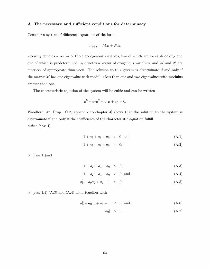
A. The necessary and sufficient conditions for determinacy

Consider a system of difference equations of the form,

zt+1|t =Mzt +Nst,

where zt denotes a vector of three endogenous variables, two of which are forward-looking and

one of which is predetermined, st denotes a vector of exogenous variables, and M and N are

matrices of appropriate dimension. The solution to this system is determinate if and only if

the matrix M has one eigenvalue with modulus less than one and two eigenvalues with modulus

greater than one.

The characteristic equation of the system will be cubic and can be written

µ3 + a2µ2 + a1µ+ a0 = 0.

Woodford [47, Prop. C.2, appendix to chapter 4] shows that the solution to the system is

determinate if and only if the coefficients of the characteristic equation fulfill

either (case I)

1 + a2 + a1 + a0 < 0 and (A.1)

−1 + a2 − a1 + a0 > 0; (A.2)

or (case II)and

1 + a2 + a1 + a0 > 0, (A.3)

−1 + a2 − a1 + a0 < 0 and (A.4)

a20 − a0a2 + a1 − 1 > 0; (A.5)

or (case III) (A.3) and (A.4) hold, together with

a20 − a0a2 + a1 − 1 < 0 and (A.6)

|a2| > 3. (A.7)

64

References

[1] Backus, David, and John Driffill (1986), “The Consistency of Optimal Policy in Stochastic

Rational Expectations Models,” CEPR Discussion Paper No. 124.

[2] Bernanke, Ben, and Michael Woodford (1997), “Inflation Forecasts and Monetary Policy,”

Journal of Money, Credit, and Banking 24, 653—684.

[3] Clarida, Richard, Jordi Galı and Mark Gertler (1998), “Monetary Policy Rules in Practice:

Some International Evidence,” European Economic Review 42, 1033—1067.

[4] Clarida, Richard, Jordi Galı and Mark Gertler (1999), “The Science of Monetary Policy:

A New Keynesian Perspective,” Journal of Economic Literature 37, 1661—1707.

[5] Christiano, Lawrence J., and Christopher J. Gust (1999), “Taylor Rules in a Limited Par-

ticipation Model,” NBER Working Paper No. 7017

[6] Christiano, Lawrence J., and Robert J. Vigfusson (1999), “Maximum Likelihood in the

Frequency Domain: A Time to Build Example,” NBER Working Paper No. 7027

[7] Currie, David, and Paul Levine (1993), Rules, Reputation and Macroeconomic Policy Co-

ordination, Cambridge University Press, Cambridge.

[8] Edge, Rochelle M. (2000), “Time to Build, Time to Plan, Habit Persistence, and the Liquid-

ity Effect,” International Finance Discussion Paper no. 2000-673, Federal Reserve Board,

July.

[9] Floden, Martin (1996), “The Time Inconsistency Problem of Monetary Policy

under Alternative Supply Side Modeling,” Working Paper, Stockholm University,

http://www.hhs.se/personal/floden/.

[10] Giannoni, Marc P. (1999), “Does Model Uncertainty Justify Caution? Robust Optimal

Monetary Policy in a Forward-Looking Model,” Working Paper, Princeton University.

[11] Giannoni, Marc. P., and Michael Woodford (2002), “Optimal Interest-Rate Rules: I. Gen-

eral Theory,” NBER working paper no. 9419, December.

[12] Jonsson, Gunnar (1997), “Monetary Politics and Unemployment Persistence,” Journal of

Monetary Economics 39, 303—325.

65

[13] Judd, John P., and Glenn D. Rudebusch (1998), “Taylor’s Rule and the Fed: 1970-1997,”

FRBSF Economic Review 1998(3), 3—16.

[14] Kerr, William, and Robert J. King (1996), “Limits on Interest Rate Rules in the IS Model,”

Economic Quarterly, Federal Reserve Bank of Richmond, Spring 1996, 47—76.

[15] King, Mervyn A. (1994), “Monetary Policy in the UK,” Fiscal Studies 15, No. 3, 109—128.

[16] King, Mervyn A. (1997), “Changes in UK Monetary Policy: Rules and Discretion in Prac-

tice,” Journal of Monetary Economics 39, 81—97.

[17] King, Mervyn (1997), “The Inflation Target Five Years On,” Bank of England Quarterly

Bulletin 37(4).

[18] Kydland, Finn E., and Edward C. Prescott (1977), “Rules Rather than Discretion: The

Inconsistency of Optimal Plans,” Journal of Political Economy 85, 473—491.

[19] Leeper, Eric M., and Tao Zha (1999), “Identification and Forecasting: Joint Inputs to Policy

Analysis,” Working Paper.

[20] Leitemo, Kai (1999), “Targeting Inflation by Constant-Interest-Rate Forecast,” Working

Paper, Norges Bank.

[21] Levin, Andrew, Wieland, Volker, and John C. Williams (1999), “Robustness of Simple

Monetary Policy Rules under Model Uncertainty,” in Taylor [41].

[22] McCallum, Bennett T. (1981), “Price Level Determinacy with an Interest Rate Policy Rule

and Rational Expectations,” Journal of Monetary Economics 8, 319—329.

[23] McCallum, Bennett T. (1999), “Role of the Minimal State Variable Criterion,” NBER

Working Paper No. 7087.

[24] McCallum, Bennett T. (1997), “Issues in the Design of Monetary Policy Rules,” NBER

Working Paper No. 6016.

[25] Orphanides, Athanasios (1999), “The Quest for Prosperity without Inflation,” Working

Paper, Federal Reserve Board.

[26] Persson, Torsten, and Guido Tabellini (1993), “Designing Institutions for Monetary Stabil-

ity,” Carnegie-Rochester Conference Series on Public Policy 39, 53-84.

66

[27] Rotemberg, Julio J., and Michael Woodford (1997), “An Optimization-Based Econometric

Framework for the Evaluation of Monetary Policy,” NBER Macroeconomics Annual 12,

297—346.

[28] Rotemberg, Julio J., and Michael Woodford (1999), “Interest-Rate Rules in an Estimated

Sticky-Price Model,” in Taylor [41].

[29] Rudebusch, Glenn D., and Lars E.O. Svensson (1999), “Policy Rules for Inflation Target-

ing,” in Taylor [41].

[30] Sargent, Thomas J., and Neil Wallace (1975), “Rational Expectations, the Optimal Mone-

tary Instrument, and the Optimal Money Supply Rule,” Journal of Political Economy 83,

241—254.

[31] Smets, Frank (2000), “What Horizon for Price Stability,” ECB Working Paper No. 24.

[32] Soderlind, Paul (1999), “Solution and Estimation of RE Macromodels with Optimal Policy,”

European Economic Review 43, 813-823.

[33] Svensson, Lars E.O. (1997a), “Inflation Forecast Targeting: Implementing and Monitoring

Inflation Targets,” European Economic Review 41, 1111—1146.

[34] Svensson, Lars E.O. (1997b), “Optimal Inflation targets, ‘Conservative’ Central Banks, and

Linear Inflation Contracts,” American Economic Review 87, 98-114.

[35] Svensson, Lars E.O. (1999a), “How Should Monetary Policy Be Conducted in an Era of

Price Stability?” in New Challenges for Monetary Policy, A Symposium Sponsored by the

Federal Reserve Bank of Kansas City, Jackson Hole, Wyoming, August 26-28, 1999.

[36] Svensson, Lars E.O. (1999b), “Inflation Targeting as a Monetary Policy Rule,” Journal

of Monetary Economics 43, 607-654. Longer working-paper version, including appendix,

available at www.princeton.edu/∼svensson.

[37] Svensson, Lars E.O. (1999c), “Price-Level Targeting vs. Inflation Targeting: A Free Lunch?”

Journal of Money, Credit, and Banking 31, 277-295.

[38] Svensson, Lars E.O. (2003), “What Is Wrong with Taylor Rules? Using Judgment in

Monetary Policy through Targeting Rules,” Journal of Economic Literature, forthcoming.

67

[39] Svensson, Lars E.O., and Michael Woodford (2002), “Indicator Variables for Optimal Pol-

icy,” Journal of Monetary Economics, forthcoming.

[40] Taylor, John B. (1993), “Discretion versus Policy Rules in Practice,” Carnegie-Rochester

Conference Series on Public Policy 39, 195—214.

[41] Taylor, John B., ed. (1999b), Monetary Policy Rules, Chicago University Press.

[42] Vestin, David (1999), “Price-Level Targeting versus Inflation Targeting in a Forward-

Looking Model,” Working Paper, Stockholm University.

[43] Walsh, Carl (1995), “Optimal Contracts for Independent Central Bankers,” American Eco-

nomic Review 85, 150-167.

[44] Woodford, Michael (1999a), “Optimal Monetary Policy Inertia,” NBER Working Paper

No. 7261, July.

[45] Woodford, Michael (1999b), “Commentary: How Should Monetary Policy Be Conducted in

an Era of Price Stability?” in New Challenges for Monetary Policy, A Symposium Sponsored

by the Federal Reserve Bank of Kansas City, Jackson Hole, Wyoming, August 26-28, 1999.

[46] Woodford, Michael (2000), “Pitfalls of Forward-Looking Monetary Policy,” American Eco-

nomic Review Papers and Proceedings 90: 100-104.

[47] Woodford, Michael (2003), Interest and Prices: Foundations of a Theory of Monetary Policy,

forthcoming, Princeton University Press.

[48] Yun, Tack (1996), “Nominal Price Rigidity, Money Supply Endogeneity, and Business Cy-

cles,” Journal of Monetary Economics 37, 345—370.

68