SWIFT-UVOT-CALDB-03-R02Date Original Submitted: 6th April 2006Prepared by: Alex Blustin and Tracey PooleDate Revised: 13th March 2007Revision #02Revised by: Tracey Poole; Alice BreeveldPages Changed: AllComments: Colour correction method adjusted to usein-orbit instrument response curves

SWIFT UVOT CALDB RELEASE NOTESWIFT-UVOT-CALDB-03-R02: COLOUR CORRECTIONS

0. Summary:

The colour corrections describe the relation of UVOT UBV magnitudes tostandard Johnson UBV magnitudes.

1. Component Files:

None.

2. Scope of Document:

This document describes the UVOT-Johnson UBV Colour corrections andhow they have been derived.

3. Changes:

This is the second release of the UBV Colour corrections, replacing firstestimates.In this version the colour correction is derived by simulation using the newin-orbit effective areas (uvot_caldb_effectiveareas_02b.doc) and checkedby comparison with observations. This allows a much wider colour rangeto be used in the analysis.

4. Reason For Update:

An up-date was undertaken to base the colour correction on full spectralsimulations using the in-orbit instrument effective area curves.

5. Expected Updates:

Further updates are expected with updates of the in-orbit effective areacurves.

6. Caveat Emptor:

Due to the lack of faint spectroscopic standard stars, especially in theultraviolet, the effective area curves have been calibrated with very fewstars.

7. Data Used:

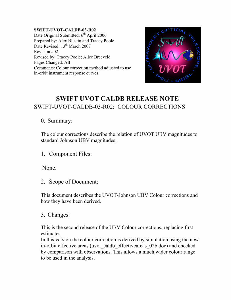
Observations of 9 Landolt stars, 1 white dwarf, with known UBVmagnitudes were used for the optical filter analysis. Where multipleobservations were taken, count rates were calculated for individualexposures and then averaged. Observation details, sorted by observationdate, can be seen in Table 1.

Object Name Filter Date SequenceNumber

Mode ExposureTime(sec)

sa104sw-338 & sa104sw-244 u 22/02/2005 55350004 I 1380.5sa104sw-338 & sa104sw-244 v 22/02/2005 55350004 I 1626.1WD1657+343 v 25/02/2005 55900002 E 605.79sa101-278 & sa101-l3 b 05/03/2005 54950011 I 1523.7sa104sw-338 & sa104sw-244 b 06/03/2005 55350009 I 1155.1PG1525-071B b 07/03/2005 55750005 I 619.0PG1525-071B u 07/03/2005 55750003 I 1327.2PG1525-071B v 07/03/2005 55750001 I 1268.8sa101-278 & sa101-l3 b 09/03/2005 54950005 I 1210.0sa104n-443 & sa104n-457 b 11/03/2005 55400005 I 508.2sa104ne-367 b 11/03/2005 55450003 I 604.5sa95sw-102 u 11/03/2005 54350005 I 569.9sa95sw-102 v 11/03/2005 54350004 I 3706.5

WD1657+343 b 15/03/2005 55900003 I 351.0sa104n-443 & sa104n-457 u 21/03/2005 55400012 I 2025.3sa101-278 & sa101-L3 v 26/03/2005 54950003 I 2661.4sa95sw-102 b 27/03/2005 54350011 I 1649.3sa104ne-367 u 28/03/2005 55450005 I 868.6sa104ne-367 v 05/04/2005 55450008 I 725.9WD1657+343 u 12/04/2005 55900024 I 633.6sa104n-443 & sa104n-457 v 19/04/2005 55400016 I 1128.0WD1657+343 u 14/01/2006 55900035 I 82.6

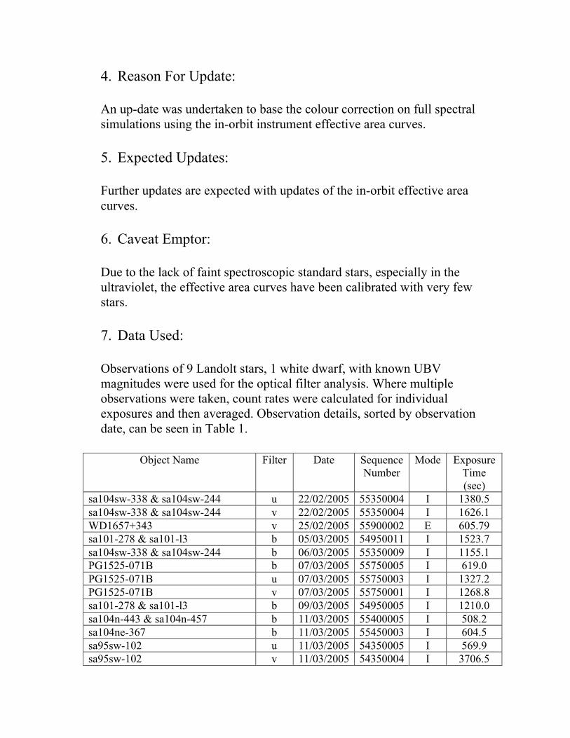
Table 1 - Table containing the observations used to check the colour terms. All of the sequencenumbers in column 4 are missing their first three digits of 000. In column 5, I represents Imagemode, and E represents Event mode.

8. Description of Analysis:

The colour transforms from the UVOT UBV system to the Johnson UBVsystem were calculated using Pickles model spectra (Pickles, 1998, PASP,110, 863), and GRB power law spectral models with power law rangingfrom spectral energy index -2.0 < _ < 0.0, SMC extinction ranging from0.0 < Av < 1.0 and red shift ranging from 0.3 < z < 2.0, see Figure 1 for anexample.

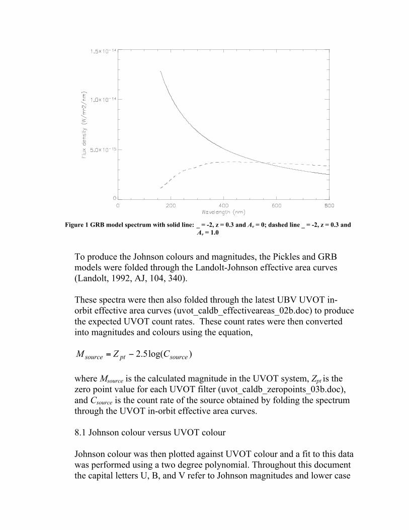
Figure 1 GRB model spectrum with solid line: _ = -2, z = 0.3 and Av = 0; dashed line _ = -2, z = 0.3 andAv = 1.0

To produce the Johnson colours and magnitudes, the Pickles and GRBmodels were folded through the Landolt-Johnson effective area curves(Landolt, 1992, AJ, 104, 340).

These spectra were then also folded through the latest UBV UVOT in-orbit effective area curves (uvot_caldb_effectiveareas_02b.doc) to producethe expected UVOT count rates. These count rates were then convertedinto magnitudes and colours using the equation,

)log(5.2 sourceptsource CZM −=

where Msource is the calculated magnitude in the UVOT system, Zpt is thezero point value for each UVOT filter (uvot_caldb_zeropoints_03b.doc),and Csource is the count rate of the source obtained by folding the spectrumthrough the UVOT in-orbit effective area curves.

8.1 Johnson colour versus UVOT colour

Johnson colour was then plotted against UVOT colour and a fit to this datawas performed using a two degree polynomial. Throughout this documentthe capital letters U, B, and V refer to Johnson magnitudes and lower case

letters u, b, and v refer to UVOT magnitudes. Figure 2 shows the resultsof this fit to the data for U-B versus u-b (top plot), B-V versus b-v (middleplot) and U-V versus u-v (bottom plot). The blue solid line in each plotshows the best polynomial fit to the pickles data, the solid green line ineach plot shows the best polynomial fit to the GRB models data, and thered solid line shows x=y. The residuals to the fits are shown in the lowerpanel of each plot, and show good agreement to within 0.05 magnitudes,apart from a few outliers. The black points represent the Pickles stars andthe green points represent the GRB models.

These simulated fits were then checked using observations. Figure 3 plotsthe Johnson and UVOT colours of the observed Landolt stars used for zeropoint analysis (see uvot_caldb_zeropoints_03b.doc for details on theanalysis of these stars). This figure shows that within the scatter of theseobservations, the fits produced with the Pickles stars agree with theobservations.

The colour terms given from the polynomial fits with the Pickles stars areas follows:

U−B = 0.034[±0.007] + 0.862[±0.007](u−b) + 0.055[±0.006](u−b)2

−1.482 < u−b < 1.871RMS error on the fit: 0.0573 mag

B−V = − 0.004[±0.004] + 1.039[±0.011](b−v) - 0.037[±0.007](b−v)2

−0.364 < b−v < 1.935RMS error on the fit: 0.0253 mag

U−V = 0.071[±0.010] + 0.899[±0.008](u−v) + 0.018[±0.003](u−v)2

−1.846 < u−v < 3.558RMS error on the fit: 0.0752 mag

The colour terms given from the polynomial fits with the GRB models areas follows:

U−B = 0.086[±0.003] + 0.886[±0.007](u−b) + 0.050[±0.006](u−b)2

−1.380 < u−b < 0.543RMS error on the fit: 0.0775 mag

B−V = − 0.008[±0.001] + 1.012[±0.003](b−v) - 0.018[±0.002](b−v)2

−0.124 < b−v < 1.483RMS error on the fit: 0.0342 mag

U−V = 0.162[±0.002] + 0.904[±0.002](u−v) + 0.010[±0.002](u−v)2

−1.505 < u−v < 2.026RMS error on the fit: 0.1017 mag

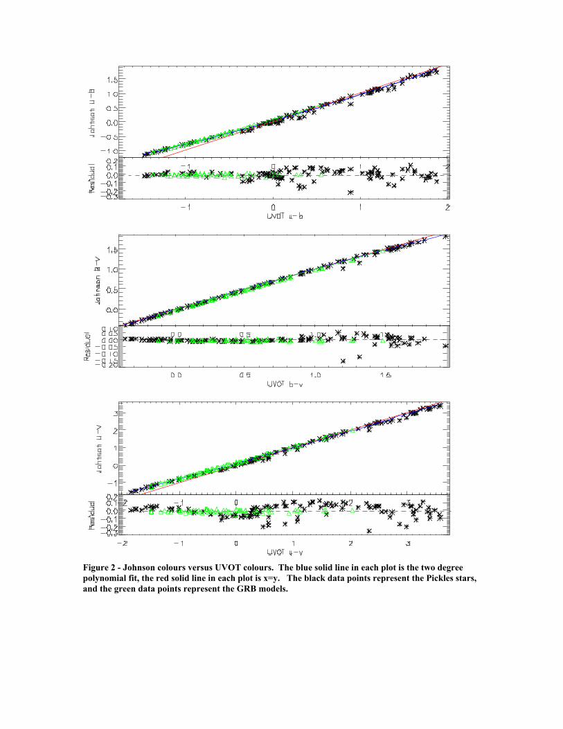
Figure 2 - Johnson colours versus UVOT colours. The blue solid line in each plot is the two degreepolynomial fit, the red solid line in each plot is x=y. The black data points represent the Pickles stars,and the green data points represent the GRB models.

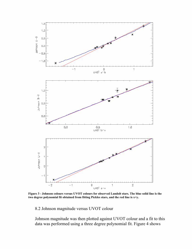
Figure 3 - Johnson colours versus UVOT colours for observed Landolt stars. The blue solid line is thetwo degree polynomial fit obtained from fitting Pickles stars, and the red line is x=y.

8.2 Johnson magnitude versus UVOT colour

Johnson magnitude was then plotted against UVOT colour and a fit to thisdata was performed using a three degree polynomial fit. Figure 4 shows

the results of this fit to the data for B-v versus b-v (top left plot), B-bversus u-b (top right panel), V-v versus b-v (middle left plot), V-v versusu-v (middle right plot), U-u versus u-b (bottom left plot), and U-u versusu-v (bottom right plot). The blue solid line in each plot shows the bestpolynomial fit to the data. The residuals to this fits are shown in the lowerpanel of each plot (black data points), and show good agreement to within0.05 magnitudes. The black points represent the Pickles stars and the greenpoints represent the GRB models. Figure 4 shows that the Pickles starsand the GRB models do not follow the same fit, therefore a two degreepolynomial fit was performed on the GRB model data, which can be seenas the red solid line in Figure 4. Again, the residuals to the GRB fit (greendata points) are shown in the lower panel of each plot, and show goodagreement to within 0.05 magnitudes.

These simulated fits were checked using observations. Figure 5 plots theJohnson and UVOT colours of the observed Landolt stars used for zeropoint analysis (see uvot_caldb_zeropoints_03b.doc for details on analysisof these stars). This figure shows that within the scatter of theseobservations, the fits produced with the Pickles stars agree withobservations.

The colour terms given from the polynomial fits for the pickles stars are asfollows:

B−b = 0.021[±0.003] + 0.005[±0.012](b−v) − 0.014[±0.022](b−v)2 − 0.011[±0.010](b−v)3

−0.364 < b−v < 1.935RMS error on the fit: 0.0203 mag

B−b = 0.011[±0.004] − 0.011[±0.008](u−b) − 0.008[±0.004](u−b)2 − 0.002[±0.004](u−b)3

−1.482 < u−b < 1.871RMS error on the fit: 0.0295 mag

V−v = 0.029[±0.002] − 0.009[±0.009](b−v) − 0.037[±0.016](b−v)2 + 0.017[±0.007](b−v)3

−0.364 < b−v < 1.935RMS error on the fit: 0.0144 mag

V−v = 0.026[±0.002]−0.014[±0.002](u−v) − 0.005[±0.001](u−v)2 + 0.002[±0.0005](u−v)3

−1.846 < u−v < 3.558RMS error on the fit: 0.0146 mag

U−u = 0.042[±0.010] − 0.130[±0.020](u−b) + 0.053[±0.010](u−b)2 − 0.013[±0.010](u−b)3

−1.482 < u−b < 1.871RMS error on the fit: 0.0732 mag

U−u = 0.069[±0.012] − 0.093[±0.009](u−v) + 0.037[±0.007](u−v)2 − 0.007[±0.002](u−v)3

−1.846 < u−v < 3.558RMS error on the fit: 0.0712 mag

The colour terms given from the polynomial fits for the GRB models areas follows:

B−b = 0.016[±0.0003] − 0.009[±0.001](b−v) − 0.023[±0.001](b−v)2

−0.124 < b−v < 1.483RMS error on the fit: 0.0012 mag

B−b = −0.018[±0.0005] − 0.045[±0.001](u−b) − 0.014[±0.001](u−b)2 −1.380 < u−b < 0.543RMS error on the fit: 0.0019 mag

V−v = 0.023[±0.001] − 0.021[±0.003](b−v) − 0.005[±0.003](b−v)2

−0.124 < b−v < 1.483RMS error on the fit: 0.0036 mag

V−v = 0.010[±0.0007] − 0.012[±0.0006](u−v) − 0.0009[±0.0006](u−v)2

−1.505 < u−v < 2.026RMS error on the fit: 0.0039 mag

U−u = 0.068[±0.003] − 0.159[±0.007](u−b) + 0.036[±0.006](u−b)2

−1.380 < u−b < 0.543RMS error on the fit: 0.0111 mag

U−u = 0.172[±0.002] − 0.108[±0.002](u−v) + 0.009[±0.002](u−v)2

−1.505 < u−v < 2.026RMS error on the fit: 0.0124 mag

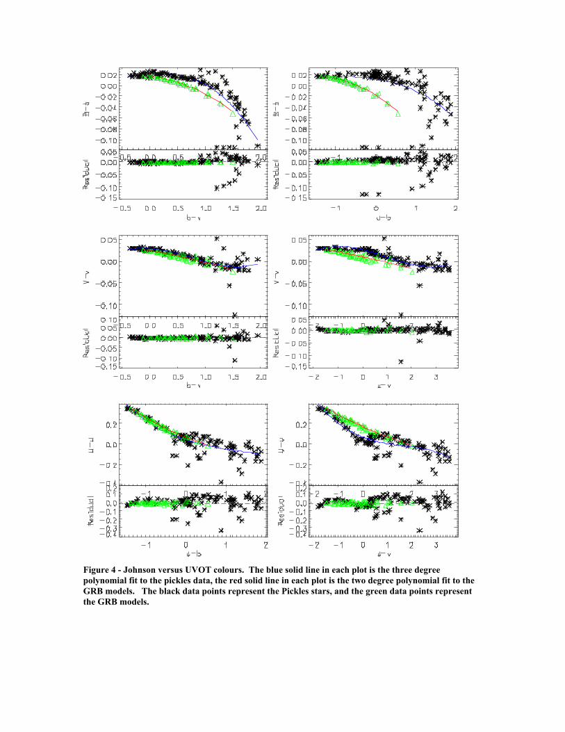
Figure 4 - Johnson versus UVOT colours. The blue solid line in each plot is the three degreepolynomial fit to the pickles data, the red solid line in each plot is the two degree polynomial fit to theGRB models. The black data points represent the Pickles stars, and the green data points representthe GRB models.

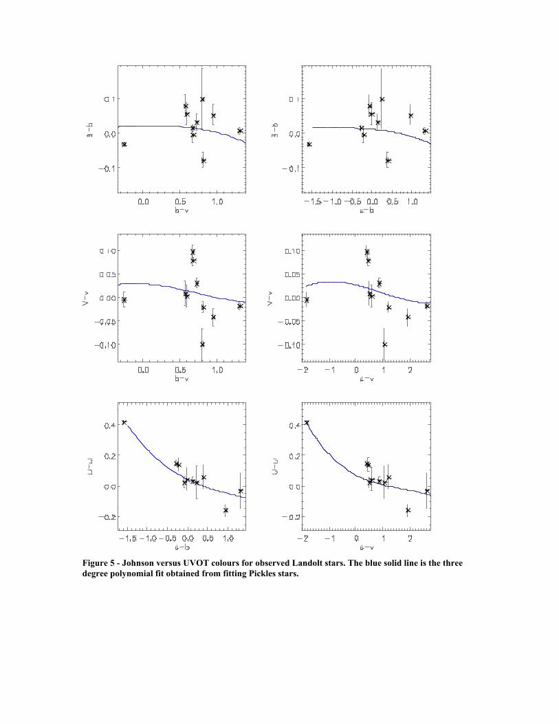
Figure 5 - Johnson versus UVOT colours for observed Landolt stars. The blue solid line is the threedegree polynomial fit obtained from fitting Pickles stars.