Embed Size (px)
Citation preview
Shift dynamics modelling foroptimization of variator slip control ina continuously variable transmission
S.W.H.Simons
DCT Report 2006-081Technische Universiteit Eindhoven
Master of Science Thesis
Committee: ir. T. W. G. L. Klaassen† (Coach)dr. P. A. Veenhuizen†dr. ir. A. A. H. Damen‡prof. dr. ir. M. Steinbuch†
†Eindhoven University of TechnologyDepartment of Mechanical EngineeringSection Control Systems Technology, Automotive Engineering Science
‡Eindhoven University of TechnologyDepartment of Electrical EngineeringSection Measurement and Control Systems, Control Systems
Eindhoven, 3rd July 2006

Samenvatting
Steeds meer duwband Continu Variabele Transmissies (CVT) worden geïmplementeerd, vanwegehun ongeëvenaarde schakel gemak. Een hoge overdrive ratio zorgt voor lagere motor snelheid,verbeterd rijcomfort op snelwegen en een gereduceerd brandstof gebruik. Doordat de 6 of 7 trapsautomatische versnellingsbakken echter steeds meer concurrerend worden, is het erg belangrijkde prestaties van de CVT te verbeteren. Met name op het gebied van efficiëntie, robuustheid enkoppel capaciteit. Efficiëntie verbetering, door middel van het reduceren van knijpkrachten in devariator tot een minimal niveau, heeft zich bewezen. Door het reduceren van de knijpkrachten kande variator in zijn meest efficiënte werkpunt opereren. Ook wordt de mechanische belasting op devariator geminimaliseerd en worden de hydraulische actuatie verliezen teruggebracht.
De CVT slip regeling techniek, zorgt voor de best mogelijk efficiëntie, in combinatie met verbe-terde robuustheid ten opzichte van schade als gevolg van slip. Terwijl voorafgaande onderzoekenzich voornamelijk bezig hielden met de dynamica tijdens stationair rijgedrag, bleek dat tijdenssnel schakelen andere dynamische effecten optreden. Hiervoor zijn theoretische schakel model-len gevalideerd en met elkaar vergeleken. Het beste model is gebruikt voor de optimalisatie vande huidige slip regeling. Hiervoor is een slip regeling ontworpen op basis van Linear QuadraticGaussian (LQG) control. Tevens is een PI regeling voor de ratio van de CVT variator ontworpen.Experimenten in een test voertuig zijn gebruikt om de regeling te valideren en te vergelijken methet ontwerp voor de slip regeling uit vorige onderzoeken.
i

ii
Abstract
V-belt type Continuously Variable Transmissions (CVT) are applied in an increasing number ofvehicles as a result of their unparalleled shift comfort. Large ratio coverage allows for reducedengine speed, improved highway driving comfort and reduced fuel consumption. With the adventof the competing automatic transmissions with 6 or even 7 steps, it becomes increasingly impor-tant to further improve the performance in terms of efficiency, robustness and torque capacityof the CVT. Improvements on the efficiency of the pushbelt CVT by reducing variator clampingforces to minimum values are well established. By reducing clamping forces such that the variatoroperates in its most efficient point, the mechanical load on this variator is minimized and hydraulicactuation losses are reduced.
The CVT slip control technique allows for best possible transmission efficiency, combined withimproved robustness for slip damage. However, CVT slip dynamics during transient behaviourcould not be neglected compared to steady state behaviour. Theoretical CVT shifting models arevalidated and compared to best agreement with experimental results. The results are used formodel optimization. A Linear Quadratic Gaussian (LQG) controller is designed for the CVT slipcontrol, as well as a Proportional Integral (PI) controller for CVT ratio control. Experimentalresults in a test vehicle prove validity and compare the design with the previous work on thisapproach.
iii

iv
Contents
Samenvatting i
Abstract iii
Nomenclature and acronyms vii
1 Introduction 1
2 Variator slip control 32.1 Variator slip and functional properties . . . . . . . . . . . . . . . . . . . . . . . . . 32.2 Vehicle implementation previous slip controller . . . . . . . . . . . . . . . . . . . . 5
2.2.1 Experimental vehicle . . . . . . . . . . . . . . . . . . . . . . . . . . . . . . . 52.2.2 Analysis previous slip controller . . . . . . . . . . . . . . . . . . . . . . . . . 6
3 Transient pushbelt variator models 93.1 Literature on shifting mechanisms . . . . . . . . . . . . . . . . . . . . . . . . . . . 93.2 Transient models . . . . . . . . . . . . . . . . . . . . . . . . . . . . . . . . . . . . . 11
3.2.1 Ide’s model . . . . . . . . . . . . . . . . . . . . . . . . . . . . . . . . . . . . 113.2.2 CMM model . . . . . . . . . . . . . . . . . . . . . . . . . . . . . . . . . . . 11
3.3 Pulley thrust ratio . . . . . . . . . . . . . . . . . . . . . . . . . . . . . . . . . . . . 123.4 Validation and comparison of transient models . . . . . . . . . . . . . . . . . . . . 13
4 Modeling system dynamics 174.1 Variator dynamics . . . . . . . . . . . . . . . . . . . . . . . . . . . . . . . . . . . . 174.2 Actuation system dynamics . . . . . . . . . . . . . . . . . . . . . . . . . . . . . . . 19
4.2.1 Clamping force actuation . . . . . . . . . . . . . . . . . . . . . . . . . . . . 194.2.2 Shifting force actuation . . . . . . . . . . . . . . . . . . . . . . . . . . . . . 21
4.3 Linear CVT model . . . . . . . . . . . . . . . . . . . . . . . . . . . . . . . . . . . . 244.4 Interaction analysis . . . . . . . . . . . . . . . . . . . . . . . . . . . . . . . . . . . . 25
5 Control design and strategy 275.1 Ratio control . . . . . . . . . . . . . . . . . . . . . . . . . . . . . . . . . . . . . . . 275.2 Slip control . . . . . . . . . . . . . . . . . . . . . . . . . . . . . . . . . . . . . . . . 29
5.2.1 LQG feedback control . . . . . . . . . . . . . . . . . . . . . . . . . . . . . . 305.2.2 Feedforward control . . . . . . . . . . . . . . . . . . . . . . . . . . . . . . . 325.2.3 Slip control strategy . . . . . . . . . . . . . . . . . . . . . . . . . . . . . . . 32
5.3 Control implementation in test-vehicle . . . . . . . . . . . . . . . . . . . . . . . . . 335.3.1 Torque converter control . . . . . . . . . . . . . . . . . . . . . . . . . . . . . 335.3.2 Safety measures . . . . . . . . . . . . . . . . . . . . . . . . . . . . . . . . . . 33
6 Implementation results 356.1 Simulation results . . . . . . . . . . . . . . . . . . . . . . . . . . . . . . . . . . . . 356.2 Vehicle implementation results . . . . . . . . . . . . . . . . . . . . . . . . . . . . . 36
v
vi CONTENTS
7 Conclusions and recommendations 417.1 Conclusions . . . . . . . . . . . . . . . . . . . . . . . . . . . . . . . . . . . . . . . . 417.2 Recommendations . . . . . . . . . . . . . . . . . . . . . . . . . . . . . . . . . . . . 41
Bibliography 42
A Jatco CKkai-CVT 45
B Nissan Primera test vehicle 47
C Shift speed experiments 51
D Pulley thrust ratio 55
E Dimensional analysis 59
F CMM model 61
G Linearized model 63
H Electro-hydraulic system 65
I Linearizing shift valve model 67
J Ratio control analysis 69
K Non-linear model 71
L Chassis dyno 75
Nomenclature and acronyms
NomenclatureSymbol Description Value [Unit]Acar frontal area of the vehicle 1.8 [m2]Ap Primary cylinder surface [m2]As Secondary cylinder surface [m2]Av Shift valve orifice [m2]Fair Air drag [N]Fgrad Gradient resistance [N]Fp Primary clamping force [N]F ∗
p Primary clamping force at steady state conditions [N]Frol Rolling resistance [N]Fs Secondary clamping force [N]Fspr,0 Preload spring secondary moveable pulley [N]Ir Integral gain for ratio control [-]Je Engine side or primary inertia 0.356 [kgm2]Js Vehicle side or secondary inertia 4.96 [kgm2]Kstep Axial movement spindle pro step of the stepper motor 1.05 ·10−3 [m]L Belt length 0.703 [m]Pr Proportional gain for ratio control [-]Rp Primary running radius [m]Rs Secondary running radius [m]Sf Safety factor [-]Td Road load torque [Nm]Te Engine torque [Nm]Tp Primary pulley belt torque [Nm]Tpump,loss Torque losses at the oil pump [Nm]Trl Road load torque [Nm]Ts Secondary pulley belt torque [Nm]Tvar,loss Variator torque losses [Nm]Vp0 Initial primary cylinder volume 10−4 [m3]a Axial pulleys distance 0.168 [m]
vii
viii CONTENTS
cf Discharge coefficient 0.6 [-]cpl Primary leak coefficient 0.6 [-]cw Air drag coefficient 0.34 [-]fcp Centrifugal coefficient primary pulley 5.4 ·10−3
[Ns2/rad]fcs Centrifugal coefficient secondary pulley 4.5 ·10−2
[Ns2/rad]fr Rolling resistance coefficient 0.012 [-]g Gravitational constant 9.81 [m/s2]kc Constant in the CMM model for rate of ratio changing [-]kc,x Constant in the CMM model for axial primary pulley speed [-]ki Constant in Ide’s model [-]koil Oil compressibility 5·10−9 [m2/N]kspr Spring constant secondary pulley [N/m]mi Constants in pulley thrust ratio approximation [-]mcar Simulated vehicle mass 1300 [kg]np Primary pulley rotational speed [rpm]pd Drain pressure ·104 [Pa]pp Primary pulley pressure [Pa]p∗p Primary pulley pressure at steady state conditions [Pa]pp0 Minimal primary pulley pressure [Pa]pph Primary pulley pressure at turning point between slip and creep
mode[Pa]
pp,ss Primary pulley pressure at steady state [Pa]pp,val Primary pulley pressure due to shift valve position operation [Pa]ps Secondary pulley pressure [Pa]rfd Final drive 0.1827 [-]rg Geometric ratio [-]rs Speed ratio [-]rs0 Speed ratio at no load conditions [-]usol Solenoid input [-]ustep Stepper motor input [-]xp Axial position primary pulley [m]xp,min Minimal axial position primary pulley 1.31·10−2 [m]xp,ref Axial position reference [m]xs Axial position secondary pulley [m]xs,max Maximal axial position secondary pulley 3.08·10−2 [m]xstep Stepper motor position [m]xv Valve position [m]∆F Absolute shifting force [N]∆ln F Logarithm relative shifting force [-]∆pi Pressure drop over the shift valve [bar]Λ Relative gain array [-]∆β Maximum amplitude of the wedge half-angle variations along the
contact arc[-]
CONTENTS ix
Ψ Pulley thrust ratio [-]α Gradient of the road []β Pulley wedge angle 11 []β∗ Pulley wedge angle at loaded conditions []γ Throttle position [%]η Efficiency [%]κ Interaction measure [-]λ Relative gain array element [-]µ Traction coefficient 0.09 [-]µeff Effective traction coefficient [-]ν Relative belt slip [-]νref Relative belt slip reference [-]ρair Air density 1.29 [kg/m3]ρoil ATF oil density (at 80 C) 8.3 ·102[kg/m3]τ Torque ratio [-]ωe Engine rotational speed [rad/s]ωp Primary pulley rotational speed [rad/s]ωs Secondary pulley rotational speed [rad/s]
AcronymsSymbol DescriptionATF Automatic Transmission FluidCAN Controller Area NetworkCMM Carbone Mangialardi MantriotaCV T Continuously Variable TransmissionECM Engine Control ModuleLOW Low ratio (rg = 0.43)LQG Linear Quadratic GaussianLV DT Linear Variable Displacement TransducerMIMO Multiple Input Multiple OutputMED Medium ratio (rg = 1)OD Overdrive ratio (rg = 2.15)PI Proportional IntegralPLTR Power Loop Test RigPWM Pulse Width ModulationRGA Relative Gain ArraySISO Single Input Single OutputTCM Transmission Control ModuleV DT Van Doorne’s Transmissie

x CONTENTS
Chapter 1
Introduction
The low efficiency in a present production CVT is to a large extent caused by high clamping forcelevels. To prevent major slip events between pulleys and belt, the clamping forces are much higherthan necessary for proper operation. These higher forces result in higher torque losses in the vari-ator. Additionally, higher clamping forces require higher hydraulic pressures, thereby leading toincreased pumping losses. Previous studies have shown that reducing these clamping forces resultin a remarkable increase in efficiency [1]. However, the risk of belt slip is increased, using theselow clamping forces. Present work by Van Drogen and Van der Laan [23] has shown that belt slipis allowed to a certain extent. Bonsen et al. [1] have demonstrated a possible efficiency gain byusing slip control instead of the conventional control strategy.
In earlier studies, conditions for optimum performance regarding efficiency and robustness wereidentified and validated for steady state conditions. However, stability robustness during ratiochanges proved to be insufficient during tests in an experimental vehicle [1].
To deal with CVT slip dynamics during transient behaviour, a theoretical model is necessary.In this report, a novel CVT shifting model, recently proposed by Carbone et al. [7], is testedexperimentally and compared with the model of Ide et al. [9]. The relationship between theclamping forces acting on the moveable pulley sheave, the rate of change of speed ratio, the load-ing conditions and the belt velocity are investigated both from a theoretical and an experimentalpoint of view. Experiments are carried out on a test rig and in a test vehicle.
The main goal of this report is to propose a variator control strategy, which achieves increasedrobustness and drivability compared to the control strategy proposed and implemented by Bonsenet al. [1].
To achieve this goal, first the basic principles of slip behaviour in the pushbelt variator are de-scribed. Also in Chapter 2, the previous designed slip controller is analysed. Especially the fastshifting events, where failure of the previous slip controller occurred, are investigated to improveslip control robustness. To get more insight in shifting behaviour of the CVT, a short literaturestudy is given in Chapter 3. Subsequently, the obtained models are validated and compared. Thisleads to the model, which gives the best prediction of the CVT’s dynamical behaviour during shift-ing manoeuvres for given values of the applied clamping forces, torque load and pulley angularvelocity. In Chapter 4 the dynamic model of the variator, including actuation system, is derived.The model makes use of the CVT slip and shifting dynamics, which are obtained in the previouschapters. The interaction of the derived plant is analysed for control design possibilities. Thedesigned controllers, for both slip and ratio control are described in Chapter 5. For slip control,a design based on LQG control is proposed. The obtained controllers are tested in a experimen-tal vehicle and compared with the previous proposed gain scheduled PI controller in Chapter 6.Finally, in Chapter 7 conclusions and recommendations are given.
1

2 CHAPTER 1. INTRODUCTION
Chapter 2
Variator slip control
Bonsen et al. [1] presents the possible efficiency gain by using slip control instead of the conven-tional strategy. This controller is based on the slip between pulleys and pushbelt in a CVT. Thisrelative slip and its functional properties are defined in the next section. Afterwards the previousslip controller, proposed by Bonsen et al. [1], is discussed and analysed.
2.1 Variator slip and functional propertiesThe theory of the slip controller is based on the power transfer in the CVT, which is due to thefriction between pulleys and pushbelt. For a pushbelt variator, the relation between secondaryclamping force Fs and input torque Tp can be represented by the effective friction coefficient
µeff (ν, rg) =Tp cos β
2FsRp(2.1)
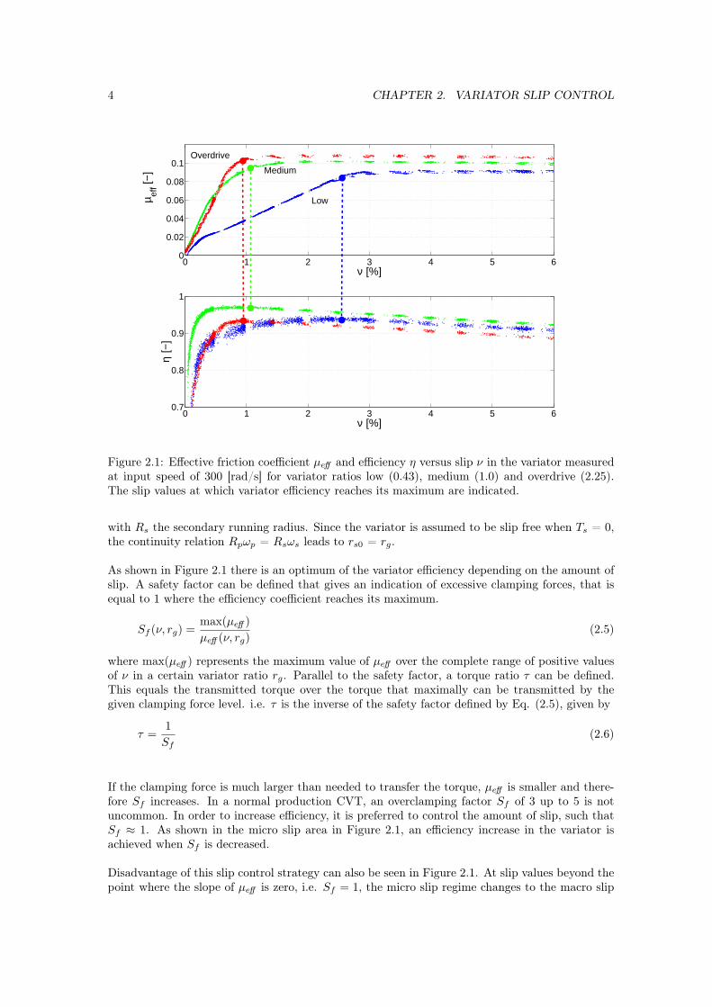
where Rp denotes the running radius of belt on the primary pulley and β denotes the pulleywedge angle. Experiments have shown that this µeff depends strongly on the CVT ratio rg andthe amount of slip ν between belt and pulleys, but only weakly on clamping force and shaft speed.The dependency between slip and µeff at fixed ratio and secondary clamping force is shown in theupper part of Figure 2.1. The traction increases linearly with slip until a maximum is reachedat 1 [%] to 3 [%]. At higher slip levels, the traction decreases slowly with slip. A distinctionbetween a stable micro-slip area and a unstable macro-slip area can be made. The turning pointbetween these regimes is at the highest possible effective friction coefficient. Close to this turn-ing point the maximum variator efficiency can be reached, as shown in the lower part of Figure 2.1.
In this study the relative slip ν is defined as
ν = 1− rs
rs0(2.2)
where rs is the speed ratio and rs0 the speed ratio at no load conditions, assuming that there isno slip when the secondary shaft is unloaded, i.e. Ts = 0. The speed ratio rs is defined as
rs =ωs
ωp(2.3)
where ωp and ωs represent the primary and secondary rotational pulley speed, respectively. Assum-ing the belt runs on perfectly circular paths on the wrapped angles of both pulleys, the geometricratio rg can be defined by
rg =Rp
Rs(2.4)
3
4 CHAPTER 2. VARIATOR SLIP CONTROL
0 1 2 3 4 5 60
0.02
0.04
0.06
0.08
0.1
ν [%]
µ eff [−
]
0 1 2 3 4 5 60.7
0.8
0.9
1
ν [%]
η [−
]Medium
Low
Overdrive
Figure 2.1: Effective friction coefficient µeff and efficiency η versus slip ν in the variator measuredat input speed of 300 [rad/s] for variator ratios low (0.43), medium (1.0) and overdrive (2.25).The slip values at which variator efficiency reaches its maximum are indicated.
with Rs the secondary running radius. Since the variator is assumed to be slip free when Ts = 0,the continuity relation Rpωp = Rsωs leads to rs0 = rg.
As shown in Figure 2.1 there is an optimum of the variator efficiency depending on the amount ofslip. A safety factor can be defined that gives an indication of excessive clamping forces, that isequal to 1 where the efficiency coefficient reaches its maximum.
Sf (ν, rg) =max(µeff )µeff (ν, rg)
(2.5)
where max(µeff ) represents the maximum value of µeff over the complete range of positive valuesof ν in a certain variator ratio rg. Parallel to the safety factor, a torque ratio τ can be defined.This equals the transmitted torque over the torque that maximally can be transmitted by thegiven clamping force level. i.e. τ is the inverse of the safety factor defined by Eq. (2.5), given by
τ =1Sf
(2.6)
If the clamping force is much larger than needed to transfer the torque, µeff is smaller and there-fore Sf increases. In a normal production CVT, an overclamping factor Sf of 3 up to 5 is notuncommon. In order to increase efficiency, it is preferred to control the amount of slip, such thatSf ≈ 1. As shown in the micro slip area in Figure 2.1, an efficiency increase in the variator isachieved when Sf is decreased.
Disadvantage of this slip control strategy can also be seen in Figure 2.1. At slip values beyond thepoint where the slope of µeff is zero, i.e. Sf = 1, the micro slip regime changes to the macro slip
2.2. VEHICLE IMPLEMENTATION PREVIOUS SLIP CONTROLLER 5
regime as also indicated in [23]. This macro slip area is unstable and slip could increase rapidlydue to driveline disturbances. Limited excursions into this area may however be allowed for thepushbelt variator.
At steady state operation points with small disturbances, the present slip control achieved goodresults as indicated in [1]. Furthermore, disturbances by shock loads due to full throttle andemergency braking were overcome by a predictive feedforward, guaranteeing robustness in mostoperating points. However during fast shifting actions, in combination with load peaks due toengine torque and inertias, major slip events occurred. Therefore shifting behaviour is taken intoaccount in the slip model as described in Chapter 4.
2.2 Vehicle implementation previous slip controller
Experiments on test rigs by Pulles [16] showed that the strategy to control slip had great potentialfor efficiency improvement, while remaining robustness in a production CVT. For more realisticexperiments, especially with regard to robustness due to high and unpredictable loads disturbances,the previous slip controller proposed by Bonsen et al. [1] is implemented in a production car.
2.2.1 Experimental vehicle
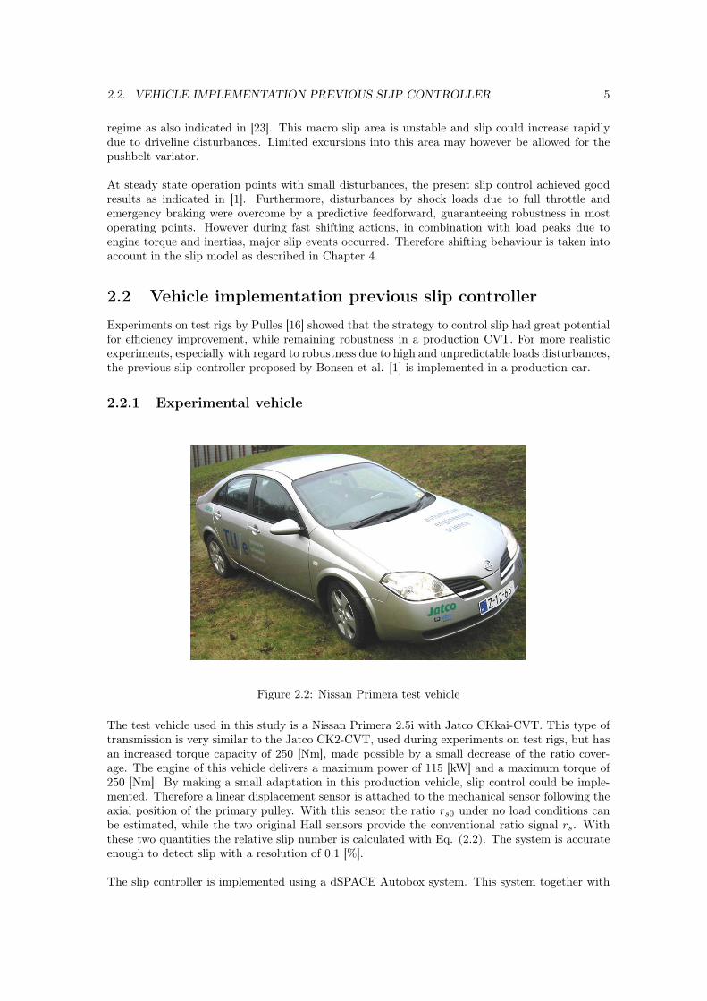
Figure 2.2: Nissan Primera test vehicle
The test vehicle used in this study is a Nissan Primera 2.5i with Jatco CKkai-CVT. This type oftransmission is very similar to the Jatco CK2-CVT, used during experiments on test rigs, but hasan increased torque capacity of 250 [Nm], made possible by a small decrease of the ratio cover-age. The engine of this vehicle delivers a maximum power of 115 [kW] and a maximum torque of250 [Nm]. By making a small adaptation in this production vehicle, slip control could be imple-mented. Therefore a linear displacement sensor is attached to the mechanical sensor following theaxial position of the primary pulley. With this sensor the ratio rs0 under no load conditions canbe estimated, while the two original Hall sensors provide the conventional ratio signal rs. Withthese two quantities the relative slip number is calculated with Eq. (2.2). The system is accurateenough to detect slip with a resolution of 0.1 [%].
The slip controller is implemented using a dSPACE Autobox system. This system together with
6 CHAPTER 2. VARIATOR SLIP CONTROL
a signal conditioning box provides the measurement data of the transmission during experiments.The setup of the system can be seen in Appendix B. Furthermore, the three actuation signals of thehydraulic system of the CVT can be controlled. These are the Pulse Width Modulation (PWM)signals for the line pressure and torque converter lockup clutch and the stepper motor controlsignal. In the previous slip controller torque converter lockup and ratio control were preformedby the original TCM (Transmission Control Module).
2.2.2 Analysis previous slip controllerThe previous slip controller consists of a gain scheduled proportional integral (PI) controller andfeedforward. The parameters of the PI controller vary, depending on the CVT ratio and betweenthe micro- and macro regime, as obtained by Pulles [16]. The feedforward is needed becausethe bandwidth of the slip controller is not sufficient to compensate for the fast dynamics of acombustion engine, due to the delay in the hydraulic circuits. This feedforward is based on theminimal clamping force necessary to transmit the engine torque Te, as shown in Eq. (2.7).
Fs,FFW =Te(ωe, γ) cos β
2Rp max(µeff )(2.7)
The engine torque Te is estimated using a engine map, dependent on throttle position γ and en-gine speed ωe. Moreover, fast increase of the throttle position requires fast downshifts. This incombination with torque peaks induced by engine and accelerations in the variator, can trigger slippeaks. Therefore, an additional compensation in the feedforward is necessary. This compensationincreases the minimal clamping force with a safety factor, if the derivative of the throttle positionexceeds 80 [%/s]. This increase is maintained for 2.5 [s]. The amount of this safety depends onthe maximum amount of the derivative during a throttle position increase.
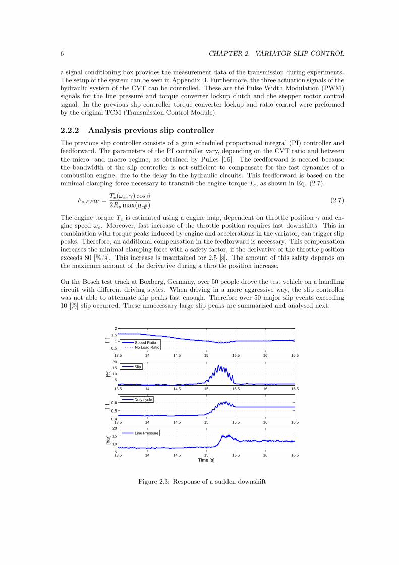
On the Bosch test track at Boxberg, Germany, over 50 people drove the test vehicle on a handlingcircuit with different driving styles. When driving in a more aggressive way, the slip controllerwas not able to attenuate slip peaks fast enough. Therefore over 50 major slip events exceeding10 [%] slip occurred. These unnecessary large slip peaks are summarized and analysed next.
13.5 14 14.5 15 15.5 16 16.5
0.5
1
1.5
2
[−]
Speed RatioNo Load Ratio
13.5 14 14.5 15 15.5 16 16.5
5
10
15
20
[%]
Slip
13.5 14 14.5 15 15.5 16 16.50.4
0.5
0.6
[−]
Duty cycle
13.5 14 14.5 15 15.5 16 16.55
10
15
20
Time [s]
[bar
]
Line Pressure
Figure 2.3: Response of a sudden downshift
2.2. VEHICLE IMPLEMENTATION PREVIOUS SLIP CONTROLLER 7
In spite of the precautions during fast throttle increase and sudden downshifts, not all slip peakscaused by this event could be prevented. An example is shown in Figure 2.3. During downshiftthe primary pressure drops and therefore torque capacity of the variator decreases, while due toinertias, transferable torque increases. This causes an increase in slip. Bad implementation ofthe safety increase for fast throttle position increase, gave sudden drops in the duty cycle duringdownshifting. This triggered slip peaks instead of preventing them.
0.5 1 1.5 2 2.5 3 3.50.5
1
1.5
2
[−]
Speed RatioNo Load Ratio
0.5 1 1.5 2 2.5 3 3.50
5
10
15
[%]
Slip
0.5 1 1.5 2 2.5 3 3.50.5
0.6
0.7
[−]
Duty cycle
0.5 1 1.5 2 2.5 3 3.5
10
15
20
Time [s]
[bar
]
Line Pressure
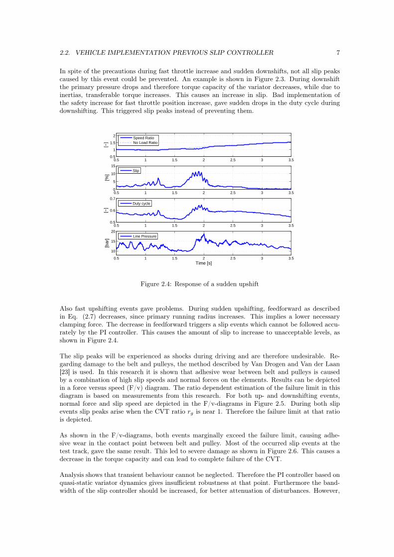
Figure 2.4: Response of a sudden upshift
Also fast upshifting events gave problems. During sudden upshifting, feedforward as describedin Eq. (2.7) decreases, since primary running radius increases. This implies a lower necessaryclamping force. The decrease in feedforward triggers a slip events which cannot be followed accu-rately by the PI controller. This causes the amount of slip to increase to unacceptable levels, asshown in Figure 2.4.
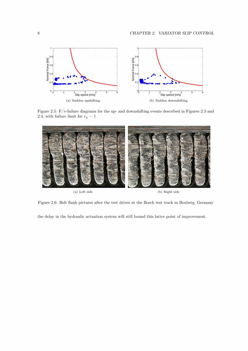
The slip peaks will be experienced as shocks during driving and are therefore undesirable. Re-garding damage to the belt and pulleys, the method described by Van Drogen and Van der Laan[23] is used. In this research it is shown that adhesive wear between belt and pulleys is causedby a combination of high slip speeds and normal forces on the elements. Results can be depictedin a force versus speed (F/v) diagram. The ratio dependent estimation of the failure limit in thisdiagram is based on measurements from this research. For both up- and downshifting events,normal force and slip speed are depicted in the F/v-diagrams in Figure 2.5. During both slipevents slip peaks arise when the CVT ratio rg is near 1. Therefore the failure limit at that ratiois depicted.
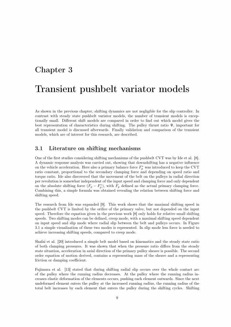
As shown in the F/v-diagrams, both events marginally exceed the failure limit, causing adhe-sive wear in the contact point between belt and pulley. Most of the occurred slip events at thetest track, gave the same result. This led to severe damage as shown in Figure 2.6. This causes adecrease in the torque capacity and can lead to complete failure of the CVT.
Analysis shows that transient behaviour cannot be neglected. Therefore the PI controller based onquasi-static variator dynamics gives insufficient robustness at that point. Furthermore the band-width of the slip controller should be increased, for better attenuation of disturbances. However,
8 CHAPTER 2. VARIATOR SLIP CONTROL
0 1 2 3 4 5 60
0.2
0.4
0.6
0.8
1
Slip speed [m/s]
Nor
mal
For
ce [k
N]
(a) Sudden upshifting
0 1 2 3 4 5 60
0.2
0.4
0.6
0.8
1
Slip speed [m/s]
Nor
mal
For
ce [k
N]
(b) Sudden downshifting
Figure 2.5: F/v-failure diagrams for the up- and downshifting events described in Figures 2.3 and2.4, with failure limit for rg = 1
(a) Left side (b) Right side
Figure 2.6: Belt flank pictures after the test drives at the Bosch test track in Boxberg, Germany
the delay in the hydraulic actuation system will still bound this latter point of improvement.
Chapter 3
Transient pushbelt variator models
As shown in the previous chapter, shifting dynamics are not negligible for the slip controller. Incontrast with steady state pushbelt variator models, the number of transient models is excep-tionally small. Different shift models are compared in order to find out which model gives thebest representation of characteristics during shifting. The pulley thrust ratio Ψ, important forall transient model is discussed afterwards. Finally validation and comparison of the transientmodels, which are of interest for this research, are described.
3.1 Literature on shifting mechanisms
One of the first studies considering shifting mechanisms of the pushbelt CVT was by Ide et al. [8].A dynamic response analysis was carried out, showing that downshifting has a negative influenceon the vehicle acceleration. Here also a primary balance force F ∗
p was introduced to keep the CVTratio constant, proportional to the secondary clamping force and depending on speed ratio andtorque ratio. Ide also discovered that the movement of the belt on the pulleys in radial directionper revolution is somewhat independent of the input speed and clamping force and only dependenton the absolute shifting force (Fp − F ∗
p ), with Fp defined as the actual primary clamping force.Combining this, a simple formula was obtained revealing the relation between shifting force andshifting speed.
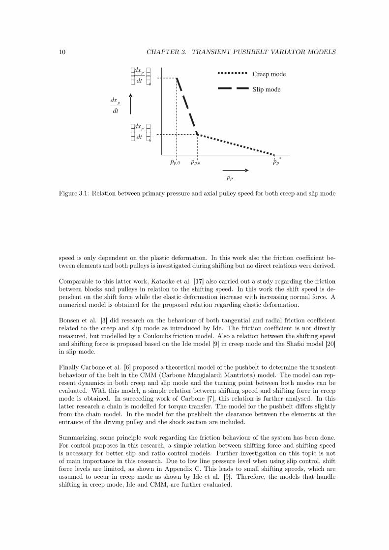
The research from Ide was expanded [9]. This work shows that the maximal shifting speed inthe pushbelt CVT is limited by the orifice of the primary valve, but not depended on the inputspeed. Therefore the equation given in the previous work [8] only holds for relative small shiftingspeeds. Two shifting modes can be defined, creep mode, with a maximal shifting speed dependenton input speed and slip mode where radial slip between the belt and pulleys occurs. In Figure3.1 a simple visualization of these two modes is represented. In slip mode less force is needed toachieve increasing shifting speeds, compared to creep mode.
Shafai et al. [20] introduced a simple belt model based on kinematics and the steady state ratioof both clamping pressures. It was shown that when the pressure ratio differs from the steadystate situation, acceleration in axial direction of the primary pulley sheave is possible. The secondorder equation of motion derived, contains a representing mass of the sheave and a representingfriction or damping coefficient.
Fujimura et al. [13] stated that during shifting radial slip occurs over the whole contact arcof the pulley where the running radius decreases. At the pulley where the running radius in-creases elastic deformation of the elements occurs, pushing each element outwards. Since the nextundeformed element enters the pulley at the increased running radius, the running radius of thetotal belt increases by each element that enters the pulley during the shifting cycles. Shifting
9
10 CHAPTER 3. TRANSIENT PUSHBELT VARIATOR MODELS
pp*
pp,hpp,0
0
dt
dx p
dt
dx p
pp
Creep mode
Slip mode
h
p
dt
dx
Figure 3.1: Relation between primary pressure and axial pulley speed for both creep and slip mode
speed is only dependent on the plastic deformation. In this work also the friction coefficient be-tween elements and both pulleys is investigated during shifting but no direct relations were derived.
Comparable to this latter work, Kataoke et al. [17] also carried out a study regarding the frictionbetween blocks and pulleys in relation to the shifting speed. In this work the shift speed is de-pendent on the shift force while the elastic deformation increase with increasing normal force. Anumerical model is obtained for the proposed relation regarding elastic deformation.
Bonsen et al. [3] did research on the behaviour of both tangential and radial friction coefficientrelated to the creep and slip mode as introduced by Ide. The friction coefficient is not directlymeasured, but modelled by a Coulombs friction model. Also a relation between the shifting speedand shifting force is proposed based on the Ide model [9] in creep mode and the Shafai model [20]in slip mode.
Finally Carbone et al. [6] proposed a theoretical model of the pushbelt to determine the transientbehaviour of the belt in the CMM (Carbone Mangialardi Mantriota) model. The model can rep-resent dynamics in both creep and slip mode and the turning point between both modes can beevaluated. With this model, a simple relation between shifting speed and shifting force in creepmode is obtained. In succeeding work of Carbone [7], this relation is further analysed. In thislatter research a chain is modelled for torque transfer. The model for the pushbelt differs slightlyfrom the chain model. In the model for the pushbelt the clearance between the elements at theentrance of the driving pulley and the shock section are included.
Summarizing, some principle work regarding the friction behaviour of the system has been done.For control purposes in this research, a simple relation between shifting force and shifting speedis necessary for better slip and ratio control models. Further investigation on this topic is notof main importance in this research. Due to low line pressure level when using slip control, shiftforce levels are limited, as shown in Appendix C. This leads to small shifting speeds, which areassumed to occur in creep mode as shown by Ide et al. [9]. Therefore, the models that handleshifting in creep mode, Ide and CMM, are further evaluated.
3.2. TRANSIENT MODELS 11
3.2 Transient modelsTransient variator models describe the relation between the CVT shift speed rg and clampingforces in the variator. The models to be compared are further explained in the next section.
3.2.1 Ide’s modelThe model of Ide is based on experimental results. During his study a number of ratio changeexperiments were carried out with various settings of pressures, primary speed, load and speedratio. The resulting model can be expressed as
rg = ki(rg)ωp [Fp − FsΨ(rg, τ)] (3.1)
where ki(rg) is an experimentally obtained constant, which depends on the geometric ratio rg. Ψrepresents the pulley thrust ratio necessary for steady state behaviour respectively, as defined inthe next section. Eq. (3.1) relates the shift speed to the shift force (Fp−FsΨ) and input speed ωp.Analysing ki(rg) gives a parameter, which can be divided in two parts, i.e. a ratio independentpart and a dependent part, transforming axial pulley speed to the rate of ratio change.
ki(rg) = ki,0rg
xp(3.2)
where xp denotes the axial speed of the primary pulley.
Eq. (3.1) holds in creep mode, while in slip mode the rate of change of the radial position ofthe belt on the pulley is independent of input speed. It is thought that the shifting speed alsodepends on the bending of the pulleys, proportional to the absolute shifting force. This shouldbe compensated in the constant ki(rg). In this model little physical explanation is given and Eq.(3.1) is estimated on experimental results. Also no difference between up- and downshifting isdistinguished.
3.2.2 CMM modelIn contrast to Ide’s model, the CMM model ([5], [7]) originates from a theoretical investigationpreformed on a one-dimensional model, while friction forces are modelled on the basis of Coulombfriction hypothesis. Also in this model a creep mode and slip mode can be distinguished. In thecreep mode, close to the steady state operation point, a linear dependency between shift speedand shift force can be estimated by
rg = ωp∆β(Fs)kc(rg)[ln
Fp
Fs− lnΨ(rg, τ)
](3.3)
where ∆β = max |β∗ − β| is the maximum amplitude of the wedge half-angle variations alongthe contact arc. The groove angle is, indeed, not constant along the wrapped arc because of thepulley bending due to elastic deformation and clearance in the bearings. β∗ is the non-uniformwedge half-angle of the deformed pulley, whereas β is the wedge half-angle of the undeformedpulley. the difference (β∗ − β) is described on the basis of the Sattler’s model [19], by means ofsimple trigonometric functions. The quantity ∆β depends on the clamping forces acting on thetwo pulleys always being of the order ∼ 10−3 [rad]. Eq. (3.3) shows that creep mode shifting takesplace only due to bending of the pulley sheaves. kc(rg) is a known function calculated using thetheoretical model, in contrast to ki(rg) from the Ide model. The derivation of this latter term isgiven in Appendix F
Besides the physical explanation of the shifting behaviour in creep mode, the CMM model hasanother big difference with the model of Ide. By taking the logarithm of the shifting force, adistinction between up- and downshifting can be made, based on dimensional analysis, explainedin Appendix E. This results in a symmetrical up- and downshifting around rg = 1, dependent onthe logarithmic of the shift force.
12 CHAPTER 3. TRANSIENT PUSHBELT VARIATOR MODELS
3.3 Pulley thrust ratioAll models for transient behaviour use the pulley thrust ratio Ψ, as defined by Vroemen [24].
Ψ(rg, τ) =F ∗
p
Fs(3.4)
where F ∗p denotes the primary clamping force needed to maintain stationary CVT speed ratio.
This pulley thrust ratio is dependent on the geometric ratio rg and torque ratio τ .
Measurements of Ψ are carried out at a test rig, where two electrical motors are both driving andbraking the CK2-CVT, as shown in Appendix C. During the experiments to obtain this thrustratio for different operating point, it became clear that it also was depending on the amount ofsecondary pressure ps. Due to limitations of the test rig this could not be measured for all workingpoint as shown in Appendix D. In this research on slip control, the results from measurements atminimum pressure levels are sufficient and the influence of increased secondary pressure will beneglected.
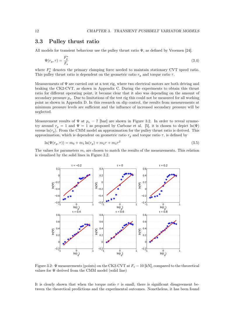
Measurement results of Ψ at ps = 7 [bar] are shown in Figure 3.2. In order to reveal symme-try around rg = 1 and Ψ = 1 as proposed by Carbone et al. [5], it is chosen to depict ln(Ψ)versus ln(rg). From the CMM model an approximation for the pulley thrust ratio is derived. Thisapproximation, which is dependent on geometric ratio rg and torque ratio τ , is defined by
ln(Ψ(rg, τ)) = m0 + m1 ln(rg) + m2τ + m3τ2 (3.5)
The values for parameters mi are chosen to match the results of the measurements. This relationis visualized by the solid lines in Figure 3.2.
−1 0 1−0.8
−0.6
−0.4
−0.2
0
0.2τ = −0.2
ln(rg)
ln(Ψ
)
−1 0 1−0.6
−0.4
−0.2
0
0.2
0.4τ = 0
ln(rg)
ln(Ψ
)
−1 0 1−0.4
−0.2
0
0.2
0.4
0.6τ = 0.2
ln(rg)
ln(Ψ
)
−1 0 1−0.2
0
0.2
0.4
0.6
0.8τ = 0.4
ln(rg)
ln(Ψ
)
−1 0 1−0.2
0
0.2
0.4
0.6
0.8τ = 0.6
ln(rg)
ln(Ψ
)
−1 0 1−0.2
0
0.2
0.4
0.6
0.8τ = 0.8
ln(rg)
ln(Ψ
)
Figure 3.2: Ψ measurements (points) on the CK2-CVT at Fs = 10 [kN], compared to the theoreticalvalues for Ψ derived from the CMM model (solid line)
It is clearly shown that when the torque ratio τ is small, there is significant disagreement be-tween the theoretical predictions and the experimental outcomes. Nonetheless, it has been found
3.4. VALIDATION AND COMPARISON OF TRANSIENT MODELS 13
that in the case of used belts a very good agreement occurs also at low torque levels [5]. This maysupport the idea that band-elements interaction, not considered by the CMM model, may have akey role at small torque ratios. Thus, further investigation should be carried out. However, sincethe slip control strategy needs relatively high torque ratio values, this allows the use of the CMMmodel in the subsequent sections.
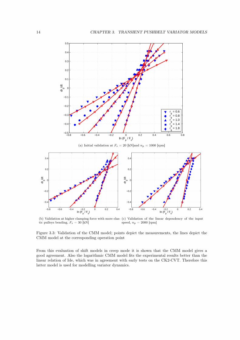
3.4 Validation and comparison of transient modelsIn the previous sections two models were introduced. The Ide model, based on experimental re-sults and the CMM model based on theoretical calculations. The latter model is investigated andvalidated by spin-loss measurements at a variator preformed by Carbone et al. [5]. This variatoris preferred since, at the Jatco CK2-CVT side effects of the other parts of the transmission shouldbe taken into account.
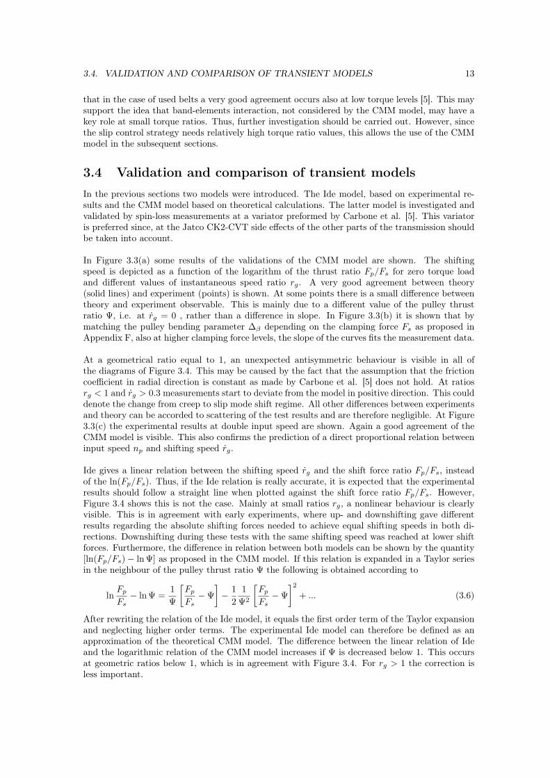
In Figure 3.3(a) some results of the validations of the CMM model are shown. The shiftingspeed is depicted as a function of the logarithm of the thrust ratio Fp/Fs for zero torque loadand different values of instantaneous speed ratio rg. A very good agreement between theory(solid lines) and experiment (points) is shown. At some points there is a small difference betweentheory and experiment observable. This is mainly due to a different value of the pulley thrustratio Ψ, i.e. at rg = 0 , rather than a difference in slope. In Figure 3.3(b) it is shown that bymatching the pulley bending parameter ∆β depending on the clamping force Fs as proposed inAppendix F, also at higher clamping force levels, the slope of the curves fits the measurement data.
At a geometrical ratio equal to 1, an unexpected antisymmetric behaviour is visible in all ofthe diagrams of Figure 3.4. This may be caused by the fact that the assumption that the frictioncoefficient in radial direction is constant as made by Carbone et al. [5] does not hold. At ratiosrg < 1 and rg > 0.3 measurements start to deviate from the model in positive direction. This coulddenote the change from creep to slip mode shift regime. All other differences between experimentsand theory can be accorded to scattering of the test results and are therefore negligible. At Figure3.3(c) the experimental results at double input speed are shown. Again a good agreement of theCMM model is visible. This also confirms the prediction of a direct proportional relation betweeninput speed np and shifting speed rg.
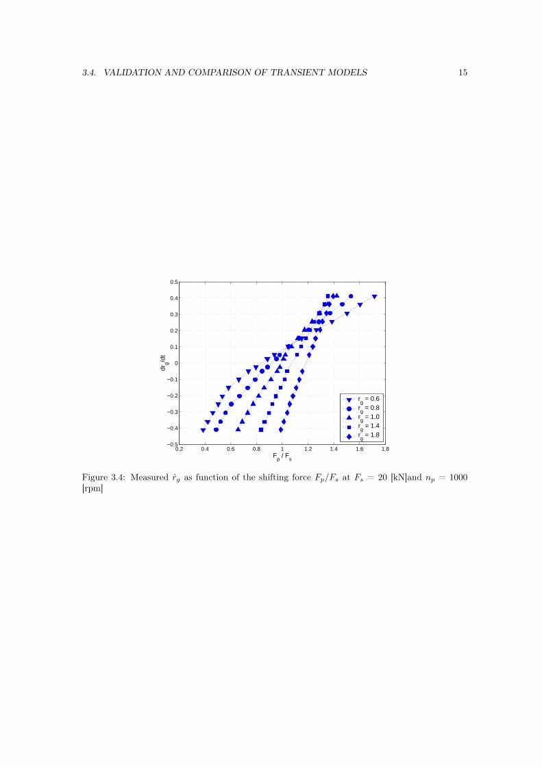
Ide gives a linear relation between the shifting speed rg and the shift force ratio Fp/Fs, insteadof the ln(Fp/Fs). Thus, if the Ide relation is really accurate, it is expected that the experimentalresults should follow a straight line when plotted against the shift force ratio Fp/Fs. However,Figure 3.4 shows this is not the case. Mainly at small ratios rg, a nonlinear behaviour is clearlyvisible. This is in agreement with early experiments, where up- and downshifting gave differentresults regarding the absolute shifting forces needed to achieve equal shifting speeds in both di-rections. Downshifting during these tests with the same shifting speed was reached at lower shiftforces. Furthermore, the difference in relation between both models can be shown by the quantity[ln(Fp/Fs)− lnΨ] as proposed in the CMM model. If this relation is expanded in a Taylor seriesin the neighbour of the pulley thrust ratio Ψ the following is obtained according to
lnFp
Fs− lnΨ =
1Ψ
[Fp
Fs−Ψ
]− 1
21
Ψ2
[Fp
Fs−Ψ
]2+ ... (3.6)
After rewriting the relation of the Ide model, it equals the first order term of the Taylor expansionand neglecting higher order terms. The experimental Ide model can therefore be defined as anapproximation of the theoretical CMM model. The difference between the linear relation of Ideand the logarithmic relation of the CMM model increases if Ψ is decreased below 1. This occursat geometric ratios below 1, which is in agreement with Figure 3.4. For rg > 1 the correction isless important.
14 CHAPTER 3. TRANSIENT PUSHBELT VARIATOR MODELS
−0.8 −0.6 −0.4 −0.2 0 0.2 0.4 0.6 0.8−0.5
−0.4
−0.3
−0.2
−0.1
0
0.1
0.2
0.3
0.4
0.5
ln (Fp / F
s)
drg/d
t
rg = 0.6
rg = 0.8
rg = 1.0
rg = 1.4
rg = 1.8
(a) Initial validation at Fs = 20 [kN]and np = 1000 [rpm]
−0.8 −0.6 −0.4 −0.2 0 0.2 0.4
−0.4
−0.2
0
0.2
0.4
ln (Fp / F
s)
drg/d
t
(b) Validation at higher clamping force with more elas-tic pulleys bending, Fs = 30 [kN[
−0.8 −0.6 −0.4 −0.2 0 0.2 0.4
−0.4
−0.2
0
0.2
0.4
ln (Fp / F
s)
drg/d
t
(c) Validation of the linear dependency of the inputspeed, np = 2000 [rpm]
Figure 3.3: Validation of the CMM model; points depict the measurements, the lines depict theCMM model at the corresponding operation point
From this evaluation of shift models in creep mode it is shown that the CMM model gives agood agreement. Also the logarithmic CMM model fits the experimental results better than thelinear relation of Ide, which was in agreement with early tests on the CK2-CVT. Therefore thislatter model is used for modelling variator dynamics.
3.4. VALIDATION AND COMPARISON OF TRANSIENT MODELS 15
0.2 0.4 0.6 0.8 1 1.2 1.4 1.6 1.8−0.5
−0.4
−0.3
−0.2
−0.1
0
0.1
0.2
0.3
0.4
0.5
Fp / F
s
drg/d
t
rg = 0.6
rg = 0.8
rg = 1.0
rg = 1.4
rg = 1.8
Figure 3.4: Measured rg as function of the shifting force Fp/Fs at Fs = 20 [kN]and np = 1000[rpm]

16 CHAPTER 3. TRANSIENT PUSHBELT VARIATOR MODELS
Chapter 4
Modeling system dynamics
In contrast to the model in the previous work from Bonsen et al. [1], both geometric ratio rg
and relative belt slip ν are taken into account here. Therefore, slip dynamics will differ from theprevious models as will be shown in the next section. Subsequent, the variator and actuationdynamics are derived and interaction of the complete plant is analysed.
4.1 Variator dynamics
In contrast to the previous work, the geometric ratio is not regarded as quasi-stationary. Fromanalysis in Chapter 2 it became clear that the assumption of geometric dynamics being muchslower than slip dynamics does not hold for fast shifting events. Therefore derivation of Eq. (2.2)gives
ν =rsrg − rg rs
r2g
(4.1)
where rg is given by the CMM model (Eq. (3.3)) and the derivative of the speed ratio rs is givenby
rs =ωpωs − ωsωp
ω2p
(4.2)
J e
J s
r g
w p
w s
T e
T d
C V TT p
T s
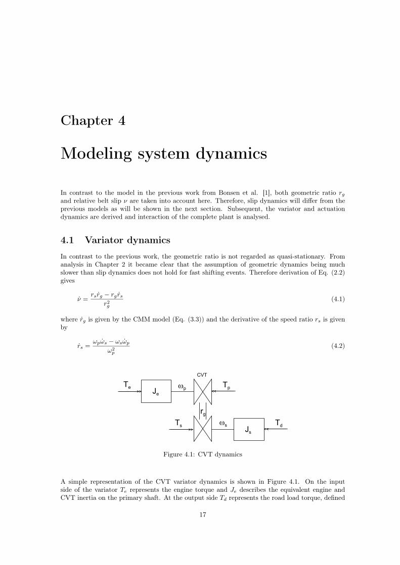
Figure 4.1: CVT dynamics
A simple representation of the CVT variator dynamics is shown in Figure 4.1. On the inputside of the variator Te represents the engine torque and Je describes the equivalent engine andCVT inertia on the primary shaft. At the output side Td represents the road load torque, defined
17
18 CHAPTER 4. MODELING SYSTEM DYNAMICS
by road load conditions, and Js describes the equivalent vehicle inertia on the secondary shaft.The dynamics of the primary and secondary shaft of the CVT variator are given by
ωp =Te − Tp
Je(4.3)
ωs =Ts − Td
Js(4.4)
with Tp and Ts denoting the torque on the primary and secondary shaft respectively. These torquesgenerated on both shafts of the variator are described, based on Eq. (2.1), by
Tp,s =2Fsµeff (ν, rg)Rp,s
cos β(4.5)
In this description torque losses are neglected. It is assumed that these losses are not significantfor the modelling of variator dynamics.
Substituting Eqs. (3.3), (4.2), (4.3), (4.4) and (4.5) in Eq. (4.1) leads to
ν =1ωp
(−2FsRsµeff (ν, rg)
Jsrg cos β+
Td
Jsrg
)+
1− ν
ωp
(−2FsRsrgµeff (ν, rg)
Je cos β+
Te
Je
)+
1− ν
rgrg (4.6)
Compared to the model with neglecting geometric ratio dynamics described by Bonsen et al. [2],the last term in Eq. (4.6) is added, since ratio changing dynamics are not negligible, i.e. rg 6= 0 .
The amount of friction between pulley and belt is related to the slip in the variator. The frictioncoefficient used in this model is therefore described by
µeff (ν, rg) = k1i(rg)ν + k2i(rg) (4.7)
which is a piecewise linear approximation of the results shown in Figure 1. The ratio dependencyis taken into account by the choice of k1i and k2i. The micro slip regime is denoted by i = 1,whereas i = 2 denotes the macro slip regime.
Besides the amount of slip ν, also the ratio rg is a control variable in the controller proposedin Chapter 5. Since the primary axial pulley position xp is measured and to avoid the nonlinearcalculation from xp to rg, this linear position is used as control variable. Considering this, thedynamic equations are rewritten to
ν =1ωp
(−Fsxpµeff (ν, rg)
sinβJsr2g
+Td
Jsrg
)+
1− ν
ωp
(−Fsxpµeff (ν, rg)
sinβJe+
Te
Je
)+(1−ν)
xp
xp[1+rgh(rg)]
(4.8)
and
xp = ωp∆βkc,x(rg)x2p
[ln
Fp
Fs− lnΨ(rg, τ)
](4.9)
where both h(rg) and kc,x(rg) are defined in Appendix F. Defining the state vector x =[
ν xp
]T ,input vector u =
[Fs ∆ln F Te Td
]T and output vector y = x, the dynamics can be de-scribed, when linearized around a certain working point x =
[ν0 xp0
]T , by
x = Avarx + Bvaru (4.10)y = Cvarx (4.11)
Note that the terms dependent on ratio are also related to the axial primary pulley position. InAppendix G a more complete derivation of the linearized model is given. It is assumed that ν0
4.2. ACTUATION SYSTEM DYNAMICS 19
100 [%] and d1 1 and higher order terms of ν can be neglected. This results in
Avar =[
a11 a12
a21 a22
]and Bvar =
[b11 b12 b13 b14
b21 b22 0 0
]with
a11 = 1ωp0
(Fs0xp0sin β
((k2i−k1i)
Je− k1i
r2g0Js
)− Te0
Je
)+ ωp∆βkc,xxp0[1 + rg0h)]
(∂∆ln F
∂ν −∆ln F0
)a12 = 1
ωp0
(−Td0(1+rg0h)
xp0Jsrg0+ Fs0k2i
sin β
(2[1+rg0h]−1
Jsr2g0
− 1Je
))+ωp∆βkc,xxp0[1 + rg0h)]
(∆ln F0
c∂c
∂xp+ ∆ln F0
rg0+ ∂∆ln F
∂xp
)a21 = ωp∆βkc,xx2
p0∂∆ln F
∂ν
a22 = ωp∆βx2p0
(2kc,x∆ln F0
xp0+ ∆ln F0
∂kc,x
∂xp+ kc,x
∂∆ln F
∂xp
)and
b11 = − xp0k2i
ωp0 sin β
(1Je
+ 1r2
g0Js
)− ωp∆βkc,xxp0[1 + rg0h] 1
Fs0
b12 = ωp∆βkc,xxp0[1 + rg0h]b13 = 1
Jeωp0
b14 = 1Jsωp0rg0
b21 = −ωp∆βkc,x1
Fs0
b22 = ωp∆βkc,x
The partial derivatives can be found in Appendix G.
In case of the CMM model, the input ∆ln F0 represents the logarithm of the shift force ratioFp/Fs minus the logarithm of the pulley thrust ratio Ψ.
∆ln F0 = lnFp0
Fs0− lnΨ0 (4.12)
Furthermore, the terms Te0 and Td0 are calculated to match the maximum torque that can betransmitted in the chosen working point, leading to
Te0 =xp0Fs0µeff0
sinβ(4.13)
Td0 =Te0
rg0(4.14)
This results in the transfer function Hvar for the variator dynamics.
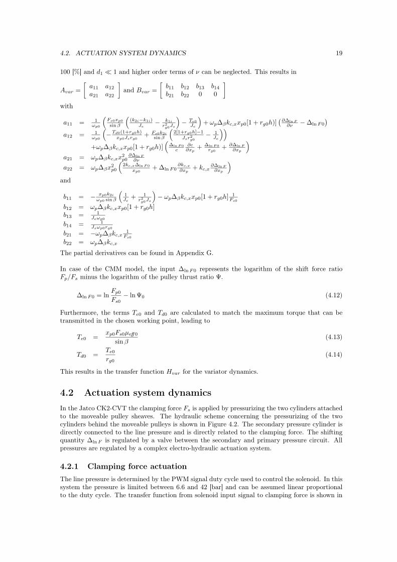
4.2 Actuation system dynamicsIn the Jatco CK2-CVT the clamping force Fs is applied by pressurizing the two cylinders attachedto the moveable pulley sheaves. The hydraulic scheme concerning the pressurizing of the twocylinders behind the moveable pulleys is shown in Figure 4.2. The secondary pressure cylinder isdirectly connected to the line pressure and is directly related to the clamping force. The shiftingquantity ∆ln F is regulated by a valve between the secondary and primary pressure circuit. Allpressures are regulated by a complex electro-hydraulic actuation system.
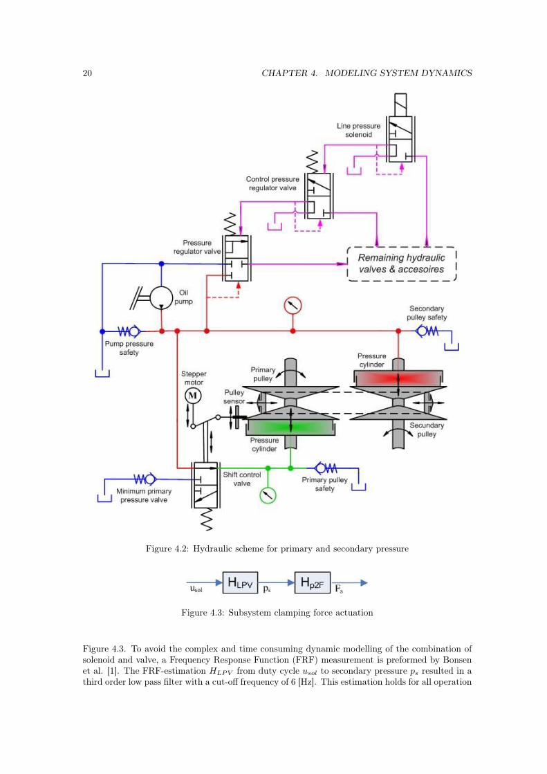
4.2.1 Clamping force actuationThe line pressure is determined by the PWM signal duty cycle used to control the solenoid. In thissystem the pressure is limited between 6.6 and 42 [bar] and can be assumed linear proportionalto the duty cycle. The transfer function from solenoid input signal to clamping force is shown in
20 CHAPTER 4. MODELING SYSTEM DYNAMICS
Figure 4.2: Hydraulic scheme for primary and secondary pressure
Figure 4.3: Subsystem clamping force actuation
Figure 4.3. To avoid the complex and time consuming dynamic modelling of the combination ofsolenoid and valve, a Frequency Response Function (FRF) measurement is preformed by Bonsenet al. [1]. The FRF-estimation HLPV from duty cycle usol to secondary pressure ps resulted in athird order low pass filter with a cut-off frequency of 6 [Hz]. This estimation holds for all operation
4.2. ACTUATION SYSTEM DYNAMICS 21
points. To rewrite the pressure to an actual clamping force, both the centrifugal force and springpre-load force should be added, resulting in
Fs = Asps + fcsω2s + kspr[xs,max − xs] + Fspr,0 (4.15)
Here As and fcs represent the pressure cylinder area and centrifugal coefficient of the secondarypulley respectively. kspr is the spring constant of the spring, preloading the moveable secondarypulley sheave and Fspr,0 the preload by the spring at its initial position. xs represents the axialposition of this sheave.
The linearized transfer function HLP from duty cycle usol to secondary clamping force Fs isobtained by
HLP =Fs
usol= HLPV Hp2F (4.16)
where Hp2F is equal to the secondary cylinder surface As. Since variables ωs and xs are lost dueto linearizing of Eq. (4.15), transfer function Hp2F is dependent on the chosen working point, i.e.speed and CVT ratio dependent.
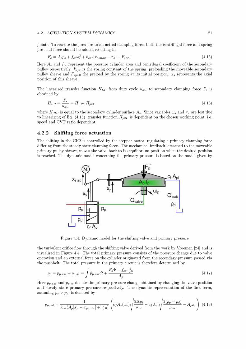
4.2.2 Shifting force actuationThe shifting in the CK2 is controlled by the stepper motor, regulating a primary clamping forcediffering from the steady state clamping force. The mechanical feedback, attached to the moveableprimary pulley sheave, moves the valve back to its equilibrium position when the desired positionis reached. The dynamic model concerning the primary pressure is based on the model given by
Figure 4.4: Dynamic model for the shifting valve and primary pressure
the turbulent orifice flow through the shifting valve derived from the work by Vroemen [24] and isvisualized in Figure 4.4. The total primary pressure consists of the pressure change due to valveoperation and an external force on the cylinder originated from the secondary pressure passed viathe pushbelt. The total pressure in the primary circuit is therefore determined by
pp = pp,val + pp,ss =∫
pp,valdt +FsΨ− fcpω
2p0
Ap(4.17)
Here pp,val and pp,ss denote the primary pressure change obtained by changing the valve positionand steady state primary pressure respectively. The dynamic representation of the first term,assuming ps > pp, is denoted by
pp,val =1
koil(Ap[xp − xp,min] + Vp0)
(cfAv(xv)
√2∆pi
ρoil− cfApl
√2(pp − pd)
ρoil−Apxp
)(4.18)
22 CHAPTER 4. MODELING SYSTEM DYNAMICS
Here koil and ρoil are the compressibility and density properties of the ATF-oil respectively; Ap
the primary cylinder surface, Vp0 the initial primary cylinder volume, Apl the primary leakageorifice and cf represents the orifice resistance coefficient. Furthermore, ∆pi is the pressure dropover the valve, depending on the position of the valve xv. Also the orifice surface Av depends onthis position. The shifting valve position is dependent on stepper motor and axial pulley positionand it is assumed that xv = 0 when the valve is closing both hydraulic circuits. Finally, the axialpulley speed is determined by the CMM model as given in Eq. (4.9). This results in
∆pi(xv > 0) = ps − pp (4.19)∆pi(xv > 0) = pp − pd (4.20)
xv =xstep − [xp − xp,min]
2(4.21)
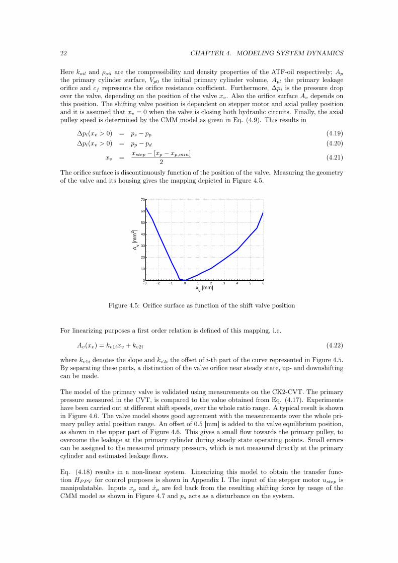
The orifice surface is discontinuously function of the position of the valve. Measuring the geometryof the valve and its housing gives the mapping depicted in Figure 4.5.
−3 −2 −1 0 1 2 3 4 5 60
10
20
30
40
50
60
70
xv [mm]
Av [m
m2 ]
Figure 4.5: Orifice surface as function of the shift valve position
For linearizing purposes a first order relation is defined of this mapping, i.e.
Av(xv) = kv1ixv + kv2i (4.22)
where kv1i denotes the slope and kv2i the offset of i-th part of the curve represented in Figure 4.5.By separating these parts, a distinction of the valve orifice near steady state, up- and downshiftingcan be made.
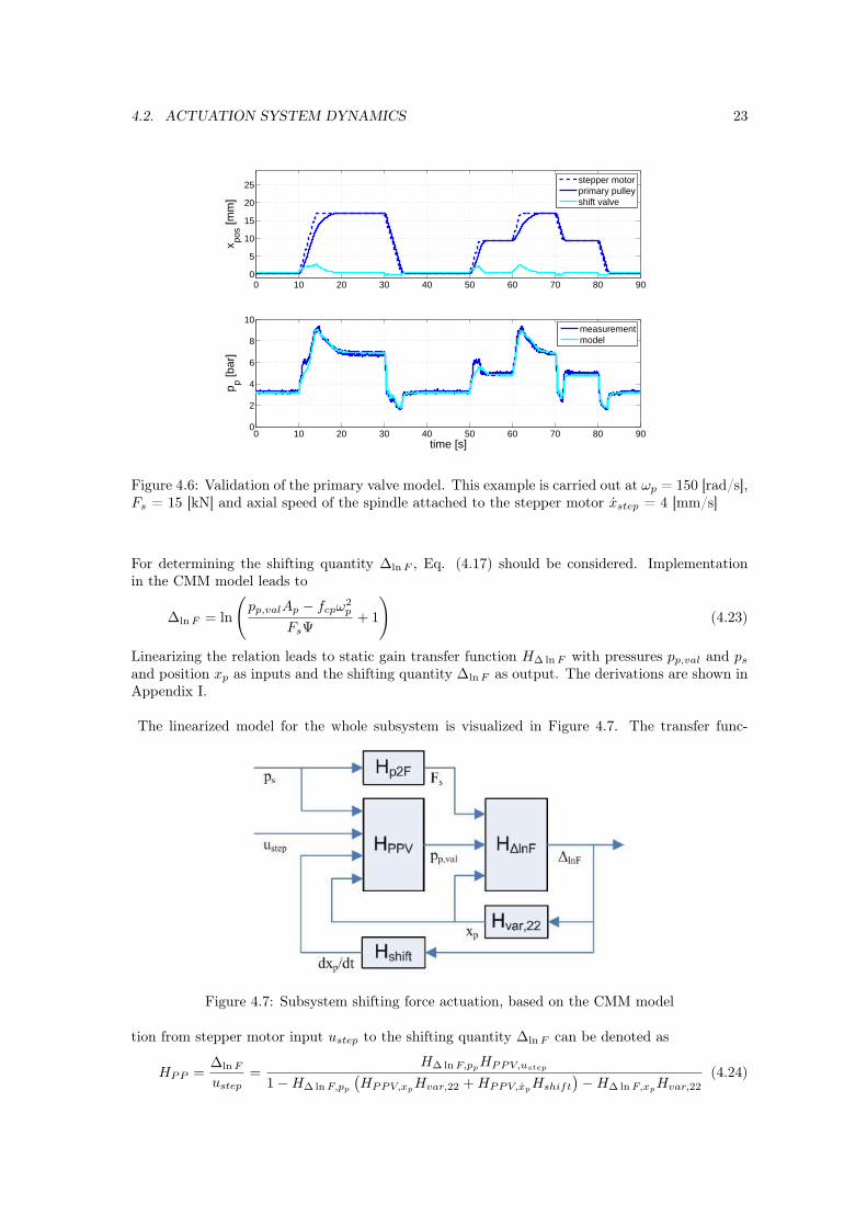
The model of the primary valve is validated using measurements on the CK2-CVT. The primarypressure measured in the CVT, is compared to the value obtained from Eq. (4.17). Experimentshave been carried out at different shift speeds, over the whole ratio range. A typical result is shownin Figure 4.6. The valve model shows good agreement with the measurements over the whole pri-mary pulley axial position range. An offset of 0.5 [mm] is added to the valve equilibrium position,as shown in the upper part of Figure 4.6. This gives a small flow towards the primary pulley, toovercome the leakage at the primary cylinder during steady state operating points. Small errorscan be assigned to the measured primary pressure, which is not measured directly at the primarycylinder and estimated leakage flows.
Eq. (4.18) results in a non-linear system. Linearizing this model to obtain the transfer func-tion HPPV for control purposes is shown in Appendix I. The input of the stepper motor ustep ismanipulatable. Inputs xp and xp are fed back from the resulting shifting force by usage of theCMM model as shown in Figure 4.7 and ps acts as a disturbance on the system.
4.2. ACTUATION SYSTEM DYNAMICS 23
0 10 20 30 40 50 60 70 80 900
5
10
15
20
25
x pos [m
m]
stepper motorprimary pulleyshift valve
0 10 20 30 40 50 60 70 80 900
2
4
6
8
10
time [s]
p p [bar
]
measurementmodel
Figure 4.6: Validation of the primary valve model. This example is carried out at ωp = 150 [rad/s],Fs = 15 [kN] and axial speed of the spindle attached to the stepper motor xstep = 4 [mm/s]
For determining the shifting quantity ∆ln F , Eq. (4.17) should be considered. Implementationin the CMM model leads to
∆ln F = ln
(pp,valAp − fcpω
2p
FsΨ+ 1
)(4.23)
Linearizing the relation leads to static gain transfer function H∆ ln F with pressures pp,val and ps
and position xp as inputs and the shifting quantity ∆ln F as output. The derivations are shown inAppendix I.
The linearized model for the whole subsystem is visualized in Figure 4.7. The transfer func-
Figure 4.7: Subsystem shifting force actuation, based on the CMM model
tion from stepper motor input ustep to the shifting quantity ∆ln F can be denoted as
HPP =∆ln F
ustep=
H∆ ln F,ppHPPV,ustep
1−H∆ ln F,pp
(HPPV,xp
Hvar,22 + HPPV,xpHshift
)−H∆ ln F,xp
Hvar,22
(4.24)
24 CHAPTER 4. MODELING SYSTEM DYNAMICS
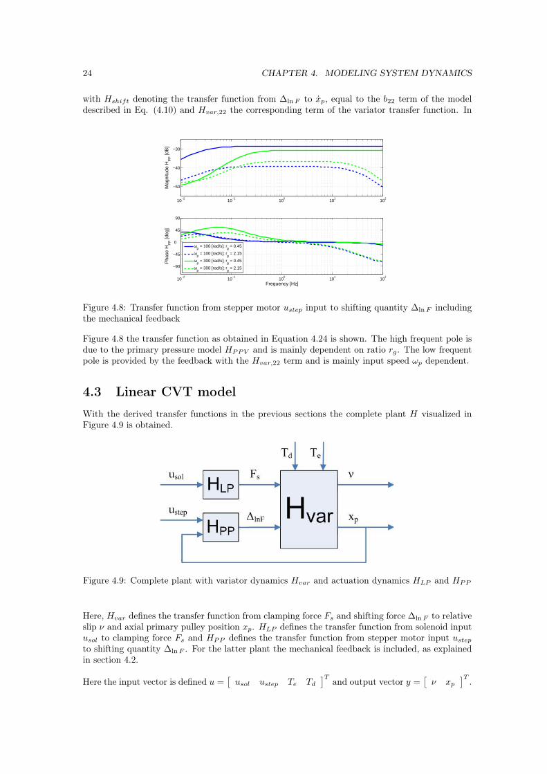
with Hshift denoting the transfer function from ∆ln F to xp, equal to the b22 term of the modeldescribed in Eq. (4.10) and Hvar,22 the corresponding term of the variator transfer function. In
10−2
10−1
100
101
102
−50
−40
−30
Mag
nitu
de H
PP [d
B]
10−2
10−1
100
101
102
−90
−45
0
45
90
Pha
se H
PP [d
eg]
Frequency [Hz]
ωp = 100 [rad/s]; r
g = 0.45
ωp = 100 [rad/s]; r
g = 2.15
ωp = 300 [rad/s]; r
g = 0.45
ωp = 300 [rad/s]; r
g = 2.15
Figure 4.8: Transfer function from stepper motor ustep input to shifting quantity ∆ln F includingthe mechanical feedback
Figure 4.8 the transfer function as obtained in Equation 4.24 is shown. The high frequent pole isdue to the primary pressure model HPPV and is mainly dependent on ratio rg. The low frequentpole is provided by the feedback with the Hvar,22 term and is mainly input speed ωp dependent.
4.3 Linear CVT model
With the derived transfer functions in the previous sections the complete plant H visualized inFigure 4.9 is obtained.
Figure 4.9: Complete plant with variator dynamics Hvar and actuation dynamics HLP and HPP
Here, Hvar defines the transfer function from clamping force Fs and shifting force ∆ln F to relativeslip ν and axial primary pulley position xp. HLP defines the transfer function from solenoid inputusol to clamping force Fs and HPP defines the transfer function from stepper motor input ustep
to shifting quantity ∆ln F . For the latter plant the mechanical feedback is included, as explainedin section 4.2.
Here the input vector is defined u =[
usol ustep Te Td
]T and output vector y =[
ν xp
]T .
4.4. INTERACTION ANALYSIS 25
The derived linearized system will be used for controller design. The model has 4 inputs, whereonly usol and ustep can be manipulated. In the present setup of the hydraulic system, the solenoidinput usol controls the slip and the input of the stepper motor ustep controls the geometric ratiothat is related to the primary axial pulley position. The input torque Te is controlled by the drivervia the throttle pedal, where output torque Td is determined by the road conditions. The lattertwo can therefore be regarded as disturbances on the system.
10−2
10−1
100
101
102
−150
−100
−50
0
50
Mag
nitu
de H
11 [d
B]
10−2
10−1
100
101
102
−200
−100
0
100
200
Pha
se H
11 [d
eg]
10−2
10−1
100
101
102
−150
−100
−50
0
Mag
nitu
de H
12 [d
B]
10−2
10−1
100
101
102
−200
−100
0
100
Pha
se H
12 [d
eg]
10−2
10−1
100
101
102
−200
−150
−100
−50
0
Mag
nitu
de H
21 [d
B]
10−2
10−1
100
101
102
−200
−100
0
100
200
Frequency [Hz]
Pha
se H
21 [d
eg]
10−2
10−1
100
101
102
−200
−150
−100
−50
Mag
nitu
de H
22 [d
B]
10−2
10−1
100
101
102
−200
−150
−100
−50
0
Frequency [Hz]
Pha
se H
22 [d
eg]
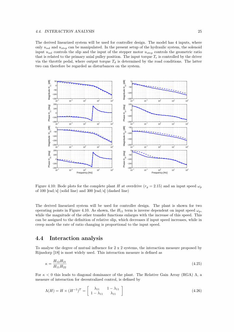
Figure 4.10: Bode plots for the complete plant H at overdrive (rg = 2.15) and an input speed ωp
of 100 [rad/s] (solid line) and 300 [rad/s] (dashed line)
The derived linearized system will be used for controller design. The plant is shown for twooperating points in Figure 4.10. As shown, the H11 term is inverse dependent on input speed ωp,while the magnitude of the other transfer functions enlarges with the increase of this speed. Thiscan be assigned to the definition of relative slip, which decreases if input speed increases, while increep mode the rate of ratio changing is proportional to the input speed.
4.4 Interaction analysis
To analyse the degree of mutual influence for 2 x 2 systems, the interaction measure proposed byRijnsdorp [18] is most widely used. This interaction measure is defined as
κ =H12H21
H11H22(4.25)
For κ < 0 this leads to diagonal dominance of the plant. The Relative Gain Array (RGA) Λ, ameasure of interaction for decentralized control, is defined by
Λ(H) = H × (H−1)T =[
λ11 1− λ11
1− λ11 λ11
](4.26)
26 CHAPTER 4. MODELING SYSTEM DYNAMICS
where × denotes element-by-element multiplication and
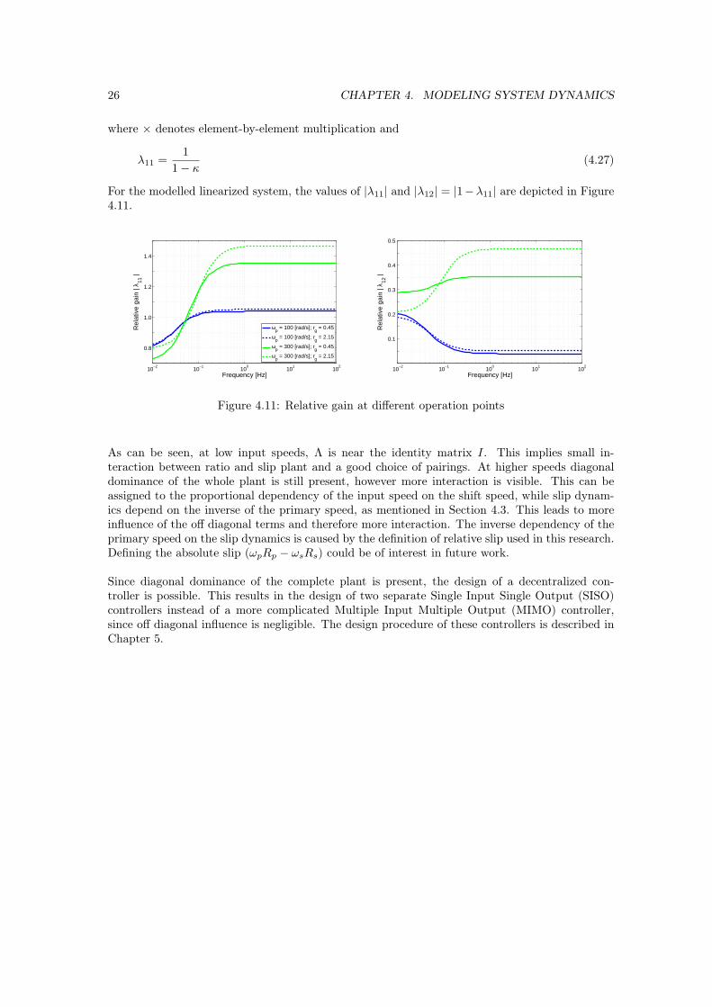
λ11 =1
1− κ(4.27)
For the modelled linearized system, the values of |λ11| and |λ12| = |1−λ11| are depicted in Figure4.11.
10−2
10−1
100
101
102
0.8
1.0
1.2
1.4
Frequency [Hz]
Rel
ativ
e ga
in |
λ 11 |
ωp = 100 [rad/s]; r
g = 0.45
ωp = 100 [rad/s]; r
g = 2.15
ωp = 300 [rad/s]; r
g = 0.45
ωp = 300 [rad/s]; r
g = 2.15
10−2
10−1
100
101
102
0.1
0.2
0.3
0.4
0.5
Frequency [Hz]R
elat
ive
gain
| λ 12
|
Figure 4.11: Relative gain at different operation points
As can be seen, at low input speeds, Λ is near the identity matrix I. This implies small in-teraction between ratio and slip plant and a good choice of pairings. At higher speeds diagonaldominance of the whole plant is still present, however more interaction is visible. This can beassigned to the proportional dependency of the input speed on the shift speed, while slip dynam-ics depend on the inverse of the primary speed, as mentioned in Section 4.3. This leads to moreinfluence of the off diagonal terms and therefore more interaction. The inverse dependency of theprimary speed on the slip dynamics is caused by the definition of relative slip used in this research.Defining the absolute slip (ωpRp − ωsRs) could be of interest in future work.
Since diagonal dominance of the complete plant is present, the design of a decentralized con-troller is possible. This results in the design of two separate Single Input Single Output (SISO)controllers instead of a more complicated Multiple Input Multiple Output (MIMO) controller,since off diagonal influence is negligible. The design procedure of these controllers is described inChapter 5.
Chapter 5
Control design and strategy
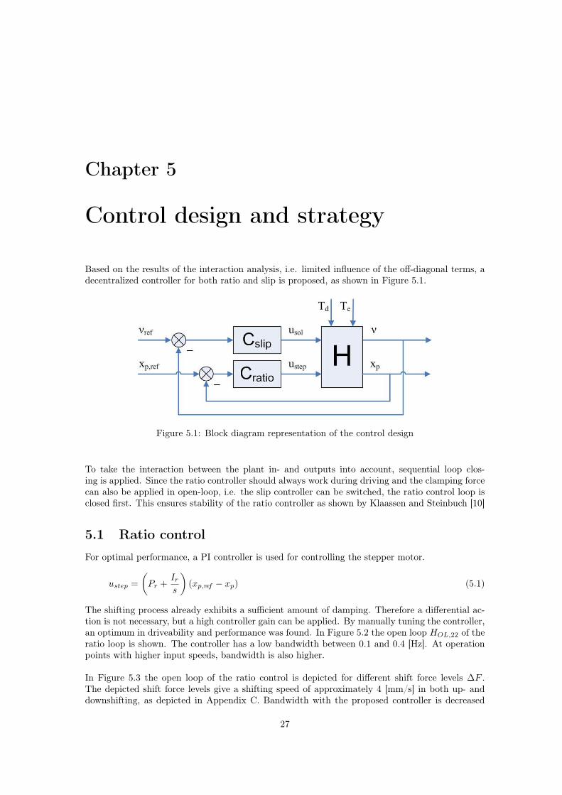
Based on the results of the interaction analysis, i.e. limited influence of the off-diagonal terms, adecentralized controller for both ratio and slip is proposed, as shown in Figure 5.1.
Figure 5.1: Block diagram representation of the control design
To take the interaction between the plant in- and outputs into account, sequential loop clos-ing is applied. Since the ratio controller should always work during driving and the clamping forcecan also be applied in open-loop, i.e. the slip controller can be switched, the ratio control loop isclosed first. This ensures stability of the ratio controller as shown by Klaassen and Steinbuch [10]
5.1 Ratio control
For optimal performance, a PI controller is used for controlling the stepper motor.
ustep =(
Pr +Ir
s
)(xp,ref − xp) (5.1)
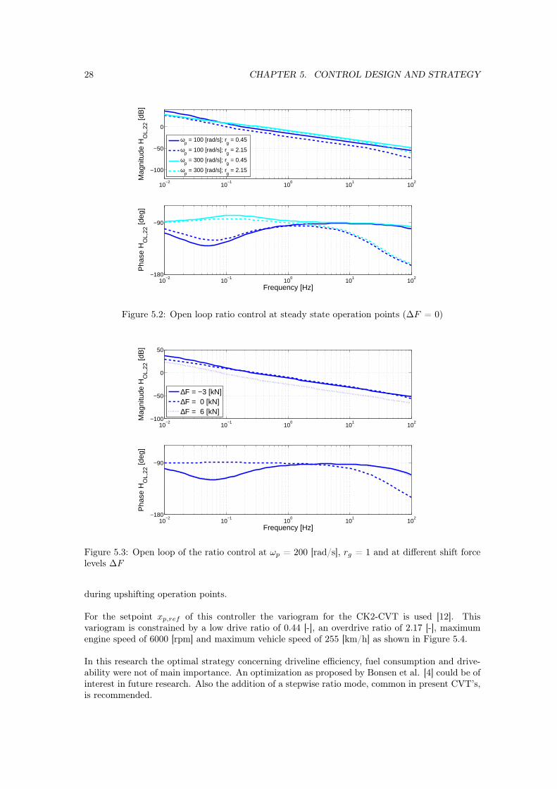
The shifting process already exhibits a sufficient amount of damping. Therefore a differential ac-tion is not necessary, but a high controller gain can be applied. By manually tuning the controller,an optimum in driveability and performance was found. In Figure 5.2 the open loop HOL,22 of theratio loop is shown. The controller has a low bandwidth between 0.1 and 0.4 [Hz]. At operationpoints with higher input speeds, bandwidth is also higher.
In Figure 5.3 the open loop of the ratio control is depicted for different shift force levels ∆F .The depicted shift force levels give a shifting speed of approximately 4 [mm/s] in both up- anddownshifting, as depicted in Appendix C. Bandwidth with the proposed controller is decreased
27
28 CHAPTER 5. CONTROL DESIGN AND STRATEGY
10−2
10−1
100
101
102
−100
−50
0
Mag
nitu
de H
OL,
22 [d
B]
10−2
10−1
100
101
102
−180
−90
Pha
se H
OL,
22 [d
eg]
Frequency [Hz]
ωp = 100 [rad/s]; r
g = 0.45
ωp = 100 [rad/s]; r
g = 2.15
ωp = 300 [rad/s]; r
g = 0.45
ωp = 300 [rad/s]; r
g = 2.15
Figure 5.2: Open loop ratio control at steady state operation points (∆F = 0)
10−2
10−1
100
101
102
−100
−50
0
50
Mag
nitu
de H
OL,
22 [d
B]
10−2
10−1
100
101
102
−180
−90
Pha
se H
OL,
22 [d
eg]
Frequency [Hz]
∆F = −3 [kN]∆F = 0 [kN]∆F = 6 [kN]
Figure 5.3: Open loop of the ratio control at ωp = 200 [rad/s], rg = 1 and at different shift forcelevels ∆F
during upshifting operation points.
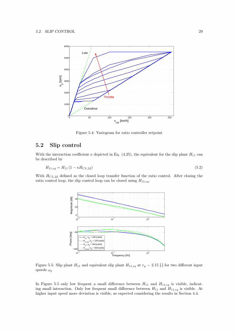
For the setpoint xp,ref of this controller the variogram for the CK2-CVT is used [12]. Thisvariogram is constrained by a low drive ratio of 0.44 [-], an overdrive ratio of 2.17 [-], maximumengine speed of 6000 [rpm] and maximum vehicle speed of 255 [km/h] as shown in Figure 5.4.
In this research the optimal strategy concerning driveline efficiency, fuel consumption and drive-ability were not of main importance. An optimization as proposed by Bonsen et al. [4] could be ofinterest in future research. Also the addition of a stepwise ratio mode, common in present CVT’s,is recommended.
5.2. SLIP CONTROL 29
0 50 100 150 200 2500
1000
2000
3000
4000
5000
6000
vcar
[km/h]
n p [rpm
]
Overdrive
Low
Throttle
Figure 5.4: Variogram for ratio controller setpoint
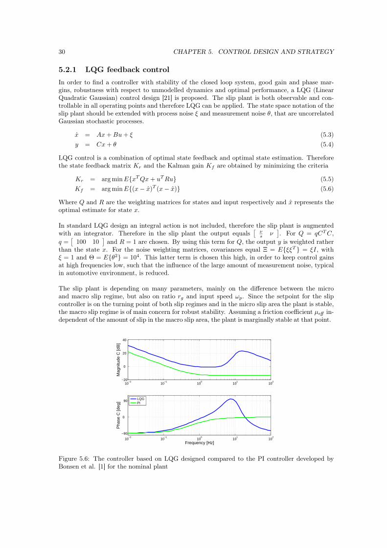
5.2 Slip controlWith the interaction coefficient κ depicted in Eq. (4.25), the equivalent for the slip plant H11 canbe described by
H11,eq = H11 (1− κHCL,22) (5.2)
With HCL,22 defined as the closed loop transfer function of the ratio control. After closing theratio control loop, the slip control loop can be closed using H11,eq.
10−2
10−1
100
0
20
40
Mag
nitu
de [d
B]
10−2
10−1
100
−180
−90
Pha
se [d
eg]
Frequency [Hz]
H11
; ωp = 100 [rad/s]
H11,eq
; ωp = 100 [rad/s]
H11
; ωp = 300 [rad/s]
H11,eq
; ωp = 300 [rad/s]
Figure 5.5: Slip plant H11 and equivalent slip plant H11,eq at rg = 2.15 [-] for two different inputspeeds ωp
In Figure 5.5 only low frequent a small difference between H11 and H11,eq is visible, indicat-ing small interaction. Only low frequent small difference between H11 and H11,eq is visible. Athigher input speed more deviation is visible, as expected considering the results in Section 4.4.
30 CHAPTER 5. CONTROL DESIGN AND STRATEGY
5.2.1 LQG feedback control
In order to find a controller with stability of the closed loop system, good gain and phase mar-gins, robustness with respect to unmodelled dynamics and optimal performance, a LQG (LinearQuadratic Gaussian) control design [21] is proposed. The slip plant is both observable and con-trollable in all operating points and therefore LQG can be applied. The state space notation of theslip plant should be extended with process noise ξ and measurement noise θ, that are uncorrelatedGaussian stochastic processes.
x = Ax + Bu + ξ (5.3)y = Cx + θ (5.4)
LQG control is a combination of optimal state feedback and optimal state estimation. Thereforethe state feedback matrix Kr and the Kalman gain Kf are obtained by minimizing the criteria
Kr = arg minExT Qx + uT Ru (5.5)Kf = arg minE(x− x)T (x− x) (5.6)
Where Q and R are the weighting matrices for states and input respectively and x represents theoptimal estimate for state x.
In standard LQG design an integral action is not included, therefore the slip plant is augmentedwith an integrator. Therefore in the slip plant the output equals
[νs ν
]. For Q = qCT C,
q =[
100 10]
and R = 1 are chosen. By using this term for Q, the output y is weighted ratherthan the state x. For the noise weighting matrices, covariances equal Ξ = EξξT = ξI, withξ = 1 and Θ = Eθ2 = 104. This latter term is chosen this high, in order to keep control gainsat high frequencies low, such that the influence of the large amount of measurement noise, typicalin automotive environment, is reduced.
The slip plant is depending on many parameters, mainly on the difference between the microand macro slip regime, but also on ratio rg and input speed ωp. Since the setpoint for the slipcontroller is on the turning point of both slip regimes and in the micro slip area the plant is stable,the macro slip regime is of main concern for robust stability. Assuming a friction coefficient µeff in-dependent of the amount of slip in the macro slip area, the plant is marginally stable at that point.
10−2
10−1
100
101
102
−20
0
20
40
Mag
nitu
de C
[dB
]
10−2
10−1
100
101
102
−90
0
90
Pha
se C
[deg
]
Frequency [Hz]
LQG PI
Figure 5.6: The controller based on LQG designed compared to the PI controller developed byBonsen et al. [1] for the nominal plant
5.2. SLIP CONTROL 31
The worst case plant regarding robustness stability, disturbance and noise rejection was foundat variator ratio rg = 2.15 and input speed ωp = 100 [rad/s]. This is chosen to be the nominalplant. The LQG control design was performed on this plant. The designed controller is shown inFigure 5.6 and is compared to the previous PI controller proposed by Bonsen et al. [1]. Since thePI controller makes use of gain scheduling, the working point of the nominal plant is chosen, toget a good comparison. As shown in Figure 5.6, the gain of the LQG controller is increased withrespect to the PI controller. At the crossover frequency controller a double differential action isvisible to get more phase margin at that point. After the crossover frequency this action is cut offto reduce the influence of the large amount of measurement noise at high frequencies.
The open loop including the designed controller at the operation point of the nominal planthas the smallest phase and gain margins (45.1 [deg] and 5.6 [dB], respectively), largest maximumsensitivity (7.2 [dB]) and largest bandwidth (4.3 [Hz]) compared to other operating points. How-ever, bandwidth in other operating points decreases with respect to their optimal control design.
10−2
10−1
100
101
102
−100
−50
0
Mag
nitu
de S
11 [d
B]
10−2
10−1
100
101
102
−200
−100
0
100
200
Pha
se S
11 [d
eg]
10−2
10−1
100
101
102
−100
−50
0M
agni
tude
S12
[dB
]
10−2
10−1
100
101
102
−200
−100
0
100
200
Pha
se S
12 [d
eg]
10−2
10−1
100
101
102
−100
−50
0
Mag
nitu
de S
21 [d
B]
10−2
10−1
100
101
102
−200
−100
0
100
200
Frequency [Hz]
Pha
se S
21 [d
eg]
10−2
10−1
100
101
102
−100
−50
0
Mag
nitu
de S
22 [d
B]
10−2
10−1
100
101
102
−200
−100
0
100
200
Frequency [Hz]
Pha
se S
22 [d
eg]
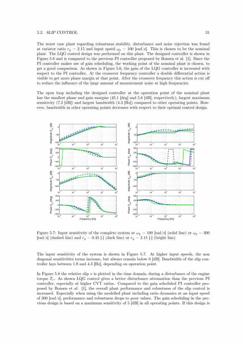
Figure 5.7: Input sensitivity of the complete system at ωp = 100 [rad/s] (solid line) or ωp = 300[rad/s] (dashed line) and rg = 0.45 [-] (dark line) or rg = 2.15 [-] (bright line)
The input sensitivity of the system is shown in Figure 5.7. At higher input speeds, the nondiagonal sensitivities terms increase, but always remain below 0 [dB]. Bandwidth of the slip con-troller lays between 1.9 and 4.3 [Hz], depending on operation point.
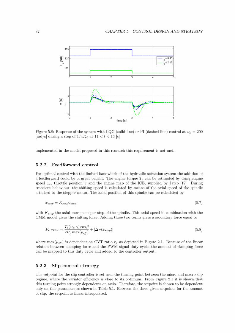
In Figure 5.8 the relative slip ν is plotted in the time domain, during a disturbance of the enginetorque Te. As shown LQG control gives a better disturbance attenuation than the previous PIcontroller, especially at higher CVT ratios. Compared to the gain scheduled PI controller pro-posed by Bonsen et al. [1], the overall plant performance and robustness of the slip control isincreased. Especially when using the modelled plant including ratio dynamics at an input speedof 300 [rad/s], performance and robustness drops to poor values. The gain scheduling in the pre-vious design is based on a maximum sensitivity of 5 [dB] in all operating points. If this design is
32 CHAPTER 5. CONTROL DESIGN AND STRATEGY
0 1 2 3 4 5
80
120
160
Te [N
m]
0 1 2 3 4 5
−5
0
5
time [s]
ν [%
]
rg = 0.45
rg = 2.15
Figure 5.8: Response of the system with LQG (solid line) or PI (dashed line) control at ωp = 200[rad/s] during a step of 1/4Te0 at 11 < t < 13 [s]
implemented in the model proposed in this research this requirement is not met.
5.2.2 Feedforward control
For optimal control with the limited bandwidth of the hydraulic actuation system the addition ofa feedforward could be of great benefit. The engine torque Te can be estimated by using enginespeed ωe, throttle position γ and the engine map of the ICE, supplied by Jatco [12]. Duringtransient behaviour, the shifting speed is calculated by means of the axial speed of the spindleattached to the stepper motor. The axial position of this spindle can be calculated by
xstep = Kstepustep (5.7)
with Kstep the axial movement per step of the spindle. This axial speed in combination with theCMM model gives the shifting force. Adding these two terms gives a secondary force equal to
Fs,FFW =Te(ωe, γ) cos β
2Rp max(µeff )+ |∆F (xstep)| (5.8)
where max(µeff ) is dependent on CVT ratio rg as depicted in Figure 2.1. Because of the linearrelation between clamping force and the PWM signal duty cycle, the amount of clamping forcecan be mapped to this duty cycle and added to the controller output.
5.2.3 Slip control strategy
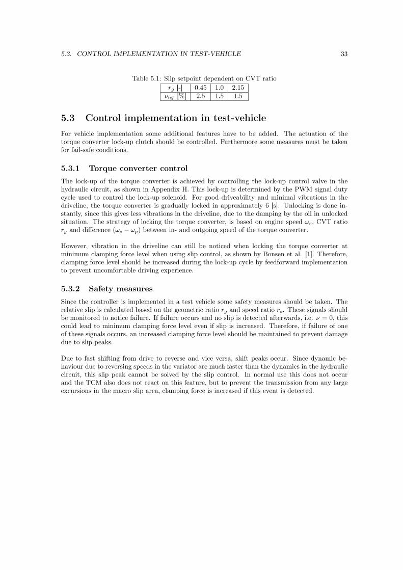
The setpoint for the slip controller is set near the turning point between the micro and macro slipregime, where the variator efficiency is close to its optimum. From Figure 2.1 it is shown thatthis turning point strongly dependents on ratio. Therefore, the setpoint is chosen to be dependentonly on this parameter as shown in Table 5.1. Between the three given setpoints for the amountof slip, the setpoint is linear interpolated.
5.3. CONTROL IMPLEMENTATION IN TEST-VEHICLE 33
Table 5.1: Slip setpoint dependent on CVT ratiorg [-] 0.45 1.0 2.15
νref [%] 2.5 1.5 1.5
5.3 Control implementation in test-vehicleFor vehicle implementation some additional features have to be added. The actuation of thetorque converter lock-up clutch should be controlled. Furthermore some measures must be takenfor fail-safe conditions.
5.3.1 Torque converter controlThe lock-up of the torque converter is achieved by controlling the lock-up control valve in thehydraulic circuit, as shown in Appendix H. This lock-up is determined by the PWM signal dutycycle used to control the lock-up solenoid. For good driveability and minimal vibrations in thedriveline, the torque converter is gradually locked in approximately 6 [s]. Unlocking is done in-stantly, since this gives less vibrations in the driveline, due to the damping by the oil in unlockedsituation. The strategy of locking the torque converter, is based on engine speed ωe, CVT ratiorg and difference (ωe − ωp) between in- and outgoing speed of the torque converter.
However, vibration in the driveline can still be noticed when locking the torque converter atminimum clamping force level when using slip control, as shown by Bonsen et al. [1]. Therefore,clamping force level should be increased during the lock-up cycle by feedforward implementationto prevent uncomfortable driving experience.
5.3.2 Safety measuresSince the controller is implemented in a test vehicle some safety measures should be taken. Therelative slip is calculated based on the geometric ratio rg and speed ratio rs. These signals shouldbe monitored to notice failure. If failure occurs and no slip is detected afterwards, i.e. ν = 0, thiscould lead to minimum clamping force level even if slip is increased. Therefore, if failure of oneof these signals occurs, an increased clamping force level should be maintained to prevent damagedue to slip peaks.
Due to fast shifting from drive to reverse and vice versa, shift peaks occur. Since dynamic be-haviour due to reversing speeds in the variator are much faster than the dynamics in the hydrauliccircuit, this slip peak cannot be solved by the slip control. In normal use this does not occurand the TCM also does not react on this feature, but to prevent the transmission from any largeexcursions in the macro slip area, clamping force is increased if this event is detected.

34 CHAPTER 5. CONTROL DESIGN AND STRATEGY
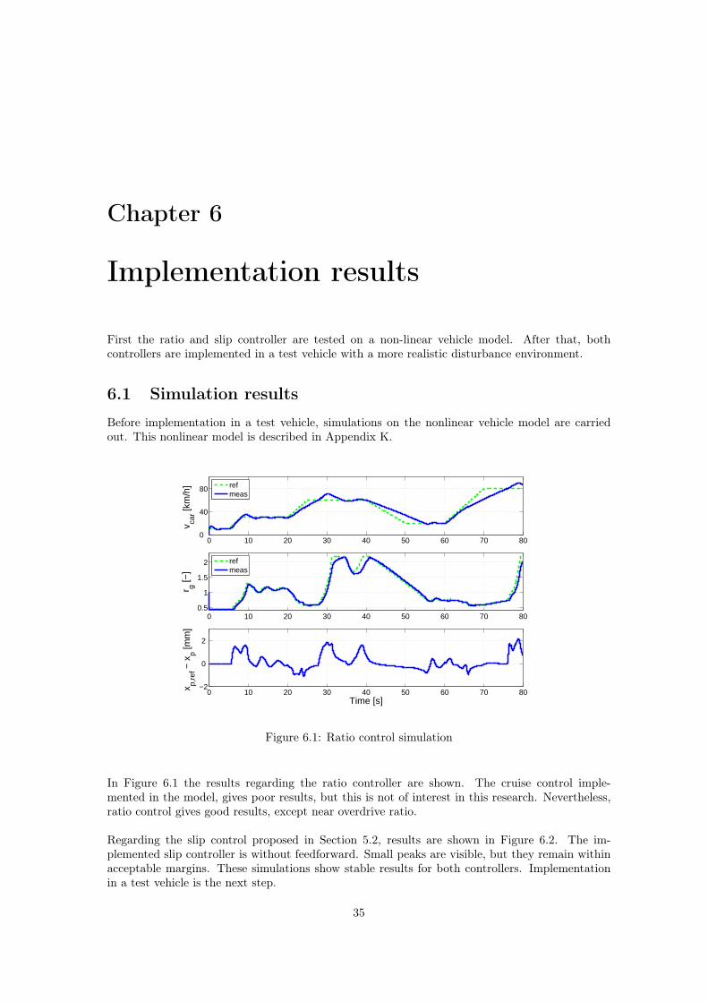
Chapter 6
Implementation results
First the ratio and slip controller are tested on a non-linear vehicle model. After that, bothcontrollers are implemented in a test vehicle with a more realistic disturbance environment.
6.1 Simulation results
Before implementation in a test vehicle, simulations on the nonlinear vehicle model are carriedout. This nonlinear model is described in Appendix K.
0 10 20 30 40 50 60 70 800
40
80
v car [k
m/h
]
0 10 20 30 40 50 60 70 800.5
1
1.5
2
r g [−]
0 10 20 30 40 50 60 70 80−2
0
2
Time [s]
x p,re
f − x
p [mm
]
refmeas
refmeas
Figure 6.1: Ratio control simulation
In Figure 6.1 the results regarding the ratio controller are shown. The cruise control imple-mented in the model, gives poor results, but this is not of interest in this research. Nevertheless,ratio control gives good results, except near overdrive ratio.
Regarding the slip control proposed in Section 5.2, results are shown in Figure 6.2. The im-plemented slip controller is without feedforward. Small peaks are visible, but they remain withinacceptable margins. These simulations show stable results for both controllers. Implementationin a test vehicle is the next step.
35
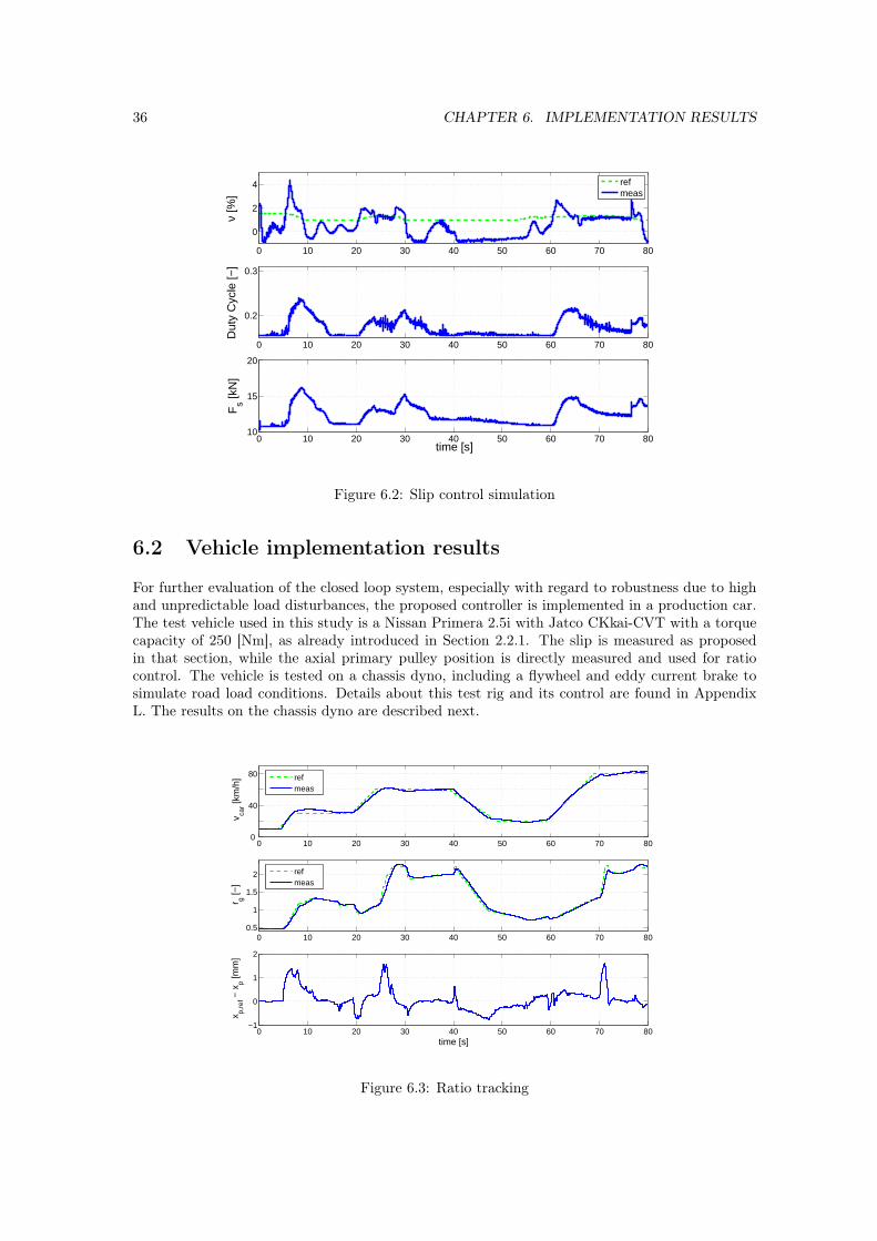
36 CHAPTER 6. IMPLEMENTATION RESULTS
0 10 20 30 40 50 60 70 80
0
2
4
ν [%
]
0 10 20 30 40 50 60 70 80
0.2
0.3
Dut
y C
ycle
[−]
0 10 20 30 40 50 60 70 8010
15
20
time [s]
Fs [k
N]
refmeas
Figure 6.2: Slip control simulation
6.2 Vehicle implementation results
For further evaluation of the closed loop system, especially with regard to robustness due to highand unpredictable load disturbances, the proposed controller is implemented in a production car.The test vehicle used in this study is a Nissan Primera 2.5i with Jatco CKkai-CVT with a torquecapacity of 250 [Nm], as already introduced in Section 2.2.1. The slip is measured as proposedin that section, while the axial primary pulley position is directly measured and used for ratiocontrol. The vehicle is tested on a chassis dyno, including a flywheel and eddy current brake tosimulate road load conditions. Details about this test rig and its control are found in AppendixL. The results on the chassis dyno are described next.
0 10 20 30 40 50 60 70 800
40
80
v car [k
m/h
]
0 10 20 30 40 50 60 70 800.5
1
1.5
2
r g [−]
0 10 20 30 40 50 60 70 80−1
0
1
2
x p,re
f − x
p [mm
]
time [s]
refmeas
refmeas
Figure 6.3: Ratio tracking
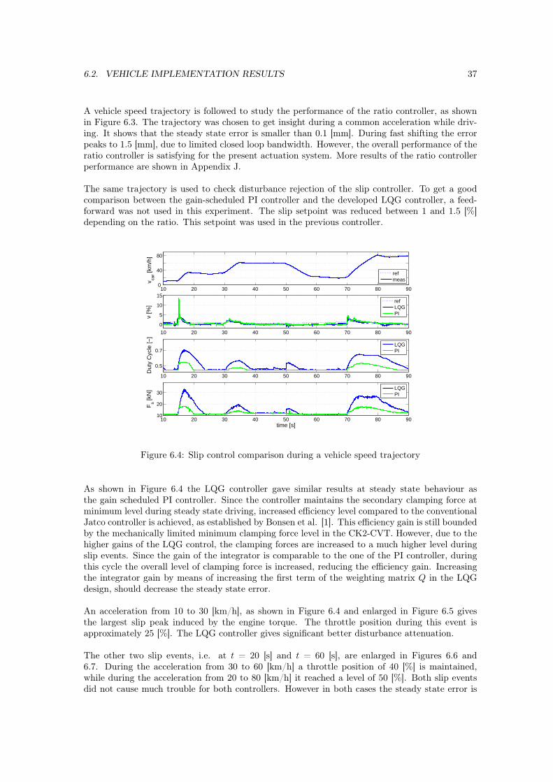
6.2. VEHICLE IMPLEMENTATION RESULTS 37
A vehicle speed trajectory is followed to study the performance of the ratio controller, as shownin Figure 6.3. The trajectory was chosen to get insight during a common acceleration while driv-ing. It shows that the steady state error is smaller than 0.1 [mm]. During fast shifting the errorpeaks to 1.5 [mm], due to limited closed loop bandwidth. However, the overall performance of theratio controller is satisfying for the present actuation system. More results of the ratio controllerperformance are shown in Appendix J.
The same trajectory is used to check disturbance rejection of the slip controller. To get a goodcomparison between the gain-scheduled PI controller and the developed LQG controller, a feed-forward was not used in this experiment. The slip setpoint was reduced between 1 and 1.5 [%]depending on the ratio. This setpoint was used in the previous controller.
10 20 30 40 50 60 70 80 900
40
80
v car [k
m/h
]
10 20 30 40 50 60 70 80 90
0
5
10
15
ν [%
]
10 20 30 40 50 60 70 80 90
0.5
0.7
Dut
y C
ycle
[−]
10 20 30 40 50 60 70 80 9010
20
30
time [s]
Fs [k
N]
refmeas
refLQGPI
LQGPI
LQGPI
Figure 6.4: Slip control comparison during a vehicle speed trajectory
As shown in Figure 6.4 the LQG controller gave similar results at steady state behaviour asthe gain scheduled PI controller. Since the controller maintains the secondary clamping force atminimum level during steady state driving, increased efficiency level compared to the conventionalJatco controller is achieved, as established by Bonsen et al. [1]. This efficiency gain is still boundedby the mechanically limited minimum clamping force level in the CK2-CVT. However, due to thehigher gains of the LQG control, the clamping forces are increased to a much higher level duringslip events. Since the gain of the integrator is comparable to the one of the PI controller, duringthis cycle the overall level of clamping force is increased, reducing the efficiency gain. Increasingthe integrator gain by means of increasing the first term of the weighting matrix Q in the LQGdesign, should decrease the steady state error.
An acceleration from 10 to 30 [km/h], as shown in Figure 6.4 and enlarged in Figure 6.5 givesthe largest slip peak induced by the engine torque. The throttle position during this event isapproximately 25 [%]. The LQG controller gives significant better disturbance attenuation.
The other two slip events, i.e. at t = 20 [s] and t = 60 [s], are enlarged in Figures 6.6 and6.7. During the acceleration from 30 to 60 [km/h] a throttle position of 40 [%] is maintained,while during the acceleration from 20 to 80 [km/h] it reached a level of 50 [%]. Both slip eventsdid not cause much trouble for both controllers. However in both cases the steady state error is
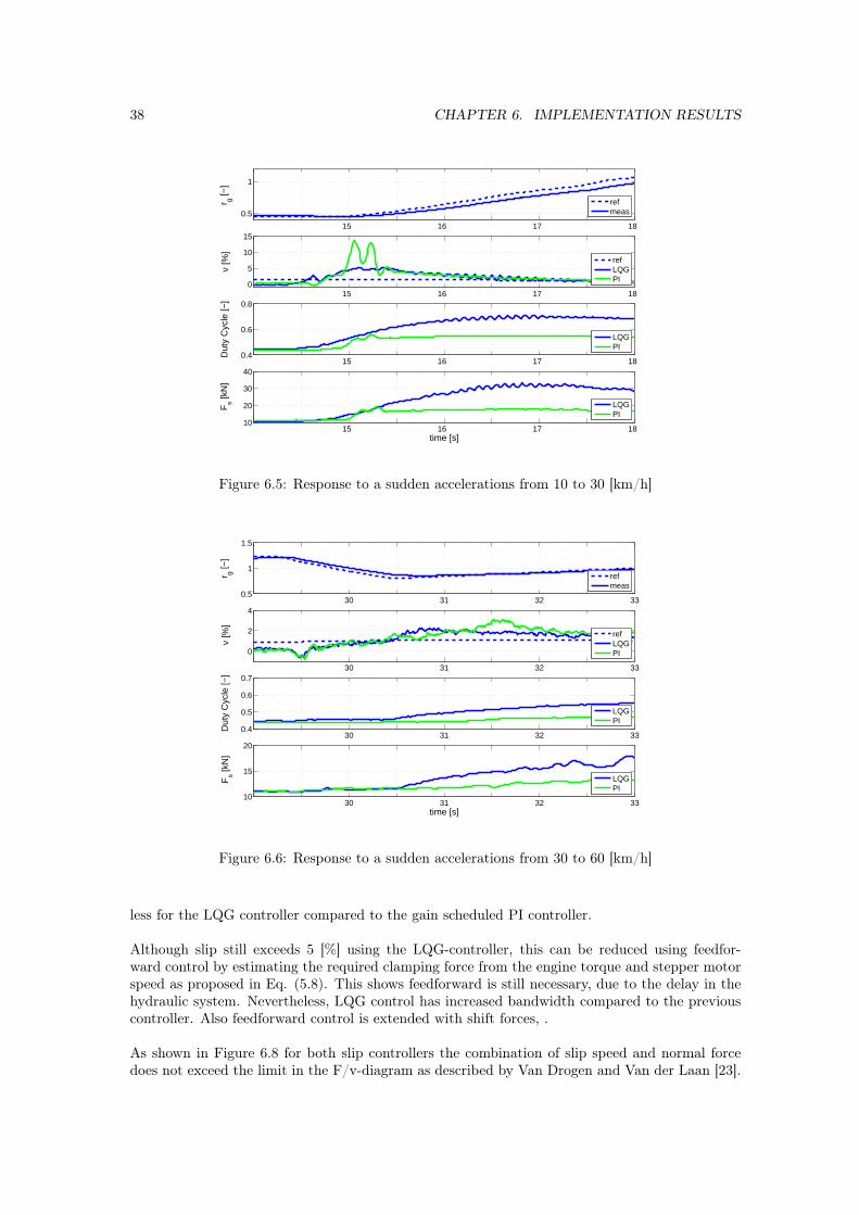
38 CHAPTER 6. IMPLEMENTATION RESULTS
15 16 17 18
0.5
1
r g [−]
15 16 17 18 0
5
10
15
ν [%
]
15 16 17 18 0.4
0.6
0.8
Dut
y C
ycle
[−]
15 16 17 18 10
20
30
40
time [s]
Fs [k
N]
refmeas
LQGPI
LQGPI
refLQGPI
Figure 6.5: Response to a sudden accelerations from 10 to 30 [km/h]
30 31 32 330.5
1
1.5
r g [−]
30 31 32 33
0
2
4
ν [%
]
30 31 32 330.4
0.5
0.6
0.7
Dut
y C
ycle
[−]
30 31 32 3310
15
20
time [s]
Fs [k
N]
refmeas
refLQGPI
LQGPI
LQGPI
Figure 6.6: Response to a sudden accelerations from 30 to 60 [km/h]
less for the LQG controller compared to the gain scheduled PI controller.
Although slip still exceeds 5 [%] using the LQG-controller, this can be reduced using feedfor-ward control by estimating the required clamping force from the engine torque and stepper motorspeed as proposed in Eq. (5.8). This shows feedforward is still necessary, due to the delay in thehydraulic system. Nevertheless, LQG control has increased bandwidth compared to the previouscontroller. Also feedforward control is extended with shift forces, .
As shown in Figure 6.8 for both slip controllers the combination of slip speed and normal forcedoes not exceed the limit in the F/v-diagram as described by Van Drogen and Van der Laan [23].
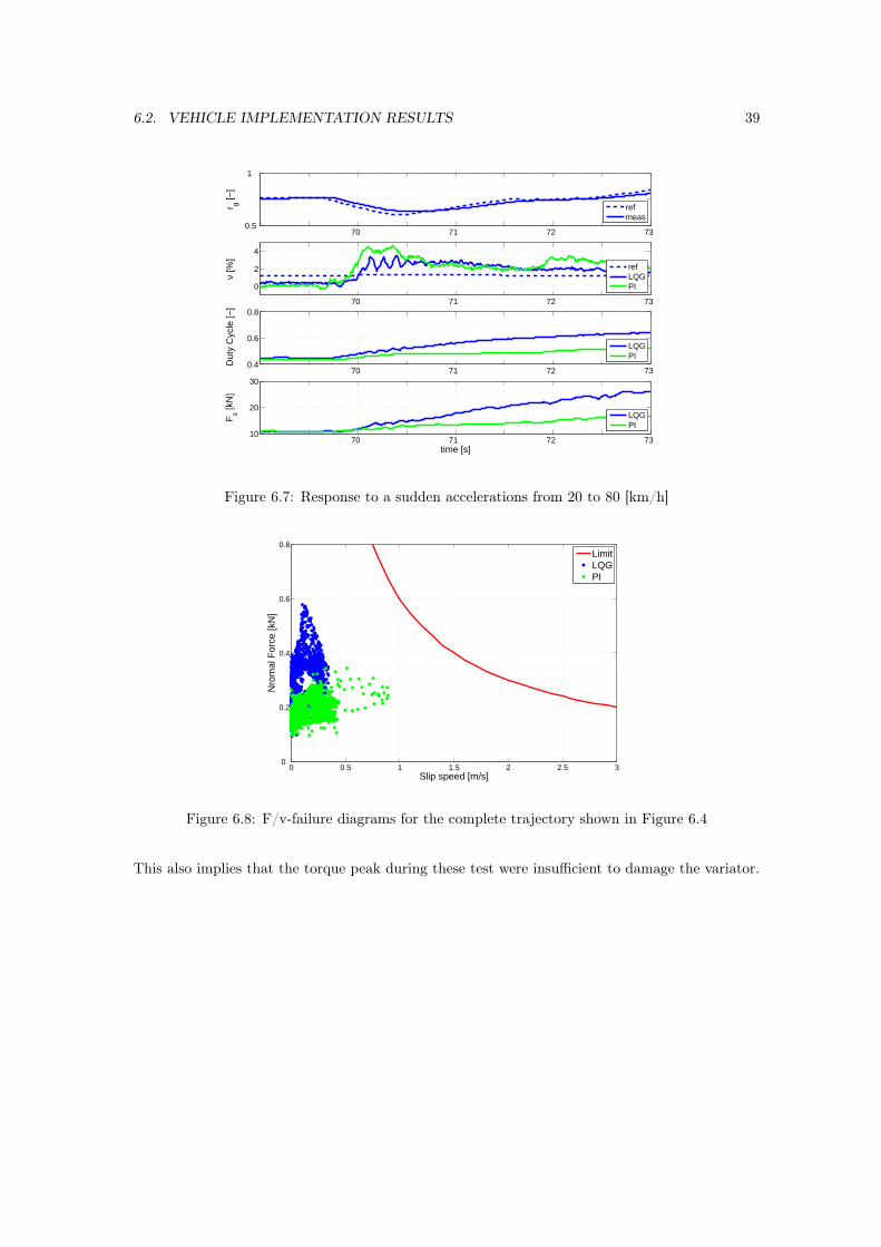
6.2. VEHICLE IMPLEMENTATION RESULTS 39
70 71 72 73 0.5
1
r g [−]
70 71 72 73
0
2
4
ν [%
]
70 71 72 73 0.4
0.6
0.8
Dut
y C
ycle
[−]
70 71 72 73 10
20
30
time [s]
Fs [k
N]
refmeas
refLQGPI
LQGPI
LQGPI
Figure 6.7: Response to a sudden accelerations from 20 to 80 [km/h]
0 0.5 1 1.5 2 2.5 30
0.2
0.4
0.6
0.8
Slip speed [m/s]
Nro
mal
For
ce [k
N]
LimitLQGPI
Figure 6.8: F/v-failure diagrams for the complete trajectory shown in Figure 6.4
This also implies that the torque peak during these test were insufficient to damage the variator.

40 CHAPTER 6. IMPLEMENTATION RESULTS
Chapter 7
Conclusions and recommendations
7.1 Conclusions• Different shift models in the literature are investigated. The best suitable models considering
this pushbelt type of CVT and slip control technique are validated and compared. As a resultthe CMM model gave the best agreement to reality and is therefore used in the rest of thevariator modelling.
• A more complete model of the variator considering slip and ratio dynamics, as well as thehydraulic actuation dynamics of both line and primary pressure, are derived. Also interactionbetween both slip and ratio dynamics is analysed, leading to the possibility of decentralizedcontrol design.
• The newly developed slip controller based on LQG control design, gives better disturbanceattenuation and increased bandwidth compared to the previous designed PI controller, whilethe improved efficiency level at steady state behaviour is maintained.
7.2 Recommendations• More principle work on the friction behaviour between elements of the pushbelt and between
element and bands could be of interest to improve the shift model. Especially at low torqueratios and low clamping force levels the CMM model does not give good agreement to reality.Also the additional dynamics in the production CVT compared to a single variator can beof interest to declare the anti-symmetry between up- and downshifting.
• Since slip control technique is applied, leading to slip in tangential direction, the influence ofslip in radial direction should be further analysed. This should lead to a better identificationof slip behaviour during shifting, improving the modelling of the variator regarding slipbetween pulleys and belt.
• With the present modelling, the optimal performance of the slip control is achieved withthe present hydraulic actuation system. Adapting the hydraulic system for best possiblecontrol performance and robustness, instead of adapting the control to the hydraulics at theCK2-CVT, is preferred.
• Research on the long-term effects with respect to variator damage while using slip control isstill necessary, to validate the use of this control technique in pushbelt variators.
41

42 CHAPTER 7. CONCLUSIONS AND RECOMMENDATIONS
Bibliography
[1] B. Bonsen, T.W.G.L. Klaassen, R.J. Pulles, S.W.H. Simons, M. Steinbuch, and P.A. Veen-huizen. Performance optimization of the push-belt CVT by variator slip control. Journal ofvehicle design, 2005.
[2] B. Bonsen, T.W.G.L. Klaassen, K.G.O. van de Meerakker, P.A. Veenhuizen, and M. Stein-buch. Measurement and control of slip in a continuously variable transmission. In AustraliaIFAC, Sydney, editor, Mechatronics 2004, pages 43–48, 2004.
[3] B. Bonsen, T.W.G.L. Klaassen, K.G.O. van de Meerakker, P.A. Veenhuizen, and M. Stein-buch. Modelling slip- and creepmode shift speed characteristics of a push-belt type continu-ously variable transmission. In International Continuously Variable and Hybrid TransmissionCongress, Frank, Davis, CA, United States, 2004.
[4] B. Bonsen, P.A. Veenhuizen, and M. Steinbuch. CVT ratio control strategy optimization. InUnited States IEEE, Chicago, editor, VPPC, 2005.
[5] G. Carbone, L. Mangialardi, B. Bonsen, C. Tursi, and P.A. Veenhuizen. CVT dynamics:Theory and experiments. Mechanism and Machine Theory. in press.
[6] G. Carbone, L. Mangialardi, and G. Mantriota. EHL visco-plastic friction model in CVTshifting behaviour. Journal of vehicle design, 32(3/4):332–357, 2003.
[7] G. Carbone, L. Mangialardi, and G. Mantriota. The influence of pulley deformations on theshifting mechanism of metal belt CVT. Journal of mechanical design, 2005.
[8] T. Ide, H. Uchiyama, and R. Kataoka. Simulation approach to the effect of the ratio changingspeed of a metal V-belt CVT on the vehicle response. Vehicle System Dynamics, 24:377–388,1995.
[9] T. Ide, H. Uchiyama, and R. Kataoka. Experimental investigation on shift speed character-istics of a metal V-belt CVT. JSAE no 96360330, 1996.
[10] T.W.G.L. Klaassen and M. Steinbuch. Identification and control of the Empact CVT. Sub-mitted to IEEE Transactions on Control Systems Technology, May 2006.
[11] D. Kobayashi, Y. Mabuchi, and Y. Katoh. A study on the torque capacity of a metal pushingV-belt for CVTs. SAE technical paper series, no 980822, 1998.
[12] K. Michael. Jatco Europe GmbH. Personal contact.
[13] T. Fujii S. Kanehara O. Fujimura, S. Kuwabara. Study on shifting mechanisms of metalpushing V-belt type CVT - dealing with shifting rate and mean coefficient of friction. JSAEno 9838363, 1998.
[14] M.F. Oudijk. Application of a TNO-MACS system on a Nissan CK2-CVT. Dct-nr. 2003.76,TU/e, Eindhoven, 2003.
43
44 BIBLIOGRAPHY
[15] H. Peeters. Design and realization of a spin loss transmission test rig. Master’s thesis, TU/e,Eindhoven, 2001.
[16] R.J. Pulles. Slip controller design and implementation in a continuously variable transmission.Dct-nr. 2004.102, TU/e, Eindhoven, 2004.
[17] T. Fujii S. Kanehara R. Kataoke, K. Okubo. A study on a metal pushing V-belt type CVT- a novel approach to characterize the friction between blocks and a pulley, and shiftingmechanisms. SAE no. 2002-01-0697, 2002.
[18] J. Rijnsdorp. Interaction in two variable control systems for distillation columns. Automatica,1:15–28, 1965.
[19] H. Sattler. Efficiency of metal chain and V-belt CVT. In Proceedings CVT’99 Congress,Eindhoven, The Netherlands, pages 99–104, 1999.
[20] E. Shafai, M. Simons, U. Neff, and P. Geering. Model of a continuously variable transmission.Vehicle System Dynamics, 1995.
[21] S. Skogestad and I. Postlethwaite. Multivariable feedback control. Wiley, 1996.
[22] P. Tenberge. Efficiency of chain-CVTs at constant and variable ratio. In 2004 InternationalContinuously Variable and Hybrid Transmission Congress, UC Davis, United States, 2004.
[23] M. van Drogen and M. van der Laan. Determination of variator robustness under macro slipconditions for a push belt CVT. SAE world congress 2004, 2004.
[24] B. Vroemen. Component control for the zero inertia powertrain. Technische UniversiteitEindhoven, 2001.
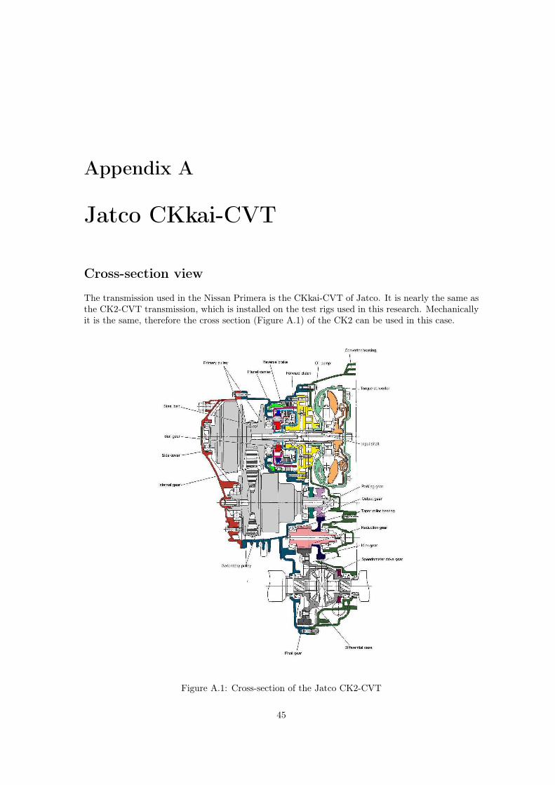
Appendix A
Jatco CKkai-CVT
Cross-section view
The transmission used in the Nissan Primera is the CKkai-CVT of Jatco. It is nearly the same asthe CK2-CVT transmission, which is installed on the test rigs used in this research. Mechanicallyit is the same, therefore the cross section (Figure A.1) of the CK2 can be used in this case.
Figure A.1: Cross-section of the Jatco CK2-CVT
45
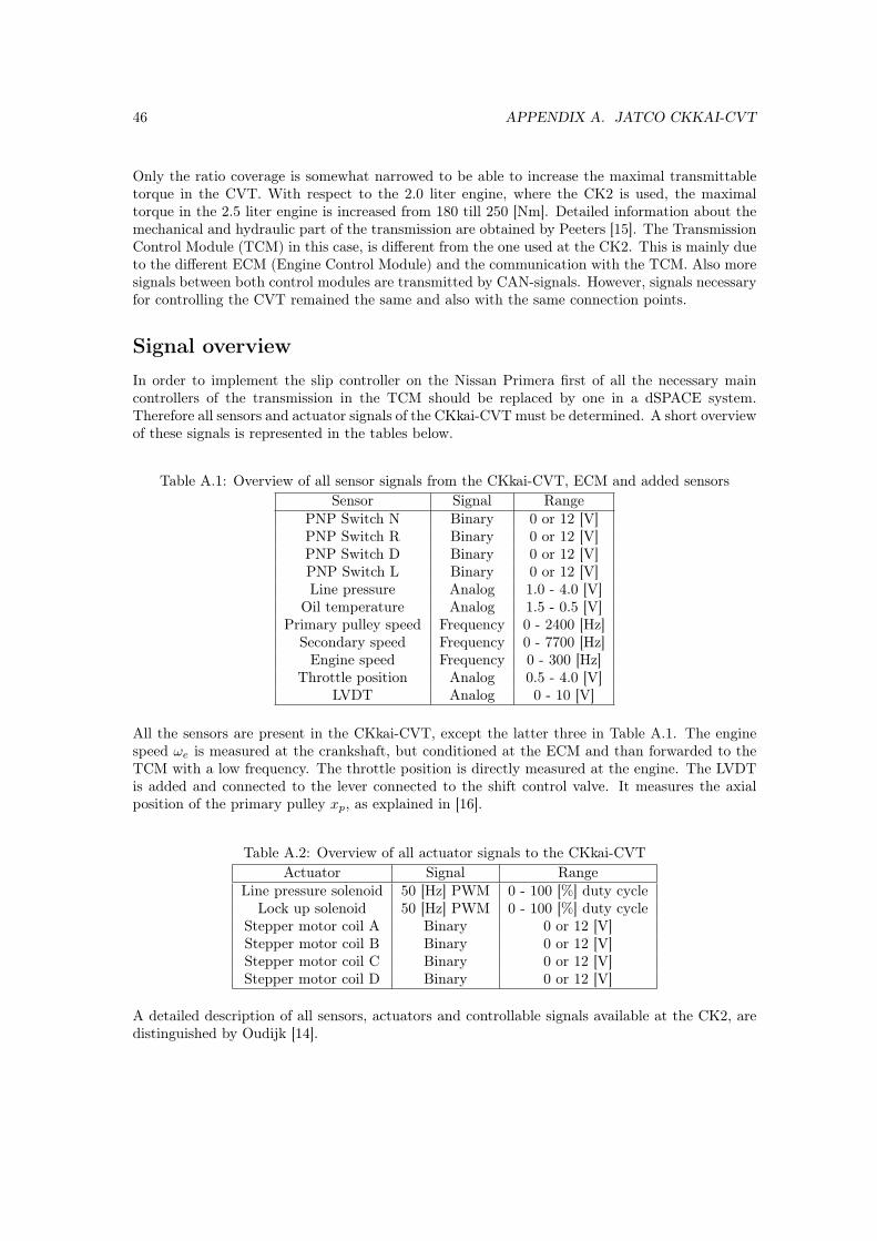
46 APPENDIX A. JATCO CKKAI-CVT
Only the ratio coverage is somewhat narrowed to be able to increase the maximal transmittabletorque in the CVT. With respect to the 2.0 liter engine, where the CK2 is used, the maximaltorque in the 2.5 liter engine is increased from 180 till 250 [Nm]. Detailed information about themechanical and hydraulic part of the transmission are obtained by Peeters [15]. The TransmissionControl Module (TCM) in this case, is different from the one used at the CK2. This is mainly dueto the different ECM (Engine Control Module) and the communication with the TCM. Also moresignals between both control modules are transmitted by CAN-signals. However, signals necessaryfor controlling the CVT remained the same and also with the same connection points.
Signal overviewIn order to implement the slip controller on the Nissan Primera first of all the necessary maincontrollers of the transmission in the TCM should be replaced by one in a dSPACE system.Therefore all sensors and actuator signals of the CKkai-CVT must be determined. A short overviewof these signals is represented in the tables below.
Table A.1: Overview of all sensor signals from the CKkai-CVT, ECM and added sensorsSensor Signal Range
PNP Switch N Binary 0 or 12 [V]PNP Switch R Binary 0 or 12 [V]PNP Switch D Binary 0 or 12 [V]PNP Switch L Binary 0 or 12 [V]Line pressure Analog 1.0 - 4.0 [V]
Oil temperature Analog 1.5 - 0.5 [V]Primary pulley speed Frequency 0 - 2400 [Hz]
Secondary speed Frequency 0 - 7700 [Hz]Engine speed Frequency 0 - 300 [Hz]
Throttle position Analog 0.5 - 4.0 [V]LVDT Analog 0 - 10 [V]
All the sensors are present in the CKkai-CVT, except the latter three in Table A.1. The enginespeed ωe is measured at the crankshaft, but conditioned at the ECM and than forwarded to theTCM with a low frequency. The throttle position is directly measured at the engine. The LVDTis added and connected to the lever connected to the shift control valve. It measures the axialposition of the primary pulley xp, as explained in [16].
Table A.2: Overview of all actuator signals to the CKkai-CVTActuator Signal Range
Line pressure solenoid 50 [Hz] PWM 0 - 100 [%] duty cycleLock up solenoid 50 [Hz] PWM 0 - 100 [%] duty cycle
Stepper motor coil A Binary 0 or 12 [V]Stepper motor coil B Binary 0 or 12 [V]Stepper motor coil C Binary 0 or 12 [V]Stepper motor coil D Binary 0 or 12 [V]
A detailed description of all sensors, actuators and controllable signals available at the CK2, aredistinguished by Oudijk [14].
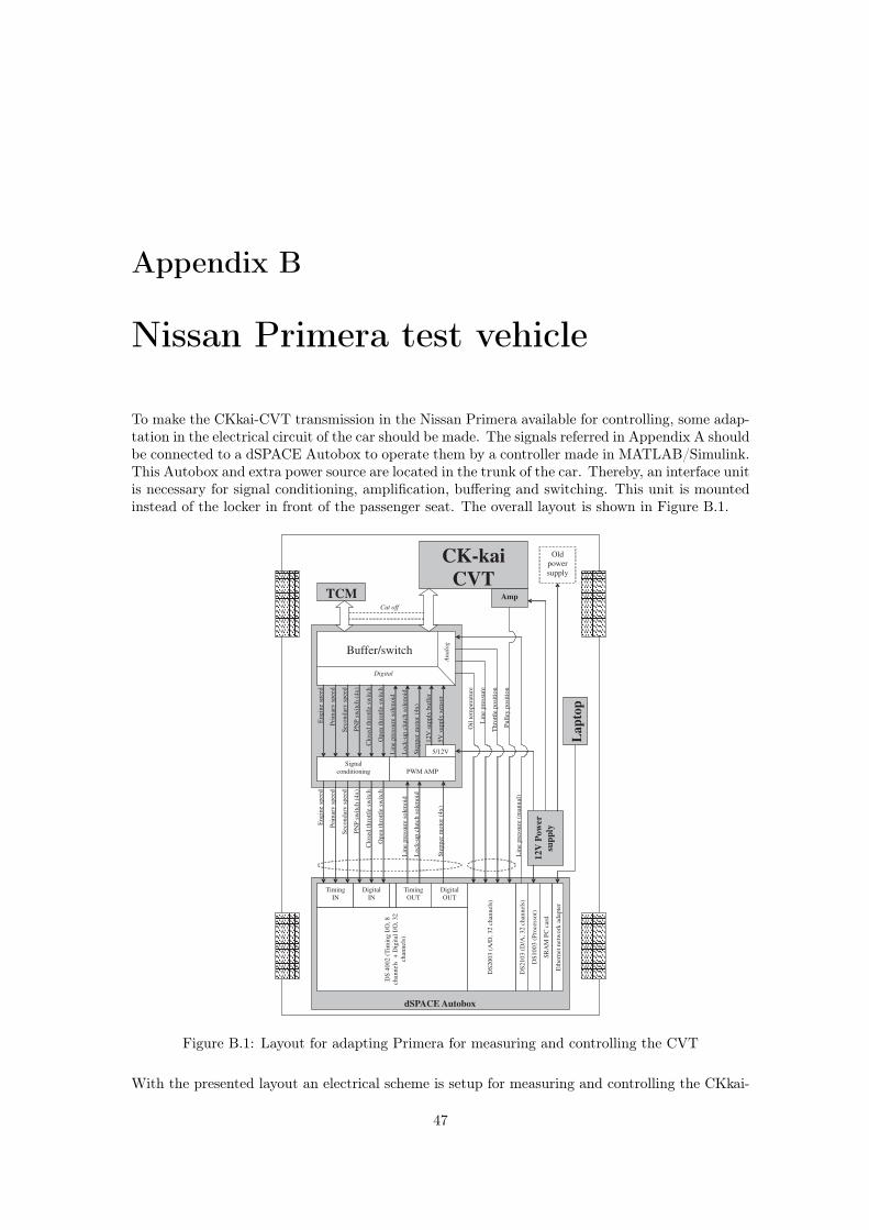
Appendix B
Nissan Primera test vehicle
To make the CKkai-CVT transmission in the Nissan Primera available for controlling, some adap-tation in the electrical circuit of the car should be made. The signals referred in Appendix A shouldbe connected to a dSPACE Autobox to operate them by a controller made in MATLAB/Simulink.This Autobox and extra power source are located in the trunk of the car. Thereby, an interface unitis necessary for signal conditioning, amplification, buffering and switching. This unit is mountedinstead of the locker in front of the passenger seat. The overall layout is shown in Figure B.1.
dSPACE Autobox
12V
Pow
er
sup
ply
CK-kai
CVTTCM
DS
21
03
(D/A
,32
chan
nel
s)
Eth
ern
etn
etw
ork
adap
ter
DS
40
02
(Tim
ing
I/O
,8
chan
nel
s+
Dig
ital
I/O
,32
chan
nel
s)
DS
20
03
(A/D
,32
chan
nel
s)
DS
10
03
(Pro
cess
or)
SR
AM
PC
card
Signal
conditioning
Buffer/switch
En
gin
esp
eed
Pri
mar
ysp
eed
Sec
on
dar
ysp
eed
Op
enth
rott
lesw
itch
Clo
sed
thro
ttle
swit
ch
PN
Psw
itch
(4x
)
PWM AMP
5/12VSte
pp
erm
oto
r(4
x)
12
Vsu
pp
lyb
uff
er
Lo
ck-u
pcl
utc
hso
leno
id
5V
sup
ply
sen
sor
Lin
ep
ress
ure
sole
no
id
Timing
IN
Digital
IN
Digital
OUT
Timing
OUT
En
gin
esp
eed
Pri
mar
ysp
eed
Sec
on
dar
ysp
eed
PN
Psw
itch
(4x
)
Clo
sed
thro
ttle
swit
ch
Op
enth
rott
lesw
itch
La
pto
p
Pu
lley
po
siti
on
Lin
ep
ress
ure
sole
no
id
Lo
ck-u
pcl
utc
hso
leno
id
Ste
pp
erm
oto
r(4
x)
Cut off
Th
rott
lep
osi
tio
n
Lin
ep
ress
ure
Oil
tem
per
atu
re
Amp
Lin
ep
ress
ure
(man
ual
)
Digital
An
alo
g
Old
power
supply
Figure B.1: Layout for adapting Primera for measuring and controlling the CVT
With the presented layout an electrical scheme is setup for measuring and controlling the CKkai-
47
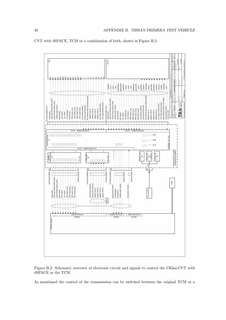
48 APPENDIX B. NISSAN PRIMERA TEST VEHICLE
CVT with dSPACE, TCM or a combination of both, shown in Figure B.2.
DA
TE21
-9-2
004
DR
AW
N B
Y CTD
KR
UY
S
FILE
NA
ME
PR
IME
RA
.VS
D
TIT
LE
FULL
FIL
EN
AM
EM
:\PR
OJE
KTEN
\PR
IMER
A\VI
SIO
\PR
IMER
A.VS
D
OR
DE
R N
R.
SU
BJE
CT
LOC
ATI
ON
CO
MP
AN
Y
13
DE
PA
RTM
EN
TG
emee
nsch
appe
lijke
Tec
hnis
che
Die
nst
RE
V AS
UB
JEC
T10
0012
05D
ES
CR
IPTI
ON
BLO
KS
CH
EM
A P
RIM
ER
AD
ATE
00-0
0-20
00A
PR
OV
ED
BY
LAS
T R
EV
ISIO
N (
for H
isto
ry s
ee “R
evis
ion
Log”
)
wid
e op
en th
rottl
e po
sitio
n sw
itch
Lapt
op
CK-
kai
TCM
dSPA
CE
Auto
box
clos
ed th
rottl
e po
sitio
n sw
itch
engi
ne s
peed
sec.
spe
ed
prim
. spe
ed
PN
P s
witc
h L
pos
lock
-up
clut
ch s
olen
oid
line
pres
sure
sol
enoi
d
step
per m
otor
A
oil t
empe
ratu
re
PN
P s
witc
h L
pos
lock
-up
clut
ch s
olen
oid
line
pres
sure
sol
enoi
d
step
per m
otor
A
wid
e op
en th
rottl
e po
sitio
n sw
itch
clos
ed th
rottl
e po
sitio
n sw
itch
thro
ttle
posi
tion
sens
or
engi
ne s
peed
sec.
spe
ed
prim
. spe
ed
line
pres
sure
wid
e op
en th
rottl
e po
sitio
n sw
itch
clos
ed th
rottl
e po
sitio
n sw
itch
thro
ttle
posi
tion
sens
or
engi
ne s
peed
lock
-up
clut
ch s
olen
oid
line
pres
sure
sol
enoi
d
step
per m
otor
A
sec.
spe
ed
prim
. spe
ed
oil t
empe
ratu
re
PN
P s
witc
h L
pos
41 39 2938 47 31 3211 12 20 21
step
per m
otor
B
step
per m
otor
C
step
per m
otor
Dst
eppe
r mot
or B
step
per m
otor
C
step
per m
otor
D
PN
P s
witc
h D
pos
PN
P s
witc
h R
pos
PN
P s
witc
h N
pos
27 34 35 36
PN
P s
witc
h D
pos
PN
P s
witc
h R
pos
PN
P s
witc
h N
pos
line
pres
sure
step
per m
otor
B
step
per m
otor
C
step
per m
otor
D
PN
P s
witc
h D
pos
PN
P s
witc
h R
pos
PN
P s
witc
h N
pos
37
25 POLIGE SUBDM XC102
25 POLIGE SUBDM XC101
Switc
hed
Sign
als
Buffe
red
Sign
als
25 POLIGE SUBDF XC100
46
line
pres
sure
sol
enoi
d dr
oppi
ng re
sist
or2
+5V
sup
ply
thro
ttle
sens
or
+5V
supp
ly p
ress
ure
sens
or
BUFF
ER/S
WIT
CH
U1
oil t
empe
ratu
re
line
pres
sure
thro
ttle
posi
tion
sens
or
SIG
NAL
CO
ND
ITIO
NIN
G
U2
PW
M-A
MP
U3
INTE
RFA
CEK
AST
ON
DER
DAS
HBO
ARD
PR
IMER
A
line
pres
sure
man
ual
DC
-DC
+12
VU4
DC
-DC
+5V
U5FU
SE 3
A
DC
-DC
-5V
U6
Switc
hed
Sign
al
Accu
12V
DC
brak
e sw
itch
brak
e sw
itch
brak
e sw
itch
45 nc nc
Buffe
red
Sign
als
S1 1XS2 4X
S3 7X
line
pres
sure
sol
enoi
d dr
oppi
ng re
sist
or
VOED
ING
: +5V
+12
V
+5V
+12
V
+5V
-5V
+5V
sup
ply
thro
ttle
sens
or
+5V
supp
ly p
ress
ure
sens
or
pulle
y po
sitio
n se
nsor
25 P
OLI
GE
SUBD
M X
102
25 P
OLI
GE
SUBD
M X
101
25 P
OLI
GE
SUBD
F X1
00
pulle
y po
sitio
n se
nsor
pulle
y po
sitio
n se
nsor
+12
V su
pply
50 POLIGE SUBDF 50 POLIGE SUBDM 50 POLIGE SUBDF
X1Q
1
25 P
OLI
GE
SUBD
M X
102
15 P
OLI
GE
SUBD
M X
103
red/
gree
n
colo
r ?
colo
r ?
colo
r ?
red/
brow
n
grey
bleu
/ora
nge
gree
n/ye
llow
gree
n/re
d
brow
n
whi
te
red/
bleu
blue
whi
te/g
reen
gree
n/w
hite
gree
n
red/
whi
te
grey
/red
pink
/bla
ck
purp
le
bleu
/whi
te
bleu
/yel
low
pink
/ble
u
red/
blac
k
Twis
ted
Pair
2x8x
0,22
DS2103DS2003DS4002
grou
nd p
in 2
5 !
Figure B.2: Schematic overview of electronic circuit and signals to control the CKkai-CVT withdSPACE or the TCM
As mentioned the control of the transmission can be switched between the original TCM or a
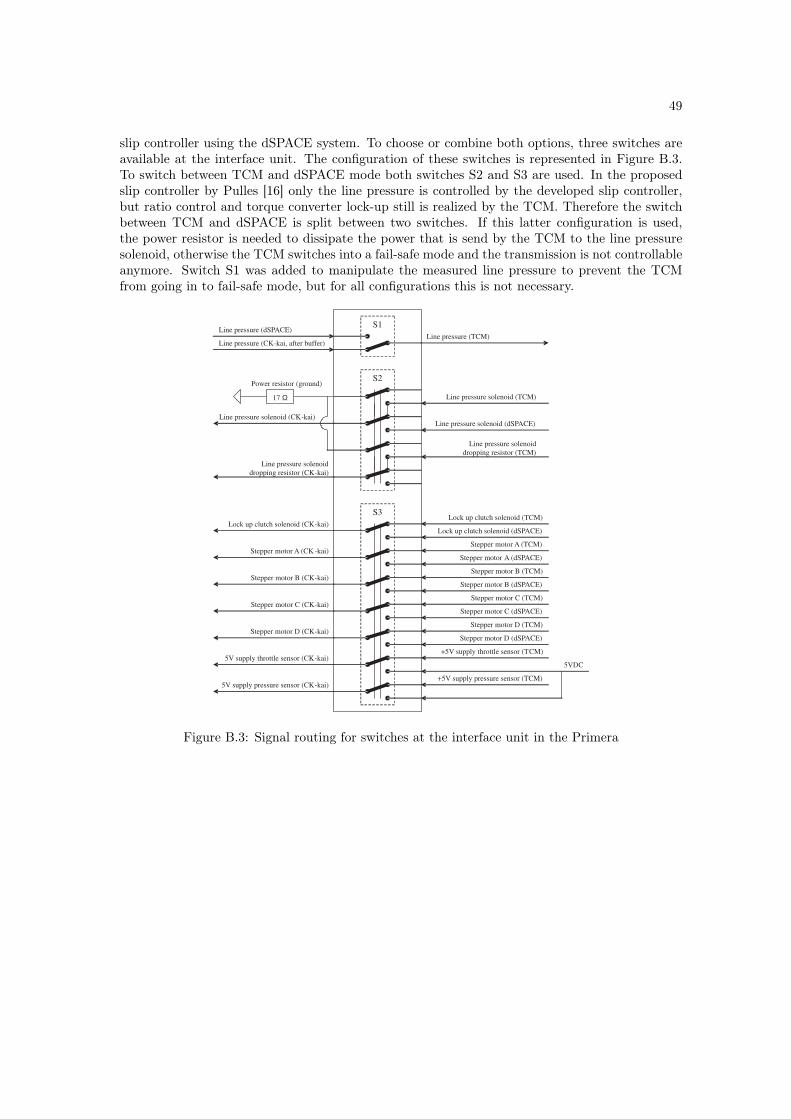
49
slip controller using the dSPACE system. To choose or combine both options, three switches areavailable at the interface unit. The configuration of these switches is represented in Figure B.3.To switch between TCM and dSPACE mode both switches S2 and S3 are used. In the proposedslip controller by Pulles [16] only the line pressure is controlled by the developed slip controller,but ratio control and torque converter lock-up still is realized by the TCM. Therefore the switchbetween TCM and dSPACE is split between two switches. If this latter configuration is used,the power resistor is needed to dissipate the power that is send by the TCM to the line pressuresolenoid, otherwise the TCM switches into a fail-safe mode and the transmission is not controllableanymore. Switch S1 was added to manipulate the measured line pressure to prevent the TCMfrom going in to fail-safe mode, but for all configurations this is not necessary.
S1
S2
S3
Line pressure solenoid (CK-kai)
5V supply pressure sensor (CK-kai)
Line pressure solenoid
dropping resistor (CK-kai)
Stepper motor C (CK-kai)
Stepper motor B (CK-kai)
Lock up clutch solenoid (CK-kai)
Stepper motor D (CK-kai)
5V supply throttle sensor (CK-kai)
Line pressure (CK-kai, after buffer)
Stepper motor A (CK -kai)
Line pressure (TCM)
Line pressure solenoid (TCM)
Line pressure solenoid (dSPACE)
Line pressure solenoid
dropping resistor (TCM)
Lock up clutch solenoid (TCM)
Stepper motor A (TCM)
Stepper motor A (dSPACE)
Lock up clutch solenoid (dSPACE)
Stepper motor B (TCM)
Stepper motor B (dSPACE)
Stepper motor C (TCM)
Stepper motor C (dSPACE)
Stepper motor D (TCM)
Stepper motor D (dSPACE)
Line pressure (dSPACE)
+5V supply throttle sensor (TCM)
5VDC
+5V supply pressure sensor (TCM)
17 Ω
Power resistor (ground)
Figure B.3: Signal routing for switches at the interface unit in the Primera

50 APPENDIX B. NISSAN PRIMERA TEST VEHICLE
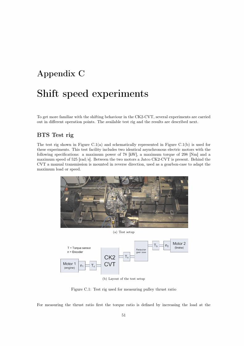
Appendix C
Shift speed experiments
To get more familiar with the shifting behaviour in the CK2-CVT, several experiments are carriedout in different operation points. The available test rig and the results are described next.
BTS Test rigThe test rig shown in Figure C.1(a) and schematically represented in Figure C.1(b) is used forthese experiments. This test facility includes two identical asynchronous electric motors with thefollowing specifications: a maximum power of 78 [kW], a maximum torque of 298 [Nm] and amaximum speed of 525 [rad/s]. Between the two motors a Jatco CK2-CVT is present. Behind theCVT a manual transmission is mounted in reverse direction, used as a gearbox-case to adapt themaximum load or speed.
(a) Test setup
(b) Layout of the test setup
Figure C.1: Test rig used for measuring pulley thrust ratio
For measuring the thrust ratio first the torque ratio is defined by increasing the load at the
51
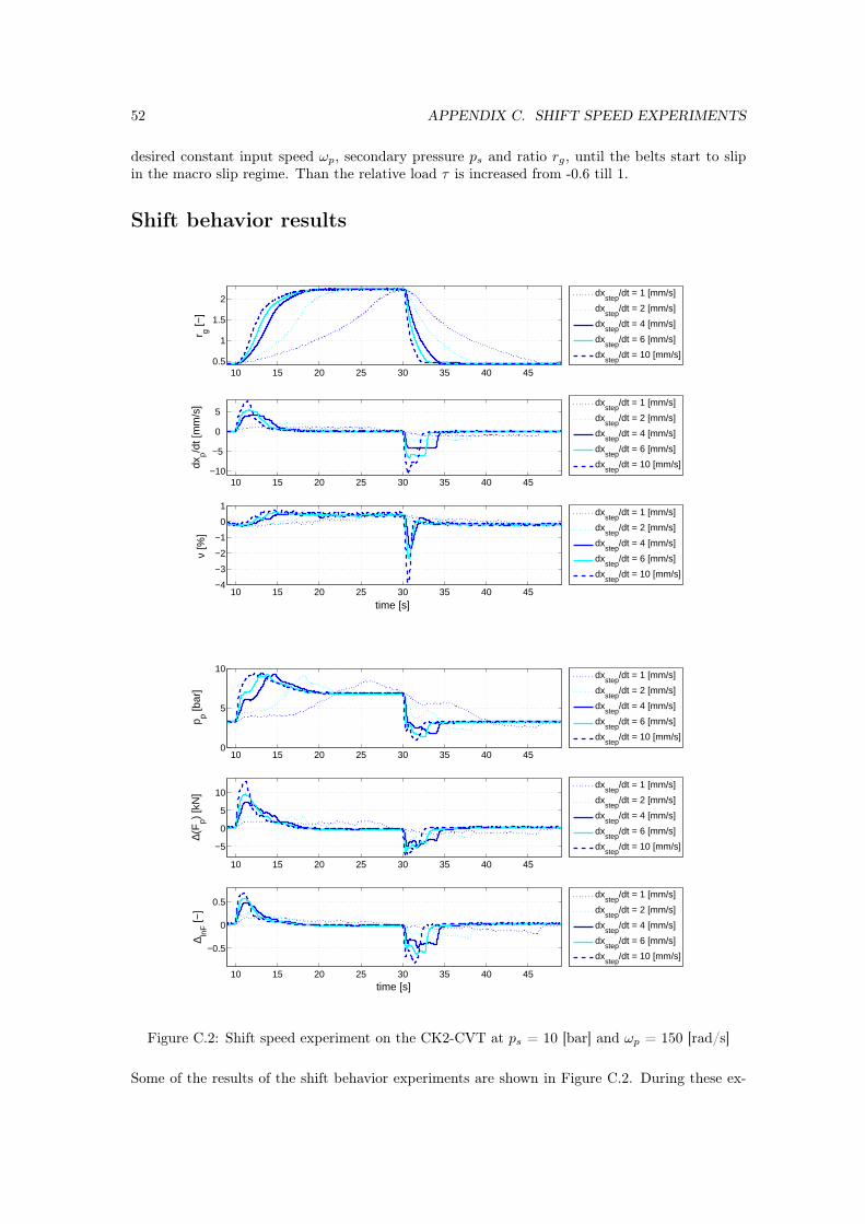
52 APPENDIX C. SHIFT SPEED EXPERIMENTS
desired constant input speed ωp, secondary pressure ps and ratio rg, until the belts start to slipin the macro slip regime. Than the relative load τ is increased from -0.6 till 1.
Shift behavior results
10 15 20 25 30 35 40 450.5
1
1.5
2
r g [−]
dx
step/dt = 1 [mm/s]
dxstep
/dt = 2 [mm/s]
dxstep
/dt = 4 [mm/s]
dxstep
/dt = 6 [mm/s]
dxstep
/dt = 10 [mm/s]
10 15 20 25 30 35 40 45−10
−5
0
5
dxp/d
t [m
m/s
]
dxstep
/dt = 1 [mm/s]
dxstep
/dt = 2 [mm/s]
dxstep
/dt = 4 [mm/s]
dxstep
/dt = 6 [mm/s]
dxstep
/dt = 10 [mm/s]
10 15 20 25 30 35 40 45−4
−3
−2
−1
0
1
ν [%
]
time [s]
dx
step/dt = 1 [mm/s]
dxstep
/dt = 2 [mm/s]
dxstep
/dt = 4 [mm/s]
dxstep
/dt = 6 [mm/s]
dxstep
/dt = 10 [mm/s]
10 15 20 25 30 35 40 450
5
10
p p [bar
]
dx
step/dt = 1 [mm/s]
dxstep
/dt = 2 [mm/s]
dxstep
/dt = 4 [mm/s]
dxstep
/dt = 6 [mm/s]
dxstep
/dt = 10 [mm/s]
10 15 20 25 30 35 40 45
−5
0
5
10
∆(F
p) [k
N]
dx
step/dt = 1 [mm/s]
dxstep
/dt = 2 [mm/s]
dxstep
/dt = 4 [mm/s]
dxstep
/dt = 6 [mm/s]
dxstep
/dt = 10 [mm/s]
10 15 20 25 30 35 40 45
−0.5
0
0.5
∆ lnF [−
]
time [s]
dx
step/dt = 1 [mm/s]
dxstep
/dt = 2 [mm/s]
dxstep
/dt = 4 [mm/s]
dxstep
/dt = 6 [mm/s]
dxstep
/dt = 10 [mm/s]
Figure C.2: Shift speed experiment on the CK2-CVT at ps = 10 [bar] and ωp = 150 [rad/s]
Some of the results of the shift behavior experiments are shown in Figure C.2. During these ex-

53
periments, CVT ratio rg is changed from lowdrive to overdrive and back. By controlling the speedof the stepper motor, different levels of shifting speed are achieved. These experiments are alsocarried out at higher secondary pressure ps, different input speeds ωp and higher stepper motorspeeds xstep, but the results shown are the most representable for shifting while using slip control.
At this pressure level (ps = 10 [bar]), shifting speeds are bounded due to the limited shiftingforce. Axial primary pulley speed xp is equal to the stepping motor speed xstep till 4 [mm/s]during upshifting and till 6 [mm/s] during downshifting. Also more symmetry between up- anddownshifting regarding shifting force is visible, when denoting it as a logarithmic relation insteadof a linear relation. Slip in tangential direction is hardly influenced by shifting at these operationpoints.

54 APPENDIX C. SHIFT SPEED EXPERIMENTS
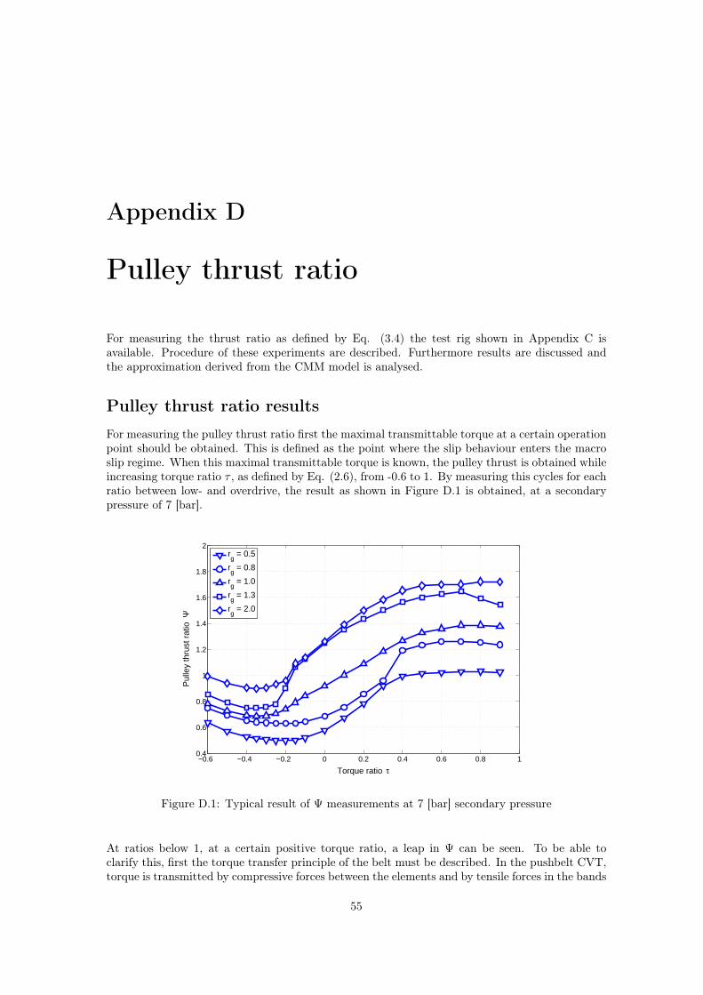
Appendix D
Pulley thrust ratio
For measuring the thrust ratio as defined by Eq. (3.4) the test rig shown in Appendix C isavailable. Procedure of these experiments are described. Furthermore results are discussed andthe approximation derived from the CMM model is analysed.
Pulley thrust ratio results
For measuring the pulley thrust ratio first the maximal transmittable torque at a certain operationpoint should be obtained. This is defined as the point where the slip behaviour enters the macroslip regime. When this maximal transmittable torque is known, the pulley thrust is obtained whileincreasing torque ratio τ , as defined by Eq. (2.6), from -0.6 to 1. By measuring this cycles for eachratio between low- and overdrive, the result as shown in Figure D.1 is obtained, at a secondarypressure of 7 [bar].
−0.6 −0.4 −0.2 0 0.2 0.4 0.6 0.8 10.4
0.6
0.8
1
1.2
1.4
1.6
1.8
2
Torque ratio τ
Pul
ley
thru
st r
atio
Ψ
rg = 0.5
rg = 0.8
rg = 1.0
rg = 1.3
rg = 2.0
Figure D.1: Typical result of Ψ measurements at 7 [bar] secondary pressure
At ratios below 1, at a certain positive torque ratio, a leap in Ψ can be seen. To be able toclarify this, first the torque transfer principle of the belt must be described. In the pushbelt CVT,torque is transmitted by compressive forces between the elements and by tensile forces in the bands
55
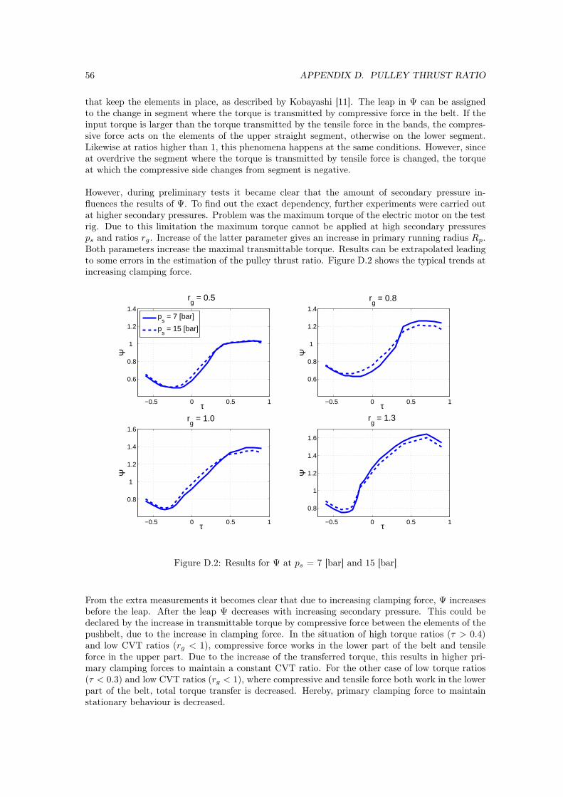
56 APPENDIX D. PULLEY THRUST RATIO
that keep the elements in place, as described by Kobayashi [11]. The leap in Ψ can be assignedto the change in segment where the torque is transmitted by compressive force in the belt. If theinput torque is larger than the torque transmitted by the tensile force in the bands, the compres-sive force acts on the elements of the upper straight segment, otherwise on the lower segment.Likewise at ratios higher than 1, this phenomena happens at the same conditions. However, sinceat overdrive the segment where the torque is transmitted by tensile force is changed, the torqueat which the compressive side changes from segment is negative.
However, during preliminary tests it became clear that the amount of secondary pressure in-fluences the results of Ψ. To find out the exact dependency, further experiments were carried outat higher secondary pressures. Problem was the maximum torque of the electric motor on the testrig. Due to this limitation the maximum torque cannot be applied at high secondary pressuresps and ratios rg. Increase of the latter parameter gives an increase in primary running radius Rp.Both parameters increase the maximal transmittable torque. Results can be extrapolated leadingto some errors in the estimation of the pulley thrust ratio. Figure D.2 shows the typical trends atincreasing clamping force.
−0.5 0 0.5 1
0.6
0.8
1
1.2
1.4
rg = 0.5
τ
Ψ
−0.5 0 0.5 1
0.6
0.8
1
1.2
1.4
rg = 0.8
τ
Ψ
−0.5 0 0.5 1
0.8
1
1.2
1.4
1.6
rg = 1.0
τ
Ψ
−0.5 0 0.5 1
0.8
1
1.2
1.4
1.6
rg = 1.3
τ
Ψ
ps = 7 [bar]
ps = 15 [bar]
Figure D.2: Results for Ψ at ps = 7 [bar] and 15 [bar]
From the extra measurements it becomes clear that due to increasing clamping force, Ψ increasesbefore the leap. After the leap Ψ decreases with increasing secondary pressure. This could bedeclared by the increase in transmittable torque by compressive force between the elements of thepushbelt, due to the increase in clamping force. In the situation of high torque ratios (τ > 0.4)and low CVT ratios (rg < 1), compressive force works in the lower part of the belt and tensileforce in the upper part. Due to the increase of the transferred torque, this results in higher pri-mary clamping forces to maintain a constant CVT ratio. For the other case of low torque ratios(τ < 0.3) and low CVT ratios (rg < 1), where compressive and tensile force both work in the lowerpart of the belt, total torque transfer is decreased. Hereby, primary clamping force to maintainstationary behaviour is decreased.
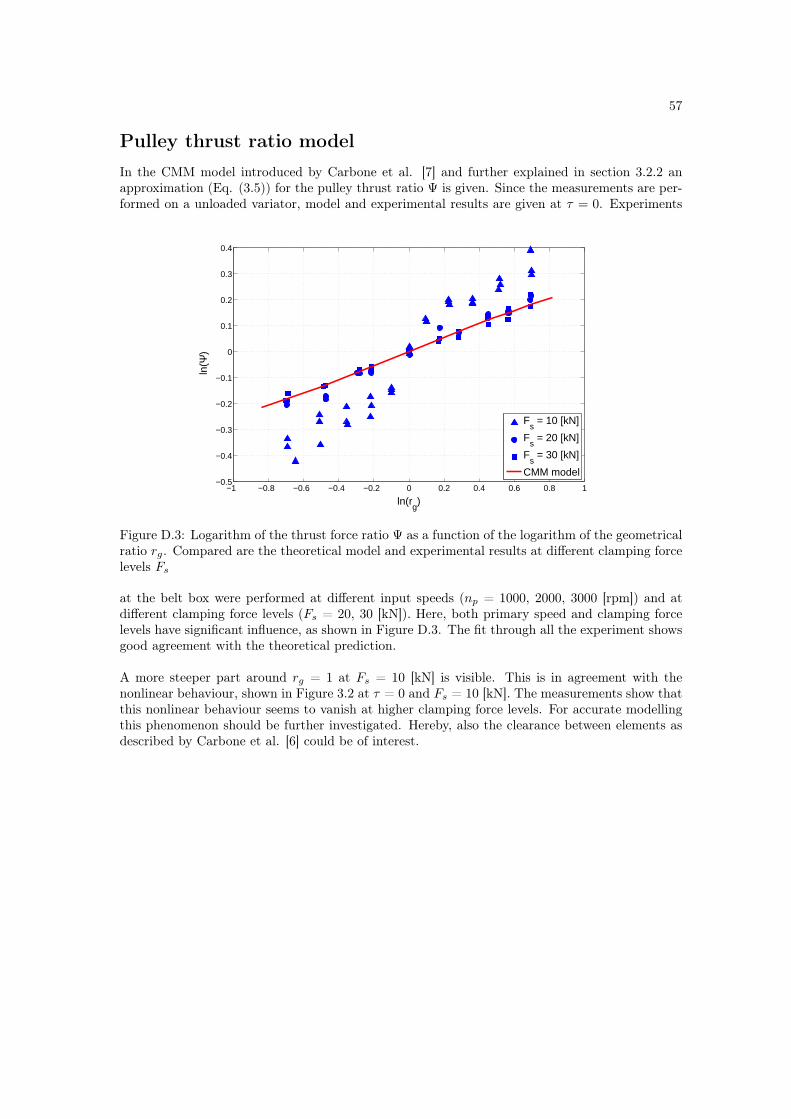
57
Pulley thrust ratio modelIn the CMM model introduced by Carbone et al. [7] and further explained in section 3.2.2 anapproximation (Eq. (3.5)) for the pulley thrust ratio Ψ is given. Since the measurements are per-formed on a unloaded variator, model and experimental results are given at τ = 0. Experiments
−1 −0.8 −0.6 −0.4 −0.2 0 0.2 0.4 0.6 0.8 1−0.5
−0.4
−0.3
−0.2
−0.1
0
0.1
0.2
0.3
0.4
ln(rg)
ln(Ψ
)
Fs = 10 [kN]
Fs = 20 [kN]
Fs = 30 [kN]
CMM model
Figure D.3: Logarithm of the thrust force ratio Ψ as a function of the logarithm of the geometricalratio rg. Compared are the theoretical model and experimental results at different clamping forcelevels Fs
at the belt box were performed at different input speeds (np = 1000, 2000, 3000 [rpm]) and atdifferent clamping force levels (Fs = 20, 30 [kN]). Here, both primary speed and clamping forcelevels have significant influence, as shown in Figure D.3. The fit through all the experiment showsgood agreement with the theoretical prediction.
A more steeper part around rg = 1 at Fs = 10 [kN] is visible. This is in agreement with thenonlinear behaviour, shown in Figure 3.2 at τ = 0 and Fs = 10 [kN]. The measurements show thatthis nonlinear behaviour seems to vanish at higher clamping force levels. For accurate modellingthis phenomenon should be further investigated. Hereby, also the clearance between elements asdescribed by Carbone et al. [6] could be of interest.

58 APPENDIX D. PULLEY THRUST RATIO
Appendix E
Dimensional analysis
From dimensional analysis it can be seen that the CVT dynamical response will depend notseparately on the clamping forces acting on primary and secondary pulley, but on their ratioFp/Fs. If it is assumed for simplicity that the variator is unloaded, CVT design is fixed, and ratiois equal to 1, than the rate of ratio changing is a function of
rg = f(Fp, Fs, ωp) (E.1)
With the assumptions that ωp is constant and if the dependent parameters are divided by Fs bymeans of dimensional analysis the shift speeds only depends on the ratio Fp/Fs, namely
rg = ωpf(Fp/Fs) (E.2)
Not considering actual distribution along the belt, there is a perfect symmetry and primary andsecondary pulley are physically indistinguishable. This yields to the following result
f(Fp, Fs) = −f(Fs, Fp) (E.3)
Beside this property, when both clamping forces are equal shift speed must be zero, independenton the quantity of this force
f(F, F ) = 0 (E.4)
With the given properties the following relation is proposed by Carbone et al. [6]
ln(
Fp
Fs
)= − ln
(Fs
Fp
)(E.5)
Substituting this last relation into Eq. (E.3) gives
f
(ln
Fp
Fs
)= −f
(− ln
Fs
Fp
)(E.6)
The previous equation is an odd function of ln(Fp/Fs). Thus, the Taylor expansion of f mustcontain only odd terms i.e.
f
(ln
Fp
Fs
)≈ c1 ln
Fp
Fs+ c2
(ln
Fp
Fs
)3
+ c3
(ln
Fp
Fs
)5
+ ... (E.7)
The CMM model satisfies Eq. (E.7) under the given hypothesis of no load and ratio equal to 1.Since Fp/Fs is always near 1 in creep mode, higher order terms can be neglected and a secondorder approximation can be given by
f
(ln
Fp
Fs
)≈ c1 ln
Fp
Fs(E.8)
59

60 APPENDIX E. DIMENSIONAL ANALYSIS
This result is obtained by interpreting some physical consideration in a mathematical form. Con-sidering load conditions, influence of friction forces and different values of ratio, the relation willbecome more complicated. However dependency of the logarithm is expected, when Fs is replacedby F ∗
p obtained by rewriting Eq. (E.1) in the form of Eq. (3.3)
rg = 2ωp∆β1 + cos2 β0
sin(2β0)kc(rg)
[ln(
Fp
Fs
)− ln
(F ∗
p
Fs
)](E.9)
Rewriting will give Eq. (3.3).
Appendix F
CMM model
When the friction coefficient µ at the pulley-belt interface and the geometry of the system isknown, the CVT shifting dynamics in creep may simply be described by
rg = ωp∆β1 + cos2 β
sin 2βkc(rg)
[ln
Fp
Fs− lnΨ(rg, τ, ps)
](F.1)
Here, the bending of the pulley can be described as function of the clamping force, retained byexperiments
∆β = d0 + d1Fs (F.2)
with d0 = 6·10−4 and d1 = 2·10−5. The bending of the pulley is only affected by the clampingforce, as expected due to linear elastic response of the system. Dependence on running radius ofthe belt is negligible due to symmetry of the pulley pair. If the belt runs on a high radius on theone pulley it runs on a low radius on the opposite pulley. The term d0 is equal to the bending dueto the clearance between the pulley and its shaft. For no-load conditions ∆β = 6·10−4, which isin good agreement with some data on guidance clearance of the moveable pulley by Tenberge [22].In the pulley model of Sattler [19] ∆β = 1 · 10−3 is assumed constantly, which is in agreementwith measurements at Fs 20 [kN].
The ratio dependent term is defined as
kc(rg) =Rp
argc(rg) (F.3)
with a defined as the axial pulleys distance and
c(rg) = c0 + c1(ln rg)2 (F.4)
The latter relation is a symmetric relation dependent on the logarithm of the ratio, with c0 = 5and c1 = 1.78. To convert the shifting speed to the axial speed of the primary pulley, only thisratio dependent constant will change. Taking the time derivative of rg = Rp/Rs gives
rg = rgRp
Rp
(1− Rs
Rp
rg
)(F.5)
To determine the term Rs/Rp the length of the belt L can be considered as function of Rp andRs by
L = π(Rp + Rs) + 2(Rp −Rs) arcsin(
Rp −Rs
a
)+ 2√
a2 − (Rp −Rs)2 (F.6)
61
62 APPENDIX F. CMM MODEL
Thus neglecting the belt longitudinal deformation and taking the time derivative of Eq. (F.6), thefollowing relation is obtained
− Rs
Rp
=π − 2 arcsin[Rs −Rp)/a]π + 2 arcsin[(Rs −Rp)/a]
=π − 2 arcsin[Rp(1− rg)/rga]π + 2 arcsin[Rp(1− rg)/rga]
(F.7)
With the relations h(rg) = − Rs
Rpand Rp = xp/(2 tan β) Eq. (F.5) can be rewritten to
xp = rgxp
rg(1 + rgh(rg))(F.8)
With this the relation between the axial primary pulley speed xp and the logarithm of the shiftingforce becomes
xp = ωp∆βkc,x(rg)x2p
[ln
Fp
Fs− lnΨ(rg, τ, ps)
](F.9)
with
kc,x(rg) = − cos2 β + 14a (cos2 β − 1)
c(rg)(1 + rgh(rg))
(F.10)
Appendix G
Linearized model
In Section 4.1 the dynamic model for the slip and ratio dynamics are presented. In Eq. (F.6) it isproven that xp is a function of rg only. For deriving all the relations (G) dependent on the ratiorg to state xp the following relation is necessary.
dG
dxp= G′(rg)
drg
dxp(G.1)
withdrg
dxp=
rg
xp[1 + rgh(rg)] (G.2)
Deriving the relations h(rg) and c(rg) with ρ = (2 tanβ)−1 gives
h′(rg) =4πρxp
(π + 2 arcsin(ρxp(1− rg)/rg))2√
r2g − ρ2x2
p(1− rg)2)
1 + h(rg)1 + rgh(rg)
(G.3)
dh
dxp=
4π(1 + h(rg))ρrg
(π + 2 arcsin(ρxp(1− rg)/rg))2√
r2g − ρ2x2
p(1− rg)2)(G.4)
c′(rg) =2c1 ln rg
rg(G.5)
dc
dxp=
2c1 ln rg
xp[1 + rgh(rg)] (G.6)
Deriving the equation of kc,x(rg) and combining it with the previous equations gives
k′c,x(rg) = − cos2 β + 14a (cos2 β − 1)
c′(rg)[1 + rgh(rg)]− c(rg)(h(rg) + rgh′(rg))
[1 + rgh(rg)]2(G.7)
dkc
dxp= − cos2 β + 1
4a (cos2 β − 1)rgc
′(rg)[1 + rgh(rg)]− rgc(rg)(h(rg) + rgh′(rg))
xp[1 + rgh(rg)](G.8)
For the derivative for the logarithm of the shift force
∆ln F (rg, ν) = lnFp
Fs− lnΨ(rg, ν) (G.9)
lnΨ(rg, ν) = m1 ln(rg) + 2m2k1iν + k2i
cos β+ 4m3
(k1iν + k2i)2
cos2 β(G.10)
d∆ln F
dxp= −m1
xp[1 + rgh(rg)]
∆Fp
∆Fp + FsΨ(G.11)
d∆ln F
dν= −
(2m2k1i
cos β+
8m3k1i(k1iν + k2i)cos2 β
)∆Fp
∆Fp + FsΨ(G.12)
63

64 APPENDIX G. LINEARIZED MODEL
Appendix H
Electro-hydraulic system
Figure H.1: Schematic overview of the electro-hydraulic system
65

66 APPENDIX H. ELECTRO-HYDRAULIC SYSTEM
Appendix I
Linearizing shift valve model
As shown in Figure 4.7 this dynamic model is based on the primary pulley pressure pp,val. The in-puts of the model are the controllable input of the stepper motor ustep, the secondary pressure ps,pulley position xp and the axial speed of this pulley xp, which is determined with the CMM model.
Defining the state space as xppv = [pp,val] and uppv =[
ustep xp xp ps
]T the system canbe linearized around a certain working point xppv = [pp,val0] resulting in the linear system
˙xppv = Appvxppv + Bppvuppv (I.1)
where xppv = xppv − xppv,0 and uppv = uppv − uppv,0. With assuming that pd pp0 the linearizedmatrices Appv and Bppv can be derived
Appv = 1σ
[− cf Av0√
2ρoil(ps0−pp0)− cf Apl√
2ρoilpp0
]and
Bppv = 1σ
12Kstepcfkvi1
√2(ps0−pp0)
ρoil
− 12cfkvi1
√2(ps0−pp0)
ρoil− Apkoil
σ
(cfAv0
√2(ps0−pp0)
ρoil− cfApl
√2pp0ρoil
−Apxp0
)−Apcf Av0√
2ρoil(ps0−pp0)
T
for xv0 > 0
While
Appv = 1σ
[cf (Av0−Apl)√
2ρoilpp0
]and
Bppv = 1σ
12Kstepcfkvi1
√2pp0ρoil
− 12cfkvi1
√2pp0ρoil
− Apkoil
σ
(cfAv0
√2pp0ρoil
− cfApl
√2pp0ρoil
−Apxp0
)−Ap
0
T
for xv0 ≤ 0
with
σ = koil(Ap[xp − xp,min] + V0) (I.2)
67
68 APPENDIX I. LINEARIZING SHIFT VALVE MODEL
In this model the position of the spindle attached to the stepper motor is defined by
xstep = Kstepustep (I.3)
It is assumed the dynamics of the stepper motor are much faster compared to the dynamics of thehydraulic valve. Therefore, the output of the stepper motor is proportional with its input with nosignificant delay. Here Kstep has a value of 1.05 · 10−3 [m] per step.
When using the CMM model is used the static gain transfer function H∆ ln F must also be linearizedresulting in the following three relations.
∆ln F
pp,val=
Ap
Appp,val0 − fcpω2p0 + Fs0Ψ0
(I.4)
∆ln F
xp=
m1
xp0[1 + rg0h]
(Appp,val0
Appp,val0 − fcpω2p0 + Fs0Ψ0
)(I.5)
∆ln F
ps=
As
Fs0
(Appp,val0
Appp,val0 − fcpω2p0 + Fs0Ψ0
)(I.6)
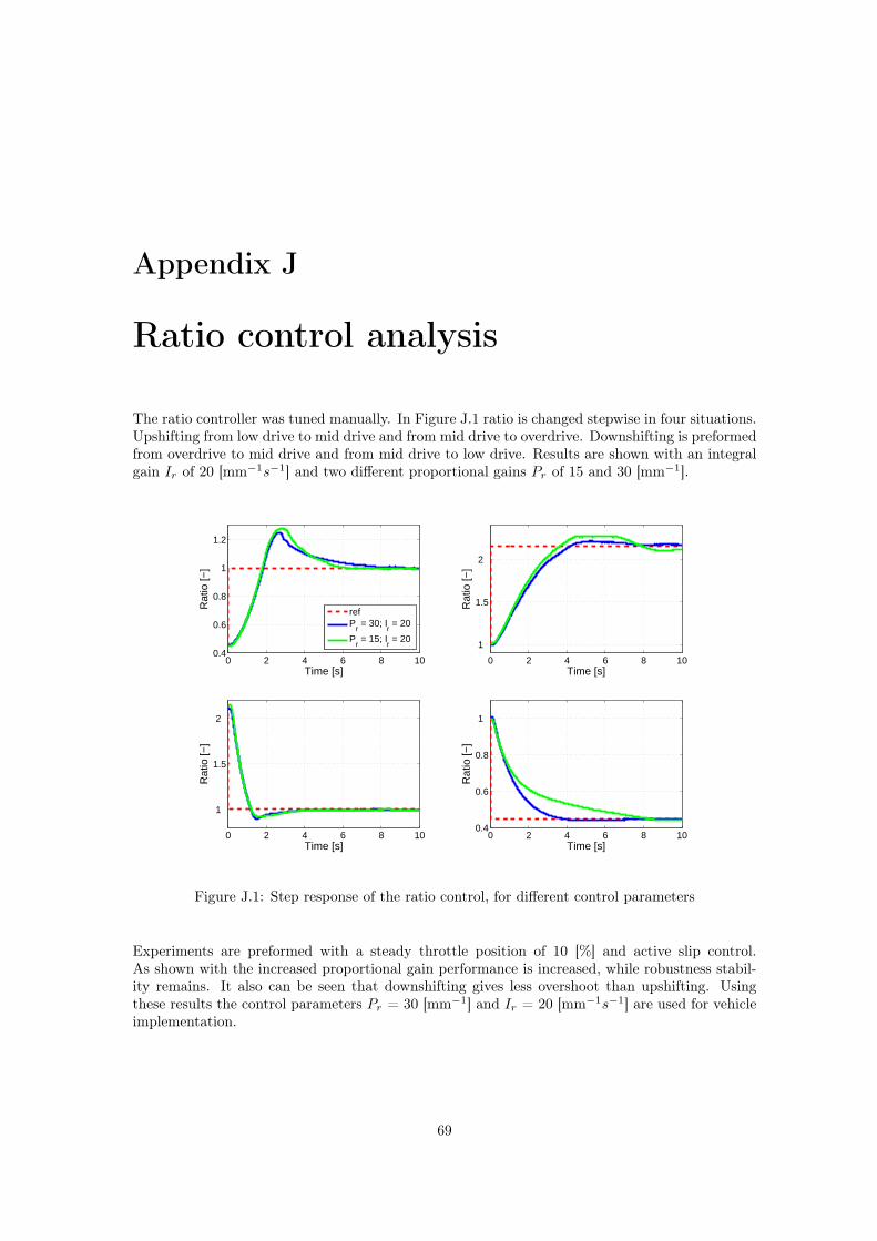
Appendix J
Ratio control analysis
The ratio controller was tuned manually. In Figure J.1 ratio is changed stepwise in four situations.Upshifting from low drive to mid drive and from mid drive to overdrive. Downshifting is preformedfrom overdrive to mid drive and from mid drive to low drive. Results are shown with an integralgain Ir of 20 [mm−1s−1] and two different proportional gains Pr of 15 and 30 [mm−1].
0 2 4 6 8 100.4
0.6
0.8
1
1.2
Time [s]
Rat
io [−
]
0 2 4 6 8 10
1
1.5
2
Time [s]
Rat
io [−
]
0 2 4 6 8 10
1
1.5
2
Time [s]
Rat
io [−
]
0 2 4 6 8 100.4
0.6
0.8
1
Time [s]
Rat
io [−
]
refP
r = 30; I
r = 20
Pr = 15; I
r = 20
Figure J.1: Step response of the ratio control, for different control parameters
Experiments are preformed with a steady throttle position of 10 [%] and active slip control.As shown with the increased proportional gain performance is increased, while robustness stabil-ity remains. It also can be seen that downshifting gives less overshoot than upshifting. Usingthese results the control parameters Pr = 30 [mm−1] and Ir = 20 [mm−1s−1] are used for vehicleimplementation.
69

70 APPENDIX J. RATIO CONTROL ANALYSIS
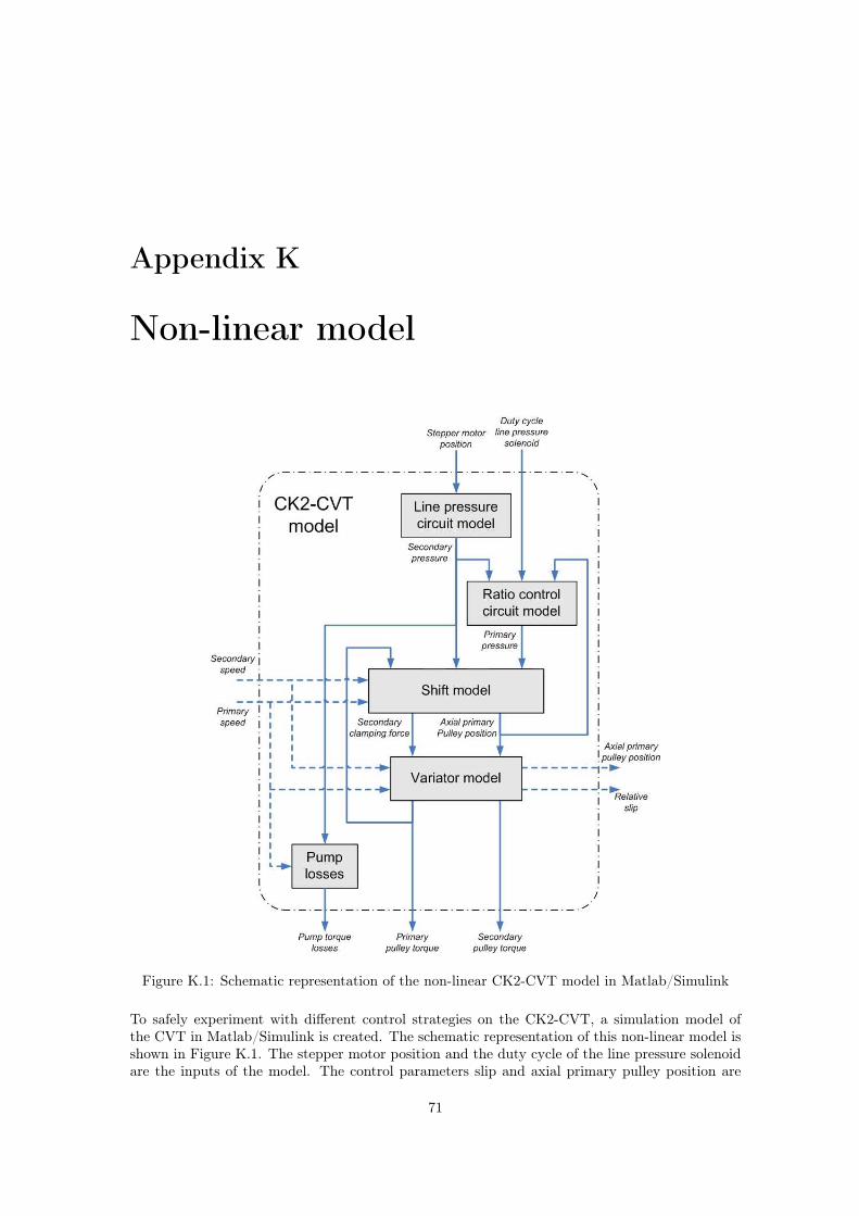
Appendix K
Non-linear model
Figure K.1: Schematic representation of the non-linear CK2-CVT model in Matlab/Simulink
To safely experiment with different control strategies on the CK2-CVT, a simulation model ofthe CVT in Matlab/Simulink is created. The schematic representation of this non-linear model isshown in Figure K.1. The stepper motor position and the duty cycle of the line pressure solenoidare the inputs of the model. The control parameters slip and axial primary pulley position are
71
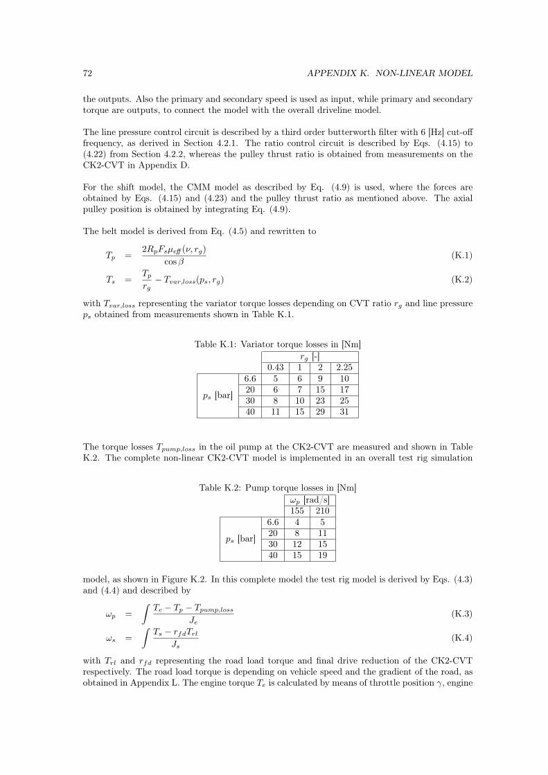
72 APPENDIX K. NON-LINEAR MODEL
the outputs. Also the primary and secondary speed is used as input, while primary and secondarytorque are outputs, to connect the model with the overall driveline model.
The line pressure control circuit is described by a third order butterworth filter with 6 [Hz] cut-offfrequency, as derived in Section 4.2.1. The ratio control circuit is described by Eqs. (4.15) to(4.22) from Section 4.2.2, whereas the pulley thrust ratio is obtained from measurements on theCK2-CVT in Appendix D.
For the shift model, the CMM model as described by Eq. (4.9) is used, where the forces areobtained by Eqs. (4.15) and (4.23) and the pulley thrust ratio as mentioned above. The axialpulley position is obtained by integrating Eq. (4.9).
The belt model is derived from Eq. (4.5) and rewritten to
Tp =2RpFsµeff (ν, rg)
cos β(K.1)
Ts =Tp
rg− Tvar,loss(ps, rg) (K.2)
with Tvar,loss representing the variator torque losses depending on CVT ratio rg and line pressureps obtained from measurements shown in Table K.1.
Table K.1: Variator torque losses in [Nm]rg [-]
0.43 1 2 2.25
ps [bar]
6.6 5 6 9 1020 6 7 15 1730 8 10 23 2540 11 15 29 31
The torque losses Tpump,loss in the oil pump at the CK2-CVT are measured and shown in TableK.2. The complete non-linear CK2-CVT model is implemented in an overall test rig simulation
Table K.2: Pump torque losses in [Nm]ωp [rad/s]155 210
ps [bar]
6.6 4 520 8 1130 12 1540 15 19
model, as shown in Figure K.2. In this complete model the test rig model is derived by Eqs. (4.3)and (4.4) and described by
ωp =∫
Te − Tp − Tpump,loss
Je(K.3)
ωs =∫
Ts − rfdTrl
Js(K.4)
with Trl and rfd representing the road load torque and final drive reduction of the CK2-CVTrespectively. The road load torque is depending on vehicle speed and the gradient of the road, asobtained in Appendix L. The engine torque Te is calculated by means of throttle position γ, engine
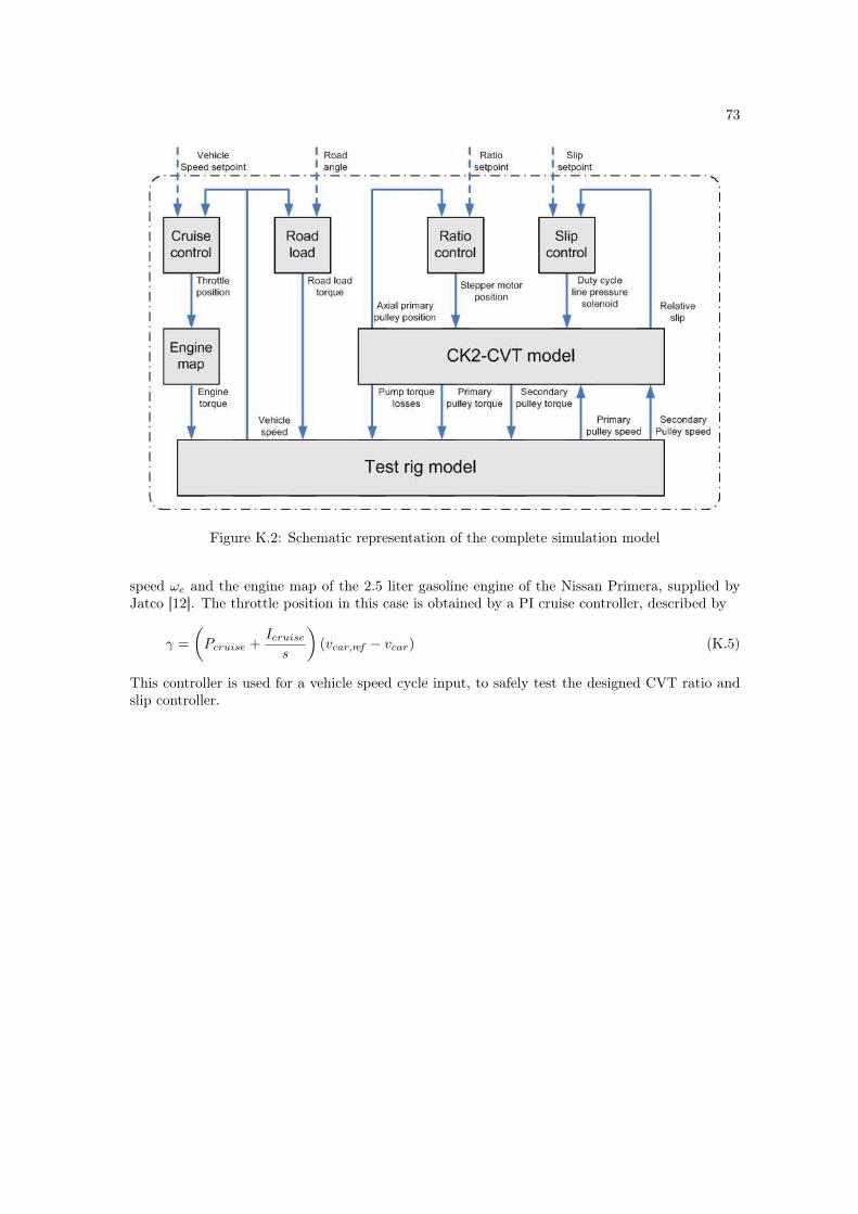
73
Figure K.2: Schematic representation of the complete simulation model
speed ωe and the engine map of the 2.5 liter gasoline engine of the Nissan Primera, supplied byJatco [12]. The throttle position in this case is obtained by a PI cruise controller, described by
γ =(
Pcruise +Icruise
s
)(vcar,ref − vcar) (K.5)
This controller is used for a vehicle speed cycle input, to safely test the designed CVT ratio andslip controller.

74 APPENDIX K. NON-LINEAR MODEL
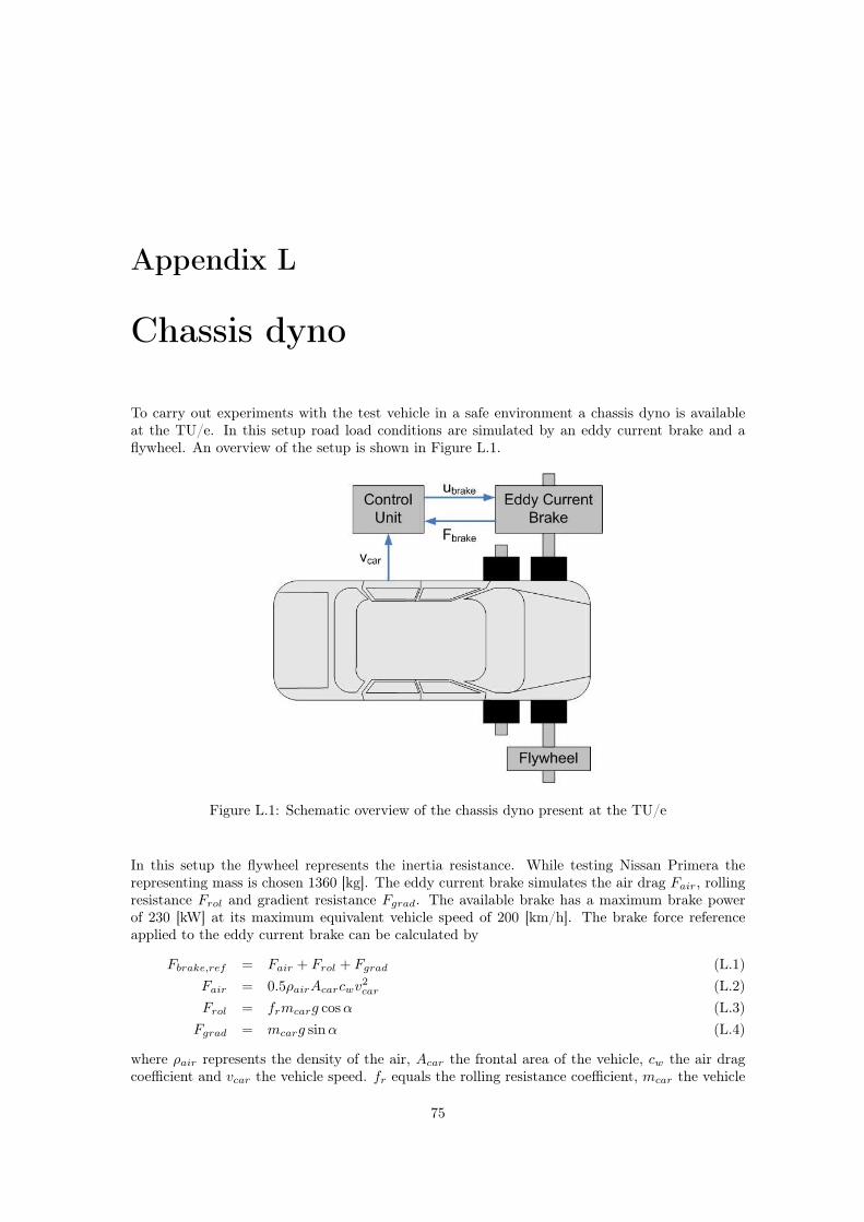
Appendix L
Chassis dyno
To carry out experiments with the test vehicle in a safe environment a chassis dyno is availableat the TU/e. In this setup road load conditions are simulated by an eddy current brake and aflywheel. An overview of the setup is shown in Figure L.1.
Figure L.1: Schematic overview of the chassis dyno present at the TU/e
In this setup the flywheel represents the inertia resistance. While testing Nissan Primera therepresenting mass is chosen 1360 [kg]. The eddy current brake simulates the air drag Fair, rollingresistance Frol and gradient resistance Fgrad. The available brake has a maximum brake powerof 230 [kW] at its maximum equivalent vehicle speed of 200 [km/h]. The brake force referenceapplied to the eddy current brake can be calculated by
Fbrake,ref = Fair + Frol + Fgrad (L.1)Fair = 0.5ρairAcarcwv2
car (L.2)Frol = frmcarg cos α (L.3)
Fgrad = mcarg sinα (L.4)
where ρair represents the density of the air, Acar the frontal area of the vehicle, cw the air dragcoefficient and vcar the vehicle speed. fr equals the rolling resistance coefficient, mcar the vehicle
75
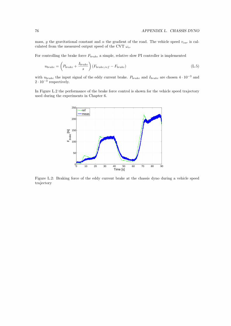
76 APPENDIX L. CHASSIS DYNO
mass, g the gravitational constant and α the gradient of the road. The vehicle speed vcar is cal-culated from the measured output speed of the CVT ωs.
For controlling the brake force Fbrake a simple, relative slow PI controller is implemented
ubrake =(
Pbrake +Ibrake
s
)(Fbrake,ref − Fbrake) (L.5)
with ubrake the input signal of the eddy current brake. Pbrake and Ibrake are chosen 4 · 10−3 and2 · 10−3 respectively.
In Figure L.2 the performance of the brake force control is shown for the vehicle speed trajectoryused during the experiments in Chapter 6.
0 10 20 30 40 50 60 70 80 900
50
100
150
200
250
Time [s]
Fbr
ake [N
]
refmeas
Figure L.2: Braking force of the eddy current brake at the chassis dyno during a vehicle speedtrajectory