Bulletin of the Transilvania University of Braşov • Vol. 9 (58) No. 2 - Special Issue – 2016 Series I: Engineering Sciences

SWERVE CORRECTION OF HEAVY-DUTY

ARTICULATED LORRIES

F. SORGE 1

Abstract: The trailers of heavy-duty articulated lorries are usually linked to the tractors by auxiliary dollies to improve the manoeuvrability along curved paths. Connecting the dolly to the tractor by a four-bar linkage, some performance improvement may be achieved in comparison with the conventional single pin. The correct path along a road curve may be obtained exerting control moments on the horizontal plane by means of differential braking of the wheels. The results of the analysis show that the forward-converging and the crossing bar quadrilaterals are mostly yaw-stable, whereas the backward-converging bars prove to be inherently unstable. Key words: Articulated vehicles, anti-yaw systems.

1 Polytechnic School, University of Palermo, Italy

1. Introduction The transverse conduct of a vehicle

mainly depends on the cornering stiffness of the tyres, which is in turn influenced by the vertical load, the inflation pressure, the cross-section shape and the ply wrapping. Increasing the speed, instability thresholds may be reached even on straight paths and besides, the off-tracking of the long vehicles must be controlled, as the different paths of the first and last axle may involve invasion of the opposite or the emergency lanes.

The vehicle engineers must scrupulously ponder all these aspects, particularly for the long heavy articulated lorries. Electronic stability control systems (ESC) may help in limiting the anomalous steering response [1].They may be of various types: differential braking; steer-by-wire; limited slip differential.

The first theoretical analysis of the vehicle lateral dynamics was perhaps given by Rocard [2]. He stated that the transverse force F exerted by the road on the tyre is roughly proportional to the drift angle εof the wheel and moreover, increases with the vertical load. The treatise of Gillespie reports many experimental results in the chapter on the tyre cornering, highlighting the influence of the inflation pressure, the ply composition and the tyre aspect ratio, [3]. Also, the "magic formula" of Pacejka is worth remembering, as it contains several parameters that may be properly adjusted to fit all types of tyre response [4].

The lateral stability of multi-trailer trucks was examined in the eighties considering several connection arrangements, e. g. by articulated linkages, which often offer interesting stabilizing properties [5]. The promising properties of the four-bar connections motivated

Bulletin of the Transilvania University of Braşov • Series I • Vol. 9 (58) No. 2 Special Issue - 2016 268

previous researches by the author, [6] and [7], and the present analysis, where the self-arising lateral motions along the straight paths are studied and the response to the steering manoeuvres of the driver are quantified. The possible active control of the critical swerve is also considered.

The model is linearized, in the hypothesis of small lateral movements, in order to simplify the study of the influence of the various system characteristics.

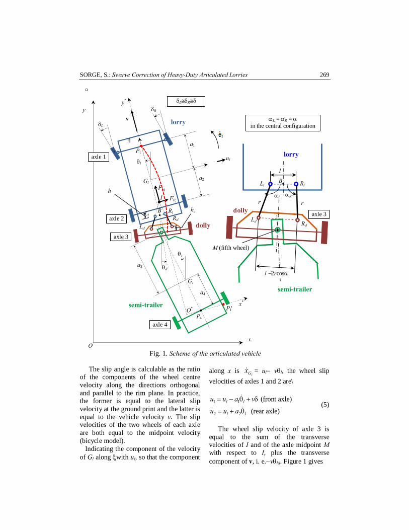
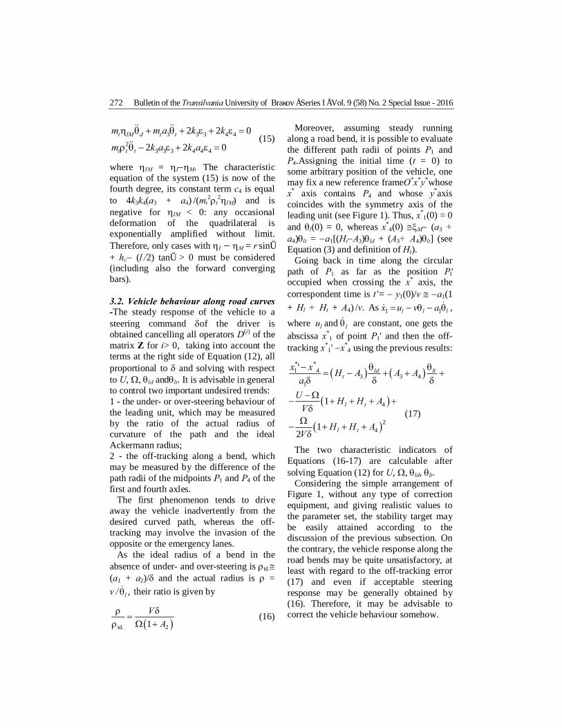
2. Mathematical model 2.1. System geometry - The lorry-dolly-semi-trailer system is schematized in Figure 1, where the dolly is assumed massless and: - the frames Oxy and Glξη are fixed to the

ground and to the leading unit respectively;

- θl, θd and θt are the angles formed by the lorry, the dolly and the trailer with the fixed direction y, whence the relative rotations are θld = θl−θd,θlt = θl−θt;

- Gl and Gt are the centres of mass of the leading and trailing units;

- FIξ and FIη are the components along ξand η of the resultant traction force acting on the dolly through the two connecting bars, which may be applied at the instant centre I of the relative rotation. Notice that the component FIηis approximately the resistant road force acting on the trailer, whence FIη≅ Frolling,t+ Fair,t (where Fair,t = cxρAv2/2);

- δ is the steering angle imposed by the driver, which is assumed of the same small order of magnitude of the yaw rotations and equal for the left and right wheels for simplicity;

- v is the speed of the lorry (|v| = v). Let us define the angles of the left and

right bars, αL = α + ∆αL, αR = α + ∆αR, where α is their common value in the central configuration. Assuming small

transverse displacements, the incremental angles,∆αL and∆αR, and the rotations, θld and θlt, are of the same small order of magnitude, which is also ascribed to the cornering slip angles εof the wheels. Then, imposing proper closure equations to the quadrilateral LlRlRdLd and to the triangle LlIRl like in [7], one gets

12 cosL R ld

lr

∆α ≅ −∆α ≅ − θ α (1)

and derives the linearized coordinatesξ,η of points I and M:

2

1sin 2 2 cos

tan 2

I ld

I

l lr

l a h

ξ ≅ − θ α α α η ≅ − + +

(2)

( )2

tan sin 2

sin

M c ld

M c

l r h

h r a h

α ξ ≅ − α − θ

η ≅ − + α + + (3)

this will be needed in the formulation of the equation of motion. 2.2. Cornering forces and slip angles – The cornering coefficient k=−F/ε depends on many working conditions and several formulas were proposed in the past. For example, some diagrams of [3] show the dependence of k on the vertical load on the tyre (% of rated load) for a typical passenger car. An excellent fit may be obtained by third degree polynomial laws [7].

3

0 0

z z

z z

F F Fk a b cF F

= − = + − ε

(4)

where Fz0 is the rated load and a = 5.092 kN, b = 39.735 kN, c = 6.955 kN. Here, these coefficients will be multiplied by a factor 10, which is roughly the weight ratio of a typical lorry and a saloon car.

SORGE, S.: Swerve Correction of Heavy-Duty Articulated Lorries 269

The slip angle is calculable as the ratio of the components of the wheel centre velocity along the directions orthogonal and parallel to the rim plane. In practice, the former is equal to the lateral slip velocity at the ground print and the latter is equal to the vehicle velocity v. The slip velocities of the two wheels of each axle are both equal to the midpoint velocity (bicycle model).

Indicating the component of the velocity of Gl along ξwith ul, so that the component

along x is lGx& = ul− vθl, the wheel slip

velocities of axles 1 and 2 are\

1 1

2 2

(front axle)

(rear axle) l l

l l

u u a v

u u a

= − θ + δ

= + θ

&

& (5)

The wheel slip velocity of axle 3 is

equal to the sum of the transverse velocities of I and of the axle midpoint M with respect to I, plus the transverse component of v, i. e.−vθld. Figure 1 gives

v

θl

I

y

δR

a1

a2

η

Ll Rl

lorry

FIη

FIξ

ul

h

B

axle 1

axle 2

axle 3

axle 4

semi-trailer

dolly

a3

a4

Ld

Rd

θt

θd

δL

δL≅δR≅δ

x*

P4

Gt

B

lorry

Ll Rl

Ld Rd

l

r r

αL αR

dolly

M (fifth wheel)

O

O*

hc

αL = αR = α in the central configuration

axle 3

P1'

l −2rcosα

G

Gl

P1

y*

semi-trailer

x

Fig. 1. Scheme of the articulated vehicle

Bulletin of the Transilvania University of Braşov • Series I • Vol. 9 (58) No. 2 Special Issue - 2016 270

( )3

(dolly axle)Ml I l I ld du u v= − η θ + η − η θ − θ& &

(6)

Likewise, the wheel slip velocity of axle 4is obtainable summing, to the transverse velocity of M, the velocity of its midpoint with respect to M, plus the component−v(θlt−θld)

( ) ( )3 3 44

(trailer axle)+ + += θ θ − θ&

ld lttu a a vu (7)

Hence, the slip angles areεi = ui /v, and the cornering forces are Fi= −2kiεi for each axle.

2.3. Equations of motion - All sway motions are characterized by four state variables, ul, lθ& , θld, and θlt, but six dynamical equations must be formulated in total for the three units, three translational ones along x and three rotational ones on the horizontal plane. Yet, two equations drop when summing all translational equations to eliminate the mutual transverse forces, FIξ exchanged at I, and FMξ exchanged at M. It is remarkable that the coordinates of Gl and the orientation θl of the leading unit with respect to the fixed frame Oxy are irrelevant, because this frame might be placed in any arbitrary position with any arbitrary orientation.

Thus, we get at last

( )( )l t l l t lIm m u v m+ − θ − η +θ& &&&

( )( )Mt dI l lm θη θη − +− && &&

( )3 ηθ − θ θ ++&& &&t l lt I ltm a F

1 1 2 2 3 3 4 42 2 2 2 0k k k kε + ε + ε + ε = (translation of whole vehicle) (8)

( )2

2 2 2 1 1 1

1 1 2 2

,

2 2

2 2

1sin 2 2 cosη

ρ θ + ε − ε

η − θ + ε + ε + − θ α

+

=α

&&

&&

l l

I

l

I l l

z l

l

ld

m k a k a

m u v k k

l lF mr

(rotation of leading unit) (9)

( ) ( )]2 4 4

23 1 1

4 ,2 3 3 3

2

2 2 2 η

ρ − − − θ + ε +ε + ε + ε =−

θ θ

θ

&& && &&

I z

t t l l l

t t

lt l

l

m a m u v k

k k k a mF a (rotation of trailing unit) (10)

( ) ( ) 1 1 2 2

1sin 2 2 cos

2 2

0η − + η − ηα α

η − η − θ + ε + ε + θ

=

&&

I M

I M l l

ldI

l

l l

r

m u v k k

F

(rotation of dolly) (11) Here ρl and ρt are the radii of gyration of

the tractor and the trailer and mz,l and mz,t indicate the correction moments exerted on the leading and trailing units by some possible correction system.

2.4. Non-dimensional formulation -Introduce the reference cornering stiffness k0 = a+b−c and the reference speed 0 0 1 / lv k a m= , and define dimensionless parameters and variables by capital letters: Ai = ai/a1, Ki = ki /k0, V = v/v0, U = ul /v0,Ω= a1 lθ& /v0, Ρj = ρj/a1, Mz,j= mz,j/(2a1k1δ). Moreover, indicate for brevity: ca = Fair,t /(k0V2),cr = Frolling,t/k0,µ = mt/ml Hl= − ηI /a1 = (a2 + h+ ltanα /2) /a1 Ht= (ηI − ηM + a3)/a1= = (a3 +hc +rsinα−ltanα /2) /a1 L =

11

sin 2 2 cosl l

a r − α α

Also, introduce the dimensionless time variable τ = v0t /a1 and the differential operators

D(i)(...) = di(...) /dτ i = (a1 /v0) idi(...) /dt i

SORGE, S.: Swerve Correction of Heavy-Duty Articulated Lorries 271

The equations of motions (8-11) may be made non-dimensional dividing the translational equation, Equation (8), by k0 and the moment equations, Equations (9-11), by k0a1. Hence, one obtains

,1

3 ,

3

11

2 l z l

ld z t

lt t

UH M

KA MA H

− Ω + + = δ θ + θ −

Z (12)

where the coefficients of the dynamical matrix Z are linear functions of D(0), D(1), D(2), and depend on V. 3. Results

The stability analysis requires the examination of the negative ness of the real part of the eigenvalues of Z. The response of the articulated vehicle to a steering maneuver of the driver is obtainable by solving the complete non- homogeneous system.

3.1. Stability - Replacing the operators D(i)

of Z with the ith powers of the characteristic number λ, we get a sixth degree algebraic equation, whose coefficients ci are functions of the dimensionless vehicle velocity V,

41 2

6 55 6... 0c c c cλ + λ + λ + λ + =+ (13)

The divergent instability threshold is determined equating c6 to zero, whereas the oscillating instability threshold may be obtained putting λ = ± iω and equating the real and imaginary parts of the characteristic equation to zero separately:

( )6 4 2

6

43

2

1 5

4

2

0

0

c c

i

c

c c c

ω − ω + −

+

ω =

± ω ω − ω = (14)

Hence, choosing one significant parameter of the car train, for example the dimensionless distance A4 of the fourth

axle from the trailer mass centre, one has to explore the operative velocity region of the vehicle in search of instability. For each velocity V, it is possible to vary A4 by steps and search the divergent instability threshold, where c6 vanishes. At the same time, it is possible to look for the oscillating instability threshold where, after calculating the two roots ω2 of the second of Equations (14) and checking that either or both of them are real and positive, they are found to satisfy the first equation as well. Mind also that, apart from this search, the stability of any point of the map (A4,V) may be checked by the Hurwitz criterion.

Several connection configurations of the four bar linkage may be analysed this way and stability maps may be traced. The range of A4must not be too large for a well-balanced load distribution on the axles, whereas the range of V = v/v0 is here chosen between 0 and 5, which is consistent somehow with the lorry operation, as the usual values of k0, a1 and ml give v0≅3-4 m/s (10-15 km/h). The other parameters of the articulated vehicle may be held fixed.

The results indicate in general that the configurations with forward converging side bars show wide region of stability in their operating range. On the contrary, the backward converging bars may be stable if they intersect before point M, but always lead to divergent instability if they intersect behind M, independently of the vehicle speed, due to a real positive eigenvalue. This is an intrinsic instability of the latter trailer connection. Actually, neglecting the resistance FIη and looking for natural modes that do not involve the tractor (ul= θl = 0), Equations (9,11) would be identically satisfied, whereas Equations (8,10) would reduce to

Bulletin of the Transilvania University of Braşov • Series I • Vol. 9 (58) No. 2 Special Issue - 2016 272

4 43 3 3

4 43 42

3 3

2 2 0

2 2 0

θ + θ + ε + ε =η

=ρ − εθ ε +

&& &

&&

&t tIM d t

t t t

m m a k k

m k a k a (15)

where ηIM = ηI−ηM. The characteristic equation of the system (15) is now of the fourth degree, its constant term c4 is equal to 4k3k4(a3 + a4) /(mt

2ρt2ηIM) and is

negative for ηIM < 0: any occasional deformation of the quadrilateral is exponentially amplified without limit. Therefore, only cases with ηI − ηM = r sinα + hc− (l /2) tanα > 0 must be considered (including also the forward converging bars). 3.2. Vehicle behaviour along road curves -The steady response of the vehicle to a steering command δof the driver is obtained cancelling all operators D(i) of the matrix Z for i> 0, taking into account the terms at the right side of Equation (12), all proportional to δ and solving with respect to U, Ω, θld andθlt. It is advisable in general to control two important undesired trends: 1 - the under- or over-steering behaviour of the leading unit, which may be measured by the ratio of the actual radius of curvature of the path and the ideal Ackermann radius; 2 - the off-tracking along a bend, which may be measured by the difference of the path radii of the midpoints P1 and P4 of the first and fourth axles.

The first phenomenon tends to drive away the vehicle inadvertently from the desired curved path, whereas the off-tracking may involve the invasion of the opposite or the emergency lanes.

As the ideal radius of a bend in the absence of under- and over-steering is ρid.≅ (a1 + a2)/δ and the actual radius is ρ = v / ,lθ& their ratio is given by

( )id. 21V

Aρ δ=

ρ Ω + (16)

Moreover, assuming steady running along a road bend, it is possible to evaluate the different path radii of points P1 and P4.Assigning the initial time (t = 0) to some arbitrary position of the vehicle, one may fix a new reference frameO*x*y*whose x* axis contains P4 and whose y*axis coincides with the symmetry axis of the leading unit (see Figure 1). Thus, x*

1(0) = 0 and θl(0) = 0, whereas x*

4(0) ≅ξM− (a3 + a4)θlt = −a1[(Ht−A3)θld + (A3+ A4)θlt] (see Equation (3) and definition of Ht).

Going back in time along the circular path of P1 as far as the position P1' occupied when crossing the x* axis, the correspondent time is t '= − y1(0)/v ≅ −a1(1 + Hl + Ht + A4) /v. As 1 1 l l lx u v a= − θ − θ&& ,

where and l lu θ& are constant, one gets the abscissa x*

1 of point P1' and then the off-tracking x*

1' −x*4 using the previous results:

( ) ( )* *1

31

43 4

' ld ltt

x A Ax H Aa− θ θ

= + +δ δ

− +δ

( )

( )

4

42

1

12

l t

l t

U H H AV

H H AV

− Ω− + + + +

+ + +δ

Ωδ

− (17)

The two characteristic indicators of Equations (16-17) are calculable after solving Equation (12) for U, Ω, θld, θlt.

Considering the simple arrangement of Figure 1, without any type of correction equipment, and giving realistic values to the parameter set, the stability target may be easily attained according to the discussion of the previous subsection. On the contrary, the vehicle response along the road bends may be quite unsatisfactory, at least with regard to the off-tracking error (17) and even if acceptable steering response may be generally obtained by (16). Therefore, it may be advisable to correct the vehicle behaviour somehow.

SORGE, S.: Swerve Correction of Heavy-Duty Articulated Lorries 273

∗′−∗

Using sophisticated electronic systems, which detect the anomalous trend of the vehicle run through the signals coming from accelerometers or gyroscopic sensors, it is possible to apply anti-yaw correction moments on the two units, by use of differential braking systems or availing of limited slip differential. Nonetheless, much simpler devices are also conceivable, which apply the correction moments in a constant way, independently of the vehicle speed, but proportionally to the steering angle δ. This type of correction might be easily realized by simple hydraulic or pneumatic devices, which exploit possible installations already existing on board and supply an output proportional to δ for the differential braking.

Due to the linearity of Equation (12), the steady displacement solution vector, d = U, Ω, θld, θltT may be expressed in the form

0,0 , 1,0 , 0,1z l z tM M= + +d d d d (18)

where the subscripts i,j of di,j indicate the values imposed to Mz,l and Mz,t, respectively, when solving Equation (12) for d. Of course, the vectors di,j are functions of the speed V, whence one

obtains, by Equations (16-17),

( ) ( ) ( )0 ,id.

,1 l z l t z tV b V Mb b V Mρ− + +=

ρ

( ) ( ) ( )* *1

0 , ,1

4'l z l t z t

x x c V c V M c V Ma−

= + +δ

(19)

An excellent correction of the vehicle response along the bends may be obtained by imposing opposite values to each of the two indicators, ρ/ρid.− 1 and (x*

1' −x*

4)/(a1δ), for V = 0 and V = Vx, where Vx is a properly chosen upper limit of response acceptableness, e. g. Vx = 4. This constraints permit to write

( ) ( ) ( ) ( )( ) ( )

( ) ( ) ( ) ( )( ) ( )

, ,

0 0

, ,

0 0

0 0

0

0 0

0

l l x z l t t x z t

x

l l x z l t t x z t

x

b b V M b b V M

b b V

c c V M c c V M

c c V

+ + + = − +

+ + + = − +

(20)

and solve for the desired moments, Mz,l and Mz,t, which are independent of the speed V. According to the previous definition of the non-dimensional moments Mz, the true physical moments mz are proportional to δ,

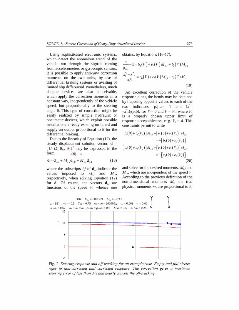
Fig. 2. Steering response and off-tracking for an example case. Empty and full circles refer to non-corrected and corrected response. The correction gives a maximum steering error of less than 3% and nearly cancels the off-tracking.

Data: Mz,l = −0.0359 Mz,t = −2.33 α = 92° r/a1 = 0.5 l/a1 = 0.75 ml = mt= 20000 kg ca = 0.001 cr = 0.02 a2/a1 = 0.67 a3 = a4 = a1 ρl /a1 = ρt /a1 = 0.6 h/ a1 = 0.5 hc / a1 = 0.25

.

15

10

5

0

-5

Bulletin of the Transilvania University of Braşov • Series I • Vol. 9 (58) No. 2 Special Issue - 2016 274

which is then the only quantity ruling the anti-yaw control.

Figure 3 reports the results for an example case, where the side bars are slightly diverging backward. It is observable that the correction aid, as described above, is very beneficial in nearly cancelling the path errors, especially with regard to the off-tracking. The correction moment Mz,l is just small, but its implementation is convenient all the same, as some significant over-steering would appear without it.

4. Conclusion

The four bar linkage may offer a good connection configuration of the tractor-dolly-trailer systems for heavy duty operation, provided that the side bars diverge backward, or their convergence point is at least ahead of the trailer coupling point, in order to preserve the lateral stability en route.

A good correction of the undesired motions along the road bends may be achieved by applying differential braking to the wheels, to produce proper anti-

swerve moments, which are independent of the speed and proportional to the steering angle.

References 1. Rajamani, R.: 2006 Vehicle Dynamic

and Control. Springer, 2006. 2. Rocard, Y.: L'instabilité en

Mécanique.Paris. Masson et C., 1954. 3. Gillespie, T.D.: Fundamental of Vehicle

Dynamics. SAE International, 1992. 4. Pacejka, H.B.: Tyre and Vehicle

Dynamics. Oxford. Butterworths, 2006. 5. Winkler, C.B.: Innovative Dollies:

Improving the Dynamic Performances of Multi-Trailer Vehicles. In:Weights and Dimens., Kelowna, Canada. 1986.

6. Sorge, F.: On the Sway Stability Improvement of Car-Caravan Systems by Articulated Connections.In: Vehicle System Dynamics.Vol. 53-9, p. 1349-1372.

7. Sorge, F.: Optimization of Vehicle-Trailer Connection Systems. In: MoViC-RASD 2016, Southampton, UK,2016