Embed Size (px)
Citation preview

IZA DP No. 2314
Swedish Labor Market Trainingand the Duration of Unemployment
Katarina RichardsonGerard J. van den Berg
DI
SC
US
SI
ON
PA
PE
R S
ER
IE
S
Forschungsinstitutzur Zukunft der ArbeitInstitute for the Studyof Labor
September 2006
Swedish Labor Market Training
and the Duration of Unemployment
Katarina Richardson IFAU Uppsala
Gerard J. van den Berg
Free University Amsterdam, Princeton University, IFAU Uppsala, IFS, CEPR and IZA Bonn
Discussion Paper No. 2314 September 2006
IZA
P.O. Box 7240 53072 Bonn
Germany
Phone: +49-228-3894-0 Fax: +49-228-3894-180
Email: [email protected]
Any opinions expressed here are those of the author(s) and not those of the institute. Research disseminated by IZA may include views on policy, but the institute itself takes no institutional policy positions. The Institute for the Study of Labor (IZA) in Bonn is a local and virtual international research center and a place of communication between science, politics and business. IZA is an independent nonprofit company supported by Deutsche Post World Net. The center is associated with the University of Bonn and offers a stimulating research environment through its research networks, research support, and visitors and doctoral programs. IZA engages in (i) original and internationally competitive research in all fields of labor economics, (ii) development of policy concepts, and (iii) dissemination of research results and concepts to the interested public. IZA Discussion Papers often represent preliminary work and are circulated to encourage discussion. Citation of such a paper should account for its provisional character. A revised version may be available directly from the author.
IZA Discussion Paper No. 2314 September 2006
ABSTRACT
Swedish Labor Market Training and the Duration of Unemployment*
The vocational employment training program is the most ambitious and expensive training program in Sweden and a cornerstone of labor market policy. We analyze causal effects on the individual transition rate from unemployment to employment by exploiting variation in the timing of treatment and outcome, dealing with selectivity on unobservables. We demonstrate the appropriateness of this approach in our context by studying the assignment. We also develop a model allowing for duration dependence and unobserved heterogeneity (leading to spurious duration dependence) in the treatment effect, and we prove non-parametric identification. The data cover the population and include multiple unemployment spells for many individuals. The results indicate a large significantly positive effect on exit to work shortly after exiting the program. The effect at the individual level diminishes after some weeks. When taking account of the time spent in the program, the effect on the mean unemployment duration is often close to zero. JEL Classification: J64, C14 Keywords: vocational training, program evaluation, duration analysis, selectivity bias,
treatment effect, duration dependence, identification Corresponding author: Katarina Richardson IFAU Uppsala Box 513 75120 Uppsala Sweden E-Mail: [email protected]
* We thank the Swedish National Labour Market Board (AMS) and Statistics Sweden (SCB) for their permission to use the data. We thank Richard Smith, Annette Bergemann, Håkan Regnér, Anders Harkman, and other participants in conferences in Stockholm, Uppsala, and Rotterdam, and seminars at Aarhus, Bristol, Mannheim, UCL London, Humboldt, Oxford, and LSE, as well as our colleagues at IFAU, for helpful comments. In addition, we thank Helge Bennmarker for help with the data.
1 Introduction
Training programs for the unemployed have been cornerstones of labor market policy for
many decades. In Sweden, training programs have been used since 1918 and constitute an
important part of the so-called Swedish model (or Nordic model) of labor market policy.
Among Sweden’s current programs, the employment training program (which we denote
by its Swedish acronym AMU) is the most prestigious. AMU aims to improve the chances
of unemployed job seekers to obtain a job, by way of substantive skill-enhancing courses.
In 1997, on average 37,000 individuals were participating in AMU per month, which cor-
responds to over 10% of total unemployment.1 AMU is the most expensive active labor
market program in Sweden and as such it adds to the tax burden. Nevertheless, the number
of evaluation studies is rather small, and most of these analyze the effect of AMU on the
participants’ annual earnings and/or use data from early eighties and/or data on special
subgroups of unemployed workers, notably youths in Stockholm (see references below).
This paper provides a comprehensive empirical analysis of the effect of AMU on the in-
dividual transition rate from unemployment to employment. Note that the officially stated
objective of AMU is to generate a positive effect. The results are of obvious importance for
the evaluation of the AMU program and the underlying “Swedish model”. In addition, they
are of importance in the light of the recent policy shifts in many other countries towards
an increased use of active measures of bringing the unemployed back to work, notably by
way of reschooling unemployed workers with low skills or obsolete qualifications (see e.g.
Fay, 1996).
We use matched longitudinal register data of the full population of individuals who
were unemployed in Sweden within the period from January 1, 1993 until June 22, 2000.
The data include detailed records from employment offices, records from unemployment
insurance agencies, and income tax records. The employment office data report the exact
types of training and the corresponding dates of entry and exit.
The empirical analysis applies a methodology in which the information in the timing
of events (like the moment at which the individual enrols in training and the moment at
which he finds a job) is used to estimate causal treatment effects in the presence of “selec-
tivity on unobservables”. This Timing of Events approach involves estimation of models
that simultaneously explain the duration until an outcome of interest and treatment sta-
tus. The treatment is allowed to affect the main outcome by way of the time rate at which
the latter occurs after the treatment. Abbring and Van den Berg (2003) provided a for-
mal underpinning of the approach by proving non-parametric identification in a number
of settings.2 In addition, they provide a systematic account of the behavioral assumptions
1In 2000, these figures are 30,000 and 9%, respectively (see AMU, 2001).2A major advantage of the approach is that it does not require exclusion restrictions on the set of
1
that are required for a valid use of this approach. Notably, individuals are not allowed to
anticipate the moment at which the treatment occurs, although they are allowed to know
the distribution of this moment over time. Many of the requirements for the use of this
approach also apply to other treatment evaluation methods, including those that do not
focus on dynamic treatment assignment or on a duration variable as main outcome. Nev-
ertheless, they are often neglected in the empirical literature, including empirical studies
of treatment effects on duration variables. We explain in detail that AMU fits well into
the methodological framework, contrary to other labor market training programs and ac-
tive labor market programs in Sweden. To substantiate our claims we use evidence from
discussions with caseworkers, and we also rely on existing studies on unemployment, unem-
ployment insurance, and active labor market programs in Sweden. These include Eriksson
(1997a, 1997b), Zettermark et al. (2000), Carling and Richardson (2004), Dahlberg and
Forslund (2005), Edin et al. (1998), and Carling et al. (1996). (Some of these deal with
the interaction between the inflow into active labor market programs in general on the one
hand, and expiration of benefits entitlement on the other; we return to this in Sections 2
and 3.) Our paper thus contributes to the evaluation literature by explicitly studying the
empirical implementation of the Timing of Events approach at a very high level of detail.
A major practical advantage of the Timing of Events approach is that it does not just
lead to a single estimated treatment effect, but instead it allows for estimation of how
the causal training effect changes over time. In particular, we allow the effect of AMU
on the exit rate to work to depend on the elapsed time in unemployment since exiting
the course and on the elapsed unemployment duration at which participation took place.
(Time-varying) effects on hazard rates can be more easily related to the individual economic
behavior than effects on the over-all probability of finding work as a function of the time
since entry into unemployment. The estimates can therefore be used to study the reasons
for why training works or not. The paper thus illustrates the usefulness of the Timing of
Events approach in understanding the reasons for the effectiveness of a policy, and this in
turn facilitates the assessment of counterfactual policy changes.
Notice that unobserved heterogeneity in the treatment effect may be an important
explanation for changes of the observed treatment effect over time. The intuition is the
same as for the spurious duration dependence generated by unobserved heterogeneity in
duration models (e.g. Lancaster, 1990). Treated individuals with unobserved characteristics
such that their treatment effect is high are (holding every other characteristic constant)
explanatory variables that directly affect the chances of getting a job. Also, it does not require selectioneffects to be captured completely by observed variables (like the so-called matching approach). This isparticularly useful if the set of observed variables only contains a small number of indicators of pastindividual labor market behavior, as is often the case. See Van den Berg (2001), for a survey, and Abbringand Van den Berg (2004) for a more detailed comparison to other evaluation methodologies.
2
more likely to leave unemployment quickly. This tends to decrease the average treatment
effect among the treated survivors. Whether the exit rate after treatment declines because
of a fading treatment effect or because of dynamic selection has major policy implications.
In the former case the policy is only effective for a short while, whereas in the latter case one
might want to screen individuals more closely before admission into training. We develop a
model in which the treatment effect depends on the time since treatment, on covariates, and
on an unobserved heterogeneity term which may be related to the unobserved heterogeneity
terms affecting the treatment assignment rate and the transition rate out of the current
state. This model, which could be labelled a Mixed Proportional Treatment Effect model,
was not considered by Abbring and Van den Berg (2003). We demonstrate identification
of this model under conditions similar to those in Abbring and Van den Berg (2003).
Duration model estimates with treatment effects are less sensitive to model assumptions
if multiple spell data are available. Since our data set includes many individuals with
multiple unemployment spells, we may exploit this advantage. We also estimate models that
deal with participation in non-AMU programs, and we estimate models that take account
of the real time spent in training. The latter mitigates any positive effect of training, in
the sense that time in training by itself (the so-called lock-in effect) increases the mean
unemployment duration.
To date, a few econometric studies have addressed the effect of AMU on unemployment
duration. Harkman and Johansson (1999) and some replication studies examine individuals
who finish a program in the final quarter of 1996. Harkman and Johansson (1999) use a
subset of the data that we use and match it to data from a postal survey conducted in late
1997. They estimate a bivariate probit model on the employment probability at one year
after the program, for different programs. The instrumental variable in the participation
equation is the composition of programs within the employment office. The validity of
the corresponding exclusion restriction is debatable. Their results indicate that persons
in AMU have a higher probability to get a job. Subjective responses on the perceived
importance of program participation agree to the estimation results.3
3Edin and Holmlund (1991) and Larsson (2003) examine the effect of AMU on the transition ratefrom unemployment to work for young individuals aged below 25. Edin and Holmlund (1991) use datafrom Stockholm from the early 1980s. They compare the unemployment spells of individuals who becomeunemployed and do not enter the program with the unemployment spells after exiting an AMU-program,and they attempt to deal with selective assignment by adding many variables on the individual’s unem-ployment history. They find a positive effect. Larsson (2003) also uses a matching approach, with datafrom the 1990s. Her results are mixed. We do not examine these studies further because in our empiricalanalyses we restrict attention to individuals aged over 25 (see Subsection 3.4). See Bjorklund (1993) for asurvey of other studies based on data from the 1970s and 1980s. Regner (2002) studies earnings effects ofAMU with register data from around the 1980s. A matching approach is used to construct a comparisongroup. He concludes that on average there is no effect of AMU on earnings.
3
The paper is organized as follows. Section 2 describes the AMU program. In Section 3
we discuss the model framework and we highlight the main assumptions. We then argue
that AMU fits into the framework whereas other programs do not. Section 4 describes
the data. Section 5 contains the main estimation results. We also report the sensitivity
of the results with respect to a number of assumptions concerning the model, and the
construction of duration variables. Section 6 concludes.
2 Labor market training in Sweden
2.1 The AMU program
The purpose of the AMU program is to improve the chances of job seekers to obtain a job,
and to make it easier for employers to find workers with suitable skills. This means that it
aims to increase unemployed individuals’ transition rate to work. The program attempts to
achieve this by way of the participation of individuals in training and education courses.4
The program is targeted at unemployed individuals as well as employed individuals who
are at risk of becoming unemployed. The individuals have to be registered at the local job
center (which we shall call the (local) employment office) and must be actively searching
for a job. The lower age limit is 20, although nowadays younger individuals are entitled to
participate if they are disabled or receive unemployment insurance (UI) benefits.
During the 1980s, the yearly average number of individuals in AMU per month was
about 40,000. During the heavy Swedish recession of the early 1990s, this number increased
up to 85,000, with seasonal peaks of about 100,000. After 1992, this number decreased again
to about 30,000–40,000, which is about 1% of the total labor force (Dahlberg and Forslund,
2005; AMU, 2001). Nowadays, the annual inflow into AMU is about 80,000. The average
duration of a course has fluctuated during the past decade and is now about six to seven
months. In 1994, total expenditure on the AMU program amounted to about SEK 12
billion (US $ 1.2 billion), half of which was for training procurement and half for training
grants. Per participant this equals about $ 10,000 for procurement and $ 10,000 for grants,
on a yearly base (AMU, 1997).
There is strong evidence that in 1991 and 1992, participation in AMU was often used
in order to extend benefits entitlement (Regner, 2002, and Edin et al. 1998). This requires
a brief exposition. A commonly recognized problem with Swedish labor market programs
is that until 2001 they could be used to extend an individual’s entitlement to unemploy-
ment benefits (which is 300 working days (≈ 14 months) for those aged between 25 and
4See e.g. AMS (1997). The formulation of the official aims of AMU has changed somewhat over time.For example, earlier formulations sometimes even refer to the prevention of cyclical inflationary wageincreases. See e.g. Harkman and Johansson (1999) and Regner (1997).
4
55). By participating in a program, the unemployed individual ensured that his benefits
entitlement was extended until completion of the program; in fact, if the participation
exceeded a few months then the new entitlement extended further into the future. Edin
et al. (1998) examine this interaction between inflow into active labor market programs
in general on the one hand, and expiration of benefits entitlement on the other. They do
not consider differences across programs. They find that many unemployed workers move
into programs shortly before expiration. Carling et al. (1996) use data from 1991–1992 to
study these issues as well, and they reach similar conclusions.5 In January 1993, a new large
program called ALU (“work experience”) was introduced to end the abuse of AMU for ben-
efits entitlement extension. ALU is specifically targeted towards individuals whose benefits
entitlement expires. Participation usually amounts to performing tasks in the non-profit
private that would otherwise not be carried out. Also, in 1993, the size of other non-AMU
programs increased, and other new programs were designed. Again, these programs are
much cheaper than AMU.
There are two types of AMU training: vocational and non-vocational. Vocational train-
ing courses are provided by education companies, universities, and municipal consultancy
operations. The local employment office or the county employment board pay these or-
ganizations for the provision of courses. The contents of the courses should be directed
towards the upgrading of skills or the acquisition of skills that are in short supply or that
are expected to be in short supply. In recent years, most courses concerned computer skills,
technical skills, manufacturing skills, and skills in services and medical health care. Voca-
tional training is not supposed to involve the mastering of a wholly different occupation
with a large set of new skills.
Non-vocational training (basic general training) concerns participation in courses within
the regular educational system, i.e. at adult education centers and universities. Non-
vocational training specifically intends to prepare the individual for other types of training
(so that the aim of an increased transition rate to work is less direct here). Before 1997,
a substantial part of AMU consisted of this non-vocational training. In 1997, a new pro-
gram of adult education (called the Adult Education Initiative, or Knowledge Lift) has
been introduced, and this program is, amongst other things, supposed to replace the non-
vocational training part of AMU (see Brannas, 2000). Nevertheless, for the period since
January 1995, non-vocational training amounts to approximately 40% of all AMU courses
followed. For 2000 this number is even higher (about 50%).
Concerning UI it should be mentioned that entitlement also requires registration at
5Note that this also suggests that workers do not enjoy training very much, since otherwise they wouldhave entered these programs earlier. Alternatively, caseworkers may stimulate unemployed individualsto enter programs only shortly before the benefits expiration, or program participation was quantityconstrained for individuals with low unemployment durations.
5
the employment office. In the mid-1990s, about 40% of the inflow into unemployment and
about 65% of the stock of unemployed qualified for UI (Carling, Holmlund and Vejsiu,
2001). Part of the remaining 60% received “cash assistance” benefits, which are typically
much lower than UI benefits. The average replacement rate for UI recipients is about 75%
(Carling, Holmlund and Vejsiu, 2001).
During the training, the participants’ income is called a training grant. Those who are
entitled to UI receive a grant equal to their UI benefits level, with a minimum of SEK 240
per day (which is about $24). The other participants receive a grant of SEK 143 per day.
These payments are made by the UI agency. In case of vocational training, the training
organizations have to send in attendance reports, and the grant is withheld in case of non-
attendance. In all cases, training is free of charge. In fact, additional benefits are available
to cover costs of literature, technical equipment, travel, and hotel accommodation. In this
sense, AMU training is far more attractive than regular education.
In Sweden there is a number of other active labor market programs (that is, apart from
AMU and the above-mentioned ALU). Most of these concern subsidized employment. See
AMS (1998) and Harkman and Johansson (1999) for descriptions of the programs and
changes in program participation over time, respectively. In 1997, on average 191,000 in-
dividuals (4.5% of the total labor force) participated in one of the programs. The gov-
ernment’s part of the total costs of this have amounted to over 3% of GDP (Dahlberg
and Forslund, 2005, Regner, 2002). In fact, Sweden has been the country with the highest
percentage of GDP spending on active labor market policies in the world.
The benefits entitlement rules and programs for persons aged below 25 or over 55 differ
from those aged between 25 and 55. Young persons must participate in a program after
100 days of unemployment, or otherwise they lose their unemployment benefits. They may
use special programs that are not available for other age groups. Persons over 55 receive
unemployment benefits for 450 days (instead of 300 days for those aged between 25 and
55).
Dahlberg and Forslund (2005) examine crowding out of non-participants by active labor
market programs. They find no significant crowding out effects of AMU.
2.2 The training enrolment process at the individual level
In this subsection we describe the process that leads to an individual’s enrolment in AMU.
The information is mostly obtained from documents of the Swedish National Labour Mar-
ket Board (AMS) (see e.g. AMS, 1998) and from in-depth interviews with a number of
individual caseworkers.6 In addition, we rely on Zettermark et al. (2000), who provide a
6We did not use a formal sampling procedure to select caseworkers to be interviewed. Rather, wecontacted a number of them to get detailed information concerning the actual decision process at the work
6
wealth of information on the day-to-day activities of employment offices and caseworkers.
Most of that information confirms the interview outcomes.
Usually the employment office advertises, at the office and in the newspapers, the
availability of AMU courses. Most of the offices advertise one or two months before the
scheduled starting date. In the advertisement they invite interested individuals to an in-
formation meeting. At this meeting individuals are informed about the contents of the
course and about the eligibility rules. The individuals can usually talk to their personal
caseworker at the meeting. Those who are interested can then apply to the course.
Enrolment requires approval from the caseworker. The eligibility rules usually include
minimum requirements on the educational level upon inflow, but these are typically not
binding. The caseworker also estimates the individual’s “need” for AMU. In practice this
means that he examines whether the individual’s skills can be enhanced by the course. It
is common that the applicants undergo a test in order to find out if they are able to benefit
from the course. One may for example test the person’s skills in mathematics or in the
Swedish language. The test may also include some ability testing. Another way to address
whether the individual’s skills can be enhanced is by profiling the individual in terms of
employment opportunities, i.e. making an educated guess about the individual’s “typical”
unemployment duration. This duration is regarded to be high in case of a low education or
an obsolete type of education, or if the individual has an occupation in excess supply. The
profiling procedure is subjective. Sometimes the applicant should write a personal letter
that explains why he wishes to participate in a specific AMU-course. If the person has
work experience in his occupation, the caseworker might call employer references to ask if
they would consider employing the person after AMU participation. In general, caseworkers
seem to be reluctant to offer AMU courses in fields that are completely different from the
occupation of the individual. If an individual rejects a caseworker’s offer of an AMU course
then in principle the individual’s unemployment benefits may be cut off completely, but
such sanctions were extremely rare in practice.
The assignment may be affected by caseworkers working closely with firms that demand
certain skill categories. Such firms may have an influence on who is accepted into the
program. In such cases, training (of the unemployed individual) and job search effort (done
by his caseworker) go hand in hand, so the effect of AMU may consist of a skill enhancing
effect as well as a search effort effect.
If the number of applicants is insufficient then the course may be cancelled (i.e. may
not be bought from the course provider). If there are more applicants than slots in a given
course, then individuals with high elapsed durations and/or at risk of losing benefits (these
are usually the same individuals) are often given priority. However, AMU is generally not
offered to individuals if they are primarily concerned about the renewal of their unemploy-
floor of the employment offices.
7

ment benefits. It is commonly felt that such practices would not agree with the objective
of AMU. Perhaps more importantly, there are in general cheaper alternative programs to
deal with such cases, like workfare programs, and efforts are made to push the individual
into those programs instead of AMU. Similarly, AMU is generally not offered to individuals
who, in the opinion of the caseworker, need practical experience in order to be able to get
a job, or who are just deemed in “need something to do” during daytime. In such cases the
individual is offered another active labor market program, like a work experience program.
It takes approximately one month from the first information meeting to the first day of
the course. On average, the period from application to acceptance takes 2–3 weeks, while
the period from acceptance to the start of the course takes 1–2 weeks. An individual may
try the AMU-course before actually starting the course. For example, if he is interested
in welding then he can make a one-week visit to the school that offers welding courses.
Also, individuals may drop out of the course, because they find a job or for other reasons.
In fact, in the first case, they are encouraged to do so, and they can come back later and
complete the course. An AMU participant may also follow a sequence of courses, starting
with basic vocational training and ending in a very narrow type of vocational training.
Such a sequence may take 30–40 weeks. The participants do not receive grades or test-
based certificates upon finishing a course.
We now show that the above information given by caseworkers on the process that leads
to an individual’s enrolment in AMU is confirmed by existing empirical studies. Eriksson
(1997a, 1997b) analyzes choice and selection into different programs using register data in
combination with survey data on choice and selection by the unemployed as well as the
caseworkers. (The HANDEL register that she uses is part of the set of registers that we
use in the current paper.) It is shown that the personal characteristics that are observable
in HANDEL are not able to give a very precise prediction of actual participation in AMU
versus non-participation. The predictive performance can be substantially enhanced if one
takes account of self-reported (by the unemployed) measures of the amount with which
AMU is expected to have certain advantages for future labor market prospects. These
can be assumed to capture unobserved heterogeneity in the inflow rate into AMU and
perhaps unobserved heterogeneity in the treatment effect. (Of course they may also reflect
an ex-post rationalization of actual choices made in the past.) Eriksson (1997a) notes that
informal interviews with caseworkers reveal that the motivation of the unemployed is a
very important criterium for placing an unemployed individual into AMU.
Eriksson (1997b) exploits survey data obtained by letting caseworkers give AMU-advice
on the basis of actual files of unemployed individuals that are supplied to them by the
survey agency. The allocation of files to case workers is fully randomized. The data also
allow for a comparison between the valuation of AMU as stated by the caseworkers and
the actual (non-)participation of the individual. It turns out that heterogeneity of the
8
caseworkers (which is typically unobserved but is here observed and used as an identifier)
is a more important determinant of the caseworkers’ stated decisions than the unobserved
heterogeneity of the unemployed individuals as captured by fixed effects. So, there is a lot
of variation in the caseworkers’ decisions which can not be attributed to the unemployed
individuals’ identities but can be attributed to the caseworkers’ identities. When selecting
on the basis of observable personal characteristics, officials seem to use rules of thumb which
are often not in accordance to the stated goals of AMU on priority groups. If the caseworkers
think that an individual would benefit a lot from participation then the individual is also
more likely to be an actual participant. But the actual participation also depends on the
unemployed individual and on unexplained factors.
Carling and Richardson (2004) use the HANDEL data from 1995 onwards to study
the choice of a particular type of training program conditional on going into one of these
programs. They use a Multinomial Logit model for this. They find that employment agency
identifiers have significant effects, and that these dominate the effects of characteristics of
the unemployed individual.
According to Eriksson (1997b), caseworkers are reluctant to let current participants to
non-AMU programs enter AMU. Also, work experience programs and public temporary
employment are substitutes for each other but not for AMU. Caseworkers regard AMU to
be a fundamentally different kind of program. So the variation in the caseworkers’ behavior
with respect to AMU mostly concerns the choice between AMU and no AMU, instead of the
choice between AMU and another program. According to Dahlberg and Forslund (2005),
nowadays, AMU is typically not used for UI entitlement extensions.
3 The model framework
3.1 A class of bivariate duration models for treatment evaluation
We normalize the point of time at which the individual enters unemployment to zero. The
durations Tu and Tp measure the duration until employment and the duration until entry
into the AMU training program, respectively.7 At this stage we assume that unemployment
can only end in employment, and we take the period in AMU as part of the unemployment
spell. Also, for the moment we ignore other training programs during unemployment. As
a result, Tu also denotes the duration of unemployment. The population that we consider
concerns the inflow into unemployment, and the probability distributions that are defined
7Formally, different potential values tp of Tp denote different treatments. The model framework canaccordingly be developed in terms of counterfactual notation; see Abbring and Van den Berg (2003). Herewe simply outline the model as a system of two equations: one for the treatment assignment mechanismand one for the actual duration outcome corresponding to the actual assigned treatment tp.
9
below are distributions in the inflow into unemployment (unless stated otherwise).
The two durations are random variables. If necessary we use Tu and Tp to denote the
random variables and tu and tp to denote their realizations, but for expositional reasons
we occasionally use the latter notation for both. We assume that, for a given individual in
the population, the duration variables are absolutely continuous and nonnegative random
variables. We assume that all individual differences in the joint distribution of Tu, Tp can
be characterized by explanatory variables X,V , where X is observed and V is unobserved
to us. Of course, the joint distribution of Tu, Tp|X,V can be expressed in terms of the
distributions of Tp|X,V and Tu|Tp, X, V . The latter distributions are in turn characterized
by their hazard rates θp(t|x, V ) and θu(t|tp, x, V ), respectively.8As noted in the introduction, we are interested in the causal effect of participation in
AMU on the exit out of unemployment. The treatment and the exit are characterized by
the moments at which they occur, so we are interested in the effect of the realization of
Tp on the distribution of Tu. To proceed, we assume that, conditional on X,V , the set
of possible relations between Tu and Tp is characterized as follows: the realization tp of
Tp affects the shape of the hazard of Tu from tp onwards, in a deterministic way. The
assumption implies that the causal effect is captured by the effect of tp on θu(t|tp, x, V )for t > tp. Note that it is ruled out that tp affects θu(t|tp, x, V ) on t ∈ [0, tp]. Obviously, itis useful to take the hazard rates as the basic building blocks of the model specification.
As will become clear below, this also facilitates the discussion of the empirical relevance
of some assumptions, and it enables one to interpret empirical findings in terms of an
economic-theoretical framework.
Let V := (Vu, Vp)′ be a (2 × 1)-vector of unobserved covariates. As usual, we take Vp
(Vu) to capture the unobserved determinants of Tp (Tu). We adopt the following model
framework, in terms of the hazard rates θu(t|tp, x, Vu) and θp(t|x, Vp) (where it should be
stressed that we also estimate less restrictive model specifications),
Model 1.
θp(t|x, Vp) = λp(t) · exp(x′βp) · Vp (1)
θu(t|tp, x, Vu) = λu(t) · exp(x′βu) · exp(δ(t|tp, x) · I(t > tp)) · Vu (2)
where I(.) denotes the indicator function, which is 1 if its argument is true and 0 otherwise.
8For a nonnegative random (duration) variable T , the hazard rate is defined as θ(t) = limdt↓0 Pr(T ∈[t, t + dt)|T ≥ t)/dt. Somewhat loosely, this is the rate at which the spell is completed at t given that ithas not been completed before, as a function of t. It provides a full characterization of the distribution ofT (see e.g. Lancaster, 1990).
10
Apart from the term involving δ(t|tp, x), the above hazard rates have Mixed Propor-tional Hazard (MPH) specifications. The term δ(t|tp, x) · I(t > tp) captures the AMU effect.Clearly, AMU has no effect if and only if δ(t|tp, x) ≡ 0. Now suppose δ(t|tp, x) is a positiveconstant. If Tp is realized then the level of the individual exit rate to employment increases
by a fixed amount. This will reduce the remaining unemployment duration in comparison
to the case where AMU is entered at a later point of time.
More in general, we allow the effect of AMU to vary with the moment tp of entry into
AMU and with x. Moreover, the individual effect may also vary over time, as we allow it
to depend on the elapsed unemployment duration t. As a result, the individual effect may
also vary with the time t− tp since entry into AMU. The effect of t− tp may capture thatthe exit rate is low during the training course or high immediately after completion of it.
Model 1 does not rule out that for each individual there is a probability that he will never
get training (∫∞0λp(t)dt <∞) We may also allow x to be time-varying. In an extension we
allow the training effect to depend on unobserved characteristics, i.e. to be heterogeneous
across individuals with the same x (see Subsection 3.2).
Suppose that we have a random sample of individuals from the inflow into unemploy-
ment, containing one unemployment spell per individual (i.e. single-spell data). The data
then typically provide observations on Tu and x for each individual. In addition, if Tp is
completed before the realization tu then we also observe the realization tp, otherwise we
merely observe that Tp exceeds tu.
Consider the (sub)population of individuals with a given value of x. The individuals
who are observed to enter AMU at a date tp are a non-random subset from this population.
The most important reason for this is that the distribution of Vp among them does not equal
the corresponding population distribution, because most individuals with high values of Vp
have already gone into AMU before. If Vp and Vu are dependent, then by implication the
distribution of Vu among them does not equal the corresponding population distribution
either. A second reason for why the individuals who are observed to enter AMU at a date
tp are a non-random subset is that, in order to observe the fact that entry into AMU
occurs at tp, the individual should not have left unemployment before tp. Because of all
this, the AMU effect cannot be inferred from a direct comparison of realized unemployment
durations of these individuals to the realized unemployment durations of other individuals.
If the individuals who enter AMU at tp have relatively short unemployment durations then
this can be for two reasons: (1) the individual causal AMU effect is positive, or (2) these
individuals have relatively high values of Vu and would have found a job relatively fast
anyway. The second relation is a spurious selection effect.
If Vu and Vp are independent (which includes the case in which unobserved heterogeneity
Vu in the exit rate to work is absent) then I(t > tp) is an exogenous time-varying covariate
for Tu, and one may infer the AMU effect from a univariate duration analysis based on the
11
distribution of Tu|tp, x, Vu mixed over the distribution of Vu. However, in general there is
no reason to assume independence of Vu and Vp, and if this possible dependence is ignored
then the estimate of the AMU effect may be inconsistent.
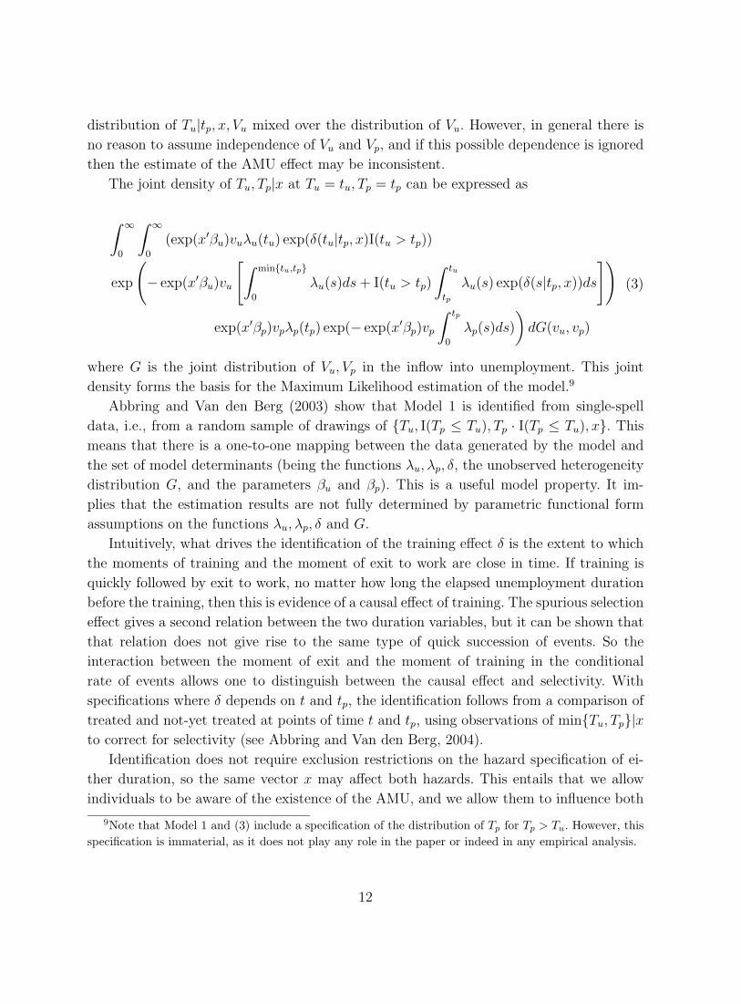
The joint density of Tu, Tp|x at Tu = tu, Tp = tp can be expressed as
∫ ∞
0
∫ ∞
0
(exp(x′βu)vuλu(tu) exp(δ(tu|tp, x)I(tu > tp))
exp
(− exp(x′βu)vu
[∫ min{tu,tp}
0
λu(s)ds+ I(tu > tp)
∫ tu
tp
λu(s) exp(δ(s|tp, x))ds])
exp(x′βp)vpλp(tp) exp(− exp(x′βp)vp
∫ tp
0
λp(s)ds)
)dG(vu, vp)
(3)
where G is the joint distribution of Vu, Vp in the inflow into unemployment. This joint
density forms the basis for the Maximum Likelihood estimation of the model.9
Abbring and Van den Berg (2003) show that Model 1 is identified from single-spell
data, i.e., from a random sample of drawings of {Tu, I(Tp ≤ Tu), Tp · I(Tp ≤ Tu), x}. Thismeans that there is a one-to-one mapping between the data generated by the model and
the set of model determinants (being the functions λu, λp, δ, the unobserved heterogeneity
distribution G, and the parameters βu and βp). This is a useful model property. It im-
plies that the estimation results are not fully determined by parametric functional form
assumptions on the functions λu, λp, δ and G.
Intuitively, what drives the identification of the training effect δ is the extent to which
the moments of training and the moment of exit to work are close in time. If training is
quickly followed by exit to work, no matter how long the elapsed unemployment duration
before the training, then this is evidence of a causal effect of training. The spurious selection
effect gives a second relation between the two duration variables, but it can be shown that
that relation does not give rise to the same type of quick succession of events. So the
interaction between the moment of exit and the moment of training in the conditional
rate of events allows one to distinguish between the causal effect and selectivity. With
specifications where δ depends on t and tp, the identification follows from a comparison of
treated and not-yet treated at points of time t and tp, using observations of min{Tu, Tp}|xto correct for selectivity (see Abbring and Van den Berg, 2004).
Identification does not require exclusion restrictions on the hazard specification of ei-
ther duration, so the same vector x may affect both hazards. This entails that we allow
individuals to be aware of the existence of the AMU, and we allow them to influence both
9Note that Model 1 and (3) include a specification of the distribution of Tp for Tp > Tu. However, thisspecification is immaterial, as it does not play any role in the paper or indeed in any empirical analysis.
12
the rate of entry into AMU and the rate of exit into employment. This is obviously an
advantage. We return to this below.
So far we have ignored time-varying covariates, although tp can be thought of as an
endogenous time-varying covariate in θu. It is clear that in some cases a model with time-
varying covariates is not identified, for example, if θi(t|x, vi) = λi(t) exp(x(t)′βi) with x(t)
additive in t. However, in general, variation of x over time is helpful for identification of
duration models. Honore (1991) and Heckman and Taber (1994) provide some illustrations
of this. In our empirical model specifications we include exogenous x variables that vary
over time.
The identification with single-spell data does require a number of assumptions that
are standard in the literature on identification of MPH models. Notably, X⊥⊥ V , and Xincludes two continuous variables with the properties that (i) their joint support contains
a non-empty open set in R2, and (ii) the vectors of the corresponding elements of βu
and βp form a matrix of full rank. Abbring and Van den Berg (2003) show that these
assumptions can be discarded if the data provide multiple spells, i.e. if for individuals in
the sample we have more than one unemployment spell with the same value of V , and if
these spells are independent given the values of x and V . We assume that an individual
has a given value of Vu, Vp. Since Vu and Vp are unobserved, the duration variables given x
are not independent across spells. It is especially useful that identification with multi-spell
data does not require independence of observed and unobserved explanatory variables, as
in general such independence is hard to justify. In fact, multi-spell data also allow the
relaxation of multiplicity assumptions in Model 1. Specifically, we may allow x to enter in
an arbitrary nonproportional manner in the conditional hazard rates, and we do not need
variation of these hazard rates with x at all. Alternatively, we may allow the dependence of
the conditional hazard rates on t, x in the second spell to be different from the dependence
of these rates on t, x in the first spell. The size of the AMU effect may also be different
across the two spells. A causal effect of the realizations for the first spell on the outcomes for
the second spell or the other way round is not allowed (although the observed outcomes are
related across spells by way of their unobserved determinants). But the individual values
of x may differ across spells.
3.2 Identification of models with duration dependence and un-
observed heterogeneity in the treatment effect
In the model of the previous subsection, the magnitude of the causal training effect δ does
not depend on unobserved characteristics, so any systematic heterogeneity of treatment
effects across individuals comes from observable characteristics x. It is hard to justify this
assumption. Moreover, unobserved heterogeneity in δ may be an important explanation
13
for changes of the observed (i.e., only conditional on x) treatment effect over time. The
intuition is the same as for the spurious duration dependence generated by unobserved het-
erogeneity in duration models (e.g. Lancaster, 1990). Treated individuals with unobserved
characteristics such that their treatment effect is high are (holding every other character-
istic constant) more likely to leave unemployment quickly.10 This tends to decrease the
average treatment effect among the treated survivors. Of course, if the unobserved charac-
teristics affecting the treatment effect are inversely related to the unobserved characteristics
Vu affecting the exit rate to work in general, then more subtle effects can be generated for
the observed treatment effect.
As we shall see in Section 4, the decline of the observed exit rate to work among
the treated is a major distinguishing feature of the raw data. It therefore makes sense to
consider models that allow for both duration dependence of the individual treatment effect
and spurious duration dependence due to dynamic selection as two potential explanations
for the observed decline. Moreover, whether the exit rate after treatment declines because
of a fading treatment effect or because of dynamic selection has major policy implications.
In the former case the policy is only effective for a short while, whereas in the latter case
one might want to screen individuals more closely before admission into training.
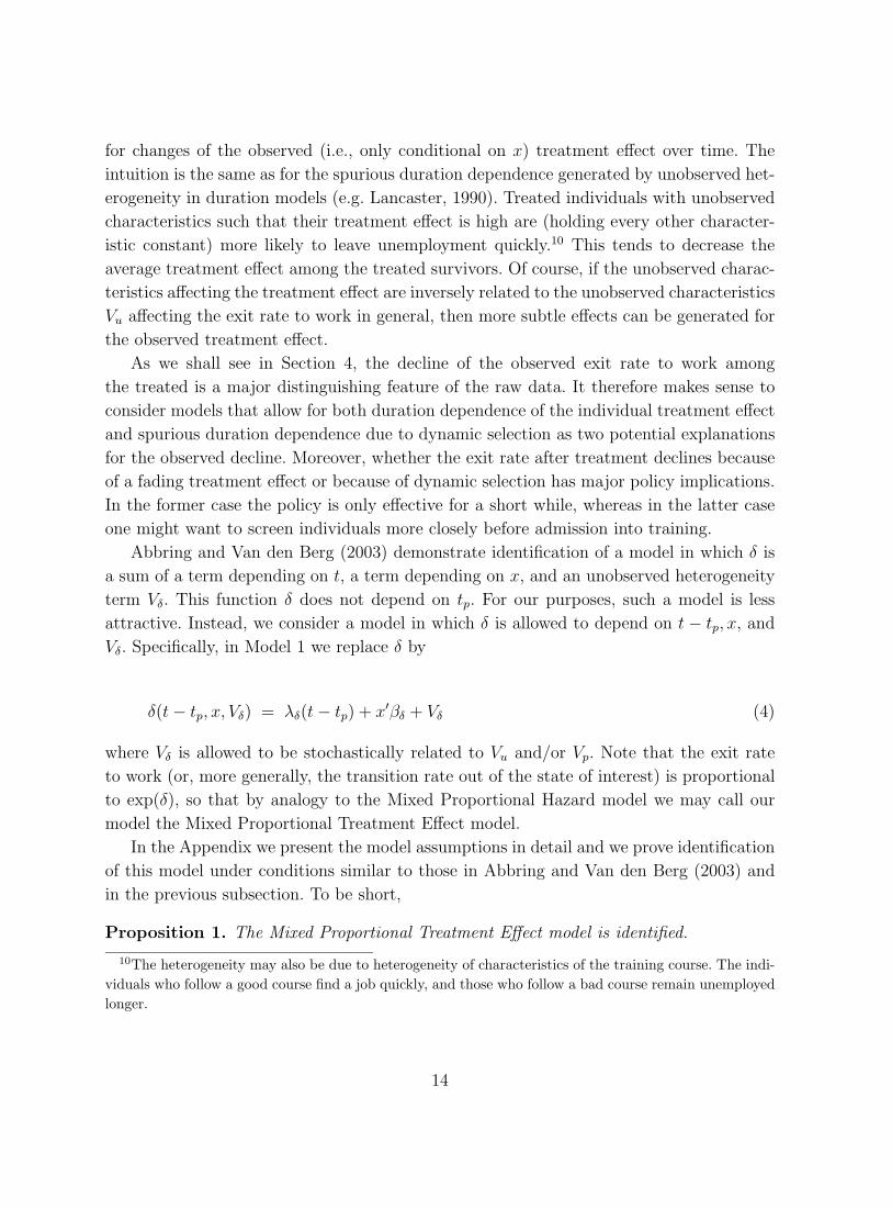
Abbring and Van den Berg (2003) demonstrate identification of a model in which δ is
a sum of a term depending on t, a term depending on x, and an unobserved heterogeneity
term Vδ. This function δ does not depend on tp. For our purposes, such a model is less
attractive. Instead, we consider a model in which δ is allowed to depend on t − tp, x, andVδ. Specifically, in Model 1 we replace δ by
δ(t− tp, x, Vδ) = λδ(t− tp) + x′βδ + Vδ (4)
where Vδ is allowed to be stochastically related to Vu and/or Vp. Note that the exit rate
to work (or, more generally, the transition rate out of the state of interest) is proportional
to exp(δ), so that by analogy to the Mixed Proportional Hazard model we may call our
model the Mixed Proportional Treatment Effect model.
In the Appendix we present the model assumptions in detail and we prove identification
of this model under conditions similar to those in Abbring and Van den Berg (2003) and
in the previous subsection. To be short,
Proposition 1. The Mixed Proportional Treatment Effect model is identified.
10The heterogeneity may also be due to heterogeneity of characteristics of the training course. The indi-viduals who follow a good course find a job quickly, and those who follow a bad course remain unemployedlonger.
14
3.3 Implicit assumptions in the model specifications
The model specifications reflect a number of implicit assumptions. First of all, the future
realization of the moment tp of entry into training does not affect the individual’s exit rate
θu prior to that moment tp. So the individual’s exit rate at t is the same irrespective of
whether training will occur at t + 1 or whether it will occur at t + 100. This rules out
anticipation of the future individual realization of the moment of training. If an individual
would foresee participation in AMU at a particular future date tp then he may use this
as an input of his current behavior, for example he may want to wait for the treatment
by reducing his search intensity for jobs, and this may decrease the probability that Tu
is quickly realized. If this is ignored in the empirical analysis then the training effect
may be over-estimated. However, if the time span between the earliest moment at which
anticipation can occur and the moment of the actual training is short relative to typical
values of the durations Tp and Tu −Tp, and if the anticipatory effect is not very large, then
estimation results may be relatively insensitive to the assumption of no anticipation.
It is important to distinguish anticipation of the realization of Tp from ex ante knowl-
edge of the existence of the program and ex ante knowledge of the individual distribution
of Tp. With well-established programs like AMU, it is plausible that determinants of the
stochastic process of training assignment affect the individual’s exit rate out of unemploy-
ment before the actual entry into training. For example, if the individual knows that he
has a relatively high training enrolment rate and if he enjoys training then he will reduce
his job search effort. In such cases the program is said to have an ex ante effect on exit
out of unemployment before training. The “ex ante” effect contrasts to the ex post effect
of training, which is the effect of actual training on the individual exit rate. The ex ante
effect is an example of the macro effects that are present in a world in which a particular
program is implemented. There may also be ex ante or macro effects on the magnitude
and composition on the inflow into unemployment and on the behavior of employers.
The model framework is compatible with ex ante effects. However, we do not aim to
disentangle such effects from other determinants of the hazard rates. Identification of the ex
ante effect on the exit rate to work before training requires additional information, such as
strong functional-form assumptions, instruments for a comparison of a world with AMU to
a world without it, or the imposition of an economic-theoretic structure on the model (see
Abbring and Van den Berg, 2005). The first option is undesirable, whereas the others are
beyond the scope of this paper. This means that the treatment effect δ is defined relative
to the exit rate to work in absence of a treatment but within a world in which treatments
are present.
We now turn to a different type of anticipation. The model framework rules out that
the future realization of the variable of interest Tu has an effect on the current level of θp.
In reality, an individual may have private knowledge on a future job opportunity that is
15
independent of whether the training will occur, and the individual may use this knowledge
to avoid training. If something like does occur in reality then a positive effect of training
on exit to employment is under-estimated. However, if the training course takes a long
time, then this bias may be empirically unimportant, as employers may be unwilling to
wait for a new employee for many months. Also, if the time span between the moment
at which the anticipation occurs and the moment of the actual exit to work is relatively
short, and if the anticipatory effect is not very large, then estimation results may be rather
insensitive to this. Again, absence of anticipation does not rule out that individuals know
the determinants of the process leading to employment and use these as inputs in their
decision problem. For example, the individuals may know that λu(t) increases in the near
future, and modify their strategy accordingly, which may affect their θp. The latter can be
captured in the model through λp(t).
Finally, the fact that we specify the assignment of training by way of specifying the
hazard rate of a duration distribution implies that there is a random component in the
assignment that is independent of all other variables (see e.g. Ridder, 1990, and Abbring
and Van den Berg, 2003). The model framework thus postulates that there is variation in
Tp at the individual level. (This variation affects Tu only by way of the treatment.) To see
the importance of this, consider the extreme case where individuals can only enter AMU at,
say, exactly one year after flowing into unemployment. Then it is impossible to distinguish
the effect of AMU from the duration dependence in the exit rate to work after one year.
(In such a case it is of course also hard to justify that entry into AMU is not anticipated.)
3.4 Applicability of the model framework to AMU
In this subsection we argue that the model framework (covering the different specifications
we consider) is particularly well suited for our study of the AMU program. We focus on
the following issues: dependent unobserved heterogeneity, randomness in the moment of
treatment assignment, absence of anticipatory effects, and absence of substitution with
other programs.
From the information in Subsection 2.2 and from the studies by Eriksson (1997a, 1997b),
it is obvious that unobserved (to us) heterogeneity of the unemployed individuals plays an
important role in the assignment to AMU. The corresponding variables taken into account
by the caseworker (like motivation, subjectively assessed expected unemployment duration,
and subjective assessments of other aspects of the future career) are also indicative of
unobserved determinants of the individual exit rate to work. The empirical analysis should
therefore take account of potentially related unobserved heterogeneity terms in θu and θp.
If the individual knows that a variable is an important determinant of the treatment
assignment process (like the amount and type of discretionary behavior of his caseworker),
16
and the individual knows that he may be subject to treatment, then he has a strong
incentive to inquire the actual value of the variable. Subsequently, he will take his value
of the variable into account to determine his optimal strategy, and this strategy in turn
affects the rate at which he moves to employment. We should note that the variables that
are observed by us and that may have an effect on assignment to AMU are also observable
to the individuals under consideration, so that we cannot impose exclusion restrictions on
βu, and we take the same vector x to affect both θu and θp.
Now let us consider the presence of randomness in the moment of entry into AMU.
To some extent this may be generated by changes in the behavior of the caseworker or
the employment agency that are beyond observation of the unemployed individual. More
importantly, it is generated by the variation in the moment at which AMU courses start. In
addition, admission to a course may depend on the extent to which other individuals apply
to the course, which is random from the individual’s point of view. Recall that Eriksson
(1997b) finds residual variation in the AMU assignment process that can not be attributed
to the individual or the caseworker.
We now turn to anticipation of the moment of entry into AMU. From Subsection 2.2, the
time period between the moment at which the individual is informed about the possibility
of enrolling into an AMU course and the moment at which the course starts is very short.
There are however two reasons for why some individuals may anticipate the moment of
entry, and both of these lead us to restrict the focus of the empirical analysis somewhat.
First, as discussed in Section 2, in 1991 and 1992 AMU was often used to extend benefits
entitlement. In that case, the date of inflow into AMU is mostly determined by the date of
expiration of benefits entitlement. The latter date is known in advance by the unemployed
individual and his caseworker (this date does not vary much across the unemployed; see
the references). This allows for anticipation of the inflow into AMU, which violates a key
assumption of our evaluation approach. Moreover, such self-selection into AMU is governed
by different motives than self-selection in other years, so we may expect the unobserved
heterogeneity distribution to be different across time. From January 1993 onwards, other
programs took over its role as means to extend benefits entitlement. We therefore restrict
attention to data from 1993 onwards.
Secondly, recall from Section 2 that part of AMU concerns non-vocational training,
in particular before 1997. Non-vocational training is often given within the regular school
system. This implies that the starting date of the non-vocational training is often deter-
mined by institutional features of the school system, like the starting dates of the school
seasons. As a result, it is straightforward for unemployed individuals to anticipate the date
of inflow into such a program. We therefore restrict ourselves to vocational training. There
are two additional reasons to do so. First, vocational training is relatively expensive, so the
participation costs are higher. Secondly, vocational training is difficult to obtain in alterna-
17
tive labor market programs, whereas non-vocational training is easier to obtain elsewhere,
implying that in the latter case there are substitution possibilities.
Concerning substitution possibilities in general, recall from Subsection 2.2 that case
workers regard vocational AMU training as a very different type of program than the
other active labor market programs. The latter are regarded to be substitutable to a high
degree. For persons under 25, there are programs that are more similar to AMU vocational
training. Also, for these individuals, the similarity with vocational courses and tracks in
the regular school system may be important. For this reason we restrict attention to indi-
viduals aged over 25. Also, young individuals must enter a training course after 100 days of
unemployment, which may generate anticipatory effects. We omit individuals over 55 be-
cause they face a different unemployment benefits system and because for them vocational
AMU training seems to have relatively small advantages.
It follows from the above that our model framework may be less suited for the analysis
of the effects of the other active labor market programs on unemployment duration. With
other programs, individuals may anticipate their enrolment a long time in advance, because
of their link to benefits entitlement expiration and/or because of their connection to the
regular school system. Moreover, it is difficult to analyze them in isolation from each other
because of the high degree of substitutability.
4 The data
4.1 Data registers and unemployment spells
The data are taken from a combination of two Swedish register data sets called HANDEL
(from the official employment offices) and AKSTAT (from the unemployment insurance
fund). HANDEL covers all registered unemployed persons since August 1991 (approxi-
mately 2 million observations). According to Carling, Holmlund and Vejsiu (2001), more
than 90are ILO-unemployed according to labor force surveys also register at the employ-
ment offices. HANDEL includes detailed information on the individuals’ training activities
and work experience activities, including the starting and ending dates of program partici-
pation. HANDEL is also informative on whether an individual in AMU receives vocational
training or non-vocational training. AKSTAT is available from 1994 onwards and provides
information on the wage level and working hours in the job prior to the spell of unemploy-
ment, for individuals who are eligible for UI.
Our observation window runs from January 1, 1993 until June 22, 2000. The unit of
observation is an individual. For each individual who is in HANDEL at least once during
the observation window, we can construct an event history from HANDEL. For any spell
of unemployment (to be defined below), HANDEL and AKSTAT provide characteristics
18
at the beginning of the spell, and a list of dates within the spell at which changes occur,
including the nature of the change. We also include the information on participation in
non-AMU programs, since such participation may temporarily rule out a transition to
AMU, or may at least reduce the transition rate to AMU and/or work.
We only use information on individuals who become unemployed at least once within
the observation window. An individual becomes unemployed at the first date at which he
registers at the employment office as being “openly” unemployed. This eliminates registra-
tion spells that start because the individual wants to change employer and also eliminates
spells that start because the individual knows that he is going to be unemployed in the
future (short term contract or notification of lay-off), at least until the individual does
actually become unemployed. We also ignore unemployment spells that are already in
progress at the beginning of the observation window, because using them would force us
to make assumptions about the period before the beginning of the window. We thus ob-
tain a so-called inflow sample of unemployment spells, and we follow the individuals over
time after this moment of inflow. (Note that we also use information available on the pe-
riod prior to such spells, notably on wages.) We exclude individuals who have experienced
unemployment between August 1991 and January 1, 1993. The years 1990–1992 witness
an unusually severe recession in Sweden, and the individuals who became unemployed in
that period may be different from those who did not become unemployed then but who
became unemployed later. As we have seen, the former individuals were certainly exposed
to a different active labor market policy regime before 1993, and this might affect their
outcomes after 1993 as well.
For convenience, we use the term “unemployment spell” to include possible spells in
AMU, relief work, ALU, etc. The spell ends if the individual leaves the employment office
register or if he moves from the unemployment categories in the employment office register
to a non-unemployment category in the register. If the exit destination is employment
then we observe a realization of the duration variable of interest. If the exit destination
is different (e.g. “regular education”, or “other reason”) then this duration variable is
right-censored (independence of right-censoring may be checked in a sensitivity analysis).
The duration is independent right-censored if the spell is continuing at the end of the
observation window.
Occasionally, we observe coding errors in data at points of time at which individuals
move between different categories in the register. Obvious typing errors are corrected,
whereas otherwise we right-censor the duration variables at the moment at which such an
error occurs. If exit occurs into “wage subsidy” or “(public) sheltered employment” then we
remove the individual from the sample, since these programs are for handicapped people
(who are typically are not in open unemployment anyway). As mentioned in Subsection
3.4, we restrict attention to individuals who were at least 25 and below 55 at the moment
19
they enter unemployment. As a result, our data set contains 500,960 individuals. Note
that by following the individuals over time we may observe multiple unemployment spells
per individual. For each individual we use at most 3 unemployment spells. The analyses
are based on a random subsample of the full data set at our disposal, containing 16467
individuals, with in total 28451 unemployment spells.
Even though vocational AMU and other programs are fundamentally different and are
not used as substitutes, we are forced to consider the participation in other programs
during unemployment, as such participation spells are likely to affect the transition rates
into AMU and into work for a certain amount of time. Since participation in those other
programs takes place at points in time that are dispersed across individuals and that may
to some extent be random, the common deterministic duration dependence functions in
Model 1 cannot capture this. Also, we have seen that expanding the Timing of Events
model framework to include multiple types of treatment is hard to justify. If we treat par-
ticipation in other programs before participation in AMU as regular unemployment, then
the transition rate from unemployment into AMU is extremely low during the participation
in the other programs. Participation in non-AMU programs most likely also reduces the
transition rate into employment. So, during such a period of program participation, it may
be preferable to halt the time clock of the duration until regular employment. As a starting
point, the time spent in training (in non-AMU programs as well as in AMU) is therefore
assumed not to contribute to the unemployment duration, and the time spent in other
training programs is assumed not to contribute to the duration until AMU. Note that this
also means that time spent in non-AMU programs after AMU does not contribute to the
unemployment duration. We subsequently relax these assumptions in additional analyses.
4.2 Descriptive statistics
Table 1 provides summary statistics of the unemployment duration, the participation in
labor market programs, and their interrelation. Of all 28451 spells, 2185 (i.e. 7.7%) are
observed to include a period of participation in a vocational AMU course. Some of the
other spells are right-censored due to the finiteness of the observation window, and in
reality some of those may include AMU participation afterwards. The median value of the
duration until training across the 2185 spells that are observed to include training is 153
days. Except where stated otherwise, the duration outcomes in Table 1 are measured while
ignoring time in training and other programs.
In a setting where one duration outcome of interest (Tp) is right-censored by the other
(Tu) and both durations are subject to end-of-follow-up right-censoring, the information
in summary statistics of outcomes is limited. Spells with observed AMU participation are
longer than spells without simply because it takes time before Tp is realized. To complicate
20
matters further, note that right-censoring due to finiteness of the observation window takes
place at the duration value equal to the difference between June 22, 2000, and the moment
of inflow into unemployment, and the latter is dispersed across spells. One notable aspect
is that a sizeable fraction of spells with AMU participation ends with a transition to work
within a few days after leaving training.
Of the 2185 spells that are observed to include AMU participation, 47% are also ob-
served to include participation in another type of active labor market program. Not sur-
prisingly, this happens predominantly in long spells. Of the spells with tp smaller than 160
days, only 12% are also observed to include participation in another type of active labor
market program before AMU participation. Of the spells observed to be shorter than 160
days that are not observed to include participation in AMU, 10% are observed to include
participation in another type of active labor market program. This suggests that participa-
tion in other programs is not related to AMU participation. The fact that spells with AMU
participation relatively often also include participation in other programs is because of the
fact that by conditioning on AMU participation we condition on high realized durations.
Table 2 provides summary statistics of explanatory variables in the empirical analysis,
across all spells and across all first spells. The latter reflects the composition across indi-
viduals better than the former, as we allow the x variables to differ across the spells of a
given individual.
Concerning education we distinguish between five levels: junior high school or lower,
short senior high school, long senior high school, short tertiary education, and full university
degree or higher. These are roughly equivalent to ≤ 9, 10–11, 12–13, 14, and ≥ 15 years
of education, respectively. Concerning nationality we distinguish between three categories:
Eastern Europe, Africa / Asia, and otherwise (including Sweden). Concerning the type
of unemployment benefits received during unemployment we distinguish between three
categories: UI, cash allowance, and neither. For UI recipients in 1994 and beyond, the
AKSTAT data include the hourly wage earned in the job that was held just before the
onset of the spell of unemployment. This is almost linearly related to their UI level (see e.g.
Carling, Holmlund and Vejsiu, 2001). For non-UI-recipients the wage variable is set to zero.
The latter also applies to UI recipients who become unemployed and subsequently employed
within 1993. However, if they move back to unemployment in 1994 we use the corresponding
pre-unemployment wage to quantify the pre-unemployment wage for the unemployment
spell in 1993. The “large city” dummy equals 1 iff the individual lives in one of the counties
covering Stockholm, Goteborg, and Malmo. Notice that some variables concern subjective
assessments by the case worker (e.g. whether the individual needs guidance) or subjective
statements by the individual concerning the span of jobs that he searches for.
The sample means across spells are virtually equal to those across individuals in their
first spell. This suggests that the observation of multiple spells is not strongly driven by
21
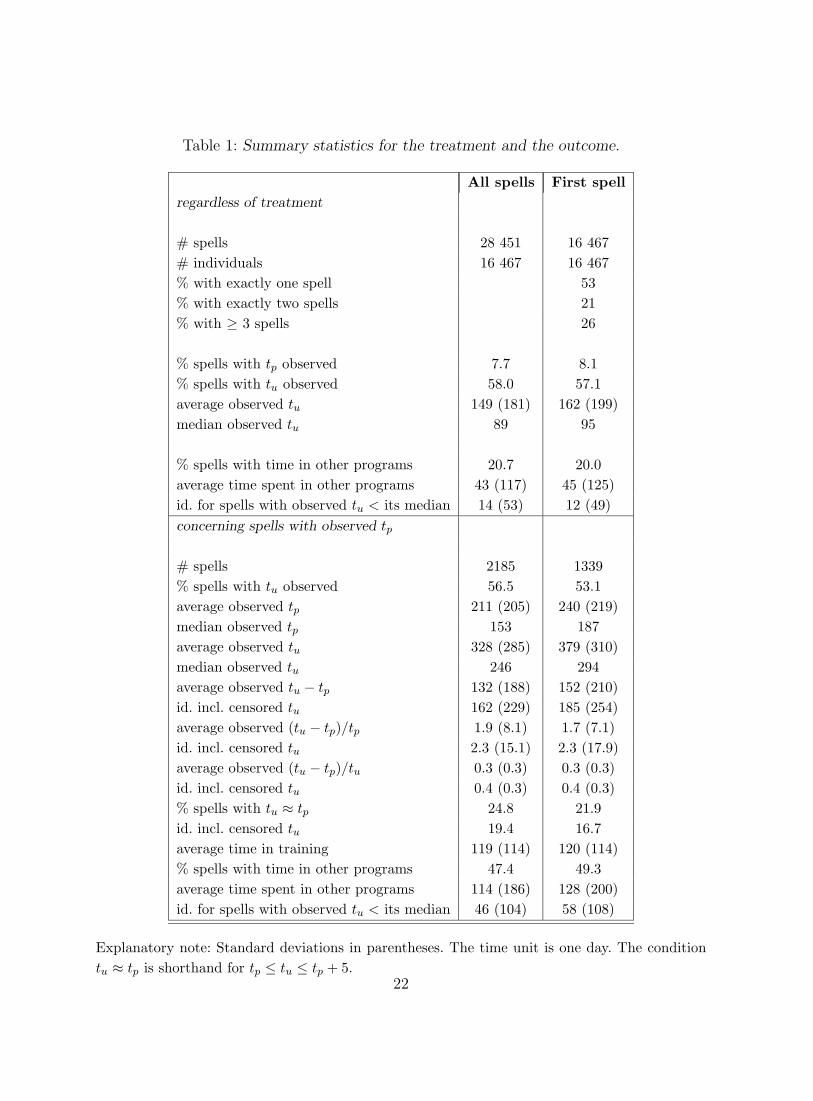
Table 1: Summary statistics for the treatment and the outcome.
All spells First spellregardless of treatment
# spells 28 451 16 467# individuals 16 467 16 467% with exactly one spell 53% with exactly two spells 21% with ≥ 3 spells 26
% spells with tp observed 7.7 8.1% spells with tu observed 58.0 57.1average observed tu 149 (181) 162 (199)median observed tu 89 95
% spells with time in other programs 20.7 20.0average time spent in other programs 43 (117) 45 (125)id. for spells with observed tu < its median 14 (53) 12 (49)concerning spells with observed tp
# spells 2185 1339% spells with tu observed 56.5 53.1average observed tp 211 (205) 240 (219)median observed tp 153 187average observed tu 328 (285) 379 (310)median observed tu 246 294average observed tu − tp 132 (188) 152 (210)id. incl. censored tu 162 (229) 185 (254)average observed (tu − tp)/tp 1.9 (8.1) 1.7 (7.1)id. incl. censored tu 2.3 (15.1) 2.3 (17.9)average observed (tu − tp)/tu 0.3 (0.3) 0.3 (0.3)id. incl. censored tu 0.4 (0.3) 0.4 (0.3)% spells with tu ≈ tp 24.8 21.9id. incl. censored tu 19.4 16.7average time in training 119 (114) 120 (114)% spells with time in other programs 47.4 49.3average time spent in other programs 114 (186) 128 (200)id. for spells with observed tu < its median 46 (104) 58 (108)
Explanatory note: Standard deviations in parentheses. The time unit is one day. The conditiontu ≈ tp is shorthand for tp ≤ tu ≤ tp + 5.
22
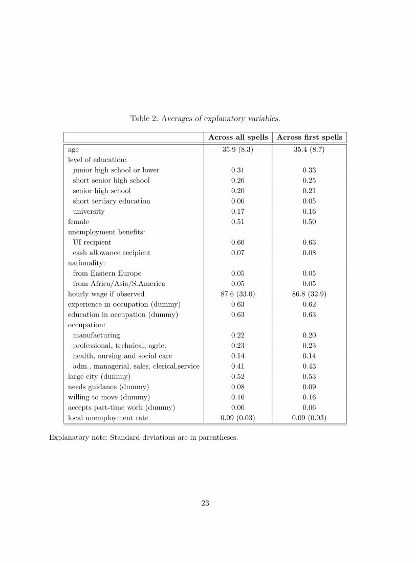
Table 2: Averages of explanatory variables.
Across all spells Across first spells
age 35.9 (8.3) 35.4 (8.7)level of education:junior high school or lower 0.31 0.33short senior high school 0.26 0.25senior high school 0.20 0.21short tertiary education 0.06 0.05university 0.17 0.16
female 0.51 0.50unemployment benefits:UI recipient 0.66 0.63cash allowance recipient 0.07 0.08
nationality:from Eastern Europe 0.05 0.05from Africa/Asia/S.America 0.05 0.05
hourly wage if observed 87.6 (33.0) 86.8 (32.9)experience in occupation (dummy) 0.63 0.62education in occupation (dummy) 0.63 0.63occupation:manufacturing 0.22 0.20professional, technical, agric. 0.23 0.23health, nursing and social care 0.14 0.14adm., managerial, sales, clerical,service 0.41 0.43
large city (dummy) 0.52 0.53needs guidance (dummy) 0.08 0.09willing to move (dummy) 0.16 0.16accepts part-time work (dummy) 0.06 0.06local unemployment rate 0.09 (0.03) 0.09 (0.03)
Explanatory note: Standard deviations are in parentheses.
23
selectivity. Age is on average slightly higher across spells than across individuals in their
first spell, but this is a consequence of the fact that an individual’s age necessarily increases
over consecutive spells.
5 The empirical analysis
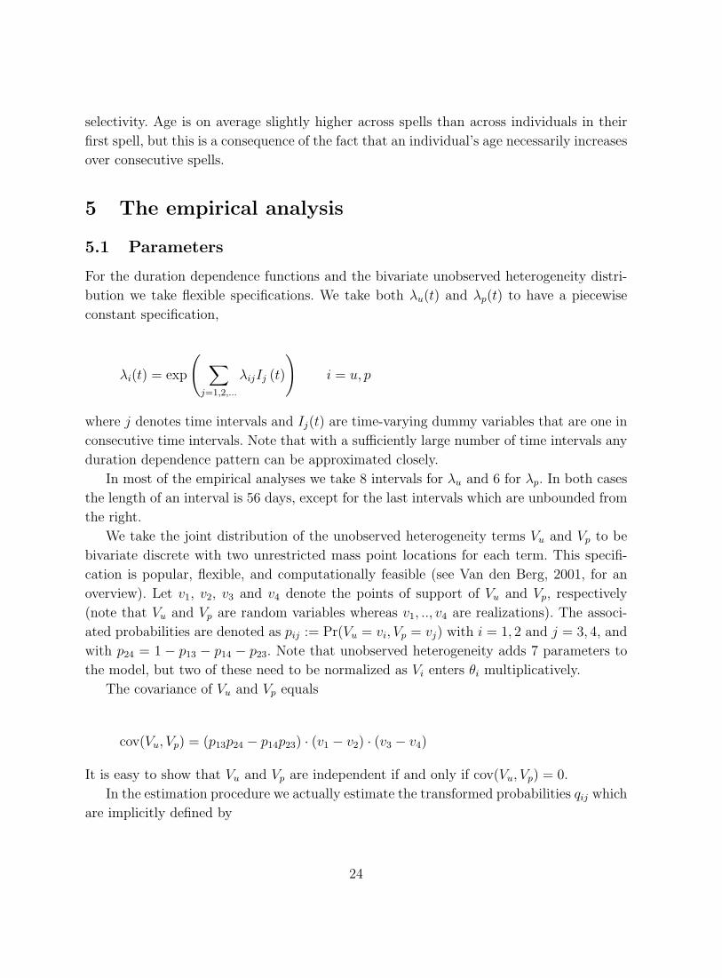
5.1 Parameters
For the duration dependence functions and the bivariate unobserved heterogeneity distri-
bution we take flexible specifications. We take both λu(t) and λp(t) to have a piecewise
constant specification,
λi(t) = exp
( ∑j=1,2,...
λijIj (t)
)i = u, p
where j denotes time intervals and Ij(t) are time-varying dummy variables that are one in
consecutive time intervals. Note that with a sufficiently large number of time intervals any
duration dependence pattern can be approximated closely.
In most of the empirical analyses we take 8 intervals for λu and 6 for λp. In both cases
the length of an interval is 56 days, except for the last intervals which are unbounded from
the right.
We take the joint distribution of the unobserved heterogeneity terms Vu and Vp to be
bivariate discrete with two unrestricted mass point locations for each term. This specifi-
cation is popular, flexible, and computationally feasible (see Van den Berg, 2001, for an
overview). Let v1, v2, v3 and v4 denote the points of support of Vu and Vp, respectively
(note that Vu and Vp are random variables whereas v1, .., v4 are realizations). The associ-
ated probabilities are denoted as pij := Pr(Vu = vi, Vp = vj) with i = 1, 2 and j = 3, 4, and
with p24 = 1 − p13 − p14 − p23. Note that unobserved heterogeneity adds 7 parameters tothe model, but two of these need to be normalized as Vi enters θi multiplicatively.
The covariance of Vu and Vp equals
cov(Vu, Vp) = (p13p24 − p14p23) · (v1 − v2) · (v3 − v4)
It is easy to show that Vu and Vp are independent if and only if cov(Vu, Vp) = 0.
In the estimation procedure we actually estimate the transformed probabilities qij which
are implicitly defined by
24
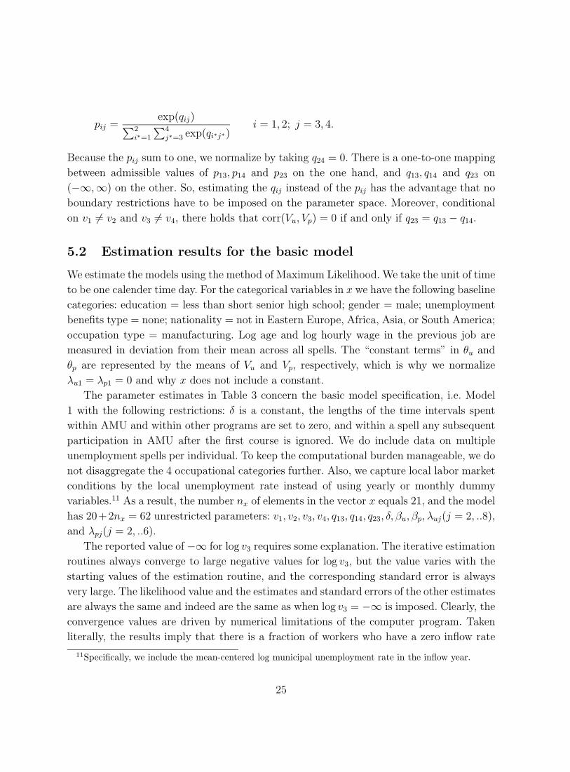
pij =exp(qij)∑2
i∗=1
∑4j∗=3 exp(qi∗j∗)
i = 1, 2; j = 3, 4.
Because the pij sum to one, we normalize by taking q24 = 0. There is a one-to-one mapping
between admissible values of p13, p14 and p23 on the one hand, and q13, q14 and q23 on
(−∞,∞) on the other. So, estimating the qij instead of the pij has the advantage that no
boundary restrictions have to be imposed on the parameter space. Moreover, conditional
on v1 �= v2 and v3 �= v4, there holds that corr(Vu, Vp) = 0 if and only if q23 = q13 − q14.
5.2 Estimation results for the basic model
We estimate the models using the method of Maximum Likelihood. We take the unit of time
to be one calender time day. For the categorical variables in x we have the following baseline
categories: education = less than short senior high school; gender = male; unemployment
benefits type = none; nationality = not in Eastern Europe, Africa, Asia, or South America;
occupation type = manufacturing. Log age and log hourly wage in the previous job are
measured in deviation from their mean across all spells. The “constant terms” in θu and
θp are represented by the means of Vu and Vp, respectively, which is why we normalize
λu1 = λp1 = 0 and why x does not include a constant.
The parameter estimates in Table 3 concern the basic model specification, i.e. Model
1 with the following restrictions: δ is a constant, the lengths of the time intervals spent
within AMU and within other programs are set to zero, and within a spell any subsequent
participation in AMU after the first course is ignored. We do include data on multiple
unemployment spells per individual. To keep the computational burden manageable, we do
not disaggregate the 4 occupational categories further. Also, we capture local labor market
conditions by the local unemployment rate instead of using yearly or monthly dummy
variables.11 As a result, the number nx of elements in the vector x equals 21, and the model
has 20+2nx = 62 unrestricted parameters: v1, v2, v3, v4, q13, q14, q23, δ, βu, βp, λuj(j = 2, ..8),
and λpj(j = 2, ..6).
The reported value of −∞ for log v3 requires some explanation. The iterative estimation
routines always converge to large negative values for log v3, but the value varies with the
starting values of the estimation routine, and the corresponding standard error is always
very large. The likelihood value and the estimates and standard errors of the other estimates
are always the same and indeed are the same as when log v3 = −∞ is imposed. Clearly, the
convergence values are driven by numerical limitations of the computer program. Taken
literally, the results imply that there is a fraction of workers who have a zero inflow rate
11Specifically, we include the mean-centered log municipal unemployment rate in the inflow year.
25
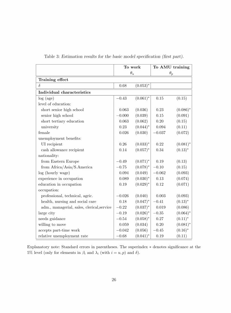
Table 3: Estimation results for the basic model specification (first part).
To work To AMU trainingθu θp
Training effectδ 0.68 (0.053)∗
Individual characteristicslog (age) −0.43 (0.061)∗ 0.15 (0.15)level of education:short senior high school 0.063 (0.036) 0.23 (0.086)∗
senior high school −0.000 (0.039) 0.15 (0.091)short tertiary education 0.063 (0.062) 0.20 (0.15)university 0.23 (0.044)∗ 0.094 (0.11)
female 0.026 (0.030) −0.037 (0.072)unemployment benefits:UI recipient 0.26 (0.033)∗ 0.22 (0.081)∗
cash allowance recipient 0.14 (0.057)∗ 0.34 (0.13)∗
nationality:from Eastern Europe −0.49 (0.071)∗ 0.19 (0.13)from Africa/Asia/S.America −0.75 (0.078)∗ −0.10 (0.15)
log (hourly wage) 0.094 (0.049) −0.062 (0.093)experience in occupation 0.089 (0.030)∗ 0.13 (0.074)education in occupation 0.19 (0.029)∗ 0.12 (0.071)occupation:professional, technical, agric. −0.026 (0.040) 0.003 (0.093)health, nursing and social care 0.18 (0.047)∗ −0.41 (0.13)∗
adm., managerial, sales, clerical,service −0.22 (0.037)∗ 0.019 (0.086)large city −0.19 (0.026)∗ −0.35 (0.064)∗
needs guidance −0.54 (0.058)∗ 0.27 (0.11)∗
willing to move 0.059 (0.034) 0.20 (0.081)∗
accepts part-time work −0.042 (0.056) −0.45 (0.16)∗
relative unemployment rate −0.68 (0.041)∗ 0.19 (0.11)
Explanatory note: Standard errors in parentheses. The superindex ∗ denotes significance at the5% level (only for elements in βi and λi (with i = u, p) and δ).
26
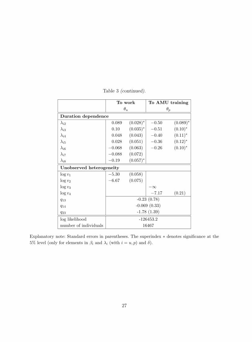
Table 3 (continued).
To work To AMU trainingθu θp
Duration dependenceλi2 0.089 (0.028)∗ −0.50 (0.089)∗
λi3 0.10 (0.035)∗ −0.51 (0.10)∗
λi4 0.048 (0.043) −0.40 (0.11)∗
λi5 0.028 (0.051) −0.36 (0.12)∗
λi6 −0.068 (0.063) −0.26 (0.10)∗
λi7 −0.088 (0.072)λi8 −0.19 (0.057)∗
Unobserved heterogeneitylog v1 −5.30 (0.058)log v2 −6.67 (0.075)log v3 −∞log v4 −7.17 (0.21)q13 -0.23 (0.78)q14 -0.069 (0.33)q23 -1.78 (1.39)
log likelihood -126453.2number of individuals 16467
Explanatory note: Standard errors in parentheses. The superindex ∗ denotes significance at the5% level (only for elements in βi and λi (with i = u, p) and δ).
27
into training. This may be true, or it may be that the actual inflow rate is a small positive
number.
The main parameter of interest is the causal effect δ of training on the transition rate
to work. The estimated value of δ is 0.68 and is significantly different from 0. Training
thus raises this transition rate with about 100%, which means that it doubles. The effect
on the mean or median unemployment duration depends on the moment at which training
occurs. If the training is given within the first month then the mean duration is more or
less reduced by half. Similarly, training at a relatively early stage in an unemployment
spell has a large effect on the probability of long-term unemployment. (Of course, such a
policy can be costly if implemented on a wide scale.) Recall that (part of) the effect may
be due to increased search effort on the part of the caseworker, both before and during the
participation period.
Now let us turn to the covariate effects βu and duration dependence λu of the transition
rate to work. To the extent that they are also estimated in other studies on recent Swedish
unemployment durations, like Carling, Holmlund and Vejsiu (2001), the results are similar
to those reported in those studies. The signs of the significant covariate effects are as ex-
pected. The exit rate to work is significantly lower for older and non-Swedish individuals
and higher for university graduates. It is also higher for unemployment benefits recipients,
reflecting the stronger labor market attachment of these individuals. There are no signifi-
cant disincentive effect of high benefits as represented by the previous wage. Note however
that this variable presumably also captures the mean wage offer. Individuals in large cities
and in areas and years with high unemployment have a lower exit rate to work, whereas
individuals with experience in their occupation or with an education that fits in with their
occupation have a higher rate. Finally, individuals deemed to be in need of guidance by the
case worker at the moment of entry into unemployment have a much lower exit rate than
others. This captures characteristics of the individual that are not fully described by the
observed explanatory variables. The estimated duration dependence of θu is such that the
individual transition rate to work decreases as the duration increases. Apparently, stigma-
tization and discouraged worker effects play a significant role here. Also, some individuals
may enter a loop of successive periods of unemployment and workfare.
To some extent, the effects βp of individual characteristics on θp can be interpreted as
resulting from cost-benefits considerations by the case workers. For example, for individ-
uals with the lowest education, AMU courses are presumably too difficult so they should
not enter training. Also, individuals with occupations in the health, nursing and social
care sectors do not need AMU because their job finding rates are relatively high anyway.
Individuals who are willing to accept part-time jobs may benefit less from human capital
accumulation in terms of earnings capacity, so they should have lower priority. Note that
such considerations call for an analysis of heterogeneous treatment effects (see the next
28
subsection). Individuals who are entitled to unemployment benefits should have a higher
priority because of their opportunity costs. However, entitlement also signals a prolonged
commitment to labor market institutions, and this may enhance their chances of being ad-
mitted to AMU training. If the individual is in need of guidance then the rate of entering
training is much higher than otherwise. Finally, the estimated rate of entering training is
highest during the first 56 days of unemployment.
Concerning the estimated unobserved heterogeneity distribution we find that v1 > v2and v3 < v4. It is not difficult to see that the estimated correlation between Vu and Vp is
negative, implying that individuals with unobserved factors that increase the exit rate to
work have a lower rate into training.
As a first informal check on the robustness of the covariate effects, we compare them to
those obtained from simpler specifications in which it is imposed that there is no unobserved
heterogeneity or that the heterogeneity is independent across the hazard rates. In both
cases, the treatment is by assumption exogenous. Also, in both cases, the parameters of θucan be estimated in isolation from those in θp. In the no-unobserved heterogeneity case, the
estimated treatment effect is equal to 0.41. It turns out that the other estimates are very
close to those reported in Table 3.12 The covariate effects are a few percent smaller. This is
not surprising. Typically, when unobserved heterogeneity is ignored in duration analysis,
the estimated duration dependence is more negative (i.e., θu decreases more over time),
and the estimated covariate effects on the hazard rate are smaller (see e.g. Van den Berg,
2001, for an overview). If we allow for unobserved heterogeneity but erroneously assume
that Vu⊥⊥Vp then the estimated treatment effect equals 0.55. So, ignoring selectivity leads
to a slight under-estimation of this effect. The other estimates are almost indistinguishable
from those reported in Table 3.13
5.3 Duration dependence and unobserved heterogeneity of the
treatment effect on the individual transition rate to work
The previous subsection assumed homogeneity of the treatment effect δ on the exit rate to
work, over individuals and over time. (Of course, the treatment effect on other outcomes
of interest, like the mean duration or the fraction employed within a year is heterogeneous,
due to the nonlinear way in which they depend on δ and x, vu, vp.) We now allow for
heterogeneous treatment effects.
12For brevity, we do not report these. All unreported estimates are available upon request.13We also attempted to estimate the model with one spell per individual. The estimates of δ and the
distribution of V converge to limiting values such that part of the population has a zero inflow rate intotraining while the other part has a zero inflow rate into work before training and a moderate inflow rateinto work after training. With multiple-spell data this is impossible because the data contain individualswho sometimes move into training and sometimes do not.
29
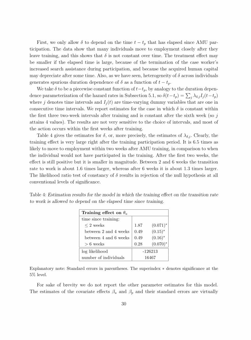
First, we only allow δ to depend on the time t − tp that has elapsed since AMU par-
ticipation. The data show that many individuals move to employment closely after they
leave training, and this shows that δ is not constant over time. The treatment effect may
be smaller if the elapsed time is large, because of the termination of the case worker’s
increased search assistance during participation, and because the acquired human capital
may depreciate after some time. Also, as we have seen, heterogeneity of δ across individuals
generates spurious duration dependence of δ as a function of t− tp.We take δ to be a piecewise constant function of t−tp, by analogy to the duration depen-
dence parameterization of the hazard rates in Subsection 5.1, so δ(t−tp) =∑
j λδ,jIj(t−tp)where j denotes time intervals and Ij(t) are time-varying dummy variables that are one in
consecutive time intervals. We report estimates for the case in which δ is constant within
the first three two-week intervals after training and is constant after the sixth week (so j
attains 4 values). The results are not very sensitive to the choice of intervals, and most of
the action occurs within the first weeks after training.
Table 4 gives the estimates for δ, or, more precisely, the estimates of λδ,j. Clearly, the
training effect is very large right after the training participation period. It is 6.5 times as
likely to move to employment within two weeks after AMU training, in comparison to when
the individual would not have participated in the training. After the first two weeks, the
effect is still positive but it is smaller in magnitude. Between 2 and 6 weeks the transition
rate to work is about 1.6 times larger, whereas after 6 weeks it is about 1.3 times larger.
The likelihood ratio test of constancy of δ results in rejection of the null hypothesis at all
conventional levels of significance.
Table 4: Estimation results for the model in which the training effect on the transition rate
to work is allowed to depend on the elapsed time since training.
Training effect on θu
time since training:≤ 2 weeks 1.87 (0.071)∗
between 2 and 4 weeks 0.49 (0.15)∗
between 4 and 6 weeks 0.49 (0.16)∗
> 6 weeks 0.28 (0.070)∗
log likelihood -126213number of individuals 16467
Explanatory note: Standard errors in parentheses. The superindex ∗ denotes significance at the5% level.
For sake of brevity we do not report the other parameter estimates for this model.
The estimates of the covariate effects βu and βp and their standard errors are virtually
30
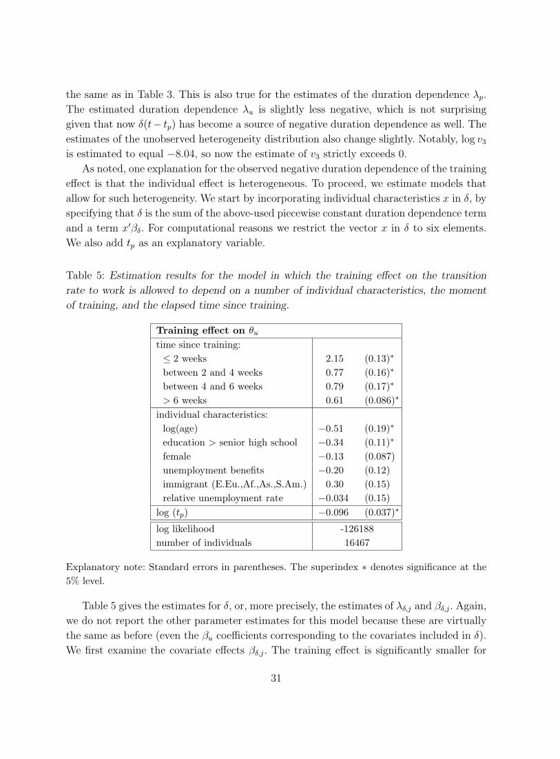
the same as in Table 3. This is also true for the estimates of the duration dependence λp.
The estimated duration dependence λu is slightly less negative, which is not surprising
given that now δ(t− tp) has become a source of negative duration dependence as well. Theestimates of the unobserved heterogeneity distribution also change slightly. Notably, log v3is estimated to equal −8.04, so now the estimate of v3 strictly exceeds 0.
As noted, one explanation for the observed negative duration dependence of the training
effect is that the individual effect is heterogeneous. To proceed, we estimate models that
allow for such heterogeneity. We start by incorporating individual characteristics x in δ, by
specifying that δ is the sum of the above-used piecewise constant duration dependence term
and a term x′βδ. For computational reasons we restrict the vector x in δ to six elements.
We also add tp as an explanatory variable.
Table 5: Estimation results for the model in which the training effect on the transition
rate to work is allowed to depend on a number of individual characteristics, the moment
of training, and the elapsed time since training.
Training effect on θu
time since training:≤ 2 weeks 2.15 (0.13)∗
between 2 and 4 weeks 0.77 (0.16)∗
between 4 and 6 weeks 0.79 (0.17)∗
> 6 weeks 0.61 (0.086)∗
individual characteristics:log(age) −0.51 (0.19)∗
education > senior high school −0.34 (0.11)∗
female −0.13 (0.087)unemployment benefits −0.20 (0.12)immigrant (E.Eu.,Af.,As.,S.Am.) 0.30 (0.15)relative unemployment rate −0.034 (0.15)
log (tp) −0.096 (0.037)∗
log likelihood -126188number of individuals 16467
Explanatory note: Standard errors in parentheses. The superindex ∗ denotes significance at the5% level.
Table 5 gives the estimates for δ, or, more precisely, the estimates of λδ,j and βδ,j. Again,
we do not report the other parameter estimates for this model because these are virtually
the same as before (even the βu coefficients corresponding to the covariates included in δ).
We first examine the covariate effects βδ,j. The training effect is significantly smaller for
31
elderly individuals, for those with a high level of education, and for those who are trained
when they are long-term unemployed. The educational effect can be explained by noting
that not many courses are available at an academic level so that individuals with a high
level of education may not be able to benefit as much from training as other individuals.
The effect of tp on the treatment effect can be due to selectivity of those who are treated
later. We return to this below.14 Also, the effect of tp may reflect an effect of t, because
of the “age-period-cohort” problem that only two of the three effects of t, tp, t − tp areidentified. The estimated effects for women and immigrants are not significantly different
from zero. The likelihood ratio test of the hypothesis that δ does not depend on observed
individual characteristics leads to rejection at all conventional levels of significance.
To compare the duration dependence coefficients in Table 5 to those in Table 4, notice
that the explanatory variables are not measured in deviation from their mean, except
for log(age), the relative unemployment rate, log tp. In addition, the average of x among
those who are exposed to training is different from the average of x in the inflow into
unemployment, because those with favorable characteristics will have found a job before
Tp is realized. For an individual with characteristics equalling the average in the inflow,
the training effect δ has estimated values 1.89, 0.51, 0.53, and 0.35 respectively as the time
since training proceeds over the four different intervals that we distinguish. The number
of 1.89 for when the time since training t− tp is less than or equal to two weeks is slightlylarger than the corresponding value in Table 4. After the initial two weeks, the treatment
effect heterogeneity in x gives rise to a dynamic selection, leading to negative duration
dependence in the effect averaged over x among the survivors. So, part of the estimated
negative duration dependence in δ in Table 4 is now captured by the heterogeneity in x.
As a result, the estimated duration dependence in Table 5 is less negative than in Table
4. In other words, not taking heterogeneity of the treatment effect into account leads to
an over-estimate of the speed at which the treatment effect vanishes after the treatment.
Nevertheless, the shape of the training effect as a function of the elapsed time since training
is qualitatively the same as before.
This line of reasoning naturally leads to the question whether the negative duration
dependence in the training effect may be due to dynamic selection because of unobserved
heterogeneity. We therefore estimate a model in which δ not only depends on t− tp and xbut also on unobserved heterogeneity. This relies on the novel identification result that we
proved in Subsection 3.2. Note that we should not include tp as a covariate in δ as it is not
clear whether such a model is identified without parametric functional form restrictions.
To keep the estimation manageable, we assume that Vδ ( and therefore log δ) is a
linear function of log Vu which is the unobserved heterogeneity term in the exit rate to
14Recall that we allow for selectivity of being treated at tp, but not yet for systematically differenttreatment effects of those with certain unobserved characteristics.
32
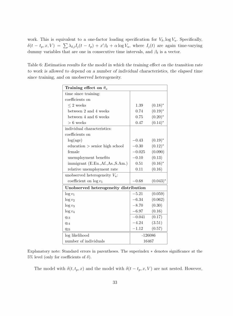
work. This is equivalent to a one-factor loading specification for Vδ, log Vu. Specifically,
δ(t − tp, x, V ) =∑λδ,jIj(t − tp) + x′βδ + α log Vu, where Ij(t) are again time-varying
dummy variables that are one in consecutive time intervals, and βδ is a vector.
Table 6: Estimation results for the model in which the training effect on the transition rate
to work is allowed to depend on a number of individual characteristics, the elapsed time
since training, and on unobserved heterogeneity.
Training effect on θu
time since training:coefficients on≤ 2 weeks 1.39 (0.18)∗
between 2 and 4 weeks 0.74 (0.19)∗
between 4 and 6 weeks 0.75 (0.20)∗
> 6 weeks 0.47 (0.14)∗
individual characteristics:coefficients onlog(age) −0.43 (0.19)∗
education > senior high school −0.30 (0.12)∗
female −0.025 (0.090)unemployment benefits −0.10 (0.13)immigrant (E.Eu.,Af.,As.,S.Am.) 0.51 (0.16)∗
relative unemployment rate 0.11 (0.16)unobserved heterogeneity Vu:coefficient on log v1 −0.68 (0.043)∗
Unobserved heterogeneity distributionlog v1 −5.21 (0.059)log v2 −6.34 (0.062)log v3 −8.70 (0.30)log v4 −6.97 (0.16)q13 −0.041 (0.17)q14 −4.24 (3.51)q23 −1.12 (0.57)
log likelihood -126086number of individuals 16467
Explanatory note: Standard errors in parentheses. The superindex ∗ denotes significance at the5% level (only for coefficients of δ).
The model with δ(t, tp, x) and the model with δ(t − tp, x, V ) are not nested. However,
33
they only differ in whether tp or v1 is included as a regressor in δ, whereas the other 71
parameters are the same. The model with v1 in δ produces a much higher likelihood value
than the other model. From this one may conclude that unobserved heterogeneity in the
treatment effect is an important feature, and, indeed, is more important than the way in
which the treatment effect depends on the moment of treatment.
The covariate effects in Table 6 are not very different from those in Table 5, except
that now immigrants have a significantly higher treatment effect than natives.15 The level
of the duration dependence coefficients in Table 6 is again difficult to compare to those in
previous tables. The unobserved heterogeneity term Vu is not included in deviation from
its mean, and, more importantly, the mean of Vu among those who are exposed to training
is lower than the mean of Vu in the inflow into unemployment. The latter is due to the
dynamic selection driven by the effect of Vu on the exit rate to work before the treatment
is realized.
The observed and unobserved heterogeneity in the determinants of the treatment effect
give rise to a large amount of heterogeneity of the treatment effect itself across individuals.
For individuals with Vu = v1, the treatment effect on the exit rate to work is so large
that virtually all of them will leave unemployment within some weeks after training. Of
course, with Vu having a high value, the exit rate to work is relatively high, so that many
would move to work before Tp is realized. Also, among those for whom Vu is large, the
probability that Vp is large is very small (in the inflow it is 1.4%, which follows from
Pr(Vu = v1, Vp = v3) = 0.417 and Pr(Vu = v1, Vp = v4) = 0.006), so their treatment rate is
very small. In sum, very few v1-individuals will be exposed to the treatment. Note that in
reality, for given x, there are most likely more than two types of individuals, and it is not
clear for how many of them the estimated value of v1 is appropriate.
Let us return to the duration dependence shape of the treatment effect. The treatment
effect heterogeneity in V gives rise to an additional dynamic selection, leading to negative
duration dependence in the treatment effect averaged over V among the survivors. As
follows from the previous paragraph, in our estimated model this issue is primarily relevant
in the very first weeks after training. It implies that part of the estimated negative duration
dependence in δ in Table 5 is now explained by the heterogeneity in V . As a result, the
estimated duration dependence in Table 6 is less negative than in Table 5. In other words,
not taking unobserved heterogeneity of the treatment effect into account leads to an over-
estimate of the speed at which the treatment effect vanishes after the treatment.
Nevertheless, for many individuals the shape of the training effect as a function of the
elapsed time since training is qualitatively similar to before. For many individuals, the exit
rate to work in the first two weeks after training is more than 3 times larger than the
counterfactual exit rate in the absence of training. Also, the individual exit rate to work
15In Table 5 the t-value is 1.95.
34
in the seventh week after training is only 40% (=exp(0.47− 1.39)) of the exit rate duringthe first two weeks after training.
Consider for example a native male individual, aged 36, with a high-school education
level, who receives unemployment insurance, lives in a region with average labor market
conditions, and has Vu = v2. His exit rate to work in the first two weeks after training is
3.6 times larger than in the absence of training, and his exit rate to work in the seventh
week after training is only 1.4 times larger than in the absence of training. For an otherwise
equal woman, these numbers are virtually the same (3.5 and 1.4). If they would have age
55 instead of 36 then these numbers are 3.0 and 1.2. If the individual is an immigrant
and/or aged in their twenties then the effects are larger, while if he/she is highly educated
then they are smaller. Notice that for identification reasons we do not allow for interaction
effects between covariates and the time since training.
5.4 Interpretation of the treatment-effect estimates
Recall that the official purpose of AMU is to increase the transition rate to work, and that
this is supposed to be achieved by way of skill enhancements, i.e. by way of productivity
improvements. Human capital accumulation by itself cannot explain the peak in the indi-
vidual exit rate to work right after training. After all, skills do not depreciate at the rate
at which the training effect decreases. The same applies to signaling-and-screening effects
of having completed training. It is also difficult to explain the peak by the accumulation of
vacancies or job offers during the period of training: it is hard to imagine that an employer
is willing to reserve a vacancy for an individual who may or may not be available 3 or 6
months later (and who may by then have accumulated the appropriate skills).
It is therefore likely that the peak is driven by the increased job-search assistance
efforts by the case workers towards the end of the training period. These efforts make it
easier for employers to find suitable workers. After the training is completed, the job-search
assistance efforts return to their normal level. This explains why the treatment effect does
not stay at a high level as the elapsed time since training increases.
In our estimates, the effect on the exit rate to work does not vanish as time proceeds.
Six weeks after the training, the exit rate is often still 40% higher than in the absence of
training, which is substantial. Of course it remains to be seen whether this magnitude is
persistent in case of model general model specifications. Presumably, the resulting estimates
for the long-run effect will be smaller than 40% if we allow for a larger number of time
intervals in the piecewise-constant duration-dependence of the effect, and/or more possible
realizations of unobserved heterogeneity in the effect, and/or a non-deterministic relation
between Vδ and Vu, and/or observed course heterogeneity, and/or interactions between
covariates and duration dependence in the effect. (The computational demands would
35
however increase dramatically.) The fact that other studies have consistently failed to find
AMU effects on income supports the hypothesis that the productivity-enhancement effect
is small. This is in line with a treatment effect on the exit rate to work that converges in
the long run to a small number.
If the success of the job search assistance efforts right after training is due to a pro-
ductivity improvement of the worker, then the total training effect can be increased by
extending the job search assistance efforts in time. If the success of the job search as-
sistance efforts is simply due to bridging the search-frictions information gap, then the
training courses are not needed in the first place. In either case, it seems that the over-all
effect can be improved if resources are reallocated away from the training courses towards
job search assistance. Also, in the light of the amount of heterogeneity in the training effect,
it seems that AMU can be made more effective by a stronger pre-screening and selection
of potential candidates on their characteristics.
5.5 Time in training
We now incorporate the time spent in AMU training into the duration analysis, that is,
we drop the rule that the length of the time interval spent within AMU training is set
to zero. There are two major issues involved. First, the time in training adds to the time
out of work. This is the so-called lock-in effect of training. Treatment effects on the total
time out of work should incorporate this. This can be carried out in a straightforward way
with the results of the previous subsections, by carefully adding the time in training to the
duration out of work for someone who has been in training, when calculating effects on the
mean duration out of work.
The second issue is that individuals may influence the time they are in training. In the
data, the time in training is not constant across spells with training. To a large extent
this reflects course heterogeneity. It is not known whether course heterogeneity gives rise
to selectivity in course enrolment, and also not whether the moment at which training
ends is driven by selective drop-out behavior. It is difficult deal with such selection effects.
Relatively short times in training are rarely observed, so perhaps selective drop-out is not
a major concern.
Incorporating the time in training into the duration model may lead to different esti-
mated effects on the exit rate to work. Consider for example the training effect directly
after leaving training. Let t0 be the duration at entry into training. So far, the effect has
been obtained by comparing (a) the exit rate of individuals who complete training, eval-
uated at the moment they complete training, to (b) the exit rate of individuals who have
not entered training at t0, evaluated at t0, while appropriately taking selection effects into
account. With a positive time in training, one may argue that (b) should be replaced by
36

a measure that reflects the exit rate of non-trained individuals evaluated at t0 plus the
training time. After all, the duration dependence in the exit rate to work may be driven
by the time out of work rather than the time in open unemployment.
From the previous two paragraphs it follows that models incorporating the time in
training would be complex, and we feel that the empirical analysis of such models is
beyond the scope of the paper. Instead we provide estimates of treatment effects on the
time out of work based on results from the previous subsections, and we provide estimates
of relatively simple duration models to shed some further light on the size of the lock-in
effect. It should be borne in mind that all these results do not take account of course-length
selection effects or drop-out selection effects.
Let us now discuss the duration analyses. Consider the basic model estimated in Sub-
section 5.2, where we now let δ depend on whether the total time in training was short
(smaller than 90 days) or long. If, as before, we stop the time clock during training, so
that the duration variable does not take account of the time in training, then we obtain
that δ is estimated by 0.67 for short courses (standard error 0.066) and by 0.76 for long
courses (standard error 0.064). This suggests that long courses are slightly beneficial in
their effect on the exit rate to work. Now suppose that we let the time clock run during
training, and we let the treatment effect δ affect the exit rate to work from the onset of
training, where δ only depends on whether the course is short or long. Clearly, this ig-
nores that in reality the exit rate to work is very small during training and is large after
training. The parameter estimate will capture some average of the low exit rate to work
during training and the training effect after leaving training. Consequently, we expect the
estimate of δ to be smaller than in Table 3. Indeed, we obtain that δ is estimated by
0.24 for short courses (standard error 0.069) and by –0.35 for long courses (standard error
0.084). What this shows is that the over-all training effect that comprises the lock-in effect
and the post-training effect together is very small. As seen from the moment at which the
individual enters training, the lock-in effect is of a similar order of magnitude, but with
an opposite sign, as the post-training effect on the exit rate to work. This is due to the
fact that individuals do not often move from training to work during the first five months
of AMU training. Note that this explanation is consistent with the fact that the over-all
effect is more negative for long courses than for short courses, After all, the longer courses
have a substantially larger lock-in effect but only a marginally larger post-training effect.
The fact that the other parameter estimates are similar to before means that they are
insensitive to whether we include time spent in other programs or not.
37

5.6 Participation in other programs
The present paper does not aim to analyze the effects of participation in other active labor
market programs, neither in isolation from AMU training, nor in possible interaction with
AMU training and its effects. We have already seen that AMU training is regarded as being
fundamentally different from other programs, and substitution seems to be absent. The
data suggest that AMU training and other programs are unrelated activities. Nevertheless,
the way we handle the actual time spent in other programs may affect our estimate of
the training effect on the exit rate to work. To shed some more light on this we estimate
a model version in which time spent in other programs not ignored but is added to time
in unemployment. For Tu this is appropriate if individuals move to employment at the
same rate within other programs as they do when they are openly unemployed. For Tp
this is appropriate if individuals move into AMU at the same rate when they are in other
programs as they do when they are openly unemployed. The estimate of δ in the basic
model now equals 0.54 (standard error 0.052), which is slightly lower than in Table 3. It
was to be expected that the estimate would be somewhat lower, because now the treated
are effectively compared to not-yet treated who are at an earlier stage of the unemployment
spell than the comparison group used earlier.
The fact that the other parameter estimates are similar to before means that they
are insensitive to whether we include time spent in other programs or not. The duration
dependence of the inflow rate into AMU is more negative than before. This reflects the fact
that individuals cannot be in AMU training and in another program at the same time.
We can combine our current approach to that of the previous subsection, meaning that
we let the time clock run during training and other program participation, and we let
the training effect δ affect the exit rate to work from the onset of training, where δ only
depends on whether the training course is short or long. This gives an estimate for δ of
0.18 for short courses (standard error 0.067) and of –0.26 for long courses (standard error
0.081). So, the over-all training effect on the total time out of work is even closer to zero
if we take time in other programs into account.
Finally, we return to the framework of Subsection 5.3 where the clock is halted during
program participation and the treatment effect is heterogeneous. We estimate a model in
which the effect is also allowed to depend on a dummy variable indicating whether the
individual has participated in another program during the current spell of unemployment
before entry into training. The corresponding parameter estimate equals 0.17 (standard
error 0.068). This suggests that the effect of AMU training benefits from an earlier partic-
ipation in another program. Recall however that we do not control for selectivity of such
program participation.
38
6 Conclusions
The individual transition rate from unemployment to employment is significantly and sub-
stantially raised as a result of the individual’s participation in an AMU vocational training
course. Individual re-employment rates are more or less tripled upon completion of the
AMU course. However, this large effect only holds during the first few weeks after comple-
tion of the course. This may reflect the fact that caseworkers provide extra effort to find a
job for AMU participants towards the end of the course. The observed decline of the effect
can only to a limited degree be explained by dynamic weeding out due to heterogeneity of
individuals’ skills and other characteristics. When we take the time spent within the pro-
gram into account as well, then the net effect on the individual’s unemployment duration
is about zero. Thus, the program does not appear to be cost-effective.
It seems that the over-all effect can be improved if resources are reallocated away
from the training course, in the sense that their durations are shortened, towards a more
prolonged job search assistance effort by the case worker after completion of the course.
Also, in the light of the amount of heterogeneity in the training effect, it seems that AMU
can be made more effective by a stronger pre-screening and selection of potential candidates
on their characteristics.
There are some topics for further research. We have argued that the empirical analysis
has benefited from the availability of multi-spell data. In fact, any stochastic dependence
across spells of the same individual can only be due to the presence of heterogeneity. It is
ruled out by assumption that realizations of the unemployment duration or the training
program in one spell affect the distributions of these in another spell. This may be a
strong assumption. A topic for future work would be to examine to what extent AMU
courses have effects that carry over to future unemployment spells (although the finding
that the effect is strongest right after completion of the course suggests that such long-
term effects may be negligible). Another topic for further research is to add hourly wages
as an outcome variable. Comprehensive Swedish register information on hourly wages is
expected to become widely available in the near future.
39
Appendix. Proof of Proposition 1
Suppose first that the distribution of the observed explanatory variables X is degenerate.
As in Abbring and Van den Berg (2003), the information in a large data set can then be
summarized by
Qp(t, tp) := Pr(Tu > t, Tp > tp, Tu > Tp) and Qu(t) := Pr(Tu > t, Tu < Tp) (5)
for all (t, tp) ∈ R2+. These are the so-called sub-survival-functions of (Tu, Tp) and Tu for the
sub-populations with Tu > Tp and Tu < Tp, respectively.
Note that the distribution of the identified minimum of (Tu, Tp), i.e. the smallest of
Tu and Tp, together with the identity of this smallest duration, is fully characterized by
(Q0p, Qu), with Q
0p(tp) := Qp(−∞, tp) for all tp ∈ R+.
Now let X be allowed to be heterogeneous. In obvious notation, the data then come in
the form of a collection {Qp, Qu} := {(Qp(·|x), Qu(·|x));x ∈ X} of conditional sub-survivalfunctions. Here, X ⊂ R
k, 1 ≤ k <∞, is the support of X.We adopt the model of Subsection 3.2. In fact, we consider a slightly more general
model where exp(x′βi) is replaced by φi(x),
θp(t|x, Vp) = λp(t) · φp(x) · Vp
θu(t|tp, x, Vu, Vδ) = λu(t) · φu(x) · Vu · exp(δ(t− tp, x, Vδ) · I(t > tp))δ(t− tp, x, Vδ) = λδ(t− tp) + φδ(x) + Vδ
Notice that λu(.), φu(.) and Vu act multiplicatively on θu(t|tp, x, Vu, Vδ) while at the same
time exp(λδ(.)), exp(φδ(.)) and exp(Vδ) act multiplicatively on θu(t|tp, x, Vu, Vδ). This asym-
metry between notation indexed by u and p on the one hand and notation indexed by δ
on the other hand complicates some expressions below.
We make the following regularity conditions, assumptions, and normalizations.
Assumption 1. Variation over observed covariates.
φu, φp, and φδ are continuous functions φp : X → (0,∞) and φu : X → (0,∞) andφδ : X → (−∞,∞). Further, {(φu(x), φp(x));x ∈ X} contains a non-empty open set in R
2
and {φu(x) · exp(φδ(x));x ∈ X} contains a non-empty open interval in R.
Assumption 2. Baseline hazards.
The functions λu : R+ → (0,∞) and λp : R+ → (0,∞) are continuous except at at most afinite number of known points. They have integrals
Λu(t) :=
∫ t
0
λu(τ)dτ <∞ and Λp(t) :=
∫ t
0
λp(τ)dτ <∞
40

for all t ∈ R+. The function λδ : R+ → (−∞,∞) is continuous except at at most a finitenumber of known points. Moreover, its integral
Λ∆(t) :=
∫ t
0
exp(λδ(τ))dτ
exists and is finite for all t ∈ R+. The functions λδ and λu are such that
K(t, tp) :=
∫ t
tp
λu(τ) exp(λδ(τ − tp))dτ
exists and is finite for all {(t, tp) ∈ R2 : t > tp ≥ 0}.
Assumption 3. Independence of observed and unobserved heterogeneity.
(Vu, Vp, Vδ) is independent of X.
Assumption 4. Positive unobserved heterogeneity.
Pr((Vu, Vp, exp(Vδ)) ∈ (0,∞)3) = 1.Assumption 5. Finite means of unobserved heterogeneity.
E[Vu] <∞ and E[Vp] <∞ and E[VuVp exp(Vδ)] <∞.Assumption 6. Normalizations.
For some a priori chosen x∗ ∈ X , there holds that φu(x∗) = φp(x
∗) = 1 and φδ(x∗) = 0.
For some a priori chosen t∗ ∈ (0,∞), Λu(t∗) = Λp(t
∗) = K(t∗, 0) = 1.
We now introduce some new notation. Let λ∆, φ∆, and V∆ be defined such that for every
t, x, Vu, Vδ,
V∆ = Vu exp(Vδ),
λ∆(t) = exp(λδ(t))
φ∆(x) = φu(x) exp(φδ(x))
Consequently, the exit rate to work at t > tp can be expressed as
θ(t|tp, x, V∆) = λu(t)φ∆(x)λ∆(t− tp)V∆
By Proposition 2 in Abbring and Van den Berg (2003), the functions Λu,Λp, φu and φp
and the joint distribution of Vu, Vp are identified from {Q0p, Qu}, given the assumptions
listed above. We proceed by subsequently identifying the functions Λ∆ and φ∆ and the
joint distribution of Vu, V∆, Vp from Qp. Once we established this, the identification of
41
the functions Λδ and φδ and the joint distribution of Vu, Vp, Vδ follows immediately. The
structure of the remainder of the proof is similar to the structure of the proof in Abbring and
Van den Berg (2003) of identification of a model where δ depends on x, t, and unobserved
heterogeneity V (their Proposition 4).
Let L denote the trivariate Laplace transform of the distribution G∆ of (Vu, V∆, Vp),
and L(∆p)(z1, z2, z3) := ∂2L(z1, z2, z3)/∂z2∂z3 for all (z1, z2, z3) ∈ (0,∞)3. Note that As-
sumption 3 implies that (Vu, Vp, V∆)⊥⊥X.For fixed x ∈ X , ∂2Qp(t, tp|x)/∂t∂tp and ∂2Qp(t, tp|x∗)/∂t∂tp exist for almost all t, tp ∈
R+ such that tp < t. For these (t, tp),
∂2Qp(t, tp|x)/∂t∂tp∂2Qp(t, tp|x∗)∂t∂tp = φp(x)φ∆(x)
L(∆p)(φu(x)Λu(tp), φ∆(x)K(t, tp), φp(x)Λp(tp))
L(∆p)(Λu(tp), K(t, tp),Λp(tp))(6)
If t ↓ 0 and tp ↓ 0, both sides of (6) above reduce to φp(x)φ∆(x) because, by assumption,
E[V∆Vp] = limz↓(0,0,0) L(∆S)(z) < ∞. We have already identified φp, and the left-hand side
is data, so this identifies φ∆.
For arbitrary x ∈ X and t, tp ∈ R+ such that tp < t there also holds that
∂Qp(t, tp|x)/∂tpλp(tp)φp(x)
= L(p)(φu(x)Λu(tp), φ∆(x)K(t, tp), φp(x)Λp(tp)), (7)
with L(p)(z1, z2, z3) := ∂L(z1, z2, z3)/∂z3. Note that the left-hand side of this equation isalready identified for all tp arbitrarily close to zero. As tp ↓ 0, the right-hand side reducesto
L(p)(0, φ∆(x)K(t, 0), 0). (8)
After imposing t = t∗, we can identify the completely monotone function −L(p)(0, ·, 0)on a nonempty open set in R by appropriately varying x in equation (8). This identifies
−L(p)(0, z, 0) for all z ∈ (0,∞) because of the real analyticity of −L(p)(0, ·, 0) (see below).Subsequently, the right-hand side of (8) is strictly monotone in K, so K(t, 0) can be traced
out by varying t, and as a result the function K(t, 0) as a function of t is identified. Recall
that K(t, 0) =∫ t
0λu(τ)λ∆(τ)dτ . Given Assumption 2, this suffices to identify Λ∆(t) for all
t > 0.
Finally, by appropriately varying x and t in equation (7), we can trace L(p) on an
nonempty open subset of R3. This identifies L(p) on (0,∞)3 because −L(p) is real analytic.
This in turn identifies L (see Abbring and Van den Berg, 2006).
42

References
Abbring, J.H. and G.J. van den Berg (2003), “The non-parametric identification of treat-
ment effects in duration models”, Econometrica, 71, 1491–1517.
Abbring, J.H. and G.J. van den Berg (2004), “Analyzing the effect of dynamically assigned
treatments using duration models, binary treatment models, and panel data models”,
Empirical Economics, 29, 5–20.
Abbring, J.H. and G.J. van den Berg (2005), “Social experiments and instrumental vari-
ables with duration outcomes”, Working paper, Free University Amsterdam, Amster-
dam.
Abbring, J.H. and G.J. van den Berg (2006), “Corrigendum on the non-parametric identi-
fication of treatment effects in duration models”, Working paper, Free University Ams-
terdam, Amsterdam.
AMS (1997), “Employment training”, Working paper, AMS, Solna.
AMS (1998), “Labour market policy programmes”, Working paper, AMS, Solna.
AMS (2001), “Yearly report on labour market policy programmes”, Working paper, AMS,
Solna (in Swedish).
Bjorklund, A. (1993), “The Swedish experience”, in Measuring labour market measures,
Ministry of Labour, Denmark, Copenhagen.
Brannas, K. (2000), “Estimation in a duration model for evaluating educational programs”,
Working paper, Umea University, Umea.
Carling, K., P.A. Edin, A. Harkman, and B. Holmlund (1996), “Unemployment duration,
unemployment benefits and labor market programs in Sweden”, Journal of Public Eco-
nomics, 59, 313–334.
Carling, K., B. Holmlund, and A. Vejsiu (2001), “Do benefit cuts boost job findings?
Swedish evidence from the 1990s”, Economic Journal, 111, 766–790.
Carling, K. and K. Richardson (2004), “The relative efficiency of labor market programs:
Swedish experience from the 1990’s”, Labour Economics, 11, 335–354.
Dahlberg, M. and A. Forslund (2005), “Direct displacement effects of labour market pro-
grammes”, Scandinavian Journal of Economics, 107, 475–494.
Edin, P.A., A. Harkman, B. Holmlund, and H. Soderberg (1998), “Escaping long-term
unemployment in Sweden”, Working paper, Uppsala University, Uppsala.
Edin, P.A. and B. Holmlund (1991), “Unemployment, vacancies and labour market pro-
grammes: Swedish evidence”, in F. Padoa Schioppa, editor, Mismatch and Labour Mo-
bility, Cambridge University Press, Cambridge.
43
Eriksson, M. (1997a), “Comparison of compensatory and non-compensatory models for
selection into labour market training”, Working paper, Umea University, Umea.
Eriksson, M. (1997b), “Placement of unemployed into labour market programs: a quasi-
experimental study”, Working paper, Umea University, Umea.
Fay, R.G. (1996), “Enhancing the effectiveness of active labour market policies: Evidence
from programme evaluations in OECD countries”, Working paper, OECD, Paris.
Harkman, A. and A. Johansson (1999), “Training or subsidized jobs – what works?”,
Working paper, AMS, Solna.
Heckman, J.J., R.J. LaLonde, and J.A. Smith (1999), “The economics and econometrics
of active labor market programs”, in O. Ashenfelter and D. Card, editors, Handbook of
Labor Economics, Volume III, North-Holland, Amsterdam.
Heckman, J.J. and C.R. Taber (1994), “Econometric mixture models and more general
models for unobservables in duration analysis”, Statistical Methods in Medical Research,
3, 279–302.
Honore, B.E. (1991), “Identification results for duration models with multiple spells or
time-varying covariates”, Working paper, Northwestern University, Evanston.
Lancaster, T. (1990), The Econometric Analysis of Transition Data, Cambridge University
Press, Cambridge.
Larsson, L. (2003), “Evaluation of Swedish youth labour market programmes”, Journal of
Human Resources, 38, 891–927.
Regner, H. (1997), “Training at the job and training for a new job: two Swedish studies”,
Working paper, SOFI, Stockholm.
Regner, H. (2002), “A nonexperimental evaluation of training programs for the unemployed
in Sweden”, Labour Economics, 9, 187–206.
Ridder, G. (1990), “The non-parametric identification of generalized accelerated failure-
time models”, Review of Economic Studies, 57, 167–182.
Van den Berg, G.J. (2001), “Duration models: Specification, identification, and multiple
durations”, in J.J. Heckman and E. Leamer, editors, Handbook of Econometrics, Volume
V, North Holland, Amsterdam.
44