SWAT model calibration of a grid-based setup

Adv. Geosci., 32, 55–61, 2012www.adv-geosci.net/32/55/2012/doi:10.5194/adgeo-32-55-2012© Author(s) 2012. CC Attribution 3.0 License.

Advances inGeosciences

SWAT model calibration of a grid-based setup

H. Rathjens and N. Oppelt

Kiel University, Department of Geography, Ludewig-Meyn-Str. 14, 24098 Kiel, Germany

Correspondence to:H. Rathjens ([email protected])

Received: 31 January 2012 – Revised: 12 June 2012 – Accepted: 4 November 2012 – Published: 11 December 2012

Abstract. The eco-hydrological model SWAT (Soil and Wa-ter Assessment Tool) is a useful tool to simulate the effectsof catchment processes and water management practices onthe water cycle. For each catchment some model parameters(e.g. ground water delay time, ground water level) remainconstant and therefore are used as constant values; other pa-rameters such as soil types or land use are spatially variableand thus have to be spatially discretized. SWAT setup inter-faces process input data to fit the data format requirementsand to discretize the spatial characteristics of the catchmentarea. The primarily used configuration is the sub-watersheddiscretization scheme. This spatial setup method, however,results in a loss of spatial information which can be problem-atic for SWAT applications that require a spatially detaileddescription of the catchment area. At present no SWAT inter-face is available which provides the management of input andoutput data based on grid cells. To fill this gap, the authorsdeveloped a grid-based model interface.

To perform hydrological studies, the SWAT user first cali-brates the model to fit to the environmental and hydrologicalconditions of the catchment. Compared to the sub-watershedapproach, the grid-based setup significantly increases modelcomputation time and hence aggravates calibration accordingto established calibration guidelines. This paper describeshow a conventional set of sub-watershed SWAT parameterscan be used to calibrate the corresponding grid-based model.The procedure was evaluated in a sub-catchment of the RiverElbe (Northern Germany). The simulation of daily dischargeresulted in Nash-Sutcliffe efficiencies ranging from 0.76 to0.78 and from 0.61 to 0.65 for the calibration and validationperiod respectively; thus model performance is satisfactory.The sub-watershed and grid configuration simulate compa-rable discharges at the catchment outlet (R2

= 0.99). Never-theless, the major advantage of the grid-based set-up is an en-hanced spatial description of landscape units inducing a morerealistic spatial distribution of model output parameters.

1 Introduction

The eco-hydrological model SWAT (Soil and Water Assess-ment Tool,Arnold et al., 1998) is a useful tool for a widerange of scales and environmental conditions. In literaturemanifold SWAT applications have been reported; the topicscover hydrological and water resource assessments (waterdischarge, groundwater dynamics, soil water, snow dynam-ics, water management), water quality assessments (land-useand land-management change in agriculture), climate changeimpacts, and pollutant assessments (Gassman et al., 2007); adetailed review can be found inGassman et al.(2007) andKrysanova and Arnold(2008).

To set up a SWAT model run, the watershed has to be de-lineated and the spatial arrangement of catchment elements(e.g. sub-catchments, reach segments and point sources) hasto be defined (Neitsch et al., 2011a). The most popularsetup is the sub-watershed configuration, where the catch-ment is divided into sub-catchments and further sub-dividedinto hydrologic response units (HRUs). The HRUs repre-sent percentages of the sub-catchment area (Gassman et al.,2007). Individual areas of similar soil, topography and land-use are lumped together within a sub-catchment to form anHRU while in reality they are scattered throughout the sub-catchment. Thus this approach fails to show the interactionbetween the HRUs as they are spatially unlinked but routedto the outlet of the sub-catchment separately (Arnold et al.,2010).

The grid-based setup within SWAT overcomes the diffi-culties of the sub-watershed configuration (Rathjens and Op-pelt, 2012). The user is able both to refine the spatial reso-lution of a SWAT model and to obtain spatially distributedmodel output data. Various GIS (Geographic InformationSystem) applications can process the grid-based output; nowthe model output of every grid cell with its defined geograph-ical position can be analysed. Due to the open-source sta-tus of the SWAT code the grid-based approach will continue

Published by Copernicus Publications on behalf of the European Geosciences Union.

56 H. Rathjens and N. Oppelt: SWAT model calibration of a grid-based setup

to evolve as users determine needed improvements, which isan advantage in comparison to other catchment scale raster-based models such as MIKE-SHE (Refsgaard and Storm,1995), TOPMODEL (Beven and Kirkby, 1979) or WASIM(Schulla, 1997). The grid based approach, however, signifi-cantly increases computation time.Arnold et al.(2010) statedthat, applying a one-hectare grid cell size (approx. 50 000 000grid cells) to the the Upper Mississippi River basin, the sim-ulation of a single year would require about 13 computationdays on a 2.6 GHz processor.

After processing of the input data, model calibration isperformed, i.e. model output and in-situ data are comparedto improve model input parameters iteratively. According toNeitsch et al.(2011a) the calibration of stream flow is per-formed in two consecutive steps. The model is calibratedfor average annual conditions first; then the user shifts tomonthly or daily records to fine-tune the calibration. To ob-tain sufficient calibration results several model runs mightbe performed. Model validation follows calibration; the in-put parameters, which were derived during calibration, noware used to test the resulting model performance for a seriesof subsequent years (Moriasi et al., 2007). Most applicationsuse the discharge at the catchment outlet to calibrate and val-idate model performance.

For the grid-based model setup, however, this time-consuming procedure is impractical. Therefore, this paperprovides a method for grid-based SWAT setups to calibratedaily discharge at the catchment outlet. To perform this anal-ysis, calibration parameters are derived with a sub-watershedconfiguration and then transferred to a grid-based model. TheGIS interface ArcSWAT (Winchell et al., 2010) is used togenerate the input files for the conventional sub-watershedsetup; SWATgrid (Rathjens and Oppelt, 2012) is used tosetup the grid cell model. A sub-catchment of the River Elbe,the Bunzau catchment, serves as test site to present and vali-date the proposed methodology.

2 Materials and methods

2.1 Study area

The Bunzau catchment is located in the Northern Germanlowlands (see Fig.1); it covers an area of 210 km2 and ischaracterized by flat topography and shallow groundwaterlevels. The mean annual precipitation is 857 mm and themean annual temperature is 9.51◦C (stations Neumunsterand Padenstedt, 2000–2009) (DWD, 2011). The RiversBuckener Au and Fuhlenau merge north of Aukrug-Innienand form the origin of the River Bunzau; the Rivers Hollenauand Bredenbek form two downstream tributaries. Severaldrainage pipes and ditches also flow into the Bunzau, whichflows in southern direction for 16 km before it flows intothe Stor River. The gauge Sarlhusen is located close to the

Fig. 1.The Bunzau catchment and its location in Germany.

catchment outlet, where an average discharge of 2.51 m3 s−1

was measured between 2000 and 2009.In the Bunzau catchment dominant soils types are pod-

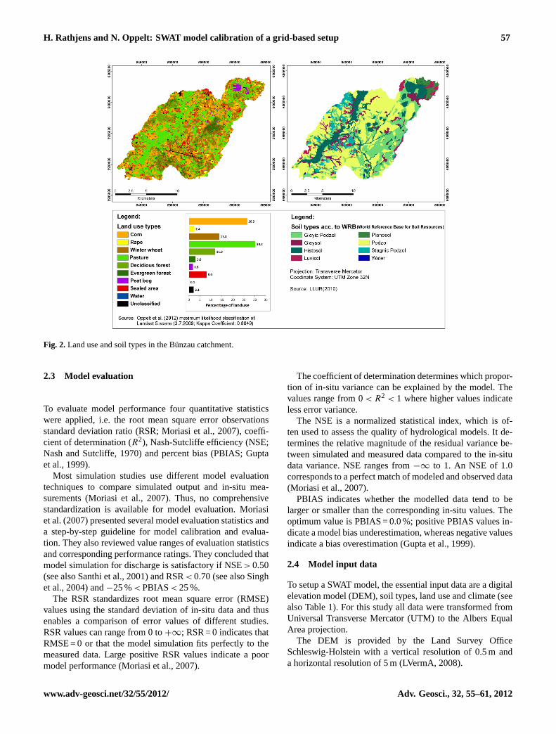
zols and planosols; histosols are found in river valleys anddepressions. High proportions of arable land (43 %) and pas-ture (30 %) indicate an intense agricultural use; Fig.2 showsthe land use in 2009 as well as the distribution of soil types.

2.2 The SWAT model

SWAT (Arnold et al., 1998) is a physically based catchment-scale model; it was developed to simulate the water cycle, thecorresponding fluxes of energy and matter (e.g. sediment, nu-trients, pesticides and bacteria) as well as the impact of man-agement practices on these fluxes. The design of the modelis modular and includes components for hydrology, weather,sedimentation, crop growth, nutrients and agricultural man-agement. A detailed description of all components can befound inArnold et al.(1998) andNeitsch et al.(2011b).

The simulated hydrological processes include surfacerunoff (SCS (Soil Conservation Services) curve number orGreen and Ampt infiltration equation), percolation, lateralflow, groundwater flow from shallow aquifers to streams,evapotranspiration (Hargreaves, Priestley-Taylor or Penman-Monteith method), snowmelt, transmission losses fromstreams and water storage and losses from ponds (Arnoldet al., 1998).

In this study the SCS curve number method (Soil Conser-vation Service Engineering Division, 1972) was used to cal-culate surface runoff; Penman-Monteith method was appliedto estimate potential evapotranspiration.

Adv. Geosci., 32, 55–61, 2012 www.adv-geosci.net/32/55/2012/

H. Rathjens and N. Oppelt: SWAT model calibration of a grid-based setup 57

Fig. 2.Land use and soil types in the Bunzau catchment.

2.3 Model evaluation

To evaluate model performance four quantitative statisticswere applied, i.e. the root mean square error observationsstandard deviation ratio (RSR;Moriasi et al., 2007), coeffi-cient of determination (R2), Nash-Sutcliffe efficiency (NSE;Nash and Sutcliffe, 1970) and percent bias (PBIAS;Guptaet al., 1999).

Most simulation studies use different model evaluationtechniques to compare simulated output and in-situ mea-surements (Moriasi et al., 2007). Thus, no comprehensivestandardization is available for model evaluation.Moriasiet al.(2007) presented several model evaluation statistics anda step-by-step guideline for model calibration and evalua-tion. They also reviewed value ranges of evaluation statisticsand corresponding performance ratings. They concluded thatmodel simulation for discharge is satisfactory if NSE> 0.50(see alsoSanthi et al., 2001) and RSR< 0.70 (see alsoSinghet al., 2004) and−25 %< PBIAS< 25 %.

The RSR standardizes root mean square error (RMSE)values using the standard deviation of in-situ data and thusenables a comparison of error values of different studies.RSR values can range from 0 to+∞; RSR = 0 indicates thatRMSE = 0 or that the model simulation fits perfectly to themeasured data. Large positive RSR values indicate a poormodel performance (Moriasi et al., 2007).

The coefficient of determination determines which propor-tion of in-situ variance can be explained by the model. Thevalues range from 0< R2 < 1 where higher values indicateless error variance.

The NSE is a normalized statistical index, which is of-ten used to assess the quality of hydrological models. It de-termines the relative magnitude of the residual variance be-tween simulated and measured data compared to the in-situdata variance. NSE ranges from−∞ to 1. An NSE of 1.0corresponds to a perfect match of modeled and observed data(Moriasi et al., 2007).

PBIAS indicates whether the modelled data tend to belarger or smaller than the corresponding in-situ values. Theoptimum value is PBIAS = 0.0 %; positive PBIAS values in-dicate a model bias underestimation, whereas negative valuesindicate a bias overestimation (Gupta et al., 1999).

2.4 Model input data

To setup a SWAT model, the essential input data are a digitalelevation model (DEM), soil types, land use and climate (seealso Table1). For this study all data were transformed fromUniversal Transverse Mercator (UTM) to the Albers EqualArea projection.

The DEM is provided by the Land Survey OfficeSchleswig-Holstein with a vertical resolution of 0.5 m anda horizontal resolution of 5 m (LVermA, 2008).

www.adv-geosci.net/32/55/2012/ Adv. Geosci., 32, 55–61, 2012


Table 1.Model input data sources.

Data type Source Data description and properties

Topography (DEM) LVermA (2008) Digital elevation model, 5 m× 5 m resolutionSoil map Finnern(1997) Physical properties of the soil (e.g. available water capacity), scale 1 : 100 000

LLUR (2010) Physical properties of the soil (e.g. available water capacity), scale 1 : 25 000Land use map 2009 Oppelt et al.(2012) Classifications based on Landsat 5 imagery (3 July 2009), 30 m× 30 m resolutionClimate data DWD (2011) Daily measured values of temperature, precipitation, wind speed, relative humidity

(Neumunster station 2000–2007, Padenstedt station 2007–2009)Daily measured values of precipitation (Gnutz station 2000–2006)

Discharge LKN (2011) Daily discharge data of the Bunzau river at gauge Sarlhusen (2000–2009)

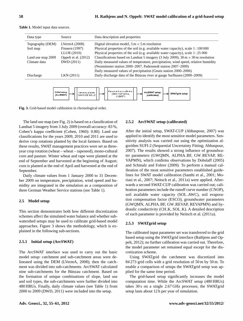
Fig. 3.Grid-based model calibration in chronological order.

The land use map (see Fig.2) is based on a classification ofLandsat 5 imagery from 3 July 2009 (overall-accuracy: 83 %,Cohen’s kappa coefficient (Cohen, 1960): 0.80). Land useclassifications for the years 2009, 2010 and 2011 are used toderive crop rotations planted by the local farmers. Based onthese results, SWAT management practices were set as three-year crop rotation (wheat – wheat – rapeseed), mono-culturalcorn and pasture. Winter wheat and rape were planted at theend of September and harvested at the beginning of August;corn is planted at the end of April and harvested at the end ofSeptember.

Daily climate values from 1 January 2000 to 31 Decem-ber 2009 on temperature, precipitation, wind speed and hu-midity are integrated in the simulation as a composition ofthree German Weather Service stations (see Table1).

2.5 Model setup

This section demonstrates both how different discretizationschemes affect the simulated water balance and whether sub-watershed setups may be used to calibrate grid-based modelapproaches. Figure3 shows the methodology, which is ex-plained in the following sub-sections.

2.5.1 Initial setup (ArcSWAT)

The ArcSWAT interface was used to carry out the basicmodel setup: catchment and sub-catchment areas were de-lineated using the DEM (LVermA, 2008); then the catch-ment was divided into sub-catchments. ArcSWAT calculatednine sub-catchments for the Bunzau catchment. Based onthe formation of unique combinations of slope, land useand soil types, the sub-catchments were further divided into480 HRUs. Finally, daily climate values (see Table1) from2000 to 2009 (DWD, 2011) were included into the setup.

2.5.2 ArcSWAT setup (calibrated)

After the initial setup, SWAT-CUP (Abbaspour, 2007) wasapplied to identify the most sensitive model parameters. Sen-sitivity analysis was carried out using the optimization al-gorithm SUFI-2 (Sequential Uncertainty Fitting;Abbaspour,2007). The results showed a strong influence of groundwa-ter parameters (GWQMN, ALPHABF, GW REVAP, RE-VAPMN), which confirms observations byDobslaff (2005)andSchmalz and Fohrer(2009). To perform a manual cal-ibration of the most sensitive parameters established guide-lines for SWAT model calibration (Santhi et al., 2001; Mo-riasi et al., 2007; Neitsch et al., 2011a) were applied. After-wards a second SWAT-CUP calibration was carried out; cali-bration parameters include the runoff curve number (CNOP),soil available water capacity (SOLAWC), soil evapora-tion compensation factor (ESCO), groundwater parameters(GWQMN, ALPHA BF, GW REVAP, REVAPMN) and hy-draulic conductivity (CHK, SOL K). A detailed descriptionof each parameter is provided byNeitsch et al.(2011a).

2.5.3 SWATgrid setup

The calibrated input parameter set was transferred to the gridbased setup using the SWATgrid interface (Rathjens and Op-pelt, 2012); no further calibration was carried out. Therefore,the model parameter set remained equal except for the dis-cretization scheme.

Using SWATgrid the catchment was discretized into84 273 grid cells with a grid resolution of 50 m by 50 m. Toenable a comparison of setups the SWATgrid setup was ap-plied for the same time period.

The grid-based setup significantly increases the modelcomputation time. While the ArcSWAT setup (480 HRUs)takes 30 s on a single 2.67 GHz processor, the SWATgridsetup lasts about 12 h per year of simulation.



Table 2.Mean annual values of water balance components calculated by the two model setups.

Parameter ArcSWAT Setup SWATgrid Setup Difference[mm] [mm] [mm]

Precipitation 853.80 853.80 0.00Surface runoff 10.35 12.54 2.19Lateral runoff 60.402 43.81 −16.59Tile runoff 1.95 3.25 1.30Groundwater runoff 290.47 303.48 13.01Total water yield 362.95 362.88 −0.07Percolation out of soil 297.40 310.69 13.29Evapotranspiration (ET) 483.40 482.20 −1.20Potential (ET) 628.60 627.80 −1.20

Table 3.Model performance (RSR,R2, NSE and PBIAS) for the different setups.

Setup RSR R2 NSE PBIAS [%]

Calibration Validation Calibration Validation Calibration Validation Calibration Validation

ArcSWAT 0.47 0.60 0.78 0.67 0.78 0.65 −2.97 11.16SWATgrid 0.49 0.62 0.77 0.64 0.76 0.61 −2.94 11.29

3 Results and discussion

3.1 Mean annual water balance

SWAT calculates annual means for the water balance com-ponents (see Table2); for both setups the resulting values arerealistic.Dobslaff(2005) andSchmalz and Fohrer(2009) re-ported similar values for the study area. The results of bothmodel setups demonstrate that groundwater runoff dominatesthe water balance, a fact that is caused by the low gradientsin the catchment. Table2 also shows that the results of bothsetups are comparable.

Regarding total water yield and evapotranspiration themodel setups fit very well. Lateral runoff calculated bySWATgrid, however, is 16.59 mm lower than indicated byArcSWAT. SWATgrid compensates this effect by higheramounts of groundwater runoff (13.01 mm), surface runoff(2.19 mm) and tile runoff (1.30 mm). The runoff componentsstrongly depend on the hydrological characteristics of soiltype, land use and slope for which SWATgrid provides amore detailed distribution. Despite these differences, the twomodel setups are consistent and confirm previous studies(Dobslaff, 2005; Schmalz and Fohrer, 2009). To summarizeboth model setups result in a sufficient representation of hy-drological processes in the Bunzau catchment.

3.2 Simulation of daily discharge

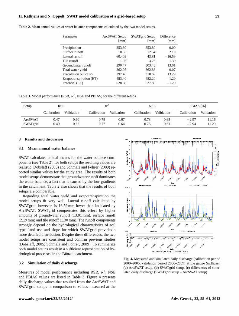
Measures of model performance including RSR,R2, NSEand PBIAS values are listed in Table3. Figure4 presentsdaily discharge values that resulted from the ArcSWAT andSWATgrid setups in comparison to values measured at the

Fig. 4. Measured and simulated daily discharge (calibration period2000–2005, validation period 2006–2009) at the gauge Sarlhusen(a) ArcSWAT setup,(b) SWATgrid setup,(c) differences of simu-lated daily discharge (SWATgrid setup – ArcSWAT setup).



gauge Sarlhusen. Overall comparison of daily discharge sim-ulation values (2000–2009) resulted in a high coefficient ofdetermination (R2

= 0.99).The model evaluation indices RSR,R2 and NSE demon-

strate that simulated and measured daily discharge agree wellfor both the calibration and the validation period. The indicesalso indicate that the ArcSWAT setup performs slightly bet-ter that the SWATgrid setup. This might be explained by twofacts: (1) values of summer and winter peak flows are higherin ArcSWAT; (2) ArcSWAT shows a faster and more realisticrecession of discharge (see also Fig.4). The different propor-tions of fast and slow runoff components (see also Sect.3.1),i.e. surface, lateral and groundwater runoff are generated atHRU or grid-cell level. Thus, modifications that affect thedistribution and composition of land use, soil types and slopedo have an impact on modelled streamflow components.

Values of PBIAS of the different model setups range from−3 to 11 %. The PBIAS differences between the setups areless than 0.2 percentage points; the low number indicatesthat the modelled discharge is insensitive to changing dis-cretization schemes. Drainage density (total channel lengthdivided by drainage area) increases as the number of gridcells or sub-catchments increases. As a result transmissionand deep aquifer losses increase and reduce discharge. Thus,these losses cause the lower runoff calculated by the SWAT-grid setup compared to the ArcSWAT setup (see Table3).Nevertheless, the differences are relatively small comparedto the differences of discharge components caused by thekind of discretization. Similar observations were made byBingner et al.(1997), FitzHugh and Mackay(2000), Chenand Mackay(2004), Jha et al.(2004), Haverkamp et al.(2005), Arabi et al.(2006) andCho et al.(2010).

In summary, model performance statistics shows that sim-ulated and observed daily discharge is similar for both thecalibration and the validation period. The grid-based modelcalculates daily discharge at the catchment outlet accordingto the sub-watershed model. The calibration of the grid-basedmodel using the sub-watershed parameter set resulted ina satisfactory model performance. Statistical indices (RSR,R2, NSE and PBIAS) confirm this finding.

4 Conclusions

The grid-based discretization scheme (SWATgrid) incorpo-rates spatially distributed data into a SWAT model run andenables detailed analysis of every output grid cell at its ge-ographical position. The grid-based setup significantly in-creases the model computation time. While the conventionalArcSWAT model run takes 30 s on a single 2.67 GHz proces-sor, the SWATgrid setup lasts about 12 h per year of simu-lation; therefore calibration using existing guidelines is im-practical.

A time efficient procedure to calibrate grid-based setupswas evaluated in a lowland catchment in Northern Germany.

An ArcSWAT interface was applied to provide an initial, un-calibrated sub-watershed setup. Afterwards, the most sensi-tive parameters to water balance were obtained using SWAT-CUP. The sub-watershed setup then was calibrated with es-tablished manual and automatic calibration techniques. Theresulting parameter set was transferred to a grid-based setupusing the SWATgrid interface.

The Bunzau catchment, a sub-watershed of the River Elbe,served as a test site to evaluate the proposed methodology.Model performance according to (Moriasi et al., 2007) wasderived using statistical indices (RSR,R2, NSE and PBIAS).All indices showed a satisfactory model performance.

Daily discharge derived from the grid configurationmatched well with the sub-watershed discharge (ArcSWATsetup) at the catchment outlet (R2

= 0.99). Thus, establishedsub-watershed calibration techniques (Santhi et al., 2001;Moriasi et al., 2007; Neitsch et al., 2011b) can be used toobtain a parameter set for a grid-based SWAT setup. The re-sults presented, however, are limited to the study area; furtherstudies could compare this calibration method with a “real”grid-based model calibration to confirm these findings.

Acknowledgements.The authors would like to thank the De-partment of Hydrology and Water Resources Management (KielUniversity) and the Schleswig-Holstein state offices LLUR, LKNand LVA for providing the data sets. We also express our gratitudefor the efforts of the reviewers.

Edited by: K. Schneider and S. AchleitnerReviewed by: two anonymous referees

References

Abbaspour, K. C.: User Manual for SWAT-CUP, SWAT Calibrationand Uncertainty Analysis Programs, Swiss Federal Institute ofAquatic Science and Technology, EAWAG, Dubendorf, Switzer-land, 2007.

Arabi, M., Govindaraju, R. S., Hantush, M. M., and Engel, B. A.:Role of watershed subdivision on modeling the effectiveness ofbest management practices with SWAT, J. Am. Water Resour.As., 42, 513–528, 2006.

Arnold, J. G., Srinivasan, R., Muttiah, R. S., and Williams, J. R.:Large area hydrologic modeling and assessment part I: modeldevelopment, J. Am. Water Resour. As., 34, 73–89, 1998.

Arnold, J., Allen, P., Volk, M., Williams, J., and Bosch, D.: Assess-ment of different representations of spatial variability on SWATmodel performance, T. ASABE, 53, 1433–1443, 2010.

Beven, K. J. and Kirkby, M. J.: A physically based, variable con-tributing area model of basin hydrology, Hydrolog. Sci. Bull.,24, 43–69, 1979.

Bingner, R., Garbrecht, J., Arnold, J., and Srinivasan, R.: Effect ofWatershed Subdivision on Simulation Runoff and Fine SedimentYield, Transactions of the American Society of Agricultural En-gineers, 40, 1329–1335, 1997.



Chen, E. and Mackay, D. S.: Effects of distribution-based param-eter aggregation on a spatially distributed agricultural nonpointsource pollution model, J. Hydrol., 295, 211–224, 2004.

Cho, J., Lowrance, R. R., Bosch, D. D., Strickland, T. C., Her,Y., and Vellidis, G.: Effect of Watershed Subdivision and FilterWidth on SWAT Simulation of a Coastal Plain Watershed, J. Am.Water Resour. As., 46, 586–602, 2010.

Cohen, J.: A Coefficient of Agreement for Nominal Scales, Educ.Psychol. Meas., 20, 37–46, 1960.

Dobslaff, N.: GIS-basierte Modellierung von Wasserhaushalt undAbflussbildung am Beispiel des Einzugsgebietes der oberen Stor,Diploma thesis, Department of Hydrology and Water ResourcesManagement, Kiel University, 2005.

DWD: Weather and Climate Data from the German Weather Ser-vice – Station Gnutz (1997–2006), Neumunster (1997–2007) andPadenstedt (2007–2010), Deutscher Wetterdienst, 2011.

Finnern, J.: Boden und Leitbodengesellschaften desStoreinzugsgebietes in Schleswig-Holstein – Vergesellschaftungund Stoffaustragsprognose (K, Ca, Mg) mittels GIS, Disser-tation, Institut fur Pflanzenernahrung und Bodenkunde, KielUniversity, 1997.

FitzHugh, T. W. and Mackay, D. S.: Impacts of input parameterspatial aggregation on an agricultural nonpoint source pollutionmodel, J. Hydrol., 236, 35–53, 2000.

Gassman, P. W., Reyes, M. R., Green, C. H., and Arnold, J. G.:The Soil and Water Assessment Tool: historical development, ap-plications, and future research directions, T. ASABE, 50, 1211–1250, 2007.

Gupta, H. V., Sorooshian, S., and Yapo, P. O.: Status of AutomaticCalibration for Hydrologic Models: Comparison with MultilevelExpert Calibration, J. Hydrol. Eng., 4, 135–143, 1999.

Haverkamp, S., Fohrer, N., and Frede, H.-G.: Assessment of the ef-fect of land use patterns on hydrologic landscape functions: acomprehensive GIS-based tool to minimize model uncertaintyresulting from spatial aggregation, Hydrol. Process., 19, 715–727, 2005.

Jha, M., Gassman, P., Secchi, S., Gu, R., and Arnold, J.: Effect ofwatershed subdivision on SWAT flow, sediment, and nutrient pre-dictions, J. Am. Water Resour. As., 40, 811–825, 2004.

Krysanova, V. and Arnold, J. G.: Advances in ecohydrological mod-elling with SWAT-a review, Hydrolog. Sci. J., 53, 939–947, 2008.

LKN: Daily Discharge Data from the State Office for Coastal Pro-tection, National Park and Marine Protection – Gauging StationSarlhusen (Number 114131), Landesbetrieb fur Kustenschutz,Nationalpark und Meeresschutz Schleswig-Holstein, 2011.

LLUR: Soil Map (1 : 25.000) of Schleswig-Holstein from theAgency for Nature and Environment Schleswig-Holstein, Lan-desamt fur Landwirtschaft, Umwelt und landliche Raume desLandes Schleswig-Holstein, 2010.

LVermA: ATKIS-DEM 5 m grid size Derived from LiDAR Data,Land Survey Office Schleswig-Holstein, Landesamt fur Vermes-sung und Geoinformation Schleswig-Holstein, 2008.

Moriasi, D. N., Arnold, J. G., Liew, M. W. V., Bingner, R. L.,Harmel, R. D., and Veith, T. L.: Model Evaluation Guidelinesfor Systematic Quantification of Accuracy in Watershed Simula-tions, T. ASABE, 50, 885–900, 2007.

Nash, J. and Sutcliffe, J.: River flow forecasting through conceptualmodels part 1 – A discussion of principles, J. Hydrol., 10, 282–290, 1970.

Neitsch, S. L., Arnold, J. G., Kiniry, J. R., Srinivasan, R., andWilliams, J. R.: Soil and Water Assessment Tool Input/OutputFile Documentation: Version 2009, Texas Water Ressources In-stitute Technical Report 365, Texas A&M University System,College Station (Texas), 2011a.

Neitsch, S. L., Arnold, J. G., Kiniry, J. R., and Williams, J. R.: Soiland Water Assessment Tool Theoretical Documentation Version2009, Texas Water Ressources Institute Technical Report 406,Texas A&M University System, College Station (Texas), 2011b.

Oppelt, N., Rathjens, H., and Dornhofer, K.: Integration of landcover data into the open source model SWAT, in: Proceedingsof the First Sentinel-2 Preparatory Symposium held on 23–27 April 2012 in ESA-ESRIN, Frascati, Italy, SP707, DVD Pub-lication, 2012.

Rathjens, H. and Oppelt, N.: SWATgrid: An interface for setting upSWAT in a grid-based discretization scheme, Comput. Geosci.,Comput. Geosci., 45, 161–167, 2012.

Refsgaard, J. and Storm, B.: Computer Models of Watershed Hy-drology, chap. MIKE SHE, 809–846, Water Resources Publica-tions, Colorado, USA, 1995.

Santhi, C., Arnold, J. G., Williams, J. R., Dugas, W. A., Srinivasan,R., and Hauck, L. M.: Validation of the swat model on a largeriver basin with point and nonpoint sources, J. Am. Water Resour.As., 37, 1169–1188, 2001.

Schmalz, B. and Fohrer, N.: Comparing model sensitivities of dif-ferent landscapes using the ecohydrological SWAT model, Adv.Geosci., 21, 91–98, doi:10.5194/adgeo-21-91-2009, 2009.

Schulla, J.: Hydrologische Modellierung von Flussgebieten zur Ab-schatzung der Folgen von Klimaanderungen, Ph.D. thesis, Ge-ographisches Institut, ETH Zurich, 1997.

Singh, J., Knapp, H. V., and Demissie, M.: Hydrologic Modeling ofthe Iroquois River Watershed Using HSPF and SWAT, IllinoisState Water Survey Contract Report 2004-08, Illinois Depart-ment of Natural Resources and Illinois State Geological Survey,2004.

Soil Conservation Service Engineering Division: Section 4: Hydrol-ogy, in: National Engineering Handbook, 1972.

Winchell, M., Srinivasan, R., Di Luzio, M., and Arnold, J. G.: Arc-SWAT Interface For SWAT 2009: User’s Guide, Texas Agricul-tural Experiment Station (Texas) and USDA Agricultural Re-search Service (Texas), Temple (Texas), 2010.


http://dx.doi.org/10.5194/adgeo-21-91-2009

Documents

SWAT model calibration of a grid-based setup