This content has been downloaded from IOPscience. Please scroll down to see the full text.

Download details:

IP Address: 92.136.80.222

This content was downloaded on 22/01/2014 at 08:36

Please note that terms and conditions apply.

Swarming, schooling, milling: phase diagram of a data-driven fish school model

View the table of contents for this issue, or go to the journal homepage for more

2014 New J. Phys. 16 015026

(http://iopscience.iop.org/1367-2630/16/1/015026)

Home Search Collections Journals About Contact us My IOPscience

Swarming, schooling, milling: phase diagramof a data-driven fish school model

Daniel S Calovi1,2,7, Ugo Lopez1,2,3, Sandrine Ngo4, Clément Sire5,6,Hugues Chaté4 and Guy Theraulaz1,2

1 Centre de Recherches sur la Cognition Animale, UMR-CNRS 5169, Université Paul Sabatier,118 Route de Narbonne, F-31062 Toulouse Cedex 4, France2 CNRS, Centre de Recherches sur la Cognition Animale, F-31062 Toulouse, France3 LAPLACE (Laboratoire Plasma et Conversion d’Energie), Université Paul Sabatier,118 route de Narbonne, F-31062 Toulouse Cedex 9, France4 Service de Physique de l’Etat Condensé, CNRS URA 2464, CEA—Saclay,F-91191 Gif-sur-Yvette, France5 Laboratoire de Physique Théorique, UMR-CNRS 5152, Université Paul Sabatier,F-31062 Toulouse Cedex 4, France6 CNRS, Laboratoire de Physique Théorique, F-31062 Toulouse, FranceE-mail: daniel.calovi@gmail.com

Received 7 August 2013, revised 20 November 2013Accepted for publication 26 November 2013Published 21 January 2014

New Journal of Physics 16 (2014) 015026

doi:10.1088/1367-2630/16/1/015026

AbstractWe determine the basic phase diagram of the fish school model derived fromdata by Gautrais et al (2012 PLoS Comput. Biol. 8 e1002678), exploringits parameter space beyond the parameter values determined experimentallyon groups of barred flagtails (Kuhlia mugil) swimming in a shallow tank. Amodified model is studied alongside the original one, in which an additionalfrontal preference is introduced in the stimulus/response function to accountfor the angular weighting of interactions. Our study, mostly limited to groupsof moderate size (in the order of 100 individuals), focused not only on thetransition to schooling induced by increasing the swimming speed, but alsoon the conditions under which a school can exhibit milling dynamics and thecorresponding behavioural transitions. We show the existence of a transitionregion between milling and schooling, in which the school exhibits multistabilityand intermittence between schooling and milling for the same combination of

7 Author to whom any correspondence should be addressed.

Content from this work may be used under the terms of the Creative Commons Attribution 3.0 licence.Any further distribution of this work must maintain attribution to the author(s) and the title of the work, journal

citation and DOI.

New Journal of Physics 16 (2014) 0150261367-2630/14/015026+15$33.00 © 2014 IOP Publishing Ltd and Deutsche Physikalische Gesellschaft

New J. Phys. 16 (2014) 015026 D S Calovi et al

individual parameters. We also show that milling does not occur for arbitrarilylarge groups, mainly due to a distance dependence interaction of the model andinformation propagation delays in the school, which cause conflicting reactionsfor large groups. We finally discuss the biological significance of our findings,especially the dependence of behavioural transitions on social interactions,which were reported by Gautrais et al to be adaptive in the experimentalconditions.

S Online supplementary data available from stacks.iop.org/NJP/16/015026/mmedia

1. Introduction

Transitions between different types of collective behaviour play a major role in the adaptivenessof animal groups [1, 3] (see [2]8). These transitions are commonly observed when animalgroups shift from one collective behaviour to another either spontaneously or in response toa threat. For instance in fish schools, individuals may adopt different spatial patterns whenthey are travelling, feeding or displaying defensive behaviour [4–9]. It is commonly observedthat periods of swarming associated with feeding behaviour, where the group remains cohesivewithout being polarized, are often interspersed with brief periods of schooling during which fishsearch for food and move from one place to another [4]. The actual mechanisms and behaviouralrules that trigger such transitions are still poorly understood.

Several models of collective motion have been introduced in this context. For instance,in the Aoki–Couzin model [10, 11], sharp transitions in collective behaviour are observed forsmall parameter changes. In this zonal model, slight variations in the width of the alignmentzone which controls the alignment behaviour of fish to their neighbours can yield drasticchanges of the structure and polarization of the school, such as transitions between schooling,milling (collective vortex formation) and swarming. In the physics literature, transitions betweendifferent types of collective behaviour are often described as phase transitions. A well studiedcase is the transition to orientational order observed in the popular Vicsek model [12–14].Similar transitions have been described in self-propelled particle models by varying the valueof parameters such as the blind angle [15], individual speed [16] or a ‘strategy parameter’ [17],which ponders a behavioural compromise between aligning with neighbours and reacting totheir direction changes.

All the above models suffer from a lack of experimental validation, having often beendeveloped in a very general context not particularly in relation to experiments/observations.However, a methodology to build models for animal collective motion from the quantitativeanalysis of trajectories in groups of increasing sizes has been recently proposed [18].Using video tracking of groups of barred flagtails (Kuhlia mugil) in a shallow tank, thestimulus/response function governing an individual’s moving decisions in response to theposition and orientation of neighbours was extracted from two-dimensional trajectory data.It was found that a gradual weighting between alignment (dominant at short distances) andattraction (dominant at large distances) best accounted for the data. It was also found that the

8 Includes bibliographical references and index.

2

New J. Phys. 16 (2014) 015026 D S Calovi et al

parameters governing these two interactions depend on the mean speed of the fish, leading to anincrease in group polarization with swimming speed, a direct consequence of the predominanceof alignment at high speed.

Here we investigate the basic phase diagram of the Gautrais et al (2012) model, exploringits parameter space beyond the parameter values determined from the data. This is done inorder to explore the full range of collective behaviour that could be displayed by the model.Our study is limited to groups of moderate size (in the order of 100 individuals) and focuses,beyond the transition to schooling induced by increasing the swimming speed, on the conditionsunder which a school can exhibit milling dynamics. The non-dimensionalized model reveals thatchanges in swimming speed are equivalent to changing the two social interaction parameterswhile maintaining the noise constant. Exploring the parameter plane defined in this way, wefind four regions with distinctive collective behaviour. We show in particular that, in this model,as in most others, milling does not occur for arbitrarily large groups.

2. Model

Let us first recall the findings of Gautrais et al [18, 19]. Barred flagtails (K. mugil) in acircular 4 m diameter tank with a depth of 1.2 m were video-recorded from above for a fewminutes in groups of one to 30 individuals. In this quasi-two-dimensional geometry, very few‘crossing’ events (with one fish passing under another) were observed. At least five replicateswere performed for each group size. In each experiment, fish synchronized their (mean)swimming speed, and their instantaneous speed (tangential velocity), although fluctuating byapproximately 10–20% around its mean, was found uncorrelated to their turning speed (angularvelocity). This led to the representation of single fish behaviour as a two-dimensional smoothrandom walk in which an Ornstein–Uhlenbeck process [20] acts on the fish angular velocity ω.The angular velocity is mathematically described by the stochastic differential equation

dω(t) = −v

[dt

ξ(ω(t) − ω∗(t)) + σ dW

], (1)

where v is the (constant) swimming speed, dW refers to a standard Wiener process, ξ = 0.024 mis a characteristic persistence length and σ = 28.9 m−1 s−1/2 controls the noise intensity, whereboth ξ and σ have been estimated from experimental data on barred flagtail trajectories. Thelarge-scale properties of this model have been extensively studied by Degond and Motsch[21, 22]

In the above equation, ω∗(t) is the stimulus/response function based on the individualsresponse to the proximity of the tank wall—irrelevant in the following as we shall considergroups evolving in an infinite domain—and on the reaction to the neighbouring fish orientationand distance. It was found that for groups of two fish, these social interactions are well describedby a linear superposition of alignment and attraction with weights depending on di j , the distancebetween the two fish. It was found further that in groups of more than two fish, many-bodyinteractions could be safely approximated by the normalized sum of pair interactions withthose individuals forming the first shell of Voronoi neighbours of the focal fish (figure 1).Mathematically, one has

ω∗=

1

Ni

∑j∈Vi

[kV v sin φi j + kP di j sin θi j

], (2)

3

New J. Phys. 16 (2014) 015026 D S Calovi et al

positional interaction intensity (s-1)

Figure 1. Fish interactions graphical representation used in the model. (a) The distancedi j of fish j from fish i ; φi j is the relative orientation heading of fish j compared tofish i ; θi j is the angle between the angular position of fish j with respect to fish i . (b)Illustration of the Voronoi neighbourhood, where arrows indicate the fish headings ofthe focal fish (red region) to his first Voronoi neighbours (yellow regions). (c) Positionalinteraction intensity as proposed by Gautrais et al. (d) Positional interaction intensity asgiven by the angular preference.

where Vi is the Voronoi neighbourhood of fish i containing Ni + 1 individuals, φi j = φ j − φi

is the angle between the orientational headings of fish i and j , and θi j is the angle betweenthe heading of fish i and the vector linking fish i to fish j (figure 1). The functional formsinvolving the sine function, chosen for simplicity, were also validated by the data. They ensurethat interactions vanish when the fish are already aligned or in front of each other as can be seenin figure 1(c).

Note there is a speed dependence on the alignment, and hence a tendency to producepolarized groups at large speeds. A similar positive correlation between group speed and polarityhas also been found in groups of giant danios (Devario aequipinnatus) and golden shiners(Notemigonus crysoleucas) [23, 24].

Note also that the strength of the attractive positional interaction, scaled by kP , increaseslinearly with di j , which is rather unrealistic: if two fish were very far apart, they would turnat extremely large speeds towards each other. Moreover, attraction is of the same amplitudewhether fish j is in front or behind fish i , which may also look unrealistic, as one might expectfish i to be less ‘aware’ and attracted to fish j if j is behind i . Nevertheless this form of attractioninteraction was found to account well for the data, because in the experimental tank fish nevergo far away from each other.

4

New J. Phys. 16 (2014) 015026 D S Calovi et al

However, a careful analysis of the data in pairs of two fish revealed that the behaviouralreactions of a focal fish depend on the angular position of its neighbour (θi j ) even if the resultingimpact on collective motion in larger groups cannot be detected in a confined environment. Sowe will consider the possibility of an angular weighting of the interactions in the form of anextra multiplicative factor

�i j = 1 + cos(θi j) (3)

to the interaction term ω∗(t), so that (1) is rewritten as

dω(t) = −v

[dt

ξ

(ω(t) − �i jω

∗(t))

+ σ dW

]. (4)

The function �i j was designed to ensure a frontal preference and some kind of rear blind angle.Its specific form (which can be seen in figure 1(d)) was chosen for its simplicity and its unitangular average.

In the following, we perform numerical simulations of the model, varying its keyparameters: the swimming speed v, and kP and kV , the behavioural parameters controllingattraction and alignment. Most of our study is restricted to moderate-size groups of N = 100fish. However, we also present results as a function of group size when investigating therobustness of milling (section 6). Typically, a set of 100 random initial conditions is simulatedover a period of 1000 s, where the first half of each series was discarded to account for transientbehaviour.

The polarization of the school is quantified by the global polar order parameter

P =1

N

∣∣∣∣∣N∑

i=1

Evi

v

∣∣∣∣∣ , (5)

which reaches order 1 values for strongly polarized, schooling groups. Milling behaviour isdetected via the global normalized angular momentum

M =1

N

∣∣∣∣∣N∑

i=1

Eri × Evi

|Eri |v

∣∣∣∣∣ , (6)

which will tend towards unity when the school is rotating in a single vortex. As we shall see,the two scalar, positive, quantities P and M often play symmetric roles in the ordered phases ofthe groups: a schooling group will show large P and negligible M , and the opposite is true fora milling group.

3. Speed-induced transition to schooling

We first report the basic transition from swarming to schooling observed when increasing theswimming speed of individuals. Already observed in [18], it is a natural consequence of thepredominance of the alignment interaction at high speeds. Here, we confirm the existence of thetransition in the absence of walls confining the group. Figure 2 summarizes our results for N =

100 individuals, using the parameter values determined from the experimental data obtained insmaller groups (kV = 2.7 m−1, kP = 0.41 m−1 s−1, ξ = 0.024 m and σ = 28.9 m−1 s−1/2), with andwithout the angular preference function �.

5

New J. Phys. 16 (2014) 015026 D S Calovi et al

(a)

(b)

(c)

0.0

0.4

0.8

Pol

ariz

atio

n

0.00

0.10

0.20

0.30

Mill

ing

0.0 0.2 0.4 0.6 0.8 1.0 1.2

0.0

0.5

1.0

1.5

Speed (m/s)

Ave

rage

nei

ghbo

ur d

ista

nce

(m)

Without frontal preferenceWith angular preference

Figure 2. (a) Displays the polarization parameter as a function of the speed v, forsimulations with the original model (blue) and the angular preference (red), where acollective state transition to schooling can be seen in both cases, although more abruptlyin the original model (blue line). (b) Milling parameter for both simulations (blue,original model and red, with the angular preference) as a function of the speed. Oneobserves that in the transition zone (v ≈ 0.2 m s−1) there is an increase in milling valuesin the simulations with angular preference (red). (c) Average distance to the neighboursfor both sets of simulations. We performed ten replicates for each different speed, andall simulations had 107 iterations, where we discarded the first half of the data, and usedonly one datapoint for every ten iterations.

We find that the transition to schooling occurs at a speed range of zero to four body lengthsper second, a reasonable one considering the barred flagtail swimming ability (figure 2(a)). Thetransition is smoother with angular preference (red curves) and consequently requires larger

6

New J. Phys. 16 (2014) 015026 D S Calovi et al

speed values to reach similar results as the original model. Even though no pronounced millingis found in either cases of figure 2(b), a more pronounced result is achieved with the angularpreference, which seems to directly influence the school distance to the centroid in figure 2(c).

4. Non-dimensionalization of the model

In order to get more insight into how speed affects the relative importance of noise, directionaland positional behavioural reactions, we rewrite the model in a non-dimensionalized form. Aftera straightforward manipulation we are left with only three independent parameters:

α = ξ 3σ 2/v, β = (kV v)/(ξ 2σ 2) and γ = (kPv)/(ξ 4σ 4) . (7)

The time step dt̃ = dt/(ξ 2σ 2) has no influence on the simulations provided it is small enough.For all simulations we used dt̃ = 0.1α for α < 0.1 or dt̃ = 0.01 for the remaining cases. Thefull set of non-dimensionalized equations reads

α dω̃(t̃) = dt̃(ω̃(t̃) − ω̃∗(t̃)

)+ dW, (8)

where dW refers to a standard Wiener process. The term ω̃∗ can be rewritten as

ω̃∗=

1

Ni

∑j∈Vi

[β sin φi j + γ d̃i j sin θi j

]. (9)

Note that in our equivalent system, time is now counted in units of a typical time t̃ = v(ξσ )−2,defined with the correlation length ξ and noise amplitude σ . The distance is expressed in unitsof a typical length x̃ = v(ξσ )−2, which is simply the displacement of a fish during time t̃with speed/velocity v. The angular speed and thus the evolution of the fish orientation aredetermined by the relative weight of equivalent alignment (β) and positional (γ ) intensity overthe equivalent angular inertia term α.

The expressions of the non-dimensionalized coefficients show that increasing speed,while keeping other parameters constant, leads to an increase in the equivalent positionaland alignment interactions. At the same time it reduces the angular inertia while keeping theequivalent noise amplitude/intensity constant. The speed induced transition can thus be seen asa competition between noise and social interactions.

Hereafter we perform an extensive study of the non-dimensionalized version of the model,with particular attention paid to the emergence of significant milling.

5. Phase diagram in the space of behavioural parameters

We explored the parameter plane formed by coefficients β and γ in the domain [0, 5] × [0, 5]including the experimentally determined values kV = 2.7 m−1 (β ≈ 2.24) and kP = 0.41 m−1s−1

(γ ≈ 0.71) by steps of 0.2, yielding the 26 × 26 grid of results shown in figure 3. Theangular inertia term was set at α ≈ 0.014, equivalent to the experimentally reasonable valuev = 0.8 m s−1.

Two cases are presented, without and with the angular weighting function � (left andright panels respectively). In both cases, a transition to schooling is observed as β is increased

7

New J. Phys. 16 (2014) 015026 D S Calovi et al

Figure 3. Statistics for simulations made for different alignment and positionalparameters (β and γ respectively), both in the interval [0, 5] with an increment of 0.2 (inboth β and γ units respectively). Simulations were made with an angular inertia termof α ≈ 0.014 (equivalent to a speed v = 0.8 m s−1). The colour code bars on the rightrepresent the values for the respective statistics on the left (polarization, milling andaverage distance to the neighbours). The left column represents different statistics forthe original model as seen in (1), while the right column graphs represent simulationswith angular preference as seen in (4). The statistics here represented are: (a) and (b)polarization parameter; (c) and (d) milling parameter; (e) and (f) average neighbourdistance. Each datum point is the result of an average over 100 different simulations,where the first half of each simulation was discarded to avoid transitional behaviour,resulting in a total of 2×106 data points for every parameter configuration.

(figures 3(a) and (b)). Such a transition is virtually independent of γ considering the originalmodel (figure 3(a)) while presenting a functional form for simulations using the angularpreference (figure 3).

8

New J. Phys. 16 (2014) 015026 D S Calovi et al

A strong qualitative difference is nevertheless observed between the left and the rightpanels in figures 3(c) and (d). With the angular dependence � (right panels), outright schoolingis preceded by a large region where milling is observed (3(d)), whereas no significant millingoccurs without angular weighting (3(c)). This may not seem too surprising given that � favoursthe formation of (local) columns in which fish follow those in front of them.

Lastly, we observe a peculiar property in figures 3(e) and (f), which show the averagedistance to neighbours. With the angular preference (figure 3(f)), the region of low β exhibits aweak ridge bordering the swarming region (γ and β ≈ 0) where the average distance is expectedto diverge. This ridge extends to high γ values for which one would infer small-size schoolsand shorter neighbour distances. One should be aware that the colour codes presented on theselast two figures are presented on a logarithmic scale. This was introduced since a divergenceoccurs in the swarming region, which would mask secondary ridges, such as the one found infigure 3(f).

The explanation, despite being initially counterintuitive, is rather simple. Despite theγ -induced tendency to stay together, a low β means that fish have a lower tendency to disturbtheir alignment to match that of their neighbours, meaning that fish will rely mostly on thepositional interaction. This implies that if a neighbour is directly ahead or behind the focalfish, there is no need to change the direction of motion. Also, both cases (with or withoutangular preference) have zero interaction for anti-parallel neighbours. This means that whenγ dominates the interactions, the stable fish configuration is a line. Having noise in (1) or (4)leads to fish organizing themselves in a quasi-unidimensional configuration, and the fish infront, not having additional neighbours on their sides, will eventually turn due to noise. After aslight turn, this fish will now have new Voronoi neighbours, with fish previously located behindit now located slightly to its side, and make a 180◦ turn to recover the optimal configuration.This mechanism leads fish to organize themselves in two columns going in opposite directionsconnected at the end of the school by this ‘U turn’ (see snapshot in figure 4(c), panel III).

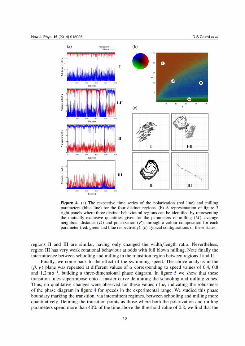
To visualize the above results in a synthetic way, we took advantage of the fact that themain behavioural regions apparent in figures 3(b), (d) and (f) are distinguished by mutuallyexclusive quantities: when schooling is strong, milling is weak and the distance to neighbours(D) is small; when milling is strong, schooling is weak and D is small; when D is larger,both schooling and milling are weak. This mutual exclusion of schooling and milling is clearin the time series shown in figure 4(a). We thus constructed the following composite orderparameter:

S(P, M, D) = P + M exp[i 2π/3] + D exp[i 4π/3] (10)

which takes complex values such that the phase codes for the behaviour and the modulus forthe intensity of this behaviour, where the average distance was normalized according to thelargest value observed. As a result, the information of the right panels of figure 3 is representedsynthetically in figure 4(b). Three distinct regions are clearly apparent as each is representedin a different colour (red for polarization, blue for milling and green for average neighbourdistance). Typical configurations of the group corresponding to the time-series of figure 4(a)are shown in figure 4(c). (See also the movies in the supplementary material (available fromstacks.iop.org/NJP/16/015026/mmedia), appendices A.1–A.4, for simulations of these fourtypes of behaviour.)

Regions I and II refer to the schooling and milling states respectively. Region IIIrefers to the winding (line configuration) state mentioned previously. It could be argued that

9

New J. Phys. 16 (2014) 015026 D S Calovi et al

Figure 4. (a) The respective time series of the polarization (red line) and millingparameters (blue line) for the four distinct regions. (b) A representation of figure 3right panels where three distinct behavioural regions can be identified by representingthe mutually exclusive quantities given for the parameters of milling (M), averageneighbour distance (D) and polarization (P), through a colour composition for eachparameter (red, green and blue respectively). (c) Typical configurations of these states.

regions II and III are similar, having only changed the width/length ratio. Nevertheless,region III has very weak rotational behaviour at odds with full blown milling. Note finally theintermittence between schooling and milling in the transition region between regions I and II.

Finally, we come back to the effect of the swimming speed. The above analysis in the(β, γ ) plane was repeated at different values of α corresponding to speed values of 0.4, 0.8and 1.2 m s−1, building a three-dimensional phase diagram. In figure 5 we show that thesetransition lines superimpose onto a master curve delimiting the schooling and milling zones.Thus, no qualitative changes were observed for these values of α, indicating the robustnessof the phase diagram in figure 4 for speeds in the experimental range. We studied this phaseboundary marking the transition, via intermittent regimes, between schooling and milling morequantitatively. Defining the transition points as those where both the polarization and millingparameters spend more than 40% of the time above the threshold value of 0.8, we find that the

10

New J. Phys. 16 (2014) 015026 D S Calovi et al

0

5

10

15

20

25

30

0 10 20 30 40 50 60 70 80

β

γ

Transition, v = 0.4 m/sTransition, v = 0.8 m/sTransition, v = 1.2 m/s

Fitted transition

Schooling state

Milling state

Figure 5. Transition between region schooling and milling states for differentspeeds. A functional form (A

√γ + B) fitted for v = 0.8 m s−1 proved to also properly

describe the transitions for speeds of 0.4 and 1.2 m s−1, where A = 3.22 ± 0.05 andB = −2.23 ± 0.26.

transition line, for all values of v studied, can be fitted by the simple functional form

β = A√

γ + B, (11)

where A and B take values independent of α in the ranges studied (figure 5).Although we do not have a quantitative explanation for the above functional form, these

fits indicate the possibility of a rather simple theory accounting for the full phase diagramof our model. Meanwhile, a qualitative explanation for the dependence on γ is given by theneed to counteract the global polarization tendency given by β, while maintaining a local one.Also, figure 3(a) indicates minimum β × γ values to overcome the noise. In the supplementarymaterial (available from stacks.iop.org/NJP/16/015026/mmedia) there are two videos (movies5 and 6) of the two dimensional histogram evolution for the schooling and millingparameters as we change β or γ while maintaining the other one constant (γ = 17.28 andβ = 13.30), meaning we have respectively vertical and horizontal transition cross-sectionsin figure 5.

6. Group-size-induced transition

In this section, we investigate the influence of group size on the robustness of both millingand schooling behaviour in our model using the angular weighting function. Apart from thegeneral theoretical context mentioned above, this is also of direct relevance for fish, as it hasbeen reported recently that in golden shiners increasing group size significantly increases theamount of time spent in a milling state [24].

11

New J. Phys. 16 (2014) 015026 D S Calovi et al

161284

161284

(a)

(b)

0.0

0.2

0.4

0.6

0.8

1.0

Pol

ariz

atio

n

10 20 50 100 200 500 2000 5000

0.0

0.2

0.4

0.6

0.8

1.0

Number of fish

Mill

ing

Figure 6. Simulations done for a fixed γ ≈ 4.5 with an angular inertia term of α ≈ 0.014(equivalent to a speed v = 0.8 m s−1) for different quantities of fish and β values, where(a) and (b) refer to the milling and polarization parameters respectively.

We performed a series of simulations at fixed γ ≈ 4.5 with an angular inertia termα ≈ 0.014 (equivalent to a speed v = 0.8 m s−1). Figure 6 shows the milling and schoolingorder parameters for simulations of groups from 10 to 4000 fish. These results indicate thatthere exists an inferior limit of approximately 60 fish in order to achieve significant milling andthat this behaviour progressively disappears at large sizes. Although these results must be taken

12

New J. Phys. 16 (2014) 015026 D S Calovi et al

with care given the unbounded character of the variation of positional interaction with distanceto neighbours, they show that for up to 100 fish, increasing group size induces a transition fromschooling to milling for β 6 8. For larger values of the alignment parameter, despite havinghigher overall values for the milling parameter, the transition does not occur. This indicates thatin the model studied here, like in many of those proposed before [25], milling dynamics doesnot emerge in the arbitrarily large infinite-size limit.

Although such a statement has obvious interest for physicists, we believe it bears someimportance regarding animal group behaviour. Also, it is worth noting that the variation in themilling parameter seen for β > 12 in figure 6(a) happens as the duration of the milling andschooling behaviour increases with N . Such an increase is so intense that for simulations withmore than 300 fish, usually only one type of behaviour can be seen for every initial condition,giving a very large standard deviation and a highly fluctuating average. Furthermore, somesimulations for N > 1000 displayed more than one vortex at the same time, patterns which themilling parameter cannot account for. One can see in figure 6(b) that the schooling behaviouris affected by the size as well. This again is due to the effect of large schools. This stretch onschool extensions enables information propagation delays, which in turn, cause reductions onthe global polarization parameter. It is easy to see how a three dimensional configuration couldachieve lower extensions with large fish quantities, which would in turn minimize these effects.

7. Conclusions

Understanding how complex motion patterns in fish schools arise from local interactions amongindividuals is a key question in the study of collective behaviour [26, 27]. In a previous work,Gautrais et al have determined the stimulus/response function that governs an individual’smoving decisions in barred flagtails (K. mugil) [18]. It has been shown that two kinds ofinteractions controlling the attraction and the alignment of fish are involved and that they areweighted continuously depending on the position and orientation of the neighbouring fish. It hasalso been found that the magnitude of these interactions changes as a function of the swimmingspeed of fish and the group size. The consequence being that groups of fish adopt differentshapes and motions: group polarization increases with swimming speed while it decreases asgroup size increases.

Here we have shown that the relative weights of the attraction and alignment interactionsplay a key role in the emergent collective states at the school level. Depending on the magnitudeof the attraction and the alignment of fish to their neighbours, different collective states can bereached by the school. The exploration of the parameter space of the Gautrais et al model revealsthe existence of two dynamically stable collective states: a swarming state in which individualsaggregate without cohesion, with a low level of polarization, and a schooling state in whichindividuals are aligned with each other and with a high level of polarization. The transitionbetween the two states is induced by an increase of the swimming speed. Furthermore, theaddition in the model of a frontal preference to account for the angular weighting of interactionsleads to two other collective states: a milling state in which individuals constantly rotate aroundan empty core thus creating a torus and a winding state, in which the group self-organizes intoa linear crawling structure. This last group structure is reminiscent of some moving patternsobserved in the Atlantic herring (Clupea harengus) [28].

Of particular importance is the transition region between milling and schooling. In thisregion, the school exhibits multistability and it regularly shifts from schooling to milling for

13

New J. Phys. 16 (2014) 015026 D S Calovi et al

the same combination of individual parameters. This particular property was recently reportedin experiments performed in groups of golden shiners [24]. Our results show that the transitionregion can be described by a simple functional form describing the respective weights of thealignment and attraction parameters and is independent of the fish swimming speed in theexperimental range. The modulation of the strength of the alignment and attraction may dependon the behavioural and physiological state of fish [29]. In particular, various environmentalfactors such as a perceived threat may change the way fish respond to their neighbours andhence lead to dramatic changes in collective motion patterns at the school level [30, 31].

Finally, we show that collective motion may dramatically change as group size increases.The absence of a milling state in the largest groups is a natural consequence of the spatialconstraints exerted upon individuals’ movements as the number of fish exceeds some criticalvalue. These constraints could be much less stringent in three dimensions, as testified bythe observation of cylindrical vertical milling structures involving several thousands of fishin bigeye trevally (Caranx sexfasciatus). With an additional dimension, the same numberof fish could result in a mill of much smaller diameter, not only avoiding the problems ofdistance dependence, but also minimizing information propagation delays and the emergenceof competing behaviour.

A more in depth physics study of the transitions presented here is necessary. Unfortunately,the present model is restricted to schools of biologically relevant sizes (N ≈ 100 fish) preventingsuch analysis for the current social interactions. In this manner, additional changes to the modelare required, among them are: (i) eliminating the linear distance dependence on the interactions,by either implementing a saturation or a decay to this interaction; (ii) changing the boundaryconditions for periodic ones to avoid evaporating schools once the distance dependence isremoved; and (iii) a three dimensional study of the model to check the impact of an additionallevel of freedom on the school behaviour.

Acknowledgments

We are grateful to Jacques Gautrais, Alfonso Pérez-Escudero and Sepideh Bazazi for commentson the manuscript. DSC was funded by the Conselho Nacional de Desenvolvimento Científicoe Tecnológico—Brazil. UL was supported by a doctoral fellowship from the scientific councilof the Université Paul Sabatier. This study was supported by grants from the Centre National dela Recherche Scientifique and Université Paul Sabatier (project Dynabanc).

References

[1] Couzin I D and Krause J 2003 Self-organization and collective behavior in vertebrates Adv. Stud. Behav.32 1–75

[2] Sumpter D J T 2010 Collective Animal Behavior (Princeton, NJ: Princeton University Press) p 302[3] Solé R V 2011 Phase Transitions (Princeton, NJ: Princeton University Press) p 264[4] Radakov D V 1973 Schooling and Ecology of Fish (New York: Wiley) p 173[5] Pitcher T J 1993 Behavior of Teleost Fishes (London: Chapman and Hall)[6] Parrish J K and Edelstein-Keshet L 1999 Complexity, pattern and evolutionary trade-offs in animal

aggregation Science 284 99–101[7] Freon P and Misund O A 1999 Dynamics of Pelagic Fish Distribution and Behaviour: Effects on Fisheries

and Stock Assessment (Fishing News Books) (Oxford: Wiley-Blackwell)

14

New J. Phys. 16 (2014) 015026 D S Calovi et al

[8] Parrish J K, Viscido S V and Grunbaum D 2002 Self-organized fish schools: an examination of emergentproperties Workshop on the Limitations of Self-Organization in Biological Systems (11–13 May 2001)(Woods Hole, MA: Marine Biol. Lab.) ; Biol. Bull 202 pp 296–305

[9] Becco Ch., Vandewalle N, Delcourt J and Poncin P 2006 Experimental evidences of a structural anddynamical transition in fish school Physica A 367 487–93

[10] Aoki I 1982 A simulation study on the schooling mechanism in fish Bull. Japan. Soc. Sci. Fish 48 1081–8[11] Couzin I D, Krause J, James R, Ruxton G D and Franks N R 2002 Collective memory and spatial sorting in

animal groups J. Theor. Biol. 218 1–11[12] Vicsek T, Czirók A, Ben-Jacob E, Cohen I and Shochet O 1995 Novel type of phase transition in a system of

self-driven particles Phys. Rev. Lett. 75 1226–9[13] Czirók A, Stanley H E and Vicsek T 1997 Spontaneously ordered motion of self-propelled particles J. Phys.

A: Math. Gen. 30 1375[14] Chaté H, Ginelli F, Grégoire G and Raynaud F 2008 Collective motion of self-propelled particles interacting

without cohesion Phys. Rev. E 77 046113[15] Newman J P and Sayama H 2008 Effect of sensory blind zones on milling behavior in a dynamic self-

propelled particle model Phys. Rev. E 78 011913[16] Mishra S, Tunstrøm K, Couzin I D and Huepe C 2012 Collective dynamics of self-propelled particles with

variable speed Phys. Rev. E 86 011901[17] Szabó P, Nagy M and Vicsek T 2009 Turning with the others: novel transitions in an SPP model with coupling

of accelerations Phys. Rev. E 79 021908[18] Gautrais J, Ginelli F, Fournier R, Blanco S, Soria M, Chaté H and Theraulaz G 2012 Deciphering interactions

in moving animal groups PLoS Comput. Biol. 8 e1002678[19] Gautrais J, Jost C, Soria M, Campo A, Motsch S, Fournier R, Blanco S and Theraulaz G 2009 Analyzing fish

movement as a persistent turning walker J. Math. Biol. 58 429–45[20] Uhlenbeck G E and Ornstein L S 1930 On the theory of the Brownian motion Phys. Rev. 36 823–41[21] Degond P and Motsch S 2008 Large scale dynamics of the persistent turning walker model of fish behavior

J. Stat. Phys. 131 989–1021[22] Degond P and Motsch S 2011 A macroscopic model for a system of swarming agents using curvature control

J. Stat. Phys. 143 685–714[23] Viscido S V, Parrish J K and Grunbaum D 2004 Individual behavior and emergent properties of fish schools:

a comparison of observation and theory Mar. Ecol-Prog. Ser. 273 239–49[24] Tunstrøm K, Katz Y, Ioannou C C, Huepe C, Lutz M J and Couzin I D 2013 Collective states, multistability

and transitional behavior in schooling fish PLoS Comput. Biol. 9 e1002915[25] Lukeman R, Li Y-X and Edelstein-Keshet L 2009 A conceptual model for milling formations in biological

aggregates Bull. Math. Biol. 71 352–82[26] Lopez U, Gautrais J, Couzin I D and Theraulaz G 2012 From behavioural analyses to models of collective

motion in fish schools Interface Focus 2 693–707[27] Delcourt J and Poncin P 2012 Shoals and schools: back to the heuristic definitions and quantitative references

Rev. Fish Biol. Fisher. 22 595–619[28] Gerlotto F et al 2003 Towards a synthetic view of the mechanisms and factors producing the collective

behavior of tropical pelagic fish: individual, school, environment and fishery. Proc. ICES Symp. on FishBehaviour in Exploited Ecosystems (Bergen, Norway) Abstracts p 86

[29] Wendelaar Bonga S E 1997 The stress response in fish Physiol. Rev. 77 591–625[30] Beecham J A and Farnsworth K D 1999 Animal group forces resulting from predator avoidance and

competition minimization J. Theor. Biol. 198 533–548[31] Viscido S V and Wethey D S 2002 Quantitative analysis of fiddler crab flock movement: evidence for ‘selfish

herd’ behaviour Anim. Behav. 63 735–41

15